1

Sensitivity Analysis for Cash Flow Simulation

Based Real Option Valuation

Tero Haahtela

Aalto University, School of Science and Technology

P.O. Box 15500, FI-00076 Aalto, Finland

+358 50 577 1690 tero.haahtela@aalto.fi

Abstract

Sensitivity analysis identifies the critical aspects of the investment model that affect model

output uncertainty. Common sensitivity analysis on options considers how the solution

changes as a result of change in one of the key parameters (underlying asset value, volatility,

exercise price, interest rate, time to maturity, dividends). In case of cash flow simulation

based real options, these are mostly indirect variables that are computed based on the primary

input variables - demand, unit selling price, and unit costs - in the cash flow calculation. The

method presented in this paper combines the uncertainties in the underlying asset together by

simulation, and then uses regression analysis approach for estimating how a change in a

primary variable or variables affects simultaneously the stochastic process parameters of

expected value and volatility during different time periods. As a result, the presented method

shows how a change in a primary variable affects project value with real options. This

information is also essential as it shows decision makers which uncertainties to follow, and

thus this mitigates the common black box syndrome of consolidated cash flow simulation

based methods.

Keywords: real options, sensitivity analysis, cash flow simulation, volatility

JEL Classification: G31, G13

2

1. Introduction

Sensitivity analysis is essential in order to identify the critical aspects of the investment

model that affect model output uncertainty. The purpose in sensitivity analysis is to determine

which input parameters are important and contribute most to the output variability (Helton,

2000). Based on this relative importance, sensitivity analysis provides guidance for further

data collection and modeling (Manache & Melching 2008). Sensitivity analysis reveals under

which conditions the model or with which parameter values the solution is robust, i.e. under

what circumstances the model is insensitive to the changes in input parameters. It helps in

defining under what circumstances the change in operational activities is required, which in

case of real options is required in order to be able to decide on option exercise timely.

Sensitivity analysis may also reveal what is the accuracy of the final model and the degree of

uncertainty (Saltelli et al., 2004). This may be related to data accuracy and model uncertainty,

and this uncertainty is reflected both as ambiguity and volatility uncertainty.

Traditional sensitivity analysis on options considers how the solution changes as a result of

change in one of the parameters of underlying asset value (delta), volatility (vega), exercise

price, time to maturity (theta), and interest (rho). With financial options, these aspects can be

computed using well-known equations and available market information, allowing precise

state-space structure for different underlying asset values for each time period. However, in

case of real options analysis, the parameters affecting the Greeks directly are not the direct

parameters that are changing but rather indirect or secondary parameters, for example

volatility, that are derived from the actual changing primary cash flow calculation input

parameters. The parameters that truly change are those related to cash flow model, e.g.

product demand, sales unit price, and variable unit costs.

Typical for these primary parameters is that when their values change in a cash flow

simulation, they affect simultaneously several of the previously mentioned indirect real

option parameters. Most likely a change in a significant parameter in a cash flow calculation

affects at the same time both the expected underlying asset value and some other parameters

used to describe its stochastic process. Because of the interactions with serial and cross-

correlations in the simulated cash flow calculation, also the stochastic process used to

describe the underlying asset movements may need to be changed. Commonly assumed

geometric Brownian motion may not be appropriate and robust enough, because it does not

handle negative underlying asset values and multiplicativity is not necessarily the most

reliable description of the stochastic process. Also the amount of uncertainty in terms of

underlying asset value ambiguity in the beginning may change.

Sensitivity analysis with simulated cash flow options should be conducted in a way that

shows how the change in a primary parameter, e.g. sales unit price, affects the total value of

3

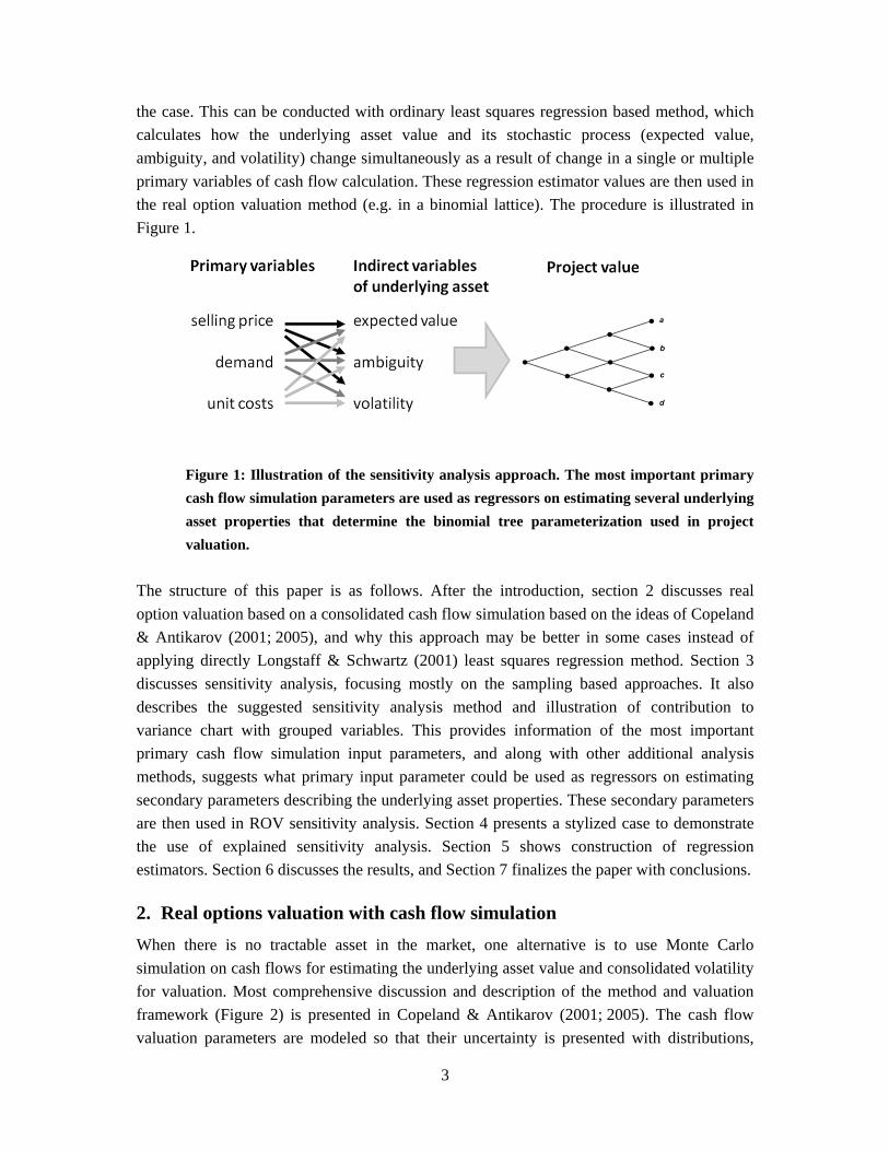
the case. This can be conducted with ordinary least squares regression based method, which

calculates how the underlying asset value and its stochastic process (expected value,

ambiguity, and volatility) change simultaneously as a result of change in a single or multiple

primary variables of cash flow calculation. These regression estimator values are then used in

the real option valuation method (e.g. in a binomial lattice). The procedure is illustrated in

Figure 1.

Figure 1: Illustration of the sensitivity analysis approach. The most important primary

cash flow simulation parameters are used as regressors on estimating several underlying

asset properties that determine the binomial tree parameterization used in project

valuation.

The structure of this paper is as follows. After the introduction, section 2 discusses real

option valuation based on a consolidated cash flow simulation based on the ideas of Copeland

& Antikarov (2001; 2005), and why this approach may be better in some cases instead of

applying directly Longstaff & Schwartz (2001) least squares regression method. Section 3

discusses sensitivity analysis, focusing mostly on the sampling based approaches. It also

describes the suggested sensitivity analysis method and illustration of contribution to

variance chart with grouped variables. This provides information of the most important

primary cash flow simulation input parameters, and along with other additional analysis

methods, suggests what primary input parameter could be used as regressors on estimating

secondary parameters describing the underlying asset properties. These secondary parameters

are then used in ROV sensitivity analysis. Section 4 presents a stylized case to demonstrate

the use of explained sensitivity analysis. Section 5 shows construction of regression

estimators. Section 6 discusses the results, and Section 7 finalizes the paper with conclusions.

2. Real options valuation with cash flow simulation

When there is no tractable asset in the market, one alternative is to use Monte Carlo

simulation on cash flows for estimating the underlying asset value and consolidated volatility

for valuation. Most comprehensive discussion and description of the method and valuation

framework (Figure 2) is presented in Copeland & Antikarov (2001; 2005). The cash flow

valuation parameters are modeled so that their uncertainty is presented with distributions,

4

time series, cross- and auto-correlations. The cash flow is simulated and based on that, both

the expected value and its stochastic process are estimated. Therefore, this procedure

consolidates all the continuously evolving risks into a single deviation measure, consolidated

univariate volatility estimate. The approach is based on the idea that an investment with real

options should be valued as if it was a traded asset in markets even though it would not be

publicly listed. According to Copeland and Antikarov, the present value of the cash flows of

the project without flexibility is the best unbiased estimate of the market value of the project

were it a traded asset. They call this assumption marketed asset disclaimer.

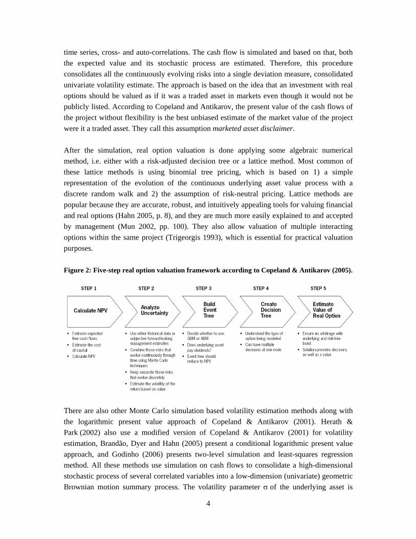
After the simulation, real option valuation is done applying some algebraic numerical

method, i.e. either with a risk-adjusted decision tree or a lattice method. Most common of

these lattice methods is using binomial tree pricing, which is based on 1) a simple

representation of the evolution of the continuous underlying asset value process with a

discrete random walk and 2) the assumption of risk-neutral pricing. Lattice methods are

popular because they are accurate, robust, and intuitively appealing tools for valuing financial

and real options (Hahn 2005, p. 8), and they are much more easily explained to and accepted

by management (Mun 2002, pp. 100). They also allow valuation of multiple interacting

options within the same project (Trigeorgis 1993), which is essential for practical valuation

purposes.

Figure 2: Five-step real option valuation framework according to Copeland & Antikarov (2005).

There are also other Monte Carlo simulation based volatility estimation methods along with

the logarithmic present value approach of Copeland & Antikarov (2001). Herath &

Park (2002) also use a modified version of Copeland & Antikarov (2001) for volatility

estimation, Brandão, Dyer and Hahn (2005) present a conditional logarithmic present value

approach, and Godinho (2006) presents two-level simulation and least-squares regression

method. All these methods use simulation on cash flows to consolidate a high-dimensional

stochastic process of several correlated variables into a low-dimension (univariate) geometric

Brownian motion summary process. The volatility parameter of the underlying asset is

5

estimated by calculating the standard deviation of the simulated probability distribution for

the rate of return.

A good question is whether the consolidated cash flow methods are any better than applying

directly the Longstaff & Schwartz approach for similar cases with several input parameters

and interacting options. Longstaff & Schwartz (2001) approach for valuing American options

uses ordinary least squares regression for estimating forward-looking estimator. Then, at each

time period and for each underlying asset price level, given the combination of regression

estimator input parameter values, a decision is made of the optimal continuing strategy. This

approach is sufficiently flexible and straightforward if the number of options in a case is

small, and the method is also computationally fast. The method can also be applied as a

sensitivity analysis method by changing the regression estimator input parameter values,

which in turn change the expected value according to the estimator.

The shortcoming of the approach is that it is difficult to apply the same method when there

are several interacting sequential and parallel options. Determining a good forward-looking

estimator for the whole project value, especially in the early stages, is difficult if not

impossible, because the estimator should be able to capture the future value including the

forthcoming interacting options. This problem can be mitigated by applying Bellman’s

principle of optimality with backward induction logic. Starting from the end of the project,

regression equations are determined for each stage, and the optimal decision forward-looking

decisions are actually worked backwards. This is very similar to the common logic of

binomial trees. However, even if the previously presented idea is not impossible, it is also

very burdensome. Forward-looking estimators need to be defined for many different points in

option state space of time and underlying asset value, and therefore, the number of required

regression equations becomes large.

Most interesting of the previously explained consolidating cash flow simulation approaches –

inspired by Longstaff & Schwartz (2001)1 – is the least-squares regression method of

Godinho (2006). Godinho (2006) uses OLS regression to estimate the future value of the

underlying asset, conditional on earlier time periods’ realizations of cash flow simulation

input parameter values. This approach can be extended to allow simultaneously changing

volatility and displaced diffusion process of Rubinstein (1983). The resulting valuation

approach has advantage of being as straightforward to use as the original Copeland &

Antikarov (2001) approach, while taking into account the forward-looking nature similarly to

Godinho (2006) with Longstaff & Schwartz (2001) regression estimator. Thus the approach

mostly shares benefits of both methods.

1 Longstaff & Schwartz (2001) on the other hand was inspired by Carriere (1996) 

6

However, similarly to all the other cash flows simulation based methods, there are two

shortcomings in this approach. Firstly, the approach often uses also subjective estimates in

the cash flow calculation. The reliability of the results is strongly dependent on the

assumptions used in cash flow modeling. Therefore, justified use of this approach also

requires as much market based information as possible. This is naturally not a method

specific issue but lack of information is a common obstacle in using nearly any valuation

method. The second problem in these consolidated approaches is that their valuation logic

hides the actual decisions that should be made. The procedures show the optimal strategy

given the value of the underlying asset value, but it does not show what are the actual input

parameters and their values to determine the underlying asset value in each stage. Therefore,

the decision maker does not necessarily know what input parameter values should be

monitored and what their combined effect on the underlying asset value is.

Because of both of these reasons, there is a need to do careful sensitivity analysis on the

valuation case. Firstly, decision maker needs to know what are actually the most significant

primary cash flow calculation simulation parameters driving the underlying asset value.

Knowing this information helps in gathering more information about the most uncertain

parameters. It also helps in understanding what of part of this uncertainty is because of

volatility –like uncertainty, and what part of uncertainty can be explained by ambiguity or

lack of own knowledge. This information is required to improve the quality of the valuation

model as well as in interpretation of the calculated result. Secondly, decision-maker requires

some method that helps in understanding what the combined effect of several input

parameters is and how this information affects the estimated future value.

Two adjustments were made to the original valuation approach of Copeland & Antikarov

First extension to the process is using a three-parameter shifted log-normal binomial tree

(Haahtela 2006) following a displaced diffusion process of Rubinstein (1983) instead of

ordinary Cox, Ross & Rubinstein (1979). It allows modeling of the terminal value

distribution shapes that can vary between normal distribution and a lognormal distribution

and it also allows negative underlying asset values. The second extension is to use stochastic

time varying volatility. The solution procedure is mostly based on the combination of using

least-squares regression method similarly to Godinho (2006) in combination with generalized

risk-neutral volatility estimation (Hull 1997) and ideas of conditional volatility estimation

(Brandão et al. 2005, Smith 2005). Also ideas of volatility estimation method presented in

Haahtela (2010) and Haahtela (2011) are used.

3. Sensitivity analysis

The purpose in sensitivity analysis is to determine which input parameters are significant and

contribute most to the output variability. This is measured as the magnitude of a change in the

solution resulting from a change in independent variables and parameters. Sensitivity analysis

7

is essential in order to identify the critical aspects of the investment model that affect model

output uncertainty. Based on this relative importance, sensitivity analysis provides guidance

for further data collection and modeling (Manache & Melching 2008). Sensitivity analysis

reveals under which conditions the model or with which parameter values the solution is

robust, i.e. under what circumstances the model is insensitive to the changes in input

parameters. It helps in defining under what circumstances the change in operational activities

is required. In case of real options, this is required in order to be able to decide on option

exercise timely. Sensitivity analysis may also reveal what is the accuracy of the final model

and the degree of uncertainty. This may be related to data accuracy, model uncertainty, and

this uncertainty is reflected both as ambiguity and volatility uncertainty.

Four desirable properties of sensitivity analysis are 1) the ability to cope with the influence of

scale and shape, 2) grouping of factors, 3) model independency, and 4) multidimensional

averaging (Saltelli et al., 2004). The first requirement, ability to cope with the influence of

scale and shape, means that the influence of the input should incorporate the effect of the

range function. The second desirable property of grouping factors means being able to treat

grouped factors as if they were single factors. This property of synthesis is essential for the

agility of the interpretation of the results. Third desirable property is model independency,

which means that the method should work regardless of the additivity or linearity of the

model. Fourth property, multidimensional averaging, means capability for global sensitivity

analysis instead of local sensitivity analysis. Local sensitivity analysis is concerned with

output variability in the neighborhood of a nominal value in the input space while global

sensitivity analysis is concerned with the variability of model output over the entire input

space (Yeh and Tung, 1993). Option sensitivity analysis with computation of the Greek’s is

very typical and similar approach. Most academic models use local sensitivity analysis.

The problem setting is different for practitioners involved in the analysis of risk. For these the

degree of variation of the input factors is material, as one of the outputs being sought from

the analysis is a quantitative assessment of the uncertainty around some best estimate value

for Y (uncertainty analysis). A global method evaluates this effect of a factor while all others

are also varying. This is also essential for real options based on cash flow simulations where

several interacting parameters affect the underlying asset simultaneously. A global sensitivity

measure must be able to handle interaction effect, which is especially important for non-

linear, non-additive models. These arise when the effect of changing two factors is different

from the sum of their individual effects.

When real options valuation is based on simulated cash flows, it is natural to consider the

sampling (random or pseudo-random simulation) based methods as viable alternative for the

sensitivity analysis. Monte Carlo analysis is based on performing multiple evaluations with

randomly selected model input, and then using the results of these evaluations to determine

8

both uncertainty in model predictions and apportioning to the input factors their contribution

to this uncertainty.

Sampling based methods for sensitivity analysis have a number of desirable properties. They

have the advantage of conceptual simplicity with ease and flexibility in adaptation to specific

analysis situations. Sampling based uncertainty analyses are global by nature, and they also

allow stratification over the range of each uncertain variable. Sampling based methods also

allow estimation of the distribution functions to characterize the uncertainty in model

predictions. There are also many analysis techniques available (Helton 2000, 2006).

Most common sampling based sensitivity analysis methods are computations of linear

correlation coefficients (LCC), partial correlations coefficients (PCC), semi-partial

correlation coefficients (SPCC) and regression coefficients (RC). Also the rank-correlated

versions of the four methods are suggested, and they are especially useful when the

relationship between the inputs and outputs is not linear but still monotonic. Rank versions of

the previous methods calculate the relationship between two data sets by comparing the rank

(order number) of each value in a data set. Properties and differences of these models have

been discussed in Campolongo (2000), Helton & Davis (2000), Helton & Davis (2002),

Coyle et al. (2003), and Manache & Melching (2008). The main findings in the previous

studies show that, without strong non-linearity on non-monotonicity, all the methods

recognize and rank different uncertainties nearly identically.

Of the above mentioned alternatives, regression coefficient approach was selected because of

its popularity and qualities. The analysis is performed by feeding the regression algorithm

(such as ordinary least squares) with model input and output values. The regression algorithm

returns a regression meta-model, whereby the output Y is described in terms of a linear

combination of the input factors (Equation 1).

∑ (1)

The regression coefficient for a given factor plays the role of a sensitivity measure for that

factor. To avoid the problem of units with ordinary regression coefficients, a common

standardization method is normalization, in which each single data point is divided by their

average values. With advanced stratified sampling techniques, of which especially the Latin

hypercube is most common, the extraction of a large amount of uncertainty and sensitivity

information is possible with a relatively small sample size. (Saltelli et al., 1995).

´

Regression coefficients quantify the effect of varying each input variable away from its mean

by a fixed fraction of its variance while maintaining other variables at their expected values.

The measure, R2 represents the fraction of the variance that the regression model can explain.

Statistical significance of the overall fit can be checked by an F-test and the significance of

9

individual coefficients with a t-test. Other regression diagnostics are the check of model

linearity, homoscedasticity, non-multicollinearity, and normality of error terms without

autocorrelation.

Regression coefficient method can handle globally the properties of scale and shape as well

as multidimensional averaging. It explores the entire interval of definition for each factor.

Another is that each ‘effect’ for a factor is in fact an average over the possible values of the

other factors. As a global sensitivity method, regression coefficient analysis allows evaluation

of individual model inputs while taking into account the simultaneous impact of other model

inputs (Cullen & Frey 1999, 563).

On the other hand, regression based methods are not model independent and as such they do

not have grouping of factors. Regression based methods can be totally misleading for non-

linear and non-monotonic models. However, neither of these deficiencies causes actually

problems in the underlying asset forecasting and sensitivity analysis. First, the grouping of

variables can be conducted manually or with a little help of computer software. Second, even

if the pattern of the cash flows with different time series and correlations may fluctuate

strongly, their overall effect on the underlying asset gradually levels out during several time

periods. As a result, the entire underlying asset stochastic process behaves sufficiently

smoothly as well.

The first alternative is to recognize which are actually the most important primary variables

driving the underlying asset value. These can be recognized by applying a standardized

sensitivity regression analysis. The regression coefficients are computed and presented in

table form with other statistical information. This information can be used for estimating how

well the regression model can estimate the final output (most notably R squared). Also a

graphical illustration in a form of tornado graph may be used to visualize the results, as it also

shows the sign (+/-) of the coefficient on the output.

Ranking input parameters by their contribution to the variance of the outcome is a commonly

suggested measure of parameter importance (Birnbaum 1969, Iman & Helton 1988). This can

be done by squaring the calculated correlation coefficients and normalizing the results to

100%. Another suggested modification is grouping of the factors. In cash flow calculation,

most parameters are discretized over the time either on a monthly, quarterly or annual basis.

Regression sensitivity analysis calculates coefficients separately for each of these parameters

on each time period. As a result, variables spanning over several time periods do not come up

in comparison with those variables that are modeled as a single variable (yet probably

affecting also other time periods).

A suggested method is to construct and present the contribution to variance chart with a

matrix table of primary parameters and time periods (Figure 3). The table shows:

10

1) what are the most significant uncertainties and how much of the total variance can

be explained by each variable or variable group

2) how much the model can explain uncertainty on the whole

3) how much of the total variability is related to each time period

4) how the order of most significant uncertainties changes between time periods

5) how the uncertainty changes inside a grouped variable between the periods

All these are relevant information for decision making and guide in finding new information

and consideration of possible actions. Decision maker also wants to know how much of the

uncertainty is revealed after each time period. At the same time it also reveals how much of

the future uncertainty cannot be explained even if we had information of some input values at

certain time points. This all provides information of how much the expected value is likely to

change in other stages as a result of uncertainty, and when the uncertainty has resolved, how

much there is still uncertainty left in form of volatility.

The results of this regression sensitivity analysis are also of significant use in constructing a

forward-looking regression-based value estimator, or a response surface method estimator,

for the underlying asset and its stochastic process. Because different uncertainties are of

different importance in each period, this graph helps in recognizing the parameters that

should be considered during each time period for regression based estimator of present value.

The present value estimator PVx is usually of the following functional form where Xk,t are

cash flow calculation state variables (Equation 2):

, , , , ⋯ , , (2)

What the common ranking based methods do not take into account are the higher order

effects between the parameters. Also, they assume that the relationship is monotonic and

without non-random patterns, and when these assumptions do not hold, the results may not be

accurate. Samuelsson’s proof (1965) and central limit’s theorem suggest that the expected

value is a random walk regardless of the non-monotonic (e.g. cyclical) pattern of the variable.

Scatterplots of dependent variable versus independent variables often display if there are non-

monotonic or non-random patterns, thresholds and even rather complex variable interactions

(Iman & Helton 1988), (Kleijnen & Helton, 1999). Also statistical testing can be conducted.

Non-monotonic patterns can be recognized with F-test for equal means, test for equal

medians, and the Kruskal-Wallis for common locations with rank-transformed data, are

means of determining if measures of central tendency for dependent variable change as a

function of the values of individual independent variables. The statistic may also be used

for identifying non-random patterns by superimposing reasonable grids on the scatterplots.

The purpose of these statistical calculations and their test setups are for the purpose of

sensitivity ranking and not for accepting or rejecting hypotheses (Hamby 1994). Discussion

11

and details about these additional tests are described in more detail for the use in sensitivity

analysis in Hamby (1994), Helton (2000), and Helton et al. (2006).

4. The case example

The method is illustrated here with a stylized example adapted from actual industrial

systemic case. In the case example, unit selling price is modeled as a decreasing time series

with normally distributed deviation during each time period. Variable unit costs are modeled

similarly. Sales quantity is difficult to estimate for the first year. After that, the sales are

much more predictable, because the same customers are likely to buy the same devices. As a

result, the first year is modeled with Pert distribution (minimum, median, maximum) as

Pert(15 000, 20 000, 40 000). The later years 2011…2015 are modeled according the

historical knowledge of customer behavior, given that each time the sales of the previous

years are known. Both selling price and sales quantity are modeled so that their initial value

is presented by a distribution, and the following year parameter values are modeled in a time

series manner as a change from the previous years’ values. Also some other variables have

small variation around their mean values, but their effect on the overall uncertainty is not

significant. The following Table 1 illustrates this simplified cash flow calculation.

12

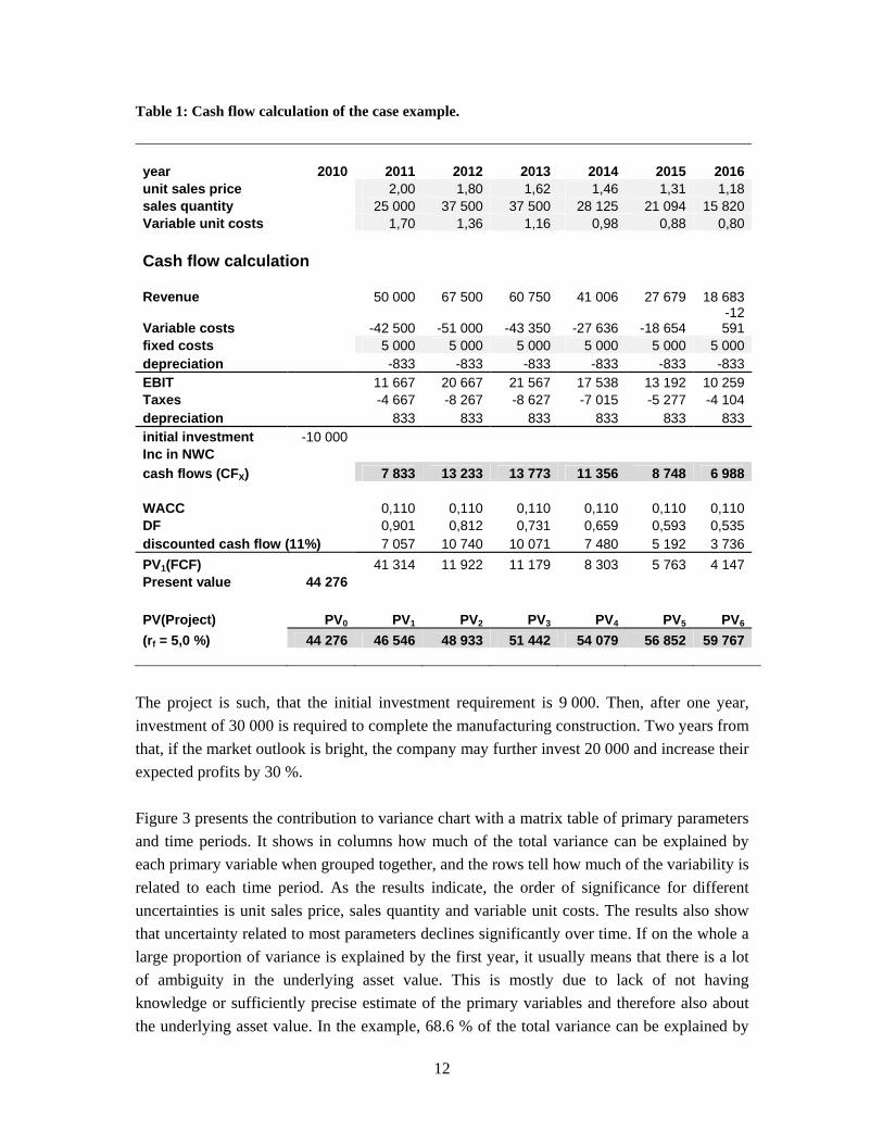
Table 1: Cash flow calculation of the case example.

year 2010 2011 2012 2013 2014 2015 2016unit sales price 2,00 1,80 1,62 1,46 1,31 1,18sales quantity 25 000 37 500 37 500 28 125 21 094 15 820Variable unit costs 1,70 1,36 1,16 0,98 0,88 0,80

Cash flow calculation Revenue 50 000 67 500 60 750 41 006 27 679 18 683

Variable costs -42 500 -51 000 -43 350 -27 636 -18 654 -12 591

fixed costs 5 000 5 000 5 000 5 000 5 000 5 000depreciation -833 -833 -833 -833 -833 -833EBIT 11 667 20 667 21 567 17 538 13 192 10 259Taxes -4 667 -8 267 -8 627 -7 015 -5 277 -4 104depreciation 833 833 833 833 833 833initial investment -10 000 Inc in NWC

cash flows (CFX) 7 833 13 233 13 773 11 356 8 748 6 988 WACC 0,110 0,110 0,110 0,110 0,110 0,110DF 0,901 0,812 0,731 0,659 0,593 0,535discounted cash flow (11%) 7 057 10 740 10 071 7 480 5 192 3 736

PV1(FCF) 41 314 11 922 11 179 8 303 5 763 4 147Present value 44 276

PV(Project) PV0 PV1 PV2 PV3 PV4 PV5 PV6

(rf = 5,0 %) 44 276 46 546 48 933 51 442 54 079 56 852 59 767

The project is such, that the initial investment requirement is 9 000. Then, after one year,

investment of 30 000 is required to complete the manufacturing construction. Two years from

that, if the market outlook is bright, the company may further invest 20 000 and increase their

expected profits by 30 %.

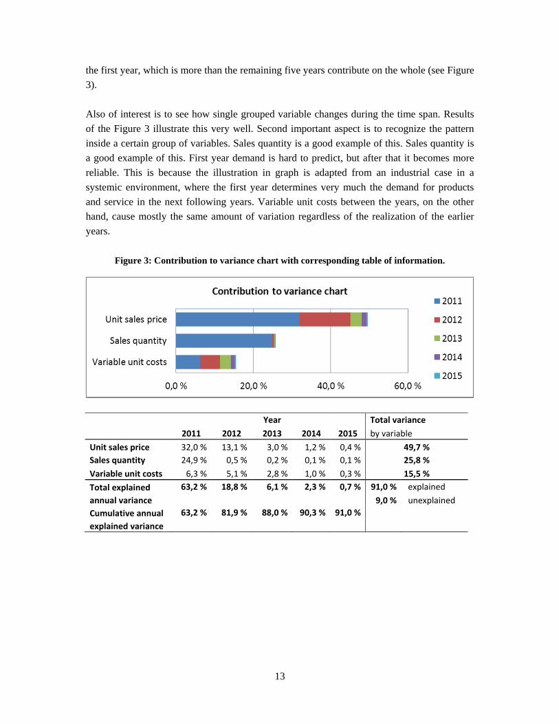
Figure 3 presents the contribution to variance chart with a matrix table of primary parameters

and time periods. It shows in columns how much of the total variance can be explained by

each primary variable when grouped together, and the rows tell how much of the variability is

related to each time period. As the results indicate, the order of significance for different

uncertainties is unit sales price, sales quantity and variable unit costs. The results also show

that uncertainty related to most parameters declines significantly over time. If on the whole a

large proportion of variance is explained by the first year, it usually means that there is a lot

of ambiguity in the underlying asset value. This is mostly due to lack of not having

knowledge or sufficiently precise estimate of the primary variables and therefore also about

the underlying asset value. In the example, 68.6 % of the total variance can be explained by

13

the first year, which is more than the remaining five years contribute on the whole (see Figure

3).

Also of interest is to see how single grouped variable changes during the time span. Results

of the Figure 3 illustrate this very well. Second important aspect is to recognize the pattern

inside a certain group of variables. Sales quantity is a good example of this. Sales quantity is

a good example of this. First year demand is hard to predict, but after that it becomes more

reliable. This is because the illustration in graph is adapted from an industrial case in a

systemic environment, where the first year determines very much the demand for products

and service in the next following years. Variable unit costs between the years, on the other

hand, cause mostly the same amount of variation regardless of the realization of the earlier

years.

Figure 3: Contribution to variance chart with corresponding table of information.

         Year        Total variance 

   2011  2012  2013  2014  2015  by variable 

Unit sales price  32,0 %  13,1 %  3,0 % 1,2 % 0,4 %  49,7 % 

Sales quantity  24,9 %  0,5 %  0,2 % 0,1 % 0,1 %  25,8 % 

Variable unit costs  6,3 %  5,1 %  2,8 % 1,0 % 0,3 %  15,5 % 

Total explained  63,2 %  18,8 %  6,1 % 2,3 % 0,7 %  91,0 %   explained 

annual variance                 9,0 %   unexplained 

Cumulative annual  63,2 %  81,9 %  88,0 % 90,3 % 91,0 %       

explained variance                      

14

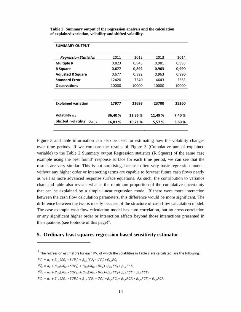
Table 2: Summary output of the regression analysis and the calculation of explained variation, volatility and shifted volatility.

SUMMARY OUTPUT             

              

Regression Statistics  2011 2012 2013 2014 

Multiple R  0,823 0,945 0,981 0,995 

R Square  0,677 0,892 0,963 0,990 

Adjusted R Square  0,677 0,892 0,963 0,990 

Standard Error  12420 7540 4643 2563 

Observations  10000 10000 10000 10000 

              

              

Explained variation  17977 21698 23700 25260 

              

Volatility i  36,40 % 22,35 % 11,49 % 7,40 % 

Shifted volatility dd,i 16,83 % 10,71 % 5,57 % 3,60 % 

              

Figure 3 and table information can also be used for estimating how the volatility changes

over time periods. If we compare the results of Figure 3 (Cumulative annual explained

variable) to the Table 2 Summary output Regression statistics (R Square) of the same case

example using the best found2 response surface for each time period, we can see that the

results are very similar. This is not surprising, because often very basic regression models

without any higher order or interacting terms are capable to forecast future cash flows nearly

as well as more advanced response surface equations. As such, the contribution to variance

chart and table also reveals what is the minimum proportion of the cumulative uncertainty

that can be explained by a simple linear regression model. If there were more interaction

between the cash flow calculation parameters, this difference would be more significant. The

difference between the two is mostly because of the structure of cash flow calculation model.

The case example cash flow calculation model has auto-correlation, but no cross correlation

or any significant higher order or interaction effects beyond those interactions presented in

the equations (see footnote of this page)3.

5. Ordinary least squares regression based sensitivity estimator

 3 The regression estimators for each PVx of which the volatilities in Table 2 are calculated, are the following:

, ∗ , ∗ ,

, ∗ , ∗ , ,

, ∗ , ∗ , , + ,

, ∗ , ∗ , , + , ,  

15

First consideration is how much the expected underlying asset value changes as a result of a

change in a primary cash flow calculation input parameter. However, the problem is that the

change in the input parameter is likely to change the uncertainty as well. It is also more likely

that larger values have larger absolute deviations from the mean than smaller values, while

the relative proportion of standard deviation in comparison with expected value is likely to

decrease. Therefore, sensitivity analysis has to take into account the effect of both the

expected value and the deviation change on the underlying asset value.

It would have been possible to use the exact form of (see the footnotes on the previous page).

However, to illustrate the method use, only the simple form of linear regression is applied

instead of the more advanced (but only slightly) more accurate response surface equations.

The use of approach is illustrated for the first year of cash flow calculation.

After the cash flow simulation, the regression model with most significant primary variables

is made to predict the underlying asset values. Independent variables in this case are the

Demand, Sales price and Variable costs in time period one. The dependent variable is present

value of the cash flows. Linear regression estimator results into the following equation for the

expected mean value of the underlying asset value:

9327 1.282 ∗ 55393 ∗51123 ∗

(3)

Because of the nature of the risk-neutral assumption in valuation, the expected underlying

asset value increases by risk-free interest rate between the time periods.

After that, simulation data is sorted according to the dependent variable (PV) estimator from

smallest to largest. Then the difference between the regression estimator values and the

simulation based realized values PV1 is calculated. The standard deviation of these

differences is 13 419, the same result which is also confirmed by regression software as

standard error. However, this average does not tell whether the standard deviation is the same

for large and small values expected values of the underlying asset. Therefore, the standard

deviation of the differences between simulated values and regression estimator values are

computed as a moving average consisting of 200 data points (-100…100) around each

estimated value. The results in the case example illustrate that the standard deviation

increases as a result of increase in expected value both for the standard deviation in time

period T1 and for the terminal value underlying asset distribution at the maturity Te. Linear

regression estimators result into the following equations for the standard deviations in T1 and

in Te

7535 0.0972 ∗ (4)

16

9675 0.0972 ∗ (5)

It is also possible to explain the standard deviations using the primary variables as

explanatory parameters instead of using combined regression estimator based expected mean

value of the underlying asset. This is suggested if such model has better explanatory power or

if it reveals some other property in the behavior of the underlying asset cash flow model, for

example as a result of significant non-linearity or heteroscedasticity caused only by a single

or few of the explanatory variables.

If the standard deviations of the underlying asset process at certain time points are known, it

is possible to compute the average volatility for each time period. Starting from the beginning

of the process, volatility i for each time period can be calculated according to Equation (6):

1 ∑

(6)

When the regression estimators are done, and they can be used for parameterizing common

option valuation methods, and especially their stochastic process parameters. In case of

several interacting options, this means usually choosing a lattice valuation approach. As a

result, we can finally check how real option value changes as a result of the change in its

primary cash flow calculation input parameter.

6. Results

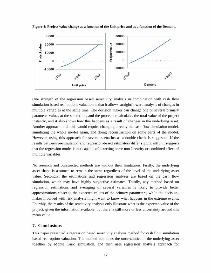
Figure 4 shows how the project value with real options changes as a result of change in unit

price (on the left) and Demand (on the right). The results and their linearity in this particular

case example are not very surprising. Increase in both cases in mostly due to the increase in

the underlying asset value as a result of the increase in the primary variable4. Also the options

contribute to the total value, but because they are of opposite types (option to abandon like a

put option and the extension option like a call option), they are valuable at opposite

situations. Therefore their combined added value does not change the rather linear nature of

the change in project value as a result of a change in a primary variable.

4 Next revision of this paper will include more detailed analysis of how much this change is caused by a change in 1) expected value, 2) volatility, and 3) by their combined interaction. 

17

Figure 4: Project value change as a function of the Unit price and as a function of the Demand.

One strength of the regression based sensitivity analysis in combination with cash flow

simulation based real options valuation is that it allows straightforward analysis of changes in

multiple variables at the same time. The decision maker can change one or several primary

parameter values at the same time, and the procedure calculates the total value of the project

instantly, and it also shows how this happens as a result of changes in the underlying asset.

Another approach to do this would require changing directly the cash flow simulation model,

simulating the whole model again, and doing reconstruction on some parts of the model.

However, using this approach for several scenarios as a double-check is suggested. If the

results between re-simulation and regression-based estimators differ significantly, it suggests

that the regression model is not capable of detecting some non-linearity or combined effect of

multiple variables.

No research and constructed methods are without their limitations. Firstly, the underlying

asset shape is assumed to remain the same regardless of the level of the underlying asset

value. Secondly, the estimations and regression analyses are based on the cash flow

simulation, which may have highly subjective estimates. Thirdly, any method based on

regression estimations and averaging of several variables is likely to provide better

approximations closer to the expected values of the primary parameters, while the decision-

maker involved with risk analysis might want to know what happens in the extreme events.

Fourthly, the results of the sensitivity analysis only illustrate what is the expected value of the

project, given the information available, but there is still more or less uncertainty around this

mean value.

7. Conclusions

This paper presented a regression based sensitivity analysis method for cash flow simulation

based real option valuation. The method combines the uncertainties in the underlying asset

together by Monte Carlo simulation, and then uses regression analysis approach for

18

estimating how a change in a primary cash flow variable – selling price, unit cost etc. -

affects simultaneously to the underlying asset properties - expected value, volatility, and

ambiguity - and as a result, via these indirect variables, changes the value of the project with

real options. The method allows changing of several primary variables at the same time, and

it calculates their combined effect on the project value instantly without need to re-

simulations. However, critical interpretation of the sensitivity analysis results is required

because of the limitations related to the use of regression model and partly subjective

estimates in cash flow simulation.

References

Birnbaum, Z. (1969). On the importance of different components in a multi-component

system. In Krishnaiah, P. (ed.) Multivariate analysis – II. New York, Academic Press.

Brandão, L., Dyer, J. & Hahn, W. (2005). Response to Comments on Brandão et al. (2005). Decision Analysis, Vol. 2, No. 2, June 2005, pp. 103-109. Campolongo, F., Saltelli, A., Sorensen, T., Tarantola, S. (2000). Hitchhiker’s guide to sensitivity analysis. In Sensitivity Analysis, (eds. Saltelli, A., Chan, K., Scott, E.) Wiley & Sons. pp. 15-47. Carriere, J. (1996). Valuation of early-exercise price of options using simulations and nonparametric regression. Insurance: Mathematics and Economics. Vol. 19, pp. 19-30. Copeland, T. & Antikarov, V. (2001). Real Options: A Practitioner’s Guide. Texere. Copeland, T. & Antikarov, V. (2005). Real options: meeting the Georgetown Challenge. Journal of Applied Corporate finance, Vol 17, no 2., pp 32-51. Cox, J., Ross, S. & Rubinstein, M. (1979). Option Pricing: A Simplified Approach. Journal of Financial Economics, No. 7, pp. 229-263. Coyle, D., Buxton, M., O’Brien, B. (2003). Measures of importance for economic analysis based on decision modeling. Journal of Clinical Epidemiology. Vol. 56, pp. 989–997. Cullen, A., Frey, H. (1999). Probabilistic Techniques in Exposure Assessment. Plenum Press: New York. Godinho, P. (2006). Monte Carlo Estimation of Project Volatility for Real Options Analysis. Journal of Applied Finance, Vol. 16, No. 1, Spring/Summer 2006.

19

Haahtela, T. (2006). Extended Binomial Tree Valuation when the Underlying Asset Distribution is Shifted Lognormal with Higher Moments. 10th Annual International Conference on Real Options, 14-17 June, New York, USA Haahtela, T. (2010). Recombining trinomial tree for real option valuation with changing volatility. 14th Annual International Conference on Real Options, 16-19 June, Rome, Italy. Haahtela, T. (2011). Estimating Changing Volatility in Cash Flow Simulation Based Real Option Valuation with Regression Sum of Squares Error Method. Presented in 15th Annual International Conference on Real Options, 15-18 June, Turku, Finland. Paper available in SSRN and in www.realoptionvaluation.com. Hahn, W. (2005). A Discrete-Time Approach for Valuing Real Options with Underlying Mean-Reverting Stochastic Processes. Dissertation, The University of Texas at Austin, May 2005 Hamby, D. (1994). A Review of techniques for parameter sensitivity analysis of environmental models. Environmental monitoring and assessment, Vol. 32, pp. 135-154. Helton, J., Davis, F. (2000) Sampling-based methods. In Sensitivity Analysis,( eds. Saltelli, A., Chan, K., Scott, E.) Wiley & Sons. pp. 101-153. uncertainty and sensitivity analysis. Risk Analysis, Vol. 22, No. 3, pp. 591–622. Helton, J,, Davis, F. (2002) Illustration of sampling-based methods for uncertainty and sensitivity analysis. Risk Analysis, Vol. 22, No. 3, pp. 591–622. Helton, J., Johnson, J., Sallaberry, C., Storline, C. (2006). Survey of sampling-based methods for uncertainty and sensitivity analysis. Reliability engineering and system safety. Vol. 91, pp. 1175-1209. Herath, H.. & Park, C. (2002). Multi-stage capital investment opportunities as compound real options. The Engineering Economist, Vol. 47, No.1, pp. 1-27. Hull, J. (1997). Options, Futures, and Other Derivatives. Prentice Hall, Third Edition. Iman, R., Helton, J. (1988). Investigation of uncertainty and sensitivity analysis techniques for computer models. Risk Analysis, Vol. 8, pp. 71-90. Kleijnen, J., Helton, J. (1999). Statistical analyses of scatterplots to identify important factors in large-scale simulations, 1: review and comparison of techniques. Reliability Engineering and System Safety. Vol. 65, No. 2, pp. 147–185.

20

Longstaff, F. & Schwartz, E. (2001). Valuing American options by simulation: A simple least-squares approach. Review of Financial Studies, Vol. 14, No. 1, pp. 113–147. Manache, G., Melching, C. (2008). Identification of reliable regression- and correlation-based sensitivity measures for importance ranking of water-quality model parameters. Environmental modelling & Software, Vol 23, pp. 549-562. Mun, J. (2002). Real Options Analysis: Tools and Techniques for Valuing Investments and Decisions. John Wiley & Sons, New Jersey, USA Rubinstein, M. (1983). Displaced diffusion option pricing. Journal of Finance, Vol. 38, No.1, March 1983, pp. 213-217. Saltelli, A., Tarantola, S., Campolongo, F., Ratto, M. (2004). Sensitivity analysis in practice. A Guide to Accessing scientific models. John Wiley & Sons, West Sussex, England. Saltelli, A., Andres, t., Homma, T. (1995). Sensitivity analysis of model output: performance ot the iterated fractional factorial design method. Computational Statistics and Data Analysis.Vol. 20, pp.387-407. Saltelli, A., Ratto, M., Andres, T., Campolongo, F., Cariboni, J., Gatelli, D., Saisana, M., Tarantola, S. (2008). Global sensitivity analysis. The primer. John Wiley & Sons. Samuelsson, P., (1965). Proof that properly anticipated prices fluctuate randomly. Industrial Management Review, Spring 1965, pp. 41-49. Smith, J. (2005) Alternative Approaches for Solving Real-Options Problems (Comments on Brandão et al. 2005). Decision Analysis, Vol. 2, No. 2, June 2005, pp. 89–102. Trigeorgis, L. (1993). The nature of option interactions and the valuation of investments with multiple real options. Journal of Financial Quantitative Analysis, Vo. 28, No 1, pp. 1-20. Turanyi, T. (1990). Sensitivity analysis of complex kinetic systems. Tools and applications. Journal of Mathematical Chemistry, Vol. 5, pp. 203-248. Yeh, K., Tung, Y. (1993). Uncertainty and sensitivity analyses of pit migration model. Journal of Hydraulic Engineering, ASCE 119 (2), pp. 262-283.