Information Asymmetry and Investment-Cash Flow Sensitivity

Asli Ascioglu Bryant University

Department of Finance (401) 232-6873

e-mail: ascioglu@leonardo.bryant.edu

Shantaram P. Hegde University of Connecticut Department of Finance

(860)-486-5135 e-mail: shantaram@business.uconn.edu

John B. McDermott* Fairfield University

Department of Finance (203)-254-4000 X2830

e-mail: jmcdermott@mail.fairfield.edu

ABSTRACT

Models of capital market imperfections predict that information asymmetry increases the sensitivity of a firm�s investment expenditures to fluctuations in internal funds by making external capital more costly. Previous empirical tests of the link between investment and financing decisions have relied on indirect measures of the degree to which a firm becomes financially constrained due to market frictions. In contrast, we use more direct measures of informational frictions derived from the market microstructure literature. Consistent with the theoretical prediction, our analysis shows that the scaled investment expenditures of firms with greater informed trade have greater investment- cash flows sensitivity. Our results are robust to multiple alternative measures of informed trade and liquidity.

PRELIMINARY DRAFT DO NOT QUOTE WITHOUT PERMISSION

NOVEMBER 2005

1. Investment � Cash Flow Sensitivity

In the pioneering work of Modigliani and Miller (1958) the financing and investment decisions of the firm

can be considered independent in the absence of market frictions. Many studies of information asymmetry

and capital market imperfections show that market frictions make external financing more costly than

internal financing because the former contains a �lemons� premium (e.g., Myers and Majluf (1984))1. In

this environment, Fazzari, Hubbard, and Petersen (1988) argue that the investment decision of firms that

nearly exhaust all their low-cost internal funds (i.e., have low dividend payout ratios) would be more

sensitive to fluctuations in their cash flows as compared with firms that pay high dividends. Holding

constant the investment opportunities of a firm, a reduction in internal funds would reduce capital

expenditures by firms facing information costs. They observe �If information problems in capital markets

lead to financing constraints on investment, they should be most evident for the classes of firms that retain

most of their income. If internal and external finance are nearly perfect substitutes, however, then retention

practices should reveal little about investment by the firm. Firms would simply use external finance to

smooth investment when internal finance fluctuates,� (p. 164).

To test the predicted link between investment and financing, Fazzari et. al. classify firms with low-dividend

payouts as �most financially constrained� while those with high dividend payouts as �least constrained�

firms. They argue that the �most constrained� firms should have investment expenditures that are more

sensitive to internal cash flows and stock of liquidity then the �least constrained� firms. Their empirical

tests show substantially higher sensitivity of investment to cash flow and liquidity for firms that retain

nearly all of their income.

Kaplan and Zingales (1997) criticize Fazzari et al.�s classification procedure by pointing out that a firm�s

dividend policy is a choice variable, hence firms that choose to pay low dividends even though they could

pay out more are not necessarily financially constrained. For example, firms may raise dividends in

response to a reduction in personal dividend income tax rates. Using qualitative and quantitative

information from financial statements and reports, they identify firms as �never constrained� if they have

more funds than needed to finance their investment and as �likely constrained� if they are without access to

more funds than needed to finance their capital expenditures. In contrast to Fazzari et al., their findings

indicate that the investments of �likely constrained� firms are less sensitive to cash flows than the

investments of �never constrained� firms. Kaplan and Zingales (2000) also point out that we would not

expect investment cash-flow sensitivities to be a good measure of financing constraints. As Moyen (2004)

demonstrates with simulated data, it is hard to identify firms with financing constraints, and the investment-

cash flow sensitivity critically hinges on the classification procedure used. While some methods of

financial constraint identification show low sensitivity between investments and cash flows, others show

just the opposite.

Since a very important root cause of firms� financial constraints and higher external capital costs is

information asymmetry between firms and uninformed investors, we use measures of asymmetric

information derived from the market microstructure literature to classify firms as more or less financially

constrained. Following previous theoretical work, we assume firms have private information about their

investment opportunities. Informed investors invest in gathering info about firms� prospects and trade on

that information, but the uninformed investors do not. Studies by Demsetz (1968), Copeland and Galai

(1983), Glosten and Milgrom (1985), Kyle (1985), Glosten and Harris (1988), Fialkowski and Petersen

(1994), Bessimbinder and Kaufman (1997), Easley, Hvidkjaer, and O�Hara (2002), and Easley and O�Hara

(2004) indicate that measures of market liquidity (e.g., effective spread and price impact of trade measures)

and probability of informed trading (e.g., PIN) serve to capture information asymmetry between informed

and uninformed investors. That is the higher the liquidity costs, the more expensive is external financing as

compared to internal financing. Therefore, we argue that firms with higher effective spreads, greater price

impact of trades, and higher probability of informed trade are likely to rely more on internal cash flows and

internally generated capital for investment spending than firms with lower effective spreads and PIN.

Since we use a more direct measure of capital market frictions and of financing constraint, our

classification procedure better addresses the Kaplan and Zingales (1997) criticism of Fazzari et al.

Our research also seeks to bridge the gap between the existing but largely distinct literature on investment

in the corporate finance literature and liquidity in the market microstructure literature. A recent paper by

Easley and O�Hara (2004) makes clear the link between information and the cost of capital. Recently,

notable scholars in the microstructure literature (e.g., Madhavan (2004) and O�Hara (2003)) have suggested

that the microstructure literature must show economic meaning to become more relevant. Our study is a

modest step in that direction � specifically, linking liquidity in general and adverse selection in particular to

the investment decision of the firm.

2. Data and Methodology

2.1. Sample Selection

Our original data set is the 1,224 firms of Standard and Poor�s 1500 (S&P 1500) with revenues greater than

$10,000,000 in 2000. The S&P 1500 is a well-known representative market index. Of the 1,224 firms in

the original sample, 509 firms satisfy the following selection criteria:

(a) Accounting data available in Standard and Poor�s COMPUSTAT to form the variables

necessary for our study.

(b) Data available in Center for Research in Securities Prices (CRSP) daily master file

(c) Transactions data for January through June 2000 is available in the NYSE Transactions and

Quote (TAQ) database.

(d) Firm�s equity was traded on New York Stock Exchange (NYSE) or American Stock

Exchange (AMEX) for the entire period January to June 2000 inclusive.

(e) Fiscal year-end in June or later.

(f) Firm is not in the financial services industry.

The exclusion of NASDAQ firms is to ensure that our results are not driven by and to minimize the noise

due to the very different market structures. Further, the transaction-based models that we employ to

measure adverse selection are developed theoretically in a specialist (not dealer) market. The exclusion of

financial services industry firs in study of investment cash-flow sensitivities s standard practice in this

literature (e.g. Fazzari et. al (1988), Kaplan and Zingales (1997, 2000).

2.2. Data Sources

The Center for Research in Security Prices (CRSP) daily master file is used to calculate average daily

volume, price, and return volatility. The NYSE TAQ database is used to obtain empirical estimates of our

transaction data based liquidity measures.

We use the first 6 months of year 2000 quotes and trades from TAQ data. In using the TAQ data we apply

the following filters which are standard in the study of transactions data:

a) Only BBO eligible primary market quotes are retained. (NYSE quotes�if it is a NYSE listed

stock, AMEX quotes if it is a AMEX listed stock)

b) Quotes and trades that have time stamp between 9:30 am to 4:00 p.m. are included.

c) Use quotations at least 15 seconds before the trade when we calculate trade execution costs

d) Use contemporaneous quotations for trade indicator identification. (See Bessembinder (2002))

e) Trade price must be > 0

f) Ask price must be > bid price must be > 0

g) Eliminate trades and quotes when trade price, ask quote, and bid quote that are lower (higher) than

7.5 standard deviations of the daily variation.

h) Keep trades with value of correction code is zero or one.

i) Exclude re-opening quotes.

2.3. Descriptive Statistics

Descriptive data on the final sample of 509 firms are presented in Table 1. As expected, the firms are large

but do vary greatly in size, volume, and spreads. The mean (median) market value is $8.89 billion ($1.87

billion). The mean (median) daily trading volume is 888,744 (362,062) shares. The mean (median) of

daily average trade weighted quoted half-spread is 7.49 cents (6.88 cents). The average (median) share

price is $34.17 ($28.00).

2.4. Empirical Measures of Liquidity and Adverse Selection

We use various well-established measures of liquidity from the microstructure literature in our study to

ensure the robustness of our results. Specifically, we use: relative effective spread, the Glosten and Harris

(GH) (1988) and Huang and Stoll (HS) (1996) price impact of trade measures, and the Easley, Kiefer,

O�Hara, and Paperman (EKOP) (1996) probability of informed trade measure. In this section, we discuss

the estimation of each measure in turn.

2.4.1. Relative Quoted and Effective Spreads

We measure the relative quoted spread as the difference of the bid and ask quotes scaled by the quote mid-

point. It is well established that the quoted spread overestimates the cost of transacting, as it does not

account for trades that occur at prices inside the quotes. For example, Fialkowski and Petersen (1994)

observe that for most orders executed on the New York Stock Exchange the effective spread paid by

investors averages half the quoted spread. Thus, we calculate the relative effective spread as follows:

t

tt

MMP

SpreadEffective−

= *2 , (1)

where Pt is the transaction price and Mt is the midpoint of the matched quote. Quotes are matched to the

nearest (but not later) contemporaneous trade as suggested by Bessimbinder (2002).

2.4.2. Glosten and Harris (1988) Price Impact of a Trade

The Glosten and Harris (1988) price formation model assumes that order flow is uncorrelated through time.

They show the change in transaction prices (∆pt) can be written as

[ ] ,1 ttttt QQqp εψλ +−+=∆ − (2)

where qt is signed order flow in shares, λ is the variable (i.e., adverse selection) cost of a transacting, Qt and

Qt-1 are trade indicator variables, ψ measures the fixed cost of transacting, and εt is a zero mean disturbance

term that reflects price changes due to the arrival of public information. We use the Lee and Ready (1991)

algorithm is used to sign order flow (qt) and trade indicator variables (Qt) as modified by Bessembinder

(2002). Specifically, each trade is matched to its contemporaneous quote. If the trade takes place at above

the quote midpoint it is classified as a buy (i.e., Qt =+1), if the trade occurs below the prevailing quote

midpoint it is classified as a sell (i.e., Qt =-1). If the trade occurs at the quote midpoint, it is signed

according to the last price change; that is, Qt =1 if the last price change was positive and vice versa. The

signed order flow (qt) is the size of the trade multiplied by the trade indicator variable (Qt). The liquidity

parameters (λGH) for each firm are estimated by ordinary least squares using equation (2) with a constant

term added for misspecification. For each firm, we multiply λGH by the average trade size in shares (n) and

scale by the average daily closing price of a share. Thus, λGH *n / P represents the relative price impact of

the average trade of a firm�s stock or alternatively the adverse selection component of the relative effective

spread.

2.4.3. Huang and Stoll (1996) Price Impact of a Trade

We follow Huang and Stoll (1995) as well as Bessembinder and Kaufman (1997) to decompose the

effective spread into its transitory and permanent components. Uniformed trades result in a transitory

change in transaction prices (i.e., price reversal), while information-motivated trades lead to a permanent

price change. The realized spread (or price reversal) measures market maker revenue net of information

costs. It is defined for each trade as

),(2 τ+−= ttt VPQSpreadalizedRe (3)

where Qt is the trade indicator variable, Pt is the transaction price, and V t+ τ is the post-trade value of the

security at some time in the future. To empirically estimate this measure of transactions costs, a proxy for

post-trade value is needed as well as a way to classify trades. The transaction price for the first trade at

least 5 minutes later (i.e., τ ≥ 5) is used as a proxy for the post-trade value.2 As in the Glosten-Harris

estimation, trades are signed using the Lee and Ready (1991) algorithm as modified by Bessembinder

(2002). The difference between the effective spread and realized spread scaled by the trade price provides

an estimate of the relative price impact or information content of a trade. Specifically,

,/)(2 tttt PMPQImpactPrice Relative −= +τ (4)

where Mt is the prevailing quote midpoint. In our empirical analysis we set τ equal to (at least) 5 minutes.

We omit trades (rather than use the first trade of the next trading day) for which there is no later trade in the

same day that permits the calculation of our trading cost measures.

2.4.4. Probability of Informed Trade

We estimate the probability of informed trading (PIN) using the model of Easley, Kiefer, O�Hara, and

Paperman (1996). Their model is a sequential trade model that estimates the level of informed trading

based on the order imbalance between buy and sell orders on any given day over a certain time period. The

intuition behind the EKOP model is that order imbalance increases among buy and sell orders when

informed traders are trading. The reason for that is the fact that informed traders take only one side of the

market depending on their information. Therefore, PIN estimation is based on the level of order

imbalances that are identified by the transaction data.

In the EKOP model, the probability of a news event is represented by α. A news event can be either a bad

news with a probability of δ, or good news with a probability of (1- δ). On any day, both liquidity trader

types (i.e., buyer and seller) arrive at a rate of ε. On the other hand, informed traders who know about the

news arrive only on days with news events with an arrival rate of µ. They buy if it is good news or sell if it

bad news. On days with informed trading, the imbalance of buys and sells is greater than the imbalance on

days without informed trading. Therefore, the estimation of the probability of informed trade is based on

the estimation of model parameters: α , µ , and ε . To obtain those parameters, we maximize the

following likelihood function:

!!)()1(

!)(

!!!)1()|,(

)(

)(

Se

Be

Se

Be

Se

BeSBL

SB

SBSB

εε+µδ−α+

ε+µεαδ+εεα−=θ

ε−ε+µ−

ε+µ−ε−ε−ε−

(5)

where B and S represent the number of buys and the number of sells on a given day, respectively. The

model assumes that days are independent, therefore the likelihood of observing the buys and sells over I

days, Iiii SBM 1),( == is the product of likelihoods:

∏=

=I

iii SBLML

1)|,()|( θθ . (6)

We maximize this likelihood function for each firm to find the estimates of the model parameters: α , µ ,

and ε . Then, the probability of informed trade (PIN) is calculated based on the estimated model

parameters as follows:

ε+αµαµ=

2PIN (7)

The numbers of buy orders and sell orders for each day are the only inputs required for the estimation of

PIN.3 Again, we use the Bessimbinder (2002) methodology to identify whether a trade is a buyer-initiated

or a seller-initiated.

2.5. Investment and Cash Flow Variables

We use COMPUSTAT data for 2000 to form the variables related to investment and cash flow used in our

analysis. The formation of the regression variables in our analysis is consistent with other empirical studies

of investment-cash flow sensitivities (e.g. Fazzari, Hubbard, and Petersen (1988), Kaplan and Zingales

(1997 and 2000)).

2.5.1. Investment Variables

Investment (I) in plant, property, and equipment comes from the COMPUSTAT data item for capital

expenditures. This data item includes expenditures for capital leases, funds for construction, and

reclassification of inventory to property. It excludes capital expenditures of discontinued operations,

changes due to foreign currency fluctuations, assets of acquired companies, and decreases in funds for

construction. We scale capital expenditures by the capital stock (K) taken as net plant, property, and

equipment at the beginning of the reporting year from COMPUSTAT. Thus, our scaled investment

variable is indicated as (I / K).

Tobin�s Q is a measure of the investment opportunity set that the firm faces. We use the Chung and Pruitt

(1994) measure of Q as follows:

( ) ,)(

)()()()()()(TABV

CABVCLBVINVBVLTDBVPSBVCSMVQ −++++= (6)

where MV(X) and BV(X) indicate the market and book variable of the argument X, respectively. CS is

common stock, PS is preferred stock, LTD is long-term debt, INV is inventory, CL is capital leases, CA is

current assets, and TA is total assets. The advantage of the Chung and Pruitt Q is the ease of computation

and the anticipated larger sample size as compared to when using other more complicated formulations of

Q. All variables for the computation of Q are taken from COMPUSTAT. We estimate Q as of the

beginning of the reporting year to capture the investment opportunity set the firm faces before the capital

investment is undertaken.

2.5.2. Cash Flow Variables

We use the COMPUSTAT data item for cash flow (CF), which is defined as income before extraordinary

items plus depreciation and amortization. As is customary in investment-cash flow sensitivity studies (e.g.,

Hubbard (1988), Moyen (2004)), we scale our measure of firm cash flow by net plant, property, and

equipment as of the beginning of the period from COMPUSTAT; our cash flow variable is thus denoted as

(CF / K).

3. Results and Analysis

3.1. Univariate Analysis

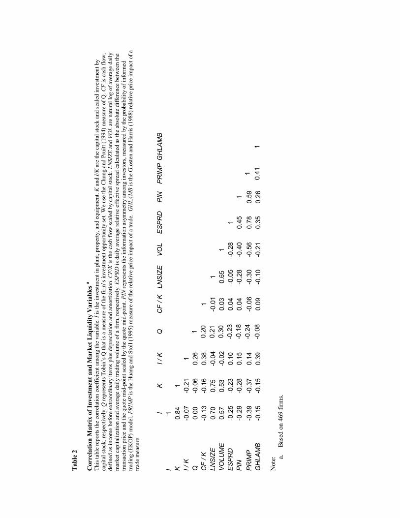
We begin with a univariate analysis of investment, cash flow, and market liquidity measures. Looking

down the column of Table 2 for scaled investment (I / K) we see positive correlation as expected with Q (ρ

= +0.26) and with scaled cash flow (ρ = 0.20) indicating that firms with a greater investment opportunity

set and greater cash flow invest in proportion to their capital stock. (I / K) has positive correlation (ρ ~

+0.14) with our liquidity measures such as relative effective spread, probability of informed trade, and our

price impact measures indicating that higher transaction and adverse selection costs are not associated with

lower scaled investment.. The liquidity measures, however, in general have negative correlations with

LNSIZE and Q. Also as expected, the liquidity measures have strong negative correlations with both

market value (LNSIZE) and trading volume (VOLUME) and LNSIZE and VOLUME are strongly positively

correlated indicating larger firms trade more often and have, in general, better liquidity. As would be

expected, our univariate analysis is exploratory and needs to be supplemented by a multivariate analysis

due to the complex interactions of the control and test variables used in our analysis..

3.2. Multivariate Analysis

In our multivariate analysis, we first investigate the effect of liquidity as measured by relative effective

spread on relationship the sensitivity of scaled investment (I / K) to scaled cashflow (CF / K). We then

extend our analysis to include the effect of liquidity on the firm�s cashflow-investment sensitivity using

price impact and PIN measures. Fazzari, Hubbard, and Petersen (1988) draw on the Q-model of investment

to investigate the investment-cash flow sensitivities of constrained versus unconstrained firms. We follow

he general framework of Fazzari et. al. as follows:

( ) ( ) itititit

KCFgKfK

I ε++=

X , (7)

where X represents a vector of variables theoretically motivated as determinants of investment. A linear

specification is motivated by the work of Summers (1981) and Hayashi (1982) by assuming a �quadratic

adjustment cost framework.� In addition to the value of Q at the beginning of each period, we add dummy

variables to capture the potential differences in scaled investment due to the differences in capital intensity

of industries and thus to avoid the bias caused by omitted explanatory variables. We also add LNSIZE,

which is defined as the natural log of the market value of equity as an explanatory variable to control for

potential differences in scaled investment due to the size of the firm. Moreover, larger (smaller) firms are

generally more (less) liquid, thus by adding LNSIZE as an explanatory variable for control for the

possibility that our liquidity partitions are proxies for firm size. Our variable of interest is a slope

differential dummy variable for the slope of the investment-cash flow sensitivity for firms with the greater

spreads or adverse selection costs. Specifically, we estimate the following cross-sectional specification

using ordinary least squares with the White (1980) covariance matrix:

( )( ) ,6431

*

87654

3210

iiiiii

iii

i

i

i

i

i

INDINDINDINDLNSIZE

QLIQDUMKCF

KCF

KI

εβββββ

βββα

+++++

++

+

+=

(8)

where LIQDUM i takes on the value of unity for the more illiquid firms in our sample as indicated by our

various liquidity measures , specifically the least liquid decile, and zero otherwise. Thus, the coefficient β2

captures the difference in cash flow-investment sensitivity for the most illiquid firms in our sample. If

internal and external capital are not perfect substitutes and spread serves to captures the transactions costs

associated with external financing, we hypothesize that firms with greater frictions (i.e., lower liquidity)

will have greater cash flow investment sensitivity (β2 > 0 ) than more liquid firms. Previous research

predicts (e.g. Hubbard (1998) and Kaplan and Zingales (1997)) we should expect to see a positive and

significant relationship between scaled investment and Q (β3 > 0) and also with scaled cash flow (β1 > 0).

If there are economies to firm size for investment, then β4 is expected to be greater than zero.

3.2.1. Analysis using Relative Effective Spread

If internal and external capital are not perfect substitutes, then transactions costs would be expected to

make equity capital more expensive as compared to internally generated funds. Fazzari, Hubbard, and

Petersen (1998) posit that this effect would be expected to be greater for �constrained� firms. Kaplan and

Zingales (1997 and 2000) counter with research to suggest greater investment-cash flow sensitivities are

not indicative of firms facing greater financing constraints. We posit that higher effective bid-ask spreads

serve to capture firms that are constrained, specifically due to asymmetric information problems. Amihud

and Mendelson (1988) and Brennan and Subrahmanyam (1996) demonstrated that firms with greater

adverse selection problems (and therefore greater spreads) will face a higher cost of capital (presumably for

externally sourced equity capital). This alone serves to make the difference between internal and external

capital more pronounced.

The variable LIQDUM is assigned a value of unity for firms with an average relative spread in the upper

decile of our sample and zero otherwise. We estimate equation (8) using the White (1980) covariance

matrix and present the results in Table 3. In Panel A of Table 3, we estimate the basic model of Fazzari,

Hubbard, and Petersen (1988) without the slope differential dummy for the investment-cash flow

sensitivity of illiquid firms. Regression #1 is estimated without the industry dummies and LNSIZE. As

expected the slope coefficient for Q is positive and highly significant (t = 7.83). The coefficient on scaled

cash flow (CF / K) is positive, as expected, and significant at the 5% level (t = 2.11). The adjusted R2 is

0.20. In regression #2, we add LNSIZE as an explanatory variable. The results for Q and (CF / K) do not

change materially; the coefficients have the same signs (positive as expected) and now are both highly

significant. The coefficient on LNSIZE is negative and significant (t = -2.11) indicating a diseconomy of

scale in investment. .In regression #3 we add the industry dummy variables4 but exclude firm size as

explanatory variables. The coefficient on Q remains positive and very highly significant and the coefficient

on (CF / K) remains positive but is now significant at the 1% level (t = 2.63) and the adjusted R2 increases

to 0.22 The results of estimating regression #3 suggest that there are industry effects in scaled investment

after controlling for Q and (CF / K). Specifically, Industry 3 (Transportation, Communications, and Public

Utilities) has significantly lower scaled investment and Industry 6 (Services) has significantly greater

scaled investment than Industry 2 (Construction and Manufacturing) in our sample period. In regression

#4, we now add LNSIZE back to the explanatory variables used in regression #3; the results remain

qualitatively similar. The exception being the sign on LNSIZE is negative as before but now insignificant (t

= 1.62).

In Panel B of Table 3, we add the slope differential dummy variable, LIQDUM, to capture the difference in

the investment-cash flow sensitivity of firms with the greatest relative effective spreads. In all four

regressions presented in Panel B, LIQDUM is positive indicating that the investment spending of firms

with the highest relative effective spreads are more sensitive to those with lower spreads, but do not meet

the 10% threshold for significance ( t ~ 1.45). The control variables are consistent with the regressions of

Panel A and are consistent with our expectations. Overall, the regressions in Panel B of Table 3 provide

weak support that the investment-cash flow sensitivities are greater for firms with greater relative effective

spreads. This highlights the need to use more refined measures of information asymmetry in our analysis.

3.2.2. Analysis using Glosten and Harris (GH) Measure of Relative Price Impact

Effective spread is a single and imperfect measure of liquidity. It is well-documented (e.g., Glosten and

Harris (1988), Glosten and Milgrom (1985), Copeland and Galai (1983), Kyle (1985)) in the microstructure

literature that the bid-ask spread has an adverse selection component to compensate market-makers for the

probability of dealing with better informed traders as well as a fixed component to cover order-processing

costs.5 The variable LIQDUMi is assigned a value of unity for firms with a GH price impact of trade

measure in the upper decile of our sample and zero otherwise. We then estimate equation (8) using the

White (1980) covariance matrix and present the results in Table 4. All four regressions in Table 4 have the

slope coefficient on LIQDUM as positive but not statistically significant (t ~ 0.85). The results for the

control variables are as expected with the estimated slope coefficients on Q and (CF/Q) are positive and at

least highly significant. The results presented in Table 4 also offer only weak support for the hypothesis

that firms with high adverse selection costs are likely to have greater investment cash-flow sensitivities. If

we accept that firms with greater adverse selection are more constrained, the results support Fazzari et. al

(1998) as compared to Kaplan and Zingales (1997, 2000). To supplement the analysis using the GH price

impact of a trade measure, we now turn to Huang and Stoll�s (1995) price impact of a trade measure.

3.2.3. Analysis using Huang and Stoll (HS) Measure of Price Impact of a Trade

The variable LIQDUMi is now assigned a value of unity for firms with a relative price impact of a trade in

the upper decile of our sample and zero otherwise and interacted with the scaled cash flow variable (CF/K).

We again estimate equation (8) using the White (1980) covariance matrix and present the Huang and Stoll

(1995) results in Table 5. All four regressions in Table 5 have the slope coefficient on LIQDUM as

positive and significant (t ~ 1.80) indicating that firms with trades that have the greatest relative price

impact (i.e., informed trade) as measured by HS have greater cash-flow investment sensitivities. This

provides confirmatory and statistically significant support for our hypothesis. Further, if we accept the

Fazzari et. al. (1988) that constrained firms will have greater investment cash-flow sensitivities than

unconstrained firms, then adverse selection is found to constrain the firm. If we accept Kaplan and

Zingales criticism of Fazzari, et. al., we can only say the firms with the greatest adverse selection as

measured by the price impact of a trade, causes its investment to be more sensitive to changes in cash-flow.

3.2.4. Analysis using EKOP Measure of Probability of Informed Trade

As a robustness check of our findings in the previous sub-section, we now repeat the analysis using a very

different microstructure measure of informed trade. Easley, Keifer, O�Hara, and Paperman (1996) provide

an empirically obtainable measure of the probability of informed trade (PIN) using transactions data. More

recently, Easley and O�Hara (2004) show that the cost of capital is higher for firms with a greater

probability of informed trade. Thus, we expect to find that firms with the highest probability of informed

trade, will have greater investment-cash flow sensitivity. To test this proposition, we compute the

probability of informed trade using the EKOP methodology. We form a dummy variable, LIQDUMi, that is

unity for firms in the upper decile of PIN values and zero otherwise. As before, we interact LIQDUMi with

(CF/ K)i. Thus, the slope coefficient β2 captures the difference in cash flow-investment sensitivity for firms

with the highest probability of informed trade as measured by the EKOP (1996) PIN measure. We

hypothesize that firms with greater adverse selection as measured by the probability of informed trade will

be have greater cash flow investment sensitivity (β2 > 0) than firms with a lower probability of informed

trade. We estimate equation (8) with the White (1980) covariance matrix and report the results in Table 6.

In all four Table 6 regressions, the coefficient (β2) that captures the difference in slope of the investment -

cash flow sensitivity for high PIN firms is positive and significant at the 5% level. The positive and

significant coefficients for β2 indicate greater investment-cash flow sensitivity for firms with the highest

probability of informed trade. This is consistent with our hypothesis that firms with lower liquidity will

have greater frictions in acquiring external financial capital thus their capital investment spending will be

more sensitive to changes in internally generated capital (i.e., cash flow). Further, the slope coefficients on

Q, and (CF/K) are positive as expected and very highly significant in all of the Table 6 regressions and the

adjusted R2s are approximately 0.30. The analysis of this section provides evidence that our findings with

respect to price impact of a trade are robust to an alternative measure of market liquidity.

4. Conclusions

To the extent that internal and external financing are not perfect substitutes, we expect and find a positive

relationship between capital investment spending and cash flow after controlling for the investment

opportunities of the firm. Further, for firms with the lowest liquidity (or highest adverse selection), the

difference between internal and external financing becomes more relevant due to a lemons problem. Thus,

we expect firms with lower liquidity to have greater investment - cash flow sensitivities. We use both an

indirect (effective spread) and direct measures (GH, HS, and PIN) of adverse selection to investigate this

potential and recognized important constraint on raising external capital and its effect on firm�s investment

� cash flow sensitivity. Consistent with our conjecture, we do find that the firms with the greatest informed

trade (i.e., lowest liquidity) in our large sample of NYSE firms have greater investment �cash flow

sensitivity. Our findings are robust to various measures of informed trade and liquidity, specifically

Huang and Stoll (1995) price impact of a trade and Easley, Kiefer, O�Hara, and Paperman�s (1998)

probability of informed trade. The results of our analysis using effective spread (a coarse measure of

adverse selection) and the Glosten-Harris price impact of a trade do not contradict our findings; we do find

results that are consistent but fail to rise to a conventional level of statistical significance.

If we accept a priori, that firms with greater adverse selection are more constrained, our findings support

those of Fazzari, Hubbard, and Petersen (1988) as compared to Kaplan and Zingales (1997 and 2000) in the

ongoing debate over whether investment � cash flow sensitivities are helpful in identifying firms that face

greater financial constraints. If we accept that Kaplan and Zingales (1997 and 2000) criticism of Fazzari et.

al,, we note simply that adverse selection is associated with the firm�s investment being more sensitive to

its internally generated cash flow. Thus, we find a role for adverse selection and liquidity in the firm�s

investment decision. Further, our findings are consistent with liquidity effect on the firm�s investment

decision as posited in Easley and O�Hara (2004) and also with Moyen (2004) who shows the investment

cash flow sensitivities are highly dependent on the method of classifying a firm as constrained or not.. Our

research represents a modest step in empirically establishing a direct link between market liquidity and the

investment decisions of the firm.

1 First by Akerlof (1970). 2 Bessembinder (1999) finds that using the quote mid-point for the post trade value yields essentially the same results. 3 We use Quant Optimization Method in GQOPT optimization package of FORTRAN to estimate PIN for each firm. 4 Industry classifications are based on two-digit SIC codes as in Bhushan (1989). Note the base case in all of our regressions involving industry dummies is industry 2 (construction and manufacturing). Note that industry 5 (finance, real estate, and insurance) is excluded from our sample. 5 Some theoretical models suggest an inventory component of the spread as well although the empirical support for inventory costs is weak (e.g., Madhavan and Smidt (1991)).

References Akerlof, G. A. (1970), �The Market for �Lemons�: Quality Uncertainty and the Market Mechanism,� Quarterly Journal of Economics, Vol. 84, No. 2, pp. 488-500. Amihud, Y. and H. Mendelson (1988), �Liquidity and Asset Prices: Financial Management Implications,� Financial Management, Spring, pp. 5-15. Bessimbinder, H. and H. M. Kaufman (1997), �A Comparison of Trade Execution Costs for NYSE and NASDAQ-Listed Stocks,� Journal of Financial and Quantitative Analysis, Vol. 32, No. 3, pp. 287-310. Bessembinder, H. (2002), �Issues in Assessing Trade Execution Costs,� Journal of Financial Markets, Vol. 6, No. 3, pp. 233-57 Benston, G. J. and R. L. Hagerman (1974), �Determinants of the Bid-Ask Spread in the Over-the-Counter Market,� Journal of Financial Economics, Vol. 1, No. 4, pp. 353-364. Bhushan, R. (1989), �Firm Characteristics and Analyst Following,� Journal of Accounting and Economics, Vol. 11, No. 2, pp. 255-274. Brennan, M. J. and A. Subrahmanyam (1996), �Market Microstructure and Asset Pricing: On the Compensation for Illiquidity in Stock Returns,� Journal of Financial Economics, Vol. 41, No. 3, pp. 441-464. Chung, K. H. and S. W. Pruitt (1994), �A Simple Approximation of Tobin�s Q,� Financial Management (Autumn), pp. 70-74. Copeland, T. C. and D. Galai (1983), �Information Effects on the Bid-Ask Spread,� Journal of Finance, Vol. 38, No. 5, pp 1457-1469. Demsetz, H. (1968), �The Cost of Transacting,� Quarterly Journal of Economics, Vol. 82, No. 1, pp.44-54. Easley, D., S. Hvidkjaer, and M. O�Hara (2002), �Is Information Risk a Determinant of Asset Returns?, Journal of Finance, Vol. 57, No. 5, pp. 2185-2221. Easley, D., N.M Kiefer, M. O�Hara, and J.B. Paperman (1996), �Liquidity, Information, and Infrequently Traded Stocks,� Journal of Finance, Vol. 51, pp. 1405-1436. Easley, D. and M. O�Hara (2004), �Information and the Cost of Capital,� Journal of Finance, Vol. 59, No. 4, pp. 1553-1583. Fazzari, S. M., Hubbard, R. G., and B. C. Petersen (1988), �Financing Constraints and Corporate Investment,� Brookings Papers on Economic Activity, No. 1, pp. 141-195. Fialkowski, D. and M. Petersen (1994), �Posted versus Effective Spreads: Good Prices or Bad Quotes?� Journal of Financial Economics, Vol. 35, No. 3, pp. 269-292. Glosten, L. R. and L. E. Harris (1988), �Estimating the Components of the Bid/Ask Spread,� Journal of Financial Economics, Vol. 21, No. 1, pp. 123-142. Glosten, L. R. and P. R. Milgrom (1985), �Bid, Ask, and Transaction Prices in a Specialist Market with Heterogeneously Informed Traders,� Journal of Financial Economics, Vol. 14, No. 1, pp. 71-100.

Hayashi, F. (1982), �Tobin�s Marginal q and Average q: A Neoclassical Interpretation,� Econometrica, Vol. 50, No. 1, pp. 213-224. Huang, R., and Stoll, H. 1996. Dealer versus Auction Markets: A Paired Comparison of Execution Costs on the NASDAQ and the NYSE. Journal of Financial Economics 41:313-357. Hubbard, R. G. (1998), �Capital-market Imperfections and Investment,� Journal of Economic Literature, Vol. 36, No. 1, pp. 193-225. Kaplan, S. N. and L. Zingales (1997), �Do Investment-cash flow Sensitivities Provide Useful Measures of Financing Constraints,� Quarterly Journal of Economics, Vol. 112, No. 1, pp. 169-215. Kaplan, S. N. and L. Zingales (2000), �Investment-cash flow Sensitivities are Not Valid Measures of Financing Constraints,� Quarterly Journal of Economics, Vol. 115, No. 3, pp. 707-712. Kyle, A. S. (1985), �Continuous Auctions and Insider Trading,� Econometrica, Vol. 53, No. 6, pp. 1315-1335. Lee, C.M.C. and M. J. Ready (1991), �Inferring Trade Direction from Intraday Data,� Journal of Finance, Vol. 46, No. 2, pp. 733-746. Madhavan, A. (2000), �Market Microstructure: A Survey,� Journal of Financial Markets, Vol. 3, No. 3, pp. 205-258. Madhavan, A. and S. Smidt (1991), �A Bayesian Model of Intraday Specialist Pricing,� Journal of Financial Economics, Vol. 30, No. 1, pp 99-134. Modigliani, F. and M. Miller (1958), �The Cost of Capital, Corporation Finance and the Theory of Investment,� American Economic Review, Vol. 57, No. 2, pp. 261-297. Moyen, N. (2004), �Investment-cash Flow Sensitivities: Constrained versus Unconstrained Firms,� Journal of Finance, Vol. 59, No. 5, pp. 2061-2092. Myers, S. C. and N. S. Majluf (1984), �Corporate Financing and Investment Decisions When Firms have Information that Investors Do Not Have,� Journal of Financial Economics, Vol. 13, No. 2, pp. 187-221. O�Hara, M. (1999), �Making Market Microstructure Matter,� Financial Management, Vol. 28, No. 2, pp 83-91. Summers, L. H. (1981), �Taxation and Corporate Investment: A q-Theory Approach,� Brookings Papers on Economic Activity, No. 1, pp. 67-127. White, H. (1980), �A Heteroscedasticity-Consistent Covariance Matrix Estimator and a Direct Test for Heteroscedasticity,� Econometrica, Vol. 48, No. 4, pp. 817-838.

Table 1

Descriptive Statistics for Sample of Non-Financial Service Industry, NYSE and AMEX-listed Firms in S&P 1500 Index for the period January 1, 2000 through June 30, 2000. Panel A: Descriptive Statistics for Final Sample Average

Closing Price ($)

Market Cap. ($000)

Daily NYSE Volume (Shares)

Dollar Quoted Half- Spread ($)

Relative Quoted Half- Spread (%)

(n=509 ) Mean 34.17 8,889,068 888,744 0.0749 0.3098 Median 28.00 1,873,688 362,062 0.0688 0.2467 Max. 510.26 277,717,76

920,257,390 0.5803 2.8643

Min. 2.81 43,464 9,895 0.0379 0.0726 Panel B: Distribution of Final Sample by Industry Codec Industry Code (Description) Number of

FirmsProportion of

Sample (n=509) IND1 (Mining) 33 0.06 IND2 (Construction and Manufacturing) 291 0.57 IND3 (Transportation, Communication, and Utilities) 87 0.17 IND4 (Wholesale and Retail Trade) 40 0.08 IND5 (Finance, Insurance, and Real Estate) 0 0.00 IND6 (Services) 58 0.11 Notes: a. S&P 1500 List obtained from Standard and Poor�s COMPUSTAT. b. Data for Panel A is obtained from CRSP Daily Master file with the exception of quote data, which is obtained from NYSE TAQ database. c. We follow Bhushan (1989) for industry classification. The industry groups are (1) Mining (two-digit SIC codes: 10-14), (2) Construction and Manufacturing (two-digit SIC codes: 15-39), (3) Transportation, Communication, and Public Utilities (two-digit SIC codes: 40-49), (4) Wholesale and Retail Trade (two-digit SIC codes: 50-59), (5) Finance, Insurance, and Real Estate (two-digit SIC codes: 60-67), and (6) Services (two-digit SIC codes: 70-96). Two-digit primary SIC codes are obtained from COMPUSTAT.

Tab

le 2

C

orre

latio

n M

atri

x of

Inve

stm

ent a

nd M

arke

t Liq

uidi

ty V

aria

bles

a Th

is ta

ble

repo

rts th

e co

rrel

atio

n co

effic

ient

am

ong

the

varia

ble.

I is t

he in

vest

men

t in

plan

t, pr

oper

ty, a

nd e

quip

men

t. K

and

I/K a

re th

e ca

pita

l sto

ck a

nd sc

aled

inve

stm

ent b

y ca

pita

l sto

ck, r

espe

ctiv

ely.

Q re

pres

ents

Tob

in�s

Q th

at is

a m

easu

re o

f the

firm

�s in

vest

men

t opp

ortu

nity

set

. We

use

the

Chun

g an

d Pr

uitt

(199

4) m

easu

re o

f Q. C

F is

cas

h flo

w,

defin

ed a

s inc

ome

befo

re e

xtra

ordi

nary

item

s plu

s dep

reci

atio

n an

d am

ortiz

atio

n. C

F/K

is th

e ca

sh fl

ow s

cale

d by

cap

ital s

tock

. LNS

IZE

and

VOL

are

natu

ral l

og o

f ave

rage

dai

ly

mar

ket c

apita

lizat

ion

and

aver

age

daily

trad

ing

volu

me

of a

firm

, res

pect

ivel

y. E

SPRD

is d

aily

ave

rage

rela

tive

effe

ctiv

e sp

read

cal

cula

ted

as th

e ab

solu

te d

iffer

ence

bet

wee

n th

e tra

nsac

tion

pric

e an

d th

e qu

ote

mid

-poi

nt sc

aled

by

the

quot

e m

id-p

oint

. PIN

repr

esen

ts th

e in

form

atio

n as

ymm

etry

am

ong

inve

stor

s, m

easu

red

by th

e pr

obab

ility

of i

nfor

med

tra

ding

(EK

OP)

mod

el. P

RIM

P is

the

Hua

ng a

nd S

toll

(199

5) m

easu

re o

f the

rela

tive

pric

e im

pact

of a

trad

e. G

HLA

MB

is th

e G

lost

en a

nd H

arris

(198

8) re

lativ

e pr

ice

impa

ct o

f a

trade

mea

sure

.

I K

I /

K

Q

CF

/ K

LNS

IZE

VO

L E

SP

RD

P

IN

P

RIM

P

GH

LAM

BI

1

K

0.

84

1

I / K

-0

.07

-0.2

1 1

Q

0.00

-0

.06

0.26

1

C

F / K

-0

.13

-0.1

6 0.

38

0.20

1

LNS

IZE

0.

70

0.75

-0

.04

0.21

-0

.01

1

VO

LUM

E

0.57

0.

53

-0.0

2 0.

30

0.03

0.

65

1

E

SP

RD

-0

.25

-0.2

3 0.

10

-0.2

3 0.

04

-0.0

5 -0

.28

1

PIN

-0

.29

-0.2

8 0.

15

-0.1

8 0.

04

-0.2

8 -0

.40

0.45

1

PR

IMP

-0

.39

-0.3

7 0.

14

-0.2

4 -0

.06

-0.3

0 -0

.56

0.78

0.

59

1

GH

LAM

B

-0.1

5 -0

.15

0.39

-0

.08

0.09

-0

.10

-0.2

1 0.

35

0.26

0.

41

1 N

ote:

a.

Base

d on

469

firm

s.

Table 3 Q Model of Investment using Relative Effective Spread as Liquidity Measure This table shows the cross-sectional regression results when scaled investment (I/K) is regressed against scaled cash flow (CF/K), a high spread dummy variable and control variables. Panel A shows the estimation results for the following regression:

( ) ( ),64

31

76

543210

iii

iiiii

i

i

i

INDIND

INDINDLNSIZEQKCF

KI

εββ

βββββα

++

+++++

+=

Panel B shows the estimation results for the following regression:

( ) ( ),6431

*

8765

43210

iiiii

iiii

i

i

i

i

i

INDINDINDIND

LNSIZEQSPRDDUMKCF

KCF

KI

εββββ

ββββα

++++

+++

+

+=

We hypothesize that firms with greater frictions as measured by relative effective spread will be have greater cash flow investment sensitivity (β2) than firms with lower spreads. Therefore, the slope coefficient β2 captures the difference in cash flow- investment sensitivity for firms with higher relative effective spreads in the above regression specification. The descriptions of the variables used are provided below: I/K: investment scaled by beginning of period capital stock CF/K : cash flow scaled by beginning of period capital stock Q: Tobin�s Q measured by Chung and Pruitt (1994) SPRDDUM: dummy variable that takes the value of unity for firms with an average relative effective spread in

the upper decile of our sample and zero otherwise. LNSIZE: natural log of average daily market capitalization. IND(i): dummy variables that represent firm�s industry based on two-digit SIC code of a firm. Panel A: OLS Regressions without Slope Dummy for High Spread Firms Dependent Variable: Scaled Investment (I / K)

Regression # (1)

(2)

(3) (4)

Constant 0.1076*** (7.83)

0.3139*** (3.08)

0.1148*** (6.22)

0.2702*** (2.79)

CF / K 0.0821** (2.11)

0.0800*** (2.88)

0.0708*** (2.63)

0.0705*** (2.63)

Q 0.0481*** (3.53)

0.0607*** (4.16)

0.0446*** (3.18)

0.0548*** (3.57)

LNSIZE

-0.0151** (-2.11)

-0.0116 (-1.62)

IND1

-0.0233 (-1.37)

-0.0187 (-1.10)

IND3

-0.0398** (-2.05)

-0.0308 (-1.50)

IND4

0.0267 (0.71)

0.0261 (0.70)

IND6

0.0725** (2.32)

0.0695** (2.26)

n 509 509 509 509 Adjusted R2 0.20 0.21 0.22 0.23

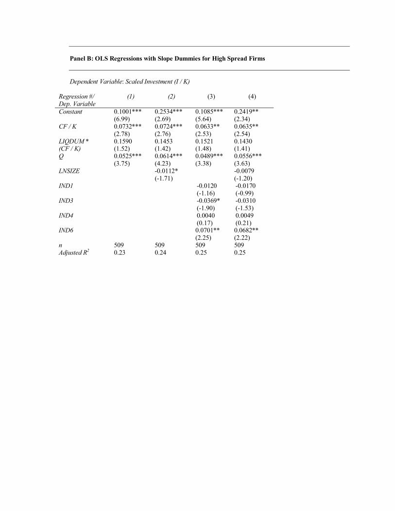
Panel B: OLS Regressions with Slope Dummies for High Spread Firms Dependent Variable: Scaled Investment (I / K)

Regression #/ Dep. Variable

(1) (2) (3) (4)

Constant 0.1001*** (6.99)

0.2534*** (2.69)

0.1085*** (5.64)

0.2419** (2.34)

CF / K

0.0732*** (2.78)

0.0724*** (2.76)

0.0633** (2.53)

0.0635** (2.54)

LIQDUM * (CF / K)

0.1590 (1.52)

0.1453 (1.42)

0.1521 (1.48)

0.1430 (1.41)

Q 0.0525*** (3.75)

0.0614*** (4.23)

0.0489*** (3.38)

0.0556*** (3.63)

LNSIZE

-0.0112* (-1.71)

-0.0079 (-1.20)

IND1

-0.0120 (-1.16)

-0.0170 (-0.99)

IND3

-0.0369* (-1.90)

-0.0310 (-1.53)

IND4

0.0040 (0.17)

0.0049 (0.21)

IND6

0.0701** (2.25)

0.0682** (2.22)

n 509 509 509 509 Adjusted R2 0.23 0.24 0.25 0.25

Table 4 Q Model of Investment using Glosten and Harris (1988) Price Impact Measure of Liquidity This table shows the cross-sectional regression estimation results when scaled investment (I/K) is regressed against scaled cash flow (CF/K), a high price impact dummy variable, and control variables as follows:

( ) ( ),6431

*

8765

43210

iiiii

iiii

i

i

i

i

i

INDINDINDIND

LNSIZEQLIQDUMKCF

KCF

KI

εββββ

ββββα

++++

+++

+

+=

We hypothesize that firms with greater adverse selection as measured by the price impact of a trade will have greater cash flow investment sensitivity (β2) than firms with lower price impacts. Therefore, in the above regression specification, the slope coefficient β2 captures the difference in cash flow- investment sensitivity for firms with a greater relative price impact of trading a single share of stock as Glosten and Harris (GH) (1988). The descriptions of the variables are provided below: I/K: investment scaled by beginning of period capital stock CF/K : cash flow scaled by beginning of period capital stock Q: Tobin�s Q measured by Chung and Pruitt (1994) LIQDUM: dummy variable that takes the value of unity for firms with relative GH price impact measure

in the upper decile of our sample and zero otherwise. LNSIZE: natural log of average daily market capitalization. IND(i): dummy variables that represent firm�s industry based on two-digit SIC code of a firm. Dependent Variable: Scaled Investment (I / K)

Regression #/ Dep. Variable

(1) (2) (3) (4)

Constant 0.1030*** (6.97)

0.2795*** ( 2.78)

0.1111*** ( 5.58)

0.2422** ( 2.53)

CF / K

0.0746*** ( 2.80)

0.0737*** ( 2.78)

0.0652** ( 2.57)

0.0654** ( 2.58)

LIQDUM * (CF / K)

0.1045 ( 0.96)

0.0924 ( 0.87)

0.0902 ( 0.84)

0.0820 ( 0.78)

Q 0.0514*** ( 3.68)

0.0617*** ( 4.19)

0.0476*** ( 3.28)

0.0559*** ( 3.60)

LNSIZE

-0.0129* (-1.85)

-0.0097 (-1.42)

IND1

-0.0220 (-1.26)

-0.0182 (-1.06)

IND3

-0.0384* (-1.94)

-0.0310 (-1.52)

IND4

0.0215 ( 0.70)

0.0214 ( 0.70)

IND6

0.0664** ( 2.07)

0.0644** ( 2.05)

n 509 509 509 509 Adjusted R2 0.22 0.22 0.23 0.24

Notes: a. t-ratios in parenthesis below parameter estimates computed using White (1980) covariance matrix. *, **, and ***denotes significance at the 10%, 5%, and 1% level, respectively.

Table 5 Q Model of Investment using Huang and Stoll (1995) Relative Price Impact Measure of Liquidity This table shows the cross-sectional regression estimation results when scaled investment (I/K) is regressed against scaled cash flow (CF/K), a high price impact dummy variable, and control variables as follows:

( ) ( ),6431

*

8765

43210

iiiii

iiii

i

i

i

i

i

INDINDINDIND

LNSIZEQLIQDUMKCF

KCF

KI

εββββ

ββββα

++++

+++

+

+=

We hypothesize that firms with greater adverse selection as measured by the probability of informed trade will have greater cash flow investment sensitivity (β2) than firms with a lower probability of informed trade. Therefore, in the above regression specification, the slope coefficient β2 captures the difference in cash flow- investment sensitivity for firms with a greater relative price impact of a trade as in Huang and Stoll (1995). The descriptions of the variables are provided below: I/K: investment scaled by beginning of period capital stock CF/K : cash flow scaled by beginning of period capital stock Q: Tobin�s Q measured by Chung and Pruitt (1994) LIQDUM: dummy variable that takes the value of unity for firms with a relative price impact measure

in the upper decile of our sample and zero otherwise. LNSIZE: natural log of average daily market capitalization. IND(i): dummy variables that represent firm�s industry based on two-digit SIC code of a firm. Dependent Variable: Scaled Investment (I / K)

Regression #/ Dep. Variable

(1) (2) (3) (4)

Constant 0.0984*** (6.94)

0.2150*** (2.18)

0.1065*** (5.54)

0.1843* (1.91)

CF / K

0.0721*** (2.84)

0.0716*** (2.82)

0.0638** (2.59)

0.0639*** (2.60)

LIQDUM * (CF / K)

0.2101* (1.94)

0.1966* (1.79)

0.1932* (1.78)

0.1848* (1.68)

Q 0.0522*** (3.82)

0.0590*** (4.12)

0.0488*** (3.44)

0.0537*** (3.56)

LNSIZE

-0.0085 (-1.24)

-0.0058 (-0.84)

IND1

-0.0182 (-1.06)

-0.0161 (-0.94)

IND3

-0.0345* (-1.76)

-0.0303 (-1.50)

IND4

0.0087 (0.34)

0.0092 (0.35)

IND6

0.0594* (1.92)

0.0585* (1.91)

n 509 509 509 509 Adjusted R2 0.25 0.25 0.26 0.26

Notes: a. t-ratios in parenthesis below parameter estimates computed using White (1980) covariance matrix. *, **, and ***denotes significance at the 10%, 5%, and 1% level, respectively.

Table 6 Q Model of Investment using Probability of Informed Trade as Liquidity Measure This table shows the cross-sectional regression estimation results when scaled investment (I/K) is regressed against scaled cash flow (CF/K), a high PIN dummy variable, and control variables as follows:

( ) ( ),6431

*

8765

43210

iiiii

iiii

i

i

i

i

i

INDINDINDIND

LNSIZEQLIQDUMKCF

KCF

KI

εββββ

ββββα

++++

+++

+

+=

We hypothesize that firms with greater adverse selection as measured by the probability of informed trade will have greater cash flow investment sensitivity (β2) than firms with a lower probability of informed trade. Therefore, in the above regression specification, the slope coefficient β2 captures the difference in cash flow- investment sensitivity for firms with a greater probability of informed trade as measured Easley, Kiefer, O�Hara, and Paperman (EKOP) (1996) PIN measure. The descriptions of the variables are provided below: I/K: investment scaled by beginning of period capital stock CF/K : cash flow scaled by beginning of period capital stock Q: Tobin�s Q measured by Chung and Pruitt (1994) LIQDUM: dummy variable that takes the value of unity for firms with a probability of informed trade (PIN)

in the upper decile of our sample and zero otherwise. LNSIZE: natural log of average daily market capitalization. IND(i): dummy variables that represent firm�s industry based on two-digit SIC code of a firm. Dependent Variable: Scaled Investment (I / K)

Regression #/ Dep. Variable

(1) (2) (3) (4)

Constant 0.1264*** (11.40)

0.3712*** (5.29)

0.1233*** (8.41)

0.3267*** (4.62)

CF / K

0.0621*** (2.77)

0.0595*** (2.62)

0.0503** (2.36)

0.0504*** (2.62)

LIQDUM * (CF / K)

0.2253** (2.47)

0.2107** (2.40)

0.2081** (2.29)

0.1983** (2.26)

Q 0.0424*** (3.52)

0.0549*** (4.05)

0.0351*** (3.03)

0.0460*** (3.40)

LNSIZE

-0.0191** (-3.67)

-0.0106*** (-2.78)

IND1

-0.0227 (-1.37)

-0.0159 (-0.97)

IND3

-0.0534*** (-4.47)

-0.0417*** (-3.26)

IND4

0.0145 (0.56)

0.0161 (0.62)

IND6

0.0710** (2.37)

0.0683** (2.30)

nb 486 486 486 486 Adjusted R2 0.27 0.30 0.31 0.32

Notes: a. t-ratios in parenthesis below parameter estimates computed using White (1980) covariance matrix. b. Sample reduced by 23 firms due to non-convergence of PIN estimation routine. *, **, and ***denotes significance at the 10%, 5%, and 1% level, respectively.