DEV 567: Project and Program Analysis

Lecture 6

Cash Flow, Sensitivity, Break-even Analysis and Simulation

2

Why Cash Flows? Cash flows, and not accounting

estimates, are used in project analysis because: They measure actual economic wealth. They occur at identifiable time points. They have identifiable directional flow. They are free of accounting definitional

problems.

3

The Meaning of RELEVANT Cash Flows.

A relevant cash flow is one which will change as a direct result of the decision about a project.

A relevant cash flow is one which will occur in the future. A cash flow incurred in the past is irrelevant. It is sunk.

A relevant cash flow is the difference in the firm’s cash flows with the project, and without the project.

4

Cash Flows: A Rose by Any Other Name Is Just as Sweet.

Relevant cash flows are also known as:-Marginal cash flows. Incremental cash flows. Changing cash flows.Project cash flows.

5

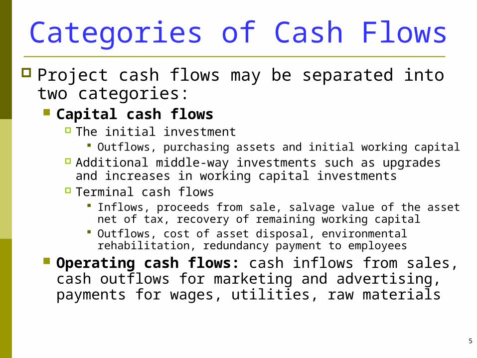
Categories of Cash Flows Project cash flows may be separated into

two categories: Capital cash flows

The initial investment Outflows, purchasing assets and initial working capital

Additional middle-way investments such as upgrades and increases in working capital investments

Terminal cash flows Inflows, proceeds from sale, salvage value of the asset net

of tax, recovery of remaining working capital Outflows, cost of asset disposal, environmental

rehabilitation, redundancy payment to employees Operating cash flows: cash inflows from sales,

cash outflows for marketing and advertising, payments for wages, utilities, raw materials

6

Essentials in Cash Flow Identification Principle of the stand-alone project

Evaluation of the proposed project purely on its own merits, in isolation from any other activities or the projects of the firm

Indirect of synergistic effects Negative effects, new model of car, lower sales of

existing model, must be deducted from future cash flows Positive effects, pharmacy adjacent to doctor’s clinic,

favorable impact on clinics cash flows to be added to pharmacy project’s cash flows

Opportunity cost principle: the most valuable alternative that is given up if the proposed investment project is undertaken Use of existing resources, space, building, rental value,

market value

7

Essentials in Cash Flow Identification Sunk cost, is an amount spent in the past in

relation to the project, but which cannot now be recovered or offset by the current decision Past consulting expenses

Overhead costs Utilities, executive salaries With or without the project, incremental costs to be

included Treatment of working capital

Current assets (inventories, accounts receivables) minus current liabilities (accounts, wages payable)

Increases in working capital is treated as cash outflows even though there is no actual cash outflow, opportunity cost

Capital flows, not operational flows, it is a fund

8

Essentials in Cash Flow Identification

After-tax cash flows Must be accounted for as a cash outflow, not

based on net cash flow but on taxable income Treatment of depreciation

Is not a cash flow In project appraisal, what is relevant is not the

accounting depreciation but tax allowable depreciation to measure the tax effect

Investment allowance, enhances NPV Financing flows, excluded. double

counting, included in the discount rate

9

Essentials in Cash Flow Identification Within-year timing of cash flows

Occurs at various points of time in a year Standard practice is to assume that capital expenditure

occur at the beginning of the year and all other cash flows occur at the end of the year

Points in cash flow timing is are set at the end of each year. An initial outlay of Tk. 50,000 at the start of year 1will be timed as occurring at the end of year zero.

Inflation and consistent treatment of cash flows and discount rates Nominal returns, incorporating the inflationary effect is

preferred over cash flow forecasts in real terms, excluding the inflationary effects

Fisher effect Consistency, cash flow in nominal terms- use nominal

discount rate; cash flow in real terms- use real discount rate

10

Project Cash Flows: Yes and No.

YES:- these are relevant cash flows:

Incremental future sales revenue. Incremental initial outlay. Incremental future salvage value. Incremental working capital outlay. Incremental future taxes.

11

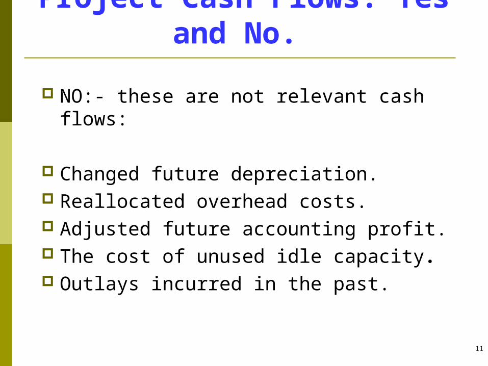
Project Cash Flows: Yes and No.

NO:- these are not relevant cash flows:

Changed future depreciation. Reallocated overhead costs. Adjusted future accounting profit. The cost of unused idle capacity. Outlays incurred in the past.

12

Cash Flows and Depreciation: Always a Problem.

Depreciation is NOT a cash flow. Depreciation is simply the accounting

amortization of an initial capital cost. Depreciation amounts are only

accounting journal entries. Depreciation is measured in project

analysis only because it reduces taxes.

13

Other Cash Flow Issues. Tax payable: if the project changes tax

liabilities, those changed taxes are a flow of the project.

Investment allowance: if a taxing authority offers this ‘extra depreciation’ concession, then its tax savings are included.

Financing flows: interest paid on debt, and dividends paid on equity, are NOT cash flows of the project.

14

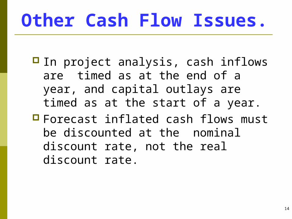
Other Cash Flow Issues.

In project analysis, cash inflows are timed as at the end of a year, and capital outlays are timed as at the start of a year.

Forecast inflated cash flows must be discounted at the nominal discount rate, not the real discount rate.

15

Using Cash Flows

All relevant project cash flows are set out in a table.The cash flow table usually reads across in End of Years, starting at EOY 0 (now) and ending at the project’s last year. The cash flow table usually reads down in cash flow elements, resulting in a Net Annual Cash Flow. This flow will have a positive or negative sign.

16

Delta Project Cash Flows Project start date 2001 Capital outlay in year 1 is $ 1 million; year 3 is

$0.5 million Economic life 8 years Working capital Y0-2000; Y1-2500; Y2-3100; Y3-

3600; Y4-4000; Y5-4300;Y6-4500; Y7-3000, Y8-0. Salvage value in Y8-$16,000 Depreciation on initial investment is 12.5% p.a.

upgrade depreciates @$100,000 for years 4-8. Sales forecasts After tax salvage value Accounting income Workbook 2.1

17

Asset expansion project cash flows

Initial investment Initial investment in plants and working capital

Net operating cash flows Add back depreciation Exclude depreciation from costs Add tax shield of depreciation (tax rate x

depreciation) Terminal cash flows

Proceeds from sale of assets minus taxes on sale of an assets plus recovery of working capital

18

Asset replacement project cash flows Initial investment

Initial investment in plants and working capital minus proceeds from sale of old asset plus taxes on sale of old assets

Incremental operating cash flows Operating cash flow of new assets minus

operating cash flow of old assets Terminal cash flow

Proceeds from sale of new asset- proceeds from sale of old asset - taxes on sale of old assets- taxes on sale of an assets-taxes on sale of old assets plus recovery of working capital

19

Project Cash Flows: Summary

Only future, incremental, cash flows are Relevant. Relevant Cash Flows are entered into a yearly cash flow table. Net Annual Cash Flows are discounted to give the project’s Net Present Value.

20

Overarching principles: We only need to estimate cash flows

that change as a result of accepting the project (incremental cash flows).

The amount of, and the timing of the cash flow must be estimated, not the

accounting profit/loss by ordinary accounting methods.

21

There are generally three kinds of cash flows that can be affected by a capital budgeting project:

1) Initial period cash flow2) Operating cash flow3) Terminal year cash flow

22

Since taxes are cash flows, we must include taxes in our cash flow estimates. All estimated cash

flows should be after-tax cash flow

estimates!

23

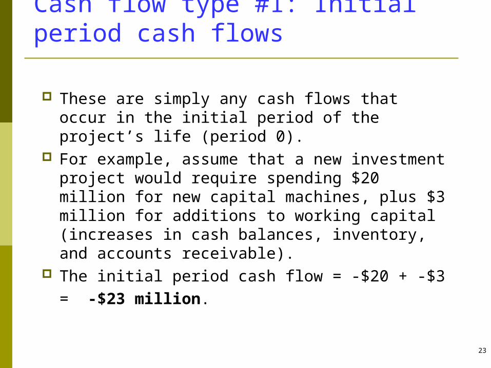
Cash flow type #1: Initial period cash flows

These are simply any cash flows that occur in the initial period of the project’s life (period 0).

For example, assume that a new investment project would require spending $20 million for new capital machines, plus $3 million for additions to working capital (increases in cash balances, inventory, and accounts receivable).

The initial period cash flow = -$20 + -$3= -$23 million.

24

Cash flow type #2: Operating cash flow

Accounting income for a period could be a measure of cash flow, except that depreciation (an expense, but not a cash flow) was subtracted in calculating it.

Operating cash flow equalsNet Income + Depreciation

25

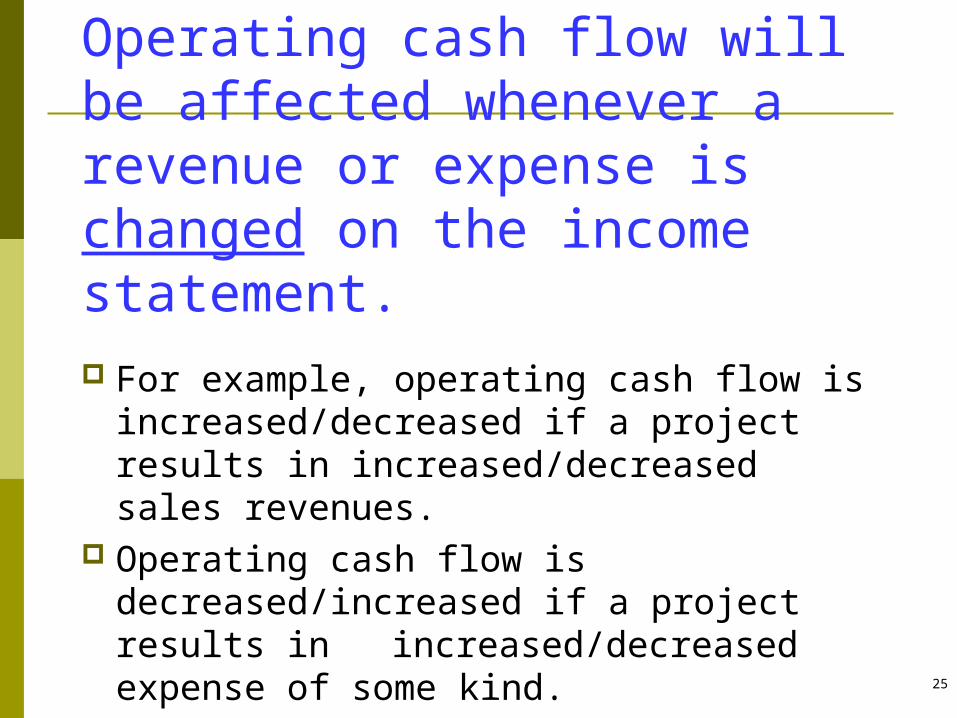
Operating cash flow will be affected whenever a revenue or expense is changed on the income statement. For example, operating cash flow is

increased/decreased if a project results in increased/decreased sales revenues.

Operating cash flow is decreased/increased if a project results in increased/decreased expense of some kind.

26

Continuing with the example project:

Assume the business currently has sales of $95 million and cash operating expenses of $65 million, plus $15 million of depreciation

expense. Assume the tax rate = 30%. Net income = ($95 - $65 - $15) x (1 - .3)

= $10.5 million. Operating cash flow = Net income +

depreciation = $10.5 + $15 = $25.5 million per year.

27

Assume that accepting the new investment project would increase the business sales by $10 million, and increase the operating costs by $4 million, plus increase depreciation expense by $2 million. What is the incremental operating cash flow for the project?

Class Exercise

28

Operating cash flow with the new project = ($105 - $69 - $17) x (1-.3) + $17 = $30.3 million. The incremental operating cash flow

for the project equals the change in cash flows from before accepting the project to after accepting it = $30.3 - $25.5 = $4.8 million per year. (Assume these benefits continue the same each year for 10 years.)

29

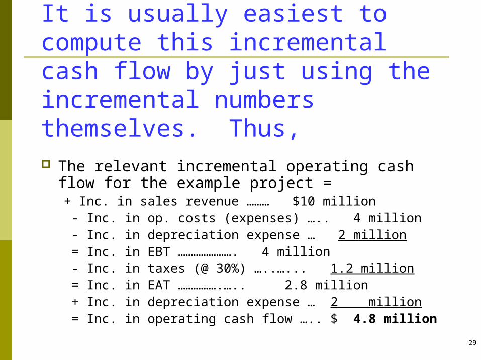
It is usually easiest to compute this incremental cash flow by just using the incremental numbers themselves. Thus, The relevant incremental operating cash flow

for the example project =+ Inc. in sales revenue ……… $10 million - Inc. in op. costs (expenses) ….. 4 million - Inc. in depreciation expense … 2 million = Inc. in EBT …………………. 4 million - Inc. in taxes (@ 30%) …..…... 1.2 million = Inc. in EAT …………….….. 2.8 million + Inc. in depreciation expense … 2 million = Inc. in operating cash flow ….. $ 4.8 million

30

Notice that this method of calculating the incremental operating cash flow requires you to simply identify every item in the company’s income statement that changes, and then to calculate the change in net income that results. Finally, the operating cash flow equals the change in net income plus the change in depreciation.

31

Cash flow type #3: Terminal year cash flows

These cash flows consist of any residual values (salvage values) recovered from the project at the end of its useful life.

For our example, assume that at the end of the project’s life, the machines could be sold to net $100,000 after taxes, and that the working capital ($3 million) is recovered in full.

Thus, the terminal year cash flow (year 10) for the project = $3.1 million.

32

The complete cash flows for the example project are:Periods:

0 1-10 10 - $23 + $ 4.8 + $ 3.1Assume that the cost of capital for the project equals 10%, the NPV is calculated to be $7.69 million.

33

Since the NPV > 0 we know the project is a good one.

We could alternatively have made the decision using the IRR method. IRR of the project can be calculated to be 17%. Since this is > the 10% cost of capital, the project should be accepted..

We could also have (alternatively) made the decision using the PI method. PI = 1.33, which is > 1.00.

34

Consider another example:

Assume the Widget Company is considering an investment to replace a production machine with a more efficient one.

Assume the new machine costs $100,000, and the old machine has a book value of $15,000 and a current salvage value of $25,000.

Assume the tax rate is 30%. What are the relevant cash flows for the project

analysis, and should the replacement be accepted?

Class Exercise 2

35

First, determine the initial period cash flows:

The $100,000 purchase price of the new machine is an immediate cash outflow.

The $25,000 salvage value of the old asset would be an immediate cash inflow.

Taxes on the gain from sale of the old asset is also an immediate cash outflow. Taxes = 30% x (SV-BV) = .3 x (25,000-15,000) = $3,000.

36

The total initial period (period 0) incremental cash flows for the replacement project are:

-$100,000 + $25,000 - $3,000 = -$78,000.

37

Next, we calculate the operating cash flows: Assume the new machine would reduce

operating costs by $35,000 per year for the next 8 years, compared to using the old machine. Depreciation expense would also increase by $12,500 per year for 8 years.

Net income will increase by ($35,000 - 12,500) x (1-.3) = $15,750.

Op. CF = Net Income + Depreciation = $15,750 + $12,500 = $28,250 per year, for 8 years.

Note that this is an annuity of benefits.

38

Assume that both the old machine and the new one would be fully depreciated after 8 years. With the new machine, sale in year 8 for

$5,000 => taxable gain on the sale equal to the salvage value minus the book value = ($5,000 – 0) = $5,000. Tax on this gain = $5,000 x .3 = $1,500.

With the old machine, sale in year 8 for $500 => taxable gain on the sale equal to the salvage value minus the book value = ($500 – 0) = $500.Tax on this gain = $500 x .3 = $150.

39

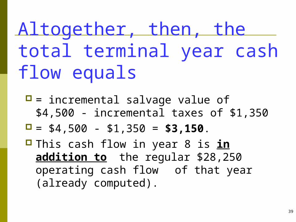
Altogether, then, the total terminal year cash flow equals

= incremental salvage value of $4,500 - incremental taxes of $1,350

= $4,500 - $1,350 = $3,150. This cash flow in year 8 is in addition

to the regular $28,250 operating cash flow of that year (already computed).

40

Important: While in general, any cash flow affected

by a project is relevant, we do not include any cash flows that are financing costs.

For example, we do not include interest expense or lease payments.

The reason for this is that all financial cash flows are implicitly included in the cost of capital used to find NPV (or used to compare to IRR). To include the

financial cash flows and then discount them to PV would be to double count their impact.

41

Project Analysis Under Risk

Incorporating risk into project analysis through adjustments to the discount rate, and by the certainty equivalent factor.

42

Introduction: What is Risk?

Risk is the variation of future expectations around an expected value.

Risk is measured as the range of variation around an expected value.

Risk and uncertainty are Interchangeable words.

43

Where Does Risk Occur?

In project analysis, risk is the variation in predicted future cash flows.

End of End of End of End of Year 0 Year 1 Year 2 Year 3

-$760 ? -$876 ? -$546 ?-$235 ? -$231 ? -$231 ?

-$1,257 $127 ? $186 ? $190 ?$489 ? $875 ? $327 ?$945 ? $984 ? $454 ?

Varying Cash FlowsForecast Estimates of

44

Handling Risk

Risk may be accounted for by evaluating the project using sensitivity and breakeven analysis.

Risk may be accounted for by (1) applying a discount rate commensurate with the riskiness of the cash flows, and (2), by using a certainty equivalent factor

There are several approaches to handling risk:

Risk may be accounted for by evaluating the project under simulated cash flow and discount rate scenarios.

45

Using a Risk Adjusted Discount Rate

The structure of the cash flow discounting mechanism for risk is:-

The $ amount used for a ‘risky cash flow’ is the expected dollar value for that time period.

A ‘risk adjusted rate’ is a discount rate calculated to include a risk premium. This rate is known as the RADR, the Risk Adjusted Discount Rate.

46

Defining a Risk Adjusted Discount Rate

Conceptually, a risk adjusted discount rate, k, has three components:-

1. A risk-free rate (r), to account for the time value of money

2. An average risk premium (u), to account for the firm’s business risk

3. An additional risk factor (a) , with a positive, zero, or negative value, to account for the risk differential between the project’s risk and the firms’ business risk.

47

Calculating a Risk Adjusted Discount Rate

A risky discount rate is conceptually definedas:

k = r + u + a

Unfortunately, k, is not easy to estimate. Two approaches to this problem are:1. Use the firm’s overall Weighted Average Cost of Capital, after tax, as k . The WACC is the overall rate of return required to satisfy all suppliers of capital.

2. A rate estimating (r + u) is obtained from the Capital Asset Pricing Model, and then a is added.

48

Calculating the WACC

Assume a firm has a capital structure of:50% common stock, 10% preferred stock, 40% long term debt.

Rates of return required by the holders of each are :common, 10%; preferred, 8%; pre-tax debt, 7%. The firm’s income tax rate is 30%.

WACC = (0.5 x 0.10) + (0.10 x 0.08) + (0.40 x (0.07x (1-0.30))) = 7.76% pa, after tax.

49

The Capital Asset Pricing Model This model establishes the covariance

between market returns and returns on a single security.

The covariance measure can be used to establish the risky rate of return, r, for a particular security, given expected market returns and the expected risk free rate.

50

Calculating r from the CAPM

The equation to calculate r, for a security with a calculated Beta is:

Where : is the required rate of return being calculated, is the risk free rate: is the Beta of the security, and is the expected return on the market.

rE ~fR

mR

51

Beta is the Slope of an Ordinary Least Squares Regression Line

Share Returns Regressed On Market Returns

-0.04

-0.02

0.00

0.02

0.04

0.06

0.08

0.10

0.12

-0.10 -0.05 0.00 0.05 0.10 0.15 0.20

Returns on Market, % pa

Ret

urn

s o

f S

har

e, %

p

a

52

The Regression Process

The value of Beta can be estimated as the regression coefficient of a simple regression model. The regression coefficient ‘a’ represents the intercept on the y-axis, and ‘b’ represents Beta, the slope of the regression line. 

itmtiit urbar  

Where,   = rate of return on individual firm i’s shares at time t = rate of return on market portfolio at time t = random error term (as defined in regression

analysis)

itrmtr

uit

53

The Certainty Equivalent Method: Adjusting the cash flows to their ‘certain’ equivalents

The Certainty Equivalent method adjusts the cash flows for risk, and then discounts these ‘certain’ cash flows at the risk free rate.

COetc

r

bCF

r

bCFNPV

22

11

11

Where: b is the ‘certainty coefficient’ (established by management, and is between 0 and 1); and r is the risk free rate.

54

Analysis Under Risk :Summary

Risk is the variation in future cash flows around a central expected value.

Risk can be accounted for by adjusting the NPV calculation discount rate: there are two methods – either the WACC, or the CAPM

Risk can also be accommodated via the Certainty Equivalent Method.

All methods require management judgment and experience.

55

People are generally risk-averse Simply looking at the expected value of the net present

value may not be enoughConsider a choice between two prizes, you canhave Tk. 100,000 for certain or a lottery ticket which will pay Tk. 200,000 with a probability of 0.5and Tk. 0 with a probability of 0.5, which one willyou choose?Please note that the two choices have the sameexpected value Certainty equivalent

An amount that would be accepted in lieu of achance to receive a possibly higher, but uncertain,amount.

Risk and Project Appraisal

56

Risk and Project Appraisal (Contd.)

A graphical illustration Risk aversion: decreasing marginal utility of wealth concave

function relating wealth and utility Risk neutral: constant marginal utility of wealth Risk lover: increasing marginal utility of wealth

Utility function

Consider two projects, A and B which have the followingPayoffs

2

1

)( WWU

State Probability Project A Project B

1 0.6 $100,000 $50,000

2 0.4 $0 $50,000

Expected value $60,000 $50,000

Expected utility 189.7 223.6

57

Risk and Project Appraisal (Contd.)

58

According to expected value criteria project A is preferred

E[UA] = 0.6*(100,0001/2)=189.7

E[UB] = 0.6*(50,0001/2)+0.4*(50,0001/2) =223.6

We can calculate the certainty equivalent of the twoprojectsFor project A, For Project B,U(CE) = 189.7 U(CE) = 223.6CE1/2= 189.7 CE1/2= 223.6CE = 36,000 CE = 50,000Because project B has the greater certainty equivalent, it isthe preferable projectIf people are risk neutral, then expected net present value willgive the right answer

Risk and CBA (Contd.)

59

Sensitivity Analysis

Analyzing project risks by making mechanical trial and error changes to forecast values of selected variables.

Analyzing the risks of investment projects, by changing the values of forecasted variables.

Finding the values of particular variables which give the project a Breakeven NPV of zero.

60

Process of Analysis

Identification of those variables which will have significant impacts on the NPV, if their future values vary around the forecast values.

The variables having significant impacts on the NPV are known as ‘sensitive variables’.

The variables are ranked in the order of their monetary impact on the NPV.

The most sensitive variables are further investigated by management.

61

Management Use of Sensitivity and Breakeven Analysis

Sensitive variables are investigated and managed in two ways:

(1) Ex ante; in the planning phase; more effort is used to create better forecasts of future values. If management decides the project is too risky, it is abandoned at this stage.

Using Sensitivity:

62

Management Use of Sensitivity and Breakeven Analysis

•(2) Ex post; in the project execution phase; management monitors the forecasted values. If the project is performing poorly, it is abandoned or sold off prior to its planned termination.

Using Sensitivity:Sensitive variables are investigated and managed in two ways:

63

Management Use of Sensitivity and Breakeven Analysis

Using Breakeven:

• Forecasted calculated Breakeven values of variables are continuously compared against actual outcomes during the execution phase.

64

Terminology Within the Analysis

Sensitivity and Breakeven analyses are also known as: ‘scenario analysis’, and ‘what-if analysis’.

Point values of forecasts are known as: ‘optimistic’, ‘most likely’, and ‘pessimistic’.

Respective calculated NPVs are known as: ‘best case’, ‘base case’ and ‘worst case’.

Variables giving a ‘breakeven’ value, return an NPV of zero for the project.

65

Steps in Sensitivity Analysis

Calculate the project’s NPV using the most likely value estimated for each variable

Select from the set of uncertain variables those which the management feels may have an important bearing on predicted project performance.

Forecast pessimistic, most likely, and optimistic values for each of these variables over the life of the project.

Recalculate the project’s NPV for each of these three levels of each variable. While each particular variable is stepped through each of its three values, all other variables are held at their most likely values.

Calculate the change in NPV for the pessimistic to optimistic range of each variable.

Identify sensitive variables.Important: Selection of appropriate variables, andestablishing valid upper and lower forecast values.

66

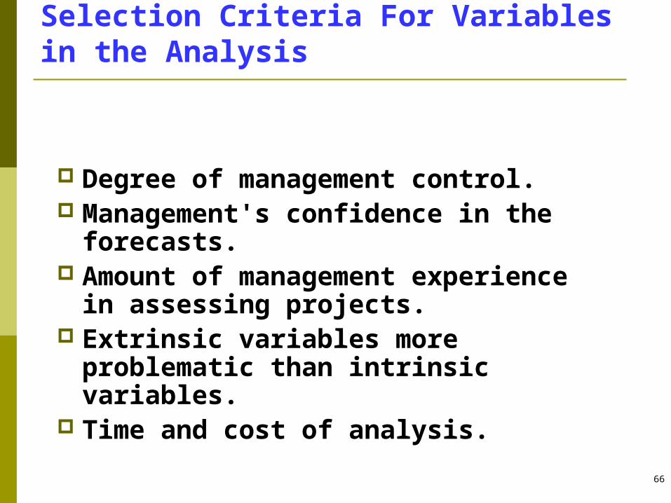
Selection Criteria For Variables in the Analysis

Degree of management control. Management's confidence in the

forecasts. Amount of management experience

in assessing projects. Extrinsic variables more

problematic than intrinsic variables.

Time and cost of analysis.

67

Real Life Examples Forecast Errors

Large blowouts in initial construction costs for Sydney Opera House, Montreal Olympic Stadium.

Big budget films are shunned by critics and public alike; e.g ‘Waterworld’: whilst cheap films become classics; eg.‘Easy Rider’.

High failure rate of rockets used to launch commercial satellites.

68

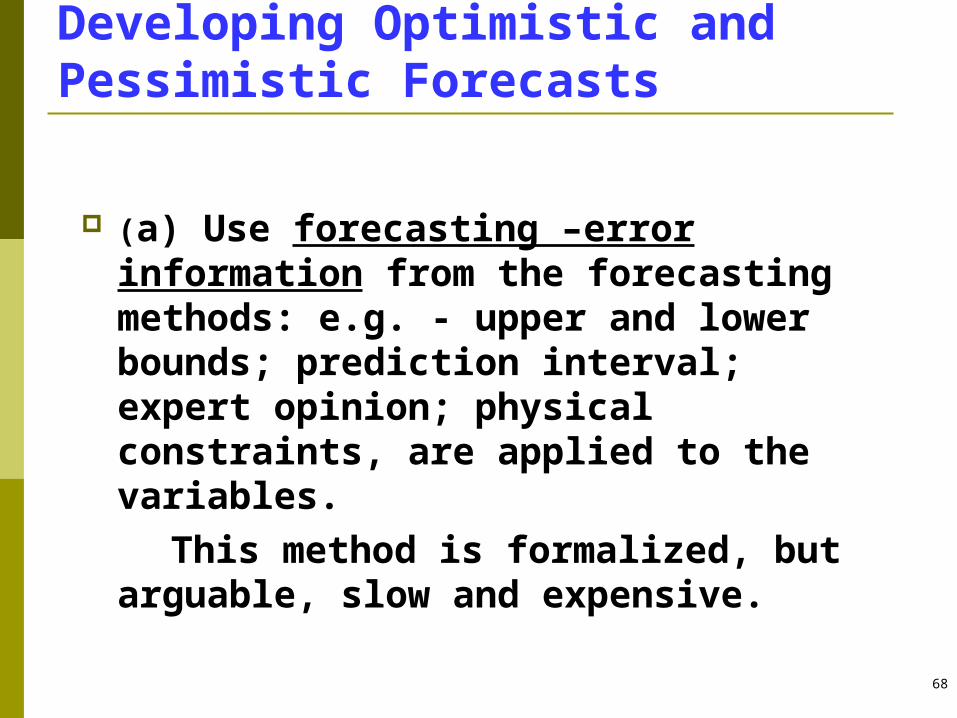
Developing Optimistic and Pessimistic Forecasts

(a) Use forecasting –error information from the forecasting methods: e.g. - upper and lower bounds; prediction interval; expert opinion; physical constraints, are applied to the variables.

This method is formalized, but arguable, slow and expensive.

69

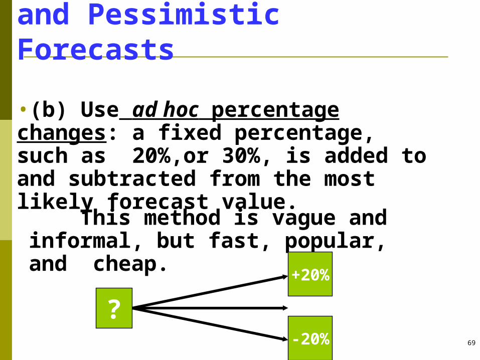
Developing Optimistic and Pessimistic Forecasts

•(b) Use ad hoc percentage changes: a fixed percentage, such as 20%,or 30%, is added to and subtracted from the most likely forecast value.

This method is vague and informal, but fast, popular, and cheap.

?

+20%

-20%

70

Sensitivity analysis example: Delta Project

Forecast Variable Value Variables for sensitivity analysis

Pessimistic Optimistic

Initial outlay $1,000,000 √ $1,200,000 $800,000

Upgrade cost(yr3) $500,000 X

Project life 8 years X

Working capitalAfter year 0

X

Salvage value $16,000 √ 0 $32,000

Tax depreciation rate

12.5% p.a. X

Sales volume 696,106+ 500,000Units p.a. after upgrade

√ Minus 1 SE of the regression,-16701 -20% (400,000)

Plus 1 SE of the regression, +16701+20%(600,000)

Selling price $0.50, 0.75 after five years

√ $0.30 $0.90

Production costs $0.10 per unit √ $0.13 $0.08

Other costs $50,000 p.a. $55,000 after 5 yr

√ $70,000 $35,000

Company tax rate 30% p.a. X

Required rate of return

5.37% p.a. √ 12% 4%

71

Delta Project: Sensitivity Analysis Results

Variable Sheet Number Pessimistic NPV Optimistic NPV Range

Initial outlay 2(1),(2) $856,208 $1,160,706 $304,498

Total asset salvage value 2(3),(4) $1,001,089 $1,015,825 $14,736

Regressed sales forecasts 2(5),(6) $972,600 $1,044,314 $71,714

Extra sales 2(7),(8) $869,480 $1,147,434 $277,954

Unit selling prices 2(9),(10) ($431,798) $2,379,109 $2,810,907

Unit production cost 2(11),(12) $870,393 $1,100,500 $230,107

Other costs 2(13),(14) $926,608 $1,082,594 $155,986

Required rate of return 2(15),(16) $427,220 $1,166,326 $739,106

72

Delta Project: Sensitivity Analysis Results

• Workbook 8.1

73

Sensitivity Analysis

Sensitivity analysis Partial sensitivity analysis Worst and best-case analysis

According to bridge supporters, the salvage value after 30 years will be $50 million. According to ferry supporters, the bridge will have zero salvage value after 30 years

Profile Cost Annual Benefit

Salvage value

NPV5% 10%

Bridge supporters

100 12 50 96.0 16

Ferry supporters

130 10 0 23.7 -35.7

74

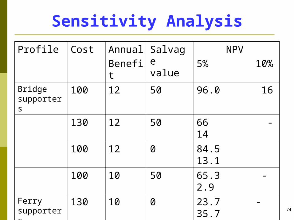
Sensitivity Analysis

Profile Cost Annual

BenefitSalvage value

NPV5% 10%

Bridge supporters

100 12 50 96.0 16

130 12 50 66 -14

100 12 0 84.5 13.1

100 10 50 65.3 -2.9Ferry supporters

130 10 0 23.7 -35.7

100 10 0 53.7 -5.7

130 12 0 54.5 -16.9

130 10 50 35.3 -32.9

75

Sensitivity Analysis

Carry out sensitivity analysis changing salvage value,e.g. plugging the bridge supporters salvage

value in ferry supporters profile the discount rate the construction costs annual benefit

Discount rate Construction cost from 130 to 100

Annual benefits from 10 to 12

Salvage value from 0 to 50

5% +30 +30.7 +11.5

10% +30 +18.9 +2.8

76

Break-even Analysis: Product Unit Price

Unit Price Project NPV

0.20 -1,089,2460.25 -760,5220.30 -431,7980.35 -152,6990.40 78,0410.45 308,1480.50 538,2540.55 768,3610.65 1,228,5750.70 1,458,6820.75 1,688,7890.80 1,918,8950.85 2,149,0020.90 2,379,1090.95 2,609,2161.00 2,839,323

Project NPV Versus Unit Selling Price

-1500

-1000

-500

0

500

1000

1500

2000

2500

3000

3500

0.00 0.50 1.00 1.50

Th

ou

san

ds

Unit Selling Price

Pro

ject

NP

V

77

Break-even Analysis: Required Rate of Return

Reqd Rate % Project NPV

4 $1,166,3265 $1,049,8526 $941,4077 $840,3528 $746,1039 $658,13010 $575,94711 $499,11212 $427,22013 $359,90014 $296,81415 $237,65216 $182,12717 $129,97818 $80,96419 $34,86520 -$8,52321 -$49,38822 -$87,902

Project NPV Versus Required Rate of Return

-500

-

500

1,000

1,500

0 10 20 30 40

Th

ou

san

ds

Required Rate of Return

NP

V in

Do

llars

78

Break-even Analysis: Unit Production Cost

Unit Cost Project NPV

0.08 1,100,2810.09 1,054,2730.10 1,008,2640.11 962,2560.12 916,2480.13 870,2400.14 824,2310.15 778,2230.16 732,2150.17 686,2070.18 640,1980.19 594,1900.20 548,182

Project NPV Versus Unit Production Cost

0

200

400

600

800

1,000

1,200

0.00 0.05 0.10 0.15 0.20 0.25

Thou

sand

s

Unit Production Cost: Dollars

Pro

ject

NP

V

79

Outputs and Uses

Each forecast value is entered into the model,and one solution is given.

Solutions can be summarized automatically, or individually by hand.

Variables are ranked in order of the monetary range of calculated NPVs.

Management investigates the sensitive variables.

More forecasting is done, or the project is accepted or rejected as is.

80

Strengths and Weaknesses of Analysis

Strengths: Easy to understand. Forces planning discipline. Helps to highlight risky variables. Relatively cheap.

Weaknesses Relatively unsophisticated. May not capture all information. Limited to one variable at a time. Ignores interdependencies.

81

Introduction

Project risk analysis by simultaneous adjustment of forecast values.

Simulation allows the repeated solution of an evaluation model.

Each solution randomly selects values from predetermined probability distributions.

All solutions are summarized into an overall distribution of NPV values.

This distribution shows management how risky the project is.

82

Simulation Terminology

The treatment of risk by using simulation is known as ‘stochastic’ modeling.

Other names for our term ‘Simulation’, are - ‘Risk Analysis’, ‘Venture Analysis’,’Risk Simulation’, ‘Monte Carlo Simulation’.

The name ‘Monte Carlo Simulation’ helps visualization of repeated spins of the roulette wheel, creating the selected values.

Each execution of the model is known as a ‘replication’ or ‘iteration’.

83

The Role of Simulation

Follows the initial creation and basic testing of the representative model.

Is sometimes used as a test of the model.

Emphasizes the need for formal forecasting, and requires close specification of the forecast variables.

Draws managements attention to the inherent risk in any project.

Focuses attention on accurate model building.

84

Probability Distributions of Forecast Variables

Uniform: upper and lower bounds required.

Triangular: pessimistic, most likely, and optimistic values required

Normal: mean and variance required.

Exponential: initial value and growth factor required.

85

Process of Computation per Replication

A value of a variable is selected from its distribution using a random number generator.

For example: Sales 90 units; selling price per unit $2,350; component cost per unit $1,100; labour cost per unit $280.

These values are incorporated into the model, and an NPV is calculated for this replication.

The NPV for this replication is stored, and later reported as one of many in an overall NPV distribution.

86

Making the Replications

Each replication is unique. Selection of values from the distribution is

made according to the particular distributions

The automated process is driven by a random number generator.

Excel add-ons such as ‘@Risk’ and ‘Insight’ can be used to streamline the process.

About 500 replications should give a good picture of the project’s risk.

87

Using the Output

Management can view the risk of the project.

Probability of generating an NPV between two given values can be calculated.

Probability of loss is the area to the left of a zero NPV.

88

Benefits and Costs of Simulation

Benefits Focuses on a detailed definition and analysis of risk. Sophisticated analysis clearly portrays the risk of a

project Gives the probability of a loss making project Allows simultaneous analysis of variables

Costs Requires a significant forecasting effort. Can be difficult to set up for computation. Output can be difficult to interpret.