IEPC-93-099 934

PREDICTION OF ELECTRIC THRUSTER LIFETIME

V. I. Baranov, A. I. Vasin, A. A. Kalyaev, V. A. Petrosov

The Scientific-Research Institute of Thermal Processes, Moscow, Russia

3. With the specified limiting admissible (critical)ABSTRACT value of erosion, the regression can be used to predict

lifetime.The prediction of lifetime is effected using the

nonlinear regressive dependence of the electric thruster I. Problems to be solvedaccelerating channel wall erosion on time. The originaldata are results of electric thruster lifetime tests that Based on such ideas, an application package waslasted up to 4000 hours. In calculation of the regression developed in the Pascal language to fit PC IBM AT. Itthe simplex and bootstrap methods are used as well as helps to solve the following problems.robust procedures. 1. Determination of parameters of erosion regressive

Using various acceleration coefficients which dependence on time.constitute lifetime-testing time ratios, the law of The basic data are values of accelerating channelpredicted lifetime distribution and lifetime parameters wall erosion at the corresponding instants of time thatwere defined together with confidence intervals for the were obtained during tests. Based on physical andprediction error. The results were obtained as the statistical pictures of the erosion development process,outcome of repeated statistical simulation using personal several kinds of approximating functions are chosen.computers. The present approach could be used in Due to nonlinearity of regressions, thus obtained, theirlifetime predictions based on other parameters of coefficients are defined using the simplex method, to bedegradation, more precise the method of deformed polyhedron.

To avoid errors in results of calculations due toINTRODUCTION possible overshoots and interferences during measure-

ments and their processing, the so called robust, i. e.To demonstrate and verify electric propulsion statistically stable, estimations of regression coefficients

lifetime in ground conditions by way of full life testing are used.will require much time. The bench running time of only Robust m'ethods are based on lessening the weight ofone engine, whichis equal to 4000 hours, can be obtained measurement data as they move away from thein the course of 1.5 year developmental tests with the distribution center. For this purpose in regressionaccount of necessary breaks of thruster operation coefficient calculations the robust functions of Huber,related to inspections, taking measurements, Hampel, Tukey and Andrews are used [1].maintenance work on test rigs, etc. But one testing is not The mathematical description of the algorithm forenough. That is why the full cycle of lifetime tests will the regression robust coefficients computation involvestake years of work and large expenditures, the following.

This can be avoided with the help of accelerated tests. Regression coefficients are found by the simplexTo determine the concept of such tests, to develop method.methods and procedures of tests and experimental data In the rocess, the objective functionprocessing an analysis of SPT-type electric thruster - 2 p(Xi) -* min,lifetime tests of 1500...4000 hours was made from which ithe following is inferred: wherep (x) - p (x);

1. As the parameter, determining lifetime, erosion of v (X),is the robustics function;the accelerating channel can be assumed which is Xi Yi - Y(2)defined by variation of insulator butt-end radial s 'dimensions. ,Y is the result of observation in the point ti;

2. The dependence of erosion on time is well Y(tt) is the regression value in the point tr;approximated by the nonlinear function regression, s is the robust estimate of the residual mean-that, in particular, allows to observe the dynamics of root-square deviation;erosion development.

1

935 IEPC-93-099

S med I Yi - Y (t) 1 2. Selection of such regression, which approximates0.6745 the experimental data best, from several alternative

functions.Fig. 1 illustrates the Tukey robustic function given The method is based on the calculation of regression

as an example. being performed using only a part of experimentalpoints. For the remaining points the quantity of their

Tukey Function deviation from the regression is defined. Further, theerror of adjustment is computed, representing the

S(r.()}, il ,a ,ix , difference of mean squares of these deviations and mean. I > a , .o0 squares of deviations from the regression for the points

for which the regression was computed. In doing so, thebootstrap and Jacknife procedures are used as well as

x ross verification [2 ]. In Table 1 are listed the formulae-a . a used for computing these criteria and the residual root-mean-square error.

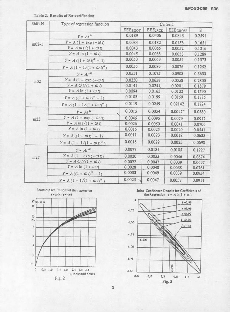
SResults of the abovementioned lifetime tests were" processed by this method. The calculation was

, performed for six kinds of the regression function.S. , ix Values of criteria are given in Table 2. Priority is given

fXl .- ' to functions with the least values of criteria. It is clearI.a' x a \that most often such functions are Y- A In ( + u )

Sand Y- + , t' the first one offers the advantage ofhaving no asymptote.

3.Determination of confidence intervals forregression.

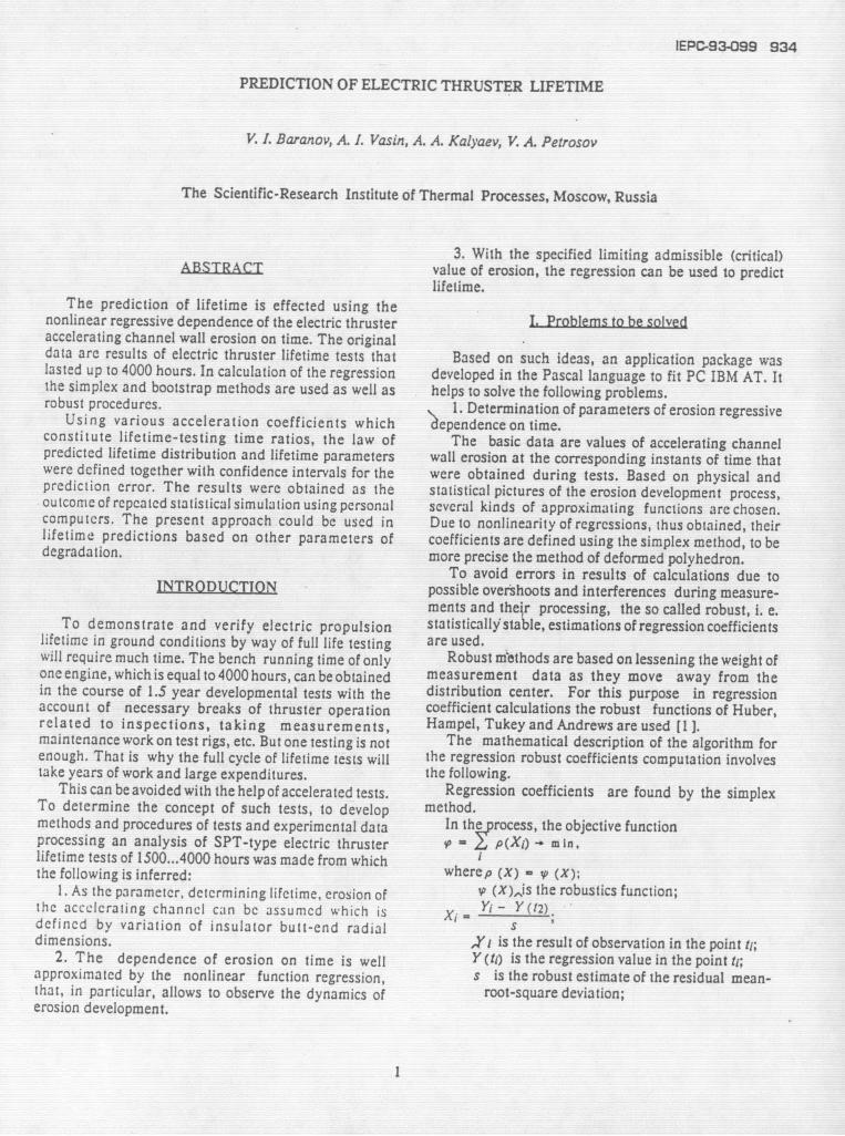
q/N A large number of bootstrap realizations for thetransformed regression equation are created(500... 1000). Fig. 2 shows some bootstrap realizations of

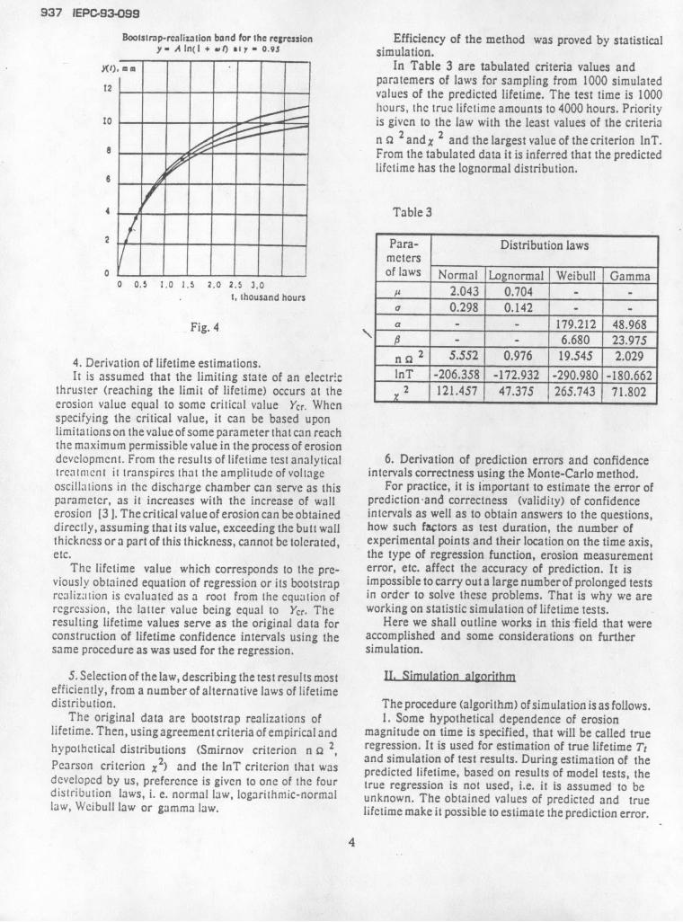
s the insulator wall erosion regressive dependence ontime. The bootstrap realizations are used as original datafor construction of various types of bootstrap-confidenceintervals accdrding to the bootstrap theory [2 ]. Besides,confidence intervals are obtained also without bootstrap,based on the coefficient-linearized regression. Besidesconfidence levels, confidence bands for the regression

S.-r ' x line are also constructed. Joint confidence regions forregression coefficients are used for their computation.Fig. 3 shows an example of such region and a bootstrap-Fig. I confidence band for the regression is given in Fig. 4.

Table I. Selection of the Best RegressionCriteria design formulae

Criterion True error S'"rue Observed error S obs. Criterion valuename

E E E BOOT 1 2(-- )2 (y,- , Yi - )-12 (SEEEJACK 1 ^ 2 1 2^EEEoJACK (Yi - Y(,)(i)) (Yi- Y(i)(ti))2 Srue - Sbs.

_________ VnEEEGRoss I (Y- 2 2- t( y.- Y(t) ) 2 Strue - Sob.Strue V

n - (- Y (ti)) 2

2

IEPC-93-099 936

Table 2. Results of Re-verification

Shift N Type of regression function Criteria

EEEBooT EEEJACK EEEGROSS SY - At 0.0189 0.0406 0.0343 0.2591

m02-1 Y- A(1 - exp (-n0t) 0.0084 0.0182 0.0156 0.1651Y- A 0t/(1 + C t) 0.0043 0.0065 0.0052 0.1216Y - A In ( + 0 t) 0.0045 0.0068 0.0053 0.1289

Y- A((1 + 0 t)' - 1) 0.0050 0.0069 0.0054 0.1373

Y - A ( - 1/(1 + O )) 0.0056 0.0089 0.0076 0.1252

Y- At ' 0.0531 0.1075 0.0908 0.3633

m02 Y - A (1 - exp (- t) ) 0.0330 0.0659 0.0558 0.2800Y- A0Wt/( + ot) 0.0141 0.0244. 0.0201 0.1879Y -A In (I + ( t) 0.0094 0.0163 0.0132 0.1590

Y- A((1+ t)a - 1) 0.0103 0.0199 0.0159 0.1785

Y- A (1- I/(1 + C t)a 0.0119 0.0249 0.02142 0.1724

Y- At 0.0015 0.0054 0.0047' 0.0580

m23 Y= A (1 - exp (- t)) 0.0045 0.0095 0.0079 0.0912Y- AO t/(1 + t O) 0.0026 0.0050 0.0041 0.0706Y- A In (I + O 0.0015 0.0025 0.0020 0.0541

Y- A (( + nt)a - I) 0.0011 0.0023 0.0018 0.0633

Y- A(1 - 1/( + t)a) 0.0018 0.0029 0.0023 0.0698

Y At f" 0.0077 0.0131 0.0105 0.1227

m27 Y A (1 - exp (- o )) 0.0020 0.0055 0.0046 0.0674Y - A CV 1/(1 + 0 t) 0.0022 0.0047 0.0039 0.0697Y - A In (1 + 0tI) 0.0028 0.0048 0.0038 0.0761

Y- A (1 + COt)a - 1) 0.0033' 0.0049 0.0039 0.0954

Y-_ A(1 - 1/(1 + Cn )a 0.0025 , 0.0047 0.0037 0.0911

Bootstrap realizallons of the regression Joint Confidence Domain for Coefficients ofY/ A t *fwt) the Regression y- A ln(1 + *t)

4.50

4.25

3,75

0 0.5 1 I .0 .Z 3.r 3. 3.501, thousand hours

Fig. 2 h2.5 30 3.5 4.0 4.5Fig. 3

3

937 IEPC-93-099

Booltsrap-rcalizallon band for the regression Efficiency of the method was proved by statisticaly- A In(I + ) 1 r 0.l 9 simulation.

xo, ,. In Table 3 are tabulated criteria values andparatemers of laws for sampling from 1000 simulated

--- values of the predicted lifetime. The test time is 1000hours, the true lifetime amounts to 4000 hours. Priority

S- - - - - I- is given to the law with the least values of the criteriaS* n 2 and x 2 and the largest value of the criterion InT.

S- - - - From the tabulated data it is inferred that the predictedSlifetime has the lognormal distribution.

4 -------- Table 3

2 -f --------- Para- Distribution laws/ meters

0 - of laws Normal Lognormal Weibull Gamma0 0.5 I.0 1.5 2.0 2.5 3.0

t, thousand hours - 2.043 0.704a 0.298 0.142 - -

Fig. 4 a - - 179.212 48.968P - - 6.680 23.975

4. Derivation of lifetime estimations. n 2 5.552 0.976 19.545 2.029

It is assumed that the limiting state of an electric InT -206.358 -172.932 -290.980 -180.662thruster (reaching the limit of lifetime) occurs at the 2 121.457 47.375 265.743 71.802erosion value equal to some critical value Ycr. Whenspecifying the critical value, it can be based uponlimitations on the value of some parameter that can reachthe maximum permissible value in the process of erosiondevelopment. From the results of lifetime test analytical 6. Derivation of prediction errors and confidencetreatment it transpires that the amplitude of voltage intervals correctness using the Monte-Carlo method.oscillations in the discharge chamber can serve as this For practice, it is important to estimate the error ofparameter, as it increases with the increase of wall prediction-and correctness (validity) of confidenceerosion [3 . The critical value of erosion can be obtained intervals as well as to obtain answers to the questions,directly, assuming that its value, exceeding the butt wall how such factors as test duration, the number ofthickness or a part of this thickness, cannot be tolerated, experimental points and their location on the time axis,etc. the type of regression function, erosion measurement

The lifetime value which corresponds to the pre- error, etc. affect the accuracy of prediction. It isviously obtained equation of regression or its bootstrap impossible to carry out a large numberof prolonged testsrealization is evaluated as a root from the equation of in order to solve these problems. That is why we areregression, the latter value being equal to Ycr. The working on statistic simulation of lifetime tests.resulting lifetime values serve as the original data for Here we shall outline works in this field that wereconstruction of lifetime confidence intervals using the accomplished and some considerations on furthersame procedure as was used for the regression. simulation.

5. Selection of the law, describing the test results most II. Simulation algorithmefficiently, from a number of alternative laws of lifetimedistribution. The procedure (algorithm) of simulation is as follows.

The original data are bootstrap realizations of 1. Some hypothetical dependence of erosionlifetime. Then, using agreement criteria of empirical and magnitude on time is specified, that will be called truehypothetical distributions (Smirnov criterion n Q 2 regression. It is used for estimation of true lifetime Tihypotheticalr n 2 critrion and simulation of test results. During estimation of thePearson criterion x2) and the InT criterion that was predicted lifetime, based on results of model tests, thedeveloped by us, preference is given to one of the four true regression is not used, i.e. it is assumed to bedistribution laws, i. e. normal law, logarithmic-normal unknown. The obtained values of predicted and truelaw, Weibull law or gamma law. lifetime make it possible to estimate the prediction error.

4

IEPC-93-099 938

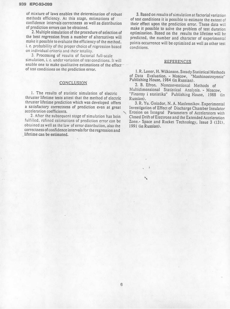
The type of regression function is chosen from a ITT. Estimation of orediction errornumber of models which describe the erosion processmost adequately, based on results of lifetime test Using the statistical simulation method, estimates ofanalytical treatment. The logarithmic model of erosion prediction erroraTp were obtained. Fig. 5 shows 68%

dependence on time takes the form: and 80 % confidence intervals for the relativeY- A In (+ 10 t , ATSAn + prediction error ATp. - - 100% depending on the

where t is time, thousand hours;Y is erosion magnitude (mm), measured over acceleration coefficient K, which constitutes the ratio of

the butt end of the accelerating channel; lifetime T to test time t: K - T/t. The variation rangeA and a are regression coefficients. of T in simulation was 2...6 thousand hours 1000

The coefficients of true regression are chosen to be si m ula t i on s for each I value were performed.close to those obtained in lifetime tests so that thelifetime therewith follows that specified in the Confidence Boundariessimulation, for Prediction Error

As lifetime depends on the critical value of erosion to Ar....% . -a great extent, the program allows for specifying its I 2various magnitudes. -

2. The test duration land the numberof experimental /points n are specified, i.e. pairs of values (i, Yi),i- I,...,n, where YI is the measured value of erosion. ..--

Three versions oft location are stipulated, i. e. the first /being uniform along the time axis, the second 4 - % bouncorresponding to equal increments along the Y axis, the / 1-68 % boundarythird corresponding to equal segments of arc along the % bondaryregression curve.

3. Results of tests Y are simulated with the following 7 9 // 3formula: -

Yi - Y(ti) + ci ,

where Yli) is the value of true regression in the point -ti;

ei - o ul is the error of results of observations; Fig. 5u I is a random magnitude which is distri-

buted according to the normal law -N(O.l);o is the mean-root-square deviation. It is 's

specified to be close to values of residual mean-root- The coefficients of true regression and a weresquare errors that are obtained in the processing of chosen close to their values that were obtained in lifetimeavailable lifetime test results. tests.

4. The simulated test results are treated according to The obtained preliminary results indicate that thethe procedure mentioned above in Section 1. It means prediction error value is reasonable even at sufficientlythat the regression coefficients and the predicted lifetime great values of the acceleration coefficient K.value are derived by the simplex method, possibly using The work on statistic simulation of lifetime tests withrobust procedures, as the value Tp in the regression the aim of evaluating correctness of the method andequation at Y (Tp) - Ycr, where Ycr is the critical value efficiency of the criteria are being continued in theof erosion. following directions:

Among other things, for the logarithmic function the 1. Multiple simulation under various test conditionspredicted value of lifetime is found from the formula: (duration, error of the outcome of observations, the

1 ./ ( Yer number and character of the experimental pointsTP- (ep A - 1) . occurence) at different laws of erosion distribution. The

following laws are meant: normal, lognormal, Weibull5. The prediction error in the simulated test and gamma laws, also mixtures of the normal andA Tp - Tp - T , Cauchy laws and of two normal laws, one of them havingTt is derived in the same manner as T p, but with a great mean-root-square deviation. It is done for the

values of the coefficients A and a corresponding to the purpose of evaluating the effect of deviation from thetrue regression, conventional assumption of the normality of observation

results on the prediction error. In this case the simulation

5

939 IEPC-93-099

of mixture of laws enables the determination of robust 3. Based on results of simulation at factorial variationmethods efficiency. At this stage, estimations of of test conditions it is possible to estimate the extent ofconfidence intervals correctness as well as distribution their effect upon the prediction error. These data willof prediction errors can be obtained, make it possible to solve the problem of test duration

2. Multiple simulation of the procedure of selection of optimization. Based on the results the lifetime will bethe best regression from a number of alternatives will predicted, the number and character of experimentalmake it possible to evaluate the efficiency of the method, points occurrence will be optimized as well as other testi. e. probability of the proper choice of regression based conditions.on individual criteria and their totality.

3. Processing of results of factorial full-scalesimulation, i. e. under variation of test conditions. It will REFERENCESenable one to make qualitative estimations of the effect-of test conditions on the prediction error. 1.R. Loner, H. Wilkinson. Steady Statistical Methods

of Data Evaluation. - Moscow, "Mashinostroyenie"Publishing House, 1984 (in Russian).

ONCLUSN 2. B. Efron. Nonconventional Methods ofMultidimensional Statistical Analysis. - Moscow,

1. The results of statistic simulation of electric "Finansy i statistika" Publishing House, 1988 (inthruster lifetime tests attest that the method of electric Russian).thruster lifetime prediction which was developed offers 3. R. Yu. Gnizdor, N. A. Maslennikov. Experimentala satisfactory correctness of prediction even at great Investigation of Effect of Discharge Chamber Insulatoracceleration coefficients. \ Erosion on Integral Parameters of Accelerators with

2. After the subsequent stage of simulation has bcin Closed Drift of Electrons and the Extended Accelerationfulfilled, refined estimations of prediction error can be Zone.- Space and Rocket Technology, Issue 3 (131),obtained as well as the law of error distribution, also the 1991 (in Russian).correctness of confidence intervals for the regression andlifetime can be estimated.

6