power sharing in dc microgrids
TRANSCRIPT

Rijksuniversiteit Groningen
Faculty of Science and Engineering
Discrete Technology & Production Automation
Power Sharing in DC Microgrids
Master thesis
Author:V.J. (Vincent) Otten
Supervisors:prof. dr. ir. J.M.A.
Scherpen
prof. dr. C. De Persis
M. Cucuzzella, PhD
May 25, 2020

ii

Abstract
A microgrid is an example of a distributed power system. Microgrids are defined as low-voltagedistribution networks which comprise of various small-scale distributed generation units (DGUs),energy storage devices, and controllable loads that are connected through power lines. A microgridmust be controlled in such a way that it presents reliability and proper operation. One of the mainchallenges to assure reliability and proper operation of microgrids is the complex controllabilityof such a system.
In this research, a distributed control scheme is proposed that achieves fair power sharing andweighted average voltage regulation in dynamical DC microgrids. A microgrid is considered whereDGUs are connected through dynamic resistive-inductive power lines and supply so-called ZIP-loads. Furthermore, every distributed generation unit is complemented with a local controller thatcommunicates with neighboring controllers over a communication network. Achieving fair powersharing and weighted average voltage regulation reduces maintenance cost and prevents DGUs forbreakdown which increases the stability and reliability of a power system.The performance of the proposed distributed control scheme is investigated via extensive simula-tions. Many critical scenarios are simulated, including various network topologies, failure of powerand communication lines and plug-and-play of DGUs. The simulation results show promising per-formance of the control scheme. Fair power sharing and average voltage regulation are achievedin most of the scenarios. Besides, the results lead to interesting insights regarding the design ofmicrogrids. Theoretical validation of the control scheme is not included in this thesis and left forfurther research.
iii

iv

Contents
Abstract ii
Contents v
List of Figures vii
List of Tables ix
List of Acronyms ix
List of Symbols xi
1 Introduction 31.1 Research problem and goal . . . . . . . . . . . . . . . . . . . . . . . . . . . . . . . 41.2 Research questions . . . . . . . . . . . . . . . . . . . . . . . . . . . . . . . . . . . . 51.3 Thesis outline . . . . . . . . . . . . . . . . . . . . . . . . . . . . . . . . . . . . . . . 5
2 Theoretical background 72.1 Power systems . . . . . . . . . . . . . . . . . . . . . . . . . . . . . . . . . . . . . . 72.2 Microgrid system . . . . . . . . . . . . . . . . . . . . . . . . . . . . . . . . . . . . . 82.3 DC Microgrid control strategies . . . . . . . . . . . . . . . . . . . . . . . . . . . . . 10
3 Preliminaries 153.1 Notation . . . . . . . . . . . . . . . . . . . . . . . . . . . . . . . . . . . . . . . . . . 153.2 Electrical networks as graphs . . . . . . . . . . . . . . . . . . . . . . . . . . . . . . 15
4 DC Microgrid model 17
5 Distributed control scheme 215.1 Control objectives . . . . . . . . . . . . . . . . . . . . . . . . . . . . . . . . . . . . 22
5.1.1 Power sharing . . . . . . . . . . . . . . . . . . . . . . . . . . . . . . . . . . . 225.1.2 Average voltage regulation . . . . . . . . . . . . . . . . . . . . . . . . . . . . 22
5.2 Control approach . . . . . . . . . . . . . . . . . . . . . . . . . . . . . . . . . . . . . 235.3 Distributed control scheme . . . . . . . . . . . . . . . . . . . . . . . . . . . . . . . 23
5.3.1 Steady state . . . . . . . . . . . . . . . . . . . . . . . . . . . . . . . . . . . . 25
6 Simulations 276.1 Benchmark network . . . . . . . . . . . . . . . . . . . . . . . . . . . . . . . . . . . 28
6.1.1 Power sharing . . . . . . . . . . . . . . . . . . . . . . . . . . . . . . . . . . . 306.1.2 Average voltage regulation . . . . . . . . . . . . . . . . . . . . . . . . . . . . 32
6.2 Power line failure . . . . . . . . . . . . . . . . . . . . . . . . . . . . . . . . . . . . . 346.2.1 Failure of power line k41 . . . . . . . . . . . . . . . . . . . . . . . . . . . . . 366.2.2 Failure of power line k12 . . . . . . . . . . . . . . . . . . . . . . . . . . . . . 40
v

CONTENTS vi
6.2.3 Failure of power line k41 and k12 − isolation of node 1 . . . . . . . . . . . . 446.3 Communication link failure . . . . . . . . . . . . . . . . . . . . . . . . . . . . . . . 486.4 Plug-and-play . . . . . . . . . . . . . . . . . . . . . . . . . . . . . . . . . . . . . . . 52
6.4.1 Plug in DGU 5 . . . . . . . . . . . . . . . . . . . . . . . . . . . . . . . . . . 536.4.2 Plug out DGU 4 . . . . . . . . . . . . . . . . . . . . . . . . . . . . . . . . . 56
6.5 Interpretation of results . . . . . . . . . . . . . . . . . . . . . . . . . . . . . . . . . 59
7 Conclusion 61
8 Limitations and further research 63
Bibliography 65
Appendices 68
A Benchmark network 69A.1 Benchmark LV microgrid network . . . . . . . . . . . . . . . . . . . . . . . . . . . . 69A.2 Reduced benchmark LV microgrid network . . . . . . . . . . . . . . . . . . . . . . 70

List of Figures
2.1 Physical layer of the AC power system (Conejo and Baringo, 2018) . . . . . . . . . 82.2 Typical microgrid architecture (Perez and Damm, 2019) . . . . . . . . . . . . . . . 92.3 Schematic diagram of a generic microgrid with multiple DGUs . . . . . . . . . . . 102.4 Hierarchical control layers of a microgrid (Olivares et al., 2014) . . . . . . . . . . . 112.5 Hierarchical control architecture (Fei et al., 2019) . . . . . . . . . . . . . . . . . . . 122.6 Three DC microgrid control methods (Saleh et al., 2018) . . . . . . . . . . . . . . . 12
4.1 Schematic representation of DGU i and power line k . . . . . . . . . . . . . . . . . 174.2 Schematic representation of the nonlinear load model that is considered in the DGUs 19
5.1 System model with feedback loop controller . . . . . . . . . . . . . . . . . . . . . . 23
6.1 Schematic representation of the benchmark microgrid . . . . . . . . . . . . . . . . 286.2 Power at node i = 1, . . . , 6 . . . . . . . . . . . . . . . . . . . . . . . . . . . . . . . . 306.3 Fair power sharing among DGUs in benchmark network . . . . . . . . . . . . . . . 316.4 Voltage at DGU i = 1, . . . , 6 . . . . . . . . . . . . . . . . . . . . . . . . . . . . . . . 326.5 Average voltage regulation . . . . . . . . . . . . . . . . . . . . . . . . . . . . . . . . 336.6 A schematic representation of a four DGU microgrid network that is considered for
the simulation of the next series of scenarios . . . . . . . . . . . . . . . . . . . . . . 346.7 Failure of power line k41 . . . . . . . . . . . . . . . . . . . . . . . . . . . . . . . . . 366.8 Current flow across edges during failure of power line k41 . . . . . . . . . . . . . . 376.9 Fair power sharing among nodes during failure of power line k41 . . . . . . . . . . 386.10 Weighted average voltage of all the nodes in the network during failure of power
line k41 . . . . . . . . . . . . . . . . . . . . . . . . . . . . . . . . . . . . . . . . . . 396.11 Failure of power line k12 . . . . . . . . . . . . . . . . . . . . . . . . . . . . . . . . . 406.12 Current flow across edges during failure of power line k12 . . . . . . . . . . . . . . 416.13 Fair power sharing among nodes during failure of power line k12 . . . . . . . . . . 426.14 Weighted average voltage of all the nodes in the network during failure of power
line k12 . . . . . . . . . . . . . . . . . . . . . . . . . . . . . . . . . . . . . . . . . . 436.15 Failure of power line k41 and k12, which results in isolation of DGU 1 . . . . . . . . 446.16 Voltage at PCC of DGU 1, . . . , 4 . . . . . . . . . . . . . . . . . . . . . . . . . . . . 456.17 Fair power sharing among DGUs during isolation of DGU 1 . . . . . . . . . . . . . 466.18 Weighted average voltage of all the nodes in the network . . . . . . . . . . . . . . . 476.19 Failure of communication link γ12 . . . . . . . . . . . . . . . . . . . . . . . . . . . . 486.20 Fair power sharing among all DGUs during failure of communication link γ12 . . . 496.21 Measured current (It) at the converter of DGU i = 1, . . . , 4 in the network during
failure of communication link γ12 . . . . . . . . . . . . . . . . . . . . . . . . . . . . 506.22 Weighted average voltage of all the nodes in the network during failure of commu-
nication line γ12 . . . . . . . . . . . . . . . . . . . . . . . . . . . . . . . . . . . . . . 516.23 Plug in DGU 5 . . . . . . . . . . . . . . . . . . . . . . . . . . . . . . . . . . . . . . 536.24 Fair power sharing among all DGUs during plug in of DGU 5 . . . . . . . . . . . . 546.25 Weighted average voltage of connected nodes in the network . . . . . . . . . . . . . 55
vii

LIST OF FIGURES viii
6.26 Plug out DGU 4 . . . . . . . . . . . . . . . . . . . . . . . . . . . . . . . . . . . . . 566.27 Fair power sharing among all DGUs during plug in of DGU 5 . . . . . . . . . . . . 576.28 Weighted average voltage of connected nodes in the network . . . . . . . . . . . . . 58
A.1 Benchmark LV microgrid network (Papathanassiou et al., 2005) . . . . . . . . . . . 69A.2 Reduced benchmark LV microgrid network (Wang et al., 2017) . . . . . . . . . . . 70

List of Tables
3.1 Calligraphic letters and their matrices . . . . . . . . . . . . . . . . . . . . . . . . . 15
4.1 Description of the used symbols . . . . . . . . . . . . . . . . . . . . . . . . . . . . . 18
6.1 Parameter values that remain unchanged during simulations . . . . . . . . . . . . . 276.2 DGU parameters of the benchmark network . . . . . . . . . . . . . . . . . . . . . . 296.3 Line parameters of the benchmark network . . . . . . . . . . . . . . . . . . . . . . 296.4 DGU parameters of the four node network . . . . . . . . . . . . . . . . . . . . . . . 346.5 Line parameters of the four node network . . . . . . . . . . . . . . . . . . . . . . . 346.6 DGU parameters during failure of power line k41 . . . . . . . . . . . . . . . . . . . 366.7 Line parameters after failure of power line k41 . . . . . . . . . . . . . . . . . . . . . 366.8 DGU parameters during failure of power line k41 . . . . . . . . . . . . . . . . . . . 406.9 Line parameters after failure of power line k12 . . . . . . . . . . . . . . . . . . . . 406.10 DGU parameters during failure of power line k41 and k12 . . . . . . . . . . . . . . 446.11 Line parameters after failure of power line k41 and k12 . . . . . . . . . . . . . . . . 446.12 DGU parameters when DGU 5 is plugged in. . . . . . . . . . . . . . . . . . . . . . 536.13 Line parameters after DGU 5 is plugged in . . . . . . . . . . . . . . . . . . . . . . 536.14 DGU parameters after DGU 4 is plugged out . . . . . . . . . . . . . . . . . . . . . 566.15 Line parameters after DGU 4 is plugged out . . . . . . . . . . . . . . . . . . . . . . 56
ix

LIST OF TABLES x

List of Acronyms
AC Alternating Current
DC Direct Current
DERs Distributed Energy Resources
DGUs Distributed generation units
GCOP Grid connected operating mode
IOM Islanded operating mode
LQR Linear quadratic regulator
MG Microgrid
MGCC Main grid central controller
PCC Point of common coupling
PID Proportional integral derivative
PnP Plug-and-play
PV Photovoltaic
RES Renewable energy source
SPOF Single point of failure
xi

LIST OF TABLES xii

List of Symbols
Calligraphic letters
A Adjacency matrix
B Incidence matrix
D Degree matrix
E Set of edges
Ecom Set of communication edges
L Laplacian matrix
Lcom Laplacian matrix of the communication network
Ni Set of nodes neighbouring node i
V Set of nodes
Alphabet
Cti Capacitance of DGU i
I∗k Current at power line k
Ili Load demand at DGU i
I∗li Constant current load at DGU i
I∗ti Generated current at DGU i
Ki Tuning parameter of DGU i
kij Power line connecting DGU i and j
Lk Inductance at line k
Lti Inductance at DGU i
m Number of power lines in the network
mc Number of communication links in the network
n Number of distributed generation units (DGUs) in the network
Pi Power at source node i
P ∗ Power convergence value
P ∗li Constant power load at DGU i
Rk Resistance at power line k
xiii

LIST OF TABLES 1
Tθi Tuning parameter of DGU i
Tφi Tuning parameter of DGU i
ui Control input
V Vector of voltages
Vi Voltage at PCC of DGU i
V ∗ Reference voltage
W Matrix of weights assigned to DGUs
wi Weight assigned to DGU i
Z∗li Constant impedance load at DGU i
Greek alphabet
Γ Matrix of communication link weights
γij Weighted communication link connecting node i and node j
θ Controller’s state variable
φ Controller’s state variable

LIST OF TABLES 2
Chapter 1
Introduction
Economical, technological and environmental incentives are changing the face of electricity gen-eration and transmission (Lasseter and Piagi, 2004). In the past years, many countries havebegun the transition of their energy systems towards a more sustainable energy supply based onrenewable energies. A trend is recognised that countries transforming their energy systems froma rather centralised approach with continuous energy generation based on fossil fuels to a moredecentralised system with fluctuating energy generation from thousands of energy production fa-cilities (e.g. wind, solar, and biomass) (DENA, 2019).Centralized generation refers to the large-scale generation of electricity at centralized facilities.These facilities are usually located away from end-users and connected through a network ofhigh-voltage transmission lines. The electricity generated by centralized generation is distributedthrough the electric power grid to multiple end-users. Centralized generation facilities includefossil-fuel-fired power plants, nuclear power plants, hydroelectric dams, wind farms, and more(EPA, 2018a).On the contrary, a variety of small-scale technologies that generate electricity at or near where itwill be used is referred as distributed generation (EPA, 2018b). Distributed generation of elec-tricity offers numerous benefits in comparison to the conventional centralized systems. Importantbenefits of decentralized power generation systems are no high peak load shortages, reduced hightransmission and distribution losses, linking remote and inaccessible areas, faster response to newpower demands, and improved supply reliability and power management (ISGF, 2019).
Recent trends of increasing electricity demands for critical infrastructure have led to increasinginterest in microgrids. Microgrids are defined as low-voltage distribution networks which compriseof various small-scale distributed generator units (DGUs), energy storage devices, and controllableloads that are connected through power lines. The small-scale generation units usually have aproduction capacity of 10 megawatts or less.In contrary to traditional centralised power system, microgrids can can operate either in grid-connected mode, or in islanded mode. In grid connected mode, the microgrid decit power mustbe supplied by the main grid, and the excess power produced in the microgrid must be sent tothe main grid (de Souza and Castilla, 2019). If the main grid supplies power to microgrid, themain power-grid acts as an controllable voltage source (Venkatraman and Khaitan, 2015). Inisland mode, the microgrid operates independently from the main grid (Arif and Hasan, 2018), forexample in aircrafts and ships. These microgrids have many advantages over traditional energydistribution systems, like the increase in reliability, power quality improvement, and a reductionin distribution network losses (Rahmani et al., 2017).
Nowadays there exist several examples of small DC microgrids, as in marine, aviation, automotive,and manufacturing industries. In all these examples it is extremely important that the microgridis controlled such a way that it presents reliability and proper operation. Microgrids should be
3

1.1. RESEARCH PROBLEM AND GOAL 4
able to locally solve energy problems and hence increase flexibility (Guerrero et al., 2012a).One of the main challenge to assure reliability, flexibility and proper operation of microgrids isthe complex controllability of such a system (Rahmani et al., 2017). In a microgrid with multipledistributed generation sources, fair power sharing is an important aspect for the reliability of DGUin a microgrid. Fair power sharing means that the total demand of the microgrid is shared amongall DGUs proportionally to the generation capacity of their corresponding energy sources. Thiscontrol method prevents local generation units from exceeding their maximum generating capacity,to reduce maintenance cost and prevent for breakdown of DGUs which results in instability andunreliability of the power supply system. Besides, the autonomous operation of a microgridrequires local control strategies to maintain voltage at acceptable levels (Trip et al., 2014). Due tothe increased interest in DC microgrids, the literature on DC microgrids from a control-theoreticperspective is rapidly growing. Many current, voltage and power sharing techniques, approachedby different control strategies, are proposed literature.
1.1 Research problem and goalAs outlined in the previous section, reliability and the stability of the power power supply in amicrogrid is important for numerous reasons. Especially when the microgrid operates in islandedmode, it is fully dependent of the power sources in the network. In order to increase the reliabilityand stability of a power system, power sources should be prevented for exceeding its generationlimit, which can cause damage to distributed generation units and cause instability and unrelia-bility of the power system. Therefore, DGUs in a microgrid should be controlled in such a waythat the sources are prevented for exceeding their generation limit. Secondly, voltage regulationin DC microgrid is included, so that the voltages in the microgrid is maintained within acceptablelimits.
This research aims to design a distributed control scheme that achieves fair power sharing andweighted average voltage regulation in dynamical DC microgrids. The power that is generatedby every distributed generation unit (DGU) in a microgrid is proportional to the generationcapacity of the corresponding DGU. In the microgrid considered in this thesis, multiple DGUs areinterconnected through dynamic resistive-inductive (RL) power lines and supply so-called ZIP-loads i.e., nonlinear loads with the parallel combination of unknown constant impedance (Z),current (I) and power (P) components.After a distributed control scheme that achieves fair power sharing is proposed, the performance ofthe control scheme analysed via extensive simulations in MATLAB. Critical and realistic scenariosare considered for simulations that include: various network topologies, plug-and-play scenariosand possible failure of power lines and communication scenarios.After the proposed control scheme is analysed, interesting new insights regarding the design of amicrogrid are provided, to improve the stability and reliability of such a system.
Therefore, the main objectives of this research are summarized in the following research goal:
Design a distributed control scheme that achieves fair power sharingand weighted average voltage regulation in DC microgrids, and analyse
the performance of the proposed control scheme
1.2. RESEARCH QUESTIONS 5
1.2 Research questions
In order to reach the research goal in a structural manner, the following research questions (RQs)are posed:
RQ 1: What are the available control strategies to control DC microgrids?This knowledge question provides prior knowledge of control strategies of DC microgrid,which is essential to design the control scheme
RQ 2: What are the mathematical tools required to develop the models in this thesis?This knowledge question provides preliminaries required for the subsequent questions
RQ 3: How will a DC microgrid be modeled?This design question provides the differential equations that describe the behaviour of thedynamical DC microgrid
RQ 4: How will the control scheme be modeled?This design question provides the differential equations that describe the dynamical behaviourof the proposed distributed control scheme. Together with the differential equations of the DCmicrogrid, the dynamical behaviour of the overall system is described
RQ 5: What realistic and critical scenarios will be used to analyse performance of theproposed control scheme?This design question provides under which realistic circumstances the control scheme is tested
RQ 6: How does the control scheme, that is proposed in this thesis, performs in criticalcircumstances?This question provides an analysis of the performance of the control scheme
RQ 7: To what new insights lead the analysis of the proposed control scheme?This question provides new insights with regard to the design of microgrids
RQ 8: What conclusions can be drawn from the analysis of the proposed distributed controlscheme?This knowledge question determines the main conclusions of the thesis, in order to addknowledge to existing literature, while also discussing current limitations and potential areasfor further work
Answering the research questions mentioned above will result in achieving the research goal thatis stated in section 1.1.
1.3 Thesis outlineThe research questions posed above are generally answered in numerical order throughout thethesis. The remainder of this thesis is outlined as follows:
Subsequent to the introduction, chapter 2 covers the theoretical background of the thesis whichforms the backbone of this work. The chapter discusses the current trends in power systemswhich supports the relevance of DC microgrids. Furthermore, current available control strategiesof DC microgrids are discussed to provide understanding of control operations in DC microgrid.A control strategy from the available control strategy is chosen and justified which leads the restof the thesis.
Secondly, in chapter 3 discusses the preliminaries for the remainder of the thesis. This chapterprovides the tools that are used in models that are developed in the subsequent chapters, butcould be skipped by the experienced reader. This chapter answers research question 2.

1.3. THESIS OUTLINE 6
In chapter 4, a DC microgrid model is developed, using the tools that are discussed in chapter 3.This DC microgrid model is used to develop a control scheme for, which is predestined in the nextchapter. This chapter answers research question 4.
In chapter 5, a distributed control scheme is designed that achieves fair power sharing among thedistributed generation units (DGUs) the DC microgrid model that is developed in chapter 4. Thischapter answers research question 5.
Subsequently, chapter 6 follows from chapters 4 and 5. In this chapter, the performance if theproposed distributed control scheme (designed in chapter 5) for the DC microgrid model (developedin chapter 4) is investigated through simulation of critical and realistic scenarios using MATLAB.These scenarios include variation of network topology, plug-n-play scenarios, failure of power linesand failure of communication between DGUs. Besides, from the simulation results, interestingnew insights are determined. This chapter answers research question 5, 6 and 7.
Finally, research question 8 is addressed in chapter 7, in which concluding remarks are providedand the thesis is concluded by discussing limitations of the current research project and highlightingpotential areas for further work in chapter 8
Chapter 2
Theoretical background
This chapter provides a theoretical background on power networks, microgrids and the control ofmicrogrids. The goal of this section is to provide a theoretical framework of the principles that areused in the rest of this work. Research question 2 is answered in this chapter. In section 2.1 andsection 2.2 theory and trends of power systems and microgrid systems is provided to emphasisethe relevance of control of DC microgrids, not only now but but also in the future. In section 2.3,different control strategies that are currently available in literature are highlighted and the sectionelaborates on a control approach where the rest of thesis continuous on. Research question 1 isanswered in this chapter.
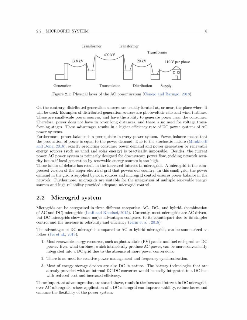
2.1 Power systemsThe power network can be regarded as one of the most important infrastructures the world knows(Trip et al., 2020). The demand for electrical energy in the 21st century is increasing worldwideand a fast development in the area of renewable energy sources is required to overcome the en-vironmental issues related to the reduction of greenhouse gases (Rinaldi et al., 2017). Since thevery beginning, it has been an issue of debate regarding the choice of alternating current (AC) ordirect current (DC) as system of electrical power transfer (Datta et al., 2018).According to the history perspectives, AC power network has been the standard choice for commer-cial energy systems (Justo et al., 2013). Traditionally, large-scale power generation at centralizedfacilities are usually located away from end-users (EPA, 2018b). Therefore, AC distribution isused intensively due to long distances power has to cover, because alternating current have abil-ity to easily change the voltage level throughout the system (Datta et al., 2018). To distributethe power from generation over multiple consumers, the power is transformed to various (high)voltages levels, as shown in Figure 2.1 (Conejo and Baringo, 2018).
The primary reason to transform power to high voltage, is to increase transmission efficiency.However, voltage transforming stages in AC power system are inefficient and results in powerlosses (Setiawan et al., 2016b).
7
2.2. MICROGRID SYSTEM 8
Figure 2.1: Physical layer of the AC power system (Conejo and Baringo, 2018)
On the contrary, distributed generation sources are usually located at, or near, the place where itwill be used. Examples of distributed generation sources are photovoltaic cells and wind turbines.These are small-scale power sources, and have the ability to generate power near the consumer.Therefore, power does not have to cover long distances, and there is no need for voltage trans-forming stages. These advantages results in a higher efficiency rate of DC power systems of ACpower systems.Furthermore, power balance is a prerequisite in every power system. Power balance means thatthe production of power is equal to the power demand. Due to the stochastic nature (Mirakhorliand Dong, 2016), exactly predicting consumer power demand and power generation by renewableenergy sources (such as wind and solar energy) is practically impossible. Besides, the currentpower AC power system is primarily designed for downstream power flow, yielding network secu-rity issues if local generation by renewable energy sources is too high.These issues of debate has result in the increased interest in microgrids. A microgrid is the com-pressed version of the larger electrical grid that powers our country. In this small grid, the powerdemand in the grid is supplied by local sources and microgrid control ensures power balance in thenetwork. Furthermore, microgrids are suitable for the integration of multiple renewable energysources and high reliability provided adequate microgrid control.
2.2 Microgrid systemMicrogrids can be categorised in three different categories: AC-, DC-, and hybrid- (combinationof AC and DC) microgrids (Lotfi and Khodaei, 2015). Currently, most microgrids are AC driven,but DC microgrids show some major advantages compared to its counterpart due to its simplercontrol and the increase in reliability and efficiency (Jerin et al., 2018).
The advantages of DC microgrids compared to AC or hybrid microgrids, can be summarized asfollow (Fei et al., 2019):
1. Most renewable energy resources, such as photovoltaic (PV) panels and fuel cells produce DCpower. Even wind turbines, which intrinsically produce AC power, can be more convenientlyintegrated into a DC grid due to the absence of more power conversions.
2. There is no need for reactive power management and frequency synchronization.
3. Most of energy storage devices are also DC in nature. The battery technologies that arealready provided with an internal DC-DC converter would be easily integrated to a DC buswith reduced cost and increased efficiency.
These important advantages that are stated above, result in the increased interest in DC microgridsover AC microgrids, where application of a DC microgrid can improve stability, reduce losses andenhance the flexibility of the power system.

2.2. MICROGRID SYSTEM 9
As mentioned in the introduction, a microgrid refers to a set of distributed generation units(DGUs), control systems and loads that can independently supply the power required for theconsumers with high reliability. (Beykverdi et al., 2017). Figure 2.2 shows a typical microgridarchitecture that consist of power sources, storage capacity and loads.
Figure 2.2: Typical microgrid architecture (Perez and Damm, 2019)
Power sources that are used in microgrids, such as photovoltaic panels, fuel cells, and batterybanks operate in DC mode and are located near the loads. In addition, various loads such ascomputers, TVs, and LED bulbs are supplied with direct current (de Souza and Castilla, 2019),which eliminates power losses at conversion stages in a microgrid, since the supply and load areboth in DC mode. However, not every power generator produces DC power, since most turbines(wind, hydro, or steam) produce AC power.
Renewable energy resources such as wind and solar are an important component of a micro-grid. However, the inherent intermittency and variability of such resources complicates microgridoperations. Meanwhile, more loads, distributed generators (e.g., micro gas turbines and dieselgenerators), and distributed energy storage devices (e.g., battery banks) are being integrated intothe microgrid operation (Su et al., 2013). Normally, the distributed energy storage system in a mi-crogrid will only supply power when the total load demand exceeds the power generation capacityof DGUs in a microgrid (Beykverdi et al., 2017). In this thesis, the all power sources e.g. renewableenergy sources, distributed generators and distributed energy storage systems are assumed to becontrollable distributed generation units (DGUs), which implies that the intermittance of naturedoes not affect the power supply.
In general, a microgrid can have a schematic configuration as shown in Figure 2.3, where mulitpleDGUs are connected to various loads through microgrid network. The microgrid is connected tothe main grid at the point of common coupling (PCC). A microgrid is able to operate in gridconnected operation mode (GCOM), or in islanded mode (IOM) i.e. when the microgrid is notconnected to the main grid (Cucuzzella et al., 2018a). Several control techniques are reported inthe literature to control microgrids either in GCOM or IOM (Incremona et al., 2016).In grid-connected mode, the main grid can provide ancillary services to balance the supply anddemand of power if the supplied power does not meet the load demand. When the microgrid is in

2.3. DC MICROGRID CONTROL STRATEGIES 10
grid-connected mode. When the microgrid operates in island mode, the power that is generatedwithin the microgrid, including the temporary power transfer from/to storage units, should bebalanced with the total demand of the loads in the network. A DC microgrid in islanded operatingmode is particularly interesting since IOS offer several promising advantages in reducing powerlosses, smoothly integrating RES and increasing the network resiliency (Cucuzzella et al., 2017).Besides, microgrids should preferably tie to the utility grid so that any surplus energy generatedwithin the microgrid can be channeled to the utility grid (Guerrero et al., 2012b).
Figure 2.3: Schematic diagram of a generic microgrid with multiple DGUs
2.3 DC Microgrid control strategiesAdvanced control strategies are vital components for realization of microgrids. It is extremelyimportant that the microgrid is controlled such a way to present reliability and proper operation.To attain this goal, there are many control strategies. The most popular control technique isa linear control. It has gain its popularity due its simplicity and robustness. However as thename suggest, linear control considers a model that is linearized around an operating point. Thisimplies that the simplified model is only valid around the operating point. Several approaches areavailable for linear control in microgrids. Examples are: transfer functions or state space modeling,where proportional integral derivative (PID), state feedback and linear–quadratic regulator (LQR)allocation of poles are viable strategies (Perez and Damm, 2019).On the other hand, nonlinear control technique is based on the complete model of the system.This means the the nonlinear operation dynamics are included. The advantage of nonlinear controlstrategy is the more realistic grid modeling and that the model is not restricted to operate aroundthe operating point. However a drawback of nonlinear control strategy is the increased complexityof analysis and the challenging implementation of the control law.
To ensure proper control of the microgrid, hierarchical control in different layers is implemented.These control layers provide certain degree of independence between different control levels. Be-sides, multiple control layers have the advantage to be more reliable as it continues to be oper-ational even in the case of failure of the centralized control layer. (Fei et al., 2019). Figure 2.4shows the three layers that are used in hierarchical microgrid control.

2.3. DC MICROGRID CONTROL STRATEGIES 11
Figure 2.4: Hierarchical control layers of a microgrid (Olivares et al., 2014)
Conventionally, hierarchical control schemes are proposed to achieve current, voltage and powersharing (Fei et al., 2019). Figure 2.5 shows the hierarchical control architecture including primary,secondary and tertiary control level. The bandwidth, is the response time of the system. It is ameasure of the time it requires to responds to a change of the input command. The figure showsthat primary includes the fastest response time versus tertiary control which requires to most timeto response to a change of variables within the system.

2.3. DC MICROGRID CONTROL STRATEGIES 12
Figure 2.5: Hierarchical control architecture (Fei et al., 2019)
Primary control, also known as local control or internal control, is the first layer in the controlhierarchy, including the fastest response. This control layer operates in a time range of a fewseconds (Perez and Damm, 2019). The responsibility of the primary control layer is to regulatethe current en voltage in the microgrid to adapt the grids operating points when disturbanceacts on the system during the period the secondary controller requires to calculate the new set ofoptimal operation values.
Secondary control is responsible for the power quality. this implies the optimal power flowto ensure power balance in the system. This control layer regulates the power that is generatedfor each power source in the network. From a communication based perspective, the secondarycontrol layer can be implemented in three different manners, as shown in Figure 2.6.
Figure 2.6: Three DC microgrid control methods (Saleh et al., 2018)
The different manners to implement the secondary control layer are shortly discussed below: (Salehet al. (2018), Perez and Damm (2019))

2.3. DC MICROGRID CONTROL STRATEGIES 13
In decentralized control, no communication is required. This control technique only usesmeasured local information to define its control actions. Therefore, all the DGUs can operatein parallel and are not depend of each other or of communication.
In centralized control, all sensors’ data (e.g. microgrid states) is are transmitted fromthe DGUs to a central controller (MGCC). This central controller processes all the incomingdata and sends back actions of control. Since the central controller has real-time data of allthe power sources, it can reach or approach optimal performance of the microgrid. However,a drawback is that the controls reliability depends on the reliability of the communicationnetwork.
In distributed control no central controller is required. DGUs communicate their statesonly to their direct neighbours to achieve optimal performance. The main advantage ofthis method is that a DGU is only dependent of the communication between itself and itsneighbours. Therefore, the system can maintain full functionality, even if the failure of somecommunication links occurs, provided that the communication network remains connected.This implies that distributed control is immune to a single point of failure (SPOF).
Finally, tertiary control is the highest layer in the hierarchy control scheme, including the slowestresponse time. This layer deals with the energy market, organizing the energy dispatch scheduleaccording to an economic point of view, taking into account negotiation between consumers andproducers. This level also deals with human–machine interaction and social aspects (Perez andDamm, 2019).
In order to design a control scheme that achieves fair sharing, which is a goal of this thesis, thecontrol law is placed in the secondary layer of the hierarchical control scheme. The proposedcontrol scheme is based on distributed control, since this control method has most potential toachieve high reliability and quality of the power supply in a microgrid due to its immunity forSPOF, local information sharing and low dependency.

2.3. DC MICROGRID CONTROL STRATEGIES 14

Chapter 3
Preliminaries
This chapter provides a theoretical background on power system dynamics, presenting requiredpreliminaries for the subsequent chapters. This chapter contains notation and concepts that areapplied in the remainder of the research and answers research question 3.
3.1 NotationThroughout this thesis, N and R denote the set of natural and real numbers, respectively. Fur-thermore, 1n ∈ Rn×1 denotes a column vector of ones, In denotes an identity matrix of size n,and denotes the Hadamard (entrywise) product.
Secondly, the calligraphic letters used in this research are reserved for the following matrices:
Table 3.1: Calligraphic letters and their matrices
Calligraphic letter MatrixA Adjacency matrix of a graphB Incidence matrix of a graphD Degree matrix of a graphL Laplacian matrix of a graphLcom Laplacian matrix of a communication graph
3.2 Electrical networks as graphsIn network theory, a DC power network is represented by a connected and undirected graphG = (V, E). The graph consist of a set of nodes V = 1, . . . , nv, which represents the DGUs anda set of edges E = 1, . . . , ne, which represent the power lines interconnecting the DGUs.
The network topology is described by its corresponding incidence matrix that consist of V ∈ Rnand E ∈ Rn, which relates nodes to their connected edges. The incidence matrix B ∈ Rn×m. thelabels are arbitrarily labeled with a + and a − where the entries of B are given by
Bi,k =
+1 if node i is connected to the positive end of edge k−1 if node i is connected to the negative end of edge k0 otherwise.
(3.1)
15

3.2. ELECTRICAL NETWORKS AS GRAPHS 16
Similarly, the communication network is represented by a connected and undirected graph Gcom =(V, E). The graph consist of a set of nodes V = 1, . . . , nv, which represents the DGUs and a setof edges E = 1, . . . , ne, which represent the communication lines interconnecting the DGUs.The incidence matrix for the communication network, Bcom ∈ Rn×mc , describes the networktopology nodes that communicate with each other.
Bcomi,k =
+1 if node i is connected to the positive end of communication edge k−1 if node i is connected to the negative end of communication edge k0 otherwise.
(3.2)
In this research, the incidence matrices are used to model the power flow and communicationbetween the nodes.

Chapter 4
DC Microgrid model
In this chapter, a DC microgrid model is developed to answer research question 4. The model isa typical DC microgrid model, which consist of n distributed generation units (DGUs) that areconnected through m resistive-inductive (RL) power lines. Furthermore, mc communication linksconnects DGUs. This does not necessarily mean that there is a communication link between everyDGU, but it does mean that every DGU communicates with at least one other DGU. Therefore,the physical network topology can be different from the communication network topology.
A schematic representation of a DGU and RL-power lines that interconnect DGUs is given below:
Figure 4.1: Schematic representation of DGU i and power line k
17

18
The symbols used in Figure 4.1, Equation 4.1 and Equation 4.3 are described in Table 4.1
Table 4.1: Description of the usedsymbols
State variablesIti Generated currentVi Load voltageIk Line current
ParametersLti Filter inductanceCti Shunt capacitanceRij Line resistanceLij Line inductance
ZIP-loadsZ∗li Constant impedanceI∗li Constant currentP ∗li Constant power
Inputsui Control inputIli Unknown current demand
Buck converterThe first element is typically an energy source of renewabletype, which can be represented by a direct current (DC)voltage source. The DC voltage source supplies voltage toa DC buck converter. A buck converter (step-down con-verter) is a DC-to-DC power converter which steps downvoltage, while stepping up current. Buck converters areusually highly efficient (> 90 %).Due to this buck converter the voltage that is supplied tothe loads can be controlled as an function of the currentfrom the source. Variable ui denotes the control input, inunits of voltage. The dynamics of the buck are neglected.
LC-filterThe current supplies the loads via a LC filter, consisting ofa inductor and a resistor. The inductor is placed in seriesand the conductor is is placed in parallel to the voltagesource. The filter acts as a resonant which stores energy inthe inductor and capacitor to damp oscillations, occurringin the circuit.
PCCThe point of common coupling (PCC) denotes the pointwhere the DGU is connected to the main grid. In normalmode, the microgrid is connected to the utility grid. The utility grid acts as an DGU. Whenthe microgrid operates in island mode, the microgrid is not connected to the main grid and nowpower is supplied via the point of common coupling. In Equation 4.1, the load currents (Ili) arelocated at the PCC of each DGU. This is generally obtained by a Kron reduction of the originalnetwork (Trip et al., 2018). The Kron reduction of networks is ubiquitous in circuit theory andrelated applications in order to obtain lower dimensional electrically-equivalent circuits (Dorflerand Bullo, 2012).
The equations describing the dynamical behaviour of DGU i, as depicted in Figure 4.1, are givenby
LtiIti = −Vi + ui (4.1a)
CtiVi = Iti − Ili −∑k∈Ei
Ik (4.1b)
LoadsIn this research, a general nonlinear load model is considered that consist of three different type ofloads. Loads in a power network can be broadly classified into two groups: nonactive and activeloads. Common examples for nonactive loads are constant impedance (Z∗l ) loads and constantcurrent (I∗l ), while constant power (P ∗l ) is a active load (Cucuzzella et al., 2019a). The loadsare placed in parallel as shown in Figure 4.2. A constant current load is a load that adjusts itsresistant to maintain a constant current. A constant impedance load is a load that presents anunchanging impedance and a constant power load refers to a load that can maintain a constantinput power regardless of the input voltage supplied. Constant power loads have a nonlinearrelationship between input voltage and load current (Leonard, 2014). Due to the advancementin power electronics in the past decade, a considerable percentage of the loads consists of activeloads (e.g. motor drives, power converters and electronic devices), which often behave as constantpower loads (Cucuzzella et al., 2019a).

19
The ZIP-loads model denotes a parallel combination of the following components:
Z | constant impedance: Ili = Z∗−1li Vi, with Z∗li ∈ R>0
I | constant current: Ili = I∗li, with I∗li ∈ R≥0, and
P | constant power: Ili = V −1i P ∗li, with P ∗li ∈ R≥0
Figure 4.2: Schematic representation of the nonlinear load model that is considered in the DGUs
The total load demand (Ili) is the summation of the three loads when the loads are connected inparallel as shown in Figure 4.2. It is assumed that all the loads are not measurable. Accordingly,the presence of nonlinear ZIP-load in the DGU model, Ili in Equation 4.1b is given by:
Ili (Vi) := Z∗−1li Vi + I∗li + V −1
i P ∗li (4.2)
As mentioned in chapter 3, the overall DC microgrid system is modeled as an undirected graphG = (V, E), with its corresponding incidence matrix B ∈ Rn×m to describe the network topology.
Consequently, the overall DC microgrid system can be written compactly as:
LtIt = −V + u
CtV = It + BI − (Z∗l −1V + I∗l + [V ]−1P ∗l )LI = −BV −RI
(4.3)
Where It, V, Il, I∗l , P ∗l , u ∈ Rn and I ∈ Rm. Furthermore, Ct, Lt, Z∗l ∈ Rn×n and R,L ∈ Rm×mare positive definite diagonal matrices, e.g. Ct = diag(Ct1 , . . . Ctn)
Moreover, I, It and V are the steady state solutions to Equation 4.3 that satisfy the system ofdynamics:
V = u (4.4a)It = (Z∗l −1V + I∗l + [V ]−1P ∗l )− BI (4.4b)I = −R−1B>V (4.4c)
At steady state condition, Equation 4.4a shows that the voltage supplied by the voltage sourceis equal to the control input u. Besides, Equation 4.4b shows that the current that generatedcurrent is equal to the current that is demanded by the loads together with the current that isflows through power lines to neighbouring nodes. Thirdly, the total current that flows throughpower lines to neighbouring nodes j, equal to the current leaving node i. Together, all threeequations should hold to satisfy the steady state condition for the dynamics of the DGU model.

20

Chapter 5
Distributed control scheme
In this chapter, a distributed control scheme is designed which aims to achieves fair power shar-ing and average voltage regulation. Research question 5 is answered in this chapter. To recall,fair power sharing means that every distributed generation unit in a DC microgrid generates theamount of power relative to its maximum production capacity and the maximum production ca-pacity of DGUs in the network. Elementary, a power network contains a generator and consumers.To meet the consumers demand, the generator should produce as much power as the consumers useto achieve and maintain power balance in the power system. In reality, there are many consumersand also multiple producers (Weitenberg, 2018). Taken into account the increase popularity ofsolar panels and other renewable energy sources, many agents of the electrical distribution net-work are prosumers, playing an active role by producing and consuming energy (Cucuzzella et al.,2019b). There could be as many producers as consumers in a power network, each with a limitedgeneration capacity. In fact, every power source has a limited capacity. This means that if some-one turns on a machine that demands a lot of power, that load should be shared among the powersources. This motivates the consideration of power sharing, The simplest form of power sharingrequires that each producer injects the same amount of power into the network at steady state.Of course, in reality, different power sources have different capacities. Therefore, we often aim forweighted power sharing instead, which gives each producer a weight, and balances the weightedpower injections (Weitenberg, 2018).
21

5.1. CONTROL OBJECTIVES 22
5.1 Control objectivesAs mentioned, the control scheme that is proposed in this chapter, aims to achieve fair powersharing and weighted average voltage regulation. The two objectives are discussed in this section.
5.1.1 Power sharingThe primary objective of the control scheme is to achieve fair power sharing at steady state.This implies weighted power sharing at steady state, since the weights corresponds to the powergeneration capacity of DGUs in the network, which are preset by the operator. The controlobjective is to guarantee that at steady state the following identities hold:
wiPi = wjPj , ∀i, j ∈ V (5.1)
Where the power at a DGU i converges to its steady state solution for all i ∈ V:
limt→∞
Pi(t) = Pi (5.2)
Where Pi is the the injected power at node i at steady state. According to Ohm’s law, Pi = ViIti. Hence, P is the vector of power injections at the nodes. Therefore, the fair power sharingobjective, can be written as an expression where the steady state power injections converge to aweighted power convergence value P ∗:
P = W−11P ∗, P ∗ ∈ R (5.3)
with W = diag(wi, . . . , wn), w > 0 for all i ∈ V and P ∗ any scalar. To define an expression forP ∗, Equation 5.3 is multiplied with 1>, to arrive at:
1>P = 1>[It]V = 1>W−11P ∗ (5.4)
After rewriting,
P ∗ = 1>[It]V1>W−11 (5.5)
Besides, to obtain an expression for It, the steady state current balance in Equation 4.4b ismultiplied with 1>:
1>Il = 1>It = Z∗l−1V + I∗l + [V ]−1P ∗l (5.6)
Since 1>B = 0. To this end, the power convergence value P ∗ is expressed as:
P ∗ = 1>([Z∗l ]−1[V ] + [I∗l ] + [V ]−1[P ∗l ])V1>W−11 (5.7)
It is observed that the steady-state injections Equation 5.2 achieves power sharing, and the asymp-totic power value P ∗ to which the source power injections converge in a proportional fashion, isthe total power injected divided by the weights. Therefore, when Equation 5.2 holds, the powerat the DGUs converge to the reference power value and fair power sharing is achieved.
5.1.2 Average voltage regulationThe second objective is to achieve weighted average voltage regulation. Weighted average voltageregulation means that the weighted average of all DGUs in the network, converge to a presetreference voltage value (P ∗), given as initial condition. Therefore, the weighted average value ofV should converge to the weighted desired reference voltage value V ∗ at steady state. This resultsin the following objective where again the DGU with the largest capacity is assigned with thehighest weight:

5.2. CONTROL APPROACH 23
limt→∞
1>W−1V (t) = 1>W−1V = 1>W−1V ∗ (5.8)
The reason to include this objective is when power sharing is achieved, it does not necessarily meanthat when fair power sharing is achieved, voltage levels at DGUs maintain within acceptable limits.Factors such as increased loading and distributed generation contribute to the difficulty in main-taining steady state voltages within prescribed limits (O’gorman and Redfern, 2004). Exceedinglocal voltage limits, can cause stability issues.
5.2 Control approachIn this section, a control scheme is designed that aims to achieve two objectives simultaneously.The primary objective is to achieve fair power sharing among all the DGUs in the network, asdescribed in chapter 1. Besides, the second objective is weighted average voltage regulation of allthe DGUs in the network.In order to achieve weighted power sharing and average voltage regulation, the system is modeledwith a feedback loop controller. As discussed in chapter 4, the system dynamics are described bythree time dependent state variables, namely: voltage at PCC (Vi(t)), generated current (Iti(t))and exchange current (Ii(t)) for all i ∈ V
Figure 5.1: System model with feedback loop controller
As mentioned in chapter 4, the dynamics of the DC microgrid are described by three state vari-ables, which are dependent of the system initial conditions and system parameters. As mentioned,the operator of the DC microgrid preset a reference voltage value where the weighted averagevoltage should converge to.In order to achieve fair power sharing and weighted average voltage regulation, the control schemeis designed with two additional state variables, θ and φ, which can be tuned by controller param-eters parameters (Tφ, Tθ). With use of the buck converter, the control input u is able to adjustthe generated current as a function of voltage. Control input u is complemented with an tuningparameter K.
5.3 Distributed control schemeHowever microgrid model that is considered in this research is fairly standard, the control schemehave some unique features compared to control schemes that are proposed in literature thatachieves power, current, and voltage regulation (Weitenberg (2018), Cucuzzella et al. (2018b),

5.3. DISTRIBUTED CONTROL SCHEME 24
Tucci et al. (2018)). These unique featurs increase the applicability of the control scheme tocontrol microgrids. The following features characterize the uniqueness of the proposed controlscheme:
• resistive and inductive power lines are included, which increase the complexity of the systemdynamics
• nonlinear ZIP-loads are included
• it is not needed to know the ZIP-load demands (Z∗li, I∗li and P ∗li). Only measurement ofpower (Pi) is required (i.e. measurement of voltage at PCC (Vi) and generated current (Iti))
• the control scheme is independent of the initial conditions
• the topology of the communication network can be designed independently of the topologyof the microgrid notwork
• the control scheme is independent of the microgrid parameters
The controller that is designed in this section is inspired by Trip et al. (2018), who propose adistributed control scheme that achieves current sharing and average voltage regulation. For thedesign of the control scheme, two assumptions are made. The first assumption is that the generatedcurrent (Ili) is measurable at the converter, and the voltage is measurable at the PCC of everyDGU in the network. Secondly, it is assumed that there exist a reference voltage (V ∗) for everyDGU in the network that is preset by the operator.
The control scheme is proposed in the following manner:
θi = −∑j∈N c
i
γij (wiItiVi − wjItiVi) (5.9a)
φi = −φi + Iti (5.9b)
ui = −Ki (Iti − φi) + wi∑
j∈N comi
γij (θi − θj) + V ?i (5.9c)
Where N ci denotes the set of DGUs which communicate with the ith DGU. γij = γji ∈ R>0
are the weights of the communication links. wi, wj ∈ R>0 are the weights depending on thegeneration capacity of the DGU. Following the standard practise where the sources with thelargest generation capacity determine the grid voltage, we select a weight of 1
wifor all i ∈ V. Let
Lcom denote the weighted Laplacian matrix of the communication network, which can be differentfrom the Laplacian matrix of the physical network.
From Equation 5.9a, the the DC microgrid system is augmented with additional variable θ, whichis a distributed integrator that is frequently used in distributed control schemes to achieve poweror current sharing. Using L = B>B = D − A, Lcom = Bcom>ΓBcom, where Γ = diag(γij)), andW = diag(wi), Equation 5.9a is rewritten in:
θ = −LcomW (It V ) (5.10)

5.3. DISTRIBUTED CONTROL SCHEME 25
Adding tuning parameters Tθ and Tφ result in a generic form:
Tθ θ = −LcomW (It V )Tφφ = −φ+ It
u = −K(It − φ) +WLcomθ + V ∗(5.11)
The generated power (It V ) and control state variable θ are exchanged to neighbouring nodes inthe network. As mentioned, control input (u) represents an ideal voltage source that is controlledas a function of the local current Iti and the injected power Pj = VjIj at the neighbouring nodesources j ∈ Nc,i. Furthermore, the voltage source is designed for the local voltage to converge toa reference voltage V ∗.
If the DC microgrid dynamics (Equation 4.3) and the control scheme dynamics (Equation 5.11)couple, the dynamics of the closed loop system arrive at:
LtIt = −V −K(It − φ) +WLcomθ + V ∗ (5.12a)CtV = It + BI − (Z∗−1
l V + I∗l + [V ]−1P ∗l ) (5.12b)LI = −B>V −RI (5.12c)Tθ θ = −LcomW (It V ) (5.12d)Tφφ = −φ+ It (5.12e)
5.3.1 Steady state
At the equilibrium, there exist a steady state solution(It, V , I, θ, φ
)to the system described in
Equation 5.12 that satisfy:
0 = −V −K(It − φ
)+WLcomθ + V ? (5.13a)
0 = It + BI − (Z∗l −1V + I∗l + [V ]−1P ∗l ) (5.13b)0 = −B>V −RI (5.13c)0 = −LcomW (It V ) (5.13d)0 = −φ+ It (5.13e)
In the rest of this work, it is assumed that such a steady state exists. From the assumption that asteady state solution to the system of dynamics exists, the design of the control scheme is furthersubstantiated.
From Equation 5.16 follows that at steady state φ = It. Then, Equation 5.13a results in:
0 = −V +WLcomθ + V ? (5.14)
Multiply both sides with 1>W−1 and after rewriting, Equation 5.15 shows that the voltage atPCC of the node converge to the desired reference voltage at steady state.
1>W−1(V − V ∗) = 0 (5.15)
Therefore, the weighted average voltage control objective is achieved when the voltage convergesto its steady state solution:
limt→∞
1>W−1V (t) = 1>W−1V = 1>W−1V ∗ (5.16)

5.3. DISTRIBUTED CONTROL SCHEME 26

Chapter 6
Simulations
In order to analyse the control of the DC microgrid model that is developed in chapter 4, bythe distributed control scheme that is designed in chapter 5, extensive simulations are conductedto investigate the performance of the control scheme. To ascertain that the distributed controlscheme achieves two objectives that are mentioned in chapter 5, different critical scenarios areconsidered that are based on realistic events. In section 6.5, interesting insights are providedregarding the design of microgrids as a result of the performance analysis of the control scheme.
The following scenarios simulated and the results are analysed to determine if the control schemeachieves the fair power sharing objective and weighted average voltage regulation objective:
1. Benchmark networkIn this scenario, the control scheme is applied to a benchmark network topology that consistof six DGUs that is widely used in literature to test current and power sharing controllers
2. Power line failureIn this scenario, three possible power line failure scenarios are simulated to investigate theperformance of the control scheme if power line failure occurs
3. Communication line failureIn this scenario, the event of failure of a communication line between two nodes is simulated,to investigate if a DGU is not able to communicate with other DGUs in the network
4. Plug-and-PlayIn this scenario, the event of plug in, or plug out a DGU in DC microgrid network is simulatedto analyse if the control scheme is robust for network topology changes. Plug-and-Play is anessential property of microgrids
To simulate the scenarios, MATLAB is used. The system parameters are inspired by parametersvalues that are found in literature. The following parameters remain equal throughout all thesimulations that are conducted and therefore presented in Table 6.1
Table 6.1: Parameter values that remain unchanged during simulations
Parameter Valueγij Weights of communication line connecting DGU i and j 100Tθ Tuning parameter of controller 1Tφ Tuning parameter of controller 1× 10⁻²
K Tuning parameters of control input 0.5
27

6.1. BENCHMARK NETWORK 28
6.1 Benchmark networkFirstly, the DC microgrid network topology that is considered for simulation is inspired by thebenchmark network that is adopted in the European Union project "Microgrids" and proposed by(Papathanassiou et al., 2005).
The network consist of six distributed generation units (n = 6) that are connected through sixpower lines (distribution lines) (m = 6) and six communication lines (mc = 6) that are connectedvia a DC bus to the main grid at the point of common coupling (PCC) in the following topology:
Figure 6.1: Schematic representation of the benchmark microgrid

6.1. BENCHMARK NETWORK 29
The microgrid parameters can be found in Table 6.2, whereas the line parameters can be found inTable 6.3.
Table 6.2: DGU parameters of the benchmark network
DGU 1 2 3 4 5 6Lti (mH) 1.8 2.0 3.0 2.2 2.1 1.7Cti (mF) 2.2 1.9 2.5 1.7 2.4 1.8Wi (−) 0.3−1 0.1−1 0.05−1 0.15−1 0.22−1 0.18−1
V ?i (V) 380.0 380.0 380.0 380.0 380.0 380.0I∗li(0) (A) 30.0 15.0 30.0 26.0 35 10∆ I∗li (A) +10 +7 -10 +5 -10 +5Y ∗li (0) (mS) 3.08 3.08 3.08 3.08 3.08 3.08∆Y ∗li (mS) -0.5 -0.5 -0.5 -0.5 -0.5 -0.5P ∗li(0) (kW) 7.8 7.8 7.8 7.8 7.8 7.8∆P ∗li (kW) +1 +1 +1 +1 +1 +1
Table 6.3: Line parameters of the benchmark network
Line 1,2 1,4 1,5 1,6 2,3 5,6
Rij (mΩ) 70 50 80 60 80 40Lij (µH) 2.1 2.3 2.0 1.8 2.3 2.1
A simulation is conducted for 0.2s. At time instant t = 0.1s, load variations in constant impedance(∆Z∗li), constant current (∆I∗li) and constant power (∆P ∗li) are considered when the system is atsteady state (see Table 6.2). During a change in the load demand, the voltage at various loadpoints has to be maintained within acceptable limit (e.g. 5% of the nominal voltage) (Setiawanet al., 2016a). In order investigate the performance of the control scheme, it is evaluated on itsability to achieve power sharing and average control regulation, which are two control schemeobjectives stated in chapter 5.

6.1. BENCHMARK NETWORK 30
6.1.1 Power sharingTo analyse the behaviour of the control scheme, the results are plotted to validate that the controlscheme achieves power sharing. Figure 6.2 shows the power (Pi(t) = Iti(t)Vi(t)) at the six nodesof the benchmark network. The power at the nodes differ according to the weights assigned to theDGUs. It is observed that the power at the nodes changes value if deviation in load demand occursat t = 0.1s. Figure 6.2 shows that the power at node 1 encounters the highest power increasewhen load demand variation occurs, since the highest weight is assigned to node 1, because it isconsidered that DGU 1 has the highest generation capacity of all the DGUs in the network.
Figure 6.2: Power at node i = 1, . . . , 6

6.1. BENCHMARK NETWORK 31
However, to determine if the power is fairly shared among all the DGUs in the network, Figure 6.3shows the result of the power at the nodes unconditionally of the weights assigned to the nodes.In other words, Figure 6.3 shows a plot of the result of Wi(ItiVi) for all i ∈ V.
Figure 6.3: Fair power sharing among DGUs in benchmark network
Figure 6.3 shows that power sharing is achieved, since the power at DGUs at steady state arereaching a power consensus value to which the power at all the nodes in the network converges.The figure shows that P = P ∗ holds. Besides, the control scheme is robust load demand variation,which simulated at t = 0.1s.
6.1. BENCHMARK NETWORK 32
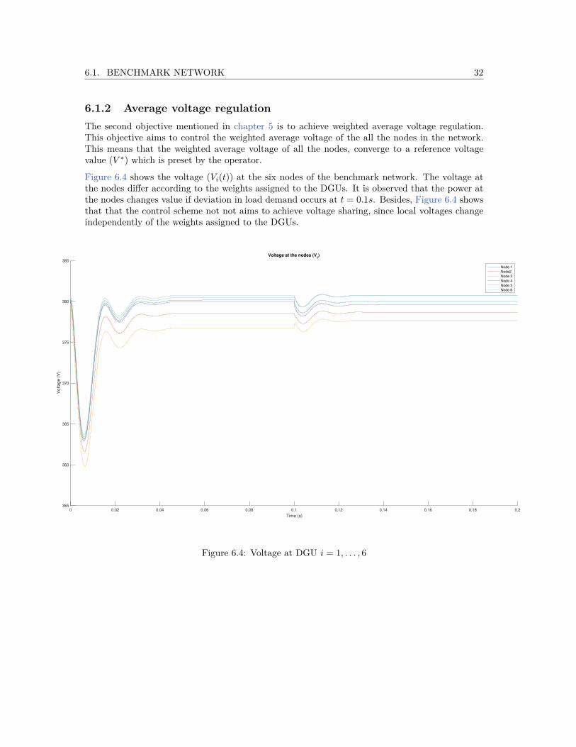
6.1.2 Average voltage regulationThe second objective mentioned in chapter 5 is to achieve weighted average voltage regulation.This objective aims to control the weighted average voltage of the all the nodes in the network.This means that the weighted average voltage of all the nodes, converge to a reference voltagevalue (V ∗) which is preset by the operator.
Figure 6.4 shows the voltage (Vi(t)) at the six nodes of the benchmark network. The voltage atthe nodes differ according to the weights assigned to the DGUs. It is observed that the power atthe nodes changes value if deviation in load demand occurs at t = 0.1s. Besides, Figure 6.4 showsthat that the control scheme not not aims to achieve voltage sharing, since local voltages changeindependently of the weights assigned to the DGUs.
0 0.02 0.04 0.06 0.08 0.1 0.12 0.14 0.16 0.18 0.2
Time (s)
355
360
365
370
375
380
385
Vo
lta
ge
(V
)
Voltage at the nodes (Vi)
Node 1
Node2
Node 3
Node 4
Node 5
Node 6
Figure 6.4: Voltage at DGU i = 1, . . . , 6

6.1. BENCHMARK NETWORK 33
However, to determine if weighted average voltage regulation in the microgrid is achieved, Fig-ure 6.5 plots the weighted average voltage of the DGUs in the network that is defined by Vavg =1>W−1V (t). Furthermore, the reference voltage (preset to 380V) is plotted, to determine if theweighted average voltage converges to the preset reference voltage value.
0 0.02 0.04 0.06 0.08 0.1 0.12 0.14 0.16 0.18 0.2
Time (s)
335
340
345
350
355
360
365
370
375
380
385
Vo
lta
ge
(V
)
Average voltage at the nodes (Vi)
(Weighted) average voltage Vavg
Reference voltage V*
Figure 6.5: Average voltage regulation
Figure 6.5 shows that at steady state the weighted average voltage Vavg converge to the referencevoltage V ∗. Therefore, weighted average voltage regulation is achieved in the benchmark network(1>W−1V = 1>W−1V ∗). After the load demand varies, the the convergence time is less, thaninitially. Also, under- and overshoot are of lower magnitude. The reason for this is that the loaddemand variation is relatively small, Therefore, the states before variation in load demand arenear the steady values.

6.2. POWER LINE FAILURE 34
6.2 Power line failureIn the second series of scenarios, failure of different power lines are simulated. There are numerousreasons that can cause power line failure in electricity network, such as damage to power cablesor joints.
A network is considered with four DGUs (n = 4), four power lines (m = 4) and three communica-tion links (mc = 4) in the following topology, with corresponding DGU parameter values describedin Table 6.4 and line parameters in Table 6.5:
Figure 6.6: A schematic representation of a four DGU microgrid network that is considered forthe simulation of the next series of scenarios
Table 6.4: DGU parameters of the four node network
DGU 1 2 3 4Lti (mH) 1.8 2.0 3.0 2.2Cti (mF) 2.2 1.9 2.5 1.7Wi (−) 0.4−1 0.2−1 0.15−1 0.25−1
V ?i (V) 380.0 380.0 380.0 380.0I∗li(0) (A) 30.0 15.0 30.0 26.0Y ∗li (0) (mS) 3.08 3.08 3.08 3.08P ∗li(0) (kW) 7.8 7.8 7.8 7.8
Table 6.5: Line parameters of the four node network
Line 1,2 2,3 3,4 4,1
Rij (mΩ) 70 50 80 60Lij (µH) 2.1 2.3 2.0 1.8

6.2. POWER LINE FAILURE 35
In the network of Figure 6.6, three identical power line failure scenarios can be identified, whichresult in ad hoc networks. Ad hoc electrical networks are formed by connecting power sourcesand loads without planning the interconnection structure (topology) in advance (Cavanagh et al.,2017). Therefore, the following three scenarios are simulated.
1. Failure of power line k41Power line k41 denotes the line connection node one and node four. This line connects twonodes, where there is no communication link between the nodes.
2. Failure of power line k12The second possible power line failure occurs when power line k12 fails. This power lineconnects two nodes where there is a communication link between the nodes (γ12). Thisscenario is identical for power lines k23 and k34
3. Failure of power lines k12 and k41 − isolation of DGU 1The third power line failure scenario occurs when two power lines fail simultaneously andisolate a node. However this DGU is not connected by power lines to the other DGUs, it stillcommunicates with DGU 2 by communication link γ12
The performance of the control scheme is investigated regarding power sharing and weightedaverage voltage regulation.

6.2. POWER LINE FAILURE 36
6.2.1 Failure of power line k41
in the first power line failure scenario, the performance of the control scheme is investigated if apower line fails, when the two nodes do not directly communicate with each other. In Figure 6.7,the power line that fails is marked in red.
Figure 6.7: Failure of power line k41
The power line failure is simulated at t = 0.1s, when the the system is initially at steady statecondition. In this scenario, the load demand does not change, as was the case during the simulationof the benchmark network in section 6.1.
The DGU parameters and line parameter can be found in Table 6.6 and Table 6.7 respectively.
Table 6.6: DGU parameters during failure of power line k41
DGU 1 2 3 4Lti (mH) 1.8 2.0 3.0 2.2Cti (mF) 2.2 1.9 2.5 1.7Wi (−) 0.4−1 0.2−1 0.15−1 0.25−1
V ?i (V) 380.0 380.0 380.0 380.0I∗li(0) (A) 30.0 15.0 30.0 26.0Y ∗li (0) (mS) 3.08 3.08 3.08 3.08P ∗li(0) (kW) 7.8 7.8 7.8 7.8
Table 6.7: Line parameters after failure of power line k41
Line 1,2 2,3 3,4
Rij (mΩ) 70 50 80Lij (µH) 2.1 2.3 2.0
6.2. POWER LINE FAILURE 37
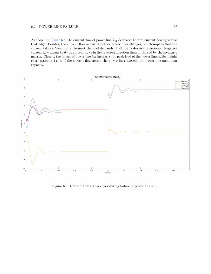
As shown in Figure 6.8, the current flow of power line k41 decreases to zero current flowing acrossthat edge. Besides, the current flow across the other power lines changes, which implies that thecurrent takes a "new route" to meet the load demands of all the nodes in the network. Negativecurrent flow means that the current flows in the reversed direction than initialised by the incidencematrix. Clearly, the failure of power line k41 increases the peak load of the power lines which mightcause stability issues if the current flow across the power lines exceeds the power line maximumcapacity.
0 0.02 0.04 0.06 0.08 0.1 0.12 0.14 0.16 0.18 0.2
Time (s)
-20
-15
-10
-5
0
5
10
15
20
25
30
Cu
rre
nt
(A)
Current flowing across edges (Iij)
Edge 1 (I12
)
Edge 2 (I23
)
Edge 3 (I34
)
Edge 4 (I41
)
Figure 6.8: Current flow across edges during failure of power line k41

6.2. POWER LINE FAILURE 38
Power sharing
In order to determine if power sharing is still achieved, Figure 6.13 shows a plot of the resultof "unweighted" power at the nodes. "Unweighted" power means that the power at each node iscompensated for its assigned weight.
0 0.02 0.04 0.06 0.08 0.1 0.12 0.14 0.16 0.18 0.2
Time (s)
-20
0
20
40
60
80
100
120
Po
we
r (k
W)
Power at (unweighted) nodes (Pi)
Node 1
Node2
Node 3
Node4
Figure 6.9: Fair power sharing among nodes during failure of power line k41
Figure 6.13 shows that power sharing is achieved if power line k41 fails during operation of themicrogrid. As expected, the control scheme requires time to find a new power consensus value.despite the power line topology, the parameters remain identical. Therefore, the unweighted powerat the nodes converge to the same power consensus value P ∗ as prior to the power line failure.

6.2. POWER LINE FAILURE 39
Average voltage regulation
In order to determine if weighted average voltage regulation is still achieved, Figure 6.10 plots theresult of the weighted average voltage of node i = 1 . . . 4 and the reference voltage V ∗ which ispreset by the operator.
0 0.02 0.04 0.06 0.08 0.1 0.12 0.14 0.16 0.18 0.2
Time (s)
335
340
345
350
355
360
365
370
375
380
385
Vo
lta
ge
(V
)
Average voltage at the nodes (Vi)
(Weighted) average voltage Vavg
Reference voltage V*
Figure 6.10: Weighted average voltage of all the nodes in the network during failure of power linek41
As shown in Figure 6.10, average voltage regulation is still achieved when power line k41 fails duringoperation. It is shown that the weighted average voltage of the nodes in the network converge tothe reference voltage. However, compared to Figure 6.5, it is observed that convergence time islonger than the constant current demand variation occurs.
6.2. POWER LINE FAILURE 40
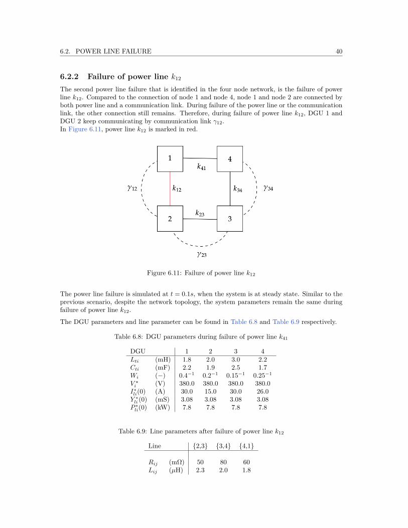
6.2.2 Failure of power line k12
The second power line failure that is identified in the four node network, is the failure of powerline k12. Compared to the connection of node 1 and node 4, node 1 and node 2 are connected byboth power line and a communication link. During failure of the power line or the communicationlink, the other connection still remains. Therefore, during failure of power line k12, DGU 1 andDGU 2 keep communicating by communication link γ12.In Figure 6.11, power line k12 is marked in red.
Figure 6.11: Failure of power line k12
The power line failure is simulated at t = 0.1s, when the system is at steady state. Similar to theprevious scenario, despite the network topology, the system parameters remain the same duringfailure of power line k12.
The DGU parameters and line parameter can be found in Table 6.8 and Table 6.9 respectively.
Table 6.8: DGU parameters during failure of power line k41
DGU 1 2 3 4Lti (mH) 1.8 2.0 3.0 2.2Cti (mF) 2.2 1.9 2.5 1.7Wi (−) 0.4−1 0.2−1 0.15−1 0.25−1
V ?i (V) 380.0 380.0 380.0 380.0I∗li(0) (A) 30.0 15.0 30.0 26.0Y ∗li (0) (mS) 3.08 3.08 3.08 3.08P ∗li(0) (kW) 7.8 7.8 7.8 7.8
Table 6.9: Line parameters after failure of power line k12
Line 2,3 3,4 4,1
Rij (mΩ) 50 80 60Lij (µH) 2.3 2.0 1.8
6.2. POWER LINE FAILURE 41
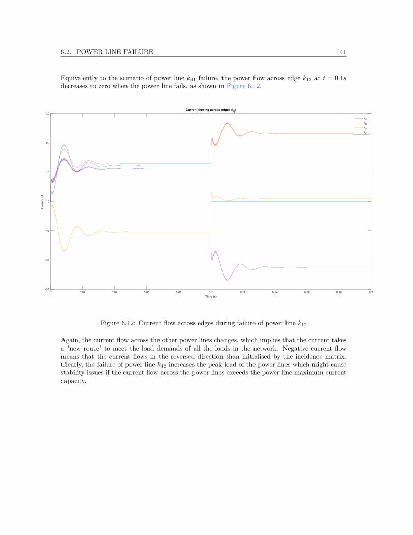
Equivalently to the scenario of power line k41 failure, the power flow across edge k12 at t = 0.1sdecreases to zero when the power line fails, as shown in Figure 6.12.
0 0.02 0.04 0.06 0.08 0.1 0.12 0.14 0.16 0.18 0.2
Time (s)
-30
-20
-10
0
10
20
30
Cu
rre
nt
(A)
Current flowing across edges (Iij)
k12
k23
k34
k41
Figure 6.12: Current flow across edges during failure of power line k12
Again, the current flow across the other power lines changes, which implies that the current takesa "new route" to meet the load demands of all the loads in the network. Negative current flowmeans that the current flows in the reversed direction than initialised by the incidence matrix.Clearly, the failure of power line k12 increases the peak load of the power lines which might causestability issues if the current flow across the power lines exceeds the power line maximum currentcapacity.

6.2. POWER LINE FAILURE 42
Power sharing
In order to determine if power sharing is still achieved, Figure 6.13 shows a plot of the resultof "unweighted" power at the nodes. "Unweighted" power means that the power at each node iscompensated for its assigned weight.
0 0.02 0.04 0.06 0.08 0.1 0.12 0.14 0.16 0.18 0.2
Time (s)
-20
0
20
40
60
80
100
120
Po
we
r (k
W)
Power at (unweighted) nodes (Pi)
Node 1
Node2
Node 3
Node 4
Figure 6.13: Fair power sharing among nodes during failure of power line k12
Figure 6.13 shows that power sharing is achieved if power line k12 fails during operation of themicrogrid. As expected, the control scheme requires time to find a new power consensus value.Despite the power line topology, the parameters remain identical. Therefore, the unweighted powerat the nodes converge to the same power consensus value P ∗ as prior to the power line failure.

6.2. POWER LINE FAILURE 43
Average voltage regulation
In order to determine if weighted average voltage regulation is still achieved, Figure 6.14 plots theresult of the weighted average voltage of node i = 1 . . . 4 and the reference voltage V ∗ which ispreset by the operator.
0 0.02 0.04 0.06 0.08 0.1 0.12 0.14 0.16 0.18 0.2
Time (s)
335
340
345
350
355
360
365
370
375
380
385
Vo
lta
ge
(V
)
Average voltage at the nodes (Vi)
(Weighted) average voltage Vavg
Reference voltage V*
Figure 6.14: Weighted average voltage of all the nodes in the network during failure of power linek12
As shown in Figure 6.14, average voltage regulation is still achieved when power line k12 failsduring operation. It is shown that the weighted average voltage of the nodes in the networkconverge to the reference voltage. Compared to Figure 6.10, it is observed that convergencestimes, undershoot- and overshoot values are approaching each other.

6.2. POWER LINE FAILURE 44
6.2.3 Failure of power line k41 and k12 − isolation of node 1In the next scenario, failure power line k41 and k12 are simulated simultaneously. In this event,DGU 1 becomes isolated, since it is not connected to the other DGUs in the network by powerlines. However, DGU 1 keeps communicating with DGU 2 through communication link γ12.In Figure 6.15, the power lines that fails are marked in red.
Figure 6.15: Failure of power line k41 and k12, which results in isolation of DGU 1
The failure of two power line is simulated simultaneously at t = 0.1s, when the system is at steadystate. As similar to the previous scenario, despite the network topology, the system parametersremain the same during failure of the power lines.It is important to mention that if a DGU is not connected to any other DGU in a network bypower lines, it is impossible to share generated power with other DGUs in a network.
The DGU parameters and line parameter can be found in Table 6.8 and Table 6.11 respectively.
Table 6.10: DGU parameters during failure of power line k41 and k12
DGU 1 2 3 4Lti (mH) 1.8 2.0 3.0 2.2Cti (mF) 2.2 1.9 2.5 1.7Wi (−) 0.4−1 0.2−1 0.15−1 0.25−1
V ?i (V) 380.0 380.0 380.0 380.0I∗li(0) (A) 30.0 15.0 30.0 26.0Y ∗li (0) (mS) 3.08 3.08 3.08 3.08P ∗li(0) (kW) 7.8 7.8 7.8 7.8
Table 6.11: Line parameters after failure of power line k41 and k12
Line 2,3 3,4
Rij (mΩ) 50 80Lij (µH) 2.3 2.0

6.2. POWER LINE FAILURE 45
Power sharing and average voltage regulation
Figure 6.16 shows a plot of the result of the voltage at PCC of nodes 1, . . . , 4. The graph showsthat at time when the two power lines fail simultaneously, the voltage at the isolated node (node1) increases to high values. As shown in the figure, the voltage at node 1 increases to over 550Vin a time span of just 0.1 seconds.On the other hand, the voltages at PCC of node 1,2 and 3 decrease after failure of power line k41and k12. It is noticed that the decrease of voltage at node 1,2 and 3 follow a similar trend as theincrease of voltage at node 1.
0 0.02 0.04 0.06 0.08 0.1 0.12 0.14 0.16 0.18 0.2
Time (s)
200
250
300
350
400
450
500
550
600
Vo
lta
ge
(V
)
Voltage at the nodes (Vi)
Node 1
Node 2
Node 3
Node 4
0.098 0.0985 0.099 0.0995 0.1 0.1005 0.101
377
378
379
380
381
382
Figure 6.16: Voltage at PCC of DGU 1, . . . , 4
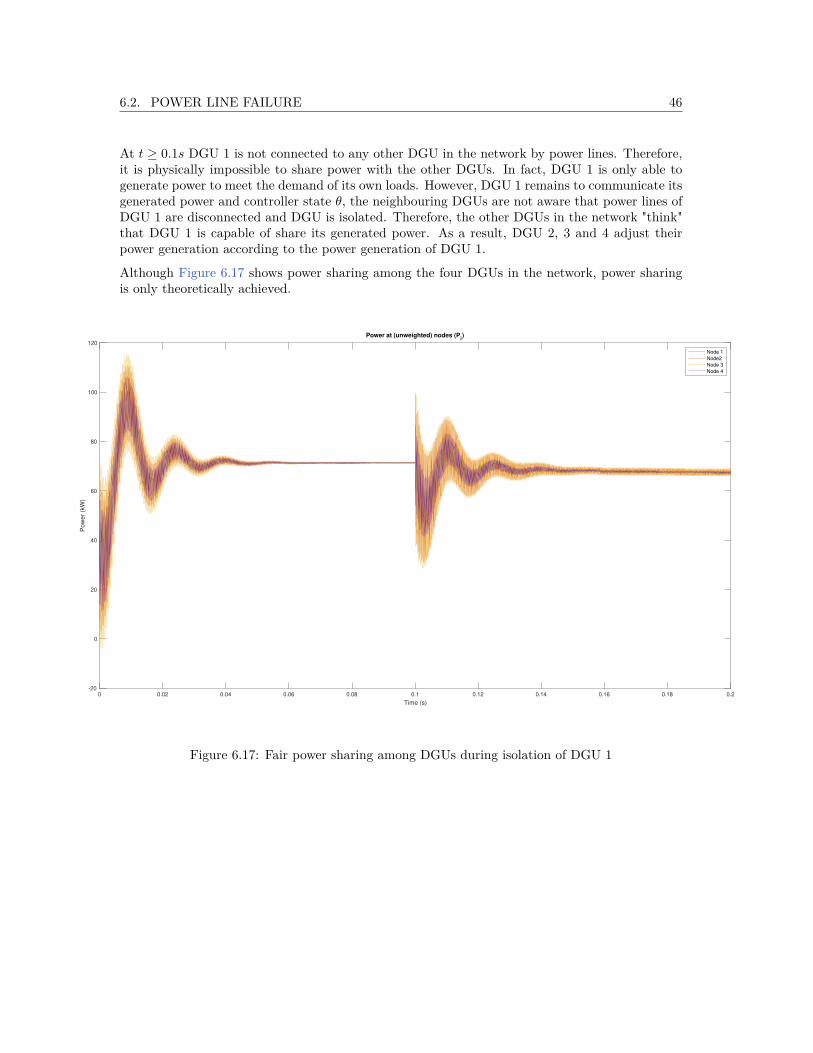
6.2. POWER LINE FAILURE 46
At t ≥ 0.1s DGU 1 is not connected to any other DGU in the network by power lines. Therefore,it is physically impossible to share power with the other DGUs. In fact, DGU 1 is only able togenerate power to meet the demand of its own loads. However, DGU 1 remains to communicate itsgenerated power and controller state θ, the neighbouring DGUs are not aware that power lines ofDGU 1 are disconnected and DGU is isolated. Therefore, the other DGUs in the network "think"that DGU 1 is capable of share its generated power. As a result, DGU 2, 3 and 4 adjust theirpower generation according to the power generation of DGU 1.
Although Figure 6.17 shows power sharing among the four DGUs in the network, power sharingis only theoretically achieved.
0 0.02 0.04 0.06 0.08 0.1 0.12 0.14 0.16 0.18 0.2
Time (s)
-20
0
20
40
60
80
100
120
Po
we
r (k
W)
Power at (unweighted) nodes (Pi)
Node 1
Node2
Node 3
Node 4
Figure 6.17: Fair power sharing among DGUs during isolation of DGU 1

6.2. POWER LINE FAILURE 47
However, to determine if weighted average voltage regulation is achieved, in Figure 6.18 the resultsare plotted of the weighted average of the four DGUs in the network together with the referencevoltage V ∗, which is preset to 380V.
0.02 0.04 0.06 0.08 0.1 0.12 0.14 0.16 0.18 0.2
Time (s)
335
340
345
350
355
360
365
370
375
380
385
Vo
lta
ge
(V
)
Average voltage at the nodes (Vi)
(Weighted) average voltage Vavg
Reference voltage V*
Figure 6.18: Weighted average voltage of all the nodes in the network
Figure 6.18 shows that the weighted average voltages of the nodes is equal to the reference valueat steady state (V = V ∗). Besides, it is observed that it takes longer to reach a consensus valueafter the isolation of node 1 and compared to the failure of one power line.

6.3. COMMUNICATION LINK FAILURE 48
6.3 Communication link failureIn this scenario, failure of communication link γ12 is simulated. It is chosen to simulate the failureof this communication line, because if the single communication link that is connected to DGU 1fails, this DGU is communicative isolated from the rest of the network. In contradiction to theprevious scenarios, no power line failure occurs.In Figure 6.19, the communication link that fails is marked in red.
Figure 6.19: Failure of communication link γ12
The failure of the communication link is simulated at t = 0.125s, when the system is at steadystate. To reach steady state after failure of communication linke γ12, the simulation runs for 5seconds. As similar to the previous scenario, despite the network topology, the system param-eters remain the same during failure of the communication line and can be found in Table 6.4andTable 6.5.

6.3. COMMUNICATION LINK FAILURE 49
Power sharing
In order to determine if power sharing is achieved among node 1, . . . , 4 if node 1 does not commu-nicate with other nodes, the result of "unweighted" power at the nodes is plotted in Figure 6.20."Unweighted" power means that the power at each node is compensated for its assigned weight.
0 0.5 1 1.5 2 2.5 3 3.5 4 4.5 5
Time (s)
-20
0
20
40
60
80
100
120
Po
we
r (k
W)
Power at (unweighted) nodes (Pi)
Node 1
Node2
Node 3
Node 4
1.23 1.235 1.24 1.245 1.25 1.255 1.26 1.265 1.27
70.8
71
71.2
71.4
71.6
71.8
Figure 6.20: Fair power sharing among all DGUs during failure of communication link γ12
Figure 6.13 shows that power sharing is among all the four DGUs is not achieved after communi-cation link γ12 fails. It is observed that DGU 1 (blue line), which is not able to communicate withother nodes, is not able to fairly share power with the other DGUs in the network that are ableto communicate. However, the unweighted power reaches a steady state value for every DGUs inthe microgrid.The underlying rationale is that the current applied to the terminals (Il) is based on the differencebetween the control input (u) and the voltage at PCC (V ) of the corresponding DGU as shownin Equation 6.1:
LtIt = −V + u (6.1)
However, the control input u applies current to the terminals according to the generated powerof the neighbouring DGUs that are exchanged via communication network (Lcomθ) as shown inEquation 6.2:
u = −K(It − φ) +WLcomθ + V ∗ (6.2)

6.3. COMMUNICATION LINK FAILURE 50
Which implies that the current applied to the terminals is not able to consider the power generatedat DGU 1 as shown in Figure 6.21, which is a plot of the current measured at the converter of DGU1, . . . , 4. This figure shows that the behaviour of the current over time at DGU 2, 3 and 4 showparallelity, because the power generated at DGU 2, 3 and 4 are exchanged over the communicationnetwork.
0 0.5 1 1.5 2 2.5 3 3.5 4 4.5 5
Time(s)
-20
0
20
40
60
80
100
120
Cu
rre
nt
(A)
Current at the nodes (Ii)
Node 1
Node 2
Node 3
Node 4
3.415 3.42 3.425
46.8
46.9
47
47.1
47.2
Figure 6.21: Measured current (It) at the converter of DGU i = 1, . . . , 4 in the network duringfailure of communication link γ12
From Figure 6.21, It is observed that the current at DGU i = 1, . . . , 4 reach steady state values.Remarkably, the measured current at DGU 1 approaches the current measured at DGU 2 at steadystate. Besides, the generated current dynamics of DGU i = 2, . . . , 4 show a linear pattern, becausethese three nodes continue communicating their injected power (i.e. generated current and voltageat PCC).

6.3. COMMUNICATION LINK FAILURE 51
Average voltage regulation
In order to determine if weighted average voltage regulation is achieved, Figure 6.10 plots theresult of the weighted average voltage of node i = 1 . . . 4 and the reference voltage V ∗ which ispreset by the operator at 380V.
0 0.5 1 1.5 2 2.5 3 3.5 4 4.5 5
Time (s)
335
340
345
350
355
360
365
370
375
380
385
Vo
lta
ge
(V
)
Average voltage at the nodes (Vi)
(Weighted) average voltage Vavg
Reference voltage V*
3.41 3.415 3.42 3.425 3.43 3.435 3.44
379.85
379.9
379.95
380
380.05
380.1
Figure 6.22: Weighted average voltage of all the nodes in the network during failure of communi-cation line γ12
As shown in Figure 6.22, average voltage regulation is when communication line γ12 fails duringoperation. It is shown that the weighted average voltage of the nodes in the network converge tothe reference voltage.The rationale that power sharing is not achieved and weighted voltage regulation is achieved whena communication link fails, is reduced from the weigthed average voltage regulation objectivefunction Equation 5.15.
To recall, at steady state φ = It. Then, the expression that describe the generated current atsteady state (It) (Equation 5.13a) results in:
0 = −V +WLcomθ + V ? (6.3)
Multiply both sides of Equation 6.3 with 1>W−1 and after rewriting, Equation 6.3 shows thatvoltage at PCC of the DGUs converge to the desired reference voltage at steady state.
1>W−1(V − V ∗) = 0 (6.4)
Equation 6.4 shows that to achieve average voltage regulation, the control scheme is not dependentof the communication network. Therefore, during failure of communication link γ12, weightedaverage voltage regulation is achieved.

6.4. PLUG-AND-PLAY 52
6.4 Plug-and-playIn this series of scenarios, the performance of the control scheme is investigated on the featureof plug-and-play in microgrids. One of the main important issues in microgrids is plug- and-play (PnP) operation of distributed generations units due to inherently discontinuous nature ofrenewable energy sources (Sadabadi et al., 2017). The concept of “plug-and-play” defines that thesystem is able to configure and integrate a component into the system by simply plugging it in.An automatic process determines the nature of the connected component to properly configureand operate (Nguyen et al., 2018).
In order to investigate the performance of the control scheme on this concept, the following twoscenarios are simulated:
1. Plug in of DGU 5In this scenario, DGU 5 is plugged into the network of four DGUs that is schematic rep-resented in Figure 6.6. DGU 5 is plugged connected to DGU 4 by a power line k45 and acommunication link γ45
2. plug out of DGU 4In this scenario, DGU 4 is plugged out of the four DGU network that is schematic representedin Figure 6.6. After DGU 4 is plugged out of the network, a three DGU network remain
The performance of the control scheme during the scenarios of plug in and plug out of DGUs, isinvestigated regarding power sharing and average voltage control regulation.

6.4. PLUG-AND-PLAY 53
6.4.1 Plug in DGU 5In this scenario, the plug in DGU 5 is simulated, including power line k45 and communication linkγ45. It is arbitrarily chosen to connect DGU 5 with DGU 4, since connecting DGU 5 to any otherDGU in the network will provide identical results.In Figure 6.23, the DGU, power line and communication link that are added are marked in green.
Figure 6.23: Plug in DGU 5
The plug in of DGU 5 simulated at t = 0.1s, when the system is at steady state. Before DGU5 is plugged it, it is assumed, that the DGU is turned off. This results in the updated microgridparameter values, where the parameters required to plug in DGU 5 are added.
The DGU parameters and line parameter can be found in Table 6.12 and Table 6.13
Table 6.12: DGU parameters when DGU 5 is plugged in.
DGU 1 2 3 4 5Lti (mH) 1.8 2.0 3.0 2.2 2.6Cti (mF) 2.2 1.9 2.5 1.7 2.1Wi (−) 0.4−1 0.2−1 0.15−1 0.25−1 0.3−1
V ?i (V) 380.0 380.0 380.0 380.0 380.0I∗li(0) (A) 30.0 15.0 30.0 26.0 28.0Y ∗li (0) (mS) 3.08 3.08 3.08 3.08 3.08P ∗li(0) (kW) 7.8 7.8 7.8 7.8 7.8
Table 6.13: Line parameters after DGU 5 is plugged in
Line 1,2 2,3 3,4 4,1 4,5
Rij (mΩ) 70 50 80 60 70Lij (µH) 2.1 2.3 2.0 1.8 1.9

6.4. PLUG-AND-PLAY 54
Power sharing
In order to determine if power sharing is achieved between all the DGUs in the network, Figure 6.24plots the results of unweighted power at the nodes. "Unweighted" power means that the power ateach node is compensated for its assigned weight.
0 0.02 0.04 0.06 0.08 0.1 0.12 0.14 0.16 0.18 0.2
Time (s)
-20
0
20
40
60
80
100
120
Po
we
r (k
W)
Power at (unweighted) nodes (Pi)
Node 1
Node2
Node 3
Node 4
Node 5
Figure 6.24: Fair power sharing among all DGUs during plug in of DGU 5
Figure 6.24 shows that power sharing is achieved among the DGUs in the network, even when aDGU is plugged in. The graph shows that the power at DGU 5 is zero during during the firsttime span, as it is plugged at t = 0.1. Until t = 0.1, DGU 5 is assumed to be turned off, whichresult in zero power generation. As expected, the control scheme requires time to find a new powerconsensus value. Depending on the weight that is assigned to the DGU, the new power consensusvalue differs from the power consensus value of the network topology prior to the plug in of DGU5.

6.4. PLUG-AND-PLAY 55
Average voltage regulation
In order to determine if weighted average voltage regulation is still achieved, Figure 6.25 plotsthe result of the weighted average voltage of DGU i = 1, . . . , 4 for 0 ≤ t < 0.1s and the weightedaverage voltage of DGU i = 1, . . . , 5 for 0.1 ≤ t ≤ 0.2s the reference voltage V ∗ which is preset bythe operator.
0 0.02 0.04 0.06 0.08 0.1 0.12 0.14 0.16 0.18 0.2
Time (s)
335
340
345
350
355
360
365
370
375
380
385
Vo
lta
ge
(V
)
Average voltage at the nodes (Vi)
(Weighted) average voltage Vavg
Reference voltage V*
Figure 6.25: Weighted average voltage of connected nodes in the network
As shown in Figure 6.25, average voltage regulation is still achieved if DGU is plugged in duringoperation. It is shown that the weighted average voltage of the nodes in the network converge tothe reference voltage. At steady state V = V ∗.

6.4. PLUG-AND-PLAY 56
6.4.2 Plug out DGU 4In this scenario, the plug out DGU 4 is simulated, including power lines k41, k34 and communicationlink γ34. DGUs are plugged out of the microgrid for various reasons (e.g. maintenance purposes).It is chosen to plug out DGU 4, since this DGU is connect identical connected to two nodes. DGU4 is connected to DGU 3 by a power line and a communication link, while it is connected to DGU1 by only a power line.In Figure 6.26, the network topology of the network after plug out DGU 4 is schematic represented.
Figure 6.26: Plug out DGU 4
The plug out of DGU 4 simulated at t = 0.1s, when the system is at steady state. When DGU4 is plugged out, it is assumed, that the DGU is turned off. As similar to the previous scenarios,despite the network topology, the system parameters remain the same during plug out of DGU 4.
The DGU parameters and line parameter can be found in Table 6.14 and Table 6.15
Table 6.14: DGU parameters after DGU 4 is plugged out
DGU 1 2 3Lti (mH) 1.8 2.0 3.0Cti (mF) 2.2 1.9 2.5Wi (−) 0.4−1 0.2−1 0.15−1
V ?i (V) 380.0 380.0 380.0I∗li(0) (A) 30.0 15.0 30.0Y ∗li (0) (mS) 3.08 3.08 3.08P ∗li(0) (kW) 7.8 7.8 7.8
Table 6.15: Line parameters after DGU 4 is plugged out
Line 1,2 2,3
Rij (mΩ) 70 50Lij (µH) 2.1 2.3

6.4. PLUG-AND-PLAY 57
Power sharing
In order to determine if power sharing is achieved between all the DGUs in the network, Figure 6.27plots the results of unweighted power at the nodes. "Unweighted" power means that the power ateach node is compensated for its assigned weight.
0 0.02 0.04 0.06 0.08 0.1 0.12 0.14 0.16 0.18 0.2
Time (s)
-20
0
20
40
60
80
100
120
Po
we
r (k
W)
Power at (unweighted) nodes (Pi)
Node 1
Node2
Node 3
Node 4
Figure 6.27: Fair power sharing among all DGUs during plug in of DGU 5
Figure 6.24 shows that power sharing is achieved among the DGUs in the network, even when anadditional DGU is plugged in. The graph shows that the power at DGU 5 is zero during duringthe first time span, as it is plugged at t = 0.1. From t = 0.1, DGU 4 is assumed to be turnedoff, which result in zero power generation. Therefeore, the unweighted power at DGU 4 is zerofor t ≥ 0.1s. As expected, the control scheme requires time to find a new power consensus value.However, the convergence of the unweighted power to the consensus value is relatively fast, withminimum under- and overshoot.

6.4. PLUG-AND-PLAY 58
Average voltage regulation
In order to determine if weighted average voltage regulation is still achieved, Figure 6.28 plotsthe result of the weighted average voltage of DGU i = 1, . . . , 4 for 0 ≤ t < 0.1s and the weightedaverage voltage of DGU i = 1, . . . , 3 for 0.1 ≤ t ≤ 0.2s, since DGU 4 is plugged out and assumedturned off for t ≥ 0.1s. Furthermore, the reference voltage V ∗ is plotted, which is preset by theoperator.
0 0.02 0.04 0.06 0.08 0.1 0.12 0.14 0.16 0.18 0.2
Time (s)
335
340
345
350
355
360
365
370
375
380
385
Vo
lta
ge
(V
)
Average voltage at the nodes (Vi)
(Weighted) average voltage Vavg
Reference voltage V*
Figure 6.28: Weighted average voltage of connected nodes in the network
As shown in Figure 6.25, average voltage regulation is still achieved if DGU 4 is plugged out duringoperation. It is shown that the weighted average voltage of the nodes in the network converge tothe reference voltage. At steady state V = V ∗.

6.5. INTERPRETATION OF RESULTS 59
6.5 Interpretation of resultsSubsequent to the results of the extensive simulation of the control scheme to investigate its per-formance in critical scenarios, the results are interpreted in this section, which leads to importantinsights of the proposed controller regarding the design of microgrids.
Firstly, it can be concluded that the general performance of the control scheme is promising. Thecontrol scheme achieves fair power sharing among all the DGUs in a network and weighted averagepower sharing simultaneously in regular circumstances as shown by simulating the DC microgridbenchmark network. The proposed control scheme is robust to load demand variation, which isan ordinary circumstance during the operation of a DC microgrid.Besides, it turned out that the control scheme is robust to power line failure in the network, sincethree different power line failure scenarios are simulated. During all three cases, fair power sharingand average voltage are theoretically achieved. When one power line fails in the system, the resultshows that current flows through other power lines to meet load demands and achieve the controlobjectives, which is desired performance. However, during simultaneously failure of two powerlines which results in isolation of a DGU, fair power sharing and average voltage regulation istheoretically achieved, but is impossible in reality. The reason behind this is that if a DGU isisolated by power lines, it is able to generate power to meet its own load demands, but unableto share its generated power. However, if the isolated DGU continue to communicate with otherDGUs in the network, the controller will not notice that the DGU is isolated and not able to shareits generated power.This behaviour of the proposed control scheme is supported by the simulation of a communicationlink failure scenario. The result of the simulation shows that during the failure of a communicationlink, the controller is unable to achieve fair power sharing since to achieve this objective, the controlscheme requires information about the power that is injected at neighbouring DGU. On the otherhand, weighted average voltage regulation is achieved, since to achieve this objective, the controlscheme does not rely on the state of the communication network. Besides, it is observed thatthe voltage at PCC of the DGU that is isolated, increases heavily. It is needless to say that thisbehaviour is undesirable since it can cause stability and safety issues.
The rationale behind this behaviour is found in the design of the control scheme. Namely, themicrogrid is controlled in a distributed manner. This implies that no central controller is requiredand local controllers share information over a communication network. This concept is used todesign the control scheme that is proposed in this research, where control states are shared via acommunication network (Lcomθ) as shown in Equation 5.12. The control input of a DGU is purelydependent on its own states and its neighbours states, which are exchanged by the communicationnetwork. Therefore power line failure, which results in isolation of a DGU or a cluster of DGUs,remains unnoticed and causes undesirable behaviour. Also, it is shown that every DGU must beconnected to at least one other DGU. In the four DGU network that is used during simulation,some DGUs are connected in the communication network by a single communication link, whichdenotes that in this network, the control scheme is not immune to a single point of failure (SPOF).
The analysis of the simulation results leads to interesting insights regarding the design of a mi-crogrid system. Although the performance of the control scheme is promising, some importantaspects should be taken into consideration to ensure the safety and stability of a DC microgrid. Itis advisable to obtain knowledge of the state of the power lines and communication links duringall times. It is essential for the proper operation of the microgrid and its controllers that DGUs ina network are prevented for communicative isolation or power flow isolation. Isolation of DGUs ina microgrid network should directly be noticed (e.g. by sensors) to prevent power outages in thenetwork. If a DGU is isolated by power line failure, the DGU must be plugged out of the network,to disconnect communication between the isolated DGU and the rest of the network. Similarly,if a DGu is communicatively isolated, it should stop generating power to prevent undesirablebehaviour of the DGU in the microgrid network.

6.5. INTERPRETATION OF RESULTS 60

Chapter 7
Conclusion
In this chapter research question 8 is addressed. This chapter determines the main conclusions ofthe thesis to add knowledge to existing literature. In this thesis, a distributed control scheme isproposed that achieves power sharing and average voltage regulation in DC microgrids to increasethe stability and reliability of the power system. Besides, The performance of the proposedcontrol scheme is investigated by simulation of critical scenarios that eventually happen in DCmicrogrids. Analysis of the results provides an appropriate performance indication and leads tointeresting insights regarding the design of microgrids. Although the DC microgrid model thatis used is fairly standard, the proposed control scheme shows some unique benefits over controlschemes that are proposed in literature. which enhances the applicability of the proposed controlscheme to control DC microgrids.
From the simulation study, it is concluded that the performance of the controller is promising.Under regular circumstances, fair power sharing and average voltage regulation are achieved si-multaneously in various network topologies. Also, the proposed control scheme shows good per-formance in controlling a DC microgrid benchmark network.As shown for two cases, the distributed control scheme is capable of handling power line failurein DC microgrids if the power line failure does not result in isolation of a DGU. Due to the prop-erty of DC microgrids that the communication network can differ from the power line networktopology, three identical power line failures are identified in a four DGU microgrid. The resultsshow that current flow via different power lines if a single power line fails to remain power sharingin the network. However, due to the design of the control scheme, to achieve power sharing, aDGU is dependent of its states, but also on a control state and the power that is injected atits neighbours. This information is shared via a communication network. Therefore, the controlscheme only achieves fair power sharing and average voltage regulation if it receives the correctinformation from its neighbours. Due to this limitation, it is shown that power sharing is notachieved when failure of power line(s) results in the isolation of a DGU. A simulation is conductedwhere two power lines fail simultaneously and cause isolation of a DGU. The result shows thatthe controller’s two objectives are not achieved. The reason is that isolated DGU keeps commu-nicating its states to its neighbours when it is isolated. Therefore, the isolation of a DGU is notnoticed, and the control scheme aims to share power between all the DGUs in the network, whichis physically impossible.Furthermore, the simulation of communication link failure endorses the vital role of the com-munication network in the control scheme to achieve power sharing. During the simulation of acommunication link failure, a DGU became communicatively isolated, which means that it wasnot connected to any other DGU by a communication line. In this scenario, fair power sharing isnot achieved. On the other hand, due to the design of the control scheme, the state of the commu-nication network is does not affect the regulation of weighted average voltage. Therefore, if a DGUbecomes communicatively isolated, weighted average voltage regulation will still be achieved.
61

62
The analysis of the simulation results leads to interesting insights regarding the design of mi-crogrids. During the isolation of a DGU, the voltages level of that DGU increases to criticallevels which decreases the safety and reliability of the power system. Therefore, the state of thepower lines and communication lines should be monitored during all operation times to preventthe failure of power lines and communication links that result in the isolation of DGUs in themicrogrid network. Sensors can be installed to measure the current flow across power lines todetect any failure of the power lines. If isolation of DGUs is directly noticed, corresponding DGUscan be plugged out of the network, or the power generation of the isolated DGU can be stoppedto maintain power sharing and average voltage regulation in DC microgrids.

Chapter 8
Limitations and further research
The purpose of this chapter is to discuss the limitations of the current research, and put theminto perspective for further research. It cannot be emphasized enough that the range of possibili-ties and approaches, in performing research on controlling and stabilizing dynamical networks asmicrogrids, is extraordinary. Many more research directions can be taken. This thesis providesthe results of one strategy to control DC microgrids, but further research is necessary in order toimplement this prospective grid in the future.
First of all, most of the parameters used in the current simulation studies, including load parame-ters, line parameters and DGU parameters, were adopted from other references such as Weitenberg(2018), Trip et al. (2018), De Persis et al. (2018). Due to the limited time span of the this study,validation of the large number of system parameters was not possible. In future research, thiscould be further investigated, by theoretical or empirical justification of the parameters and inputdata for specific microgrids.Secondly, it would be interesting to extend the simulations by including scenarios, or apply thecontrol algorithm to AC or hybrid microgrids, to investigate the performance of this control schemein larger networks or AC microgrids. In literature, many current and power sharing methods areproposed (Han et al. (2017), Nasirian et al. (2014), Anand et al. (2012) and Zhao and Dörfler(2015)). Also, the voltage balancing problem is adressed in literature (Tucci et al. (2018) Nasirianet al. (2014)) An comparative evaluation of the control scheme performance that is proposed inthis thesis with a control scheme proposed in literature would be a interesting for further researchto obtain a better performance indication of the proposed control scheme.
Furthermore, the model can be further extended by including more dynamics. In the DC microgridmodel that is developed in this research, the sources are considered to be controllable distributedgeneration units. The DGUs are constant power sources. However, renewable energy sources (e.g.solar, wind and tidal) are usually sources that are adopted in DC microgrid. These sources donot deliver constant power continuously, due to intermittent of nature (Shivashankar et al., 2016).Therefore, including power source dynamics would be an interesting extension which increase thecomplexity.Besides, in the DC microgrid model that is considered in this work, a buck converter is used tostep down voltage (while stepping up current) from its input (supply) to its output (load). Insteadof a buck converter, buck-boost or boost converters can be considered, since boost converters aremore desirable for PV sources. The dynamics of the DC microgrid model can be extended byincluding dynamics of the converter, which are nonlinear. (Cucuzzella et al., 2019c).
63

64
The last and most important limitation of this research is that a theoretical validation of theproposed control scheme is lacking. The conclusions regarding the performance of the controlscheme are solely based on a simulation study. Although the control scheme shows promisingperformance during simulation, definite conclusions of the performance can not be given due tothe lack of theoretical validation.In order to validate the control scheme, the stability of the dynamical system must be proven.Stability is the most commonly studied property of invariant sets. Roughly speaking, an invariantset is called stable if trajectories starting close to it remain close to it, and unstable if they do not(Lestas, 2019). In this work, it is assumed that an equilibrium exist and that (It, V , I, Tθ, Tφ)always converge to a steady state solution (It, V , I, Tθ, Tφ). Lyapunov theory is fundamental insystems theory (Kosaraju et al., 2018). By applying Lyapunov’s direct method, stability of thedynamical system can be proven by finding a positive definite differential Lyapunov function, ofwhich its derivative is semi-definite. If such a suitable Lyapunov candidate is found, the stabilityof the system dynamics can be proven.

Bibliography
Anand, S., Fernandes, B. G., and Guerrero, J. (2012). Distributed control to ensure proportionalload sharing and improve voltage regulation in low-voltage dc microgrids. IEEE transactionson power electronics, 28(4):1900–1913.
Arif, M. S. B. and Hasan, M. A. (2018). Microgrid architecture, control, and operation. InHybrid-Renewable Energy Systems in Microgrids, pages 23–37. Elsevier.
Beykverdi, M., Jalilvand, A., and Ehsan, M. (2017). Decentralized control of low-voltage islandeddc microgrid using power management strategies. American Journal of Science, Engineeringand Technology, 1(2):27.
Cavanagh, K., Belk, J. A., and Turitsyn, K. (2017). Transient stability guarantees for ad hoc dcmicrogrids. IEEE Control Systems Letters, 2(1):139–144.
Conejo, A. J. and Baringo, L. (2018). Power system operations. Springer.
Cucuzzella, M., Incremona, G. P., and Ferrara, A. (2017). Decentralized sliding mode control ofislanded ac microgrids with arbitrary topology. IEEE Transactions on Industrial Electronics,64(8):6706–6713.
Cucuzzella, M., Kosaraju, K. C., and Scherpen, J. (2019a). Voltage control of dc networks:robustness for unknown zip-loads. arXiv preprint arXiv:1907.09973.
Cucuzzella, M., Kosaraju, K. C., and Scherpen, J. M. (2019b). Distributed passivity-based controlof dc microgrids. In 2019 American Control Conference (ACC), pages 652–657. IEEE.
Cucuzzella, M., Lazzari, R., Kawano, Y., Kosaraju, K. C., and Scherpen, J. M. (2019c). Robustpassivity-based control of boost converters in dc microgrids. In 2019 IEEE 58th Conference onDecision and Control (CDC), pages 8435–8440. IEEE.
Cucuzzella, M., Lazzari, R., Trip, S., Rosti, S., Sandroni, C., and Ferrara, A. (2018a). Sliding modevoltage control of boost converters in dc microgrids. Control Engineering Practice, 73:161–170.
Cucuzzella, M., Trip, S., De Persis, C., Cheng, X., Ferrara, A., and van der Schaft, A. (2018b). Arobust consensus algorithm for current sharing and voltage regulation in dc microgrids. IEEETransactions on Control Systems Technology, 27(4):1583–1595.
Datta, U., Kalam, A., and Shi, J. (2018). Hybrid pv–wind renewable energy sources for microgridapplication: an overview. In Hybrid-Renewable Energy Systems in Microgrids, pages 1–22.Elsevier.
De Persis, C., Weitenberg, E. R., and Dörfler, F. (2018). A power consensus algorithm for dcmicrogrids. Automatica, 89:364–375.
de Souza, A. C. Z. and Castilla, M. (2019). Microgrids Design and Implementation. Springer.
DENA (2019). Energy Transition Trends 2019. https://www.dena.de/fileadmin/dena/
65

BIBLIOGRAPHY 66
Dokumente/Themen_und_Projekte/Internationales/China/CREO/Energy_transition_trends_2019_engl.pdf.
Dorfler, F. and Bullo, F. (2012). Kron reduction of graphs with applications to electrical networks.IEEE Transactions on Circuits and Systems I: Regular Papers, 60(1):150–163.
EPA (2018a). Centralized Generation of Electricity and its Im-pacts on the Environment. https://www.epa.gov/energy/centralized-generation-electricity-and-its-impacts-environment.
EPA (2018b). Distributed Generation of Electricity andits Environmental Impacts. https://www.epa.gov/energy/distributed-generation-electricity-and-its-environmental-impacts.
Fei, G., Ren, K., Jun, C., and Tao, Y. (2019). Primary and secondary control in dc microgrids: areview. Journal of Modern Power Systems and Clean Energy, 7(2):227–242.
Guerrero, J. M., Chandorkar, M., Lee, T.-L., and Loh, P. C. (2012a). Advanced control ar-chitectures for intelligent microgrids—part i: Decentralized and hierarchical control. IEEETransactions on Industrial Electronics, 60(4):1254–1262.
Guerrero, J. M., Loh, P. C., Lee, T.-L., and Chandorkar, M. (2012b). Advanced control architec-tures for intelligent microgrids—part ii: Power quality, energy storage, and ac/dc microgrids.IEEE Transactions on Industrial Electronics, 60(4):1263–1270.
Han, R., Meng, L., Guerrero, J. M., and Vasquez, J. C. (2017). Distributed nonlinear controlwith event-triggered communication to achieve current-sharing and voltage regulation in dcmicrogrids. IEEE Transactions on Power Electronics, 33(7):6416–6433.
Incremona, G. P., Cucuzzella, M., and Ferrara, A. (2016). Adaptive suboptimal second-ordersliding mode control for microgrids. International Journal of Control, 89(9):1849–1867.
ISGF (2019). Distributed generation. http://www.indiasmartgrid.org/Distributed-Generation.php.
Jerin, A. R. A., Prabaharan, N., Kumar, N. M., Palanisamy, K., Umashankar, S., and Siano,P. (2018). 10 - smart grid and power quality issues. In Fathima, A. H., Prabaharan, N.,Palanisamy, K., Kalam, A., Mekhilef, S., and Justo, J. J., editors, Hybrid-Renewable EnergySystems in Microgrids, Woodhead Publishing Series in Energy, pages 195 – 202. WoodheadPublishing.
Justo, J. J., Mwasilu, F., Lee, J., and Jung, J.-W. (2013). Ac-microgrids versus dc-microgrids withdistributed energy resources: A review. Renewable and sustainable energy reviews, 24:387–405.
Kosaraju, K. C., Cucuzzella, M., Scherpen, J., and Pasumarthy, R. (2018). Differentiation andpassivity for control of brayton-moser systems. arXiv preprint arXiv:1811.02838.
Lasseter, R. H. and Piagi, P. (2004). Microgrid: A conceptual solution. In IEEE Power ElectronicsSpecialists Conference, volume 6, pages 4285–4291. Citeseer.
Leonard, J. P. (2014). Nonlinear modeling of dc constant power loads with frequency domainvolterra kernels.
Lestas, I. (2019). Handout 2: Invariant sets and stability. http://www2.eng.cam.ac.uk/~icl20/4f3/Handout2.pdf.
Lotfi, H. and Khodaei, A. (2015). Ac versus dc microgrid planning. IEEE Transactions on SmartGrid, 8(1):296–304.
Mirakhorli, A. and Dong, B. (2016). Occupancy behavior based model predictive control forbuilding indoor climate—a critical review. Energy and Buildings, 129:499–513.
BIBLIOGRAPHY 67
Nasirian, V., Moayedi, S., Davoudi, A., and Lewis, F. L. (2014). Distributed cooperative controlof dc microgrids. IEEE Transactions on Power Electronics, 30(4):2288–2303.
Nguyen, T.-L., Guillo-Sansano, E., Syed, M. H., Nguyen, V.-H., Blair, S. M., Reguera, L., Tran,Q.-T., Caire, R., Burt, G. M., Gavriluta, C., et al. (2018). Multi-agent system with plug andplay feature for distributed secondary control in microgrid—controller and power hardware-in-the-loop implementation. Energies, 11(12):3253.
O’gorman, R. and Redfern, M. (2004). Voltage control problems on modern distribution systems.In IEEE Power Engineering Society General Meeting, 2004., pages 662–667. IEEE.
Olivares, D. E., Mehrizi-Sani, A., Etemadi, A. H., Cañizares, C. A., Iravani, R., Kazerani, M.,Hajimiragha, A. H., Gomis-Bellmunt, O., Saeedifard, M., Palma-Behnke, R., et al. (2014).Trends in microgrid control. IEEE Transactions on smart grid, 5(4):1905–1919.
Papathanassiou, S., Hatziargyriou, N., Strunz, K., et al. (2005). A benchmark low voltage micro-grid network. In Proceedings of the CIGRE symposium: power systems with dispersed generation,pages 1–8. CIGRE.
Perez, F. and Damm, G. (2019). Dc microgrids. In Microgrids Design and Implementation, pages447–475. Springer.
Rahmani, S., Saeidi, M., and Pirayesh, A. (2017). A combinational power sharing strategy basedon master-slave and droop methods for power-electronics-interfaced distributed generation unitsoperating in a dc micro-grid. In 2017 IEEE International Conference on Smart Energy GridEngineering (SEGE), pages 1–6. IEEE.
Rinaldi, G., Cucuzzella, M., and Ferrara, A. (2017). Third order sliding mode observer-based ap-proach for distributed optimal load frequency control. IEEE Control Systems Letters, 1(2):215–220.
Sadabadi, M. S., Shafiee, Q., and Karimi, A. (2017). Plug-and-play robust voltage control of dcmicrogrids. IEEE Transactions on Smart Grid, 9(6):6886–6896.
Saleh, M., Esa, Y., and Mohamed, A. A. (2018). Communication-based control for dc microgrids.IEEE Transactions on Smart Grid, 10(2):2180–2195.
Setiawan, M. A., Abu-Siada, A., and Shahnia, F. (2016a). New technique for power sharing in dcmicrogrids. In 2016 IEEE 2nd Annual Southern Power Electronics Conference (SPEC), pages1–5. IEEE.
Setiawan, M. A., Abu-Siada, A., and Shahnia, F. (2016b). Voltage regulation in dc microgridswith various circuit configurations. In 2016 IEEE 2nd Annual Southern Power ElectronicsConference (SPEC), pages 1–6. IEEE.
Shivashankar, S., Mekhilef, S., Mokhlis, H., and Karimi, M. (2016). Mitigating methods of powerfluctuation of photovoltaic (pv) sources–a review. Renewable and Sustainable Energy Reviews,59:1170–1184.
Su, W., Wang, J., and Roh, J. (2013). Stochastic energy scheduling in microgrids with intermittentrenewable energy resources. IEEE Transactions on Smart grid, 5(4):1876–1883.
Trip, S., Bürger, M., and De Persis, C. (2014). An internal model approach to frequency regulationin inverter-based microgrids with time-varying voltages. In 53rd IEEE Conference on Decisionand Control, pages 223–228. IEEE.
Trip, S., Cucuzzella, M., Cheng, X., and Scherpen, J. (2018). Distributed averaging controlfor voltage regulation and current sharing in dc microgrids. IEEE Control Systems Letters,3(1):174–179.

BIBLIOGRAPHY 68
Trip, S., Cucuzzella, M., De Persis, C., Ferrara, A., and Scherpen, J. M. (2020). Robust loadfrequency control of nonlinear power networks. International Journal of Control, 93(2):346–359.
Tucci, M., Meng, L., Guerrero, J. M., and Ferrari-Trecate, G. (2018). Stable current sharing andvoltage balancing in dc microgrids: A consensus-based secondary control layer. Automatica,95:1–13.
Venkatraman, R. and Khaitan, S. K. (2015). A survey of techniques for designing and managingmicrogrids. In 2015 IEEE Power & Energy Society General Meeting, pages 1–5. IEEE.
Wang, Z., Liu, F., Chen, Y., Low, S. H., and Mei, S. (2017). Unified distributed control ofstand-alone dc microgrids. IEEE Transactions on Smart Grid, 10(1):1013–1024.
Weitenberg, E. (2018). Control of electrical networks: robustness and power sharing.
Zhao, J. and Dörfler, F. (2015). Distributed control and optimization in dc microgrids. Automatica,61:18–26.

Appendix A
Benchmark network
A.1 Benchmark LV microgrid network
Figure A.1: Benchmark LV microgrid network (Papathanassiou et al., 2005)
69

A.2. REDUCED BENCHMARK LV MICROGRID NETWORK 70
A.2 Reduced benchmark LV microgrid network
Figure A.2: Reduced benchmark LV microgrid network (Wang et al., 2017)