scalable dc microgrids for rural electrification

i

Scalable DC Microgrids for Rural

Electrification

A Dissertation

Presented by

MASHOOD NASIR

In partial fulfillment

of the requirements for the degree of

Doctor of Philosophy

in Electrical Engineering

Supervisor: Hassan Abbas Khan (LUMS)

Co-supervisor: Nauman Ahmad Zaffar (LUMS)

Syed Babar Ali School of Sciences and Engineering

Lahore University of Management Sciences (LUMS)

Lahore, Pakistan.

ii

Dedicated to the service of humanity and the noble cause of energy

poverty eradication

iii

Acknowledgement

The author expresses his gratitude, appreciation and sincere thanks

to his supervisor Dr. Hassan Abbas khan and co-supervisor Prof.

Nauman Ahmad Zaffar for their supervision of this research work.

Their advice, guidance and assistance, both technical and financial

in conducting this research and the preparation of this thesis are

thankfully acknowledged.

The author is extremely thankful to his foreign supervisor Prof.

Josep M. Guerrero and co-supervisor Juan C.Vasquez, who guided

and helped him conducting part of this research during his stay at

Aaalborg University (AAU), Denmark.

The author also thanks the advisory committee members including

Dr. Naveed-ul-Hassan, Dr. Jahangir Ikram for their suggestions

and advice. The author would also lie thank to external evaluator

Dr. Tauseef Tauqeer and internal evaluator Dr. Naveed Arshad for

their constructive remarks.

Assistance provided by the colleagues at EPS cluster, lab staff

including M. Farman Ali and Secretarial staff of the SBASSE is

thankfully acknowledged.

The author also acknowledges his parents, brothers and sister for

their prayers, constant encouragement and loving support

throughout his study tenure. Last but not the least; author would

like to thank his beloved wife for always being a constant source of

inspiration and support during this work.

iv

Abstract

Access to electricity is one of the key factors indicating the socio-economic status

of any community. Reliable and adequate provision of electricity is mandatory for

improved standards of living including better health, education, transport, agriculture and

employment opportunities. Unfortunately, according to International Energy Agency,

over 1.1 billion people around the world lack access to any electricity out of which 85

percent reside in rural areas of developing world. Electrification of these remote rural

communities through national grid interconnection is not economically feasible for many

developing countries due to high cost associated with the development of generation,

transmission and distribution infrastructure. Alternatively, DC microgrids implemented

with distributed generation and low voltage distribution are becoming very popular for

low cost rural electrification. However, current implementations are largely suboptimal

due to high distribution losses associated with their centralized architecture and their

inability to support high power community loads. In this work, a novel distributed DC

microgrid architecture which allows a scalable approach with minimal upfront investment

to fulfill rural electricity needs along with the provision of higher powers for communal

loads and beyond subsistence provisioning of electrical power is proposed. The

architecture is capable to work entirely on solar energy with power delivery capability to

individual consumers and added inherent ability to integrate resources to power up larger

loads for communal/commercial applications. The proposed microgrid architecture

consists of a cluster of multiple nanogrids (households), where each nanogrid has its own

PV generation and battery storage along with bi-directional connectivity to the microgrid.

Thus, each nanogrid can work independently in islanded mode along with the provision

of sharing its resources with the community through the bidirectional converter. In the

proposed architecture, the bi-directional power flow capability is implemented through a

modified flyback converter. A decentralized control methodology is also proposed to

ensure a communication-less, yet coordinated control among the distributed resources in

multiple nanogrids. The microgrid is evaluated for optimal distribution voltage level,

conductor size and interconnection scheme between nanogrids using Newton-Raphson

analysis modified for DC power flow. Various scenarios for power sharing among the

contributing nanogrids and communal load power allocation are analyzed from operation

and control prospective to validate the architecture and its performance. Further, an

optimal framework for the planning of distributed generation and storage resources in

each nanogrid with respect to time varying profiles of region-specific temperature and

irradiance is also presented to ensure the better resource utilization. A scaled version of

the proposed architecture is implemented on hardware, while the efficacy of control

methodology is validated on MATLAB/Simulink and hardware in loop facilities at

microgrid laboratory in Aalborg University. The proposed distributed architecture along

with decentralized control can be considered as a promising solution for the future rural

electrification implementations in developing regions.

v

List of Publications from thesis work

Journal Articles

[J1]. M. Nasir, H. A. Khan, A. Hussain, L. Mateen, and N. A. Zaffar, "Solar PV-Based

Scalable DC Microgrid for Rural Electrification in Developing Regions," IEEE

Transactions on Sustainable Energy, vol. 9, pp. 390-399, 2018.

http://ieeexplore.ieee.org/document/8002658/

[J2]. M. Nasir, S. Iqbal, and H. A. Khan, "Optimal Planning and Design of Low-Voltage

Low-Power Solar DC Microgrids," IEEE Transactions on Power Systems, vol. 33, issue

33, pp. 2919-2928, 2018.


[J3]. M. Nasir, Z. Jin, Hassan A. Khan, N. Zaffar, J.C. Vasquez, J. M. Guerrero, "A

Decentralized Control Architecture applied to DC Nanogrid Clusters for Rural

Electrification in Developing Regions." IEEE Transactions on Power Electronics, 2018.

https://ieeexplore.ieee.org/document/8341807/

[J4]. H. A. Khan, H. F. Ahmad, N. A. Zaffar, M. F. Nadeem and M. Nasir, "Decentralized

Electric Power Delivery Model for Rural Electrification in Pakistan, ", Under Revision,

Energy Policy.

Conference Proceedings

[C1]. M. Nasir, N. A. Zaffar, and H. A. Khan, "Analysis on central and distributed

architectures of solar powered DC microgrids," in Clemson University Power Systems

Conference (PSC), 2016, pp. 1-6.


[C2]. M. S. M. Hamza, S. Fazal, M. Nasir and H. Khan, "Design and Analysis of Solar PV

based Low-Power Low-Voltage DC Microgrid Architectures for Rural Electrification,"

IEEE PES General Meeting, Energizing a More Secure, Resiliant and Adaptable Grid,

Chicago, IL USA, 2017. http://ieeexplore.ieee.org/document/8274134/

[C3]. M. Nasir, H. A. Khan, Z. Jin amd J. M. Guerrero, "Dual–loop Control Strategy applied

to PV/battery based Islanded DC microgrids for Swarm Electrification of Developing

Regions," IET, Renewable Power Generation conference (RPG), Copenhagen, Denmark

2018.

Working Papers

M. Nasir, H. A. Khan, N. Zaffar, J.C. Vasquez, J. M. Guerrero, "Scalable Solar DC

Microgrids – A way forward to revolutionize the electrification architecture of

developing communities." IEEE Electrification Magazine

M. Nasir, S. Iqbal and H. A. Khan, "Optimal Pacement of Generation and Storage

Resources in Clustered DC Microgrids, ", Renewable Energy



https://ieeexplore.ieee.org/document/8341807/



vi

Contents 1 Motivations and Background ................................................................................................ 1

1.1. Need for Rural Electrification .......................................................................................... 1

1.2. Conventional Schemes for Rural Electrification.............................................................. 2

1.2.1. Electrification via Utility Extension and National Grid Interconnection ............. 3

1.2.2. Electrification via Standalone Solar Home Systems ............................................ 5

1.2.3. Electrification via Microgrids .............................................................................. 6

1.3. Need for Viable Microgrid Architectures for Rural Electrification ................................. 7

1.3.1. Suitable Generation Technology for Microgrid based Rural Electrification ....... 8

1.3.2. Suitable Mode of Distribution and Utilization for Microgrid Based Rural

Electrification ........................................................................................................................... 9

2 Architecture of Solar PV based DC Microgrid ................................................................. 11

2.1. Central Generation Central Storage Architecture .......................................................... 11

2.2. Central Generation Distributed Storage Architecture .................................................... 14

2.3. Other Distributed Architectures of DC Microgrid in Literature .................................... 14

2.4. Proposed Distributed Generation Distributed Storage Architecture .............................. 15

2.4.1. Model of Nanogrid ............................................................................................. 18

2.4.1.1. DC–DC MPPT Converter .................................................................................. 18

2.4.1.2. Bidirectional Flyback Converter ....................................................................... 19

2.4.2. Model of a Village and Microgrid Scheme of Interconnection ......................... 21

3 Power Flow Analysis of Solar PV based DC Microgrid ................................................... 23

3.1. Newton-Raphson Method Modified for Power Flow Analysis of DC Microgrid ......... 23

3.2. Case Study Parameters and Simulation Results ............................................................. 26

3.2.1. CGCSA without Communal load ...................................................................... 27

3.2.2. CGCSA with Communal load............................................................................ 28

3.2.3. DGDSA with Radial Scheme of Interconnection .............................................. 29

3.2.4. DGDSA with Ring-Main Scheme of Interconnection ....................................... 30

3.2.5. DGDSA with Communal Load and Ring-Main Scheme of Interconnection ..... 31

3.3. Summary of Power Flow Comparison between CGCSA and DGDSA ......................... 32

3.4. Power Flow Comparison between Radial and Ring - Main scheme of interconnection

for DGDSA of Microgrid........................................................................................................... 34

3.4.1. Typical Load Comparison between Radial and Ring- Main Scheme of DGDSA

34

3.4.2. Peak Load Comparison between Radial and Ring- Main Scheme of DGDSA.. 35

vii

3.5. Hardware Setup, Parameters and Results for Power flow Analysis of DC Microgrid .. 36

3.6. General Conclusions Drawn from Power Flow Analysis of DC Microgrids ................. 38

4 Decentralized Control of Solar PV- based DC Microgrid ................................................ 40

4.1. Need for a Decentralized and Communication-less Control Strategy for DC Microgrid

based Rural Electrification ......................................................................................................... 40

4.2. Hysteretic Voltage Droop Algorithm for Distributed Control of DGDSA .................... 41

4.3. Hardware Implementation Results for Hysteresis based Voltage Droop method For

DGDSA ...................................................................................................................................... 44

4.4. Limitations of Hysteresis based Voltage Droop Method and Need of a Robust Adaptive

Control ....................................................................................................................................... 46

4.5. Distributed Architecture and Control Objectives ........................................................... 48

4.6. Proposed Adaptive Decentralized Control Scheme ....................................................... 50

4.6.1. Power Stage and Control Scheme for an Individual Nanogrid .......................... 50

4.6.1.1. Multi-mode Adaptive Control Scheme for Bidirectional Converter Integrated

with DC bus............................................................................................................................ 51

4.6.1.2. Scheme for Switching between MPPT and Current Control Modes for the

Converter Integrated with PV Panel ...................................................................................... 54

4.7. Results, Discussions and Conclusions for Adaptive Decentralized Control .................. 55

4.7.1. Simulation Results for Decentralized Control ................................................... 55

4.7.1.1. All nanogrids are within specified thresholds of SOC ....................................... 55

4.7.1.2. All nanogrids are within specified thresholds of SOC except one which is below

minimum threshold of SOC .................................................................................................... 58

4.7.1.3. All nanogrids are within specified thresholds of SOC except one which is above

maximum threshold of SOC ................................................................................................... 60

4.7.1.4. Multi-mode switching of an individual nanogrid ............................................... 62

4.7.1.5. All nanogrids are above maximum threshold of SOC and surplus PV power is

available 63

4.7.2. Experimental Results for the Validation of Proposed Adaptive Algorithm for

Conv2i 66

4.7.2.1. All nanogrids are within specified thresholds of SOC ....................................... 69


maximum threshold of SOC ................................................................................................... 70

4.7.2.3. Multi-mode switching of an individual Nanogrid .............................................. 71

4.7.3. General Conclusions drawn from the results of Decentralized Control ............. 73

5 Optimal Planning and Design of Low-Voltage Low-Power Solar DC Microgrids ........ 74

5.1. Need for Optimal Planning and Design of Solar PV based DC Microgrids .................. 74

5.2. Common Village Orientations ....................................................................................... 75

viii

5.3. Proposed Distribution Architectures for Centralized Linear DC Microgrids ................ 77

5.3.1. Linearly Distributed C- Architecture ................................................................. 77

5.3.2. Linearly Distributed O- Architecture ................................................................. 78

5.4. Energy Balance Model for Centralized DC Microgrids ................................................ 78

5.5. System Model Formulation for Optimal Component Sizing of Centralized DC

Microgrids .................................................................................................................................. 81

5.6. Results and Discussion for Optimal Sizing of Centralized DC Microgrids ................... 84

5.7. Optimal Component Sizing for Distributed Generation and Distributed Storage

Architecture based DC Microgrids ............................................................................................ 94

5.8. Optimal Component Sizing Comparison between Centralized and DGDSA based DC

Microgrid ................................................................................................................................... 96

6 Conclusions and Future Work ............................................................................................ 99

6.1. Conclusions .................................................................................................................... 99

6.2. Potential Challenges in Practical Deployments of Decentralized Microgrids ............. 102

6.3. Cost and Affordability Evaluation of the Decentralized Microgrid System ................ 103

6.3.1. Survey Data .............................................................................................................. 103

6.3.2. Survey Results ......................................................................................................... 104

6.3.3. Cost Analysis Model for Economic Analysis .......................................................... 105

6.3.4. Results of Economic Analysis ................................................................................. 108

6.4. Future work .................................................................................................................. 110

ix

List of Figures

Figure 1. 1 Schematics for Electrification through National Grid Interconnection ......................... 4

Figure 1. 2 Schematic Diagram of a PV- based Solar Home system (SHS) .................................... 5

Figure 1.3 Schematic Diagram for Islanded Microgrid based Electrification ................................. 7

Figure 2. 1 Central Generation Central Storage Architecture (CGCSA) of PV based DC

Microgrid ....................................................................................................................................... 12

Figure 2. 2 Conceptual Diagram of Distributed Generation Distributed Storage Architecture

(DGDSA) of DC Microgrid with Contributing Nanogrids and Communal Load ......................... 17

Figure 2. 3 DC-DC boost Converter with MPPT/Current Control for Desired Voltage

Converrsion .................................................................................................................................... 18

Figure 2. 4 Modified Switch Realization of Flyback Converter enabling Bidirectional Power Flow

among the Contributing Nanogrids ................................................................................................ 20

Figure 2. 5 Proposed Architecture of the Radial Schemes of Interconnection with Elaborated

Single-Unit Design......................................................................................................................... 21

Figure 2. 6 Proposed Architecture of the Ring Main Schemes of Interconnection ....................... 22

Figure 3. 1 Power Network for Newton-Raphson method modified for DC Power Flow Analysis

....................................................................................................................................................... 24

Figure 3. 2 Typical % Voltage drop and Efficiency for CGCSA with Peak Load and Far End

Placement ....................................................................................................................................... 27

Figure 3. 3 Typical % Voltage Drop and Efficiency for CGCSA with Peak Load and Central

Placement ....................................................................................................................................... 28

Figure 3. 4 % Voltage drop and Efficiency for CGCSA with Communal Load and Central

Placement ....................................................................................................................................... 29

Figure 3. 5 Percentage Voltage Drop and Efficiency at Different Voltages and Different

Conductor Sizes for Typical Load sharing with Radial Scheme of Interconnection (Common

Load Sharing Radial DC Microgrid) ............................................................................................. 30


Conductor Sizes for Peak Load sharing with Radial Scheme of Interconnection (Peak Load

Sharing Radial DC Microgrid) ....................................................................................................... 30


Conductor Sizes for Peak Load sharing with Ring-Main Scheme of Interconnection. (Peak Load

Sharing Ring-Main DC Microgrid) ............................................................................................... 31

Figure 3. 8 Percentage Line Losses and Efficiency at Different Voltages and Different Conductor

Sizes for Communal Load Case with Ring-Main Scheme of Interconnection .............................. 32

Figure 3. 9 Hardware Implementation of Scaled down version for Power Flow Analysis ............ 36

Figure 3. 10 Measured v/s Simulated %Voltage Drops Results at 120V, 230V, 325V and 400V

for a) DGDSA and b) CGCSA .................................................................................................... 37

x

Figure 3. 11 Simulated v/s Measured Results for Normalized Line Losses in DGDSA with Radial

and Ring-Main Schemes of Interconnection .................................................................................. 37

Figure 4. 1 Hysteretic-based Distributed Voltage Droop Control Algorithm ................................ 44

Figure 4. 2 Implementation of the DGDSA Microgrid Hardware through the Integrations of

Nanogrids ....................................................................................................................................... 45

Figure 4. 3 Results of hardware implementation of typical voltage variations of the microgrid in

various power sharing scenarios. ................................................................................................... 46

Figure 4. 4 A Cluster of Multiple Nanogrids Interconnected via DC Bus Formulating the DGDSA

of PV/battery based DC Microgrid ................................................................................................ 48

Figure 4. 5 Power Electronic Interface and Control Schemes for Converters Employed in An

Individual Nanogrid Unit ............................................................................................................... 51

Figure 4. 6 DC bus voltage VB profile (righy Y-axis) and current sharing among nanogrids (I1L,

I2L, I3

L and I4

L) (left Y -axis) in case 1 (simulation results) ............................................................ 56

Figure 4. 7 DC bus voltage VB profile (righy Y-axis) and battery SOC for contributing nanogrids

(SOC1, SOC2, SOC3 and SOC4) (left Y-axis) in case 1 (simulation results) .................................. 57

Figure 4. 8 DC DC bus voltage VB profile (righy Y-axis) and current sharing among nanogrids

(I1L, I2

L, I3

L and I4

L) (left Y-axis) in case 2 (simulation results) ...................................................... 59




I2L, I3

L and I4

L) (left Y-axis) in case 2 (simulation results) ............................................................. 61

Figure 4. 11 DC bus voltage VB profile (right Y-axis) and battery SOC for contributing nanogrids


Figure 4. 12 Nanogrid 1 SOC1 variation in the various thresholds ranges (left Y-axis) and

associated current sharing among the contributing nanogrids in case 3 (right Y- axis) (simulation

results) ............................................................................................................................................ 63


I2L, I3

L and I4

L) (left Y-axis) in case 4 (simulation results) ............................................................. 64

Figure 4. 14 Power generated by PV panels in nanogrid 1 P1PV

(righy Y-axis) and output current

I1in of conv21(left Y-axis) in case 5 (simulation results) ............................................................... 64





Figure 4. 17 Schematics of experimental setup at microgrid laboratory ...................................... 68

Figure 4. 18 Hardware setup for practical measurements .............................................................. 68


I2Land I3

L ) (left Y-axis) in case 1 (measured results) ................................................................... 69


(SOC1, SOC2, SOC3 and SOC4) (left Y-axis) in case 1 (measured results) .................................... 70


I2Land I3

L ) (left Y-axis) in case 2 (measured results) ................................................................... 70

xi


(SOC1, SOC2, SOC3 and SOC4) (left Y-axis) in case 2 (measured results) .................................... 71

Figure 4. 23 Nanogrid 1 SOC1 variations in the various threshold ranges (left Y-axis) and

associated current sharing among the contributing nanogrids (right Y- axis) in case 3 (measured

results) ............................................................................................................................................ 72

Figure 5. 1 Topological Diagram of Linearly Distributed C-architecture with PV Generation and

Power Processing and Storage Units (PPSU) ................................................................................ 77

Figure 5. 2 Topological Diagram of Linearly Distributed O-architecture with two (PPSU‘s) ...... 78

Figure 5. 3 System Diagram for Energy Flow in C-architecture with N Houses ........................... 81

Figure 5.4 System Diagram for Energy Flow in O-architecture with N Houses ........................... 82

Figure 5. 5 Distribution Efficiency, η (right y-axis and Worst Voltage Dip, VD (left y-axis) for C-

architecture and O-architecture with 5W Loading at Different Gauge Sizes, and Different Voltage

Levels. ............................................................................................................................................ 87

Figure 5. 6 Optimal Selection of Conductor Size with 5W Power Provisions at Different Voltage

Levels and Distribution Architectures. .......................................................................................... 87

Figure 5. 7 Optimal PV Panel Sizing of the System at 5W Loading (Case 1). Kindly, note that

each data point on the figure represents a region shown in table 1. For instance, the first data point

(from left) is for Bihar where PSH is 4.992 and so on. (Followed in all subsequent figures) ....... 88

Figure 5. 8 Optimal Battery Sizing of the System at 5W Loading on left Y- axis and Irradiance

Volatility Factor on Right Y- axis (Case 1) ................................................................................... 89

Figure 5. 9 Optimal Installation Cost of the System at 5W Loading (Case 1) .............................. 89

Figure 5. 10 Distribution Efficiency ηD and Worst Voltage Dip VD for C-architecture and O-

architecture with 10W Loading at Different Gauge Sizes, and Different Voltage Levels ............. 91

Figure 5. 11 Optimal Selection of Conductor Size with 10 W Power Provisions based upon the

Relative Cost of Distribution at Different Voltage Levels and Distribution Architectures ........... 92

Figure 5. 12 Optimal Installation Cost of the System (case 2) ...................................................... 93

Figure 5. 13 Optimal Sizing for 24V, 5W, O- Configuration Represented on Map ...................... 93

Figure 5. 14 Optimal PV Panel Sizing for N houses in DGDSA at 10W Loading ........................ 95

Figure 5. 15 Optimal Battery Sizing for N houses in DGDSA at 10W Loading ........................... 96

Figure 5. 16 Optimal System Cost for N houses in DGDSA at 10W Loading .............................. 96

Figure 5. 17 Comparative Results of Optimal PV Sizing for Centralized and DGDSA based DC

Microgrid ....................................................................................................................................... 97

Figure 5. 18 Comparative Results of Optimal Battery Sizing for Centralized and DGDSA based

DC Microgrid ................................................................................................................................. 97


Microgrid ....................................................................................................................................... 98

Figure 6. 1 Life Time Operation Cost Break-up of a Distributed Microgrid ............................... 110

xii

List of Tables

Table 1. 1 Detailed Comparisons between AC and DC Microgrids .............................................. 10

Table 3. 1 Communal Load Comparison between CGCSA and DGDSA ..................................... 33

Table 3. 2 Typical Load Comparison between Radial and Ring-Main DC Microgrid ................. 34

Table 3. 3 Peak Load Comparison between Radial and Ring-Main DC Microgrid ..................... 35

Table 4. 1 Parameters of Simulated Case Study ........................................................................... 58

Table 4. 2 Parameters of Experimental Case Study ....................................................................... 67

Table 5.1 Specific Regions for Analysis with Irradiance Profiles ................................................... 88

Table 6. 1 Services offered and their prices by plan .................................................................... 104

Table 6. 2 Average Prices Willing to be Paid for Each Level of Service .................................... 104

Table 6. 3 Relative and Absolute Differences in Reported Prices with Respect to Base Plan

(Lights Only) Standard Error in Parenthesis ................................................................................ 105

Table 6. 4 Estimated Cost of decentralized Solar Generation Implementations through DGDSA

..................................................................................................................................................... 109

1

1 Motivations and Background

This chapter discusses the motivations behind addressing the critical problem of

rural electrification and the background work that has been done so far on this

challenging issue. The chapter sequentially emphasizes the need for rural electrification

by highlighting the social and economic impacts associated with the access to electricity.

The role of technological advancements leading towards the development of a sustainable

solution that is economically feasible and efficient in operation is discussed. The chapter

ends with the highlights of shortcomings in the existing systems for rural electrification

and possible room for improvement from architecture, operation and control prospective.

1.1. Need for Rural Electrification

―Access to energy is absolutely fundamental in the struggle against poverty‖

-Rachel Kyte, World Bank Vice President (2013).

Electricity is one of the most impactful forms of energy that has revolutionized

the society. All major technological advancements in modern society can be attributed to

electricity. From our daily lives to industries and from agricultural fields to offices, the

stimulating role of electricity is undeniable. Reliable access to electricity and its

consumption rates are therefore considered as the key indexes for the socio-economic

status of any community. The significant availability of electricity, even at very basic

levels, is extremely crucial for human well-being and social resources development.

Unavailability of electricity hampers basic human rights like access to clean water, health

care units and schooling facilities, therefore, severely affects the quality of life and results

in higher poverty levels.

Unfortunately, over 1.1 billion people throughout the world that constitute nearly

16% of the global population lack access to electricity [1]. These mainly include

approximately 634 million in Africa, 512 million in developing Asia, 22 million in Latin

America and 18 million in the Middle East. It is also estimated that around 85% of the

people lacking access of electricity are the residents of rural areas [1]. If we analyze the

case of Pakistan in particular, International Energy Agency (IEA) statistics of 2017

2

shows over 51 million people without any access to electricity [1]. Therefore, the main

focus of this work is to come up with a viable and sustainable solution for rural

electrification in Pakistan and beyond that can play a key role in alleviating poverty.

The inhabitants of un-electrified regions are deprived of the basic facilities of

electricity driven heating, air-conditioning and water supply systems. In most of these

under-privileged areas, schooling and health care facilities are virtually absent due to

non-availability of electricity. They have to largely rely on unhealthy resources, like

wood and biomass for cooking purposes. According to a report by National Geographic,

cook stove smoke is extremely life threatening and around 3.5 million people die each

year due to the respiratory diseases caused by indoor pollution of wood/biomass based

stoves (approximately three times of mortality rate caused by malaria and 2.3 times of

mortality rate caused by HIV/AIDS [2]. Alternatively, kerosene oil is being largely used

by the inhabitants of these under-privileged areas for cooking and even for lighting

purposes, which also has many documented adverse effects on individuals as well as on

environment [3]. The substantial provision of electricity to these inhabitants can not only

reduce alarming fatality rates but can also contribute for improved standards of living

including better health, education, agricultural, industrial and employment opportunities

[4, 5]. In addition, electrification of these regions through green and environment-friendly

energy resources will help in reducing climate change and deforestation rates [6].

Along with social benefits, there are remarkable business opportunities in the

energy markets of these developing regions due to global focus on energy poverty

eradication and associated initiatives, e.g. sustainable energy for all (SE4ALL), and

‗Lightning Africa‘ [7]. Since, human development, economic stability, and social growth

of these regions is coupled with the access to electricity, therefore, rural electrification is

the need of the hour to attain the socio-economic benefits associated with the easy access

and reliable availability of electricity.

1.2. Conventional Schemes for Rural Electrification

There is a worldwide focus on electrification of developing rural areas as evident

by United Nations (UN) sustainable development goals (SDG). In particular, SDG- 7

aims to ensure universal access to affordable, reliable, sustainable and modern energy

3

services for all by 2030 [1, 8, 9]. As a result of these efforts, over 1 billion people have

been given access to electricity since 2000 among which around 220 million were

provided access to electricity between 2010 to 2012 [8, 9]. These efforts are more

pronounced in developing Asia, where around 870 million people have gained access to

electricity since 2000. Also, for the very first time in recent years, electrification rates in

Africa have become on par with the growing population [8, 9]. The main source of

electrification during this all course has been the extension of utility and national grid

interconnection of these remote villages with large dependence on fossil fuel. However,

with the constant depletion of fossil fuel, increasing awareness about their hazardous

impact on environment and rapidly decreasing prices of renewable energy technologies,

there is a paradigm shift towards the adoption of environment friendly renewable energy

resources for off-grid rural electrification. Over the last five years, a considerable trend

has been seen towards renewable based decentralized rural electrification and

approximately 6% of the new access connections are based upon renewable energy

resources [9].

Although these efforts are pronounced, however, due to consistent increase in

population, and limited potential of conventional electrification schemes, today, the

number of people without electricity are more than what it were in 2000 [8, 9]. Existing

schemes are not sufficiently capable to achieve the global objective of universal energy

access. A proportionate increase in electrification rate can be achieved only with properly

planned financing and policy commitments along with adoption of technologically

advanced sustainable technologies on a broader scale. Moreover, innovative business

models to finance the energy access need to be adopted for the considerable growth of

rural electrification in the coming years. A detailed overview of the conventional

electrification schemes adopted by developing countries, along with their pros and cons is

necessary for the understanding of their limited potential for the growing needs of rural

electrification.

1.2.1. Electrification via Utility Extension and National Grid Interconnection

Predominantly, electrification via laying three phase transmission lines and

interconnection with national grid has been widely adopted for electrification. According

4

to a report by international energy agency, world energy outlook (IEA, WEO), 70 percent

of the new electricity connections, during 2000-2016, were provided through grid

expansion [9]. As a standout example of an emerging economy, China, has given

electricity access to 900 million people from 1949 till date in two phases. In the first

phase, 97% population was given access to electricity till the end of 20th

century, out of

which four-fifth of the rural population was electrified through grid extension [10]. The

schematic for grid extension- based electrification is shown in figure 1.1.

Electrification via centralized generation and subsequent transmission and

distribution involves efficient transformation of voltages from one level to another,

allowing power to be carried long distances at high voltages. At destinations, the

electricity is then converted to the low voltages appropriate for use in homes and

businesses [11]. This technology is relevantly mature, therefore, remained as the main

choice for rural electrification for years. However, limited funds to construct new large

power plants and high cost of long distance transmission lines (over 1 million USD/km

[12]) are some of the constraints on developing economies to meet the ever growing

energy demands for remotely located people without access to the grid-electricity.

Moreover, the conventional source of fossil fuel in this central generation based grid

expansions causes carbon emissions and is hazardous for environment. The transmission

of power over long distance lines causes considerable amount of energy losses and power

quality significantly deteriorates due to inductive and capacitive natures of transmission

lines [13]. Looking over these limitations, central generation based grid expansions may

not be the most optimized choice for rural electrification of developing regions.

Figure 1. 1 Schematics for Electrification through National Grid Interconnection

Conventional Central AC Generation

Power Transformer

Distribution Transformer

Distribution Line

Electrified Village

25-1000 km

House 1 House N

1-10 km

5

1.2.2. Electrification via Standalone Solar Home Systems

Rural electrification via grid expansion requires the deployments of mega projects

including building new power plants and long distance transmission lines. For developing

and under-developed economies, these large scale developments are generally

constrained by the limitation of funding resources. Alternatively, various standalone solar

home systems (SHS) have been incorporated as a stop-gap measure to provide rural

residents with basic electricity in the last decade [14, 15]. These systems generally

provide between a few watts to a few tens of watts enough to run one or two LED‘s along

with a mobile charging unit for an average rural house. The schematic diagram of a PV

based SHS is shown in figure 1.2. As a standout example, in Bangladesh alone, 3 million

SHS were installed by 2014 and this is growing day by day [16]. Infrastructure

development company (IDCOL) by government of Bangladesh has reported the

installation of 4.12 million SHS in the remote areas up to May, 2017 through which 18

million people i.e. 12% of total population has been given access to electricity. The

projected target of IDCOL is to install 6 million SHS by 2021 [17]. The SHS technology

is cost effective and relatively easy to deploy in comparison to grid extension alternative,

however, these standalone solutions are suboptimal, as without resource sharing, they do

not take advantage of electricity usage diversity at a village scale. Moreover, they have

limited electrification capabilities and are not feasible for something demanding like,

water filtration plants/ irrigation pumps, school computing loads or health care units for a

village. Therefore, such schemes cannot provide electricity beyond subsistence level

living and cannot contribute for the significant improvement in terms of quality of life.

Figure 1. 2 Schematic Diagram of a PV- based Solar Home system (SHS)

Roof Mounted PV Panel

SOLAR HOME SYSTEM(SHS)

Household LoadCharge Controller

Battery

6

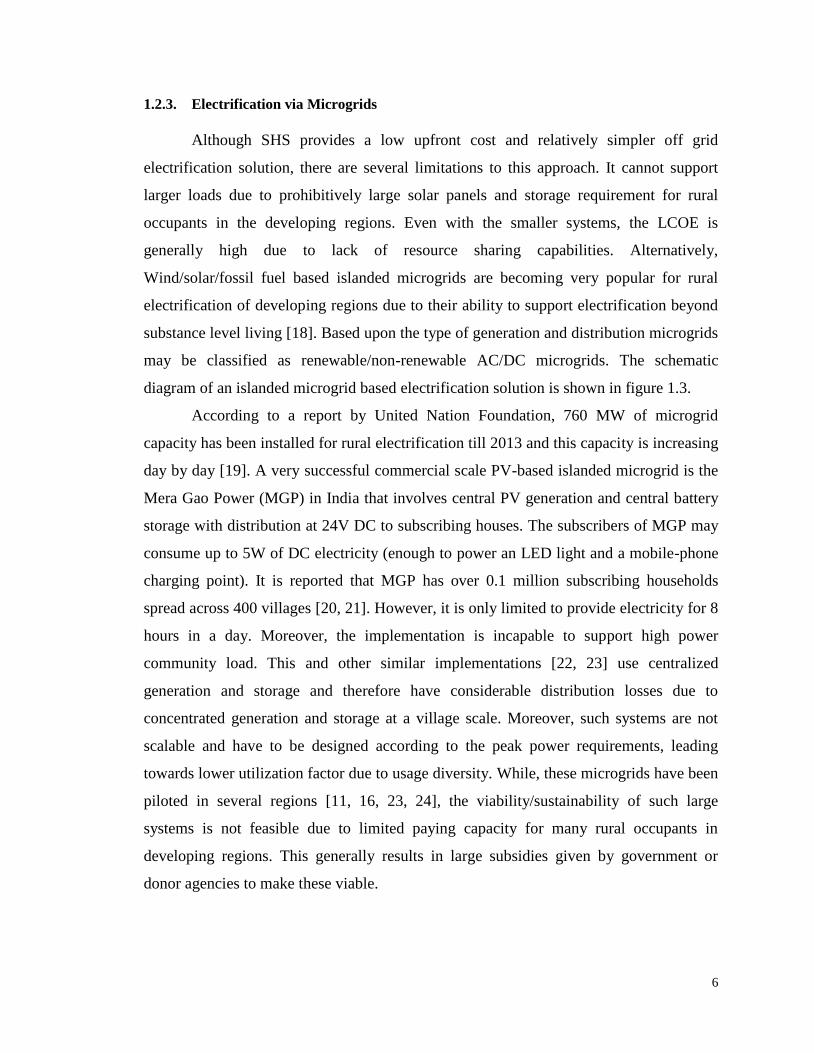
1.2.3. Electrification via Microgrids

Although SHS provides a low upfront cost and relatively simpler off grid

electrification solution, there are several limitations to this approach. It cannot support

larger loads due to prohibitively large solar panels and storage requirement for rural

occupants in the developing regions. Even with the smaller systems, the LCOE is

generally high due to lack of resource sharing capabilities. Alternatively,

Wind/solar/fossil fuel based islanded microgrids are becoming very popular for rural

electrification of developing regions due to their ability to support electrification beyond

substance level living [18]. Based upon the type of generation and distribution microgrids

may be classified as renewable/non-renewable AC/DC microgrids. The schematic

diagram of an islanded microgrid based electrification solution is shown in figure 1.3.

According to a report by United Nation Foundation, 760 MW of microgrid

capacity has been installed for rural electrification till 2013 and this capacity is increasing

day by day [19]. A very successful commercial scale PV-based islanded microgrid is the

Mera Gao Power (MGP) in India that involves central PV generation and central battery

storage with distribution at 24V DC to subscribing houses. The subscribers of MGP may

consume up to 5W of DC electricity (enough to power an LED light and a mobile-phone

charging point). It is reported that MGP has over 0.1 million subscribing households

spread across 400 villages [20, 21]. However, it is only limited to provide electricity for 8

hours in a day. Moreover, the implementation is incapable to support high power

community load. This and other similar implementations [22, 23] use centralized

generation and storage and therefore have considerable distribution losses due to

concentrated generation and storage at a village scale. Moreover, such systems are not

scalable and have to be designed according to the peak power requirements, leading

towards lower utilization factor due to usage diversity. While, these microgrids have been

piloted in several regions [11, 16, 23, 24], the viability/sustainability of such large

systems is not feasible due to limited paying capacity for many rural occupants in

developing regions. This generally results in large subsidies given by government or

donor agencies to make these viable.

7

Figure 1.3 Schematic Diagram for Islanded Microgrid based Electrification

These limitations of conventional microgrid based electrification schemes can be

substantially overcome by the optimal selection of microgrid architecture and generation

technology.

1.3. Need for Viable Microgrid Architectures for Rural Electrification

Although the conventional schemes for rural electrification are being largely

deployed as a stop gap measure for energy poverty eradication, however, owing to their

limited potential, such schemes are not sufficient for wide scale deployment to achieve

the global objectives of SDG-7. With the growing population and associated

electrification requirements, there is the need of a robust, technologically advanced,

economically feasible, financially viable and widely adoptable electrification solution

that can grow in a bottom-up manner and support micro-financing for enhanced rates of

electrification. In order to advance towards more efficient topologies for RE, it is

important to review the recent technological advancements in microgrids which will lead

towards a more suitable candidate for future rural electrification deployments. Two major

aspects i.e. a) generation technology (renewable or non-renewable), b) type of

distribution (AC or DC) are critical in this regard and discussed in the sub-sections

below. Another critical factor is the architecture of DC microgrid with regards to

generation and storage resources placement. Concentrated placement of resources in

existing deployments generally limits the electrification capabilities from distribution loss

and scalability prospective and is discussed further in the next chapter.

Centralized Renewable/non-renewable Generation, Battery Storage and Charge Controller Electrified Village

8

1.3.1. Suitable Generation Technology for Microgrid based Rural Electrification

A microgrid can be either AC or DC and is considered as a highly reliable

medium of generation and distribution of electrical energy by connecting distributed

generation (DG) units and critical loads in close proximity [25-30]. Microgrids may have

various renewable and non-renewable sources such as fuel cells, photovoltaic systems,

small diesel generators, wind turbines, and micro-turbines [25, 30-32]. Conventional

resources of generation including fossil fuel based generation in particular diesel based

generation systems result in carbon emission and are not considered as an attractive

solution for electrification due to their adverse effects on environment. Moreover, the

levelized cost of electricity and operation cost for such diesel based electricity generation

systems are higher and unviable for low-income communities.

Over last two decades, the renewable and alternate energy technologies has

gained world-wide interest as an effective alternative to reduce the dependence on fossil

fuels and to avoid their adverse effects on climate change [33, 34]. Therefore, renewable

energy resources, in particular wind and solar energy generation are being largely

adopted by microgrid practitioners due to their green and environment friendly nature

[35-37]. Among all other renewable technologies, installations based upon solar energy

extraction using Photovoltaic (PV) systems are more successful due to natural availability

of sunlight, relatively simpler schemes of installation, environment-friendly nature and

noise-free operation [38, 39]. The consistent reduction in PV panel prices, Feed-in-Tarrifs

(FiT) and favorable governmental policies to incorporate renewable energy resources

have also encouraged domestic consumer to invest in this technology to contribute

towards sustainable electricity generation. Therefore, due to green nature, abundant

availability of solar energy in most of the non-electrified areas (above 5.5 kWhr/m2/day

for most of the regions) [14, 15], and constantly diminishing panel prices, solar PV

microgrids are highly suitable for remote areas electrification [24]. Also, battery

technology has become mature and allowing deeper discharges and longer life at a

lowering cost [40], therefore, PV/battery based microgrids can be considered as optimal

choice for future electrification projects.

9

1.3.2. Suitable Mode of Distribution and Utilization for Microgrid Based Rural

Electrification

Depending upon the mode of generation, distribution and utilization, microgrids

may be classified either as AC microgrids or DC microgrids. Several researches between

the comparison of AC and DC microgrids has been presented in literature [41-43]. Due to

their inherent simplicity, higher power quality, enhanced efficiency and straight forward

controllability, DC microgrids are preferred over AC microgrids for rural electrification

applications [41-47]. A detailed tabular comparison between the design, implementation

and operational characteristics of AC and DC microgrid is shown in Table 1.

Solar photovoltaic (PV) produces DC, batteries store DC and most modern loads

are now DC, which allows local power generation and distribution through DC

microgrids with source closely matching the load profile. Compared to traditional AC

distribution, DC microgrids are significantly more efficient due to no DC-AC or AC-DC

conversion when implemented with distributed generation (DG). These systems have

end-to-end efficiency of around 80% (for DC loads) compared to AC microgrids which

are less than 60% efficient [42, 48]. Along with higher efficiency, DC microgrids and

associated distribution has the inherent advantage of less conductor usage for distributing

the same amount of peak power in comparison to AC distribution. Therefore, cost

associated with distribution conductors can be substantially reduced using DC

distribution [49]. Also, DC distribution is more resilient from power quality issues and its

reliability is relatively higher in comparison to AC distribution [50]. These all factors

make PV/Battery based DC microgrids as an optimal choice for rural electrification

applications.

PV/battery based DC microgrids can be further optimized from architecture

prospective and this is further highlighted in next chapter.

10

Table 1. 1 Detailed Comparisons between AC and DC Microgrids

Factors Sub Factors DC Microgrid AC Microgrid

Energy

Efficiency

Distribution losses Lower [41, 51] Higher [41, 51]

Conversion losses Lower due to inherent DC

nature of the loads [52, 53]

Higher due to AC/DC

conversions [52, 53]

Overall Efficiency 85-77% for DC loads,

<63% for AC loads [54].

< 60% with DC

generation [54].

Conductor

Usage

Power carrying capability

Higher for the same

conductor thickness [49].

Lower for the same

conductor thickness [49].

Cu mass usage 33% higher than AC [49]. 33% lower than DC [49].

Cost

Conductor cost Lower [49]. Higher [49].

Protection cost Higher due to electronic

relays [55].

Lower due to mechanical

switches/ relays [55, 56].

Protection Response time Higher [56]. Lower [56].

Cost Higher due to non-

availability of zero crossing

Lower due to zero

crossing availability [57].

Reliability

Critical load handling

capability

Higher (data centres and

UPS systems ) [50].

Lower [50].

Pulsed load handling

capability

Higher [47, 58]. Lower [47, 58].

generator synchronization Simple [59-61]. Complex [59-61].

Power

Quality

Transient stability Higher [47, 61]. Lower [47, 61].

Power quality to loads Better [42, 61]. Lower [42, 61].

Data

Analysis and

computation

Planning, operation and

Control studies

Simple due to involvement

of real numbers [42].

Complex due to

imaginary numbers [42].

11

2 Architecture of Solar PV based DC

Microgrid

As discussed in chapter 1, solar PV based microgrids provide an efficient and

potentially cost-effective rural electrification solution; however, there are several issues

which must be addressed for their widespread deployments. The limited electrification

capabilities of existing PV based DC microgrid architectures in terms of their low

distribution efficiency, inability to handle large power communal loads, non-modularity

in their structure and limited scalability are elaborated in this chapter. Based upon the

highlighted limitations, a scalable DC microgrid architecture having inherent advantages

of higher efficiency, modular scalability, simplified communication-less control and

efficient aggregation of power for larger household or communal loads is detailed for

future electrification implementations.

2.1. Central Generation Central Storage Architecture

Figure 2.1 shows the topological diagram of a typical centralized DC microgrid

architecture used for many rural electrification implementations. Such an architecture in

which generation (PV panels) and storage (batteries) are placed on a central location is

referred as central generation central storage architecture (CGCSA). CGCSA has a

unidirectional flow of power from a central location with solar PV generation and storage

to households. The load for community center consisting of school computing or health

care unit may also be powered from the central distribution line, however, generation

capacity has to be designed as per over all peak load requirements. A single DC-DC boost

converter is required for maximum power point tracking (MPPT) of PV panels and

stepping up the voltage to microgrid distribution voltage level. At the consumer end

another DC-DC converter is required to step down the microgrid voltage level to

household devices level.

12

Figure 2. 1 Central Generation Central Storage Architecture (CGCSA) of PV based DC Microgrid

Prominent practical implementations for rural electrification through CGCSA of

PV/battery based DC microgrids include micro-solar plants in Chhattisgarh, by

Chhattisgarh renewable energy development agency (CREDA) in India [22, 23].

CREDA has deployed 576 PV based DC microgrids with cumulative capacity of

2.15MW, serving around 31000 customers in remote areas [19]. MGP discussed in the

previous chapter, subscribed by 0.1 million consumers, is also based upon CGCSA [20,

23]. Similarly, in 2012, Uttar Pradesh and Renewable Energy Development Agency

(UPNEDA), installed 1 kW DC microgrids in 11 districts covering around 4,000 houses

[62]. The Jabula project in Cape Town, South Africa is another successful model, where

Zonke Energy installed a PV/battery based DC micro-grid (750WP) to serves nine

families residing in informal settings with basic electricity [58].

In all the above mentioned practical deployments, centralized architecture of

PV/battery based DC microgrid is being used. This energy is then delivered to

subscribing households via distribution conductors and therefore, distribution losses are

associated with the delivery of energy. The distribution losses in this architecture depend

upon the distribution voltage level and size of mass produced conductor used for

distribution. Generally, line losses reduce at higher distribution voltages and the wider

PV

PanelsDC- DC Converter

Battery

StorageDC- DC Converter

House 1

LoadDC-DC

Converter

House 2

LoadDC-DC

Converter

House n

LoadDC-DC

Converter

Communal

LoadDC-DC

Converter

DC- DC

Converter

Central Generation Central Storage Point

13

area conductor size, while the system exhibit lower efficiency and higher line losses at

lower distribution voltage and lower conductor area used for distribution. The central

positioning of the resources is generally beneficial from the perspective of control, where

overall generation and storage level (state of charge) are reliably monitored. However,

this results in higher distribution losses and rigidity in terms of future expansions [15].

Moreover, powering a high power communal load will substantially enhance the

distribution losses in the path of power flow.

Another draw-back associated with CGCSA is that its generation and storage

capacity has to be designed as per peak power requirements of the load, thereby

increasing the upfront capital cost of installation. In such a topology, the advantage of

usage diversity cannot be extracted. For instance power provisioning to high power

communal loads including water filtration plant, computing load of a school or load of

medical equipment in a health care unit results in a substantial increase in the required

capacity and associated cost of the installation. Moreover, at the day time, when there is

enough production by the PV panels and lighting load requirement at houses is

comparatively negligible, the excessive power generated by the PV panels cannot be

utilized optimally after the storage system has fully charged. Thereby, excessive power

will be wasted within panels making the overall scheme essentially sub-optimal in terms

of resource utilization.

Considering the example of ―Mera Gao Power‖ (MGP) in India, which provides

only 5 W of DC power to each subscribing house, with a limit of 0.2 amps—enough to

power two LED lights and a mobile phone-charging point [20, 23]. Although ‗small

power‘ is beautiful, it is unable to drive high power community loads [63]. Due to very

limited power supply, such a scheme is unlikely to alleviate poverty in rural areas or

contribute to significant improvements in their socio-economic circumstances [16]. If

such a central generation central storage architecture (CGCSA) is implemented for high

power loads for households (50 W or higher), the losses associated with the distribution

of energy are significantly higher, thereby making the scheme unviable. The framework

for detailed loss analysis based upon Newton – Raphson method modified for DC power

flow will be presented in the Chapter 3.

14

2.2. Central Generation Distributed Storage Architecture

Madduri et al. [54, 64] presented a central generation distributed storage

architecture for rural electrification. It has been shown that by distributing the storage

system at individual consumer nodes will result in reduced distribution losses, while the

distributed power may be intelligently stored or consumed at the load end using

household power management units (PMU). The provision of energy storage at local

houses results in higher efficiency compared to CGCSA, but this architecture is still

suboptimal in two respects: a) central PV generation requires a higher upfront cost

because a large nameplate capacity is required for the solar panel at the outset, resulting

in a cost barrier; and b) distribution to distant houses causes significant system losses.

Moreover, the presented architecture uses central PV generation and is unable to pool for

communal loads effectively without resource sharing capability. Therefore, architecture

with minimum possible distribution losses capable to integrate its resources in a scalable

manner is required to have an optimal solution for impactful rural electrification.

2.3. Other Distributed Architectures of DC Microgrid in Literature

Another PV based ad-hoc partially distributed DC microgrid architecture for rural

electrification proposed by Wardah et al. [65] integrates the power needed for several

consumers (up to 20) into a single generator unit. However, the overall distribution is at

48 V, which renders it impractical for the requirements of larger households or a

community level load due to higher distribution losses. Moreover, in this architecture,

peer to peer electricity sharing was enabled by GSM based communication between

power management units (PMU) of generating modules (houses having PV generation,

battery storage and local load) and consuming modules (houses having only local loads

without any generation or storage facilities). The advantages of distributed architecture

are mainly reduction in distribution losses and modularity in structure. However,

coordination among the distributed resources and control for power sharing becomes

extremely challenging. Several strategies for hierarchical and supervisory and droop

control of DC microgrids have been proposed in [8, 66-70]. However, these require an

extra layer of monitoring, sensing and communication, which in turn enhances the cost

and complexity of the system. For rural electrification purposes, such a complex, high

15

cost and communication based distributed architectures is not preferable due to

constraints of limited funding.

What is needed instead is an architecture that can scale in power for individual

homes and also support large (kilowatt level) loads, such as water pumps and

refrigeration units, for communal use. The architecture should be scalable and built

through bottom-up approach so that it can enable micro-financing for successful business

model as well as wide adaptability. The architecture must have (a) resource sharing

capability and (b) potential of higher powers even with limited roof-top PV production

and (c) ability to fulfill the community load demands. Such systems can in principle work

as a primary grid or in parallel with the surrounding AC grid. In this thesis, one such PV

based DC microgrid system is proposed that allows a scalable approach with minimal

upfront investment to run the electricity needs along with the provision of higher powers

for a communal load.

Therefore, for rural electrification purposes, architecture having low cost

deployment lower distribution and conversion losses, higher end to end efficiency, high

reliability, scalability along with modularity in structure, resource sharing feature and

capability to drive high power communal load is highly desirable. Architecture with these

characteristics is a true rural electrification architecture that can provide beyond

subsistence level power provisioning and can genuinely contribute towards the socio-

economic uplift of the society and an architecture with these characteristics can

substantially enhance the electrification rates to achieve the global objectives of SDG-7.

2.4. Proposed Distributed Generation Distributed Storage Architecture

In light of the limitations on (a) distribution efficiency, (b) power supply for

household-level loads, (c) provision of communal loads, (d) rigidity in future expansion,

and (e) requirements for extensive communication based control techniques in the above-

mentioned architectures for a DC microgrid, we propose a solar PV based scalable,

distributed generation and distributed storage architecture (DGDSA) with a novel

resource (power)-sharing provision among the distributed resources (see Fig. 2.2). The

architecture has the built-in advantages of (a) higher efficiency because of distributed

generation and distributed storage, (b) modular scalability for future expansion, (c)

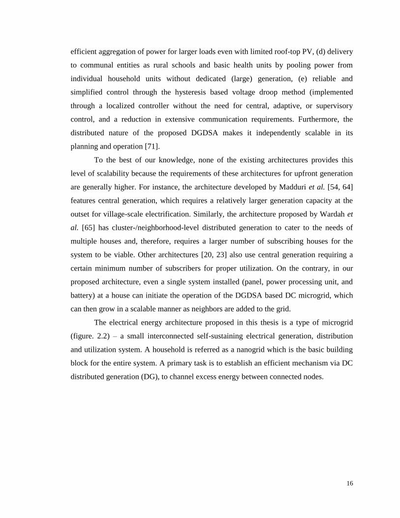
16

efficient aggregation of power for larger loads even with limited roof-top PV, (d) delivery

to communal entities as rural schools and basic health units by pooling power from

individual household units without dedicated (large) generation, (e) reliable and

simplified control through the hysteresis based voltage droop method (implemented

through a localized controller without the need for central, adaptive, or supervisory

control, and a reduction in extensive communication requirements. Furthermore, the

distributed nature of the proposed DGDSA makes it independently scalable in its

planning and operation [71].

To the best of our knowledge, none of the existing architectures provides this

level of scalability because the requirements of these architectures for upfront generation

are generally higher. For instance, the architecture developed by Madduri et al. [54, 64]

features central generation, which requires a relatively larger generation capacity at the

outset for village-scale electrification. Similarly, the architecture proposed by Wardah et

al. [65] has cluster-/neighborhood-level distributed generation to cater to the needs of

multiple houses and, therefore, requires a larger number of subscribing houses for the

system to be viable. Other architectures [20, 23] also use central generation requiring a

certain minimum number of subscribers for proper utilization. On the contrary, in our

proposed architecture, even a single system installed (panel, power processing unit, and

battery) at a house can initiate the operation of the DGDSA based DC microgrid, which

can then grow in a scalable manner as neighbors are added to the grid.

The electrical energy architecture proposed in this thesis is a type of microgrid

(figure. 2.2) – a small interconnected self-sustaining electrical generation, distribution

and utilization system. A household is referred as a nanogrid which is the basic building

block for the entire system. A primary task is to establish an efficient mechanism via DC

distributed generation (DG), to channel excess energy between connected nodes.

17

Figure 2. 2 Conceptual Diagram of Distributed Generation Distributed Storage Architecture

(DGDSA) of DC Microgrid with Contributing Nanogrids and Communal Load

For instance, in figure 2.2, PV panels at rooftop (home ‗a‘) should be able to

provide energy to a neighboring house (home ‗b‘) if the PV produced power is not being

utilized in home ‗a‘ and vice versa. Similarly, if both home ‗a‘, home ‗b‘ up to home ‗n‘

have surplus power then there must be a mechanism to allow this power to be utilized at

communal loads. Inherently, PV panels continuously provide power during the presence

of sunlight and if not utilized properly, this power is wasted within the panel. Therefore,

in a communal setting, the surplus DC power produced by all the panels must also be

utilized by communal loads such as water pumping for drinking/irrigation, medical

equipment in basic health units, lighting and computing loads in school etc. Such large

communal loads otherwise (standalone basis) are often very expensive and unsustainable

in rural scenarios of developing countries. Although solar energy is taken as the primary

source however other sources both renewable and non-renewable can be integrated at a

common coupling point. In addition, integration with utility grid could also be possible

allowing bidirectional flow of power. However, integration of utility AC grid or other

sources is out of scope for the current implementation as this work primarily focuses on

the implementation and operation of the microgrid itself in off-grid communities.

18

2.4.1. Model of Nanogrid

A nanogrid is a basic building block and integral part of DGDSA of microgrid

that integrates its resources in a scalable manner into the community. Each

house/nanogrid has its own generation in the form of a roof-mounted solar PV panel, its

own battery storage and a few DC loads. Therefore, each nanogrid has the capability to

work independently in islanded mode or in conjunction with the other nanogrids in the

architecture in power sharing mode. The bidirectional flow of power is controlled via

power electronic converters referred to as central power processing units (CPPUs). A

CPPU contains a microcontroller along with a maximum power point tracking (MPPT)

based DC-DC converter and a bidirectional flyback converter.

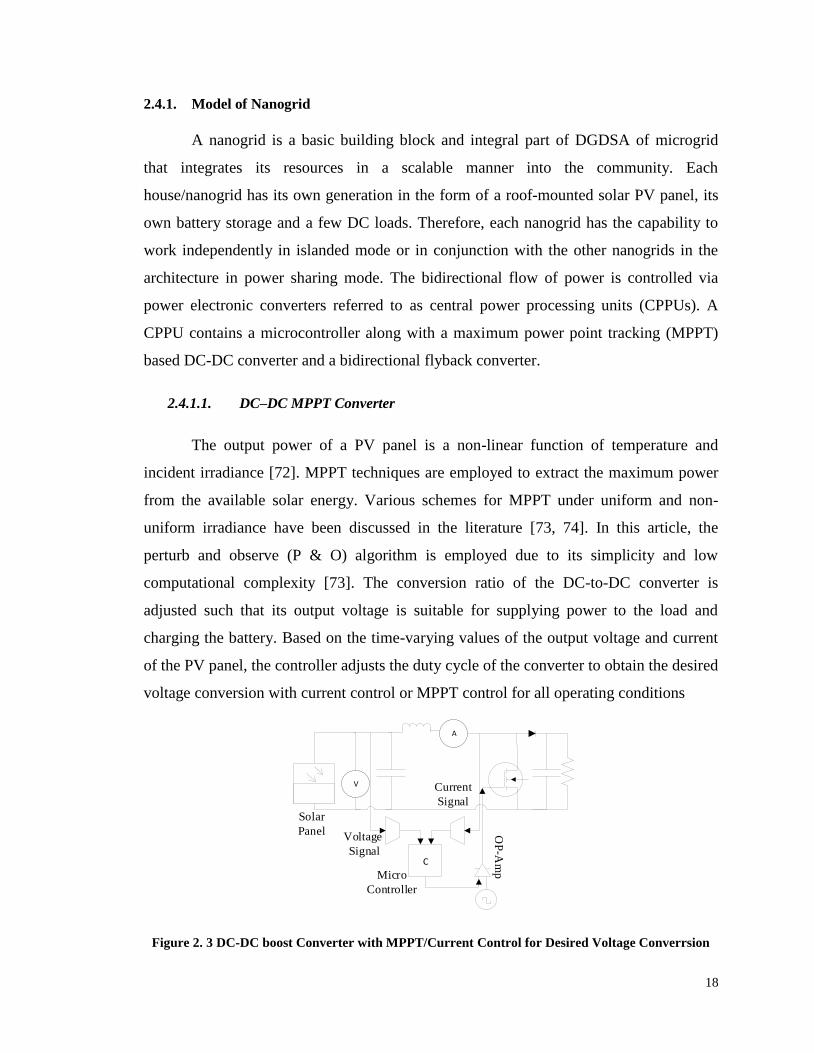
2.4.1.1. DC–DC MPPT Converter

The output power of a PV panel is a non-linear function of temperature and

incident irradiance [72]. MPPT techniques are employed to extract the maximum power

from the available solar energy. Various schemes for MPPT under uniform and non-

uniform irradiance have been discussed in the literature [73, 74]. In this article, the

perturb and observe (P & O) algorithm is employed due to its simplicity and low

computational complexity [73]. The conversion ratio of the DC-to-DC converter is

adjusted such that its output voltage is suitable for supplying power to the load and

charging the battery. Based on the time-varying values of the output voltage and current

of the PV panel, the controller adjusts the duty cycle of the converter to obtain the desired

voltage conversion with current control or MPPT control for all operating conditions

Figure 2. 3 DC-DC boost Converter with MPPT/Current Control for Desired Voltage Converrsion

V

A

Micro

Controller

Solar

PanelVoltage

Signal

Current

Signal

OP

-Am

p

C

19

The continuous conduction mode (CCM) governing equations of DC-DC boost

converter for the output voltage gain M(D), current ripple across the inductor ΔIL and

voltage ripple across the capacitor ΔVC are given by (2.1), (2.2) and (2.33) respectively

[75].

DV

VDM

out

in

1

1)( (2.1)

)( sDTL

VL

I in (2.2)

)(2

sDTRC

VcV out (2.3)

Where, Vin is the input voltage, Vout is the output voltage, Ts is the time period

based on switching frequency of the converter, L is the value of inductance to have the

desirable current ripple C is the value of output capacitor to have a desirable ripple in

output voltage and D is the duty cycle of the converter. The converter switches its mode

of operation when excess power is being generated and is not useable for battery charging

or neighborhood sharing. The switching of DC-DC boost converter between MPPT

control and current mode control based upon the external grid state and internal nanogrid

state (state of generation and storage) is discussed in details in Chapter 4.

2.4.1.2. Bidirectional Flyback Converter

A bidirectional flyback converter is employed to enable the resource sharing feature, as

it allows for the transfer of power from nanogrids to the microgrid, and vice versa. The

bidirectional power flow in the proposed flyback converter is attained through modified

switch realization, i.e. replacing the diode of conventional flyback converter with another

controlled mosfet switch. The switch position is also changed to ensure that the source is

grounded without affecting the continuity of the circuit. This allows optimum gate driver

circuit design without the requirement of complex bootstrapping circuit [76].

Flyback converter has inherent advantages of simple design and less component usage

over other types of buck-boost converters, therefore, highly suitable for DC microgrid

applications. Along with the higher conversion ratio, it also allows the use of inherent

magnetizing inductance Lm of the flyback transformer, thus mitigating the need of extra

20

inductor for converter energy transformation. Also, it provides isolation between multiple

nanogrids to ensure reliability in architecture, in case if fault occurs on the grid side or

nanogrid mosfet becomes short circuit. Bi-directional switch realization of flyback

converter is shown in figure. 2.4.

The continuous conduction mode (CCM) governing equations of flyback

converter for the output voltage gain Mf(D) and transformer DC component of

magnetizing current Im are given by (4) and (5)

D

Dn

V

VDM

out

inf

1)( (2.4)

'RD

nVIm (2.5)

Where, Vin is the input voltage, Vout is the output voltage, n is the turn ratio of

transformer and D is the duty cycle of the converter. Multi-mode adaptive control of

isolated bi-directional converter ensuring coordinated resource sharing among the

contributing naogrids is detailed in chapter 4.

Figure 2. 4 Modified Switch Realization of Flyback Converter enabling Bidirectional Power Flow

among the Contributing Nanogrids

V V

120

V D

C M

icro

grid

Transformer

Mosfet

Switches

12V

DC

Batte

ry

Voltage

Signal

OP-Amp

Micro

ControllerVoltage

Signal

21

2.4.2. Model of a Village and Microgrid Scheme of Interconnection

Depending upon the structure, a typical village containing n houses is divided into

x segments with n/x houses per segment, as shown in figures 2.5 and 2.6. Power is

supplied to the load in each household via a flyback converter that, along with the

resistance of the supplying wire, is modeled as a constant power bus and represented by a

distributor resistance. The interconnection resistance between two consecutive nanogrids

is modeled as feeder resistance.

Two interconnection schemes are considered and shown in figure 2.5 and 2.6. Fig.

2.5 shows the radial interconnection of nanogrids that lowers the cost of the conductor in

the system design. However uneven loading, non-uniform voltage distribution, high-

voltage dips at the rear end, and subsequent reliability issues render radial schemes a

relatively poor choice for the optimal distribution of power [77, 78]. Therefore, to address

these issues, the ring main scheme of interconnection is proposed (figure 2.6). It uses an

extra layer of conductors (dashed lines) to connect feeders at the periphery of radial

architecture in a ring main fashion. Thus, at the cost of extra conductors, higher

efficiency and increased reliability are achieved, even at comparatively low distribution

voltages.

Figure 2. 5 Proposed Architecture of the Radial Schemes of Interconnection with Elaborated Single-

Unit Design

x-1(n/x)

1 2 n/x (n/x)+1

Segment 4 Segment x

Segment 1 Segment 2

Segment 3

(n/x)+2 2(n/x)

2(n/x)+1 3(n/x)

3(n/x)+1 4(n/x) n

Battery/

PV Panel

Household

Load

Distributor

Feeder

Bus 1

Bus 2

Single Cell in a Segment

(Nanogrid)

22

Figure 2. 6 Proposed Architecture of the Ring Main Schemes of Interconnection

. Using the values of the feeder and the distributor resistances, based on the scheme

of the interconnection and topological configuration of a village, a conductance matrix G

can be calculated to model it. For a village with n houses, G is of the order of 2n × 2n, as

each house contains two buses: 1) a load bus at the interconnection of the distributor

resistance and the load bus, and 2) another bus at the interconnection of the feeder and

the distributor resistances (figures 2.5 and 2.6). Thus, elements of the conductance

matrices Gij and G can be written in terms of individual conductance gij between any

arbitrary buses i and j, where i may vary from 1 to 2n:

ji ;

i; 2

1

ij

ij

ij

g

jn

ij

j

g

G

(2.6)

nnRG

G

G

G

G

nnn

n

n

22;

G G

G G

G G

2,2 2n,21,2

2,222 21

2,11211

(2.7)

The conductance matrices developed here will be used for power flow analysis

modified for DC power flow in presented chapter 3 for the assessment of central and

distributed architectures of DC microgrids from voltage dips, distribution efficiency and

distribution losses prospective at various LVDC voltage levels and conductor sizes.

x-1(n/x)

1 2 n/x (n/x)+1

Segment 4 Segment x

Segment 1 Segment 2

Segment 3

(n/x)+2 2(n/x)

2(n/x)+1 3(n/x)

3(n/x)+1 4(n/x) n

23

3 Power Flow Analysis of Solar PV

based DC Microgrid

In order to ascertain distribution losses, distribution efficiency and voltage drop in

various power provisioning scenarios of PV based DC microgrid operation, Newton-

Raphson method has been modified for DC power flow analysis. Based upon the

presented method, a comparative analysis of CGCSA and DGDSA with and without

communal load has been performed. In case of CGCSA analysis, optimal placement of

central generation and storage point is discussed in details, while in case of DGDSA

various power sharing scenarios have been evaluated to ascertain the efficacy of proposed

architecture.

3.1. Newton-Raphson Method Modified for Power Flow Analysis of DC

Microgrid

Power flow analysis is conducted through Newton-Raphson method and its application

is modified for our DC microgrid [79]. This is essential to ascertain various critical

elements of the proposed system such as total line losses, efficiency and maximal voltage

drops [77]. These parameters are used as an indicator for the selection of optimal

distribution voltage for DC microgrid. Conventionally, iterative algorithms such as Gauss

Seidel method, Newton–Raphson method and Fast Decoupled method are being used for

the load flow analysis of AC systems [77, 80]. Conventional AC power flow algorithms

cannot be directly applied for DC systems and have to be modified [81]. For our design,

load flow analysis is performed through a modified Newton-Raphson method discussed

in this chapter [79, 82]. This reduces the computational complexity in comparison to

conventional AC load flow analysis which involves complex Jacobian matrix calculation

for the determination of reactive power and voltage angles.

For DC microgrid operation, the interconnections between multiple nodes are

modelled as a power network shown in figure 3.1. Consider the case where there total n

busses and bus i corresponds to each interconnection point between neighboring houses

Each ith

household bus is connected to jth

household bus through a connecting wire with

24

its resistance modelled as a lumped conductance gij. Where, i and j may vary from 1 to n.

gi1, gi2 and gin are the respective value of the conductance between bus i and j.

Using KVL, current in bus i, Ii may be calculated by (3.1) [79]

n

jjiji VGI

1

(3.1)

Where, Gij is the conductance matrix of the power system and is given in terms of

individual conductance gij between bus i and j as given by (3.2).

jifor

ifor 1

ijg

jn

jijg

ijG

(3.2)

Instantaneous power at ith

bus Pi can be calculated as

n

jijjiiii GVVIVP

1

(3.3)

Using Taylor series expansion while neglecting higher order terms yields (3.4)

knV

kV

nV

knP

V

knP

nV

kP

V

kP

knP

kP

:

2

....

2

:

2 ....

:

2

2

:

2 (3.4)

Figure 3. 1 Power Network for Newton-Raphson method modified for DC Power Flow Analysis

25

Where, ΔP is the difference in scheduled power Psch and calculated power Pi

using (3.4) for k iterations. Desired voltage level of LVDC on which power flow analysis

has to be performed, is taken as reference for slack bus. Initial estimate of voltages for

generator busses are slightly higher than reference voltage and for load busses these are

assumed slightly lower than reference voltage. Using (3.4), change in voltages ΔV and

corresponding bus voltage V for k iterations are found until the difference between

scheduled and calculated power becomes negligible. After convergence, bus voltage V is

used to calculate the power of slack bus using (3.3). By using the converged value of

voltage at each bus, associated line losses LLg, percentage line losses %LLg, voltage drops

VDg, percentage voltage dip %VDg, and efficiency η for the dc microgrid are calculated

as given by (3.5) – (3.9).

n

i

n

jijjjiiijg VVVVVVGLL

1 12

1

(3.5)

n

ii

g

g

P

LLLL

1

0

%100 %

(3.6)

gLL%100

(3.7)

minmax VVVDg

(3.8)

max

minmax %100*

V

VV%VDg

(3.9)

Where, Vmax and Vmin are the maximum and minimum values of voltage at any bus after

kth

iteration. The methodology for power flow analysis is valid for DC microgrids and

will be used for the calculation of distribution losses, distribution efficiency and voltage

drops for CGCSA and DGDSA for various mass produced conductor sizes and voltage

levels. Based upon the methodology presented here, various power provisioning

scenarios will be evaluated for DGDSA, while, for CGCSA, effect of placement of

central generation and storage resources at various possible locations in the voltage will

also be discussed in details. Therefore, the presented Newton Raphson method modified

26

for power flow analysis will serve as the basis for microgrid architecture classification

from the prospective of distribution losses.

3.2. Case Study Parameters and Simulation Results

Voltage level is one of the prime factors affecting the operation, control, performance,

protection and safety of the microgrid based distribution systems [83-85]. Feasibility

studies of viable voltage levels for low voltage DC distribution in commercial and

residential systems are presented in [85, 86]. Due to the available applications and

devices, 12V, 48V, 120V, 230V, 325V and 380V are considered as viable voltages for

low voltage direct current (LVDC) distribution, where 12V is the most common voltage

for market available lead-acid batteries and DC loads including LED‘s and DC fans, 48V

is generally used in telecommunication sector, 120V rms and 230V rms are used as

standard distribution voltage in many countries, 325 is equivalent to the capacitor filtered

rectified voltage produced in 220V rms AC systems and 380V is generally employed for

DC distribution [83-85, 87]. They may be further categorized as very low, medium and

high levels of LVDC distribution.

For a given amount of power to be distributed, higher voltages yield higher efficiency

and lower line losses. While, lower voltages result in better safety aspects and reliable

protection against short circuit faults. In case of coupling with the public grid, safety and

protection issues are of more prime importance. Therefore, an optimal selection of

voltage level ensures an acceptable balance between safety, reliability and efficiency. In

CGCSA, distribution losses for 12 and 48V are high for driving considerable amount of

load i.e. 40W for 40 houses and solution does not converge, therefore, for CGCSA, these

two voltage levels are not considered.

The proposed architecture has been modeled around a typical village in developing

world containing 40 houses. All the houses are interconnected to DC microgrid via

‗feeders‘ and ‗distributors‘, where, the distance between consecutive houses (feeder) and

the length of the internal wiring (distributor) was 20 m, consistent with the situation in

rural settlements in developing countries as described by Varshney et al. [88]. Each

house is capable of driving 40W of DC load including lighting, fan and charging loads.

The rated power provisioning is in accordance with the market availability of DC loads

27

with three to four lighting bulbs (~4W each), one DC fan (~14 W) and one to two mobile

charging unit (~4 W). Similarly, for the village under analysis a communal load of up to

500W is considered for water filtration plant/pump for drinking purposes. Different

distribution conductors with wire gauge areas of 0.2 mm2 (local market name 3.0-

0.029‖), 0.45 mm2 (local market name 7.0-0.029¬‖), 2.5 mm

2, 6 mm

2, and 7.5 mm

2 were

considered for analysis. Using (3.6) – (3.9), %LLg, %η and %VDg are calculated for the

following scenarios.

3.2.1. CGCSA without Communal load

The CGCSA of a PV based DC microgrid is shown in figure 2.1. For the analysis

in this section peak load scenario is considered, where every house is demanding 40W

power. The optimal placement for generation and storage units are found by running an

iterative loop for all possible generation busses. System efficiency against each bus

placement is recorded and bus with highest efficiency is selected. Figure 3.2 shows the

results for %VDg and %η for different voltage levels and different mass produced

conductors, when generation and storage units are placed at one of the starting or ending

points of the corner segments (Refer to figure 2.5).

Figure 3. 2 Typical % Voltage drop and Efficiency for CGCSA with Peak Load and Far End

Placement

0 1 2 3 4 5 6 7 8

75

80

85

90

95

100

Eff

icie

ncy

(%

)

Conductor Area (mm2)

400V

325V

230V

120V

28

Figure 3. 3 Typical % Voltage Drop and Efficiency for CGCSA with Peak Load and Central

Placement

From figure 3.2, it can be observed that at higher voltages, distribution efficiency

is higher while voltage drops are relatively lower, while thin conductors are not suitable

at low voltages, resulting in very high voltage drop. Voltage drop is a direct measure of

the converter requirements in the system; therefore, voltage drop generally higher than

20% is not suitable for reliable operation of the microgrid.

Figure 3.3 shows the results for %VDg and %η, for different voltage levels and

different mass produced conductors, when generation and storage units are placed at

center of segment 3 (Refer to figure 2.5) . From figure 3.3, it may be concluded that

higher efficiencies and lower voltage drops are achieved by placing generation and

storage unit at central location as compared to far end region placement.

3.2.2. CGCSA with Communal load

Figure 3.4 shows the results for %VDg and %η for communal load scenario, in

which each of the houses is restricted to 30W, while 400W is supplied to communal load.

This may be a typical scenario where during first half of a day, the power is allocated for

computing school for children with limited power delivered to households. The optimal

location for communal load on the microgird is found by running an iterative loop for

placement at all possible load busses and comparing system efficiency. The bus with

highest efficiency is selected which in our proposed case of CGCSA is located at the

center point of the central segment (see figure 2.5).

0 1 2 3 4 5 6 7 8

76

80

84

88

92

96

100

Eff

icie

ncy

(%

)


400V

325V

230V

120V

29

Figure 3. 4 % Voltage drop and Efficiency for CGCSA with Communal Load and Central Placement

3.2.3. DGDSA with Radial Scheme of Interconnection

The DGDSA of a PV based DC microgrid is shown in figure 3.5. Typical and

peak load scenarios are evaluated for DGDSA with radial scheme of interconnection. In

typical load scenario, the power sharing between houses and grid is taken as ±20% (a

house can demand 20% more or supply 20% of its rated power). Power sharing is

randomly scheduled at various household between ±8 W i.e. 20% of rated power, therefor

power losses and voltage drops are very limited. Results for percentage voltage drop and

efficiency (figure 3.5) show that with moderate size conductor such as 2.5 mm2 the loss is

low for 120V and higher voltages with efficiencies above 99%.

The situation changes significantly when power flow provision is kept higher to a

household. Under this peak load scenario, a house can consume twice of its rated power

and it can supply all available power to the grid. In this scenario, power is randomly

scheduled either +40W or -40W at each household bus. Results show that efficiency is

lower for low voltages and a significantly higher cost of thick conductor must be incurred

for this topology to achieve lower line losses as shown in figure 3.6.

0 1 2 3 4 5 6 7 8

75

80

85

90

95

100

Eff

icie

ncy

(%

)


400V

325V

230V

120V

30

Figure 3. 5 Percentage Voltage Drop and Efficiency at Different Voltages and Different Conductor

Sizes for Typical Load sharing with Radial Scheme of Interconnection (Common Load Sharing

Radial DC Microgrid)


Sizes for Peak Load sharing with Radial Scheme of Interconnection (Peak Load Sharing Radial DC

Microgrid)

3.2.4. DGDSA with Ring-Main Scheme of Interconnection

In order to mitigate issues with Radial DGDSA, we proposed a more efficient and

reliable ring-main topology (refer to figure 2.5). This topology significantly improves the

efficiencies at peak load sharing in comparison to radial topology at the cost of extra

conductors in ring main topology which is used to connect the end nodes as shown in

figure 2.6.

0 1 2 3 4 5 6 7 898.4

98.6

98.8

99.0

99.2

99.4

99.6

99.8

100.0

Eff

icic

en

cy

(%

)


48V

120V

240V

325V

400V

0 1 2 3 4 5 6 7 8

50

60

70

80

90

100E

ffic

ice

nc

y (

%)


48V

120V

240V

325V

400V

31


Sizes for Peak Load sharing with Ring-Main Scheme of Interconnection. (Peak Load Sharing Ring-

Main DC Microgrid)

Ring-main interconnection topology also provides necessary redundancy to

ensure service operation in grid disconnection due to a fault or broken wires. The results

for peak load sharing for ring-main scheme have been shown in figure 3.3-3.7. From the

comparison of figures 3.6 and 3.7, it is evident that ring-main topology has higher

efficiency and less voltage drops in comparison to radial scheme of interconnection. For

instance, in case of peak load sharing at 120V and 2.5mm2 conductor size, ring-main

scheme exhibits higher efficiency (95.18%) as compared to radial scheme (92.66%).

Similarly, maximal voltage drops which are a direct measure of converter requirements,

are lower for ring-main scheme of interconnection in comparison to radial scheme for all

voltage levels and conductor sizes under considerations. The tabular comparison between

radial and ring-main DGDSA power flow will be presented in the subsequent sections.

3.2.5. DGDSA with Communal Load and Ring-Main Scheme of Interconnection

In order to analyze the performance of DGDSA under communal load scenario, with

ring-main scheme of interconnection among the contributing nanogrids, the power

scheduling has been adjusted such that each and every household/ nanogrid contribute

10W for communal load. Therefore, an aggregation of resultant power drives a

communal load of 400W.

0 1 2 3 4 5 6 7 850

60

70

80

90

100

Eff

icie

nc

y (

%)


48V

120V

240V

325V

400V

32

Figure 3. 8 Percentage Line Losses and Efficiency at Different Voltages and Different Conductor

Sizes for Communal Load Case with Ring-Main Scheme of Interconnection

This is the main advantage of such a nanogrid based scheme that dedicated power

resources need not be planned/installed for driving communal loads, including the

pumping load for water filtration plant or irrigation system, computing load of a school or

medical equipment load of a hospital. At day time when enough sunlight is available and

each household is producing more than its local requirements, power may be pooled up

for community load purposes. The power electronic interface and associated control

schemes for this coordinated power sharing is discussed in details in chapter 4. The

analysis performed using Newton – Raphson method modified for DC power flow

showed that for the selected parameters, the distribution losses were less than 3% even at

a communal load of 400 W as shown in figure 3.8. Also voltage drops are within limited

range of ±15 % even at lower voltage levels of LVDC i.e. 48V and 120V.

3.3. Summary of Power Flow Comparison between CGCSA and DGDSA

Due to distributed placement of resources in DGDSA, distribution losses

associated with the delivery of power are relatively lower. In those scenarios, when each

household is relying on its local resources without any exchange from the neighboring

households, distribution losses are negligible. Even, in the case of typical power sharing

among households, distribution efficiency is above 98% for all voltage levels and

conductor sizes.

0 1 2 3 4 5 6 7 8

60

70

80

90

100

Eff

icie

ncy (

%)


48V

120V

240V

325V

400V

33

In worst possible scenarios, when all the households are exchanging their rated

power, distribution losses are still less than the case of CGCSA. Therefore, due to its

inherent distribution of resources near to local load, DGDSA has better distribution

efficiency in comparison to CGCSA of DC microgrid for all of its operation modes. In

order to make a comparison between both the architectures, they are compared on the

same level of system loading. A typical conductor mass of 2.5 mm2 cross section is

selected.

Table 3.1 show the comparison between the system parameters (Percentage line

loss, Percentage voltage drop and efficiency) of CGCSA and DGDSA for communal load

scenario, where 400W power is supplied to communal load. From the results summarized

in table 3.1, it may be concluded that for uniform system loading conditions, DGDSA has

comparatively higher efficiencies, lower line losses and lower voltage drops in

comparison to CGCSA due to distribution of resources, usage diversity and mutual

resource sharing capabilities.

Table 3. 1 Communal Load Comparison between CGCSA and DGDSA

Voltage

Level

(V)

Cond.

Area

(mm2)

CGCSA

DGDSA

LLg (%) VDg

(%)

η

(%)

LLg

(%)

VDg

(%)

η

(%)

120 2.5 8.11 8.86 91.89 3.30 3.52 96.70

230 2.5 2.38 2.53 97.62 0.80 0.84 99.20

325 2.5 1.33 1.43 98.67 0.44 0.45 99.56

400 2.5 0.89 0.96 99.11 0.29 0.30 99.71

34

3.4. Power Flow Comparison between Radial and Ring - Main scheme of

interconnection for DGDSA of Microgrid

As evident from results, DGDSA has superior characteristics in terms of higher

distribution efficiency, lower distribution losses and lower worst voltage drops in

comparison to CGCSA. Further, at the cost of extra conductor, distribution losses and

worst voltage can further be reduced and system reliability can be increased at the same

time using ring- main scheme of interconnection. Therefore, a comparison between radial

and ring-main scheme has been illustrated to develop the superiority of ring-main scheme

over radial scheme for the same level of system loading and parametric conditions. For

the purpose of comparative analysis following cases are considered.

3.4.1. Typical Load Comparison between Radial and Ring- Main Scheme of DGDSA

Table 3.2 illustrates the comparative results of system parameters (Percentage line

loss, Percentage voltage drop and efficiency) for typical case of power sharing, in which

each house is either supplying or demanding 20% of its rated power, at conductor size of

2.5 mm2. From tabular comparison (Table 3.2), it is evident that ring-main scheme is far

more superior in terms of higher efficiency, lower distribution losses and lower voltage

drops in comparison to radial scheme.

Table 3. 2 Typical Load Comparison between Radial and Ring-Main DC Microgrid

Voltage

(V)

Area

(mm2)

Radial Microgrid

Ring-Main

Microgrid

LLg

(%)

VDg

(%)

η

(%)

LLg

(%)

VDg

(%)

η

(%)

48 2.5 0.79 1.89 99.21 0.58 1.04 99.42

120 2.5 0.13 0.30 99.82 0.09 0.17 99.91

400 2.5 0.02 0.03 99.95 0.02 0.01 99.99

35

3.4.2. Peak Load Comparison between Radial and Ring- Main Scheme of DGDSA

Table 3.3 illustrates the comparative results of system parameters (Percentage line

loss, Percentage voltage drop and efficiency) for the case of peak power sharing, in which

each house is either supplying or demanding 100% of its rated power, at conductor size

of 2.5 mm2. From tabular comparison (Table 3.2), it is evident from table that ring-main

scheme is far more superior in terms of higher efficiency, lower distribution losses and

lower voltage drops in comparison to radial scheme. Even at very low voltage level of

LVDC i.e. 48V, distribution efficiency is above 82% at peak power sharing, in

comparison to radial scheme where distribution efficiency is 76% only (6 % gain in

efficiency at the cost of extra conductor). Since lower voltages of LVDC i.e. 48V and

120V are considered safe for indirect touch and requires less protection in comparison to

higher voltage levels, i.e. 230V, 320V and 380V, therefore, with the ring-main scheme of

interconnection, lower voltages can be used for distribution without significant reduction

in the distribution efficiency. Therefore, ring-main scheme provides ensure reliability

along with higher distribution efficiency with minimum converter requirements to keep

the voltage dips minimum at the rare end of the microgrid.

Table 3. 3 Peak Load Comparison between Radial and Ring-Main DC Microgrid

Voltage

(V)

Area

(mm2)

Radial Microgrid

Ring-Main

Microgrid

LLg

(%)

VDg

(%)

η

(%)

LLg

(%)

VDg

(%)

η

(%)

48 2.5 23.5 34.4 76.41 17.9 27.1 82.1

120 2.5 7.34 10.9 92.66 4.82 7.38 95.18

400 2.5 0.83 1.23 99.17 0.51 0.77 99.49

36

3.5. Hardware Setup, Parameters and Results for Power flow Analysis of DC

Microgrid

Scaled model of the microgrid is implemented as shown in figure 3.9. The

proposed model that originally includes 40 houses is scaled down to four houses, where

each house may either generate or consume the requisite amount of power under various

scenarios. The generation capacity of each house was implemented via power supplies

(ESCORT EPS3030T) and consumption capability through DC load banks (LABTECH

LEMSPL) available in the laboratory.

In case of DGDSA as show in figure 3.9, two houses are producing net power,

while remaining two houses are consuming net power. Similar arrangement is made for

CGCSA, where only one house generates net power and rest of three houses will

consume power. Peak load operation for DGDSA and CGCSA is evaluated and measured

results are found in agreement with the simulated results. The measured v/s simulated

results of percentage voltage drops for CGCSA and DGDSA for scaled down version are

shown in figure 3.10. Difference between simulated and measured results accounts for

the excessive resistive losses at the joints and terminal points.

Figure 3. 9 Hardware Implementation of Scaled down version for Power Flow Analysis

37

Figure 3. 10 Measured v/s Simulated %Voltage Drops Results at 120V, 230V, 325V and 400V for

a) DGDSA and b) CGCSA

Both radial DGDSA and ring-main DGDSA interconnection schemes are tested at

the specified voltage levels with appropriate conductor size of 2.5mm2 and results are

compared with simulation outcomes as shown in figure 3.11. Simulated and measured

line losses are normalized with respect to highest value of the losses in corresponding

scheme. Results show that there is a difference between simulated and hardware results.

Difference between simulated and measured results accounts for the excessive resistive

losses at the joints and terminal points in hardware setup. Moreover, it may be verified

from the results that the losses (both simulated and measured) in radial scheme of

interconnection are higher than ring-main scheme at all the specified voltage levels.

Figure 3. 11 Simulated v/s Measured Results for Normalized Line Losses in DGDSA with Radial and

Ring-Main Schemes of Interconnection

100 150 200 250 300 350 4000.00

0.02

0.04

0.06

Vo

lta

ge

Dro

p (

%)

Voltage (V)

Simulated Results

Measured Results

100 150 200 250 300 350 4000.00

0.05

0.10

0.15

0.20

Vo

ltag

e D

rop

(%

)

Voltage (V)

Simulateded Results

Measured Results

48 120 230 325 4000.0

0.2

0.4

0.6

0.8

1.0

No

rma

lize

d L

ine

Lo

sse

s

Voltage Levels (V)

Radial Scheme

Measured

Simulated

48 120 230 325 400

0.0

0.2

0.4

0.6

0.8

1.0

Norm

aliz

ed L

ine L

osses

Voltage Levels (V)

Ring Main Scheme

Measured

Simulated

38

3.6. General Conclusions Drawn from Power Flow Analysis of DC Microgrids

It is clear from figure. 3.2 to figure 3.11 that at higher voltages, line losses are less

while efficiencies are higher. For a kW range power to be distributed, higher voltages

yield higher efficiency and lower line losses. While, lower voltages result in better safety

aspects and reliable protection against short circuit faults. Safety is a critical concern and

at higher voltage levels, the system requires sophisticated and expensive protection

equipment. This limits our choice of voltage level depending on the amount of resources

available for the DC-Grid. It should be noted that DC breakers are more sophisticated and

cumbersome to manage in case of short-circuits or unwanted transients which may

require disconnection of the DC grid from nanogrids. For instance, in disconnection, the

arching is largely limited in AC due to zero crossing of the 50Hz frequency unlike a DC

grid. In DC systems the arcs may be higher and could potentially be hazardous.

In general lower voltages i.e. 24V and 48V do not have additional safety

concerns. The possibility of over current and associated over-heating hazards exist in

case of short circuits and such short circuits may be avoided using fuse protection after

the DC power source. For a practical system this must be added as an additional level of

safety. According to IEC 60950-1, voltage levels lower than 60V DC are considered safe

for direct touch and potentially do not create any electric shock hazard. Similarly,

according to NEC standards (NFPA 70), DC power sources having voltage levels lower

than 60V DC and maximum power capability of 100VA are referred as class 2 DC power

sources and are capable to eliminate electric shock hazards as well as fire protection

hazards. Emerge Alliance; an organization working on DC standards for buildings has

also nominated 24V DC as safe voltage against electrical shock/fire hazard with the

source capability to provide current less than 4.1A [89-91]. Therefore, in general, from

safety point of view 24V and 48V are relatively more safe levels of LVDC in comparison

to 120V 230V and 380V DC. However, voltage levels lower than 48V are not suitable for

distribution as voltage drop is much higher than 15%. Therefore, from system safety

point of view 48V distribution with a reasonable conductor can be considered as a choice

for future practical installations of DGDSA.

39

Moreover, as we move from 48V to higher voltage levels, losses are reduced and

efficiency is increased but this particular trend is not uniform as listed in Table 3.3 to

Table 3.3. As we move from 48 V to 120 V, there is a significant reduction in losses and

increase in the efficiency. The associated protection and safety requirements are not

excessive [92, 93]. Moving from 120V to 400V, percentage reduction in losses is not

significant for a typical conductor gauge of 2.5 mm2. However, system complexity,

protection and safety requirements increase significantly. Also, the distributed storage

and generation allows small current to flow on the grid and the arc lengths and arc energy

could be easily manageable even with 120V DC, in comparison to 240V AC [93].

Moreover, voltages lower than 120V are considered safe for indirect touch and require no

extra grounding and protective conductors [92]. While distribution at 120V is generally

less efficient than 400V, our proposed ring main interconnection between feeders and

microgrid allows minimal and loss adds necessary redundancy for a reliable but efficient

solution. 120V can therefore be considered as another optimal medium level voltage that

provides the desired trade-off between the safety aspects and efficiency, while keeping

voltage drops and line losses within acceptable range. For this particular village and

household load settings, selecting 120V voltage level will result in safer overall system

without a significant loss in the system efficiency. Therefore, for the considered

specifications of the village, 120 V using a conductor of area 2.5 mm2 and the ring main

scheme of interconnection is optimum for the operation of the microgrid. For different

load specifications for other villages, the proposed analysis may yield optimum voltage

levels others than 120 V, depending on the trade-off between losses and the cost of the

protective equipment.

40

4 Decentralized Control of Solar PV-

based DC Microgrid

Due to distribution of resources in DGDSA of DC microgrid, the coordination

among the dispersed generation and storage resources in a decentralized and

communication-less manner is extremely challenging task for the controlled operation of

DC microgrid. Therefore, this chapter is dedicated to the communication-less and

decentralized control of clusters of nanogrid. A hysteresis based voltage droop method,

implemented through a localized controller without the need for central, adaptive, or

supervisory control has been presented with hardware implementation. The limitations

with the perturbation based voltage droop method and possible enhancements in terms of

resource availability based coordinated control have been addressed through an adaptive

decentralized controller. Various possible scenarios of DC microgrid operation are

simulated and efficacy of the proposed adaptive control is validated through hardware in

loop (HIL) experimentation at Microgrid Laboratory in Aalborg University.

4.1. Need for a Decentralized and Communication-less Control Strategy for DC

Microgrid based Rural Electrification

PV/battery based islanded DC microgrids are becoming very popular for the

electrification of developing regions. Almost all of the existing deployments use CGCSA

of DC microgrid, where PV generation and battery storage is kept at a centralized

location. CGCSA based implementation are relatively simpler from installation, control

and operation prospective, however, they lack modularity and significant distribution

losses are associated with their delivery of energy. Alternatively, various distributed

architectures for PV/battery based islanded DC microgrids have been proposed in

literature. The advantages of distributed architecture are mainly reduction in distribution

losses and modularity in structure. However, coordination among the distributed

resources and control for power sharing becomes extremely challenging. Several

strategies for hierarchical and supervisory control of DC microgrids have been proposed

in [8, 66-68]. However, these require an extra layer of sensing and communication, which

41

in turn enhances the cost and complexity of the system. For rural electrification purposes,

such a complex, high cost and communication based distributed architecture is not

preferable due to constraints of limited funding. Therefore, a communication-less and

decentralized control strategy for the stable operation of a highly distributed architecture

of DC microgrid (DGDSA) is highly desirable as it has the capability to combine the

advantage of both of the existing architectures i.e. a) lower distribution losses, b)

scalability and modularity, and c) simplified, robust and coordinated control [71].

4.2. Hysteretic Voltage Droop Algorithm for Distributed Control of DGDSA

Energy balance for an ideal DGDSA based village (figures 2.5 and 2.6) containing n

households with distributed PV generation Pi PV

(t) at each household i at any time t is

given by (4.1), based upon the constraints given in (4.2)

n

i

B

i

n

i

L

i

n

i

PV

i tCtttPtP t111

i

SOC

(4.1)

tiSOCiSOCiSOC

nRSOC

BV

LP

PVP

; minmin

1

,,,

(4.2)

where, CiB(t) is the household battery capacity, SOC is the state-of-charge of the battery,

SOCi max

(t) and SOCi min

(t) are the allowable limits on the battery‘s SOC, and PiL(t) is the

household load power connected to the battery bus drawing Ii(t)L for i

th household within

time interval Δt. For the grid to operate at rated voltage VG

rated with net current IG(t), the

batteries can either deliver power to the grid or take power from it using the bidirectional

flyback converter. Therefore, (4.1) can be written in terms of battery current IiB(t), which

may have either a positive or a negative value depending on the state of the grid and

subject to the constraints in (4.4)

ttIVttIVttIVn

i

B

i

B

i

n

i

L

i

B

i

n

i

G

i

G

rated 111

.

(4.3)

; , 0 max,min,max,

tIIIIIB

i

B

i

B

i

L

i

L

i

(4.4)

42

where, IiL,max

is the maximum value of the permissible load current at each house, and

IiB,max

and IiB,min

are the limits on the charging and discharging currents of the battery.

Based on the duty cycle control of the flyback converter, power must be

channeled from the microgrid to nanogrid or vice versa. If the flyback converter operates

at critical duty dicric

(given by (4.5)), there is zero power sharing between the microgrid

and the battery of household i. To set the direction and magnitude of power flow from

microgrid to nanogrid, a positive perturbation in duty Δdi is applied. Thus, the flyback

converter channels the power from the microgrid to the load bus when operating above

critical duty dicric

+Δdi. Below the critical duty dicric

-Δdi, the bidirectional flyback

converter ensures the flow of power from battery to microgrid. Thus, the energy stored in

the battery may be transferred back to the grid using the negative perturbation in critical

duty.

G

rated

B

i

B

it

cric

iNVtV

tVd

(4.5)

For stable microgrid operation, the duty of each flyback converter is adjusted such that

it produces VG

rated at the microgrid; therefore, (4.5) may be written as follows, subject to

the constraints in (4.4):

111

n

i

tB

itL

i

i

tin

i

tG

i IItd

dNI

(4.6)

The stable operation of the microgrid is defined by the hysteresis in grid voltage such that

VG

min ≤ VG

rated ≤ VG

max , where, VG

min and VG

max are the minimum and maximum values of

the grid voltage, respectively, dictated by the hysteresis generally maintained at ±2% of

the rated grid voltage. Using the power balance of (4.6), an algorithm is formulated

(shown in Figure 4.1) for generalized microgrid operation based on the duty cycle control

of the flyback converter of each household. The perturbation applied in the duty cycle

adjusts the direction and amount of allowable power shared between the nanogrids and

the microgrid, hence maintaining power flow such that the microgrid is always stable.

As an example, if each household has enough availability of resources, i.e. either

PV generation or battery storage is enough to operate the household load, each flyback

43

converter will operate on its critical duty, such that net power exchange to or from the

microgrid is zero and grid voltage is stable with in the permissible range. If the grid has

excess power available, its voltage will start rising and after approaching the maximum

allowable limit, the positive perturbation in duty of individual nanogrids will channelize

the excess power toward the battery storage of the nanogrid or towards an elastic load. In

this situation, the voltage of the microgrid decreases in proportion to the net power

transfer. Our algorithm ensures that if the grid voltage drops below VG

min, the direction of

power flow is reversed using a negative perturbation in the duty of the flyback converter

to maintain balance in voltage. Thus, a negative perturbation applied above the critical

duty channelizes the stored power of the battery toward the microgrid to increase its

voltage above VG

min to VG

max.

Thus, hysteresis based voltage droop control determines the required perturbation

in the duty and the associated amount of power flow between microgrid and nanogrid

while keeping the voltage within the hysteretic limit, hence ensuring the stability of the

scheme throughout its operation. Because of this distributed control structure, each

nanogrid is responsible for the stable operation of the microgrid. Therefore, the need for a

central controller and a costly communication interface is obviated in the proposed

architecture. Further, due to decentralized control, the hysteresis based voltage droop

control also renders the proposed DGDSA highly scalable in terms of future expansions.

44

Figure 4. 1 Hysteretic-based Distributed Voltage Droop Control Algorithm

4.3. Hardware Implementation Results for Hysteresis based Voltage Droop

method For DGDSA

The distribution voltage of the grid VG

rated was 120 V while the household load

distribution and storage voltage VB was 12 V. The setup for the integration of three

atomic nanogrids into the microgrid is shown in Figure 4.2. The DC microgrid was

implemented using a large capacitor (5000 μF), the states of charging and discharging of

which were continuously monitored. House 1 (H1) supplied constant power, and was

modeled using a DC power supply (ESCORT EPS3030T). House 2 (H2) was modeled

using a four-quadrant bipolar power supply that could act as a power source or sink.

House 3 (H3) was modeled using by a battery along with a bidirectional flyback

converter.

Start

Measure: VG(t),ViB(t),SOCi

B(t),IiB(t)

Set di(t)=dicric(t)

VG(t) > VGmin

SOCiB(t)<SOCi

max

IiB(t)<Ii

B,max

di(t+1)=di(t)+Δdi di(t+1)=di(t)

SOCiB(t)>SOCi

min

IiB(t)>Ii

B,min

di(t+1)=di(t)-Δdi di(t+1)=di(t)

VG(t) < VGmax

Set IiL=0

YES

YES

YES

YES

YES

YES

No

No

No

No

No

No

Connect Load0<Ii

L IiL,max

ORDisconnect MPPT

45

Typical voltage variations of the microgrid in various power sharing scenarios are

shown region wise in figure 4.3. In ―Region 1,‖ houses 2 and house 3 used power from

the grid while house 1 supplied to the grid. Based on the algorithm in Figure 4.2, when

the power supplied by house 1 was less than the power being taken by the other two

houses, the voltage of the grid decreased. As the voltage dropped below the specified

lower threshold VG

min=117.5V, the loads of both houses were turned off. In ―Region 2,‖

power from the battery bank in house 3, house 1, and house 2 started charging the grid

again to increase its voltage above 120 V. When the voltage was above the hysteretic

threshold of the grid, set to 122.5 V, the loads were turned on again per the proposed

algorithm. In ―Region 3,‖ houses 1 and 2 supplied power to charge the battery of house 3.

The battery voltage ―VB‖ is also constantly monitored during charging and discharging as

shown in Figure 9. The state of the system was not kept fixed at 120 V; rather, hysteresis

was kept at around the upper and lower cut-off limits, i.e., VG

max=122.5 and VG

min=117.5

V. Therefore, a balanced load and bidirectional flow of power were maintained

throughout the operation to ensure the stability of the grid.

Figure 4. 2 Implementation of the DGDSA Microgrid Hardware through the Integrations of

Nanogrids

46

Figure 4. 3 Results of hardware implementation of typical voltage variations of the microgrid in

various power sharing scenarios.

4.4. Limitations of Hysteresis based Voltage Droop Method and Need of a Robust

Adaptive Control

The hysteretic based voltage droop control scheme presented above allows the

simplified operation and control of DGDSA without any need of a central controller.

However the hysteretic based voltage droop algorithm presented in [71] depends upon the

perturbations in duty cycle. Therefore, a very small perturbation in duty makes the

dynamics of system very slow to achieve the desired power sharing, while a higher

perturbation in duty cycle may lead to instability. Moreover, in such a scheme, resource

sharing capability among the distributed resources is uncoordinated i.e. all nanogrids

share or demand uniform amount of power regardless of their current states generation

and storage.

Xiaonan et al. [94] developed an adaptive dual loop droop control (inner current

loop and outer voltage loop) on the basis of state of charge (SOC) balancing for

distributed storage resources in DC microgrid applications. This adaptive droop considers

Grid Voltage

Battery Voltage

117

118

119

120

121

122

123

Hx= House Supplying Power

Hx= House Consuming Power

H1,H2,H3

Region 4

H1,H2,H3

Region 2

H1,H2,H3

Region 3

Time

Gri

d V

olt

ag

e (V

)

H1,H2,H3

Region 1

11.0

11.5

12.0

12.5

13.0

13.5

14.0

14.5

15.0

Lower cut off Limit Ba

tter

y V

olt

ag

e (V

)

Upper cut off Limit

47

power sharing proportional to the battery SOC index during power supply mode (battery

discharge mode). However, it does not consider power sharing in proportional to the SOC

index during charging mode of the battery. Therefore, all batteries get charged with the

same power independent of their state of charge or resource availability for battery

charging. If such a scheme is applied on DGDSA of DC microgrid presented in [71]

having local loads, there will be redundant distribution losses for un-wanted SOC

balancing. Ideally, in such architectures, it is desirable that if SOC is above a certain

threshold, it must be maintained to that level rather than undesired balancing. Moreover,

Zheming et al. [95] showed that the VI dual loop droop control exhibit slower dynamics

in comparison to IV droop, therefore, it cannot achieve fast power sharing among the

distributed resources.

Therefore, in order to rectify the limitations of above mentioned decentralized

control schemes, we present an adaptive IV droop method for the decentralized control of

a PV based DGDSA of DC microgrid suitable for rural electrification. The resource

sharing among the contributing nanogrids is kept in proportion to the availability of

resources for both operation modes i.e. during supply and demand of the power to or

from the microgrid (charging and discharging of the battery). This power sharing

proportional to resource availability is achieved by using an adaptive IV droop algorithm

which may adopt multiple modes based upon the local measurement of DC bus voltage

and SOC of the battery. Moreover, the proposed control scheme ensures fast dynamics

and is capable to deal with the extreme operating conditions by synchronizing PV

generation capability of individual nanogrids with the local load requirements and grid

stability conditions through a local controller which may shift its modes of operation

between MPPT mode and current control mode. Since, the proposed control scheme

relies on the local measurements of load current, PV generation, battery state of charge

(SOC) and DC bus voltage; therefore, does not require communication for the

coordinated power sharing among the contributing nanogrids. Thus, with the proposed

adaptive control scheme, PV based DGDSA combines the advantages of both of the

existing architectures i.e. a) scalability, b) modularity, c) lower distribution losses and d)

robust, coordinated and communication-less decentralized control. Thus, it can be

48

considered as an ideal candidate for future deployments of rural electrification projects in

developing regions.

4.5. Distributed Architecture and Control Objectives

The combination of PV generation, battery storage, local DC loads and DC-DC

converters in an individual household formulates a nanogrid. Local generation and local

storage allows the nanogrid to work independently even if the grid is unavailable and has

many practical advantages compared to central generation based systems. Therefore,

DGDSA of DC microgrid can be considered as a cluster of multiple nanogrids that are

interconnected via a DC-link in figure 4.4.

Figure 4. 4 A Cluster of Multiple Nanogrids Interconnected via DC Bus Formulating the DGDSA of

PV/battery based DC Microgrid

DC

BU

S

Community Load

Nanogrid 1/ Household 1

Nanogrid 2/ Household 2

Nanogrid N/ Household N

Circuitbreaker

Step DownConverter

DC Loads Battery

BidirectionalConverter


Step DownConverter

DC Loads Battery



Step DownConverter

DC Loads Battery



Circuitbreaker

Circuitbreaker

Circuitbreaker

49

An individual nanogrid is therefore considered a basic building block, whose

modular replication and subsequent DC-link integration yields scalability in the

architecture. Each nanogrid operates independently when it is self-sufficient in its

resources and the resource sharing among multiple nanogrids is enabled only when an

individual nanogrid has either access or deficiency of resources. Therefore, energy losses

with the distribution of energy in DGDSA are limited in comparison to centralized

architectures, where generated energy has to be distributed all the way from centralized

generation point to individual households [71, 79]. Further, DGDSA has the capability to

aggregate power from multiple nanogrids for driving community loads, which is

otherwise expensive and unsustainable in limited rural electrification projects [71, 79].

For stable operation of the grid, DC bus voltage VB must be maintained to a rated

value Vref with some allowed fluctuation in bus voltage ΔVB for all possible operating

conditions. The other control objective is to minimize the overall distribution losses,

while maintaining a coordinated resource sharing among the nanogrids without any

additional physical layer of communication. Based upon the availability of distributed

resources, following cases of operation may arise:

a. Each nanogrid is self-sufficient in its resources i.e. PV generation/battery cushion is

in accordance with household load requirements, and any exchange of power among

the contributing microgrids is not desirable to minimize the distribution losses.

b. Although each nanogrid is self-sufficient in its resources, but there is a communal

load demand on the microgrid. In this case it is desireable that each individual

nanogrid contributes power for communal load operation in proportion to its

resources availability.

c. Out of N nanogrids, K nanogrids are self-sufficient while N-K nanogrids are deficient

in resources i.e. their household load requirements are higher from their PV

generation/battery capacity. In this case it is desireable that K self-sufficient

microgrids share their resources with the remaining N-K resource deficient

microgrids in a coordinated fashion such that the nanogrid with highest resource

availability should supply more power in comparison to the rest of self-sufficient

nanogrids and the nanogrid with the highest resource deficiency should receive more

power in comparison to the rest of deficient nanogrids.

50

d. All the nanogrids are generating more power than their local requirements i.e. excess

power is available after fulfilling household load requirements and battery capacity.

Although the frequent occurrence of this situation can be largely avoided by

optimally designing the distributed resources (PV generation and battery storage) in

accordance with the regional irradiance and temperature profiles as discussed in [96].

Still a single occurrence of this situation may instigate grid instability and voltage

rises above the allowed tolerance. In this case, it is desirable to culminate the PV

generation and synchronize it with household load requirements.

e. All nanogrids are deficient in resources and they start demanding power, which may

result in grid voltage drop below specified tolerance and subsequent instability. In

this situation it is highly desirable that all household loads are shed and there is no

power sharing with the common DC bus, until the batteries are recharged again when

PV resources are available.

4.6. Proposed Adaptive Decentralized Control Scheme

The desired control objectives for the DGDSA of DC microgrid are realized through a

communication-less scheme having decentralized control for individual nanogrids. The

SOC based thresholds along with the information of bus voltage dictate the mode of

control for individual nanogrids, such that the overall microgrid is stable and is achieving

coordinating power sharing among distributed resources during all of its possible

operation modes [97].

4.6.1. Power Stage and Control Scheme for an Individual Nanogrid

Power electronic interface for the formulation of an individual nanogrid along

with its control scheme is shown in Figure 4.5. There are two DC-DC converters in each

nanogrid. Converter 1 is an isolated bidirectional converter and is responsible for

controlled power sharing among nanogrids through interconnected DC bus. Converter 2

is a step down converter and is responsible for optimal power extraction from PV panels.

Battery acts as buffer between converter 1 and converter 2 and is responsible to keep the

voltage fixed at the local bus to which household load is connected.

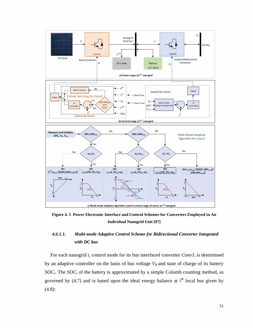
51

Figure 4. 5 Power Electronic Interface and Control Schemes for Converters Employed in An

Individual Nanogrid Unit [97]

4.6.1.1. Multi-mode Adaptive Control Scheme for Bidirectional Converter Integrated

with DC bus

For each nanogrid i, control mode for its bus interfaced converter Conv1i is determined

by an adaptive controller on the basis of bus voltage VB and state of charge of its battery

SOCi. The SOCi of the battery is approximated by a simple Columb counting method, as

governed by (4.7) and is based upon the ideal energy balance at ith

local bus given by

(4.8):

Measure and Initialize SOCi, VB , Vref

SOCi<SOCmin

VB VL

Set Iref=1/Rd*(VL-VB)

Set Ii

ref=Irated*[(SOCi/SOCmin)-1]

SOCi<SOCmax

VB Vref

Set Iref=kc*(Vref-VB)

Set Iref=kd*(Vref-VB)

VB > VH

Set Iref=Irated*[(SOCi-SOCmax)/(100-SOCmax)]

Iiin

Iiload

IiL

VB

Di

VB

di

Control for Conv2i

`

Multi-Mode Adaptive Algorithm for Conv1i

No No

NoNo No

Yes

Yes Yes Yes

Iiload

Set Iref=1/Rd*(VH-VB)

Iiref

PWM

ViPV

MPPT Control

IiPV

Iiin

PI Controller

Iiload

SOCi>SOCmax

andVB VH

SOCi

No

Mode Switching for Conv2i= Signal Flow

= Power Flow

Yes

SOCi

I iref

-Ira

ted

SOCmin

VB

I iref

I rate

d

VL

1/RdVB

I iref

I rate

d

Vref

-Ira

ted

SOCmin

SOCmax

SOCmax

SOCminVB

I iref

I rate

d

VH

1/Rd

SOCi

I iref

I rate

d

100SOCmax

DC Loads Battery

SOCi)

Conv1iConv2i

VB

IiL

PWM

PI Controller

Control for Conv1i

SOCi

Vref

Multi-ModeAdaptive Algorithm

(Vib,

nanogridlocal bus

DC Bus

a) Power stage of ith nanogrid

b) Control stage of ith nanogrid

c) Multi-mode adaptive algorithm used in control stage of conv1 at ith nanogrid

PV Panel Isolated Bidirectional Converter

Buck Converter

52

tdIIIVC

SOCtSOC

T

L

i

load

i

in

i

b

i

i

ii 0

1

0 (4.7)

tdIIIVttPttPttP

T

L

i

load

i

in

i

b

i

L

i

load

i

PV

i 0

(4.8)

Where, SOCi(0) is the initial state of charge for the battery at ith

nanogrid, Ci is its

rated energy capacity (Wh), Iiin

is the current provided by PV panels after buck converter

(Conv2i), Ilload

is the current demanded by household DC loads, IiL is the current supplied

by the nanogrid to the DC bus, PiPV

(t) is the power generated by PV panel at time t whose

rated capacity is PPV

(Wp), Piload

(t) is the power demanded by household at time t whose

rated load capacity is Pload

(W) and Vib(t) is the time varying voltage of the battery whose

rated voltage is Vb. By convention IiL and Pi

L values are positive, when current and power

is being supplied by the nanogrid to the DC bus and negative when current and power is

being demanded by the nanogrid for household load or battery charging. SOCi of the

battery is considered as the resource availability index in this distributed structure. In

order to ensure the coordinated operation along with enhanced battery life time, upper

and lower threshold on the battery state of charge are defined as SOCmax and SOCmin. A

value of SOCi below SOCmin indicates that individual nanogrid is deficient in resources

and any further discharge below this point will badly deteriorate the battery life. So,

individual household loads must be shut down with the help of a relay and it must start

absorbing power to achieve the minimum sustainability level i.e. SOCmin. An inner loop

current control is used to govern the control of the converter through PI controller such

that the deficient nanogrid may demand power in accordance with its extent of

deficiency. In order to maintain the voltage of the microgrid within the stable higher and

lower limits i.e. between VH and VL (generally taken ± 2 to ±5 % of the rated bus voltage

Vref), following droop conditions are employed for SOCi < SOCmin

LB

LB

min

VV if N][1,i ; 1

VV if N][1,i ; 1

BL

d

ref

i

i

rated

ref

i

VVR

I

SOC

SOCII

(4.9)

53

Where, Irated is the rated charging current for the battery, specified by manufacturer

datasheet and Rd is the virtual droop resistance based upon the power ratings of the

converter.

Similarly, a value of SOCi higher than SOCmax indicates that nanogrid has very

high resource availability and needs to supply power to the neighboring nanogrids based

upon the acceptability condition of the microgrid dictated by its upper acceptable voltage

limit VH. Therefore, for SOCi > SOCmax

HB

HB

max

max

VV if N][1,i ; 1

VV if N][1,i ; 100

BH

d

ref

i

i

rated

ref

i

VVR

I

SOC

SOCSOCII

(4.10)

In between SOCmax and SOCmin thresholds, the control of the converter is dictated by

SOC based adaptive IV droop function. For VB higher than Vref, net power supplying

nanogrids are more than the net power demanding nanogrids, therefore, for this condition;

ith

nanogrid needs to absorb power to keep the microgrid stable. However, in order to

make this a coordinated power sharing, the charging droop coefficient Kc has been defined

as a function of droop resistance Rd and SOCi, such that among all the nanogrids in this

range, the nanogrid with relatively lower state of charge absorbs higher amount of power

in comparison to the other nanogrids. The droop coefficient in this range has been varied

linearly between 0.5 Rd to Rd from SOCmin to SOCmax. Other linear and non- non-linear

variations of droop function can also be considered, such that it does not violate the

stability conditions for microgrid operation [66]. This trend is also shown in Figure 4.5

(c).

minmax

min2

1,

SOCSOC

SOCSOC

RSOCRK

i

d

idc (4.11)

Similarly, for VB lower than Vref, each individual naogrid has to supply power in

accordance to its resource availability index. For this range discharging droop co-efficient

Kd as a function of SOCi and droop resistance Rd is given by (4.12) and is also shown in

54

Figure 4.5 (c). In this case, the nanogrid with highest resource availability (SOC) will

supply more in comparison to the nanogrid having relatively lower SOC.

minmax

min1

1,

SOCSOC

SOCSOC

RSOCRK

i

d

idd (4.12)

Based upon (5) and (6), the SOC based I-V adaptive droop control in the range of SOCmin

≤ SOCi ≤ SOCmax is shown in Figure 4.5 (c) and expressed as follows:

refB

refB

VV if N][1,i ;

VV if N][1,i ;

Brefc

ref

i

Brefd

ref

i

VVKI

VVKI

(4.13)

If all the converters are within this range of operation, there will be zero current

sharing among the contributing nanogrids. Therefore, DGDSA implementation with this

type of control will offer minimum distribution losses.

An adaptive algorithm for the calculation of Iiref

based upon (4.9) - (4.13) and local

measurements of VB and SOCi dictates the mode of operation as shown in Figure 4.5(c).

An inner loop current control is then used to control the current of Conv1i through PI

controller that generates the duty cycle Di given by (4.14), where, kp and ki are the

proportional and integral constants for PI controller respectively.

t

L

i

ref

ii

L

i

ref

ipi dtIIkIIkD0

(4.14)

4.6.1.2. Scheme for Switching between MPPT and Current Control Modes for the

Converter Integrated with PV Panel

The buck converter of each nanogrid (Conv2i) at the output of PV panel is

responsible for optimal battery charging. Maximum power point tracking (MPPT) control

is widely used in PV based systems for the extraction of maximum power out of incident

solar energy. Various schemes for MPPT under uniform and non-uniform irradiance have

been discussed in the literature [73, 74]. In this article, the perturb and observe algorithm

is employed due to its simplicity and low computational complexity [73]. The algorithm

processes PV panel voltage ViPV

and current IiPV

to generate duty cycle di for maximum

power extraction from PV panel at a given solar irradiance. In most of its operation range

55

Conv2i will operate in MPPT mode however, based upon the measurements of SOCi and

VB, Conv2i may shift its operation from MPPT mode to inner loop current control mode

such that it culminates its power generation from MPPT to household load current

requirements Iiload

only. Thus, for SOCi > SOCmax and VB ≥ VH, Conv2i will operate in

inner loop current control mode through a PI controller that will generate duty cycle di

given by:

t

in

i

load

ii

in

i

load

ipi dtIIkIIkd0

'' (4.15)

where, kP’ and ki

’ are proportional and integral constants of PI controllers employed for the

control of conv2i.

4.7. Results, Discussions and Conclusions for Adaptive Decentralized Control

For the validation of proposed scheme various test cases are analyzed via

simulations and hardware in loop (HIL) facilities in the laboratory.

4.7.1. Simulation Results for Decentralized Control

Simulations are carried out on MATLAB/Simulink using physical models of the

converters and control schematic shown in Figure 4.5 (c). Various parameters for

simulation are shown in Table I. In order to have a better illustration of results, PiPV

(t) is

assumed equal to Piload

(t) for test case 4.7.1.1 to 4.7.1.3.

4.7.1.1. All nanogrids are within specified thresholds of SOC

In this scenario, the batteries of all nanogrids are assumed to be within specified

thresholds of SOC i.e. 4 3, 2, 1,i; maxmin SOCSOCSOC i.

This case is evaluated with and without communal load and results for variations

in bus voltage, current sharing among contributing nanogrids and accelerated simulations

(0.5 hr) for SOCi are shown in figures 4.6 and 4.7 respectively. It can be seen that after

starting transient, if there is no communal load, current sharing among the nanogrids is

almost zero, i.e. each nanogrid is working independently, without supplying or

demanding power from DC bus. So, their SOC‘s remain constant in this region and

56

distribution losses are zero, despite load requirements of each household is being

fulfilled.

At t= 0.025 s, a communal load of 500 W is applied due to which voltage of the

DC bus drops from 48 V to 47.3 V and each nanogrid starts contributing for communal

load based upon its availability index i.e. according to its SOCi value. Therefore, all

nanogrids are supplying power (being discharged) based upon the modified droop Kd(Rd,

SOCi) given by equation (4.12). Consequently, the nanogrid with highest SOC,

contributes more towards communal load and its SOC decreases at a rapid slope in

comparison to other nanogrids in the system. (ΔSOC1 = 1.92% in comparison to ΔSOC4

= 2.52% at the end of simulation).

Figure 4. 6 DC bus voltage VB profile (righy Y-axis) and current sharing among nanogrids (I1L, I2

L,

I3L and I4

L) (left Y -axis) in case 1 (simulation results)

57


(SOC1, SOC2, SOC3 and SOC4) (left Y-axis) in case 1 (simulation results)

Also, it is worth noting that upon a step change on bus loading (communal load

application), the response time of proposed control scheme is very fast and system

achieves new steady state rapidly. Thus the proposed control method exhibits fast

dynamics due to I-V droop method which uses only one controller delay in comparison to

V-I voltage droop which uses two controller delays resulting in relatively slower system

dynamics. The detailed parameters for the simulated case studies are tabulated in Table I.

It is worth mentioning here, that switching frequency fsw is kept 10 kHz in the simulation

case studies. Generally, higher frequencies may result in lower filter requirements in the

converter operation. The selection of fsw in this particular case study is in accordance with

the compatibility of our dSpace based hardware in loop (HIL) setup discussed below.

Power level for individual households is kept 200 W in this case study, which is

relatively higher in comparison to previous case studies discussed in chapter 3, where we

considered power levels in the range of 30-40W. The selection of higher power level is

made to validate the efficacy of proposed control scheme for higher power levels for

improved livelihood level village scale electrification.

58

Table 4. 1 Parameters of Simulated Case Study [97]

Description of the Parameter Symbol Value Description of the

Parameter Symbol Value

No. of Nanogrids/ households N 4 Maximum threshold of

battery SOC SOCmax 80%

DC bus capacitance CB 10mF Minimum threshold of

battery SOC SOCmin 30%

Inductance of each Conv1i L1 500μH Reference voltage for DC

bus Vref 48V

Switching frequency for

Conv1i and Conv2i fsw 10kHz Initial Voltage of DC bus VB0 24V

Rated power of each PV panel PPV

500Wp Lower limit on DC bus

voltage VL 45.6V

Rated household load Pload

200W Higher limit on DC bus

voltage VH 50.4

Battery capacity for each

nanogrid C 2400Wh

Droop Coefficient for

Conv1i Rd 0.218Ω

Rated Charging current for the

battery Irated 10A

Proportional and integral

parameters (Conv1i) kp ,ki

0.33,

15

Rated voltage of each battery Vb 24V

Proportional and integral

parameters (Conv2i) kp

’ ,ki

’ 0.5, 50

4.7.1.2. All nanogrids are within specified thresholds of SOC except one which is below

minimum threshold of SOC

In this scenario, the batteries of three nanogrids are assumed to be within

specified thresholds of SOC, while battery of fourth nanogrid is assumed to be below

minimum threshold of SOC, i.e. min4maxmin ; 3 2, 1,i; SOCSOCSOCSOCSOC i

Results for bus voltage profile, current sharing among contributing nanogrids and

accelerated simulations (1 hr) for SOCi are shown in Figures 4.8 and 4.9 respectively. It

can be observed from these figures that the nanogrid 4 which is deficient in resources is

demanding current as dictated by (4.9). Therefore, nanogrid 4 is absorbing power with a

negative value of I4L=-5.1A

(charging current), and its SOC4 is increasing with a high

slope.

59

Figure 4. 8 DC DC bus voltage VB profile (righy Y-axis) and current sharing among nanogrids (I1L,

I2L, I3

L and I4

L) (left Y-axis) in case 2 (simulation results)



All other nanogrids are supplying power (being discharged) based upon the

modified droop Kd(Rd, SOCi) given by equation (4.12). The modified droop ensures the

coordinated power sharing such that the nanogrid having higher SOC supply more

current in comparison to nanogrid having relatively lower SOC. For instance in figure

4.8, nanogrid 1 with SOC1=35% is supplying 1.2A, nanogrid 2 with SOC2=55% is

supplying 1.6A and nanogrid 3 with highest SOC3=75% is supplying 2A respectively.

Thus resource sharing is set in proportional to resource availability without any physical

60

layer of communication among the contributing resource and decentralized,

communication-less, yet, coordinated control is realized with the proposed scheme. It is

worth noting that sum of three supplying currents is lower than the absorbing current in

microgrid 4. This is in accordance with the energy balance in (4.7) and (4.8) as the

batteries of three supplying nanogrids are at relatively higher voltage in comparison to

demanding microgrid whose voltage is way below rated voltage due to very low value of

SOC.

Figure 4.9 shows the accelerated simulations for one hour SOCi variations in

batteries of four nanogrids. The battery with higher SOC is being discharged at a rapid

rate in comparison to the batteries having relatively lower SOC as evident by the

observation that changes in SOCi values from the start till end of the simulation are

ΔSOC1=2.09%, ΔSOC1=2.61% and ΔSOC1=3.1% respectively (ΔSOC1 < ΔSOC2<

ΔSOC3). This is in accordance to the desired objectives of the control scheme such that

the battery with highest resource availability i.e. battery 1, is supplying more in

comparison to other two supplying batteries which are also supplying in proportion to

their resource availability.


maximum threshold of SOC


specified thresholds of SOC, while battery of fourth nanogrid is above maximum

threshold of SOC, i.e. max4maxmin ; 3 2, 1,i; SOCSOCSOCSOCSOC i .

Therefore, this case evaluates the operation of microgrid with three of the contributing

nanogrids (1, 2, 3) deficient in resources, while fourth one have enough resource

availability to support the resource deficient nanogrids.

Results for bus voltage profile, current sharing among contributing nanogrids and

accelerated simulations (1 hr) for SOCi is shown in Figures. 4.10 and 4.11 respectively.

Since the initial SOC4(0)

is above threshold i.e. 90%, therefore, in this scenario, nanogrid

4 is supplying power as dictated by equation (4.10) with I1L=4.98A, while other three are

absorbing power (their batteries are being charged) based upon the modified droop Kc(Rd,

SOCi) given by equation (4.11).

61


L,

I3L and I4


Figure 4. 11 DC bus voltage VB profile (right Y-axis) and battery SOC for contributing nanogrids


It can be observed from Figures 4.10 and 4.11 that power sharing via modified droop

ensures resource distribution based upon the availability index. Therefore, nanogrid with

initial SOC3(0)

=75% (highest SOC and highest resource availability) is being charged

with the lowest current I3L = -1.28A in comparison to nanogrid with SOC2

(0)= 55% and

nanogrid with SOC2(0)

= 35% which are being charged at I2L=-1.73A and I3

L =-2.18A

respectively. Moreover, the changes in SOCi from start till end of the simulation are also

in accordance with the modified droop given by equation (4.11) and shown in Figure 4.5

(c), such that ΔSOC1=0.96%, ΔSOC1=0.49% and ΔSOC1=0.2% respectively (ΔSOC1 <

ΔSOC2< ΔSOC3).

62

4.7.1.4. Multi-mode switching of an individual nanogrid

In order to realize the working of an individual nanogrid in all possible threshold

ranges and to visualize the multi-mode switching based upon the SOC thresholds,

nanogrids 2,3 and 4 are considered to be working within specified maximum and

minimum thresholds of SOC with SOC2<SOC3<SOC4 while, nanogrid 1 is considered

below threshold in the start of simulation. It is assumed that PV power produced within

the first three nanogrids is in accordance with their household load requirements; while

incident irradiance and associated PV power produced within nanogrid 1 is higher than

its household load requirements. Therefore, based upon the energy balance given in (4.7)

and (4.8), SOC1 will increase from values below SOCmin to values above SOCmax,

Consequently, Conv11 will switch its operating modes accordingly.

Figure 4.12 shows the variations in current sharing among contributing nanogrids

(I1L, I2

L, I3

L and I4

L) based upon the accelerated SOC variations of an individual nanogrid

(SOC1). Accelerated SOC variations at nanogrid 1 are achieved by considering reduced

battery capacity (C/5) and high incident irradiance (1000W/m2). It can be observed that

when SOC1<SOCmin, nanogrid 1 is demanding current with negative value of I1L as

dictated by equation (4.12). Current demanded by naogrid 1 I1L

decreases as SOC

increases and becomes almost zero upon reaching SOC1 =SOCmin=30%.

It is worth noting that within this range of operation, the current supplying

capability of the remaining three microgrids is governed by the modified discharging

droop Kd(Rd, SOCi) (given by equation (6) and its visual representation is also shown in

Figure 4.5 (c), such that nanogrid 4 having highest SOC is supplying maximum current,

while nanogrid 2, having lowest SOC is supplying lower current. In mid operation range,

i.e. within specified limits of thresholds, all nanogrids are sharing zero current, therefore,

in this range distribution losses are comparatively negligible. Also, the inter-mode

transition is very fast and smooth with the proposed strategy. For SOC1>SOCmax,

nanogrid starts supplying current in accordance with (4.10) and value of I1

L keeps on

increasing with increase in SOC1. Therefore, out of current demanding nanogrids,

nanogrid 2 with the lowest SOC is demanding the highest current while nanogrid 4 with

the highest SOC is demanding the lowest amount of current.

63

Figure 4. 12 Nanogrid 1 SOC1 variation in the various thresholds ranges (left Y-axis) and associated

current sharing among the contributing nanogrids in case 3 (right Y- axis) (simulation results)

4.7.1.5. All nanogrids are above maximum threshold of SOC and surplus PV power is

available

In this scenario, critical conditions of islanded operation are evaluated by

considering that all the nanogrids are above maximum threshold and surplus PV power is

available due to high incident irradiance (1000W/m2) i.e. 4, 3 2, 1,i; max SOCSOCi .

Each naogrid will tend to supply power to the DC bus based upon the equation (4.10),

therefore, its voltage will rise until it reaches to VH. At VH, the proposed droop function

will reduce the current supply to zero and will try to keep the voltages fixed at VH. Since,

the batteries are already above maximum threshold, therefore, any local PV generation

PiPV

, higher than local household requirements Piload

will overcharge the battery and

cause DC bus voltage to rise above the maximum limit VH, thus instigating instability in

the system. At this point, the control schematic of conv2i changes its control from MPPT

to inner loop current control mode as shown in Figure 4.5 (c). Therefore, IV droop

control mode (constant droop coefficient Rd) of Conv1i stabilizes the DC bus voltage at

VH and Conv2i ensures stability by culminating generation capability of each nanogrid

according to the load requirements at individual household level.

64

Figure 4.13 shows that when DC bus voltage is below maximum threshold VH,

each nanogrid contributes for current according to its SOCi. Once the voltage reaches to

VH, current contribution from each nanogrid becomes zero, and further rise in voltage is

restricted to VH. Before attaining VH, each Conv2i is operating in MPPT mode, thus

extracting maximum power (500 W at incident irradiance of 1000 W/m2). However, once

DC bus voltage attains its maximum value VH, the PV generation is limited according to

household load requirements.


L,

I3L and I4


Figure 4. 14 Power generated by PV panels in nanogrid 1 P1PV

(righy Y-axis) and output current I1in

of conv21(left Y-axis) in case 5 (simulation results)

65



This is shown in figure 4.14, where Conv21 of nanogrid 1 is working in MPPT

(P&O) mode and generating power around 500W in the start of simulation. At t=0.027s,

VB reaches to its maximum allowable limit, therefore, Conv2i shifts is control from MPPT

to current control mode, therefore, the output current of conv2i i.e. I1in

coincides with load

current I1PV

waveform as shown in Figure 4.14. This has been also shown in figure 4.15

where, SOCi of each converter is increasing due to PV generation higher than load

requirements, when VB is below VH. After VB becomes equal to VH, due to change in

control mode of Conv21 and associated limited PV generation, the SOC of the battery

does not rise any further and becomes constant onwards.

4.7.1.6. All nanogrids are below threshold of SOC and PV generation is not available

In this case the batteries of all nanogrids are assumed to be below threshold level

and PV generation is not available i.e. 4, 3 2, 1,i; min SOCSOCi . This is the typical case

at night or in cloudy days when no sunlight is available for PV power production.

Since PV generation is not available and all the batteries are already blow

minimum threshold SOCmin, therefore, any local load demand can further discharge

batteries and cause DC bus voltage to collapse below minimum threshold level VL.

66



Therefore, all the local loads are turned off in this condition through a relay and

DC bus voltage is limited to lower threshold of voltage VL through IV droop with

constant droop coefficient as shown in figure 4.5 (c). Thus, any further power sharing

among the contributing nanogrids is restricted to maintain the bus voltage level and

battery SOCi level of individual batteries as shown in figure 4.16. This condition is

maintained until PV irradiance and associated PV generation is available again to charge

the batteries above SOCmin. Thus the proposed control scheme ensures stability even in

the critical conditions of operation, while maintaining the voltage across the grid at lower

threshold limit.

4.7.2. Experimental Results for the Validation of Proposed Adaptive Algorithm for Conv2i

In order to realize various power sharing scenarios during normal operation of

microgrid and to validate the proposed decentralized control scheme, an hardware in loop

(HIL) experimentation is conducted using Danfoss converters and dSpace RTI 1006

platform in Aalborg University (AAU), microgrid laboratory capable to perform real time

data acquisition and control operations [98].

The functioning of adaptive algorithm for the control of Conv1i (shown in Fig. 2.5

(c)) is evaluated using HIL experimentation whose schematics and hardware setup is

shown in figures 4.17 and 4.18 respectively. PV power is emulated using power supply

and battery model is emulated using (4.7) and (4.8). Since functioning of Conv2i is to

67

ensure optimal PV generation in normal and critical conditions of operation and in the

current setup PV power is being emulated, therefore, control of Conv2i is not

implemented for experimentation. Based upon the output of emulated battery model i.e.

based upon SOCi, adaptive algorithm adjusts the mode of operation for each individual

converter. Various parameters of experimentations are further detailed in Table 4.2.

Table 4. 2 Parameters of Experimental Case Study [97]

Description of the


Description of the


No. of Nanogrids/

households N 3

Maximum threshold of

battery SOC SOCmax 80%

DC bus capacitance CB 3.3mF Minimum threshold of

battery SOC SOCmin 30%

Inductance of each

Conv1i L1 8.6H

Reference voltage for DC

bus Vref 48V

Stray resistance for

Inductors ri 0.1Ω Initial Voltage of DC bus VB0 24V

Switching frequency

for Conv1i fsw 10kHz

Lower limit on DC bus

voltage VL 45.6V

Rated power of each

PV panel P

PV 500Wp

Higher limit on DC bus

voltage VH 50.4V

Description of the


Description of the


Rated household load Pload

200W Proportional and integral

parameters (Conv1i) kp ,ki

0.02,

0.1

Battery capacity for

each nanogrid C 2400Wh

Droop Coefficient for

Conv1i Rd 0.25Ω

Rated charging current

for battery Irated 5A

68

Figure 4. 17 Schematics of experimental setup at microgrid laboratory

Figure 4. 18 Hardware setup for practical measurements

PWM

1

ME

AS

UR

EME

NT

1

ME

AS

UR

EME

NT

2

ME

AS

UR

EME

NT

3

S1

S4

DC

PO

WER

SU

PPLY

Communal Load

C

PWM

2

C

PWM

3

S3

C

Conv11Conv12Conv13

Nanaogrid 3 Nanaogrid 2 Nanaogrid 1

io1vBio2io3

S2

Multi-ModeAdaptive Algorithm

PiPVPi

loadVB*ioi

Emulated Battery Model

SOCio

vBvB

SOCi

dSPACE

Bidirectional Converters

Monitoring Platform

Oscilloscope

DC Load Bank

69

4.7.2.1. All nanogrids are within specified thresholds of SOC

In this scenario, the batteries of all nanogrids are assumed to be within specified

thresholds of SOC i.e. 3 2, 1,i; maxmin SOCSOCSOC i.This case is evaluated with

and without communal load of 135W and results for variations in bus voltage, current

sharing among contributing nanogrids and accelerated simulations (1 hr) for SOCi are

shown in figures 4.19 and 4.20 respectively. Measured results are in accordance with the

simulation results as without communal load, the current sharing among the contributing

nanogrids is almost zero (slightly higher than zero due to ESR of individual capacitors,

which otherwise was zero in case of simulation result due to ideal capacitor) and on

application of communal load the current sharing is in proportional to SOCi value. For

instance, battery of nanogrid 1 with initial SOC10=35% is supplying 0.79 A, battery of

nanogrid 2 with initial SOC20=55% is supplying 1.05 A and the battery of nanogrid 3

having initial SOC30=75% is supplying 1.33 A for communal load application. The

change in SOC from start till end of the simulation is in accordance with the SOC

availability i.e. ΔSOC1 = 0.49 %, ΔSOC2 = 0.66 % and ΔSOC3 = 0.84 %. Also the initial

transition and transition from no load to communal load scenario is fast and smooth as

shown in figuress 4.19 and 4.20 respectively.


I2Land I3

L ) (left Y-axis) in case 1 (measured results)

70


(SOC1, SOC2, SOC3 and SOC4) (left Y-axis) in case 1 (measured results)


maximum threshold of SOC


specified thresholds of SOC, while battery of fourth nanogrid is above maximum

threshold, i.e. max1maxmin ; 3 2,i; SOCSOCSOCSOCSOC i . Results for bus voltage

profile, current sharing among contributing nanogrids and accelerated simulations (1

hour) for SOCi are shown in figures 4.21 and 4.22 respectively.


I2Land I3

L ) (left Y-axis) in case 2 (measured results)

71


(SOC1, SOC2, SOC3 and SOC4) (left Y-axis) in case 2 (measured results)

Results verify that the nanogrid 1 having SOC higher than maximum threshold is the

supplying nanogrid while remaining two nanogrids demand according to their resource

availability i.e. nanogrid 2 with higher value of initial SOC20=60% is absorbing

relatively lower current in comparison to nanogrid 3 having higher value of initial

SOC20=40%. Therefore, change in SOC for absorbing nanogrids from start till end of the

simulation is in accordance with resource availability i.e. ΔSOC2 = 0.95% and ΔSOC3 =

1.2% with (ΔSOC3 > ΔSOC2).

4.7.2.3. Multi-mode switching of an individual Nanogrid

Nanogrids 2 and 3 are considered to be working within specified maximum and

minimum thresholds of SOC with SOC2<SOC3 while, nanogrid 1 is considered below

threshold in the start of simulation. It is assumed that PV power produced within

nanogrids 2 and 3 is in accordance with their household load, while PV power produced

within nanogrid 1 is higher than its household load requirements. Therefore, based upon

the emulated model of battery, SOC1 will increase from values below SOCmin to values

above SOCmax, and Conv11 will switch its operating modes accordingly.

Figure 4.23 shows the variations in current sharing among contributing nanogrids

(I1L, I2

L, and I3

L) based upon the accelerated SOC variations of an individual nanogrid

(SOC1). Accelerated SOC variations at nanogrid 1 are achieved by considering reduced

72

battery capacity (C/10). From Fig. 4.23 it can be observed that for region SOC1 < SOCmin

, nanogrid 1 is demanding current with negative value of I1L and nanogrid 2 and 3 are

supplying in proportion to their SOC, therefore, battery of nanogrid 3 having initial

SOC3(0)

=60% is supplying more current in this region in comparison to nanogrid 2 having

SOC2(0)

=40%. This is in accordance with the simulation results shown in Fig. 5 and IV

droop function as shown in Fig. 4.5 (c). The slope of droop increases with SOC in this

particular region as shown by the arrow in Fig. 4.23 which is in accordance with equation

discharging droop coefficient Kd(SOCi, Rd) given by equation (4.12). Similarly for

intermediate region, when all the batteries are within their limits of threshold, the current

contribution from each nanogrid becomes zero; therefore, it also validates our

consideration of almost zero distribution losses in the range of SOCmin≤SOCi≤SOCmax.

Finally, in the region when SOCi > SOCmax, nanogrid 1 start supplying current with

positive value of I1L, while nanogrid 2 and nanogrid 3 absorb power in proportion to their

resource deficiency.

Current sharing is controlled by charging droop coefficient Kc(SOCi, Rd) given by

equation (4.11) such that nanogrid 3 having SOC3(0)

= 60% is absorbing less current in

this region in comparison to nanogrid 2 having SOC2(0)

=40%. Therefore, the slope of

droop increases with the decreasing SOC as shown in simulation results in figure. 4.12.

Figure 4. 23 Nanogrid 1 SOC1 variations in the various threshold ranges (left Y-axis) and associated

current sharing among the contributing nanogrids (right Y- axis) in case 3 (measured results)

73

4.7.3. General Conclusions drawn from the results of Decentralized Control

An adaptive IV droop method for the decentralized control of a PV/Battery based

distributed architecture of an islanded DC microgrid is presented and its validity is

demonstrated with simulations and hardware in loop experimentation. The stability of

islanded microgrid in critical operation conditions is ensured via controlled

synchronization between generation resources and load requirements. The proposed

control method is highly suitable for the rural electrification of developing regions

because it (i) enables coordinated distribution of generation and storage resources at a

village scale, (ii) reduces distribution losses associated with delivery of energy between

generation and load end; (iii) decentralized controllability omits the need of central

controller and associated costly communication infrastructure, and (iv) enables resource

sharing among the community to extract the benefit of usage diversity at a village scale.

Results have also shown that adaptive IV droop algorithm enables fast and smooth

transitions among various modes of microgrid operation based upon the resource

availability in individual households of the village. Therefore, the implementation of

proposed control method on PV/battery based DGDSA of islanded DC microgrid will

enable high efficiency and better resource utilization in future rural electrification

implementations.

74

5 Optimal Planning and Design of

Low-Voltage Low-Power Solar DC

Microgrids

Along with technical improvements in the structure and operation of new

microgrids, it is also important to optimize the overall system through right selection of

system components. Since major existing commercial scale DC microgrid

implementations involve central placement of resources, therefore, it is important to first

evaluate optimal planning of distribution architecture and sizing of various system

components such as solar panels, batteries and distribution conductors to minimize the

overall system cost. Therefore, this chapter is dedicated to develop a framework for

optimal planning and design of low-power low-voltage DC microgrids for minimum

upfront cost. The analysis is based on a) region-specific irradiance and temperature

profiles, b) distribution loss analysis and c) optimum component sizing (storage,

conductor and PV panel) requirements based upon an energy balance model for a 24-hr

operation. Based upon the presented framework, the merits of tailoring distribution

architecture for maximizing the system utility in the planning of future microgrid

deployments are analyzed [99]. The presented framework is valid for existing central

architectures as well as distributed generation distributed storage architecture presented in

this work [96].

5.1. Need for Optimal Planning and Design of Solar PV based DC Microgrids

Although low-voltage, low-power solar PV-based DC microgrid systems are

becoming popular for off-grid rural electrification, however, formal analysis on optimal

component sizing and loss evaluation is not addressed in the literature. Generic microgrid

systems planned without taking the regional characteristics into consideration are

significantly oversized and are not a good fit for all environments and regions. Thus,

there is a need to plan efficient distribution schemes based upon the detailed loss analysis

75

along with quantification of optimal system sizing incorporating local conditions for

overall cost minimization and enhanced system utilization. Various critical parameters

that affect the optimal sizing of system components needs to be identified and analyzed

for optimal system assessment. The component sizing in a solar based DC microgrid is a

function of overall power requirements at each household, regional profile of temperature

and irradiance and distribution losses incurred in the path of power flow from source end

to utilization end. In order to analyze the impact of distribution architecture on optimal

component sizing, distribution losses to actual structure of the village and spatial

distribution of houses in it must be related. Therefore, in order to design optimal

microgrid systems, quantification of distribution losses with respect to distribution

architectures in line with common settlements must be considered.

Kindly note that the focus in this chapter is on lowest cost topologies for basic

rural electrification. Therefore, power levels of individual households for the optimal

framework analysis are kept 5W and 10W, in accordance to the typical commercially

available microgrid solution e.g. Mera Gao Power (MGP) in India, which supplies 5 W of

electricity to the subscribing households. High power microgrids (with household

provisions for several hundred watts) are generally unviable (due to high up front cost

and lack of micro-financing options) and not commonly implemented for self-sustained

rural electrification. Therefore, we restrict our analysis to low-power and low voltage DC

microgrids which are considered safe for direct touch and potentially do not create any

electric shock or fire hazards when implemented at lower voltage levels (24V and 48V)

with 100W name plate capacity. Importantly, the methodology presented in this work, for

the optimal component sizing and optimal distribution architecture planning, is generic

and equally applicable for higher power DC microgrids. However, lower voltages (24V

and 48V) are not suitable for very high power system, as distribution losses would be

very high for low distribution voltages.

5.2. Common Village Orientations

In order to design an efficient power distribution architecture that ensures the

optimal power flow from source end to load end, it is important to analyze the spatial

76

distribution (orientation) of houses commonly found in villages across the developing

countries. Typically, two main arrangements of houses are found:

a) Linear arrangement in which houses are generally situated alongside a central

street/road.

b) Clustered arrangement in which houses are situated in independent fields or in

clusters of multiple huts/homes [100]. Some other similar orientations also occur such as

Zulu‘s in Southern Africa where people built houses shaped like beehives. They built their

houses in a circular fenced compound forming a cluster [101].

Northern Africa and Namibia show highly clustered settlement and population

distribution patterns [102]. However, in Asia, primarily in South East Asian countries such

as India, Pakistan and Bangladesh, the most common forms of rural settlements is linear

arrangement of houses which are situated across roads in order to facilitate access to

infrastructure facilities, markets and resources [88, 103]. In order to electrify these

villages, generally standard radial systems are installed irrespective of the structure of

village and orientation of houses. However, the distribution efficiency of these systems

can be significantly enhanced by taking the structure of village into account and fitting the

right microgrid distribution architectures on it.

In this work, a system model for these linear architectures is developed and

optimization framework for planning and design of low-power and low-voltage DC

microgrids situated in these linear settlements is formulated. In a clustered non-linear

architecture, houses may not be in close proximity and may exist in clusters which are

wide apart. Therefore, an additional concern of PV resources placement along with power

processing and storage unit (PPSU) placement arises because it directly affects the

distribution losses and associated optimal sizing calculations. Due to inclusion of an

additional objective i.e. optimal placement of PV generation and storage unit, the overall

objective function becomes a combinatorial optimization problem. The work on the

development of framework for optimal sizing of the villages with clustered orientations is

under process and its findings will be shared with the community in future contributions.

77

5.3. Proposed Distribution Architectures for Centralized Linear DC Microgrids

Typically, in order to electrify the linear villages with conventional centralized DC

microgrids, standard radial systems with single generation and storage hub are installed

[20, 23, 104, 105]. However, the distribution efficiency of these systems can be

significantly enhanced by considering a second generation hub if the provision is

available. Based upon the structure of village and spatial distribution of houses, we

propose two broad power distribution architectures. The proposed architectures cover

almost all types of village configuration discussed in section 5.2. Therefore, we consider

linear distribution microgrid architecture with up to two generation and storage hubs.

These proposed structures can then be classified into C- distribution architecture and O-

distribution architecture depending upon the number of generation and storage hubs.

5.3.1. Linearly Distributed C- Architecture

The visual representation for linearly distributed C- architecture is shown in

figure 5.1. Distribution conductors are laid in a linear manner while generation and power

processing and storage units (PPSU) are placed at the start of a village, thus formulate a

C-like structure and is termed as linearly distributed C-architecture. This village

architecture is a simplistic model of villages found commonly in India [20].

Figure 5. 1 Topological Diagram of Linearly Distributed C-architecture with PV Generation and

Power Processing and Storage Units (PPSU) [96, 99]

PPSU

PV Panels

78

5.3.2. Linearly Distributed O- Architecture

Based upon the availability of the land, PV generation unit and PPSU may be

located at both ends of the central street. Thus, such a structure in which conductors are

laid in a linear manner, interconnecting generation and storage at both ends of the house

load formulates a linearly distributed O-architecture DC microgrid (figure 5.2). While

keeping the overall generation and storage capacity the same, the introduction of this

architecture having two similar generation and similar storage units on system enhances

its overall efficiency as discussed in subsequent sections.

Figure 5. 2 Topological Diagram of Linearly Distributed O-architecture with two (PPSU’s)[96, 99]

5.4. Energy Balance Model for Centralized DC Microgrids

In order to design an optimal system, it is important to analyze the system in

terms of load requirements, converter requirements, supply availability, storage size and

loss analysis. In this section we evaluate various loss elements in the operation of

microgrid. These losses mainly include i) panel losses in the PV output due to low

irradiance, soiling and mismatch, ii) Degradation in PV output due to temperature, iii)

DC/DC converter losses, iv) battery charge/discharge cycle losses and v) distribution

losses.

The output produced by PV panels is a function of incident irradiance and

temperature. However, due to panel losses and temperature degradations, output of PV

panel is generally lower than its name plate capacity. Low irradiance losses generally

vary linearly with the peak sun hours (PSH) of the incident irradiance. A mathematical

model to quantify low irradiance loss has been presented in [106]. The degradation in

PPSU

PV Panels

PPSU

PV Panels

79

output characteristics of PV Panels due to soiling and mismatch of cells and temperature,

discussed in [107, 108], are also incorporated. Therefore, considering panel losses and the

temperature degradation effect, S(t) is given by (5.1)

tIAtS tcmPL . (5.1)

Where, Itc is the temperature compensated irradiance and depend upon I(t), and Tcell and

is given by (5.3) [109].

tItTtT ambcell *01875.0 (5.2)

tITtI celltc 0045.0251 (5.3)

The output from PV panels is processed through MPPT DC/DC converter which

incurs losses in PPSU along with further DC/DC losses at the distribution panel of each

house (see figures 5.3 and 5.4). The efficiency of a typical DC-DC converter varies

significantly at low power levels (percentage loading). However, the converter losses can

be linearized and its efficiency can be considered as a constant for majority of its

operational range [110]. For instance Kolar et al. [110] shows that a typical DC-DC

converter exhibits slight efficiency variations (±2%), during its operation in between 25

to 95 percent of its rated output power loading. Therefore, the rating of CPPU converter

is approximated to a fixed value. For variable loading scenarios, detailed analysis on

converter losses may be included using (5.8) and (5.14) for accurate sizing estimations.

Battery charging/discharging cycle efficiency (ηB) depends upon the battery technology

and manufacturer specifications. For the system evaluation, lead acid battery is

considered, while its charging/discharging efficiency is considered constant for the

simplicity of analysis. Distribution efficiency is assessed by calculating distribution

losses in the system through Newton-Raphson Method modified for DC power flow

analysis [79]. Ploss(t) accounts for distribution losses and is a function of a) distribution

configuration in a village, b) distribution voltage level and c) permitted load levels to

each household and must be critically analyze. In order to quantify distribution losses, an

N-house village is modeled as a combination of interconnection resistance of the laid

conductors as shown in figures 5.3 and 5.4 respectively. For each configuration (C or O)

of the village, a unique conductance matrix G can be formulated depending upon the

80

spatial distribution between house and length of conductor laid and is given by (5.4) and

(5.5).

NN

NNN

N

N

RG

G

G

G

G

;

G G

G G

G G

N21

22221

11211

(5.4)

y x;

x; 1

xy

N

yxy

xy

g

ygG

(5.5)

This G-matrix can be used to calculate Ploss and maximal voltage dip (VD) as

discussed in [79] and are given by (5.6) and (5.7).

N

xxyyyxx

N

yxyloss VVVVVVGP

1 12

1

(5.6)

minmax

xx VVVD (5.7)

For energy balance model, we consider a typical village microgrid orientation

consisting of N houses electrified via solar PV panels having maximum power generation

capacity Smax (kWp) and a battery storage system having energy capacity CB (kWh). Solar

PV generation S(t) will vary with time depending upon the input irradiance and ambient

temperature, therefore, battery state of charge and associated state of energy EB(t) will

also vary with time depending upon S(t) and load requirements. Load demand of each

house i at any time is given by Pi(t).Therefore, for any time interval Δt, the balance of

energy at microgrid is given by (5.8)

t 1

tPttPtEttS loss

N

iiiBBMP (5.8)

Where, ηMP is the efficiency of DC/DC converter employed at PPSU responsible for

maximum power point tracking, battery charging and maintenance of distribution voltage

and ηi is the efficiency of DC/DC converter employed at the distribution panel of each

house. Since battery may take energy from PV panels or may supply power to the load at

any time t depending upon the net energy flux in the battery, ΔEB(t) can be positive or

81

negative. ΔEB(t) will be negative in durations of no solar power generation and the stored

energy in the battery will be used to meet the load demand.

5.5. System Model Formulation for Optimal Component Sizing of Centralized

DC Microgrids

In order to optimally size various system components including PV generation

capacity Smax (kWp), battery Storage capacity CB (kWh) and conductor size X (AWG) for

minimum cost of installation, we consider the energy flow diagrams for C- and O-

distribution architectures (as dictated by (5.8)) as shown in figures 5.3 and 5.4

respectively.

Figure 5. 3 System Diagram for Energy Flow in C-architecture with N Houses

1 2 3 N/2

EB(t)Battery

PV output

(N/2)+1 (N/2)+2 (N/2)+3 N

S(t)

ηMP

ηB

ESL(t)

E BL(

t)

g12 g23 gxygxy

gxy gxy gxy

η1 η2 η3 ηN/2

ηN

P1(t) P2(t) P3(t) PN/2(t)

PN(t)

ESB(t)

gxy

82

Figure 5.4 System Diagram for Energy Flow in O-architecture with N Houses

5.5.1. Objective function

The overall optimization problem is therefore, the minimization of objective

function (5.9), subjected to the constraints defined by (5.10) - (5.17).

XtStCT

tB

CSEEEE XBBBLSLSB

3max21

1) , , , , ,( min

,max

(5.9)

5.5.2. Inequality Constraints:

Non-negativity constraints on decision variables

T ; 0 ,0 ,0 ,0 ,0 max SCEEE BBLSLSB (5.10)

Since the battery lifetime is dependent upon its depth of discharge (DOD),

therefore, energy level of the battery EB(t) at any time t is not allowed to go below its

minimum energy level dictated by allowable minimum state of charge SOCmin.

T; min BB CSOCE (5.11)

5.5.3. Equality Constraints

1 2 N/2

EB(t)Battery

PV output

(N/2)+1 (N/2)+2

S(t)

ηMP

ηB

E BL(

t)

g12gxy

gxy

η1 η2 ηN/2

ηN

P1(t) P2(t) PN/2(t)

PN(t)

ESL(t)

ESB(t)

N

EB(t)Battery

PV output

S(t)

ηB

ESB(t)

ηMP

E BL(

t)

ESL(t)

gxy

gxy gxy

83

The constraints on generated solar energy are dictated by (5.12) as the generated

energy can either be used to supply load or to charge the battery including the losses

encountered in the path of power flow.

T; tEtEtS BLSLMP (5.12)

Constraints on battery energy are given by the net balance of influx and out-flux of

energy and are given by (5.16)

T; 1 tEtEtEtEE BLSBBBBB (5.13)

The constraints on load are defined by (5.14) such that load demand must always be

fulfilled either through battery or solar PV output. For constant household power loading

scenario as discussed in the current scope of the work, converter efficiency ηi is

considered constant. Therefore, linearization of load constraints does not result in any

significant loss of accuracy. However, in case of variable household loading, non-linear

accurate models for converter efficiency need to be included for accurate estimations

[110].

T;

11 1

tEtEtPttP

BLSL

T

t

loss

T

t

N

ii

i

(5.14)

The optimal PV size Smax is determined by the maximum output power produced by PV

array. Similarly, optimal battery size CB is determined by the maximum energy state

attained by the battery, therefore, (5.15) and (5.16) dictate the equality constraints

associated with the objective function for the optimal sizing of PV and battery

respectively.

T; )max(max SS (5.15)

T; )max( BB EC (5.16)

A range of possible conductor sizes for DC distribution are considered from

American wire gauge (AWG) table [48]. Therefore, constraints on Conductor size are

given by (5.17).

AWGAWGAWGAWGAWGAWGAWGX 16 14 12 10 8 6 4 ,,,,,, (5.17)

84

For considered range of operation, the stated objective function along with

equality and inequality constraints exhibit linearity as shown by (5.9)–(5.17). Therefore,

optimization problem is written in standard linear form and is solved through linprog

function in MATLAB.

5.6. Results and Discussion for Optimal Sizing of Centralized DC Microgrids

For the current scope of work, we consider a typical linear village structure in

South East Asia having (typically) 40 houses and distance between two consecutive

houses is (typically) 10m. We consider both C- and O- architectures along with two

distribution voltages of 24V and 48V. Optimal selection of PV panel size, battery storage

capacity and conductor size is performed for 5W (case 1) and 10W (case 2) provision and

is based upon problem formulated in section 5.6.

The idea is to account for the impact of instantaneous fluctuations in PV

generation (based upon timed fluctuations in instant irradiance and temperature) and

losses on system sizing, therefore, selection of time base is critical. Selection of smaller

time base results in better resolution to account for instantaneous changes, however,

requires more computational resources for data processing. The proposed methodology is

generic and can be applied for any time base, based upon the availability of solar

irradiance data, load profile and computational resources for optimization problem

solving. For current optimization problem, discrete time interval of 1 hour with constant

load demand for each house is used as time base for all the calculations. Hourly

variations in the irradiance and temperature data are taken from NREL [49]. According

to the presented optimization problem optimal PV, battery and conductor sizing is

determined.

PV panel shading losses are considered 8% for both cases. Although the converter

losses are quadratic in nature but due to fix load assumption and for simplicity in

optimization problem formulation, DC-DC converter losses for CPPU as well as

individual household distribution panel converter are considered 10% for both cases.

Battery cycle efficiency ηB is considered 95%, and is assumed constant for simplicity of

analysis. The cost of panels per watt-peak ‗w1‘is taken as 600$/kWp (including the cost

of mounting frame) and lead-acid battery cost per kWh ‗w2‘ is taken as 120$/kWh and

85

gauge sizes cost is taken at 1671, 1305, 947, 588, 358, 250 and 204 $ for 4, 6, 8, 10, 12,

14 and 16 AWG, respectively [50, 111, 112]. While there are variations in these costs but

we took most commonly found prices at which sourcing is readily available. For overall

system cost calculation, fixed cost of 300$ has been included which accounts for CPPU

and converter cost.

5.6.1. Case 1: 24-7 5W Supply to 40 Houses for a 365-day Operation

Based upon the analysis presented in section 5.5, the distribution efficiency, ηD

and worst voltage dips, VD calculated for following cases are plotted in figure. 5.5.

i. C-24V (C-architecture with 24V distribution)

ii. O-24V (O-architecture with 48V distribution)

iii. C-48V (C-architecture with 48V distribution)

iv. O-48V (C-architecture with 48V distribution)

VD is critical in terms of power electronic converter requirement at each

subscribing household. While, generally, a 20% input voltage variation capability is

allowed in most power electronic converters, the performance is optimal close to the

rated input voltages. For this particular analysis, we limit the optimum component

selection at 20% variations in the grid voltages. It is also interesting to note that O-24V

and C-48V have similar voltage dips and efficiencies for all wire sizes. This is because of

the uniform loading and equal generation at both ends of the O- architecture. In case of

non-uniform loading and unequal generation, the characteristics of C-24V and O-48V

will not necessarily resemble, therefore, detailed distribution loss analysis has to be

performed as discussed in [79]. Along with the selection of PV panel and battery size,

one important parameter is the optimization of the conductor size. The cost of conductor

increases with its decreasing gauge thickness and vice versa while an opposite trend for

system distribution efficiency is observed. Therefore, in order to analyze this effect in

terms of cost, figure. 5.6 (based on 365-day study on the solar irradiance data of Bihar,

India) is plotted. The cost of distribution losses is calculated by taking the difference

between overall system cost with distribution losses at a particular AWG and the overall

system cost with ideal conductor having zero distribution losses.

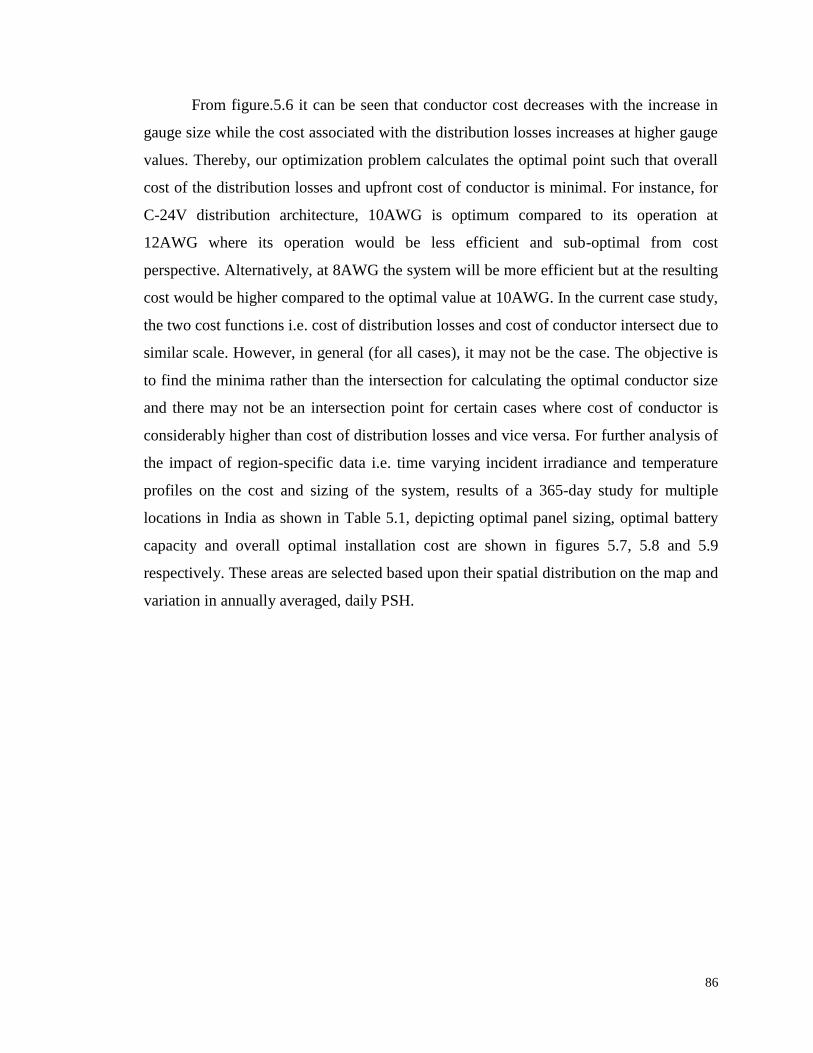
86

From figure.5.6 it can be seen that conductor cost decreases with the increase in

gauge size while the cost associated with the distribution losses increases at higher gauge

values. Thereby, our optimization problem calculates the optimal point such that overall

cost of the distribution losses and upfront cost of conductor is minimal. For instance, for

C-24V distribution architecture, 10AWG is optimum compared to its operation at

12AWG where its operation would be less efficient and sub-optimal from cost

perspective. Alternatively, at 8AWG the system will be more efficient but at the resulting

cost would be higher compared to the optimal value at 10AWG. In the current case study,

the two cost functions i.e. cost of distribution losses and cost of conductor intersect due to

similar scale. However, in general (for all cases), it may not be the case. The objective is

to find the minima rather than the intersection for calculating the optimal conductor size

and there may not be an intersection point for certain cases where cost of conductor is

considerably higher than cost of distribution losses and vice versa. For further analysis of

the impact of region-specific data i.e. time varying incident irradiance and temperature

profiles on the cost and sizing of the system, results of a 365-day study for multiple

locations in India as shown in Table 5.1, depicting optimal panel sizing, optimal battery

capacity and overall optimal installation cost are shown in figures 5.7, 5.8 and 5.9

respectively. These areas are selected based upon their spatial distribution on the map and

variation in annually averaged, daily PSH.

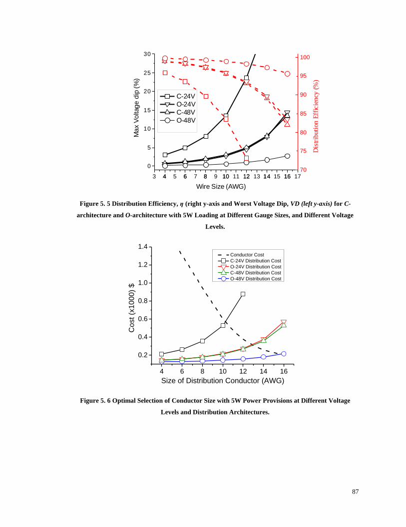
87

Figure 5. 5 Distribution Efficiency, η (right y-axis and Worst Voltage Dip, VD (left y-axis) for C-

architecture and O-architecture with 5W Loading at Different Gauge Sizes, and Different Voltage

Levels.

Figure 5. 6 Optimal Selection of Conductor Size with 5W Power Provisions at Different Voltage

Levels and Distribution Architectures.

3 4 5 6 7 8 9 10 11 12 13 14 15 16 17

0

5

10

15

20

25

30

Ma

x V

oltag

e d

ip (

%)

Wire Size (AWG)

C-24V

O-24V

C-48V

O-48V

4 6 8 10 12 14 1670

75

80

85

90

95

100

Dis

trib

uti

on E

ffic

iency

(%

)

4 6 8 10 12 14 16

0.2

0.4

0.6

0.8

1.0

1.2

1.4

Co

st

(x1

00

0)

$

Size of Distribution Conductor (AWG)

Conductor Cost

C-24V Distribution Cost

O-24V Distribution Cost



88

Table 5.1 Specific Regions for Analysis with Irradiance Profiles

Regions Annually Averaged PSH Regions Annually Averaged PSH

1. Bihar 4.992 7. Jhansi 5.457

2. Dehli 5.035 8. Indore 5.493

3. Kolkata 5.063 9. Mumbai 5.604

4. Rajpur 5.280 10. Aurangabad 5.664

5. Ranchi 5.328 11. Jhodapur 5.808

6. Banglore 5.400

Figure 5. 7 Optimal PV Panel Sizing of the System at 5W Loading (Case 1). Kindly, note that each

data point on the figure represents a region shown in table 1. For instance, the first data point (from

left) is for Bihar where PSH is 4.992 and so on. (Followed in all subsequent figures)

5.0 5.2 5.4 5.6 5.81.2

1.3

1.4

1.5

1.6

1.7

PV

Siz

ing (

KW

p)

Average Daily Peak Sunlight Hours (PSH)

C-24V

O-24V

C-48V

O-48V

89

Figure 5. 8 Optimal Battery Sizing of the System at 5W Loading on left Y- axis and Irradiance

Volatility Factor on Right Y- axis (Case 1)

Figure 5. 9 Optimal Installation Cost of the System at 5W Loading (Case 1)

From Fig. 5.7-5.9, a few important observations can be made:

1) Optimal PV sizing varies approximately linearly with the average daily PSH as shown

in figure 5.7.

2) Average daily PSH are not a direct measure for optimal battery sizing (figure 5.8).

5.0 5.2 5.4 5.6 5.84

5

6

7

8

9

10

11

12

13

14

15

16

17

18 C-24V

O-24V

C-48

O-48V

IVF


-10

-5

0

5

10

15

Irra

dia

nce

Vo

latilit

y F

acto

r (%

)

Ba

tte

ry S

izin

g (

KW

h)

5.0 5.2 5.4 5.6 5.8

1.8

2.0

2.2

2.4

2.6

2.8

3.0

3.2

3.4

Optim

al C

ost (x

1000 $

)


C-24V

O-24V

C-48V

O-48V

90

3) As the battery cost constitutes a predominant portion of the overall cost of the system,

the overall cost of the system also does not vary linearly with the daily PSH (figure 5.9).

Figure 5.8 and table 5.1 verify that ―optimal battery sizing is not directly related

with the average PSH and the information of average PSH only is not sufficient for

optimal sizing of battery storage requirements.‖ Rather, a detailed analysis on the

variations pattern of PSH is needed to calculate the optimal battery storage requirements.

For instance, in figure 5.8, for all four cases, the battery requirements are lower for

PSH=5.3 in comparison to PSH=5.4 and PSH=5.5. Thus, if a proper investigation is not

made for daily variations in PSH, it may leads to incorrect sizing estimations. Therefore,

a detailed analysis must be conducted to find the optimal battery sizing incorporating the

volatility of irradiance. In order to analyze this further an irradiance volatility factor

(IVF) has been defined, which accounts for the number of dips from the mean

‗temperature compensated irradiance‘ and their corresponding extent of deviation

normalized over mean irradiance.

DN

i

i

tc

m

tcm

tc

IINI

IVF1

1 (5.18)

Where, N is the total number of temperature compensated irradiance recordings

out of which ND numbers of recordings are below mean temperature compensated

irradiance (Itcm) and (Itc

i) is the temperature compensated irradiance of i

th dip. Using

(5.18), IVF has been calculated for various regions under observation and it is found that

battery sizing varies in direct proportion with IVF as shown in figure 5.8. The value of

IVF depends on number of dips and their extent of deviation from the mean intensity.

IVF directly impacts the battery sizing and in turn the overall cost of the system. For

instance, in figure 5.8, it can be seen that Kolkota with a relatively low PSH 5.06 (table

5.1) compared to Banglore (PSH 5.4) requires lower battery size. This is due to the

reason that Kolkota has lower IVF (volatility factor) compared to Banglore which

directly translates into reduction in the battery size. Similarly, regions with higher IVF

require higher battery sizing despite of possibility of having high mean irradiance.

Therefore, the sizing of a PV system must incorporate the volatility of irradiance along

with the mean values for PSH.

91

5.6.2. Case 2: 24-7 10W Supply to 40 Houses for 365-days Operation

The most critical aspect is the calculation of optimal sizing for higher power

(10W) is the worst voltage dip along with distribution efficiency of each distribution

topology (see figure 5.10). With the increase in power provisioning, the distribution

losses (I2R) increase significantly compared to case 1 (5W household load). However,

like case 1, C-48V and O-24V have very similar voltage dips and overall distribution

efficiencies. Moreover, distribution at lower voltage level i.e. 24V with C-distribution

architecture becomes practically infeasible due to higher losses and higher voltage dips.

The increased distribution losses can be compensated by selecting a thicker

conductor which will increase the cost of the system. Therefore, it becomes even more

critical to optimally size the conductor by taking the capital and relative cost of

distribution into account. The proposed optimization framework therefore, enables the

optimal selection of conductor size based upon the trade-off between cost of the

conductor and its relative cost of distribution (see figure 5.11). From the comparison of

figures 5.6 and 5.11, it can be seen that with the higher power provision, the optimal

conductor selection has been shifted to lower gauge size (thicker conductor).

Figure 5. 10 Distribution Efficiency ηD and Worst Voltage Dip VD for C-architecture and O-

architecture with 10W Loading at Different Gauge Sizes, and Different Voltage Levels

3 4 5 6 7 8 9 10 11 12 13 14 15 16 17

0

5

10

15

20

25

30

C-24V

O-24V

C-48V

O-48V

Max V

oltage d

ip (

%)

4 6 8 10 12 14 1670

75

80

85

90

95

100

Dis

trib

uti

on E

ffic

iency

(%

)

Wire Size (AWG)

92

Figure 5. 11 Optimal Selection of Conductor Size with 10 W Power Provisions based upon the

Relative Cost of Distribution at Different Voltage Levels and Distribution Architectures

For instance, the optimal conductor sizes for 5W operation (figure 5.6) are 10,

12, 12 and 16 AWG for C-24, O-24, C-48 and O-48 configurations respectively. While

for 10W provision, the gauge sizes are reduced to 6, 10, 10 and 12 AWG for C-24, O-24,

C-48 and O-48 configurations respectively. Therefore, the proposed optimization

framework has adjusted the conductor size such that overall cost of the losses has been

compensated by the selection of a thicker conductor while keeping the overall cost of the

system as minimum. Figure 5.12 shows the overall system optimal cost for various

regions (with reference to their PSH). It is important to note that due to the planning

flexibility in the current framework, the overall cost of the system in high power

provision follows the same trend with relatively higher values in comparison to case 1.

Further it has been observed that the overall panel and battery requirements for case 2

also follow a similar trend as compared with case 1 (results for case 2 are not shown

here).

4 6 8 10 12 14 160.0

0.5

1.0

1.5

2.0

Conductor Cost




O-48V Distribution CostC

ost (x

1000)$

Size of Distribution Conductor (AWG)

93

Figure 5. 12 Optimal Installation Cost of the System (case 2)

Based upon the analysis, figure 5.13 shows the spatial distribution of various

regions on the map and associated optimal sizing requirements for PV panel (kWp),

battery sizing (kWh) and optimal system cost. The case for 24V, O-configuration with

5W loading is represented on the map as a sample case. Optimal data map for other

configurations and voltage levels may also be drawn by using the presented analysis.

Figure 5. 13 Optimal Sizing for 24V, 5W, O- Configuration Represented on Map

5.0 5.2 5.4 5.6 5.83.0

3.5

4.0

4.5

5.0

5.5

6.0

6.5

Optim

al C

ost (x

1000 $

)


C-24V

O-24V

C-48V

O-48V

94

5.7. Optimal Component Sizing for Distributed Generation and Distributed

Storage Architecture based DC Microgrids

In case of DGDSA based DC microgrids, the overall energy balance model can be

considered same as that presented for centralized microgrids. The difference in sizing

results primarily due to lower distribution losses in the distributed architecture which

reduces the need of PV generation and battery storage in individual nanogrids. Therefore,

energy balance model for DGDSA of DC microgrid build around a village having N

houses is given by

t 11

,1

tPttPtEttS loss

N

iii

N

iiBB

N

iiMP (5.19)

Where, ηMP is the efficiency of DC/DC converter employed for MPPT of PV panels, ηi is

the efficiency of DC/DC converter employed at the distribution panel of each house, Si(t)

is the time varying solar power generation, ΔEB,i(t) is the time varying change in energy

state of the battery and Pi(t) is the household load demand at individual household i, in

between any time interval Δt.

Due to assumption of constant battery and DC/DC converter efficiency, equation

(5.19) for DGDSA behaves exactly in same manner as equation (5.8) for centralized

architecture, if battery capacity and PV generation capacity on all N houses is considered

identical. Therefore, the optimal component sizing framework presented for centralized

architectures is equally applicable for DGDSA with the aforementioned assumptions. The

only factor which creates the difference is the distribution losses Ploss(t) which is

considerably lower in DGDSA as compared to centralized architecture as discussed in

Chapter 3. Thereby, using the framework presented in section 5.6 and the distribution

loss calculation model for DGDSA with ring-main scheme of interconnection presented

in chapter 3, the overall sizing of N households (PV sizing, battery sizing and conductor

sizing) is calculated. Sample results for 10W rated power at each household for various

voltage levels and various regions under considerations in table 5.1 are shown in figure

5.16-5.18 respectively. It should be noted here that for distribution loss calculation for

DGDSA operation, peak power sharing scenario, where each household may share

±100% of its rated power has been considered.

95

Figures 5.14-5.16 show the optimal PV sizing (kWp), optimal battery sizing

(kWh) and optimal system cost ($) for N houses in DGDSA at 10W rated power with

various voltage levels and various irradiance levels (regions under consideration given in

Table 5.1) respectively. It should be noted that at low voltages i.e. at 48V, the distribution

losses are relatively higher, therefore, PV sizing, battery sizing and system cost is

relatively higher. At higher voltages 120V and above, due to limited power delivery, i.e.

10 W only, the distribution losses are virtually absent due to distributed nature of the

architecture even at peak power sharing scenario, therefore, the associated sizing values

on higher voltages overlap with each other. Moreover, the trend for optimal PV sizing,

optimal battery sizing and optimal system cost is the same as for centralized architecture

of DC microgrid i.e. optimal PV sizing is directly proportional to incident irradiance,

while the optimal values of battery sizing and system sizing depends upon the incident

irradiance pattern, i.e. its mean value, number of dips and their extent of deviation from

mean value, therefore, IVF is a true measure for optimal battery sizing and optimal

system cost for DGDSA based electrification as well.

Figure 5. 14 Optimal PV Panel Sizing for N houses in DGDSA at 10W Loading

5.0 5.2 5.4 5.6 5.8

2.4k

2.7k

3.0k

400 V

325 V

240 V

120 V

48 V


PV

Siz

ing

(K

WP)

2.4k

2.7k

3.0k

96

Figure 5. 15 Optimal Battery Sizing for N houses in DGDSA at 10W Loading

Figure 5. 16 Optimal System Cost for N houses in DGDSA at 10W Loading

5.8. Optimal Component Sizing Comparison between Centralized and DGDSA

based DC Microgrid

In order to have comparison between centralized architecture of DC microgrid

having all of its generation/storage resources placed at a central location and the proposed

DGDSA from optimal component sizing prospective, we have considered the case of

5.0 5.2 5.4 5.6 5.8

6.0k

8.0k

10.0k

12.0k

14.0k

Battery

Siz

ing (

Whr)

400 V

325 V

240 V

120 V

48 V6.0k

8.0k

10.0k

12.0k

14.0k


5.0 5.2 5.4 5.6 5.8

2.7k

3.0k

3.3k

3.6k

3.9k

4.2k

Op

tim

al C

ost

(x1

$)

400 V

325 V

240 V

120 V

48 V


2.7k

3.0k

3.3k

3.6k

3.9k

4.2k

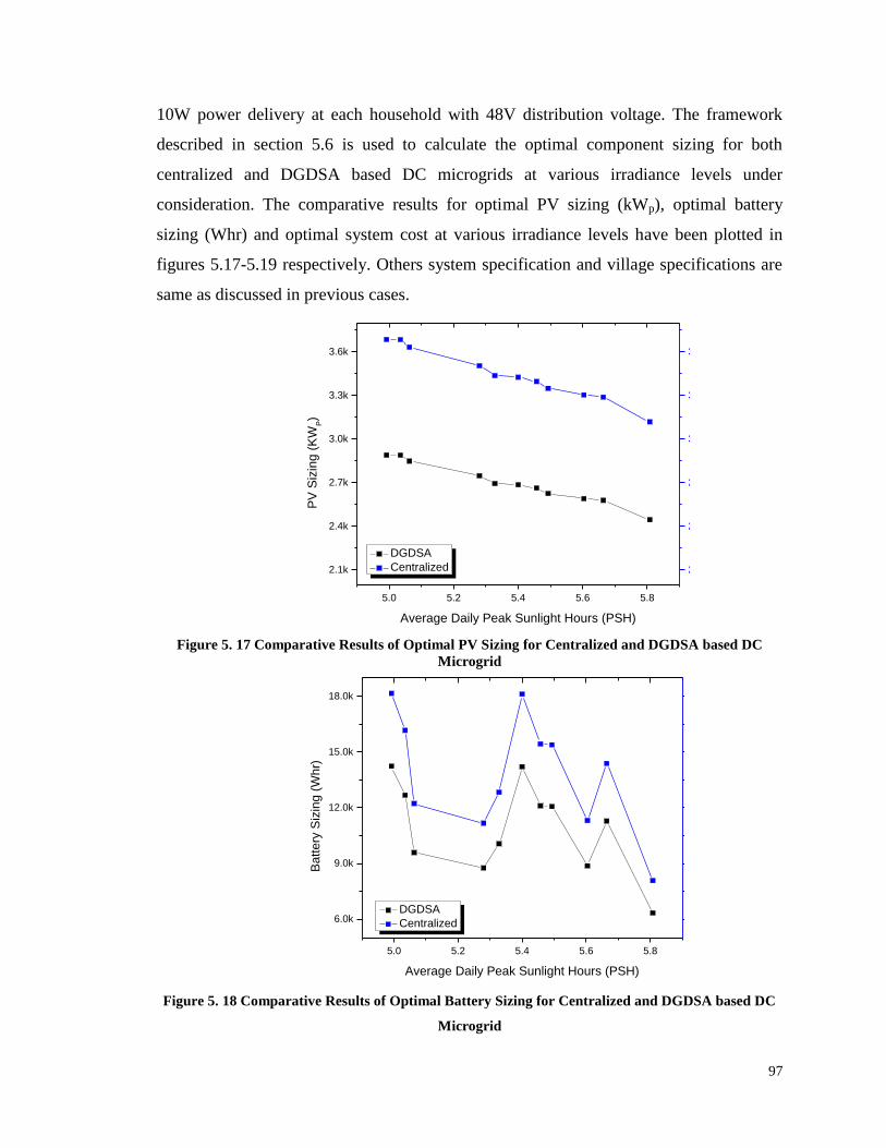
97

10W power delivery at each household with 48V distribution voltage. The framework

described in section 5.6 is used to calculate the optimal component sizing for both

centralized and DGDSA based DC microgrids at various irradiance levels under

consideration. The comparative results for optimal PV sizing (kWp), optimal battery

sizing (Whr) and optimal system cost at various irradiance levels have been plotted in

figures 5.17-5.19 respectively. Others system specification and village specifications are

same as discussed in previous cases.


Microgrid

Figure 5. 18 Comparative Results of Optimal Battery Sizing for Centralized and DGDSA based DC

Microgrid

5.0 5.2 5.4 5.6 5.8

2.1k

2.4k

2.7k

3.0k

3.3k

3.6k

DGDSA

Centralized


PV

Siz

ing

(K

WP)

2.1k

2.4k

2.7k

3.0k

3.3k

3.6k

5.0 5.2 5.4 5.6 5.8

6.0k

9.0k

12.0k

15.0k

18.0k

DGDSA

Centralized


Battery

Siz

ing (

Whr)

6.0k

9.0k

12.0k

15.0k

18.0k

98


Microgrid

From figures 5.16-5.19 it may be concluded that due to relatively lower

distribution losses in DGDSA, the optimal component sizing requirements are relatively

lower in DGDSA in comparison to centralized architecture. Therefore, from optimal

system planning and design prospective, DGDSA is a better choice for future rural

electrification.

5.0 5.2 5.4 5.6 5.8

2.8k

3.2k

3.6k

4.0k

4.4k

4.8k

5.2k

DGDSA

Centralized


Optim

al C

ost (x

1$)

2.8k

3.2k

3.6k

4.0k

4.4k

4.8k

5.2k

E2

99

6 Conclusions and Future Work

Based upon the work presented in previous chapters, general conclusions are

drawn in this chapter. Moreover, the challenges associated with the practical

implementation of the proposed microgrid architecture are also highlighted. Although the

work presented in this thesis conducts the technical investigation, the economic aspects

associated with the installation, operation and maintenance needs to be investigated.

Since it is envisioned that the proposed architecture will have practical implementation in

developing countries, therefore, a framework for economic analysis is currently being

worked out to ensure wide adoptability of the proposed technology. This aspect is further

highlighted in this chapter.

6.1. Conclusions

General findings from the perspective of architecture, control and optimal planning are

detailed and guidelines for future implementations are outlined in this section.

Distributed Generation and Distributed Storage Architecture of DC Microgrid is an

Optimum Technical Choice for Rural Electrification

This work presents a novel DC microgrid architecture for rural electrification with

emphasis on power provisioning beyond subsistence level [71]. The proposed microgrid

is formulated through the interconnection of multiple nanogrids, where an individual

nanogrid is the integral part of the overall microgrid structure. Each nanogrid has its own

PV generation, battery storage and also has the capability of bidirectional power

exchange with neighboring microgrids. Resource sharing allows the consumers to pool

up power for running high power community loads. The proposed microgrid built

through bottom-up cluster of multiple nanogrids is therefore scalable and also has the

capability to extract the benefit of usage diversity due to its resource sharing nature. The

distributed nature of PV generation and battery storage resources result in lower

distribution losses in comparison to existing centralized architectures of DC microgrids

for rural electrification. Using the Newton-Raphson method for modified DC power flow

100

analysis, various power provisioning scenarios for nanogrids and communal load are

evaluated. The validation of the proposed methodology is also done through a scaled

down version of hardware. Based upon the results, it has been concluded that by

increasing the distribution voltage level, distribution efficiency can be enhanced;

however, higher voltages result in enhanced system complexity form protection and

safety point of view. Although lower voltages are considered more safe and do not

require sophisticated schemes for safety and protection, but considerable distribution

losses are associated with power delivery at lower voltages. The choice for optimal

distribution voltage level can be made based upon the trade-off between the cost of

distribution losses, distribution conductor and protection equipment. Central architectures

incur very high distribution losses at high power delivery, therefore, are limited to low

power applications and are not suitable for high power community load operations. The

results of analyses show that the proposed distributed storage architecture can enhance

distribution efficiency by approximately 5% more than other LVDC architectures. The

analysis showed that for the selected parameters, the distribution losses were less than 3%

even at a communal load of 400 W.

Decentralized Control is an Excellent Candidate Solution for Communication-less

Coordination among the Resources in Distributed Microgrids

Centralized architectures are relatively simpler from installation, control and

operation prospective, however, they lack modularity and significant distribution losses

are associated with their delivery of energy. Distributed architectures on the other hand

are scalable, modular and have lower distribution losses; however, they require

sophisticated control techniques involving communication among the distributed

resources for their stable operation. Alternately, in this thesis, a communication-less

control strategy for the stable operation of a PV/battery-based highly distributed

architecture of DC microgrid is presented. A decentralized control scheme is developed

for the communication-less, yet coordinated control among the distributed resources

using multi-mode adaptive IV droop method, relying on local information of DC bus

voltage and battery SOC at individual nanogrids. The efficacy of the proposed control

scheme is validated for various possible power sharing scenarios using simulations on

101

MATLAB/Simulink and hardware in loop facilities at microgrid laboratory in Aalborg

University. The proposed control method is highly suitable for the rural electrification of

developing regions because it (i) enables coordinated distribution of generation and

storage resources at a village scale, (ii) decentralized controllability omits the need of

central controller and associated costly communication infrastructure, and (iii) enables

resource sharing among the community to extract the benefit of usage diversity at a

village scale.

Optimal Planning and Design of DC Microgrid sizing can significantly reduce the

system costs

In this thesis, a planning framework is developed to find the optimal component

sizing for various components of a DC microgrid ensuring minimum cost of installation

[113]. To analyze the impact of distribution architecture on optimal component sizing,

distribution losses are related to actual structure of the village and spatial distribution of

houses in it. For centralized microgrids, two possible architectures of DC distribution (O-

architecture and C-architecture) have been analyzed for power flow and associated

distribution losses. It has been identified that optimal sizing of the system components is

highly dependent upon region-specific time varying profile of irradiance and temperature

throughout the year. The proposed framework allows optimal selection of 1) solar panel

sizing, 2) storage size and 3) conductor size for optimal cost solution. The selection of

distribution voltage and the distributed architecture is ultimately the choice for the

microgrid installers/planners and is influenced by power converter preferences and

financial models. But, importantly, the framework established in this work for optimal

system topology (in multiple constraint scenarios) will be highly useful in planning for

new optimal low-voltage systems along with efficiency enhancements of many existing

systems by retrofitting distribution architectures. Also, it has been found that distributed

generation, distributed storage architecture results in lower distribution losses, lower

system sizing and lower installation cost for same power delivery in comparison to

centralized architecture.

102

6.2. Potential Challenges in Practical Deployments of Decentralized Microgrids

Although the proposed architecture allows for the efficient utilization of

distributed resources in a highly scalable manner, some challenges associated with larger

deployments persist. High-level distribution of resources poses a challenge with respect

to safety and protection due to the increased likelihood of short circuit contribution from

multiple paths within the microgrid. Therefore, future large-scale practical

implementations must include an intelligent protection scheme capable of real-time load

flow and short circuit analysis for adaptive relay settings (not part of the scope of this

study). Further work on the islanded operation of the microgrid is also important to

ensure optimum isolation from the grid for enhanced safety.

From the perspective of control, although hysteretic-based voltage droop control

can reduce multiple layers of sensing and control in the DGDSA, for large-scale

implementations, additional sensing and hierarchical control layers may be added to

ensure the enhanced stability of the microgrid over a wide range of operations.

From practical implementation prospective, there can be potential challenges for

the distributed placement of resources. Space barriers along with the maintenance of

converters and cleaning of PV panels at individual households are some of the practical

challenges that need to be addressed for successful practical implementations. Bi-

directional power flow metering and theft monitoring issues must also be considered for

future installations.

From economics point of view, such a distributed model is highly suitable for

micro-financing opportunities for private investors / public-private partnerships and many

successful models exist in practical as well as in literature highlighting the role of micro

financing in energy access [114]. The participation of the private sector has grown in

recent years [115] but more needs to be done. For instance, experience of past rural

electrification projects in South Asia suggests subsidized micro-financing schemes for

local communities along with public/private partnerships for the successful

implementation of such projects [116, 117]. Therefore, Technical innovations must be

coupled with suitable business models to ensure wide uptake of energy-related initiatives.

103

6.3. Cost and Affordability Evaluation of the Decentralized Microgrid System

Although rural electrification through PV based DC microgrids has been widely

adopted as a successful solution for providing basic electrification in off-grid

communities throughout the world, however, in context of Pakistan, there exists some

potential barriers related to sophisticated demand and policy implementation that needs to

be considered for wide deployment of distributed microgrids. Therefore, a thorough

economic analysis along with a suitable business model for its wide uptake must be

investigated. The work on a demand based decentralized electrification model in

collaboration with International growth Center (IGC), UK is under progress. Focus of the

project is to assess ‗willingness to pay‘ for certain electricity services and how consumers

would behave when the actual system is rolled out. The work in this aspect is still

ongoing and findings of the project including financial model to support micro financing

in the sector of energy along with associated energy policy recommendations will be

shared with academic community in due course. A brief highlight of the work under

progress is discussed in the following sub-sections.

6.3.1. Survey Data

A household census was carried out across 7 villages in the Multan district of

Punjab, Pakistan. The surveys covered all 140 households in the area that were

designated as off-grid, i.e. they are not covered by the national electricity grid. Other than

basic household characteristics, the survey elicited willingness to pay for different

bundles of electricity services, to gauge the demand for such services. Finally, the survey

elicited whether households would be willing to pay for three different levels of

electricity service, provided through microgrids. Levels of service were chosen to

replicate services provided by traditional microgrids, such as Mera Gao Power, and those

made available through the use of distributed architecture of microgrid. The prices at

which these services were offered were randomized between three rate plans, which

presented increasing prices for each level of service. Due to the close proximity of

households inside each village, plans were randomly allocated at the village level, instead

of the household level. Table 6.1 provides details of the level of services and their

respective prices per month under each price plan.

104

Table 6. 1 Services offered and their prices by plan

Level of service Prices

Price plan 1

(USD/month)

Price plan 2

(USD/month)

Price plan 3

(USD/month)

1 24/7 provision of high quality light (3 LED

lights), and a mobile charging point.

1.5 2.5 4.5

2 Services in Bundle 1 and a Fan. 3.0 5.0 9.0

3 Services in Bundle 2 and shared communal

load (water pump).

4.5 7.5 10.5

6.3.2. Survey Results

Table 6.2 presents summary statistics for the reported prices for each level of

service, and also separates it by price plan. We find that not only is demand for the level

of services significant in our sample villages but demand for higher levels of service is

significantly more than for basic electrification. Table 6.3 reports the absolute and

relative difference in prices respondents reported they were willing to pay with respect to

the base level of electrification (lights only), where, absolute difference is the arithmetic

difference in prices of two packages (Py – Px), and relative difference is their ration

(Py/Px).

Table 6. 2 Average Prices Willing to be Paid for Each Level of Service

Average Price/month in USD (standard error)

Number of

Households

Lights Only Lights and Fan Lights, fan and

communal load

Overall 122 1.87

(0.98)

3.40

(0.16)

4.35

(0.17)

Price plan 11 22 1.5

(0)

3.0

(0)

4.5

(0)

Price plan 2 56 1.53

(0.69)

2.94

(0.12)

3.8

(0.12)

Price Plan 3 44 2.48

(0.23)

4.19

(0.41)

4.97

(0.44)

1All respondents in Village 2 accepted the quoted prices under plan 1, yielding a standard error of 0.

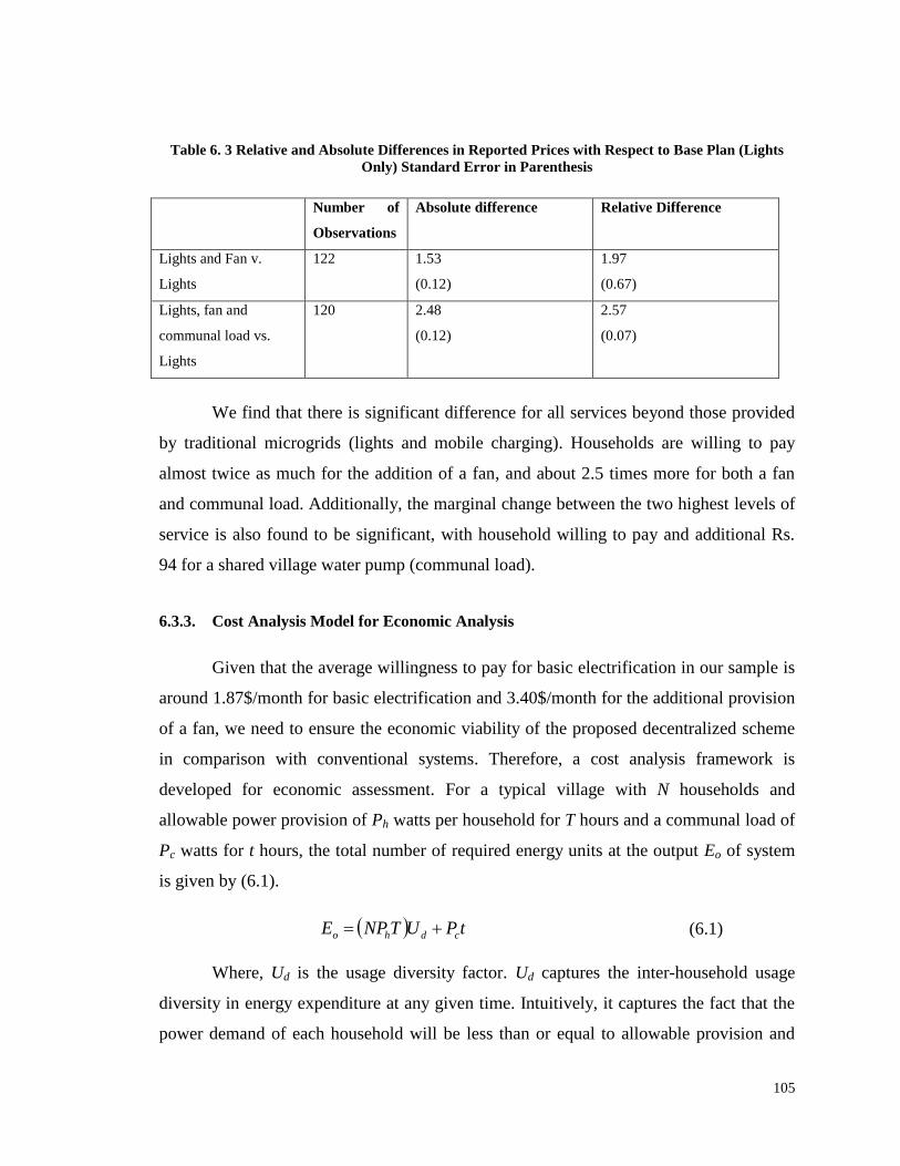
105

Table 6. 3 Relative and Absolute Differences in Reported Prices with Respect to Base Plan (Lights

Only) Standard Error in Parenthesis

Number of

Observations

Absolute difference Relative Difference

Lights and Fan v.

Lights

122 1.53

(0.12)

1.97

(0.67)

Lights, fan and

communal load vs.

Lights

120 2.48

(0.12)

2.57

(0.07)

We find that there is significant difference for all services beyond those provided

by traditional microgrids (lights and mobile charging). Households are willing to pay

almost twice as much for the addition of a fan, and about 2.5 times more for both a fan

and communal load. Additionally, the marginal change between the two highest levels of

service is also found to be significant, with household willing to pay and additional Rs.

94 for a shared village water pump (communal load).

6.3.3. Cost Analysis Model for Economic Analysis

Given that the average willingness to pay for basic electrification in our sample is

around 1.87$/month for basic electrification and 3.40$/month for the additional provision

of a fan, we need to ensure the economic viability of the proposed decentralized scheme

in comparison with conventional systems. Therefore, a cost analysis framework is

developed for economic assessment. For a typical village with N households and

allowable power provision of Ph watts per household for T hours and a communal load of

Pc watts for t hours, the total number of required energy units at the output Eo of system

is given by (6.1).

tPUTNPE cdho (6.1)

Where, Ud is the usage diversity factor. Ud captures the inter-household usage

diversity in energy expenditure at any given time. Intuitively, it captures the fact that the

power demand of each household will be less than or equal to allowable provision and

106

will be different from other households in the village. It is typically assumed that Ud < 1,

i.e. on average households are consuming below their allowed provision. For example, it

is reasonable to assume from a design perspective that in the day time when sunlight is

available, lighting load at each household will be reduced. Similarly, in winters the fan

loads will be reduced due to seasonal variation in temperature and associated cooling

requirements. Therefore, panel requirements are reduced accordingly and are quantified

in (6.1). The capability to extract the benefit of usage diversity is precisely the reason

microgrids are more efficient that standalone systems.

Given the energy requirement of a system, system characteristics such as solar PV

panel sizing required to produce the requisite amount of power must be calculated. These

must take into account the incident irradiance, effect of temperature degradation and

various losses including wiring losses, converter losses, and storage losses during

charging/discharging cycle losses. To account for various energy losses and degradation

in a system, the amount of energy needed to be produced, , is given by (6.2).

DCBT

P

EE

0

(6.2)

Where, and are degradation in efficiency due to temperature, storage

(or battery) inefficiency, converter inefficiency and line losses, respectively. The

resulting panel size needed at per household can be expressed by (6.3).

NE

EP

p

PV

(6.3)

Where, ̅ is the average value of peak sunlight hours for the particular region.

Similarly, for first order cost calculation model for a battery system, the battery energy

capacity is determined by the total energy that battery has to supply when the sun is

not available along with the extra energy that is dissipated during charging/discharging.

Moreover, to extend the battery life, generally there is a limit on minimum discharging

state (%), which again tends to increase the required battery capacity. The

overall battery requirement for a microgrid then is given by (6.4).

107

B

hB

N

SOCPEPSHE

min124

(6.4)

In addition to storage and solar panel costs, there are other costs which include the

cost of converters, system protection equipment and conductor (wiring) length. The price

of converters is generally proportional to their power processing requirements, loading

levels and current carrying capacity. Therefore, for simplicity, it can be taken as a fixed

percentage, , of the total cost of PV panel. Similarly, the cost of protection is

proportional to the power loading level and short circuit current capacity, therefore, in the

current analysis it can be taken as a fixed percentage as well ( ). Finally, the cost of

total conductor length ( ) is given by C3 (USD/m). Considering PV panel cost as C1

(USD/watt) and battery cost as C2 (USD/watt), total system upfront cost CU is given by

(6.5).

PBPVCU lCECPCC 11 321 (6.5)

Generally, life time of a solar panel is 25 years, while the life time of battery can be taken

as years and life time of power electronic converters is given by years. Therefore,

for a typical 25 year system, the operation and maintenance cost, along with the number

of battery and power converters replacement is calculated and added with the capital cost

to find the overall lifetime cost of the system. The total lifetime cost CLT of the system

over its lifetime is then given by (6.6).

PCPV

c

B

B

ULT PCN

ECN

CC

11

251

2512

(6.6)

Further, it is important to evaluate the effective levelized cost of electricity (LCOE)

(USD/kWh) of system, given by equation (6.7), which effectively calculates the cost of

each unit produced by the microgrid over its 25 year operation in comparison to the

lifecycle costs.

)25)(1000)(365(O

LT

E

CLCOE

(6.7)

108

As, Eo is the energy produced per day which is multiplied by 365 (days in a year) and 25

(operational lifetime of the system). 1000 (in the denominator) gives LCOE in price per

kWh as kWh is standard unit for electricity production/consumption. The presented cost

model is applied for the electrification of a typical village having 40 houses, 30W rated

power at each house with ± 100% flexibility in power provision i.e. each house may

consume up to 60W (double of its rated power) of electricity, or may sell 30W of

electricity at a given time. The rated power provisioning is in accordance with the market

availability of DC loads with three lighting bulbs (~4W each), one DC fan (~14 W) and

one mobile charging unit (~4 W). Similarly, for the village under analysis a communal

load of up to 500W is considered for water filtration plant/pump for drinking purposes.

The household operation is for 24 hours while communal load operation is considered for

6 hours per day. The value of average peak sunlight hours ̅ for the typical village is

assumed to be 6 hours per day, i.e. (6 hours of standard daylight on average over the

year).

6.3.4. Results of Economic Analysis

The proposed first-order cost analysis model is applied on the village with

specifications discussed above to calculate system sizing requirements and associated

costs. Usage diversity factor is considered 0.3, which approximates lack of simultaneous

loading for all households at all the time. The costs are taken as followings:

PV panel price =0.8 $/kWp [118, 119],

battery price =1.05$ $/Wh [111] (Lead acid battery),

distribution conductor cost for the village is $500 and converter cost factor =0.3

and protection cost factor = 0.05 [120].

Therefore, considering all these factors, LCOE, along with flat rate tariff plan for

the proposed and existing schemes of electrification is calculated over 25 year project

life. For 6 years ROI plan, one battery replacement is considered, for 9 years ROI plan,

one battery and one charge controller replacement is considered, while for 12 years ROI

plan 2 batteries and one charge controller replacement is considered. Table 6.4 presents

the estimated costs of all three levels of services including and compares them to

109

alternative implementations. Kindly note that these are typical costs and the prices may

vary from one region to another. There may well be additional costs for some newer

aspects of efficient power processing (power electronics) in distributed microgrids. Solar

panels, storage and distribution prices used are standard wholesaler‘s rates, correct for the

month of December 2017.

Calculations show that solar power, in particular decentralized microgrids, present

a viable alternative to grid electricity even for loads beyond high quality light. Load

sharing allows the system to even provide electricity for a communal load for a negligible

increase in price. A major component to the cost of any solar system is the cost of

storage. Batteries are both expensive, have short life spans and are inefficient. However,

recent developments in battery technology suggest that the overall cost of such a system

is likely to come down in future. As an example, for a case of a decentralized microgrid,

we show that the cost of storage highly dominates the overall cost of the system in its

lifespan of 25 years (figure 6.1), at current market prices.

Table 6. 4 Estimated Cost of decentralized Solar Generation Implementations through DGDSA

Scenario Load per house

(24/7 provision

to subscribers)

Capital

Cost

(USD)

Effective

LCOE

(USD)

Capital +

25 years

O&M Cost

(USD)

Subscription Charges Per user per

Month for payback in (USD/Month)

3 years 6

years

9

years

12

years

Traditional

microgrid

(e..g. MGP)

1 light + mobile

charging unit

(5W).

2117 0.11 4775 1.47 0.91 0.66 0.62

Decentralized

Microgrid

3 Lights,

1 fan, charging

unit

(30W)

9563 0.10 26149 6.65 4.45 3.30 2.70

3 Lights,

1 fan, charging

unit and

Communal load

(30W +500W)

10000 0.09 26787 6.95

4.73 3.50 3.25

Standalone

Production

and

Consumption

(No grid)

3 Lights,

1 fan, charging

unit

(30W)

10828 0.11 29300 7.50 5.15 3.50 3.30

3 Lights,

1 fan, charging

unit and

Communal load

(30W + 500W)

11658 0.11 31304 8.10 5.6 4.0 3.80

110

Figure 6. 1 Life Time Operation Cost Break-up of a Distributed Microgrid

From the highlights of economic analysis that distributed microgrid architecture

presented in this thesis has a potential to create a micro-energy economy with a viable,

scalable and profitable microgrid model providing opportunities for entrepreneurs to

enter the market and also provide new sources of employment.

6.4. Future work

Our findings indicate that distributed solar microgrids present a promising route

to rural electrification, especially in areas where grid expansion may be prohibitively

expensive. They have the capacity and scalability to provide electricity beyond those

offered by traditional microgrids. In countries like Pakistan, that are already facing major

crises in supply, they present a low cost solution to not just the distribution problem, but

also the problem of generation. The next steps in this agenda would be the roll out pilots

of distributed microgrids in the surveyed areas to evaluate the performance of the system

along with its uptake in various regions. Further, a natural area for expansion would be to

study the appropriateness of microgrids as a source of back up electricity in on grid areas,

experiencing high number of rolling black outs. Along with that following are the key

16%

57%

14%

4% 4%

5%

25 years Operation Cost of the Distributed Microgrid

PV Panel Cost

Battery Storage Cost

Controller+ Converter Cost

Conductors Cost

others

Protection Cost

111

area that needs to be researched for successful practical deployment of the proposed

distributed microgrids.

In order to enable energy trading among multiple nanogrids, there must be a

mechanism to monitor energy transactions among neighboring nanogrids.

Although energy trade mechanism will formulate a local energy market and will

be helpful for empowering rural inhabitants, however, it will require a

communication layer at neighborhood levels to ensure monitoring of energy

exchange.

A key challenge for the successful implementation of such a distributed system

will be the development of theft monitoring mechanism which will be based upon

remote monitoring and communication system to ensure provisioned power flow.

Since battery storage system is the prime cost element in such systems, therefore,

a mechanism must be incorporated for battery state of charge, depth of discharge

and state of health monitoring for the maximization of battery life and preventive

maintenance.

The proposed architecture must be robust; therefore, a distributed, yet coordinated

and selective protection scheme must be developed to ensure the reliability of the

system as well as longevity of the power electronic equipment.

A scheme for optimal dispatch of the distributed resources based upon time

varying household and communal load requirements needs to be developed for

efficient resource utilization.

112

Bibliography

[1] World Energy Outlook (WEO, 2017), Electricity Access Database [Online].

Available:

https://www.iea.org/publications/freepublications/publication/WEO2017SpecialR

eport_EnergyAccessOutlook.pdf

[2] M. Lavelle. (2012, Cookstove Smoke is ―Largest Environmental Threat,‖.

Available: http://energyblog.nationalgeographic.com/2012/12/13/cookstove-

smoke-is-largest-environmental-threat-global-health-study-finds/

[3] N. L. Lam, K. R. Smith, A. Gauthier, and M. N. Bates, "Kerosene: a review of

household uses and their hazards in low-and middle-income countries," Journal of

Toxicology and Environmental Health, Part B, vol. 15, pp. 396-432, 2012.

[4] J. Peters and M. Sievert, "Impacts of rural electrification revisited–the African

context," Journal of Development Effectiveness, vol. 8, pp. 327-345, 2016.

[5] K. Reiche, A. Covarrubias, and E. Martinot, "Expanding electricity access to

remote areas: off-grid rural electrification in developing countries," Fuel, vol. 1,

p. 1.4, 2000.

[6] A. M. Tanner and A. L. Johnston, "The Impact of Rural Electric Access on

Deforestation Rates," World Development, vol. 94, pp. 174-185, 2017.

[7] F. Yang and M. Yang, "Rural electrification in sub-Saharan Africa with

innovative energy policy and new financing models," Mitigation and Adaptation

Strategies for Global Change, pp. 1-20, 2017.

[8] J. Chi, W. Peng, X. Jianfang, T. Yi, and C. Fook Hoong, "Implementation of

Hierarchical Control in DC Microgrids," Industrial Electronics, IEEE

Transactions on, vol. 61, pp. 4032-4042, 2014.

[9] World Energy Outlook (WEO, 2016), Electricity Access Database [Online].

Available:

http://www.worldenergyoutlook.org/resources/energydevelopment/energyaccessd

atabase/.

[10] G. He and D. G. Victor, "Experiences and lessons from China‘s success in

providing electricity for all," Resources, Conservation and Recycling, vol. 122,

pp. 335-338, 2017.

[11] Rajendra Singh and K. Shenai. (2014, DC Microgrids and the Virtues of Local

Electricity. IEEE Spectrum. Available: http://spectrum.ieee.org/green-

http://www.iea.org/publications/freepublications/publication/WEO2017SpecialReport_EnergyAccessOutlook.pdf

http://www.iea.org/publications/freepublications/publication/WEO2017SpecialReport_EnergyAccessOutlook.pdf

http://energyblog.nationalgeographic.com/2012/12/13/cookstove-smoke-is-largest-environmental-threat-global-health-study-finds/

http://energyblog.nationalgeographic.com/2012/12/13/cookstove-smoke-is-largest-environmental-threat-global-health-study-finds/

http://www.worldenergyoutlook.org/resources/energydevelopment/energyaccessdatabase/

http://www.worldenergyoutlook.org/resources/energydevelopment/energyaccessdatabase/

http://spectrum.ieee.org/green-tech/buildings/dc-microgrids-and-the-virtues-of-local-electricity/?utm_source=energywise&utm_medium=email&utm_campaign=021214

113

tech/buildings/dc-microgrids-and-the-virtues-of-local-

electricity/?utm_source=energywise&utm_medium=email&utm_campaign=0212

14

[12] P. Brinckerhoff, "Electricity Transmission Costing Study," IET, 2012.

[13] M. Nasir and A. A. Bhatti, "A Micro Computer-Based Methodology for Distance

Protection on Long UHV Transmission Lines Using Symmetrical Components,"

in Power and Energy Engineering Conference (APPEEC), 2012 Asia-Pacific,

2012, pp. 1-6.

[14] M. N. Qaiser, M. Usama, B. Ahmad, M. A. Tariq, and H. A. Khan, "Low Cost,

Robust and Efficient Implementation of MPPT based Buck-Boost Converter for

Off-grid PV Applications," presented at the 40th IEEE Photovoltaic Specialists

Conference, Denver Colorado, USA, 2014.

[15] H. A. Khan and S. Pervaiz, "Technological review on solar PV in Pakistan:

Scope, practices and recommendations for optimized system design," Renewable

and Sustainable Energy Reviews, vol. 23, pp. 147-154, 2013.

[16] S. R. Khandker, H. A. Samad, Z. K. Sadeque, M. Asaduzzaman, M. Yunus, and

A. E. Haque, Surge in solar-powered homes: Experience in off-grid rural

Bangladesh: World Bank Publications, 2014.

[17] Solar Home System programme by Infrastucture Development Company

(IDCOL), Bangladesh [Online]. Available: http://idcol.org/home/solar

[18] I. Khan, Y. Xu, H. Sun, and V. Bhattacharjee, "Distributed Optimal Reactive

Power Control of Power Systems," IEEE Access, vol. 6, pp. 7100-7111, 2018.

[19] D. Schnitzer, D. S. Lounsbury, J. P. Carvallo, R. Deshmukh, J. Apt, and D. M.

Kammen, "Microgrids for Rural Electrification: A critical review of best practices

based on seven case studies," United Nations Foundation, 2014.

[20] D. Palit and G. K. Sarangi, "Renewable energy based mini-grids for enhancing

electricity access: Experiences and lessons from India," in International

Conference and Utility Exhibition on Green Energy for Sustainable Development

(ICUE),\ 19-21 March 2014, pp. 1-8.

[21] J. Urpelainen, "Energy poverty and perceptions of solar power in marginalized

communities: Survey evidence from Uttar Pradesh, India," Renewable Energy,

vol. 85, pp. 534-539, 2016.

[22] S. Mishra and O. Ray, "Advances in nanogrid technology and its integration into

rural electrification in India," in Power Electronics Conference (IPEC-Hiroshima

2014-ECCE-ASIA), 2014 International, 2014, pp. 2707-2713.




http://idcol.org/home/solar

114

[23] D. Palit, G. K. Sarangi, and P. Krithika, "Energising Rural India Using

Distributed Generation: The Case of Solar Mini-Grids in Chhattisgarh State,

India," in Mini-Grids for Rural Electrification of Developing Countries, ed:

Springer, 2014, pp. 313-342.

[24] S. Chakrabarti and S. Chakrabarti, "Rural electrification programme with solar

energy in remote region–a case study in an island," Energy Policy, vol. 30, pp. 33-

42, 2002.

[25] H. Jiayi, J. Chuanwen, and X. Rong, "A review on distributed energy resources

and MicroGrid," Renewable and Sustainable Energy Reviews, vol. 12, pp. 2472-

2483, 12// 2008.

[26] R. H. Lasseter, "MicroGrids," in Power Engineering Society Winter Meeting,

2002. IEEE, 2002, pp. 305-308 vol.1.

[27] N. Hatziargyriou, H. Asano, R. Iravani, and C. Marnay, "Microgrids," Power and

Energy Magazine, IEEE, vol. 5, pp. 78-94, 2007.

[28] B. S. Hartono, Y. Budiyanto, and R. Setiabudy, "Review of microgrid

technology," in QiR (Quality in Research), 2013 International Conference on, pp.

127-132.

[29] R. H. Lasseter and P. Paigi, "Microgrid: a conceptual solution," in Power

Electronics Specialists Conference, 2004. PESC 04. 2004 IEEE 35th Annual,

2004, pp. 4285-4290 Vol.6.

[30] M. Soshinskaya, W. H. Crijns-Graus, J. M. Guerrero, and J. C. Vasquez,

"Microgrids: Experiences, barriers and success factors," Renewable and

Sustainable Energy Reviews, vol. 40, pp. 659-672, 2014.

[31] J. B. Almada, R. P. S. Leao, F. F. D. Montenegro, S. S. V. Miranda, and R. F.

Sampaio, "Modeling and simulation of a microgrid with multiple energy

resources," in EUROCON, 2013 IEEE, 2013, pp. 1150-1157.

[32] L. Xuan and S. Bin, "Microgrids — an integration of renewable energy

technologies," in Electricity Distribution, 2008. CICED 2008. China

International Conference on, 2008, pp. 1-7.

[33] A. S. Rana, M. Nasir, and H. A. Khan, "String level optimisation on grid-tied

solar PV systems to reduce partial shading loss," IET Renewable Power

Generation, 2017.

[34] M. Nasir, A. A. Bhatti, and W. T. Toor, "Model formulation and design of an

efficient control algorithm for fuel cell power system," in Power Engineering,

115

Energy and Electrical Drives (POWERENG), 2013 Fourth International

Conference on, 2013, pp. 806-811.

[35] M. Nasir and H. A. Khan, "Solar photovoltaic integrated building scale hybrid

AC/DC microgrid," 2016.

[36] K. Siraj, H. Siraj, and M. Nasir, "Modeling and control of a doubly fed induction

generator for grid integrated wind turbine," in Power Electronics and Motion

Control Conference and Exposition (PEMC), 2014 16th International, 2014, pp.

901-906.

[37] F. Zia, M. Nasir, and A. A. Bhatti, "Optimization methods for constrained

stochastic wind power economic dispatch," in Power Engineering and

Optimization Conference (PEOCO), 2013 IEEE 7th International, 2013, pp. 129-

133.

[38] J. Peters and M. Sievert, "Impacts of rural electrification revisited: The African

context," Ruhr Economic Papers 3867886377, 2015.

[39] N. Sasidharan, J. G. Singh, and W. Ongsakul, "An approach for an efficient

hybrid AC/DC solar powered Homegrid system based on the load characteristics

of home appliances," Energy and Buildings, vol. 108, pp. 23-35, 2015.

[40] N. Bashir, H. S. Sardar, M. Nasir, N. U. Hassan, and H. A. Khan, "Lifetime

maximization of lead-acid batteries in small scale UPS and distributed generation

systems," in PowerTech, 2017 IEEE Manchester, 2017, pp. 1-6.

[41] F. Dastgeer and A. Kalam, "Efficiency comparison of DC and AC distribution

systems for distributed generation," in Power Engineering Conference, 2009.

AUPEC 2009. Australasian Universities, 2009, pp. 1-5.

[42] J. J. Justo, F. Mwasilu, J. Lee, and J.-W. Jung, "AC-microgrids versus DC-

microgrids with distributed energy resources: A review," Renewable and

Sustainable Energy Reviews, vol. 24, pp. 387-405, 2013.

[43] H. E. Gelani, M. Nasir, F. Dastgeer, and H. Hussain, "Efficiency Comparison of

Alternating Current (AC) and Direct Current (DC) Distribution System at

Residential Level with Load Characterization and Daily Load Variation."

[44] P. A. Madduri, J. Rosa, S. R. Sanders, E. Brewer, and M. Podolsky, "Design and

verification of smart and scalable DC microgrids for emerging regions," in

Energy Conversion Congress and Exposition (ECCE), 2013 IEEE, 2013, pp. 73-

79.

[45] D. J. Hammerstrom, "AC versus DC distribution systemsdid we get it right?," in

Power Engineering Society General Meeting, 2007. IEEE, 2007, pp. 1-5.

116

[46] D. Nilsson and A. Sannino, "Efficiency analysis of low-and medium-voltage DC

distribution systems," in Power Engineering Society General Meeting, 2004.

IEEE, 2004, pp. 2315-2321.

[47] H. Kakigano, Y. Miura, and T. Ise, "Low-Voltage Bipolar-Type DC Microgrid for

Super High Quality Distribution," Power Electronics, IEEE Transactions on, vol.

25, pp. 3066-3075, 2010.

[48] D. Soto and V. Modi, "Simulations of Efficiency Improvements Using Measured

Microgrid Data," in Global Humanitarian Technology Conference (GHTC), 2012

IEEE, 2012, pp. 369-374.

[49] W. A. Simon Willems, Stijn De Jonge, Dries Haeseldonckx, Pepijn van

Willigenburg, Johan Woudstra and Harry Stokman, "Sustainable Impact and

Standardization of a DC Micro Grid," ed. ‖ Proceedings of Ecodesign 2013

International Symposium, 2013-12-06.

[50] D. J. Becker and B. J. Sonnenberg, "DC microgrids in buildings and data centers,"

in Telecommunications Energy Conference (INTELEC), 2011 IEEE 33rd

International, 2011, pp. 1-7.

[51] (2001, Table US-1. Electricity consumption by end use in U.S. households, 2001,

Energy Information Administration

[52] A. C. Brent and D. E. Rogers, "Renewable rural electrification: Sustainability

assessment of mini-hybrid off-grid technological systems in the African context,"

Renewable Energy, vol. 35, pp. 257-265, 2010.

[53] J. W. Stevens and G. P. Corey, "A study of lead-acid battery efficiency near top-

of-charge and the impact on PV system design," in Photovoltaic Specialists

Conference, 1996., Conference Record of the Twenty Fifth IEEE, 1996, pp. 1485-

1488.

[54] P. A. Madduri, J. Rosa, S. R. Sanders, E. A. Brewer, and M. Podolsky, "Design

and verification of smart and scalable DC microgrids for emerging regions," in

Energy Conversion Congress and Exposition (ECCE), 2013 IEEE, 2013, pp. 73-

79.

[55] S. B. Tennakoon and P. M. McEwan, "Short-circuit interruption performance of

thyristor circuit breakers," in Applied Power Electronics Conference and

Exposition, 1994. APEC '94. Conference Proceedings 1994., Ninth Annual, 1994,

pp. 832-838 vol.2.

117

[56] M. E. Baran and N. R. Mahajan, "Overcurrent Protection on Voltage-Source-

Converter-Based Multiterminal DC Distribution Systems," Power Delivery, IEEE

Transactions on, vol. 22, pp. 406-412, 2007.

[57] M. Wang, M. Abedrabbo, W. Leterme, D. Van Hertem, C. Spallarossa, S.

Oukaili, I. Grammatikos, and K. Kuroda, "A Review on AC and DC Protection

Equipment and Technologies: Towards Multivendor Solution," 2017.

[58] A. Mohamed, V. Salehi, and O. Mohammed, "Real-Time Energy Management

Algorithm for Mitigation of Pulse Loads in Hybrid Microgrids," Smart Grid,

IEEE Transactions on, vol. 3, pp. 1911-1922, 2012.

[59] H. Kakigano, M. Nomura, and T. Ise, "Loss evaluation of DC distribution for

residential houses compared with AC system," in Power Electronics Conference

(IPEC), 2010 International, 2010, pp. 480-486.

[60] D. Salomonsson, L. Soder, and A. Sannino, "Protection of Low-Voltage DC

Microgrids," Power Delivery, IEEE Transactions on, vol. 24, pp. 1045-1053,

2009.

[61] A. R. Mohammad Ali Tavakkoli, Houshang Hassibi, "Simulation and Analysis of

a Compact Electronic Infrastructure for DC Micro-Grid: Necessity and

Challenges," Smart Grid and Renewable Energy, vol. Vol.3 pp. pp. 73-82., May

2012.

[62] A. K. Srivastava, "Solar minigrids in rural areas of Uttar Pradesh," Akshay Urja,

vol. 4, pp. 16-17, 2013.

[63] F. Pearce. World's poor need grid power, not just solar panels. Energy and Fuels

2980, 2014.

[64] P. A. Madduri, J. Poon, J. Rosa, M. Podolsky, E. Brewer, and S. R. Sanders,

"Scalable DC Microgrids for Rural Electrification in Emerging Regions," IEEE

Journal of Emerging and Selected Topics in Power Electronics, vol. PP, pp. 1-1,

2016.

[65] W. Inam, D. Strawser, K. K. Afridi, R. J. Ram, and D. J. Perreault, "Architecture

and system analysis of microgrids with peer-to-peer electricity sharing to create a

marketplace which enables energy access," in Power Electronics and ECCE Asia

(ICPE-ECCE Asia), 2015 9th International Conference on, 2015, pp. 464-469.

[66] T. Dragičević, J. M. Guerrero, J. C. Vasquez, and D. Škrlec, "Supervisory control

of an adaptive-droop regulated DC microgrid with battery management

capability," IEEE Transactions on Power Electronics, vol. 29, pp. 695-706, 2014.

118

[67] Q. Shafiee, T. Dragičević, J. C. Vasquez, and J. M. Guerrero, "Hierarchical

control for multiple DC-microgrids clusters," IEEE Transactions on Energy

Conversion, vol. 29, pp. 922-933, 2014.

[68] J. M. Guerrero, J. C. Vasquez, J. Matas, L. G. De Vicuña, and M. Castilla,

"Hierarchical control of droop-controlled AC and DC microgrids—A general

approach toward standardization," IEEE Transactions on Industrial Electronics,

vol. 58, pp. 158-172, 2011.

[69] I. Khan, Y. Xu, S. Kar, and H. Sun, "Compressive Sensing-Based Optimal

Reactive Power Control of a Multi-Area Power System," IEEE Access, vol. 5, pp.

23576-23588, 2017.

[70] I. Khan, Z. Li, Y. Xu, and W. Gu, "Distributed control algorithm for optimal

reactive power control in power grids," International Journal of Electrical Power

& Energy Systems, vol. 83, pp. 505-513, 2016.

[71] M. Nasir, H. A. Khan, A. Hussain, L. Mateen, and N. A. Zaffar, "Solar PV-Based

Scalable DC Microgrid for Rural Electrification in Developing Regions," IEEE

Transactions on Sustainable Energy, vol. 9, pp. 390-399, 2018.

[72] C. S. Solanki, Solar photovoltaics: fundamentals, technologies and applications:

PHI Learning Pvt. Ltd., 2011.

[73] B. Subudhi and R. Pradhan, "A comparative study on maximum power point

tracking techniques for photovoltaic power systems," Sustainable Energy, IEEE

transactions on, vol. 4, pp. 89-98, 2013.

[74] M. Nasir and M. F. Zia, "Global maximum power point tracking algorithm for

photovoltaic systems under partial shading conditions," in Power Electronics and

Motion Control Conference and Exposition (PEMC), 2014 16th International,

2014, pp. 667-672.

[75] R. W. Erickson and D. Maksimovic, Fundamentals of power electronics: Springer

Science & Business Media, 2007.

[76] R. Pasonen, "Model of Bi-directional Flyback Converter for Hybrid AC/DC

Distribution System," International Journal of Power Electronics and Drive

Systems (IJPEDS), vol. 3, pp. 444-449, 2013.

[77] H. Saadat, Power system analysis: WCB/McGraw-Hill, 1999.

[78] V. Mehta and R. Mehta, Principles of power system: S. Chand, 1982.

119

[79] M. Nasir, N. A. Zaffar, and H. A. Khan, "Analysis on central and distributed

architectures of solar powered DC microgrids," in 2016 Clemson University

Power Systems Conference (PSC), 2016, pp. 1-6.

[80] B. Stott and O. Alsaç, "Fast decoupled load flow," power apparatus and systems,

ieee transactions on, pp. 859-869, 1974.

[81] G.-X. Luo and A. Semlyen, "Efficient load flow for large weakly meshed

networks," Power Systems, IEEE Transactions on, vol. 5, pp. 1309-1316, 1990.

[82] R. Farooq, L. Mateen, M. Ahmad, S. Q. Akbar, H. A. Khan, and N. A. Zaffar,

"Smart DC microgrids: Modeling and power flow analysis of a DC Microgrid for

off-grid and weak-grid connected communities," in Power and Energy

Engineering Conference (APPEEC), 2014 IEEE PES Asia-Pacific, 2014, pp. 1-6.

[83] S. Anand and B. Fernandes, "Optimal voltage level for DC microgrids," in

IECON 2010-36th Annual Conference on IEEE Industrial Electronics Society,

2010, pp. 3034-3039.

[84] M. J. Sarker, B. Asare-Bediako, J. Slootweg, W. Kling, and B. Alipuria, "DC

micro-grid with distributed generation for rural electrification," in Universities

Power Engineering Conference (UPEC), 2012 47th International, 2012, pp. 1-6.

[85] A. Sannino, G. Postiglione, and M. H. Bollen, "Feasibility of a DC network for

commercial facilities," Industry Applications, IEEE Transactions on, vol. 39, pp.

1499-1507, 2003.

[86] K. Engelen, E. L. Shun, P. Vermeyen, I. Pardon, R. D'hulst, J. Driesen, and R.

Belmans, "The feasibility of small-scale residential DC distribution systems," in

IEEE Industrial Electronics, IECON 2006-32nd Annual Conference on, 2006, pp.

2618-2623.

[87] A. Pratt, P. Kumar, and T. V. Aldridge, "Evaluation of 400V DC distribution in

telco and data centers to improve energy efficiency," in Telecommunications

Energy Conference, 2007. INTELEC 2007. 29th International, 2007, pp. 32-39.

[88] K. R. Varshney, G. H. Chen, B. Abelson, K. Nowocin, V. Sakhrani, L. Xu, and B.

L. Spatocco, "Targeting villages for rural development using satellite image

analysis," Big Data, vol. 3, pp. 41-53, 2015.

[89] B. Patterson, "LVDC: from concept to practice: an EMerge perspective," 2015.

[90] D. Salomonsson, L. Soder, and A. Sannino, "Protection of low-voltage DC

microgrids," IEEE Transactions on Power Delivery, vol. 24, pp. 1045-1053,

2009.

120

[91] N. F. P. Association, NFPA 70: National Electrical Code:

NationalFireProtectionAssoc, 2011.

[92] I. Marx, "Combining the best of both worlds," Industry Applications Magazine,

IEEE, vol. 16, pp. 30-34, 2010.

[93] A. F. X. Welsch, "DC Installation, Different Hazards Regarding Thermal Effects

and Electrical Shock," IEC LVDC Workshop, University of Applied Science,

Regensburg, 2011.

[94] X. Lu, K. Sun, J. M. Guerrero, J. C. Vasquez, and L. Huang, "State-of-charge

balance using adaptive droop control for distributed energy storage systems in DC

microgrid applications," IEEE Transactions on Industrial Electronics, vol. 61, pp.

2804-2815, 2014.

[95] Z. Jin, L. Meng, and J. M. Guerrero, "Comparative admittance-based analysis for

different droop control approaches in DC microgrids," in DC Microgrids

(ICDCM), 2017 IEEE Second International Conference on, 2017, pp. 515-522.

[96] M. Nasir, S. Iqbal, and H. A. Khan, "Optimal Planning and Design of Low-

Voltage Low-Power Solar DC Microgrids," IEEE Transactions on Power

Systems, vol. 33, pp. 2919-2928, 2018.

[97] M. Nasir, Z. Jin, H. Khan, N. Zaffar, J. Vasquez, and J. M. Guerrero, "A

Decentralized Control Architecture applied to DC Nanogrid Clusters for Rural

Electrification in Developing Regions," IEEE Transactions on Power Electronics,

2018.

[98] L. Meng, M. Savaghebi, F. Andrade, J. C. Vasquez, J. M. Guerrero, and M.

Graells, "Microgrid central controller development and hierarchical control

implementation in the intelligent microgrid lab of Aalborg University," in Applied

Power Electronics Conference and Exposition (APEC), 2015 IEEE, 2015, pp.

2585-2592.

[99] M. Hamza, M. Shehroz, S. Fazal, M. Nasir, and H. A. Khan, "Design and analysis

of solar PV based low-power low-voltage DC microgrid architectures for rural

electrification," in Power & Energy Society General Meeting, 2017 IEEE, 2017,

pp. 1-5.

[100] A. R. Desai, Rural sociology in India: Popular Prakashan, 1994.

[101] T. Odeyale and T. Adekunle, "Innovative and sustainable local material in

traditional African architecture–Socio cultural dimension," 2008.

121

[102] C. Linard, M. Gilbert, R. W. Snow, A. M. Noor, and A. J. Tatem, "Population

distribution, settlement patterns and accessibility across Africa in 2010," PloS

one, vol. 7, p. e31743, 2012.

[103] M. Silberfein, Rural settlement structure and African development: Westview

Press, 1998.

[104] S. C. Bhattacharyya and D. Palit, "Mini-grid based off-grid electrification to

enhance electricity access in developing countries: What policies may be

required?," Energy Policy, vol. 94, pp. 166-178, 2016.

[105] M. M. H. Sajeeb, A. Rahman, and S. Arif, "Feasibility analysis of solar DC Nano

grid for off grid rural Bangladesh," in Green Energy and Technology (ICGET),

2015 3rd International Conference on, 2015, pp. 1-5.

[106] S. Pervaiz and H. A. Khan, "Low irradiance loss quantification in c-Si panels for

photovoltaic systems," Journal of Renewable and Sustainable Energy, vol. 7, p.

013129, 2015.

[107] M. R. Maghami, H. Hizam, C. Gomes, M. A. Radzi, M. I. Rezadad, and S.

Hajighorbani, "Power loss due to soiling on solar panel: A review," Renewable

and Sustainable Energy Reviews, vol. 59, pp. 1307-1316, 2016.

[108] E. Forniés, F. Naranjo, M. Mazo, and F. Ruiz, "The influence of mismatch of

solar cells on relative power loss of photovoltaic modules," Solar Energy, vol. 97,

pp. 39-47, 2013.

[109] C. S. Solanki, Solar photovoltaics: fundamentals, technologies and applications:

PHI Learning Pvt. Ltd., 2015.

[110] J. Kolar, F. Krismer, Y. Lobsiger, J. Muhlethaler, T. Nussbaumer, and J.

Minibock, "Extreme efficiency power electronics," in Integrated Power

Electronics Systems (CIPS), 2012 7th International Conference on, 2012, pp. 1-

22.

[111] S. Matteson and E. Williams, "Residual learning rates in lead-acid batteries:

Effects on emerging technologies," Energy Policy, vol. 85, pp. 71-79, 2015/10/01/

2015.

[112] S. M. Schoenung and W. V. Hassenzahl, "Long-vs. short-term energy storage

technologies analysis: a life-cycle cost study: a study for the DOE energy storage

systems program," Sandia National Laboratories2003.

[113] M. Nasir, S. Iqbal, and H. A. Khan, "Optimal Planning and Design of Low-

Voltage Low-Power Solar DC Microgrids," IEEE Transactions on Power

Systems, 2017.

122

[114] S. C. Bhattacharyya, "Financing energy access and off-grid electrification: A

review of status, options and challenges," Renewable and Sustainable Energy

Reviews, vol. 20, pp. 462-472, 2013.

[115] N. J. Williams, P. Jaramillo, J. Taneja, and T. S. Ustun, "Enabling private sector

investment in microgrid-based rural electrification in developing countries: A

review," Renewable and Sustainable Energy Reviews, vol. 52, pp. 1268-1281,

2015.

[116] D. Palit, "Solar energy programs for rural electrification: Experiences and lessons

from South Asia," Energy for Sustainable Development, vol. 17, pp. 270-279,

2013.

[117] A. Newcombe and E. K. Ackom, "Sustainable solar home systems model:

Applying lessons from Bangladesh to Myanmar's rural poor," Energy for

Sustainable Development, vol. 38, pp. 21-33, 2017.

[118] Q. Bao, T. Honda, S. El Ferik, M. M. Shaukat, and M. C. Yang, "Understanding

the role of visual appeal in consumer preference for residential solar panels,"

Renewable Energy, vol. 113, pp. 1569-1579, 2017/12/01/ 2017.

[119] J. Palm, "Household installation of solar panels – Motives and barriers in a 10-

year perspective," Energy Policy, vol. 113, pp. 1-8, 2018/02/01/ 2018.

[120] K. A. W. Horowitz, R. Fu, T. Silverman, M. Woodhouse, X. Sun, and M. A.

Alam, "An Analysis of the Cost and Performance of Photovoltaic Systems as a

Function of Module Area,"; National Renewable Energy Lab. (NREL), Golden,

CO (United States) NREL/TP-6A20-67006 United States 10.2172/1351153

NREL English, 2017.

scalable dc microgrids for rural electrification

Documents