h repetitive control of dc-ac converters in microgrids - spiral

IEEE TRANSACTIONS ON POWER ELECTRONICS, VOL. 19, NO. 1, JANUARY 2004 219

H Repetitive Control of DC-AC Convertersin Microgrids

George Weiss, Qing-Chang Zhong, Tim C. Green, Senior Member, IEEE, and Jun Liang, Member, IEEE

Abstract—This paper proposes a voltage controller designmethod for dc–ac converters supplying power to a microgrid,which is also connected to the power grid. This converter is meantto operate in conjunction with a small power generating unit.The design of the output voltage controller is based on andrepetitive control techniques. This leads to a very low harmonicdistortion of the output voltage, even in the presence of nonlinearloads and/or grid distortions. The output voltage controllercontains an infinite-dimensional internal model, which enables itto reject all periodic disturbances which have the same period asthe grid voltage, and whose highest frequency components are upto approximately 1.5 kHz.

Index Terms—DC–AC power converter, control, microgrid,repetitive control, total harmonic distortion (THD), voltage con-trol.

I. INTRODUCTION

FOR ECONOMIC, technical and environmental reasons,there is today a trend toward the use of small power gen-

erating units connected to the low-voltage distribution systemin addition to the traditional large generators connected to thehigh-voltage transmission system [1]. Not only is there a changeof scale but also a change of technology. Large generators arealmost exclusively 50/60 Hz synchronous machines. Distributedpower generators include variable speed (variable frequency)sources, high speed (high frequency) sources and direct energyconversion sources that produce dc. For example, wind-turbinesare most effective if free to generate at variable frequency and sothey require conversion from ac (variable frequency) to dc to ac(50/60 Hz) [2]; small gas-turbines with direct drive generatorsoperate at high frequency and also require ac to dc to ac conver-sion [3]; photo-voltaic arrays require dc–ac conversion [4]. In allof these cases the same basic inverter (dc to ac converter) will beused and needs to be controlled to provide high-quality supplywaveforms to consumers.

There are several operating regimes possible for distributedgeneration. One such is the microgrid in which the intention isthat local consumers are largely supplied by local generationbut that shortfalls or surpluses are exchanged through a connec-tion to the public electricity supply system [5], [6]. The use ofa microgrid opens up the possibility of making the distributed

Manuscript received January 12, 2003; revised July 16, 2003. This paper waspresented in part at the IEEE Conference on Decision and Control, Las Vegas,NV, December 10–13, 2002. This work was supported by EPSRC under Port-folio Partnership Grant GR/S61256/01. Recommended by Associate Editor B.Lehman.

The authors are with the Department of Electrical and Electronic Engineering,Imperial College London, London SW7 2BT, U.K. (e-mail: [email protected]).

Digital Object Identifier 10.1109/TPEL.2003.820561

Fig. 1. Single-phase representation of the system to be controlled. Thelocal loads are represented by a single linear load in parallel with aharmonic distortion current source. The PWM block is designed such that ifju(t)j < V =2 (no saturation), then the average of u over a switchingperiod is the control input u.

generator responsible for local power quality in a way that is notpossible with conventional generators [7].

Many of the loads connected to a distribution system ormicrogrid are nonlinear and create harmonically distorted cur-rent. The most common example is a linear load in serieswith a diode and with a dc-side capacitor. Many of the loadsare also single-phase and so considerable zero-sequence andnegative-sequence current components are expected. Becausethe grid has relatively high impedance at harmonic frequen-cies, the current distortion results in voltage distortion on thesupply to adjacent customers. Allowing the converter in agenerating unit to control the voltage of the microgrid willallow better power quality to be achieved. Fig. 1 shows thesystem to be controlled. The microgrid loads contain bothlinear and distorting elements. In Fig. 1, the loads have beenlumped together into one linear load and a current sink whichgenerates the harmonic components of the load current. Theconverter consists of a four-wire, three-phase inverter (IGBTbridge), an LC filter (to attenuate the switching frequencyvoltage components) and the controller. The microgrid canbe supplied solely by the local generator, or solely by thegrid, or by both in combination, or the local generator canboth supply the microgrid and export power. Two isolators,

and are provided to facilitate this and a grid interfaceinductor is provided to allow separation of the (sinusoidal)microgrid voltage and the (possibly distorted) grid voltageand also to facilitate the control of the real and reactive powerexchange between the microgrid and the grid.

There are several aspects to the control of such a system.1) DC-link balancing [8], [9]: to provide a neutral line, on

which the voltage is balanced w.r.t. the two terminals ofthe dc link, even when the three-phase system is not bal-anced and there is a large zero-sequence current compo-

0885-8993/04$20.00 © 2004 IEEE

220 IEEE TRANSACTIONS ON POWER ELECTRONICS, VOL. 19, NO. 1, JANUARY 2004

TABLE IPARAMETERS OF THE SYSTEM

nent. A balanced dc link enables the voltage control ofthe three-phase converter to be decoupled into the voltagecontrol of three single-phase converters.

2) Microgrid voltage control: to maintain a clean andbalanced microgrid voltage in the presence of nonlinearloads and/or grid distortions. A small THD is a majorobjective of the voltage controller.

3) Power control: to regulate the (active and reactive) powerexchange between the microgrid and the grid by gen-erating a suitable reference voltage for the voltage con-troller [10].

4) Connection, disconnection and protection of the micro-grid [11].

5) Discrete-time implementation of the controller using adigital signal processor.

This paper concentrates on one of these items only: microgridvoltage control. It is assumed that an outer control loop regu-lates the power exchange between the microgrid and the gridby developing appropriate reference voltages in terms of mag-nitude and phase shift with respect to the grid. These referencevoltages for the three phases of the microgrid voltage are sinu-soidal. It is then the task of the voltage controller to track ac-curately these reference voltages (so that the resulting THD issmall). This controller will be subject to disturbances which in-clude nonsinusoidal currents, changes in load current, changesand distortions in the grid voltage, and changes in the dc-linkvoltage.

Several control options exist. Conventional PI regulators canbe used and have been widely reported in inverter control. Ina rotating (dq) reference frame these regulators will seek tokeep the dq voltage components at their dc reference valuesand suppress distortion that appears as higher frequency terms.These controllers can work well on balanced systems, butare not good at correcting unbalanced disturbance currentswhich are a common feature of distribution systems (and thusare not good at controlling single-phase converters). Suchcontrollers are commonly employed for balanced three-phasemotor loads. Regulators in a stationary reference frame canoperate on a phase-by-phase basis and will have reasonablesuccess at maintaining balanced voltages. The difficulty comesin designing a regulator with the correct gain against frequencycharacteristic to regulate the fundamental frequency and rejecthigher harmonic disturbances. PI regulators with their pole(infinite gain) at zero-frequency are not best suited to this task.

A controller is required that has high gain at the fundamentaland all harmonic frequencies of interest. Repetitive control[12]–[15] is such a control technique. In this paper, we designthe voltage controller based on the repetitive control theorydeveloped in [12], leading to a very low harmonic distortion ofthe microgrid voltage even in the presence of nonlinear loadsand/or grid distortions.

II. SYSTEM MODELING

The three-phase power system consists of the converter (in-cluding the IGBT bridge and LC filters), the local consumers,the grid interface inductor and the (external) power grid. Dueto the presence of a balanced dc link (see [8], [9]), we may re-gard this system as three independent single-phase systems, asshown in Fig. 1, and hence there is no need to study here thethree-phase behavior of the system. This assumption may be in-accurate, with coupling between the phases present in some con-sumers, but this coupling will not have any significant influenceon the controller [10]. The filter inductor and other inductors inthe system include two parasitic resistances: a series resistor tomodel winding resistance and a parallel resistor to model corelosses. The resistance values we found from curve fitting ex-perimental impedance data over the frequency range 50 Hz to2 kHz.

The pulse-width-modulation (PWM) block is designed suchthat for , the local average of the bridge outputvoltage equals . This makes it possible to model the PWMblock and the inverter with an average voltage approach. ThePWM and inverter model is thus a simple saturated unity gain,where the saturation models the limit of the available dc-linkvoltage with respect to the neutral line . The nominalactive power in one phase of the load is 10 kW.

Our control objective is to maintain the microgrid voltageas close as possible to the given sinusoidal reference

voltage , so that the THD of is small. The two isolatorsand appearing in Fig. 1 are needed in the start-up and

shut-down procedures of the converter, which will not bediscussed in this paper, but some of it is discussed in [10].In this paper, the switches are considered to be closed. Theparameters of the system are shown in Table I. The switchingfrequency of the IGBT bridge is 10 kHz.

We take the state variables as the currents of the three in-ductors and the voltage of the capacitor ( , sinceis closed). The external input variables (disturbances and refer-ences) are and and the control input is . Thus

The state equations of the plant are

(1)

where you have the first equation shown at the bottom of thenext page. The output signals from the plant are the tracking

WEISS et al.: REPETITIVE CONTROL 221

error and the current , so that .

The output equations are

(2)

where you have the second equation shown at the bottom of thepage. The corresponding plant transfer function is

(3)

where we have used the compact notation now standard in con-trol theory [16], [17], i.e., .

III. CONTROLLER DESIGN

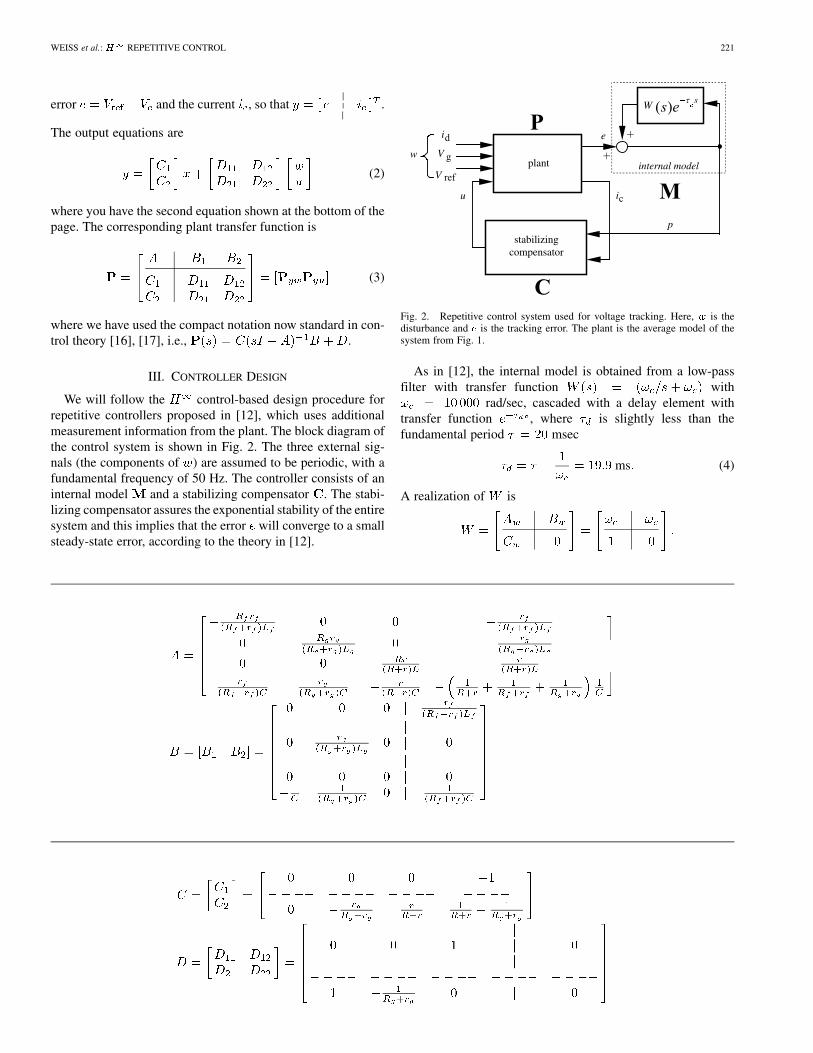
We will follow the control-based design procedure forrepetitive controllers proposed in [12], which uses additionalmeasurement information from the plant. The block diagram ofthe control system is shown in Fig. 2. The three external sig-nals (the components of ) are assumed to be periodic, with afundamental frequency of 50 Hz. The controller consists of aninternal model and a stabilizing compensator . The stabi-lizing compensator assures the exponential stability of the entiresystem and this implies that the error will converge to a smallsteady-state error, according to the theory in [12].

plant

stabilizingcompensator

internal model

p

i

e

w

i

V

W

V

u

Fig. 2. Repetitive control system used for voltage tracking. Here, w is thedisturbance and e is the tracking error. The plant is the average model of thesystem from Fig. 1.

As in [12], the internal model is obtained from a low-passfilter with transfer function with

rad/sec, cascaded with a delay element withtransfer function , where is slightly less than thefundamental period msec

ms (4)

A realization of is


After closing a positive unity feedback around this cascade con-nection, as shown in Fig. 2, we obtain the internal model

(5)

has an infinite sequence of pairs of conjugate poles of whichabout the first 30 are very close to the imaginary axis, aroundinteger multiples of , and the later ones arefurther to the left (see Appendix A for more details). The choiceof is based on a compromise: for too low, only a few polesof the internal model will be close to the imaginary axis, leadingto poor tracking and disturbance rejection at higher frequencies.For too high, the system is difficult to be stabilized (a stabi-lizing compensator may not exist, or it may need unreasonablyhigh bandwidth).

According to [12], the closed-loop system in Fig. 2 is ex-ponentially stable if the finite-dimensional closed-loop systemfrom Fig. 3 is stable and its transfer function from to , de-noted , satisfies . The intuitive explanation forthis is that in the control system of Fig. 2 a delay line is con-nected from the output to the input appearing in Fig. 3. Tomake this interconnected system stable, by the small gain the-orem, it is sufficient to make the gain from to less than 1 atall frequencies.

Thus, we have to design (the transfer function of the sta-bilizing compensator) such that the above two conditions aresatisfied. Moreover, we want to minimize , where

. Indeed, we know from([12] Section V) that a small value for will resultin a small steady-state error.

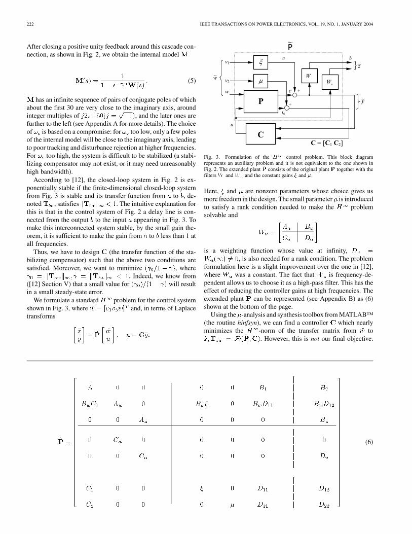
We formulate a standard problem for the control systemshown in Fig. 3, where and, in terms of Laplacetransforms

Fig. 3. Formulation of the H control problem. This block diagramrepresents an auxiliary problem and it is not equivalent to the one shown inFig. 2. The extended plant ~P consists of the original plant P together with thefilters W and W and the constant gains � and �.

Here, and are nonzero parameters whose choice gives usmore freedom in the design. The small parameter is introducedto satisfy a rank condition needed to make the problemsolvable and

is a weighting function whose value at infinity,, is also needed for a rank condition. The problem

formulation here is a slight improvement over the one in [12],where was a constant. The fact that is frequency-de-pendent allows us to choose it as a high-pass filter. This has theeffect of reducing the controller gains at high frequencies. Theextended plant can be represented (see Appendix B) as (6)shown at the bottom of the page.

Using the -analysis and synthesis toolbox from MATLAB™(the routine hinfsyn), we can find a controller which nearlyminimizes the -norm of the transfer matrix from to

. However, this is not our final objective.

(6)


We denote the central sub-optimal controller for a given-norm of by

(note that its feedthrough matrix is equal to 0). After some ma-nipulations (see Appendices C and D), we obtain the realiza-tions of and , respectively, as (7) and (8), shown at thebottom of the page. It is worth noting that (6)–(8) are valid forthe general case, regardless of the dimension of the measure-ment vector, which here is the scalar , and for any and .

Using the parameters shown in Table I, a nearly optimal con-troller, for which the Bode plots are shown in Fig. 4, was ob-tained for

(the latter two were determined via an extensive search to mini-mize while keeping ). The Bode plots showthat this controller is not realistic, because it has a very largebandwidth. Normally, the high-frequency poles can be reducedusing various controller/model reduction techniques, which is atopic of wide interest. Here, we use a different approach fromthat used in [18], [8], [9] to decrease the controller bandwidth:we do not minimize the -norm of but find a sub-optimal controller such that (which islarger than the minimal value 17.37). Such a controller (ob-tained using the hinfsyn routine in MATLAB is (9), shown atthe bottom of the page. It is easy to check that issatisfied for this . The pole with the highest frequency cre-ates a peak of the controller Bode plots at

rad/sec, as can be seen in Fig. 5. This is well belowhalf of the switching frequency rad/s,which is the same as the sampling frequency of the processorused to implement the controller. We used this as the stabi-lizing compensator in Fig. 2, for the simulations presented inthe next section. We have also done simulations with the dis-cretized controller (at the sampling frequency indicated above)and the results were very close to those for the continuous-timecontroller.

40

20

0

20

40

Mag

nitu

de (

dB)

100

102

104

106

108

1010

1012

90

45

0

45

90

Pha

se (

deg)

Bode plots of C1

Frequency (rad/sec)

40

20

0

20

40

Mag

nitu

de (

dB)

100

102

104

106

108

1010

1012

90

45

0

45

90

Pha

se (

deg)

Bode plots of C2

Frequency (rad/sec)

(a)

(b)

Fig. 4. Bode plots of a nearly optimal controller C for the H problemcorresponding to Fig. 3. Note that it has a very large bandwidth, which is notrealistic, given the switching frequency of 10 kHz. (a): Bode plots oc C . (b)Bode plots oc C .

(7)

(8)

(9)


12010080604020

02040

Mag

nitu

de (

dB)

100

102

104

106

108

1010

1012

135

90

45

0

45

90

Pha

se (

deg)

Bode plots of C1

Frequency (rad/sec)

(a)

12010080604020

02040

Mag

nitu

de (

dB)

100

102

104

106

108

1010

1012

135

90

45

0

45

90

Pha

se (

deg)

Bode plots of C2

Frequency (rad/sec)

(b)

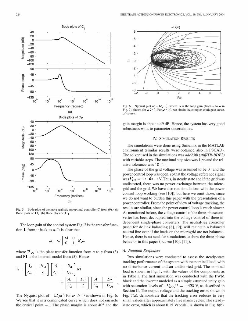
Fig. 5. Bode plots of the more realistic suboptimal controllerC from (9). (a):Bode plots oc C , (b) Bode plots oc C .

The loop gain of the control system Fig. 2 is the transfer func-tion from back to . It is clear that

where is the plant transfer function from to from (3)and is the internal model from (5). Hence

The Nyquist plot of for is shown in Fig. 6.We see that it is a complicated curve which does not encirclethe critical point . The phase margin is about 40 and the

2 1 0 1 2 3 4 5 6

0

2

4

6

8

Re

Im

L(jω)

2

4

6

8

Fig. 6. Nyquist plot of �L(j!), where L is the loop gain (from u to u inFig. 2), shown for ! � 0. For ! � 0, we obtain the complex conjugate curve,of course.

gain margin is about 4.49 dB. Hence, the system has very goodrobustness w.r.t. to parameter uncertainties.

IV. SIMULATION RESULTS

The simulations were done using Simulink in the MATLABenvironment (similar results were obtained also in PSCAD).The solver used in the simulations was ode23tb (stiff/TR-BDF2)with variable steps. The maximal step size was 1 s and the rel-ative tolerance was .

The phase of the grid voltage was assumed to be 0 and thepower control loop was open, so that the voltage reference signalwas V. Thus, in steady state and if the grid wasundistorted, there was no power exchange between the micro-grid and the grid. We have also run simulations with the powercontrol loop working (see [10]), but here we omit those, sincewe do not want to burden this paper with the presentation of apower controller. From the point of view of voltage tracking, theresults are similar, since the power control loop is much slower.As mentioned before, the voltage control of the three-phase con-verter has been decoupled into the voltage control of three in-dependent single-phase converters. The neutral-leg controller(used for dc link balancing [8], [9]) will maintain a balancedneutral line even if the loads on the microgrid are not balanced.Hence, there is no need for simulations to show the three-phasebehavior in this paper (but see [10], [11]).

A. Nominal Responses

Two simulations were conducted to assess the steady-statetracking performance of the system with the nominal load, withno disturbance current and an undistorted grid. The nominalload is shown in Fig. 1, with the values of the components asin Table I. The first simulation was conducted with the PWMblock and the inverter modeled as a simple saturated unity gainwith saturation levels of V, as described inSection II. The output voltage and the tracking error, shown inFig. 7(a), demonstrate that the tracking error reduces to verysmall values after approximately five mains cycles. The steady-state error, which is about 0.15 V(peak), is shown in Fig. 8(b).


0 0.05 0.1 0.15 0. 2400

300

200

100

0

100

200

300

400

Time (sec)

Vol

tage

(v)

V c e

0 0.05 0.1 0.15 0. 2400

300

200

100

0

100

200

300

400

Time (sec)

Vol

tage

(v)

V c e

0.36 0.37 0.38 0.39 0. 410

8

6

4

2

0

2

4

6

8

10

Time (sec)

Err

or (

v)

(a) (b)

(c)

Fig. 7. Output voltage V and the tracking error e, without a current disturbance (i = 0) and with the nominal load. (a) With the PWM block and the invertermodeled as a simple saturation. (b) With a detailed (not average) model of the PWM block and the inverter (f = 10 kHz). (c) The steady-state tracking errorsimulated with a detailed model of the PWM block and the inverter. The white line shows the steady-state tracking error simulated with the PWM block and theinverter modeled as a unity gain with saturation, i.e., without switching noise.

The second simulation used a detailed inverter model includinga PWM block, switching at 10 kHz. The response is shown inFig. 7(b). The results are similar but there is switching noisepresent that increases the steady-state tracking error which nowhas ripples of approximately 7 V(peak), as shown in Fig. 7(c).The controller is unable to suppress the switching noise, becauseit can only update the input to the pulse-width modulator onceper carrier cycle. The THD of the output voltage isaround 1.37%, almost all due to the switching noise, as Fig. 7(c)shows.

We mention that the curves in Fig. 7(a) and (b) do not showthe actual start-up process of an inverter with the nominal load,because the power controller is not present to ensure that thepower changes smoothly from zero to the desired value. Thesecurves only show the behavior of the voltage controller.

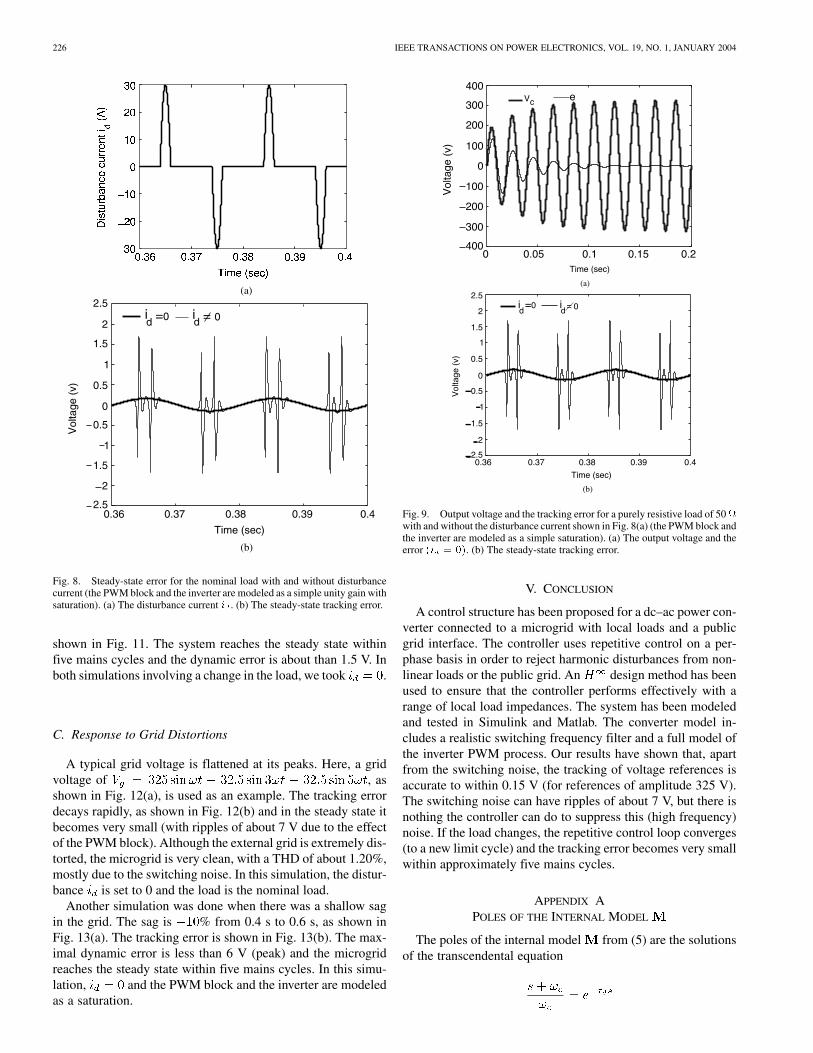
Fig. 8(b) shows the results of subjecting the plant to a dis-turbance current shown in Fig. 8(a), which has the typicalshape of the distortion caused by a capacitive rectifier. The peaksof are about half the nominal load current. As can be seen,the system has a good capability to reject such a disturbance.Indeed, the output current of the converter has a THD of16.38%, but the THD of the microgrid voltage is only 0.16%.

If we use a detailed model of the PWM block and the inverter,then the THD of increases slightly to 16.45%, while the THDof the microgrid voltage becomes 1.39%.

B. Response to Load Changes

Simulations were done when the load is a pure resistor of50 , which absorbs about 10% of the load power used in theprevious subsection. The PWM block and the inverter were stillmodeled as a saturation. The output voltage is shown in Fig. 9(a)and the tracking errors, with and without the disturbance cur-rent shown in Fig. 8(a), are shown in Fig. 9(b). No performancedegradation can be observed from these figures (with respect tothe nominal load).

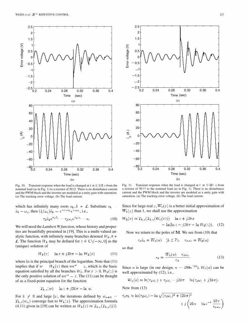
A more involved simulation explored the transient responseswhen the load is changed from the nominal load to a pure re-sistor of 50 . The tracking error and the current are shownin Fig. 10. The load is changed at s (when the loadcurrent is close to 0 so that the resulting spikes are small). Thesystem reaches the steady state within fpur mains cycles andthe dynamic error is less than 1.5 V. The response of the reverseprocess (changing the load from 50 to the nominal load) is


0.36 0.37 0.38 0.39 0.42.5

2

1.5

1

0.5

0

0.5

1

1.5

2id =0 = 0i

d

Vol

tage

(v)

Time (sec)

2.5(a)

(b)

Fig. 8. Steady-state error for the nominal load with and without disturbancecurrent (the PWM block and the inverter are modeled as a simple unity gain withsaturation). (a) The disturbance current i . (b) The steady-state tracking error.

shown in Fig. 11. The system reaches the steady state withinfive mains cycles and the dynamic error is about than 1.5 V. Inboth simulations involving a change in the load, we took .

C. Response to Grid Distortions

A typical grid voltage is flattened at its peaks. Here, a gridvoltage of , asshown in Fig. 12(a), is used as an example. The tracking errordecays rapidly, as shown in Fig. 12(b) and in the steady state itbecomes very small (with ripples of about 7 V due to the effectof the PWM block). Although the external grid is extremely dis-torted, the microgrid is very clean, with a THD of about 1.20%,mostly due to the switching noise. In this simulation, the distur-bance is set to 0 and the load is the nominal load.

Another simulation was done when there was a shallow sagin the grid. The sag is % from 0.4 s to 0.6 s, as shown inFig. 13(a). The tracking error is shown in Fig. 13(b). The max-imal dynamic error is less than 6 V (peak) and the microgridreaches the steady state within five mains cycles. In this simu-lation, and the PWM block and the inverter are modeledas a saturation.

Fig. 9. Output voltage and the tracking error for a purely resistive load of 50with and without the disturbance current shown in Fig. 8(a) (the PWM block andthe inverter are modeled as a simple saturation). (a) The output voltage and theerror (i = 0). (b) The steady-state tracking error.

V. CONCLUSION

A control structure has been proposed for a dc–ac power con-verter connected to a microgrid with local loads and a publicgrid interface. The controller uses repetitive control on a per-phase basis in order to reject harmonic disturbances from non-linear loads or the public grid. An design method has beenused to ensure that the controller performs effectively with arange of local load impedances. The system has been modeledand tested in Simulink and Matlab. The converter model in-cludes a realistic switching frequency filter and a full model ofthe inverter PWM process. Our results have shown that, apartfrom the switching noise, the tracking of voltage references isaccurate to within 0.15 V (for references of amplitude 325 V).The switching noise can have ripples of about 7 V, but there isnothing the controller can do to suppress this (high frequency)noise. If the load changes, the repetitive control loop converges(to a new limit cycle) and the tracking error becomes very smallwithin approximately five mains cycles.

APPENDIX APOLES OF THE INTERNAL MODEL

The poles of the internal model from (5) are the solutionsof the transcendental equation


0.2 0.24 0.28 0.32 0.36 0.4

1

0

0.5

1

1.5

2

2.5

Time (sec)

Err

or v

olta

ge (

V)

0.5

1.5

2.5

2

0.2 0.24 0.28 0.32 0.36 0.4 80

60

40

20

0

20

40

60

80

Time (sec)

i c (A

)

(a)

(b)

Fig. 10. Transient response when the load is changed at t = 0:301 s from thenominal load (as in Fig. 1) to a resistor of 50 . There is no disturbance currentand the PWM block and the inverter are modeled as a unity gain with saturation.(a) The tracking error voltage. (b) The load current.

which has infinitely many roots . Substitute, then i.e.,

(10)

We will need the Lambert W function, whose history and proper-ties are beautifully presented in [19]. This is a multi-valued an-alytic function, with infinitely many branches denoted

. The function may be defined for as the(unique) solution of

(11)

where is the principal branch of the logarithm. Note that (11)implies that if then , which is the basicequation satisfied by all the branches . For isthe only positive solution of . The (11) can be thoughtof as a fixed-point equation for the function

For and large , the iterations defined byconverge fast to . The approximation formula

(4.11) given in [19] can be written as .

0.2 0.24 0.28 0.32 0.36 0.4 2.5

2

1.5

1

0.5

0

0.5

1

1.5

2

2.5

Time (sec)

Err

or v

olta

ge (

V)

0.2 0.24 0.28 0.32 0.36 0.4 80

60

40

20

0

20

40

60

80

Time (sec)

i c (A

)

(a)

(b)

Fig. 11. Transient response when the load is changed at t = 0:301 s froma resistor of 50 to the nominal load (as in Fig. 1). There is no disturbancecurrent and the PWM block and the inverter are modeled as a unity gain withsaturation. (a) The tracking error voltage. (b) The load current.

Since for large real is a better initial approximation ofthan 1, we shall use the approximation

(12)

Now we return to the poles of . We see from (10) that

so that

(13)

Since is large (in our design, ), can bewell approximated by (12), i.e.,

Now from (13)


0.36 0.37 0.38 0.39 0.4400

300

200

100

0

100

200

300

400

Vol

tage

(V

) micro-grid

(external) grid

Time (sec)

0 0.1 0.2 0.3 0.4200

150

100

50

0

50

100

150

200

Time (sec)

Vol

tage

(V

)

(a)

(b)Fig. 12. Effect of a distorted public grid: the grid voltages and the trackingerror. In this simulation, we have used a detailed model of the PWM blockand the inverter. The switching noise is visible in the plot of the error. (a) Thesteady-state grid voltages. (b) The transient tracking error.

so that

(14)

(15)

The last approximation holds because ifthen we may approximate by the identity function. Theseapproximated poles and the true poles are shown in Fig. 14for , and we have checked that the approximation isvery good even for . Ideally, we would like to have

. At least, we want this to be approximately truefor small . In order to make , according to(15), we need to satisfy . Solving thisequation, we obtain

(16)

The solution with a minus sign is not reasonable, since it wouldlead to and then many of the approximations usedearlier would break down. The reasonable solution correspondsto the plus sign in (16) and then a good approximation of ,when is large, is

as in (4). This coincides with the recommendation in ([12], Sec-tion II). However, when is not so large, should be chosenaccording to (16) with the plus sign.

APPENDIX BREALIZATION OF

Here we derive (6), the realization of the extended plant. Wehave from Fig. 3

If we combine the above equations, then we obtain (6).

APPENDIX CREALIZATION OF

Here we derive (7). Assume in Fig. 3 and ,then , where satisfies

Substitute into (1), then

and from (2)


Fig. 13. Effect of a shallow sag of �10% in the grid voltage from t = 0:4 s to t = 0:6 s. (a) The (external) grid voltage. (b) The microgrid voltage. (c) Thetransient tracking error.

Furthermore

Hence, the transfer matrix from to is the first equation at thebottom of the page.

APPENDIX DREALIZATION OF

Here we derive (8). Assume in Fig. 3 and , then

and , where

so that . Hence, the transfer matrixfrom to is the second equation at the bottom of the page.


18 16 14 12 10 8 6 4 2 01

0.8

0.6

0.4

0.2

0

0.2

0.4

0.6

0.8

1x 10

4

Re

Im

true poles

approximated poles * o

Fig. 14. Poles s of the internal model M for jkj � 31. Note that thehorizontal scale is much smaller than the vertical scale, so that these polesare actually almost on the imaginary axis. Here, the approximation formulae(14)–(15) were used.

ACKNOWLEDGMENT

The authors wish to thank the Editors and the Reviewers fortheir careful work and helpful advice on this paper.

REFERENCES

[1] N. Jenkins, R. Allan, P. Crossley, D. Kirschen, and G. Strbac, EmbeddedGeneration, ser. IEE Power and Energy Series: IEE Books, 2000.

[2] Z. Chen and E. Spooner, “Grid power quality with variable speed windturbines,” IEEE Trans. Energy Conv., vol. 16, pp. 148–154, June 2001.

[3] M. Etezadi-Amoli and K. Choma, “Electrical performance characteris-tics of a new microturbine generator,” in Proc. IEEE Power Eng. Soc.Winter Meeting, vol. 2, 2001, pp. 736–740.

[4] J. Enslin, M. Wolf, D. Snyman, and W. Swiegers, “Integrated photo-voltaic maximum power point tracking converter,” IEEE Trans. Ind.Electron., vol. 44, pp. 769–773, Dec. 1997.

[5] R. Lasseter, “MicroGrids,” Proc. IEEE Power Eng. Soc. Winter Meeting,vol. 1, pp. 305–308, 2002.

[6] G. Venkataramanan and M. Illindala, “Microgrids and sensitive loads,”Proc. IEEE Power Eng. Soc. Winter Meeting, vol. 1, pp. 315–322, 2002.

[7] T. Green and M. Prodanovic, “Control of inverter-based microgrids,”Electric Power Syst. Res., Special Issue Distributed Generation, 2003.

[8] Q.-C. Zhong, T. Green, J. Liang, and G. Weiss, “H control of theneutral leg for three-phase four-wire dc–ac converters,” in Proc. 28thAnnu. Conf. IEEE Ind. Electron. Soc. (IECON’02), Seville, Spain, Nov.2002.

[9] Q.-C. Zhong and G. Weiss, “H control of the neutral leg for three-phase four-wire dc-ac converters,” IEEE Trans. Ind. Electron., submittedfor publication.

[10] J. Liang, T. Green, G. Weiss, and Q.-C. Zhong, “Decoupling controlof the active and reactive power for a grid-connected three-phase dc-acinverter,” in Proc. Eur. Contr. Conf., Cambridge, MA, U.K., Sept. 2003.

[11] , “Evaluation of repetitive control for power quality improvementof distributed generation,” in Proc. 33rd IEEE Annu. Power Electron.Spec. Conf., vol. 4, Queensland, Autralia, June 2002, pp. 1803–1808.

[12] G. Weiss and M. Hafele, “Repetitive control of MIMO systems usingH design,” Automatica, vol. 35, no. 7, pp. 1185–1199, 1999.

[13] Y. Yamamoto, “Learning control and related problems in infinite-di-mensional systems,” in Essays on Control: Perspectives in the Theoryand Its Applications, H. Trentelman and J. Willems, Eds. Boston, MA:Birkhäuser, 1993, pp. 191–222.

[14] K. Zhou, D. Wang, and K.-S. Low, “Periodic errors elimination in CVCFPWM dc/ac converter systems: Repetitive control approach,” Proc. Inst.Elect. Eng., vol. 147, no. 6, pp. 694–700, 2000.

[15] K. Zhou and D. Wang, “Digital repetitive learning controller for three-phase CVCF PWM inverter,” IEEE Trans. Ind. Electron., vol. 48, pp.820–830, Aug. 2001.

[16] K. Zhou and J. Doyle, Essentials of Robust Control. Upper SaddleRiver, N.J.: Prentice-Hall, 1998.

[17] M. Green and D. Limebeer, Linear Robust Control. Englewood Cliffs,NJ: Prentice-Hall, 1995.

[18] R. Naim, G. Weiss, and S. Ben-Yaakov, “H control applied to boostpower converters,” IEEE Trans. Power Electron., vol. 12, pp. 677–683,July 1997.

[19] R. Corless, G. Gonnet, D. Hare, D. Jeffrey, and D. Knuth, “On the Lam-bert W function,” Adv. Computat. Math, vol. 5, pp. 329–359, 1996.

George Weiss received the Control Engineer degree from the Polytechnic In-stitute of Bucharest, Romania, in 1981 and the Ph.D. degree in applied mathe-matics from the Weizmann Institute, Rehovot, Israel, in 1989.

He has been with Brown University, Providence, RI, the Virginia PolytechnicInstitute and State University, Blacksburg, the Weizmann Institute, Ben-GurionUniversity, Beer Sheva, Israel, the University of Exeter, U.K., and is currentlywith Imperial College London, U.K. His research interests are distributed pa-rameter systems, operator semigroups, power electronics, repetitive control, andperiodic (in particular, sampled-data) linear systems.

Qing-Chang Zhong was born in 1970 in Sichuan,China. He received the M.S. degree in electrical en-gineering from Hunan University, China, in 1997 andthe Ph.D. degree in control theory and engineeringfrom Shanghai Jiao Tong University, China, in 1999.

He started working in the area of control engi-neering in 1990 after graduating from the XiangtanInstitute of Mechanical and Electrical Technology(now renamed as Hunan Institute of Engineering).He held a postdoctoral position at Technion-IsraelInstitute of Technology, Israel, from 2000 to 2001.

He is currently a Research Associate at the Department of Electrical andElectronic Engineering, Imperial College London, U.K. His current researchfocuses on H-infinity control of time-delay systems, control in power elec-tronics, process control, control in communication networks, and control usingdelay elements such as input shaping technique and repetitive control.

Tim C. Green (M’89–SM’02) received the B.Sc.(with first class honors) degree from ImperialCollege, London, U.K., in 1986 and the Ph.D. degreefrom Heriot-Watt University, Edinburgh, U.K., in1990, both in electrical engineering.

He was a Lecturer at Heriot Watt University, U.K.,until 1994 and is now a Reader at Imperial CollegeLondon and member of the Control and Power Re-search Group. His research interest is in using powerelectronics and control to enhance power quality andpower delivery. This covers FACTS, active power fil-

ters, distributed generation and un-interruptible supplies.Dr. Green is a Chartered Engineer in the U.K. and a member of the IEE.

Jun Liang (M’02) received the B.S. degree in elec-trical engineering from Huazhong University of Sci-ence and Technology, China, in 1992 and the M.S.and Ph.D. degrees in electrical engineering from theElectric Power Research Institute (EPRI), China, in1995 and 1998, respectively.

He was with EPRI, from 1998 to 2001 as a SeniorEngineer, and is currently a Research Associate in theDepartment of Electrical and Electronic Engineering,Imperial College London. His research interests arepower electronics, power system control, renewable

power generation, and distributed generation.

h repetitive control of dc-ac converters in microgrids - spiral

Documents