national bank of poland working paper no. 124
TRANSCRIPT

On the empirical importance of periodicity in the volatility of financial time series
Warsaw 2012
Błażej Mazur�, Mateusz Pipień
NATIONAL BANK OF POLANDWORKING PAPER
No. 124

Design:
Oliwka s.c.
Layout and pr�int:
NBP Pr�intshop
Published by:
National Bank of Poland Education and Publishing Depar�tment 00-919 War�szawa, 11/21 Świętokr�zyska Str�eet phone: +48 22 653 23 35, fax +48 22 653 13 21
© Copyr�ight by the National Bank of Poland, 2012
ISSN 2084–624X
http://www.nbp.pl
Błażej Mazur� – Economic Institute, National Bank of Poland and Depar�tment of Econometr�ics and Oper�ations Resear�ch, Cr�acow Univer�sity of EconomicsMateusz Pipień – Economic Institute, National Bank of Poland and Depar�tment of Econometr�ics and Oper�ations Resear�ch, Cr�acow Univer�sity of Economics
Contents
1 Introduction 3
2 A simple nonstationary process obtained from the GARCH(1,1)
model 5
3 A model for periodic volatility 9
4 Basic model framework and posterior inference 12
5 Empirical analysis 15
6 Conclusion 19
1

WORKING PAPER No. 124 1
Contents
Contents
1 Introduction 3
2 A simple nonstationary process obtained from the GARCH(1,1)
model 5
3 A model for periodic volatility 9
4 Basic model framework and posterior inference 12
5 Empirical analysis 15
6 Conclusion 19
1

Abstr�act
N a t i o n a l B a n k o f P o l a n d2
Abstract
We discuss the empirical importance of long term cyclical effects in the
volatility of financial returns. Following C̆iz̆ek and Spokoiny (2009), Amado and
Teräsvirta (2012) and others, we consider a general conditionally heteroscedastic
process with stationarity property distorted by a deterministic function that
governs the possible variability in time of unconditional variance. The function
proposed in this paper can be interpreted as a finite Fourier approximation of an
Almost Periodic (AP) function as defined by Corduneanu (1989). The resulting
model has a particular form of a GARCH process with time varying parameters,
intensively discussed in the recent literature.
In the empirical analyses we apply a generalisation of the Bayesian AR(1)-t-
GARCH(1,1) model for daily returns of S&P500, covering the period of sixty
years of US postwar economy, including the recently observed global financial
crisis. The results of a formal Bayesian model comparison clearly indicate the
existence of significant long term cyclical patterns in volatility with a strongly
supported periodic component corresponding to a 14 year cycle. This may be
interpreted as empirical evidence in favour of a linkage between the business cycle
in the US economy and long term changes in the volatility of the basic stock
market index.
Keywords: Periodically correlated stochastic processes, GARCH models, Bayesian
inference, volatility, unconditional variance
JEL classification: C58, C11, G10
2
1 Introduction
Starting from seminal works by Clark (1973), Engle (1982) and Bollerslev (1986)
stochastic processes used to describe observed properties of the volatility of financial
time series have been tailored to identify short term features. In particular, the
resurgence of stochastic volatility (SV) models in the 90’s relied on the assumption
that there exists a stochastic factor independent of the past of the process, which
influences volatility in the short term. The resulting literature concerning GARCH
and SV models, its properties and practical importance is enormous, however empirical
analyses of the dynamic behaviour of the volatility in the long term has not been fully
explored so far.
Recently, some attempts to model long term features of volatility have been made.
Since empirical analyses of long time series of financial returns clearly indicated that
parameters of volatility models may vary over time, it is obvious that models applied so
far may not capture properties of volatility which are important in the long term. At the
beginning of the 90’s the GARCH-type models became a very popular tool of volatility
modelling. But parallelly some problems were identified with their applications to
long time series of financial returns. For example, Lamoreux and Lastrapes (1990)
and Engle and Mustafa (1992) suggested that parameters of GARCH-type processes
are very strongly identified , because while in econometric applications their estimates
are statistically highly significant, they are not stable over time. Consequently, the
constancy of parameters initially imposed in GARCH-type processes was subject to
criticism that prompted new studies concerning generalisations. In particular Mikosh
and Stărică (2004) indicate that the IGARCH effect is often spuriously supported
by data, because in the case of long time series variability of parameters is natural.
Hence the regular GARCH(1,1) structure is unable to capture nonlinearity and
possible complex stochastic properties of the observed process. Teräsvirta (2009)
points out a more formal motivation in favour of time variability of parameters in a
parametric GARCH scheme, suggesting that constancy of parameters can be a testable
restriction and if it is rejected, the model should be generalised. Several approaches
3

Intr�oduction
WORKING PAPER No. 124 3
1
Abstract
We discuss the empirical importance of long term cyclical effects in the
volatility of financial returns. Following C̆iz̆ek and Spokoiny (2009), Amado and
Teräsvirta (2012) and others, we consider a general conditionally heteroscedastic
process with stationarity property distorted by a deterministic function that
governs the possible variability in time of unconditional variance. The function
proposed in this paper can be interpreted as a finite Fourier approximation of an
Almost Periodic (AP) function as defined by Corduneanu (1989). The resulting
model has a particular form of a GARCH process with time varying parameters,
intensively discussed in the recent literature.
In the empirical analyses we apply a generalisation of the Bayesian AR(1)-t-
GARCH(1,1) model for daily returns of S&P500, covering the period of sixty
years of US postwar economy, including the recently observed global financial
crisis. The results of a formal Bayesian model comparison clearly indicate the
existence of significant long term cyclical patterns in volatility with a strongly
supported periodic component corresponding to a 14 year cycle. This may be
interpreted as empirical evidence in favour of a linkage between the business cycle
in the US economy and long term changes in the volatility of the basic stock
market index.
Keywords: Periodically correlated stochastic processes, GARCH models, Bayesian
inference, volatility, unconditional variance
JEL classification: C58, C11, G10
2
1 Introduction
Starting from seminal works by Clark (1973), Engle (1982) and Bollerslev (1986)
stochastic processes used to describe observed properties of the volatility of financial
time series have been tailored to identify short term features. In particular, the
resurgence of stochastic volatility (SV) models in the 90’s relied on the assumption
that there exists a stochastic factor independent of the past of the process, which
influences volatility in the short term. The resulting literature concerning GARCH
and SV models, its properties and practical importance is enormous, however empirical
analyses of the dynamic behaviour of the volatility in the long term has not been fully
explored so far.
Recently, some attempts to model long term features of volatility have been made.
Since empirical analyses of long time series of financial returns clearly indicated that
parameters of volatility models may vary over time, it is obvious that models applied so
far may not capture properties of volatility which are important in the long term. At the
beginning of the 90’s the GARCH-type models became a very popular tool of volatility
modelling. But parallelly some problems were identified with their applications to
long time series of financial returns. For example, Lamoreux and Lastrapes (1990)
and Engle and Mustafa (1992) suggested that parameters of GARCH-type processes
are very strongly identified , because while in econometric applications their estimates
are statistically highly significant, they are not stable over time. Consequently, the
constancy of parameters initially imposed in GARCH-type processes was subject to
criticism that prompted new studies concerning generalisations. In particular Mikosh
and Stărică (2004) indicate that the IGARCH effect is often spuriously supported
by data, because in the case of long time series variability of parameters is natural.
Hence the regular GARCH(1,1) structure is unable to capture nonlinearity and
possible complex stochastic properties of the observed process. Teräsvirta (2009)
points out a more formal motivation in favour of time variability of parameters in a
parametric GARCH scheme, suggesting that constancy of parameters can be a testable
restriction and if it is rejected, the model should be generalised. Several approaches
3
Intr�oduction
N a t i o n a l B a n k o f P o l a n d4
1
have been proposed imposing time variability of parameters in volatility models. We
see two basic fundamental approaches applied in this respect, the first one relates
to variability governed by a random process, and the second relies on deterministic
framework. Within the confines of the first approach, Hamilton and Susmel (1994)
conducted research on the empirical importance of the assumption that stock returns
are characterised by different ARCH processes at different points in time, with the shifts
between processes mediated by a Markov chain. This straightforward approach opened
new topics in financial econometrics based on the application of Markov switching
mechanisms in volatility modelling. A possible variability of parameters described
by a deterministic function was also subject to analysis. Teräsvirta (2009) modified
the smooth transition GARCH model by imposing a transition function of the form
that guarantees variability of parameters for a process observed in finite time interval.
The transition function depends on the length of the observed time series. C̆iz̆ek
and Spokoiny (2009) present a review of literature concluding that relaxing time
homogeneity of the process is a promising approach but causes serious problems with
proper estimation methods. For instance, when some or all model parameters will vary
over time, a more subtle treatment of testing structural breaks in financial returns
may be obtained; see Fan and Zhang (1999), Cai et al. (2000), Fan et al. (2003). An
approach to the specification of time varying GARCH models was developed in the field
of nonparametric statistics. Under very general conditions concerning the regularity
of parameters treated as functions of time, nonparametric methods of estimation were
proposed; see Härdle et al. (2003), Mercurio and Spokoiny (2004), Spokoiny and Chen
(2007) and C̆iz̆ek and Spokoiny (2009).
The main purpose of this paper is to propose a simple generalisation of the GARCH
model which would enable to model long term features of volatility. Our construct is
strictly related to the literature studying the properties of GARCH processes with time
varying parameters and is based on parametric approach; see Teräsvirta (2009), Amado
and Teräsvirta (2012). The variability of unconditional moments is governed by a class
of Almost Periodic (AP) functions, proposed by Corduneanu (1989) as a generalisation
of the class of periodic functions. Since in our approach the unconditional second
4
moment exhibits almost periodic variability, the process can be also interpreted as a
second order Almost Periodically Correlated (APC) stochastic process, discussed from
the theoretical point of view by Hurd and Miamee (2007). During the last five decades
the APC class of processes was broadly applied in telecommunication (Gardner (1986),
Napolitano and Spooner (2001)), climatology (Bloomfield et al. (1994)) and many other
fields. For an exhaustive review of possible applications see Gardner et al. (2006).
We make a formal statistical inference, from the Bayesian viewpoint, about the
cyclicality of volatility changes and present evidence in favour of the empirical
importance of such an effect. On the basis of very intuitive explanation of almost
periodicity, we provide an economic interpretation of time variability of unconditional
moments supported by data. The illustration is conducted on the basis of daily returns
of the S&P500 index covering the period from 18 January 1950 till 7 February 2012.
2 A simple nonstationary process obtained from the
GARCH(1,1) model
We start from a general definition of a conditionally heteroscedastic model which nests
many GARCH-type volatility models developed during more than the last four decades
in the field of financial econometrics.
Definition 1. Discrete, real valued, stochastic process {ξt, t ∈ Z} is called
conditionally heteroscedastic if:
ξt =√
ht(ω, Ψt−1)zt, zt ∼ iid,
where ht(ω, Ψt−1) constitutes volatility equation, defined as a parametric function of
the information set Ψt−1 = (. . . , ξt−2, ξt−1), i.e. the history of the process {ξt, t ∈ Z},
and parameters ω. Random variables zt are identically and independently distributed.
Any conditionally heteroskedastic GARCH-type model, defined in the literature,
starting from the ARCH(p) model proposed by Engle (1982) and the GARCH(p,q),
proposed by Bollerslev (1986), can be obtained by imposing some particular functional
5

A simple nonstationar�y pr�ocess obtained fr�om the GARCH(1,1) model
WORKING PAPER No. 124 5
2
have been proposed imposing time variability of parameters in volatility models. We
see two basic fundamental approaches applied in this respect, the first one relates
to variability governed by a random process, and the second relies on deterministic
framework. Within the confines of the first approach, Hamilton and Susmel (1994)
conducted research on the empirical importance of the assumption that stock returns
are characterised by different ARCH processes at different points in time, with the shifts
between processes mediated by a Markov chain. This straightforward approach opened
new topics in financial econometrics based on the application of Markov switching
mechanisms in volatility modelling. A possible variability of parameters described
by a deterministic function was also subject to analysis. Teräsvirta (2009) modified
the smooth transition GARCH model by imposing a transition function of the form
that guarantees variability of parameters for a process observed in finite time interval.
The transition function depends on the length of the observed time series. C̆iz̆ek
and Spokoiny (2009) present a review of literature concluding that relaxing time
homogeneity of the process is a promising approach but causes serious problems with
proper estimation methods. For instance, when some or all model parameters will vary
over time, a more subtle treatment of testing structural breaks in financial returns
may be obtained; see Fan and Zhang (1999), Cai et al. (2000), Fan et al. (2003). An
approach to the specification of time varying GARCH models was developed in the field
of nonparametric statistics. Under very general conditions concerning the regularity
of parameters treated as functions of time, nonparametric methods of estimation were
proposed; see Härdle et al. (2003), Mercurio and Spokoiny (2004), Spokoiny and Chen
(2007) and C̆iz̆ek and Spokoiny (2009).
The main purpose of this paper is to propose a simple generalisation of the GARCH
model which would enable to model long term features of volatility. Our construct is
strictly related to the literature studying the properties of GARCH processes with time
varying parameters and is based on parametric approach; see Teräsvirta (2009), Amado
and Teräsvirta (2012). The variability of unconditional moments is governed by a class
of Almost Periodic (AP) functions, proposed by Corduneanu (1989) as a generalisation
of the class of periodic functions. Since in our approach the unconditional second
4
moment exhibits almost periodic variability, the process can be also interpreted as a
second order Almost Periodically Correlated (APC) stochastic process, discussed from
the theoretical point of view by Hurd and Miamee (2007). During the last five decades
the APC class of processes was broadly applied in telecommunication (Gardner (1986),
Napolitano and Spooner (2001)), climatology (Bloomfield et al. (1994)) and many other
fields. For an exhaustive review of possible applications see Gardner et al. (2006).
We make a formal statistical inference, from the Bayesian viewpoint, about the
cyclicality of volatility changes and present evidence in favour of the empirical
importance of such an effect. On the basis of very intuitive explanation of almost
periodicity, we provide an economic interpretation of time variability of unconditional
moments supported by data. The illustration is conducted on the basis of daily returns
of the S&P500 index covering the period from 18 January 1950 till 7 February 2012.
2 A simple nonstationary process obtained from the
GARCH(1,1) model
We start from a general definition of a conditionally heteroscedastic model which nests
many GARCH-type volatility models developed during more than the last four decades
in the field of financial econometrics.
Definition 1. Discrete, real valued, stochastic process {ξt, t ∈ Z} is called
conditionally heteroscedastic if:
ξt =√
ht(ω, Ψt−1)zt, zt ∼ iid,
where ht(ω, Ψt−1) constitutes volatility equation, defined as a parametric function of
the information set Ψt−1 = (. . . , ξt−2, ξt−1), i.e. the history of the process {ξt, t ∈ Z},
and parameters ω. Random variables zt are identically and independently distributed.
Any conditionally heteroskedastic GARCH-type model, defined in the literature,
starting from the ARCH(p) model proposed by Engle (1982) and the GARCH(p,q),
proposed by Bollerslev (1986), can be obtained by imposing some particular functional
5

A simple nonstationar�y pr�ocess obtained fr�om the GARCH(1,1) model
N a t i o n a l B a n k o f P o l a n d6
2
form of ht(ω, Ψt−1).
For further analysis let us consider the discrete and real valued stochastic process
{εt, t ∈ Z} defined as follows:
εt =√
g(t, γ)ξt, (1)
where {ξt, t ∈ Z} is defined by Definition 1, and g(., γ) is a positive real valued
function of time domain Z, parameterised by γ. The following theorem presents obvious
necessary and sufficient conditions of moment existence for the process {εt, t ∈ Z}.
The form of the process {εt, t ∈ Z} is related to the general specification considered
by Amado and Teräsvirta (2012). The aim of our study is a proper specification of
function g, so that it has an economic interpretation and is empirically important.
Theorem 1. For a process {εt, t ∈ Z} in (1), where {ξt, t ∈ Z} is given by Definition
1 we have the following equivalences:
1. For each n ∈ N , E(εnt ) exists and E(εn
t ) = g(t, γ)n2 E(ξn
t ) if and only if E(ξnt )
exists
2. For each n ∈ N , E(εnt |Ψt−1) exists and E(εn
t |Ψt−1) = g(t, γ)n2 ht(θ, Ψt−1)
n2 E(zn
t )
if and only if E(znt ) exists.
As an example of the process in Definition 1 let us consider the seminal Generalised
Autoregressive Conditional Heteroskedastic (GARCH) process, initially defined by
Bollerslev (1986). Formally Bollerslev (1986) defined GARCH(p,q) process for any
natural p and q by defining lag of squared residuals and conditional variance applied in
the volatility equation. According to Engle (1985) who stated that the GARCH(1,1)
is the leading generic model for almost all asset classes of returns [...] it is quite robust
and does most of the work in almost all cases, we focus our attention on the case with
p = 1 and q = 1. In the definition of GARCH(1,1) process we follow Bauwens, Lubrano
and Richard (1999) setting.
Definition 2. A discrete, real valued, stochastic process {ξt, t ∈ Z} is called
GARCH(1,1) if:
ξt =√
htzt,
6
where
ht = α0 + α1ξ2t−1 + β1ht−1,
for α0 ≥ 0, α1 > 0, β1 > 0. Random variables zt are identically and independently
distributed in such a way, that:
1. E(zt) = 0
2. E(z2t ) = 1
3. E(z3t ) = 0
4. E(z4t ) = λ > 0.
When analysing stochastic properties of the process in Definition 2, it is crucial to
pay attention on the restriction α1 + β1 < 1. It ensures moment existence up to the
second order and its stability over time and, consequently, covariance stationarity of the
process. The GARCH(1,1) process with α1 + β1 = 1 is called IGARCH. This case still
represents the process stationary in the strict sense, but covariance stationarity is no
longer fulfilled. Bauwens, Lubrano and Richard (1999) listed the following properties
of the GARCH(1,1) process:
Theorem 2. If the process {ξt, t ∈ Z} follows Definition 2, then:
1. E(ξt|Ψt−1) = 0
2. V (ξt) = E(ξ2t |Ψt−1) = ht
3. E(ξ3t |Ψt−1) = 0
4. E(ξ4t |Ψt−1) = λh2
t
5. K(ξ4t |Ψt−1) = λ
6. E(ξt) = 0
7. E(ξ2t ) =
α0
1 − α1 − β1if additionally α1 + β1 < 1
8. E(ξ3t ) = 0
7

A simple nonstationar�y pr�ocess obtained fr�om the GARCH(1,1) model
WORKING PAPER No. 124 7
2
form of ht(ω, Ψt−1).
For further analysis let us consider the discrete and real valued stochastic process
{εt, t ∈ Z} defined as follows:
εt =√
g(t, γ)ξt, (1)
where {ξt, t ∈ Z} is defined by Definition 1, and g(., γ) is a positive real valued
function of time domain Z, parameterised by γ. The following theorem presents obvious
necessary and sufficient conditions of moment existence for the process {εt, t ∈ Z}.
The form of the process {εt, t ∈ Z} is related to the general specification considered
by Amado and Teräsvirta (2012). The aim of our study is a proper specification of
function g, so that it has an economic interpretation and is empirically important.
Theorem 1. For a process {εt, t ∈ Z} in (1), where {ξt, t ∈ Z} is given by Definition
1 we have the following equivalences:
1. For each n ∈ N , E(εnt ) exists and E(εn
t ) = g(t, γ)n2 E(ξn
t ) if and only if E(ξnt )
exists
2. For each n ∈ N , E(εnt |Ψt−1) exists and E(εn
t |Ψt−1) = g(t, γ)n2 ht(θ, Ψt−1)
n2 E(zn
t )
if and only if E(znt ) exists.
As an example of the process in Definition 1 let us consider the seminal Generalised
Autoregressive Conditional Heteroskedastic (GARCH) process, initially defined by
Bollerslev (1986). Formally Bollerslev (1986) defined GARCH(p,q) process for any
natural p and q by defining lag of squared residuals and conditional variance applied in
the volatility equation. According to Engle (1985) who stated that the GARCH(1,1)
is the leading generic model for almost all asset classes of returns [...] it is quite robust
and does most of the work in almost all cases, we focus our attention on the case with
p = 1 and q = 1. In the definition of GARCH(1,1) process we follow Bauwens, Lubrano
and Richard (1999) setting.
Definition 2. A discrete, real valued, stochastic process {ξt, t ∈ Z} is called
GARCH(1,1) if:
ξt =√
htzt,
6
where
ht = α0 + α1ξ2t−1 + β1ht−1,
for α0 ≥ 0, α1 > 0, β1 > 0. Random variables zt are identically and independently
distributed in such a way, that:
1. E(zt) = 0
2. E(z2t ) = 1
3. E(z3t ) = 0
4. E(z4t ) = λ > 0.
When analysing stochastic properties of the process in Definition 2, it is crucial to
pay attention on the restriction α1 + β1 < 1. It ensures moment existence up to the
second order and its stability over time and, consequently, covariance stationarity of the
process. The GARCH(1,1) process with α1 + β1 = 1 is called IGARCH. This case still
represents the process stationary in the strict sense, but covariance stationarity is no
longer fulfilled. Bauwens, Lubrano and Richard (1999) listed the following properties
of the GARCH(1,1) process:
Theorem 2. If the process {ξt, t ∈ Z} follows Definition 2, then:
1. E(ξt|Ψt−1) = 0
2. V (ξt) = E(ξ2t |Ψt−1) = ht
3. E(ξ3t |Ψt−1) = 0
4. E(ξ4t |Ψt−1) = λh2
t
5. K(ξ4t |Ψt−1) = λ
6. E(ξt) = 0
7. E(ξ2t ) =
α0
1 − α1 − β1if additionally α1 + β1 < 1
8. E(ξ3t ) = 0
7

A simple nonstationar�y pr�ocess obtained fr�om the GARCH(1,1) model
N a t i o n a l B a n k o f P o l a n d8
2
9. E(ξ4t ) = λα2
0
1 + α1 + β1
(1 − λα21 − β2
1 − 2α1β1)(1 − α1 − β1)if additionally α1+β1 < 1 and
λα21 + β2
1 + 2α1λ < 1
10. K(ξt) = λ(1 − α1 − β1)(1 + α1 + β1)
1 − λα21 − β2
1 − 2α1β1
11. Corr(ξ2t , ξ2
t−1) =α1(1 − β2
1 − α1β1)1 − β2
1 − 2α1β1if additionally α1 + β1 < 1
12. Corr(ξ2t , ξ2
t−k) = (α1 + β1)Corr(ξ2t , ξ2
t−k−1) = (α1 + β1)k−1 α1(1 − β21 − α1β1)
1 − β21 − 2α1β1
if
additionally α1 + β1 < 1,
where K(ξ) denotes kurtosis for a random variable ξ and Corr(ξ1, ξ2) denotes
correlation between ξ1 and ξ2.
According to Theorem 2, given restriction α1 +β1 < 1, process {ξt, t ∈ Z} is covariance
stationary with unconditional zero mean and finite unconditional variance V (ξt) =
E(ξ2t ) =
α0
1 − α1 − β1. Also, autocovariance function for any nonzero lag is equal to
zero. However for squares of the process, again if α1 +β1 < 1, autocorrelation function
is not constant and decays at exponential rate as a function of lag. Now let consider the
process {εt, t ∈ Z} defined by (1), generated by the GARCH(1,1) process {ξt, t ∈ Z}.
Automatically from Theorem 1 we obtain the following properties:
Theorem 3. If the process {εt, t ∈ Z} is defined by equation (1) and {ξt, t ∈ Z} in
(1) follows Definition 2, then:
E(εt|Ψt−1) = 0
E(ε2t |Ψt−1) = g(t, γ)ht
E(ε3t |Ψt−1) = 0
E(ε4t |Ψt−1) = λg(t, γ)2h2
t
K(ε4t |Ψt−1) = λ
E(εt) = 0
V (εt) = E(ε2t ) = g(t, γ)
α0
1 − α1 − β1, if additionally α1 + β1 < 1
E(ε3t ) = 0
8
E(ε4t ) = g(t, γ)2λα2
0
1 + α1 + β1
(1 − λα21 − β2
1 − 2α1λ)(1 − α1 − β1)if additionally α1 + β1 < 1
and λα21 + β2
1 + 2α1λ < 1
K(εt) = λ(1 − α1 − β1)(1 + α1 + β1)
1 − λα21 − β2
1 − 2α1β1= K(ξt)
Corr(ε2t , ε
2t−1) = Corr(ξ2
t , ξ2t−1) if additionally α1 + β1 < 1
Corr(ε2t , ε
2t−k) = Corr(ξ2
t , ξ2t−k) if additionally α1 + β1 < 1.
It is clear from Theorem 3, that process {εt, t ∈ Z} is nonstationary in the strict
sense and also covariance nonstationary. Function g(f(., γ) assures variability of
unconditional moments, especially the unconditional variance given by formula 7 in
Theorem 3. Also variability over time of conditional variance of yt is decomposed
into GARCH(1,1) effect and deterministic component, that changes dispersion of the
conditional distribution according to the form of function g. From the definition of
process {zt, t ∈ Z} we keep the first and the third moment, and also kurtosis of
εt, unchanged. Consequently our construct generates a nonstationary process with
time-varying unconditional second order moments and with an additional source of
variability of the conditional variance.
Another interesting feature of {εt, t ∈ Z} can be observed if we rewrite the equation
for conditional variance in GARCH-type form. If the process {εt, t ∈ Z} is defined by
equation (1) and {ξt, t ∈ Z} in (1) follows Definition 2, we have:
E(ε2t |Ψt−1) = g(t, γ)ht = α0,t + α1,tξ
2t−1 + β1,tht−1, (2)
where α0,t = g(t, γ)α0, α1,t = g(t, γ)α1 and β1,t = g(t, γ)β1. Hence, the process {εt, t ∈
Z} can be also interpreted as a GARCH(1,1) model with time varying parameters.
3 A model for periodic volatility
The main purpose of the paper is a proper definition of function g in (1), that would
enable the testing the variability of parameters in (2) but also provide an economic
interpretation of such an effect.The vast literature concerning time-varying GARCH
models does not seem to explore this aspect in detail, focusing only on the statistical
9

A model for� per�iodic volatility
WORKING PAPER No. 124 9
3
9. E(ξ4t ) = λα2
0
1 + α1 + β1
(1 − λα21 − β2
1 − 2α1β1)(1 − α1 − β1)if additionally α1+β1 < 1 and
λα21 + β2
1 + 2α1λ < 1
10. K(ξt) = λ(1 − α1 − β1)(1 + α1 + β1)
1 − λα21 − β2
1 − 2α1β1
11. Corr(ξ2t , ξ2
t−1) =α1(1 − β2
1 − α1β1)1 − β2
1 − 2α1β1if additionally α1 + β1 < 1
12. Corr(ξ2t , ξ2
t−k) = (α1 + β1)Corr(ξ2t , ξ2
t−k−1) = (α1 + β1)k−1 α1(1 − β21 − α1β1)
1 − β21 − 2α1β1
if
additionally α1 + β1 < 1,
where K(ξ) denotes kurtosis for a random variable ξ and Corr(ξ1, ξ2) denotes
correlation between ξ1 and ξ2.
According to Theorem 2, given restriction α1 +β1 < 1, process {ξt, t ∈ Z} is covariance
stationary with unconditional zero mean and finite unconditional variance V (ξt) =
E(ξ2t ) =
α0
1 − α1 − β1. Also, autocovariance function for any nonzero lag is equal to
zero. However for squares of the process, again if α1 +β1 < 1, autocorrelation function
is not constant and decays at exponential rate as a function of lag. Now let consider the
process {εt, t ∈ Z} defined by (1), generated by the GARCH(1,1) process {ξt, t ∈ Z}.
Automatically from Theorem 1 we obtain the following properties:
Theorem 3. If the process {εt, t ∈ Z} is defined by equation (1) and {ξt, t ∈ Z} in
(1) follows Definition 2, then:
E(εt|Ψt−1) = 0
E(ε2t |Ψt−1) = g(t, γ)ht
E(ε3t |Ψt−1) = 0
E(ε4t |Ψt−1) = λg(t, γ)2h2
t
K(ε4t |Ψt−1) = λ
E(εt) = 0
V (εt) = E(ε2t ) = g(t, γ)
α0
1 − α1 − β1, if additionally α1 + β1 < 1
E(ε3t ) = 0
8
E(ε4t ) = g(t, γ)2λα2
0
1 + α1 + β1
(1 − λα21 − β2
1 − 2α1λ)(1 − α1 − β1)if additionally α1 + β1 < 1
and λα21 + β2
1 + 2α1λ < 1
K(εt) = λ(1 − α1 − β1)(1 + α1 + β1)
1 − λα21 − β2
1 − 2α1β1= K(ξt)
Corr(ε2t , ε
2t−1) = Corr(ξ2
t , ξ2t−1) if additionally α1 + β1 < 1
Corr(ε2t , ε
2t−k) = Corr(ξ2
t , ξ2t−k) if additionally α1 + β1 < 1.
It is clear from Theorem 3, that process {εt, t ∈ Z} is nonstationary in the strict
sense and also covariance nonstationary. Function g(f(., γ) assures variability of
unconditional moments, especially the unconditional variance given by formula 7 in
Theorem 3. Also variability over time of conditional variance of yt is decomposed
into GARCH(1,1) effect and deterministic component, that changes dispersion of the
conditional distribution according to the form of function g. From the definition of
process {zt, t ∈ Z} we keep the first and the third moment, and also kurtosis of
εt, unchanged. Consequently our construct generates a nonstationary process with
time-varying unconditional second order moments and with an additional source of
variability of the conditional variance.
Another interesting feature of {εt, t ∈ Z} can be observed if we rewrite the equation
for conditional variance in GARCH-type form. If the process {εt, t ∈ Z} is defined by
equation (1) and {ξt, t ∈ Z} in (1) follows Definition 2, we have:
E(ε2t |Ψt−1) = g(t, γ)ht = α0,t + α1,tξ
2t−1 + β1,tht−1, (2)
where α0,t = g(t, γ)α0, α1,t = g(t, γ)α1 and β1,t = g(t, γ)β1. Hence, the process {εt, t ∈
Z} can be also interpreted as a GARCH(1,1) model with time varying parameters.
3 A model for periodic volatility
The main purpose of the paper is a proper definition of function g in (1), that would
enable the testing the variability of parameters in (2) but also provide an economic
interpretation of such an effect.The vast literature concerning time-varying GARCH
models does not seem to explore this aspect in detail, focusing only on the statistical
9

A model for� per�iodic volatility
N a t i o n a l B a n k o f P o l a n d10
3
properties of estimation methods, given very general assumptions about the variability
of parameters.
Some attempts to interpret time heterogeneity of processes describing volatility have
been made. One of them was adopted by Hamilton (1989). In this seminal paper formal
statistical representation of the old idea that expansion and contraction constitute two
distinct economic phases was considered. Hamilton proposed to model real output
growth by two autoregressions, depending on whether the economy is expanding or
contracting. Possible changes between those autoregressions were governed by a Markov
chain. The main contribution of Hamilton (1989) was a very intuitive economic
interpretation of a purely random construct as a factor governing changes between
states of different intensity of economic activity. This idea was easily instilled in
modelling financial time series, where Markov switching ARCH and GARCH models
were specifically developed for volatility modelling; see Hamilton and Susmel (1994),
Susmel (2000), Haas et al. (2004), Li and Lin (2004) and many others. Just like in the
case of the business cycle, Markov switching volatility models are able to distinguish
phases of low and high volatility, or - in the case of many regimes - many different
levels of risk intensity. However, as concluded by Langa and Rahbek (2009), in spite of
the fact that Markov switching volatility models have recently received much interest
in applications, a sufficiently complete theory for these models is still missing. Some
theoretical aspects concerning properties of forecasts were presented; see for example
Amendola and Niglio (2004). Yet, in Markov switching conditionally heteroscedastic
models basic conditions that would guarantee stationarity are still unknown.
Another disadvantage of Hamilton’s approach is that different phases of intensity
of volatility change abruptly, according to a random process in time domain. The
resulting path of the volatility process has discontinuities at points where a change
of regime was observed. This leaves the application of the whole Hamilton’s idea in
volatility modelling with doubts. Analogously to modelling economic activity of the
real sector, the volatility of financial time series also seems to have phases of expansion
and contraction in the long term. An analysis of financial returns in the span of
decades shows that changes between states are much closer to continuous rather than
10
discrete. Since those phases alternate in cases of boom and bust on the market, on a
large scale volatility should also exhibit cyclical behaviour. In order to test for such an
effect, a stochastic process with an approximately periodic structure of unconditional
moments should be considered. For a process {εt, t ∈ Z} defined by equation (1),
where {ξt, t ∈ Z} in (1) follows Definition 2, it can easily be done on the basis of
an appropriately defined function g(., γ), which describes the variability of moments.
In general, we follow the idea of generalisation of periodicity of real valued functions
proposed by Corduneanu (1989).
Definition 3. A real-valued function f : Z −→ R of an integer variable is called almost
periodic (AP in short), if for any ε > 0 there exists an integer Lε > 0, such that among
any Lε consecutive integers, there is an integer pε with the property
supt∈Z
|f(t + pε) − f(t)| < ε.
Any periodic function is also almost periodic. Conditions from Definition 3 constitute
a class of almost periodically correlated (APC) stochastic processes as a generalisation
of periodically correlated (PC) stochastic processes. In the case of APC processes,
an almost periodic function, and in the case of PC processes, a periodic function,
determines the cyclical variability of conditional and unconditional moments. Therefore
PC stochastic processes are also called cyclostationary. During the last five decades
the APC class was broadly applied in telecommunication (Gardner (1986)), Napolitano
and Spooner (2001)), climatology (Bloomfield et al. (1994)) and many other fields. For
exhaustive review of possible applications see Gardner et al. (2006).
The main properties of the APC class was presented by Corduneanu (1989). In
particular, any almost periodic function from Definition 3 has its unique Fourier
expansion of the form:
f(t) =∞∑i=1
(gsi sin(hit) + gci cos(hit)) , (3)
with the series of coefficients (gsi)∞i=1, (gci)∞i=1 and (hi)∞i=1 that express amplitude and
11

A model for� per�iodic volatility
WORKING PAPER No. 124 11
3
properties of estimation methods, given very general assumptions about the variability
of parameters.
Some attempts to interpret time heterogeneity of processes describing volatility have
been made. One of them was adopted by Hamilton (1989). In this seminal paper formal
statistical representation of the old idea that expansion and contraction constitute two
distinct economic phases was considered. Hamilton proposed to model real output
growth by two autoregressions, depending on whether the economy is expanding or
contracting. Possible changes between those autoregressions were governed by a Markov
chain. The main contribution of Hamilton (1989) was a very intuitive economic
interpretation of a purely random construct as a factor governing changes between
states of different intensity of economic activity. This idea was easily instilled in
modelling financial time series, where Markov switching ARCH and GARCH models
were specifically developed for volatility modelling; see Hamilton and Susmel (1994),
Susmel (2000), Haas et al. (2004), Li and Lin (2004) and many others. Just like in the
case of the business cycle, Markov switching volatility models are able to distinguish
phases of low and high volatility, or - in the case of many regimes - many different
levels of risk intensity. However, as concluded by Langa and Rahbek (2009), in spite of
the fact that Markov switching volatility models have recently received much interest
in applications, a sufficiently complete theory for these models is still missing. Some
theoretical aspects concerning properties of forecasts were presented; see for example
Amendola and Niglio (2004). Yet, in Markov switching conditionally heteroscedastic
models basic conditions that would guarantee stationarity are still unknown.
Another disadvantage of Hamilton’s approach is that different phases of intensity
of volatility change abruptly, according to a random process in time domain. The
resulting path of the volatility process has discontinuities at points where a change
of regime was observed. This leaves the application of the whole Hamilton’s idea in
volatility modelling with doubts. Analogously to modelling economic activity of the
real sector, the volatility of financial time series also seems to have phases of expansion
and contraction in the long term. An analysis of financial returns in the span of
decades shows that changes between states are much closer to continuous rather than
10
discrete. Since those phases alternate in cases of boom and bust on the market, on a
large scale volatility should also exhibit cyclical behaviour. In order to test for such an
effect, a stochastic process with an approximately periodic structure of unconditional
moments should be considered. For a process {εt, t ∈ Z} defined by equation (1),
where {ξt, t ∈ Z} in (1) follows Definition 2, it can easily be done on the basis of
an appropriately defined function g(., γ), which describes the variability of moments.
In general, we follow the idea of generalisation of periodicity of real valued functions
proposed by Corduneanu (1989).
Definition 3. A real-valued function f : Z −→ R of an integer variable is called almost
periodic (AP in short), if for any ε > 0 there exists an integer Lε > 0, such that among
any Lε consecutive integers, there is an integer pε with the property
supt∈Z
|f(t + pε) − f(t)| < ε.
Any periodic function is also almost periodic. Conditions from Definition 3 constitute
a class of almost periodically correlated (APC) stochastic processes as a generalisation
of periodically correlated (PC) stochastic processes. In the case of APC processes,
an almost periodic function, and in the case of PC processes, a periodic function,
determines the cyclical variability of conditional and unconditional moments. Therefore
PC stochastic processes are also called cyclostationary. During the last five decades
the APC class was broadly applied in telecommunication (Gardner (1986)), Napolitano
and Spooner (2001)), climatology (Bloomfield et al. (1994)) and many other fields. For
exhaustive review of possible applications see Gardner et al. (2006).
The main properties of the APC class was presented by Corduneanu (1989). In
particular, any almost periodic function from Definition 3 has its unique Fourier
expansion of the form:
f(t) =∞∑i=1
(gsi sin(hit) + gci cos(hit)) , (3)
with the series of coefficients (gsi)∞i=1, (gci)∞i=1 and (hi)∞i=1 that express amplitude and
11

Basic model framework and posterior inference
N a t i o n a l B a n k o f P o l a n d12
4
frequency of individual cyclical component in (3).
For further research concerning cyclical behavior of volatility, we consider the following
function g(., γ) in (1):
g(t, γ) = ef(t,γ), (4)
where
f(t, γ) =F∑
i=1
(γsi sin(φit) + γci cos(φit)) , (5)
with γ = (γs1, ..., γsF , γc1, ..., γcF , φ1, ..., φF ). Function f(., γ) is defined as a sum of
periodic functions, with parameters φi determining frequencies, while γsi and γci control
amplitudes. Since we limit the infinite series to its finite substitute, formula (5) yields
finite approximation of order F of the almost periodic function, that governs moment
variability of the process.
The case γsi = 0 and γci = 0 for all i = 1, ..., F , in (5), determines constant function
g(., γ) ≡ 1. According to Hurd and Miamee (2007), the process {εt, t ∈ Z} defined by
equation (1), where {ξt, t ∈ Z} in (1) follows Definition 2 is also Almost Periodically
Correlated. According to the properties shown in the previous section, the function
g(., γ) in (5) enables to model the existence of cyclicality in the conditional and
unconditional variance of the process. This property will be subject to formal statistical
inference in the empirical part of the paper.
4 Basic model framework and posterior inference
We model logarithmic returns on the financial instrument with price xt at time t.
Suppose, we observe time series of logarithmic returns given by the form:
yt = 100 lnxt
xt−1, t = −1, 0, 1, . . . , T.
Denote by y = (y1, . . . , yT ) the vector of modelled observations. Daily returns y−1 and
y0 are used as initial values.
Just like many authors, in order to model the dynamics of financial returns we assume
an AR(1) process with nonstationary disturbances of the following form; see for example
12
Bauwens, Lubrano and Richard (1999) for univariate case or Osiewalski and Pipień
(2004) for multivariate setting:
yt = µt + εt, t = 1, . . . , T, (6)
where µt = δ + ρ(yt−1 − δ) and εt is a process defined by (3), i.e.:
εt =√
f(t, γ)ξt, t = 1, . . . , T,
with the GARCH(1,1) process ξt from Definition 2:
ξt =√
htzt, ht = α0 + α1ξ2t−1 + β1ht−1 t = 1, . . . , T,
and function f given by (3). We assume, that random variables zt in Definition 2 are
independent and follow Student-t distribution with zero mean, unit variance and ν > 4
degrees of freedom. In the literature, conditional Student-t distribution is applied in
GARCH models, with standard restriction ν > 2 imposed, that assures existence of
conditional variance. However, in order to keep all conditions in definition 2 fulfilled,
we have to assume, that ν > 4. Given this stronger restriction E(z4t ) = λ = 3
ν − 2ν − 4
.
The density of zt is given by the formula:
fs(zt|0, 1, ν) =Γ(ν+1
2 )
Γ(ν2 )
√π(ν − 2)
[1 +
z2t
ν − 2
]− ν+12
,
where fs(zt|m, s2, ν) denotes the density of the Student-t distribution with mean m,
variance s2 and ν > 4 degrees o freedom.
The conditional distributions of ξt and εt are Student-t distributions with zero mean,
ν > 4 degrees o freedom and variances ht and g(t, γ)ht respectively:
p(ξt|Ψt−1) = fs(ξt|0, ht, ν) =Γ(ν+1
2 )
Γ(ν2 )
√π(ν − 2)ht
[1 +
ξ2t
(ν − 2)ht
]− ν+12
,
p(εt|Ψt−1) = fs(εt|0, g(t, γ)ht, ν) =Γ(ν+1
2 )
Γ(ν2 )
√π(ν − 2)g(t, γ)ht
[1 +
ε2t
(ν − 2)g(t, γ)ht
]− ν+12
,
13

Basic model framework and posterior inference
WORKING PAPER No. 124 13
4
frequency of individual cyclical component in (3).
For further research concerning cyclical behavior of volatility, we consider the following
function g(., γ) in (1):
g(t, γ) = ef(t,γ), (4)
where
f(t, γ) =F∑
i=1
(γsi sin(φit) + γci cos(φit)) , (5)
with γ = (γs1, ..., γsF , γc1, ..., γcF , φ1, ..., φF ). Function f(., γ) is defined as a sum of
periodic functions, with parameters φi determining frequencies, while γsi and γci control
amplitudes. Since we limit the infinite series to its finite substitute, formula (5) yields
finite approximation of order F of the almost periodic function, that governs moment
variability of the process.
The case γsi = 0 and γci = 0 for all i = 1, ..., F , in (5), determines constant function
g(., γ) ≡ 1. According to Hurd and Miamee (2007), the process {εt, t ∈ Z} defined by
equation (1), where {ξt, t ∈ Z} in (1) follows Definition 2 is also Almost Periodically
Correlated. According to the properties shown in the previous section, the function
g(., γ) in (5) enables to model the existence of cyclicality in the conditional and
unconditional variance of the process. This property will be subject to formal statistical
inference in the empirical part of the paper.
4 Basic model framework and posterior inference
We model logarithmic returns on the financial instrument with price xt at time t.
Suppose, we observe time series of logarithmic returns given by the form:
yt = 100 lnxt
xt−1, t = −1, 0, 1, . . . , T.
Denote by y = (y1, . . . , yT ) the vector of modelled observations. Daily returns y−1 and
y0 are used as initial values.
Just like many authors, in order to model the dynamics of financial returns we assume
an AR(1) process with nonstationary disturbances of the following form; see for example
12
Bauwens, Lubrano and Richard (1999) for univariate case or Osiewalski and Pipień
(2004) for multivariate setting:
yt = µt + εt, t = 1, . . . , T, (6)
where µt = δ + ρ(yt−1 − δ) and εt is a process defined by (3), i.e.:
εt =√
f(t, γ)ξt, t = 1, . . . , T,
with the GARCH(1,1) process ξt from Definition 2:
ξt =√
htzt, ht = α0 + α1ξ2t−1 + β1ht−1 t = 1, . . . , T,
and function f given by (3). We assume, that random variables zt in Definition 2 are
independent and follow Student-t distribution with zero mean, unit variance and ν > 4
degrees of freedom. In the literature, conditional Student-t distribution is applied in
GARCH models, with standard restriction ν > 2 imposed, that assures existence of
conditional variance. However, in order to keep all conditions in definition 2 fulfilled,
we have to assume, that ν > 4. Given this stronger restriction E(z4t ) = λ = 3
ν − 2ν − 4
.
The density of zt is given by the formula:
fs(zt|0, 1, ν) =Γ(ν+1
2 )
Γ(ν2 )
√π(ν − 2)
[1 +
z2t
ν − 2
]− ν+12
,
where fs(zt|m, s2, ν) denotes the density of the Student-t distribution with mean m,
variance s2 and ν > 4 degrees o freedom.
The conditional distributions of ξt and εt are Student-t distributions with zero mean,
ν > 4 degrees o freedom and variances ht and g(t, γ)ht respectively:
p(ξt|Ψt−1) = fs(ξt|0, ht, ν) =Γ(ν+1
2 )
Γ(ν2 )
√π(ν − 2)ht
[1 +
ξ2t
(ν − 2)ht
]− ν+12
,
p(εt|Ψt−1) = fs(εt|0, g(t, γ)ht, ν) =Γ(ν+1
2 )
Γ(ν2 )
√π(ν − 2)g(t, γ)ht
[1 +
ε2t
(ν − 2)g(t, γ)ht
]− ν+12
,
13

Basic model framework and posterior inference
N a t i o n a l B a n k o f P o l a n d14
4
where Ψ0 = (h0, y−1, y0), and Ψt−1 = (Ψ0, y1, . . . , tt−1) = (Ψ0, y(t−1)). Consequently,
the conditional distribution of daily return in (6) is Student-t distribution with mean
µt = δ + ρ(yt−1 − δ), variance g(t, γ)ht and ν > 4 degrees of freedom:
p(yt|Ψt−1) = fs(yt|µt, g(t, γ)ht, ν) =Γ(ν+1
2 )
Γ(ν2 )
√π(ν − 2)g(t, γ)ht
[1 +
(yt − µt)2
(ν − 2)g(t, γ)ht
]− ν+12
.
(7)
Let θ denote the vector, that contains all model parameters. We assume, that
θ = (µ‘, σ2‘, ν, γ‘)‘ where vectors µ = (δ, ρ)‘, σ2 = (α0, α1, β1)‘ and γ =
(γs1, ..., γsF , γc1, ..., γcF , φ1, ..., φF ) collect parameters of the conditional mean of yt,
the conditional variance of ε and function g respectively. According to (7), we define
the sampling model for a vector y as follows:
p(y|θ) =T∏
t=1
p(yt|Ψt−1) =T∏
t=1
fs(yt|µt, g(t, γ)ht, ν).
The Bayesian model, i.e. the joint distribution of observables and parameters, requires
specification of the prior distribution p(θ). We assume the following prior independence:
p(y, θ) = p(y|θ)p(θ) = p(y|θ)p(δ)p(ρ)p(α0)p(α1, β1)p(ν)p(γ),
where p(δ) is normal distribution, p(ρ) is uniform over (-1,1), p(α0) is exponential
distribution with unit mean, p(α1, β1) is bivariate uniform distribution on the unit
square [0, 1]2, p(ν) is exponential distribution with mean 10 truncated at ν > 4,
p(γ) is multivariate normal, p(φ) is multivariate uniform over the set generated by
identification restrictions that eliminates label-switching effect in (5). We assume,
that L < φ1 < . . . < φF < U , for appropriately chosen L and U , which eliminates
frequencies of length shorter than a quarter and longer than the time interval covering
the observed time series.
14
5 Empirical analysis
In this section we present the empirical analysis and make formal Bayesian inference
about the empirical importance of the cyclical component in the volatility of daily
returns of one of the most important US Stock Market indices. Our dataset consists
of T = 15615 observations of daily logarithmic returns of the S&P500 index, covering
the period starting from the postwar era of the US economy till the beginning of 2012.
The time series starts on 18 January 1950 and ends on 7 February 2012.
In Table 1 we present results of Bayesian model comparison, conducted for four
competing specifications. Initially we consider conditionally a Student-t AR(1)-
GARCH(1,1) process (denoted by M0). We also add APC(F)-GARCH(1,1) models
(denoted by MF ) for F=1,2 and 3 frequencies describing the variability of unconditional
moments according to (5). In Table 1 we show decimal logarithms of marginal data
densities, approximated by the Newton and Raftery (1994) estimator and decimal
logarithms of the Bayes factor in favour of the best model. The dataset strongly
supports time variability of parameters in GARCH(1,1) specification and consequently
nonstationarity in the strict sense. The original GARCH(1,1) model receives little data
support, as the marginal data density value is more than three orders of magnitude
lower than in the case of the worst APC model, i.e. in the case when unconditional
variance is described by a single cyclical component. The strongest data support goes
to APC(2)-GARCH(1,1) model, with the marginal data density value greater than in
the case of M0 by more than six orders of magnitude. Among competing specifications
with time-varying parameters the data substantially support the case where variability
of unconditional moments can be described by an Almost Periodic function of the form
(4) with different frequencies. The case with frequencies is also supported, however it
does not receive as great data support as the APC(2)-GARCH(1,1) case.
Table 2 presents results of Bayesian estimation of parameters in AR(1)-GARCH(1,1)
and APC(2)-GARCH(1,1) models (M0 and M2 respectively). We report the following
posterior summaries: the mean (E(.|y)), the modal value (Mod(.|y)) and the standard
deviation (D(.|y)) of the marginal distributions of parameters in both models. Posterior
15

Empirical analysis
WORKING PAPER No. 124 15
5
where Ψ0 = (h0, y−1, y0), and Ψt−1 = (Ψ0, y1, . . . , tt−1) = (Ψ0, y(t−1)). Consequently,
the conditional distribution of daily return in (6) is Student-t distribution with mean
µt = δ + ρ(yt−1 − δ), variance g(t, γ)ht and ν > 4 degrees of freedom:
p(yt|Ψt−1) = fs(yt|µt, g(t, γ)ht, ν) =Γ(ν+1
2 )
Γ(ν2 )
√π(ν − 2)g(t, γ)ht
[1 +
(yt − µt)2
(ν − 2)g(t, γ)ht
]− ν+12
.
(7)
Let θ denote the vector, that contains all model parameters. We assume, that
θ = (µ‘, σ2‘, ν, γ‘)‘ where vectors µ = (δ, ρ)‘, σ2 = (α0, α1, β1)‘ and γ =
(γs1, ..., γsF , γc1, ..., γcF , φ1, ..., φF ) collect parameters of the conditional mean of yt,
the conditional variance of ε and function g respectively. According to (7), we define
the sampling model for a vector y as follows:
p(y|θ) =T∏
t=1
p(yt|Ψt−1) =T∏
t=1
fs(yt|µt, g(t, γ)ht, ν).
The Bayesian model, i.e. the joint distribution of observables and parameters, requires
specification of the prior distribution p(θ). We assume the following prior independence:
p(y, θ) = p(y|θ)p(θ) = p(y|θ)p(δ)p(ρ)p(α0)p(α1, β1)p(ν)p(γ),
where p(δ) is normal distribution, p(ρ) is uniform over (-1,1), p(α0) is exponential
distribution with unit mean, p(α1, β1) is bivariate uniform distribution on the unit
square [0, 1]2, p(ν) is exponential distribution with mean 10 truncated at ν > 4,
p(γ) is multivariate normal, p(φ) is multivariate uniform over the set generated by
identification restrictions that eliminates label-switching effect in (5). We assume,
that L < φ1 < . . . < φF < U , for appropriately chosen L and U , which eliminates
frequencies of length shorter than a quarter and longer than the time interval covering
the observed time series.
14
5 Empirical analysis
In this section we present the empirical analysis and make formal Bayesian inference
about the empirical importance of the cyclical component in the volatility of daily
returns of one of the most important US Stock Market indices. Our dataset consists
of T = 15615 observations of daily logarithmic returns of the S&P500 index, covering
the period starting from the postwar era of the US economy till the beginning of 2012.
The time series starts on 18 January 1950 and ends on 7 February 2012.
In Table 1 we present results of Bayesian model comparison, conducted for four
competing specifications. Initially we consider conditionally a Student-t AR(1)-
GARCH(1,1) process (denoted by M0). We also add APC(F)-GARCH(1,1) models
(denoted by MF ) for F=1,2 and 3 frequencies describing the variability of unconditional
moments according to (5). In Table 1 we show decimal logarithms of marginal data
densities, approximated by the Newton and Raftery (1994) estimator and decimal
logarithms of the Bayes factor in favour of the best model. The dataset strongly
supports time variability of parameters in GARCH(1,1) specification and consequently
nonstationarity in the strict sense. The original GARCH(1,1) model receives little data
support, as the marginal data density value is more than three orders of magnitude
lower than in the case of the worst APC model, i.e. in the case when unconditional
variance is described by a single cyclical component. The strongest data support goes
to APC(2)-GARCH(1,1) model, with the marginal data density value greater than in
the case of M0 by more than six orders of magnitude. Among competing specifications
with time-varying parameters the data substantially support the case where variability
of unconditional moments can be described by an Almost Periodic function of the form
(4) with different frequencies. The case with frequencies is also supported, however it
does not receive as great data support as the APC(2)-GARCH(1,1) case.
Table 2 presents results of Bayesian estimation of parameters in AR(1)-GARCH(1,1)
and APC(2)-GARCH(1,1) models (M0 and M2 respectively). We report the following
posterior summaries: the mean (E(.|y)), the modal value (Mod(.|y)) and the standard
deviation (D(.|y)) of the marginal distributions of parameters in both models. Posterior
15

Empirical analysis
N a t i o n a l B a n k o f P o l a n d16
5
inference about common parameters (degrees of freedom ν and AR-GARCH parameters
i.e subvectors µ,σ2 in θ) remains almost the same in both models, as posterior
summaries change only slightly after incorporating a deterministic function f into the
volatility equation. The data support strong persistence of conditional variance, as
the sum α1 + β1 is located close to unity in case of model M0. The deterministic
component in the volatility equation of model M2 is empirically important, but it does
not change posterior location of α1 + β1 qualitatively. Also the posterior inference
about tails of the conditional distribution of returns is almost the same in both models,
leading to the conclusion that conditional normality is rejected even in the case of
nonstationarity of the error term. On the other hand, moment existence as imposed
according to Definition 2, is decisively supported, because posterior standard deviation
makes a less than 4 degrees of freedom parameter improbable in view of the data.
Generally, marginal posterior distributions of common parameters are very regular,
symmetric and qualitatively the same in the case of both models. In contrast, the
posterior distributions of model specific parameters in the APC(2)-GARCH(1,1) model
are irregular, as expectation and modal value in those cases may be located in different
areas of the parameter space. We see relative strong dispersion of parameters controlling
amplitudes in (5), namely γs1, γs2, γc1 and γc2. For frequency parameters φ1 and φ2 a
more regular posterior distribution was obtained.
Figure 1 presents results of posterior inference about the length of the period pi of
a single cyclical component in (3) induced by posterior distribution of the frequency
parameter φi. We show histograms of the length in years, according to the formula:
pi =2π
φi251,
assuming 251 trading days per year. We compare histograms between the best model
M2, where f is defined as a sum of two different cyclical components, and slightly worse
(but still enjoying strong data support) M1 model, with f defined by a single cyclical
component. In the case of the M2 model we see that one component, of approximately
14 years, is very precisely identified, as the majority of the probability mass of the
16
posterior distribution of p2 is located between the values of 13 and 15 years with the
mode and median equal approximately 14 years. However, the posterior inference
about the second cyclical component might be problematic due to a rather irregular
and dispersed posterior distribution. The posterior median for parameter p1 indicates
the existence of a much longer cycle, with the length greater than 30 years. However,
the probability mass of the posterior distribution is very dispersed, leaving considerably
greater uncertainty about the length of this longer cycle in unconditional variance.
In contrast to model M2, we obtain a very irregular posterior distribution of the length
of the cycle in model M1. According to the plot of the histogram of p1 we see how
problematic the inference about the possible cyclical behavior on unconditional variance
may be, given APC(1)-GARCH(1,1) specification. Since the marginal posterior
distribution of p1 is bimodal, any inference based on posterior summaries leads to
wrong conclusions. Posterior expectation is located in areas of domain completely
precluded in view of the data. We see, that the mass of posterior distribution is
located either around the value of p1 = 14 and in the regions, where p1 > 35. Formally
in model M1 the data support the length of the cycle equal approximately to 14 years,
as the posterior median is slightly greater than 14.17. But taking into account regions
identified by both local extremes we see that inference about the length of the cycle in
unconditional variance and the qualitative profile of the cyclical effect is rather similar
in both models M1 and M2. Since in model M1 there is only one cyclical component in
function f , the irregular shape of posterior distribution of p1 can be explained as clear
data support for two different frequencies in the equation for unconditional variance,
just like in model M2.
The effect of cyclicality in unconditional variance of the error term in (6) and its
empirical importance is depicted in Figure 2. We present the plot with absolute returns
and posterior means of unconditional variance calculated for each data point, with
bounds covering the range of two posterior standard deviations. We also plotted the
posterior mean of the unconditional variance in model M0, as a constant function
at E(V (εt)|y, M0) = 0.9889. Again, the data clearly support the variability of
unconditional variance. The constancy of parameters is precluded since the changes of
17

Empirical analysis
WORKING PAPER No. 124 17
5
inference about common parameters (degrees of freedom ν and AR-GARCH parameters
i.e subvectors µ,σ2 in θ) remains almost the same in both models, as posterior
summaries change only slightly after incorporating a deterministic function f into the
volatility equation. The data support strong persistence of conditional variance, as
the sum α1 + β1 is located close to unity in case of model M0. The deterministic
component in the volatility equation of model M2 is empirically important, but it does
not change posterior location of α1 + β1 qualitatively. Also the posterior inference
about tails of the conditional distribution of returns is almost the same in both models,
leading to the conclusion that conditional normality is rejected even in the case of
nonstationarity of the error term. On the other hand, moment existence as imposed
according to Definition 2, is decisively supported, because posterior standard deviation
makes a less than 4 degrees of freedom parameter improbable in view of the data.
Generally, marginal posterior distributions of common parameters are very regular,
symmetric and qualitatively the same in the case of both models. In contrast, the
posterior distributions of model specific parameters in the APC(2)-GARCH(1,1) model
are irregular, as expectation and modal value in those cases may be located in different
areas of the parameter space. We see relative strong dispersion of parameters controlling
amplitudes in (5), namely γs1, γs2, γc1 and γc2. For frequency parameters φ1 and φ2 a
more regular posterior distribution was obtained.
Figure 1 presents results of posterior inference about the length of the period pi of
a single cyclical component in (3) induced by posterior distribution of the frequency
parameter φi. We show histograms of the length in years, according to the formula:
pi =2π
φi251,
assuming 251 trading days per year. We compare histograms between the best model
M2, where f is defined as a sum of two different cyclical components, and slightly worse
(but still enjoying strong data support) M1 model, with f defined by a single cyclical
component. In the case of the M2 model we see that one component, of approximately
14 years, is very precisely identified, as the majority of the probability mass of the
16
posterior distribution of p2 is located between the values of 13 and 15 years with the
mode and median equal approximately 14 years. However, the posterior inference
about the second cyclical component might be problematic due to a rather irregular
and dispersed posterior distribution. The posterior median for parameter p1 indicates
the existence of a much longer cycle, with the length greater than 30 years. However,
the probability mass of the posterior distribution is very dispersed, leaving considerably
greater uncertainty about the length of this longer cycle in unconditional variance.
In contrast to model M2, we obtain a very irregular posterior distribution of the length
of the cycle in model M1. According to the plot of the histogram of p1 we see how
problematic the inference about the possible cyclical behavior on unconditional variance
may be, given APC(1)-GARCH(1,1) specification. Since the marginal posterior
distribution of p1 is bimodal, any inference based on posterior summaries leads to
wrong conclusions. Posterior expectation is located in areas of domain completely
precluded in view of the data. We see, that the mass of posterior distribution is
located either around the value of p1 = 14 and in the regions, where p1 > 35. Formally
in model M1 the data support the length of the cycle equal approximately to 14 years,
as the posterior median is slightly greater than 14.17. But taking into account regions
identified by both local extremes we see that inference about the length of the cycle in
unconditional variance and the qualitative profile of the cyclical effect is rather similar
in both models M1 and M2. Since in model M1 there is only one cyclical component in
function f , the irregular shape of posterior distribution of p1 can be explained as clear
data support for two different frequencies in the equation for unconditional variance,
just like in model M2.
The effect of cyclicality in unconditional variance of the error term in (6) and its
empirical importance is depicted in Figure 2. We present the plot with absolute returns
and posterior means of unconditional variance calculated for each data point, with
bounds covering the range of two posterior standard deviations. We also plotted the
posterior mean of the unconditional variance in model M0, as a constant function
at E(V (εt)|y, M0) = 0.9889. Again, the data clearly support the variability of
unconditional variance. The constancy of parameters is precluded since the changes of
17

Empirical analysis
N a t i o n a l B a n k o f P o l a n d18
5
variance in time are characterised by a considerably greater amplitude in the case of
the M2 model. The plots of E(V (εt)|y,M1)are characterised by fluctuations, strongly
associated with long term changes in volatility in line with boom and bust periods on
the US Stock Exchange. Another interesting aspect of the posterior inference about
unconditional variance is connected with changes in the spread of posterior distributions
of V (εt). We see that it strongly declines in periods characterised by low volatility, but
it becomes much greater in the case of periods of intensified volatility. This leaves much
greater uncertainty about the possible deterministic profile of the cyclical component
in the volatility equation in periods associated with crises when abnormal volatility is
observed.
The main advantage of deterministic construct (3) is that the variability of
unconditional variance in such a case can be easily fitted with economic interpretation.
By definition, APC(F)-GARCH(1,1) processes are able to capture the long term cyclical
behaviour of volatility. If some properties of the long term cycles in volatility are
identified, one may ask the question whether those cycles are linked with changes in
the economic activity of the real sector. Since the theory assumes a clear linkage
between the real sector and the financial market, some crises exhibited by abnormal
volatility should be associated with the decline of business activity. In Figure 3 we
plotted again the results of posterior inference about unconditional variance in the
best model (M2) and additionally drew a plot representing time intervals attributed to
recessions, as marked by NBER. Starting from the 50’s, the NBER marked recession
in the US economy on 10 occasions. For the postwar period the longest recession is
linked with the global financial crisis which started in 2008. Also recessions in the mid
70’s and at the beginning of the 80’s were serious. In the vast literature concerning the
empirical properties of the US business cycle, an interesting analysis was conducted
by Chauvet and Potter (2001). According to the Bayesian analysis presented in that
paper, the posterior expectation of time to wait until the next recession (if we are
in recession currently) is equal approximately to 14 years. This fully corresponds to
our posterior inference about frequencies φi and length in years pi discussed above.
However, according to Figure 3 we see how difficult it is to find a linkage between
18
long term volatility cycles and the business cycle. Only in the case of the recession
in the mid 70’s and during the dotcom crisis at the beginning of the 21st century, a
visible increase in unconditional variance accompanies economic slowdown. Also some
short recessions in the 50’s coexist with a long-term but relatively small increase in
unconditional volatility.
6 Conclusion
The main purpose of this paper was to investigate properties of a simple generalisation
of the GARCH model that would enable to model long term features of volatility.
Variability of unconditional moments was governed by a class of Almost Periodic
(AP) functions, proposed by Corduneanu (1989). Since in our approach the
unconditional second moment exhibits an almost periodic variability, the process can
also be interpreted as a second order Almost Periodically Correlated (APC) stochastic
processes; see Hurd and Miamee (2007).
We make a formal statistical inference, from the Bayesian viewpoint, about the
cyclicality of volatility changes and present evidence in favour of the empirical
importance of such an effect. The illustration was conducted on the basis of daily
returns of the S&P500 index covering the period from the 18 January 1950 till the 7
February 2012.
According to Bayesian model comparison, the cyclical behavior of unconditional
variance was strongly supported, making the AR(1)-GARCH(1,1) specification with
constant parameters improbable. Among competing specifications, the greatest data
support was received by the model where the time variability of the unconditional
variance is described by a combination of two different cycles, with periods equal about
14 and 30 years. Those cycles were attributed to relatively different amplitudes, making
the dynamic pattern of the unconditional volatility rather complex. Some evidence was
obtained in favour of the linkage between the long term cyclical component in volatility
and the business cycle for the postwar US economy.
19

Conclusion
WORKING PAPER No. 124 19
6
variance in time are characterised by a considerably greater amplitude in the case of
the M2 model. The plots of E(V (εt)|y,M1)are characterised by fluctuations, strongly
associated with long term changes in volatility in line with boom and bust periods on
the US Stock Exchange. Another interesting aspect of the posterior inference about
unconditional variance is connected with changes in the spread of posterior distributions
of V (εt). We see that it strongly declines in periods characterised by low volatility, but
it becomes much greater in the case of periods of intensified volatility. This leaves much
greater uncertainty about the possible deterministic profile of the cyclical component
in the volatility equation in periods associated with crises when abnormal volatility is
observed.
The main advantage of deterministic construct (3) is that the variability of
unconditional variance in such a case can be easily fitted with economic interpretation.
By definition, APC(F)-GARCH(1,1) processes are able to capture the long term cyclical
behaviour of volatility. If some properties of the long term cycles in volatility are
identified, one may ask the question whether those cycles are linked with changes in
the economic activity of the real sector. Since the theory assumes a clear linkage
between the real sector and the financial market, some crises exhibited by abnormal
volatility should be associated with the decline of business activity. In Figure 3 we
plotted again the results of posterior inference about unconditional variance in the
best model (M2) and additionally drew a plot representing time intervals attributed to
recessions, as marked by NBER. Starting from the 50’s, the NBER marked recession
in the US economy on 10 occasions. For the postwar period the longest recession is
linked with the global financial crisis which started in 2008. Also recessions in the mid
70’s and at the beginning of the 80’s were serious. In the vast literature concerning the
empirical properties of the US business cycle, an interesting analysis was conducted
by Chauvet and Potter (2001). According to the Bayesian analysis presented in that
paper, the posterior expectation of time to wait until the next recession (if we are
in recession currently) is equal approximately to 14 years. This fully corresponds to
our posterior inference about frequencies φi and length in years pi discussed above.
However, according to Figure 3 we see how difficult it is to find a linkage between
18
long term volatility cycles and the business cycle. Only in the case of the recession
in the mid 70’s and during the dotcom crisis at the beginning of the 21st century, a
visible increase in unconditional variance accompanies economic slowdown. Also some
short recessions in the 50’s coexist with a long-term but relatively small increase in
unconditional volatility.
6 Conclusion
The main purpose of this paper was to investigate properties of a simple generalisation
of the GARCH model that would enable to model long term features of volatility.
Variability of unconditional moments was governed by a class of Almost Periodic
(AP) functions, proposed by Corduneanu (1989). Since in our approach the
unconditional second moment exhibits an almost periodic variability, the process can
also be interpreted as a second order Almost Periodically Correlated (APC) stochastic
processes; see Hurd and Miamee (2007).
We make a formal statistical inference, from the Bayesian viewpoint, about the
cyclicality of volatility changes and present evidence in favour of the empirical
importance of such an effect. The illustration was conducted on the basis of daily
returns of the S&P500 index covering the period from the 18 January 1950 till the 7
February 2012.
According to Bayesian model comparison, the cyclical behavior of unconditional
variance was strongly supported, making the AR(1)-GARCH(1,1) specification with
constant parameters improbable. Among competing specifications, the greatest data
support was received by the model where the time variability of the unconditional
variance is described by a combination of two different cycles, with periods equal about
14 and 30 years. Those cycles were attributed to relatively different amplitudes, making
the dynamic pattern of the unconditional volatility rather complex. Some evidence was
obtained in favour of the linkage between the long term cyclical component in volatility
and the business cycle for the postwar US economy.
19

References
N a t i o n a l B a n k o f P o l a n d20
References
[1] Amado C., Teräsvirta T. (2012) Modelling Changes in the Unconditional Variance
of Long Stock Return Series, CREATES Research Paper 2012-07, University of
Aarhus
[2] Amendola A., Niglio M. (2004) Predictor distribution and forecast accuracy of
threshold models Statistical Methods and Applications 13, 3-14
[3] Bauwens L., Lubrano M., Richard J-F. (1999) Bayesian Inference in Dynamic
Econometric Models, Oxford University Press, Oxford.
[4] Bloomfield P., Hurd H., Lund R., (1994) Periodic correlation in stratospheric ozone
time series Journal of Time Series Analysis 15, 127-150.
[5] Bollerslev T. (1986) Generalised Autoregressive Conditional Heteroscedasticity,
Journal of Econometrics 31, 307-327.
[6] Cai Z., Fan J., Li R. (2000) Efficient Estimation and Inferences for Varying-
Coefficient Models, Journal of the American Statistical Association 95, 888-902.
[7] Chauvet M., Potter S. (2001) Recent changes in the U.S. business cycle, Staff
Reports 126, Federal Reserve Bank of New York.
[8] C̆iz̆ek P., Spokoiny V. (2009) Varying coefficient GARCH models. In: Andersen,
T.G., Davis, R.A., Kreiss, J.-P. and Mikosch, T. (Eds.): Handbook of Financial
Time Series, 168-185. Springer, New York.
[9] Clark P.K. (1973) A Subordinated Stochastic Process Model with Finite Variance
for Speculative Prices, Econometrica 41, 135-155
[10] Corduneanu C. (1989) Almost Periodic Functions, Chelsea, New York
[11] Engle R.F. (1982) Autoregressive Conditionall Heteroskedasticity with Estimates
of the Variance of the United Kingdom Inflation, Econometrica 50, 978-1007
[12] Engle R.F. (ed.) (1995) ARCH, selected readings, Oxford University Press, Oxford
20
[13] Engle R.F., Mustafa C. (1992) Implied ARCH Models from Option Prices, Journal
of Econometrics 52, 289-311
[14] Fan J., Zhang W. (1999) Additive and Varying Coefficient Models - Statistical
Estimation in Varying Coefficient Models, The Annals of Statistics 27, 1491-1518
[15] Fan J., Yao Q., Cai Z. (2003) Adaptive Varying-Coefficient Linear Models, Journal
of the Royal Statistical Society B 65, 57-80
[16] Gardner W.A.(1986) Measurement of spectral correlation, Signal Processing 34,
1111-1123.
[17] Gardner W.A., Napolitano A., Paura L. (2006) Cyclostationarity: Half a century
of research, Signal Processing, 639-697
[18] Haas M., Mittnik S., Paolella M. (2004), Mixed Normal Conditional
Heteroskedasticity Journal of Financial Econometrics 2, 211-250
[19] Hamilton J. (1989) A new Approach to the Economic Analysis of Nonstationary
Time Series and the Business Cycle, Econometrica 57, 357-384
[20] Hamilton J.D., Susmel R. (1994) Autoregressive Conditional Heteroskedasticity
and Changes in Regime, Journal of Econometrics 64, 307-333
[21] Härdle W., Herwatz H., Spokoiny V. (2003) Time inhomogeneous multiple
volatility modelling, Journal of Financial Econometrics 1, 55-99.
[22] Hurd H.L., Miamee A.G. (2007) Periodically Correlated Random Sequences:
Spectral Theory and Practice, John Wiley, New Jersey
[23] Lamoreux C.G., Lastrapes W.D. (1990) Persistence in Variance, Structural Change
and the GARCH Model, Journal of Business and Economic Statistics 8, 225-234
[24] Lange T., Rahbek A. (2009) Varying coefficient GARCH models, In: Andersen,
T.G., Davis, R.A., Kreiss, J.-P. and Mikosch, T. (Eds.): Handbook of Financial
Time Series, 168-185. Springer, New York.
21
References
WORKING PAPER No. 124 21
References
[1] Amado C., Teräsvirta T. (2012) Modelling Changes in the Unconditional Variance
of Long Stock Return Series, CREATES Research Paper 2012-07, University of
Aarhus
[2] Amendola A., Niglio M. (2004) Predictor distribution and forecast accuracy of
threshold models Statistical Methods and Applications 13, 3-14
[3] Bauwens L., Lubrano M., Richard J-F. (1999) Bayesian Inference in Dynamic
Econometric Models, Oxford University Press, Oxford.
[4] Bloomfield P., Hurd H., Lund R., (1994) Periodic correlation in stratospheric ozone
time series Journal of Time Series Analysis 15, 127-150.
[5] Bollerslev T. (1986) Generalised Autoregressive Conditional Heteroscedasticity,
Journal of Econometrics 31, 307-327.
[6] Cai Z., Fan J., Li R. (2000) Efficient Estimation and Inferences for Varying-
Coefficient Models, Journal of the American Statistical Association 95, 888-902.
[7] Chauvet M., Potter S. (2001) Recent changes in the U.S. business cycle, Staff
Reports 126, Federal Reserve Bank of New York.
[8] C̆iz̆ek P., Spokoiny V. (2009) Varying coefficient GARCH models. In: Andersen,
T.G., Davis, R.A., Kreiss, J.-P. and Mikosch, T. (Eds.): Handbook of Financial
Time Series, 168-185. Springer, New York.
[9] Clark P.K. (1973) A Subordinated Stochastic Process Model with Finite Variance
for Speculative Prices, Econometrica 41, 135-155
[10] Corduneanu C. (1989) Almost Periodic Functions, Chelsea, New York
[11] Engle R.F. (1982) Autoregressive Conditionall Heteroskedasticity with Estimates
of the Variance of the United Kingdom Inflation, Econometrica 50, 978-1007
[12] Engle R.F. (ed.) (1995) ARCH, selected readings, Oxford University Press, Oxford
20
[13] Engle R.F., Mustafa C. (1992) Implied ARCH Models from Option Prices, Journal
of Econometrics 52, 289-311
[14] Fan J., Zhang W. (1999) Additive and Varying Coefficient Models - Statistical
Estimation in Varying Coefficient Models, The Annals of Statistics 27, 1491-1518
[15] Fan J., Yao Q., Cai Z. (2003) Adaptive Varying-Coefficient Linear Models, Journal
of the Royal Statistical Society B 65, 57-80
[16] Gardner W.A.(1986) Measurement of spectral correlation, Signal Processing 34,
1111-1123.
[17] Gardner W.A., Napolitano A., Paura L. (2006) Cyclostationarity: Half a century
of research, Signal Processing, 639-697
[18] Haas M., Mittnik S., Paolella M. (2004), Mixed Normal Conditional
Heteroskedasticity Journal of Financial Econometrics 2, 211-250
[19] Hamilton J. (1989) A new Approach to the Economic Analysis of Nonstationary
Time Series and the Business Cycle, Econometrica 57, 357-384
[20] Hamilton J.D., Susmel R. (1994) Autoregressive Conditional Heteroskedasticity
and Changes in Regime, Journal of Econometrics 64, 307-333
[21] Härdle W., Herwatz H., Spokoiny V. (2003) Time inhomogeneous multiple
volatility modelling, Journal of Financial Econometrics 1, 55-99.
[22] Hurd H.L., Miamee A.G. (2007) Periodically Correlated Random Sequences:
Spectral Theory and Practice, John Wiley, New Jersey
[23] Lamoreux C.G., Lastrapes W.D. (1990) Persistence in Variance, Structural Change
and the GARCH Model, Journal of Business and Economic Statistics 8, 225-234
[24] Lange T., Rahbek A. (2009) Varying coefficient GARCH models, In: Andersen,
T.G., Davis, R.A., Kreiss, J.-P. and Mikosch, T. (Eds.): Handbook of Financial
Time Series, 168-185. Springer, New York.
21

References
N a t i o n a l B a n k o f P o l a n d22
[25] Li M., Lin H. (2004) Estimating Value-at-Risk via Markov switching ARCH models
- an empirical study on stock index returns, Applied Economics Letters 11, 679-691
[26] Mercurio D., Spokoiny V. (2004) Statistical Inference for time-inhomogeneous
Volatility Models, The Annals of Statistics 32, 577-602.
[27] Mikosch T., Stărică C. (2004) Non-stationarities in financial time series, the
long range dependence and the IGARCH effects, The Review of Economics and
Statistics 86 378-390
[28] Napolitano A., Spooner C.M. (2001) Cyclic spectral analysis of continuous-phase
modulated signals, IEEE Trans. Signal Process. 49, 30-44
[29] Newton M.A., Raftery A.E. (1994) Approximate Bayesian Inference by the
Weighted Likelihood Bootstrap (with Discussion), Journal of the Royal Statistical
Society B 56, 3-48
[30] Osiewalski J., Pipień M. (2004) Bayesian Comparison of Bivariate ARCH-Type
Models for the Main Exchange Rates in Poland, Journal of Econometrics 123,
371-391
[31] Spokoiny V., Chen Y., (2007) Multiscale Local Change-point Detection with
applications to Value-at-Risk, The Annals of Statistics 37, 1405-1436.
[32] Susmel R. (2000) Switching volatility in private international equity markets,
International Journal of Finance and Economics 5, 265-283
[33] Teräsvirta T. (2009) An Introduction to Univariate GARCH Models, In: Andersen,
T.G., Davis, R.A., Kreiss, J.-P. and Mikosch, T. (Eds.): Handbook of Financial
Time Series, 17-42 Springer, New York.
22
Table 1: Decimal logarithms of marginal data densities and decimal logarithms of theBayes factor in favour of the best specifitacion, for the GARCH(1,1) model and for theAPC(F )-GARCH(1,1) model in the case of F = 1, 2, 3
Model Number of frequencies log10p(y) log10BF
M0 0 (GARCH(1,1) model) 0.29 6.68M1 1 3.94 3.04M2 2 6.98M3 3 5.28 1.70
23

Tables and figur�es
WORKING PAPER No. 124 23
[25] Li M., Lin H. (2004) Estimating Value-at-Risk via Markov switching ARCH models
- an empirical study on stock index returns, Applied Economics Letters 11, 679-691
[26] Mercurio D., Spokoiny V. (2004) Statistical Inference for time-inhomogeneous
Volatility Models, The Annals of Statistics 32, 577-602.
[27] Mikosch T., Stărică C. (2004) Non-stationarities in financial time series, the
long range dependence and the IGARCH effects, The Review of Economics and
Statistics 86 378-390
[28] Napolitano A., Spooner C.M. (2001) Cyclic spectral analysis of continuous-phase
modulated signals, IEEE Trans. Signal Process. 49, 30-44
[29] Newton M.A., Raftery A.E. (1994) Approximate Bayesian Inference by the
Weighted Likelihood Bootstrap (with Discussion), Journal of the Royal Statistical
Society B 56, 3-48
[30] Osiewalski J., Pipień M. (2004) Bayesian Comparison of Bivariate ARCH-Type
Models for the Main Exchange Rates in Poland, Journal of Econometrics 123,
371-391
[31] Spokoiny V., Chen Y., (2007) Multiscale Local Change-point Detection with
applications to Value-at-Risk, The Annals of Statistics 37, 1405-1436.
[32] Susmel R. (2000) Switching volatility in private international equity markets,
International Journal of Finance and Economics 5, 265-283
[33] Teräsvirta T. (2009) An Introduction to Univariate GARCH Models, In: Andersen,
T.G., Davis, R.A., Kreiss, J.-P. and Mikosch, T. (Eds.): Handbook of Financial
Time Series, 17-42 Springer, New York.
22
Table 1: Decimal logarithms of marginal data densities and decimal logarithms of theBayes factor in favour of the best specifitacion, for the GARCH(1,1) model and for theAPC(F )-GARCH(1,1) model in the case of F = 1, 2, 3
Model Number of frequencies log10p(y) log10BF
M0 0 (GARCH(1,1) model) 0.29 6.68M1 1 3.94 3.04M2 2 6.98M3 3 5.28 1.70
23

Tables and figur�es
N a t i o n a l B a n k o f P o l a n d24
Tab
le2:
Pos
terior
mod
es(M
od(.|y
)),m
eans
E(.|y
)an
dst
anda
rdde
viat
ions
(D(.|y
))of
para
met
ers
inA
PC
(F)-
GA
RC
H(1
,1)
for
the
F=
0(G
AR
CH
(1,1
))ca
sean
dF
=2
(the
best
mod
el)
Par
amet
ers
δρ
α0
α1
β1
νγ
s1γ
c1γ
s2γ
c2φ
1φ
2
GA
RC
H(1
,1)
Mod
(.|y
)0.
0486
0.15
950.
0044
0.05
860.
9366
5.93
E(.|y
)0.
0485
0.15
920.
0043
0.05
870.
9368
5.91
D(.|y
)0.
0057
0.00
780.
0007
0.00
430.
0045
0.28
AP
C(2
)-G
AR
CH
(1,1
)M
od(.|y
)0.
0488
0.15
970.
0077
0.05
880.
9296
5.96
-0.0
377
0.37
33-0
.331
5-0
.271
90.
0009
00.
0018
E(.|y
)0.
0489
0.15
960.
0073
0.05
890.
9309
5.94
-0.1
558
0.27
38-0
.243
4-0
.258
90.
0008
20.
0002
2D
(.|y
)0.
0057
0.00
770.
0012
0.00
450.
0052
0.29
0.20
060.
1262
0.14
600.
1398
0.00
011
0.00
42
24
Figure 1: Comparison between the M1 and M2 models of posterior inference about thelength of the period (in years) pi induced by frequency parameters φi according to the
transformation pi =2π
251φi
M1 M2
0 5 10 15 20 25 30 35 40
200000
400000
600000
800000
1000000
p1 med: 14.175
24 26 28 30 32 34 36 38 40 42
20000
40000
p1 med: 30.570
4 6 8 10 12 14 16 18 20 22 24
200000
400000
600000
p2 med: 13.757
25

Tables and figur�es
WORKING PAPER No. 124 25
Tab
le2:
Pos
terior
mod
es(M
od(.|y
)),m
eans
E(.|y
)an
dst
anda
rdde
viat
ions
(D(.|y
))of
para
met
ers
inA
PC
(F)-
GA
RC
H(1
,1)
for
the
F=
0(G
AR
CH
(1,1
))ca
sean
dF
=2
(the
best
mod
el)
Par
amet
ers
δρ
α0
α1
β1
νγ
s1γ
c1γ
s2γ
c2φ
1φ
2
GA
RC
H(1
,1)
Mod
(.|y
)0.
0486
0.15
950.
0044
0.05
860.
9366
5.93
E(.|y
)0.
0485
0.15
920.
0043
0.05
870.
9368
5.91
D(.|y
)0.
0057
0.00
780.
0007
0.00
430.
0045
0.28
AP
C(2
)-G
AR
CH
(1,1
)M
od(.|y
)0.
0488
0.15
970.
0077
0.05
880.
9296
5.96
-0.0
377
0.37
33-0
.331
5-0
.271
90.
0009
00.
0018
E(.|y
)0.
0489
0.15
960.
0073
0.05
890.
9309
5.94
-0.1
558
0.27
38-0
.243
4-0
.258
90.
0008
20.
0002
2D
(.|y
)0.
0057
0.00
770.
0012
0.00
450.
0052
0.29
0.20
060.
1262
0.14
600.
1398
0.00
011
0.00
42
24
Figure 1: Comparison between the M1 and M2 models of posterior inference about thelength of the period (in years) pi induced by frequency parameters φi according to the
transformation pi =2π
251φi
M1 M2
0 5 10 15 20 25 30 35 40
200000
400000
600000
800000
1000000
p1 med: 14.175
24 26 28 30 32 34 36 38 40 42
20000
40000
p1 med: 30.570
4 6 8 10 12 14 16 18 20 22 24
200000
400000
600000
p2 med: 13.757
25
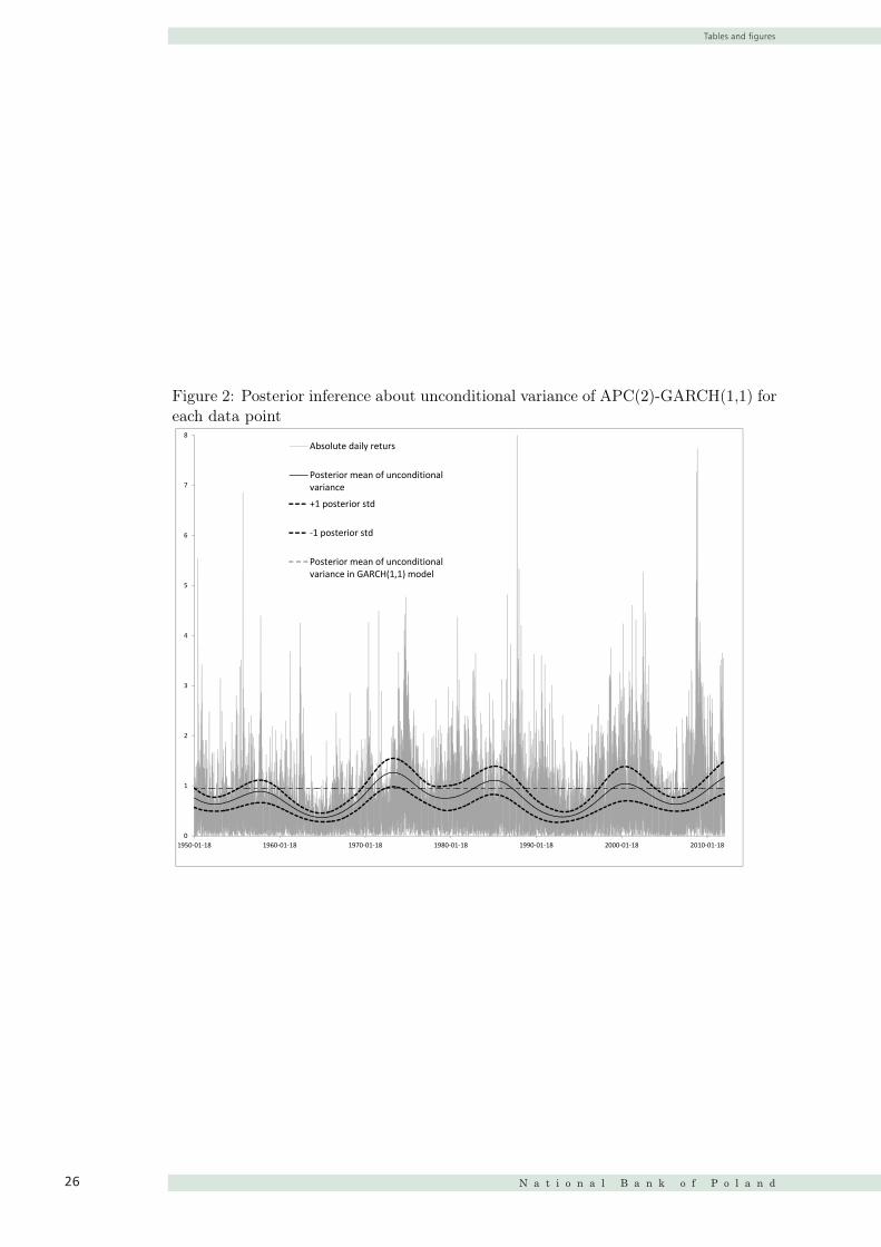
Tables and figur�es
N a t i o n a l B a n k o f P o l a n d26
Figure 2: Posterior inference about unconditional variance of APC(2)-GARCH(1,1) foreach data point
0
1
2
3
4
5
6
7
8
1950-01-18 1960-01-18 1970-01-18 1980-01-18 1990-01-18 2000-01-18 2010-01-18
Absolute daily returs
Posterior mean of unconditionalvariance
+1 posterior std
-1 posterior std
Posterior mean of unconditionalvariance in GARCH(1,1) model
26
Figure 3: Coexistence of changes in unconditional variance and recession periods forpostwar US economy marked by the National Bureau of Economic Research, NBER
0
0,5
1
1,5
2
2,5
3
-15
-10
-5
0
5
1950-01-18 1960-01-18 1970-01-18 1980-01-18 1990-01-18 2000-01-18 2010-01-18
Dataset Posterior mean of V(y_t)
+1 posterior std -1 posterior std
US Recessions (as marked by NBER)
27

Tables and figur�es
WORKING PAPER No. 124 27
Figure 2: Posterior inference about unconditional variance of APC(2)-GARCH(1,1) foreach data point
0
1
2
3
4
5
6
7
8
1950-01-18 1960-01-18 1970-01-18 1980-01-18 1990-01-18 2000-01-18 2010-01-18
Absolute daily returs
Posterior mean of unconditionalvariance
+1 posterior std
-1 posterior std
Posterior mean of unconditionalvariance in GARCH(1,1) model
26
Figure 3: Coexistence of changes in unconditional variance and recession periods forpostwar US economy marked by the National Bureau of Economic Research, NBER
0
0,5
1
1,5
2
2,5
3
-15
-10
-5
0
5
1950-01-18 1960-01-18 1970-01-18 1980-01-18 1990-01-18 2000-01-18 2010-01-18
Dataset Posterior mean of V(y_t)
+1 posterior std -1 posterior std
US Recessions (as marked by NBER)
27