national bank of poland working paper no. · pdf filenational bank of poland working paper no....
TRANSCRIPT

On asymmetric effects in a monetary policy rule. The case of Poland
Warsaw 2012
Anna Sznajderska
NATIONAL BANK OF POLANDWORKING PAPER
No. 125

Design:
Oliwka s.c.
Layout and print:
NBP Printshop
Published by:
National Bank of Poland Education and Publishing Department 00-919 Warszawa, 11/21 Świętokrzyska Street phone: +48 22 653 23 35, fax +48 22 653 13 21
© Copyright by the National Bank of Poland, 2012
ISSN 2084–624X
http://www.nbp.pl
Anna Sznajderska – National Bank of Poland; e-mail: [email protected]
I am grateful to Tomasz Łyziak and Ryszard Kokoszczyński for valuable comments and suggestions. The views expressed herein are those of the author and do not necessarily reflect those of the National Bank of Poland.
WORKING PAPER No. 125 1
Contents
Contents
Introduction 4
1 Literature review 6
1.1 Studies on the Taylor rule . . . . . . . . . . . . . . . . . . . . . . . . . . 61.2 Studies on the Phillips curve . . . . . . . . . . . . . . . . . . . . . . . . . 9
2 Data description 11
3 Methods of estimation and testing 13
3.1 The Phillips curve estimation . . . . . . . . . . . . . . . . . . . . . . . . 133.2 The Taylor rule estimation . . . . . . . . . . . . . . . . . . . . . . . . . . 143.3 The choice of the threshold value . . . . . . . . . . . . . . . . . . . . . . 15
4 Empirical results 17
4.1 A preliminary analysis of the nonlinear Philips curves . . . . . . . . . . . 174.2 The symmetric Taylor rules . . . . . . . . . . . . . . . . . . . . . . . . . 214.3 The asymmetric Taylor rules . . . . . . . . . . . . . . . . . . . . . . . . . 22
5 Concluding remarks 26
References 27
A Unit root tests 31
B Figures 32
2
3
5
5
8
10
12
12
13
14
16
16
20
21
25
26
30
31

Abstract
N a t i o n a l B a n k o f P o l a n d2
Abstract
Asymmetric effects in a monetary policy rule could appear due to asymmet-
ric preferences of the central bank or/and due to nonlinearities in the economic
system. It might be suspected that monetary authorities are more aggressive to
the inflation rate when it is above its target level than when it is below. It also
seems probable that monetary authorities have different preferences and react more
strongly when the level of economic activity is low than when it is high. In this
paper we investigate whether the reaction function of the National Bank of Poland
(NBP) is asymmetric according to the level of inflation gap and the level of output
gap. Moreover, we test whether these asymmetries might possibly stem from the
nonlinearities in the Phillips curve. Threshold models are applied and two cases of
unknown and known threshold value are investigated.
JEL Classification numbers: E52, E58, E30
Keywords: nonlinear Taylor rule, nonlinear Phillips curve, asymmetries, thresh-
old models
3
Introduction
The aim of this paper is to search for asymmetric effects in the reaction function ofthe National Bank of Poland (NBP). We check whether the Polish monetary policy ruleis asymmetric concerning levels of the fundamental macroeconomic variables: inflationand output gap. Encompassing the asymmetric elements in the reaction function mightgive better explanation of the central bank’s behavior. This, in turn, could help to formbetter expectations and forecasts and could be used to build more accurate econometricmodels of the economy.
If we assume that a central bank has quadratic loss function in the inflation andoutput gaps and minimizes it subject to linear structure of economy than we will obtaina linear reaction function. However, positive and negative deviations of inflation andoutput from the reference levels seem to be treated by monetary authorities differently.
On the one hand, central banks may have asymmetric preferences. Some centralbanks attempt to stabilize output fluctuations accepting inflation being more volatile,it is because they might face some political heat or social pressure. These banks wouldhave greater aversion to recessions than to expansions. Other central banks might befocused on inflation stabilization (e.g. strict inflation targeters) and have greater aversionto high than low inflation because, for instance, they need to build credibility afterimplementing inflation targeting strategy. Cukierman and Muscatelii (2008) distinguishrecession avoidance preferences (RAP) and inflation avoidance preferences (IAP). In theformer a central bank takes more precautions against negative output gaps, while inthe latter against positive inflation gaps. Such asymmetric preferences lead to nonlinearreaction functions, as the authors show RAP leads to concave Taylor rule while IAP toconvex rule in both the inflation and output gaps.
On the other hand, central banks might take into account asymmetries in differentchannels of the monetary transmission process. Most importantly, the aggregate supplycurve might be nonlinear. In empirical studies it is often argued that when the outputgap is positive it has positive impact on inflation, while when the output gap is negativeit has very small deflationary impact (Laxton et al. 1999, Pyyhtia 1999, Baghli et al.2006, Buchmann 2009). There are different explanations of this phenomenon, discussedlater on, such as for instance nominal wage rigidities, capacity constraints, costly priceadjustment, volatility of aggregate demand and supply shocks.
Lastly, the uncertainty regarding the NAIRU or the growth rate of productivity may
4

Introduction
WORKING PAPER No. 125 3
Abstract
Asymmetric effects in a monetary policy rule could appear due to asymmet-
ric preferences of the central bank or/and due to nonlinearities in the economic
system. It might be suspected that monetary authorities are more aggressive to
the inflation rate when it is above its target level than when it is below. It also
seems probable that monetary authorities have different preferences and react more
strongly when the level of economic activity is low than when it is high. In this
paper we investigate whether the reaction function of the National Bank of Poland
(NBP) is asymmetric according to the level of inflation gap and the level of output
gap. Moreover, we test whether these asymmetries might possibly stem from the
nonlinearities in the Phillips curve. Threshold models are applied and two cases of
unknown and known threshold value are investigated.
JEL Classification numbers: E52, E58, E30
Keywords: nonlinear Taylor rule, nonlinear Phillips curve, asymmetries, thresh-
old models
3
Introduction
The aim of this paper is to search for asymmetric effects in the reaction function ofthe National Bank of Poland (NBP). We check whether the Polish monetary policy ruleis asymmetric concerning levels of the fundamental macroeconomic variables: inflationand output gap. Encompassing the asymmetric elements in the reaction function mightgive better explanation of the central bank’s behavior. This, in turn, could help to formbetter expectations and forecasts and could be used to build more accurate econometricmodels of the economy.
If we assume that a central bank has quadratic loss function in the inflation andoutput gaps and minimizes it subject to linear structure of economy than we will obtaina linear reaction function. However, positive and negative deviations of inflation andoutput from the reference levels seem to be treated by monetary authorities differently.
On the one hand, central banks may have asymmetric preferences. Some centralbanks attempt to stabilize output fluctuations accepting inflation being more volatile,it is because they might face some political heat or social pressure. These banks wouldhave greater aversion to recessions than to expansions. Other central banks might befocused on inflation stabilization (e.g. strict inflation targeters) and have greater aversionto high than low inflation because, for instance, they need to build credibility afterimplementing inflation targeting strategy. Cukierman and Muscatelii (2008) distinguishrecession avoidance preferences (RAP) and inflation avoidance preferences (IAP). In theformer a central bank takes more precautions against negative output gaps, while inthe latter against positive inflation gaps. Such asymmetric preferences lead to nonlinearreaction functions, as the authors show RAP leads to concave Taylor rule while IAP toconvex rule in both the inflation and output gaps.
On the other hand, central banks might take into account asymmetries in differentchannels of the monetary transmission process. Most importantly, the aggregate supplycurve might be nonlinear. In empirical studies it is often argued that when the outputgap is positive it has positive impact on inflation, while when the output gap is negativeit has very small deflationary impact (Laxton et al. 1999, Pyyhtia 1999, Baghli et al.2006, Buchmann 2009). There are different explanations of this phenomenon, discussedlater on, such as for instance nominal wage rigidities, capacity constraints, costly priceadjustment, volatility of aggregate demand and supply shocks.
Lastly, the uncertainty regarding the NAIRU or the growth rate of productivity may
4

Introduction
N a t i o n a l B a n k o f P o l a n d4
lead to nonlinear interest rate policy as well (see Dolado et al. 2004). Therefore centralbanks might be more aggressive when the output gap reaches a certain threshold andmore cautious when the output gap is small.
The structure of this paper is as follows. In the next section a brief review of theliterature concerning symmetric Taylor rule and asymmetric effects in both Taylor ruleand Phillips curve is made. Section 2 and 3 present our data set and empirical strategy.Section 4 reports the empirical results. The last section concludes.
5
1 Literature review
1.1 Studies on the Taylor rule
Originally Taylor (1993) specified a simple monetary policy rule:
it = i∗ + πt + γyt + βπ(πt − π∗) = α + β(πt − π∗) + γyt,
where it is the central bank policy rate, i∗ is an equilibrium real interest rate, πt is therate of inflation over the previous four quarters, π∗ is the inflation target of the centralbank, yt is the percent deviation of the real GDP from its trend. Taylor (1993) analyzesthe federal funds rate during 1987-1992 and finds out that it is closely approximated bythe rule with parameters i∗ = 2, π∗ = 2, γ = βπ = 0, 5. Thus, the central bank ratetends to increase when the inflation is above its target value and when the actual outputis above the potential output.
The original Taylor rule has been modified in various ways. The adjustment of themonetary policy rate appears not to be immediate. Central banks dislike jumps and tendto smooth adjustments in their interest rates (Judd and Rudebusch (1998)). Therefore,the Taylor rule is often extended by a lagged interest rate term for instance as in theequation below (it is partial adjustment mechanism Clarida et al. 1998):
it = (1− ρ)(α + β(πt − π∗) + γyt) + ρit−1.
The central bank’s rate seems to depend on forecasts. The effects of the change of amonetary policy rate appear with delay1. If the monetary authorities take into accountthese delays than they should set their rates according to future movements of inflationand output gap. Clarida et al. (2000) suggest a following forward looking rule:
it = (1− ρ)(α + β(E(πt+k|Ωt)− π∗) + γE(yt+m|Ωt)) + ρit−1,
where Ωt denotes an information set at time t, yt+m is an output gap between period t
and t+m, πt+k is a percent change in a price level between periods t and t+ k.Moreover, many economists argue that standard monetary policy rules should be
augmented by other macroeconomic variables because central banks seem to look on thebroader set of factors. It is often proposed to extend the standard rule by: exchangerate, monetary aggregates, asset prices, long term and foreign interest rates. However,
1see Demchuk et al. (2012) for estimates for Poland
6

Literature review
WORKING PAPER No. 125 5
1
lead to nonlinear interest rate policy as well (see Dolado et al. 2004). Therefore centralbanks might be more aggressive when the output gap reaches a certain threshold andmore cautious when the output gap is small.
The structure of this paper is as follows. In the next section a brief review of theliterature concerning symmetric Taylor rule and asymmetric effects in both Taylor ruleand Phillips curve is made. Section 2 and 3 present our data set and empirical strategy.Section 4 reports the empirical results. The last section concludes.
5
1 Literature review
1.1 Studies on the Taylor rule
Originally Taylor (1993) specified a simple monetary policy rule:
it = i∗ + πt + γyt + βπ(πt − π∗) = α + β(πt − π∗) + γyt,
where it is the central bank policy rate, i∗ is an equilibrium real interest rate, πt is therate of inflation over the previous four quarters, π∗ is the inflation target of the centralbank, yt is the percent deviation of the real GDP from its trend. Taylor (1993) analyzesthe federal funds rate during 1987-1992 and finds out that it is closely approximated bythe rule with parameters i∗ = 2, π∗ = 2, γ = βπ = 0, 5. Thus, the central bank ratetends to increase when the inflation is above its target value and when the actual outputis above the potential output.
The original Taylor rule has been modified in various ways. The adjustment of themonetary policy rate appears not to be immediate. Central banks dislike jumps and tendto smooth adjustments in their interest rates (Judd and Rudebusch (1998)). Therefore,the Taylor rule is often extended by a lagged interest rate term for instance as in theequation below (it is partial adjustment mechanism Clarida et al. 1998):
it = (1− ρ)(α + β(πt − π∗) + γyt) + ρit−1.
The central bank’s rate seems to depend on forecasts. The effects of the change of amonetary policy rate appear with delay1. If the monetary authorities take into accountthese delays than they should set their rates according to future movements of inflationand output gap. Clarida et al. (2000) suggest a following forward looking rule:
it = (1− ρ)(α + β(E(πt+k|Ωt)− π∗) + γE(yt+m|Ωt)) + ρit−1,
where Ωt denotes an information set at time t, yt+m is an output gap between period t
and t+m, πt+k is a percent change in a price level between periods t and t+ k.Moreover, many economists argue that standard monetary policy rules should be
augmented by other macroeconomic variables because central banks seem to look on thebroader set of factors. It is often proposed to extend the standard rule by: exchangerate, monetary aggregates, asset prices, long term and foreign interest rates. However,
1see Demchuk et al. (2012) for estimates for Poland
6

Literature review
N a t i o n a l B a n k o f P o l a n d6
1
in the empirical studies these standard variables often seem to have negligible impact.More recently, for instance, Baxa et al. (2011) and Vašiček (2011), postulate to addsome measures of financial stability.
Furthermore Orphanides (2001, 2010) suggests to use real time data, which are avail-able to policymakers at the time of making the decision. The macroeconomic data suchas the rate of inflation or the level of GDP are known with the delay. The author arguesthat reliance on ex-post revised data can be misleading as the monetary authorities couldnot have actually followed such rule. The researcher can only imperfectly approximatethe real information available at time of making a policy decision.
Finally, many recent papers include threshold effects in a monetary policy reactionfunction. It is argued that the linear specifications can be too simplified. Such approach,also applied in our paper, enables to encompass an asymmetric behavior of central banks.
Bunzel and Enders (2010) find out strong evidence of threshold behaviour of theFederal Reserve in a number of time periods between 1965 and 2007. Among othersthe authors present model where the central bank is active when the inflation is higherthan the interim threshold and when the output gap is negative. It appears that thecentral bank is more aggressive when the system is above the threshold than when it isbelow. The model seems to fit data best, what is more, the models with asymmetriceffects give better out-of-sample forecasts than the linear models. But, the authors noticealso a number of statistical problems that might arise while analysing the asymmetriesand result in quite dubious results. For example, the threshold value and Hansen’sF statistic decrease when increasing the starting date, moreover, in the high inflationregime excessive amount of interest rate smoothing may be observed.
Cukierman and Muscatelli (2008) using smooth transition regressions study nonlin-earities in the monetary policy rule for the UK and the US. They emphasize that thecharacter of nonlinearities changes substantially over different time periods and dependsmainly on the regime and the macroeconomic situation. For instance in the 1979 - 1990in the UK the Taylor rule seems to be concave, what can be interpreted as dominanceof recession avoidance preferences, whereas in the 1992-2005 it appears to be convex,what might be interpreted as dominance of inflation avoidance preferences. The similarfindings are presented for the US - where the Taylor rule varies across different chair-men of the Fed - inflation avoidance preference dominated under Martin and recessionavoidance preference during Burns/Miller and Greenspan.
The asymmetric effects in European Central Bank (ECB) reaction function were
7
studied by many researchers. Aguiar and Martins (2008) point out that when a centralbank needs to build credibility than it would be more precautionary as far as a pricestability is concerned. Therefore, it would prefer to have inflation below the target levelthan above. Such asymmetry is shown for the Euro Area throughout 1995 - 2005, asduring this time period the monetary policy had to establish its credibility. WhereasSurico (2003) estimates the asymmetric Taylor rule for ECB concerning the sample1997:7 - 2002:10 and finds equal reaction to inflation and deflation, but larger policyeasing during output recessions than policy tightening during output expansions. Inone of the recent papers Gerlach and Lewis (2011) estimate the ECB’s monetary policyrule in 1999-2010 and detect a structural break after November 2008 (i.e. the switchingpoint). Interestingly, they use smooth transition model to avoid a discrete break. Theauthors focus on the recent financial crisis and show that the zero lower bound did notconstrain monetary policy during the crisis.
As far as the Polish monetary rule is concerned a few studies were conducted. Ur-bańska (2002) presents one of the first attempt to estimate the Polish Taylor rule.She concerns the period 03:1998 - 12:2001 and uses the error correction model (ECM).Kotłowski (2006) analyses the individual reaction functions of MPC members in 2004-2005. Przystupa and Wróbel (2006) estimate small structural model with different de-grees of forward-lookingness and calculate loss functions to determine the optimal mone-tary policy rule. Whereas Baranowski (2008) uses real time data to estimate by the ECMbackward looking Taylor rule in Q1:1999 - Q3:2007. Moreover, Brzoza - Brzezina et al.(2011) try to determine the extent to which the three chosen central banks (i.e. Bank ofEngland, National Bank of Poland and Swiss National Bank) are forward-looking.
The Taylor rule might be asymmetric because of some asymmetric effects in themonetary transmission mechanism. Here’s a brief presentation of the studies for thePolish economy. Postek (2011) presents the 3-equation nonlinear model. The resultsindicate the following asymmetric effects: a negative relation between the GDP dynamicsin the current year and in the previous year if the change of the dynamics reaches acertain level, higher persistence of the increasing or stable inflation than the decreasingone, and stronger reaction of the NBP’s reference rate in response to the rapid decreaseof inflation than to its rapid increase. Łyziak et. al (2010) apply a small structural modelwith nonlinear Phillips curve where the impact of the output gap on inflation is strongerwhen the output gap is positive. Concerning the particular channels of the monetarytransmission, Przystupa and Wróbel (2009) study an exchange rate pass-through and
8

Literature review
WORKING PAPER No. 125 7
1
in the empirical studies these standard variables often seem to have negligible impact.More recently, for instance, Baxa et al. (2011) and Vašiček (2011), postulate to addsome measures of financial stability.
Furthermore Orphanides (2001, 2010) suggests to use real time data, which are avail-able to policymakers at the time of making the decision. The macroeconomic data suchas the rate of inflation or the level of GDP are known with the delay. The author arguesthat reliance on ex-post revised data can be misleading as the monetary authorities couldnot have actually followed such rule. The researcher can only imperfectly approximatethe real information available at time of making a policy decision.
Finally, many recent papers include threshold effects in a monetary policy reactionfunction. It is argued that the linear specifications can be too simplified. Such approach,also applied in our paper, enables to encompass an asymmetric behavior of central banks.
Bunzel and Enders (2010) find out strong evidence of threshold behaviour of theFederal Reserve in a number of time periods between 1965 and 2007. Among othersthe authors present model where the central bank is active when the inflation is higherthan the interim threshold and when the output gap is negative. It appears that thecentral bank is more aggressive when the system is above the threshold than when it isbelow. The model seems to fit data best, what is more, the models with asymmetriceffects give better out-of-sample forecasts than the linear models. But, the authors noticealso a number of statistical problems that might arise while analysing the asymmetriesand result in quite dubious results. For example, the threshold value and Hansen’sF statistic decrease when increasing the starting date, moreover, in the high inflationregime excessive amount of interest rate smoothing may be observed.
Cukierman and Muscatelli (2008) using smooth transition regressions study nonlin-earities in the monetary policy rule for the UK and the US. They emphasize that thecharacter of nonlinearities changes substantially over different time periods and dependsmainly on the regime and the macroeconomic situation. For instance in the 1979 - 1990in the UK the Taylor rule seems to be concave, what can be interpreted as dominanceof recession avoidance preferences, whereas in the 1992-2005 it appears to be convex,what might be interpreted as dominance of inflation avoidance preferences. The similarfindings are presented for the US - where the Taylor rule varies across different chair-men of the Fed - inflation avoidance preference dominated under Martin and recessionavoidance preference during Burns/Miller and Greenspan.
The asymmetric effects in European Central Bank (ECB) reaction function were
7
studied by many researchers. Aguiar and Martins (2008) point out that when a centralbank needs to build credibility than it would be more precautionary as far as a pricestability is concerned. Therefore, it would prefer to have inflation below the target levelthan above. Such asymmetry is shown for the Euro Area throughout 1995 - 2005, asduring this time period the monetary policy had to establish its credibility. WhereasSurico (2003) estimates the asymmetric Taylor rule for ECB concerning the sample1997:7 - 2002:10 and finds equal reaction to inflation and deflation, but larger policyeasing during output recessions than policy tightening during output expansions. Inone of the recent papers Gerlach and Lewis (2011) estimate the ECB’s monetary policyrule in 1999-2010 and detect a structural break after November 2008 (i.e. the switchingpoint). Interestingly, they use smooth transition model to avoid a discrete break. Theauthors focus on the recent financial crisis and show that the zero lower bound did notconstrain monetary policy during the crisis.
As far as the Polish monetary rule is concerned a few studies were conducted. Ur-bańska (2002) presents one of the first attempt to estimate the Polish Taylor rule.She concerns the period 03:1998 - 12:2001 and uses the error correction model (ECM).Kotłowski (2006) analyses the individual reaction functions of MPC members in 2004-2005. Przystupa and Wróbel (2006) estimate small structural model with different de-grees of forward-lookingness and calculate loss functions to determine the optimal mone-tary policy rule. Whereas Baranowski (2008) uses real time data to estimate by the ECMbackward looking Taylor rule in Q1:1999 - Q3:2007. Moreover, Brzoza - Brzezina et al.(2011) try to determine the extent to which the three chosen central banks (i.e. Bank ofEngland, National Bank of Poland and Swiss National Bank) are forward-looking.
The Taylor rule might be asymmetric because of some asymmetric effects in themonetary transmission mechanism. Here’s a brief presentation of the studies for thePolish economy. Postek (2011) presents the 3-equation nonlinear model. The resultsindicate the following asymmetric effects: a negative relation between the GDP dynamicsin the current year and in the previous year if the change of the dynamics reaches acertain level, higher persistence of the increasing or stable inflation than the decreasingone, and stronger reaction of the NBP’s reference rate in response to the rapid decreaseof inflation than to its rapid increase. Łyziak et. al (2010) apply a small structural modelwith nonlinear Phillips curve where the impact of the output gap on inflation is strongerwhen the output gap is positive. Concerning the particular channels of the monetarytransmission, Przystupa and Wróbel (2009) study an exchange rate pass-through and
8

Literature review
N a t i o n a l B a n k o f P o l a n d8
1
find an asymmetry of CPI reaction to the output gap and exchange rate movements (i.e.the size and direction of the exchange rate change, and volatility of the exchange rate).Whereas Sznajderska (2012) examines an interest rate pass-through and, for certainretail bank interest rates, finds evidence of asymmetric cointegration and short termasymmetric effects concerning the levels of economic activity and liquidity.
Vašiček (2011) concerns the asymmetric effects in the Polish monetary policy rule.The author investigates the Taylor rules for the Czech Republic, Hungary and Polandand searches for asymmetries assigned to the level of inflation, output gap and financialstress. Our approach is in some cases similar to this paper, however, our results arevery different. Vašiček does not find nonlinearities in the Polish Philips curve and whatis more he finds little evidence of any linear or nonlinear relationship between inflationand stance of business cycle. The author finds out that the Polish central bank respondsrather to the output gap than inflation. There are no asymmetries in the Taylor rule asfar as the level of inflation is concerned. Moreover, the analysis shows that NBP seems tobe asymmetric along the business cycle as the output gap coefficient is insignificant in theregime below the threshold value and significant above it. The author’s interpretationis that the output gap affects NBP’s inflation forecasts which are the driver of interestrate setting. In addition, the calculations show that when financial stress is high there isno response to inflation and when it is low the response is positive. The author suggeststhat the real economy raises concerns only when the inflation stress is low.
1.2 Studies on the Phillips curve
As it was mentioned before a nonlinear monetary policy reaction function might stemfrom nonlinear Philips curve. The Phillips curve has generally been estimated in a linearframework2, even though the original work of Phillips (1958) and many other theoreticalworks pointed to nonlinear relationship.
Many economists argue that the relation between inflation and output gap is non-linear, therefore the cost of disinflation is changing. Often the Phillips curve seems tobe convex. If the economy is overheated an decrease of economic activity causes fasterdisinflation (cost of fighting inflation is low), while in the contrary when the economy isin recession further decreases of economic activity do not cause much disinflation (costof fighting inflation is high).
2However, the studies mainly concerned the neutrality of money in short and long term and theexistence of the relation between economic activity and inflation at all.
9
There are many reasons for the nonlinear Phillips curve. For instance, workers areresistant to nominal wage cuts, what causes downward rigidity of nominal wages. It isparticularly problematic when the level of inflation is low, because when the inflation rateis high it might be enough to keep the nominal wages constant for some time to decreasethe wages. Thus, the central bank to restore the balance on the labor market mighttolerate higher inflation. Even long run Philips curve might be down-sloping (in theinflation-unemployment space) because of money illusion (Akerlof et al., 1996), peopleuse to think in nominal terms, therefore in a period of high inflation firms can set lowerreal wages and hire more workers.
Moreover, firms may face capacity constraints in the short run. When the economyis strong the capacity constraints restrict firms to increase output and encourage themto increase prices, in contrast when the economy is weak it is easier for firms to increaseoutput, what causes a convex Philips curve.
Costly price adjustment (Ball et al. 1988, Dotsey et al. 1999) are another explanation.Any change in firms’ activity is costly, therefore firms might be reluctant to make it.When the level of inflation is high demand shock is expected to have more impact onincreasing prices and less on increasing production.
Also volatility of aggregate demand and supply shocks (Lucas 1973) might causesome asymmetric effects. Economic entities do not know if any price change is causedby a change in the economy wide aggregate demand or by a change in relative productdemand and thus, they are unable to distinguish between changes in general prices andchanges in relative prices. The higher the volatility of inflation the more of price changesare assigned to general prices. Therefore, not only the level of inflation but also itsstability is an important aspect for monetary authorities.
There are not only studies which show that the Philips curve is convex, some studiespoint that it might be concave. It might be concave because firms facing monopolisticcompetition are more willing to reduce prices under weak demand (when the output gapis negative) than to increase them under high demand to avoid being overtaken by rivalfirms (Stiglitz, 1997).
Filardo (1998) point out that the Philips curve might be convex when the outputgap is positive and concave when the output gap is negative. The author shows that thecost of fighting inflation is higher when the economy is weak (5% of output gap) thanwhen it is overheated (2, 1%). Moreover, in both the weak and the overheated economythis cost is higher than it results from the linear model.
10
Literature review
WORKING PAPER No. 125 9
1
find an asymmetry of CPI reaction to the output gap and exchange rate movements (i.e.the size and direction of the exchange rate change, and volatility of the exchange rate).Whereas Sznajderska (2012) examines an interest rate pass-through and, for certainretail bank interest rates, finds evidence of asymmetric cointegration and short termasymmetric effects concerning the levels of economic activity and liquidity.
Vašiček (2011) concerns the asymmetric effects in the Polish monetary policy rule.The author investigates the Taylor rules for the Czech Republic, Hungary and Polandand searches for asymmetries assigned to the level of inflation, output gap and financialstress. Our approach is in some cases similar to this paper, however, our results arevery different. Vašiček does not find nonlinearities in the Polish Philips curve and whatis more he finds little evidence of any linear or nonlinear relationship between inflationand stance of business cycle. The author finds out that the Polish central bank respondsrather to the output gap than inflation. There are no asymmetries in the Taylor rule asfar as the level of inflation is concerned. Moreover, the analysis shows that NBP seems tobe asymmetric along the business cycle as the output gap coefficient is insignificant in theregime below the threshold value and significant above it. The author’s interpretationis that the output gap affects NBP’s inflation forecasts which are the driver of interestrate setting. In addition, the calculations show that when financial stress is high there isno response to inflation and when it is low the response is positive. The author suggeststhat the real economy raises concerns only when the inflation stress is low.
1.2 Studies on the Phillips curve
As it was mentioned before a nonlinear monetary policy reaction function might stemfrom nonlinear Philips curve. The Phillips curve has generally been estimated in a linearframework2, even though the original work of Phillips (1958) and many other theoreticalworks pointed to nonlinear relationship.
Many economists argue that the relation between inflation and output gap is non-linear, therefore the cost of disinflation is changing. Often the Phillips curve seems tobe convex. If the economy is overheated an decrease of economic activity causes fasterdisinflation (cost of fighting inflation is low), while in the contrary when the economy isin recession further decreases of economic activity do not cause much disinflation (costof fighting inflation is high).
2However, the studies mainly concerned the neutrality of money in short and long term and theexistence of the relation between economic activity and inflation at all.
9
There are many reasons for the nonlinear Phillips curve. For instance, workers areresistant to nominal wage cuts, what causes downward rigidity of nominal wages. It isparticularly problematic when the level of inflation is low, because when the inflation rateis high it might be enough to keep the nominal wages constant for some time to decreasethe wages. Thus, the central bank to restore the balance on the labor market mighttolerate higher inflation. Even long run Philips curve might be down-sloping (in theinflation-unemployment space) because of money illusion (Akerlof et al., 1996), peopleuse to think in nominal terms, therefore in a period of high inflation firms can set lowerreal wages and hire more workers.
Moreover, firms may face capacity constraints in the short run. When the economyis strong the capacity constraints restrict firms to increase output and encourage themto increase prices, in contrast when the economy is weak it is easier for firms to increaseoutput, what causes a convex Philips curve.
Costly price adjustment (Ball et al. 1988, Dotsey et al. 1999) are another explanation.Any change in firms’ activity is costly, therefore firms might be reluctant to make it.When the level of inflation is high demand shock is expected to have more impact onincreasing prices and less on increasing production.
Also volatility of aggregate demand and supply shocks (Lucas 1973) might causesome asymmetric effects. Economic entities do not know if any price change is causedby a change in the economy wide aggregate demand or by a change in relative productdemand and thus, they are unable to distinguish between changes in general prices andchanges in relative prices. The higher the volatility of inflation the more of price changesare assigned to general prices. Therefore, not only the level of inflation but also itsstability is an important aspect for monetary authorities.
There are not only studies which show that the Philips curve is convex, some studiespoint that it might be concave. It might be concave because firms facing monopolisticcompetition are more willing to reduce prices under weak demand (when the output gapis negative) than to increase them under high demand to avoid being overtaken by rivalfirms (Stiglitz, 1997).
Filardo (1998) point out that the Philips curve might be convex when the outputgap is positive and concave when the output gap is negative. The author shows that thecost of fighting inflation is higher when the economy is weak (5% of output gap) thanwhen it is overheated (2, 1%). Moreover, in both the weak and the overheated economythis cost is higher than it results from the linear model.
10

Data description
N a t i o n a l B a n k o f P o l a n d10
2
2 Data description
We use monthly publicly available data from January 2000 to May 2012. On the onehand usage of monthly data enables us to apply threshold models and have sufficientnumber of observations while on the other hand interest rates and inflation rates arehighly persistent at monthly frequencies what might result in the coefficient of laggeddependent variable close to unity and very limited response of independent variables.
In the case of a monetary policy rule estimation an important aspect of the dataselection process is determining the dependent variable. The Polish monetary policyrate is usually adjusted by multiples of 25 basis points and the decisions concerningits level are taken once a month. Taking into account this discreteness we decided toconcentrate on the money market rate, which is more variable and determines the realrate of making transactions. The Polish central bank reference rate and the moneymarket rates move almost in line during the examined time period (see Figure 1). In thestudy we will use the 1 week money market rate - WIBOR 1W as dependent variable.
All data are obtain from the webpage of the Polish Central Statistical Office or theNational Bank of Poland database. Let as denote the other time series used in theestimations:
• cpi1 - year on year consumer price index;
• cpi2 - quarter on quarter consumer price index, seasonally adjusted;
• cpia - the deviation of cpi from the actual inflation target;
• cpib - the deviation of cpi from its smoothed by Hodrick Prescott filter trend ofinflation (i.e. cpi1);
• gap - the difference between logarithm of the seasonally adjusted measure of GDPand the trend obtained by Hodrick Prescott filter, GDP is disaggregated to monthlyfrequencies; We use Fernandez method to disaggregate quarterly data into monthlyfrequencies (cf. Fernandez, 1981). We use an output gap computed for monthlyindustrial production index to augment the related series. Moreover, we lengthenthe time series by AR(2) process to diminish the role of last observations.
• reer - difference between logarithm of real effective exchange rate deflated by CPI(which is calculated by the National Bank of Poland) and the trend obtained byHodrick Prescott filter;
11
• infe1 - inflation expectations of Polish bank analysts for forecasting horizon of 12months from the survey conducted by Reuters;
• infe2 - inflation expectations of Polish consumers for forecasting horizon of 12months, calculated from the survey conducted by Ipsos (cf. Łyziak and Stanisławska2006);
• ∆ieuro - the change of 1 month EURIBOR.
The graphs of the applied variables are presented in Figure 1 in the Appendix.Belke and Klose (2011) argue that different regression coefficients can be obtained
when using ex-post data, real-time data and non-modified real-time forecasts. Theyestimate the ECB response function in period 1999Q1 - 2010Q2 and find out that higherinflation and output gap coefficients are obtained when one uses real time data insteadof ex-post data, moreover the output gap coefficient is reduced when one uses real timeforecasts. However, we do not use the data from projections of inflation and GDP becausethey are publicly available since 08:2004 and 05:2005 respectively. Moreover, these arequarterly not monthly data.
12

Data description
WORKING PAPER No. 125 11
2
2 Data description
We use monthly publicly available data from January 2000 to May 2012. On the onehand usage of monthly data enables us to apply threshold models and have sufficientnumber of observations while on the other hand interest rates and inflation rates arehighly persistent at monthly frequencies what might result in the coefficient of laggeddependent variable close to unity and very limited response of independent variables.
In the case of a monetary policy rule estimation an important aspect of the dataselection process is determining the dependent variable. The Polish monetary policyrate is usually adjusted by multiples of 25 basis points and the decisions concerningits level are taken once a month. Taking into account this discreteness we decided toconcentrate on the money market rate, which is more variable and determines the realrate of making transactions. The Polish central bank reference rate and the moneymarket rates move almost in line during the examined time period (see Figure 1). In thestudy we will use the 1 week money market rate - WIBOR 1W as dependent variable.
All data are obtain from the webpage of the Polish Central Statistical Office or theNational Bank of Poland database. Let as denote the other time series used in theestimations:
• cpi1 - year on year consumer price index;
• cpi2 - quarter on quarter consumer price index, seasonally adjusted;
• cpia - the deviation of cpi from the actual inflation target;
• cpib - the deviation of cpi from its smoothed by Hodrick Prescott filter trend ofinflation (i.e. cpi1);
• gap - the difference between logarithm of the seasonally adjusted measure of GDPand the trend obtained by Hodrick Prescott filter, GDP is disaggregated to monthlyfrequencies; We use Fernandez method to disaggregate quarterly data into monthlyfrequencies (cf. Fernandez, 1981). We use an output gap computed for monthlyindustrial production index to augment the related series. Moreover, we lengthenthe time series by AR(2) process to diminish the role of last observations.
• reer - difference between logarithm of real effective exchange rate deflated by CPI(which is calculated by the National Bank of Poland) and the trend obtained byHodrick Prescott filter;
11
• infe1 - inflation expectations of Polish bank analysts for forecasting horizon of 12months from the survey conducted by Reuters;
• infe2 - inflation expectations of Polish consumers for forecasting horizon of 12months, calculated from the survey conducted by Ipsos (cf. Łyziak and Stanisławska2006);
• ∆ieuro - the change of 1 month EURIBOR.
The graphs of the applied variables are presented in Figure 1 in the Appendix.Belke and Klose (2011) argue that different regression coefficients can be obtained
when using ex-post data, real-time data and non-modified real-time forecasts. Theyestimate the ECB response function in period 1999Q1 - 2010Q2 and find out that higherinflation and output gap coefficients are obtained when one uses real time data insteadof ex-post data, moreover the output gap coefficient is reduced when one uses real timeforecasts. However, we do not use the data from projections of inflation and GDP becausethey are publicly available since 08:2004 and 05:2005 respectively. Moreover, these arequarterly not monthly data.
12

Methods of estimation and testing
N a t i o n a l B a n k o f P o l a n d12
3
3 Methods of estimation and testing
3.1 The Phillips curve estimation
Before proceeding with the analysis of the Taylor rule we examine nonlinearities inthe Polish Philips curve. We do only a preliminary analysis and further studies areneeded when using different measures of inflation and output gap as well as differentspecifications of the Philips curve. As the main aim of this paper is to analyse possibleasymmetries in the Taylor rule, the estimations of the Phillips curve aim to show ifthe asymmetries in the Taylor rule might stem from the nonlinear relation between theinflation rate and the level of economic activity. Therefore, to obtain comparable resultswe use similar data in both the Phillips curve and the Taylor rule estimations. It meansthat when estimating the Philips curve we consider monthly data. We consider twomeasures of inflation: year on year CPI as the central bank target is maintaining thisrate at the relevant level and quarter on quarter CPI as such rate is most often used andenables better economic explanation from independent variables to CPI.
We use GMM estimation method with lagged values of the measure of inflation,output gap, exchange rate gap and inflation expectations of the Polish customers andbank analysts as instruments.
We estimate the New Keynesian hybrid Phillips curve with forward and backwardlooking components of expected price movements, output gap and exchange rate pass-through:
πt = λ1E(πt+k|Ωt) + λ2πt−k + αyt−n + φet−m + ε, (1)
where: πt is an inflation rate measured by cpi1 or cpi2, yt is an output gap measuredby gap, et is an exchange rate gap measured by reer. Ωt in this and other equationsdenotes an information set at time t. Various combinations of the lead and lag values(i.e. k, n,m) will be tested, where k, n,m ∈ 3, 4, . . . , 12 and the model which fits thedata best will be chosen.
Next, the asymmetries concerning the level of output gap are tested in the twofollowing ways:
πt = (λ11E(πt+k|Ωt) + λ21πt−k + α1yt−n + φ1et−m)It + (2)
+(λ12E(πt+k|Ωt) + λ22πt−k + α2yt−n + φ2et−m)(1− It) + ε,
πt = λ1E(πt+k|Ωt) + λ2πt−k + α1yt−nIt + α2yt−n(1− It) + φet−m + ε, (3)
13
where:
It =
1 if yt−n ≥ τ ,
0 otherwise.
In the Equation (2) we concern the case when the whole Phillips curve rule changesaccording to the value of the threshold variable. Whereas in the Equation (3) we concernthe case when only the coefficients of the output gap change depending on the value ofa known threshold value. The way in which the threshold values (τ) are obtained ispresented in Section 4.3.
Dolado et al. (2004)3 show that when the Philips curve is nonlinear (convex orconcave) than the Taylor rule resembles a linear one but it is extended by the interactionterm of expected inflation and the output gap. For example when a Phillips curve isconvex, an expected inflation caused by a higher output gap will be larger than in alinear specification, so anticipating this policy makers will react more forcefully (whatis captured by the interaction term). Thus, additionally, we perform a similar test toDolado et al. (2004) and we try to include a nonlinear component yt−nyt−n. We testwhether the additional component is statistically significant in the following equation:
πt = λ1E(πt+k|Ωt) + λ2πt−k + αyt−n + α1yt−nyt−n + φet−m + ε. (4)
3.2 The Taylor rule estimation
We then turn to an analysis of the Polish Taylor rule. We consider two models withtwo different measures of inflation target (cpia and cpib) to check the robustness of theresults.
As previously, to allow for correlation between the error term and the forward lookingvariables, we use GMM method with instruments such as lagged values of the inflationgap, the output gap, the domestic short term interest rate as well as the short terminterest rate in the euro area, and the real effective exchange rate.
Firstly, we estimate the symmetric Taylor rule as in the following equation:
it = ρit−1 + βE(πt+h − π∗t+h|Ωt) + γE(yt+l|Ωt) + α, (5)
where: it is the one week Polish money market rate (Wibor 1W), π∗ is an inflation target,measured as the actual inflation target (cpia) or the smoothed by Hodrick Prescott
3Dolado et al. (2004), concerning the central banks of Germany, France, Spain, the US and Euroarea, find out that the Philips curve is convex in all cases except the US.
14

Methods of estimation and testing
WORKING PAPER No. 125 13
3
3 Methods of estimation and testing
3.1 The Phillips curve estimation
Before proceeding with the analysis of the Taylor rule we examine nonlinearities inthe Polish Philips curve. We do only a preliminary analysis and further studies areneeded when using different measures of inflation and output gap as well as differentspecifications of the Philips curve. As the main aim of this paper is to analyse possibleasymmetries in the Taylor rule, the estimations of the Phillips curve aim to show ifthe asymmetries in the Taylor rule might stem from the nonlinear relation between theinflation rate and the level of economic activity. Therefore, to obtain comparable resultswe use similar data in both the Phillips curve and the Taylor rule estimations. It meansthat when estimating the Philips curve we consider monthly data. We consider twomeasures of inflation: year on year CPI as the central bank target is maintaining thisrate at the relevant level and quarter on quarter CPI as such rate is most often used andenables better economic explanation from independent variables to CPI.
We use GMM estimation method with lagged values of the measure of inflation,output gap, exchange rate gap and inflation expectations of the Polish customers andbank analysts as instruments.
We estimate the New Keynesian hybrid Phillips curve with forward and backwardlooking components of expected price movements, output gap and exchange rate pass-through:
πt = λ1E(πt+k|Ωt) + λ2πt−k + αyt−n + φet−m + ε, (1)
where: πt is an inflation rate measured by cpi1 or cpi2, yt is an output gap measuredby gap, et is an exchange rate gap measured by reer. Ωt in this and other equationsdenotes an information set at time t. Various combinations of the lead and lag values(i.e. k, n,m) will be tested, where k, n,m ∈ 3, 4, . . . , 12 and the model which fits thedata best will be chosen.
Next, the asymmetries concerning the level of output gap are tested in the twofollowing ways:
πt = (λ11E(πt+k|Ωt) + λ21πt−k + α1yt−n + φ1et−m)It + (2)
+(λ12E(πt+k|Ωt) + λ22πt−k + α2yt−n + φ2et−m)(1− It) + ε,
πt = λ1E(πt+k|Ωt) + λ2πt−k + α1yt−nIt + α2yt−n(1− It) + φet−m + ε, (3)
13
where:
It =
1 if yt−n ≥ τ ,
0 otherwise.
In the Equation (2) we concern the case when the whole Phillips curve rule changesaccording to the value of the threshold variable. Whereas in the Equation (3) we concernthe case when only the coefficients of the output gap change depending on the value ofa known threshold value. The way in which the threshold values (τ) are obtained ispresented in Section 4.3.
Dolado et al. (2004)3 show that when the Philips curve is nonlinear (convex orconcave) than the Taylor rule resembles a linear one but it is extended by the interactionterm of expected inflation and the output gap. For example when a Phillips curve isconvex, an expected inflation caused by a higher output gap will be larger than in alinear specification, so anticipating this policy makers will react more forcefully (whatis captured by the interaction term). Thus, additionally, we perform a similar test toDolado et al. (2004) and we try to include a nonlinear component yt−nyt−n. We testwhether the additional component is statistically significant in the following equation:
πt = λ1E(πt+k|Ωt) + λ2πt−k + αyt−n + α1yt−nyt−n + φet−m + ε. (4)
3.2 The Taylor rule estimation
We then turn to an analysis of the Polish Taylor rule. We consider two models withtwo different measures of inflation target (cpia and cpib) to check the robustness of theresults.
As previously, to allow for correlation between the error term and the forward lookingvariables, we use GMM method with instruments such as lagged values of the inflationgap, the output gap, the domestic short term interest rate as well as the short terminterest rate in the euro area, and the real effective exchange rate.
Firstly, we estimate the symmetric Taylor rule as in the following equation:
it = ρit−1 + βE(πt+h − π∗t+h|Ωt) + γE(yt+l|Ωt) + α, (5)
where: it is the one week Polish money market rate (Wibor 1W), π∗ is an inflation target,measured as the actual inflation target (cpia) or the smoothed by Hodrick Prescott
3Dolado et al. (2004), concerning the central banks of Germany, France, Spain, the US and Euroarea, find out that the Philips curve is convex in all cases except the US.
14
Methods of estimation and testing
N a t i o n a l B a n k o f P o l a n d14
3
filter trend of actual inflation (cpib), yt is the output gap. We choose the lead valuesh ∈ 3, 4, . . . , 12 and l ∈ 0, 1, . . . , 3 which fit the model best.
Next, we estimate the asymmetric Taylor rules. Namely, we estimate the thresholdmodel for the Polish monetary reaction function as:
it =(ρ1it−1 + β1E(πt+h − π∗
t+h|Ωt) + γ1E(yt+l|Ωt) + α1
)It + (6)
+(ρ2it−1 + β2E(πt+h − π∗
t+h|Ωt) + γ2E(yt+l|Ωt) + α2
)(1− It) + εt,
it = ρit−1 + β1E(πt+h − π∗t+h|Ωt)It+h + γ1E(yt+l|Ωt)Jt+l + (7)
+ β2E(πt+h − π∗t+h|Ωt)(1− It+h) + γ2E(yt+l|Ωt)(1− Jt+l) + α + εt,
where
It =
1 if mt ≥ τ1,
0 otherwise,Jt =
1 if nt ≥ τ2,
0 otherwise,
and mt and nt are the threshold variables in period t, in our case it is the inflation gapor the output gap. As far as the Equation (7) is concerned we consider the case wheremt = nt and mt denotes the inflation gap and nt denotes the output gap. It means thatthe central bank responds asymmetrically to the level of inflation gap depending on thevalue of inflation gap but not depending on the value of the output gap and opposite, inthe same time the central bank responds asymmetrically to the level of the output gapdepending on the value of the output gap but not depending on the value of the inflationgap. We consider also the case when Jt = 1 for each t and mt is an inflation gap, thatis an asymmetry according only to the inflation gap, and the case when It = 1 for eacht and nt is an output gap, that is the asymmetry according only to the level of outputgap.
3.3 The choice of the threshold value
In both the estimations of the Taylor rule and the Phillips curve we consider two casesof known and unknown threshold values. In case of unknown parameter we estimatethe threshold value using the procedure presented in Caner and Hansen (2004). Thethreshold value is the one that minimizes the sum of the square errors (Sn) of the 2SLSestimation, i.e.:
τ = argminτ∈ΓSn(τ).
15
We draw the LR-like statistics:
LRn(τ) = nSn(τ)− Sn(τ)
Sn(τ). (8)
The shape of this statistic indicates the strength of the threshold effect. When theLR statistic line has a clearly defined minimum (a V-shaped line) it means that thethreshold effect is strong. Whereas, when it has irregular shape it is an indication ofweaker threshold effects. The critical value cuts off the interval of all possible thresholdvalues.
We compute the Sup test proposed by Caner and Hansen (2004). This test is oftenused to test the presence of threshold effects (see Bunzel and Enders (2010) or Mandler(2011)). To do so we estimate by GMM the Equation (2) or (6), respectively, for a fixedvalue τ ∈ Γ. Then we calculate the Wald statistic for H0 : ρ1 = ρ2, α1 = α2, β1 =
β2, γ1 = γ2, we denote it by Wn(τ). We repeat this calculation for all τ ∈ Γ andthe Sup statistic is then the largest value of these statistics, SupW = supτ∈ΓWn(τ).The asymptotic distribution of this statistic is not chi-square as the parameter τ is notidentified under the null hypothesis. Therefore, we need to calculate it by simulation(so-called bootstrapping). We define pseudodependent variable εt(τ)ηt where εt(τ) is theerror term for the Equation (2) or (6) and ηt is i.i.d. N(0, 1). We repeat the calculationsfor the pseudodependent variable in place of it for the unrestricted model. The resultingstatistic SupW ∗ has the needed asymptotic distribution.
In the case of known threshold parameter we use the chosen quantiles of the outputgap or inflation gap. For the Phillips curve it is τ = 0 or τ = 0,7 quantile of the measureof the output gap, which correspond to the regimes of positive and negative output gapand the regime of very high output gap. For the Taylor rule these are medians of thethe measures of output gap and inflation gap, which divide the sample into two equalsubsamples.
16

Methods of estimation and testing
WORKING PAPER No. 125 15
3
filter trend of actual inflation (cpib), yt is the output gap. We choose the lead valuesh ∈ 3, 4, . . . , 12 and l ∈ 0, 1, . . . , 3 which fit the model best.
Next, we estimate the asymmetric Taylor rules. Namely, we estimate the thresholdmodel for the Polish monetary reaction function as:
it =(ρ1it−1 + β1E(πt+h − π∗
t+h|Ωt) + γ1E(yt+l|Ωt) + α1
)It + (6)
+(ρ2it−1 + β2E(πt+h − π∗
t+h|Ωt) + γ2E(yt+l|Ωt) + α2
)(1− It) + εt,
it = ρit−1 + β1E(πt+h − π∗t+h|Ωt)It+h + γ1E(yt+l|Ωt)Jt+l + (7)
+ β2E(πt+h − π∗t+h|Ωt)(1− It+h) + γ2E(yt+l|Ωt)(1− Jt+l) + α + εt,
where
It =
1 if mt ≥ τ1,
0 otherwise,Jt =
1 if nt ≥ τ2,
0 otherwise,
and mt and nt are the threshold variables in period t, in our case it is the inflation gapor the output gap. As far as the Equation (7) is concerned we consider the case wheremt = nt and mt denotes the inflation gap and nt denotes the output gap. It means thatthe central bank responds asymmetrically to the level of inflation gap depending on thevalue of inflation gap but not depending on the value of the output gap and opposite, inthe same time the central bank responds asymmetrically to the level of the output gapdepending on the value of the output gap but not depending on the value of the inflationgap. We consider also the case when Jt = 1 for each t and mt is an inflation gap, thatis an asymmetry according only to the inflation gap, and the case when It = 1 for eacht and nt is an output gap, that is the asymmetry according only to the level of outputgap.
3.3 The choice of the threshold value
In both the estimations of the Taylor rule and the Phillips curve we consider two casesof known and unknown threshold values. In case of unknown parameter we estimatethe threshold value using the procedure presented in Caner and Hansen (2004). Thethreshold value is the one that minimizes the sum of the square errors (Sn) of the 2SLSestimation, i.e.:
τ = argminτ∈ΓSn(τ).
15
We draw the LR-like statistics:
LRn(τ) = nSn(τ)− Sn(τ)
Sn(τ). (8)
The shape of this statistic indicates the strength of the threshold effect. When theLR statistic line has a clearly defined minimum (a V-shaped line) it means that thethreshold effect is strong. Whereas, when it has irregular shape it is an indication ofweaker threshold effects. The critical value cuts off the interval of all possible thresholdvalues.
We compute the Sup test proposed by Caner and Hansen (2004). This test is oftenused to test the presence of threshold effects (see Bunzel and Enders (2010) or Mandler(2011)). To do so we estimate by GMM the Equation (2) or (6), respectively, for a fixedvalue τ ∈ Γ. Then we calculate the Wald statistic for H0 : ρ1 = ρ2, α1 = α2, β1 =
β2, γ1 = γ2, we denote it by Wn(τ). We repeat this calculation for all τ ∈ Γ andthe Sup statistic is then the largest value of these statistics, SupW = supτ∈ΓWn(τ).The asymptotic distribution of this statistic is not chi-square as the parameter τ is notidentified under the null hypothesis. Therefore, we need to calculate it by simulation(so-called bootstrapping). We define pseudodependent variable εt(τ)ηt where εt(τ) is theerror term for the Equation (2) or (6) and ηt is i.i.d. N(0, 1). We repeat the calculationsfor the pseudodependent variable in place of it for the unrestricted model. The resultingstatistic SupW ∗ has the needed asymptotic distribution.
In the case of known threshold parameter we use the chosen quantiles of the outputgap or inflation gap. For the Phillips curve it is τ = 0 or τ = 0,7 quantile of the measureof the output gap, which correspond to the regimes of positive and negative output gapand the regime of very high output gap. For the Taylor rule these are medians of thethe measures of output gap and inflation gap, which divide the sample into two equalsubsamples.
16

Empirical results
N a t i o n a l B a n k o f P o l a n d16
4
4 Empirical results
The unit root tests show that the analyzed variables can be treated as stationary in theperiod from 01:2000 to 05:2012. We present the results of ADF, PP, and KPSS tests inTable 9 in the Appendix. For each of the variables at least one test indicates stationarity.
4.1 A preliminary analysis of the nonlinear Philips curves
As a benchmark we estimate a linear Philips curve. Table 1 presents the results ofestimation of the Equation (1) for two possible specifications of the Phillips curve formonthly observations. In the first model we use quarter on quarter consumer priceindex, which is most often used in the estimations of the Phillips curve, with lead andlag values selected as n = 3, k = 10,m = 4. While, in the second model we use year onyear consumer price index, which is latter on used in the estimations of the Taylor rule,with lead and lag values selected as n = 12, k = 10,m = 4. These lead and lag valuesseem to fit the data reasonably well and the results are not too sensitive to their changes.Both specifications seem to us to be correct, and thus we estimate both of them to checkthe robustness of the results.
Table 1: The symmetric Phillips curves - Equation (1)
λ1 λ2 α φ R2 p-value(J-stat) sup-Wald p-value(F-stat)λ1 + λ2 = 1
model 1 0,636*** 0,343*** 0,021* -0,022*** 0,60 0,09 78,89*** 0,59
(0,090) (0,073) (0,013) (0,006)
model 2 0,725*** 0,325*** 0,444*** -0,123*** 0,69 0,67 141,30*** 0,28
(0,069) (0,036) (0,057) (0,031)Standard errors in parenthesis (Newey-West), ∗\ ∗ ∗\ ∗ ∗∗ denote statistical significance at the1%\5%\10% level, respectively; in the first model (model 1) we use seasonally adjusted quarter onquarter CPI as dependent variable, lead and lag values in Equation (1) are selected as n = 3, k = 10,m = 4; in the second model (model 2) we use year on year CPI as dependent variable; lead and lagvalues in Equation (1) are selected as n = 12, k = 10, m = 4; in both cases we use monthly data;p-value(J-stat) represents p-value of Hansen’s J-statistic for testing over-identifying restrictions; thesample is from 01:2000 to 05:2012.
In both models all coefficients are statistically significant and have the expectedsigns. The decrease of et means depreciation of the Polish zloty. Therefore, the relationbetween the level of inflation (πt) and the measure of an exchange rate gap (et−4) is
17
correctly negative. The inflation rate heavily depends on its expected value, both of thecoefficients (λ1) are close to 0,7, what indicates high degree of forward-lookingness. Theproperty of dynamic homogeneity, which requires that the sum of backward and forwardlooking components (λ1 + λ2) is equal to one, is fulfilled. The standard statistical testdo not reject the hypothesis that λ1 + λ2 = 1.
Hansen’s sup-Wald statistic shows if there are any threshold effects if the sampleis divided into two subsamples depending on the level of a threshold variable. In ourcases the reported values of the test indicate strong threshold effect in both models,so it appears that the reaction of the inflation rate is different when the output gap isrelatively high and when it is relatively low. As far as the threshold value is concerned,the LR statistics presented in Figure 3 show quite different values for the two models.The evidence of threshold effect seem to be weaker for the first model, as the shape ofthe LR line is more irregular and it has two possible minimums. Whereas, for the secondmodel the statistic is more V-shaped with one clearly defined minimum.
Next we proceed to test the asymmetric effects by estimation of the Equations (2),(3),and (4) (see Tables 2, 3, and 4), thus, we apply the three methods of testing. The resultsseem to strongly depend on the applied base periods (i.e. the previous quarter or theprevious year). Indeed, the asymmetric effects are quite different for the two estimatedmodels. In case of the first model the level of inflation seems to be influenced by themeasure of economic activity more strongly when the level of economic activity is high.However, in case of the second model, the conclusion is opposite, the level of inflationseems to depend on the measure of economic activity more strongly when the level ofeconomic activity is low. But simultaneously in this case the coefficient of expectedinflation seems to increase, what might indicate that for longer term inflation the roleof expectations is more significant, especially when the output gap is high. Thus, theseare rather inflation expectations not the level of economic activity which affect the rateof inflation.
At first we will discuss the results for the first model. In this case (see Table 2) thecoefficient of output gap is higher when the output gap is above the threshold value thanwhen it is below (α1 > α2). It indicates that the Polish Phillips curve might be convex.As it was discussed earlier a stronger reaction of a rate of inflation when a high level ofoutput gap is observed might stem from nominal wage rigidities, capacity constraints,costly price adjustments or volatility of economic shocks. Moreover, it seems that theexchange rate pass-through is slightly higher when the level of economic activity is high
18

Empirical results
WORKING PAPER No. 125 17
4
4 Empirical results
The unit root tests show that the analyzed variables can be treated as stationary in theperiod from 01:2000 to 05:2012. We present the results of ADF, PP, and KPSS tests inTable 9 in the Appendix. For each of the variables at least one test indicates stationarity.
4.1 A preliminary analysis of the nonlinear Philips curves
As a benchmark we estimate a linear Philips curve. Table 1 presents the results ofestimation of the Equation (1) for two possible specifications of the Phillips curve formonthly observations. In the first model we use quarter on quarter consumer priceindex, which is most often used in the estimations of the Phillips curve, with lead andlag values selected as n = 3, k = 10,m = 4. While, in the second model we use year onyear consumer price index, which is latter on used in the estimations of the Taylor rule,with lead and lag values selected as n = 12, k = 10,m = 4. These lead and lag valuesseem to fit the data reasonably well and the results are not too sensitive to their changes.Both specifications seem to us to be correct, and thus we estimate both of them to checkthe robustness of the results.
Table 1: The symmetric Phillips curves - Equation (1)
λ1 λ2 α φ R2 p-value(J-stat) sup-Wald p-value(F-stat)λ1 + λ2 = 1
model 1 0,636*** 0,343*** 0,021* -0,022*** 0,60 0,09 78,89*** 0,59
(0,090) (0,073) (0,013) (0,006)
model 2 0,725*** 0,325*** 0,444*** -0,123*** 0,69 0,67 141,30*** 0,28
(0,069) (0,036) (0,057) (0,031)Standard errors in parenthesis (Newey-West), ∗\ ∗ ∗\ ∗ ∗∗ denote statistical significance at the1%\5%\10% level, respectively; in the first model (model 1) we use seasonally adjusted quarter onquarter CPI as dependent variable, lead and lag values in Equation (1) are selected as n = 3, k = 10,m = 4; in the second model (model 2) we use year on year CPI as dependent variable; lead and lagvalues in Equation (1) are selected as n = 12, k = 10, m = 4; in both cases we use monthly data;p-value(J-stat) represents p-value of Hansen’s J-statistic for testing over-identifying restrictions; thesample is from 01:2000 to 05:2012.
In both models all coefficients are statistically significant and have the expectedsigns. The decrease of et means depreciation of the Polish zloty. Therefore, the relationbetween the level of inflation (πt) and the measure of an exchange rate gap (et−4) is
17
correctly negative. The inflation rate heavily depends on its expected value, both of thecoefficients (λ1) are close to 0,7, what indicates high degree of forward-lookingness. Theproperty of dynamic homogeneity, which requires that the sum of backward and forwardlooking components (λ1 + λ2) is equal to one, is fulfilled. The standard statistical testdo not reject the hypothesis that λ1 + λ2 = 1.
Hansen’s sup-Wald statistic shows if there are any threshold effects if the sampleis divided into two subsamples depending on the level of a threshold variable. In ourcases the reported values of the test indicate strong threshold effect in both models,so it appears that the reaction of the inflation rate is different when the output gap isrelatively high and when it is relatively low. As far as the threshold value is concerned,the LR statistics presented in Figure 3 show quite different values for the two models.The evidence of threshold effect seem to be weaker for the first model, as the shape ofthe LR line is more irregular and it has two possible minimums. Whereas, for the secondmodel the statistic is more V-shaped with one clearly defined minimum.
Next we proceed to test the asymmetric effects by estimation of the Equations (2),(3),and (4) (see Tables 2, 3, and 4), thus, we apply the three methods of testing. The resultsseem to strongly depend on the applied base periods (i.e. the previous quarter or theprevious year). Indeed, the asymmetric effects are quite different for the two estimatedmodels. In case of the first model the level of inflation seems to be influenced by themeasure of economic activity more strongly when the level of economic activity is high.However, in case of the second model, the conclusion is opposite, the level of inflationseems to depend on the measure of economic activity more strongly when the level ofeconomic activity is low. But simultaneously in this case the coefficient of expectedinflation seems to increase, what might indicate that for longer term inflation the roleof expectations is more significant, especially when the output gap is high. Thus, theseare rather inflation expectations not the level of economic activity which affect the rateof inflation.
At first we will discuss the results for the first model. In this case (see Table 2) thecoefficient of output gap is higher when the output gap is above the threshold value thanwhen it is below (α1 > α2). It indicates that the Polish Phillips curve might be convex.As it was discussed earlier a stronger reaction of a rate of inflation when a high level ofoutput gap is observed might stem from nominal wage rigidities, capacity constraints,costly price adjustments or volatility of economic shocks. Moreover, it seems that theexchange rate pass-through is slightly higher when the level of economic activity is high
18

Empirical results
N a t i o n a l B a n k o f P o l a n d18
4
than when the level of economic activity is low (|φ1| > |φ2|). More advanced study ofthis effect in Poland was carried out by Przystupa and Wróbel (2009). They argue thatthe asymmetry along the business cycle might be caused by behaviour of firms whichset their investment decisions according to expected profits, which are the highest in theearly expansion and the lowest in the early recession. Furthermore, when applying thesecond estimation method (see Table 3), where we assume that the threshold value isknown and equal to 0 or 0,7 quantile of the output gap, the results point to the sameconclusion. The reaction of inflation is stronger to high level of economic activity thanto low level of economic activity, nevertheless, in this case the effect is not statisticallysignificant. Indeed, the Wald test do not reject the hypothesis that α1 = α2. Similarly,in the third method (see Table 4) we obtain positive nonlinear coefficient (α1), whatcould indicate convex Phillips curve, but the coefficient is also statistically insignificant.
Concerning the second model, the asymmetric effects also seem to be significant,as they are confirmed by all three methods. But the results for the second model areopposite to the results for the first model. The coefficient of output gap is higher whenthe output gap is below the threshold value than when it is above (α1 < α2) (see Table 2and Table 3). The Wald tests reject the hypothesis that α1 = α2. Thus, we can confirmthe thesis that the reaction of inflation rate is stronger when the level of economic activityis relatively low than when it is high. In addition by estimating the Equation (4) (seeTable 5) we obtain α1, the nonlinear component, statistically significant and negative.The negative coefficient indicates concave Phillips curve (as the second derivative withrespect to the output gap is negative), what is in line with the results of the first and thesecond method. It is worth noting that the forward looking component λ1 is higher forthe second model that for the first model. Even when the level of economic activity ishigh firms might anticipate future price decreases and, in turn, they might not increasetheir prices. Also the concave Phillips curve might be a consequence of monopolisticcompetition (see Stiglitz, 1997).
19
Table 2: The asymmetric Phillips curves - Equation (2)
λ1 λ2 α φ No.obs. R2 p-value(J-stat) τ
model 1It=0
0,389*** 0,540*** -0,016 -0,018*100 0,660 0,405
0,010(0,135) (0,107) (0,022) (0,010)
It=10,425** 0,282*** 0,108** -0,021***
46 0,357 0,118(0,199) (0,092) (0,054) (0,008)
model 2It=0
0,654*** 0,341*** 0,556*** -0,173**48 0,149 0,307
-0,014(0,192) (0,084) (0,211) (0,072)
It=10,832*** 0,367*** 0,224*** -0,090***
89 0,641 0,672(0,098) (0,040) (0,083) (0,027)
Standard errors in parenthesis (Newey-West), ∗\∗∗\∗∗∗ denote statistical significance at the 1%\5%\10%level, respectively.
Table 3: The asymmetric Phillips curves - Equation (3)
τ λ1 λ2 α1 α2 φ R2 p-value(J-stat) Wald testα1 = α2
model 10,7 quantile
0,613*** 0,296*** 0,042* -0,001 -0,024***0,368 0,226 0,330
(0,112) (0,075) (0,026) (0,025) (0,006)
00,626*** 0,293*** 0,039 0,002 -0,024***
0,362 0,224 0,424(0,116) (0,075) (0,027) (0,026) (0,006)
model 20,7 quantile
0,913*** 0,371*** 0,155* 0,778*** -0,103***0,681 0,701 0,000
(0,085) (0,035) (0,083) (0,092) (0,029)
00,953*** 0,376*** 0,124* 0,827*** -0,101***
0,671 0,710 0,000(0,094) (0,036) (0,092) (0,104) (0,029)
Standard errors in parenthesis (Newey-West), ∗\ ∗ ∗\ ∗ ∗∗ denote statistical significance at the1%\5%\10% level, respectively.
Table 4: The nonlinear Phillips curves - Equation (4)
λ1 λ2 α φ α1 R2 p-value(J-stat)
model 10,609*** 0,357*** 0,020 -0,023*** 0,119
0,604 0,085(0,113) (0,079) (0,015) (0,006) (0,467)
model 20,896*** 0,341*** 0,527*** -0,105*** -7,290***
0,693 0,591(0,085) (0,033) (0,048) (0,028) (-1,702)
Standard errors in parenthesis (Newey-West), ∗\∗∗\∗∗∗ denote statistical significance at the 1%\5%\10%level, respectively; α1 is the coefficient of nonlinear component yt−10yt−10.
20

Empirical results
WORKING PAPER No. 125 19
4
than when the level of economic activity is low (|φ1| > |φ2|). More advanced study ofthis effect in Poland was carried out by Przystupa and Wróbel (2009). They argue thatthe asymmetry along the business cycle might be caused by behaviour of firms whichset their investment decisions according to expected profits, which are the highest in theearly expansion and the lowest in the early recession. Furthermore, when applying thesecond estimation method (see Table 3), where we assume that the threshold value isknown and equal to 0 or 0,7 quantile of the output gap, the results point to the sameconclusion. The reaction of inflation is stronger to high level of economic activity thanto low level of economic activity, nevertheless, in this case the effect is not statisticallysignificant. Indeed, the Wald test do not reject the hypothesis that α1 = α2. Similarly,in the third method (see Table 4) we obtain positive nonlinear coefficient (α1), whatcould indicate convex Phillips curve, but the coefficient is also statistically insignificant.
Concerning the second model, the asymmetric effects also seem to be significant,as they are confirmed by all three methods. But the results for the second model areopposite to the results for the first model. The coefficient of output gap is higher whenthe output gap is below the threshold value than when it is above (α1 < α2) (see Table 2and Table 3). The Wald tests reject the hypothesis that α1 = α2. Thus, we can confirmthe thesis that the reaction of inflation rate is stronger when the level of economic activityis relatively low than when it is high. In addition by estimating the Equation (4) (seeTable 5) we obtain α1, the nonlinear component, statistically significant and negative.The negative coefficient indicates concave Phillips curve (as the second derivative withrespect to the output gap is negative), what is in line with the results of the first and thesecond method. It is worth noting that the forward looking component λ1 is higher forthe second model that for the first model. Even when the level of economic activity ishigh firms might anticipate future price decreases and, in turn, they might not increasetheir prices. Also the concave Phillips curve might be a consequence of monopolisticcompetition (see Stiglitz, 1997).
19
Table 2: The asymmetric Phillips curves - Equation (2)
λ1 λ2 α φ No.obs. R2 p-value(J-stat) τ
model 1It=0
0,389*** 0,540*** -0,016 -0,018*100 0,660 0,405
0,010(0,135) (0,107) (0,022) (0,010)
It=10,425** 0,282*** 0,108** -0,021***
46 0,357 0,118(0,199) (0,092) (0,054) (0,008)
model 2It=0
0,654*** 0,341*** 0,556*** -0,173**48 0,149 0,307
-0,014(0,192) (0,084) (0,211) (0,072)
It=10,832*** 0,367*** 0,224*** -0,090***
89 0,641 0,672(0,098) (0,040) (0,083) (0,027)
Standard errors in parenthesis (Newey-West), ∗\∗∗\∗∗∗ denote statistical significance at the 1%\5%\10%level, respectively.
Table 3: The asymmetric Phillips curves - Equation (3)
τ λ1 λ2 α1 α2 φ R2 p-value(J-stat) Wald testα1 = α2
model 10,7 quantile
0,613*** 0,296*** 0,042* -0,001 -0,024***0,368 0,226 0,330
(0,112) (0,075) (0,026) (0,025) (0,006)
00,626*** 0,293*** 0,039 0,002 -0,024***
0,362 0,224 0,424(0,116) (0,075) (0,027) (0,026) (0,006)
model 20,7 quantile
0,913*** 0,371*** 0,155* 0,778*** -0,103***0,681 0,701 0,000
(0,085) (0,035) (0,083) (0,092) (0,029)
00,953*** 0,376*** 0,124* 0,827*** -0,101***
0,671 0,710 0,000(0,094) (0,036) (0,092) (0,104) (0,029)
Standard errors in parenthesis (Newey-West), ∗\ ∗ ∗\ ∗ ∗∗ denote statistical significance at the1%\5%\10% level, respectively.
Table 4: The nonlinear Phillips curves - Equation (4)
λ1 λ2 α φ α1 R2 p-value(J-stat)
model 10,609*** 0,357*** 0,020 -0,023*** 0,119
0,604 0,085(0,113) (0,079) (0,015) (0,006) (0,467)
model 20,896*** 0,341*** 0,527*** -0,105*** -7,290***
0,693 0,591(0,085) (0,033) (0,048) (0,028) (-1,702)
Standard errors in parenthesis (Newey-West), ∗\∗∗\∗∗∗ denote statistical significance at the 1%\5%\10%level, respectively; α1 is the coefficient of nonlinear component yt−10yt−10.
20

Empirical results
N a t i o n a l B a n k o f P o l a n d20
4
4.2 The symmetric Taylor rules
We begin the analysis of the Polish Taylor rule with estimating the symmetric monetarypolicy rules. We consider two models to check if the results change when applying dif-ferent measures of inflation target. Model 1 uses the actual inflation target and model2 uses the HP filter of inflation (CPI). We estimated also the models with inflation ex-pectations (infe1 and infe2) instead of the inflation gap (measured by cpia or cpib)4,however, we obtained less statistically significant inflation coefficients, what might indi-cate that the Polish central bank looks on the shorter term inflation forecasts. Indeed,the selected lead length of inflation gap is 3 months. The results for all specifications ofthe symmetric monetary policy rule are presented in Table 5.
Table 5: The symmetric Taylor rules - Equation (5)
ρ β γ α R2 p-value(J-stat) sup Waldπt yt
model 10,967*** 0,051*** 0,027*** 0,001***
0,99 0,72 29,22 26,91(0,000) (0,018) (0,008) (0,000)
model 20,960*** 0,108*** 0,021* 0,002***
0,99 0,70 45,81* 26,96(0,000) (0,038) (0,011) (0,000)
Standard errors in parenthesis (Newey-West), ∗\∗∗\∗∗∗ denote statistical significance at the 1%\5%\10%level, respectively; lead values in Equation (5) were selected as h = 3, l = 1; as the measure of theinflation target: in the first model (model 1) we use actual inflation target, whereas in the second model(model 2) we use the trend of inflation rate; p-value(J-stat) represents p-value of Hansen’s J-statisticfor testing over-identifying restrictions; the sample is from 01:2001 to 05:2012.
The lagged interest rate term ρ is statistically significant in all equations. The coef-ficient is very close to unity, it oscillates from 0,96 to 0,97. The ρ coefficient measuresthe extend of monetary policy inertia and its significant value is interpreted as the desireof the central bank to smooth interest rate adjustment process and indicates persistentpolicy of the central bank. The smoothing coefficient absorbs serial correlation, whichin case of the interest rates in monthly frequency is substantial. Moreover, high valueof the smoothing coefficient might stem from the omission of other persistent variablesand exogenous shocks (Rudebusch, 2002, 2006). Therefore, the interpretation of thesmoothing parameter is not straightforward. All coefficients have expected signs. Thecoefficients on inflation and output gap are positive and significant at conventional levels.
4We do not report these results as the models with the inflation gaps seem to fit the data better.
21
The Polish central bank probably takes into account more information than theinflation and output gaps when setting its interest rate. But we decided to present theresults for the Taylor rule without the additional variables due to relatively small numberof observations as well as the suggestions of Przystupa and Wróbel (2006). However, thereal effective exchange rate and the short term euro area interest rate are taken asinstruments in our GMM estimations.
The sup-Wald statistics presented in Table 5 reject the null hypothesis of no thresholdeffects only according to the level of inflation gap in the second model. Moreover, theLR-statistics shown in Figure 2 indicate that the asymmetric effects are not very clear.However, we proceed in the next section with testing the possible asymmetric effects inthe Taylor rule. We suspect that not all coefficients change significantly when changingthe inflation gap or output gap regime, especially it might not be the case of laggedinterest rate coefficient.
4.3 The asymmetric Taylor rules
The results of testing the degree of dissimilarity between all (four) coefficients in eachregime are presented in: Table 6 - for an inflation gap as the threshold variable and inTable 7 - for an output gap as the threshold variable.
Let us consider an asymmetric effect according to the level of the inflation gap. Incase of the first model β1 > β2 for both the threshold variables, what suggests that thecentral bank reacts more aggressively to the level of inflation gap when it is high. Alsoin case of the second model β1 is statistically significant and β2 is not (see Table 6), whatleads to the same conclusion.
The result is in accordance with the fact that the Polish central bank implementedinflation targeting strategy in 1998. Thus, the central bank tried to make its policy morecredible and transparent to better influence inflation expectations and could have moreinflation avoidance preferences. In January 2004 permanent inflation target 2, 5%+/−1%
was set, actually it was announced in February 2003 and since then the realization ofthe strategy really starts. The permanent target enables the verification of the effectsof monetary policy action every month and not at the end of year as before. Moreover,inflation forecasts are published since August 2004, GDP forecasts since 2005, and MPCminutes since 2007.
Concerning the output gap coefficient it appears to be higher when the output gap isrelatively high (see Table 7) but not necessary higher when the inflation gap is high (see
22
Empirical results
WORKING PAPER No. 125 21
4
4.2 The symmetric Taylor rules
We begin the analysis of the Polish Taylor rule with estimating the symmetric monetarypolicy rules. We consider two models to check if the results change when applying dif-ferent measures of inflation target. Model 1 uses the actual inflation target and model2 uses the HP filter of inflation (CPI). We estimated also the models with inflation ex-pectations (infe1 and infe2) instead of the inflation gap (measured by cpia or cpib)4,however, we obtained less statistically significant inflation coefficients, what might indi-cate that the Polish central bank looks on the shorter term inflation forecasts. Indeed,the selected lead length of inflation gap is 3 months. The results for all specifications ofthe symmetric monetary policy rule are presented in Table 5.
Table 5: The symmetric Taylor rules - Equation (5)
ρ β γ α R2 p-value(J-stat) sup Waldπt yt
model 10,967*** 0,051*** 0,027*** 0,001***
0,99 0,72 29,22 26,91(0,000) (0,018) (0,008) (0,000)
model 20,960*** 0,108*** 0,021* 0,002***
0,99 0,70 45,81* 26,96(0,000) (0,038) (0,011) (0,000)
Standard errors in parenthesis (Newey-West), ∗\∗∗\∗∗∗ denote statistical significance at the 1%\5%\10%level, respectively; lead values in Equation (5) were selected as h = 3, l = 1; as the measure of theinflation target: in the first model (model 1) we use actual inflation target, whereas in the second model(model 2) we use the trend of inflation rate; p-value(J-stat) represents p-value of Hansen’s J-statisticfor testing over-identifying restrictions; the sample is from 01:2001 to 05:2012.
The lagged interest rate term ρ is statistically significant in all equations. The coef-ficient is very close to unity, it oscillates from 0,96 to 0,97. The ρ coefficient measuresthe extend of monetary policy inertia and its significant value is interpreted as the desireof the central bank to smooth interest rate adjustment process and indicates persistentpolicy of the central bank. The smoothing coefficient absorbs serial correlation, whichin case of the interest rates in monthly frequency is substantial. Moreover, high valueof the smoothing coefficient might stem from the omission of other persistent variablesand exogenous shocks (Rudebusch, 2002, 2006). Therefore, the interpretation of thesmoothing parameter is not straightforward. All coefficients have expected signs. Thecoefficients on inflation and output gap are positive and significant at conventional levels.
4We do not report these results as the models with the inflation gaps seem to fit the data better.
21
The Polish central bank probably takes into account more information than theinflation and output gaps when setting its interest rate. But we decided to present theresults for the Taylor rule without the additional variables due to relatively small numberof observations as well as the suggestions of Przystupa and Wróbel (2006). However, thereal effective exchange rate and the short term euro area interest rate are taken asinstruments in our GMM estimations.
The sup-Wald statistics presented in Table 5 reject the null hypothesis of no thresholdeffects only according to the level of inflation gap in the second model. Moreover, theLR-statistics shown in Figure 2 indicate that the asymmetric effects are not very clear.However, we proceed in the next section with testing the possible asymmetric effects inthe Taylor rule. We suspect that not all coefficients change significantly when changingthe inflation gap or output gap regime, especially it might not be the case of laggedinterest rate coefficient.
4.3 The asymmetric Taylor rules
The results of testing the degree of dissimilarity between all (four) coefficients in eachregime are presented in: Table 6 - for an inflation gap as the threshold variable and inTable 7 - for an output gap as the threshold variable.
Let us consider an asymmetric effect according to the level of the inflation gap. Incase of the first model β1 > β2 for both the threshold variables, what suggests that thecentral bank reacts more aggressively to the level of inflation gap when it is high. Alsoin case of the second model β1 is statistically significant and β2 is not (see Table 6), whatleads to the same conclusion.
The result is in accordance with the fact that the Polish central bank implementedinflation targeting strategy in 1998. Thus, the central bank tried to make its policy morecredible and transparent to better influence inflation expectations and could have moreinflation avoidance preferences. In January 2004 permanent inflation target 2, 5%+/−1%
was set, actually it was announced in February 2003 and since then the realization ofthe strategy really starts. The permanent target enables the verification of the effectsof monetary policy action every month and not at the end of year as before. Moreover,inflation forecasts are published since August 2004, GDP forecasts since 2005, and MPCminutes since 2007.
Concerning the output gap coefficient it appears to be higher when the output gap isrelatively high (see Table 7) but not necessary higher when the inflation gap is high (see
22

Empirical results
N a t i o n a l B a n k o f P o l a n d22
4
model 1 in Table 6). The periods of high level of economic activity are often associatedwith the periods of high level of inflation rate, thus, the results seem to indicate moreactive monetary policy in such economic conditions.
It is worth noting that, in some cases when dividing the sample into two subsam-ples we obtain statistically insignificant output gap or inflation gap coefficients. Suchresults might appear due to the shortness of the sample, crisis distortions5, as well asdisturbances before 2004 when large decreases of the money market rate were observed6.7
When applying the second estimation method (Equation (7)) quite similar results areobtained. Concerning the direction of the asymmetry the results (presented in Table 8)show both that the central bank reacts more strongly to the high inflation rate (β1 > β2)and reacts more strongly to the high output gap (γ1 > γ2). But if we allow for twodifferent threshold variables - an inflation gap and an output gap - in one equation weobtain a stronger reaction of the central bank to high level of inflation gap and a weakerreaction of the central bank to high level of economic activity. But the stronger reactionto low level of economic activity seem to be rather some compensation for very highreaction to high level of inflation and not necessary the result of monetary authorities’decisions.
What is important, the Wald test rejects the null hypothesis of equal coefficientsonly for the second model when an inflation gap is a threshold variable. The result is inline with the values of the sup-Wald statistics computed for the first estimation method.Thus, this asymmetric effect seems to be the strongest one.
The asymmetry assigned to the level of the inflation gap might, as it was mentionedbefore, stem from asymmetric preferences of the central bank as it is an inflation targeter.Whereas the asymmetry assigned to the level of output gap might stem from nonlinear
5From November 2008 to June 2009 the decreases of the reference rate began (from 6 to 3, 5%). InOctober 2008 the National Bank of Poland implemented a special polices (so called Confidence Package)to provide liquidity in the banking sector. The special policies included repo and swap operations, earlierredemption of 10 year bonds, and reduction of the reserve requirement rate by 0, 5%.
6The process of disinflation appeared in Poland due to economic transformation from a centrallyplanned economy into a market economy (which began in 1989).
7Also it is important to keep in mind that we use ex post data, which are only some approximationof the real data available to the monetary authorities when taking the decisions. Moreover, when takingconsumer price index as the measure of inflation we have to be aware of the fact that there are somemovements of this index which are independent of the central bank, such as changes in commodityprices. Not to mention long delays with which monetary transmission mechanism operates which mightnot be fully captured by the estimated equations.
23
Phillips curve. If the Phillips curve is concave central bank has to take significantly moreaction to reduce inflation when the level of economic activity is high. If the Phillips curveis convex it might react more aggressively to high level of economic activity because theperiods of excess demand might cause severe recession to lower the inflation generatedwhen the level of economic activity is high. But our results do not resolve which is theshape of the Phillips curve. Thus, the asymmetries in the Taylor rule seem not to resultfrom nonlinearities in the Phillips curve.
Table 6: The asymmetric Taylor rules - an inflation gap as a threshold variable - Equation(6)
ρ β γ α No. obs. R2 p-value(J-stat) τ
model 1It=0
0,906*** -0,420 0,157*** -0,00140 0,98 0,77
-0,012(0,032) (0,270) (0,061) (0,002)
It=10,981*** 0,061*** 0,023*** 0,001
94 1,00 0,52(0,006) (0,020) (0,008) (0,000)
model 2It=0
0,993*** 0,221 0,004 0,00143 0,99 0,84
-0,006(0,018) (0,198) (0,057) (0,002)
It=10,959*** 0,155*** 0,010 0,002***
91 0,99 0,73(0,008) (0,038) (0,009) (0,000)
Standard errors in parenthesis (Newey-West), ∗\∗∗\∗∗∗ denote statistical significance at the 1%\5%\10%level, respectively.
Table 7: The asymmetric Taylor rules - an output gap as a threshold variable - Equation(6)
ρ β γ α No. obs. R2 p-value(J-stat) τ
model 1It=0
0,884*** -0,034 -0,034 0,004***47 0,98 0,66
-0,015(0,022) (0,043) (0,076) (0,001)
It=10,975*** 0,013 0,023*** 0,001***
87 1,00 0,88(0,005) (0,015) (0,008) (0,000)
model 2It=0
0,888*** 0,062 -0,070 0,004***47 0,98 0,46
-0,015(0,021) (0,046) (0,072) (0,001)
It=10,974*** 0,036 0,016 0,001***
87 1,00 0,83(0,005) (0,029) (0,010) (0,000)
Standard errors in parenthesis (Newey-West), ∗\∗∗\∗∗∗ denote statistical significance at the 1%\5%\10%level, respectively.
24

Empirical results
WORKING PAPER No. 125 23
4
model 1 in Table 6). The periods of high level of economic activity are often associatedwith the periods of high level of inflation rate, thus, the results seem to indicate moreactive monetary policy in such economic conditions.
It is worth noting that, in some cases when dividing the sample into two subsam-ples we obtain statistically insignificant output gap or inflation gap coefficients. Suchresults might appear due to the shortness of the sample, crisis distortions5, as well asdisturbances before 2004 when large decreases of the money market rate were observed6.7
When applying the second estimation method (Equation (7)) quite similar results areobtained. Concerning the direction of the asymmetry the results (presented in Table 8)show both that the central bank reacts more strongly to the high inflation rate (β1 > β2)and reacts more strongly to the high output gap (γ1 > γ2). But if we allow for twodifferent threshold variables - an inflation gap and an output gap - in one equation weobtain a stronger reaction of the central bank to high level of inflation gap and a weakerreaction of the central bank to high level of economic activity. But the stronger reactionto low level of economic activity seem to be rather some compensation for very highreaction to high level of inflation and not necessary the result of monetary authorities’decisions.
What is important, the Wald test rejects the null hypothesis of equal coefficientsonly for the second model when an inflation gap is a threshold variable. The result is inline with the values of the sup-Wald statistics computed for the first estimation method.Thus, this asymmetric effect seems to be the strongest one.
The asymmetry assigned to the level of the inflation gap might, as it was mentionedbefore, stem from asymmetric preferences of the central bank as it is an inflation targeter.Whereas the asymmetry assigned to the level of output gap might stem from nonlinear
5From November 2008 to June 2009 the decreases of the reference rate began (from 6 to 3, 5%). InOctober 2008 the National Bank of Poland implemented a special polices (so called Confidence Package)to provide liquidity in the banking sector. The special policies included repo and swap operations, earlierredemption of 10 year bonds, and reduction of the reserve requirement rate by 0, 5%.
6The process of disinflation appeared in Poland due to economic transformation from a centrallyplanned economy into a market economy (which began in 1989).
7Also it is important to keep in mind that we use ex post data, which are only some approximationof the real data available to the monetary authorities when taking the decisions. Moreover, when takingconsumer price index as the measure of inflation we have to be aware of the fact that there are somemovements of this index which are independent of the central bank, such as changes in commodityprices. Not to mention long delays with which monetary transmission mechanism operates which mightnot be fully captured by the estimated equations.
23
Phillips curve. If the Phillips curve is concave central bank has to take significantly moreaction to reduce inflation when the level of economic activity is high. If the Phillips curveis convex it might react more aggressively to high level of economic activity because theperiods of excess demand might cause severe recession to lower the inflation generatedwhen the level of economic activity is high. But our results do not resolve which is theshape of the Phillips curve. Thus, the asymmetries in the Taylor rule seem not to resultfrom nonlinearities in the Phillips curve.
Table 6: The asymmetric Taylor rules - an inflation gap as a threshold variable - Equation(6)
ρ β γ α No. obs. R2 p-value(J-stat) τ
model 1It=0
0,906*** -0,420 0,157*** -0,00140 0,98 0,77
-0,012(0,032) (0,270) (0,061) (0,002)
It=10,981*** 0,061*** 0,023*** 0,001
94 1,00 0,52(0,006) (0,020) (0,008) (0,000)
model 2It=0
0,993*** 0,221 0,004 0,00143 0,99 0,84
-0,006(0,018) (0,198) (0,057) (0,002)
It=10,959*** 0,155*** 0,010 0,002***
91 0,99 0,73(0,008) (0,038) (0,009) (0,000)
Standard errors in parenthesis (Newey-West), ∗\∗∗\∗∗∗ denote statistical significance at the 1%\5%\10%level, respectively.
Table 7: The asymmetric Taylor rules - an output gap as a threshold variable - Equation(6)
ρ β γ α No. obs. R2 p-value(J-stat) τ
model 1It=0
0,884*** -0,034 -0,034 0,004***47 0,98 0,66
-0,015(0,022) (0,043) (0,076) (0,001)
It=10,975*** 0,013 0,023*** 0,001***
87 1,00 0,88(0,005) (0,015) (0,008) (0,000)
model 2It=0
0,888*** 0,062 -0,070 0,004***47 0,98 0,46
-0,015(0,021) (0,046) (0,072) (0,001)
It=10,974*** 0,036 0,016 0,001***
87 1,00 0,83(0,005) (0,029) (0,010) (0,000)
Standard errors in parenthesis (Newey-West), ∗\∗∗\∗∗∗ denote statistical significance at the 1%\5%\10%level, respectively.
24

Empirical results
N a t i o n a l B a n k o f P o l a n d24
4
Table 8: The asymmetric Taylor rules - Equation (7)
Both an inflation gap and an output gap as threshold variables - the medians are the threshold values
ρ β1 β2 γ1 γ2 α R2 p-value(J-stat) Wald Waldβ1 = β2 γ1 = γ2
model 10,948*** 0,084* -0,023 0,023* 0,044* 0,002***
0,99 0,76 0,28 0,51(0,012) (0,045) (0,060) (0,012) (0,024) (0,000)
model 20,950*** 0,228*** -0,077 0,002 0,057* 0,002***
0,99 0,75 0,05 0,14(0,009) (0,062) (0,093) (0,014) (0,026) (0,001)
An inflation gap as a threshold variable - the median is the threshold value
ρ β1 β2 γ α R2 p-value(J-stat) Wald -β1 = β2
model 10,950*** 0,102* -0,016 0,026*** 0,001**
0,99 0,76 0,23 -(0,012) (0,060) (0,057) (0,009) (0,001)
model 20,945*** 0,208*** -0,065 0,023*** 0,001**
0,99 0,80 0,02 -(0,009) (0,052) (0,073) (0,007) (0,001)
An output gap as a threshold variable - the median is the threshold value
ρ β γ1 γ2 α R2 p-value(J-stat) - Waldγ1 = γ2
model 10,957*** 0,027 0,046** 0,026* 0,002***
0,99 0,81 - 0,53(0,008) (0,020) (0,011) (0,025) (0,000)
model 20,954*** 0,076*** 0,039 0,012** 0,002***
0,99 0,68 - 0,31(0,008) (0,028) (0,012) (0,019) (0,000)
Standard errors in parenthesis (Newey-West), ∗\ ∗ ∗\ ∗ ∗∗ denote statistical significance at the1%\5%\10% level, respectively.
25
5 Concluding remarks
In the paper we check the existence of the threshold effects in the reaction function ofthe National Bank of Poland and in the Polish Phillips curve. We estimate a number ofmodels with unknown and known threshold values. When the threshold value is assumedto be unknown we estimate it by minimizing the sum of squared errors from the relevantequation. We consider two different measures of an inflation rate in the Phillips curveas well as two different measures of an inflation target in the Taylor rule.
Our preliminary analysis of the Phillips curve for Poland suggests that the curve isasymmetric according to the level of output gap. But the direction of the asymmetriceffect seems to strongly depend on the used specification. While using quarter on quarterCPI, the rate of inflation seems to be more strongly influenced by the output gap whenthe output gap is relatively high, to the contrary, while using year on year CPI, the rateof inflation seems to be more strongly influenced by the output gap when the output gapis relatively low. However, in case of the latter model the forward looking component ishigher indicating higher firms’ forward lookingness.
The estimations of an asymmetric Taylor rule seem to indicate that the central bankreacts slightly more strongly to the level of inflation and the level of economic activitywhen they are relatively high, what might be the result of implementing the inflationtargeting strategy and the need to build credibility. Thus, it appears that the NBPhas rather inflation avoidance preferences and not the recession avoidance ones. Theasymmetric effects in the Taylor rule do not stem from nonlinearities in the Phillipscurve.
26

Concluding remarks
WORKING PAPER No. 125 25
5
Table 8: The asymmetric Taylor rules - Equation (7)
Both an inflation gap and an output gap as threshold variables - the medians are the threshold values
ρ β1 β2 γ1 γ2 α R2 p-value(J-stat) Wald Waldβ1 = β2 γ1 = γ2
model 10,948*** 0,084* -0,023 0,023* 0,044* 0,002***
0,99 0,76 0,28 0,51(0,012) (0,045) (0,060) (0,012) (0,024) (0,000)
model 20,950*** 0,228*** -0,077 0,002 0,057* 0,002***
0,99 0,75 0,05 0,14(0,009) (0,062) (0,093) (0,014) (0,026) (0,001)
An inflation gap as a threshold variable - the median is the threshold value
ρ β1 β2 γ α R2 p-value(J-stat) Wald -β1 = β2
model 10,950*** 0,102* -0,016 0,026*** 0,001**
0,99 0,76 0,23 -(0,012) (0,060) (0,057) (0,009) (0,001)
model 20,945*** 0,208*** -0,065 0,023*** 0,001**
0,99 0,80 0,02 -(0,009) (0,052) (0,073) (0,007) (0,001)
An output gap as a threshold variable - the median is the threshold value
ρ β γ1 γ2 α R2 p-value(J-stat) - Waldγ1 = γ2
model 10,957*** 0,027 0,046** 0,026* 0,002***
0,99 0,81 - 0,53(0,008) (0,020) (0,011) (0,025) (0,000)
model 20,954*** 0,076*** 0,039 0,012** 0,002***
0,99 0,68 - 0,31(0,008) (0,028) (0,012) (0,019) (0,000)
Standard errors in parenthesis (Newey-West), ∗\ ∗ ∗\ ∗ ∗∗ denote statistical significance at the1%\5%\10% level, respectively.
25
5 Concluding remarks
In the paper we check the existence of the threshold effects in the reaction function ofthe National Bank of Poland and in the Polish Phillips curve. We estimate a number ofmodels with unknown and known threshold values. When the threshold value is assumedto be unknown we estimate it by minimizing the sum of squared errors from the relevantequation. We consider two different measures of an inflation rate in the Phillips curveas well as two different measures of an inflation target in the Taylor rule.
Our preliminary analysis of the Phillips curve for Poland suggests that the curve isasymmetric according to the level of output gap. But the direction of the asymmetriceffect seems to strongly depend on the used specification. While using quarter on quarterCPI, the rate of inflation seems to be more strongly influenced by the output gap whenthe output gap is relatively high, to the contrary, while using year on year CPI, the rateof inflation seems to be more strongly influenced by the output gap when the output gapis relatively low. However, in case of the latter model the forward looking component ishigher indicating higher firms’ forward lookingness.
The estimations of an asymmetric Taylor rule seem to indicate that the central bankreacts slightly more strongly to the level of inflation and the level of economic activitywhen they are relatively high, what might be the result of implementing the inflationtargeting strategy and the need to build credibility. Thus, it appears that the NBPhas rather inflation avoidance preferences and not the recession avoidance ones. Theasymmetric effects in the Taylor rule do not stem from nonlinearities in the Phillipscurve.
26

References
N a t i o n a l B a n k o f P o l a n d26
References
[1] Aguiar A., Martins M. (2008), Testing for asymmetries in the preferences of theeuro-area monetary policymaker, Applied Economics, Vol.40, No.13, pp.1651-1667.
[2] Akerlof G., Dickens W., Perry G. (1996), The macroeconomics of low inflation, Brook-ings Papers on Economic Activity, Vol.27, No.1, pp.1-76.
[3] Baghli M., Cahn C., Fraisse H. (2006), Is the inflation-output nexus asymmetric inthe euro area?, Working Paper Banque de France, Documents de Travail 140.
[4] Ball L., Mankiw N. G., Romer D. (1988), The New Keynesian economics and theoutput-inflation trade-off, Brookings Papers on Economic Activity, Vol.19(1), pp.1-82.
[5] Baranowski P. (2008), Wykorzystanie danych typu real-time do oszacowaniaparametrów reguły Taylora dla Polski, Wiadomości Statystyczne, No.8/2008.
[6] Baxa J., Horváth R., Vašiček B. (2011), Monetary policy rules and financial stress:does financial instability matter for monetary policy?, Working Papers wpdea1101,Department of Applied Economics at Universitat Autonoma of Barcelona.
[7] Belke A., Klose J. (2011), Does the ECB rely on a Taylor rule during the financialcrisis? Comparing ex-post and real time data with real time forecast, Economicanalysis and policy, Vol.41, No.2, pp.147-171.
[8] Buchmann M. (2009), Nonparametric hybrid Phillips curves based on subjectiveexpectations, Estimations for the euro area, European Central Bank Working PaperSeries No.1119.
[9] Brzoza-Brzezina M., Kotłowski J., Miśkowiec A. (2011), How forward looking arecentral banks? Some evidence from their forecasts, NBP Working Papers, No.112.
[10] Bunzel H., Enders W. (2010), The Taylor Rule and “opportunistic” monetary policy,Journal of Money, Credit, and Banking, Vol.42, No.5, pp.931-49.
[11] Caner M., Hansen B. (2004), Instrumental variable estimation of a threshold model,Econometric Theory, Cambridge University Press, Vol.20, pp.813-843.
27
[12] Clarida R., Galí J. and Gertler M. (2000), Monetary policy rules and macroeconomicstability: evidence and some theory, Quarterly Journal of Economics, Vol.115, No.1,pp.147-180.
[13] Cukierman A. and Muscatelli A. (2008), Nonlinear Taylor rules and asymmetricpreferences in Central Banking: Evidence from the United Kingdom and the UnitedStates, The B.E. Journal of Macroeconomics, No.8/1, Article 7.
[14] Demchuk O., Łyziak T., Przystupa J., Sznajderska A., Wróbel E. (2012), Monetarypolicy transmission mechanism. What do we know in 2012?, NBP Working Papers,No.116.
[15] Dolado J., R. M.-D. Pedrero, and F. J. Ruge-Murcia (2004), Non-linear monetarypolicy rules: Some new evidence for the U.S., Studies in Nonlinear Dynamics &Econometrics 8, Issue 3, Article 2.
[16] Dotsey M., King R. G., Wolman A. L. (1999), State-dependent pricing and thegeneral equilibrium dynamics of money and output, Quarterly Journal of Economics,No.114, pp.655-690.
[17] Fernandez R.B. (1981), A methodological note on the estimation of time series, TheReview of Economics and Statistics, Vol.63, No.3, pp.471-475.
[18] Filardo A. J. (1998), New evidence of the output cost of fighting inflation, EconomicReview 83(3), pp.33-61, Federal Reserve Bank of Kansas City.
[19] Gerlach S., Lewis J. (2011), ECB reaction functions and the crisis of 2008, CEPRDiscussion Paper No.DP8472.
[20] Hansen, B. (2000), Sample splitting and threshold estimation, Econometrica, Vol.68,No.3, pp.575–603.
[21] Judd J., Rudebusch G. (1998), Taylor’s rule and the Fed, 1970-1997, Federal ReserveBank of San Francisco Economic Review, Vol.3, pp.3-16.
[22] Kotłowski J. (2006), Funkcje reakcji Rady Polityki Pienieżnej - analiza logitowa,Bank i kredyt, No. 4, pp.3-18.
[23] Laxton D., Rose D., Tambakis D. (1999), The U.S. Phillips curve: The case forasymmetry, Journal of Economic Dynamics and Control, Vol.23, pp.1459-1485.
28

References
WORKING PAPER No. 125 27
References
[1] Aguiar A., Martins M. (2008), Testing for asymmetries in the preferences of theeuro-area monetary policymaker, Applied Economics, Vol.40, No.13, pp.1651-1667.
[2] Akerlof G., Dickens W., Perry G. (1996), The macroeconomics of low inflation, Brook-ings Papers on Economic Activity, Vol.27, No.1, pp.1-76.
[3] Baghli M., Cahn C., Fraisse H. (2006), Is the inflation-output nexus asymmetric inthe euro area?, Working Paper Banque de France, Documents de Travail 140.
[4] Ball L., Mankiw N. G., Romer D. (1988), The New Keynesian economics and theoutput-inflation trade-off, Brookings Papers on Economic Activity, Vol.19(1), pp.1-82.
[5] Baranowski P. (2008), Wykorzystanie danych typu real-time do oszacowaniaparametrów reguły Taylora dla Polski, Wiadomości Statystyczne, No.8/2008.
[6] Baxa J., Horváth R., Vašiček B. (2011), Monetary policy rules and financial stress:does financial instability matter for monetary policy?, Working Papers wpdea1101,Department of Applied Economics at Universitat Autonoma of Barcelona.
[7] Belke A., Klose J. (2011), Does the ECB rely on a Taylor rule during the financialcrisis? Comparing ex-post and real time data with real time forecast, Economicanalysis and policy, Vol.41, No.2, pp.147-171.
[8] Buchmann M. (2009), Nonparametric hybrid Phillips curves based on subjectiveexpectations, Estimations for the euro area, European Central Bank Working PaperSeries No.1119.
[9] Brzoza-Brzezina M., Kotłowski J., Miśkowiec A. (2011), How forward looking arecentral banks? Some evidence from their forecasts, NBP Working Papers, No.112.
[10] Bunzel H., Enders W. (2010), The Taylor Rule and “opportunistic” monetary policy,Journal of Money, Credit, and Banking, Vol.42, No.5, pp.931-49.
[11] Caner M., Hansen B. (2004), Instrumental variable estimation of a threshold model,Econometric Theory, Cambridge University Press, Vol.20, pp.813-843.
27
[12] Clarida R., Galí J. and Gertler M. (2000), Monetary policy rules and macroeconomicstability: evidence and some theory, Quarterly Journal of Economics, Vol.115, No.1,pp.147-180.
[13] Cukierman A. and Muscatelli A. (2008), Nonlinear Taylor rules and asymmetricpreferences in Central Banking: Evidence from the United Kingdom and the UnitedStates, The B.E. Journal of Macroeconomics, No.8/1, Article 7.
[14] Demchuk O., Łyziak T., Przystupa J., Sznajderska A., Wróbel E. (2012), Monetarypolicy transmission mechanism. What do we know in 2012?, NBP Working Papers,No.116.
[15] Dolado J., R. M.-D. Pedrero, and F. J. Ruge-Murcia (2004), Non-linear monetarypolicy rules: Some new evidence for the U.S., Studies in Nonlinear Dynamics &Econometrics 8, Issue 3, Article 2.
[16] Dotsey M., King R. G., Wolman A. L. (1999), State-dependent pricing and thegeneral equilibrium dynamics of money and output, Quarterly Journal of Economics,No.114, pp.655-690.
[17] Fernandez R.B. (1981), A methodological note on the estimation of time series, TheReview of Economics and Statistics, Vol.63, No.3, pp.471-475.
[18] Filardo A. J. (1998), New evidence of the output cost of fighting inflation, EconomicReview 83(3), pp.33-61, Federal Reserve Bank of Kansas City.
[19] Gerlach S., Lewis J. (2011), ECB reaction functions and the crisis of 2008, CEPRDiscussion Paper No.DP8472.
[20] Hansen, B. (2000), Sample splitting and threshold estimation, Econometrica, Vol.68,No.3, pp.575–603.
[21] Judd J., Rudebusch G. (1998), Taylor’s rule and the Fed, 1970-1997, Federal ReserveBank of San Francisco Economic Review, Vol.3, pp.3-16.
[22] Kotłowski J. (2006), Funkcje reakcji Rady Polityki Pienieżnej - analiza logitowa,Bank i kredyt, No. 4, pp.3-18.
[23] Laxton D., Rose D., Tambakis D. (1999), The U.S. Phillips curve: The case forasymmetry, Journal of Economic Dynamics and Control, Vol.23, pp.1459-1485.
28

References
N a t i o n a l B a n k o f P o l a n d28
[24] Lucas R. E. (1973), Some international evidence on output-inflation trade-off, Amer-ican Economic Review, Vol.63, No.3, pp.326-334.
[25] Łyziak T., Przystupa J., Stanisławska E., Wróbel E. (2010), Monetary policy trans-mission in the aftermath of financial crisis: what has changed and to what end? Acase of an emerging economy, Eastern European Economics, Vol.49, No.5.
[26] Łyziak T., Stanislawska E. (2006), Consumer inflation expectations. Survey ques-tions and quantification methods – the case of Poland, NBP Working Papers, No.37.
[27] Mandler M. (2011), Threshold effects in the monetary policy reaction function ofthe Deutsche Bundesbank, MPRA Paper No.32430.
[28] Orphanides A. (2001), Monetary policy rules based on real-time data, AmericanEconomic Review, Vol.91, No.4, pp.964–985.
[29] Orphanides A. (2010), Monetary policy lessons from the crisis, Working Papers2010-1, Central Bank of Cyprus.
[30] Phillips A. W. (1958), The relationship between unemployment and the rateof change of money wages in the United Kingdom, 1861–1957, Economica 25,pp.283–299.
[31] Postek Ł. (2011), Nieliniowy model mechanizmu transmisji monetarnej w Polsce wlatach 1999-2009. Podejście empiryczne, Materiały i Studia NBP, No.253.
[32] Przystupa J., Wróbel E. (2006) Looking for an Optimal Monetary Policy Rule: TheCase of Poland under IT Framework, NBP Working Papers, No.38.
[33] Przystupa J., Wróbel E. (2009), Asymmetry of the exchange rate pass-through: Anexercise on the Polish data, MPRA Paper No.17660.
[34] Pyyhtia I. (1999), The nonlinearity of the Phillips curve and European MonetaryPolicy, Bank of Finland Discussion Papers, No.17/1999.
[35] Rudebusch G.D. (1995), Federal Reserve interest rate targeting, rational expecta-tions, and the term structure, Journal of Monetary Economics, Vol.35, No.2, pp.245-274.
[36] Stiglitz J. (1997), Reflections on the natural rate hypothesis. Journal of EconomicPerspectives, Vol.11, No.1, pp.3-10.
29
[37] Surico P. (2003), Asymmetric reaction functions for the Euro Area, Oxford Reviewof Economic Policy, Vol.19, No.1, pp.44-57.
[38] Sznajderska A. (2011), On the empirical evidence of asymmetry effects in the interestrate pass-through in Poland, NBP Working Papers, No.114.
[39] Taylor J.B. (1993), Discretion versus policy rules in practice, Carnegie-RochesterConference Series on Public Policy, Vol.39, pp.195–214.
[40] Urbańska A. (2002), Polityka monetarna: współczesna teoria i analiza empirycznadla Polski, Materiały i Studia NBP, No.148.
[41] Vašiček B. (2011), Is monetary policy in new member states asymmetric? WorkingPapers 2011/05, Czech National Bank, Research Department.
30

References
WORKING PAPER No. 125 29
[24] Lucas R. E. (1973), Some international evidence on output-inflation trade-off, Amer-ican Economic Review, Vol.63, No.3, pp.326-334.
[25] Łyziak T., Przystupa J., Stanisławska E., Wróbel E. (2010), Monetary policy trans-mission in the aftermath of financial crisis: what has changed and to what end? Acase of an emerging economy, Eastern European Economics, Vol.49, No.5.
[26] Łyziak T., Stanislawska E. (2006), Consumer inflation expectations. Survey ques-tions and quantification methods – the case of Poland, NBP Working Papers, No.37.
[27] Mandler M. (2011), Threshold effects in the monetary policy reaction function ofthe Deutsche Bundesbank, MPRA Paper No.32430.
[28] Orphanides A. (2001), Monetary policy rules based on real-time data, AmericanEconomic Review, Vol.91, No.4, pp.964–985.
[29] Orphanides A. (2010), Monetary policy lessons from the crisis, Working Papers2010-1, Central Bank of Cyprus.
[30] Phillips A. W. (1958), The relationship between unemployment and the rateof change of money wages in the United Kingdom, 1861–1957, Economica 25,pp.283–299.
[31] Postek Ł. (2011), Nieliniowy model mechanizmu transmisji monetarnej w Polsce wlatach 1999-2009. Podejście empiryczne, Materiały i Studia NBP, No.253.
[32] Przystupa J., Wróbel E. (2006) Looking for an Optimal Monetary Policy Rule: TheCase of Poland under IT Framework, NBP Working Papers, No.38.
[33] Przystupa J., Wróbel E. (2009), Asymmetry of the exchange rate pass-through: Anexercise on the Polish data, MPRA Paper No.17660.
[34] Pyyhtia I. (1999), The nonlinearity of the Phillips curve and European MonetaryPolicy, Bank of Finland Discussion Papers, No.17/1999.
[35] Rudebusch G.D. (1995), Federal Reserve interest rate targeting, rational expecta-tions, and the term structure, Journal of Monetary Economics, Vol.35, No.2, pp.245-274.
[36] Stiglitz J. (1997), Reflections on the natural rate hypothesis. Journal of EconomicPerspectives, Vol.11, No.1, pp.3-10.
29
[37] Surico P. (2003), Asymmetric reaction functions for the Euro Area, Oxford Reviewof Economic Policy, Vol.19, No.1, pp.44-57.
[38] Sznajderska A. (2011), On the empirical evidence of asymmetry effects in the interestrate pass-through in Poland, NBP Working Papers, No.114.
[39] Taylor J.B. (1993), Discretion versus policy rules in practice, Carnegie-RochesterConference Series on Public Policy, Vol.39, pp.195–214.
[40] Urbańska A. (2002), Polityka monetarna: współczesna teoria i analiza empirycznadla Polski, Materiały i Studia NBP, No.148.
[41] Vašiček B. (2011), Is monetary policy in new member states asymmetric? WorkingPapers 2011/05, Czech National Bank, Research Department.
30

Unit root tests
N a t i o n a l B a n k o f P o l a n d30
A Unit root tests
Table 9: Unit root tests 2000:01 2012:05
ADF PP KPSS
cpi1 0,005*** 0,080* 0,218
cpi2 0,010*** 0,006*** 0,155
cpia 0,134 0,128 0,209
cpib 0,008*** 0,056* 0,225
gap 0,066* 0,175 0,117
WIBOR 1W 0,000*** 0,002*** 0,373*
reer 0,002*** 0,002*** 0,088
infe1 0,037** 0,032** 0,307
infe2 0,006*** 0,178 0,231
∆ ieuro 0,000*** 0,000*** 0,091The description of the variables is presented in the Section 2; the Table presents the results of AugmentedDickey-Fuller (ADF), Phillips-Perron (PP), and Kwiatkowski-Philips-Schmidt-Shin (KPSS) tests; in theADF test, the Akaike Criterion is used to indicate the lag length, whereas for the PP and KPSS tests weuse the Bartlett kernel estimation with the Andrews bandwidth selection method; ∗\ ∗ ∗\ ∗ ∗∗ denotesthat the null hypothesis is rejected at the 1%\5%\10% level, respectively.
31
B Figures
Figure 1: Variables used in the estimations
.00
.04
.08
.12
.16
.20
00 01 02 03 04 05 06 07 08 09 10 11 12
NBP reference rateWIBOR 1WEURIBOR 1M
Money market rates
-.02
.00
.02
.04
.06
.08
.10
.12
00 01 02 03 04 05 06 07 08 09 10 11 12
CPI (q/q) CPI (y/y)
Consumer price index
-.04
-.02
.00
.02
.04
.06
00 01 02 03 04 05 06 07 08 09 10 11 12
CPI (y/y) - actual inflation targetCPI (y/y) - HP filter trend of CPI (y/y)
Inflation gap
.00
.02
.04
.06
.08
.10
.12
.14
00 01 02 03 04 05 06 07 08 09 10 11 12
inflation expectations of bank analystsinflation expectations of consumers
Inflation expectations
-.06
-.04
-.02
.00
.02
.04
.06
.08
00 01 02 03 04 05 06 07 08 09 10 11 12
Output gap
-.20
-.15
-.10
-.05
.00
.05
.10
.15
00 01 02 03 04 05 06 07 08 09 10 11 12
Real effective exchange rate gap
32

Figures
WORKING PAPER No. 125 31
A Unit root tests
Table 9: Unit root tests 2000:01 2012:05
ADF PP KPSS
cpi1 0,005*** 0,080* 0,218
cpi2 0,010*** 0,006*** 0,155
cpia 0,134 0,128 0,209
cpib 0,008*** 0,056* 0,225
gap 0,066* 0,175 0,117
WIBOR 1W 0,000*** 0,002*** 0,373*
reer 0,002*** 0,002*** 0,088
infe1 0,037** 0,032** 0,307
infe2 0,006*** 0,178 0,231
∆ ieuro 0,000*** 0,000*** 0,091The description of the variables is presented in the Section 2; the Table presents the results of AugmentedDickey-Fuller (ADF), Phillips-Perron (PP), and Kwiatkowski-Philips-Schmidt-Shin (KPSS) tests; in theADF test, the Akaike Criterion is used to indicate the lag length, whereas for the PP and KPSS tests weuse the Bartlett kernel estimation with the Andrews bandwidth selection method; ∗\ ∗ ∗\ ∗ ∗∗ denotesthat the null hypothesis is rejected at the 1%\5%\10% level, respectively.
31
B Figures
Figure 1: Variables used in the estimations
.00
.04
.08
.12
.16
.20
00 01 02 03 04 05 06 07 08 09 10 11 12
NBP reference rateWIBOR 1WEURIBOR 1M
Money market rates
-.02
.00
.02
.04
.06
.08
.10
.12
00 01 02 03 04 05 06 07 08 09 10 11 12
CPI (q/q) CPI (y/y)
Consumer price index
-.04
-.02
.00
.02
.04
.06
00 01 02 03 04 05 06 07 08 09 10 11 12
CPI (y/y) - actual inflation targetCPI (y/y) - HP filter trend of CPI (y/y)
Inflation gap
.00
.02
.04
.06
.08
.10
.12
.14
00 01 02 03 04 05 06 07 08 09 10 11 12
inflation expectations of bank analystsinflation expectations of consumers
Inflation expectations
-.06
-.04
-.02
.00
.02
.04
.06
.08
00 01 02 03 04 05 06 07 08 09 10 11 12
Output gap
-.20
-.15
-.10
-.05
.00
.05
.10
.15
00 01 02 03 04 05 06 07 08 09 10 11 12
Real effective exchange rate gap
32
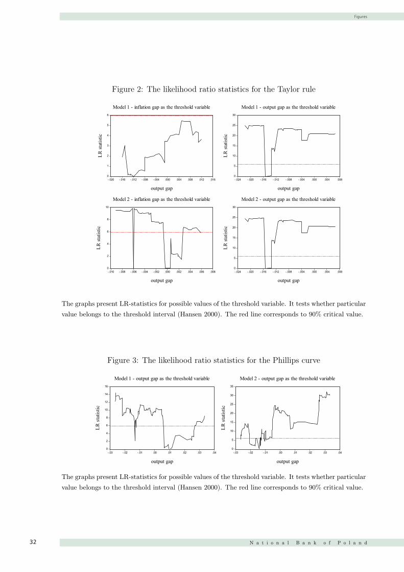
Figures
N a t i o n a l B a n k o f P o l a n d32
Figure 2: The likelihood ratio statistics for the Taylor rule
0
1
2
3
4
5
6
-.020 -.016 -.012 -.008 -.004 .000 .004 .008 .012 .016
output gap
LR st
atist
icModel 1 - inflation gap as the threshold variable
0
5
10
15
20
25
30
-.024 -.020 -.016 -.012 -.008 -.004 .000 .004 .008
output gap
LR st
atist
ic
Model 1 - output gap as the threshold variable
0
2
4
6
8
10
-.010 -.008 -.006 -.004 -.002 .000 .002 .004 .006 .008
output gap
LR st
atist
ic
Model 2 - inflation gap as the threshold variable
0
5
10
15
20
25
30
-.024 -.020 -.016 -.012 -.008 -.004 .000 .004 .008
output gap
LR st
atist
ic
Model 2 - output gap as the threshold variable
The graphs present LR-statistics for possible values of the threshold variable. It tests whether particularvalue belongs to the threshold interval (Hansen 2000). The red line corresponds to 90% critical value.
Figure 3: The likelihood ratio statistics for the Phillips curve
0
2
4
6
8
10
12
14
16
-.03 -.02 -.01 .00 .01 .02 .03 .04
output gap
LR s
tatis
tic
Model 1 - output gap as the threshold variable
0
5
10
15
20
25
30
35
-.03 -.02 -.01 .00 .01 .02 .03 .04
output gap
LR s
tatis
tic
Model 2 - output gap as the threshold variable
The graphs present LR-statistics for possible values of the threshold variable. It tests whether particularvalue belongs to the threshold interval (Hansen 2000). The red line corresponds to 90% critical value.
33