mortality and morbidity among t1d dn patientsbendixcarstensen.com/sdc/nefro/dn1.pdfchapter 1...
TRANSCRIPT

Mortality and morbidityamong T1D DN patients
GbAd, PRo / SDChttp://bendixcarstensen.com/SDC/Nefro/
December 2013Version 5.2
Compiled Wednesday 1st January, 2014, 22:01from: c:/Bendix/Steno/GbAd/DN1.tex
Bendix Carstensen Steno Diabetes Center, Gentofte, Denmark& Department of Biostatistics, University of Copenhagen
http://BendixCarstensen.com

Contents
1 Analysis of T1 patients’ follow-up 11.1 Analysis of rates . . . . . . . . . . . . . . . . . . . . . . . . . . . . . . . . . 2
1.1.1 Simple proportional hazards model . . . . . . . . . . . . . . . . . . . 71.1.2 CVD effect . . . . . . . . . . . . . . . . . . . . . . . . . . . . . . . . 91.1.3 Covariate effects . . . . . . . . . . . . . . . . . . . . . . . . . . . . . 101.1.4 Baseline effects . . . . . . . . . . . . . . . . . . . . . . . . . . . . . . 171.1.5 Time trends . . . . . . . . . . . . . . . . . . . . . . . . . . . . . . . . 22
1.2 Prediction of life course . . . . . . . . . . . . . . . . . . . . . . . . . . . . . . 22
ii

Chapter 1
Analysis of T1 patients’ follow-up
> library( Epi )> library( splines )
Initially we load the T1D patients from the datasets with the follow-up:
> load( file="./data/Base-Lexis.Rda" )> L1 <- subset( L1, dm.type=="type1" )> L7 <- subset( L7, dm.type=="type1" )
We can make a Lexis diagram of the follow-up with DN duration and age as timescales:
> ypi <- 7> yl <- c(15,90)> xl <- c(0,40)> pdf( "./graph/DN1-tfn-Lexis.pdf",+ height=1+diff(yl)/ypi,+ width=1+diff(xl)/ypi )> par( mai=c(3,3,1,1)/4, omi=c(0,0,0,0),+ mgp=c(3,1,0)/1.6, las=1 )> plsymb <- c(NA,16)[1+(substr(L7$lex.Xst,1,4)=="Dead")]> plot( L7,+ time.scale=c("tfn","age"), xlab="DN duration", ylab="Age",+ col=clr[L7$lex.Cst],+ xaxs="i", yaxs="i", xaxt="n", yaxt="n", xlim=xl, ylim=yl,+ grid=seq(10,90,5), lty.grid=1 )> axis( side=1, at=0:5*5, labels=rep("",6) )> axis( side=1, at=0:5*10 )> axis( side=2, at=0:20*5, labels=rep("",21) )> axis( side=2, at=0:20*10 )> points( L7, pch=plsymb, cex=0.7, col=clr[L7$lex.Cst] )> dev.off()
null device1
> xl <- c(0,15)+1998> pdf( "./graph/DN1-per-Lexis.pdf",+ height=1+diff(yl)/ypi,+ width=1+diff(xl)/ypi )> par( mai=c(3,3,1,1)/4, omi=c(0,0,0,0),+ mgp=c(3,1,0)/1.6, las=1 )> plsymb <- c(NA,16)[1+(substr(L7$lex.Xst,1,4)=="Dead")]> plot( L7,+ time.scale=c("per","age"), xlab="Date of FU", ylab="Age",+ col=clr[L7$lex.Cst],+ xaxs="i", yaxs="i", xaxt="n", yaxt="n", xlim=xl, ylim=yl,+ grid=seq(10,90,5), lty.grid=1 )> axis( side=1, at=0:5*5+2000, labels=rep("",6) )
1

2 Analysis of T1 patients’ follow-up T1D DN mortality
> axis( side=1, at=0:5*10+2000 )> axis( side=2, at=0:20*5, labels=rep("",21) )> axis( side=2, at=0:20*10 )> points( L7, pch=plsymb, cex=0.7, col=clr[L7$lex.Cst] )> dev.off()
null device1
> xl <- c(0,30)> X7 <- subset( L7, !is.na(tfCVD) )> pdf( "./graph/DN1-cvd-Lexis.pdf",+ height=1+diff(yl)/ypi,+ width=1+diff(xl)/ypi )> par( mai=c(3,3,1,1)/4, omi=c(0,0,0,0),+ mgp=c(3,1,0)/1.6, las=1 )> plsymb <- c(NA,16)[1+(substr(X7$lex.Xst,1,4)=="Dead")]> plot( X7,+ time.scale=c("tfCVD","age"), xlab="CVD duration", ylab="Age",+ col=clr[X7$lex.Cst],+ xaxs="i", yaxs="i", xaxt="n", yaxt="n", xlim=xl, ylim=yl,+ grid=seq(10,90,5), lty.grid=1 )> axis( side=1, at=0:5*5, labels=rep("",6) )> axis( side=1, at=0:5*10 )> axis( side=2, at=0:20*5, labels=rep("",21) )> axis( side=2, at=0:20*10 )> points( X7, pch=plsymb, cex=0.7, col=clr[X7$lex.Cst] )> dev.off()
null device1
We also make a plot of the actual transitions between states for T1D patients:
> bp <- list( x = c( 10, 40, 43, 19, 90, 90, 90, 90 ),+ y = c( 95, 65, 35, 5, 95, 65, 35, 5 ) )> boxes( L7, boxpos=bp, cex=1.2, lwd=3, wmult=1.1, hmult=1.3,+ show.BE="nz", BE.pre=c(""," ",""),+ scale.R=100, digits.R=1, DR.sep=c(" (",")"),+ col.bg=clx, col.txt=rep(c("white","black"),each=4),+ col.border=c(clx[1:4],rep("black",4)),+ col.arr=c(par("fg"),clr[c(2,1,4)])[c(1:3,2,3,4,1,4)],+ pos.arr=c(0.4,0.6)[c(1,2,1,1,1,1,2,1)] )
1.1 Analysis of rates
In order to analyze the transition rates we split the follow-up in small pieces of 2 monthduration along the timescale time since DN, called tfn:
> S7 <- splitLexis( L7, breaks=seq(0,100,1/6), time.scale="tfn" )> summary( S7 )
Transitions:To
From DN CVD ESRD+CVD ESRD Dead(DN) Dead(CVD) Dead(ESRD+CVD)DN 14949 70 0 92 34 0 0CVD 0 4976 56 0 0 42 0ESRD+CVD 0 0 1458 0 0 0 45ESRD 0 0 35 1544 0 0 0Sum 14949 5046 1549 1636 34 42 45
Transitions:To
From Dead(ESRD) Records: Events: Risk time: Persons:

Analysis of T1 patients’ follow-up 1.1 Analysis of rates 3
DN duration
Age
0 10 20 30 40
20
30
40
50
60
70
80
90
●
●
●
●
●
●
●
●
●
●
●
●
●
●
●
●
●
●
●
●
●
●
●
●
●
●
●
●
●
●
●
●
●
●
●
●
●
●
●
●
●
●
●●
●
●
●
●
●
●
●
●
●
●
●
●
●
●
●
●
●●
●
●
●
●
●
●
●
●
●
●
●
●
●
●
●
●
●
●
●
●
●
●
●
●
●
●
●
●
●
●
●
●
●
●
●
●
●
●
●
●
●
●
●
●
●
●
●
●
●
●
●
●
●
●
●
●
●
●
●
●
●
●
●
●
●
●
●
●
●
●
●
●
●
CVD duration
Age
0 10 20 30
20
30
40
50
60
70
80
90
●
●
●
●
●
●
●
●
●
●
●
●
●
●
●
●
●
●
●
●
●
●
●
●
●
●
●
●
●
●
●
●●
●
●
●
●
●
●
●
●
●
●
●
●
●
●
●
●
●
●
●
●
●
●
●
●
●
●
●
●
●
●
●
●
●
●
●
●
●
Date of FU
Age
2000 2010
20
30
40
50
60
70
80
90
●
●
●
●
●
●
●
●
●
●
●
●
●
●
●
●
●
●
●
●
●
●
●
●
●
●
●
●
●
●
●
●
●
●
●
●
●
●
●
●
●
●
● ●
●
●
●
●
●
●
●
●
●
●
●
●
●
●
●
●
●●
●
●
●
●
●
●
●
●
●
●
●
●
●
●
●
●
●
●
●
●
●
●
●
●
●
●
●
●
●
●
●
●
●
●
●
●
●
●
●
●
●
●
●
●
●
●
●
●
●
●
●
●
●
●
●
●
●
●
●
●
●
●
●
●
●
●
●
●
●
●
●
●
●
Figure 1.1: Lexis diagrams for the follow-up of T1 patients by DN duration, CVD durationand calendar time versus age. DN state is green, CVD blue, ESRD after CVD orange andESRD without CVD red. Dots indicate deaths.

4 Analysis of T1 patients’ follow-up T1D DN mortality
DN2,493.9
393 197
CVD824.7
104 76
ESRD+CVD235.5
46
ESRD250.0
43
Dead(DN) 34
Dead(CVD) 42
Dead(ESRD+CVD) 45
Dead(ESRD) 14
70 (2.8)
92 (3.7)
34 (1.4)
56 (6.8)
42 (5.1)
45 (19.1)
35 (14.0)
14 (5.6)
DN2,493.9
393 197
CVD824.7
104 76
ESRD+CVD235.5
46
ESRD250.0
43
Dead(DN) 34
Dead(CVD) 42
Dead(ESRD+CVD) 45
Dead(ESRD) 14
DN2,493.9
393 197
CVD824.7
104 76
ESRD+CVD235.5
46
ESRD250.0
43
Dead(DN) 34
Dead(CVD) 42
Dead(ESRD+CVD) 45
Dead(ESRD) 14
Figure 1.2: States and transitions between them in the analysis set-up for T1D patients.Numbers in the boxes are the person-years, and the number of persons starting, respectivelyending in each state. The numbers on the arrows are the number of transitions (rate per 100PY).Note that some persons start their follow-up in the CVD state; these patients also suffer fromDN.

Analysis of T1 patients’ follow-up 1.1 Analysis of rates 5
DN 0 15145 196 2493.86 393CVD 0 5074 98 824.70 174ESRD+CVD 0 1503 45 235.53 91ESRD 14 1593 49 249.96 92Sum 14 23315 388 3804.05 497
> addmargins(with(L7,table(table(lex.id))))
1 2 3 Sum302 137 58 497
> addmargins(with(S7,table(table(lex.id))))
1 2 3 4 6 7 8 9 10 11 12 14 15 16 17 18 19 20 21 223 2 1 3 5 4 3 9 4 6 2 4 5 3 4 2 6 6 4 423 24 25 26 27 28 29 30 31 32 33 34 35 36 37 38 39 40 41 421 7 2 6 7 5 6 2 10 2 4 6 14 10 5 4 2 4 3 943 44 45 46 47 48 49 50 51 52 53 54 55 56 57 58 59 60 61 625 4 2 5 8 2 5 3 2 5 5 7 2 5 9 7 14 11 16 2163 64 65 66 67 68 Sum25 41 30 50 22 2 497
We want to position the knots for the splines so that the number of events is the samebetween each pair of knots. We do this the same way for all transitions after inspection:
> nk <- 4> ( n.kn <- with( subset( S7, substr(lex.Xst,1,4)=="Dead" ),+ quantile( tfn+lex.dur, probs=(1:nk-0.5)/nk ) ) )
12.5% 37.5% 62.5% 87.5%6.512834 11.613963 15.953799 22.643395
> ( a.kn <- with( subset( S7, substr(lex.Xst,1,4)=="Dead" ),+ quantile( age+lex.dur, probs=(1:nk-0.5)/nk ) ) )
12.5% 37.5% 62.5% 87.5%43.39493 53.93977 63.35524 74.02259
> ( d.kn <- with( subset( S7, substr(lex.Xst,1,4)=="Dead" ),+ quantile( dur+lex.dur, probs=(1:nk-0.5)/nk ) ) )
12.5% 37.5% 62.5% 87.5%21.22519 31.26626 39.30459 49.35164
Since we are interested in modelling the transitions in figure 1.2, we make a stacked datasetand use this as the basis for modelling:
> St7 <- stack( S7 )> dim( St7 )
[1] 60272 40
> xtabs( cbind(lex.dur,lex.Fail) ~ lex.Tr, data=St7 )
lex.Tr lex.dur lex.FailDN->CVD 2493.8563 70.0000DN->ESRD 2493.8563 92.0000DN->Dead(DN) 2493.8563 34.0000CVD->ESRD+CVD 824.7036 56.0000CVD->Dead(CVD) 824.7036 42.0000ESRD+CVD->Dead(ESRD+CVD) 235.5291 45.0000ESRD->ESRD+CVD 249.9576 35.0000ESRD->Dead(ESRD) 249.9576 14.0000
We are not (initially) interested in the first and last three of these transitions, so we subsetto the relevant 4 transitions; we specifically want to look at mortality rates and rates ofESRD from the states DN and CVD. We just check that all is as expected:

6 Analysis of T1 patients’ follow-up T1D DN mortality
> St4 <- subset( St7, lex.Tr %in% levels(St7$lex.Tr)[2:5] )> St4$lex.Tr <- factor( St4$lex.Tr )> with( St4, ftable( lex.Xst, lex.Tr, lex.Fail,col.vars=2:3 ) )
lex.Tr DN->ESRD DN->Dead(DN) CVD->ESRD+CVD CVD->Dead(CVD)lex.Fail FALSE TRUE FALSE TRUE FALSE TRUE FALSE TRUE
lex.XstDN 14949 0 14949 0 0 0 0 0CVD 70 0 70 0 4976 0 4976 0ESRD+CVD 0 0 0 0 0 56 56 0ESRD 0 92 92 0 0 0 0 0Dead(DN) 34 0 0 34 0 0 0 0Dead(CVD) 0 0 0 0 42 0 0 42Dead(ESRD+CVD) 0 0 0 0 0 0 0 0Dead(ESRD) 0 0 0 0 0 0 0 0
> dim( St4 )
[1] 40438 40

Analysis of T1 patients’ follow-up 1.1 Analysis of rates 7
1.1.1 Simple proportional hazards model
We now set up a simple model that just models the 4 different transitions using the samedependency on time since DN, diabetes duration, sex and current age. Note that this modelassumes that all 4 types of rates are proportional along the three chosen timescales:
> m0 <- glm( lex.Fail ~ lex.Tr + sex ++ Ns( tfn, kn=n.kn ) ++ Ns( age, kn=a.kn ) ++ Ns( dur, kn=d.kn ),+ offset=log(lex.dur), family=poisson,+ data = St4 )> round( ci.exp( m0 ), 3 )
exp(Est.) 2.5% 97.5%(Intercept) 0.028 0.019 0.041lex.TrDN->Dead(DN) 0.370 0.249 0.548lex.TrCVD->ESRD+CVD 1.627 1.155 2.291lex.TrCVD->Dead(CVD) 1.220 0.839 1.774sexM 1.258 0.943 1.679Ns(tfn, kn = n.kn)1 0.922 0.563 1.509Ns(tfn, kn = n.kn)2 1.361 0.816 2.271Ns(tfn, kn = n.kn)3 1.110 0.741 1.663Ns(age, kn = a.kn)1 1.791 1.070 2.999Ns(age, kn = a.kn)2 2.689 1.694 4.270Ns(age, kn = a.kn)3 2.742 1.759 4.275Ns(dur, kn = d.kn)1 0.592 0.352 0.996Ns(dur, kn = d.kn)2 0.685 0.399 1.175Ns(dur, kn = d.kn)3 0.615 0.393 0.962
> CM <- rbind(0,c(1,0,0),c(0,1,0),c(0,-1,1),c(-1,0,1))> rownames( CM ) <- paste( c("",levels(St4$lex.Tr)[c(2:4,4)]),+ c("",rep(" vs. ",4)),+ levels(St4$lex.Tr)[c(1,1,1,3,2)], sep="" )> colnames( CM ) <- levels(St4$lex.Tr)[-1]> CM
DN->Dead(DN) CVD->ESRD+CVD CVD->Dead(CVD)DN->ESRD 0 0 0DN->Dead(DN) vs. DN->ESRD 1 0 0CVD->ESRD+CVD vs. DN->ESRD 0 1 0CVD->Dead(CVD) vs. CVD->ESRD+CVD 0 -1 1CVD->Dead(CVD) vs. DN->Dead(DN) -1 0 1
> round( ci.exp( m0, subset="lex.Tr" ), 2 )
exp(Est.) 2.5% 97.5%lex.TrDN->Dead(DN) 0.37 0.25 0.55lex.TrCVD->ESRD+CVD 1.63 1.15 2.29lex.TrCVD->Dead(CVD) 1.22 0.84 1.77
> round( ci.exp( m0, subset="lex.Tr", ctr.mat=CM ), 2 )
exp(Est.) 2.5% 97.5%DN->ESRD 1.00 1.00 1.00DN->Dead(DN) vs. DN->ESRD 0.37 0.25 0.55CVD->ESRD+CVD vs. DN->ESRD 1.63 1.15 2.29CVD->Dead(CVD) vs. CVD->ESRD+CVD 0.75 0.50 1.12CVD->Dead(CVD) vs. DN->Dead(DN) 3.30 2.08 5.23
This means that CVD influences the occurrence of ESRD by a factor of 1.6, whereas thereis a 3.3-fold increase in the rate of death (prior to ESRD).
We can then test the proportionality of the rates on each of the three timescales:
> ma <- update( m0 , .~. + lex.Tr:Ns(age,kn=a.kn) )> mna <- update( ma , .~. + lex.Tr:Ns(tfn,kn=n.kn) )> mnad <- update( mna , .~. + lex.Tr:Ns(dur,kn=d.kn) )> mad <- update( mnad, .~. - lex.Tr:Ns(tfn,kn=n.kn) )> pr.test <- anova( m0, ma, mna, mnad, mad, ma, test="Chisq" )[-1,3:5]> rownames( pr.test ) <- c("+i.age","+i.tfn","+i.dur","-i.tfn","-i.dur")> round( pr.test, 3 )

8 Analysis of T1 patients’ follow-up T1D DN mortality
Df Deviance Pr(>Chi)+i.age 9 19.592 0.021+i.tfn 9 12.453 0.189+i.dur 9 7.146 0.622-i.tfn -9 -11.786 0.226-i.dur -9 -7.813 0.553
If anything, the rates are non-proportional along the age-scale, but hardly along any of theother time scales. However, these tests are somewhat unspecific as they test forproportionality of 4 different transitions simultaneously; it is of more interest to see if thereis proportionality between pairs of these. More precisely, it is more relevant to test thestate×timescale interaction for one set of transitions at at time. Specifically we want totest proportionality between pairs of rates:
1. Death and ESRD rates from the DN state (fromDN)
2. Death and ESRD rates from the CVD state (fromCVD)
3. Death rates from the DN and CVD states (toDeath)
4. ESRD rates from the DN and CVD states (toESRD)
However we would also like to see if these non-proportionalities are confounded by theclinical variables of interest.
Each of these sets of proportionality assumptions are testable by fitting the same set ofmodels as above, but varying the outcome and the dataset:
> log1.5 <- function(x) log(x)/log(1.5)> mz <- update( m0, . ~ . + bmi+ + I(sys.bt/10)+ + I(-gfr/10)+ + log2(alb)+ + log1.5(pmax(ins.kg,0.03))+ + hmgb+ + hba1c+ + tchol+ + bmi+ + smoke )> mx <- update( mz, data=subset(St4,lex.Tr %in% c("DN->Dead(DN)","DN->ESRD") ) )> ma <- update( mx , .~. + lex.Tr:Ns(age,kn=a.kn) )> mna <- update( ma , .~. + lex.Tr:Ns(tfn,kn=n.kn) )> mnad <- update( mna , .~. + lex.Tr:Ns(dur,kn=d.kn) )> mad <- update( mnad, .~. - lex.Tr:Ns(tfn,kn=n.kn) )> pr.fromDN <- anova( mx, ma, mna, mnad, mad, ma, test="Chisq" )[-1,3:5]> rownames( pr.fromDN ) <- c("+i.age","+i.tfn","+i.dur","-i.tfn","-i.dur")> mx <- update( mz, data=subset(St4,lex.Tr %in% c("CVD->Dead(CVD)","CVD->ESRD+CVD") ) )> ma <- update( mx , .~. + lex.Tr:Ns(age,kn=a.kn) )> mna <- update( ma , .~. + lex.Tr:Ns(tfn,kn=n.kn) )> mnad <- update( mna , .~. + lex.Tr:Ns(dur,kn=d.kn) )> mad <- update( mnad, .~. - lex.Tr:Ns(tfn,kn=n.kn) )> pr.fromCVD <- anova( mx, ma, mna, mnad, mad, ma, test="Chisq" )[-1,3:5]> rownames( pr.fromCVD ) <- c("+i.age","+i.tfn","+i.dur","-i.tfn","-i.dur")> mx <- update( mz, data=subset(St4,lex.Tr %in% c("DN->Dead(DN)","CVD->Dead(CVD)") ) )> ma <- update( mx , .~. + lex.Tr:Ns(age,kn=a.kn) )> mna <- update( ma , .~. + lex.Tr:Ns(tfn,kn=n.kn) )> mnad <- update( mna , .~. + lex.Tr:Ns(dur,kn=d.kn) )> mad <- update( mnad, .~. - lex.Tr:Ns(tfn,kn=n.kn) )> pr.toDeath <- anova( mx, ma, mna, mnad, mad, ma, test="Chisq" )[-1,3:5]> rownames( pr.toDeath ) <- c("+i.age","+i.tfn","+i.dur","-i.tfn","-i.dur")> mx <- update( mz , data=subset(St4,lex.Tr %in% c("DN->ESRD","CVD->ESRD+CVD") ) )> ma <- update( mx , .~. + lex.Tr:Ns(age,kn=a.kn) )
Analysis of T1 patients’ follow-up 1.1 Analysis of rates 9
> mna <- update( ma , .~. + lex.Tr:Ns(tfn,kn=n.kn) )> mnad <- update( mna , .~. + lex.Tr:Ns(dur,kn=d.kn) )> mad <- update( mnad, .~. - lex.Tr:Ns(tfn,kn=n.kn) )> pr.toESRD <- anova( mx, ma, mna, mnad, mad, ma, test="Chisq" )[-1,3:5]> rownames( pr.toESRD ) <- c("+i.age","+i.tfn","+i.dur","-i.tfn","-i.dur")> prop <- cbind( pr.fromDN, pr.fromCVD, pr.toDeath, pr.toESRD )> colnames( prop )[0:3*3+1] <- c("fromDN","fromCVD","toDeath","toESRD")> round( prop[,1:6], 3 )
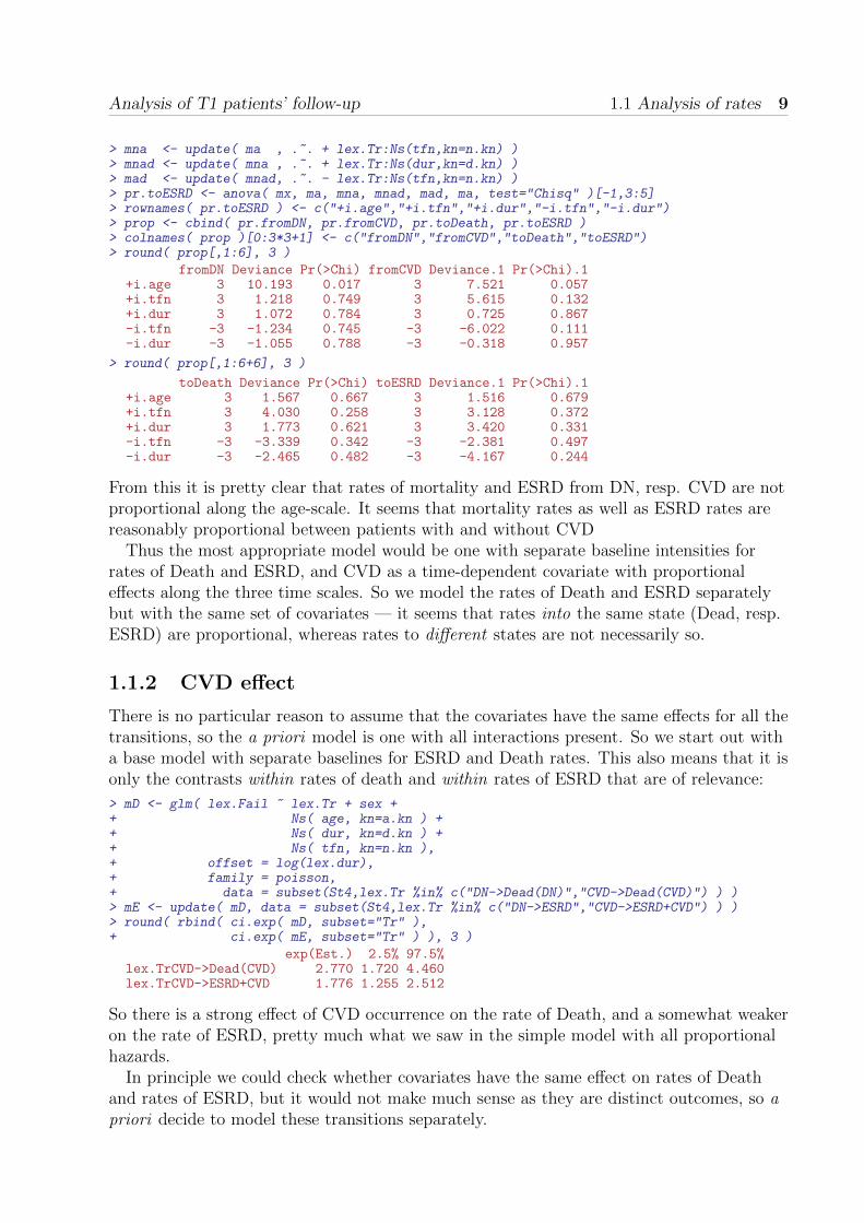
fromDN Deviance Pr(>Chi) fromCVD Deviance.1 Pr(>Chi).1+i.age 3 10.193 0.017 3 7.521 0.057+i.tfn 3 1.218 0.749 3 5.615 0.132+i.dur 3 1.072 0.784 3 0.725 0.867-i.tfn -3 -1.234 0.745 -3 -6.022 0.111-i.dur -3 -1.055 0.788 -3 -0.318 0.957
> round( prop[,1:6+6], 3 )
toDeath Deviance Pr(>Chi) toESRD Deviance.1 Pr(>Chi).1+i.age 3 1.567 0.667 3 1.516 0.679+i.tfn 3 4.030 0.258 3 3.128 0.372+i.dur 3 1.773 0.621 3 3.420 0.331-i.tfn -3 -3.339 0.342 -3 -2.381 0.497-i.dur -3 -2.465 0.482 -3 -4.167 0.244
From this it is pretty clear that rates of mortality and ESRD from DN, resp. CVD are notproportional along the age-scale. It seems that mortality rates as well as ESRD rates arereasonably proportional between patients with and without CVD
Thus the most appropriate model would be one with separate baseline intensities forrates of Death and ESRD, and CVD as a time-dependent covariate with proportionaleffects along the three time scales. So we model the rates of Death and ESRD separatelybut with the same set of covariates — it seems that rates into the same state (Dead, resp.ESRD) are proportional, whereas rates to different states are not necessarily so.
1.1.2 CVD effect
There is no particular reason to assume that the covariates have the same effects for all thetransitions, so the a priori model is one with all interactions present. So we start out witha base model with separate baselines for ESRD and Death rates. This also means that it isonly the contrasts within rates of death and within rates of ESRD that are of relevance:
> mD <- glm( lex.Fail ~ lex.Tr + sex ++ Ns( age, kn=a.kn ) ++ Ns( dur, kn=d.kn ) ++ Ns( tfn, kn=n.kn ),+ offset = log(lex.dur),+ family = poisson,+ data = subset(St4,lex.Tr %in% c("DN->Dead(DN)","CVD->Dead(CVD)") ) )> mE <- update( mD, data = subset(St4,lex.Tr %in% c("DN->ESRD","CVD->ESRD+CVD") ) )> round( rbind( ci.exp( mD, subset="Tr" ),+ ci.exp( mE, subset="Tr" ) ), 3 )
exp(Est.) 2.5% 97.5%lex.TrCVD->Dead(CVD) 2.770 1.720 4.460lex.TrCVD->ESRD+CVD 1.776 1.255 2.512
So there is a strong effect of CVD occurrence on the rate of Death, and a somewhat weakeron the rate of ESRD, pretty much what we saw in the simple model with all proportionalhazards.
In principle we could check whether covariates have the same effect on rates of Deathand rates of ESRD, but it would not make much sense as they are distinct outcomes, so apriori decide to model these transitions separately.

10 Analysis of T1 patients’ follow-up T1D DN mortality
1.1.3 Covariate effects
Hence we make separate models for the two transitions based on subsets of the splitdataset, S7. But we will only use the part of the dataset that relates to the transitions weare looking at, so the part where lex.Cst %in% %c("DN","CVD"):
> S7d <- Relevel( subset( S7, lex.Cst %in% c("DN","CVD") ),+ list("Dead"=5:8), first=FALSE )
type old new1 lex.Cst DN DN2 lex.Cst CVD CVD3 lex.Cst ESRD+CVD4 lex.Cst ESRD5 lex.Cst Dead(DN)6 lex.Cst Dead(CVD)7 lex.Cst Dead(ESRD+CVD)8 lex.Cst Dead(ESRD)9 lex.Xst DN DN10 lex.Xst CVD CVD11 lex.Xst ESRD+CVD ESRD+CVD12 lex.Xst ESRD ESRD13 lex.Xst Dead(DN) Dead14 lex.Xst Dead(CVD) Dead15 lex.Xst Dead(ESRD+CVD)16 lex.Xst Dead(ESRD)
> summary( S7d )
Transitions:To
From DN CVD ESRD+CVD ESRD Dead Records: Events: Risk time: Persons:DN 14949 70 0 92 34 15145 196 2493.86 393CVD 0 4976 56 0 42 5074 98 824.70 174Sum 14949 5046 56 92 76 20219 294 3318.56 497
We shall also address the mortality subsequent to ESRD, so we make a dataset for theanalysis of these transitions too:
> S7e <- Relevel( subset( S7, lex.Cst %in% c("ESRD","ESRD+CVD") ),+ list("Dead"=5:8), first=FALSE )
type old new1 lex.Cst DN2 lex.Cst CVD3 lex.Cst ESRD+CVD ESRD+CVD4 lex.Cst ESRD ESRD5 lex.Cst Dead(DN)6 lex.Cst Dead(CVD)7 lex.Cst Dead(ESRD+CVD)8 lex.Cst Dead(ESRD)9 lex.Xst DN10 lex.Xst CVD11 lex.Xst ESRD+CVD ESRD+CVD12 lex.Xst ESRD ESRD13 lex.Xst Dead(DN)14 lex.Xst Dead(CVD)15 lex.Xst Dead(ESRD+CVD) Dead16 lex.Xst Dead(ESRD) Dead
> summary( S7e )
Transitions:To
From DN CVD ESRD+CVD ESRD Dead Records: Events: Risk time: Persons:ESRD+CVD 0 0 1458 0 45 1503 45 235.53 91ESRD 0 0 35 1544 14 1593 49 249.96 92Sum 0 0 1493 1544 59 3096 94 485.49 148

Analysis of T1 patients’ follow-up 1.1 Analysis of rates 11
The naming convention is having the first uppercase letter as B for models withoutcovariates or E for models extended with covariates, followed by a lowercase d for deathswithout ESRD, e for ESRD events and ed for deaths subsequent to ESRD:
> # Base model:> Bd <- glm( lex.Xst=="Dead" ~ Ns( age, kn=a.kn ) ++ Ns( dur, kn=d.kn ) ++ Ns( tfn, kn=n.kn ) ++ I(lex.Cst=="CVD") + sex,+ offset = log(lex.dur),+ family = poisson,+ data = S7d )> # Extend model by adding covariates:> Ed <- update( Bd, . ~ . + bmi ++ + I(sys.bt/10)+ + I(-gfr/10)+ + log2(alb)+ + log1.5(pmax(ins.kg,0.03))+ + hmgb+ + hba1c+ + tchol+ + bmi+ + smoke )> # Model for ESRD coccurrence> Be <- update( Bd, substr(lex.Xst,1,4)=="ESRD" ~ . )> Ee <- update( Ed, substr(lex.Xst,1,4)=="ESRD" ~ . )> # Model for post-ESRD mortality> Bed <- update( Bd, . ~ . - I(lex.Cst=="CVD") + I(lex.Cst=="ESRD+CVD"), data=S7e )> Eed <- update( Ed, . ~ . - I(lex.Cst=="CVD") + I(lex.Cst=="ESRD+CVD"), data=S7e )
When looking at the results of the CVD-effects we should keep in mind that for most CVDpatients the baseline values are measured after the CVD date as illustrated in figure 1.3.
> par( mar=c(3,3,1,1), mgp=c(3,1,0)/1.6 )> with( L1,+ hist( docvd-donra,+ breaks=seq(-26,11,1), col="gray", main="",+ xlab="Time from entry to CVD (years)",+ ylim=c(0,20),xlim=c(-26,13) ) )> abline( v=0, col="red" )> text(-15, 12, paste("\nCVD: ",+ sum(!is.na(L1$docvd) ),+ "\nno CVD: ",+ sum( is.na(L1$docvd) ),+ sep=""),+ adj=c(1,1) )
The effects on the rates of death are now extracted; the first line is the isolated effect ofCVD, only taking duration of DN, duration of diabetes and age (=duration of life) intoaccount, the second line is the CVD effect controlled for all the other covariates. Thesubsequent lines are the effects of the covariates.
> dd <- rbind( ci.exp(Bd,subset="CVD"),+ ci.exp(Ed,subset=-(1:10)) )> round( dd, 3 )
exp(Est.) 2.5% 97.5%I(lex.Cst == "CVD")TRUE 2.770 1.720 4.460I(lex.Cst == "CVD")TRUE 2.578 1.554 4.277sexM 1.078 0.604 1.925bmi 0.942 0.863 1.028I(sys.bt/10) 1.029 0.886 1.195I(-gfr/10) 1.180 1.060 1.314log2(alb) 0.974 0.851 1.115

12 Analysis of T1 patients’ follow-up T1D DN mortality
Time from entry to CVD (years)
Fre
quen
cy
−20 −10 0 10
05
1015
20
CVD: 209no CVD: 288
Figure 1.3: Histogram of time from entry (date of DN) to CVD; hence, negative numbersrefer to patients with CVD prior to entry. Note that the numbers w/o CVD here is the totalnumber in the database, also those 34 who have a recorded date of CVD after ESRD, andwho thus do not appear in figure 1.2.
Analysis of T1 patients’ follow-up 1.1 Analysis of rates 13
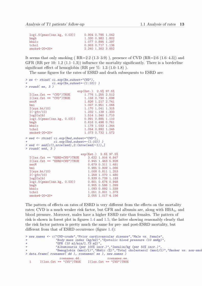
log1.5(pmax(ins.kg, 0.03)) 0.904 0.785 1.042hmgb 1.330 0.982 1.802hba1c 1.077 0.895 1.297tchol 0.903 0.717 1.136smoke4-20+20+ 2.240 1.302 3.852
It seems that only smoking ( RR=2.2 (1.3–3.9) ), presence of CVD (RR=2.6 (1.6–4.3)) andGFR (RR per 10: 1.2 (1.1–1.3)) influence the mortality significantly. There is a borderlinesignificant effect of hemoglobin (RR per %: 1.3 (1.0–1.8) ).
The same figures for the rates of ESRD and death subsequents to ESRD are:
> ee <- rbind( ci.exp(Be,subset="CVD"),+ ci.exp(Ee,subset=-(1:10)) )> round( ee, 3 )
exp(Est.) 2.5% 97.5%I(lex.Cst == "CVD")TRUE 1.776 1.255 2.512I(lex.Cst == "CVD")TRUE 1.158 0.790 1.698sexM 1.826 1.217 2.741bmi 1.007 0.951 1.066I(sys.bt/10) 1.170 1.041 1.315I(-gfr/10) 1.232 1.138 1.333log2(alb) 1.514 1.340 1.710log1.5(pmax(ins.kg, 0.03)) 0.991 0.885 1.110hmgb 0.616 0.498 0.761hba1c 1.178 1.033 1.344tchol 1.054 0.892 1.245smoke4-20+20+ 1.073 0.732 1.572
> eed <- rbind( ci.exp(Bed,subset="CVD"),+ ci.exp(Eed,subset=-(1:10)) )> eed <- eed[c(1,nrow(eed),2:(nrow(eed)-1)),]> round( eed, 3 )
exp(Est.) 2.5% 97.5%I(lex.Cst == "ESRD+CVD")TRUE 3.622 1.916 6.847I(lex.Cst == "ESRD+CVD")TRUE 2.945 1.463 5.928sexM 0.679 0.311 1.481bmi 0.985 0.909 1.066I(sys.bt/10) 1.008 0.811 1.253I(-gfr/10) 1.259 1.070 1.480log2(alb) 0.939 0.739 1.193log1.5(pmax(ins.kg, 0.03)) 0.801 0.676 0.948hmgb 0.905 0.586 1.399hba1c 1.093 0.892 1.339tchol 1.051 0.801 1.379smoke4-20+20+ 2.055 1.017 4.156
The pattern of effects on rates of ESRD is very different from the effects on the mortalityrates; CVD is a much weaker risk factor, but GFR and albumin are, along with HBA1c andblood pressure. Moreover, males have a higher ESRD rate than females. The pattern ofrisk is shown in forest plot in figures 1.4 and 1.5, the latter showing reasonably clearly thatthe risk factor pattern is pretty much the same for pre- and post-ESRD mortality, butdifferent from that of ESRD occurrence (figure 1.4):
> new.names <- c("CVD-crude","Prior cardiovascular disease","Male vs. female",+ "Body mass index (kg/m2)","Systolic blood pressure (10 mmHg)",+ "GFR (10 ml/min/1.73 m2)",+ "Albuminuria (per 100% incr.)","Insulin/kg (per 50% incr.)",+ "Hemoglobin (mmol/l)","HbA1c (%)","Total cholesterol (mmol/l)","Smoker vs. non-smoker")> data.frame( rownames( dd ), rownames( ee ), new.names )
rownames.dd. rownames.ee.1 I(lex.Cst == "CVD")TRUE I(lex.Cst == "CVD")TRUE

14 Analysis of T1 patients’ follow-up T1D DN mortality
2 I(lex.Cst == "CVD")TRUE I(lex.Cst == "CVD")TRUE3 sexM sexM4 bmi bmi5 I(sys.bt/10) I(sys.bt/10)6 I(-gfr/10) I(-gfr/10)7 log2(alb) log2(alb)8 log1.5(pmax(ins.kg, 0.03)) log1.5(pmax(ins.kg, 0.03))9 hmgb hmgb10 hba1c hba1c11 tchol tchol12 smoke4-20+20+ smoke4-20+20+
new.names1 CVD-crude2 Prior cardiovascular disease3 Male vs. female4 Body mass index (kg/m2)5 Systolic blood pressure (10 mmHg)6 GFR (10 ml/min/1.73 m2)7 Albuminuria (per 100% incr.)8 Insulin/kg (per 50% incr.)9 Hemoglobin (mmol/l)10 HbA1c (%)11 Total cholesterol (mmol/l)12 Smoker vs. non-smoker
> data.frame( rownames( dd ), rownames( eed ), new.names )
rownames.dd. rownames.eed.1 I(lex.Cst == "CVD")TRUE I(lex.Cst == "ESRD+CVD")TRUE2 I(lex.Cst == "CVD")TRUE I(lex.Cst == "ESRD+CVD")TRUE3 sexM sexM4 bmi bmi5 I(sys.bt/10) I(sys.bt/10)6 I(-gfr/10) I(-gfr/10)7 log2(alb) log2(alb)8 log1.5(pmax(ins.kg, 0.03)) log1.5(pmax(ins.kg, 0.03))9 hmgb hmgb10 hba1c hba1c11 tchol tchol12 smoke4-20+20+ smoke4-20+20+
new.names1 CVD-crude2 Prior cardiovascular disease3 Male vs. female4 Body mass index (kg/m2)5 Systolic blood pressure (10 mmHg)6 GFR (10 ml/min/1.73 m2)7 Albuminuria (per 100% incr.)8 Insulin/kg (per 50% incr.)9 Hemoglobin (mmol/l)10 HbA1c (%)11 Total cholesterol (mmol/l)12 Smoker vs. non-smoker
> rownames( dd ) <- rownames( ee ) <- rownames( eed ) <- new.names> par( mar=c(3,3,1,1), mgp=c(3,1,0)/1.6 )> rownames( dd )[c(4,6,10)] <- ""> plotEst( dd[-1,1:3], xlog=TRUE, vref=1, y=c(11:1), txtpos=c(11:1),+ lwd=3, cex=1.1, xlab="",+ xtic=c(0.4,0.6,1,2,4), xlim=c(0.4,4*16^2),+ grid=c(4:15/10,seq(2,4,0.5)),+ restore.par=FALSE )> axis( side=2, at=c(9,7,3),+ labels=c( expression( "Body mass index (kg/"*m^2*")" ),+ expression( "GFR (-10 ml/min/1.73"*m^2*")" ),+ expression( HbA[1][c]*"(%)" ) ),+ las=1, tick=FALSE )> abline( v=c(4:15/10,seq(2,4,0.5))*16, col=gray(0.9) )

Analysis of T1 patients’ follow-up 1.1 Analysis of rates 15
> abline( v=16 )> axis( side=1, at=c(0.4,0.6,1,2,4)*16, labels=formatC(c(0.4,0.6,1,2,4),format="f",digits=1) )> et <- pmax( ee, 0.4 )*16> linesEst( et[-1,1:3], vref=1, y=11:1, lwd=3, cex=1.1)> abline( v=c(4:15/10,seq(2,4,0.5))*16^2, col=gray(0.9) )> abline( v=16^2 )> axis( side=1, at=c(0.4,0.6,1,2,4)*16^2, labels=formatC(c(0.4,0.6,1,2,4),format="f",digits=1) )> et <- pmax( eed, 0.4 )*(16^2)> linesEst( et[-1,1:3], vref=1, y=11:1, lwd=3, cex=1.1)> mtext( "RR of pre-ESRD death" , side=1, line=par("mgp")[1], at=sqrt(10)*0.4 )> mtext( "RR of ESRD" , side=1, line=par("mgp")[1], at=sqrt(10)*0.4*16 )> mtext( "RR of post-ESRD death", side=1, line=par("mgp")[1], at=sqrt(10)*0.4*16^2 )
We could also show the effects of the covariates on the same scale for comparability,using different colors:
> par( mar=c(5,3,1,1), mgp=c(3,1,0)/1.6 )> plotEst( dd[-1,1:3], xlog=TRUE, vref=1, y=c(11:1)+0.15, txtpos=c(11:1),+ lwd=3, cex=1.1, xlab="",+ xtic=c(0.4,0.6,1,2,4), xlim=c(0.4,4),+ grid=c(4:15/10,seq(2,4,0.5)), col=clr[1],+ restore.par=FALSE )> axis( side=2, at=c(9,7,3),+ labels=c( expression( "Body mass index (kg/"*m^2*")" ),+ expression( "GFR (-10 ml/min/1.73"*m^2*")" ),+ expression( HbA[1][c]*"(%)" ) ),+ las=1, tick=FALSE )> et <- pmax( ee, 0.4 )> linesEst( et[-1,1:3], y=11:1-0.15, lwd=3, cex=1.1, col=clr[2])> et <- pmax( eed, 0.4 )> linesEst( et[-1,1:3], y=11:1 , lwd=3, cex=1.1, col=clr[4])> mtext( "RR of pre-ESRD death" , side=1, line=par("mgp")[1] , at=sqrt(10)*0.4, col=clr[1])> mtext( "RR of ESRD" , side=1, line=par("mgp")[1]+2, at=sqrt(10)*0.4, col=clr[2])> mtext( "RR of post-ESRD death", side=1, line=par("mgp")[1]+1, at=sqrt(10)*0.4, col=clr[4])
From figures 1.4 and 1.5 it is clear that the major risk factors for death are CVD, GFRand smoking, whereas the significant risk factors for ESRD are blood pressure, GFR,
●
●
●
●
●
●
●
●
●
●
●
0.4 1.0 2.0 4.0
Smoker vs. non−smoker
Total cholesterol (mmol/l)
Hemoglobin (mmol/l)
Insulin/kg (per 50% incr.)
Albuminuria (per 100% incr.)
Systolic blood pressure (10 mmHg)
Male vs. female
Prior cardiovascular disease
HbA1c(%)
GFR (−10 ml/min/1.73m2)
Body mass index (kg/m2)
0.4 1.0 2.0 4.0
●
●
●
●
●
●
●
●
●
●
●
0.4 1.0 2.0 4.0
●
●
●
●
●
●
●
●
●
●
●
RR of pre−ESRD death RR of ESRD RR of post−ESRD death
Figure 1.4: RRs associated with the different risk factors for the transitions from DN andCVD, to either death or ESRD or from ESRD to death (see figure 1.2).

16 Analysis of T1 patients’ follow-up T1D DN mortality
●
●
●
●
●
●
●
●
●
●
●
0.4 0.6 1.0 2.0 4.0
Smoker vs. non−smoker
Total cholesterol (mmol/l)
Hemoglobin (mmol/l)
Insulin/kg (per 50% incr.)
Albuminuria (per 100% incr.)
Systolic blood pressure (10 mmHg)
Male vs. female
Prior cardiovascular disease
HbA1c(%)
GFR (−10 ml/min/1.73m2)
Body mass index (kg/m2)
●
●
●
●
●
●
●
●
●
●
●
●
●
●
●
●
●
●
●
●
●
●
RR of pre−ESRD death
RR of ESRDRR of post−ESRD death
Figure 1.5: RRs associated with the different risk factors for the transitions from DN andCVD, to either death or ESRD or from ESRD to death (see figure 1.2).

Analysis of T1 patients’ follow-up 1.1 Analysis of rates 17
albuminuria, HbA1c and low hemoglobin.
1.1.4 Baseline effects
These RR estimates are all conditional on the baseline hazard which depends on time sinceentry (tfn), duration of diabetes (dur) and current age (age).
> quantile( L1$lex.dur, probs=0:4/4 )
0% 25% 50% 75% 100%0.02737851 5.09787817 9.13347023 10.54893908 10.98973306
> pairs( L1[,c("age","tfn","dur")], gap=0, pch=16 )
We want to show the mortality rates as a function of time since DN for times from 0 to10 years. Since the mortality also depends on DM duration and current age, we need totake these into account too, so draw mortality curves for different combinations of age andduration at entry. Moreover, we will of course also need to fix the values of the othercovariates, so we just get an overview of the distribution of the covariates as measured atbaseline:
age
0 10 20 30 40
●
●
●
●
●
●
●
●
●
●
●
●
●
●●
● ●
●
●
●
●●
●
● ●
●
●
●
●
●●●
●●
●
●
●
●●
●
●●
●
●
●
●
●
●
●●
●
● ●●
●●
●
● ●
●
●
●
●
●
●
●
●
●●
●
●
●
●
●
●●
●
●
●
●●
●
●
●
●
●
●
●
●
●
●
●●
●
●●
●
●
●
●
●
●
●
●
●
●●
●
●●
●
●
●●
●
●
●
●●
●
●
●
●
●
●
●
●
●
●
●●
●●●
●
●
●
●
●
●
●
●
●
● ●
●
●
●
●
●
●
●
●
●
●
●
●
●●●
●●●
●
●●
●
●
●
●●●
●
●
●●
●
●
●
●●
●
●
●
●
●●
● ●
●
●
●●
● ●
●
●
●●●
●
●
●
●
●
●
●
● ●●
●
●
●
●
●
●
●
●●
●●
●
●
●
●
●●
●
●●
●
●●
●●
●
●
●
●
●
●
●
●
●●
●
●●●
●● ●
●
●
●
●
●
●●
●
●
●●
●
●
●●
●
●
●
●
●
●
●
●
●
●
●
●
●
●
●●
●
●
●
●
●
●
●
●
●
●
●
●
●●
●
●
●●●
●
●
●
●
●●●
●
●●
●
●
●●
●
●
●
●
●
●
●
●
●
●
●
●
●
●
● ●●
●
●
●
●
●●
●
●
●
●
●
●●
●
●●
●
●
●
●
●●
●
●
●
●
●
●
●
●
●
●
●●
●
●
●
●
●
●
●
●
●
●
●
●
●
●
●
●●
●
●
●
●
●●
●
●
●
●
●
●
●
●
●
●●
●●●
●
●
●
●
●
● ●●
●
●
●
●
●
●
●
●
● ●●
●
●●
●●
●
●
●
●
●
●
●
● ●
●●
●
●
●●
●
●
●●
●
●
●
●
●
●
●
●
●
● ●
●
●●
●●
●
●
●
●
●
●●
●
●
●
●
●
●
●
●
●
●
●
●
● ●●
●
●●
●
●
●
●
●
●
●
●
●20
3040
5060
7080
●
●
●
●
●
●
●
●
●
●
●
●
●
●●
● ●
●
●
●
●●
●
● ●
●
●
●
●
●●●
●●
●
●
●
●●
●
●●
●
●
●
●
●
●
●●
●
●●●
●●
●
●●
●
●
●
●
●
●
●
●
●●
●
●
●
●
●
● ●
●
●
●
●●
●
●
●
●
●
●
●
●
●
●
●●
●
●●
●
●
●
●
●
●
●
●
●
●●
●
●●
●
●
●●
●
●
●
●●
●
●
●
●
●
●
●
●
●
●
●●
●● ●
●
●
●
●
●
●
●
●
●
● ●
●
●
●
●
●
●
●
●
●
●
●
●
●●●
●●●
●
●●
●
●
●
●●●
●
●
●●
●
●
●
● ●
●
●
●
●
●●
● ●
●
●
●●
●●
●
●
●●●
●
●
●
●
●
●
●
● ●●
●
●
●
●
●
●
●
●●
●●
●
●
●
●
●●
●
●●
●
●●
●●
●
●
●
●
●
●
●
●
●●
●
● ●●
●●●
●
●
●
●
●
●●
●
●
●●
●
●
●●
●
●
●
●
●
●
●
●
●
●
●
●
●
●
●●
●
●
●
●
●
●
●
●
●
●
●
●
●●
●
●
●●●
●
●
●
●
●●●
●
●●
●
●
●●
●
●
●
●
●
●
●
●
●
●
●
●
●
●
● ●●
●
●
●
●
●●
●
●
●
●
●
●●
●
●●
●
●
●
●
●●
●
●
●
●
●
●
●
●
●
●
●●
●
●
●
●
●
●
●
●
●
●
●
●
●
●
●
●●
●
●
●
●
●●
●
●
●
●
●
●
●
●
●
●●
●●●
●
●
●
●
●
●●●
●
●
●
●
●
●
●
●
●● ●
●
●●
●●
●
●
●
●
●
●
●
●●
●●
●
●
●●
●
●
●●
●
●
●
●
●
●
●
●
●
●●
●
●●
●●
●
●
●
●
●
●●
●
●
●
●
●
●
●
●
●
●
●
●
● ●●
●
●●
●
●
●
●
●
●
●
●
●
010
2030
40
●
●● ●
●
●
●●
●
●●
● ●
●●
●
●
●●
●●
●
●
●
●
●
●
●●
●
●●
●
●
●
●
●
●
●●
●
●
●
●
●●
●
●
●
●
●
●
●
●
●
●
●
●
●
●
●
●●
●
●●
●●
●
●
●
●
●
●
●
●
●
●
●
●
●
●●
●●
●
●●
●
●
●
●
●
●
●
●
●
●
●
●
●
●
●
● ●●
●
●
●●
●●
●
●
●●
●
●
●●
●
●
●
●
●
●
●
●
●
●●
●
●●
●
●
●
●
●●
●
●
●●●
●
●
●
●
●
●
●●
●
●
●
●
●●●
●
●
●
●
●●
●
●
●
●
●
●
●
●
●●
●
●
●
●●
●
●●
●
●
●●
●
●●
●
● ●●
● ●
●
●●●
●
●
●
●
●●
●
●
●
●
●
●
●
●
●
●
●
●
●
●
●
●
●
●●
●
●
●●
●●
●
●
●●
●●
●
●
●●
●
●
●
●
●
●●
●●
●
●
●
●
●
●
●●
●●
●
●
●●
●
●
● ●●
●
●
●
●
●
●
●●
●
●
●
●
●
●
●●
●
●
●
●
●
●●
●
●
●●
●
●
●
●
●
●●
●
●
●
●
●
●
●●
●
●
●
●
●
●
●●
●
●
●
●
●
●●
●
●●
●
●
●
●
●
●
●●
●
●●
●
●
●
●
●●
●
●●
●
●
●
●●
●
●
●●
●
●
●
●
●●
●
●
●
●● ●
●● ●
●
●
●
●●
●●
●
●
●
●
● ●
●
●
●
●
●
●
●
●
●
●
●●
●●
●
●
●
●
● ●●
●
●
●●
●
●
●
●
●
●●
●
●
●
●
●
●●●
●
●
●
●
●●
●
●●
●
●
●● ●
●
●
●
●
●
●
●
●
●
●
●●●
●●
●
●
●
●●
●
●
●
●
●
●●
●
●
●
●
●
●
●
●
●
●
●
●
●
●
●
●
●
●
●
●
● ●
●
●
●
●
●
●
●
tfn
●
● ●●
●
●
●●
●
●●
●●
●●
●
●
● ●
●●
●
●
●
●
●
●
●●
●
●●
●
●
●
●
●
●
●●
●
●
●
●
●●
●
●
●
●
●
●
●
●
●
●
●
●
●
●
●
●●
●
●●
●●
●
●
●
●
●
●
●
●
●
●
●
●
●
●●
●●
●
●●
●
●
●
●
●
●
●
●
●
●
●
●
●
●
●
●●●
●
●
●●
●●
●
●
●●
●
●
●●
●
●
●
●
●
●
●
●
●
●●
●
●●
●
●
●
●
●●
●
●
●●●
●
●
●
●
●
●
●●
●
●
●
●
●●●
●
●
●
●
●●
●
●
●
●
●
●
●
●
●●
●
●
●
●●
●
●●
●
●
●●
●
●●
●
●●●
●●
●
● ●●
●
●
●
●
●●
●
●
●
●
●
●
●
●
●
●
●
●
●
●
●
●
●
●●
●
●
●●
●●
●
●
●●
●●
●
●
●●
●
●
●
●
●
●●
●●
●
●
●
●
●
●
●●
●●
●
●
●●
●
●
● ●●
●
●
●
●
●
●
●●
●
●
●
●
●
●
●●
●
●
●
●
●
●●
●
●
●●
●
●
●
●
●
●●
●
●
●
●
●
●
●●
●
●
●
●
●
●
●●
●
●
●
●
●
●●
●
●●
●
●
●
●
●
●
●●
●
●●
●
●
●
●
●●
●
●●
●
●
●
●●
●
●
●●
●
●
●
●
●●
●
●
●
●● ●
●● ●
●
●
●
●●
●●
●
●
●
●
● ●
●
●
●
●
●
●
●
●
●
●
●●
●●
●
●
●
●
●●●
●
●
●●
●
●
●
●
●
●●
●
●
●
●
●
● ●●
●
●
●
●
●●●
●●
●
●
●● ●
●
●
●
●
●
●
●
●
●
●
●●●
●●
●
●
●
●●
●
●
●
●
●
●●
●
●
●
●
●
●
●
●
●
●
●
●
●
●
●
●
●
●
●
●
● ●
●
●
●
●
●
●
●
20 30 40 50 60 70 80
●
●
●●
●
●
●
●●
●
●
●
●
●
●
●
●●
●
●●
●
●
●
●●
●
●
●
●
●
●
●●
●
●
●
●
●
●
●
●
●
●
●
●
●
●
●
●
●●●●
●
●
●
●● ●
●
●
●
●
●
●
● ●
●
●
●
●
●
●
●
● ●
●
●
●
●
●
●●
●
●
●●
●
●
●
●●
●●
●
●
●
●
●
●
●
●
●●
●
●
●
●
●
●
●
●●
●
●
●
●
●●
●
●
●
●
●
●●
●
●
●
●●
●
●
●
●
●
●
●
●
●
●
●●
●
●
●
●
●
●
●
●
●
●
●
●
●
●
●
●
●
●
●
●
●
●●
●
●
●
●●●
●
●●
●
●
● ●
●
●
●●
●
●
●
●
●
●
●
●
●●
●
●
●
●
●
●
●
●
●
●
● ●● ●
●
●
●●
●
●
●
●
●
●●
●●● ●●
●
●
●●
●●
●●
●
●
●●
●
●
●
●
●
●
●
●
●
●
●
●
●
●
●●
●
●
●●
●
●
●●
●
●
●●
●
●
●
●
●●
●
●
●
●
●●
●
●
●
●
●
●
●
●
●
●
●
●
●
●
●
●
●●
●
●
●
●
●
●
●
●
●
●
●
● ●●
●
●
●
●
●
●
●
●
●
●
● ●
●
●
●
●● ●
●
● ●
●
●
●
●●
●
●
●
● ●
●
● ●
●
●●
●
●●
●●
●
●●●●
●
● ●
●
●
●
●
●
●
●
●
●
●
●●
●●
●●
●
●
●
●●
●
●
●
●●
●
●
●
●
●
●
●● ●●
●
●
●
●
●
●
●
●●
●
●
● ●● ●
●●●
●
●
●
●
●
●
●
●
●●
●
●
●
●
●
●●
●
●●●●●
●●
●●●
●
●●●
●
●●
●
●
●
●
●
●
●
●●
●●
●
●
●●
●●
●
●
●
●
●
●
●
●
●
●
●
●
●
●
●
●
●
●
●
●
●
●
●
●
●
●
●●
●
● ●
●
●●
●
●●
●
●
●
●●
●
●
●
●
●
●
●
●●
●
●●
●
●
●
●●
●
●
●
●
●
●
●●
●
●
●
●
●
●
●
●
●
●
●
●
●
●
●
●
●●
●●
●
●
●
● ●●
●
●
●
●
●
●
●●
●
●
●
●
●
●
●
● ●
●
●
●
●
●
●●
●
●
●●
●
●
●
●●
● ●
●
●
●
●
●
●
●
●
●●●
●
●
●
●
●
●
●●
●
●
●
●
●●
●
●
●
●
●
●●
●
●
●
●●
●
●
●
●
●
●
●
●
●
●
●●
●
●
●
●
●
●
●
●
●
●
●
●
●
●
●
●
●
●
●
●
●
●●
●
●
●
●●●
●
●●
●
●
●●
●
●
● ●
●
●
●
●
●
●
●
●
●●
●
●
●
●
●
●
●
●
●
●
●●● ●
●
●
●●
●
●
●
●
●
●●
● ●● ●●
●
●
●●
●●
●●
●
●
●●
●
●
●
●
●
●
●
●
●
●
●
●
●
●
● ●
●
●
● ●
●
●
●●
●
●
●●●
●
●
●
●●
●
●
●
●
●●
●
●
●
●
●
●
●
●
●
●
●
●
●
●
●
●
●●
●
●
●
●
●
●
●
●
●
●
●
● ●●
●
●
●
●
●
●
●
●
●
●
●●
●
●
●
●● ●
●
●●
●
●
●
●●
●
●
●
● ●
●
● ●
●
●●
●
●●
●●
●
● ●●●
●
● ●
●
●
●
●
●
●
●
●
●
●
●●
●●
●●
●
●
●
●●
●
●
●
● ●
●
●
●
●
●
●
●●● ●
●
●
●
●
●
●
●
●●
●
●
●●● ●
● ●●
●
●
●
●
●
●
●
●
●●
●
●
●
●
●
●●
●
● ●●●
●
●●
●●●
●
●● ●
●
●●
●
●
●
●
●
●
●
●●
●●
●
●
●●
●●
●
●
●
●
●
●
●
●
●
●
●
●
●
●
●
●
●
●
●
●
●
●
●
●
●
●
●●
●
●●
●
●
0 10 20 30 40 50 60
010
2030
4050
60
dur
Figure 1.6: Pairs plot of the entry times on the 3 time-scales in the models.

18 Analysis of T1 patients’ follow-up T1D DN mortality
> wh <- c("bmi","sys.bt","gfr","alb","ins.kg","hmgb","hba1c","tchol")> mm <- t( apply( as.matrix(L1[,wh]),+ 2,+ quantile,+ probs=0:4/4,+ na.rm=TRUE ) )
We use the following rounded values (chosen close to the median) for the covariates whencomputing the rates, here shown together with the quantiles of the variables in the data:
> round( cbind( mm, c(21,150,70,500,0.7,8,9,5) ), 2 )
0% 25% 50% 75% 100%bmi 13.78 19.53 21.52 23.68 37.22 21.0sys.bt 104.00 130.00 141.00 153.25 220.00 150.0gfr 7.00 45.00 69.00 93.00 178.00 70.0alb 6.00 193.25 483.00 1087.75 10962.00 500.0ins.kg 0.00 0.51 0.68 0.93 28.78 0.7hmgb 4.50 7.40 8.10 8.70 12.00 8.0hba1c 5.30 8.20 9.00 9.90 16.30 9.0tchol 1.80 4.50 5.10 5.90 9.20 5.0
So we set up a prediction frame using these covariate values. The data frame pr1 will haveone line per follow-up time, repeated over 4 ages and 3 DM durations at start.
> np <- 200> pr.tnf <- c(seq(0,10,,np-1),NA)> # ages at entry> a1 <- c(25,35,45,55)> na <- length(a1)> # DM duration at entry> d1 <- c(5,15,25)> nd <- length(d1)> # Common covariate values:> pr0 <- data.frame( sex = factor( 1, levels=2:1, labels=c("F","M") ),+ bmi = 21,+ gfr = 70.0,+ sys.bt = 150.0,+ alb = 500.0,+ ins.kg = 0.7,+ hmgb = 8.0,+ hba1c = 9.0,+ tchol = 5.0,+ smoke = factor(1,levels=1:2,labels=levels(S7d$smoke)),+ lex.dur = 100,+ lex.Cst = factor(1,levels=1:5,labels=levels(S7d$lex.Cst)),+ tfn = rep(pr.tnf,na*nd) )> pr1 <- data.frame( age = rep(a1,each=nd*np) + pr0$tfn,+ ain = rep(a1,each=nd*np),+ dur = rep(d1,na,each=np) + pr0$tfn,+ din = rep(d1,na,each=np),+ pr0 )
Note that we only need to give the values of the variables, the transformation of them ismade in the model object. Also note that we set lex.dur, the risk time variable, to 100,which means that we get the rates in cases per 100 person-years or % per year, since theunits used for lex.dur is years.
With this data frame in place we can now plot the mortality rates and the ESRD ratesfor these 3 types of T1 patients:
> get.rates <-+ function( obj, nd )+ {

Analysis of T1 patients’ follow-up 1.1 Analysis of rates 19
+ ff <- predict.glm( obj, newdata = nd, se.fit=TRUE )+ dfr <-+ data.frame( tfn=nd$tfn, a=factor(nd$ain), d=factor(nd$din),+ exp( cbind( ff$fit, ff$se.fit ) %*% ci.mat() ) )+ names( dfr )[4:6] <- c("r","l","h")+ dfr+ }> pr.Bd <- get.rates( Bd, pr1 )> str( pr.Bd )
'data.frame': 2400 obs. of 6 variables:$ tfn: num 0 0.0505 0.101 0.1515 0.202 ...$ a : Factor w/ 4 levels "25","35","45",..: 1 1 1 1 1 1 1 1 1 1 ...$ d : Factor w/ 3 levels "5","15","25": 1 1 1 1 1 1 1 1 1 1 ...$ r : num 0.336 0.337 0.338 0.339 0.34 ...$ l : num 0.0476 0.0481 0.0485 0.0489 0.0494 ...$ h : num 2.37 2.36 2.35 2.35 2.34 ...
> pr.Be <- get.rates( Be, pr1 )> pr.Ed <- get.rates( Bd, pr1 )> pr.Ee <- get.rates( Ee, pr1 )
We can now plot the resulting estimates, using a convenience function as wrapper:
> plr <-+ function( mr, er, tit, wh=1:3 )+ {+ matplot( mr$tfn, cbind(mr[,3+wh],er[,3+wh]), type="n",+ log="y", xaxt="n", yaxt="n", ylab="", xlab="" )+ for( ia in 1:na )+ for( id in 1:nd )+ with( subset(mr, a==levels(a)[ia] &+ d==levels(d)[id] ),+ matlines( tfn, cbind(r,l,h)[,wh],+ lty=(1:nd)[id], lwd=c(3,1,1),+ col=gray((1:na/(na+1))[ia]) ) )+ }
With this function in place it straight-forward to plot the estimates of Death and ESRDrates for T1 patients, both adjusted and not adjusted for the covariates of interest:
> par( mfrow=c(2,2), oma=c(0,2,2,0)+c(3,3,1,1), mar=c(0,0,0,0), las=1 )> plr( pr.Bd, pr.Be, "" ) ; axis(side=2)> plr( pr.Ed, pr.Ee, "" )> plr( pr.Be, pr.Bd, "" ) ; axis(side=1) ; axis(side=2)> plr( pr.Ee, pr.Ed, "" ) ; axis(side=1)> mtext( "Time since DN", side=1, line=2, las=0, outer=TRUE )> mtext( "Mortality rates (% per year)", side=2, line=3.5, at=0.75, las=0, outer=TRUE )> mtext( "ESRD rates (% per year)", side=2, line=3.5, at=0.25, las=0, outer=TRUE )> mtext( "Undajusted", side=3, line=1, at=0.25, las=0, outer=TRUE )> mtext( "Adjusted to median", side=3, line=1, at=0.75, las=0, outer=TRUE )> mtext( "T1", side=3, line=1, at=-0.1, adj=0, las=0, outer=TRUE )
> par( mfrow=c(2,2), oma=c(0,2,2,0)+c(3,3,1,1), mar=c(0,0,0,0), las=1 )> plr( pr.Bd, pr.Be, "", wh=1 ) ; axis(side=2)> plr( pr.Ed, pr.Ee, "", wh=1 )> plr( pr.Be, pr.Bd, "", wh=1 ) ; axis(side=1) ; axis(side=2)> plr( pr.Ee, pr.Ed, "", wh=1 ) ; axis(side=1)> mtext( "Time since DN", side=1, line=2, las=0, outer=TRUE )> mtext( "Mortality rates (% per year)", side=2, line=3.5, at=0.75, las=0, outer=TRUE )> mtext( "ESRD rates (% per year)", side=2, line=3.5, at=0.25, las=0, outer=TRUE )> mtext( "Undajusted", side=3, line=1, at=0.25, las=0, outer=TRUE )> mtext( "Adjusted to median", side=3, line=1, at=0.75, las=0, outer=TRUE )> mtext( "T1", side=3, line=1, at=-0.1, adj=0, las=0, outer=TRUE )
> save( Ed, Ee, a.kn, d.kn, n.kn, clr, clx, file="./data/T1E-models.Rda" )

20 Analysis of T1 patients’ follow-up T1D DN mortality
0.05
0.10
0.20
0.50
1.00
2.00
5.00
10.00
0 2 4 6 8 10
0.05
0.10
0.20
0.50
1.00
2.00
5.00
10.00
0 2 4 6 8 10Time since DN
Mor
talit
y ra
tes
(% p
er y
ear)
ES
RD
rat
es (
% p
er y
ear)
Undajusted Adjusted to medianT1
Figure 1.7: Mortality and ESRD rates for T1 patients with 95% c.i., as a function of timesince entry into the study. Rates are for persons without CVD, for ages at entry 25, 35, 45,55 (dark to light color), and duration of diabetes at entry 5, 15, 25 (full, dashed and dottedlines).

Analysis of T1 patients’ follow-up 1.1 Analysis of rates 21
0.5
1.0
2.0
5.0
0 2 4 6 8 10
0.5
1.0
2.0
5.0
0 2 4 6 8 10Time since DN
Mor
talit
y ra
tes
(% p
er y
ear)
ES
RD
rat
es (
% p
er y
ear)
Undajusted Adjusted to medianT1
Figure 1.8: Mortality and ESRD rates for T1 patients, as a function of time since entry intothe study. Rates are for persons without CVD, for ages at entry 25, 35, 45, 55 (dark tolight color), and duration of diabetes at entry 5, 15, 25 (full, dashed and dotted lines).It is seen that age and diabetes duration at entry has a more pronounced effect on mortalityrates than on ESRD rates. For both sets of rates it is also clear that rates do not increase somuch by time for those with the longest diabetes duration (over 25 years), which is presumablya selection phenomenon.

22 Analysis of T1 patients’ follow-up T1D DN mortality
1.1.5 Time trends
We would like to see if there are any time-trends in mortality, so we would introduce aneffect of either current calendar time (follow-up date) or date of diagnosis of DN. However,tfn, time since diagnosis of DN is already in the model, so those two would have the samecoefficient, hence including current calendar time, per, is sufficient:
> Bed <- update( Be, . ~ . + per )> Bdd <- update( Bd, . ~ . + per )> Eed <- update( Ee, . ~ . + per )> Edd <- update( Ed, . ~ . + per )> per.eff <- cbind(+ rbind( ci.exp( Bed, subset="per" ),+ ci.exp( Bdd, subset="per" ) ),+ rbind( ci.exp( Eed, subset="per" ),+ ci.exp( Edd, subset="per" ) ) )> rownames( per.eff ) <- c( "ESRD","Dead" )> round( per.eff, 2 )
exp(Est.) 2.5% 97.5% exp(Est.) 2.5% 97.5%ESRD 1.03 0.98 1.09 1.20 1.13 1.28Dead 1.03 0.95 1.11 1.08 0.98 1.18
The leftmost 3 columns of this are the annual increases in mortality/ESRD rates bycalendar time when using a model with no covariates, showing basically no change inmortality but slight increase in ESRD by time, whereas the estimates in the rightmostshows a stronger increase in both mortality and in particular ESRD rates when controllingfor the covariates.
This indicates that there is a change in covariates to the better, because the lattertime-estimates are estimates for a given set of covariates. Hence, if the covariates arechanging to the better, then mortality when measured with control for covariates shouldexhibit an increase relative to that measured without.
So we should not take the time trend into account when reporting the effect ofcovariates, that is that we should only look at the model without the time-trend in order toevaluate covariate effects, and a model without covariates if we really want to evaluate thetime trends.
The conclusion is therefore that there seems to be small, non-significant increase inmortality and ESRD rates overall, but a substantial improvement in the distribution of riskfactors over time.
> save( S7, file="./data/T1S7.Rda" )
1.2 Prediction of life course
We have so far fitted models for the mortality rates for patients without ESRD,incorporating CVD, these are in the models Ed for death as outcome and Ee for ESRD asoutcome for type 1 patients. These models all contain CVD as a time-dependent variable,that is the transition rates are considered proportional (and we checked that).
If we want to model how different covariates influence the risk ever having ESRD anddying from the different states we must have a model for all transitions in he observednetwork.

Analysis of T1 patients’ follow-up 1.2 Prediction of life course 23
> options( width=90 )> library( Epi )> library( splines )
> load( file="./data/T1S7.Rda" )> load( file="./data/T1E-models.Rda" )
So far we only have models for 6 of the transitions, we also want models for the remainingtwo transitions, namely the occurrence of CVD among DN patients and ESRD patients,respectively.
For a start we model the CVD occurrence the same way as we modeled mortality andoccurrence of ESRD:
> log1.5 <- function(x) log(x)/log(1.5)> Ec <- update( Ed, (lex.Xst=="CVD") ~ . - I(lex.Cst=="CVD"),+ data = subset( S7, lex.Cst=="DN" ) )> Ece <- update( Ed, (lex.Xst=="ESRD+CVD") ~ . - I(lex.Cst=="CVD"),+ data = subset( S7, lex.Cst=="ESRD" ) )> round( cbind( ci.exp( Ec ), ci.exp( Ece ) ), 3 )
exp(Est.) 2.5% 97.5% exp(Est.) 2.5% 97.5%(Intercept) 0.003 0.000 0.247 0.105 0.000 161.278Ns(age, kn = a.kn)1 0.722 0.223 2.337 0.130 0.013 1.334Ns(age, kn = a.kn)2 1.000 0.312 3.207 14.865 2.384 92.690Ns(age, kn = a.kn)3 0.892 0.271 2.933 10.013 2.080 48.206Ns(dur, kn = d.kn)1 1.490 0.569 3.901 0.209 0.034 1.303Ns(dur, kn = d.kn)2 1.234 0.374 4.077 0.497 0.035 7.039Ns(dur, kn = d.kn)3 1.670 0.700 3.986 0.233 0.044 1.238Ns(tfn, kn = n.kn)1 0.445 0.164 1.208 0.822 0.169 4.001Ns(tfn, kn = n.kn)2 0.495 0.191 1.286 0.740 0.113 4.848Ns(tfn, kn = n.kn)3 0.492 0.225 1.074 1.426 0.355 5.722sexM 1.577 0.833 2.984 2.706 0.933 7.848bmi 1.020 0.929 1.120 0.864 0.732 1.019I(sys.bt/10) 1.132 0.941 1.363 1.221 0.931 1.602I(-gfr/10) 1.193 1.074 1.326 1.010 0.820 1.243log2(alb) 0.811 0.700 0.940 1.222 0.815 1.833log1.5(pmax(ins.kg, 0.03)) 1.101 0.895 1.356 1.151 0.845 1.568hmgb 0.988 0.692 1.410 0.715 0.441 1.161hba1c 1.205 0.988 1.470 1.161 0.784 1.720tchol 1.243 0.975 1.583 0.859 0.573 1.289smoke4-20+20+ 1.831 1.032 3.251 1.107 0.415 2.953
Because of the overfitting of the model for mortality after ESRD (which has 59 events), wefit a simpler model with only 6 parameters, using only CVD, sex, DN duration, age and aquadratic in time since ESRD:
> En <- update( Ed, (substr(lex.Xst,1,4)=="Dead") ~ I(lex.Cst=="ESRD+CVD") ++ sex ++ tfn ++ age ++ pmin(tfESRD,tfCE,na.rm=TRUE) ++ I(pmin(tfESRD,tfCE,na.rm=TRUE)^2),+ data = subset( S7, substr(lex.Cst,1,4)=="ESRD" ) )> ci.exp( En )
exp(Est.) 2.5% 97.5%(Intercept) 0.03350861 0.007786894 0.1441944I(lex.Cst == "ESRD+CVD")TRUE 3.44452981 1.827610681 6.4919656sexM 0.58788892 0.331119880 1.0437712tfn 0.96698189 0.932286002 1.0029690age 1.02751001 1.003547924 1.0520442pmin(tfESRD, tfCE, na.rm = TRUE) 0.93975450 0.641123062 1.3774867I(pmin(tfESRD, tfCE, na.rm = TRUE)^2) 1.00540419 0.950965133 1.0629597
24 Analysis of T1 patients’ follow-up T1D DN mortality
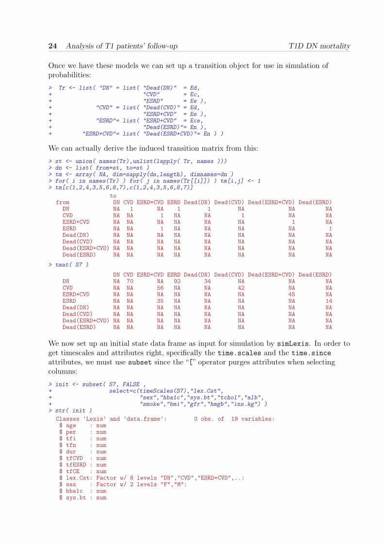
Once we have these models we can set up a transition object for use in simulation ofprobabilities:
> Tr <- list( "DN" = list( "Dead(DN)" = Ed,+ "CVD" = Ec,+ "ESRD" = Ee ),+ "CVD" = list( "Dead(CVD)" = Ed,+ "ESRD+CVD" = Ee ),+ "ESRD"= list( "ESRD+CVD" = Ece,+ "Dead(ESRD)"= En ),+ "ESRD+CVD"= list( "Dead(ESRD+CVD)"= En ) )
We can actually derive the induced transition matrix from this:
> st <- union( names(Tr),unlist(lapply( Tr, names )))> dn <- list( from=st, to=st )> tm <- array( NA, dim=sapply(dn,length), dimnames=dn )> for( i in names(Tr) ) for( j in names(Tr[[i]]) ) tm[i,j] <- 1> tm[c(1,2,4,3,5,6,8,7),c(1,2,4,3,5,6,8,7)]
tofrom DN CVD ESRD+CVD ESRD Dead(DN) Dead(CVD) Dead(ESRD+CVD) Dead(ESRD)DN NA 1 NA 1 1 NA NA NACVD NA NA 1 NA NA 1 NA NAESRD+CVD NA NA NA NA NA NA 1 NAESRD NA NA 1 NA NA NA NA 1Dead(DN) NA NA NA NA NA NA NA NADead(CVD) NA NA NA NA NA NA NA NADead(ESRD+CVD) NA NA NA NA NA NA NA NADead(ESRD) NA NA NA NA NA NA NA NA
> tmat( S7 )
DN CVD ESRD+CVD ESRD Dead(DN) Dead(CVD) Dead(ESRD+CVD) Dead(ESRD)DN NA 70 NA 92 34 NA NA NACVD NA NA 56 NA NA 42 NA NAESRD+CVD NA NA NA NA NA NA 45 NAESRD NA NA 35 NA NA NA NA 14Dead(DN) NA NA NA NA NA NA NA NADead(CVD) NA NA NA NA NA NA NA NADead(ESRD+CVD) NA NA NA NA NA NA NA NADead(ESRD) NA NA NA NA NA NA NA NA
We now set up an initial state data frame as input for simulation by simLexis. In order toget timescales and attributes right, specifically the time.scales and the time.since
attributes, we must use subset since the “[” operator purges attributes when selectingcolumns:
> init <- subset( S7, FALSE ,+ select=c(timeScales(S7),"lex.Cst",+ "sex","hba1c","sys.bt","tchol","alb",+ "smoke","bmi","gfr","hmgb","ins.kg") )> str( init )
Classes 'Lexis' and 'data.frame': 0 obs. of 19 variables:$ age : num$ per : num$ tfi : num$ tfn : num$ dur : num$ tfCVD : num$ tfESRD : num$ tfCE : num$ lex.Cst: Factor w/ 8 levels "DN","CVD","ESRD+CVD",..:$ sex : Factor w/ 2 levels "F","M":$ hba1c : num$ sys.bt : num
Analysis of T1 patients’ follow-up 1.2 Prediction of life course 25
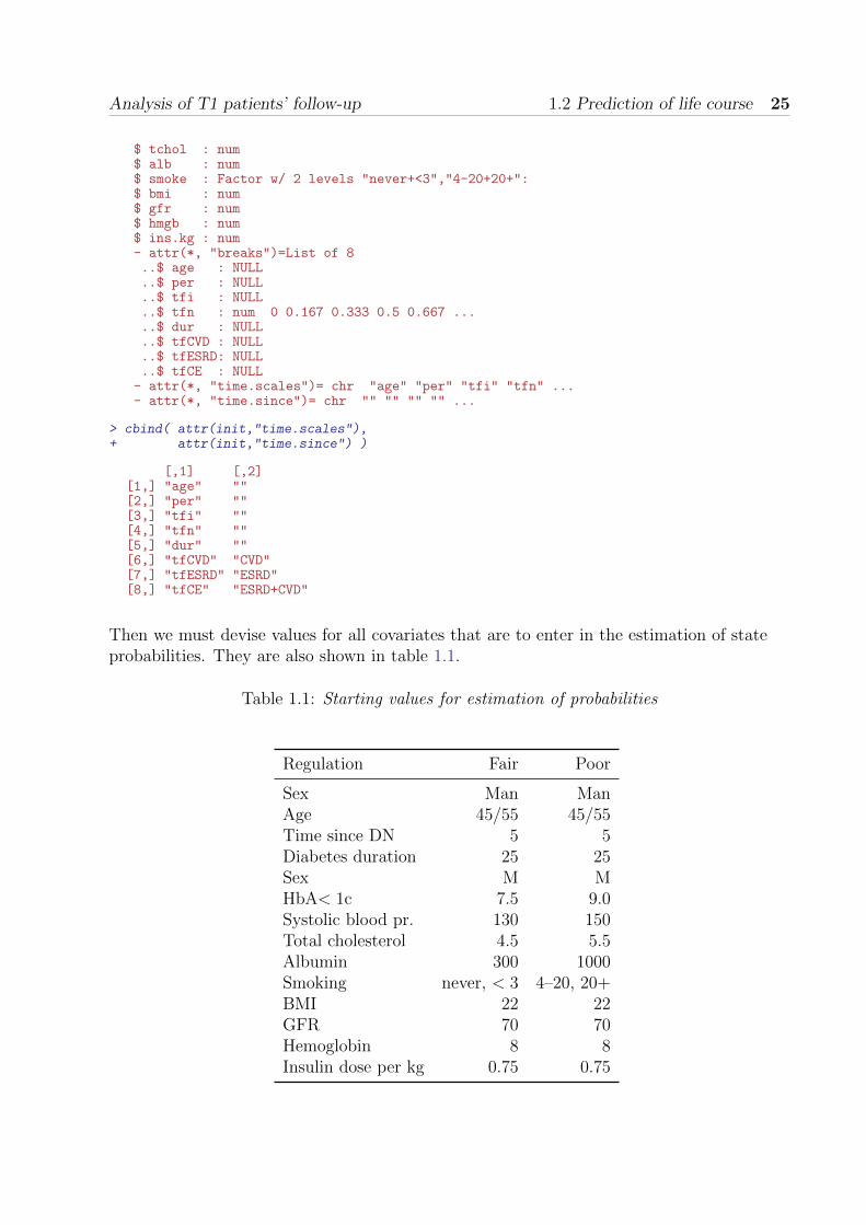
$ tchol : num$ alb : num$ smoke : Factor w/ 2 levels "never+<3","4-20+20+":$ bmi : num$ gfr : num$ hmgb : num$ ins.kg : num- attr(*, "breaks")=List of 8..$ age : NULL..$ per : NULL..$ tfi : NULL..$ tfn : num 0 0.167 0.333 0.5 0.667 .....$ dur : NULL..$ tfCVD : NULL..$ tfESRD: NULL..$ tfCE : NULL- attr(*, "time.scales")= chr "age" "per" "tfi" "tfn" ...- attr(*, "time.since")= chr "" "" "" "" ...
> cbind( attr(init,"time.scales"),+ attr(init,"time.since") )
[,1] [,2][1,] "age" ""[2,] "per" ""[3,] "tfi" ""[4,] "tfn" ""[5,] "dur" ""[6,] "tfCVD" "CVD"[7,] "tfESRD" "ESRD"[8,] "tfCE" "ESRD+CVD"
Then we must devise values for all covariates that are to enter in the estimation of stateprobabilities. They are also shown in table 1.1.
Table 1.1: Starting values for estimation of probabilities
Regulation Fair Poor
Sex Man ManAge 45/55 45/55Time since DN 5 5Diabetes duration 25 25Sex M MHbA< 1c 7.5 9.0Systolic blood pr. 130 150Total cholesterol 4.5 5.5Albumin 300 1000Smoking never, < 3 4–20, 20+BMI 22 22GFR 70 70Hemoglobin 8 8Insulin dose per kg 0.75 0.75

26 Analysis of T1 patients’ follow-up T1D DN mortality
> init[1:2,"sex"] <- rep(levels(init$sex)[2],2)> init[1:2,"age"] <- c(45,45)> init[1:2,"tfn"] <- rep(5,2)> init[1:2,"dur"] <- c(25,25)> init[1:2,"lex.Cst"]<- rep("DN",2)> init[1:2,"hba1c"] <- c(7.5,9)> init[1:2,"sys.bt"] <- c(130,150)> init[1:2,"tchol"] <- c(4.5,5.5)> init[1:2,"alb"] <- c(3,10)*100> init[1:2,"smoke"] <- levels(init$smoke)[c(1,2)]> init[1:2,"bmi"] <- c(22,22)> init[1:2,"gfr"] <- 70> init[1:2,"hmgb"] <- 8> init[1:2,"ins.kg"] <- 0.75> init$regl <- factor(c("Fair","Poor"))> init
age per tfi tfn dur tfCVD tfESRD tfCE lex.Cst sex hba1c sys.bt tchol alb smoke bmi1 45 NA NA 5 25 NA NA NA DN M 7.5 130 4.5 300 never+<3 222 45 NA NA 5 25 NA NA NA DN M 9.0 150 5.5 1000 4-20+20+ 22gfr hmgb ins.kg regl
1 70 8 0.75 Fair2 70 8 0.75 Poor
A quick glance at figure 1.2 shows that a substantial part of the patients enter the studyafter CVD, and it is therefore of interest to see how these fare. Hence we make a duplicateversion of the init data set where the persons are assumed to start in the CVD state.Based on the distribution of age at entry into the study we also do the claculation for aperson aged 45, resp. 55. Thus we will simulate probabilities for 8 = 23 differentcombinations:
• age: 45/55, DN dur: 5/15, DM dur: 25/35
• regulation: Fair/Poor
• state: DN/CVD
Note we do not have to specify CVD duration as this is not included in any of the models.DN duration will still exist as a time scale in the Lexis object but it will just be updated asNA during the iteration, and it has no effect since the variable is never used in any modelfor transitions subsequent to CVD.
> i.cvd <- transform( init, lex.Cst=factor("CVD",levels=levels(lex.Cst)) )> i.old <- transform( init, age=age+10,+ tfn=tfn+10,+ dur=dur+10 )> i.ocv <- transform( init, age=age+10,+ tfn=tfn+10,+ dur=dur+10,+ lex.Cst=factor("CVD",levels=levels(lex.Cst)) )> init <- rbind( init, i.cvd, i.old, i.ocv )> init$i.state <- init$lex.Cst> init$i.age <- init$age> init
age per tfi tfn dur tfCVD tfESRD tfCE lex.Cst sex hba1c sys.bt tchol alb smoke bmi1 45 NA NA 5 25 NA NA NA DN M 7.5 130 4.5 300 never+<3 222 45 NA NA 5 25 NA NA NA DN M 9.0 150 5.5 1000 4-20+20+ 223 45 NA NA 5 25 NA NA NA CVD M 7.5 130 4.5 300 never+<3 224 45 NA NA 5 25 NA NA NA CVD M 9.0 150 5.5 1000 4-20+20+ 225 55 NA NA 15 35 NA NA NA DN M 7.5 130 4.5 300 never+<3 226 55 NA NA 15 35 NA NA NA DN M 9.0 150 5.5 1000 4-20+20+ 227 55 NA NA 15 35 NA NA NA CVD M 7.5 130 4.5 300 never+<3 22

Analysis of T1 patients’ follow-up 1.2 Prediction of life course 27
8 55 NA NA 15 35 NA NA NA CVD M 9.0 150 5.5 1000 4-20+20+ 22gfr hmgb ins.kg regl i.state i.age
1 70 8 0.75 Fair DN 452 70 8 0.75 Poor DN 453 70 8 0.75 Fair CVD 454 70 8 0.75 Poor CVD 455 70 8 0.75 Fair DN 556 70 8 0.75 Poor DN 557 70 8 0.75 Fair CVD 558 70 8 0.75 Poor CVD 55
Now we can simulate transitions through the defined model for a specified number ofpatients with these patterns of initial values. Since simulation of 10,000 patients in one gowould be too much, we simulate in chunks of 500 replicates of each type of patient:
> NN <- 500> system.time(+ simL <- simLexis( Tr, init,+ time.pts=seq(0,15.2,0.2), N=NN )+ )
user system elapsed25.51 2.41 28.27
> summary( simL )
Transitions:To
From DN CVD ESRD+CVD ESRD Dead(DN) Dead(CVD) Dead(ESRD+CVD) Dead(ESRD) Records:DN 624 428 0 723 225 0 0 0 2000CVD 0 772 996 0 0 660 0 0 2428ESRD+CVD 0 0 471 0 0 0 868 0 1339ESRD 0 0 343 230 0 0 0 150 723Sum 624 1200 1810 953 225 660 868 150 6490
Transitions:To
From Events: Risk time: Persons:DN 1376 17852.83 2000CVD 1656 20636.92 2428ESRD+CVD 868 5248.99 1339ESRD 493 3257.10 723Sum 4393 46995.84 4000
We can then simulate another 19 times to get a sample of 10,000 simulated patients foreach of the 8 types of initial persons:
> system.time(+ for( i in 1:19 )+ {+ simL <- rbind( simL, simLexis( Tr, init,+ time.pts=seq(0,15.2,0.2), N=NN,+ lex.id=i*(NN*nrow(init))+1:(NN*nrow(init)) ) )+ cat( "Iter ", i, "at", strftime(Sys.time(),"%Y-%m-%d, %H:%M:%S"), "\n" )+ flush.console()+ } )
Iter 1 at 2014-01-01, 21:04:04Iter 2 at 2014-01-01, 21:04:31Iter 3 at 2014-01-01, 21:04:57Iter 4 at 2014-01-01, 21:05:24Iter 5 at 2014-01-01, 21:05:50Iter 6 at 2014-01-01, 21:06:17Iter 7 at 2014-01-01, 21:06:44Iter 8 at 2014-01-01, 21:07:12Iter 9 at 2014-01-01, 21:07:40Iter 10 at 2014-01-01, 21:08:08

28 Analysis of T1 patients’ follow-up T1D DN mortality
Iter 11 at 2014-01-01, 21:08:36Iter 12 at 2014-01-01, 21:09:04Iter 13 at 2014-01-01, 21:09:32Iter 14 at 2014-01-01, 21:10:01Iter 15 at 2014-01-01, 21:10:31Iter 16 at 2014-01-01, 21:11:00Iter 17 at 2014-01-01, 21:11:29Iter 18 at 2014-01-01, 21:11:58Iter 19 at 2014-01-01, 21:12:28
user system elapsed523.10 5.60 529.48
We then save the simulated data for possible future use:
> save( simL, file="./data/simL1.Rda" )> load( file="./data/simL1.Rda" )
We now have a data frame (a Lexis-object) with the lifecourse of 80,000 persons — 10,000for each combination of variables, and thus with somewhat more records:
> dim( simL )
[1] 129451 26
> summary( simL )
Transitions:To
From DN CVD ESRD+CVD ESRD Dead(DN) Dead(CVD) Dead(ESRD+CVD) Dead(ESRD)DN 12780 8094 0 14629 4497 0 0 0CVD 0 15382 19740 0 0 12972 0 0ESRD+CVD 0 0 9812 0 0 0 16916 0ESRD 0 0 6988 4515 0 0 0 3126Sum 12780 23476 36540 19144 4497 12972 16916 3126
Transitions:To
From Records: Events: Risk time: Persons:DN 40000 27220 362432.22 40000CVD 48094 32712 410801.93 48094ESRD+CVD 26728 16916 106142.72 26728ESRD 14629 10114 65389.53 14629Sum 129451 86962 944766.39 80000
> with( simL, ftable(regl,i.age,i.state) )
i.state DN CVD ESRD+CVD ESRD Dead(DN) Dead(CVD) Dead(ESRD+CVD) Dead(ESRD)regl i.ageFair 45 14401 12091 0 0 0 0 0 0
55 15096 13150 0 0 0 0 0 0Poor 45 21011 15101 0 0 0 0 0 0
55 22220 16381 0 0 0 0 0 0
Once we have the simulated Lexis objects we can compute the state occupancyprobabilities. We want to show these in different displays, so it is most convenient to collectthe estimated fractions in a large array, suitably indexing the dimensions of the array:
> times <- seq(0,15.2,0.1)> perm <- c(1:4,8:5)> levels( simL$lex.Cst )[perm]
[1] "DN" "CVD" "ESRD+CVD" "ESRD" "Dead(ESRD)"[6] "Dead(ESRD+CVD)" "Dead(CVD)" "Dead(DN)"
> pArr <- NArray( list( i.age = c(45,55),+ regl = c("Fair","Poor"),+ i.state = c("DN","CVD"),+ times = times,+ state = levels( simL$lex.Cst )[perm] ) )> dimnames( pArr )[-4]
Analysis of T1 patients’ follow-up 1.2 Prediction of life course 29
$i.age[1] "45" "55"
$regl[1] "Fair" "Poor"
$i.state[1] "DN" "CVD"
$state[1] "DN" "CVD" "ESRD+CVD" "ESRD" "Dead(ESRD)"[6] "Dead(ESRD+CVD)" "Dead(CVD)" "Dead(DN)"
> for( ia in dimnames(pArr)$i.age )+ for( ir in dimnames(pArr)$regl )+ for( ii in dimnames(pArr)$i.state )+ pArr[ia,ir,ii,,] <- pState( nState( subset( simL, i.age==as.numeric(ia) &+ regl==ir &+ i.state==ii ),+ at = times,+ from = as.numeric(ia),+ time.scale = "age" ),+ perm = perm )> save( pArr, file="./data/simP1.Rda" )
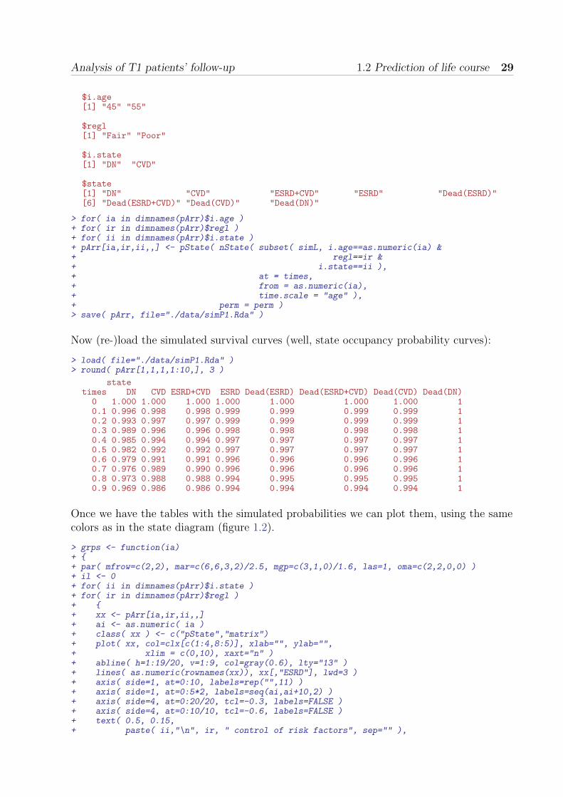
Now (re-)load the simulated survival curves (well, state occupancy probability curves):
> load( file="./data/simP1.Rda" )> round( pArr[1,1,1,1:10,], 3 )
statetimes DN CVD ESRD+CVD ESRD Dead(ESRD) Dead(ESRD+CVD) Dead(CVD) Dead(DN)0 1.000 1.000 1.000 1.000 1.000 1.000 1.000 10.1 0.996 0.998 0.998 0.999 0.999 0.999 0.999 10.2 0.993 0.997 0.997 0.999 0.999 0.999 0.999 10.3 0.989 0.996 0.996 0.998 0.998 0.998 0.998 10.4 0.985 0.994 0.994 0.997 0.997 0.997 0.997 10.5 0.982 0.992 0.992 0.997 0.997 0.997 0.997 10.6 0.979 0.991 0.991 0.996 0.996 0.996 0.996 10.7 0.976 0.989 0.990 0.996 0.996 0.996 0.996 10.8 0.973 0.988 0.988 0.994 0.995 0.995 0.995 10.9 0.969 0.986 0.986 0.994 0.994 0.994 0.994 1
Once we have the tables with the simulated probabilities we can plot them, using the samecolors as in the state diagram (figure 1.2).
> grps <- function(ia)+ {+ par( mfrow=c(2,2), mar=c(6,6,3,2)/2.5, mgp=c(3,1,0)/1.6, las=1, oma=c(2,2,0,0) )+ il <- 0+ for( ii in dimnames(pArr)$i.state )+ for( ir in dimnames(pArr)$regl )+ {+ xx <- pArr[ia,ir,ii,,]+ ai <- as.numeric( ia )+ class( xx ) <- c("pState","matrix")+ plot( xx, col=clx[c(1:4,8:5)], xlab="", ylab="",+ xlim = c(0,10), xaxt="n" )+ abline( h=1:19/20, v=1:9, col=gray(0.6), lty="13" )+ lines( as.numeric(rownames(xx)), xx[,"ESRD"], lwd=3 )+ axis( side=1, at=0:10, labels=rep("",11) )+ axis( side=1, at=0:5*2, labels=seq(ai,ai+10,2) )+ axis( side=4, at=0:20/20, tcl=-0.3, labels=FALSE )+ axis( side=4, at=0:10/10, tcl=-0.6, labels=FALSE )+ text( 0.5, 0.15,+ paste( ii,"\n", ir, " control of risk factors", sep="" ),

30 Analysis of T1 patients’ follow-up T1D DN mortality
+ col="white", font=2, adj=c(0,0) )+ box(col="white")+ mtext(letters[il<-il+1],line=0.2,adj=0)+ }+ mtext( "Probability", side=2, line=0, outer=TRUE, las=0 )+ mtext( "Age at follow-up", side=1, line=0, outer=TRUE )+ }
> grps("45")
> grps("55")
Also, we want to see the numerical size of some of the cumulative risks at 5, 10 and 15years after DN, specifically:
• cumulative risks of any ESRD (red and orange areas)
• cumulative risks of death (the survival curve))
• fraction of those acquiring ESRD that are dead (pale red and orange areas relative tototal red and orange areas)
So we set up an array to hold these quantities for the 8 types of T1 patients that we areconsidering:
> times <- c(5,10,15)> CumR <- NArray( c( dimnames( pArr )[1:3],+ list( when = times,+ what = c("cr-Death","cr-ESRD","pr-ESRDdead") ) ) )> str( CumR )
logi [1:2, 1:2, 1:2, 1:3, 1:3] NA NA NA NA NA NA ...- attr(*, "dimnames")=List of 5..$ i.age : chr [1:2] "45" "55"..$ regl : chr [1:2] "Fair" "Poor"..$ i.state: chr [1:2] "DN" "CVD"..$ when : chr [1:3] "5" "10" "15"..$ what : chr [1:3] "cr-Death" "cr-ESRD" "pr-ESRDdead"
> tms <- dimnames(CumR)$when
— and then extract the quantities at these specified times:
> CumR[,,,,"cr-Death"] <- 1-pArr[,,,tms,"ESRD"]> CumR[,,,,"cr-ESRD" ] <- pArr[,,,tms,"Dead(ESRD+CVD)"]-+ pArr[,,,tms,"CVD"]> CumR[,,,,"pr-ESRDdead" ] <- (pArr[,,,tms,"Dead(ESRD+CVD)"]-+ pArr[,,,tms,"ESRD"])/+ (pArr[,,,tms,"Dead(ESRD+CVD)"]-+ pArr[,,,tms,"CVD" ])
Finally we can show the cumulative risks in two different lay-outs:
> round( 100*ftable( CumR, col.vars=3:4 ), 1 )
i.state DN CVDwhen 5 10 15 5 10 15
i.age regl what45 Fair cr-Death 4.4 11.2 19.3 10.7 22.8 35.3
cr-ESRD 5.8 13.2 20.5 6.3 13.6 20.6pr-ESRDdead 16.1 30.8 43.1 33.9 51.3 62.9
Poor cr-Death 12.8 31.7 50.4 24.2 48.1 66.9

Analysis of T1 patients’ follow-up 1.2 Prediction of life course 31
0.0
0.2
0.4
0.6
0.8
1.0
45 47 49 51 53 55
DNFair control of risk factors
a
0.0
0.2
0.4
0.6
0.8
1.0
45 47 49 51 53 55
DNPoor control of risk factors
b
0.0
0.2
0.4
0.6
0.8
1.0
45 47 49 51 53 55
CVDFair control of risk factors
c
0.0
0.2
0.4
0.6
0.8
1.0
45 47 49 51 53 55
CVDPoor control of risk factors
d
Pro
babi
lity
Age at follow−up
Figure 1.9: Estimated probabilities of being in different states for patients shown in table 1.1,for T1 patients enterin at age 45. Coloring as in figure 1.2. The black line is the survivalcurve, the (pale) states above the line are the death states.

32 Analysis of T1 patients’ follow-up T1D DN mortality
0.0
0.2
0.4
0.6
0.8
1.0
55 57 59 61 63 65
DNFair control of risk factors
a
0.0
0.2
0.4
0.6
0.8
1.0
55 57 59 61 63 65
DNPoor control of risk factors
b
0.0
0.2
0.4
0.6
0.8
1.0
55 57 59 61 63 65
CVDFair control of risk factors
c
0.0
0.2
0.4
0.6
0.8
1.0
55 57 59 61 63 65
CVDPoor control of risk factors
d
Pro
babi
lity
Age at follow−up
Figure 1.10: Estimated probabilities of being in different states for patients shown in table1.1, for T1 patients enterin at age 55. Coloring as in figure 1.2. The black line is the survivalcurve, the (pale) states above the line are the death states.
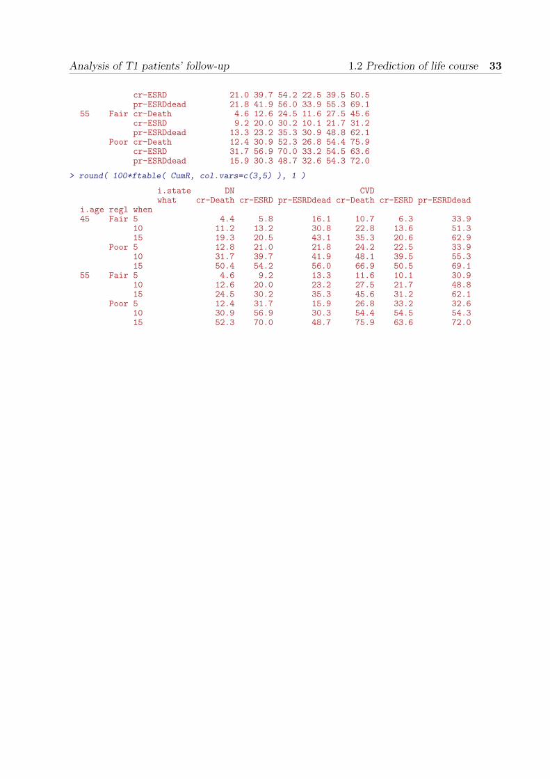
Analysis of T1 patients’ follow-up 1.2 Prediction of life course 33
cr-ESRD 21.0 39.7 54.2 22.5 39.5 50.5pr-ESRDdead 21.8 41.9 56.0 33.9 55.3 69.1
55 Fair cr-Death 4.6 12.6 24.5 11.6 27.5 45.6cr-ESRD 9.2 20.0 30.2 10.1 21.7 31.2pr-ESRDdead 13.3 23.2 35.3 30.9 48.8 62.1
Poor cr-Death 12.4 30.9 52.3 26.8 54.4 75.9cr-ESRD 31.7 56.9 70.0 33.2 54.5 63.6pr-ESRDdead 15.9 30.3 48.7 32.6 54.3 72.0
> round( 100*ftable( CumR, col.vars=c(3,5) ), 1 )
i.state DN CVDwhat cr-Death cr-ESRD pr-ESRDdead cr-Death cr-ESRD pr-ESRDdead
i.age regl when45 Fair 5 4.4 5.8 16.1 10.7 6.3 33.9
10 11.2 13.2 30.8 22.8 13.6 51.315 19.3 20.5 43.1 35.3 20.6 62.9
Poor 5 12.8 21.0 21.8 24.2 22.5 33.910 31.7 39.7 41.9 48.1 39.5 55.315 50.4 54.2 56.0 66.9 50.5 69.1
55 Fair 5 4.6 9.2 13.3 11.6 10.1 30.910 12.6 20.0 23.2 27.5 21.7 48.815 24.5 30.2 35.3 45.6 31.2 62.1
Poor 5 12.4 31.7 15.9 26.8 33.2 32.610 30.9 56.9 30.3 54.4 54.5 54.315 52.3 70.0 48.7 75.9 63.6 72.0

34 Analysis of T1 patients’ follow-up T1D DN mortality
Compilation logR 3.0.2---------------------------------------------Program: DN1.rnwFolder: c:\Bendix\Steno\GbAdStarted: onsdag 01. januar 2014, 21:02:15---------------------------------------------Writing to file DN1.texProcessing code chunks with options ...1 : echo keep.source term hide (T1nef.rnw:5)2 : echo keep.source term verbatim (T1nef.rnw:10)3 : echo keep.source term verbatim (T1nef.rnw:17)4 : echo keep.source term verbatim eps pdf (label = boxes-tp1, T1nef.rnw:92)5 : echo keep.source term verbatim (T1nef.rnw:114)6 : echo keep.source term verbatim (T1nef.rnw:123)7 : echo keep.source term verbatim (label = stack, T1nef.rnw:135)8 : echo keep.source term verbatim (label = subset-stack, T1nef.rnw:144)9 : echo keep.source term verbatim (label = m0, T1nef.rnw:158)10 : echo keep.source term verbatim (label = prop-tests, T1nef.rnw:181)11 : echo keep.source term verbatim (T1nef.rnw:210)12 : echo keep.source term verbatim (label = m1-m2-cov, T1nef.rnw:281)13 : echo keep.source term verbatim (label = base-separate, T1nef.rnw:308)14 : echo keep.source term verbatim (T1nef.rnw:315)15 : echo keep.source term verbatim (T1nef.rnw:325)16 : echo keep.source term verbatim eps pdf (label = base-CVD1, T1nef.rnw:355)17 : echo keep.source term verbatim (label = RR-comp-mort1, T1nef.rnw:382)18 : echo keep.source term verbatim (label = RR-comp-ESRD, T1nef.rnw:393)19 : echo keep.source term verbatim eps pdf (label = xforest1, T1nef.rnw:411)20 : echo keep.source term verbatim eps pdf (label = xforestcol1, T1nef.rnw:456)21 : echo keep.source term verbatim eps pdf (label = pairs1, T1nef.rnw:492)22 : echo keep.source term verbatim (label = covariaate-medians, T1nef.rnw:506)23 : echo keep.source term verbatim (label = used-values, T1nef.rnw:517)24 : echo keep.source term verbatim (label = pred-frames, T1nef.rnw:523)25 : echo keep.source term verbatim (label = get-rates, T1nef.rnw:560)26 : echo keep.source term verbatim (label = plr-def, T1nef.rnw:579)27 : echo keep.source term verbatim eps pdf (label = crates, T1nef.rnw:597)28 : echo keep.source term verbatim eps pdf (label = rates, T1nef.rnw:611)29 : echo keep.source term verbatim (T1nef.rnw:642)30 : echo keep.source term verbatim (label = per-eff, T1nef.rnw:655)31 : echo keep.source term verbatim (T1nef.rnw:690)32 : echo keep.source term verbatim (T1pred.rnw:15)33 : echo keep.source term verbatim (T1pred.rnw:20)34 : echo keep.source term verbatim (T1pred.rnw:30)35 : echo keep.source term verbatim (T1pred.rnw:41)36 : echo keep.source term verbatim (T1pred.rnw:53)37 : echo keep.source term verbatim (T1pred.rnw:64)38 : echo keep.source term verbatim (T1pred.rnw:77)39 : echo keep.source term verbatim (T1pred.rnw:114)40 : echo keep.source term verbatim (T1pred.rnw:150)41 : echo keep.source term verbatim (label = sim1st, T1pred.rnw:168)42 : echo keep.source term verbatim (label = simrest, T1pred.rnw:178)43 : echo keep.source term verbatim (T1pred.rnw:190)44 : echo keep.source term verbatim (T1pred.rnw:197)45 : echo keep.source term verbatim (label = Gen-Surv, T1pred.rnw:206)46 : echo keep.source term verbatim (label = Get-surv, T1pred.rnw:230)47 : echo keep.source term verbatim (label = defpl, T1pred.rnw:237)48 : echo keep.source term verbatim eps pdf (label = pr45, T1pred.rnw:266)49 : echo keep.source term verbatim eps pdf (label = pr55, T1pred.rnw:269)50 : echo keep.source term verbatim (T1pred.rnw:294)51 : echo keep.source term verbatim (T1pred.rnw:303)52 : echo keep.source term verbatim (T1pred.rnw:313)
You can now run (pdf)latex on 'DN1.tex'
---------------------------------------------Program: DN1.rnwFolder: c:\Bendix\Steno\GbAdEnded: onsdag 01. januar 2014, 21:13:58
Elapsed: 00:11:43---------------------------------------------