MODEL BASED VISUAL RELATIVE MOTIONESTIMATION AND CONTROL OF A SPACECRAFT

UTILIZING COMPUTER GRAPHICS

Fuyuto Terui

Japan Aerospace Exploration Agency7-44-1 Jindaiji-Higashimachi, Chofu-shi, Tokyo 182-8522, JAPAN

TEL : 81-422-40-3164E-mail : terui.fuyuto@jaxa.jp

Abstract

An algorithm is developed for estimating the motion (relative attitude and rela-tive position) of large pieces of space debris, such as failed satellite. The algorithm isdesigned to be used by a debris removal space robot which would perform six degree-of-freedom motion control (control its position and attitude simultaneously). Theinformation required as feedback signals for such a controller is relative–position,velocity, attitude and angular velocity–and these are expected to be measured or es-timated from image data. The algorithm uses a combination of stereo vision, 3D modelmatching, applying the ICP (Iterative Closest Point) algorithm, and extended KalmanFilter to increase the reliability of estimates. To evaluate the algorithm, a simulator isprepared to simulate the on-orbit optical environment in terrestrial experiments, andthe motion of a miniature satellite model is estimated using images obtained from thesimulator. In addition to that, six DOF(Degrees Of Freedom) manoeuvre simulationwith developed algorithm for motion estimation using image data was succefully triedfor the proximity flight around a failed satellite utilizing CG(Computer Graphics).

1 INTRODUCTION

As the number of satellites continues to increase, space debris is becoming an increasinglyserious problem for near-Earth space activities and effective measures to mitigate it areimportant. Satellite end-of-life de-orbiting and orbital lifetime reduction capability will beeffective in reducing the amount of debris by reducing the probability of collisions, but thisapproach cannot be applied to inert satellites and debris. On the other hand, a debris removalspace robot comprising of a spacecraft (“chaser”) that actively removes space debris andretrieves malfunctioned satellites (“targets”) is considered as a complementary approach.[6]The concept of such a removal space robot is shown in Fig. 1. After rendezvous with the

target and approach to approximately 50m using data from ground observations, satellitenavigation positioning and radar, the chaser maintains a constant distance from the targetmeasured using images taken by onboard cameras. During this station-keeping phase, thechaser captures images of the target to allow remote visual inspection and measures itsmotion by image processing both onboard and on the ground. Since the target is non-cooperative, there is no communication, no special markings or retro-reflectors to assist

1

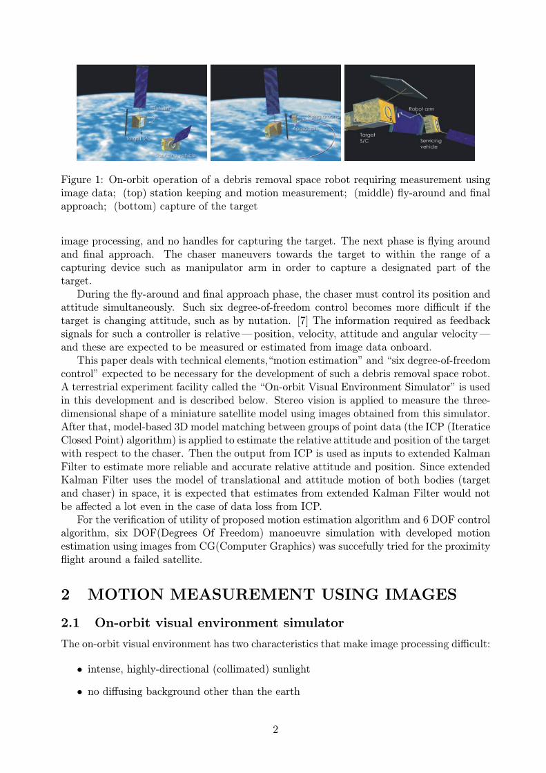
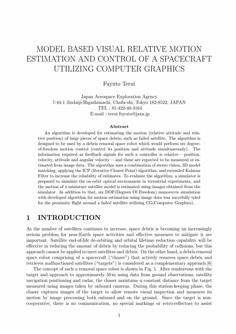
Figure 1: On-orbit operation of a debris removal space robot requiring measurement usingimage data; (top) station keeping and motion measurement; (middle) fly-around and finalapproach; (bottom) capture of the target

image processing, and no handles for capturing the target. The next phase is flying aroundand final approach. The chaser maneuvers towards the target to within the range of acapturing device such as manipulator arm in order to capture a designated part of thetarget.During the fly-around and final approach phase, the chaser must control its position and

attitude simultaneously. Such six degree-of-freedom control becomes more difficult if thetarget is changing attitude, such as by nutation. [7] The information required as feedbacksignals for such a controller is relative–position, velocity, attitude and angular velocity–and these are expected to be measured or estimated from image data onboard.This paper deals with technical elements,“motion estimation” and “six degree-of-freedom

control” expected to be necessary for the development of such a debris removal space robot.A terrestrial experiment facility called the “On-orbit Visual Environment Simulator” is usedin this development and is described below. Stereo vision is applied to measure the three-dimensional shape of a miniature satellite model using images obtained from this simulator.After that, model-based 3D model matching between groups of point data (the ICP (IteraticeClosed Point) algorithm) is applied to estimate the relative attitude and position of the targetwith respect to the chaser. Then the output from ICP is used as inputs to extended KalmanFilter to estimate more reliable and accurate relative attitude and position. Since extendedKalman Filter uses the model of translational and attitude motion of both bodies (targetand chaser) in space, it is expected that estimates from extended Kalman Filter would notbe affected a lot even in the case of data loss from ICP.For the verification of utility of proposed motion estimation algorithm and 6 DOF control

algorithm, six DOF(Degrees Of Freedom) manoeuvre simulation with developed motionestimation using images from CG(Computer Graphics) was succefully tried for the proximityflight around a failed satellite.

2 MOTION MEASUREMENT USING IMAGES

2.1 On-orbit visual environment simulator

The on-orbit visual environment has two characteristics that make image processing difficult:

• intense, highly-directional (collimated) sunlight

• no diffusing background other than the earth

2

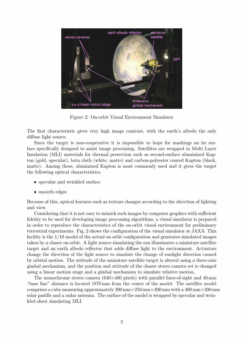
Figure 2: On-orbit Visual Environment Simulator

The first characteristic gives very high image contrast, with the earth’s albedo the onlydiffuse light source.Since the target is non-cooperative it is impossible to hope for markings on its sur-

face specifically designed to assist image processing. Satellites are wrapped in Multi LayerInsulation (MLI) materials for thermal protection such as second-surface aluminized Kap-ton (gold, specular), beta cloth (white, matte) and carbon-polyester coated Kapton (black,matte). Among these, aluminized Kapton is most commonly used and it gives the targetthe following optical characteristics.

• specular and wrinkled surface

• smooth edges

Because of this, optical features such as texture changes according to the direction of lightingand view.Considering that it is not easy to mimick such images by computer graphics with sufficient

fidelity to be used for developing image processing algorithms, a visual simulator is preparedin order to reproduce the characteristics of the on-orbit visual environment for preliminaryterrestrial experiments. Fig. 2 shows the configuration of the visual simulator at JAXA. Thisfacility is the 1/10 model of the actual on orbit configuration and generates simulated imagestaken by a chaser on-orbit. A light source simulating the sun illuminates a miniature satellitetarget and an earth albedo reflector that adds diffuse light to the environment. Actuatorschange the direction of the light source to simulate the change of sunlight direction causedby orbital motion. The attitude of the miniature satellite target is altered using a three-axisgimbal mechanism, and the position and attitude of the chaser stereo camera set is changedusing a linear motion stage and a gimbal mechanism to simulate relative motion.The monochrome stereo camera (640×480 pixels) with parallel lines-of-sight and 40mm

“base line” distance is located 1870mm from the center of the model. The satellite modelcomprises a cube measuring approximately 300mm×250mm×200mm with a 400mm×200mmsolar paddle and a radar antenna. The surface of the model is wrapped by specular and wrin-kled sheet simulating MLI.

3

Figure 3: (top-left)A Motion Estimation using On-orbit Visual Environment Simulator,(top-right)Motion Estimation utilizing CG, (bottom-left)6-DOF manoeuvre simulation withmotion estimation utilizing CG, (bottom-right)Hardware-In the Loop simulation for 6-DOFmanoeuvre

2.2 Motion estimation algorithm

Various researchers have investigated image processing techniques for measuring the motionof targets in the space environment. Their methods vary depending upon their researchobjectives and assumptions. [4], [5], [1])For this paper, we sought a strategy that would be able to use 3D shape information

obtained from ordinary image data and that would not be affected by data loss from shad-ows, occulusion or specular reflection. [8] Fig. 4 shows our strategy for motion measurementapplying to the experiment of fig. 3 : top-left. The area-based stereo matching algorithmgives 3D position data for the viewable area of the satellite model’s surface from a pair ofcameras, but since the only limited area of the model is in view at any one instant, andthe appearance of the area changes according to the model’s attitude and the direction ofillumination, the number of measured points obtained tends to be limited. The stereo match-ing algorithm also gives many incorrectly measured points due to matching failures, furtherreducing the number of accurately measured points obtained. However, it is assumed thatthe geometry of the satellite can be obtained from design data, and so a three-dimensionalshape model of the target may be constructed a priori and model matching can be appliedbetween this model and the 3D measurement points obtained from stereo matching, allowingrelative position and relative attitude to be estimated. A matching algorithm called the ICP

4

Figure 4: A Motion Estimation Strategy using Image

(Iterative Closest Point) algorithm is used for this purpose. Using measured relative posi-tion and attitude as a input, extended Kalman Filter outputs estimated these values withreduced noise and increased reliability. Extended Kalman Filter output predicted relativeposition and attitude as well as estimated ones. These are used for pre-alignment and frontsurface generation which is used as a model 3D points in the process of ICP resulting goodmatching result.

2.3 Stereo vision

The area-based stereo vision algorithm uses multiple images taken from different viewpointsand generates a 3D disparity map which contains displacement information between thecameras and points on the object. The final output of the algorithm is the 3D shape of thepart of the object in view reconstructed from the disparity map. In the area-based stereomethod, a small window (e.g. 17×17 pixels) around each pixel in the image is matched using“texture”; i.e. by minimizing an image similarity function such as SAD (Sum of AbsoluteDifferences) of pixel intensities, defined as follows:

QSAD (I, J, d(I, J)) =N1X

p=−N1

N2Xq=−N2

|F1(I + p, J + q, d)−G0(I + p, J + q)| (1)

F1(I, J, d) = G1 (I + d, J) . (2)

where the size of the matching window is (2N1 + 1) × (2N2 + 1). G0(I, J) is the intensityof a pixel in the reference camera image (left camera) and G1(I, J) is the intensity of thecorresponding pixel in the right camera image. d(I, J) is the disparity, which is the positionaldifference of the corresponding point from the reference point, and this should be optimizedto minimize QSAD(I, J, d) for each unit pixel. F1(I, J, d) in eq.(2) is the pixel intensity ofa point (I + d, J) in G1 which is a candidate for the corresponding point to G0(I, J). Itshould be noted that since the pair of cameras used are aligned side-by-side with parallellines-of-sight, the epipolar line for finding the matching window in the right camera image

5

Figure 5: Mmeasured 3D points by stereo vision

will be parallel to the horizontal image axis. Therefore, d appears only in the horizontalimage coordinate of G1 in eq.(2). The optimized disparities d

∗(I, J)

d∗(I, J) = argdminQSAD (I, J, d(I, J)) (3)

are then obtained for all pixels in G0, and make up the disparity map. To pre-processimages for stereo matching, the LoG (Laplacian of Gaussian) filter, which is a spatial bandpass filter, is used for extracting and enhancing specific features in image. Fig. 5 showsan example of the result of applying the stereo vision algorithm to a satellite model withspecular reflection. The attitude of the miniature satellite is fixed and the stereo camerais located 1870mm from the center of the model. The satellite model comprises a cubemeasuring approximately 300mm×250mm×200mm with a 400mm×200mm solar paddleand a 320mm×150mm radar antenna. A pair of digital CCD cameras with resolution of640×480 pixels are used. The left pictures in fig. 5 show the images taken by each cameraafter compensation of lens distortion. It is quite difficult to notice the difference betweenthem at first glance, but differences in the horizontal position between corresponding parts(disparity) can be observed. The right of the figure shows measured 3D points.The original 3D points have lots of spurious noise-like “outliers” sprinkled around the

satellite shape. Some of these are from the albedo reflector, the background curtain behindthe model and the 3-axis gimbal mechanism beneath the model. The dots from the reflectorand the curtain were removed using 3D position thresholding. The dots from the gimbalmechanism were suppressed by wrapping it using matte black cloths. Other noisy spuriouspoints appear as if they were sprayed from the position of the camera and these are thought tobe points where the stereo vision algorithm failed to find a matching window using texture fordetermining disparity. These are eliminated by Curvature masking, Left-Right ConsistencyChecking and Median Filtering. It can be seen that 3D point positions are obtained for onlya limited part of the model.

2.4 ICP algorithm

Fig. 6 shows the computational flow of the ICP algorithm.[3] The superscript (m) showsiteration number. This handles two point sets such as a measured data point set P and amodel data point set X(m). It first establishes correspondences between the data sets byfinding the closest point y(m)

iin X(m) for each point pi in P (the 3rd box). Next, it finds

the rotational transformation matrix R(m) and translational transformation matrix T (m) for

6

Figure 6: ICP algorithm

Y (m) which minimizes the cost function J shown in Fig. 6 (the 4th box). This cost function

is the summation of the distance between corresponding points pi and y(m)i . The algorithm

in Horn (Ref. [2]) gives closed-form solution for this problem using the eigenvalue problemand finally estimated relative position x, y, z which gives T and the estimated quaternionq which gives optimal R are directly calculated. X(m) and Y (m) are then transformed usingR(m) and T (m) (the 5th box). This process is repeated until convergence criteria E ≤ TE isachieved or iteration exceeds the threshold m ≥ Tm (the 6th and 7th box).

2.5 extended Kalman filter and front surface model

The simple and intuitive ICP algorithm has a number of advantages. Since it is an algorithmfor point sets, it is independent of shape representation and does not require any local featureextraction. It can also handle a reasonable amount of noise such as mismatched dots fromstereo vision.The main disadvantage of ICP alogorithm is that correct registration (matching) is not

guaranteed. Depending on the initial relative position and attitude between two point sets,the result of matching could fall into a local minimum. In order to prevent this, pre-alignmentof the model data set relative to the measured data set using some measure is required.The information used for the pre-alignment is predicted measurement given by extended

Kalman Filter. The state and measurement of extended Kalman Filter for position (Xp, Yp)and attitude (Xa, Ya) are as follows,

Xp =

"rHTCrHTC

#, Yp =

"rCCT∆rCCT

#(4)

7

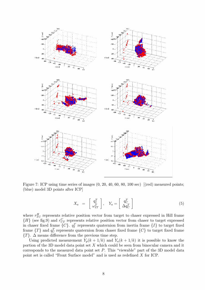
Figure 7: ICP using time series of images (0, 20, 40, 60, 80, 100 sec) [(red) measured points;(blue) model 3D points after ICP]

Xa =

"qTIωTIT

#, Ya =

"qTC∆qTC

#(5)

where rHTC represents relative position vector from target to chaser expressed in Hill frame{H} (see fig.9) and rCCT represents relative position vector from chaser to target expressedin chaser fixed frame {C}. qTI represents quaternion from inertia frame {I} to target fixedframe {T} and qTC represents quaternion from chaser fixed frame {C} to target fixed frame{T}. ∆ means difference from the previous time step.Using predicted measurement Yp(k + 1/k) and Ya(k + 1/k) it is possible to know the

portion of the 3D model data point set X which could be seen from binocular camera and itcorresponds to the measured data point set P . This “viewable” part of the 3D model datapoint set is called “Front Surface model” and is used as redefined X for ICP.

8

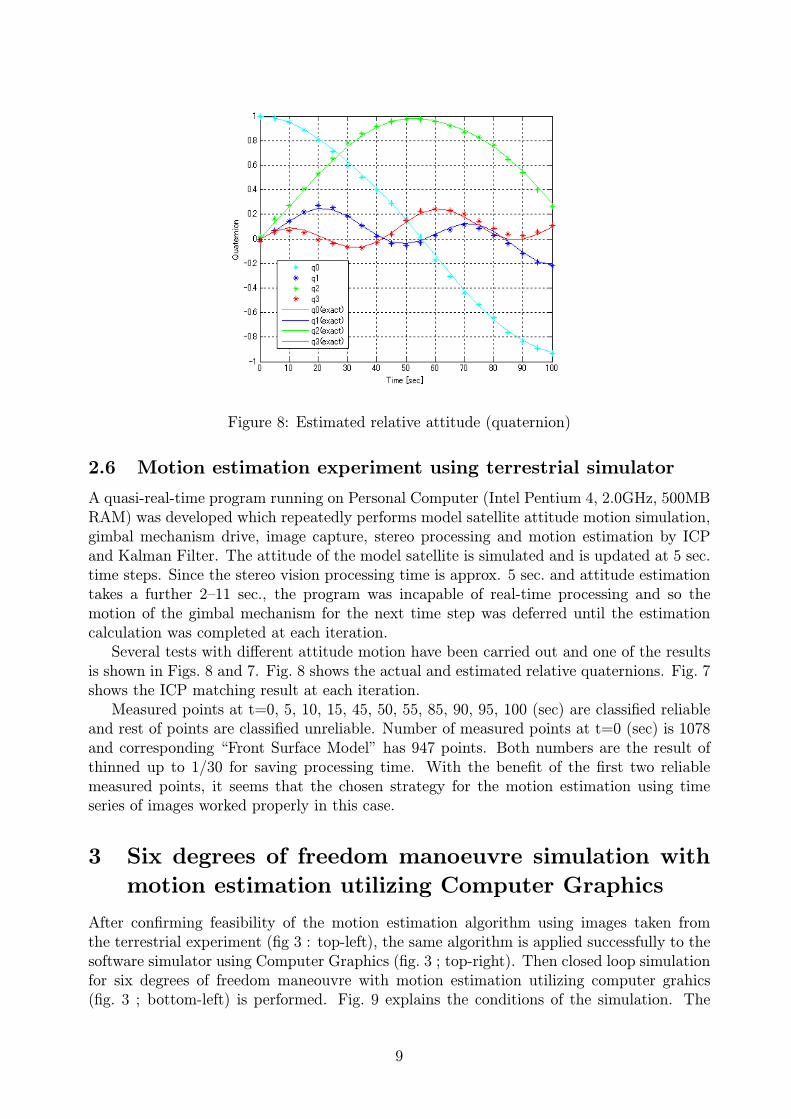
Figure 8: Estimated relative attitude (quaternion)

2.6 Motion estimation experiment using terrestrial simulator

A quasi-real-time program running on Personal Computer (Intel Pentium 4, 2.0GHz, 500MBRAM) was developed which repeatedly performs model satellite attitude motion simulation,gimbal mechanism drive, image capture, stereo processing and motion estimation by ICPand Kalman Filter. The attitude of the model satellite is simulated and is updated at 5 sec.time steps. Since the stereo vision processing time is approx. 5 sec. and attitude estimationtakes a further 2—11 sec., the program was incapable of real-time processing and so themotion of the gimbal mechanism for the next time step was deferred until the estimationcalculation was completed at each iteration.Several tests with different attitude motion have been carried out and one of the results

is shown in Figs. 8 and 7. Fig. 8 shows the actual and estimated relative quaternions. Fig. 7shows the ICP matching result at each iteration.Measured points at t=0, 5, 10, 15, 45, 50, 55, 85, 90, 95, 100 (sec) are classified reliable

and rest of points are classified unreliable. Number of measured points at t=0 (sec) is 1078and corresponding “Front Surface Model” has 947 points. Both numbers are the result ofthinned up to 1/30 for saving processing time. With the benefit of the first two reliablemeasured points, it seems that the chosen strategy for the motion estimation using timeseries of images worked properly in this case.

3 Six degrees of freedom manoeuvre simulation with

motion estimation utilizing Computer Graphics

After confirming feasibility of the motion estimation algorithm using images taken fromthe terrestrial experiment (fig 3 : top-left), the same algorithm is applied successfully to thesoftware simulator using Computer Graphics (fig. 3 ; top-right). Then closed loop simulationfor six degrees of freedom maneouvre with motion estimation utilizing computer grahics(fig. 3 ; bottom-left) is performed. Fig. 9 explains the conditions of the simulation. The

9

target is a failed satellite on Low Earth Orbit and the chaser is a “free flying” space robotwhich rendezvous to the target and flies in proximity to the target utilizing image data asmeasurement. {T}, {C} are coordinate frames fixed to the target and chaser respectivelyand {H} is Hill frame with the same origin as {T}. Both position and attitude controllerare designed applying sliding mode control. [7]

3.1 Position controller

The position control force obtained from sliding mode control is as follows,

F = −αpmSp

|Sp|+ ²p. (6)

where αp is a feedback gain, m is mass of chaser and ²p is small positive scalar for preventing”chattering. The switching surface Sp is defined

Sp = vCe + kp r

Ce . (7)

kp is a constant defining the switching surface. rCe and v

Ce in eq. (7) is relative position and

velocity between required point for position control and the center of chaser defined eq. (8),(9) below, as well as shown in fig. 9.

rCe = rCC − DC

T rTreq (8)

vCe = vCC − DC

T ωTIT rTreq (9)

where DCT is direction cosine matrix transforming from {T} to {C} and ωTIT is attitude rate

of the target. rCC , DCT , v

CC and ω

TIT are all estimated from image data.

3.2 Attitude controller

The sliding mode attitude control torque is

T = −αaISa

|Sa|+ ²a. (10)

where αa is a feedback gain, I is moment of inertia of chaser and ²a is small positive scalarfor preventing ”chattering. The switching surface Sa is defined as follows.

Sa = ωCe + ka1 qe vector sgn(qe vector) + ka2 qCT vector(2, 1) sgn(q

CT scalar) (11)

ka1 is a constant defining the switching surface. qe vector in eq. (11) is a quaternion repre-senting the error angle θLOS between LOS vector of the onboard camera rLOS and relativeposition vector beween target and chaser rC as shown in fig. 9. Since the major purpose forusing qe vector as feedback signal for attitude control is to minimize θLOS, there still remainsthe attitude error along the LOS axis. In order to make it small, qCT vector(2, 1) which repre-sents attitude error between {T} and {C} along rLOS is also used as a feedback signal fordefining switching surface.The process for calculating qe from rCC , r

CLOSis shown in eqs. (12)-(15). r

CC is given from

motion estimation using image data explained in previous section.

qe vector = λ sin

ÃθLOS2

!(12)

10

Figure 9: Target, chaser, frames, vectors

Figure 10: Time sequence of the proximity maneouvre

qe scalar = cos

ÃθLOS2

!(13)

λ = − rCC × rCLOS|rCC × rCLOS|

(14)

θLOS = arccos

Ã− rCC · rCLOS|rCC | |rCLOS|

!(15)

ωCe in eq. (11) is defined below. ωCC is from Gyros on chaser. As is the case of the position

control, DCT and ω

TIT are all estimated from motion estimation utilizing image data.

ωCe = ωCC − DCT ωTIT (16)

3.3 Numerical simulation

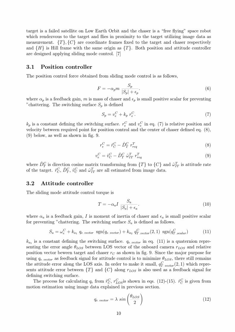
The time sequence of the proximity maneouvre is shown in fig.10 and table1. It is a proximitymaneouvre after rendezvous to the distance of approx.18 [m]. After the station keepingphase, it moves up for 10 [m] then moves back to the original position afterwards. Duringthis maneouvre the chaser controls its position so that its own center of mass to be coincidentwith the desired position in the target fixed frame {T} and controls its attitude so that theLOS of its onboard camera points to the mass center of the target. It is assumed that thetarget is not doing attitude motion. Images of the target was generated by CG(ComputerGraphics) and these are processed by motion estimation algorithm (Stereo vision + ICP +

11

Table 1: Time table of the proximity maneouvre

Table 2: Specifications of target(left) and chaser(right)

extended Kalman Filter). It is assumed that the direction of sunlight is in −YT axis directionso that it could be suitable for image capturing.Table2 shows specificatins of target and chaser. The chaser is designed as a micro satellite

with the mass of 3.59 [kg] and it has three wheels for attitude control and six thrusters forposition control.Fig.11-14 show the result of the simulation. It can be seen that the position of the chaser

is controlled with error of approx. ±3[m] in each direction. (see Figs.11 and 12) As is seenfrom fig. 12, it is speculated that the error is mainly due to the estimated relative positionerror in re caused by attitude control measurement and control error in D

CT . Fig.13 shows

the position of the center of the target in the FOV(Fiels Of View) of the chaser onboardcamera. It is controlled by the attitude controller to be within the area of FOV where motionestimation from image is possible.Fig.14 shows some examples of CG images of the left camera of binocular vision and

result of motion estimation algorithm. Blue points in the lower row shows measured pointsusing stereo vision and red points shows model 3D points after the matching by ICP(IterativeClosest Point) algorithm. The column at 5 [sec] shows the initial state, the column at 450[sec] shows the intermediate position moving from [0, 18, 0][m] to [0, 18, 10][m], the columnat 700 [sec] is at [0, 18, 10][m], the column at 750 [sec] is at the intermidiate position goingback to the initial position from [0, 18, 10][m] and the collumn at 1000 [sec] is at the initialposition. The image is captured every 5 [sec] and processed for motion estimation. It canbe seen that blue red points was matched to the blue points successfully generating relativeposition and attitude.

12

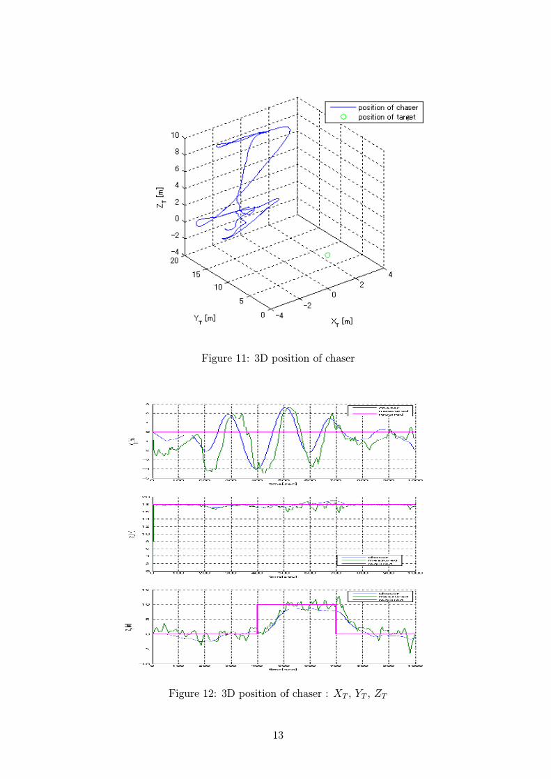
Figure 11: 3D position of chaser

Figure 12: 3D position of chaser : XT , YT , ZT

13

Figure 13: position of target in FOV

Figure 14: CG+measured model points

14

4 Concluding remarks and future work

Motion estimation of a large space debris object using image data was performed by applyingStereo Vision, the ICP(Iterative Closest Point) algorithm using a measured data point setand a model data point set, and extended Kalman Filter. Three-axis attitude motion andposition were estimated in a terrestrial experiment using an On-orbit Visual EnvironmentSimulator. Six DOF(Degrees Of Freedom) manoeuvre simulation with motion estimationbased on CG(Computer Graphics) applying developed algorithm was succefully tried for theproximity flight around a failed satellite.More challenging six DOF manoeuvre simulation such as for the chaser following nutating

satellite would be the next goal of this research. In addition to that, hardware In the Loopsimulation replacing the CG image by images taken in the ”On-orbit Visual EnvironmentSimulator”(fig. 3 : bottom-right) is now under preparation.

References

[1] A. Cropp and P. Palmer. Pose estimation and relative orbit determination of a nearbytarget microsatellite using passive imagery. 5th Cranfield Conference on Dynamics andControl of Systems and Structures in Space 2002, pages 389—395, 2002.

[2] B. K. P. Horn. Closed-form solution of absolute orientation using unit quaternions.Journal of Optical Society of America, 4-4:629—642, 1987.

[3] P. J.Besl and N. D.McKay. A method for registration of 3-d shapes. IEEE Transactionsof Pattern Analysis and Machine Intelligence, 14-2:239—256, 1992.

[4] M. D. Lichter and S. Dubowsky. Estimation of state, shape, and inertial parameters ofspace objects from sequences of range images. Proc. SPIE Vol. 5267 : Intelligent Robotsand Computer Vision XXI:Algorithms, Techniques, and Active Vision, D. P. Casasent,ed., pages 194—205, 2003.

[5] P. Jasiobedzki M. Abraham and M. Umasuthan. Robust 3d vision for autonomousspace robotic operation. Proceedings of the 6th International Symposium on ArtificialIntelligence and Robotics & Automation in Space : i-SAIRAS, June 18-22, 2001.

[6] S. Nishida. On-orbit servicing and assembly : Japanese perspective and more. Pro-ceedings of 24th International Symposium on Space Technology and Science, Miyazaki,JAPAN, 2004.

[7] F. Terui. Position and attitude control of a spacecraft by sliding mode control. Proceedingsof the American Control Conference, pages 217—221, 1998.

[8] F. Terui. Relative motion estimation and control to a failed satellite by machine vision.Space Technology, 27:90—96, 2007.

15BACK TO SESSION DETAILED CONTENTS BACK TO HIGHER LEVEL CONTENTS