estimation of relative permeability and...
TRANSCRIPT
ESTIMATION OF RELATIVE PERMEABILITY AND
CAPILLARY PRESSURE FOR HYDROCARBON RESERVOIRS
USING ENSEMBLE-BASED HISTORY MATCHING TECHNIQUES
A Thesis
Submitted to the Faculty of Graduate Studies and Research
In Partial Fulfillment of the Requirements
For the Degree of
Doctor of Philosophy
In
Petroleum Systems Engineering
University of Regina
By
Yin Zhang
Regina, Saskatchewan
July, 2014
Copyright 2014: Y. Zhang

UNIVERSITY OF REGINA
FACULTY OF GRADUATE STUDIES AND RESEARCH
SUPERVISORY AND EXAMINING COMMITTEE
Yin Zhang, candidate for the degree of Doctor of Philosophy in Petroleum Systems Engineering, has presented a thesis titled, Estimation of Relative Permeability and Capillary Pressure for Hydrocarbon Reservoirs Using Ensemble-Based History Matching Techniques, in an oral examination held on May 22, 2014. The following committee members have found the thesis acceptable in form and content, and that the candidate demonstrated satisfactory knowledge of the subject material. External Examiner: *Dr. Chaodong Yang, Computer Modelling Group Ltd
Supervisor: Dr. Daoyong Yang, Petroleum Systems Engineering
Committee Member: Dr. Farshid Torabi, Petroleum Systems Engineering
Committee Member: Dr. Malcolm Wilson, Adjunct
Committee Member: Dr. Stephen Bend, Department of Geology
Chair of Defense: Dr. Nader Mobed, Faculty of Science *via teleconference

i
ABSTRACT
Reservoir simulation is generally used in modern reservoir management to make sound
reservoir development strategies, requiring a reliable and up-to-dated reservoir model to
predict future reservoir performance in an accurate and efficient way. It is the history
matching that is able to provide a reliable reservoir model by using the observed data to
calibrate the reservoir model parameters. In this study, assisted history matching
techniques have been developed to inversely and accurately evaluate relative
permeability and capillary pressure for the hydrocarbon reservoirs.
An assisted history matching technique based on the confirming Ensemble Kaman
Filter (EnKF) algorithm has been developed, validated, and applied to simultaneously
estimate relative permeability and capillary pressure curves by assimilating displacement
experiment data in conventional reservoirs and tight formations, respectively.
Subsequently, the confirming EnKF algorithm has been extended its application to a
synthetic 2D reservoir model where two-phase and three-phase relative permeability and
capillary pressure curves are respectively evaluated by assimilating field production data.
The power-law model and/or B-spline model can be used to represent relative
permeability and capillary pressure curves, whose parameters are to be tuned
automatically and finally determined once the measurement data has been assimilated
completely and history matched. The estimated relative permeability and capillary
pressure curves, in general, have been found to improve progressively, while their
associated uncertainties are mitigated gradually as more measurement data is assimilated.
Finally, there exists a generally good agreement between both the updated relative

ii
permeability and capillary pressure curves and their corresponding reference curves,
leading to excellent history matching results. As such, the uncertainties associated with
both the updated relative permeability and capillary pressure curves and the updated
production profiles are reduced significantly.
In addition, a novel damped iterative EnKF (EnKF) algorithm has been proposed and
applied to evaluate relative permeability and capillary pressure for the laboratory
coreflooding experiment. It has been found that relative permeability and capillary
pressure can be simultaneously determined by using the damped IEnKF algorithm to
only assimilate the cumulative oil production and pressure drop, while there exist better
history matching results than those of the confirming EnKF. Compared with the initial
cases, the uncertainties associated with both updated relative permeability and capillary
pressure curves and the updated production history profiles have been decreased greatly.
Finally, the standard test case based on a real field, i.e., PUNQ-S3 reservoir model, is
used to further evaluate performance of the damped IEnKF algorithm. After assimilating
all of the measurement data, the three-phase relative permeability and capillary pressure
curves can be estimated accurately. The damped IEnKF algorithm is found to reduce the
uncertainties associated with both the updated relative permeability and capillary
pressure curves and the updated production profiles significantly compared with their
corresponding initial cases. In addition to its better performance than the confirming
EnKF algorithm, the damped IEnKF algorithm is found to be special suitable for the
strongly nonlinear data assimilation system, though there still exist certain variations in
the updated relative permeability and capillary pressure curves as well as the predicted
production profiles.

iii
ACKNOWLEDGEMENT
First, I would like to express my sincere gratitude to my academic supervisor, Dr.
Daoyong (Tony) Yang, for his patience, motivation, and continuous support throughout
my Ph.D. studies at the University of Regina.
I would also like to thank the following individuals or organizations for their help and
support during my Ph.D. studies at the University of Regina:
My past and present research group members, Dr. Shengnan Chen, Mr. Zan Chen,
Mr. Chuck Egboka, Mr. Zhaoqi Fan, Dr. Heng Li, Dr. Huazhou Li, Ms. Xiaoli Li,
Ms. Xiaoyan Meng, Mr. Yu Shi, Mr. Chengyao Song, Ms. Min Yang, Ms. Ping
Yang, Mr. Feng Zhang, Mr. Sixu Zheng, and Mr. Deyue Zhou, for their
encouragement, technical discussions, suggestions and assistance;
Natural Sciences and Engineering Research Council (NSERC) of Canada for the
Discovery Grant and CRD Grant to Dr. Yang;
Petroleum Technology Research Centre (PTRC) for the research fund to Dr.
Yang;
Faculty of Graduate Studies and Research (FGSR) at the University of Regina
for awarding the Teaching Assistantship;
Computer Modelling Group (CMG) Ltd. for utilizing the CMG numerical
reservoir simulation software;
My friends who make a friendly and supportive environment for studying and
working.
Last but not least, I would like to thank my parents, Mr. Boyong Zhang and Mrs.
Chunzhi Zhang, my parents-in-law, Mr. Xingguo Chen and Mrs. Qingyun Yang, my
younger brothers, Cheng Zhang and Yang Chen, and other family members, for their
support throughout my graduate studies in Canada.

iv
DEDICATION
This dissertation is dedicated to my beloved wife, Wei Chen,
my lovely son, Haoran Zhang,
and my coming sweet baby.

v
TABLE OF CONTENTS
ABSTRACT ........................................................................................................................ i
ACKNOWLEDGEMENT ................................................................................................ iii
DEDICATION .................................................................................................................. iv
LIST OF TABLES ............................................................................................................ ix
LIST OF FIGURES ........................................................................................................... x
NOMENCLATURE ...................................................................................................... xviii
CHAPTER 1 INTRODUCTION ....................................................................................... 1
1.1 Reservoir Simulation and History Matching ........................................................... 1
1.2 Objective of This Study ........................................................................................... 5
1.3 Outline of the Dissertation ....................................................................................... 6
CHAPTER 2 LITERATURE REVIEW ............................................................................ 8
2.1 History Matching ..................................................................................................... 8
2.2 Assisted History Matching Techniques ................................................................... 9
2.2.1 Deterministic method ........................................................................................ 9
2.2.2 Stochastic method ........................................................................................... 12
2.2.3 EnKF algorithm ............................................................................................... 14
2.3 Estimation of Petrophysical Parameters ................................................................ 21
2.4 Summary ................................................................................................................ 24

vi
CHAPTER 3 ESTIMATION OF RELATIVE PERMEABILITY AND CAPILLARY
PRESSURE FROM DISPLACEMENT EXPERIMENTS WITH ENKF
TECHNIQUE IN CONVENTIONAL RESERVOIRS ........................... 26
3.1 Methodology .......................................................................................................... 26
3.1.1 Representation model ...................................................................................... 26
3.1.2 EnKF algorithm ............................................................................................... 29
3.2 Case Studies ........................................................................................................... 34
3.2.1 Numerical coreflooding experiment ............................................................... 35
3.2.2 Laboratory coreflooding experiment .............................................................. 38
3.3 Results and Discussion ........................................................................................... 39
3.3.1 Numerical coreflooding experiment ............................................................... 39
3.3.2 Laboratory coreflooding experiment .............................................................. 44
3.4 Summary ................................................................................................................ 49
CHAPTER 4 ESTIMATION OF RELATIVE PERMEABILITY AND CAPILLARY
PRESSURE FROM DISPLACEMENT EXPERIMENTS WITH ENKF
TECHNIQUE IN TIGHT FORMATIONS ............................................. 55
4.1 Methodology .......................................................................................................... 55
4.2 Estimation with Saturation Profile ......................................................................... 59
4.3 Estimation without Saturation Profile .................................................................... 62
4.3.1 Numerical coreflooding experiment ............................................................... 63
4.3.2 Laboratory coreflooding experiment .............................................................. 65

vii
4.4 Results and Discussion ........................................................................................... 69
4.4.1 Estimation with saturation profile ................................................................... 69
4.4.2 Estimation without saturation profile .............................................................. 85
4.5 Summary ................................................................................................................ 93
CHAPTER 5 ESTIMATION OF RELATIVE PERMEABILITY AND CAPILLARY
PRESSURE FOR TIGHT FORMATIONS BY ASSIMILATING FIELD
PRODUCTION DATA WITH ENKF TECHNIQUE ............................. 95
5.1 Methodology .......................................................................................................... 95
5.2 Synthetic Reservoir Model ..................................................................................... 97
5.2.1 Simulation model ............................................................................................ 97
5.2.2 Test scenarios .................................................................................................. 99
5.3 Results and Discussion ......................................................................................... 102
5.3.1 Two-phase flow ............................................................................................. 102
5.3.2 Three-phase flow ........................................................................................... 112
5.4 Summary .............................................................................................................. 142
CHAPTER 6 ESTIMATION OF RELATIVE PERMEABILITY AND CAPILLAY
PRESSURE FOR A TIGHT FORMATION FROM DISPLACEMENT
EXPERIMENT USING A DAMPED ITERATIVE ENKF TECHNIQUE
................................................................................................................ 143
6.1 Methodology ........................................................................................................ 143
6.1.1 IEnKF algorithm ........................................................................................... 144
viii
6.1.2 IEnKF implementation .................................................................................. 146
6.2 Case Study ............................................................................................................ 152
6.3 Results and Discussion ......................................................................................... 154
6.4 Summary .............................................................................................................. 160
CHAPTER 7 SIMULTANEOUS ESTIMATION OF RELATIVE PERMEABILITY
AND CAPILLARY PRESSURE FOR PUNQ-S3 MODEL WITH THE
DAMPED IENKF TECHNIQUE .......................................................... 162
7.1 Methodology ........................................................................................................ 162
7.2 PUNQ-S3 Model .................................................................................................. 163
7.2.1 Model description ......................................................................................... 163
7.2.2 Parameterization and initialization ................................................................ 166
7.3 Results and Discussion ......................................................................................... 168
7.3.1 Damped IEnKF ............................................................................................. 168
7.3.2 CMOST ......................................................................................................... 182
7.4 Summary .............................................................................................................. 185
CHAPTER 8 CONCLUSIONS AND RECOMMENDATIONS .................................. 190
8.1 Conclusions .......................................................................................................... 190
8.2 Recommendations ................................................................................................ 194
REFERENCES ............................................................................................................... 196

ix
LIST OF TABLES
Table 3-1 Empirical values for nrw and nrow .................................................................... 28
Table 3-2 Properties of core sample and fluids ............................................................... 36
Table 3-3 Estimation results for numerical coreflooding experiment ............................. 40
Table 4-1 Estimation results for power-law model ......................................................... 70
Table 4-2 Estimation results for numerical coreflooding experiment ............................. 86
Table 5-1 Estimation results for two-phase flow .......................................................... 103
Table 5-2 Estimation results for three-phase flow ........................................................ 120
Table 7-1 Assimilation time points and data types ....................................................... 167

x
LIST OF FIGURES
Figure 3-1 Flowchart of the ensemble-based history matching process ......................... 33
Figure 3-2 The updating process of the parameters in numerical experiment: (a) aow, (b)
nrw, (c) nrow, (d) ncow, (e) *cowP , (f) owce,P , (g) Swi, and (h) notation of box
plot used ........................................................................................................ 42
Figure 3-3 The reference, initial guess and updated average (a) Relative permeability
curves and (b) Capillary pressure curves for numerical experiment ............ 43
Figure 3-4 History matching results of (a) Cumulative water production and (b) Pressure
drop for numerical coreflooding experiment ................................................ 45
Figure 3-5 History matching result of oil saturation profiles for numerical coreflooding
experiment .................................................................................................... 46
Figure 3-6 Estimated relative permeability and capillary pressure curves for laboratory
coreflooding experiment by confirming EnKF technique ............................ 47
Figure 3-7 Estimated relative permeability and capillary pressure curves for laboratory
coreflooding experiment by Sun and Mohanty (2005) ................................. 48
Figure 3-8 History matching results of cumulative water production and pressure drop
for laboratory coreflooding experiment by confirming EnKF technique ..... 50
Figure 3-9 History matching result of oil saturation profiles for laboratory coreflooding
experiment by confirming EnKF technique ................................................. 51
Figure 3-10 History matching results of cumulative water production and pressure drop
for laboratory coreflooding experiment by Sun and Mohanty (2005) ..... 52

xi
Figure 3-11 History matching result of oil saturation profiles for laboratory coreflooding
experiment by Sun and Mohanty (2005) .................................................. 53
Figure 4-1 Schematic diagram of the laboratory coreflooding experiment (Zhang et al.,
2012c) ........................................................................................................... 66
Figure 4-2 The reference and initial (a) Relative permeability curves and (b) Capillary
pressure curves in Scenario #1 ..................................................................... 71
Figure 4-3 Parameter (a) aw, (b) nrw, (c) nrow, (d) ncow, (e) *
cowP , (f) Swi and (g) Sorw of
power-law model as a function of assimilation time in Scenario #1 ............ 73
Figure 4-4 The reference and updated (a) Relative permeability curves and (b) Capillary
pressure curves for Scenario #1 .................................................................... 74
Figure 4-5 History matching results of (a) Cumulative oil production and (b) Pressure
drop in Scenario #1 ....................................................................................... 75
Figure 4-6 History matching result of water saturation profiles in Scenario #1 ............. 77
Figure 4-7 The reference and initial (a) Relative permeability curves and (b) Capillary
pressure curves for Scenario #2 .................................................................... 78
Figure 4-8 The reference and updated (a) Relative permeability curves and (b) Capillary
pressure curves for Scenario #2 .................................................................... 79
Figure 4-9 The updating process for some parameters (a) #3, (b) #8, (c) #11, (d) #12, (e)
#14, (f) Swi and (g) Sorw of B-spline model in Scenario #2 ........................... 81
Figure 4-10 History matching results for (a) Cumulative oil production and (b) Pressure
drop in Scenario #2 ................................................................................... 83
Figure 4-11 History matching result for water saturation profiles in Scenario #2 ......... 84

xii
Figure 4-12 (a) aw, (b) nrow, (c) nrw, and (d) ncow as a function of assimilation time for
the numerical coreflooding experiment .................................................... 87
Figure 4-13 The reference, initial and updated (a) Relative permeability curves and (b)
Capillary pressure curves for the numerical coreflooding experiment .... 89
Figure 4-14 History matching results of (a) Cumulative oil production and (b) Pressure
drop for the numerical coreflooding experiment ...................................... 90
Figure 4-15 Estimated relative permeability and capillary pressure curves for the
laboratory coreflooding experiment ......................................................... 91
Figure 4-16 History matching results of (a) Cumulative oil production and (b) Pressure
drop for the laboratory coreflooding experiment ..................................... 92
Figure 5-1 (a) Absolute permeability field, mD and (b) Porosity field of the synthetic
2D reservoir model ....................................................................................... 98
Figure 5-2 The reference and initial (a) Relative permeability curves and (b) Capillary
pressure curves for two-phase flow ............................................................ 104
Figure 5-3 The ensemble of (a) Initial water-oil ratio profiles and (b) Initial cumulative
oil production profiles of Well Pro1 ........................................................... 105
Figure 5-4 The ensemble of (a) Initial water-oil ratio profiles and (b) Initial cumulative
oil production profiles of Well Pro2 ........................................................... 106
Figure 5-5 The ensemble of (a) Initial water-oil ratio profiles and (b) Initial cumulative
oil production profiles of Well Pro3 ........................................................... 107
Figure 5-6 The ensemble of (a) Initial water-oil ratio profiles and (b) Initial cumulative
oil production profiles of Well Pro4 ........................................................... 108

xiii
Figure 5-7 (a) aw, (b) nrw, (c) nrow, (d) ncow and (e) Sorw as a function of assimilation time
for two-phase flow ...................................................................................... 110
Figure 5-8 The reference and updated (a) Relative permeability curves, and (b)
Capillary pressure curves for two-phase flow ............................................ 111
Figure 5-9 History matching results of (a) Water-oil ratio and (b) Cumulative oil
production of Well Pro1 for two-phase flow .............................................. 113
Figure 5-10 History matching results of (a) Water-oil ratio and (b) Cumulative oil
production of Well Pro2 for two-phase flow .......................................... 114
Figure 5-11 History matching results of (a) Water-oil ratio and (b) Cumulative oil
production of Well Pro3 for two-phase flow .......................................... 115
Figure 5-12 History matching results of (a) Water-oil ratio and (b) Cumulative oil
production of Well Pro4 for two-phase flow .......................................... 116
Figure 5-13 The reference and initial (a) Relative permeability curves and (b) Capillary
pressure curves of the oil-water system in three-phase flow .................. 117
Figure 5-14 The reference and initial (a) Relative permeability curves and (b) Capillary
pressure curves of the gas-oil system in three-phase flow ..................... 118
Figure 5-15 The ensemble of (a) Initial oil production rate profiles and (b) Initial water
production rate profiles of Well Pro1 ..................................................... 121
Figure 5-16 The ensemble of (a) Initial gas production rate profiles and (b) Initial
cumulative oil production profiles of Well Pro1 .................................... 122
Figure 5-17 The ensemble of (a) Initial oil production rate profiles and (b) Initial water
production rate profiles of Well Pro2 ..................................................... 123

xiv
Figure 5-18 The ensemble of (a) Initial gas production rate profiles and (b) Initial
cumulative oil production profiles of Well Pro2 .................................... 124
Figure 5-19 The ensemble of (a) Initial oil production rate profiles and (b) Initial water
production rate profiles of Well Pro3 ..................................................... 125
Figure 5-20 The ensemble of (a) Initial gas production rate profiles and (b) Initial
cumulative oil production profiles of Well Pro3 .................................... 126
Figure 5-21 The ensemble of (a) Initial oil production rate profiles and (b) Initial water
production rate profiles of Well Pro4 ..................................................... 127
Figure 5-22 The ensemble of (a) Initial gas production rate profiles and (b) Initial
cumulative oil production profiles of Well Pro4 .................................... 128
Figure 5-23 (a) aw, (b) nrw, (c) nrow, (d) ncow and (e) Sorw as a function of assimilation
time in three-phase flow ......................................................................... 129
Figure 5-24 (a) ag, (b) nrg, (c) nrog, (d) ncog and (e) Sorg as a function of assimilation time
in three-phase flow ................................................................................. 130
Figure 5-25 The reference and updated (a) Relative permeability curves and (b)
Capillary pressure curves of the oil-water system in three-phase flow .. 131
Figure 5-26 The reference and updated (a) Relative permeability curves and (b)
Capillary pressure curves of the gas-oil system in three-phase flow ..... 132
Figure 5-27 History matching results for (a) Oil production rate and (b) Water
production rate of Well Pro1 in three-phase flow .................................. 134
Figure 5-28 History matching results for (a) Gas production rate and (b) Cumulative oil
production of Well Pro1 in three-phase flow ......................................... 135
xv
Figure 5-29 History matching results for (a) Oil production rate and (b) Water
production rate of Well Pro2 in three-phase flow .................................. 136
Figure 5-30 History matching results for (a) Gas production rate and (b) Cumulative oil
production of Well Pro2 in three-phase flow ......................................... 137
Figure 5-31 History matching results for (a) Oil production rate and (b) Water
production rate of Well Pro3 in three-phase flow .................................. 138
Figure 5-32 History matching results for (a) Gas production rate and (b) Cumulative oil
production of Well Pro3 in three-phase flow ......................................... 139
Figure 5-33 History matching results for (a) Oil production rate and (b) Water
production rate of Well Pro4 in three-phase flow .................................. 140
Figure 5-34 History matching results for (a) Gas production rate and (b) Cumulative oil
production of Well Pro4 in three-phase flow ......................................... 141
Figure 6-1 (a) Initial relative permeability curves and (b) Initial capillary pressure
curves using IEnKF algorithm .................................................................... 155
Figure 6-2 The ensemble of (a) Initial cumulative oil production profiles and (b) Initial
pressure drop profiles ................................................................................. 156
Figure 6-3 (a) Updated relative permeability curves and (b) Updated capillary pressure
curves using IEnKF algorithm .................................................................... 157
Figure 6-4 The ensemble of (a) Updated cumulative oil production profiles and (b)
Updated pressure drop profiles ................................................................... 159
Figure 7-1 Top structure map and well locations in the PUNQ-S3 reservoir model
(Floris et al., 2001) ..................................................................................... 165
xvi
Figure 7-2 The reference and initial (a) Relative permeability curves and (b) Capillary
pressure curves of the oil-water system ...................................................... 169
Figure 7-3 The reference and initial (a) Relative permeability curves and (b) Capillary
pressure curves of the gas-oil system ......................................................... 170
Figure 7-4 Ensemble of (a) Initial BHP profiles of Well PRO-1 and (b) Initial WC
profiles of Well PRO-4 ............................................................................... 172
Figure 7-5 Ensemble of (a) Initial WC profiles of Well PRO-5 and (b) Initial GOR
profiles of Well PRO-11 ............................................................................. 173
Figure 7-6 Ensemble of (a) Initial GOR profiles of Well PRO-12 and (b) Initial OPR
profiles of Well PRO-15 ............................................................................. 174
Figure 7-7 The reference and updated (a) Relative permeability curves and (b) Capillary
pressure curves of the oil-water system by using damped IEnKF .............. 175
Figure 7-8 The reference and updated (a) Relative permeability curves and (b) Capillary
pressure curves of the gas-oil system by using damped IEnKF ................. 176
Figure 7-9 History matching results and performance prediction of (a) BHP of Well
PRO-1 and (b) WC of Well PRO-4 by using damped IEnKF .................... 179
Figure 7-10 History matching results and performance prediction of (a) WC of Well
PRO-5 and (b) GOR of Well PRO-11 by using damped IEnKF ........... 180
Figure 7-11 History matching results and performance prediction of (a) GOR of Well
PRO-12 and (b) OPR of Well PRO-15 by using damped IEnKF .......... 181
Figure 7-12 The reference and updated (a) Relative permeability curves and (b)
Capillary pressure curves of the oil-water system by using CMOST .... 183
xvii
Figure 7-13 The reference and updated (a) Relative permeability curves and (b)
Capillary pressure curves of the gas-oil system by using CMOST ........ 184
Figure 7-14 Comparison of history matching results and performance prediction for (a)
BHP of Well PRO-1 and (b) WC of Well PRO-4 by using damped IEnKF
and CMOST ........................................................................................... 186
Figure 7-15 Comparison of history matching results and performance prediction for (a)
WC of Well PRO-5 and (b) GOR of Well PRO-11 by using damped
IEnKF and CMOST ................................................................................ 187
Figure 7-16 Comparison of history matching results and performance prediction for (a)
GOR of Well PRO-12 and (b) OPR of Well PRO-15 by using damped
IEnKF and CMOST ................................................................................ 188

xviii
NOMENCLATURE
Notations
ag Endpoint of gas relative permeability curve
aog Endpoint of oil relative permeability curve (gas-oil system)
aow Endpoint of oil relative permeability curve (oil-water system)
aw Endpoint of water relative permeability curve
A Ensemble anomalies
Bj Base function of B-spline model
C Model-state error covariance
Cdd Measurement error covariance
Forecast ensemble error covariance
Control knots on capillary pressure curve (oil-water system)
Control knots on oil relative permeability curve (oil-water system)
Control knots on water relative permeability curve
d Simulated production data
New observation data available at time t2
Ensemble of model realizations
Ensemble transform matrix at i+1th iteration
H Extraction operator
Gradient of the observation operator at i+1th iteration
Observation operator
I Identity matrix
fEEC
cowjC
rowjC
rwjC
obs,2d
E
i2G
i2H
2H

xix
krg Gas relative permeability
kro Oil relative permeability (three-phase flow)
krog Oil relative permeability (gas-oil system)
krow Oil relative permeability (oil-water system)
krw Water relative permeability
K Ensemble Kalman gain
md Dynamic variables
ms Static variables
Nonlinear propagator (reservoir simulator)
Tangent linear propagator at i+1th iteration
n Segment number of B-spline model
ncog Exponent of capillary pressure curve (gas-oil system)
ncow Exponent of capillary pressure curve (oil-water system)
nrg Exponent of gas relative permeability curve
nrog Exponent of oil relative permeability curve (gas-oil system)
nrow Exponent of oil relative permeability curve (oil-water system)
nrw Exponent of water relative permeability curve
Ne Ensemble size
Nm Model realization size
Entry capillary pressure (gas-oil system)
Entry capillary pressure (oil-water system)
Pcog Capillary pressure (gas-oil system)
Endpoint of capillary pressure curve (gas-oil system)
12M
i12M
ogce,P
owce,P
*cogP

xx
Endpoint of capillary pressure curve (oil-water system)
Pcow Capillary pressure (oil-water system)
Standardized innovation at i+1th iteration
Sgc Critical gas saturation
Sorg Residual oil saturation (gas-oil system)
Sorw Residual oil saturation (oil-water system)
Sw Water saturation
SwD Dimensionless water saturation
Swi Irreducible water saturation
Standardized ensemble observation anomalies at i+1th iteration
t Time index
x Model realization
Pseudo-control knots
X Model-state estimate (ensemble mean)
0 Matrix with all 0’s as entries
1 Vector with all elements equal to 1
Greek letters
β Damping parameter
ε Measurement error
Superscripts
f Forecast (state)
*cowP
i2s
i2S
vjx

xxi
i Iteration index
T Matrix transpose
u Updating (state)
v rw, row and cow
Subscripts
ce Entry capillary
cog Gas-oil capillary
cow Oil-water capillary
d Dynamic
e Ensemble
gc Critical gas
rg Gas relative
ro Oil relative
obs Observation
org Residual oil to gas
orw Residual oil to water
og Gas-oil
ow Oil-water
rog Oil relative to gas
row Oil relative to water
rw Water relative
s Static

xxii
wD Dimensionless water
wi Irreducible water
1 State at time t1
2 State at time t2
12 Time t1 to t2

1
CHAPTER 1 INTRODUCTION
1.1 Reservoir Simulation and History Matching
Petroleum reservoirs contain naturally accumulating hydrocarbon resource, which are
mixtures of organic compounds exhibiting multiphase behavior over wide ranges of
pressures and temperatures. Reservoir engineering is to study the behavior and
characteristics of a hydrocarbon reservoir in order to determine its future development
and production strategies for profit maximization (Cancelliere et al., 2013). Selecting an
appropriate development strategy can extend reservoir life, shorten development cycles,
and increase oil production. It is the reservoir simulation that constructs an interface
between the reservoir and designing its development strategies. The main objective of
reservoir simulation is to predict future reservoir performance with increased confidence,
and perform computer experiments on techniques for reservoir management.
With a reliable and up-to-dated reservoir model, reservoir simulation can be used to
help reservoir engineers estimate reservoir reserves, explore different locations for infill
wells, and optimize reservoir management practices. In addition, many reservoir
development decisions are in some way based on the simulation results (Liang, 2007).
However, it is difficult to obtain a reliable reservoir model by only interpreting the static
data, such as well-logging data and seismic data. The dynamic data, such as reservoir
production history data, tracer-concentration data, and 4D seismic data, is also generally
used to calibrate the reservoir model, making it more reliable. It is the history matching
that ensures that the reservoir geological model is not only consistent with the available

2
static data, but also able to reproduce the reservoir historical performance. In addition,
history matching can significantly reduce the uncertainty associated with parameters that
define the reservoir model. Therefore, future reservoir performance can be predicted
more confidently, while more reasonable development strategies can be made based on
the simulation results.
History matching is an inverse and ill-conditional problem due to insufficient
constraints and data (Schaaf et al., 2009). Instead of using a set of reservoir model
parameters to predict reservoir performance, history matching uses the observed
reservoir performance to calibrate reservoir model parameters that generated that
performance (Oliver et al., 2008). History matching can be used to not only improve
reservoir characterization, but also provide better understanding of the fluid flow
behaviour in the reservoir. Since history matching problems are ill-conditioned, the
history matching results are not unique. Although a single history-matched model may
be useful, it is not sufficient for planning as it does not allow for uncertainty analysis. In
addition, the complete solution to a history matching problem should include an
assessment of uncertainty in the reservoir models and reservoir predictions (Oliver and
Chen, 2011).
Traditional history matching where reservoir model parameters are adjusted manually
by using the trial-and-error method is tedious and inefficient for generating multiple
reservoir models to quantify uncertainty. In addition, it is difficult to keep the reservoir
model always up-to-dated by using the traditional history matching technique, which is
an important requirement of modern reservoir management (Chen et al., 2009a). As such,
assisted history matching techniques have been developed with the intention of lessening

3
manual work and improving history matching efficiency so as to employ inverse theories
for automatically adjusting the reservoir model parameters.
In the last century, two main assisted history matching technologies have been
developed. The first one, normally called the local optimization method, uses gradient-
based optimization algorithms to modify the reservoir model parameters, requiring the
derivatives to be calculated. Although high efficiency has been achieved, it is easy to fall
into local optima. Also, it is a difficult task to perform the derivative calculation in a
complex simulator (Maschio and Schiozer, 2005). The second one, termed the global
optimization method, does not require any gradient information and uses only the
objective function to modify the reservoir model parameters, such as genetic algorithm
and neighborhood algorithm. Although the ability to find the global optima is improved,
their convergence speed is still low (Schulze-Riegert et al., 2002; Schulze-Riegert and
Ghedan, 2007). These two techniques have been widely applied to the history matching
problems; however, they see their limitations when applied in the large-scale and
complex history matching problems.
Recently, especially in the last decade, the ensemble-based history matching
technique has proven to be very successful for the large-scale and complex history
matching problems. Compared with the local and global optimization techniques, its
main advantage is to generate a set of history-matched reservoir models representing the
inherent uncertainties, while it can be easily adapted to additional data types and model
parameters (Li, 2010). In addition, it is easy to be implemented with high computation
efficiency (Oliver et al., 2008). Among all of the assisted history matching techniques,
the ensemble-based history matching technique based on the EnKF algorithm comes

4
closest to being a history matching technique for realistic problems (Oliver and Chen,
2011).
The EnKF algorithm relies on the Monte Carlo approach to forecast the error statistics
as well as to compute an approximate Kalman gain matrix for updating model
parameters (Evensen, 2006). Although the EnKF algorithm seems to work well for most
of the history matching problems, some issues remain due to the limitation of the
ensemble size and both the Gaussian and linear assumptions in the updating step.
Accordingly, some advanced techniques, such as covariance localization,
parameterization, and iterative EnKF, have been proposed to improve its performance
(Gu and Oliver, 2007; Agbalaka and Oliver, 2008; Aanonsen et al., 2009).
Another improvement in the EnKF application is that more types of reservoir
parameters have been estimated. Starting from only estimating gridblock permeability
and porosity, more kinds of parameters, such as the net-to-gross ratios, fluid contacts,
fault transmissibilities, and geological trend coefficients are estimated (Oliver and Chen,
2011). In addition, application of the EnKF algorithm is not limited in the conventional
reservoirs, while its applications have been extended to the unconventional reservoirs,
such as heavy oil reservoirs and tight formations.
Only until recently, it was used to estimate relative permeability curves in the
conventional reservoirs, where the capillary pressure was neglected (Li, 2010). The
relative permeability and capillary pressure are correlated in dominating the multiphase
flow behavior in the porous media (Chardaire-Rivlere et al., 1992). Physically, these two
parameters should be evaluated simultaneously for describing the multiphase flow
behavior adequately in the porous media, especially in the tight formations where

5
capillary pressure imposes a dominant impact on the flow behavior compared with that
in the conventional reservoirs.
1.2 Objective of This Study
The objective of this thesis study is to develop an ensemble-based history matching
technique together with its detailed workflow to accurately evaluate relative permeability
and capillary pressure for the hydrocarbon reservoirs. The main tasks that need to be
addressed in this study include:
(1). To develop a reliable and efficient assisted history matching technique based on
the EnKF algorithm to simultaneously evaluate relative permeability and
capillary pressure accurately for the hydrocarbon reservoirs, especially for the
tight formations.
(2). To validate the newly developed EnKF technique by using synthetic coreflooding
experiments and 2D reservoir model with various assimilation schemes to
simultaneously estimate relative permeability and capillary pressure curves.
(3). To apply the newly developed EnKF technique to simultaneously estimate
relative permeability and capillary pressure curves for the laboratory
coreflooding experiments by assimilating available measurement data.
(4). To propose a modified EnKF algorithm, which prefers dealing with the Gaussian
and linearity assumptions of the EnKF updating through a damped iterative
option, to improve performance of the existing EnKF technique (in Objectives #1,
2 and 3).

6
(5). To evaluate performance of the proposed damped IEnKF algorithm (in Objective
#4) to simultaneously estimate relative permeability and capillary pressure curves
in the laboratory coreflooding experiments and then extend its application to a
standard test case, i.e., the PUNQ-S3 reservoir model, which is based on a real
field.
1.3 Outline of the Dissertation
There are eight chapters in this dissertation. Chapter 1 introduces the research topic and
its main research objectives. Chapter 2 presents an updated literature review on the
assisted history matching techniques, especially the application of the EnKF technique,
while techniques for estimating relative permeability and capillary pressure curves are
also summarized. Chapter 3 firstly introduces the power-law representation model for the
relative permeability and capillary pressure curves. Then, an assisted history matching
technique based on the confirming EnKF algorithm together with its detailed workflow
is presented. Subsequently, it is applied to simultaneously estimate the relative
permeability and capillary pressure curves by assimilating displacement experiments
data in conventional reservoirs. In Chapter 4, the B-spline representation model for the
relative permeability and capillary pressure curves is introduced, while the developed
confirming EnKF technique is applied to simultaneously estimate the relative
permeability and capillary pressure curves in tight formations by history matching
coreflooding experiments data. Chapter 5 focuses on applying the developed confirming
EnKF technique to estimate two-phase and three-phase relative permeability and
capillary pressure curves in tight formations by assimilating oilfield production data.

7
Chapter 6 proposes a new form of damped IEnKF algorithm and applies it to
simultaneously estimate the relative permeability and capillary pressure curves in tight
formations by assimilating coreflooding experiment data only including cumulative oil
production and pressure drop. Chapter 7 applies the proposed damped IEnKF algorithm
to simultaneously estimate three-phase relative permeability and capillary pressure
curves for the PUNQ-S3 reservoir model by assimilating long-term field production data.
Finally, conclusions of the primary research work and the proposed future work are
listed in Chapter 8.

8
CHAPTER 2 LITERATURE REVIEW
2.1 History Matching
According to the characteristics of problems referred in reservoir engineering, they can
be classified into forward problems and inverse problems. The numerical reservoir
simulation, where model parameters are known and outcomes can be predicted by
running a reservoir simulator, is termed as the forward problem. In general, there exists a
significant difference between the simulation results and the actual reservoir
performance due to limited knowledge of the actual reservoir conditions. In order to
reduce such a difference and make more accurate prediction, history matching which is
considered as an inverse problem is generally carried out, where the observation data
(e.g., reservoir production history) is used to inversely calibrate the reservoir parameters
(Oliver et al., 2008).
History matching can be classified into two categories: manual history matching and
assisted history matching. Manual history matching applies local and regional changes to
reservoir properties by using the trial-and-error method to calibrate the reservoir model
with observations. The manual history matching is very time-consuming and skill-
demanding to achieve a satisfactory history matching result and thus renders the manual
process inefficient for generating multiple reservoir realizations to quantify uncertainties
(Liang, 2007). As such, assisted history matching that uses the inverse theory to
automatically adjust the reservoir parameters with a reduced computational time and a
higher accuracy has received increasing attention along with the development of robust

9
algorithms and enhancement in computational capabilities (Wang et al., 2007; Chen et
al., 2009a; Watanabe et al., 2009).
Although the objective of assisted history matching is quite consistent, which is to
minimize the data mismatch between the observed and simulated reservoir performance,
the methods used for minimization vary greatly. So far, three main methods have been
developed to perform assisted history matching with several variations: deterministic
methods, stochastic methods, and data assimilation methods, among which the data
assimilation methods have seen successful and promising applications in the oil and gas
industry. In particular, the EnKF algorithm has been considered as one of the most
promising techniques for dealing with large-scale history matching problems (Oliver and
Chen, 2011).
2.2 Assisted History Matching Techniques
2.2.1 Deterministic method
The deterministic methods use the traditional optimization approaches to search for one
local optimum, where the optimal search direction and step size are determined through
calculating the gradient of the objective function, so it is generally termed as the local
optimization (Rodrigues, 2005; Liang, 2007). There are three main sub-classes in the
gradient-based algorithms used for assisted history matching: Gauss-Newton method,
conjugate gradient method, and Quasi-Newton method (Maschio and Schiozer, 2005;
Rodrigues, 2005).
10
(1) Gauss-Newton method
The Gauss-Newton method is to compute the derivative of individual terms in the data
mismatch to model variables, but it has the advantage that the second derivatives, which
can be a challenge to be computed, are not required (Oliver and Chen, 2011). Reynolds
et al. (1996) has applied the Gauss-Newton method with a reduced parameterization to
estimate the permeability and porosity fields. In addition, the Gauss-Newton method has
been applied to history matching production histories of single-phase, two-phase and
three-phase reservoirs, respectively (He et al., 1997; Wu, 1999; Li et al., 2003). In order
to improve its convergence and avoid the need to estimate the step length (Lampton,
1997), a variation of Gauss-Newton method, i.e., the Levenberg-Marquardt algorithm,
has been developed and applied to estimate variables describing the stochastic channel
and reservoir parameters (Zhang et al., 2003; Vefring et al., 2006).
(2) Conjugate gradient method
The conjugate gradient method only needs to calculate the derivatives of the objective
function with respect to model variables, and it generally converges faster than the
steepest decent method (Chen et al., 1974; Fletcher, 1987). Although the conjugate
gradient method tends to converge more slowly than the Gauss-Newton method, it is
more efficient in total computation time for a large-scale history matching problem
(Oliver and Chen, 2011). In order to obtain a faster convergence when solving the larger-
scale history matching problem, a preconditioned matrix is multiplied to improve the
computational efficiency. Such an improved algorithm is called the preconditioned
conjugate gradient method (Chen et al., 1974). The conjugate gradient method has been
11
applied to estimate absolute permeability and porosity fields in a single-phase and two-
dimensional (2D) areal reservoir as well as absolute permeability in two-phase and three-
phase reservoirs (Lee et al., 1986; Lee and Seinfeld, 1987; Makhlouf et al., 1993).
(3) Quasi-Newton method
Similar to the conjugate gradient method, the Quasi-Newton method only uses the first
derivatives of the objective function (Rodrigues et al., 2006), but it is more efficient and
robust than the conjugate gradient method (Fallgren, 2006). Among the gradient-based
methods, the Quasi-Newton method has been most successfully used in history matching
problems with a large number of model parameters and measurements (Liu and Oliver,
2004; Oliver and Chen, 2011). For example, it has been used to estimate permeability
and porosity by history matching the four-dimensional (4D) seismic data (Dong and
Oliver, 2005). Then, its efficiency has been greatly improved by introducing an
improved line search, i.e., scaling and applying a damping factor (Gao and Reynolds,
2006), such as the Broyden-Fletcher-Goldfarb-Shanno (BFGS) algorithm and the
Limited-memory Broyden-Fletcher-Goldfarb-Shanno (LBFGS) algorithm (Nocedal et al.,
1999; Gao and Reynolds, 2006; Oliver et al., 2008). The BFGS algorithm has been used
to estimate reservoir parameters by history matching measurements from both 1D and
2D waterflooding reservoirs (Yang and Watson, 1988). In addition, comparison between
performance of the gradient-based methods including the Levenberg-Marquardt method,
the preconditioned conjugate gradient method, BFGS and LBFGS algorithms on history
matching problems with different complexity has been conducted. It has been found that
scaling has a significant effect on the performance of the BFGS and LBFGS algorithms,

12
while the scaled LBFGS algorithm can converge several times faster than the Gauss-
Newton or the Levenberg-Marquardt method.
2.2.2 Stochastic method
The stochastic method is nothing else than a random search with hints by a chosen
heuristics to guide the next potential solution to be evaluated. Although the stochastic
method requires considerable computational time compared with the deterministic
method, it has received more attention owing to the great improvement on computer
memory and calculation speed (Liang, 2007). The stochastic method can generate
several history matched reservoir models of equal-possibility and therefore is suitable for
uncertainty quantification (Schulze-Riegert et al., 2002). Unlike the deterministic
method, the stochastic method theoretically obtains a global optimum, so it is generally
referred as a global optimization method (Schulze-Regret and Ghedan, 2007). Several
stochastic methods, such as simulated annealing algorithm, genetic algorithm and
neighborhood algorithm, have been widely used in assisted history matching.
(1) Simulated annealing algorithm
The simulated annealing algorithm is originated from metallurgy (Metropolis et al.,
1953), where it is a technique to control heating and cooling of material to increase the
size of its crystals and reduce their defects (Ouense and Bhagavan, 1994). This algorithm
was initially developed for solving the combinatorial optimization problems to find the
global optimum of a given function in a large search space. The interest in using it for
reservoir characterization was triggered by Farmer (1991), while numerous efforts have

13
been made to extend its applications in the petroleum industry. In particular, Ouenes et al.
(1993) have applied it to determine geological reservoir parameters by history matching
the pressure history of a gas reservoir, while Portella and Prais (1999) have applied it to
update the reservoir images.
(2) Genetic algorithm
Genetic algorithm is a probabilistic search algorithm based on biological principles of
natural selection, recombination, mutation and survival of the fittest (Goldberg, 1989;
Sen et al., 1995). With its aim to simulate key aspects of natural evolving systems and
harness the ability for solving optimization problems (Oliver and Chen, 2011), the
genetic algorithm can find the global optimum with the greatest probability, even if the
fitness function has no continuity and regularity or contains noise (Vázquez et al., 2001).
The genetic algorithm has good compatibility with other heuristic algorithms (Tokuda
et al., 2004), while it has seen wide applications in the petroleum industry. For example,
it has been applied to a history matching problem on a complex synthetic reservoir
model, where pilot point values, variogram model parameters, fault transmissibilities,
and well skin factors were estimated (Romero and Carter, 2001). Also, it has been used
to simultaneously estimate relative permeability and capillary pressure curves by history
matching coreflooding experiments (Sun and Mohanty, 2005). Recently, the genetic
algorithm has been improved and applied to a waterflooding reservoir (Zhang et al.,
2012a) and a CO2 flooding reservoir (Chen et al., 2012) with a higher convergence,
respectively.

14
(3) Neighborhood algorithm
The neighborhood algorithm is initially aimed for seismic inversion problems,
attempting to guide the random generation of samples by the results obtained so far on
previous samples and approximate the posterior probability density function by
partitioning the model parameter space into regions of roughly uniform probability
density (Sambridge, 1999; Wathelet, 2008). At present, it has been widely used for
history matching problems in the petroleum industry. For example, it has been applied to
a field case with six years production history to estimate parameters including
permeability multiplier, initial water saturation multiplier, and gas-water contacts
(Rotondi et al., 2006). Also, Erbas and Christie (2007) employed the genetic algorithm
and neighbourhood algorithm to examine the impact of algorithm choices on forecast
uncertainty for a real reservoir from the North Sea.
2.2.3 EnKF algorithm
Since last decade, the measurement data types and output frequency have been
significantly increased due to the high drilling activities, use of permanent sensors for
monitoring pressure and flow rate, and development of 4D seismic monitoring (Seiler et
al., 2009a). The traditional assisted history matching techniques, such as the
deterministic method and stochastic method, have found their limitations in dealing with
such a large number of measurements and continuously updating reservoir model (Chen
et al., 2009a). Alternatively, sequential data assimilation methods have been developed
to address these new challenges in modern reservoir management.

15
The EnKF algorithm is the most popular sequential data assimilation method used for
assisted history matching in the petroleum industry (Oliver et al., 2008). The EnKF
algorithm relies on the Monte Carlo approach to forecast the error statistics and to
compute an approximate Kalman gain matrix for updating model and state variables
(Evensen, 2006). The EnKF algorithm is able to combine readily with any reservoir
simulators, while it differs from traditional assisted history matching methods in the
sequential updating scheme by providing multiple simultaneous history-matched models,
and calibration of state variables (e.g., saturation and pressure) and more model
parameters (Oliver and Chen, 2011).
The EnKF algorithm was firstly introduced into the petroleum industry by Lorentzen
et al. (2001) to estimate parameters for a dynamic two-phase fluid flow in a well.
Motivated by his results, the EnKF algorithm was used to update a near-well reservoir
model (Nævdal et al., 2002), while it was further applied to estimate permeability fields
on a 2D synthetic model (Nævdal et al., 2005). Then, Gu and Oliver (2005) applied the
EnKF algorithm to estimate permeability and porosity fields on the PUNQ-S3 reservoir
model which is a standard test model based on a real field. An automated adjoint-based
optimization technique was integrated with the EnKF algorithm to continuously update
the reservoir model while optimizing a waterflooding strategy (Nævdal et al., 2006).
Previous studies have demonstrated that the EnKF algorithm is easy to be implemented,
efficient and robust, and suitable for uncertainty quantification.
The EnKF algorithm was firstly applied to the real field case by Skjervheim et al.
(2007) to update both static variables (i.e., permeability) and dynamic variables (i.e.,
fluid saturations and pressure) continuously by assimilating 4D seismic data.

16
Subsequently, Haugen et al. (2008) applied the EnKF algorithm to estimate dynamic and
static reservoir parameters, focusing on permeability and capillary pressure, by
assimilating production data from a real reservoir in North Sea. Later, the structural
uncertainty was also introduced into the EnKF workflow, where the depths of the top
and bottom boundary of a reservoir were estimated by assimilating production data
(Seiler et al., 2009b). Numerous studies have also shown that better results were
obtained by rerunning the simulator after analysis stage if fluid contacts were updated in
the EnKF workflow (Chen and Oliver, 2010a; Wang et al., 2010). Moreover, the net-to-
gross ratio, fault transmissibility, and vertical transmissibility were also estimated by
using the EnKF algorithm (Seiler et al., 2009a; Chen and Oliver, 2010a; Valestrand et al.,
2010; Zhang and Oliver, 2011).
Although the EnKF algorithm seems to be able to often obtain satisfactory history
matching results, some problems remain due to the limitation of ensemble size and both
the Gaussian and linear assumptions in the analysis stage (Aanonsen et al., 2009; Oliver
and Chen, 2011). Many of the problems become prominent when dealing with large-
scale history matching problems, so more advanced techniques have been introduced
into the EnKF workflow to improve the estimation and history matching results.
(1) Covariance localization
Although a large ensemble is desirable for the EnKF algorithm due to the fact the
covariance matrix is directly approximated from the ensemble, efficiency demands that
the ensemble size be reduced as much as possible (Aanonsen et al., 2009). The
application of EnKF algorithm with small ensemble size to directly approximate the

17
covariance matrix confronts with two critical problems. Firstly, the rank of the
approximated covariance matrix is less than or equal to the number of ensemble
members. Consequently, the number of perfect data that can be assimilated in the EnKF
algorithm is severely limited (Aanonsen et al., 2009). Secondly, the ensemble estimate of
the cross-covariance tends to be corrupted due to spurious correlations, inducing
unnecessary updates and collapse of ensemble variability (Oliver and Chen, 2011). Thus,
a compactly supported positive matrix is multiplied to the ensemble-based estimate of
the covariance elementwise to generate a localized covariance estimate (Chen and Oliver,
2009).
The first application of localization in EnKF algorithm was proposed by Houtekamer
and Mitchell (1998), which was initially developed to deal with ranking deficiency
issues. Then, the EnKF algorithm with covariance localization technique has been
applied to assimilate the repeated seismic data to estimate reservoir parameters in certain
ranges (Dong et al., 2006; Skjervheim et al., 2007). The EnKF algorithm has also been
applied to tune facies boundaries in a 3D model, where facies constraints were iteratively
enforced by using a distance-dependent localization technique (Agbalaka and Oliver,
2008). Chen and Olive (2010b) performed a detailed study on distance-based localization
techniques. As for the ensemble-based methods, Chen and Oliver (2012) found that
localization is necessary to address the problem of assimilation for a large amount of
data and spurious correlations, but does not directly address the non-Gaussian and
nonlinear issues.

18
(2) Parameterization
The EnKF algorithm works quite well when the prior probability distributions of model
variables are Gaussian; however, if their prior probability distributions are not Gaussian,
the EnKF algorithm performs poorly (Evensen, 2006). Various parameterization and re-
parameterization techniques can be integrated with the EnKF algorithm to obtain
Gaussian representations of non-Gaussian fields so that the Gaussian assumption at the
analysis step is not strongly violated (Chen et al., 2009b; Chen and Oliver, 2010c). As
for these techniques, the transformed Gaussian representations are updated at the
analysis step and the updated non-Gaussian fields are obtained through a back
transformation from the updated Gaussian representations.
Liu and Oliver (2005) have used the truncated plurigaussian method to model the
boundary of two or three facies. Although re-parameterization of the saturation field
using the location of the water front proposed by Gu and Oliver (2006) worked well for
one dimensional (1D) test, an extension to 2D and 3D scenarios appeared to be
impractical. Accordingly, Chen et al. (2009b) used the water front arrival time instead of
the front location because of the ease of adaptation to a finite difference simulator. This
is because the arrival time of the water front is thought to be quasilinearly related to the
petrophysical properties of the reservoir, while this parameterization technique has
shown an improved estimation for the water saturation distribution.
Jafarpour and McLaughlin (2007a; b) introduced the use of the discrete cosine
transform (DCT) parameterization to the history matching problems. Agbalaka and
Oliver (2008) developed a truncated Gaussian method to estimate facies boundary and
properties of each facies. In addition, Oliver and Chen (2011) have provided a detailed
19
workflow of the parameterization techniques. Most recently, Sarma and Chen (2013)
have applied a different parameterization to each ensemble member with appropriate
modification of the EnKF formulation to prevent ensemble collapse and honor
multipoint geostatistics.
(3) Iterative EnKF
There are several underlying assumptions for the EnKF updating (Aanonsen et al., 2009):
(a) measurement errors are unbiased and uncorrelated in time; (b) all the errors are
Gaussian; and (c) the relationship between the reservoir model and measurement data is
linear. In practice, the reservoir model and measurement data may not satisfy these
assumptions. One potential problem that has been identified for the EnKF algorithm is
that the updated dynamic and simulated variables may not be consistent with the updated
static variables. Wen and Chen (2006) introduced a confirming component into the
EnKF algorithm to ensure that the updated static, dynamic and simulated variables are
always consistent. Actually, an outer iteration is preferentially used to consider the
nonlinear and non-Gaussian problems in the inverse problems (Wen and Chen, 2007).
The iterative techniques have already been widely used in the EnKF context to
estimate complex reservoir parameters (Aanonsen et al., 2009). An iterative EnKF
technique has been introduced by Reynolds et al. (2006) to generate realizations of the
reservoir parameters by solving an iteration equation, where the adjoint methods were
used to compute the gradients required for minimization. The primary motivation of the
iterative EnKF technique proposed by Wen and Chen (2007) was to preserve the
physical plausibility of the state variables through iteration. Subsequently, Gu and Oliver

20
(2007) introduced an iterative EnKF algorithm based on randomized maximum
likelihood to assimilate multiphase flow data, while this method was different from the
one introduced by Reynolds et al. (2006) in that it used, in the iterative formula, the
ensemble to compute an approximation of an average sensitivity matrix for minimization.
Li and Reynolds (2009) developed an iterative EnKF algorithm to assimilate
production data for strongly nonlinear problems, while Krymskaya et al. (2009)
demonstrated the efficiency of the IEnKF technique for improving model parameter
estimation. Wang et al. (2010) introduced a half-iteration EnKF algorithm to estimate
depth of fluid contacts and relative permeability curves by assimilating production data,
while it has shown a higher efficiency and accuracy than the previous iterative EnKF
algorithms. Lorentzen and Nævdal (2011) developed an iterative EnKF algorithm
motivated from the iterative extended Kalman filter (Jazwinski, 1970), where
measurement model was linearized around the analyzed state estimate. Recently, Sakov
et al. (2012) have developed a new form of iterative EnKF which is especially suitable
for strongly nonlinear systems, where the ensemble square root filter (ESRF) was
incorporated as the linear solution during the iterative process.
The EnKF technique has extended its applications to unconventional reservoirs, such
as heavy-oil reservoirs and tight formations (Nejadi et al., 2012; Panwar et al., 2012).
Most recently, many studies have focused on applying the EnKF technique to estimate
permeability, porosity and facies by assimilating 3D or 4D seismic data (Emerick and
Reynolds, 2012; Abadpour et al., 2013; Han et al., 2013; Lorentzen et al., 2013; Tarrahi
et al., 2013), while its application tends to be real full-field cases with a variety of to-be-
estimated parameters and a large number of observed data (Chen and Oliver, 2013;

21
Emerick and Reynolds, 2013). In addition, commercial software platforms, i.e., ResX
and Olyx, grounded in ensemble-based methods for fast and geologically consistent
history matching have been released in 2013, which have been integrated with Petrel and
Eclipse.
2.3 Estimation of Petrophysical Parameters
With the development of the assisted history matching techniques, there has been a
significant increase in the types and number of parameters estimated. At the beginning,
only permeability and porosity can be estimated. In addition to absolute permeability and
porosity, the assisted history matching techniques can be used to simultaneously estimate
transmissibility multipliers and initial fluid contacts (Evensen et al., 2007), fluids
contacts and three-phase relative permeability (Wang et al., 2010), geological trend
coefficients (Zhang and Oliver, 2011), and net-to-gross ratio (Emerick and Reynolds,
2013). Also, the assisted history matching techniques have been successfully applied to
large-scale history matching problems with hundreds of parameters to be estimated
simultaneously (Oliver and Chen, 2011).
Although the EnKF algorithm has been widely used to estimate various parameters,
only until recently, it has been used to estimate relative permeability curves in
coreflooding experiments (Li, 2010; Li et al., 2010b), a 2D synthetic heterogeneous
reservoir (Li et al., 2010a; 2012), and a 3D standard test field case (i.e., PUNQ-S3 model)
(Li and Yang, 2012), respectively, where the capillary pressure was neglected. Actually,
it is essential to simultaneously estimate relative permeability and capillary pressure due

22
to the fact that these two parameters are two most important ones for describing
multiphase flow behavior in porous media (Mejia et al., 1996).
Relative permeability is a direct measure of the ability of the porous media to conduct
one fluid when one or more immiscible fluids are present, while capillary pressure has a
great effect on the fluid saturation distribution. In addition, both of them play an
important role in determining the ultimate oil recovery. Therefore, both relative
permeability and capillary pressure are required to be accurately evaluated for predicting
future reservoir performance and making sound operational decisions (Kulkarni et al.,
1996; Liu et al., 2010).
Traditionally, relative permeability and capillary pressure are respectively determined
from laboratory experiments. Steady-state and unsteady coreflooding experiments can be
conducted to measure relative permeability (Honarpour and Mahmood, 1988), where
capillary pressure is neglected (Tao and Watson, 1984; Richmond and Watson, 1990;
Urkedal et al., 2000). On the other hand, capillary pressure can be measured by using the
porous-plate method, centrifuge method, and mercury porosimetry (Watson et al., 1998).
However, relative permeability and capillary pressure curves had better not been
separately determined from each other since they are correlated in dominating the
multiphase flow behaviour in porous media (Chardaire-Rivlere et al., 1992).
Since the 1970s, assisted history matching techniques have been developed to
simultaneously estimate relative permeability and capillary pressure curves, though the
estimation accuracy was not satisfied at early stage due to limited measurement data
were available for matching (Chavent et al., 1975; 1980). Subsequently, their estimation
accuracy has been significantly improved owing to the non-destructive measurement of

23
the in-situ saturation profiles by using X-ray CT scanning, Gamma ray attenuation, and
nuclear magnetic resonance (NMR) imaging (Watson et al., 1998).
Numerous studies have been conducted to estimate relative permeability and capillary
pressure curves by history matching coreflooding experiments (Chardaire-Riviere et al.,
1992; Kulkarni et al., 1998; Kameswaran et al., 2005; Sun and Mohanty, 2005;
Schemebre and Kovscek, 2006). However, relative permeability and capillary pressure
curves obtained from the small core samples may not be representative at the field-scale
(Pickup et al., 2005; Lohne and Virnovsky, 2006). Numerous efforts have also been
made to estimate relative permeability and capillary pressure at the field-scale, focusing
on two-phase relative permeability and capillary pressure curves (Watson et al., 1980;
Lee and Seinfeld, 1987; Yang and Watson, 1991; Kulkarni and Datta-Gupta, 2000;
Angeles et al., 2010), though three-phase flow has to be considered in many situations,
such as solution gas drive and gas cap drive. Limited studies have been conducted to
estimate three-phase relative permeability curves by history matching field production
data, where capillary pressure was neglected (Reynolds et al., 2004; Eydinov et al., 2009;
Li, 2010; Li et al., 2012).
Previous studies mainly focused on estimating relative permeability and capillary
pressure in conventional reservoirs. Recently, exploiting unconventional resources (i.e.,
tight oil/gas formations or heavy oil reservoirs) have attracted much more attention to
meet the future energy demand, though the oil recovery factor remains very low even
after long horizontal wells have been drilled and massively fractured (Manrique et al.,
2010). Due to its nature of low permeability and high capillary pressure, both relative
permeability and capillary pressure play an even more important role in determining the
24
ultimate hydrocarbon recovery in tight formations (Donaldson et al., 1985; Manrique et
al., 2007). Therefore, it is of vital importance to simultaneously determine relative
permeability and capillary pressure accurately prior to implementing efficient secondary
and/or tertiary recovery techniques in tight oil/gas formations.
The routine techniques, i.e., experimental interpretation methods and traditional
history matching techniques, however, may not work well to simultaneously determine
these two parameters in tight formations due to their limitations and the nature of tight
formations. The EnKF algorithm which has been proven to be an efficient and robust
history matching technique may have the potential to address this new challenge. In
addition, the EnKF algorithm has wide applications in conventional reservoirs, though
few applications have been conducted in tight formations, so its performance in tight
formations needs to be further studied.
2.4 Summary
A comprehensive literature review on history matching theories, representative history
matching techniques together with their applications has been performed. Both relative
permeability and capillary pressure estimation techniques have been analyzed and
presented. In general, the EnKF algorithm performs better than both the deterministic
and stochastic methods. Since both relative permeability and capillary pressure play an
important role in determining the ultimate oil recovery, many attempts have been made
to determine them accurately.
Although there are some limitations associated with the EnKF algorithm, its
application has seen very encouraging results in the petroleum industry. Beginning from

25
only estimating permeability and porosity fields, more types of parameters, such as fluid
contacts, transmissibility, facies, and relative permeability, have been estimated by using
the EnKF algorithm. The main limitations associated with the EnKF algorithm are
resulted from the limitation of the ensemble size and both the Gaussian and linear
assumptions. Accordingly, some more advanced techniques have been introduced to
improve its performance, such as covariance localization, parameterization, and iterative
EnKF technique.
The EnKF algorithm has been proven to be an efficient and robust history matching
technique, though it is still important to evaluate its performance on simultaneous
estimation of relative permeability and capillary pressure, especially in tight formations
where the traditional techniques may encounter difficulties due to their own limitations
and the nature of tight formations. As for the tight formations, the data assimilation
system will be essentially a strongly nonlinear system where the traditional EnKF
algorithm may not function well. Thus, some new advanced techniques need to be
proposed to improve the performance of the EnKF algorithm associated with a strongly
nonlinear data assimilation system.

26
CHAPTER 3 ESTIMATION OF RELATIVE PERMEABILITY
AND CAPILLARY PRESSURE FROM
DISPLACEMENT EXPERIMENTS WITH ENKF
TECHNIQUE IN CONVENTIONAL RESERVOIRS
In this chapter, an assisted history matching technique based on the EnKF algorithm has
been developed and successfully applied to simultaneously estimate relative permeability
and capillary pressure by history matching the displacement experiments in conventional
reservoirs (Zhang et al., 2011). The power-law model is introduced to represent the
relative permeability and capillary pressure curves. The ensemble initialization
procedure of power-law model is also presented, ensuring the initial model-state to be
consistent with the prior knowledge. The estimated relative permeability and capillary
pressure curves together with history matching results have been presented, analyzed,
and discussed.
3.1 Methodology
3.1.1 Representation model
The estimation of relative permeability and capillary pressure can be reduced to a series
of parameter estimation problems by using a suitable representation model. Traditionally,
models for representing relative permeability and capillary pressure can be classified into
two types: parametric model and non-parametric model (Kerig and Watson, 1987;
Siddiqui et al., 1999). The parametric model, such as power-law model, uses the explicit
functional form to represent the relative permeability and capillary pressure curves,
assuming that the curves fit into certain shape through the whole saturation range. The
27
non-parametric model, such as B-spline model, is in a piece-wise functional form, where
the relative permeability and capillary pressure curves are interpolated with splines by a
series of knot points. The piece-wise model has been proved to represent the relative
permeability and capillary pressure more flexible (Kerig and Watson, 1987). However,
compared with the B-spline model, the power-law model has fewer coefficients to be
adjusted during the history matching process, which has been chosen to represent the
relative permeability and capillary pressure in this study.
The standard representation of relative permeability curves in oil-water flow with the
power-law model is provided as follows (Sun and Mohanty, 2005; Seiler et al., 2009a;
Wang et al., 2010),
rw
orwwi
wiwwwrw
1)(
n
SS
SSaSk
[3-1]
row
orwwi
orwwowwrow
1
1)(
n
SS
SSaSk
[3-2]
where krw is water relative permeability, krow is oil relative permeability in the oil-water
system, Sw is water saturation, Swi is irreducible water saturation, Sorw is the residual oil
saturation in the oil-water system, aw is the endpoint of water relative permeability curve,
aow is the endpoint of oil relative permeability curve in the oil-water system. The
exponents, nrw and nrow, establish the curvature, which are dependent on the pore
geometry configuration and rock wettability (Blunt, 2001; Barrera, 2007), while their
empirical values have been summarized in Table 3-1 (Goda and Behrenbruch, 2004).
Although no reliable theoretical principles have been developed, the following power-
law representation for oil-water capillary pressure has been widely accepted (Nieto et al.,
2004; Sun and Mohanty, 2005; Li and Horne, 2001; 2006),

28
Table 3-1 Empirical values for nrw and nrow
Wetting Conditions nrw nrow
Oil-wet 2 – 3 6 – 8
Slightly oil-wet 2 – 4 2 – 6
Slight water-wet 4 – 6 2 – 6
Water-wet 6 – 8 2 – 4

29
owce,
orwwi
orww*
cowwcow
cow
1
1)( P
SS
SSPSP
n
[3-3]
where cowP is oil-water capillary pressure, owce,P is the entry capillary pressure for the
oil-water system, *
cowP + owce,P is the capillary pressure at irreducible water saturation, ncow
is the exponent to determine the curvature, which is a function of pore geometry
configuration (Blunt, 2001; Barrera, 2007). Then, the dimensionless water saturation can
be defined as,
orwwi
wiwwD
1 SS
SSS
[3-4]
The power-law representation of the relative permeability and capillary pressure
curves for oil-water system can be written as,
rw
wDwwrw )(n
SaSk [3-5]
row
wDowwrow 1)(n
SaSk [3-6]
ce,owwD*
cowwcowcow1)( PSPSP
n [3-7]
3.1.2 EnKF algorithm
The EnKF algorithm is a Monte Carlo approach which relies on the Bayesian theory to
approximate the covariance matrix and to compute a Kalman gain matrix for updating
model and state variables (Evensen, 2006; Annan et al., 2007). In ensemble-based
methods, the model-state is characterized by an ensemble of model realizations em NN E ,
where Nm is the size of each model realization and Ne is the ensemble size (Oliver et al.,
2008), which can be denoted as,

30
e
em ,,, 21 NNN xxxE [3-8]
where each model realization, x, consists of three types of variables: 1) static variables
which need to be estimated; 2) dynamic state variables which are the fundamental
variables in the flow simulation; and 3) simulated variables (i.e., simulated production
data) which require to be matched; while it can be expressed as,
TTTd
Ts ,, dmmx [3-9]
where ms and md are static and dynamic variables, respectively; d is the simulated
production data, and T means transpose.
The ensemble-based history matching techniques begin with generation of the initial
model-state, i.e., an ensemble of Ne initial model realizations, which is consistent with
the prior knowledge and realized randomly from the initial distribution (Evensen, 2006).
Then, the EnKF algorithm is used to update the model-state sequentially in time to honor
the new observations that are measured at a given time. Each assimilation cycle of the
EnKF algorithm consists of two steps, forecast step and updating step, while a single
representative assimilation cycle from time t1 to time t2 is described here. In the forecast
step, the priori model-state in the current data assimilation cycle, which is the ensemble
of updated model realizations, u1E , from the previous assimilation cycle, is simulated
forward from time t1 to time t2 when new measurement data is available by using a
nonlinear propagator, 12M , which is a reservoir simulator (i.e., CMG IMEX 2010.10) in
this study, leading to the forecast model-state, i.e., an ensemble of forecast model
realizations,
u112
f2 EE M [3-10]

31
where subscripts 1 and 2 respectively represent state or variables at time t1 and time t2.
The superscript ‘f’ indicates output of the “forecast” step; while the superscript ‘u’
indicates output of the “updating” step.
During the forecast step, the static variables remain unchanged, but the dynamic state
variables and simulated production data are to be replaced with new corresponding
values at time t2. The forecast model-state is then to be updated by assimilating new
measurement data at time t2 as,
f2obs,22
f2
u2 HEdKEE [3-11]
where obs,2d is the new measurement data available at time t2 associated with
measurement error covariance Cdd. H is an operator that extracts the simulated
production data from the ensemble of forecast model realizations in the form of
I0H , where ‘0’ is a matrix with all 0’s as its entries; ‘I’ is the identity matrix. 2K
is the ensemble Kalman gain at time t2, which can be calculated as,
1
ddTf
EETf
EE2
CHHCHCK [3-12]
where fEEC is the forecast ensemble covariance matrix that can be approximated from the
ensemble of forecast model realizations at time t2, i.e., f2E , as,
Tf2
f2
f2
f2
e
fEE
1
11XE1XEC
N [3-13]
where ‘1’ is a vector with all elements equal to 1, while its length matches other terms of
the expression. f2X is the forecast ensemble mean, which can be calculated as,
1EX f2
e
f2
1
N [3-14]

32
The updated model-state in the current cycle, i.e., the ensemble of updated model
realizations, u2E , will be used as the priori model-state in the next cycle.
As can be seen, computational efficiency of the EnKF algorithm partially arises from
the fact that the covariance matrix of Equation [3-13] never needs to be explicitly
computed or stored. While applying Equation [3-11], it only requires the multiplication
of fEEC by a vector, which can be accomplished by computing Ne inner products of
column vectors and then forming a linear combination of Ne column vectors (Aanonsen
et al., 2009).
At each updating step in the EnKF algorithm, the dynamic variables, simulated
variables and model parameters, i.e., static variables, are updated simultaneously,
inconsistency among these three types of variables may occur due to the fact that the
EnKF updating is linear, whereas the flow simulation is nonlinear. To overcome such a
problem caused by nonlinearity, after each updating step, an additional procedure, i.e.,
the confirming component, to the workflow, the so-called confirming EnKF, is used.
This is to take only the newly updated static variables, i.e., updated relative permeability
and capillary pressure in this study, to re-run the flow simulation from time t1 to time t2
(Wen and Chen, 2006). The newly flow-simulated dynamic variables and simulated
variables replace the corresponding updated variables and are used as the priori state for
the subsequent assimilation cycle. The flowchart of the proposed method is shown in
Figure 3-1 and its general procedure is briefly described as follows:
(1). Initialize model-state by generating an ensemble of Ne initial model realizations
according to the prior knowledge;

33
Initialize model-state
Conditional to prior knowledge
Figure 3-1 Flowchart of the ensemble-based history matching process
Reservoir simulation
Forward each model realization to next time point
Assemble each forecast model realization
To characterize the forecast model-state
EnKF algorithm
Update the forecast model-state with EnKF equations
Confirming step (Reservoir simulation)
Renew dynamic and simulated variables using updated static variables
Current time < Total time
OUTPUT
YES
No
INPUT

34
(2). Advance the model-state, i.e., the ensemble of model realizations, by using
reservoir simulator to the time step when new measurement data is available to
be assimilated;
(3). Assemble the forecast model realizations to characterize the forecast model-state;
(4). Compute forecast ensemble mean with Equation [3-14];
(5). Update the forecast model-state with the EnKF updating equations, i.e.,
Equations [3-11]–[3-14];
(6). Re-run the reservoir simulator from the last data assimilation time step to the
current time step, i.e., confirming step;
(7). If there is additional measurement data, return to Step #2 until all the
measurement data have been assimilated.
The proposed method assures that the updated static, dynamic and simulated variables
are always consistent. Thus, a more reliable and accurate forecast can be obtained from
the updated reservoir models.
3.2 Case Studies
In this section, the EnKF algorithm is used to simultaneously estimate relative
permeability and capillary pressure curves in conventional reservoirs by history
matching coreflooding experiments. It is firstly validated and demonstrated by using a
numerical coreflooding experiment, and then extended to a real coreflooding experiment.
The advantage of using the numerical experiment is that the true properties of the core
samples are known, which can be used to compare and quantify the estimation results
(Richmond and Watson, 1990; Chardaire-Riviere et al., 1992; Kameswaran et al., 2005).

35
The power-law model is used to represent the relative permeability and capillary
pressure curves in this study.
3.2.1 Numerical coreflooding experiment
The numerical experiment is setup to simulate a 1D and two-phase flow in a water-wet
core sample, which is based on the real coreflooding experiment conducted by Sun and
Mohanty (2005). The homogeneous core is placed horizontally and initially filled with
water. Oil is injected at one end of the sample at a constant flow rate, while fluid is
produced from the other end at a constant pressure. The simulated core properties and
operating conditions are summarized in Table 3-2. The core sample model is divided into
50 × 1 × 1 grid blocks, all of which are uniform with a dimension of 0.483 cm × 4.412
cm × 4.412 cm. The reference absolute permeability is 157.8 mD, while the reference
relative permeability and capillary pressure are generated from the following reference
power-law model where the value of irreducible water saturation (Swi) is set to be 0.18
and the value of residual oil saturation (Sorw) is zero (Sun and Mohanty, 2005):
0.4
wDwrw SSk [3-15]
5.2
wDwrow 185.0 SSk [3-16]
07.2126.480.6
wDwcow SSP [3-17]
In the numerical experiment, the oil is injected at a constant rate of 0.375 cm3/min, while
the fluid is produced at a constant outlet pressure of 1013 kPa. The measured data used
for assimilation include cumulative water production, pressure drop and oil saturation
profile taken at every fifth grid. A total of 12 data points are available for assimilation
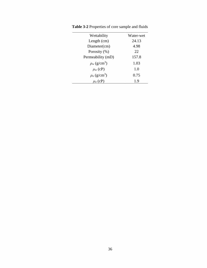
36
Table 3-2 Properties of core sample and fluids
Wettability Water-wet
Length (cm) 24.13
Diameter(cm) 4.98
Porosity (%) 22
Permeability (mD) 157.8
ρw (g/cm3) 1.03
μw (cP) 1.0
ρo (g/cm3) 0.75
μo (cP) 1.9

37
since the measured data are prepared every 60 minutes until the end of experiment (i.e.,
720 minutes). The measurement errors for cumulative water production, pressure drop,
and oil saturation are ±1 cm3, ±1 kPa, and ±0.01, respectively.
The true production data are generated as an output from the reservoir simulator
(CMG IMEX 2010.10) with the reference power-law model. Then, a Gaussian random
perturbation with the same standard deviation of the measurement errors is added to the
true data to generate the synthetic (reference) measurement data.
(1) Parameterization
In each model realization, the simulated variables include the cumulative water
production, pressure drop and oil saturation profile in every fifth grid (that is because the
oil saturation in every fifth grid is measured as observation data); the oil saturation in the
left grids and pressure in each grid are treated as dynamic variables; the static variables
are the parameters to define Equations [3-1]–[3-3], where there are total nine parameters,
aw, aow, *cowP , owce,P , nrw, nrow, ncow, Swi and Sorw. In general, in a drainage experiment, the
residual oil saturation, Sorw, is known as zero, while the end-point of water relative
permeability at the residual oil saturation can be fixed to be one. As such, the vector of
to-be-estimated parameters, i.e., the static variables, can be expressed as,
wiowce,*
cowcowrowrwows ,,,,,, SPPnnnam [3-18]
(2) Initialization
In order to use the ensemble-based history matching techniques to assimilate the
measurement data, the model-state should be initialized by generating an ensemble of Ne
38
initial model realizations, i.e., an ensemble of Ne sets of initial relative permeability and
capillary pressure curves, as reasonably as possible according to the prior knowledge. At
the beginning, a set of initial guess relative permeability and capillary pressure curves is
assigned according to prior knowledge. Combining the parameters to define the set of
initial guess relative permeability and capillary pressure curves, a vector of initial guess
static variables, i.e., an initial guess ms expressed by Equation [3-18], is obtained. Then,
Ne sets of Gaussian noise are added to the vector of initial guess static variables to
generate an ensemble of Ne vectors of initial static variables which are corresponding to
an ensemble of Ne sets of initial relative permeability and capillary pressure curves.
Since the error covariance in the ensemble-based method is estimated by using a finite
number of ensemble members, the ensemble size should be large enough to accurately
evaluate the error covariance, which is 200 (i.e., Ne = 200) in this study (Li, 2010; Li et
al., 2012).
3.2.2 Laboratory coreflooding experiment
The coreflooding experiment was conducted by Sun and Mohanty (2005), which was a
drainage process. A cylindrical water-wet Berea sandstone was used as the core sample
with the average absolute permeability of 157.8 mD and average porosity of 22%. The
length of the core is 24.13 cm and the diameter is 4.98 cm. The core was firstly saturated
with brine (15% NaCl) as the wetting phase, and then a mixture of Sotrol 130 and Iodl-
decane was used as the non-wetting phase to conduct the primary drainage experiment.
The core was put in a core holder which was vertically positioned on the table of a CT
scanner. The non-wetting phase was injected into the core from the top at a constant rate

39
of 0.375 cm3/min, while the fluid was produced at a constant outlet pressure of 1013 kPa.
During the experiment, the cumulative water production, pressure drop and oil saturation
profile were measured as the observation data to be assimilated, whose values can be
found elsewhere (Sun and Mohanty, 2005).
The numerical coreflooding experiment model described in Section 3.2.1 can be used
as the reservoir simulation model for the real coreflooding experiment due to the fact that
it is exactly setup according to this real coreflooding experiment. The variables in each
model realization of the real experiment are the same as those of the numerical
coreflooding experiment, which have been described in Section 3.2.1. The initial guess
static variables for the numerical coreflooding experiment are also set to be the initial
guess static variables for the real experiment, except that the initial guess Swi is assumed
to be 0.3. Then, the initialization method proposed in Section 3.2.1 is used to generate
the multiple initial models for the real experiment.
3.3 Results and Discussion
3.3.1 Numerical coreflooding experiment
In this section, the EnKF algorithm is validated by using the numerical coreflooding
experiment. The estimated results for the parameters together with their corresponding
reference values are tabulated in Table 3-3, where the mean and standard deviation
values obtained from the initial and updated ensembles are presented as well. All of the
parameters are found to approach their reference values through history matching, while
the corresponding standard deviations are reduced, indicating that uncertainties of the
parameters are greatly removed after the data assimilation process. It can also be seen

40
Table 3-3 Estimation results for numerical coreflooding experiment
Parameter Reference
value
Initial value Updated value
Mean Standard
deviation Mean
Standard
deviation
aow 0.850 0.804 0.080 0.854 0.012
nrw 4.000 2.500 1.000 3.970 0.011
nrow 2.500 3.500 1.000 2.470 0.016
ncow 6.000 3.500 1.000 5.826 0.170
*cowP 48.26 49.02 1.000 48.16 0.589
owce,P 2.070 2.511 0.500 2.014 0.447
Swi 0.180 0.101 0.100 0.171 0.001

41
that both *
cowP and owce,P are not estimated as accurately as the other parameters.
The updating process of the parameters is depicted in Figure 3-2. Significant
uncertainty is found to be associated with the parameters at early stage of the
assimilation process, though it is generally reduced as time proceeds. Eventually, the
updated parameters approach their corresponding reference values, while the variances
are reduced significantly except for *
cowP and owce,P . The estimated nrw and nrow are more
accurate than ncow, while better estimation results of nrw and nrow can be obtained with
relative less data assimilation times compared with ncow. In addition, variances of nrw and
nrow are reduced more quickly than that of ncow. This is because the relative permeability
curves are more sensitive to the measurement data. It can also be found that the
estimated *
cowP and owce,P still have larger uncertainty ranges, though the updated values
are approaching to their reference values. This may be resulted from their less sensitivity
to the measurement data. As such, good initial guesses should be either assigned to *
cowP
and owce,P according to the prior knowledge.
The reference, initial guess and updated relative permeability and capillary pressure
curves are plotted in Figure 3-3. The reference relative permeability and capillary
pressure curves are generated from the reference power-law model represented by
Equations [3-15]–[3-17], while the initial relative permeability and capillary pressure
curves are assigned according to prior knowledge. The updated curves are made
available from the updated power-law model whose parameters are the mean values of
the updated ensemble members. Although there is a large deviation between the initial
and reference relative permeability and capillary pressure curves, there is an excellent
agreement between the updated and reference curves by assimilating all of observed data.
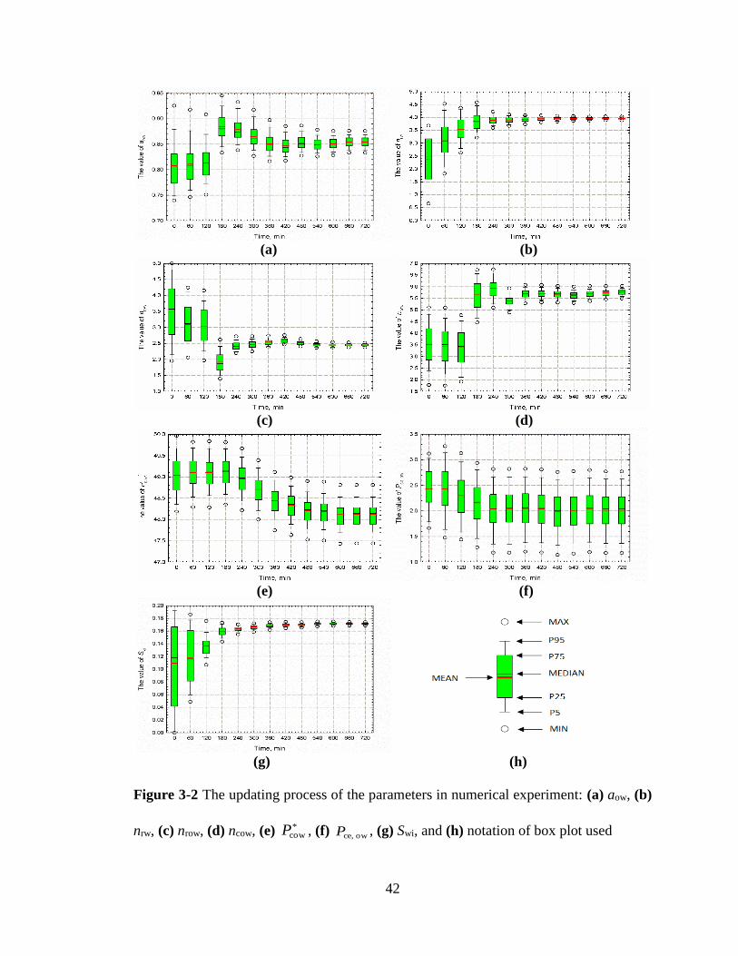
42
(a) (b)
(c) (d)
(e) (f)
(g) (h)
Figure 3-2 The updating process of the parameters in numerical experiment: (a) aow, (b)
nrw, (c) nrow, (d) ncow, (e) *cowP , (f) owce,P , (g) Swi, and (h) notation of box plot used

43
(a)
(b)
Figure 3-3 The reference, initial guess and updated average (a) Relative permeability
curves and (b) Capillary pressure curves for numerical experiment

44
The history matching results of the cumulative water production and pressure drop are
illustrated in Figure 3-4, respectively. There is a large deviation between the initial and
reference production history profiles due to the large deviation between the initial and
reference relative permeability and capillary pressure curves. Especially, water
breakthrough time of the initial case is around 165 minutes, which occurs later than that
(i.e., around 135 minutes) of the reference and updated cases, respectively. It can also be
seen from Figure 3-4 that cumulative water production history of the reference, initial
and updated cases are overlapped at the early stage since it is a piston-like displacement
process prior to water breakthrough.
The comparison between the reference, initial and updated in-situ oil saturation
profiles is plotted in Figure 3-5. There also exists an excellently matched saturation
profiles. Through this numerical coreflooding experiment, it has proven that the relative
permeability and capillary pressure curves can be simultaneously determined accurately
by using the EnKF algorithm to history match the coreflooding experiment.
3.3.2 Laboratory coreflooding experiment
The determined relative permeability and capillary pressure curves by using the
developed confirming EnKF technique are shown in Figure 3-6, while the estimated
relative permeability and capillary pressure by Sun and Mohanty (2005) are shown in
Figure 3-7. The differences between these estimation results may be attributed to the fact
that different estimation techniques and simulators have been used in these two studies.
In addition, the irreducible water saturation is estimated to be 0.25 by using the EnKF
algorithm, which is a little higher than the in-situ saturation value, i.e., 0.18, measured by

45
(a)
(b)
Figure 3-4 History matching results of (a) Cumulative water production and (b) Pressure
drop for numerical coreflooding experiment
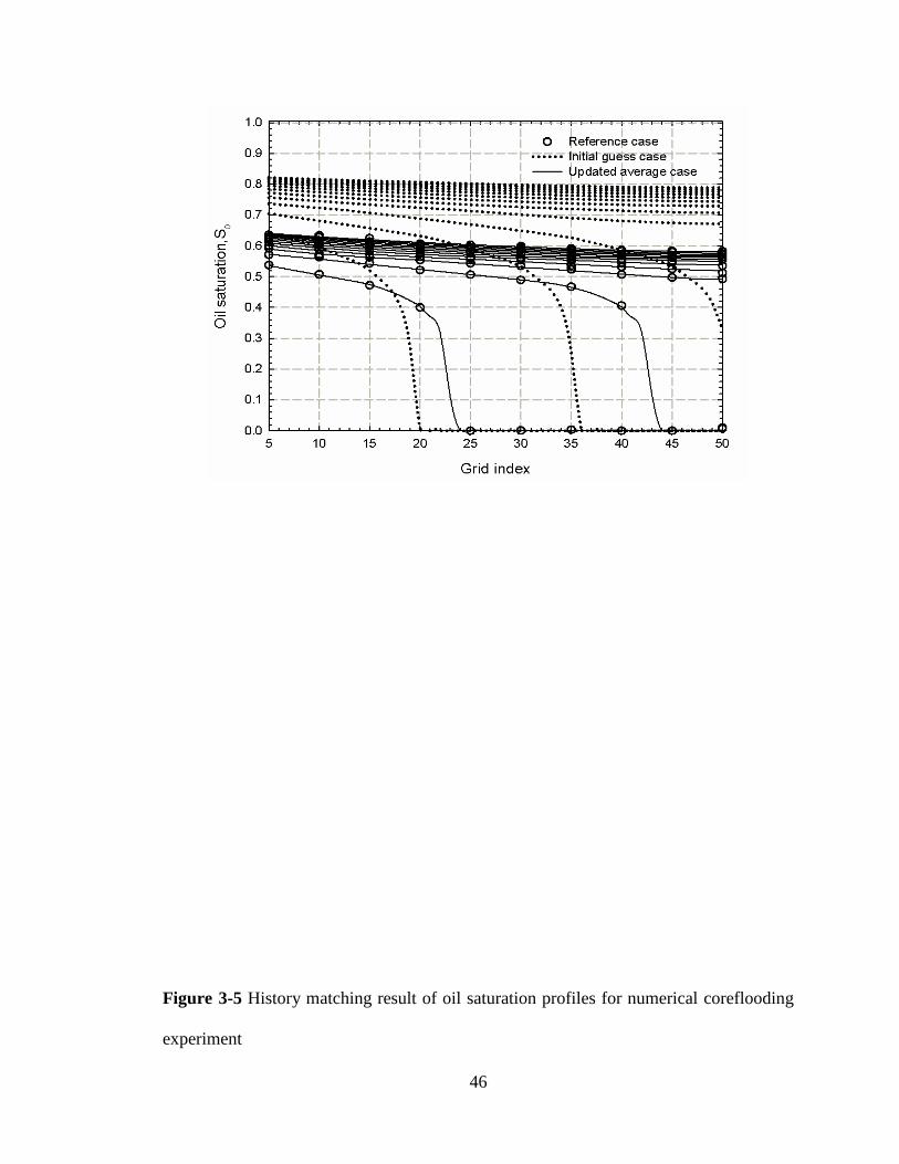
46
Figure 3-5 History matching result of oil saturation profiles for numerical coreflooding
experiment

47
Figure 3-6 Estimated relative permeability and capillary pressure curves for laboratory
coreflooding experiment by confirming EnKF technique

48
Figure 3-7 Estimated relative permeability and capillary pressure curves for laboratory
coreflooding experiment by Sun and Mohanty (2005)

49
using the CT scanning technique (Sun and Mohanty, 2005). As indicated by Sun and
Mohanty (2005), the irreducible water saturation measured by CT scanning maybe a
litter lower than the typical values due to the wettability variation in the inlet surface of
the core sample.
Figure 3-8 and Figure 3-9 show the history matching results of the confirming EnKF
technique, while Figure 3-10 and Figure 3-11 show the history matching results of Sun
and Mohanty (2005). As can be seen, in these two studies, similar good history matching
results are obtained for the pressure drop and cumulative water production, though minor
mismatches exist for the oil saturation profile. This is because, in addition to the
measurement error of the CT scans as mentioned by Sun and Mohanty (2005), different
reservoir simulators may not produce exact the same results. Another reason is that the
power-law model is used to represent the relative permeability and capillary pressure
curves in this section, while Sun and Mohanty (2005) used the B-spline model to
represent the relative permeability curves. As pointed out by Siddiqui et al. (1999) and
Kerig and Watson (1986), the simple functional form, such as the power-law model, may
result in some deviation between the simulated data and the experimental data.
3.4 Summary
An assisted history matching technique based on the EnKF algorithm has been
developed and successfully applied to simultaneously estimate relative permeability and
capillary pressure by assimilating coreflooding experiment data including cumulative
water production, pressure drop and oil saturation profiles in conventional reservoirs.
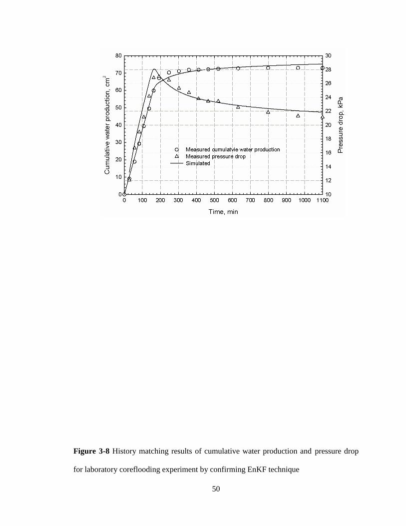
50
Figure 3-8 History matching results of cumulative water production and pressure drop
for laboratory coreflooding experiment by confirming EnKF technique

51
Figure 3-9 History matching result of oil saturation profiles for laboratory coreflooding
experiment by confirming EnKF technique

52
Figure 3-10 History matching results of cumulative water production and pressure drop
for laboratory coreflooding experiment by Sun and Mohanty (2005)

53
Figure 3-11 History matching result of oil saturation profiles for laboratory coreflooding
experiment by Sun and Mohanty (2005)

54
The power-law model has been employed to represent the relative permeability and
capillary pressure curves.
The newly developed technique is validated by using a numerical coreflooding
experiment. It has been found that the estimated relative permeability and capillary
pressure curves are improved and their uncertainty is reduced gradually as more
measurement data is assimilated. Finally, an excellent agreement between the updated
and reference relative permeability and capillary pressure curves has been obtained by
assimilating all of the measurement data, while good history matching has been made
available between the updated and reference production history profiles. It also found the
coefficients of the capillary pressure curve, especially the endpoints of *cowP and owce,P ,
are not estimated as accurately as the other parameters resulting from the fact that
capillary pressure is less sensitive to the measurement than the relative permeability.
As for the laboratory coreflooding experiment, the relative permeability and capillary
pressure curves are finally determined by assimilating all of the measurement data.
Although there is a minor mismatch for the oil saturation profiles, there exists a good
agreement between the measured and simulated pressure drop and cumulative water
production. The newly developed technique is easy to be implemented and well-suited
for uncertainty analysis under consistent framework.
55
CHAPTER 4 ESTIMATION OF RELATIVE PERMEABILITY
AND CAPILLARY PRESSURE FROM
DISPLACEMENT EXPERIMENTS WITH ENKF
TECHNIQUE IN TIGHT FORMATIONS
In this chapter, the EnKF algorithm is applied to simultaneously estimate relative
permeability and capillary pressure curves by history matching coreflooding experiment
data in a tight formation (Zhang et al., 2012c; Zhang and Yang, 2013a). The power-law
model and B-spline model have been employed to represent the relative permeability and
capillary pressure curves, respectively.
4.1 Methodology
As mentioned previously, the estimation of relative permeability and capillary pressure
can be reduced to a parameter estimation problem by using a suitable representation
model. The power-law model has been introduced in Section 3.1.1. The alternative
model is based on B-spline approximation of relative permeability and capillary pressure
curves. The B-spline model is very flexible and allows for the adjustment of different
parts of the aforementioned curves independently. The B-spline representation of relative
permeability and capillary pressure curves for oil-water flow is given by (Chen et al.,
2008),
1
3
wDrw
2wrw )()(n
j
jj SBCSk [4-1]
1
3
wDrow
2wrow )()(n
j
jj SBCSk [4-2]
56
1
3
wD
cow
2wcow )()(n
j
jj SBCSP [4-3]
where n is the number of segments divided on the curves, thus, there are n+1 control
knots on each curve. rwjC ,
row
jC and cow
jC are used to respectively denote the control
knots for the B-spline approximation of the water relative permeability, oil relative
permeability and capillary pressure curves. Bj is the base function for the B-spline
interpolation, which is a cubic polynomial for calculating the interpolation point value.
It should be noted that the B-spline curve passes through only two of its control knots,
the one labeled with subscript zero (i.e., the first control knot) and the one labeled with
subscript n (i.e., the last control knot). The B-spline curve is ‘attached’ to the other
control knots but does not normally pass through them. For each curve, there are two
control knots which are not shown, defined by (Li et al., 2010),
vvv CCC 101 2 , and v
n
v
n
v
n CCC 11 2 v = rw, row and cow [4-4]
Such a definition ensures that the B-spline curve will always pass through vC0 and
v
nC .
During the data assimilation process, model parameters are to be tuned randomly so
that the monotonicity of the relative permeability and capillary pressure curves cannot be
guaranteed if the control knots are used as the model parameters to be directly adjusted
in the optimization process (Li et al., 2012). As such, the reservoir simulation may be
unexpectedly terminated due to the fact that the reservoir simulator requires the relative
permeability and capillary pressure curves to be monotonic.
Two methods can be used to deal with this problem. As suggested by Chen et al.
(2008), the first method is that boundary conditions can be added to the control knots,
forcing the relative permeability and capillary pressure curves to be not only monotonic

57
but also concave up (Sun and Mohanty, 2005; Li and Horne, 2006). A curve is convex if
its derivative is a monotonically increasing function of dimensionless water saturation.
The convexity condition is given by,
v
j
v
j
v
j CCC 212 , for j = 1, 2,…, n, and )(2
111
v
j
v
j
v
j CCC , for j = 1, 2,…, n, [4-5]
However, this method reduces the flexibility of the B-spline representation due to the
imposed convexity condition.
The other method is to use the transformation suggested by Eydinov et al. (2009). For
a control knot,v
jC , on a relative permeability or capillary pressure curve, using its
neighbor knots, v
jC 1 and v
jC 1 , as its lower and upper bounds. Then the following
logarithm transformation is applied to the control knots vector,
njCC
CCx
v
j
v
j
v
j
v
jv
j
0,ln
1
1 [4-6]
where v
jx is the vector of pseudo-control knots, corresponding to the vector of control
knots on the relative permeability and capillary pressure curves (i.e.,v
jC ).
These new parameters, i.e.,v
jx , are to be tuned in the data assimilation process when
assimilating the measurement data sequentially. After assimilating each set of new
measurement data, the updated pseudo-control knots are obtained. In practice, the
pseudo-control knots do not have physical meaning and cannot be used as reservoir
parameters directly in the reservoir simulator. Therefore, the updated control knots
which are used to interpolate the updated relative permeability and capillary pressure
curves have to be inversely calculated from their corresponding updated pseudo-control
knots according to Equation [4-6]. The system of equations provided by Equation [4-6]

58
defines an one-to-one relationship between vjC and
vjx . The inverse transformation will
be defined by a linear system with n unknowns and n equations, where the matrix is
irreducibly diagonal dominant, and hence nonsingular. The solution of such a linear
system generates a unique vector of control knots, satisfying the condition of
monotonicity of the parameters, i.e., vjC , to ensure that the updated relative permeability
and capillary pressure curves are always monotonic.
In this chapter, the assisted history matching technique based on the EnKF algorithm
developed in CHAPTER 3 is used to simultaneously estimate relative permeability and
capillary pressure curves in a tight formation. The EnKF algorithm is firstly applied to
simultaneously estimate relative permeability and capillary pressure in the tight
formation by assimilating coreflooding experiment data including cumulative oil
production, pressure drop and water saturation profiles. It has been validated by using
the numerical coreflooding experiment where both power-law model and B-spline mode
are used to represent the relative permeability and capillary pressure curves. Then, the
EnKF algorithm is applied to simultaneously estimate relative permeability and capillary
pressure by assimilating coreflooding experiment data only including cumulative oil
production and pressure drop. Meanwhile, it has been validated by using a numerical
coreflooding experiment and then extended to a laboratory coreflooding experiment
where the power-law model is employed to represent the relative permeability and
capillary pressure curves.

59
4.2 Estimation with Saturation Profile
In this section, the EnKF algorithm is applied to simultaneously estimate relative
permeability and capillary pressure by history matching measurement data including
cumulative oil production, pressure drop and water saturation profile. The power-law
and B-spline models are respectively used to represent the relative permeability and
capillary pressure curves.
The numerical experiment is setup to simulate a coreflooding experiment (water
displacing oil) with a tight water-wet and heterogeneous core sample. The heterogeneous
core is placed horizontally and initially filled with oil and irreducible water. Then water
is injected at one end of the sample at a constant flow rate, while fluid is produced from
the other end at a constant pressure. The density and viscosity of the oil are 0.811 g/cm3
and 1.5 cP, respectively, while the density and viscosity of the water are 1.030 g/cm3 and
1.0 cP. The core sample model is divided into 50 × 1 × 1 grid blocks, all of which are
uniform with a dimension of 0.480 cm × 4.100 cm × 4.100 cm. The reference (true)
average absolute permeability is 0.5 mD with the standard deviation of 0.05, and its
upper boundary and lower boundary are 0.8 mD and 0.3 mD, respectively. The reference
relative permeability and capillary pressure curves are generated from the following
reference power-law model in which the reference values for both irreducible water
saturation (Swi) and residual oil saturation (Sorw) are set to be 0.36 and 0.40, respectively
(Kamath et al., 2001; Qin, 2002; Wang and Gu, 2011; Iwere et al., 2012),
5.3
wDwrw 35.0 SSk [4-7]
0.2
wDwrow 1 SSk [4-8]
05.310129.22685.3
wDwcow SSP [4-9]

60
In the experiment, the water is injected at a constant rate of 0.05 cm3/min, while the
fluid is produced at a constant outlet pressure of 1013 kPa. The measured data used for
assimilation include cumulative oil production, pressure drop and water saturation
profile. A total of 24 data points are available for assimilation since the measured data
are prepared every 30 minutes until the end of experiment (i.e., 720 minutes). The
measurement errors for cumulative oil production, pressure drop, and water saturation
are ±0.1 cm3, ±10 kPa, and ±0.01, respectively. The true production data are generated as
an output from the reservoir simulator (CMG IMEX 2010.10) with the reference power-
law model. Then, a Gaussian random perturbation with the same standard deviation of
the measurement errors is added to the true data to generate the synthetic measurement
data.
(1) Parameterization
In each model realization, the dynamic variables are pressure in each grid, while the
simulated variables are the corresponding synthetic measurement data which need to be
matched, including cumulative oil production, pressure drop, and water saturation profile.
According to different kinds of to-be-estimated parameters (i.e., static variables), two
scenarios are designed and compared in this study, i.e., power-law model and B-Spline
model are respectively used to represent the relative permeability and capillary pressure
curves.
As for Scenario #1, power-law model, i.e., Equations [3-1]–[3-3], is used to match the
synthetic measurement data. The relative permeability can be defined by normalizing
effective permeability using effective oil permeability at irreducible water saturation,
61
where absolute permeability is defined as k = ko(Swi). Thus, oil relative permeability must
be equal to unity when water saturation is equal to irreducible water saturation, i.e., aow =
1. In addition, the entry capillary pressure, owce,P , is assumed to be known since it can
usually be determined accurately according to the prior knowledge. As such, the vector
of to-be-estimated parameters in Scenario #1 is given by,
orwwi*
cowcowrowrwws ,,,,,, SSPnnnam [4-10]
As for Scenario #2, B-spline model, i.e., Equations [4-1]–[4-3], is used to match the
synthetic measurement data, while the static variables are the real-control knots on
relative permeability and capillary pressure curves. Since relative permeability is
normalized by ko(Swi), it leads to row
0C = 1. Oil relative permeability is zero at residual oil
saturation, i.e., row
nC = 0. As such, these two control knots will not be the model
parameters to be estimated. Then, there are n−1 to-be-estimated parameters for oil
relative permeability. Since water relative permeability is equal to zero at irreducible
water saturation, i.e., rw
0C = 0, there are n to-be-estimated parameters for water relative
permeability. In addition, there are n to-be-estimated parameters for capillary pressure
curve since the entry capillary pressure, i.e., cow
nC = owce,P , assumes to be known. Finally,
adding Swi and Sorw, there are total 3n+1 to-be-estimated parameters, whose vector can be
expressed as,
orwwicown
cow2
cow1
rwn
rw2
rw1
row1n
row2
row1s ,,,...,,,,...,,,,...,, SSCCCCCCCCC m [4-11]
The constraints defined by Equation [4-5] are applied to ensure that monotonic
relative permeability and capillary pressure curves are always obtained, while the

62
relative permeability and capillary pressure curves are divided into six segments (i.e., n =
6) uniformly in this section.
(2) Initialization
The initialization process of the power-law model has been described in Section 3.2.1.
As for the B-spline model, similar to the power-law model, a set of initial guess relative
permeability and capillary pressure curves can be assigned according to prior knowledge.
Combing the real-control knots on the set of initial guess relative permeability and
capillary pressure curves, Swi and Sorw, a vector of initial guess static variables, i.e., an
initial guess ms shown by Equation [4-11], is obtained. Then, the real-control knots in the
initial guess ms will be transformed into their corresponding pseudo-control knots
according to Equation [4-6], generating an initial guess pseudo-vector, msp,
orwwicown
cow2
cow1
rwn
rw2
rw1
row1n
row2
row1sp ,,,...,,,,...,,,,...,, SSxxxxxxxxx m [4-12]
Subsequently, various sets of Gaussian noise can be added to the initial guess pseudo-
vector to generate an ensemble of Ne initial pseudo-vectors. Finally, the pseudo-control
knots in the ensemble of Ne initial pseudo-vectors can be reversely transformed to obtain
their corresponding real-control knots generating an ensemble of Ne vectors of static
variables, which are corresponding to an ensemble of Ne sets of initial relative
permeability and capillary pressure curves. An ensemble size of 200 (i.e., Ne = 200) is
used in this section due to its small-scale application.
4.3 Estimation without Saturation Profile
Previous studies have proven that the EnKF algorithm can be used to simultaneously
estimate relative permeability and capillary pressure accurately in conventional

63
reservoirs and tight formations by assimilating displacement experiment data including
cumulative production data, pressure drop, and saturation profile (Zhang et al., 2012b;
Zhang and Yang, 2013a). Although fluid saturation profile is desirable for such
estimation, it is difficult to perform routine measurement for the fluid saturation profile
in the laboratory. This section is to examine the estimation accuracy of the EnKF
algorithm to simultaneously estimate relative permeability and capillary pressure by
assimilating conventional displacement experiment data only including cumulative oil
production and pressure drop. It is first demonstrated by using a numerical coreflooding
experiment and then extended to a laboratory coreflooding experiment. The power-law
model is used to represent the relative permeability and capillary pressure curves.
4.3.1 Numerical coreflooding experiment
The numerical experiment model and operation conditions designed in Section 4.2 are
also used in this subsection, except that the reference relative permeability and capillary
pressure curves are generated from the following reference power-law model in which
the reference values for both Swi and Sorw are also set to be 0.36 and 0.40, respectively,
5.3
wDwrw 35.0 SSk [4-13]
0.2
wDwrow 1 SSk [4-14]
56.123199.3718.2
wDwcow SSP [4-15]
The measured data used for assimilation only include cumulative oil production and
pressure drop, while a total of 18 data points are available for assimilation since the
measurement data are prepared every 30 minutes until the end of experiment (i.e., 540
minutes). The measurement errors for cumulative oil production and pressure drop are
64
±0.1 cm3 and ±10 kPa, respectively. The synthetic measurement data is generated in the
same way as that in Section 4.2. In each model realization, the dynamic variables include
grid pressure and water saturation of each grid, while the simulated variables are the
cumulative oil production and pressure drop. The power-law model is used to represent
the relative permeability and capillary pressure curves, so the static variables are the
coefficients of the power-law model.
As mentioned previously, there are total nine parameters, aw, aow, *
cowP , owce,P , nrw, nrow,
ncow, Swi and Sorw to define the power-law model. Previous studies have shown that it is
difficult to simultaneously estimate all of the coefficients by using the EnKF algorithm
to assimilate measurement data including cumulative production data, pressure drop and
saturation profile, especially for the endpoint values, such as *
cowP and owce,P . It will be
even more difficult for the EnKF algorithm to simultaneously estimate all of them by
assimilating the conventional measurement data which only include cumulative oil
production and pressure drop. Therefore, some parameters need to be pre-determined
according to prior knowledge. For example, oil relative permeability can be fixed to be
one at the irreducible water saturation (i.e., aow = 1). *
cowP and owce,P can be pre-determined
by using the J-Function according to prior knowledge. In addition, Swi and Sorw can be
fixed to be the values calculated directly from the coreflooding experiment, assuming
that the saturation is distributed uniformly. As such, the vector of to-be-estimated
parameters is expressed by,
cowrowrwws ,,, nnnam [4-16]
while its initialization process has been described in Section 3.2.1.

65
4.3.2 Laboratory coreflooding experiment
In this section, the EnKF algorithm is applied to a laboratory coreflooding experiment
(Zhang et al., 2012c). The oil and core samples used in this study are collected from a
tight formation with reservoir pressure of 11.5 MPa and temperature of 63°C in the
Bakken formation, Saskatchewan, Canada. The core sample is found to be water-wet
with dimension of 6.44 cm long and 3.81 cm in diameter. The density and viscosity of
the oil sample are measured to be 0.801 g/cm3 and 2.17 cP at atmospheric pressure and T
= 20°C, respectively. The synthetic brine is prepared and used in this study according to
the composition of the formation water. The density and viscosity of the formation water
are 1.11 g/cm3 and 1.24 cP at atmospheric pressure and T = 20°C, respectively.
(1) Experimental setup
The schematic diagram of the coreflooding apparatus used in this study is depicted in
Figure 4-1. A syringe pump is used to displace the crude oil and synthetic brine through
the core sample sealed in the coreholder, while both crude oil and synthetic brine are
stored in two high-pressure transfer cylinders, respectively. A high-pressure nitrogen
cylinder is connected with the coreholder to apply the so-called overburden pressure
which is always kept 3.0 MPa higher than the inlet pressure of the coreholder. A back-
pressure regulator (BPR) which is connected with another high-pressure nitrogen
cylinder is used to maintain the prespecified pressure in the coreholder during the
coreflooding experiment. The two high-pressure transfer cylinders and the coreholder are
placed inside an air-bath. An electric heater is used to heat the air-bath, and a
temperature controller is used to keep the air-bath at a constant temperature of 63±0.1°C
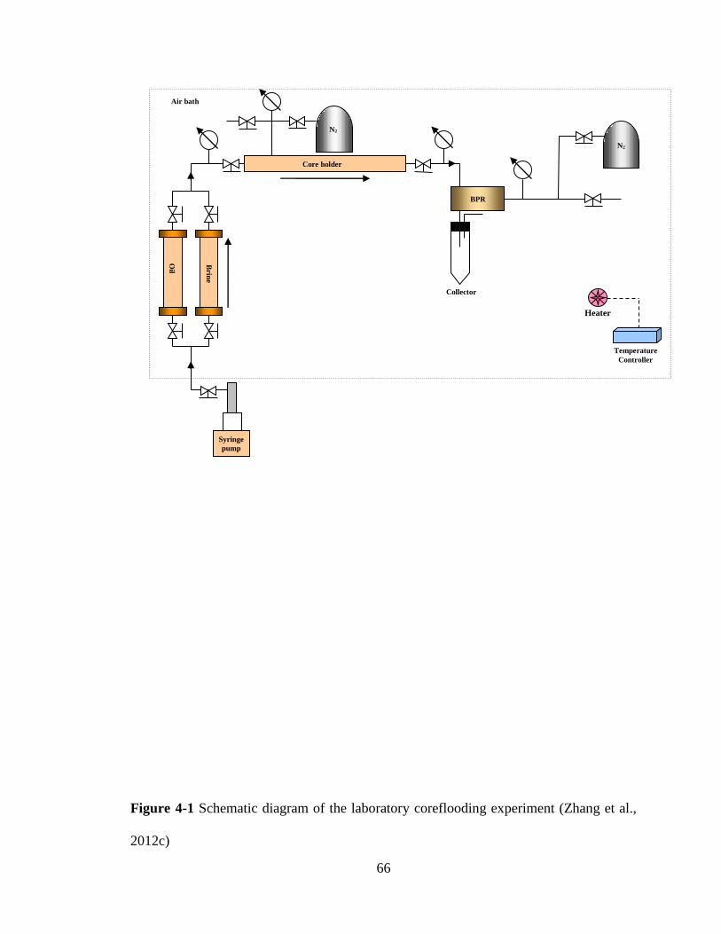
66
Figure 4-1 Schematic diagram of the laboratory coreflooding experiment (Zhang et al.,
2012c)
Core holder
N2
N2
BPR
Collector
Oil
Brin
e
Heater
Air bath
Syringe
pump
Temperature
Controller

67
during the coreflooding experiment. Pressure gauges are used to measure the inlet and
outlet pressures of the coreholder, respectively, while the overburden pressure and back
pressure are closely monitored by using pressure gauges. The produced oil is collected
and measured in a graduated sample collector.
(2) Experimental procedure
The general procedure for the coreflooding experiment is briefly described as follows
(Zhang et al., 2012c). The core sample is firstly cleaned with toluene, methanol, and
chloroform in sequence to remove the hydrocarbons, salts and clays in the core,
respectively. After the core sample is cleaned and dried, it is placed in the horizontal
coreholder and vacuumed for 12 hours. Then the synthetic brine is injected into the
cleaned core sample to measure its porosity according to mass balance. Sequentially, the
synthetic brine is injected into the core sample at different injection rates to measure its
absolute permeability according to Darcy’s law. The measured porosity and absolute
permeability of the core sample are 19.85% and 0.21 mD, respectively.
After measuring its porosity and absolute permeability, the water-saturated core
sample is flooded with crude oil until no water is produced. The irreducible water
saturation is determined on the basis of mass balance. After the core sample is fully
saturated with the crude oil, the core sample is further pressurized to the reservoir
pressure (i.e., 11.5 MPa). Then, the synthetic brine is injected at a constant injection rate
of 0.1 cm3/min and temperature of 63°C to recover the crude oil from the core sample
until no more oil is produced.
68
The residual oil saturation is also determined on the basis of mass balance. The
pressures at the inlet and outlet of the coreholder are respectively measured every 20
minutes with pressure gauges, which are used to determine the pressure drop across the
core sample. When the produced oil flows into the graduated sample collector, a
computer camera is used to record the volume of the produced oil, and the cumulative oil
production is determined every 20 minutes. The measurement errors of cumulative oil
production and pressure drop are ±0.1 cm3 and ±100 kPa, respectively.
(3) Numerical simulation
A two-phase (water and oil) black-oil simulator (i.e., CMG IMEX, version 2010.10) is
used to simulate the laboratory coreflooding experiment. The reservoir model is assumed
to be heterogeneous, whose average absolute permeability is determined to be 0.21 mD
with the standard deviation of 0.03. The reservoir model is equally divided into 50
blocks in the axial direction, each of which has a dimension of 0.13 cm. The simulated
measurement data include cumulative oil production and pressure drop.
The to-be-estimated parameters are the same as those of the numerical coreflooding
experiment as shown in Equation [4-16]. In the laboratory experiment, irreducible water
saturation, Swi, and residual oil saturation, Sorw, are determined on the basis of mass
balance of the experiment data. The *
cowP and owce,P are scaled by using the J-Function,
whose values are determined to be 547.17 kPa and 281.42 kPa, respectively. The
reference power-law model, i.e., Equations [4-13]–[4-15], where the values of *
cowP and
owce,P are changed accordingly to 547.17 kPa and 281.42 kPa, are used to generate the set
of initial guess relative permeability and capillary pressure curves for the laboratory
69
experiment. Then, model-state is initialized according to the initialization procedure
mentioned in Section 3.2.1.
4.4 Results and Discussion
4.4.1 Estimation with saturation profile
The reference power-law model, i.e., Equations [4-7]–[4-9], has been used for Scenarios
#1 and #2 to generate the synthetic measurement data. As for Scenario #1, coefficients of
the initial power-law model are updated by assimilating the synthetic measurement data
and finally compared with those of the reference power-law model. For Scenario #2, the
real-control knots used for interpolating the initial relative permeability and capillary
pressure curves are updated by assimilating the synthetic measurement data and finally
compared with those on the reference curves.
(1) Scenario #1
According to the initialization method described in Section 3.2.1, an ensemble of Ne sets
of relative permeability and capillary pressure curves are initialized as shown in Figure
4-2, where the reference curves are generated from the reference power-law model,
while the initial guess curves are generated from the initial guess power-law model
whose values are tabulated in Table 4-1. As can be seen from Figure 4-2, there exist
large uncertainty ranges for relative permeability and capillary pressure curves at
original time, respectively.
The coefficients of the power-law model are finally determined by assimilating all of
the synthetic measurement data with the estimation results listed in Table 4-1. As can be

70
Table 4-1 Estimation results for power-law model
Parameter Reference
value
Initial value
Updated value
Mean Standard
deviation Mean
Standard
deviation
aw 3.500×10⁻¹ 3.130×10⁻¹ 1.000×10⁻¹ 3.510×10⁻¹ 1.166×10⁻³
nrw 3.500×100 4.539×100 5.000×10⁻¹ 3.444×100 3.949×10⁻²
nrow 2.000×100 3.026×100 5.000×10⁻¹ 2.009×100 1.539×10⁻²
*cowP 2.268×10³ 2.510×10³ 1.000×10²
2.477×10³ 7.345×101
ncow 3.500×100 4.478×100 1.000×100
3.801×100 1.014×10⁻¹
Swi 3.600×10⁻¹ 2.730×10⁻¹ 1.000×10⁻¹ 3.610×10⁻¹ 2.232×10⁻³
Sorw 4.000×10⁻¹ 2.580×10⁻¹ 1.000×10⁻¹ 3.990×10⁻¹ 2.504×10⁻⁴

71
(a)
(b)
Figure 4-2 The reference and initial (a) Relative permeability curves and (b) Capillary
pressure curves in Scenario #1

72
seen, the mean values of the updated coefficients are closer to their corresponding
reference values compared to the initial ones. Also, standard deviations of the updated
coefficients are reduced dramatically throughout the history matching process, and thus
uncertainties of the coefficients have been greatly mitigated.
Figure 4-3 depicts variations of the to-be-estimated coefficients versus time.
Significant uncertainty is found to be associated with the coefficients at early stage,
though it is generally reduced as time proceeds. Eventually, the updated coefficients
approach their corresponding reference values, while the variances are reduced
significantly except for *
cowP . Although the coefficient of *
cowP is modified and approaches
to its reference value, its estimation result is not as accurate as the other coefficients with
a large uncertainty range even after updating. This may be resulted from its less
sensitivity to the measurement data, so *
cowP needs to be predetermined according to prior
knowledge.
The reference and updated average relative permeability and capillary pressure curves
are plotted in Figure 4-4, where the grey shadows are the ensemble of Ne updated relative
permeability and capillary pressure curves. The updated average curves are made
available from the updated average power-law model whose coefficients are the mean
values of the updated members. Obviously, there exists an excellent agreement between
the updated average and reference relative permeability and capillary pressure, while
their uncertainty ranges are reduced significantly compared with their initial cases as
shown in Figure 4-2.
The history matching results of cumulative oil production and pressure drop are
illustrated in Figure 4-5, respectively. There is a large deviation between the initial and

73
(a) (b)
(c) (d)
(e) (f)
(g)
Figure 4-3 Parameter (a) aw, (b) nrw, (c) nrow, (d) ncow, (e) *
cowP , (f) Swi and (g) Sorw of
power-law model as a function of assimilation time in Scenario #1
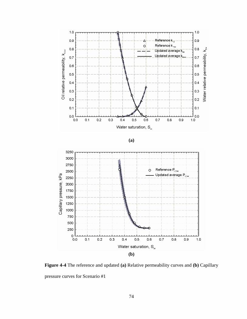
74
(a)
(b)
Figure 4-4 The reference and updated (a) Relative permeability curves and (b) Capillary
pressure curves for Scenario #1

75
(a)
(b)
Figure 4-5 History matching results of (a) Cumulative oil production and (b) Pressure
drop in Scenario #1
76
reference production history profiles due to the associated large uncertainties of the
initial model. Especially, water breakthrough time of the initial case is around 180
minutes, which occurs later than that of the reference and updated cases. It can also be
seen from Figure 4-5 that cumulative oil production history of the reference, initial and
updated cases are overlapped at the early stage since it is a piston-like displacement
process prior to water breakthrough. Figure 4-6 shows an excellent match for the
reference and updated in-situ water saturation profiles.
(2) Scenario #2
In this scenario, the B-spline model is used to match the synthetic measurement data.
The reference power-law model defined by Equations [4-7]–[4-9] is still used to generate
the reference relative permeability and capillary pressure curves. At time zero, a set of
initial guess relative permeability and capillary pressure curves is assumed according to
the prior knowledge (see Figure 4-7), where the black solid symbols on each curve are
the initial guess real-control knots to interpolate the corresponding curves. According to
the initialization process mentioned previously, an ensemble of Ne sets of initial relative
permeability and capillary pressure curves are generated (see Figure 4-7). Compared
with Figure 4-2 (i.e., Scenario #1), there are larger uncertainty ranges associated with the
initial relative permeability and capillary pressure curves in Scenario #2, which
demonstrates that the B-spline interpolation can represent the relative permeability and
capillary pressure curves more flexible than the power-law model.
Figure 4-8 shows the estimated average relative permeability and capillary pressure
curves for Scenario #2, where the grey shadows are the ensemble of Ne sets of updated

77
Figure 4-6 History matching result of water saturation profiles in Scenario #1

78
(a)
(b)
Figure 4-7 The reference and initial (a) Relative permeability curves and (b) Capillary
pressure curves for Scenario #2
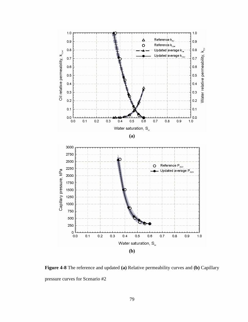
79
(a)
(b)
Figure 4-8 The reference and updated (a) Relative permeability curves and (b) Capillary
pressure curves for Scenario #2

80
relative permeability and capillary pressure curves. The black symbols on each curve are
the updated mean real-control knots to interpolate their corresponding updated average
curves, which are the mean values of the updated ensemble members. Obviously, the
updated mean real-control knots are all approaching their reference real-control knots
through history matching. It can also be seen from Figure 4-8 that there is an excellent
agreement between the updated average and reference relative permeability and capillary
pressure curves, and the uncertainty ranges of the updated relative permeability and
capillary pressure curves are significantly reduced compared with their initial cases. The
agreement, however, is not as good as that of Scenario #1 due to the fact that more
flexibility is introduced by using the B-spline interpolation model (Sun and Mohanty,
2005). The water relative permeability curves can be estimated slightly more accurately
than the oil relative permeability curves, indicating that the water relative permeability is
slightly more sensitive to the measurement data. This may mainly be due to the nature of
the water-wet rock used in this study. Similarly, it is found from centrifugal experiments
that the recovery calculations are more sensitive to changes in the parameters of the
wetting phase relative permeability compared to those of the non-wetting phase relative
permeability (Firoozabadi and Aziz, 1991).
The updating process of the to-be-estimated parameters (i.e., the real-control knots) in
this scenario is similar to Scenario #1. There is significant uncertainty associated with
the parameters at early stage of the assimilation process, while it is generally reduced as
time proceeds. Eventually, all of the to-be-estimated parameters approach their
corresponding reference values and their variances are reduced significantly as well.
Figure 4-9 presents several typical real-control knots, Swi and Sorw change versus time.
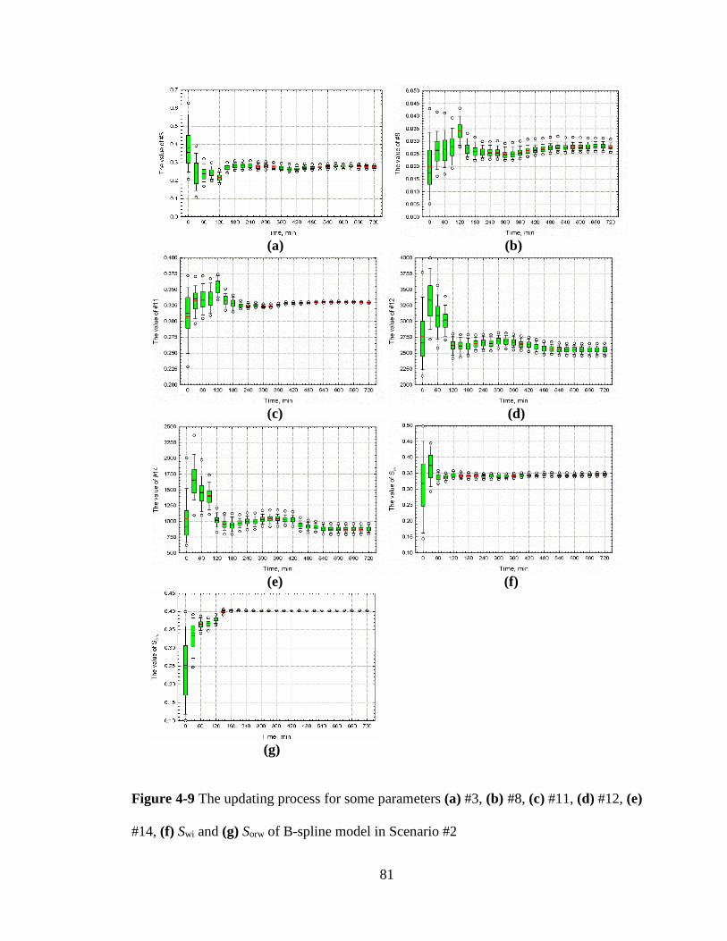
81
(a) (b)
(c) (d)
(e) (f)
(g)
Figure 4-9 The updating process for some parameters (a) #3, (b) #8, (c) #11, (d) #12, (e)
#14, (f) Swi and (g) Sorw of B-spline model in Scenario #2

82
The real-control knot #3 is on the oil relative permeability curve. The real-control knots
#8 and #11 are on the water relative permeability curve, among which knot #11 is the
endpoint of the water relative permeability curve, corresponding to aw in the power-law
model. The real-control knots #12 and # 14 are on the capillary pressure curve, among
which knot #12 is the endpoint of the capillary pressure curve, corresponding to *cowP in
the power-law model. It can be seen from Figure 4-9f and g that the estimated Sorw,
which is closer to its reference value and with a smaller variance, is more accurate than
that of Swi. This may be attributed to the fact that Sorw is more sensitive to the
measurement data. However, the endpoint of the capillary pressure curve, i.e., real-
control knot #12, is not estimated as accurately as the other parameters, which is also
consistent with the finding in Scenario #1.
The history matching results of cumulative oil production and pressure drop are
depicted in Figure 4-10. Compared with Scenario #1, a larger uncertainty associated with
the initial relative permeability and capillary pressure curves in Scenario #2 causes a
larger deviation between the initial and reference production history profiles. Obviously,
the water breakthrough time of the initial case which is around 250 minutes occurs later
than that (i.e., around 120 minutes) of the reference and updated cases. After assimilation,
there still exists an excellent agreement between the updated and reference cumulative
oil production history profile. However, there is a minor mismatch for the updated and
reference pressure drop due to the small deviation between the updated and reference
relative permeability and capillary pressure curves. The comparison between the
reference and updated in-situ water saturation profiles is plotted in Figure 4-11. The
saturation profiles are also matched excellently.

83
(a)
(b)
Figure 4-10 History matching results for (a) Cumulative oil production and (b) Pressure
drop in Scenario #2

84
Figure 4-11 History matching result for water saturation profiles in Scenario #2

85
4.4.2 Estimation without saturation profile
(1) Numerical coreflooding experiment
As for only assimilating the conventional measurement data, there is insufficient
information to estimate all of the coefficients of power-law model simultaneously and
accurately. The parameters Swi , Sorw, *
cowP and owce,P are assumed to be known, while only
aw and three shape factors (i.e., nrow, nrw and ncow) need to be estimated. The estimated
result is shown in Table 4-2, where the mean and standard deviation values obtained
from the initial and updated ensemble are presented. As can be seen, the mean values of
the updated coefficients are approaching much closer to the corresponding reference
values compared to the initial ones. Also, standard deviations of the updated coefficients
are reduced dramatically throughout the history matching process, and thus uncertainty
of the coefficients has been greatly reduced.
Figure 4-12 shows the to-be-estimated coefficients change versus time. Obviously,
uncertainty is significantly associated with the four coefficients at the early stage and
gradually improved as the time proceeds. Eventually, all of the four coefficients are
closely approaching their reference values, while the associated uncertainty is minimized.
The estimated aw, nrow and nrw are more accurate than ncow, while better estimation results
of aw, nrow and nrw can be obtained with relative less data assimilation times compared
with ncow. This can be explained by the fact that relative permeability is more sensitive to
the conventional measurement data, while capillary pressure imposes a dominant impact
on saturation distribution. The estimation accuracy of capillary pressure has been found
to significantly improve by assimilating additional measurement data (i.e., saturation
profile) (Watson et al., 1998; Sun and Mohanty, 2005; Li et al., 2010).
The reference, initial and updated relative permeability and capillary pressure curves

86
Table 4-2 Estimation results for numerical coreflooding experiment
Parameter Reference
value
Initial value Updated value
Mean Standard
deviation Mean
Standard
deviation
aw 0.350 0.249 0.052 0.346 0.001
nrow 2.000 1.445 0.438 1.995 0.006
nrw 3.500 1.451 0.483 3.485 0.036
ncow 2.800 1.305 0.456 2.628 0.155

87
(a) (b)
(c) (d)
Figure 4-12 (a) aw, (b) nrow, (c) nrw, and (d) ncow as a function of assimilation time for
the numerical coreflooding experiment
88
are plotted in Figure 4-13. The reference relative permeability and capillary pressure
curves are generated from the reference power-law models, while their initial values are
obtained from the initial guess power-law model. The updated curves are made available
from the updated power-law model whose coefficients are the mean values of the
updated ensemble members. Obviously, an excellent agreement is found not only
between the updated and reference relative permeability, but also between the updated
and reference capillary pressure. The history matching results are shown in Figure 4-14.
There exists an excellent agreement between the measured and updated production
profiles.
(2) Laboratory coreflooding experiment
Similar to the numerical coreflooding experiment, only the endpoint of water relative
permeability (i.e., aw) and three shape factors (i.e., nrow, nrw, ncow) are to be estimated,
because*
cowP , owce,P , Swi and Sorw have been determined according to the prior knowledge.
The finally determined relative permeability and capillary pressure curves are plotted in
Figure 4-15.
Figure 4-16 shows the history matching results between the data generated by the
determined relative permeability and capillary pressure curves and the experimental data.
As for the cumulative oil production (Figure 4-16a), there is an excellent match between
the measured and simulated data at the beginning stage (i.e., before water breakthrough),
then followed by an obvious mismatch, especially during the water breakthrough period.
The excellent match is ascribed to the fact that it is a piston-like displacement prior to
water breakthrough. The followed mismatch may be caused by the fact that, in addition
to the experimental errors, the nonlinearity of the whole data assimilation system is

89
(a)
(b)
Figure 4-13 The reference, initial and updated (a) Relative permeability curves and (b)
Capillary pressure curves for the numerical coreflooding experiment

90
(a)
(b)
Figure 4-14 History matching results of (a) Cumulative oil production and (b) Pressure
drop for the numerical coreflooding experiment

91
Figure 4-15 Estimated relative permeability and capillary pressure curves for the
laboratory coreflooding experiment

92
(a)
(b)
Figure 4-16 History matching results of (a) Cumulative oil production and (b) Pressure
drop for the laboratory coreflooding experiment

93
further enhanced without fluid saturation profile data, resulting in strongly nonlinear data
assimilation system where the EnKF algorithm may not function well. Another possible
reason for the mismatch is that, as pointed out by Kerig and Watson (1986) and Siddiqui
et al. (1999), the simple functional form, such as power-law model, may result in certain
deviation of the simulated data from its experimental values. As can be seen from Figure
4-16b, a reasonable good match is obtained for the pressure drop.
4.5 Summary
The newly developed assisted history matching technique based on the EnKF algorithm
has been applied to simultaneously estimate relative permeability and capillary pressure
curves in tight formations by history matching coreflooding experiment data. The new
technique is first applied to the situation where fluid saturation profile is available to be
assimilated, while it has been validated by using the numerical coreflooding experiment
where both power-law and B-spline models are used to represent the relative
permeability and capillary pressure curves. Subsequently, the new technique is applied to
the scenarios where fluid saturation profile is not available to be assimilated, while it has
been validated by using a numerical experiment and then extended to a laboratory
coreflooding experiment where power-law model is used as the representation model.
No matter whether the fluid saturation profile is available or not, the relative
permeability and capillary pressure curves are updated progressively and their
uncertainty is reduced gradually as more measurement data is assimilated in the
numerical coreflooding experiments. Accordingly, an excellent agreement between the
updated and reference relative permeability and capillary pressure curves has been

94
obtained by assimilating the available measurement data completely, while good history
matching has been made available between the updated and reference production history
profiles. In addition, the relative permeability is found to be estimated more accurately
than the capillary pressure owing to its more sensitivity to the measurement data.
Moreover, the B-spline model can be used to represent the relative permeability and
capillary pressure curves more flexible than the power-law model.
As for the laboratory coreflooding experiment, the relative permeability and capillary
pressure curves are finally determined by using the EnKF algorithm to assimilate all of
the measurement data. Although there is a reasonable good history matching for the
pressure drop, an obvious mismatch exists for the cumulative oil production. In addition
to the experiment error and the limitation of the power-law representation model, this
may be caused by the linear assumption in the updating step of the EnKF algorithm that
makes it not function well for the strongly nonlinear data assimilation system. Therefore,
it is desirable that the existing techniques need to be improved for the strongly nonlinear
data assimilation system.

95
CHAPTER 5 ESTIMATION OF RELATIVE PERMEABILITY
AND CAPILLARY PRESSURE FOR TIGHT
FORMATIONS BY ASSIMILATING FIELD
PRODUCTION DATA WITH ENKF TECHNIQUE
In this chapter, the newly developed history matching technique based on the EnKF
algorithm has been extended to simultaneously evaluate relative permeability and
capillary pressure for tight formations by history matching the field production data
(Zhang and Yang, 2013b). The power-law model is used to represent the relative
permeability and capillary pressure curves. The technique has been validated by using a
synthetic 2D reservoir model with two scenarios, where two-phase and three-phase
relative permeability together with capillary pressure curves are evaluated, respectively.
5.1 Methodology
The power-law model is used to represent the relative permeability and capillary
pressure curves in this study, which has been extensively used in field-scale reservoir
simulation owing to its simplicity. The power-law representation for the two-phase oil-
water relative permeability and capillary pressure curves has been defined in Section
3.1.1. Similarly, for the gas-oil system, the relative permeability and capillary pressure
curves can be respectively expressed as (Reynolds et al., 2004),
rg
gcwiorg
gcg
ggrg
1)(
n
SSS
SSaSk
[5-1]

96
rog
gcwiorg
gwiorg
oggrog
1
1)(
n
SSS
SSSaSk
[5-2]
ogce,
gcwiorg
gcg*coggcog
cog
1)( P
SSS
SSPSP
n
[5-3]
where krg is gas relative permeability, krog is oil relative permeability in the gas-oil
system, Sg is gas saturation, Sgc is the critical gas saturation, Sorg is the residual oil
saturation in the gas-oil system, ag is the endpoint of gas relative permeability curve, aog
is the endpoint of oil relative permeability curve in the gas-oil system. Pcog is gas-oil
capillary pressure, ogce,P is the entry capillary pressure for the gas-oil system,
(ogce,
*
cog PP ) is the capillary pressure at maximum gas saturation. The exponents, nrg, nrog
and ncog, establish the curvature, which are changed with the pore geometry
configuration (Blunt, 2001; Barrera, 2007).
In a three-phase flowing region, the water and gas relative permeability can still be
calculated by using Equations [3-1] and [5-1], respectively, while the oil-water and gas-
oil capillary pressures can also be determined from Equations [3-3] and [5-3],
respectively. However, the oil relative permeability at a particular water and gas
saturation, kro, is calculated by using the modified Stone II Model (Stone, 1973; Li et al.,
2012) as follows,
rgrwrg
og
rog
rw
ow
row
owro kkka
kk
a
kak [5-4]
Hence, for two-phase flow in porous media, parameters either in Equations [3-1]–[3-3]
for the oil-water flow or in Equations [5-1]–[5-3] for the gas-oil flow are to be estimated,
while, for the three-phase flow, parameters in these six equations need to be estimated.
97
In this chapter, the EnKF algorithm is still used to assimilate the production data,
while its detailed workflow has been described in Section 3.2. To overcome the problem
that the updated dynamic state variables and simulated variables may not be consistent
with the updated static variables caused by the nonlinearity, after each updating step, a
confirming component which is similar to the confirming EnKF technique has been
introduced into the workflow. In lieu of rerunning the simulator from previous
assimilation time to current assimilation time, the proposed procedure is to rerun the
simulator from time zero to the current assimilation time by using the updated static
variables for achieving the confirming purpose.
5.2 Synthetic Reservoir Model
5.2.1 Simulation model
A synthetic 2D heterogeneous reservoir model is used to validate the new technique. The
reservoir model contains 15×15×1 gridblock which is uniform with areal dimension of
10.20 m×10.20 m, and the thickness of the gridblock is 9.20 m. The depth of the
reservoir is 2340 m. The absolute permeability field and porosity field are generated by
using the geostatistical simulation technique constrained to the observed hard data at
each well location. The absolute permeability and porosity fields are shown in Figure 5-1.
The reservoir rock is water-wet, while the synthetic reservoir is under-saturated. The
initial reservoir pressure and water saturation are set to be 31,026 kPa and 0.26,
respectively. The densities of oil, gas and water are set to be 779.22 kg/m3, 1.12 kg/m3
and 1009.3 kg/m3, respectively. The reference relative permeability and capillary
pressure curves are generated by using the B-spline interpolation.
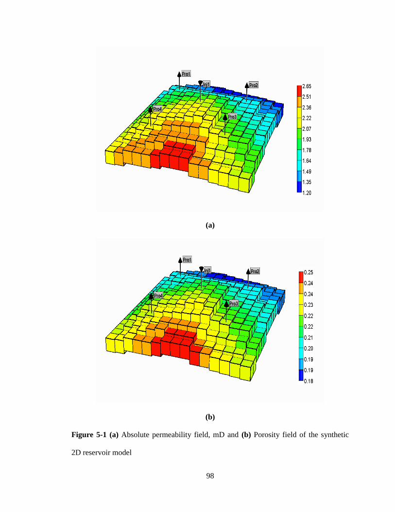
98
(a)
(b)
Figure 5-1 (a) Absolute permeability field, mD and (b) Porosity field of the synthetic
2D reservoir model

99
The synthetic reservoir model is a five-spot waterflooding pattern as shown in Figure
5-1. A water injection well (i.e., Inj1) is completed in gridblock (8, 8), where water is
injected at a constant rate of 71.54 m3/d all the time. Production wells are located in
gridblock (4, 4) for well Pro1, (12, 4) for well Pro2, (12, 12) for well Pro3, and (4, 12)
for well Pro4, respectively. Each of these wells is produced at a constant total fluid rate
of 15.90 m3/d. All the test scenarios presented in this chapter are based on this reference
model.
5.2.2 Test scenarios
(1) Two-phase flow
Two-phase oil-water relative permeability and capillary pressure curves are to be
estimated in this scenario since the reservoir pressure is always maintained above the
bubble-point pressure, resulting in only two-phase oil-water flow. There are total nine
parameters, aw, aow, *
cowP , owce,P , nrw, nrow, ncow, Swi and Sorw, to define Equations [3-1]–
[3-3]. As mentioned previously, the oil relative permeability at irreducible water
saturation can be normalized to be 1.0 (i.e., aow = 1.0), while the irreducible water
saturation (i.e., Swi) can be fixed since it can be determined accurately according to prior
knowledge. As for the two-phase oil-water flow considered here, it is an imbibition
process as the reservoir rock is water-wet. Thus, the entry capillary pressure for the oil-
water capillary pressure curve can be fixed to be zero (i.e., owce,P = 0). Since
*cowP is
previously found to be insensitive to the production data resulting in poor estimation
accuracy, it is also fixed in this study (Zhang et al., 2012b; Zhang and Yang, 2013a). In

100
practice, *
cowP can also be pre-determined according to prior knowledge. As such, the
vector of to-be-estimated parameters in this scenario can be expressed as,
orwcowrowrwws ,,,, Snnnam [5-5]
The production data used for assimilation include water-oil ratio and cumulative oil
production of each production well from the first 750 days of production. As the
production data are recorded every 30 days at each well, a total of 200 data points are
available for assimilating. The measurement errors for water-oil ratio and cumulative oil
production are ±0.1 and ±10 m3, respectively. The reference production data are
generated as an output from the reservoir simulator (CMG IMEX 2010.10) with the
reference model. Then, a Gaussian random perturbation with the same standard deviation
of the measurement errors is added to the reference data to generate the synthetic
observed production data.
(2) Three-phase flow
In this scenario, the reservoir pressure drops below the bubble-point pressure shortly
after the beginning of production so that gas will be released from the oil, resulting in
three-phase flow in the reservoir. As for the estimation of three-phase relative
permeability and capillary pressure curves, parameters used to define both oil-water and
gas-oil relative permeability and capillary pressure curves need to be estimated. As for
the oil-water system (i.e., Equations [3-1]–[3-3]), the to-be-estimated parameters are the
same as those in two-phase flow, which have been shown in Equation [5-5]. As for the
gas-oil system, in addition to Swi, there are nine parameters, ag, aog, *
cogP , ogce,P , nrg, nrog,
ncog, Sgc and Sorg. In practice, aog can be normalized to be one. Sgc equals zero since the
101
synthetic reservoir is under-saturated, but the procedure is universal and applicable to
cases where Sgc is not equal to zero, such as the existing gas cap or saturated reservoir.
There exists entry capillary pressure (i.e., ogce,P ) for the gas-oil capillary pressure curve
due to the fact that the gas-oil flow in the synthetic reservoir is a drainage process.
However, the end-points of the capillary pressure curve are previously found to be
insensitive to the production data (See CHAPTER 3 and CHAPTER 4), resulting in poor
estimation accuracy for them, so *cogP and
ogce,P are fixed in this study. In practice, they
can also be pre-determined according to prior knowledge. Finally, the vector of to-be-
estimated parameters can be expressed as,
orgcogrogrggorwcowrowrwws ,,,,,,,,, SnnnaSnnnam [5-6]
The production data used for assimilation include oil production rate, water
production rate, gas production rate and cumulative oil production of each well from the
first 600 days of production, which are recorded every 30 days. Then, a total of 320 data
points are available for assimilating. The measurement errors for the oil production rate,
water production rate, gas production rate and cumulative oil production are ±0.1 m3/d,
±0.1 m3/d, ±1 sm3/d and ±10 m3, respectively. The synthetic observed production data is
generated in the same way.
As mentioned previously, in order to use the ensemble-based history matching
technique to assimilate the production data, an ensemble of Ne sets of relative
permeability and capillary pressure curves should be initialized as accurately as possible
according to the prior knowledge. The initialization process of the power-law
representation has been described in Section 3.2.1 in detail.
102
5.3 Results and Discussion
5.3.1 Two-phase flow
In this scenario, two-phase oil-water relative permeability and capillary pressure curves
are estimated by assimilating water-oil ratio and cumulative oil production of each well.
According to the initialization method, an ensemble of Ne sets of initial relative
permeability and capillary pressure curves is generated as shown in Figure 5-2, where
there exist large uncertainty ranges for relative permeability and capillary pressure
curves at initial time, respectively.
Then, ensembles of initial water-oil ratio profiles and initial cumulative oil production
profiles for each well are respectively obtained by running the reservoir simulator with
the ensemble of Ne sets of initial relative permeability and capillary pressure curves,
which are respectively shown in Figure 5-3 − Figure 5-6. Obviously, there exist wide
uncertainty ranges for the ensembles of initial water-oil ratio profiles and initial
cumulative oil production profiles due to the large uncertainty in the initial relative
permeability and capillary pressure curves. Meanwhile, the reference water-oil ratio and
cumulative oil production are all respectively covered by the ensembles of initial water-
oil ratio profiles and initial cumulative oil production profiles.
The to-be-estimated parameters are finally determined by assimilating all of the
production data with the estimation results listed in Table 5-1, while the finally
determined values (i.e., the updated values) are the mean values of the updated ensemble
members. Obviously, standard deviations of the determined parameters are reduced

103
Table 5-1 Estimation results for two-phase flow
Parameter Initial value Updated value
Mean Standard
deviation Mean
Standard
deviation
aw 4.50×10⁻¹ 1.00×10⁻¹ 3.52×10⁻¹ 7.49×10⁻⁴
nrw 3.00×100 5.00×10⁻¹ 1.93×100 6.73×10⁻³
nrow 1.80×100 5.00×10⁻¹ 2.29×100 4.72×10⁻³
ncow 2.50×100 5.00×10⁻¹ 3.39×100 8.30×10⁻²
Sorw 2.00×10⁻¹ 1.00×10⁻¹ 3.09×10⁻¹ 3.38×10⁻⁴
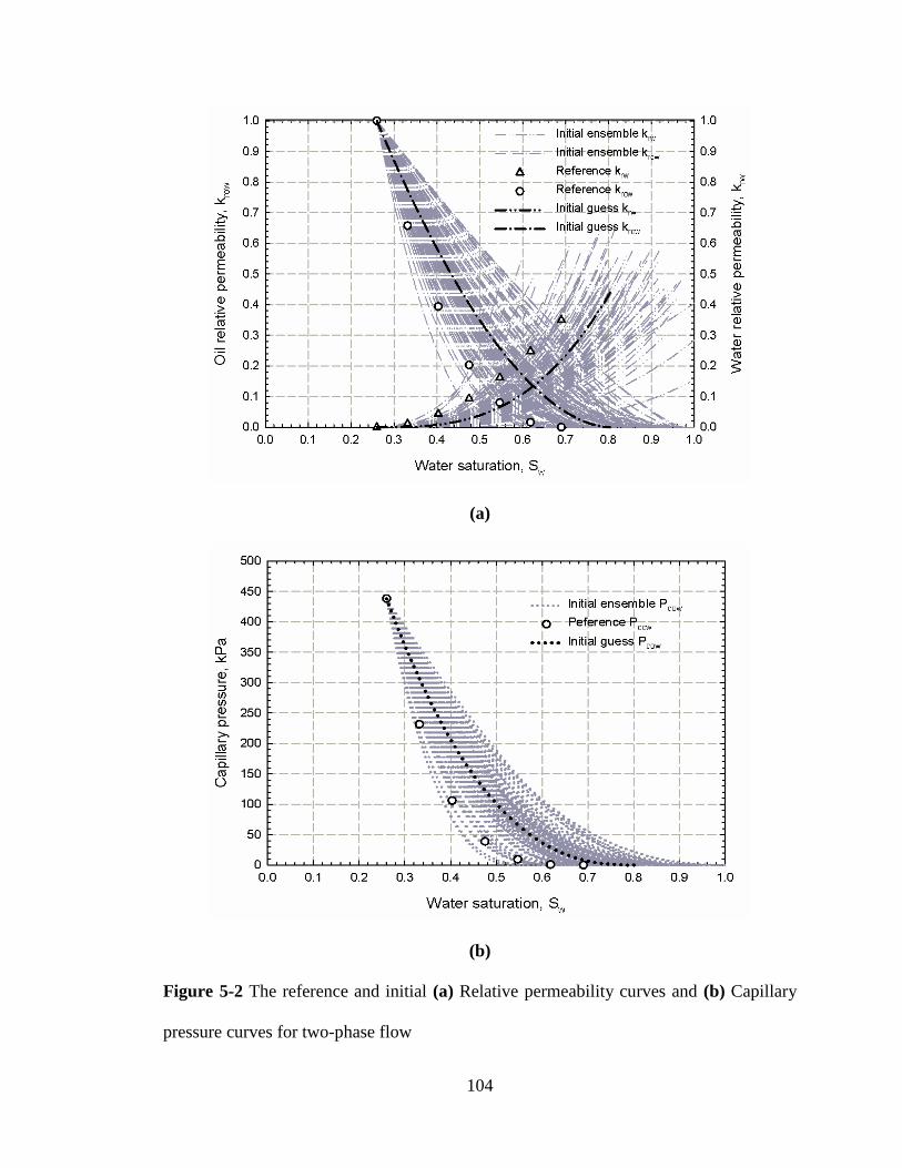
104
(a)
(b)
Figure 5-2 The reference and initial (a) Relative permeability curves and (b) Capillary
pressure curves for two-phase flow

105
(a)
(b)
Figure 5-3 The ensemble of (a) Initial water-oil ratio profiles and (b) Initial cumulative
oil production profiles of Well Pro1

106
(a)
(b)
Figure 5-4 The ensemble of (a) Initial water-oil ratio profiles and (b) Initial cumulative
oil production profiles of Well Pro2

107
(a)
(b)
Figure 5-5 The ensemble of (a) Initial water-oil ratio profiles and (b) Initial cumulative
oil production profiles of Well Pro3

108
(a)
(b)
Figure 5-6 The ensemble of (a) Initial water-oil ratio profiles and (b) Initial cumulative
oil production profiles of Well Pro4

109
dramatically so that the history matching process has mitigated uncertainties of the
relative permeability and capillary pressure curves greatly.
Figure 5-7 describes the evolution of the to-be-estimated parameters versus time. It
can be found that there are significant uncertainties with the to-be-estimated parameters
at early stage of the assimilation process, though they are generally reduced as time
proceeds. Eventually, the parameters converge to their corresponding final values, while
the variances are reduced significantly. As can be seen from Table 5-1 and Figure 5-7,
the variance values (i.e., uncertainties) of the parameters are reduced significantly
compared with their initial values after updating, though the updated ncow still has a
larger variance value than the other updated parameters, implying that the estimation
result of ncow is not as accurate as the other parameters. This may be resulted from the
fact that ncow is less sensitive to the production data, while this finding is consistent with
that in previous chapters.
The reference and updated average relative permeability and capillary pressure curves
are plotted in Figure 5-8, where the grey-shadows are the corresponding ensemble of Ne
updated relative permeability and capillary pressure curves. The updated average curves
are generated from the finally determined parameters. There exists an excellent
agreement between the reference and updated average relative permeability and capillary
pressure curves, while their uncertainty ranges are reduced significantly compared with
their initial cases as shown in Figure 5-2. However, the updated capillary pressure curves
have a relatively larger uncertainty range than the updated relative permeability curves
due to their less sensitivity to the production data.
Excellent history matching results have been obtained for each production well.

110
(a) (b)
(c) (d)
(e)
Figure 5-7 (a) aw, (b) nrw, (c) nrow, (d) ncow and (e) Sorw as a function of assimilation time
for two-phase flow
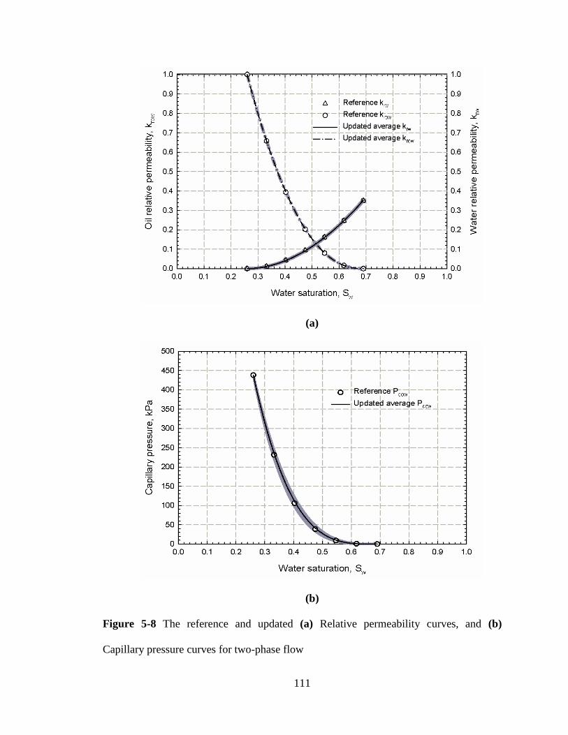
111
(a)
(b)
Figure 5-8 The reference and updated (a) Relative permeability curves, and (b)
Capillary pressure curves for two-phase flow

112
The history matching results of water-oil ratio and cumulative oil production for each
production well are respectively plotted in Figure 5-9 − Figure 5-12, where grey shadows
are ensembles of the updated water-oil ratio profiles and cumulative oil production
profiles for each production well calculated from the ensemble of Ne sets of updated
relative permeability and capillary pressure curves. The updated average water-oil ratio
and cumulative oil production of each production well are generated from the set of
updated average relative permeability and capillary pressure curves, indicating an
excellent match with their corresponding reference data. Compared with their initial
cases respectively shown in Figure 5-3 − Figure 5-6, the ensembles of the updated water-
oil ratio profiles and updated cumulative oil production profiles are all approaching their
corresponding reference data, while their uncertainty ranges are all decreased greatly due
to the significantly reduced uncertainties associated with the updated relative
permeability and capillary pressure curves.
5.3.2 Three-phase flow
The three-phase relative permeability and capillary pressure curves are estimated by
history matching the production data including oil production rate, water production rate,
gas production rate, and cumulative oil production of each well. The initial relative
permeability and capillary pressure of the oil-water system and the gas-oil system are
generated according to the initialization method as shown in Figure 5-13 and Figure 5-14,
respectively. Clearly, there exist large uncertainty ranges associated with the relative
permeability and capillary pressure curves at the beginning. Then, ensembles of initial
production profiles for each well are obtained by running the reservoir simulator with the

113
(a)
(b)
Figure 5-9 History matching results of (a) Water-oil ratio and (b) Cumulative oil
production of Well Pro1 for two-phase flow

114
(a)
(b)
Figure 5-10 History matching results of (a) Water-oil ratio and (b) Cumulative oil
production of Well Pro2 for two-phase flow
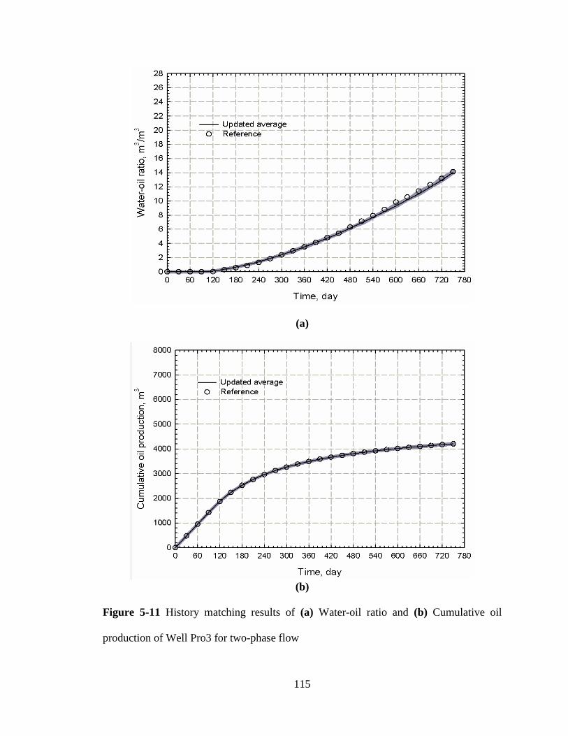
115
(a)
(b)
Figure 5-11 History matching results of (a) Water-oil ratio and (b) Cumulative oil
production of Well Pro3 for two-phase flow
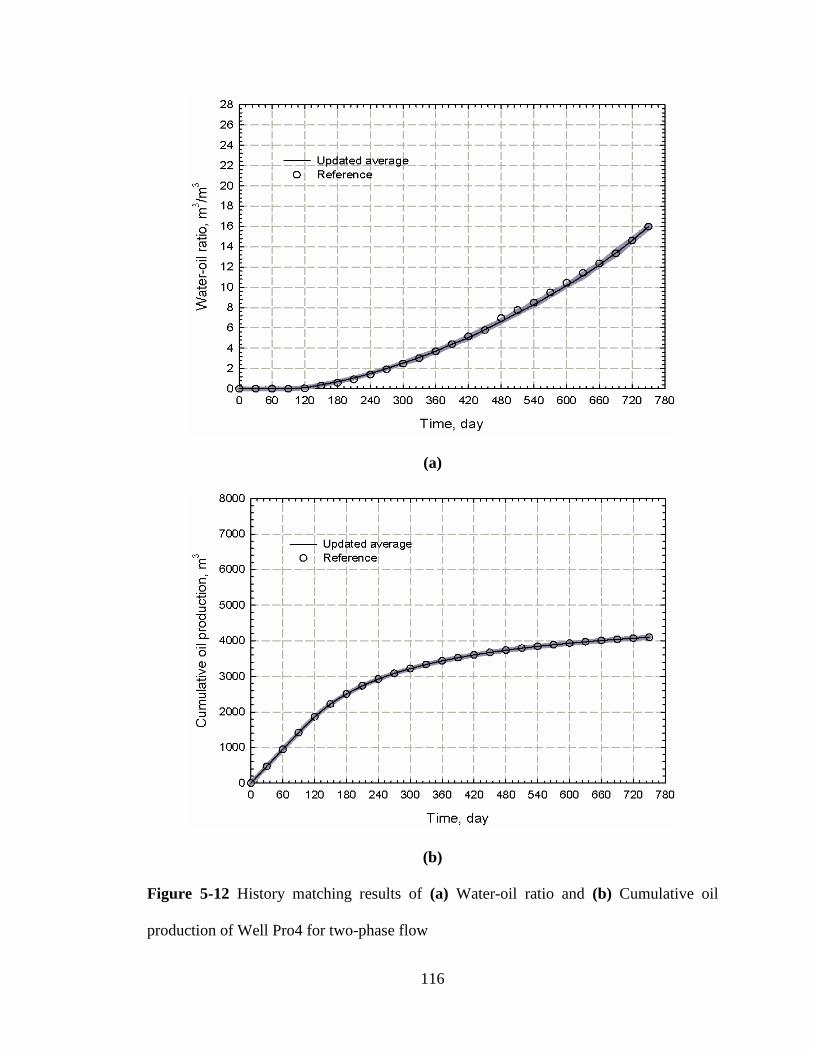
116
(a)
(b)
Figure 5-12 History matching results of (a) Water-oil ratio and (b) Cumulative oil
production of Well Pro4 for two-phase flow

117
(a)
(b)
Figure 5-13 The reference and initial (a) Relative permeability curves and (b) Capillary
pressure curves of the oil-water system in three-phase flow

118
(a)
(b)
Figure 5-14 The reference and initial (a) Relative permeability curves and (b) Capillary
pressure curves of the gas-oil system in three-phase flow

119
ensemble of initial relative permeability and capillary pressure curves, which are
respectively shown in Figure 5-15 − Figure 5-22. As can be seen, there exist wide
uncertainty ranges associated with the ensembles of initial production profiles due to the
large uncertainties in the initial relative permeability and capillary pressure curves.
Meanwhile, the reference production data are all respectively covered by their
corresponding ensembles of initial production profiles.
The finally determined parameters are tabulated in Table 5-2. Similar to the two-
phase flow, standard deviations of the updated parameters are reduced dramatically
throughout the history matching process, implying that uncertainties of the relative
permeability and capillary pressure have been greatly mitigated. The evolution processes
of the to-be-estimated parameters used to generate relative permeability and capillary
pressure curves for the oil-water system and gas-oil system is respectively plotted in
Figure 5-23 and Figure 5-24. Significant uncertainties are found to be associated with
these parameters at early stage of the assimilation process, though they are generally
reduced as time proceeds. Eventually, all of the parameters converge to the final
determined values. Although the variance values of all the updated parameters have been
reduced significantly, the exponents of capillary pressure curves (i.e., ncow and ncog) still
have relatively larger variance values than the other parameters after updating. This
implies that capillary pressure is still less sensitive to the production data in tight
formations compared with the relative permeability.
Figure 5-25 and Figure 5-26 respectively depict the reference and updated average
relative permeability and capillary pressure curves for the oil-water system and gas-oil
system, where the grey-shadows are the corresponding ensemble of Ne updated relative
permeability and capillary pressure curves. The updated average relative permeability
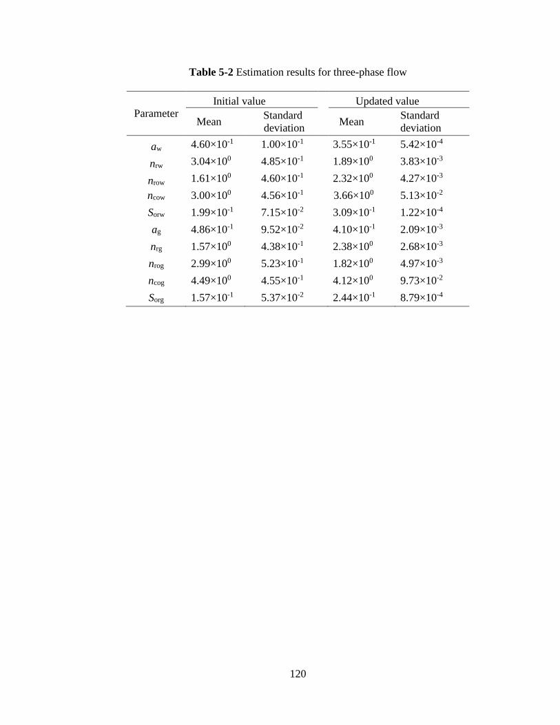
120
Table 5-2 Estimation results for three-phase flow
Parameter Initial value Updated value
Mean Standard
deviation Mean
Standard
deviation
aw 4.60×10⁻¹ 1.00×10⁻¹ 3.55×10⁻¹ 5.42×10⁻⁴
nrw 3.04×100 4.85×10⁻¹ 1.89×100 3.83×10⁻³
nrow 1.61×100 4.60×10⁻¹ 2.32×100 4.27×10⁻³
ncow 3.00×100 4.56×10⁻¹ 3.66×100 5.13×10⁻²
Sorw 1.99×10⁻¹ 7.15×10⁻² 3.09×10⁻¹ 1.22×10⁻⁴
ag 4.86×10⁻¹ 9.52×10⁻² 4.10×10⁻¹ 2.09×10⁻³
nrg 1.57×100 4.38×10⁻¹ 2.38×100 2.68×10⁻³
nrog 2.99×100 5.23×10⁻¹ 1.82×100 4.97×10⁻³
ncog 4.49×100 4.55×10⁻¹ 4.12×100 9.73×10⁻²
Sorg 1.57×10⁻¹ 5.37×10⁻² 2.44×10⁻¹ 8.79×10⁻⁴
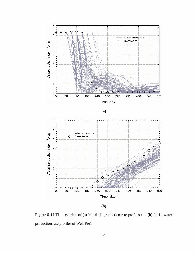
121
(a)
(b)
Figure 5-15 The ensemble of (a) Initial oil production rate profiles and (b) Initial water
production rate profiles of Well Pro1
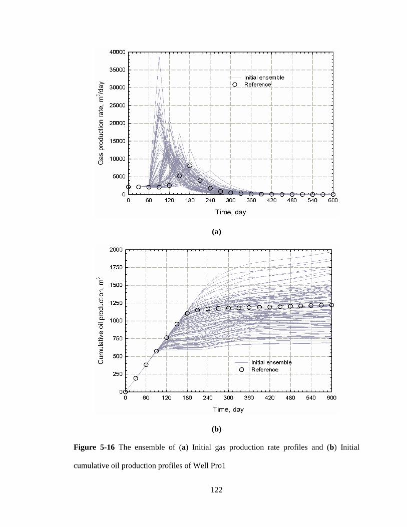
122
(a)
(b)
Figure 5-16 The ensemble of (a) Initial gas production rate profiles and (b) Initial
cumulative oil production profiles of Well Pro1
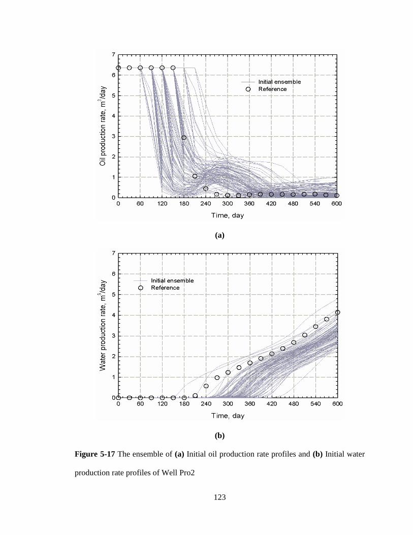
123
(a)
(b)
Figure 5-17 The ensemble of (a) Initial oil production rate profiles and (b) Initial water
production rate profiles of Well Pro2
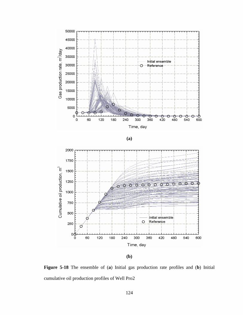
124
(a)
(b)
Figure 5-18 The ensemble of (a) Initial gas production rate profiles and (b) Initial
cumulative oil production profiles of Well Pro2
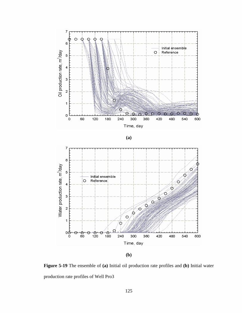
125
(a)
(b)
Figure 5-19 The ensemble of (a) Initial oil production rate profiles and (b) Initial water
production rate profiles of Well Pro3
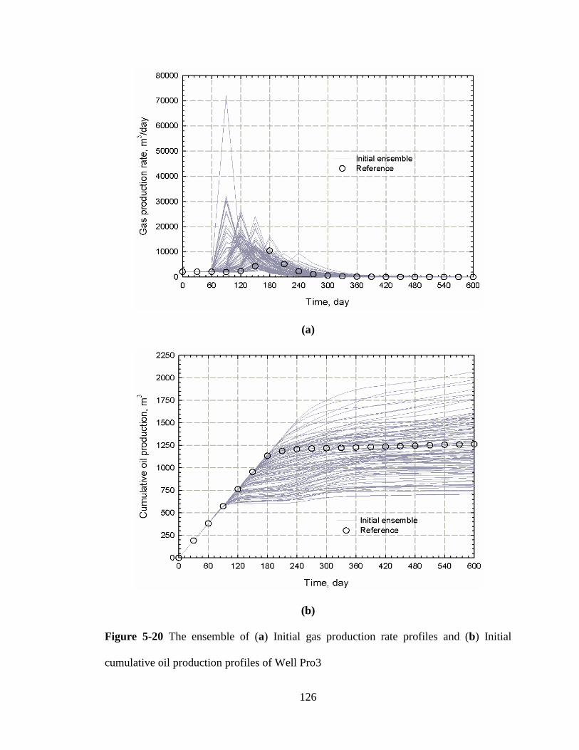
126
(a)
(b)
Figure 5-20 The ensemble of (a) Initial gas production rate profiles and (b) Initial
cumulative oil production profiles of Well Pro3

127
(a)
(b)
Figure 5-21 The ensemble of (a) Initial oil production rate profiles and (b) Initial water
production rate profiles of Well Pro4
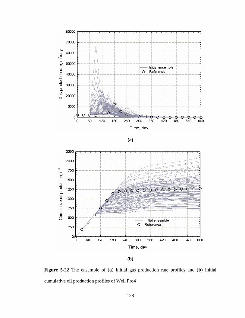
128
(a)
(b)
Figure 5-22 The ensemble of (a) Initial gas production rate profiles and (b) Initial
cumulative oil production profiles of Well Pro4

129
(a) (b)
(c) (d)
(e)
Figure 5-23 (a) aw, (b) nrw, (c) nrow, (d) ncow and (e) Sorw as a function of assimilation
time in three-phase flow

130
(a) (b)
(c) (d)
(e)
Figure 5-24 (a) ag, (b) nrg, (c) nrog, (d) ncog and (e) Sorg as a function of assimilation time
in three-phase flow
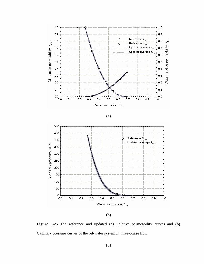
131
(a)
(b)
Figure 5-25 The reference and updated (a) Relative permeability curves and (b)
Capillary pressure curves of the oil-water system in three-phase flow
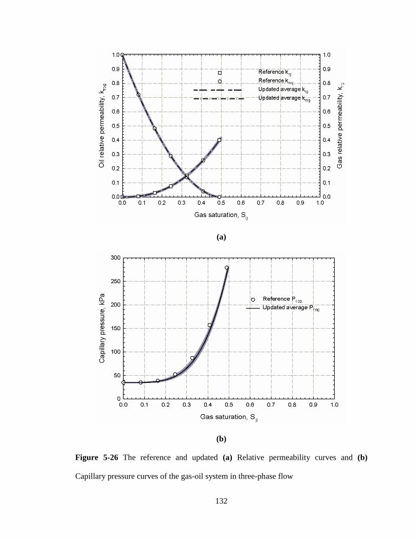
132
(a)
(b)
Figure 5-26 The reference and updated (a) Relative permeability curves and (b)
Capillary pressure curves of the gas-oil system in three-phase flow

133
and capillary pressure curves are in an excellent agreement with the corresponding
reference curves after assimilating all of the reference production data, while their
uncertainty ranges are reduced significantly compared with the corresponding initial
cases as shown in Figure 5-13 and Figure 5-14, respectively. However, the end-point of
gas relative permeability curve (i.e., ag) is overestimated slightly, while the gas-oil
capillary pressure curves deviate from the reference curve slightly at a high gas
saturation. These may be ascribed to the fact that the production data contains
information mainly reflecting a low gas saturation released from the oil. Another reason
for such a minor mismatch may be attributed to the fact that the capillary pressure is less
sensitivity to the production data.
Excellent history matching results have been obtained for all producers, which are
respectively depicted in Figure 5-27 − Figure 5-34. The grey shadows are the
corresponding ensembles of the updated production profiles calculated from the
ensemble of updated relative permeability and capillary pressure curves, while the
updated average production profiles are generated from the set of the updated average
relative permeability and capillary pressure curves. Obviously, after assimilating all the
reference production data, the updated production profiles agree well with the reference
values, though there is a minor mismatch for the gas-oil capillary pressure curves. This
further supports the finding that the capillary pressure is less sensitive to the production
data as mentioned previously. Similar to the two-phase flow, the uncertainty ranges
associated with the updated production profiles are all decreased greatly due to the
significantly reduced uncertainties associated with the updated relative permeability and
capillary pressure curves.
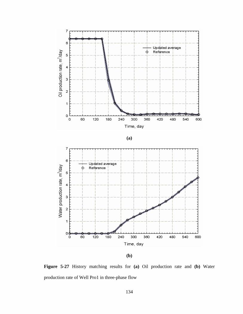
134
(a)
(b)
Figure 5-27 History matching results for (a) Oil production rate and (b) Water
production rate of Well Pro1 in three-phase flow
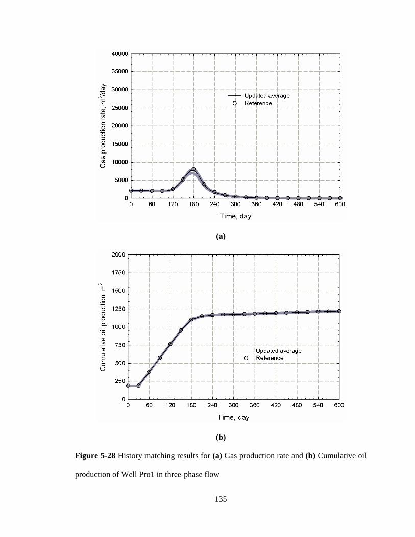
135
(a)
(b)
Figure 5-28 History matching results for (a) Gas production rate and (b) Cumulative oil
production of Well Pro1 in three-phase flow

136
(a)
(b)
Figure 5-29 History matching results for (a) Oil production rate and (b) Water
production rate of Well Pro2 in three-phase flow

137
(a)
(b)
Figure 5-30 History matching results for (a) Gas production rate and (b) Cumulative oil
production of Well Pro2 in three-phase flow
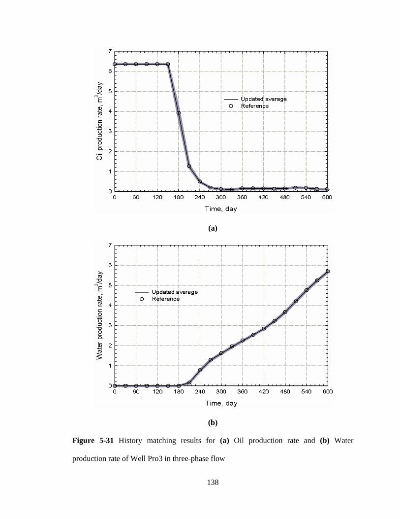
138
(a)
(b)
Figure 5-31 History matching results for (a) Oil production rate and (b) Water
production rate of Well Pro3 in three-phase flow
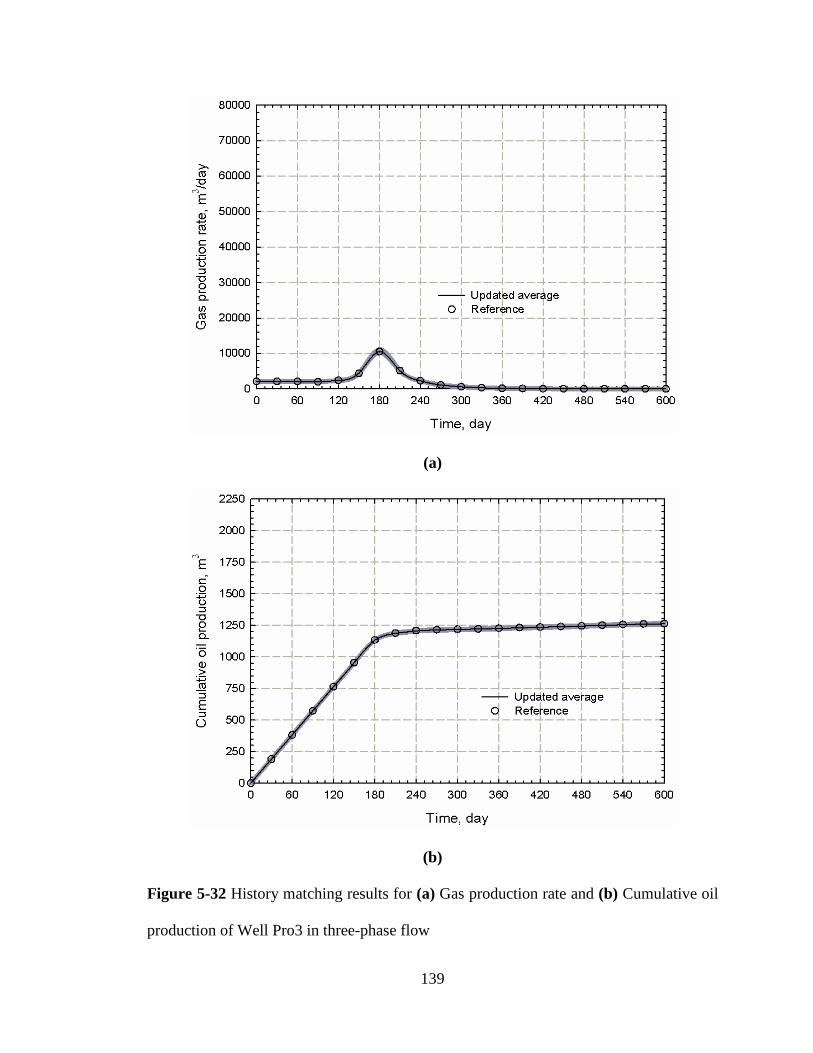
139
(a)
(b)
Figure 5-32 History matching results for (a) Gas production rate and (b) Cumulative oil
production of Well Pro3 in three-phase flow
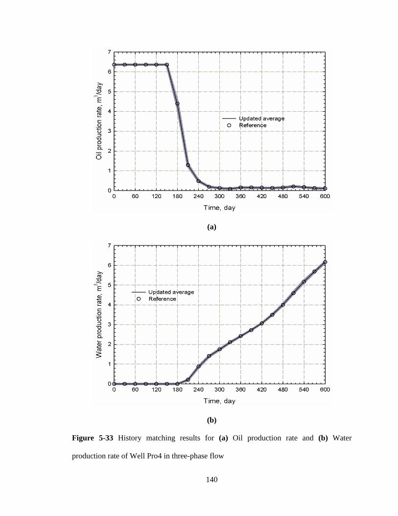
140
(a)
(b)
Figure 5-33 History matching results for (a) Oil production rate and (b) Water
production rate of Well Pro4 in three-phase flow
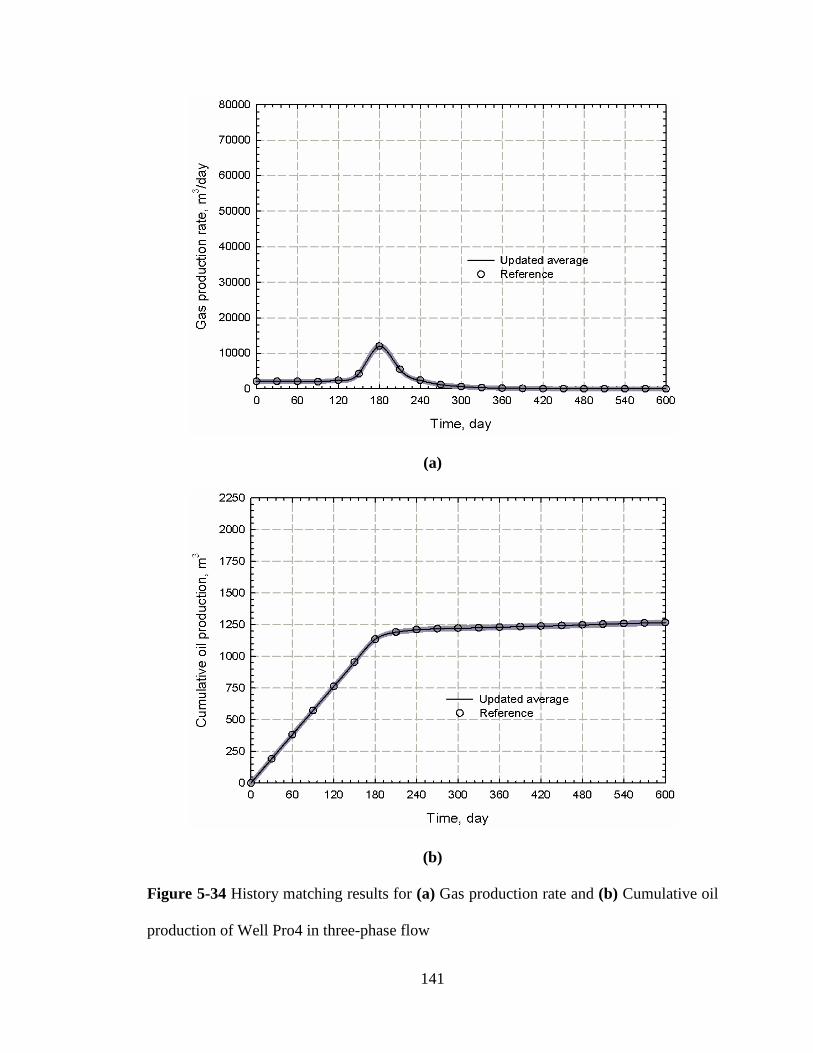
141
(a)
(b)
Figure 5-34 History matching results for (a) Gas production rate and (b) Cumulative oil
production of Well Pro4 in three-phase flow

142
5.4 Summary
The assisted history matching technique based on the EnKF algorithm has been
successfully applied to accurately evaluate relative permeability and capillary pressure
for tight formations by history matching the field production data, while it has been
validated by using a synthetic 2D heterogeneous reservoir model. Two-phase and three-
phase relative permeability and capillary pressure curves are respectively estimated,
while the power-law model is used to represent the relative permeability and capillary
pressure curves.
Generally, the relative permeability and capillary pressure curves are updated
progressively and their uncertainty is reduced gradually as more production data is
assimilated, while the capillary pressure curve cannot be determined as accurately as the
relative permeability curve due to its less sensitivity to the production data. In addition,
the uncertainty ranges associated with the updated production profiles are all reduced
greatly due to the significantly reduced uncertainties in the updated relative permeability
and capillary pressure curves.
As for two-phase flow, there exits an excellent agreement between the reference and
updated average relative permeability and capillary pressure curves, leading to an
excellent history matching results. Similarly, there exists a good agreement between the
reference and updated average relative permeability and capillary pressure curves in
three-phase flow. Although parameter ag is overestimated slightly together with a minor
mismatch for the gas-oil capillary pressure curve at the high gas saturation range due to
the fact that the production data mainly contains information at a low gas saturation
range, there still exist excellent history matching results.
143
CHAPTER 6 ESTIMATION OF RELATIVE PERMEABILITY
AND CAPILLAY PRESSURE FOR A TIGHT
FORMATION FROM DISPLACEMENT
EXPERIMENT USING A DAMPED ITERATIVE
ENKF TECHNIQUE
In this chapter, a new form of damped iterative EnKF (IEnKF) algorithm has been
proposed to improve performance of the existing EnKF algorithm with a strongly
nonlinear data assimilation system. This new technique has been successfully applied to
simultaneously estimate relative permeability and capillary pressure for the tight
formations by assimilating conventional measurement data (i.e., cumulative oil
production and pressure drop) from a coreflooding experiment, while the B-spline model
is employed to represent the relative permeability and capillary pressure curves.
6.1 Methodology
In Sections 3.2 and 4.2, it has proven that the EnKF algorithm can be used to
simultaneously estimate relative permeability and capillary pressure accurately in
conventional reservoirs and tight formations by assimilating displacement experiment
data including cumulative production data, pressure drop and saturation profiles.
However, as can be seen from Section 4.3.2, the EnKF algorithm fails to function well if
fluid saturation profile is not available to be assimilated. Although the relative
permeability and capillary pressure can be finally determined by using the EnKF
algorithm to assimilate the conventional measurement data from the laboratory
coreflooding experiment, there is certain mismatch for the history matching results,
144
especially for the cumulative oil production (see Section 4.4.2). This is because, without
fluid saturation profile, nonlinearity of the data assimilation system as a whole will be
greatly increased. In this way, the data assimilation system may become a strongly
nonlinear one where the EnKF algorithm finds its limitations (Aanonsen et al., 2009).
This is especially true for the tight formations.
In practice, the IEnKF techniques have seen some successful applications in the
strongly nonlinear data assimilation systems (Gu and Oliver, 2007; Li and Reynolds,
2009). In addition, as analyzed in Section 4.4.2, the formulaic nature of the power-law
representation may be one of the potential reasons that induce the mismatch for the
history matching results. As such, the B-spline model is used in this study to represent
the relative permeability and capillary pressure curves in a more flexible way (see
Section 4.1 for detail).
6.1.1 IEnKF algorithm
The iterative forms of Kalman filter are not entirely new, such as the iterated Kalman
filter with no ensemble (Jazwinski, 1970), while the iterative methods have already been
applied in the EnKF context (Zupanski, 2005; Wen and Chen, 2007). Such iterative
forms can be viewed as algorithms for minimizing a stochastic objective function, or
equivalently, for maximizing the posterior probability of each realization conditional to
its forecast value and the new data (Aanonsen et al., 2009). For example, Gu and Oliver
(2007) proposed an iterative EnKF based on a randomized maximum likelihood filter
called the ensemble randomized maximum likelihood filter (EnRML). The EnRML is
based on the iterative solution for the minimum of a quadratic cost function by the

145
Newton method, while it has shown better performance for the nonlinear and non-
Gaussian data assimilation problems. In this chapter, a new form of the IEnKF method
(i.e., a further development of the EnRML) has been introduced to incorporate the
ensemble square root filter (ESRF) as the linear solution during the iterative process,
while its basic updating function can be expressed as (Sakov et al., 2012),
iiiiii1
01
101
111122obs,2121
11 XXCCXdKXX
MH [6-1]
where subscripts 1 and 2 respectively represent variables at time t1 and time t2 where
new measurement data is available to be assimilated. The superscript i is the iteration
index referring to i+1th iteration step, while i = 0 represents the initial state. X is the
model-state estimate which is the ensemble mean. 01X is the initial model-state estimate
in the current data assimilation cycle, which is the finally updated model-state estimate
from the previous assimilation cycle. The finally updated model-state estimate of the
current cycle is denoted as X2 which will be used as the initial model-state estimate in the
next cycle. 01C is the initial model-state error covariance prior to assimilating any new
measurement data at time t2, while 1
1iC is the estimated model-state error covariance at
the i+1th iteration step. i12K is the Kalman gain, which is the sensitivity of the analysis at
time t1 to the innovation at time t2. obs,2d is the new measurement data available at time t2
associated with measurement error covariance Cdd. 2H is the observation operator at time
t2, so X2H represents the simulated measurement data at time t2 associated with the
model-state estimate X at that time. 12M is the nonlinear propagator from time t1 to t2,
which is a reservoir simulator (i.e., CMG IMEX 2010.10) in this study, so that,
1122 XX M [6-2]

146
As for the gradient-based history matching techniques, it has been proven that it is
important to damp the larger updated value at early iterations for larger mismatch (Li et
al., 2003; Gao and Reynolds, 2006), while it is also important to damp the larger update
at early iterations for the iterative ensemble-based methods (Wen and Chen, 2007; Chen
and Oliver, 2012). Without damping, the larger modifications introduced at early
iterations will not always be removed at later iterations, and thus it is more likely to lead
to a local minimum. As such, it is better to perform damping with iterations for the new
IEnKF algorithm, while the improved IEnKF method with a damped updating is
proposed as follows,
iiiiiiii1
01
101
111122obs,2121
11 XXCCXdKXX
MH [6-3]
where i is the damping parameter with a value between 0 and 1. In practice, it is
difficult to select the damping parameter value, depending on the degree of the
nonlinearity of the problem and the level of non-Gaussian property of the measurement
error. In most cases, it is still determined by using the trial-and-error method. Most
recently, Chen and Oliver (2012) have proven that the choice of β value between 0.4 and
0.5 would provide the smallest mismatch after the first iteration. As such, the value of β
in the first iteration (i.e., 0 ) is chosen to be 0.45 in this study, while the value of β in
the subsequent iteration will be tuned according to the degree of data mismatch after
previous iteration.
6.1.2 IEnKF implementation
As for the ensemble-based methods, the model-state is characterized by an ensemble of
model realizations em NN E , where Nm is the size of each model realization and Ne is the
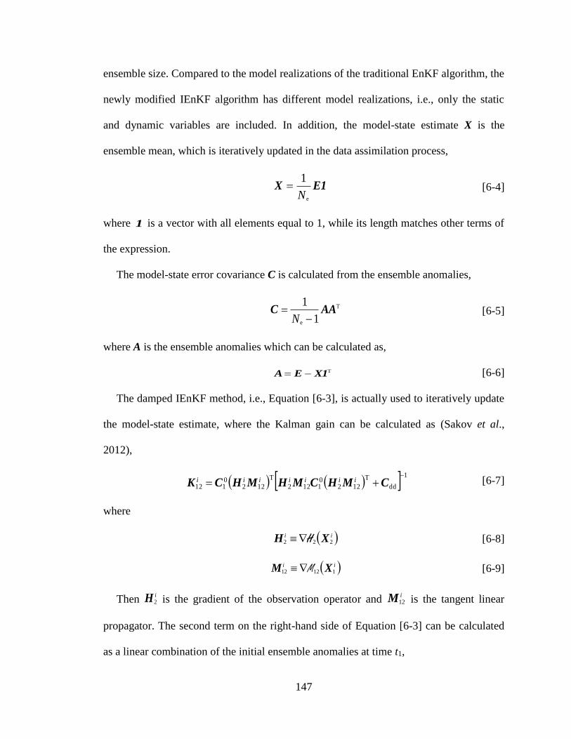
147
ensemble size. Compared to the model realizations of the traditional EnKF algorithm, the
newly modified IEnKF algorithm has different model realizations, i.e., only the static
and dynamic variables are included. In addition, the model-state estimate X is the
ensemble mean, which is iteratively updated in the data assimilation process,
E1Xe
1
N [6-4]
where 1 is a vector with all elements equal to 1, while its length matches other terms of
the expression.
The model-state error covariance C is calculated from the ensemble anomalies,
T
e 1
1AAC
N [6-5]
where A is the ensemble anomalies which can be calculated as,
TX1EA [6-6]
The damped IEnKF method, i.e., Equation [6-3], is actually used to iteratively update
the model-state estimate, where the Kalman gain can be calculated as (Sakov et al.,
2012),
1
dd
T
12201122
T
1220112
CMHCMHMHCK iiiiiii [6-7]
where
ii222 XH H [6-8]
ii11212 XM M [6-9]
Then i2H is the gradient of the observation operator and
i12M is the tangent linear
propagator. The second term on the right-hand side of Equation [6-3] can be calculated
as a linear combination of the initial ensemble anomalies at time t1,

148
iiiii2
011122obs,212 bAXdK MH [6-10]
where 01A is the initial ensemble anomalies and
i2b is a vector of linear coefficients
which can be expressed via the standardized ensemble observation anomalies i2S and
standardized innovation i2s (Sakov et al., 2012),
iiiii2
T
2
1
2
T
22 sSSSIb
[6-11]
where I is an identity matrix and,
1e
01122
2
1
dd
2
N
ii
i AMHCS [6-12]
1e
1122obs,22
1
dd
2
N
i
i XdCs
MH [6-13]
where 01122 AMH ii
can be interpreted as the initial ensemble anomalies propagated with
current estimated i12M and observed with current estimated
i2H , which can be
approximated as (Sakov et al., 2012),
1
2T
e
112201122
1
iiii
NG11IEAMH MH [6-14]
where i2G is an ensemble transform matrix calculated at time t2 to estimate the ensemble
anomalies at time t1 (Sakov et al., 2012),
2
1
12
T122
iii SSIG [6-15]
and i1E is the ensemble of the updated model realizations after previous iteration,
iii1
T11 A1XE [6-16]

149
where i1A is the estimated ensemble anomalies after previous iteration, which can be
estimated as (Sakov et al., 2012),
ii2
011 GAA [6-17]
Finally, the third term on the right hand side of Equation [6-3] can be estimated as,
iiiiii
iiii
iiiiiii
101
T01
01
T01
T
2
1
2
T
22
1
2
T
201
101
T01
01
T01
T12
12
01
101
T01
01
T11
111
01
101
11
XXAAASSISSIA
XXAAAGGA
XXAAAAXXCC
[6-18]
where the symbol denotes a pseudo-inverse.
Except for the iteration process, the damped IEnKF procedure is similar to that of the
EnKF algorithm. The procedure of the damped IEnKF algorithm proposed in this chapter
is briefly described as follows:
(1). Initialization
The ensemble of the updated model realizations from the previous assimilation
cycle is used as the ensemble of initial model realizations 01E in the current
assimilation cycle, while the initial model-state estimate 01X and the initial
ensemble anomalies 01A in the current cycle are calculated with Equations [6-4]
and [6-6], respectively. Meanwhile, the initial ensemble transform matrix 02G is
set to be an identity matrix and 45.00 ;
150
(2). Iteration
2.1). Forecasting: To advance the ensemble of the updated model realizations
obtained from previous iteration using the nonlinear propagator 12M (i.e., a
reservoir simulator) from time t1 to time t2 where new measurement data is
available to be assimilated. Note that, in this study, the reservoir simulator is re-
run from initial time t = 0 instead of re-running from time t1 to time t2, which is an
additional “confirming step” to guarantee that the updated static and dynamic
variables are always consistent.
2.2). Calculating increments: To assemble the simulated measurement data (i.e.,
i1122 EMH ) from each model realization at time t2, while the simulated
measurement data generated from the model-state estimate, i
1X , can be
approximated as,
e
11221122
N
ii 1E
XM
MH
H [6-19]
Then, 01122 AMH ii
is approximated by using Equation [6-14], while i2S and
i2s are
calculated using Equations [6-12] and [6-13], respectively. Subsequently, i2b and
12iG can be calculated using Equations [6-11] and [6-15], respectively. Finally,
the increments are estimated by Equations [6-10] and [6-18], respectively.
2.3). Updating: To apply Equations [6-3] and [6-17] to respectively update the
model-state estimate1
1iX and ensemble anomalies
11iA , while the ensemble of
the updated model realizations 1
1iE is determined by using Equation [6-16].

151
2.4). Evaluating the mismatch: To calculate the data mismatch for both i1E and
11iE by using,
obs,2ksim,1
dd
1
T
obs,2ksim,
de
1
e1ddCddE
N
kNNS [6-20]
where Nd is the number of measurement data and ksim,d is the simulated
measurement data at time t2 calculated from the kth model realization.
2.5). Choosing the updating results and value: If 11iS E < iS 1E , overwrite
i1X
and i1E with
11iX and
11iE , respectively. Then the value of is increased in the
next iteration; otherwise, keep i1X and
i1E while decreasing the value of for
the next iteration.
2.6). Examining convergence criteria: If the convergence criterion has not been
satisfied, return to Step #2.1 to repeat the iteration; otherwise, exit this iteration
and go to Step #3.
(3). Output
If there is an additional set of new measurement data available, return to Step #1
until all the measurement data are assimilated; otherwise, output the final results.
The convergence criteria used in this study to determine if the solution has converged
include:
(a). The maximum change criterion (i.e., 1
1,1,
1
,es
MAX
NlNm
i
lm
i
lm MM ) of the
estimated reservoir parameters between two sequential iterations is smaller than
152
a pre-specified value 1 = 1×10⁻³. es NN M is the ensemble of to-be-estimated
reservoir parameters and lmM , is corresponding to
lmE ,; Ns is the number of to-
be-estimated reservoir parameters.
(b). To meet
2
1
11
1
i
ii
S
SS
E
EE, where 2 = 1×10⁻².
(c). Exceed the pre-specified maximum iteration number (MI): MI = 30 in this study.
6.2 Case Study
In this section, the newly proposed damped IEnKF algorithm is applied to the laboratory
coreflooding experiment which has been described in detail in Section 4.3.2, while its
numerical simulation model built in Section 4.3.2 is also used in this study. The
simulated measurement data only include cumulative oil production and pressure drop,
while the model realization of the damped IEnKF method only includes dynamic and
static variables. In this study, the dynamic variables in each model realization include
grid pressure and water saturation of each grid.
The B-spline model is used to represent the relative permeability and capillary
pressure curves more flexibly in this study. In order to both ensure the updated curves to
be monotonic and keep the flexible characteristics of the B-spline representation, the
control knots on each curve are transformed to their corresponding pseudo-control knots
which are to be tuned during the data assimilation process by using Equation [4-6].
Therefore, the static variables include pseudo-control knots of relative permeability and
capillary pressure curves, irreducible water saturation Swi, and residual oil saturation Sorw.

153
The relative permeability and capillary pressure curves are divided into ten sections
(i.e., n = 10) uniformly in this study. Thus, there are eleven control knots on each curve.
In general, the oil relative permeability at irreducible water saturation can be normalized
to be 1.0 (i.e., row0C = 1), while oil relative permeability is zero at residual oil saturation
(i.e., rownC = 0). As such, these two control knots will not be the to-be-estimated model
parameters. Then, there are nine to-be-estimated control knots for oil relative
permeability curve, which are corresponding to nine pseudo-control knots to be tuned
during the data assimilation process. Since water relative permeability is equal to zero at
irreducible water saturation (i.e., rw0C = 0), there are ten to-be-estimated control knots for
water relative permeability curve, which are corresponding to ten to-be-tuned pseudo-
control knots.
As mentioned in Section 4.3.2, the capillary pressure at irreducible water saturation
(i.e., cow0C ) and the capillary pressure at residual oil saturation (i.e.,
cownC ) can be scaled
by using the J-function according to prior knowledge, whose values are determined to be
547.17 kPa and 281.42 kPa, respectively. Thus, there are nine to-be-estimated control
knots for capillary pressure curve, which are corresponding to nine to-be-tuned pseudo-
control knots. As such, the static variables to be tuned during the data assimilation
process can be expressed as,
],,,...,,,,...,,,,...,,[ orwwicow9
cow2
cow1
rw10
rw2
rw1
row9
row2
row1 SSxxxxxxxxx [6-21]
At initial time, the model-state should be initialized according to prior knowledge,
while the initialization process has been described in Section 4.2. In this study, the
irreducible water saturation and residual oil saturation calculated directly from the
coreflooding experiment are set to be the initial guess for the Swi and Sorw, respectively.

154
6.3 Results and Discussion
At initial time, a set of initial guess relative permeability and capillary pressure curves is
assigned according to prior knowledge (see Figure 6-1a and b), where the solid symbols
on each curve are the initial guess control knots to interpolate the corresponding curves,
while an ensemble of Ne sets of initial relative permeability and capillary pressure curves
are generated according to the initialization process mentioned previously. As can be
seen, there are large uncertainty ranges respectively associated with the initial relative
permeability and capillary pressure curves before assimilating any measurement data.
Then, an ensemble of initial cumulative oil production profiles and an ensemble of
initial pressure drop profiles are obtained by running the reservoir simulator with the
ensemble of Ne sets of initial relative permeability and capillary pressure curves, which
are shown in Figure 6-2a and b, respectively. Obviously, there exist wide uncertainty
ranges respectively associated with the ensembles of initial cumulative oil production
profiles and initial pressure drop profiles due to the large uncertainties in the initial
relative permeability and capillary pressure curves. Meanwhile, the measured cumulative
oil production and pressure drop are all covered by the ensembles of initial cumulative
oil production profiles and initial pressure drop profiles, respectively.
Finally, the relative permeability and capillary pressure curves are determined by
assimilating all of the experimental measurement data as depicted in Figure 6-3a and b,
respectively, where the grey shadows are the ensembles of Ne updated relative
permeability and capillary pressure curves. The updated average curves are interpolated
from the updated average control knots whose values are the mean of the updated
ensemble members. As can be seen, the uncertainty ranges associated with the updated

155
(a)
(b)
Figure 6-1 (a) Initial relative permeability curves and (b) Initial capillary pressure
curves using IEnKF algorithm

156
(a)
(b)
Figure 6-2 The ensemble of (a) Initial cumulative oil production profiles and (b) Initial
pressure drop profiles
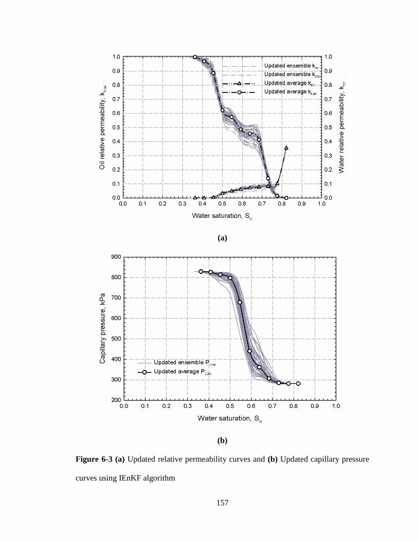
157
(a)
(b)
Figure 6-3 (a) Updated relative permeability curves and (b) Updated capillary pressure
curves using IEnKF algorithm

158
relative permeability and capillary pressure curves have been significantly reduced
compared with the corresponding initial cases. However, the uncertainty ranges of the
updated curves between the water saturation of 0.5 and 0.7 which may be corresponding
to the water breakthrough period, especially on the updated oil relative permeability
curves, are relatively larger than the other sections of the updated curves. This may be
resulted from the instability during the water breakthrough period and less measurement
data available to be assimilated in this period. Besides, it can be seen that the uncertainty
range of the updated water relative permeability curves is smaller than those of the
updated oil relative permeability and capillary pressure curves. This phenomenon further
confirms the finding that water relative permeability is more sensitive to the
measurement data than the oil relative permeability and capillary pressure in previous
studies.
The history matching results of cumulative oil production and pressure drop are
plotted in Figure 6-4a and b, respectively, where grey shadows are the ensembles of
updated cumulative oil production and pressure drop profiles calculated from the
ensemble of Ne sets of updated relative permeability and capillary pressure curves. The
updated average cumulative oil production and pressure drop are generated from the
updated average relative permeability and capillary pressure curves, indicating an
excellent match with their corresponding measurement data.
Compared with the initial cases respectively shown in Figure 6-2a and b, ensembles
of the updated cumulative oil production and pressure drop profiles are all approaching
their corresponding measurement data, while their uncertainty ranges are all decreased
greatly owing to the significantly reduced uncertainties associated with the updated

159
(a)
(b)
Figure 6-4 The ensemble of (a) Updated cumulative oil production profiles and (b)
Updated pressure drop profiles
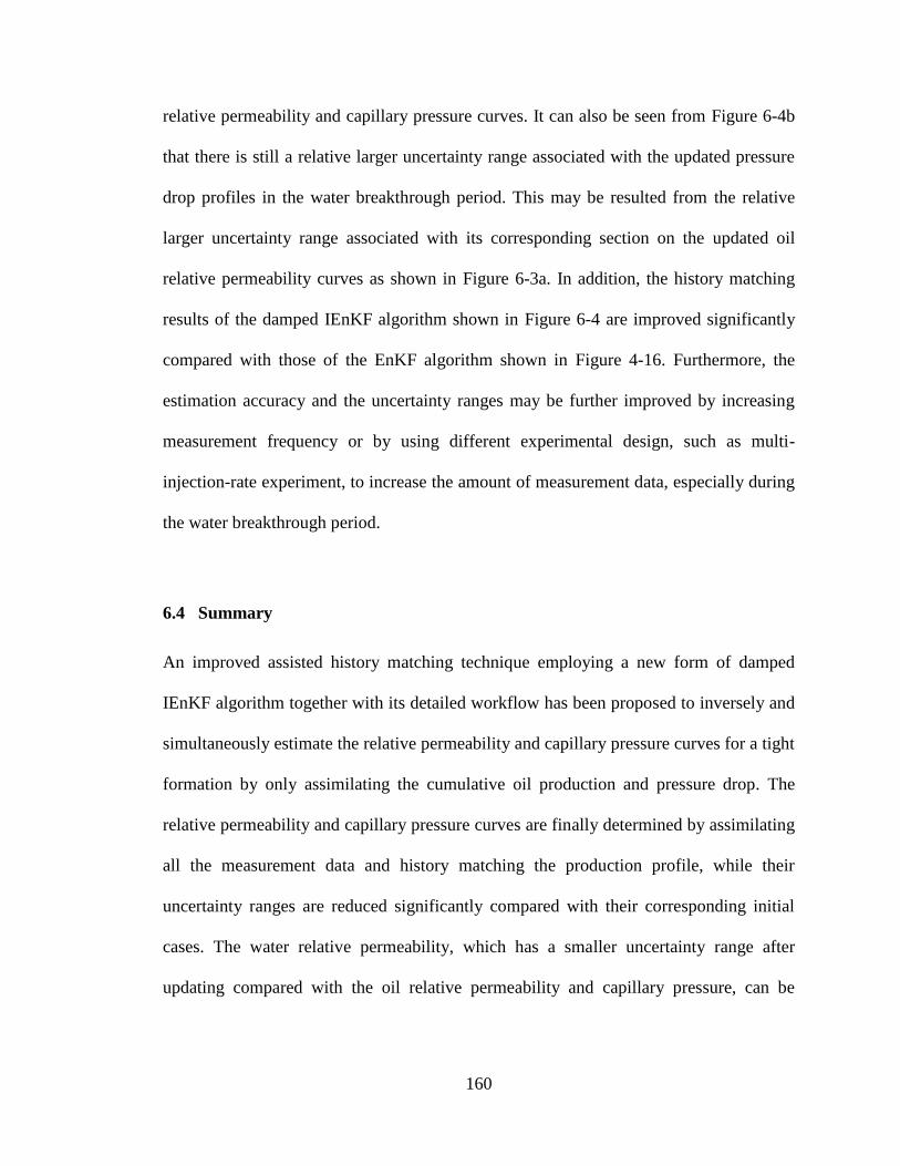
160
relative permeability and capillary pressure curves. It can also be seen from Figure 6-4b
that there is still a relative larger uncertainty range associated with the updated pressure
drop profiles in the water breakthrough period. This may be resulted from the relative
larger uncertainty range associated with its corresponding section on the updated oil
relative permeability curves as shown in Figure 6-3a. In addition, the history matching
results of the damped IEnKF algorithm shown in Figure 6-4 are improved significantly
compared with those of the EnKF algorithm shown in Figure 4-16. Furthermore, the
estimation accuracy and the uncertainty ranges may be further improved by increasing
measurement frequency or by using different experimental design, such as multi-
injection-rate experiment, to increase the amount of measurement data, especially during
the water breakthrough period.
6.4 Summary
An improved assisted history matching technique employing a new form of damped
IEnKF algorithm together with its detailed workflow has been proposed to inversely and
simultaneously estimate the relative permeability and capillary pressure curves for a tight
formation by only assimilating the cumulative oil production and pressure drop. The
relative permeability and capillary pressure curves are finally determined by assimilating
all the measurement data and history matching the production profile, while their
uncertainty ranges are reduced significantly compared with their corresponding initial
cases. The water relative permeability, which has a smaller uncertainty range after
updating compared with the oil relative permeability and capillary pressure, can be

161
estimated more accurately owing to the fact that it is more sensitive to the measurement
data.
There exist excellent history matching results between both the updated average
cumulative oil production and pressure drop and their corresponding measurement data,
while the uncertainty ranges associated with the updated cumulative oil production and
pressure drop profiles are reduced greatly due to the significantly reduced uncertainties
in the updated relative permeability and capillary pressure curves. Such damped IEnKF
algorithm has proven to perform better than the confirming EnKF algorithm in the
laboratory coreflooding experiment, while it is special suitable for strongly nonlinear
data assimilation system. In addition, the new technique is also easy to be implemented
and well-suited for uncertainty analysis under a consistent framework.
162
CHAPTER 7 SIMULTANEOUS ESTIMATION OF RELATIVE
PERMEABILITY AND CAPILLARY PRESSURE
FOR PUNQ-S3 MODEL WITH THE DAMPED
IENKF TECHNIQUE
In this chapter, the newly proposed damped IEnKF algorithm and CMOST (CMG
2010.10) have been applied to simultaneously estimate three-phase relative permeability
and capillary pressure curves by history matching long-term field production data from a
standard test model, i.e., the PUNQ-S3 reservoir model, which is based on a real field.
7.1 Methodology
The traditional and confirming EnKF techniques have found their limitations in large-
scale history matching problems due to the nature of strong nonlinearity (Aanonsen et al.,
2009), while the IEnKF techniques have seen some successful applications in the full
field history matching problems (Gu and Oliver, 2007; Li and Reynolds, 2009; Chen and
Oliver, 2013). Although the damped IEnKF algorithm proposed in CHAPTER 6 has
shown great potential in the strongly nonlinear data assimilation system, its performance
in the full field history matching problems needs to be further studied. Therefore, in this
chapter, the damped IEnKF algorithm is applied to simultaneously estimate three-phase
relative permeability and capillary pressure curves for the PUNQ-S3 model by
assimilating the long-term field production data, while its estimation and history
matching results have been compared with those of the CMOST. The detailed
introduction of CMOST can be found elsewhere (Computer Modelling Group Ltd, 2010).
163
The relative permeability and capillary pressure curves are represented by using the
power-law model since previous efforts have shown that fluid flow properties in the
PUNQ-S3 model can be described adequately by using the power-law model (Wang et
al., 2010), while the three-phase oil relative permeability is calculated by using the
modified Stone II model. The power-law representation for the two-phase oil-water
relative permeability and capillary pressure curves has been defined in Section 3.1.1,
while both the power-law representation for the gas-oil system and the modified Stone II
model have been described in Section 5.1. After the parameters of the power-law model
are finally determined by history matching all of the production data measured in the
first 8 years, the updated reservoir models are used to predict the reservoir performance
till 16.5 years.
7.2 PUNQ-S3 Model
7.2.1 Model description
The PUNQ-S3 reservoir model is used as a test case for the damped IEnKF algorithm
owing to the fact that it is relatively small, runs very quickly, and has been extensively
studied with a focus on uncertainty quantification (Gu and Oliver, 2005; Li, 2010). The
PUNQ-S3 model is a synthetic reservoir engineering model developed on the basis of a
real field operated by Elf Exploration Production (Gu and Oliver, 2005). The reservoir
model contains 19×28×5 gridblocks of which 1761 blocks are active. The reservoir is
bounded to the east and south by a fault, while it links to a strong aquifer in the north and
west. There is no injector needed with enough pressure support from the aquifer. A small
gas cap is located in the center of the dome-shaped structure, while six production wells

164
are located around this gas cap. Figure 7-1 shows the top structure map and well
locations of this reservoir.
In the original PUNQ-S3 reservoir model, the permeability and porosity fields were
regenerated by using geostatistical technique, while the reservoir model was completed
with the PVT, Cater-Tracy aquifer dataset, and relative permeability from the real field
data (Floris et al., 2001). However, there is no capillary pressure in the original model.
The detailed description of the original PUNQ-S3 reservoir model can be found
elsewhere (Floris et al., 2001). In this study, a modified reference PUNQ-S3 reservoir
model is re-constructed by assigning a set of reference relative permeability and capillary
pressure curves, though the geological structure and all the other reference properties,
such as permeability and porosity fields, are kept the same as the original PUNQ-S3
reservoir model.
The production schedule of the modified PUNQ-S3 reservoir model reproduces the
schedule of the original model. The total simulation period is 16.5 years, in which the
production history of the first 8 years includes 1 year of well testing, 3 years of shut-in
period, and 4 years of actual reservoir production. The well-testing period consists of 4
three-month production periods with constant flow rates. During the 4 years of reservoir
production, the oil production rate is fixed at 150 m3/d, while a two-week shut-in period
each year is applied to each well to collect the shut-in pressure. If the pressure falls
below the limited bottom-hole pressure (BHP), the wells will switch to the BHP
constraint of 12.0 MPa.
Four kinds of production data of each well are collected for assimilation: BHP, gas-oil
ratio (GOR), water cut (WC), and oil production rate (OPR). The reference production
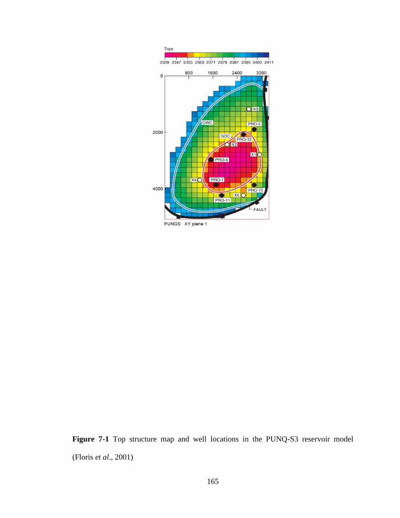
165
Figure 7-1 Top structure map and well locations in the PUNQ-S3 reservoir model
(Floris et al., 2001)
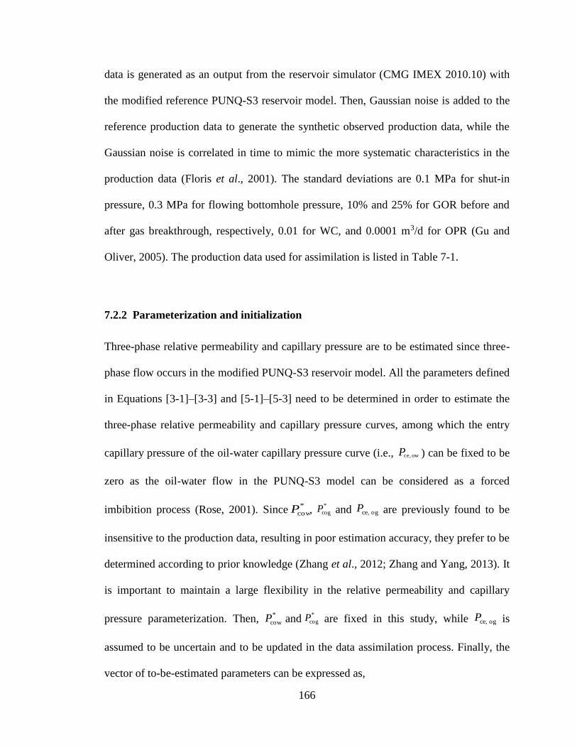
166
data is generated as an output from the reservoir simulator (CMG IMEX 2010.10) with
the modified reference PUNQ-S3 reservoir model. Then, Gaussian noise is added to the
reference production data to generate the synthetic observed production data, while the
Gaussian noise is correlated in time to mimic the more systematic characteristics in the
production data (Floris et al., 2001). The standard deviations are 0.1 MPa for shut-in
pressure, 0.3 MPa for flowing bottomhole pressure, 10% and 25% for GOR before and
after gas breakthrough, respectively, 0.01 for WC, and 0.0001 m3/d for OPR (Gu and
Oliver, 2005). The production data used for assimilation is listed in Table 7-1.
7.2.2 Parameterization and initialization
Three-phase relative permeability and capillary pressure are to be estimated since three-
phase flow occurs in the modified PUNQ-S3 reservoir model. All the parameters defined
in Equations [3-1]–[3-3] and [5-1]–[5-3] need to be determined in order to estimate the
three-phase relative permeability and capillary pressure curves, among which the entry
capillary pressure of the oil-water capillary pressure curve (i.e., ) can be fixed to be
zero as the oil-water flow in the PUNQ-S3 model can be considered as a forced
imbibition process (Rose, 2001). Since , *
cogP and are previously found to be
insensitive to the production data, resulting in poor estimation accuracy, they prefer to be
determined according to prior knowledge (Zhang et al., 2012; Zhang and Yang, 2013). It
is important to maintain a large flexibility in the relative permeability and capillary
pressure parameterization. Then, and*
cogP are fixed in this study, while is
assumed to be uncertain and to be updated in the data assimilation process. Finally, the
vector of to-be-estimated parameters can be expressed as,
owce,P
*
cowP ogce,P
*
cowP ogce,P

167
Table 7-1 Assimilation time points and data types
Time index
Time points (days)
BHP
GOR
WC
OPR
1
1.01
6
6
6
6
2
91
6
6
6
6
3
182
6
6
6
6
4
274
6
6
6
6
5
366 (Shut-in)
6
-
-
-
6
1461 (Shut-in)
6
-
-
-
7
1642
6
6
6
6
8
1826
6
6
6
6
9
1840 (Shut-in)
6
-
-
-
10
1841
6
6
6
6
11
2008
6
6
6
6
12
2192
6
6
6
6
13
2206 (Shut-in)
6
-
-
-
14
2373
6
6
6
6
15
2557
6
6
6
6
16
2571 (Shut-in)
6
-
-
-
17
2572
6
6
6
6
18
2738
6
6
6
6
19
2922
6
6
6
6
20 2936 (Shut-in) 6 - - -
Total 120 84 84 84

168
orggcogce,cogrogrggorwwicowrowrwwows ,,,,,,,,,,,,,, SSPnnnaaSSnnnaa ogm [7-1]
Subsequently, as for the damped IEnKF technique, an ensemble of Ne sets of initial
relative permeability and capillary pressure curves should be initialized as accurately as
possible according to the prior knowledge. The initialization process for the power-law
representation has been described in Section 3.2.1 in detail, while the ensemble size is
chosen to be 50 (i.e., Ne = 50) in this study (Gu and Oliver, 2005; Li, 2010).
In the CMOST, same parameters as in ms (i.e., Equation [7-1]) are to be estimated,
while each parameter has 25 candidate values. The CMG DECE Optimization is used to
conduct the assisted history matching.
7.3 Results and Discussion
7.3.1 Damped IEnKF
The relative permeability and capillary pressure curves are updated by history matching
the production data from the first 8 years including BHP, GOR, WC, and OPR of each
well. The initial relative permeability and capillary pressure curves of the oil-water
system and the gas-oil system are generated according to the initialization process
mentioned previously as shown in Figure 7-2 and Figure 7-3, respectively. Clearly, there
exist large uncertainty ranges associated with the relative permeability and capillary
pressure curves at the beginning.
Ensembles of initial production profiles of each well are then generated by running
the reservoir simulator with the ensemble of initial reservoir models completed with the
initial relative permeability and capillary pressure curves. For example, ensembles of
169
(a)
(b)
Figure 7-2 The reference and initial (a) Relative permeability curves and (b) Capillary
pressure curves of the oil-water system

170
(a)
(b)
Figure 7-3 The reference and initial (a) Relative permeability curves and (b) Capillary
pressure curves of the gas-oil system

171
initial BHP profiles of Well PRO-1 and initial WC profiles of Well PRO-4 are
respectively plotted in Figure 7-4, while ensembles of initial WC profiles of Well PRO-5
and initial GOR profiles of Well PRO-11 are respectively described in Figure 7-5. In
addition, ensembles of initial GOR profiles of Well PRO-12 and initial OPR profiles of
Well PRO-15 are respectively illustrated in Figure 7-6. As can be seen, the black vertical
line divides the time axis into two regions: the history matching period (0 to 2936 days)
and the prediction period (2937 to 6025 days), while the black circles are the observed
production data used for assimilation. The multiple dark-grey lines denote production
profiles simulated from different initial ensemble members, while the red line denotes
the corresponding reference production profile obtained from the modified reference
PUNQ-S3 reservoir model. From Figure 7-4 to Figure 7-6, it can be seen that the
ensemble of initial reservoir models shows great variation in the simulated production
profiles due to their associated large uncertainty ranges in the initial relative permeability
and capillary pressure curves (see Figure 7-2 and Figure 7-3). Meanwhile, the reference
production profiles are all respectively covered by their corresponding ensembles of
initial production profiles. All the other ensembles of initial production profiles of each
production well have the similar trends as shown in Figure 7-4–Figure 7-6, respectively.
Finally, the relative permeability and capillary pressure curves are updated by
assimilating all of the observed production data as depicted in Figure 7-7 and Figure 7-8,
respectively, where the grey shadows are the ensembles of Ne updated relative
permeability and capillary pressure curves. As can be seen, by assimilating all of the
observed production data, the updated relative permeability and capillary pressure curves
are all approaching their corresponding reference curves, while there exists an excellent
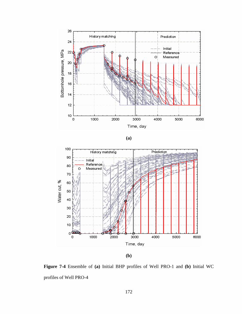
172
(a)
(b)
Figure 7-4 Ensemble of (a) Initial BHP profiles of Well PRO-1 and (b) Initial WC
profiles of Well PRO-4

173
(a)
(b)
Figure 7-5 Ensemble of (a) Initial WC profiles of Well PRO-5 and (b) Initial GOR
profiles of Well PRO-11

174
(a)
(b)
Figure 7-6 Ensemble of (a) Initial GOR profiles of Well PRO-12 and (b) Initial OPR
profiles of Well PRO-15
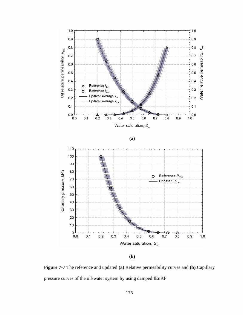
175
(a)
(b)
Figure 7-7 The reference and updated (a) Relative permeability curves and (b) Capillary
pressure curves of the oil-water system by using damped IEnKF
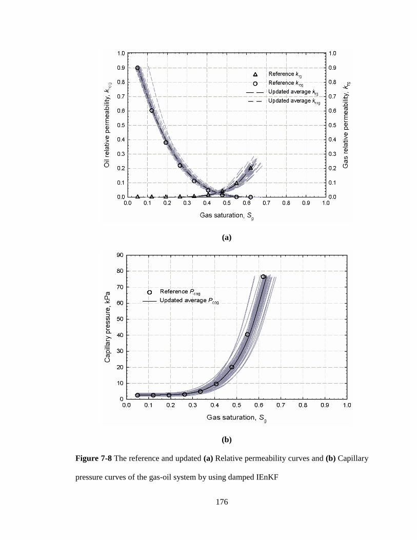
176
(a)
(b)
Figure 7-8 The reference and updated (a) Relative permeability curves and (b) Capillary
pressure curves of the gas-oil system by using damped IEnKF
177
agreement between the updated average relative permeability and capillary pressure
curves and their corresponding reference curves. Meanwhile, the uncertainty ranges
associated with the updated relative permeability and capillary pressure curves are
reduced greatly compared with their initial cases as shown in Figure 7-2 and Figure 7-3.
It can also be seen from Figure 7-8 that the end-point of gas relative permeability
curve (i.e., ag) is overestimated slightly, while there exist larger uncertainty ranges
associated with the updated gas relative permeability curves and gas-oil capillary
pressure curves at a high gas saturation compared with the other updated curves. This
may be ascribed to the fact that production data contains information mainly reflecting a
low gas saturation as the aquifer can provide enough pressure support, resulting in small
gas cap expansion and small solution gas release. It should be noted that production data
can only directly reflect information on the parts of the curves corresponding to the fluid
saturations that exist within the reservoir (Reynolds et al., 2004). Since the power-law
representation model is used to represent the relative permeability and capillary pressure
curves in this study, where the shape of each curve is determined only by the function
index, such as nrog and ncog, it is essentially that relative permeability and capillary
pressure curves at low fluid saturations are accurately evaluated for improving an overall
accuracy. This can explain why good estimation of gas relative permeability curves and
gas-oil capillary pressure curves can still be obtained, even though the production data
only contains the information at a low gas saturation (Reynolds et al., 2004).
Excellent history matching results have been obtained for all production wells,
resulting in accurate prediction of production performance for each well. For example,
the history matching results and production prediction for BHP of Well PRO-1 and WC
178
of Well PRO-4 are respectively plotted in Figure 7-9, while the history matching results
and production prediction for WC of Well PRO-5 and GOR of Well PRO-11 are
respectively illustrated in Figure 7-10. Also, the history matching results and production
prediction for GOR of Well PRO-12 and OPR of Well PRO-15 are shown in Figure 7-11.
In these figures, the grey shadows are the ensembles of the updated production profiles
simulated from the ensemble of the updated reservoir models completed with the
updated relative permeability and capillary pressure curves, while the other symbols
have the same meaning as those in Figure 7-4 – Figure 7-6. Also, the updated reservoir
models generate similar production profiles for each production well as shown in Figure
7-9 – Figure 7-11, respectively.
Obviously, the observed production data of all producers are matched excellently by
the ensemble of the updated reservoir models in the history matching period, while the
predicted production profiles show reasonable spread around the reference cases.
Meanwhile, the uncertainty ranges associated with the updated production profiles are
reduced significantly compared with their corresponding initial cases (see Figure 7-4 –
Figure 7-6), respectively. For example, as for the GOR of Well PRO-12, Figure 7-6a
shows that many of the initial reservoir models produce much more gas than the
reference reservoir model does. However, after assimilating all of the observed
production data, Figure 7-11a indicates that the ensemble of the updated reservoir
models produces almost the same GORs as the reference reservoir model does in the
history matching period.
In the prediction period, Figure 7-11a shows that, although the ensemble of the
updated reservoir models generates certain variations in the predicted GOR profiles for

179
(a)
(b)
Figure 7-9 History matching results and performance prediction of (a) BHP of Well
PRO-1 and (b) WC of Well PRO-4 by using damped IEnKF
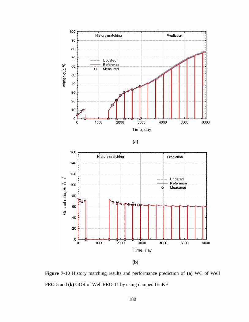
180
(a)
(b)
Figure 7-10 History matching results and performance prediction of (a) WC of Well
PRO-5 and (b) GOR of Well PRO-11 by using damped IEnKF

181
(a)
(b)
Figure 7-11 History matching results and performance prediction of (a) GOR of Well
PRO-12 and (b) OPR of Well PRO-15 by using damped IEnKF
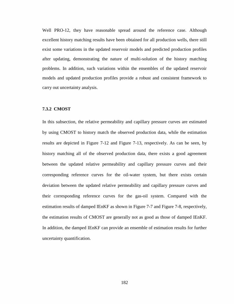
182
Well PRO-12, they have reasonable spread around the reference case. Although
excellent history matching results have been obtained for all production wells, there still
exist some variations in the updated reservoir models and predicted production profiles
after updating, demonstrating the nature of multi-solution of the history matching
problems. In addition, such variations within the ensembles of the updated reservoir
models and updated production profiles provide a robust and consistent framework to
carry out uncertainty analysis.
7.3.2 CMOST
In this subsection, the relative permeability and capillary pressure curves are estimated
by using CMOST to history match the observed production data, while the estimation
results are depicted in Figure 7-12 and Figure 7-13, respectively. As can be seen, by
history matching all of the observed production data, there exists a good agreement
between the updated relative permeability and capillary pressure curves and their
corresponding reference curves for the oil-water system, but there exists certain
deviation between the updated relative permeability and capillary pressure curves and
their corresponding reference curves for the gas-oil system. Compared with the
estimation results of damped IEnKF as shown in Figure 7-7 and Figure 7-8, respectively,
the estimation results of CMOST are generally not as good as those of damped IEnKF.
In addition, the damped IEnKF can provide an ensemble of estimation results for further
uncertainty quantification.
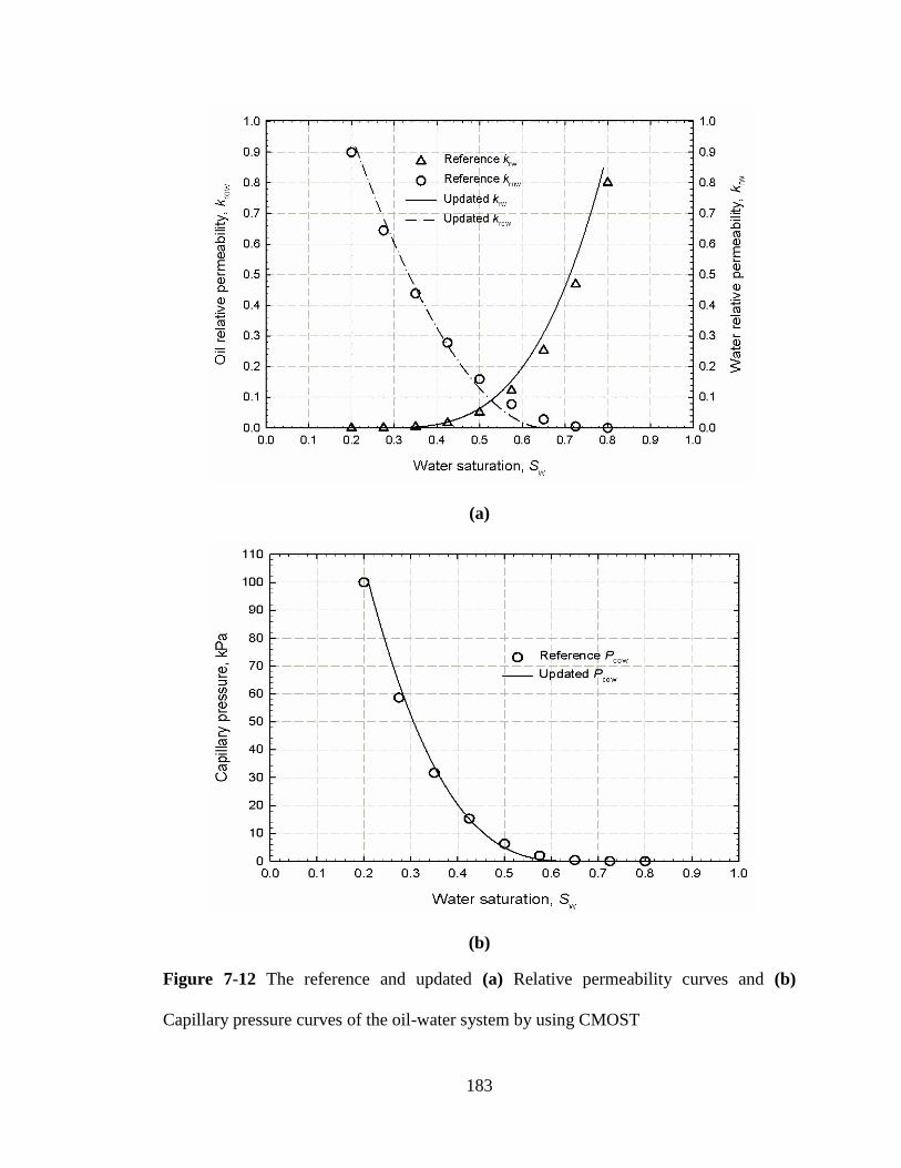
183
(a)
(b)
Figure 7-12 The reference and updated (a) Relative permeability curves and (b)
Capillary pressure curves of the oil-water system by using CMOST

184
(a)
(b)
Figure 7-13 The reference and updated (a) Relative permeability curves and (b)
Capillary pressure curves of the gas-oil system by using CMOST

185
Reasonable good history matching results have been obtained for all production wells
by using CMOST. However, compared with the damped IEnKF technique, the less
accurate estimation results of relative permeability and capillary pressure curves by
using CMOST result in less accurate prediction of production performance for
production wells. For example, the comparison between both the history matching
results and production prediction performance of CMOST and those of damped IEnKF
for the selected wells are respectively illustrated in Figure 7-14 – Figure 7-16. As can be
seen, in the history matching period, the damped IEnKF and CMOST generate similar
good history matching results, though the CMOST estimates the relative permeability
and capillary pressure curves less accurately than the damped IEnKF. Also, this further
demonstrates the nature of multi-solution of history matching problems. However, the
less estimation accuracy of the CMOST results in larger deviation in the prediction
period compared with the damped IEnKF technique. Furthermore, it is indicated that a
history matched reservoir model may not predict future production accurately due to the
nature of multi-solution of history matching problems. Therefore, in order to obtain
reliable production prediction, the reservoir parameters have to be determined accurately
by using reliable estimation techniques.
7.4 Summary
The damped IEnKF algorithm has been successfully applied to simultaneously estimate
relative permeability and capillary pressure for the PUNQ-S3 reservoir model by
assimilating long-term field production data. In addition, the performance of the damped
IEnKF algorithm has been compared with that of CMOST. As for the damped IEnKF

186
(a)
(b)
Figure 7-14 Comparison of history matching results and performance prediction for (a)
BHP of Well PRO-1 and (b) WC of Well PRO-4 by using damped IEnKF and CMOST
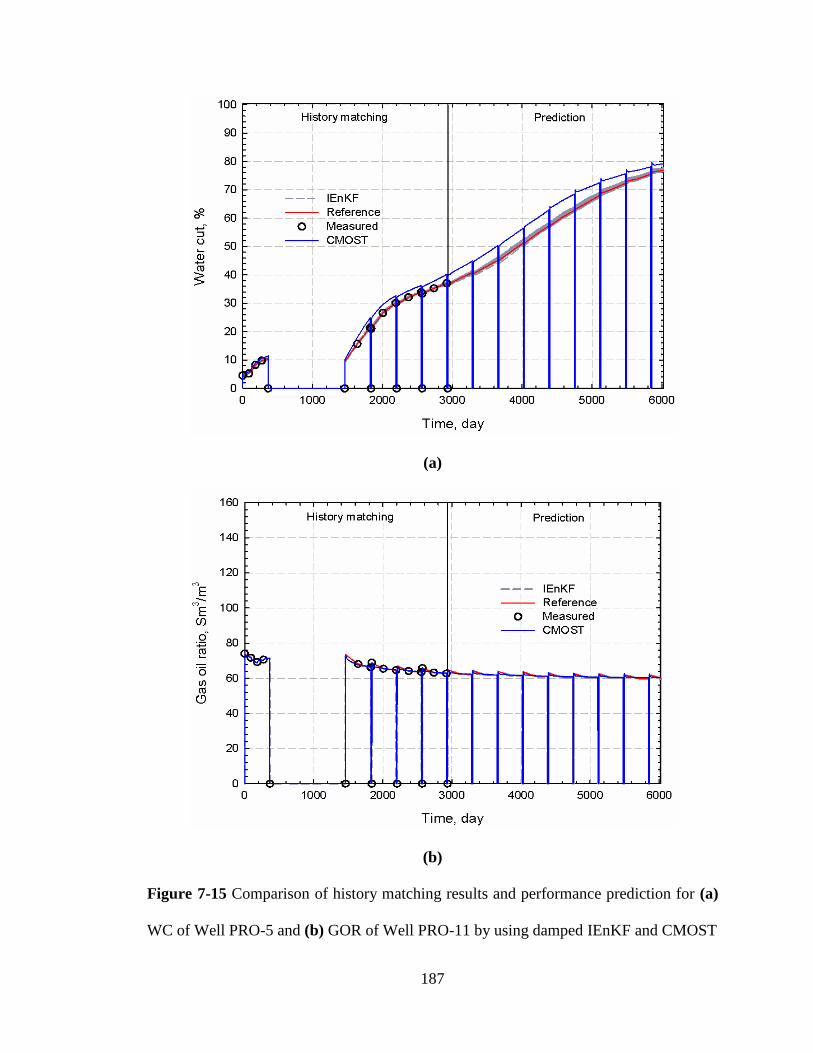
187
(a)
(b)
Figure 7-15 Comparison of history matching results and performance prediction for (a)
WC of Well PRO-5 and (b) GOR of Well PRO-11 by using damped IEnKF and CMOST

188
(a)
(b)
Figure 7-16 Comparison of history matching results and performance prediction for (a)
GOR of Well PRO-12 and (b) OPR of Well PRO-15 by using damped IEnKF and
CMOST

189
algorithm, at the beginning, the initial relative permeability and capillary pressure curves
are associated with large uncertainty ranges, resulting in great variations in the simulated
production profiles in both history matching and prediction periods. Finally, these
parameters are updated by assimilating all of the observed production data to achieve an
excellent agreement with their corresponding reference curves, while their uncertainty
ranges are reduced significantly compared with their corresponding initial cases.
Although ag is overestimated slightly and there still exist larger uncertainty ranges
associated with the updated gas relative permeability and gas-oil capillary pressure
curves at a higher gas saturation compared with the other updated curves, excellent
history matching results have been obtained. Also, the production prediction from the
ensemble of the updated reservoir models has a reasonable spread around the reference
cases. The uncertainty ranges, especially associated with the updated gas relative
permeability and gas-oil capillary pressure curves, may be further mitigated at a later
time by assimilating more production data. The CMOST estimates the relative
permeability and capillary pressure less accurately than the damped IEnKF, but both
damped IEnKF and CMOST generate similar good history matching results due to the
nature of multi-solution of history matching problems. However, the CMOST predicts
future production with larger deviations compared with the damped IEnKF technique
due to its less estimation accuracy. Therefore, in order to obtain reliable production
prediction, reliable techniques are needed to carry out history matching.

190
CHAPTER 8 CONCLUSIONS AND RECOMMENDATIONS
8.1 Conclusions
The major contributions of this dissertation can be summarized as follows:
(1). An ensemble-based history matching technique using the confirming EnKF
algorithm together with its detailed workflow have been developed to evaluate
relative permeability and capillary pressure for hydrocarbon reservoirs by
assimilating available measurement data. This newly developed technique has
been validated and applied to simultaneously evaluate relative permeability and
capillary pressure curves in both conventional reservoirs and tight formations.
(2). To improve the performance of the confirming EnKF algorithm, a new form of
damped IEnKF algorithm has been proposed and applied to simultaneously
evaluate relative permeability and capillary pressure curves for a tight formation
from the laboratory coreflooding experiment where only cumulative oil
production and pressure drop are available to be assimilated.
(3). The newly developed damped IEnKF algorithm has been successfully applied to
simultaneously evaluate three-phase relative permeability and capillary pressure
curves for the 3D PUNQ-S3 reservoir model, which is a standard synthetic test
case that is based on a real field, by assimilating long-term field production data.
As for the aforementioned techniques, the major conclusions can be drawn as follows:
(1). The relative permeability and capillary pressure curves can be represented by
using the power-law model and/or B-spline model whose parameters are to be

191
tuned automatically and finally determined once the measurement data has been
history matched. The B-spline model has been proven to represent the relative
permeability and capillary pressure curves more flexibly, whereas the power-law
model has fewer coefficients to be estimated during the history matching process.
(2). In general, the relative permeability and capillary pressure curves are updated
progressively and their uncertainties are reduced gradually as more measurement
data are assimilated. Accordingly, the uncertainty ranges associated with the
updated production profiles are all reduced greatly due to the significantly
reduced uncertainties in the updated relative permeability and capillary pressure
curves. In addition, the relative permeability is found to be estimated more
accurately than the capillary pressure owing to its more sensitive to the
measurement data.
(3). As for the numerical coreflooding experiments, no matter with or without fluid
saturation profile available to be assimilated, there exists an excellent agreement
between the updated and reference relative permeability and capillary pressure
curves, resulting in excellent history matching results. In the laboratory
coreflooding experiments, however, the estimation and history matching results
with fluid saturation profiles available to be assimilated are better than those
without fluid saturation profiles available to be assimilated.
(4). As for the laboratory coreflooding experiment with oil saturation profile available
to be assimilated, the relative permeability and capillary pressure curves are
finally determined by using the confirming EnKF algorithm to assimilate all of
the measurement data. Although there is a minor mismatch for the oil saturation

192
profile, there exists a good agreement between the measured and simulated
pressure drop and cumulative water production.
(5). As for the laboratory coreflooding experiment without saturation profile available
to be assimilated, the relative permeability and capillary pressure curves are
finally determined by using the confirming EnKF algorithm to assimilate the
conventional measurement data, i.e., including only cumulative oil production
and pressure drop. A reasonable good history matching has been obtained for the
pressure drop, but there exists certain mismatch for the history matching result of
cumulative oil production due to the strong nonlinearity of the whole data
assimilation system where the developed confirming EnKF algorithm may not
function well.
(6). As for the synthetic 2D reservoir model, the relative permeability and capillary
pressure curves can be simultaneously estimated by using the confirming EnKF
algorithm to history match the field production data. The two-phase relative
permeability and capillary pressure curves can be determined accurately, leading
to excellent history matching results. Although there exists a good agreement
between the updated and reference relative permeability and capillary pressure
curves together with good history matching results in the three-phase flow, the
estimation accuracy is compromised compared to that of the two-phase flow.
(7). The damped IEnKF algorithm has performed better than the confirming EnKF
algorithm in the laboratory coreflooding experiment where only cumulative oil
production and pressure drop are available to be assimilated. Not only can the
relative permeability and capillary pressure curves be simultaneously determined
193
by assimilating the available measurement data, but also there exist much better
history matching results than those of the confirming EnKF algorithm. It has
been proven that the damped IEnKF algorithm can function well in the strongly
nonlinear data assimilation system where the traditional and confirming EnKF
algorithms may find their limitations.
(8). The damped IEnKF algorithm can function well in the large-scale history
matching problems, which has been proven by using the PUNQ-S3 reservoir
model. The three-phase relative permeability and capillary pressure curves have
been determined accurately by using the damped IEnKF algorithm to assimilate
the long-term field production data, leading to excellent history matching results.
Although excellent history matching results have been obtained, there still exist
some variations in the updated reservoir models and predicted production profiles.
Although both the damped IEnKF and CMOST generate similar good history
matching results, the estimation results and production prediction performance of
the CMOST are generally not as good as those of the damped IEnKF.
In a word, the newly developed ensemble-based history matching techniques have
been proven to be able to simultaneously evaluate relative permeability and capillary
pressure for hydrocarbon reservoirs, while they are easy to be implemented. In addition,
the ensemble-based history matching techniques can provide an ensemble of history-
matched reservoir models which are suitable for uncertainty analysis under a unified and
consistent framework.
194
8.2 Recommendations
The following are recommendations for future work:
(1). Applications of the new damped IEnKF technique need to be extended to various
real field cases. For example, the Norne Field is an offshore oilfield, Norway, that
has been put in production as a subsea field mainly through water injection since
1997, which has been recently used as a benchmark case for testing history
matching technologies (Chen and Oliver, 2013).
(2). The reservoir models need to be calibrated by using the observations from well
testing, well logging, tracer and/or seismic data. For example, the damped IEnKF
technique can be applied to improve the reservoir characterization by assimilating
the history production data together with the tracer analysis and/or 4D seismic
data, while appropriate localization technique needs to be developed.
(3). More studies are needed to improve the stability, reliability and efficiency of the
ensemble-based history matching techniques. For example, more advanced
techniques are needed to prevent ensemble collapse issues for the ensemble-
based history matching technologies (Sarma and Chen, 2013), while the
ensemble smoother (ES) algorithm has shown great potential to improve the
history matching efficiency significantly (Skjervheim et al., 2011; Chen and
Oliver, 2012).
(4). Efforts are needed to integrate the assisted history matching with the reservoir
production optimization techniques through a loop to fulfill the concept of
closed-loop reservoir management. The EnKF and other related ensemble-based
algorithms are well suitable for assisted history matching in the closed-loop

195
reservoir management (Peters et al., 2013), while the EnKF can also be applied
for reservoir production optimization.

196
REFERENCES
Aanonsen, S.I.; Nævdal, G.; Oliver, D.S.; Reynolds, A.C.; and Valles, B. The Ensemble
Kalman Filter in Reservoir Engineering-A Review. SPE Journal 2009, 14(3),
393–412.
Abadpour, A.; Bergey, P.; and Piasecki, R. 4D Seismic History Matching with Ensemble
Kalman Filter-Assimilation on Hausdorff Distance to Saturation Front. Paper
SPE 163635, presented at the SPE Reservoir Simulation Symposium, Woodlands,
TX, February 18–20, 2013.
Agbalaka, C.C. and Oliver, D.S. Application of the EnKF and Localization to Automatic
History Matching of Facies Distribution and Production Data. Mathematical
Geosciences 2008, 40(4), 353–374.
Angeles, R.; Torres-Verdín, C.; Hadibeik, A.; and Sepehrnoori, K. Estimation of
Capillary Pressure and Relative Permeability from Formation-tester
Measurements Using Design of Experiment and Data-weighing Inversion:
Synthetic and Field Examples. Journal of Petroleum Science and Engineering
2010, 75(1–2), 19–32.
Annan, J.D.; Lunt, D.J.; Hargreaves, J.C.; and Valdes, P.J. Parameter Estimation in An
Atmospheric GCM Using the Ensemble Kalman Filter. Nonlinear Processes in
Geophysics 2007, 12(3), 363–371.
Barrera, A. History Matching by Simultaneous Calibration of Flow Functions. PhD
Dissertation, University of Texas at Austin, Austin, TX, USA, 2007.
Blunt, M.J. Flow in Porous Media−Pore-network Models and Multiphase Flow. Current
Opinion in Colloid & Interface Science 2001, 6(3), 197–207.
197
Cancelliere, M.; Viberti, D.; and Verga, F. Assisted History Matching for Petroleum
Reservoirs in the Social Computing Era. American Journal of Applied Sciences
2013, 10(8), 901–916.
Chardaire-Riviere, C.; Chavent, G.; Jaffre, J.; Liu, J.; and Bourblaux, B.J. Simultaneous
Estimation of Relative Permeability and Capillary Pressure. SPE Formation
Evaluation 1992, 7(4), 283–289.
Chavent, G.; Cohen, G.; and Espy, M. Determination of Relative Permeability and
Capillary Pressure by An Automatic Adjustment Method. Paper SPE 9237,
presented at the SPE Annual Technical Conference and Exhibition, Dallas, TX,
September 21–24, 1980.
Chavent, G.; Dupuy, M.; and Lemonnier, P. History Matching by Use of Optimal Theory.
SPE Journal 1975, 15(1), 74–86.
Chen, S.; Li, H.; Yang, D.; and Tontiwachwuthikul, P. An Efficient Methodology of
Performance Optimization and Uncertainty Analysis in CO2 EOR Processes.
Petroleum Science and Technology 2012, 30(12), 1195–1209.
Chen, S.; Li, G.; Peres, A.; and Reynolds, A.C. A Well Test for In-situ Determination of
Relative Permeability Curves. SPE Reservoir Evaluation & Engineering 2008,
11(1), 95–107.
Chen, W.H.; Gavalas, G.R.; Seinfeld, J.H.; and Wasserman, M.L. A New Algorithm for
Automatic History Matching. SPE Journal 1974, 14(6), 593–608.
Chen, Y. and Oliver, D.S. Localization of Ensemble-based Control Setting Updates for
Production Optimization. Paper SPE 125042, presented at the SPE Annual
Technical Conference and Exhibition, New Orleans, LA, October 4–7, 2009.

198
Chen, Y. and Oliver, D.S. Ensemble-based Closed-loop Optimization Applied to Brugge
Field. SPE Reservoir Evaluation & Engineering 2010a, 13(1), 56–71.
Chen, Y. and Oliver, D.S. Cross-covariances and Localization for EnKF in Multiphase
Flow Data Assimilation. Computational Geosciences 2010b, 14(4), 579–601.
Chen, Y. and Oliver, D.S. Parameterization Techniques to Improve Mass Conservation
and Data Assimilation for Ensemble Kalman Filter. Paper SPE 133560, presented
at the SPE Western Regional Meeting, Anaheim, CA, May 27–29, 2010c.
Chen, Y. and Oliver, D.S. Ensemble Randomized Maximum Likelihood Method as An
Iterative Ensemble Smoother. Mathematical Geosciences 2012, 44(1), 1–26.
Chen, Y. and Oliver, D.S. History Matching of the Norne Full Field Model Using An
Iterative Ensemble Smoother. Paper SPE 164902, presented at the 75th EAGE
Conference & Exhibition incorporating SPE EUROPE, London, United Kingdom,
June 10–13, 2013.
Chen, Y.; Oliver, D.S.; and Zhang, D.X. Efficient Ensemble-based Closed-loop
Production Optimization. SPE Journal 2009a, 14(4), 634–645.
Chen, Y.; Oliver, D.S.; and Zhang, D.X. Data Assimilation for Nonlinear Problems by
Ensemble Kalman Filter with Reparameterization. Journal of Petroleum Science
and Engineering 2009b, 66(1–2), 1–14.
Computer Modelling Group Ltd. User’s Guide. CMOST Studio 2010.
Deutsch, C.V. and Journel, A.G. The Application of Simulated Annealing to Stochastic
Reservoir Modeling. SPE Advanced Technology Series 1994, 2(2), 222–227.
Donaldson, E.C.; Chilingarian, G.V.; and Yen, T.F. Enhanced Oil Recovery:
Fundamentals and Analysis, Vol. 1. Elsevier, New York, 1985.

199
Dong, Y.; Gu, Y.; and Oliver, D.S. Sequential Assimilation of 4D Seismic Data for
Reservoir Description Using the Ensemble Kalman Filter. Journal of Petroleum
Science and Engineering 2006, 53(1), 83–99.
Dong, Y. and Oliver, D.S. Quantitative Use of 4D Seismic Data for Reservoir
Description. SPE Journal 2005, 10(1), 91–99.
Emerick, A.A. and Reynolds, A.C. History Matching Time-lapse Seismic Data Using the
Ensemble Kalman Filter with Multiple Data Assimilations. Computers &
Geosciences 2012, 16, 639–659.
Emerick, A.A. and Reynolds, A.C. History-matching Production and Seismic Data in A
Real Field Using the Ensemble Smoother with Multiple Data Assimilation. Paper
SPE 163675, presented at the SPE Reservoir Simulation Symposium, Woodlands,
TX, February 18–20, 2013.
Erbas, D. and Christie, M.A. Effect of Sampling Strategies on Prediction Uncertainty
Estimation. Paper SPE 106229, presented at the SPE Reservoir Simulation
Symposium, Houston, TX, February 26–28, 2007.
Evensen, G. Data Assimilation: The Ensembles Kalman Filter. Springer, Berlin, 2006.
Evensen, G. The Ensemble Kalman Filter for Combined State and Parameter Estimation.
Control Systems, IEEE 2009, 29(3), 83–104.
Evensen, G.; Hove, J.; Meisingset, H.C.; Reiso, E.; Seim, K.S.; and Espelid, Ø. Using
the EnKF for Assisted History Matching of a North Sea Reservoir Model. Paper
SPE 106184, presented at the SPE Reservoir Simulation Symposium, Woodlands,
TX, February 26–28, 2007.

200
Eydinov, D.; Gao, G.; Li, G.; and Reynolds, A.C. Simultaneous Estimation of Relative
Permeability and Porosity/Permeability Fields by History Matching Production
Data. Journal of Canadian Petroleum Technology 2009, 48(12), 13–25.
Fallgren, M. On the Robustness of Conjugate-gradient Methods and Quasi-Newton
Methods. Master Thesis, Royal Institute of Technology, Stockholm, Sweden,
2006.
Farmer, C.L. The Mathematical Generation of Reservoir Geology. Oxford University
Press, New York, 1991.
Firoozabadi, A. and Aziz, K. Relative Permeabilities from Centrifuge Data. Journal of
Canadian Petroleum Technology 1991, 30(5), 33–42.
Fletcher, R. Practical Methods of Optimization (2nd Ed.). Wiley, New York, 1987.
Floris, F.J.T.; Bush, M.D.; Cuypers, M.; Roggero, F.; and Syversveen, A-R. Methods for
Quantifying the Uncertainty of Production Forecasts: A Comparative Study.
Petroleum Geoscience 2001, 7(S), S87–S96.
Gao, G. and Reynolds, A.C. An Improved Implementation of the LBFGS Algorithm for
Automatic History Matching. SPE Journal 2006, 11(1), 5–17.
Gervais, V. and Roggero, F. Integration of Saturation Data in a History Matching
Process Based on Adaptive Local Parameterization. Journal of Petroleum Science
and Engineering 2010, 73(1–2), 86–98.
Goda, H.M. and Behrenbruch, P. Using a Modified Brooks-Corey Model to Study Oil-
Water Relative Permeability for Diverse Pore Structures. Paper SPE 88538,
presented at the SPE Asia Pacific Oil and Gas Conference and Exhibition, Perth,
Australia, October 18–20, 2004.

201
Goldberg, D.E. Genetic Algorithms in Search, Optimization, and Machine Learning.
Addison-Wesley, Boston, 1989.
Gu, Y. and Oliver, D.S. History Matching of the PUNQ-S3 Reservoir Model Using the
Ensemble Kalman Filter. SPE Journal 2005, 10(2), 217–224.
Gu, Y. and Oliver, D.S. An Iterative Ensemble Kalman Filter for Multiphase Fluid Flow
Data Assimilation. SPE Journal 2007, 12(4), 438–446.
Han, M.; Li, G.; and Chen, J. Assimilating Microseismic and Welltest Data Using EnKF
for Accurate Reservoir Characterisation. Paper SPE 16725, presented at the 6th
International Petroleum Technology Conference, Beijing, China, March 26–28,
2013.
Haugen, V.; Nævdal, G.; Natvik, L.J.; Evensen, G.; Berg, A.M.; and Flornes, K.M.
History Matching Using the Ensemble Kalman Filter on a North Sea Field Case.
SPE Journal 2008, 13(4), 382–391.
He, N.; Reynolds, A.C.; and Oliver, D.S. Three-dimensional Reservoir Description from
Multiwell Pressure Data and Prior Information. SPE Journal 1997, 2(3), 312–327.
Honarpour, M. and Mahmood, S.M. Relative-permeability Measurements: An Overview.
Journal of Petroleum Technology 1988, 40(8), 963–966.
Houtekamer, P.L. and Mitchell, H.L. Data Assimilation Using an Ensemble Kalman
Filter Technique. Monthly Weather Review 1998, 126(3), 796–811.
Iwere, F.O.; Heim, R.N.; and Cherian, B.V. Numerical Simulation of Enhanced Oil
Recovery in the Middle Bakken and Upper Three Forks Tight Oil Reservoirs of
the Williston Basin. Paper SPE 154937, presented at the SPE Americas
Unconventional Resources Conferences, Pittsburgh, PA, June 5–7, 2012.
202
Jafarpour, B. and McLaughlin, D.B. Efficient Permeability Parameterization with the
Discrete Cosine Transform. Paper SPE 106453, presented at the SPE Reservoir
Simulation Symposium, Houston, TX, February 26–28, 2007a.
Jafarpour, B. and McLaughlin, D.B. History Matching with an Ensemble Kalman Filter
and Discrete Cosine Parameterization. Paper SPE 108761, presented at the SPE
Annual Technical Conference and Exhibition, Anaheim, CA, November 11–14,
2007b.
Jazwinski, A.H. Stochastic Processes and Filtering Theory, Mathematics in Science and
Engineering, Vol. 64. Academic Press, New York, 1970.
Kamath, J.; Nakagawa, F.; Meyer, R.; Kabir, S.; and Hobbet, R. Laboratory Evaluation
of Waterflood Residual Oil Saturation in Four Carbonate Cores. Paper SCA 2001,
SCA Symposium Technical Programme, 12, 1–13.
Kameswaran, S.; Biegler, L.T.; and Staus, G.H. Dynamic Optimization for the Core-
flooding Problem in Reservoir Engineering. Computers & Chemical Engineering
2005, 29(8), 1787–1800.
Kerig, P.D. and Watson, A.T. A New Algorithm for Estimating Relative Permeabilities
from Displacement Experiments. SPE Reservoir Engineering 1987, 2(1), 103–
112.
Krymskaya, M.V.; Hanea, R.G.; and Verlaan, M. An Iterative Ensemble Kalman Filter
for Reservoir Engineering Applications. Computers & Geosciences 2009, 13,
235–244.
Kulkarni, K.N. and Datta-Gupta, A. Estimating Relative Permeability from Production
Data: A Streamline Approach. SPE Journal 2000, 5(4), 402–411.
203
Kulkarni, R.N.; Watson, A.T.; Nordtvedt, J.E.; Brancolini, A.; and Johnsen, O.
Estimation of Multiphase Flow Functions from Dynamic Displacement Data:
Applications of NMR Imaging. Paper SPE 36855, presented at the SPE European
Petroleum Conference, Milan, Italy, October 22–24, 1996.
Kulkarni, R.N.; Watson, A.T.; and Nordtvedt, J.E. Estimation of Porous Media Flow
Functions Using NMR Imaging Data. Magnetic Resonance Imaging 1998, 16(5–
6), 707–709.
Lampton, M. Damping-undamping Strategies for the Levenberg-Marquardt Nonlinear
Least-squares Method. Computers in Physics 1997, 11(1), 110–115.
Lee, T.Y.; Kravaris, C.; and Seinfeld, J.H. History Matching by Spline Approximation
and Regularization in Single-phase Areal Reservoirs. SPE Reservoir Engineering
1986, 1(5), 521–534.
Lee, T.Y. and Seinfeld, J.H. Estimation of Two-phase Petroleum Reservoir Properties by
Regularization. Journal of Computational Physics 1987, 69(2), 397–419.
Li, G. and Reynolds, A.C. Iterative Ensemble Kalman Filters for Data Assimilation. SPE
Journal 2009, 14(3), 496–505.
Li, H. Ensemble-based History Matching and Its Application in Estimating Reservoir
Petrophysical Properties. PhD Dissertation, University of Regina, Regina, SK,
Canada, 2010.
Li, H.; Chen, S.; Yang, D.; and Tontiwachwuthikul, P. Ensemble-based Relative
Permeability Estimation Using B-spline Model. Transport in Porous Media
2010a, 85(3), 703–721.
204
Li, H.; Chen, S.; Yang, D.; and Tontiwachwuthikul, P. Estimation of Relative
Permeability by Assisted History Matching Using the Ensemble Kalman Filter
Method. Journal of Canadian Petroleum Technology 2012, 51(3), 205–214.
Li, H. and Yang, D. Estimation of Multiple Petrophysical Parameters for Hydrocarbon
Reservoirs with the Ensemble-based Technique. Advances in Petroleum
Exploration and Development 2012, 4(2), 1–17.
Li, H.; Yang, D.; and Arhuoma, M. Relative Permeability Estimation from Displacement
Experiments Using EnKF Method. Paper SPE 131633, presented at the CPS/SPE
International Oil and Gas Conference and Exhibition, Beijing, China, June 8–10,
2010b.
Li, K. and Horne, R.N. An Experimental and Analytical Study of Steam/Water Capillary
Pressure. SPE Reservoir Evaluation & Engineering 2001, 4(6), 477–482.
Li, K. and Horne, R.N. Comparison of Methods to Calculate Relative Permeability from
Capillary Pressure in Consolidated Water-wet Porous Media. Water Resources
Research 2006, 42(6), 1–9.
Li, R.; Reynolds, A.C.; and Oliver, D.S. History Matching of Three-phase Flow
Production Data. SPE Journal 2003, 8(4), 328–340.
Liang, B. An Ensemble Kalman Filter Module for Automatic History Matching. PhD
Dissertation, University of Texas at Austin, Austin, TX, USA, 2007.
Liu, N. and Oliver, D.S. Automatic History Matching of Geologic Facies. SPE Journal
2004, 9(4), 188–195.

205
Liu, N. and Oliver, D.S. Critical Evaluation of the Ensemble Kalman Filter on History
Matching of Geologic Facies. SPE Reservoir Evaluation & Engineering 2005,
8(6), 470–477.
Liu, R.; Liu, H.; Li, X.; Wang, J.; and Pang, C. Calculation of Oil and Water Relative
Permeability for Extra Low Permeability Reservoir. Paper SPE 131388,
presented at the CPS/SPE International Oil & Gas Conference and Exhibition,
Beijing, China, June 8–10, 2010.
Lohne, A. and Virnovsky, G. Three-phase Upscalling in Capillary and Viscous Limit.
Paper SPE 99567, presented at the SPE/DOE Symposium on Improved Oil
Recovery, Tulsa, OK, April 22–26, 2006.
Lorentzen, R.J.; Fjelde, K.K.; Frφyen, J.; Lage, A.C.V.M.; Nævdal, G.; and Vefring, E.H.
Underbalanced Drilling: Real Time Data Interpretation and Decision Support.
Paper SPE 67693, presented at the SPE/IADC Drilling Conference, Amsterdam,
Netherlands, February 27–March 1, 2001.
Lorentzen, R.J. and Nævdal, G. An Iterative Ensemble Kalman Filter. Automatic Control,
IEEE Transactions 2011, 56(8), 1990–1995.
Lorentzen, R.J.; Nævdal, G.; and Shafieirad, A. Estimating Facies Fields by Use of the
Ensemble Kalman Filter and Distance Functions-Applied to Shallow-Marine
Environments. SPE Journal 2013, 18(1), 146–158.
Makhlouf, E.M.; Chen, W.H.; Wasserman, M.L.; and Seinfeld, J.H. A General History
Matching Algorithm for Three-phase, Three-dimensional Petroleum Reservoirs.
SPE Advanced Technology Series 1993, 1(2), 83–92.
206
Manrique, E.; Muci, V.E.; and Gurfinkel, M.E. EOR Field Experiences in Carbonate
Reservoirs in the United States. SPE Reservoir Evaluation & Engineering 2007,
10(6), 667–686.
Manrique, E.; Thomas, C.; Ravikiran, R.; Izadi, M.; Lantz, M.; Romero, J.; and Alvarado,
V. EOR: Current Status and Opportunities. Paper SPE 130113, presented at the
SPE Improved Oil Recovery Symposium, Tulsa, OK, April 24–28, 2010.
Maschio, C. and Schiozer, D.J. Development and Application of Methodology for
Assisted History Matching. Paper SPE 94882, presented at the SPE Latin
American and Caribbean Petroleum Engineering Conference, Rio de Janeiro,
Brazil, June 20–23, 2005.
Mejia, G.M.; Watson, A.T.; and Nordtvedt, J.E. Estimation of Three-phase Flow
Functions in Porous Media. AIChE Journal 1996, 42(7), 1957–1967.
Metropolis, N.; Rosenbluth, A.W.; Rosenbluth, M.N.; Teller, A.H.; and Teller, E.
Equation of State Calculations by Fast Computing Machines. Journal of
Chemical Physics 1953, 21(6), 1087–1092.
Nævdal, G.; Brouwer, D.R.; and Jansen, J.D. Water-flooding Using Closed-loop Control.
Computational Geosciences 2006, 10(1), 37–60.
Nævdal, G.; Johnsen, L.M.; Aanonsen, S.I.; and Vefring, E.H. Reservoir Monitoring and
Continuous Model Updating Using Ensemble Kalman Filter. SPE Journal 2005,
10(1), 66–74.
Nævdal, G.; Mannseth, T.; and Vefring, E.H. Near-well Reservoir Monitoring through
Ensemble Kalman Filter. Paper SPE 75235, presented at the SPE/DOE Improved
Oil Recovery Symposium, Tulsa, OK, April 13–17, 2002.

207
Nejadi, S.; Leung, J.; and Trivedi, J.J. Integration of Production Data for Estimation of
Natural Fracture Properties in Tight Gas Reservoirs Using Ensemble Kalman
Filter. Paper SPE 162783, presented at the SPE Canadian Unconventional
Resources Conference, Calgary, AB, October 30– November 1, 2012.
Nieto, V.L.; Savioli, G.B.; and Bidner, M.S. On the Inverse Problem of the Estimation of
Multiphase Flow Functions. Paper SPE 92007, presented at the SPE International
Petroleum Conference, Puebla, Mexico, November 8–9, 2004.
Nocedal, J. and Wright, S.J. Numerical Optimization. Springer-Verlag, New York, 1999.
Oliver, D.S. and Chen, Y. Recent Progress on Reservoir History Matching: A Review.
Computational Geosciences 2011, 15(1), 185–221.
Oliver, D.; Cunha, L.; and Reynolds, A. Markov Chain Monte Carlo Methods for
Conditioning a Permeability Field to Pressure Data. Mathematical Geology 1997,
29(1), 61–91.
Oliver, D.S.; Reynolds, A.C.; and Liu, N. Inverse Theory for Petroleum Reservoir
Characterization and History Matching. Cambridge University Press, Cambridge,
2008.
Ouenes, A. and Bhagavan, S. Application of Simulated Annealing and Other Global
Optimization Method to Reservoir Description: Myths and Realities. Paper SPE
28415, presented at the SPE Annual Technical Conference and Exhibition, New
Orleans, LA, September 25–28, 1994.
Ouenes, A.; Bréfort, B.; Meunier, G.; and Dupéré, S. A New Algorithm for Automatic
History Matching: Application of Simulated Annealing Method (SAM) to
Reservoir Inverse Modeling. Paper SPE 26297, Unsolicited, 1993.

208
Panwar, A.; Trivedi, J.J.; and Nejadi, S. Importance of Distributed Temperature Sensor
(DTS) Placement for SAGD Reservoir Characterization and History Matching
within Ensemble Kalman Filter (EnKF) Framework. Paper SPE 153659,
presented at the SPE Latin America and Caribbean Petroleum Engineering
Conference, Mexico City, Mexico, April 16–18, 2012.
Peters, E.; Chen, Y.; Leeuwenburgh, O.; and Oliver, D.S. Extended Brugge Benchmark
Case for History Matching and Water Flooding Optimization. Computers &
Geosciences 2013, 50, 16–24.
Pickup, G.E.; Stephen, K.D.; Ma, J.; Zhang, P.; and Clark, J.D. Multi-stage Upscaling:
Selection of Suitable Methods. Transport in Porous Media 2005, 58(1–2), 191–
216.
Portellaand, R.C.M. and Prais, F. Use of Automatic History Matching and Geostatistical
Simulation to Improve Production Forecast. Paper SPE 53976, presented at the
SPE Latin American and Caribbean Petroleum Engineering Conference, Caracas,
Venezuela, April 21–23, 1999.
Qin, J. Variation of the Permeability of the Low-permeability Sandstone Reservoir under
Variable Confined Pressure. Journal of Xi’an Petroleum Institute 2002, 17(4),
28–35.
Reynolds, A.C.; He, N.; Chu, L.; and Oliver, D.S. Reparameterization Techniques for
Generating Reservoir Descriptions Conditioned to Variograms and Well-test
Pressure Data. SPE Journal 1996, 1(4), 413–426.

209
Reynolds, A.C.; Li, R.; and Oliver, D.S. Simultaneous Estimation of Absolute and
Relative Permeability by Automatic History Matching of Three-phase Flow
Production Data. Journal of Canadian Petroleum Technology 2004, 43(3), 37–46.
Reynolds, A.C.; Zafari, M.; and Li, G. Iterative Forms of the Ensemble Kalman Filter.
Paper A030, presented at the 10th European Conference on the Mathematics of
Oil Recovery, Amsterdam, Netherlands, September 4–7, 2006.
Richmond, P.C. and Watson, A.T. Estimation of Multiphase Flow Functions from
Displacement Experiments. SPE Reservoir Engineering 1990, 5(1), 121–127.
Rodrigues, J.R.P. Calculating Derivatives for History Matching in Reservoir Simulators.
Paper SPE 93445, presented at the SPE Reservoir Simulation Symposium,
Woodlands, TX, January 31–February 2, 2005.
Rodrigues, J.R.P.; Wachter, A.; Conn, A.; de Moraes, R.J.; and da Silva, F.P.T.
Combining Adjoint Calculations and Quasi-Newton Methods for Automatic
History Matching. Paper SPE 99996, presented at the SPE Europec/EAGE
Annual Conference and Exhibition, Vienna, Austria, June12–15, 2006.
Romero, C.E. and Carter, J.N. Using Genetic Algorithms for Reservoir Characterisation.
Journal of Petroleum Science and Engineering 2001, 31(2–4), 113–123.
Rose, W. Modeling Forced versus Spontaneous Capillary Imbibition Processes
Commonly Occurring in Porous Sediments. Journal of Petroleum Science and
Engineering 2001, 30(3), 155–166.
Rotondi, M.; Nicotra, G.; Godi, A.; Contento, F.M.; Blunt, M.; and Christie, M.
Hydrocarbon Production Forecast and Uncertainty Quantification: A Field
210
Application. Paper SPE 102135, presented at the SPE Annual Technical
Conference and Exhibition, San Antonio, TX, September 24–27, 2006.
Sakov, P.; Oliver, D.S.; and Bertino, L. An Iterative EnKF for Strongly Nonlinear
Systems. Monthly Weather Review 2012, 140(6), 1988–2004.
Sambridge, M. Geophysical Inversion with a Neighbourhood Algorithm-II. Appraising
the Ensemble. Geophysical Journal International 1999, 138(3), 727–746.
Sarma, P. and Chen, W.H. Preventing Ensemble Collapse and Honoring Multipoint
Geostatistics with the Subspace EnKF/EnS and Kernel PCA Parameterization.
Paper SPE 163604, presented at the SPE Reservoir Simulation Symposium,
Woodlands, TX, February 18–20, 2013.
Schaaf, T.; Coureaud, B.; Labat, N.; and Busby, D. Using Experimental Designs,
Assisted History-Matching Tools, and Bayesian Framework To Get Probabilistic
Gas-Storage Pressure Forecasts. SPE Reservoir Evaluation & Engineering 2009,
12(5), 724–736.
Schulze-Riegert, R.W.; Axmann, J.K.; Haase, O.; Rian, D.T.; and You, Y.L.
Evolutionary Algorithms Applied to History Matching of Complex Reservoirs.
SPE Reservoir Evaluation & Engineering 2002, 5(2), 163–173.
Seiler, A.; Evensen, G.; Skjervheim, J.A.; Hove, J.; and Vabo, J.G. Advanced Reservoir
Management Workflow Using an EnKF-based Assisted History Matching
Method. Paper SPE 118906, presented at the SPE Reservoir Simulation
Symposium, Woodlands, TX, February 2–4, 2009a.
Seiler, A.; Rivenæs, J.C.; Aanonsen, S.I.; and Evensen, G. Structural Uncertainty
Modelling and Updating by Production Data Integration. Paper SPE 125352,
211
presented at the SPE/EAGE Reservoir Characterization and Simulation
Conference, Abu Dhabi, UAE, October 19–21, 2009b.
Sen, M.K.; Datta-Gupta, A.; Stoffa, P.L.; Lake, L.W.; and Pope, G.A. Stochastic
Reservoir Modeling Using Simulated Annealing and Genetic Algorithms. SPE
Formation Evaluation 1995, 10(1), 49–56.
Skjervheim, J.A.; Evensen, G.; Aanonsen, S.I.; and Johansen, T.A. Incorporating 4D
Seismic Data in Reservoir Simulation Model Using Ensemble Kalman Filter.
SPE Journal 2007, 12(3), 282–292.
Skjervheim, J.A.; Evensen, G.; Hove, J.; and Vabø, J.G. An Ensemble Smoother for
Assisted History Matching. Paper SPE 141929, presented at the SPE Reservoir
Simulation Symposium, Woodlands, TX, February 21–23, 2011.
Siddiqui, S.; Hicks, P.J.; and Ertekin, T. Two-phase Relative Permeability Models in
Reservoir Engineering Calculations. Energy Sources 1999, 21(1–2), 145–162.
Stone, H.L. Estimation of Three-phase Relative Permeability and Residual Oil Data.
Journal of Canadian Petroleum Technology 1973, 12(4), 53–61.
Sun, X.F. and Mohanty, K.K. Estimation of Flow Functions during Drainage Using
Genetic Algorithm. SPE Journal 2005, 10(4), 449–457.
Tao, T.M. and Watson, A.T. Accuracy of JBN Estimates of Relative Permeability: Part 1
- Error Analysis. SPE Journal 1984, 24(2), 209–214.
Tarrahi, M.; Jafarpour, B.; and Ghassemi, A. Assimilation of Microseismic Data into
Coupled Flow and Geomechanical Reservoir Models with Ensemble Kalman
Filter. Paper SPE 166510, presented at the SPE Annual Technical Conference
and Exhibition, New Orleans, LA, September 30–October 2, 2013.

212
Tokuda, N.; Takahashi, S.; Watanabe, M.; and Kurose, T. Application of Genetic
Algorithm to History Matching for Core Flooding. Paper SPE 88621, presented at
the SPE Asia Pacific Oil and Gas Conference and Exhibition, Perth, Australia,
October 18–20, 2004.
Urkedal, H.; Ebeltoft, E.; Nordtvedt, J.E.; and Watson, A.T. A New Design of Steady-
state Type Experiments for Simultaneous Estimation of Two-phase Flow
Functions. SPE Reservoir Evaluation & Engineering 2000, 3(3), 230–238.
Valestrand, R.; Sagen, J.; Nævdal, G.; and Huseby, O. The Effect of Including Tracer
Data in the Ensemble-Kalman-Filter Approach. SPE Journal 2010, 15(2), 454–
470.
Vázquez, M.; Suarez, A.; Aponte, H.; Ocanto, L.; and Fernandes, J. Global Optimization
of Oil Production Systems, a Unified Operational View. Paper SPE 71561,
presented at the SPE Annual Technical Conference and Exhibition, New Orleans,
LA, September 30–October 3, 2001.
Vefring, E.H.; Nygaard, G.; Lorentzen, R.J.; Nævdal, G.; and Fjelde, K.K. Reservoir
Characterization during Underbalanced Drilling (UBD): Methodology and Active
Tests. SPE Journal 2006, 11(2), 181–192.
Wang, C.H.; Li, G.; and Reynolds, A.C. Production Optimization in Closed-loop
Reservoir Management. Paper SPE 109805, presented at the SPE Annual
Technical Conference and Exhibition, Anaheim, CA, November 11–14, 2007.
Wang, X. and Gu, Y. Oil Recovery and Permeability Reduction of a Tight Sandstone
Reservoir in Immiscible and Miscible CO2 Flooding Process. Industrial &
Engineering Chemistry Research 2011, 50(4), 2388–2399.

213
Wang, Y.; Li, G.; and Reynolds, A.C. Estimation of Depths of Fluid Contacts by History
Matching Using Iterative Ensemble Kalman Smoothers. SPE Journal 2010, 15(2),
509–525.
Watanabe, S.; Datta-Gupta, A.; Efendiev, Y.; and Devegowda, D. A Hybrid Ensemble
Kalman Filter with Coarse Scale Constraint for Nonlinear Dynamics. Paper SPE
124826, presented at the SPE Annual Technical Conference and Exhibition, New
Orleans, LA, October 4–7, 2009.
Wathelet, M. An Improved Neighborhood Algorithm: Parameter Conditions and
Dynamic Scaling. Geophysical Research Letters 2008, 35(9), 1–5.
Watson, A.T.; Kulkarni, R.; Nordtvedt, J.E.; Sylte, A.; and Urkedal, H. Estimation of
Porous Media Flow Functions. Measurement Science and Technology 1998, 9(6),
898–905.
Watson, A.T.; Seinfeld, J.H.; Gavalas, G.R.; and Woo, P.T. History Matching in Two-
phase Petroleum Reservoirs. SPE Journal 1980, 20(6), 521–532.
Wen, X.H. and Chen, W.H. Real-time Reservoir Model Updating Using Ensemble
Kalman Filter with Confirming Option. SPE Journal 2006, 11(4), 431–442.
Wen, X.H. and Chen, W.H. Some Practice Issues on Real-time Reservoir Model
Updating Using Ensemble Kalman Filter. SPE Journal 2007, 12(2), 156–166.
Wu, Z. Conditioning Geostatistical Models to Two-phase Flow Production Data. PhD
Thesis, University of Tulsa, Tulsa, OK, 1999.
Yang, P.H. and Watson, A.T. Automatic History Matching with Variable-metric
Methods. SPE Reservoir Engineering 1988, 3(3), 995–1001.

214
Yang, P.H. and Watson, A.T. A Bayesian Methodology for Estimating Relative
Permeability Curves. SPE Reservoir Engineering 1991, 6(2), 259–265.
Zafari, M. and Reynolds, A.C. Assessing the Uncertainty in Reservoir Description and
Performance Predictions with the Ensemble Kalman Filter. SPE Journal 2007,
12(3), 382–391.
Zhang, F.; Reynolds, A.C.; and Oliver, D.S. An Initial Guess for the Levenberg-
Marquardt Algorithm for Conditioning a Stochastic Channel to Pressure Data.
Mathematical Geology 2003, 35(1), 67–88.
Zhang, X.; Hou, J.; Wang, D.G.; Mu, T.H.; Wu, J.T.; and Lu, X.J. An Automatic History
Matching Method of Reservoir Numerical Simulation Based on Improved
Genetic Algorithm. Procedia Engineering 2012a, 29, 3924–3928.
Zhang, Y. and Oliver, D.S. History Matching Using a Multiscale Stochastic Model with
the Ensemble Kalman Filter: A Field Case Study. SPE Journal 2011, 16(2), 307–
317.
Zhang, Y.; Li, H.; and Yang, D. Simultaneous Estimation of Relative Permeability and
Capillary Pressure Using Ensemble-based History Matching Technique.
Transport in Porous Media 2012b, 94(1), 259–276.
Zhang, Y.; Song, C.; Zheng, S.; and Yang, D. Simultaneous Estimation of Relative
Permeability and Capillary Pressure for Tight Formations from Displacement
Experiments. Paper SPE 162663, presented at the SPE Canadian Unconventional
Resources Conference, Calgary, AB, October 30–November 01, 2012c.
215
Zhang, Y. and Yang, D. Simultaneous Estimation of Relative Permeability and
Capillary Pressure for Tight Formations Using Ensemble-based History Matching
Method. Computers & Fluids 2013a, 71, 446–460.
Zhang, Y. and Yang, D. Estimation of Relative Permeability and Capillary Pressure for
Tight Formations by Assimilating Field Production Data. Inverse Problems in
Science and Engineering 2013b, 22(7), 1150–1175.
Zupanski, M. Maximum Likelihood Ensemble Filter: Theoretical Aspects. Monthly
Weather Review 2005, 133(6), 1710–1726.