measuring the efficiency and productivity change of
TRANSCRIPT

Romanian Journal of Regional Science
Vol. 15, No. 1, Summer 2021
98
MEASURING THE EFFICIENCY AND PRODUCTIVITY CHANGE OF
MUNICIPALITIES WITH AN OUTPUT ORIENTED MODEL:
EMPIRICAL EVIDENCE ACROSS GREEK MUNICIPALITIES OVER THE TIME
PERIOD 2012-2016
Ifigeneia-Dimitra Pougkakioti*
University of Thessaly, Greece
*Corresponding author
Address: Papasiopoulou 2-4, Postal Code: 35131, Galaneika – Lamia
Email: [email protected]
Biographical Note
Ifigeneia-Dimitra Pougkakioti is PhD researcher of Applied Economics at University of Thessaly
(Greece). She works within the Department of Computer Science and Telecommunications of this
university. Her fields of interest are relating to efficiency and productivity of Local Government.
Abstract
This paper investigates the relative efficiency and productivity change of municipalities (regions of
Thessaly and Central Greece), during the period 2012–2016. This period is rather special, because
Greece had to meet the commitments imposed by the very tight fiscal consolidation program and,
secondly, a major structural reform had preceded in Greek Local Government. It implements Data
Envelopment Analysis (DEA) with output orientation and Malmquist analysis. Additionally, it
estimates the effects of the environmental factors on the efficiency using Regression Analysis. The
findings suggest that municipalities could produce on average the same quantity of inputs with 23.7%
or 10.40% more quantity of outputs and on average refrain 14.90% from the optimal scale. The total
factor productivity change has risen by an annual average of 0.6% relatively to the base year 2012.
Moreover, the evaluation of municipalities on the basis of efficiency and productivity criteria and the
identification of municipalities constituting benchmarks, contribute to policy formulation and region-
based approaches.
Keywords: Greek municipalities, efficiency, productivity, DEA, Malmquist analysis
JEL: C14, J48, P41, P43

99
1. Introduction
Municipalities are units of great importance, with multiple inputs and outputs, since many public
functions have been transferred from national to local authorities. Over time, municipalities are facing
an increasing pressure to provide more and better quality services to citizens with limited resources,
which are even more limited in times of economic crises and restrictive policies.
Greece is a member state of the European Union (1981) and of the Eurozone (2001). The basic
administrative division of Greece was formed in 2011. The country is divided into 325 Municipalities
(1st Grade Local Authorities), 13 Regions (2st Grade Local Authorities) and 7 Decentralized
Government Administrations. The regions of Central Greece (25 municipalities) and Thessaly (25
municipalities) are located in the central zone of Greece and have similar characteristics (area 15.549
and 14.037 Km2, population 546.870 and 730.730, population density 35,17 and 52,06 citizens/ Km2
and GDP 10.537 and 11.608 million euros, respectively.
Τhe purpose of this paper is manifold:
1) To measure the relative efficiency and productivity change of municipalities in the two
representative regions (Thessaly and Central Greece) over the period 2012-2016 and to identify which
perform higher than the average efficiency. This period is rather special in the Greek case, for two
reasons: firstly, Greece had to meet the commitments imposed by the very tight fiscal consolidation
program that had been agreed between European Commission, European Central Bank, International
Monetary Fund and Greek government, and secondly, a major structural reform had preceded in Greek
Local Government.
2) To compare the performance of Greek municipalities with the average level of the
performance of other countries and especially those of the European Union.
3) To answer to the questions below:
i. Does the evaluation of municipalities on the basis of efficiency and productivity criteria and the
identification of municipalities constituting benchmarks, contribute to policy formulation?
ii. Are the efficiency and productivity change of the relatively large municipalities comparatively
higher than those of the relatively small municipalities? Is the policy of municipal mergers
verified?
iii. Are there environmental variables that affect performance?
iv. Did the municipalities΄ performance improve over the period 2012-2016?
To the best of our knowledge, this is the first study which answers these questions.

100
The remainder of the paper is organized as follows: Section 2, provides a review of empirical
literature; Section 3 presents a short theoretical framework; Section 4 specifies the empirical analysis;
Section 5 issues the Second Stage Analysis and Section 6 concludes summarizing the main findings
and policy recommendations.
2. Literature Review
Over the last 30 years, there have been many empirical studies that have focused on the measurement
of efficiency and productivity and it is possible to identify two categories of empirical research (De
Borger and Kerstens, 1996a). Some studies concentrate on the evaluation of a particular service, such
as refuse collection and street cleaning (Benito, Bastida and Garcia, 2010; Worthington and Dollery,
2000), water services and street lighting. On the other hand, other studies evaluate local performance
considering that municipalities supply a wide variety of services and facilities. In the studies which
measure the efficiency in terms of technical, economical and appropriation, parametric and non-
parametric methods are used. DEA is one of the most popular today’s methods, which is a very suitable
nonparametric analysis method especially for determining the efficiency of municipalities. The
empirical studies (Pougkakioti and Tsamadias, 2020; Narbón-Perpiñá and De Witte, 2017) use inputs
and outputs from the following:
Inputs: Χ1: total expenditures; Χ2: current expenditures; Χ3: personnel expenditures; Χ4:
capital expenditures; Χ5: other financial expenditures; Χ6: local revenues; Χ7: current transfers; Χ8:
public health services; Χ9: area.
Outputs: Υ1: global output indicator; Υ2: population; Υ3: area; Υ4: administrative services; Υ5:
infrastructures (Υ5.1: street lighting, Υ5.2: municipal roads); Υ6: services (Υ6.1: waste collection,
Υ6.2: sewerage system, Υ6.3: water supply, Υ6.4: electricity); Υ7: sports, parks, culture facilities, etc.
(Υ7.1: sport, Υ7.2: cultural, Υ7.3: libraries, Υ7.4: parks, Υ7.5 : recreational); Υ8 : health; Υ9 :
education (Υ9.1 : kindergartens/nurseries, Υ9.2 : primary/secondary education ); Υ10 : social services
(Υ10.1 : beneficiaries of grants, Υ10.2 : care for elderly, Υ10.3 : care for children, Υ10.4 : social
organizations); Υ11 : public safety; Υ12 : market; Υ13 : public transport; Υ14 : environmental
protection; Υ15 : business development; Υ16 : quality index; Υ17 : others.
In the study of Portuguese municipalities (Afonso and Fernandes, 2006) relative efficiency of
selected 278 municipalities in 5 different regions was determined by using DEA. Also, a set of
descriptive variables and their effects on inefficiency were determined by using Tobit analysis.
In the study of Benito et al. (2010) DEA was used by using the service and cost as inputs in
terms of the service types of municipalities. After that, determinants of efficiency according to the

101
different administration types like sub-structures of municipalities, directly self-governance,
autonomous public agency, 100% public company checked by self-governance, 51% public company,
and private company were determined comparatively.
In the study in which cost efficiency of Australian local administrations is determined, analysis
of mathematical programming and econometric approaches are made comparatively (Worthington,
2000). As a result of analysis, it is indicated that DEA and stochastic methods have to be thought as
supplementary tools in the analysis of local public sector.
Effects of efficiency of public services and budget and political settlement and fiscal capacity
and democratic applications on efficiency were determined by using an econometric analysis method
(Borge et al., 2008). The study was carried out by benefiting from global efficiency measurement
criterions in Norway local administrations. It turned out that high fiscal capacity and multi-party
political settlements have negative effects on the efficiency of local administrations. In addition to this,
central bureaucratic budgeting method also causes efficiency to be low.
Loikkanen and Susiluoto (2006) examined in their study the cost efficiency of social aid service
supply in Finland’s municipalities between 1994 and 2002. As a method, DEA was used to calculate
efficiency. 6 of 10 inputs used in health, education and social services are evaluated and production
costs of these services are used as outputs. As a result of the study, it has resulted that there are important
differences between municipalities in cost efficiency. It shows that small municipalities in South
Finland are the most efficient municipalities; however, the efficiency of the bigger municipalities in
North is low.
Municipalities face different environmental conditions in social, demographic, economic,
political, financial, geographical and institutional terms, among others (Narbón-Perpiñá and De Witte,
2017). The selection of the variables depends on the availability of data. In particular, 6 basic categories
of variables are examined:
Z1= Population (Z1.1=Density, Z1.2 =Growth, Z1.3= Size, Z1.4 = Age distribution, Z1.5 =
Education level, Z1.6 = Immigration share, Z1.7 = Share of homeowners, Z1.8 = Others);
Z2 = Economic (Z2.1 = Unemployment, Z2.2 = Income, Z2.3 = Economic status, Z2.4 =
Tourism, Z2.5 = Commercial activity, Z2.6 = Industrial activity, Z2.7 = Others); Z3 = Political (Z3.1 =
Ideological position, Z3.2 = Political concentration, Z3.3 = Voter turnout, Z3.4 = Re-election and
number of years for elections, Z3.5 = Others); Z4 = Financial (Z4.1 = Self-generated revenues, Z4.2 =
Transfers, Z4.3 = Financial liabilities, Z4.4 = Fiscal surplus, Z4.5 = Infrastructure investments, Z4.6 =
Others); Z5 = Geographical (Z5.1 = Distance from center, Z5.2 = Area, Z5.3 = Type of municipalities

102
(sea, mountain), Z5.4 = Others); Z6 = Institutional (Z6.1 = Computer usage, Z6.2 = Mayor and
municipal employees, Z6.3 = Amalgamation, Z6.4 = Municipal externalization, Z6.5 = Others).
Table A3 in the Appendices presents the classification of empirical studies (European and non-
European Countries). More specifically, as can be inferred from Table A3, the large majority of the
studies have used only one approach (Data Envelopment Analysis –DEA or Stohastic Frontier Analysis
– SFA or Free Disposal Hull – FDH) and the rest combine more than one method. From the studies
which employ DEA, the more use Input Orientation (I.O.) and the rest use Output Orientation (O.O.)
or both I.O. and O.O. approach. Local governments’ efficiency analysis is best studied in Europe. The
most popular methods of estimating the influence of the environmental variables on efficiency are Tobit
and Ordinary Least Squares (O.L.S.)
3. Methodology and models
The techniques adopted to assess efficiency are usually classified in parametric (Stohastic Frontier
Analysis - S.F.A.) and nonparametric methods (deterministic frontier – D.E.A. model). We estimate
here the functional form of the best-practice frontier, relying on the nonparametric technique of DEA
by output orientation.
Efficiency measurement begins with Farrell (1957), who drew upon the work of Debreu (1951)
and Koopmans (1951) to define a simple measure of firm efficiency which could account for multiple
inputs. Data Envelopment Analysis (DEA) is widely accepted and used by scholars for its strengths and
well recognized as a valuable decision support tool for managerial control and organizational diagnosis,
and for conducting benchmarking studies. DEA measures the efficiency of different units, called
“Decision Making Units” (DMUs). DEA is the non-parametric deterministic mathematical linear
programming approach that estimates the relative efficiency of homogeneous DMUs. It introduces very
weak assumptions related to the estimation of an empirical production function which converts the
inputs into outputs, assuming the existence of a convex production frontier and strong free disposability
in inputs and outputs (Charnes, Cooper and Rhodes, 1978). The piecewise-linear convex hull approach
to frontier estimation received wide attention. The production frontier is generated by solving a
sequence of linear programming problems, one for each municipality, while the relative Technical
Efficiency (T.E.) of the municipality is measured by the distance between the actual observation and
the frontier obtained from all the municipalities under examination. Thus, a municipality results
efficient if TE=1, but it is inefficient or technically not efficient if TE < 1. DEA calculates the efficiency
of a DMU by dividing a weighted sum of its outputs by a weighted sum of inputs. Weights of inputs
and outputs are not given in advance, but they are determined as part of the solution to the optimizing

103
problem. In the simplest case, each DMU is allowed to weigh its inputs and outputs freely to maximize
its relative efficiency. DEA models can be either input (determination of minimum inputs for producing
a given level of output) or output (maximization of outputs with given levels of inputs) oriented.
However, in this study an output orientation is adopted because municipal administrations have greater
control over outputs and the production function is constructed by searching for the maximum possible
proportional augmentation in output usage, while input levels are held fixed. As the sample includes
municipalities having very different sizes, the efficiency score is calculated adopting two
conceptualizations, the first one suggested by Charnes et al. (1978) (CCR model) that assumes constant
returns to scale (CRS) and the second one that follows Banker, Charnes, and Cooper (1984) (BCC
model), assuming variable returns to scale (VRS). In particular, an output-oriented model is defined as:
Output – oriented – CRS
,max ,
ist q Q 0,
ix X 0,
0,
Output – oriented – VRS
,max ,
ist q Q 0,
ix X 0,
N1′λ = 1
0,
where λ is the vector of relative weights (N × 1) given to each unit and N is the number of unit.
Assuming that there data on I inputs and O outputs: X represents the matrix of inputs (I × N) and Y
is the matrix of outputs (O × N). For the ith unit these are represented by the column vectors Xi for
the inputs and Yi for the outputs. These refer to CRS model. The CRS assumption is avoided in the
VRS model (Banker et al., 1984) by the introduction of an additional constraint on the λ, allowing
returns to scale, i.e., N1′λ = 1, where N1′ is a vector of ones. This restriction imposes convexity of
the frontier. Finally, the efficiency score (θ) is a scalar and estimate the technical efficiency by
assuming values between 0 and 1, with a value of 1 indicating a point on the frontier and hence a
technical efficient unit (Farell, 1957). In our analysis, we computed both CRS and VRS efficiency
scores. Also, we interpret the ratio CRS/VRS as the scale efficiency (SE), which refers to the ability

104
of each unit to operate at its optimal scale of operations. In order to find out whether a municipality
is scale efficient and qualify the type of returns of scale, a DEA model under the non-increasing
returns to scale (NIRS) can be implemented by replacing the N1′λ=1 restriction with N1′λ ≤ 1, putting
SE= TECRS / TENIRS. As Fare, Grosskopf, and Lovell (1985) suggest the following rule can be
applied: a) if SE = 1, then the municipality is scale efficient, both under CRS and VRS; b) if SE = 1
the municipality operates under increasing returns to scale; c) if SE<1 the municipality operates under
decreasing returns to scale.
After the DEA analysis, we carry out also an analysis using the Malmquist productivity index
(MPI) to evaluate the possible changes in the efficiency level or technological progress (TC).
Technological changes might occur and could affect and shift the frontier. The MPI is introduced as
a theoretical index by Caves et al. (1982) and became more popular as an empirical index by Fare et
al. (1994). In order to measure the change in the efficiency score, the latter should be split into two
components: change in productivity (efficiency) and change in production frontier. Fare et al. (1994)
defined the I.O. MI between year t and t + 1 as the ratio of the distance function for each year relative
to a common technology, as follows:
(1) 𝑀𝑡 =𝑀1
𝑡(𝑥𝑡 + 1 , 𝑦𝑡 + 1)
𝐷1𝑡(𝑥𝑡 , 𝑦𝑡)
If the base year is the t + 1, then the MI for the t + 1 period is as follows:
(2) 𝑀𝑡+1 =𝐷1
𝑡+1(𝑥𝑡 + 1 , 𝑦𝑡 + 1)
𝐷1𝑡+1(𝑥𝑡, 𝑦𝑡)
where the subscript I indicates an input-oriented, M is the productivity of the most recent production
point (xt+1, yt+1) (using period t + 1 technology) relative to the earlier production point (xt, yt) (using
period t technology), D are input distance functions, x is the inputs, y is the outputs, and t is the current
period.
Following Fare et al. (1994) the MI can be expressed as a geometric mean of the two indices,
evaluated with respect to period t and period t + 1 technologies as follows:

105
(3)
Fare et al. (1994) further suggested that this index can be decomposed further into two
components: one describing the technical efficiency change (EC) (improvements in efficiency
relative to the frontier) and another reflecting on the technological change (TC) (shifts in the frontier)
of the different units under study, as follows:
(4)
The methodology can be further extended by decomposing the efficiency change into scale
efficiency (SEC) and pure technical efficiency (PEC) components. The appropriate required distance
functions can be estimated via DEA technologies, as described above (Fare et al., 1994; Coelli et al.,
2005). Note that MI > 1 denotes progress in the Total Factor Productivity (TFP) change (net effect is
positive). MI = 1 denotes no change in TFP, while MI < 1 denotes productivity decline from period t
to t+1 (Worthington, 2000).
4. Empirical analysis
In this study we employ the non-parametric output-oriented D.E.A. and Malmquist Analysis (MA) in
order to measure the relative TE, SE and the Total Factor Productivity Change (TFP change) of the
investigated municipalities. Methodologically, we use a two-step procedure in empirical analysis.
Our decision making units are municipalities. In the first stage, we only use information of their
output and input volumes and apply Data Envelopment Analysis (DEA) to derive frontier production
functions and related efficiency scores for each municipality. In the second stage we use regression
model to explain the variation of efficiency scores among municipalities.
a. Data and sources
In Greece, municipalities provide a wide array of essential services. In this study we use three input
and four output variables per inhabitant:
Χ1: total annual expenditures;
Χ2: total number of employees;

106
Χ3: the number of vehicles-machinery;
Υ1: the number of pupils enrolled in the pre-primary / primary / secondary municipal
infrastructures;
Υ2: The total quantity of mixed waste in tons leading to landfill or to uncontrolled disposal;
Υ3: The number of pre-primary / primary / secondary municipal infrastructures;
Υ4: The number of beneficiaries from municipal grants.
In particular, the variables are derived from: Χ1, Χ3 - the municipalities, Χ2 - the Ministry of
Administrative Reconstruction, Υ1, Υ3 - the Regional Education Directorates, Υ2 - the Solid Waste
Management Associations, Υ4 - the Ministry of Labor, Social Security and Social Solidarity. All data
were used for research purposes only, without being published in any public repository. These
variables have been used, measured by several authors in order to formulate, analyze and measure
efficiency and productivity change of municipalities.
For the data analysis we use the DEAP Version 2.1 software package (Coelli, 1996).
b. Descriptive Statistics
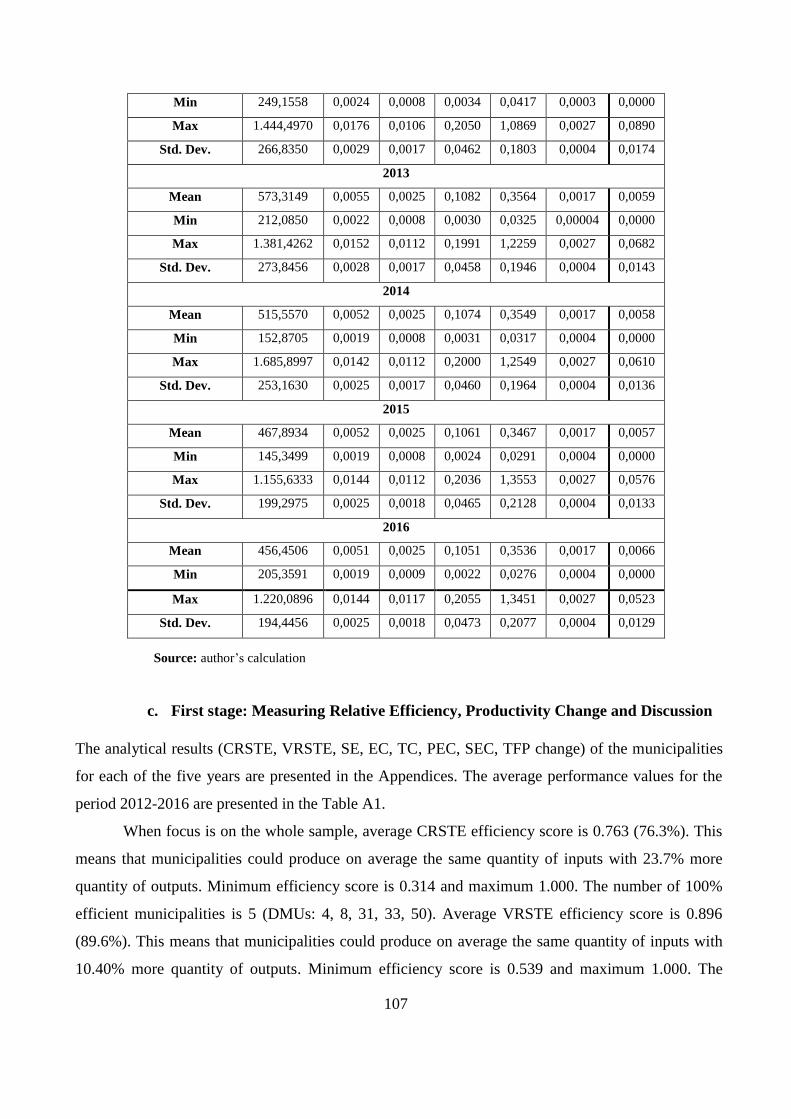
Table 1 reports descriptive statistics of inputs and outputs (means, standard deviations maxima and
minima). The findings show that the average trend for X1, X2, Y1, Y2 and Y4 is downward, since
most output variables tend to decrease over the period with the exception of the X3 and Y3 that remain
more stable. The average total annual expenditures per inhabitant is about 456-573€. The average
number of employees per inhabitant is 0.0051-0.0059. The average number of vehicles-machinery
per inhabitant is 0.0025. The average number per inhabitant of pupils enrolled in the pre-primary /
primary / secondary municipal infrastructures is 0.1051-0.1093. The average total quantity per
inhabitant is 0.3467-0.3626 and the average number of beneficiaries from municipal grants per
inhabitant is 0.0057-0.0070. Moreover, the average total annual expenditures per inhabitant of Central
Greece is 546,12€ whereas the average total annual expenditures per inhabitant of Thessaly is
476,43€. This means that the municipalities of the Region of Central Greece spend more per
inhabitant compared to the municipalities in the region of Thessaly.
Table 1. Descriptive statistics of input and output variables by year
Statistics /
Variable
Inputs Outputs
Thessaly & Central Greece
X1 X2 X3 Y1 Y2 Y3 Y4
2012
Mean 543,1554 0,0059 0,0025 0,1093 0,3626 0,0017 0,0070
107
Min 249,1558 0,0024 0,0008 0,0034 0,0417 0,0003 0,0000
Max 1.444,4970 0,0176 0,0106 0,2050 1,0869 0,0027 0,0890
Std. Dev. 266,8350 0,0029 0,0017 0,0462 0,1803 0,0004 0,0174
2013
Mean 573,3149 0,0055 0,0025 0,1082 0,3564 0,0017 0,0059
Min 212,0850 0,0022 0,0008 0,0030 0,0325 0,00004 0,0000
Max 1.381,4262 0,0152 0,0112 0,1991 1,2259 0,0027 0,0682
Std. Dev. 273,8456 0,0028 0,0017 0,0458 0,1946 0,0004 0,0143
2014
Mean 515,5570 0,0052 0,0025 0,1074 0,3549 0,0017 0,0058
Min 152,8705 0,0019 0,0008 0,0031 0,0317 0,0004 0,0000
Max 1.685,8997 0,0142 0,0112 0,2000 1,2549 0,0027 0,0610
Std. Dev. 253,1630 0,0025 0,0017 0,0460 0,1964 0,0004 0,0136
2015
Mean 467,8934 0,0052 0,0025 0,1061 0,3467 0,0017 0,0057
Min 145,3499 0,0019 0,0008 0,0024 0,0291 0,0004 0,0000
Max 1.155,6333 0,0144 0,0112 0,2036 1,3553 0,0027 0,0576
Std. Dev. 199,2975 0,0025 0,0018 0,0465 0,2128 0,0004 0,0133
2016
Mean 456,4506 0,0051 0,0025 0,1051 0,3536 0,0017 0,0066
Min 205,3591 0,0019 0,0009 0,0022 0,0276 0,0004 0,0000
Max 1.220,0896 0,0144 0,0117 0,2055 1,3451 0,0027 0,0523
Std. Dev. 194,4456 0,0025 0,0018 0,0473 0,2077 0,0004 0,0129
Source: author’s calculation
c. First stage: Measuring Relative Efficiency, Productivity Change and Discussion
The analytical results (CRSTE, VRSTE, SE, EC, TC, PEC, SEC, TFP change) of the municipalities
for each of the five years are presented in the Appendices. The average performance values for the
period 2012-2016 are presented in the Table A1.
When focus is on the whole sample, average CRSTE efficiency score is 0.763 (76.3%). This
means that municipalities could produce on average the same quantity of inputs with 23.7% more
quantity of outputs. Minimum efficiency score is 0.314 and maximum 1.000. The number of 100%
efficient municipalities is 5 (DMUs: 4, 8, 31, 33, 50). Average VRSTE efficiency score is 0.896
(89.6%). This means that municipalities could produce on average the same quantity of inputs with
10.40% more quantity of outputs. Minimum efficiency score is 0.539 and maximum 1.000. The

108
number of 100% efficient municipalities is 17 (DMUs: 4, 8, 13, 14, 26, 29, 30, 31, 33, 34, 35, 36, 40,
44, 45, 47, 50). Furthermore, municipalities operate close to the optimal scale, SE=0.851 (refrain
14.90% from the optimal scale).The results are consistent with previous studies (Worthington and
Dollery 2000; Pevcin, 2014; Lo Storto, 2016).
The findings also show that relatively large municipalities with population criteria
(population>average population) have comparatively higher efficiency rates (CRSTE=0.874,
VRSTE=0.924, SE=0.942) than smaller municipalities (CRSTE=0.727, VRSTE=0.887, SE=0.822).
Relatively large municipalities are producing more quantity of outputs than relatively small ones. Also,
municipalities of Thessaly could on average produce the same quantity of inputs with 20.7% more
quantity of outputs, whereas municipalities of Central Greece with 26.80%. Table 2 reports the number
of municipalities and the average efficiency scores and shows that 18 municipalities have average
CRSTE ranging between 0.600 and 0.800, 31 municipalities have average VRSTE ranging between
0.900 and 1.000 and 27 municipalities have average SE ranging between 0.900 and 1.000.
Table 2. Number of municipalities & efficiency score
EFFICIENCY
SCORE CRSTE VRSTE SE
[0 - 0.600) 9 1 4
[0.600 – 0.800) 18 11 12
[0.800 – 0.900) 8 7 7
[0.900- 1.000] 15 31 27
Source: author’s calculation
The Malmquist TFP results (Agasisti et al., 2015; Sung, 2007; Kutlar and Bakirci, 2012)
indicate that municipalities experienced an approx. 0.6% increase in average productivity. On
examining the components of the productivity change, it becomes evident that the productivity gain
may be primarily attributed to a change in relative efficiency and especially to the combination of both
positive annual average EC (2.7%) and negative annual average TC (-2.1%). On average,
improvements in PEC are the main reasons for the improvements in EC. The average PEC, which
measures changes in VRSTE, indicates that there is an improvement of 1.5% over the examined period.
Municipalities of Central Greece have higher values of TFP change than municipalities of Thessaly.
Also, municipalities of Central Greece have higher values of EC and TC than municipalities of
Thessaly. The results show that 34 Municipalities have TFP change >1, ranging between 0,10% and
14,40%.

109
15 municipalities have TFP change < 1 ranging between –0.10% and –46.40%. This means
that it was poor technology which needed to be updated or that it has not been used best-practice
technology in the management. 12% of Municipalities have no change in efficiency, 60% of
municipalities (experience increase (EC > 1) and the remaining 28% decrease (EC < 1). As a next step,
we classify municipalities on the basis of their average VRSTE in the years 2012-2016 and the results
of the average TFP change in the period 2012–2016.
Figure 1. Average VRSTE and TFP change
Source: author’s calculation
The incision of the axes is the point O (mean VRSTE = 0.870, mean TFP = 0.010). The four
groups in Figure 1 are characterized as follows:
Quadrant A: High efficiency and positive productivity growth.
Municipalities (DMUS: 35, 46, 19, 32, 43, 23, 38, 11, 41, 39, 31, 36, 30, 1, 34, 14, 26) have
the best performance and can be benchmarks for other municipalities. This suggests that they should
maintain their position by continuing to implement good strategies so as to fulfill their mission.
Quadrant Β: Low efficiency and positive productivity growth.
Municipalities (DMUS: 20, 7, 5, 2, 21, 22, 37, 17, 24, 3, 28, 12, 18,) with medium to low
efficiency have positive productivity growth. Special consideration should be given to these

110
municipalities in order to improve their efficiency by implementing current strategies of productivity
improvement.
Quadrant C: High efficiency and negative productivity growth.
Municipalities (DMUS: 42, 29, 16, 13, 40, 4, 45, 47, 33, 9, 10, 50, 49, 8, 44) still maintains a
good efficiency in managing their resources, in spite of their productivity decline. Moreover, if they
do not want to lose their current position they have to maintain a rapid growth, by maintaining positive
technological change.
Quadrant D: Low efficiency and negative productivity growth.
Municipalities in the bottom-left quadrant (DMUS: 15, 25, 6, 27, 48) are those that have
medium-low efficiency in managing their resources. Special attention should be given to those
municipalities so as to diagnose their problems and to improve their efficiency.
d. Second Stage: OLS Analysis/Tobit Analysis
At the second stage of our two step analysis, differences in the DEA efficiency scores are explained
by characteristics of municipalities. The regression model explaining variation of efficiency scores
among municipalities were estimated with the 2012-2016 data. OLS and Tobit are the estimation
models.
Table 3. OLS Regression analysis results
Variables Coefficient
Z1
1.384
(1.22)
n.s.
Z2
-0.003
(-0.09)
n.s.
Ζ3
0.129
(2.14)
**
Z4
0.0004
(1.62)
n.s.
Z5
0.033
(0.48)
ns
Z6 -0.006

111
Variables Coefficient
(-0.75)
ns
Z7
-0.00003
(-0.11)
ns
R
0.2326
Adj. R2 0.1047
F 1.82
Note: 1)***, **, * level of statistic significance 1%, 5% και 10%, n.s. non-significant
2) Numbers in parentheses show the t- statistic values
Source: author’s calculation
Table 3 reports the results of the OLS regression analysis and presents the variables that were
considered in the DEA second stage analysis: number of unemployed as percentage of population (Z1),
education level of mayor (Z2), type of municipality (Z3), population density (Z4), mayor’s gender
(Z5), number of amalgated municipalities (Z6), distance from the center of the region (Z7). The use
of these variables are consistent with the existing literature. For this purpose, the exogenous variables
regressed with efficiency score include values between zero and one. Relationships between these
variables in the regression model are formulated as follows:
(5)
where, i is the municipality to i (i = 1, ..., 50), T.E. is the efficiency score, and є is the error
term. A positive sign of the coefficient indicates that this latter is positively associated to VRSTE while
a negative sign denotes an unfavorable association. The value of R2 is satisfactory, since the data are
cross-section and show a satisfactory interpretive capacity of the equation. Prob(F-statistics) depicts
the probability of null hypothesis being true. As per the above results, probability is close to zero
(1.82). This implies that, overall, the regression is meaningful. It turned out that number of unemployed
as percentage of population, education level of mayor, mayor’s gender, number of amalgamated
municipalities, distance from the center of the region and population density did not explain efficiency
differences and had no effect on efficiency. Of the variables examined, only Z3 have statistically
significant and positive effect on VRSTE. As expected, the type pf municipality is related to high

112
efficiency. Our location variable (Z3) proved to be the most significant explanatory variable in our
estimation results, getting high t-value.
The results are further interpreted using the Tobit model. The results are given in Table 4 and
show that Z3, Z4 have statistically significant and positive effect on VRSTE (Ζ3 higher statistical
effect than Z4). This relationship, according to Borger and Kerstens (1996) and Afonso and Fernandes
(2008), is interpreted in a sense that a dense residential structure with a portion of the population who
live in it, has relatively higher positive effect on efficiency that have a population structure that is
relatively less dense. For the data analysis we use the STATA® Statistics / Data Analysis 14.2 SE
software package (1985-2015 Stata Corp LLC, USA).
Table 4. Tobit Regression analysis results
Variables Coefficient
Z1
1.343
(1.27)
n.s.
Z2
-0.001
(-0.03)
n.s.
Ζ3
0.129
(2.28)
**
Z4
0.0004
(1.76)
*
Z5
0.033
(0.51)
ns
Z6
-0.006
(-0.80)
ns
Z7
-0.00002
(-0.08)
ns
LR chi2(7) 12.86
Pseudo R2 -0.2035
Log likelihood 38.018
/sigma 0.107

113
Variables Coefficient
Note: 1)***, **, * level of statistic significance 1%, 5% και 10%, n.s. non-significant
2) Numbers in parentheses show the t- statistic values
Source: author’s calculation
5. Concluding remarks and policy implications
This paper contributes to the literature on the empirical understanding of relative efficiency and
productivity change in the two Greek representative regions (Thessaly and Central Greece).
Additionally, it determinates the factors which affect the efficiency coefficients. From empirical
analysis and discussion, the following key conclusions are drawn:
i. The average values of technical efficiency under variable and constant returns to scale,
scale efficiency and total factor productivity change of the municipalities are in line with
the results of European and non- European countries.
ii. Over the five years considered, there was a gradual improvement (year by year) of the
average efficiency and productivity of the municipalities.
iii. The best performance (efficiency> mean VRSTE, productivity> mean TFP) have 17 of
the 50 municipalities (34%) and they can be benchmarks for the other municipalities.
The rest of them should try to learn from best practices in order to improve their own
performance. That is paramount for a better use of scarce public resources in the context
of the European Union's strategic direction to optimize the resource use.
iv. Relatively large municipalities with population criteria have comparatively better
performances on average than relatively small ones.
v. The environmental variables - population density and type of municipality - have
statistically significant positive effect on the municipality efficiency score.
vi. Municipalities of Thessaly have on average better performance than municipalities of
Central Greece.
In fact, by giving insight into the causes of inefficiency, this helps to further identify the
reasons for local inefficient behavior and may support effective policy measures to correct and or
control them. Our study also helps to the ongoing discussion about the need and form of reforms in
basic service provision. The proposals have included increasing municipality sizes by mergers or
increasing voluntary cooperation of municipalities to make them more efficient. Decision makers at
both municipal and central government levels have to acknowledge the significance of the findings.

114
Appropriate policy measures will lead to an improvement in the performance of all municipalities
and, especially, of those with low performance. By merging two or more municipalities into a single
new municipality or sharing the provision of public services creating an association or a consortium
of municipalities has also benefits in terms of elimination of administrative and political body
duplication. Also, the establishment of an observatory that aims to systematically measure and
monitor the efficiency and productivity change of municipalities contributes positively to linking
performance to resource allocation. In this direction, the introduction of an incentive-based system
which will reward efficient municipalities and trigger surveillance programmes for those who need
to improve is very important as well.
Undoubtedly, a need exists to continue the study and to improve certain factors that have not
been adequately considered herein. Further research is needed to broaden the scope of services
analyzed, with different combinations of inputs and outputs. Besides, repeating the survey year after
year would enhance comparisons and allow investigating the evolution of municipal efficiency while
the country has come out of the strict monitoring of the memorandums.
References
Afonso, A. and Fernandes, S. (2003). Efficiency of local government spending: evidence for
the Lisbon region. [online] SSRN. Available at: <https://ssrn.com/abstract=470481> [Accessed 1
February 2021].
Afonso, A. and Fernandes, S. (2006). Measuring local government spending efficiency:
evidence for the Lisbon region. [online] ResearchGate, pp.39–53. Available at:
<https://www.researchgate.net/publication/24087975_Measuring_Local_Government_Spending_Ef
ficiency_Evidence_for_the_Lisbon_Region> [Accessed 15 January 2021].
Afonso, A. and Fernandes, S. (2008). Assessing and explaining the relative efficiency of local
government. The Journal of Socio-Economics, [online] 37(5), pp.1946–1979. Available at:
<https://www.sciencedirect.com/science/article/abs/pii/S105353570700073X> [Accessed 1
February 2021].
Agasisti, T., Dal Bianco, A. and Griffini, M. (2016). The public sector fiscal efficiency in
Italy: the case of Lombardy municipalities in the provision of the essential public services.
ECONOMIA PUBBLICA, [online] pp.59–84. Available at:
<https://www.researchgate.net/publication/305712202_The_public_sector_efficiency_in_Italy_The
_case_of_Lombardy_municipalities_in_the_provision_of_the_essential_public_services>
[Accessed 9 February 2021].

115
Andrews, R. and Entwistle, T. (2015). Public–private partnerships, management capacity and
public service efficiency. Policy & Politics, [online] 43(2), pp.273–290. Available at:
<https://www.researchgate.net/publication/275719873_Public-
private_partnerships_management_capacity_and_public_service_efficiency> [Accessed 15 January
2021].
Aparicio, J., Cordero, J.M. and Pastor, J.T. (2016). Productivity change of Portuguese
municipalities after local reforms. Applied Economics Letters, [online] 24(12), pp.878–881.
Available at:
<https://www.tandfonline.com/doi/abs/10.1080/13504851.2016.1237738?journalCode=rael20>
[Accessed 9 February 2021].
Arcelus, F.J., Arocena, P., Cabases, F. and Pascual, P. (2011). On the Cost-Efficiency of
Service Delivery in Small Municipalities. Regional Studies, 49(9), pp.1469–1480.
Asatryan, Z. and De Witte, K. (2015). Direct Democracy and Local Government Efficiency.
European Journal of Political Economy, 39, pp.58–66.
Ashworth, J., Geys, B., Heyndels, B. and Wille, F. (2014). Competition in the political arena
and local government performance. Applied Economics, [online] 46(19), pp.2264–2276. Available
at: <https://www.tandfonline.com/doi/abs/10.1080/00036846.2014.899679> [Accessed 1 February
2021].
Balaguer-Coll, M.T., Prior, D. and Tortosa-Ausina, E. (2009). Decentralization and efficiency
of local government. The Annals of Regional Science, [online] 45(3), pp.571–601. Available at:
<https://link.springer.com/article/10.1007/s00168-009-0286-7> [Accessed 15 January 2021].
Balaguer-Coll, M.T., Prior, D. and Tortosa-Ausina, E. (2010). Devolution Dynamics of
Spanish Local Government. Environment and Planning A: Economy and Space, [online] 42(6),
pp.1476–1495. Available at: <https://journals.sagepub.com/doi/abs/10.1068/a42506> [Accessed 9
February 2021].
Balaguer-Coll, M.T., Prior, D. and Tortosa-Ausina, E. (2012). Output complexity,
environmental conditions, and the efficiency of municipalities. Journal of Productivity Analysis,
[online] 39(3), pp.303–324. Available at: <https://link.springer.com/article/10.1007/s11123-012-
0307-x> [Accessed 9 February 2021].
Banker, R.D., Charnes, A. and Cooper, W.W. (1984). Some Models for Estimating Technical
and Scale Inefficiencies in Data Envelopment Analysis. Management Science, 30(9), pp.1078–1092.
Barone, G. and Mocetti, S. (2011). Tax morale and public spending inefficiency. International
Tax and Public Finance, 18(6), pp.724–749.

116
Benito, B., Bastida, F. and Garcia, J. (2010). Explaining differences in efficiency: an
application to Spanish municipalities. Applied Economics, [online] 42(4), pp.515–528. Available at:
<https://ideas.repec.org/a/taf/applec/v42y2010i4p515-528.html> [Accessed 15 February 2021].
Borge, L.-E., Falch, T. and Tovmo, P. (2008). Public sector efficiency: the roles of political
and budgetary institutions, fiscal capacity, and democratic participation. Public Choice, [online]
136(3-4), pp.475–495. Available at: <https://link.springer.com/article/10.1007/s11127-008-9309-7>
[Accessed 15 January 2021].
Bruns, C. and Himmler, O. (2011). Newspaper Circulation and Local Government Efficiency.
The Scandinavian Journal of Economics, [online] 113(2), pp.470–492. Available at:
<https://www.jstor.org/stable/23016844?seq=1> [Accessed 15 January 2021].
Caves, D.W., Christensen, L.R. and Diewert, W.E. (1982). The Economic Theory of Index
Numbers and the Measurement of Input, Output, and Productivity. Journal of the Econometric
Society, [online] 50(6), pp.1393–1414. Available at:
<https://www.jstor.org/stable/1913388?origin=crossref> [Accessed 1 February 2021].
Charnes, A., Cooper, W.W. and Rhodes, E. (1978). Measuring the efficiency of decision
making units. European Journal of Operational Research, 2(6), pp.429–444.
Coelli, T. (1996). A Guide to DEAP Version 2.1: A Data Envelopment Analysis (Computer)
Program. [online] Armidale, Australia: University of New England. Available at:
<https://www.owlnet.rice.edu/~econ380/DEAP.PDF> [Accessed 1 February 2021].
Cordero, J.M., Pedraja-Chaparro, F., Pisaflores, E.C. and Polo, C. (2017). Efficiency
assessment of Portuguese municipalities using a conditional nonparametric approach. Journal of
Productivity Analysis, [online] 48(1), pp.1–24. Available at:
<https://link.springer.com/article/10.1007/s11123-017-0500-z> [Accessed 9 February 2021].
Debreu, G. (1951). The Coefficient of Resource Utilization. Journal of the Econometric
Society, [online] 19(3), pp.273–292. Available at: <https://www.jstor.org/stable/1906814?seq=>
[Accessed 9 February 2021].
Dollery, B. and Van der Westhuizen, G. (2009). Efficiency measurement of basic service
delivery at South African district and local municipalities. The Journal for Transdisciplinary
Research in Southern Africa, 5(2), p.13.
Färe, R., Grosskopf, S., Logan, J. and Lovell, C.A.K. (1985). Measuring Efficiency in
Production: With an Application to Electric Utilities. Managerial Issues in Productivity Analysis,
[online] 7, pp.185–214. Available at: <https://link.springer.com/chapter/10.1007/978-94-009-4982-
9_8> [Accessed 12 February 2021].

117
Färe, R., Grosskopf, S., Norris, M. and Zhang, Z. (1994). Productivity Growth, Technical
Progress, and Efficiency Change in Industrialized Countries. The American Economic Review, 84(1),
pp.66–83.
Farrell, M.J. (1957). The Measurement of Productive Efficiency. Journal of the Royal
Statistical Society. Series A (General), 120(3), pp.253–290.
Geys, B. (2006). Looking across borders: A test of spatial policy interdependence using local
government efficiency ratings. Journal of Urban Economics, [online] 60(3), pp.443–462. Available
at: <https://www.sciencedirect.com/science/article/abs/pii/S0094119006000404> [Accessed 12
February 2021].
Geys, B., Heinemann, F. and Kalb, A. (2010). Voter involvement, fiscal autonomy and public
sector efficiency: Evidence from German municipalities. European Journal of Political Economy,
26(2), pp.265–278.
Geys, B., Heinemann, F. and Kalb, A. (2012). Local Government Efficiency in German
Municipalities. Raumforschung und Raumordnung, 71(4), pp.283–293.
Giménez, V.M. and Prior, D. (2007). Long- and Short-Term Cost Efficiency Frontier
Evaluation: Evidence from Spanish Local Governments. Fiscal Studies, 28(1), pp.121–139.
Grossman, P.J. (1999). Public Sector Technical Inefficiency in Large U.S. Cities. Journal of
Urban Economics, [online] 46(2), pp.278–299. Available at:
<https://www.sciencedirect.com/science/article/abs/pii/S0094119098921222> [Accessed 9 February
2021].
Helland, L. and Sørensen, R.J. (2015). Partisan bias, electoral volatility, and government
efficiency. Electoral Studies, 39, pp.117–128.
Ibrahim1, F.W. and Salleh2, M.F.M. (2006). MyJurnal - Malaysian Citation Centre.
Malaysian Journal of Economic Studies, 43(1/2), pp.85–95.
Kalb, A. (2010). The Impact of Intergovernmental Grants on Cost Efficiency: Theory and
Evidence from German Municipalities. Economic Analysis and Policy, 40(1), pp.23–48.
Kalb, A., Geys, B. and Heinemann, F. (2012). Value for money? German local government
efficiency in a comparative perspective. Applied Economics, 44(2), pp.201–218.
Koopmans, T. (1951). Efficient Allocation of Resources. Journal of the Econometric Society,
19(4), pp.455–465.
Kutlar, A., Bakirci, F. and Yüksel, F. (2012). An analysis on the economic effectiveness of
municipalities in Turkey. African Journal of Marketing Management, 4(3), pp.80–98.

118
Lampe, H.W., Hilgers, D. and Ihl, C. (2015). Does accrual accounting improve municipalities’
efficiency? Evidence from Germany. Applied Economics, 47(41), pp.4349–4363.
Lin, M.-I., Lee, Y.-D. and Ho, T.-N. (2011). Applying integrated DEA/AHP to evaluate the
economic performance of local governments in China. European Journal of Operational Research,
209(2), pp.129–140.
lo Storto, C. (2016). The trade-off between cost efficiency and public service quality: A non-
parametric frontier analysis of Italian major municipalities. Cities, 51, pp.52–63.
Loikkanen, H, Susiluoto, I & Funk, M (2011). The role of city managers and external
variables in explaining efficiency differences of Finnish municipalities. HECER Discussion Paper,
no. 312, HECER, Helsinki.
Loikkanen, H. and Susiluoto, I. (2005). COST EFFICIENCY OF FINNISH
MUNICIPALITIES IN BASIC SERVICE PROVISION 1994-2002. Urban Public Economics Review,
4, pp.39-64.
Mahabir, J. (2014). Quantifying Inefficient Expenditure in Local Government: A Free
Disposable Hull Analysis of a Sample of South African Municipalities. South African Journal of
Economics, 82(4), pp.493–513.
Nakazawa, K. (2013). Cost Inefficiency of Municipalities after Amalgamation. Procedia
Economics and Finance, 5, pp.581–588.
Nakazawa, K. (2014). Does the Method of Amalgamation Affect Cost Inefficiency of the New
Municipalities? Open Journal of Applied Sciences, 4(4), pp.143–154.
Narbón-Perpiñá, I. and De Witte, K. (2017). Local governments’ efficiency: a systematic
literature review-part II. International Transactions in Operational Research, 25(4), pp.1107–1136.
Narbón‐Perpiñá, I. and De Witte, K. (2017). Local governments’ efficiency: a systematic
literature review—part I. International Transactions in Operational Research, 25(2), pp.431–468.
Nijkamp, P. and Suzuki, S. (2009). A Generalized Goals-achievement Model in Data
Envelopment Analysis: an Application to Efficiency Improvement in Local Government Finance in
Japan. Spatial Economic Analysis, 4(3), pp.249–274.
Nikolov, M. and Hrovatin, N. (2013). Cost efficiency of Macedonian municipalities in service
delivery: does ethnic fragmentation matter? Lex Localis, 11(3), pp.743–775.
Nolan, J.F., Moore, A.T. and Segal, G. (2003). Putting Out the Trash: Measuring Municipal
Service Efficiency in U.S. Cities. Urban Affairs Review,

119
Peng, S.-C.P.S.-Y.L.C.-J. and Wu, P.-C. (2011). Local government efficiency evaluation:
Consideration of undesirable outputs and super-efficiency. African Journal of Business Management,
5(12), pp.4746–4754.
Pérez-López, G., Prior, D. and Zafra-Gómez, J.L. (2015). Rethinking New Public
Management Delivery Forms and Efficiency: Long-Term Effects in Spanish Local Government:
Table 1. Journal of Public Administration Research and Theory, 25(4), pp.1157–1183.
Pevcin, P. (2014). Costs and Efficiency of Municipalities in Slovenia | Lex localis - Journal
of Local Self-Government. Lex Localis, 11(3), pp.417–429.
Pougkakioti, I.D. and Tsamadias, C. (2020). Measuring the efficiency and Productivity
Change of Municipalities: empirical evidence from Greek Municipalities over the time period 2013-
2016. Regional Science Inquiry, XII(1), pp.55–74.
Prieto, A.M. and Zofio, J.L. (2001). Evaluating Effectiveness in Public Provision of
Infrastructure and Equipment: The Case of Spanish Municipalities. Journal of Productivity Analysis,
15(1), pp.41–58.
Radulovic, B. and Dragutinovic, S. (2015). Efficiency of Local Self-Governments in Serbia:
An SFA Approach. Industrija, 43(3), pp.123–142.
Revelli, F. (2010). Spend More, Get More? An Inquiry into English Local Government
Performance. Oxford Economic Papers, 62(1), pp.185–207.
Revelli, F. and Tovmo, P. (2007). Revealed yardstick competition: Local government
efficiency patterns in Norway. Journal of Urban Economics, 62(1), pp.121–134.
Sanchez, R. and Pacheco, F. (2014). A Longitudinal Parametric Approach to Estimate Local
Government Efficiency. Germany: Munich University Library.
Shiyi, C. and Jun, Z. (2009). Empirical research on fiscal expenditure efficiency of local
governments in China: 1978–2005. Social Sciences in China, [online] 30(2), pp.21–34. Available at:
https://www.tandfonline.com/doi/abs/10.1080/02529200902981103 [Accessed 15 January 2021].
Sørensen, R.J. (2014). Political competition, party polarization, and government performance.
Public Choice, 161(3/4), pp.427–450.
Sousa, M. da C.S. de, Cribari-Neto, F. and Stosic, B.D. (2005). Explaining DEA Technical
Efficiency Scores in an Outlier Corrected Environment: The Case of Public Services in Brazilian
Municipalities. Brazilian Review of Econometrics, [online] 25(2), pp.287–313. Available at:
<http://bibliotecadigital.fgv.br/ojs/index.php/bre/article/view/2507> [Accessed 9 February 2021].
Šťastná, L. and Gregor, M. (2014). Public sector efficiency in transition and beyond: evidence
from Czech local governments. Applied Economics, 47(7), pp.680–699.

120
Sung, N. (2007). Information technology, efficiency and productivity: evidence from Korean
local governments. Applied Economics, 39(13), pp.1691–1703.
Worthington, A.C. and Dollery, B.E. (2000). Measuring Efficiency in Local Governments’
Planning and Regulatory Function. Public Productivity & Management Review, 23(4), pp.469–485.
Yusfany, A. (2015). The Efficiency Of Local Governments And Its Influence Factors.
International Journal of Technology Enhancements and Emerging Engineering Research, 4(10),
pp.219–241.

121
Appendices
Table A1. Average Efficiency with CRS/VRS, (O.O.)
DMUs
Output - oriented
TE SE Productivity Change
CRS Rank VRS Rank S.E Rank EC TC PEC SEC
Total Factor
Productivity
Change
1 0.991 6 0.994 19 0.997 6 1.011 1.016 1.008 1.003 1.027
2 0.512 45 0.644 49 0.798 35 1.007 1.024 1.026 0.981 1.031
3 0.651 38 0.697 46 0.938 22 1.098 0.925 1.101 0.997 1.016
4 1.000 1 1.000 1 1.000 1 1.000 0.992 1.000 1.000 0.992
5 0.502 46 0.539 50 0.930 25 0.973 1.043 1.000 0.973 1.015
6 0.628 40 0.799 39 0.784 38 1.054 0.946 1.031 1.022 0.997
7 0.595 42 0.696 47 0.850 32 1.133 0.943 1.044 1.085 1.068
8 1.000 1 1.000 1 1.000 1 1.000 0.928 1.000 1.000 0.928
9 0.864 17 0.934 27 0.927 26 0.967 1.016 1.001 0.966 0.983
10 0.703 32 0.962 22 0.731 42 0.968 1.018 1.001 0.967 0.986
11 0.838 21 0.945 24 0.885 28 1.051 0.970 1.026 1.025 1.020
12 0.678 34 0.784 41 0.866 29 1.009 0.999 1.021 0.988 1.009
13 0.646 39 1.000 1 0.646 45 1.079 0.926 1.000 1.079 0.999
14 0.957 10 1.000 1 0.957 15 1.004 1.013 1.000 1.004 1.017
15 0.673 36 0.846 35 0.798 35 0.985 1.017 1.026 0.960 1.001
16 0.939 13 0.960 23 0.973 9 1.095 0.913 1.057 1.036 1.000
17 0.773 26 0.830 36 0.932 24 1.078 0.967 1.076 1.002 1.043
18 0.607 41 0.810 37 0.749 40 1.047 0.964 1.001 1.047 1.010
19 0.924 14 0.936 26 0.986 7 1.036 1.029 1.036 1.001 1.067
20 0.736 30 0.870 33 0.838 33 1.153 0.992 1.072 1.076 1.144
21 0.394 48 0.706 44 0.560 48 1.110 0.951 0.983 1.129 1.056
22 0.426 47 0.691 48 0.617 46 1.055 0.990 0.997 1.059 1.045
23 0.853 19 0.928 28 0.920 27 0.992 1.041 1.021 0.971 1.033
24 0.577 43 0.794 40 0.726 43 1.032 0.998 1.009 1.023 1.029
25 0.830 22 0.860 34 0.965 11 1.074 0.934 1.067 1.006 1.003
26 0.964 7 1.000 1 0.964 12 1.020 0.997 1.000 1.020 1.017
27 0.760 27 0.804 38 0.945 19 1.026 0.958 1.033 0.993 0.982
28 0.676 35 0.716 43 0.944 20 0.984 1.035 0.994 0.990 1.018
29 0.851 20 1.000 1 0.851 31 0.988 1.020 1.000 0.988 1.008
30 0.960 8 1.000 1 0.960 13 1.008 1.028 1.000 1.008 1.036
31 1.000 1 1.000 1 1.000 1 1.020 0.997 1.000 1.020 1.017
32 0.906 15 0.922 30 0.983 8 1.026 0.958 1.033 0.993 0.982
33 1.000 1 1.000 1 1.000 1 1.000 0.976 1.000 1.000 0.976
34 0.564 44 1.000 1 0.564 47 1.017 1.004 1.000 1.017 1.021
35 0.314 50 1.000 1 0.314 50 1.115 0.999 1.000 1.115 1.113
36 0.794 25 1.000 1 0.794 37 1.028 1.021 1.000 1.028 1.049
37 0.737 29 0.780 42 0.944 20 1.046 1.011 1.023 1.022 1.057
38 0.878 16 0.909 31 0.967 10 1.000 1.024 0.999 1.001 1.024
39 0.946 12 0.998 18 0.948 18 1.014 1.006 1.002 1.012 1.021
40 0.951 11 1.000 1 0.951 17 0.968 1.025 1.000 0.968 0.993
41 0.679 33 0.979 21 0.692 44 1.052 0.975 1.010 1.042 1.026
42 0.710 31 0.943 25 0.754 39 0.992 1.016 1.035 0.958 1.007
43 0.795 24 0.924 29 0.859 30 1.042 0.992 1.024 1.018 1.034
44 0.821 23 1.000 1 0.821 34 0.980 0.548 1.000 0.980 0.536
45 0.321 49 1.000 1 0.321 49 0.993 0.995 1.000 0.993 0.988
46 0.740 28 0.981 20 0.749 40 1.199 0.914 1.019 1.176 1.096
47 0.960 8 1.000 1 0.960 13 0.988 0.994 1.000 0.988 0.982
48 0.658 37 0.703 45 0.936 23 0.980 0.973 0.988 0.992 0.954
49 0.854 18 0.899 32 0.952 16 0.961 1.000 1.000 0.961 0.961
50 1.000 1 1.000 1 1.000 1 1.000 0.981 1.000 1.000 0.981
Mean 0.763 0.896 0.851 1.027 0.979 1.015 1.012 1.006

122
DMUs
Output - oriented
TE SE Productivity Change
CRS Rank VRS Rank S.E Rank EC TC PEC SEC
Total Factor
Productivity
Change
Mean
Central
Greece
0.732 0.849 0.855
1.039
0.981
1.024
1.015
1.020
Mean
Thessaly 0.793 0.942 0.847
1.015
0.977
1.005
1.010
0.992
Source: Author Calculation
Table A2. Efficiency with CRS/VRS, (O.O.)
Municipality 2012 2013 2014 2015 2016
CRS VRS SE CRS VRS SE CRS VRS SE CRS VRS SE CRS VRS SE
Lamia 0.957 0.970 0.987 1.000 1.000 1.000 1.000 1.000 1.000 1.000 1.000 1.000 1.000 1.000 1.000
Amfiklia-Elatia 0.487 0.605 0.804 0.556 0.614 0.907 0.509 0.656 0.776 0.510 0.676 0.755 0.500 0.670 0.746
Domokos 0.499 0.506 0.986 0.593 0.687 0.863 0.707 0.805 0.879 0.734 0.740 0.992 0.724 0.745 0.972
Lokron 1.000 1.000 1.000 1.000 1.000 1.000 1.000 1.000 1.000 1.000 1.000 1.000 1.000 1.000 1.000
Makrakomi 0.530 0.535 0.989 0.539 0.547 0.985 0.472 0.537 0.879 0.492 0.542 0.908 0.475 0.536 0.887
Molos-Ag.Konstantinou 0.516 0.725 0.711 0.622 0.782 0.795 0.698 0.841 0.830 0.668 0.826 0.808
0.635
0.819
0.776
Stylida 0.434 0.624 0.694 0.568 0.690 0.823 0.603 0.719 0.839 0.658 0.706 0.932 0.714 0.743 0.961
Livadia 1.000 1.000 1.000 1.000 1.000 1.000 1.000 1.000 1.000 1.000 1.000 1.000 1.000 1.000 1.000
Aliartos-Thespieon 0.935 0.936 1.000 0.884 0.888 0.996 0.822 0.905 0.908 0.860 1.000 0.860
0.817
0.939
0.870
Distomo-Arachova-
Antikyra 0.738 0.952 0.775 0.729 0.953 0.765 0.715 0.965 0.740 0.685 0.984 0.696
0.648
0.957
0.677
Thebes 0.771 0.893 0.864 0.678 0.873 0.777 0.950 0.969 0.980 0.848 1.000 0.848 0.942 0.988 0.954
Orchomenos 0.670 0.743 0.903 0.660 0.784 0.842 0.662 0.774 0.855 0.705 0.811 0.870 0.695 0.808 0.860
Tanagra 0.536 1.000 0.536 0.598 1.000 0.598 0.681 1.000 0.681 0.688 1.000 0.688 0.726 1.000 0.726
Chalkida 0.983 1.000 0.983 0.960 1.000 0.960 0.966 1.000 0.966 0.875 1.000 0.875 1.000 1.000 1.000
Dirfyon-Messapion 0.743 0.789 0.941 0.717 0.851 0.843 0.585 0.842 0.695 0.621 0.873 0.711
0.698
0.875
0.798
Eretria 0.695 0.802 0.867 1.000 1.000 1.000 1.000 1.000 1.000 1.000 1.000 1.000 1.000 1.000 1.000
Istiaia-Aidipsos 0.633 0.679 0.932 0.770 0.834 0.923 0.775 0.856 0.906 0.834 0.871 0.958 0.855 0.910 0.940
Karystos 0.552 0.810 0.682 0.629 0.800 0.786 0.606 0.800 0.758 0.581 0.829 0.701 0.665 0.812 0.818
Kymi-Aliveri 0.867 0.869 0.997 0.831 0.876 0.948 0.922 0.937 0.984 1.000 1.000 1.000 1.000 1.000 1.000
Mandoudi-Lake-
Ag.Anna 0.565 0.756 0.747 0.723 0.847 0.854 0.591 0.857 0.690 0.800 0.890 0.899
1.000
1.000
1.000
Skyros 0.323 0.742 0.435 0.372 0.689 0.540 0.399 0.705 0.566 0.386 0.699 0.552 0.490 0.693 0.707
Karpenisi 0.368 0.674 0.546 0.422 0.694 0.608 0.450 0.712 0.632 0.436 0.708 0.615 0.456 0.665 0.686
Agrafa 0.844 0.858 0.984 0.913 0.945 0.966 0.846 0.958 0.883 0.846 0.946 0.894 0.816 0.933 0.875
Delphi 0.574 0.783 0.733 0.495 0.772 0.642 0.589 0.798 0.738 0.574 0.805 0.713 0.651 0.811 0.803
Dorida 0.676 0.726 0.931 0.839 0.846 0.992 0.830 0.859 0.966 0.907 0.925 0.981 0.899 0.943 0.953
Larisa 0.923 1.000 0.923 0.932 1.000 0.932 0.986 1.000 0.986 0.977 1.000 0.977 1.000 1.000 1.000
Agia 0.669 0.710 0.942 0.799 0.831 0.961 0.804 0.852 0.944 0.786 0.817 0.961 0.741 0.810 0.915
Elassona 0.696 0.712 0.978 0.727 0.740 0.983 0.687 0.735 0.935 0.617 0.697 0.886 0.651 0.694 0.938
Kileler 0.884 1.000 0.884 0.824 1.000 0.824 0.828 1.000 0.828 0.875 1.000 0.875 0.843 1.000 0.843
Tempi 0.970 1.000 0.970 0.901 1.000 0.901 0.928 1.000 0.928 1.000 1.000 1.000 1.000 1.000 1.000
Tirnavos 1.000 1.000 1.000 1.000 1.000 1.000 1.000 1.000 1.000 1.000 1.000 1.000 1.000 1.000 1.000
Farsala 0.858 0.860 0.998 1.000 1.000 1.000 0.907 0.936 0.969 0.869 0.914 0.951 0.896 0.90 0.995
Karditsa 1.000 1.000 1.000 1.000 1.000 1.000 1.000 1.000 1.000 1.000 1.000 1.000 1.000 1.000 1.000
Argithea 0.510 1.000 0.510 0.545 1.000 0.545 0.612 1.000 0.612 0.608 1.000 0.608 0.546 1.000 0.546
Límni Plastíra 0.218 1.000 0.218 0.306 1.000 0.306 0.349 1.000 0.349 0.360 1.000 0.360 0.336 1.000 0.336
Mouzaki 0.704 1.000 0.704 0.869 1.000 0.869 0.793 1.000 0.793 0.819 1.000 0.819 0.785 1.000 0.785
Palama 0.657 0.726 0.904 0.797 0.805 0.989 0.745 0.793 0.940 0.701 0.779 0.900 0.785 0.795 0.986
Sofades 0.871 0.877 0.994 0.898 0.996 0.901 0.849 0.870 0.976 0.898 0.930 0.966 0.873 0.874 0.999
Volos 0.944 0.992 0.952 0.942 1.000 0.942 0.922 1.000 0.922 0.922 1.000 0.922 1.000 1.000 1.000
Almyros 0.998 1.000 0.998 0.990 1.000 0.990 1.000 1.000 1.000 0.889 1.000 0.889 0.878 1.000 0.878
Zagora-Mouresi 0.627 0.962 0.652 0.669 0.957 0.669 0.664 0.979 0.678 0.665 1.000 0.665 0.768 0.999 0.768
South Pelion 0.660 0.837 0.788 0.769 0.927 0.829 0.790 1.000 0.790 0.691 0.988 0.699 0.638 0.962 0.664
Riga Feraiou 0.801 0.909 0.880 0.771 0.864 0.893 0.752 0.908 0.828 0.703 0.938 0.749 0.946 1.000 0.946
Skiathos 1.000 1.000 1.000 0.573 1.000 0.573 0.783 1.000 0.783 0.829 1.000 0.829 0.921 1.000 0.921

123
Municipality 2012 2013 2014 2015 2016
CRS VRS SE CRS VRS SE CRS VRS SE CRS VRS SE CRS VRS SE
Alonissos 0.325 1.000 0.325 0.337 1.000 0.337 0.308 1.000 0.308 0.319 1.000 0.319 0.317 1.000 0.317
Skopelos 0.438 0.927 0.473 0.522 0.978 0.534 0.853 1.000 0.853 0.980 1.000 0.980 0.905 1.000 0.905
Trikala 1.000 1.000 1.000 0.970 1.000 0.970 0.974 1.000 0.974 0.906 1.000 0.906 0.951 1.000 0.951
Kalambaka 0.678 0.726 0.934 0.626 0.685 0.914 0.663 0.693 0.957 0.700 0.721 0.971 0.625 0.692 0.903
Pylis 0.990 1.000 0.990 0.851 0.853 0.998 0.806 0.842 0.957 0.778 0.802 0.971 0.845 1.000 0.845
Farkadona 1.000 1.000 1.000 1.000 1.000 1.000 1.000 1.000 1.000 1.000 1.000 1.000 1.000 1.000 1.000
Source: Author calculation
Table A3 : Literature Review
Authors Country Years Reference No of municipalities Methodology Inp Outp Envir. Variables
European Countries
Prieto and Zofio (2001)
Spain 1994 209 DEA Χ1
Υ5.1,Υ5.2,Υ6.
2,Υ6.3, Υ7.1,
Υ7.2, Υ7.4
Afonso and Fernandes (2003)
Portugal 2001 51 F.D.H. Χ1 Υ1
Loikkanen and
Susiluoto (2005) Finland 1994-2002 353
T.S.A,
D.E.A.- C.R.S- O.O., O.L.S.
Χ2
Υ7.3, Υ8,
Υ9.2, Υ10.2, Υ10.3,Υ10.4
Z1.1, Z1.3, Z1.5,
Z2.1, Z2.2, Z4.2, Z5.1, Z6.2, Z6.4
Geys (2006) Belgium 2000 304 T.S.A.,S.F.
A.,O.L.S. Χ2
Υ5.2,
Υ7.5, Υ9.2,Υ10.1
Z1.1, Z1.7, Z2.2,
Z3.1, Z3.2, Z4.2, Z4.3, Z4.4, Z6.3
Afonso and
Fernandes (2006) Portugal 2001 51
D.E.A.(I.O.,
O.O.,VRS) Χ1 Υ1
Gimenez and Prior (2007)
Spain 1996 258 T.S.A.,F.D.H.,T.R
Χ3, Χ5, Χ7
Υ2, Υ3, Υ5.2, Υ6.1,
Z1.1, Z1.3, Z2.2, Z2.4, Z2.5, Z2.6
Afonso and Fernandes (2008)
Portugal 2001 278
T.S.A.,D.E.
A.(Ι.Ο.,Ο.Ο.,V.
R.S.), T.R.
Χ1 Υ1 Z1.1, Z1.2, Z1.5, Z2.2, Z5.1
Benito et al.
(2010) Spain 2002 31
T.S.A.,D.E.A.(V.R.S.,O.O.),
Kendall τ test
Χ2, Χ3,
Χ7
Υ6.1, Υ6.3,
Υ7.1, Υ7.2,
Υ7.3, Υ7.4, Υ11
Z1.3, Z2.2, Z2.4, Z3.1, Z4.1, Z4.3, Z4.6,
Z6.4
Geys et al. (2010)
Germany 1998,2002,20
04 987
S.S.A.,S.F.A.
Χ2
Υ2, Υ7.5,
Υ9.1, Υ9.2,
Υ10.2, Υ15
Z1.1, Z3.1, Z3.2, Z3.3, Z4.2
Kalb (2010) Germany 1990-2004 1,111 S.S.A.,S.F.
A. Χ2
Υ2, Υ9.2, Υ10.2, Υ15
Z1.1, Z1.5, Z2.1,
Z2.4, Z3.1, Z3.2, Z4.2,
Z4.6,
Revelli (2010)
England 2002-2007 148 CPA Χ2 Υ1, Υ9.2
Balaguer-Coll et al. (2010a)
Spain 1995, 2000 1,221 F.D.H. Χ2, Χ3, Χ4, Χ7
Υ2 ,Υ5.1,
Υ5.2, Υ6.1, Υ7.4, Υ7.5,
Υ10.4, Υ12
Balaguer-Coll et al. (2010b)
Spain 1995,2000, 2005 1,164 M.I.,F.D.H. Χ1
Υ2, Υ5.1,
Υ5.2, Υ6.1, Υ7.4, Υ7.5,
Υ10.4, Υ12, Υ16
Loikkanen et al (2011)
Finland 1994-1996 353
T.S.A.,D.E.
A. - C.R.S-
O.O., O.L.S.
Χ2
Υ7.3, Υ8,
Υ9.2, Υ10.1,
Υ10.3,Υ10.4
Z1.1, Z1.3, Z1.5,
Z2.1, Z3.1, Z3.2, Z3.3,
Z5.1, Z6.2
Barone and Mocetti (2011)
Italy 2001-2004 1,115 S.F.A. Χ2
Υ4, Υ5.1,
Υ5.2, Υ6.1,
Υ9.1, Υ11
Kalb et al. (2012) Germany 2004 1,015 S.S.A.,
S.F.A. Χ2
Υ2, Υ7.5, Υ9.1,
Υ9.2,Υ10.2,
Υ15
Z1.1, Z2.1, Z2.4,
Z3.1, Z3.2
Balaguer-Coll et
al. (2013) Spain 2000 1,198 Order-m
Χ2, Χ3
Χ4, Χ7
Υ5.1, Υ5.2,
Υ6.1, Υ7.4,
Υ7.5, Υ10.4, Υ12
Z1.1, Z1.2, Z2.2,
Z2.3, Z2.7

124
Authors Country Years Reference No of municipalities Methodology Inp Outp Envir. Variables
Geys et al.
(2013) Germany 2001 1,021
S.S.A.,S.F.
A. Χ2
Υ2, Υ7.5, Υ9.1, Υ9.2,
Υ10.2, Υ15
Z1.1, Z2.1, Z3.2
Ashworth et
al.(2014) Belgium 2000 308
T.S.A.,D.E.
A. - C.R.S. - O.O., B.A.-
Simar and
Wilson,2007
Χ1 Υ5.2, Υ6.1, Υ7.5, Υ9.2,
Υ10.1,Υ10.2
Z1.1, Z1.3, Z2.2, Z3.1, Z3.2, Z4.1, Z4.2,
Z4.3, Z4.4,
Pevcin (2014a) Slovenia 2011 200 S.S.A.,S.F.
A. Χ1
Υ2, Υ9.2,
Υ10.2, Υ15 Z1.1, Z2.1,
ˇStastn´aandGreg
or (2015) Czech republic
1995-1998, 2003-
2008 202
S.S.A.,SFA-
time variant Χ2
Υ3,Υ5.2,
Υ6.1,Υ7.1,Υ7.2,Υ7.4,Υ9.1,Υ
9.2,Υ10.2,Υ10
.4,Υ11,Υ13,
Z1.3, Z1.5, Z3.1, Z3.3, Z4.1, Z4.2, Z4.5,
Z5.1
Arcelus et al. (2015)
Spain 2005 260 S.S.A.,S.F.
A. Χ2
Υ3, Υ4, Υ5.1,
Υ5.2, Υ6.3,
Υ10.2, Υ15
Z1.1, Z4.1, Z4.5, Z5.4, Z6.4, Z6.5
Perez-Lopez et
al. (2015) Spain 2001-2010 1,058
T.S.A.,Order-m, B.A.-
Simar and
Wilson,2007
Χ2
Υ2, Υ3, Υ5.1,
Υ6.1, Υ6.3, Υ7.4, Υ17
Z1.3, Z2.1, Z2.4,
Z3.1, Z3.2, Z4.1, Z4.2, Z4.3, Z4.4,Z4.6, Z6.4
Asatryan and
DeWitte (2015) Germany 2011 2,000
Conditional
FDH Χ1
Υ7.5, Υ9.1,
Υ9.2, Υ10.2
Z1.3, Z2.2, Z3.1,
Z3.3
Lampe et
al.(2015) Germany 2006-2008 396
S.S.A.,
S.F.A. Χ1, Χ2
Υ2, Υ7.5, Υ9.1, Υ9.2,
Υ10.2, Υ15
Z1.1, Z1.6, Z2.1,
Z2.4
Andrews and
Entwistle (2015) England 2007 386
T.S.A.,Rati
os, OLS Χ1 Υ1
Z1.1, Z1.3, Z1.4,
Z1.6, Z1.8, Z2.3, Z3.1, Z4.6, Z5.1, Z6.4 , Z6.5
Cordero et al.
(2016) Portugal 2009-2014 278
Conditional
efficiency Χ1, Χ3
Υ2,Υ4,Υ6.1,
Υ6.3
Z1.1, Z2.1, Z2.2,
Z3.1, Z4.3, Z5.3
Cordero et al. (2017)
Portugal 2009-2014 278 Conditional
efficiency, M.I. Χ1, Χ3
Υ2,Υ4,Υ6.1, Υ6.3
Non-European Countries
Grossman et al.
(1999) U.S.A.
1967,1973,1977,1
982 49
S.S.A.,S.F.
A. - Υ17
Z1.3, Z3.5, Z4.2,
Z5.1, Z6.2
De Sousa et al
(2005) Brazil 2000 4,796
T.S.A.,DEA
"Jackstrap"I.O.,
C.R.S,V.R.S, Quantile
regression
Χ2, Χ3,
Χ8
Υ2, Υ6.1,
Υ6.2, Υ6.3, Υ9.2, Υ10.1
Z1.1, Z2.2, Z2.3,
Z2.4, Z2.7, Z5.1 , Z5.4, Z6.1, Z6.2, Z6.4, Z6.5
Moore et al.(2005)
U.S.A. 1993-1996 46
T.S.A.,D.E.
A.-O.O.- V.R.S
,T.R.
Χ2, Χ3
Υ4, Υ5.2,
Υ6.1, Υ6.3, Υ7.3, Υ7.4,
Υ8, Υ11,
Z4.1, Z5.2, Z5.4, Z6.5
Ibrahim and
Salleh (2006) Malaysia 2000 46 S.F.A. Χ2
Υ2, Υ5.2, Υ6.1, Υ7.4,
Υ12
Sung (2007) Korea 1999-2001 222 T.S.A.,M.I. with
D.E.A.,T.R. Χ1, Χ3,
Υ4, Υ5.2,
Υ6.2, Υ6.3, Υ7.4, Υ10.4
Z1.1, Z1.3, Z2.5,
Z4.1, Z5.2, Z6.1
Revelli and
Tovmo (2007) Norway - 205
T.S.A., RATIO,
O.L.S. Χ6 Υ1
Z1.1, Z3.2, Z3.3,
Z4.1, Z4.3
Borge et al.
(2008) Norway 2001-2005 362-384
T.S.A.,RATIO
,O.L.S. Χ6 Υ1
Z3.1, Z3.2, Z3.3,
Z4.1, Z4.2, Z4.6
Nijkamp and
Suzuki (2009) Japan 2005 34
DEA- DFM-GA (I.O./O.O.-
C.R.S.)
Χ1, Χ3,
Χ4 Υ1, Υ17
Dollery and van
der Westhuizen (2009)
South Africa Fiscal 2006/2007 231 local+46 regional D.E.A(I.O.,Ο.Ο,
V.R.S.,C.R.S) Χ3 Υ6.4
Shiyi and Jun
(2009) China
1978-2005 1993-
2005 27
D.E.A.(V.R.S.,
O.O.) Χ2
Υ9.2, Υ8, Υ3,
Υ6.4, Υ13
Liu et al. (2011) Taiwan 2007 22
D.E.A. super-efficiency
(C.R.S.-V.R.S.-
O.O.)
Χ3 Υ6.2,

125
Authors Country Years Reference No of municipalities Methodology Inp Outp Envir. Variables
Bruns and
Himmler (2011) Norway 2001-2005 362-384
T.S.A.,RATIO,
O.L.S. Χ6 Υ1
Z1.1, Z1.3, Z1.4, Z1.5, Z1.6, Z1.8, Z2.2,
Z3.1, , Z3.2, Z3.5
Lin, Ming-Ian &
Lee, Yuan-Duen & Ho, Tsai-
Neng, (2011)
China 2005-2006 31
DEA
(V.R.S.,C.R.S.,Ο.Ο.) και AHP,
MPI
Χ4 Υ17
Kutlar and
Bakirci (2012) Turkey 2006-2008 27
D.E.A., C.R.S., V.R.S, Ι.Ο.,Ο.Ο,
Μ.Ι.
Χ1, Χ2, Χ3, Χ4,
Χ7
Υ2, Υ9.2,
Υ10.2, Υ8
Nakazawa (2013) Japan 2005 479 S.S.A,S.F.A.,
O.L.S, HCSEs Χ1, Χ3 Υ1
Z1.3, Z1.4, Z1.8,
Z5.2, Z6.3
Nikolov and Hrovatin (2013)
Macedonia - 74
T.S.A.,D.E.A.-
V.R.S-O.O.,
S.F.A.
Χ2
Υ2, Υ5.2,
Υ9.1, Υ9.2,
Υ10.2
Z1.6, Z2.2, Z3.2, Z4.1
Nakazawa (2014) Japan 2005 479 S.F.A., O.L.S,
HCSEs Χ1, Χ2 Υ1
Mahabir (2014) South Africa Fiscal 2005/2006-
2008/2009 129 F.D.H. Χ1
Υ6.1,Υ6.2,Υ6.
3,Υ6.4
Sørensen (2014) Norway 2001-2010 430 T.S.A.,O.L.S
,F.E.R Χ6 Υ1 Z1.3, Z3.1, Z3.2
Pacheco et al.
(2014) Chile 2008-2010 309 S.S.A., S.F.A. Χ2
Υ2, Υ6.1,
Υ6.2, Υ7.4, Υ8, Υ9.2,
Z3.2, Z4.2, Z4.5,
Z5.1
Yusfany (2015) Indonesia 2010 491 T.S.A.,D.E.A. -
VRS, O.O.,T.R. Χ1 Υ1
Z1.1, Z2.2, Z3.2,
Z4.1, Z4.2, Z4.4,
Helland and Sørensen (2015)
Norway 2001-2010 430 T.S.A.,O.L.S ,
F.E.R Χ6 Υ1 Z3.1, Z3.2
RadulovicandDra
gutinovic (2015) Serbia 2012 143 S.S.A.,S.F.A. Χ2
Υ2, Υ5.2,
Υ6.3, Υ9.1, Υ9.2, Υ10.4
Z1.1, Z1.4, Z1.5, Z2.1,
Z5.1,
Pougkakioti and Tsamadias
(2020)
Greece 2012-2016 50 DEA (I.O.,
O.O.) TOBIT,
MALMQUIST
Χ1,
municipal
servants, machinery
Υ9.2, Υ6.1,
Υ9.1, Υ10.1
Z2.1, Z1.5, Z5.3, Z1.1,
Z6, Z6.3, Z5.1,
Notes: D.E.A.= Data Envelopment Analysis, S.F.A.= Stochastic Frontier Analysis, F.D.H.= Free Disposal Hull, I.O.= Input Oriented, O.O.= Output Oriented, C.R.S.=
Constant Returns to Scale, V.R.S.= Variable Returns to Scale, S.E.= Scale Efficiency, M.I.= Malmquist Index, T.R.= Tobit Regression, B.A.= Bootstrap Approach, C.P.A.= Comprehensive Performance Assessment, D.F.M.= Distance Friction Minimization, G.A.= Goals Achievement, A.H.P.= Analytic Hierarchy Process, HCSEs=
Heteroscedasticity - Consistent Standard Errors, O.L.S.= Ordinary Least Squares, D.T.= Decision Tree, T.S.A.= Two Stage Approach, S.S.A=Single Stage Approach, F.E.R.=
Fixed effects regressions