management of distributed services in manets - pub.tik.ee ... · eduardo silva...
TRANSCRIPT

Master’s Thesis - Winter Term 2005/2006
Management of Distributed
Services in MANETs
Eduardo Silva [email protected]
MA-2006-07
30th April 2006
Tutor: Karoly Farkas [email protected]
Supervisor (ETH): Bernhard Plattner [email protected]
Supervisor (Chalmers): Philippas Tsigas [email protected]


Abstract
Nowadays mobile devices and wireless networks are becoming ubiquitous.
Such a trend is leading to an emergence of new distributed services, that
explore the natural interesting conditions offered by this type of networks.
A prominent example is the case of multiplayer gaming.
However, granting service management functionality in these networks is a
demanding task. The classical server-client and peer-to-peer approaches are
not well suited to support distributed services in these environments. New
approaches are appearing to cope with the demands and characteristics of
mobile networks. One proposal is the zone-based architecture, where the
network is divided into different zones and in each zone a zone server is se-
lected. These special nodes are responsible for the management of the nodes
that belong to their zone. PBS (Priority Based Selection) algorithm allows
the selection and maintenance of the group of zone servers. This algorithm
performs the selection of the zone servers based on their capacity or weight.
In this thesis an algorithm called NWC (Node’s Weight Computation) has
been proposed to perform the weighting of the network nodes for the zone
server selection. The algorithm computes the weight based on a group of
node’s properties and allows the adaptation of the computation as function
of the service characteristics. To cope with the service context adaptation
a framework has been proposed. The algorithm has been tested via simula-
tions showing a good performance in the selection of the zone servers. The
NWC algorithm has also been implemented in a real testbed.
I


Preface
At the end of this period, I feel that words are too simple to express feelings
and experiences that I lived during this thesis time.
I want to thank:
- Prof. Plattner for the opportunity to accomplish my thesis at the Comp.
Eng. and Networks Lab. (TIK/ETH-Zurich), and Karoly Farkas, for his
guidance and patience during all the time of our collaboration, it has been
a very rich experience for me.
- Prof. Erik Agrell and Prof. Philippas Tsigas for the support.
- Theus Hossmann, my colleague and friend, for the good discussions, nice
time and environment we shared during all the time.
- My family, ”nao haverao nunca palavras para vos agradecer, e vos dizer o
quao importantes sao para mim...”.
- My friends from Portugal and all over the world.
- ”La Estrella de mi cielo”.
Zurich, 30 April 2006
Eduardo Silva
III


Contents
Abstract I
Preface III
Table of Contents IV
List of Figures IX
List of Tables X
1 Task Description 1
1.1 Introduction . . . . . . . . . . . . . . . . . . . . . . . . . . . . 1
1.1.1 Report Organization . . . . . . . . . . . . . . . . . . . 3
1.2 General Regulations . . . . . . . . . . . . . . . . . . . . . . . 4
2 Fundamentals 5
2.1 Service Management in MANETs . . . . . . . . . . . . . . . . 5
2.1.1 Service Management Architectures . . . . . . . . . . . 7
2.1.2 The Zone-Based Architecture . . . . . . . . . . . . . . 9
2.2 The PBS Algorithm . . . . . . . . . . . . . . . . . . . . . . . 11
2.2.1 Notation and Definitions Used in PBS . . . . . . . . . 12
2.2.2 Dominating Set Computation . . . . . . . . . . . . . . 13
2.2.3 Node’s Weight . . . . . . . . . . . . . . . . . . . . . . 15
V

CONTENTS Master’s Thesis
2.3 Related Work . . . . . . . . . . . . . . . . . . . . . . . . . . . 15
2.3.1 Single Metric DS Selection . . . . . . . . . . . . . . . 16
2.3.2 Multiple Metric DS Selection . . . . . . . . . . . . . . 17
2.3.3 Summary . . . . . . . . . . . . . . . . . . . . . . . . . 21
3 Node’s Weight Computation Algorithm 23
3.1 Algorithm Overview . . . . . . . . . . . . . . . . . . . . . . . 23
3.1.1 Goals . . . . . . . . . . . . . . . . . . . . . . . . . . . 23
3.2 Assumptions . . . . . . . . . . . . . . . . . . . . . . . . . . . 25
3.3 NWC Algorithm Design . . . . . . . . . . . . . . . . . . . . . 26
3.3.1 Representativness of a Node . . . . . . . . . . . . . . . 26
3.3.2 Algorithm Structure . . . . . . . . . . . . . . . . . . . 28
3.3.3 Service Profile . . . . . . . . . . . . . . . . . . . . . . 31
3.4 The NWC Algorithm . . . . . . . . . . . . . . . . . . . . . . . 32
3.5 Summary . . . . . . . . . . . . . . . . . . . . . . . . . . . . . 34
4 Simulation and Evaluation 37
4.1 Simulation Goals . . . . . . . . . . . . . . . . . . . . . . . . . 37
4.1.1 Simulation Constraints . . . . . . . . . . . . . . . . . . 38
4.2 Real Time Multiplayer Games . . . . . . . . . . . . . . . . . . 39
4.2.1 Networking Properties . . . . . . . . . . . . . . . . . . 40
4.2.2 Requirements . . . . . . . . . . . . . . . . . . . . . . . 41
4.3 Game/Test Service Specifications . . . . . . . . . . . . . . . . 42
4.4 Factorial Design . . . . . . . . . . . . . . . . . . . . . . . . . 43
4.4.1 Fractional Factorial Design . . . . . . . . . . . . . . . 44
4.5 The NWC Framework . . . . . . . . . . . . . . . . . . . . . . 46
4.5.1 NWC Simulation . . . . . . . . . . . . . . . . . . . . . 49
4.5.2 Settings . . . . . . . . . . . . . . . . . . . . . . . . . . 50
VI

Master’s Thesis CONTENTS
4.5.3 The Factorial Design . . . . . . . . . . . . . . . . . . . 51
4.5.4 Metrics for Algorithm Evaluation . . . . . . . . . . . . 52
4.6 Evaluation and Best Profile Computation . . . . . . . . . . . 54
4.6.1 Global Algorithm Performance . . . . . . . . . . . . . 54
4.6.2 The Best Profile . . . . . . . . . . . . . . . . . . . . . 61
4.7 Summary . . . . . . . . . . . . . . . . . . . . . . . . . . . . . 66
5 Implementation 69
5.1 NS-2 Implementation . . . . . . . . . . . . . . . . . . . . . . . 69
5.1.1 The NS-2 Network Simulator . . . . . . . . . . . . . . 69
5.1.2 NWC Algorithm Implementation . . . . . . . . . . . . 70
5.2 Siramon Implementation . . . . . . . . . . . . . . . . . . . . . 74
6 Conclusions and Outlook 77
6.1 Conclusions . . . . . . . . . . . . . . . . . . . . . . . . . . . . 77
6.2 Outlook . . . . . . . . . . . . . . . . . . . . . . . . . . . . . . 80
A Best Profile Computations 81
A.1 Factorial Design Results . . . . . . . . . . . . . . . . . . . . . 81
A.2 The Best Profile . . . . . . . . . . . . . . . . . . . . . . . . . 81
A.2.1 Multi-Objective Optimization . . . . . . . . . . . . . . 82
A.2.2 Best Weight Profile Computation . . . . . . . . . . . . 84
A.2.3 School Yard Scenario . . . . . . . . . . . . . . . . . . . 85
A.2.4 Test Scenario . . . . . . . . . . . . . . . . . . . . . . . 86
B Finite State Machine (FSM) 89
B.1 Introduction . . . . . . . . . . . . . . . . . . . . . . . . . . . . 89
B.2 The States . . . . . . . . . . . . . . . . . . . . . . . . . . . . . 89
B.3 The Transitions and Actions . . . . . . . . . . . . . . . . . . . 90
VII

CONTENTS Master’s Thesis
C NWC algorithm NS-2 Installation 93
C.1 Installation . . . . . . . . . . . . . . . . . . . . . . . . . . . . 93
D Siramon Framework 95
D.1 Introduction . . . . . . . . . . . . . . . . . . . . . . . . . . . . 95
D.2 The Structure . . . . . . . . . . . . . . . . . . . . . . . . . . . 95
E Used Abbreviations 99
Bibliography 101
VIII

List of Figures
2.1 A MANET . . . . . . . . . . . . . . . . . . . . . . . . . . . . 6
2.2 Zone-Based Architecture - An Example Scenario . . . . . . . 10
2.3 PBS - Flowchart . . . . . . . . . . . . . . . . . . . . . . . . . 14
3.1 NWC Algorithm - Parameters . . . . . . . . . . . . . . . . . . 28
3.2 NWC Value Scales . . . . . . . . . . . . . . . . . . . . . . . . 29
4.1 Multiplayer Games . . . . . . . . . . . . . . . . . . . . . . . . 39
4.2 Simulation Structure . . . . . . . . . . . . . . . . . . . . . . . 48
4.3 School Yard Scenario - DS nodes, DS changes and Anomalies 55
4.4 School Yard Scenario - Packet loss and Latency . . . . . . . . 55
4.5 Test Scenario - DS nodes, DS changes and Anomalies . . . . 56
4.6 Test Scenario - Packet loss and Latency . . . . . . . . . . . . 56
4.7 Number DS nodes - School Yard scenario . . . . . . . . . . . 60
4.8 Number DS nodes - Test scenario . . . . . . . . . . . . . . . . 60
4.9 Objective Function - School Yard Scenario . . . . . . . . . . . 65
4.10 Objective Function - Test Scenario . . . . . . . . . . . . . . . 66
5.1 NWC NS-2 Implementation . . . . . . . . . . . . . . . . . . . 71
B.1 Finite State Machine (FSM) . . . . . . . . . . . . . . . . . . . 90
D.1 SIRAMON architecture . . . . . . . . . . . . . . . . . . . . . 96
IX

List of Tables
2.1 Pros & Cons of a Server/Client Architecture in MANETs . . 9
2.2 Pros & Cons of a Peer-to-Peer Architecture in MANETs . . . 9
2.3 Pros & Cons of a Hybrid Architecture in MANETs . . . . . . 9
3.1 NWC Local Parameter Default Demands . . . . . . . . . . . 34
4.1 Networking Requirements for Real Time Multiplayer Games . 42
4.2 Processing Capacities Scale . . . . . . . . . . . . . . . . . . . 42
4.3 Service Properties . . . . . . . . . . . . . . . . . . . . . . . . 43
4.4 Parameters’ Weight Factors . . . . . . . . . . . . . . . . . . . 44
4.5 Weight Factor Combinations, for Factorial Design . . . . . . . 47
4.6 School Yard Scenario - simulation settings . . . . . . . . . . . 51
4.7 Test Scenario - Simulation Settings . . . . . . . . . . . . . . . 52
4.8 Factorial Design - Simulation Settings . . . . . . . . . . . . . 52
4.9 Global Statistics - School Yard scenario . . . . . . . . . . . . 57
4.10 Global Statistics - Test scenario . . . . . . . . . . . . . . . . . 57
4.11 Objective Function Weights . . . . . . . . . . . . . . . . . . . 64
4.12 The Best Profile, in Both Scenarios . . . . . . . . . . . . . . . 65
4.13 Best Profile Results - School Yard Scenario . . . . . . . . . . 65
4.14 Best Profile Results - Test Scenario . . . . . . . . . . . . . . . 66
5.1 Files Used for PBS/NWC Implementation in NS-2 . . . . . . 73
X

Master’s Thesis LIST OF TABLES
5.2 Zone Server Selection Functionality in Siramon Framework . 75
5.3 Used Files for the PBS/NWC Implementation in SIRAMON 76
A.1 Parameters’ Importance Combinations for Factorial Design . 82
A.2 Factorial Design Results - School Yard scenario . . . . . . . . 83
A.3 Factorial Design Results - Test scenario . . . . . . . . . . . . 84
A.4 Objective Function Weights . . . . . . . . . . . . . . . . . . . 85
A.5 MOF computation, School Yard Scenario . . . . . . . . . . . 86
A.6 MOF computation, Test Scenario . . . . . . . . . . . . . . . . 87
B.1 Transitions of the Finite State Machine (FSM) for PBS/NWC. 91
XI

LIST OF TABLES Master’s Thesis
XII

Chapter 1
Task Description
This chapter presents the thesis task description. The first section provides a
brief overview about the thesis topic, then a description of the report organiza-
tion is given. In the last section the general regulations followed to complete
the thesis are presented.
1.1 Introduction
MANETs (Mobile Ad hoc NETworks) are ”plug-n-play” networks, consist-
ing of a group of mobile devices (laptops, cell phones, PDAs, etc.), working
in a distributed and cooperative environment, without any central admin-
istration. Each element of this self-organized network may act as a host
and/or a router, forwarding packets to the other nodes.
With the emerging use of mobile wireless technologies, it is expected that
MANETs and their applications will become popular soon. Real-time appli-
cations, such as games, multimedia applications, Voice-over-IP, are natural
candidates to be used over MANETs [1]. But support these demanding ap-
plications under unreliable and dynamic conditions of a wireless network is
a difficult task.
In [2] an overview of the technical challenges that are fundamental to support
real-time applications in wireless and mobile networks is given. Service
1

Chapter 1 Task Description
support or provisioning in MANETs asks for special functionality in order to
cope with all the demands associated with this environment. The required
functions can be divided in the following categories: service description,
discovery, deployment and management.
Recently several solutions have appeared to support applications in infras-
tructureless environments, e.g. Konark [3], a middleware for service discov-
ery and delivery in MANETs; or another proposal is SIRAMON (Service
provIsioning fRAMework for self-Organized Networks) [4]. SIRAMON is a
generic, decentralized service provisioning framework for self-organized net-
works, supporting the full life-cycle of the service by providing service speci-
fication, advertisement/lookup, deployment, management and environment
monitoring mechanisms.
This thesis is integrated in the SIRAMON project, more concretely in the
framework’s Service Management functionality. In Appendix D, a brief pre-
sentation of the framework is given.
The management of distributed applications in MANETs presents some spe-
cial issues. The traditional architectures (server-client and peer-to-peer, see
section 2.1.1) do not completely cope with the dynamic conditions and lim-
ited resources of a MANET and so some alternative approaches have been
proposed recently. An example is the ‘Zone-Based Service Architecture’ [5].
In this approach, the network is divided into separate zones. In every zone,
a dedicated server node handles the client nodes belonging to the zone and
synchronizes with the other zone servers. To select these server nodes a
selection algorithm called PBS (Priority Based Selection) [6] is used. PBS
compares the priorities of the different nodes and chooses the highly pri-
oritized nodes as zone servers. Priority assignment is based on the node’s
weight, a metric which indicates the node’s capability to act as a zone server.
In this thesis, an algorithm to compute and maintain the node’s weight
is proposed. The computation is based on the node’s available resources
(CPU, memory, and remaining battery power), the node’s link connectivity
2

1.1 Introduction Chapter 1
(the quality of the links via the node can communicate with its neighbors)
and the number of neighbors that a node has at each moment.
The aim of the proposed algorithm, NWC (Nodes Weight Computation), is
to provide the weight computation functionality for the priority assignment
of the PBS algorithm. This computation aims to perform the selection
of robust and stable servers, and also provide a mechanism to adapt this
computation according to the service requirements and characteristics.
To evaluate the algorithm’s characteristics/performance simulation has been
used. The algorithm has been implemented in a simulator (the Network Sim-
ulator NS-2 [7]) and to experiment it a generic service, based on Real Time
Multiplayer Games characteristics, has been also simulated. Finally, the al-
gorithm has been implemented in the SIRAMON framework.
In the next section the report organization is presented.
1.1.1 Report Organization
• Chapter 2 - Fundamentals - The Zone-based architecture and the PBS
algorithm are presented in detail and an overview on related work is
given.
• Chapter 3 - Node’s Weight Computation Algorithm - The proposed al-
gorithm, NWC algorithm, for node’s weight computation is presented.
• Chapter 4 - Simulation and Evaluation - The NWC algorithm is tested
via simulation using a generic service to test the behavior and features
of the algorithm.
• Chapter 5 - Implementation - Presents the details about the imple-
mentation of the NWC algorithm in the simulator and in the Siramon
framework.
• Chapter 6 - Conclusions and Outlook - Conclusions of the performed
work and an outlook for future development/improvement of the pro-
posed algorithm are given.
3

Chapter 1 Task Description
• Appendix A - Best Profile Computations - Presents and describes the
best profile computation mechanism, to be used in the selection of the
most appropriate group of servers for a given service.
• Appendix B - Finite Sate Machine (FSM) - Presents the Finite State
Machine used in the PBS algorithm implementation, where the NWC
algorithm is also implemented.
• Appendix C - NWC Algorithm NS-2 Installation - Presents the nec-
essary steps for the NS-2 installation of the PBS algorithm with the
NWC algorithm extension.
• Appendix D - Siramon Framework - Brief presentation of the Siramon
framework.
• Appendix E - Used Abbreviations - List of the used abbreviations in
this report.
1.2 General Regulations
This thesis work was guided by Karoly Farkas (ETH), supervised by Bern-
hard Plattner (ETH) and Philippas Tsigas (Chalmers). At the end of the
thesis, a written thesis report describing the work and the outcomes as well
as the documentation of the implemented code had to be delivered. The
master student understood and accepted the terms and regulations of ETH
in regard to the developed code which would be published as open source
under the terms of the GNU General Public License [8]. In the course of the
work two intermediate and a final presentation had to be given. An accepted
thesis report and successfully accomplished presentations were prerequisites
of getting the final grade of the master thesis work.
4

Chapter 2
Fundamentals
This chapter gives a brief presentation of the thesis context.
In the first section an introduction to the concept of service provisioning and
management in mobile ad hoc networks is given. This section also includes
an overview of the basic architectures for service management in computer
networks, including the zone-based architecture, which instead of a central server
uses a group of zone servers distributed in the network. In the second section
an algorithm for selection and maintenance of zone servers called PBS (Priority
Based Selection) is presented. This algorithm classifies the nodes with a priority,
based on the node’s weight and uses it for the selection of the zone servers. In
the last section an overview on related work is given.
2.1 Service Management in MANETs
A MANET is a self organized network composed by mobile devices, e.g.
PDAs, cellular phones, laptops, see Figure 2.1. In this network there is
no central administrative entity and every node is capable to perform as
a router forwarding traffic to the other neighbor nodes. Nodes are free to
move without ”any” constraints and organize themselves without any pre-
established agreement.
This type of networks is gaining some popularity nowadays mainly due to
the increasing number of mobile devices and also their processing and com-
munication capabilities, which opens doors for the creation of a new range of
5

Chapter 2 Fundamentals
services and applications and explores new market areas. A very promising
example is gaming. Networked games are gaining an enormous popularity
[7], and it is expected that ad hoc networked games will become soon a
major source of revenue in the entertainment area. Gaming is very attrac-
tive for MANETs, because it will allow to extend and explore the natural
characteristics and capabilities of mobile ad hoc networks. There are a great
number of scenarios where gaming may be introduced, for example, people
playing a game at an airport waiting for their flight, or people playing a
game when traveling on a highway.
Figure 2.1: A MANET
From the previous examples it is clear that the networks will have a high
level of dynamicity and mobility with different types of devices coexisting in
the same network, these conditions will increase the difficulties of deploying
and manage the service.
To develop services/applications for a MANET, it is necessary to deal with
the particular networking properties of these networks, which introduces
a high complexity to the service itself and to the service developing task.
A common approach to abstract the application layer from the network is
the creation of a middleware layer capable of dealing with the lower layers
and to provide an API (Application Programming Interface) to the higher
6

2.1 Service Management in MANETs Chapter 2
layers. This allows the application developers to concentrate on the service
development and abstract from the low level networking properties.
The middleware should cope with all the required network management and
maintenance issues that the application services may require, providing ser-
vice description, discovery, deployment and management functionality. An
example of such a middleware is SIRAMON (Service provIsioning fRAMe-
work for self-Organized Networks) [4].
SIRAMON is a framework that supports services in self-organized wireless
networks. In Appendix D an overview of the SIRAMON framework is given.
In the next section, a close look at the basic architectures for network ser-
vice management is given, presenting the characteristics of each one in the
context of mobile networks.
2.1.1 Service Management Architectures
There are three basic architectures for service management:
Server/Client Architecture (Centralized) - There is a central ad-
ministrative node that works as the network server and all the other
nodes participating in the service will be its clients. The server owns
the state/information of the service and also the rules to run it. It
receives information from the clients, processes it, updates the new
service state and (if it is necessary, for example in the case of multi-
player games) distributes the new service state to all its clients.
In MANETs: - This architecture is not well suited for MANETs,
basically due to the single central administrative point, which
creates a single point of failure. It is also limited in terms of
scalability.
Peer-to-Peer (Distributed) - In this architecture there are no central
administrative authority. Every node is responsible and participates in
the management and maintenance of the service state, by exchanging
the service state information with all the other network nodes. The
7

Chapter 2 Fundamentals
service state is processed locally, in each node, based on the informa-
tion that is exchanged between the nodes.
In MANETs: - The totally distributed design of this architecture
imposes some difficulties for its usage in MANETs, mainly due
to the required high overhead to perform the management of
the services. The high dynamicity and also resource constraints,
usually associated with these networks, makes this architecture a
not very attractive solution for MANETs. There are even other
disadvantages, for example in the gaming context this solution
is not cheating proof because every node maintains locally the
service state.
Hybrid (Centralized/Distributed) - A hybrid architecture consists of
a combination of the two previously presented architectures. There is
a group of servers that serve different groups of clients. In each group,
the Server/Client architecture is implemented between each server and
its clients. Between the servers to allow their synchronization a peer-
to-peer approach is implemented.
In MANETs: - This architecture is very attractive for distributed
service management in MANETs. It allows to combine the ad-
vantages of the two ”basic” architectures in one: central and
redundant administration points, or servers per zone, and peer-
to-peer communication to synchronize the servers. This reduces
the complexity of the system in terms of overhead, increases fault
tolerance and allows a service to be ”always” accessible to the
network clients.
In Table 2.1, 2.2 and 2.3 a brief summary/analysis of the most important
characteristics of the three different architectures in the context of MANETs
is presented.
8

2.1 Service Management in MANETs Chapter 2
Server/Client
Pros Cons
+ Secure - Single point of failure
- Latency
Table 2.1: Pros & Cons of a Server/Client Architecture in MANETs
Peer-to-Peer
Pros Cons
+ Low latency - Scalability
+ Redundancy - Security
Table 2.2: Pros & Cons of a Peer-to-Peer Architecture in MANETs
Hybrid
Pros Cons
+ Low latency - Security
+ Redundancy - Server synchronization
+ Scalability
Table 2.3: Pros & Cons of a Hybrid Architecture in MANETs
2.1.2 The Zone-Based Architecture
The zone-based game architecture [5] is a hybrid architecture. It has been
developed to be used in game service management, but its basic concept is
also applicable in other services.
This architecture has been proposed because the traditional server-client
and peer-to-peer architectures are not well suited for ad-hoc networks. There
exists some similar approaches, namely Mirror Server Architecture [9], where
there are special network nodes called mirrors that work as gateway points
for the closest nodes. The main disadvantage of this architecture is that it
does not handle fault tolerance, which is needed in a dynamic and unstable
environment such as a MANET. Several other clustering techniques exist,
but this thesis follows the zone-based architecture.
The basic idea behind the zone-based architecture is the concept of zone
server and consequently the idea of division of the network into different
9

Chapter 2 Fundamentals
zones. Some nodes are selected to perform as servers being responsible
for the management of a group of nodes/clients (see Figure 2.2). The
zone servers communicate between themselves to maintain the service state,
which allows the service to be resistant to failures. For example, if a zone
server loses connection or is shut down, its clients will continue to be served
by another zone server, or a new zone server is selected.
Zone Server
Figure 2.2: Zone-Based Architecture - An Example Scenario
When a node ”joins” the network, it will select the best zone server in its
neighborhood. The joining node establishes a connection to the server and
the server becomes responsible for the management of all the information
concerning this client. The zone server has some special characteristics that
distinguish it from the other nodes in the network.
10

2.2 The PBS Algorithm Chapter 2
The Zone Server
The zone-based architecture is based on the existence of special network
nodes, which are designated as zone servers.
A MANET can be formed by different types of devices, with different proper-
ties, e.g. cellular phones with very tight resources, PDAs that are relatively
more powerful or laptops that usually are quite powerful devices. This het-
erogeneity in type and capabilities (processing and communication) of the
network nodes are important points in the selection of zone servers.
The aspects to be considered to perform the selection of zone servers are the
following: basic capacity to run the service, energy levels, network position,
communication capabilities, and some other more complicated, like the mo-
bility characteristics of a node. Taking all these parameters into account,
some type of benchmark has to be defined to decide whether or not a node is
appropriate to act as a zone server. The basic aim of this thesis is to provide
such a benchmark to allow the selection of the most appropriate nodes as
zone servers.
To perform the selection and maintenance of the zone server nodes an algo-
rithm called PBS (Priority Based Selection) [6] has been proposed. PBS is
presented and explored in the next section.
2.2 The PBS Algorithm
The PBS algorithm treats the network as a graph and the aim of the al-
gorithm is to select and maintain a weighted Dominating Set (DS)1 of the
graph. The selected DS will consist of the group of zone servers that will be
responsible for the service management. For an introduction to the theory
of Dominating Sets see [10].
There are several algorithms for DS selection/construction, e.g.: Largest
ID [10], Local Randomized Greedy algorithm [11], Marking algorithm [12],
1A dominating set is a subset of nodes, in a graph, such that all nodes have one neighbor
in the DS or are itself in the DS.
11

Chapter 2 Fundamentals
LP-Relaxation algorithm [13], Dominator algorithm [14], Removing cycles
algorithm [15], Steiner Tree algorithms [16].
All these algorithms were mainly developed to give routing functionality
in ad hoc networks. Giving support for a zone-based architecture is faced
with different requirements, therefore a different DS computation algorithm,
called PBS (Priority Based Selection) has been proposed in [6] for the selec-
tion and maintenance of the zone servers.
The PBS algorithm performs the selection of zone servers in a MANET by
assigning priorities to the network nodes, based on the nodes’ properties
and capabilities. The most prioritized nodes are selected as zone servers.
PBS has initially been created to support real-time applications, namely
multiplayer games, but it may be used in other types of services.
The algorithm grants a continuous maintenance of the DS even in dynami-
cally changing network topologies, such as a MANET is.
In the next section, a brief presentation of the notation used in PBS and
during the next chapters is given. The general ideas and definitions of this
algorithm are also presented in the next section.
2.2.1 Notation and Definitions Used in PBS
A node in the network graph can be classified into four different states,
depending on its priority and its neighbors’ priorities:
• DOMINATOR - Node is in the DS, will act as a zone server.
• DOMINATEE - Node is not in the DS, but is covered by, at least,
one DOMINATOR neighbor node.
• INT CANDIDATE - The node is an internal candidate, it wants to
deploy the service, but still has not a defined state (DOMINATOR or
DOMINATEE).
• EXT CANDIDATE - The node is an external candidate, it doesn’t
want to deploy the service, but even though it may be elected as
DOMINATOR. This is a basic assumption in the algorithm, every
node is collaborative in the deployment and management of a service.
12

2.2 The PBS Algorithm Chapter 2
Some other definitions used in PBS:
• Span - The span(v) of a node v is the number of INT CANDIDATE
neighbors a node has, including itself.
• Fully connected node - If a node has a link to every other node in
the network it is considered fully connected.
• Neighborslist - It is the list of all neighbors of a node containing all
relevant information about a node’s neighbors. The following infor-
mation is stored in the neighborlist:
– ID - Unique ID of the neighbor node.
– Address - The network address of the neighbor node.
– Node weight - The weight of the neighbor node.
– Span - The span value of the neighbor node.
– Status - The status of the neighbor node.
– Fullconnected - Flag that indicates if a node is fully connected
and a further DOMINATOR node is required.
• Coverage - All the nodes that are directly connected to a DOMI-
NATOR node are covered by this node. Every DOMINATEE node
is covered by minimum one DOMINATOR node. The DOMINATOR
neighbor that has the highest priority, and is closer, will be elected as
the node’s DOMINATOR and thus its zone server.
2.2.2 Dominating Set Computation
Figure 2.3 represents the flowchart of the basic behavior of PBS in the
selection and maintenance of the DS.
The construction of the DS is based on the nodes’ priorities, and the pri-
orities of the neighbor nodes. As it can be observed in Figure 2.3, when a
new ”election” happens, the node sends its neighborlist to all its neighbors.
After it waits for the similar message from its neighbors and defines its state
based on the following set of priorities:
13

Chapter 2 Fundamentals
Figure 2.3: PBS - Flowchart
1. The node has a higher weight.
2. Tie breaker 1: the node has a higher span value.
3. Tie breaker 2: the node has more neighbors in DOMINATOR status.
4. Tie breaker 3: the node has a lower ID.
The node weight indicates the node’s capability to act as zone server and
the higher the weight the more powerful a node is. The span value is a mea-
surement of how many nodes (in INT CANDIDATE status) will be covered
if the node becomes a DOMINATOR, which is a good measure if a mini-
mal DS approximation is required. The second tie breaker is the number
of DOMINATOR neighbors a node has, this decision is made because it is
useful to have as less hops as possible between the DOMINATOR nodes for
consistency and synchronization mechanisms required by the applications.
As a final tie breaker, the node’s ID is used. Every node has a different
unique ID and the node with the lower ID is preferred.
14

2.3 Related Work Chapter 2
PBS allows the re-arrangement of the priority criteria, allowing to adapt
the DS computation to different situations. For example, if the aim is to
create a minimal DS, criterion 2 may be put as the first criterion for priority
assignment.
The algorithm is performed in rounds. Every round consists of three steps:
sending the own neighborlist to the neighbors, receiving the neighborlist
from the neighbor nodes and recalculating the own status. Based on this, ev-
ery node has knowledge about the surrounding (2-hop) network topology and
is therefore able to determine the nodes with the highest priorities. These
rounds are performed as long as there are neighbors in INT CANDIDATE
status including the node itself, within a 2-hop distance. Afterwards, a node
starts a round again if it detects lost or new links.
2.2.3 Node’s Weight
The first criterion for priority assignment of the PBS algorithm is the node’s
weight. The idea is to choose the nodes with the highest weights for the DS
aiming to construct the most powerful and robust DS.
The weight should represent the capacity of a node in terms of processing,
energy power and communication capabilities with the neighbors.
The proposed algorithm for node’s weight computation for DS selection is
presented in the next chapter. The next section presents related work with
DS nodes selection, such as heuristics and algorithms used in the DS nodes
selection process.
2.3 Related Work
The creation of a DS in a MANET may be a very complex task. First, the
network is usually very dynamic, which requires a constant monitoring to
maintain and adapt the DS to this dynamicity. Another issue is that the
network is usually composed by a variety of different types of devices. These
properties impose a higher difficulty on selection of the ”most appropriate”
nodes for the DS. In this section an overview on some DS selection algorithms
15

Chapter 2 Fundamentals
is given, emphasizing the used metrics, computation procedures for the DS
nodes selection and the applicability of the algorithm in the computation of
the DS for different types of services.
The most common approach for DS nodes selection in context of the MANETs
is to optimize the selection for a single objective. For example, minimize the
power consumption to increase the network/DS life; minimize the number
of DS nodes to decrease the message overhead and simplify the DS synchro-
nization mechanism. These algorithms will be referred to as single metric
DS selection algorithms, because the heuristic for weight assignment is based
on a unique metric. There are other approaches that perform a combination
of several metrics to make the DS nodes selection, these algorithms will be
referred as multiple metric DS selection.
2.3.1 Single Metric DS Selection
Highest-Degree
The highest-degree algorithm is one of the most simple and common ap-
proaches in the construction of a DS, also known as connectivity-based algo-
rithm. It was proposed in [17, 18].
Each node broadcasts its ID to its neighbors. A node x is considered a neigh-
bor of y if it lies in the transmission range of y. The node with the maximum
number of neighbors, or maximum degree, is chosen as clusterhead, and any
tie is broken by the nodes’ IDs, which are unique in the network. The neigh-
bors of a clusterhead become members of that cluster, and can no longer
participate in the election process.
Experiments demonstrate that the DS has a low rate of changes, but the
throughput is also low. Typically, each cluster is assigned with some re-
sources, which are shared by the members of a cluster (in a round-robin
basis [17]). If the number of cluster members increases, the throughput de-
creases and a gradual degradation in the system’s performance is observed.
This metric introduces an important question concerning the computation
of Minimal DS (MDS). The use of a minimum number of nodes in the
DS may introduce long delays and degrades the quality in the answers of
16

2.3 Related Work Chapter 2
the clusterheads, given that naturally the number of clients per DS node
will increase. On the other hand if a large number of nodes is elected for
the DS the throughput may be increased, but it will also lead to higher
computational expenses and to the introduction of higher latencies.
So the decision of a MDS approximation should be taken if the system needs
it, or is not sensitive to some of the drawbacks referred to above.
Lowest-ID
The lowest-ID, also known as identifier-based clustering, has been proposed
in [19].
In this algorithm each node of the network is assigned with a unique ID and
the nodes with the minimum ID are selected for the DS.
This algorithm does not have a very good adaptation mechanism, since
a node is assigned with a given ID and remains with it during the whole
network’s life cycle. The solution of re-numbering the nodes’ IDs is complex,
given that a node has to assign some random ID, or alternatively it may be
a function of the remaining battery power. But all the IDs have to be
synchronized, and so neighborlists have to be exchanged, which, in case of
renumbering, may generate a great amount of traffic overhead. On the other
hand, if the nodes keep a constant ID, battery drainage may happen in the
nodes with the lower ID, because they will always remain as clusterheads
and so will have a higher battery consumption rate.
2.3.2 Multiple Metric DS Selection
Energy and Degree Aware DS Selection
In [20] an algorithm to select DS based on the node’s degree and remaining
battery level is proposed. The basic idea of this algorithm is the construction
of the DS based on the combination of the two referred metrics to increase
the network’s life.
The justification for using such a combination of metrics is that the selection
of the DS based on the remained energy tends to select more nodes in the DS
17

Chapter 2 Fundamentals
than if the degree metric is used. It is also observed that the nodes frequently
change their dominating status, thus balancing energy consumptions and
prolonging network life. While there is a better balance with energy as the
key metric, more nodes are also selected, and therefore the overall network
energy consumption is increased. On the other hand, degree based metrics
tend to reduce the size of dominating set thus reducing energy spending in
each round. However, shifting roles between nodes is slow with degree based
metrics, which makes higher degree nodes energy critical.
So, the idea of the algorithm is to provide an ”equilibrium” combination
with the two metrics to carry out the DS selection.
Several different combinations of both metrics are proposed:
• Using a balancing parameter a: weight(u) = a · degree(u) + (1 − a) ·
energy(u), where a is a parameter (between 0 and 1) that gives rela-
tive weights to both metrics. The aim of this approach is to increase
the weight for degree up to a point where the overall consumed energy
per round by all the DS nodes is better balanced than when the nodes
with higher energy are selected for the DS. The best choice for the a
parameter may depend on several network factors. It was experimen-
tally shown that it was dependent on the network density, but not the
number of nodes in the network. The selection of the a parameter is
made under simulation and it has to be globally available for every
node to perform its weight computation.
• To avoid having any parameter in the metric selected, a parameterless
product and sum combinations are also proposed:
1. weight(u) = degree(u) · energy(u), this combination is expected
to balance the choice of nodes in the DS between those with
high degree and high remaining energy giving importance to both
equally.
2. weight(u) = energy(u)/degree(u) + energy(u), gave the best
results with respect to energy only metrics.
18

2.3 Related Work Chapter 2
The used combinations of the metrics have shown that it increases the ca-
pacity of balance the energy consumption at the nodes, which consequently
conducts to an increases of the network life.
Weight Clustering
In [21] a weighted clustering algorithm is proposed. This algorithm (Weight
Clustering Algorithm - WCA) is a distributed clustering for multi-hop packet
radio networks or ad-hoc networks.
Several parameters are taken into account to select the DS. The DS selection
is performed on-demand, there are no periodic elections, new elections just
happen if the current DS is not able to cover all the network nodes, aiming
with this to reduce the computation and communication costs.
The main idea of the algorithm is to perform the weight computation ac-
cording to the type of application/system requirements. In the following,
the main characteristics of this algorithm are presented.
Parameters for weight computation
• Ideal Degree - each clusterhead can ideally support only a given max-
imum number of nodes, to ensure an efficient medium access control
(MAC) function. If a clusterhead tries to serve more nodes than it is
capable of, the efficiency of the system may suffer some degradation.
• Battery Power - the control of battery power consumption can be
efficiently used in certain transmission range, meaning that it will take
less power for a node to communicate with other nodes if they are
within close distance.
• Mobility - in order to avoid periodic DS changes, it is important and
desirable to elect clusterheads that does not move very quickly.
• Distance - a clusterhead is able to communicate better with its neigh-
bors if they are in close distances. If nodes are moving away, the nodes
communication may become difficult, due to the signal attenuation.
19

Chapter 2 Fundamentals
Clusterhead election
The procedure of clusterhead election consists of eight steps that should be
accomplished by all the nodes. In the following, the procedure of clusterhead
election of node v is presented:
Step 1 - Find the number of neighbors that are in the node’s transmission
range: dv.
Step 2 - Compute the degree difference ∆v = |dv − δ|, where δ is the
maximum number of nodes that a node can have.
Step 3 - Compute the sum of the distances to the neighbors, Dv.
Step 4 - Compute the running average of the speed for every node till
the current time, this gives a measure of mobility denoted as Mv.
(In the algorithm it is admitted that there are some mechanism of
measurement of position in the network, which are not easily feasible
in a MANET).
Step 5 - Compute the cumulative time, Pv, that the node has been clus-
terhead, measuring the time a node has been consuming more battery
than the ordinary network nodes.
Step 6 - Calculate the combined weight, Wv, of the node v:
Wv = w1 · ∆v + w2 · Dv + w3 · Mv + w4 · Pv (2.1)
Where wi, i = 1...4, are weight factors, dependent on the type of service
that is being deployed in the network.
Step 7 - Every node chooses the neighbor with the smallest weight as its
clusterhead. Neighbor nodes that have chosen a clusterhead are not
allowed to still participate in the election procedure.
Step 8 - Steps 2-7 are repeated until not all the network nodes are assigned
with a clusterhead.
20

2.3 Related Work Chapter 2
2.3.3 Summary
From the performed study it could be observed that in general the use
of a single metric for the selection of the DS nodes may generate some
constraints, mainly if it is aimed to perform the selection of DS with different
purposes, or for different types of services.
When multiple metrics are used in the DS selection, an increase is observed
on the accuracy and adaptability of the selection of the DS, according to
the system needs.
The WCA algorithm is, from the literature exploration made in this thesis,
the algorithm that uses the most representative group of metrics for node’s
weight computation, allowing the adaptation of the weight computation to
the service/system requirements/characteristics.
The algorithm proposed in this thesis has some similarities to WCA algo-
rithm, given that the idea is to create a procedure for node’s weight com-
putation that can be used in the selection of DS in different systems and
services.
21


Chapter 3
Node’s Weight Computation
Algorithm
In this chapter the algorithm for node’s weight computation (NWC - Node’s
Weight Computation), developed during this thesis work is presented.
In the first section, the objectives of the designed algorithm are stated. Then,
the assumptions followed to derive the algorithm are described in Section 3.2.
The NWC algorithm design issues are explained in Section 3.3, and finally in
Section 3.4 the algorithm is presented.
3.1 Algorithm Overview
3.1.1 Goals
The main goal of the algorithm is to provide a systematic procedure for
node’s weight computation to create a robust and powerful Dominating Set
(DS) for different types of services in a MANET.
The majority of the existing algorithms for DS selection in MANETs use a
simplified heuristic to classify/weight the network’s nodes. Generally just
one or very few node’s properties are taken into account in the DS compu-
tation, aiming to find the best combination of nodes to achieve a specific
objective, e.g.: Minimum Dominating Set (MDS) approximation, minimize
the energy consumption.
23

Chapter 3 Node’s Weight Computation Algorithm
When it is intended to perform the selection of a DS with different objec-
tives, other properties should be taken into account, as well. For example,
to select the most appropriate group of zone servers to serve a multiplayer
game where, usually, good links and powerful nodes are required, other
properties should be taken into account in the DS nodes selection, other-
wise the selected nodes may not be able to serve the DS clients with good
performance.
In the literature research, some algorithms can be found using a multiple
metric heuristic to perform the DS selection (see section 2.3.2) but even
these approaches are far too simple.
Different services have different requirements. To allow the NWC algorithm
being used in construction of the DS for different types of services, a rep-
resentative number of node’s properties are used to accomplish the node’s
weight computation. Each type of service will select the most important
properties for its DS selection. These are the basic propositions that con-
ducted the development of the NWC algorithm.
The two main groups of parameters used in the algorithm computation are:
• Node’s processing/energy capabilities
• Node’s communication capabilities
The Node’s processing/energy capabilities represent the local capabilities of
a node in terms of processing power (CPU and memory) and battery power.
The Node’s communication capabilities represent the number of links a node
has (node’s degree) and the link quality of each link to the node’s neighbors.
The use of these two groups of parameters allows to measure the most im-
portant characteristics for a node’s representation in the context of the zone
server selection.
The selection of the ”powerful” nodes into the DS is not simply a function
of the referred parameters, it is also dependent on other factors, such as
the type of service being deployed and the type of network. To address this
context variation the referred parameters are affected by an importance, a
weight factor, which reflects the importance of each single parameter in the
context of a given election.
24

3.2 Assumptions Chapter 3
3.2 Assumptions
To design the NWC algorithm some assumptions were taken, basically re-
lated to the type of environment (MANETs), related to the framework where
it will be implemented (Siramon [4]) and inherently related to the PBS algo-
rithm where the NWC algorithm is used for the node’s weight computation.
The assumptions are divided in three basic groups: node, network and ser-
vice context assumptions. The first two groups are concerning to the type
of network, where the algorithm is used and also the type of devices in the
network. The third group presents some assumptions related to the services
that are deployed in the network, and requirements for the adaptation of
the weight computation function to the service requirements.
Node:
Heterogeneity - The network is formed by different types of devices
(laptops, PDAs, mobile phones, etc). It is assumed that all the
devices can run the Siramon framework to grant all the required
service provisioning functionality.
Local parameter values - It is assumed that every node is able to
extract/collect all the necessary information of each of the local
parameters (CPU, memory and battery) to perform the necessary
computations to run the NWC algorithm.
Link quality information - It is assumed that the nodes can extract
from their network interface devices the link quality information,
measuring the SNR, of the links to each of their neighbors. This
is necessary for the link quality parameter computation.
Neighbor knowledge - Every node keeps information about the
neighbors, that are in its transmission range, in a neighborslist
where all the relevant information about the neighbors is stored.
Network:
No central administration - The network has no unique central
administrative entity, the management of the services is done in
25

Chapter 3 Node’s Weight Computation Algorithm
a distributed manner by the zone servers. All the network and
service management issues (service description, discovery, deploy-
ment and management (where the NWC algorithm is included)),
is handled by the Siramon framework.
Mobility - The network elements are mobile devices and so they can
move ”randomly” without any constraints, entering and leaving
the network without warning the other network elements. In
the master thesis [22], a mobility prediction extension has been
developed for PBS. It provides an estimation of link stability, thus
links that are showing unstable behavior should not be considered
in the DS selection.
Service Context:
Service Profile - A property of the algorithm is the adaptation of
the weight computation to different types of services. This is
achieved by assigning different importance levels to the different
parameters, which is called service profile. We assume that the
service description document, required for the service deployment
in Siramon (see Appendix D) has an entry with the service profile,
which is used for the weight computation.
3.3 NWC Algorithm Design
The design of the NWC algorithm follows a very simple approach:
Take a representative group of parameters into account and use them to
compute the node’s weight function of the service and network scenario.
3.3.1 Representativness of a Node
As discussed in section 3.1, the representation of a node’s capabilities is
achieved by using a group of parameters that reflect the characteristics a
zone server needs to have for a given type of service. These characteristics
26

3.3 NWC Algorithm Design Chapter 3
are: the node’s processing/power capabilities and the node’s communication
capabilities.
These characteristics are represented by a group of five parameters:
Processing Power:
CPU - Represents the available CPU capacity of a node, that should
be enough to act as a zone server. This parameter is used because,
for some services, it is aimed to have powerful nodes in the DS,
and so nodes with enough resources should be preferred to act as
zone servers.
Memory - The memory parameter, represents the memory capacity
of a node. If it is important to have fast zone servers for a given
service this parameter may play an important role, e.g., in real
time services.
Energy:
Battery power - Represents the energy level of the node. This value
will allow to look for the nodes that have a long life time, if such
a requirement is important for the DS selection.
Connectivity:
Degree - The degree represents the number of neighbors a node has.
This parameter may allow to look for the best MDS approxima-
tion, if it is important in the DS selection for a given service.
Link quality - The link quality parameter represents the quality of
a connection between a node and its neighbors. This parame-
ter allows to look for the nodes that have the best links to the
neighbors, an important requirement for some types of services.
The presented parameters summarize the basic characteristics of the network
nodes and their connections with the neighbors. Different services can have
different demands for each of the presented parameters, but having such
groups of parameters will allow the algorithm to be used in the deployment
of different types of services in different contexts.
27

Chapter 3 Node’s Weight Computation Algorithm
3.3.2 Algorithm Structure
LOCAL PARAMETERS
CPU
Memory
Battery
NETWORK PARAMETERS
Link Quality
Node Degree
SERVICE/NETWORK context
Figure 3.1: NWC Algorithm - Parameters
The algorithm has five basic parameters (see figure 3.1): CPU, memory,
battery, node degree and link quality. The other factor that influences the
weight computation is the system’s (Service/Network) context.
The formula for weight computation follows a linear combination of the
referred parameters. Each parameter contributes with a given partial weight
to the total node’s weight according to the importance of the parameter in
the DS selection.
The formula for node’s weight computation is the following:
weight =cpu + mem + bat + deg + link
number parameters(3.1)
Where:
cpu = importance(cpu) × repr(cpu) (3.2)
mem = importance(mem) × repr(mem) (3.3)
bat = importance(bat) × repr(bat) (3.4)
deg = importance(deg) × repr(deg) (3.5)
link = importance(link) × repr(link) (3.6)
The first element (importance(parameter)) of the parameter’s value com-
putation represents the importance that is assigned to the parameter. This
28

3.3 NWC Algorithm Design Chapter 3
is dependent on the service/network context where the algorithm is applied
(from now this value is referred to as parameter’s importance). The second
element (repr(parameter)) of the multiplication consists of the computed
representation/value of the given parameter of the system based on mea-
surements.
Parameters computation
In this section, the formulas to compute the parameter values are presented.
A unitary scale for parameter value normalization and for the importance
values has been used. The node’s weight is also mapped in a unitary scale,
see Formula 3.13.
Maximum value for parameters representation
Minimum, no resources/link
High Importance
No Importance
(a) - Parameters’ values scale (b) -Parameters’ importance scale values
11
0
0,5
0
Normal Importance
Best weight
Worst weight
(c) - Node’s weight scale values
1
0
Figure 3.2: NWC Value Scales
As can be seen in Figure 3.2, for parameter values a continuous unitary scale
is used and for the importance values a discrete scale of values is used, to
differentiate the level of importance of the parameter in the context of the
service.
The formulas to compute the parameter values are the following:
repr(cpu) =capacity(cpu) − load(cpu)
capacity(cpu)(3.7)
repr(mem) =capacity(mem) − load(mem)
capacity(mem)(3.8)
repr(bat) =sys(bat)
capacity(bat)(3.9)
repr(deg) = 1 −1
node(deg)(3.10)
29

Chapter 3 Node’s Weight Computation Algorithm
repr(link) =sys(link)
max(link)(3.11)
CPU and memory parameter representations are inversely proportional
to their load on the node. This approach allows to select the nodes that
are not so loaded for the DS, which will naturally select the most powerful
nodes, given that they are usually not so loaded.
If the CPU/memory load is very high, and they are assigned with some
importance, an anomaly can be generated and a new election started to
reflect the incapability of the nodes to act as zone server. This question is
discussed further in Section 3.4 where the algorithm computation and main-
tenance procedures are defined.
The battery parameter is directly proportional to the battery level on the
node. With this approach there is no differentiation between different types
of device batteries (e.g.: PDA, and laptop), because usually the ”less power-
ful” devices have longer battery life. However if the value for this parameter
was computed directly based on the node’s battery remaining time, this
would favor the selection of weak nodes into the DS, which may be undesir-
able even if the aim is to increase the network’s life.
If the energy level of the battery is too low, an anomaly may also be gener-
ated removing the node from the DS and generating a new election.
The degree parameter representation is directly proportional to the num-
ber of neighbors that a node has. This means that the higher the number
of neighbors a node has, the higher the probability is to cover more clients,
thus the number of DS nodes can be decreased. In other algorithms [21],
a maximum number of clients is defined, but in this thesis such a limit is
applied.
The link quality parameter is directly proportional to the measured link
quality at every link to each neighbor obtained from the node’s network in-
terface device. An average of the observed link quality at each link is made
30

3.3 NWC Algorithm Design Chapter 3
and used to measure the node’s link quality to its neighborhood.
After computing the parameter values for each node it is necessary to have
the service profile (combination of parameters’ importance values) to com-
pute the node’s weight. In the next section this profile is discussed.
3.3.3 Service Profile
The representation of the node’s context and service requirements are re-
flected in the weight computation by the parameters’ importance value.
The aim of this importance value is to allow an adaptive selection of zone
servers, which is function of the type of service and the network where it is
being deployed and the objectives defined for the DS.
Given the list of parameters presented in Section 3.3.1, the problem to solve
is: how should the parameters’ importance value be defined?
The answer to this question is not simple. The definition of a dynamic func-
tionality, responsible for this computation, would be theoretically the most
appropriate approach. With such a functionality a given service would ad-
just the parameters’ importance value as function of the service requirements
and context where the service is being deployed. This would be ”optimal”,
given that even knowing the type of service characteristics, some factors,
like the scenario conditions and the number of nodes in the network, will
affect the context of the service, meaning that the same service may have
different requirements in different contexts.
But on the other side, such a dynamic approach would increase the com-
plexity of the system given that higher complexity would be required in
the system to grant a total synchronization of the importance values in all
nodes.
A MANET is naturally a distributed and decentralized system and perform-
ing a dynamic profile adaptation would require a distributed computation,
which would increase the message overhead and the complexity of the sys-
tem. The increase of complexity may compromise this approach, due to the
limitations/conditions of a MANET. In this thesis another approach is used
to address this problem.
31

Chapter 3 Node’s Weight Computation Algorithm
The approach taken consists of the definition of static service profiles, thus
each service will assign the most appropriate parameters’ importance value
for the service. This profile is used by all the nodes for the node’s weight
computation. Such approach allows a ”correct” election process without
increasing the system’s complexity.
With a static approach it is not possible to completely predict the ”context”
where a given service will be deployed. This means that even knowing the
basic characteristics of the service an optimal profile is not granted for the
zone server selection.
To define the parameters’ importance values, a framework has been created.
It is based on simulation, and is presented in the next chapter.
The definition of the service profile can also be set directly according to the
defined objective for the service DS. For example: if the aim is to get the
best MDS approximation, the degree parameter’s importance should be set
to ”1” (high importance) and all the other parameters’ importance to ”0”
(no importance).
3.4 The NWC Algorithm
In this section, the steps of the NWC algorithm are presented.
When an election happens, the following steps are taken for the node x
weight computation:
Step 1 - Get the list of neighbors (neighborslist), that are in the node’s
transmission range.
Step 2 - Compute the node’s degree parameter value, degree(x), which
consists of the number of nodes x has in its neighborslist.
Step 3 - Get the link quality statistics to every neighbor node and compute
the node’s link quality parameter value, link(x):
link(x) =
∑Ni=1 link(i)
N(3.12)
32

3.4 The NWC Algorithm Chapter 3
where N represents the number of neighbors (or degree).
Step 4 - Get the CPU and memory load, battery energy level, and based
on the equations 3.7, 3.8 and 3.9, compute the local parameter values:
cpu(x), mem(x) and bat(x).
Step 5 - Get the parameters’ importance for the service, i(parameter).
Step 6 - Compute the node’s weight:
weight(x) =i(cpu)cpu(x) + i(mem)mem(x) + i(bat)bat(x) + i(link)link(x) + i(deg)deg(x)
num param(3.13)
The num param represents the number of parameters that are not
assigned with not important importance value.
NOTE: The computed node weight is a value that lies in the contin-
uous scale of values between 0 and 1. A 0 weighted node means that
the node does not have enough resources, and/or good links to the
neighbors. On the other hand if a weight of 1 is obtained, the node
is well suited to act as a zone server, given that it has enough free
resources, and/or good links to the neighbors.
After the election, the node sends its weight and other information to and
waits for the same information from all its neighbors. When these infor-
mation are received, the node checks the neighbors’ weights and decides its
status (see section 2.2). At this point the election is finished. The steps
taken to perform the election process are called ”election rounds”.
When an election round is finished the node enters a state where it will
remain until a new election is started locally or by some neighbor.
When the node is in this state and its status is DOMINATOR, its resources
are monitored to grant that they are in the limits of ”good performance”.
Such monitor runs periodically and checks the three local parameters (CPU,
memory and battery). If the values are not in the range of admittable values,
an anomaly is generated.
33

Chapter 3 Node’s Weight Computation Algorithm
The default values used as basic demands for the local parameters are given
in Table 3.1. If the values are not accomplished, the node will start a new
election round.
The definition of maximum/minimum values for the parameters will grant
that the DS nodes are always in good condition to perform their tasks. But,
if for a given type of service a local parameter is assigned with not important
importance level the parameter is not checked/monitored.
NWC Local Parameters Basic Demands
Parameter Demand
CPU load below 90%
memory load below 90%
battery energy level above 10%
Table 3.1: NWC Local Parameter Default Demands
3.5 Summary
In this chapter an algorithm for node’s weight computation called NWC
has been proposed. The basic idea of the algorithm is to provide a node’s
weighting procedure, adaptable to the type of service that is being deployed
in the network, giving a general and adaptable procedure to be used in the
selection of DS nodes for different types of services.
To provide such a general procedure, a representative group of parameters
is taken into account to measure the node’s capabilities. The parameters
are divided in two groups:
• Processing/Power parameters - representing the local capabilities of
the node: CPU, memory and battery.
• Communication parameters - representing the number and quality of
the node’s connections to its neighbors: degree and link quality.
A linear combination of these five parameters is used to compute the node’s
weight. To adapt the weight computation to the type of service that is being
34

3.5 Summary Chapter 3
deployed, differentiating the importance of each parameter in the weight
computation, each parameter is assigned with an importance value related
to three preset levels.
To compute the most appropriate profile of importance values for a given
service a framework has been constructed. It allows the simulation of a type
of service, and the study of the most relevant parameters in some given sce-
nario. The framework is presented and used in the next chapter.
The service profile may also be defined directly by the system/service de-
signer according to the requirements of the service and the objectives for
the DS computation.
The working of the algorithm can be divided into six basic steps (see section
3.4) that allows the computation of the node’s weight. This value is assigned
to the node and transmitted to the neighbor nodes, using the PBS algorithm.
According to the assigned weight and the neighbors’ weights a node will set
its status and the DS will be constructed.
35


Chapter 4
Simulation and Evaluation
In this chapter the algorithm proposed in this thesis is evaluated using a simu-
lation technique.
In the first section the goals of the simulation are stated and the used framework
for the study of the best profile for a given type of service is presented. To eval-
uate the algorithm under simulation a test service is used, which is presented
in section 4.2. A Factorial Design technique is used to conduct and evaluate
the results of the simulation, this is presented in section 4.4. In section 4.5, the
simulation settings are shown and in the last section a study and evaluation of
the simulation results are made.
4.1 Simulation Goals
The basic idea of the simulation is to perform a study of the proposed al-
gorithm performance, proving that the NWC algorithm allows the selection
of a robust and stable DS.
The proposed algorithm is adaptable to the type of service and context where
it is being deployed, by performing an adaptation of the parameters’ impor-
tance according to the service needs. This flexibility allows the algorithm to
be used in different systems for the deployment of different services.
Theoretically, a dynamic adjustment of the parameter importance values
(profile), according to the context of the service/system, would conduct to
37

Chapter 4 Simulation and Evaluation
more optimized DS selection. This happens because even for the same type
of service the system’s context and requirements may vary. The drawback of
such a dynamic profile adjustment would be the increase of the traffic over-
head and more complex mechanisms to cope with the nodes synchronization,
given that every node needs to have the same parameter importance profile
for weight computation.
The NWC algorithm is based on a static assignment of parameter impor-
tance values, according to the service requirements and context of system.
This approach is also followed in some other similar algorithms (see [21])
where different parameters are weighted according to the system’s proper-
ties.
To study the best profile for a service an experimental design called Factorial
Design and a Multi-Objective Optimization function of the objectives defined
for the DS selection are used. This process is defined in the NWC framework.
To test and evaluate the proposed algorithm, a real time multiplayer game
service test has been used.
The simulations are performed in the Network Simulator NS-2 [7].
4.1.1 Simulation Constraints
There are three basic techniques to evaluate an algorithm performance: ana-
lytical modeling, simulation and implementation and measurement in a real
system, [23]. To evaluate the NWC algorithm a simulation technique has
been used.
Simulation has several advantages when compared with real test scenario
measurements’ techniques. For example, the number of service participants;
the same scenario and traffic conditions, which in this case is important to
compare the different importance values combinations in the same simula-
tion conditions. Such conditions are difficult to achieve in a real testbed.
The problem when a simulation evaluation technique is used resides in the
difficulty of truly representing a service/system. In the present case, for
example, the service’s characteristics (processing requirements, traffic and
38

4.2 Real Time Multiplayer Games Chapter 4
users behavior) are difficult to model in a simulator. Some abstraction of
the real system is required to allow its representation in simulation.
In the next section, the type of service used as test service in the simulation
is explored and in section 4.3 its specifications are defined.
4.2 Real Time Multiplayer Games
Multiplayer Games
Turn Based Real Time
FPS RTS Sports
Figure 4.1: Multiplayer Games
Multiplayer games are classified in two categories, turn based and real time
games.
Real time games are more demanding than turn based games because play-
ers often have a lot more information to transmit between each other or to
the server than in a turn based game. For example, in a multiplayer game
of chess the only data that needs to be transmitted may just be the current
player’s turn and the square the current player has moved to. Since this
information does not need to be periodically updated, it is transmitted only
after each player’s turn. On the other side, real time games require higher
amount of traffic to keep the game states synchronized and low delays to de-
liver all the messages. For example, in a car racing game the position of each
39

Chapter 4 Simulation and Evaluation
car would have to be updated frequently in order to give the cars a smooth
motion. The main problem with real time games that makes them diffi-
cult to implement, when compared with turn based games, is that the data
need to be transmitted repeatedly at very short intervals and strict demands
have to be granted to avoid interference in the users’ perception of the game.
Multiplayer games are becoming popular in MANETs [1]. As has been
referred before, PBS algorithm is a general algorithm to support the creation
and maintenance of DS for different types of services in MANETs but was
specially designed to support real time services. To test the NWC algorithm
and see how it works in conjunction with PBS a real time multiplayer game
is used as test service in the simulations.
In figure 4.1 the three basic types of real time multiplayer games are pre-
sented:
• First Person Shooter (FPS)
• Real Time Strategy (RTS)
• Sports
In this study focus on the two first type of services (FPS and RTS) is given,
mainly because there are already several studies and models about their
characteristics.
During the simulation it is assumed that all the devices participating in
a game session are capable of deploying the service, thus every node has
enough processing power resources (CPU and memory) to run the service.
Two types of service’s properties are studied, networking and processing
characteristics. In the next section the networking/traffic characteristics
are studied, the processing characteristics will be explained in section 4.3,
where the test service properties are defined.
4.2.1 Networking Properties
In the analysis of the networking properties of a real time multiplayer game,
the following characteristics are the most important:
40

4.2 Real Time Multiplayer Games Chapter 4
• Latency - also referred as end-to-end delay, is the time taken for a
packet to travel from its source to its final destination, between client
and zone server and vice versa.
• Jitter - variation of the latency in a given link.
• Packet Loss - number of packets that are lost during a transmission
between two network points, between client and zone server and vice
versa.
The admissible latency for most of the real time multiplayer games is in the
range of 100-150 ms. Usually FPS games are more sensitive to this factor
than the RTS games, due to the fact that the player has direct control over
his playing unit. Therefore any type of delays is a direct interference on his
perception. On the other hand RTS games do not have such strict delay
demands, because the player controls its units in an indirect way, by giving
orders, which implies a higher insensitivity level of the player to higher delay
values [24].
The variation of the latency, or jitter, affects the players’ perception of the
game. This variable is dependent on the type of game but also on the player,
because playing reaction is different for each user. It is a fact that high level
of jitter always degrades the game experience of the player so it should be
kept as low as possible.
The packet loss in real time multiplayer games may be quite important and
low levels should always be achieved to assure playability to the players. In
[25], it has been proved that a level of 3% to 5% of packet loss is admissible
in a FPS game.
4.2.2 Requirements
The general requirements in terms of latency and packet loss for real-time
multiplayer games are summarized in table 4.1. From the performed study,
the effect of jitter in the users’ perception of the games is still not well
defined.
41

Chapter 4 Simulation and Evaluation
latency packet loss
FPS 50-150 ms 3-5%
RTS 300-500 ms 3-5%
Table 4.1: Networking Requirements for Real Time Multiplayer Games
4.3 Game/Test Service Specifications
To perform the evaluation of the proposed algorithm a pseudo service has
been created.
Performing service’s behavior and requirements in a simulation is not an
easy task so some simplifications have been made. The main characteristics
of the service are:
Processing load generation - The service is characterized by a given
processing activity. This is associated with the game playing activity
but also in case of the zone servers with the serving tasks (processing
clients’ requests, performing state synchronization, distribute game
state). So the notion of CPU and memory and the load generation as
function of the service characteristics must both exist. For the per-
formed simulations the following scale of values for CPU and memory
capacity, for the network’s nodes, has been considered:
CPU 500 - 1000 (MHz)
memory 250 - 500 (Mb)
Table 4.2: Processing Capacities Scale
It is admitted, based on the generated CPU and memory load, that
some nodes may not be able in some moments to run as zone servers
due to constraints on their processing resources.
Energy consumption - A simple mechanism of energy consumption is
also considered in the simulator implementation. It is taken into ac-
count the required energy to send/receive packets.
42

4.4 Factorial Design Chapter 4
Traffic generation - A given service is characterized for some traffic pat-
tern. In our case, considering the zone-based architecture, the gener-
ated traffic is between the clients and zone servers, and vice versa. To
model the traffic patterns between clients and servers a constant bit
rate (CBR) source is used.
The service’s properties are summarized in table 4.3.
Service Properties
CPU 500 MHz
memory 250 Mb
battery f(traffic)
traffic (server → client) 10KBit/s (CBR)
traffic (client → server) 10KBit/s (CBR)
Table 4.3: Service Properties
Given the type of service, a real time service, the defined objectives for the
DS are to assure a stable and powerful DS capable of serving all the network
clients in good conditions. So in the definitions of the objectives for the best
profile computation these objectives will have high priority.
4.4 Factorial Design
Factorial design is an experimental design technique specially useful to mea-
sure the effects of a group of factors in the output of an experiment. The
more common and complete analysis is called Full Factorial Design, where
a complete combination of all the factors that may influence the output
is made and based on the results of the experiment it is possible to con-
clude about the importance/contribution of the factors in the output of the
system. More details about this evaluation technique can be found in [23].
In the NWC algorithm, five factors may influence the output of the system,
and three levels of variation have been chosen for it. Details about the
factors and their levels are discussed in 3.3. Table 4.4 presents the possible
43

Chapter 4 Simulation and Evaluation
Weight Factors
cpu memory battery link quality degree
0 ; 0.5 ; 1 0 ; 0.5 ; 1 0 ; 0.5 ; 1 0 ; 0.5 ; 1 0 ; 0.5 ; 1
Table 4.4: Parameters’ Weight Factors
values for each factor, or parameter importance, (0 - not important; 0.5 -
normal importance; 1 - high importance).
If a full factorial design is used 35 = 243 different simulation runs would be
required, not counting with the required simulation replication that is neces-
sary to increase the confidence of the measurements in the simulation. Such
an approach is not very practical nor feasible, due to the long simulation
time. Therefore some simplifications are made to perform the experimental
design.
Simplifications are based on the system’s properties and allow to reduce the
experimental design to a Fractional Factorial Design [23]. This simplification
is very often used when the system complexity is too high to be evaluated
with a full factorial design. In the next section this process is presented and
explained.
4.4.1 Fractional Factorial Design
The basic idea of the fractional factorial design is the same as the full fac-
torial design but, in this case, there is a simplification on the number of
factors and/or the number of factor levels in the experiment.
In this concrete case, a test service representing a real-time multiplayer
game is simulated in a MANET to study the most important factors in the
selection of the DS and, based on this, evaluate the NWC influence on this
selection. The aimed DS for the service, as referred in section 4.3, should be
a stable and powerful DS, capable of serving all the network clients in good
conditions, which means that DS should not experiment too many changes
and should be made by powerful devices (processing power and good links
to the neighbors).
44

4.4 Factorial Design Chapter 4
Based on the previous assumption, the following simplifications are per-
formed to the full factorial design:
CPU - As it has been defined, the service aims at representing a real time
multiplayer game. By analyzing the service properties (table 4.3), it
can be concluded that it will require 500 MHz cpu processing power,
which in the simulation is equivalent, in terms of cpu power, to the
weakest node in the network (see table 4.2).
Based on this assumptions, it is clear that when selecting nodes for
the DS the processing capacity should be taken into account, otherwise
weak nodes may be selected for the DS; this may be a cause of problems
(which in the algorithm are called anomalies), because if a node gets
overloaded it will not serve properly its clients and this will not cope
with the real-time demands of the service.
Hence, to avoid such problems in the node’s weight computation, the
nodes’ processing power should be taken into account when perform-
ing the weight computation for the DS selection. To achieve this, two
weight factor values are used for the factorial design, Normal Impor-
tance and High Importance.
memory - The same arguments used for the cpu parameter are valid here.
So, this parameter is also assigned with two levels of importance, Nor-
mal Importance and High Importance.
battery - This is a very important factor for several types of services,
mainly when it is aimed at keeping a service running for large amount
of time without generating oscillations in the DS nodes. The nodes
with high levels of battery energy should be preferred for the DS. In
the case of a real-time multiplayer game this factor should not play a
very important role. This type of services is high demanding in other
aspects, requiring well located and powerful nodes to be selected for
the DS to cope with such conditions.
To achieve such selection this parameter will be neglected when per-
forming the selection of a DS to serve this service, meaning that No
Importance level is always assigned.
45

Chapter 4 Simulation and Evaluation
link quality - As referred in section 4.2, real-time multiplayer games re-
quire good links between the servers and their clients due to the sensi-
tivity that they have to packet loss, latency and jitter. Such conditions
impose the selection of nodes with good link quality to their neighbors.
To achieve such selection the link quality parameter will be assigned
with normal importance and high importance levels when performing
the factorial design. This will help the selection of nodes with good
link quality to their neighbors.
degree - The selection of a small DS has some advantages, mainly because
this will decrease the necessary traffic overhead and also the delay
required for synchronization of the DS nodes. But such MDS (Mini-
mal Dominating Set) approximation can also cause some problems if
nodes with bad connections, or without enough processing power, are
selected for the DS.
It is clear that this parameter should be important in the DS nodes
selection, so in the factorial design it will be assigned with normal
importance and high importance levels to study which one will conduct
to the best results.
Table 4.5 summarizes the weight factor combinations, or profiles, that are
taken into account for the factorial design experience to select the best
combination, or best profile, for the used test service. It also shows an
evaluation of the algorithm performance.
4.5 The NWC Framework
In Figure 4.2, the NWC framework for computation of the best profile of
parameter importance values, for a given service, is presented.
There are three basic variables that influence the simulation and more con-
cretely the selected DS:
• The service specifications, which defines the characteristics of the sim-
ulated service (nodes’ processing power load and traffic generation
service patterns).
46

4.5 The NWC Framework Chapter 4
Weight Factors Combinations
Combination cpu memory battery link quality degree
1 0.5 0.5 0 0.5 0.5
2 0.5 0.5 0 0.5 1
3 0.5 0.5 0 1 0.5
4 0.5 0.5 0 1 1
5 0.5 1 0 0.5 0.5
6 0.5 1 0 0.5 1
7 0.5 1 0 1 0.5
8 0.5 1 0 1 1
9 1 0.5 0 0.5 0.5
10 1 0.5 0 0.5 1
11 1 0.5 0 1 0.5
12 1 0.5 0 1 1
13 1 1 0 0.5 0.5
14 1 1 0 0.5 1
15 1 1 0 1 0.5
16 1 1 0 1 1
Table 4.5: Weight Factor Combinations, for Factorial Design
• The Parameters’ profile combinations, the different combinations of
parameter importance values used to perform the node’s weight com-
putation (table 4.5).
• The scenario characteristics, nodes (number of nodes, movement and
velocity and associated processing power and battery) and the scenario
topology (dimension of the scenario).
In the simulation, the PBS algorithm is used to make the selection and
maintenance of the DS. PBS is provided with node’s weight computation
and service monitoring functionality.
The implementation of the NWC algorithm was made as an extension of
the PBS algorithm, so the NS-2 implementation of PBS developed in [6]
was used as the basic algorithm for selection and maintenance of the DS,
47

Chapter 4 Simulation and Evaluation
Service Specification
Parameters’ Profile
Combinations
ScenarioProperties
PBS Algorithm + NWC Algorithm + Service
SIMULATION
Metrics
Number of DOMINATOR nodesNumber of DS changesNumber of AnomaliesPKT LossLatency
Best Profile (Multi-Objective Optimization)
Figure 4.2: Simulation Structure
with the NWC algorithm to weight the nodes. The same happened with the
service monitoring functionality. In chapter 5 the details about the NS-2
implementation are presented. In the next section the most important im-
plemented NWC functionality, in the simulator, are briefly introduced.
To evaluate the simulation, a group of five metrics has been used: Number
of DS nodes, Number of DS changes, Number of Anomalies, Average packet
loss and Average latency. This metrics are explained in section 4.5.4.
The last step of the simulation experiment consists of the analysis of the
observed metrics for the different scenarios, with the different profile com-
binations. The aim is at finding the most appropriate group of parameter
importance values, or best profile, based on the objectives defined for the DS
selection, for the test service. To perform this evaluation a multi-objective
evaluation technique has been used.
48

4.5 The NWC Framework Chapter 4
To perform the simulation the Network Simulator, NS-2 [7], with the wireless
extensions developed at CMU [26] has been used.
4.5.1 NWC Simulation
To evaluate the performance of NWC algorithm in the DS nodes’ selection
and study how it performs in conjunction with the PBS algorithm the fol-
lowing extensions have been made to the base implementation of the PBS
algorithm, in NS-2:
Node - The node is provided with three new extensions: CPU, memory
and battery. These three values are used to generate, according to the
definition of node’s processing/energy capacity, service processing load
and traffic, the parameters’ representation values for the node’s weight
computation. So at the moment of the node’s creation, all these values
are attached to its properties.
Link quality measurement - Periodically each node performs measure-
ments of the link quality, measuring the SNR, with its neighbors.
Service requirements - Defines the generated CPU/memory load and
battery consumption during the simulation. The traffic generation
properties are also defined, more concretely the traffic rate between
the Zone Servers and its clients and vice versa.
Node’s weight computation - Implements the NWC algorithm which
allows to compute the node’s weight each time a node is participating
in an election.
Service Monitoring - During the simulation run, DS nodes are peri-
odically checked to see if their local parameters are not out of the
admissible limit values, cpu and memory overloaded or battery energy
level very low.
A full description of the NS-2 implementation is given in section 5.1.
49
Chapter 4 Simulation and Evaluation
4.5.2 Settings
To perform the simulation, each mobile device shares a 2Mbps radio channel
with its neighbors, using the IEEE 802.11 MAC protocol with a two-ray
ground [27] propagation model.
The mobility model used was the Random Way Point (RWP) model. This
mobility model is often used to model movement of nodes in mobile net-
works and its performance are quite reasonable when comparing with other
mobility models [28].
The basic dynamics of this model is: a node selects randomly a target loca-
tion in the simulation scenario and moves to that point using an uniformly
distributed speed. When it reaches the destination, it remains stopped for
some instants (also a random value) and again moves to another point in
the scenario. For the proposed scenarios, this model is reasonable but if a
more particular simulation is aimed at, for example modeling the mobility
of nodes inside a building, other mobility model should be selected. Some
mobility models for MANETs are proposed in [29].
Two different scenarios have been used during the simulations to allow the
evaluation of the algorithm in different conditions. The first is called School
Yard Scenario and aims at describing a ”real” gaming situation; a second
scenario called Test Scenario is used to test the algorithm in a very demand-
ing situation.
School Yard Scenario
This scenario consists of a group of people that stand in a school yard
500x500 m2, in line of sight, playing a game with each other. In such
conditions it is assumed that nodes have a transmission range of 250 meters,
a typical value for a WLAN in an open air area, free of obstacles. The
movements of the nodes are modeled by the Random Way Point (RWP)
mobility model, meaning that the nodes are moving freely in the yard. The
velocity of their moves is uniformly distributed between 0 and 3 m/s, given
that the idea is to model a real game session and so the players should not
50

4.5 The NWC Framework Chapter 4
move, or in case of movement it should be very few and smooth, but it is
supposed that they can move during the game.
Table 4.6 summarizes the simulation settings for the school yard scenario.
School Yard Scenario
Number of nodes 25 nodes
Simulation time 600 seconds
Mobility model Random Way Point (RWP)
Dimensions 500x500 m2
Speed 0-3 m/s
Pause time 180 seconds
Traffic CBR traffic (see section 4.3)
Table 4.6: School Yard Scenario - simulation settings
Test Scenario
The test scenario is used as a limit/straining test for the performance of the
algorithm, testing how the selection of nodes (based on their weights) influ-
ences the DS selection and stability under very demanding conditions. This
scenario is characterized for its large dimensions, high number of nodes and
also the speed of the nodes’ movements. The movements are also modeled
by the RWP model and the speeds are uniformly distributed between 0-10
m/s. Such conditions will obviously impose higher number of changes in the
DS and also increase the number of required nodes in the DS.
Table 4.7 summarizes the simulation settings for the test scenario.
4.5.3 The Factorial Design
As has already been referred, the method used to test the algorithm has
been an experimental design technique called factorial design. The design
for the used test service has been made in section 4.4.1. The experimental
design has been performed in both simulation scenarios to test the validity
of the algorithm, and compare the results.
51

Chapter 4 Simulation and Evaluation
Test Scenario
Number of nodes 35 nodes
Simulation time 600 seconds
Mobility model Random Way Point (RWP)
Dimensions 800x800 m2
Speed 0-10 m/s
Pause time 100 seconds
Traffic CBR traffic (see section 4.3)
Table 4.7: Test Scenario - Simulation Settings
To accomplish valid and reliable results, each combination of parameter
importance values has been tested during 10 game sessions per scenario,
with different seeds (different scenarios, movements and users’ behavior).
Table 4.8 gives a brief summary of the simulation procedure.
Factorial Design
Scenarios School Yard and Test scenario
Simulations per scenario 10
Number of parameters’ profile combinations 16
Total number of simulation per scenario 160
Total number of simulation 320
Table 4.8: Factorial Design - Simulation Settings
4.5.4 Metrics for Algorithm Evaluation
Given the broad group of parameters the algorithm has and their different
nature and aiming at studying the influence of them in the DS selection, the
following group of metrics is used:
Number of DS nodes - The number of nodes in the DS, or the number
of DOMINATOR nodes or Zone Servers, represents the number of the
required nodes to cover all the client nodes in the network. PBS as-
sumes that every node/client has to have at least one neighbor in the
52

4.5 The NWC Framework Chapter 4
DOMINATOR state.
This value is aimed at being as small as possible. In the limit this
should be the MDS but, in our approach, we look for the best approx-
imation preferring first to have a stable and robust DS.
Number of DS changes - This metric gives a measure of stability of the
selected DS by measuring how often the DS changes (new nodes are
selected for the DS) during the service run.
In the simulation, it was admitted that a DS node will remain in the DS
even if all its clients are covered by other DOMINATOR nodes. This
problem was already studied in [9]. It was observed that if a node is
removed from the DS because it is redundant, oscillation problems may
be observed in the DS. Removing redundant nodes may ”free” some
nodes from the DS, but in general other nodes have to be selected after
some small amount of time, which can cause extra operations to be
done, new elections and service state transferring/synchronization for
the new DOMINATOR nodes. This may not be a good trade because
the price of reducing the DS can cause instabilities and an increasing
the message overhead.
Number of observed anomalies - As has been introduced in section
3.1.1, one of the aims of the proposed algorithm is at allowing the
selection of a powerful DS. If it is required to deploy a given service, the
DS nodes should have sufficient resources (processing, energy) to serve,
in ”good” conditions, their network clients. This metric measures the
number of times that DOMINATOR nodes are not able to support
properly the service that is being deployed and/or the clients that
they are serving. In concrete it counts the number of times CPU
and/or Memory load is above a threshold value (the value considered
is 90%) for some period of time, or the energy level is below a threshold
value (the value considered is 10%). If such conditions are observed,
an anomaly is generated and a new election takes place.
Packet Loss - This metric gives a measure of the number of packets that
are lost in the communication between clients and zone server nodes.
53

Chapter 4 Simulation and Evaluation
Latency - Measure the average time that a packet requires to be trans-
mitted between a DOMINATEE and a DOMINATOR, or vice versa.
Latency and the packet loss allow extracting conclusions about the
quality of the links between DOMINATOR nodes and their DOMINA-
TEE nodes. These two values will be mainly affected by the network
congestion, which is mainly caused by the density of the nodes’ trans-
mitting information and the quality of the links between the nodes.
4.6 Evaluation and Best Profile Computation
In the next points the results of the designed experimental design are going
to be presented. First a global picture of the results is depicted, performing
an analysis of the metrics, taking all the used simulated combinations into
account (the used importance values combinations are presented in section
4.4.1). In a second point, the combination of importance values that conduct
to the best results, referred as the best profile for the used test service, is
computed and studied.
4.6.1 Global Algorithm Performance
Results
Figure 4.3 represents the observed Number of DS nodes, Number of DS
changes and Number of anomalies in the 16 performed simulations. Figure
4.4 represent the Average packet loss (in percentage) and Average latency (in
milliseconds) observed in all the factorial design for the school yard scenario.
The equivalent results for the test scenario are presented in Figure 4.6 and
Figure 4.6, respectively.
Table 4.9 and table 4.10 give a brief summary of the statistics observed in
both scenarios’ simulations.
Analysis
In this section a global analysis of each metric is done, explaining the evo-
lution of it in the performed simulations and analyzing the most important
54

4.6 Evaluation and Best Profile Computation Chapter 4
0 1 2 3 4 5 6 7 8 9 10 11 12 13 14 15 160
1
2
3
4
5
6
iteration
Number of DS nodesNumber of DS changesAnomalies
Figure 4.3: School Yard Scenario - DS nodes, DS changes and Anomalies
0 1 2 3 4 5 6 7 8 9 10 11 12 13 14 15 160
1
2
3
4
5
6
7
8
9
iteration
Average Packet Loss (%)Average Latency (ms)
Figure 4.4: School Yard Scenario - Packet loss and Latency
factors in the output of each observed metric.
Number of DS nodes
55

Chapter 4 Simulation and Evaluation
0 1 2 3 4 5 6 7 8 9 10 11 12 13 14 15 160
1
2
3
4
5
6
7
8
9
10
11
iteration
Number of DS nodesNumber of DS changesAnomalies
Figure 4.5: Test Scenario - DS nodes, DS changes and Anomalies
0 2 4 6 8 10 12 14 160
1
2
3
4
5
6
7
8
iteration
Average Packet Loss (%)Average Latency (ms)
Figure 4.6: Test Scenario - Packet loss and Latency
The high ”priorized” nodes are selected for the DS but the number of
DS nodes is dependent on how the different parameters are weighted.
If the degree is assigned with a high importance value the natural
56

4.6 Evaluation and Best Profile Computation Chapter 4
School Yard Scenario
DS nodes DS Changes Anomalies PKT loss Latency
min 3 0 0 0.012 5.23
max 6 9 4 1.54 7.23
avg 3.90 1.99 0.76 0.30 6.84
σ 0.58 1.99 0.21 0.05 0.5
Table 4.9: Global Statistics - School Yard scenario
Test Scenario
DS nodes DS Changes Anomalies PKT loss Latency
min 4 0 0 0.56 5.12
max 17 18 5 2.65 7.12
avg 8.29 5.18 1.21 1.19 6.51
σ 1.48 4.57 0.26 0.14 0.6
Table 4.10: Global Statistics - Test scenario
conclusion would be that the number of DS nodes would decrease but,
since the algorithm is not just dependent on this parameter, different
results were also observed as was expected.
In the school yard scenario it is always observed a quite small DS,
Figure 4.3, which is basically explained by the scenario properties: the
network has 25 nodes and the scenario has 500x500 m2, which allows a
complete coverage of all nodes by a DS of 3 to 6 nodes - in average 3.9
DS nodes are required. The best performance was observed when the
parameters’ importance combination 6 was used. In this combination
the node’s degree is assigned with a high importance value.
In the test scenario different results were observed, figure 4.5. The
main difference, compared with the other scenario, is the increasing
number of required DOMINATOR nodes. This scenario is larger than
the school yard scenario and has a bigger number of nodes. Another
factor that influences the number of servers is the higher speed of the
nodes (this is also observed in the number of DS changes). These re-
sults were even enforced by the fact that redundant servers remain in
57

Chapter 4 Simulation and Evaluation
the network. In average a reasonable value of DOMINATOR nodes
(8.29 nodes) was achieved even in such conditions. The best case was
observed when the parameters’ importance combination 10 was used,
where the node’s degree is also assigned with a high importance value.
Number of DS changes
It can be deduced that the number of DS changes varies a lot when the
two scenarios are compared. The increasing number of DS nodes could
naturally make a selection of not so powerful nodes for the DS, but,
based on the observed number of anomalies in each scenario, this is not
the most important cause for the considerable differences in the DS
changes in both scenarios. In both scenarios was observed that, when
the more powerful nodes were selected for the DS, a more stable DS was
achieved. This may be observed in the decreasing number of changes
in the combinations above 13, when processing power parameters are
assigned with high importance value.
The school yard scenario shows a very stable DS, figure 4.3. In
some cases very few or no changes occurred during the whole game
session. In average a value of about 2 changes has been observed. The
best case (mean of 1.43 changes) was observed with the parameters’
importance combination 13, where cpu and memory are assigned with
high importance and link quality and degree are assigned with normal
importance.
In the test scenario, 4.3, the best case was observed when, as in the
school yard scenario, the parameters’ importance combination 13 was
used. This enforces the idea that selecting powerful nodes for the DS,
may be very important in the selection of a stable DS, but it does not
mean that it increases the performance in other points, as the number
of DS nodes, or link quality.
Number of observed Anomalies
In average the number of anomalies does not vary too much between
58
4.6 Evaluation and Best Profile Computation Chapter 4
the two scenarios. In both an average of about 1 anomaly is observed.
The observed variations are mainly explained by the increasing num-
ber of nodes in the network for the test scenario which increases the
probability of selection of not so powerful nodes for the DS. However
this result is very dependent on the type of devices that are in the net-
work, their capacity and also the service’s generated processing load.
It is clear that when the processing power parameters are assigned
with high importance value, a reduction on the observed number of
anomalies occurred. This result was expected, given that the number
of anomalies is only influenced by this parameters and hence when
their importance is increased a reduction on the number of anomalies
should always be expected.
The school yard scenario shows an average of 0.76 anomalies, figure
4.3. This value reflects that in general nodes with sufficient power
resources are selected for the DS. Such result is mainly explained by
the fact that normal importance or high importance is assigned to the
processing power parameters and this allows to enforce the selection
of the more powerful nodes for the DS. The best results were obtained
when the weight factor combination 13 was used, similarly to the case
of the observed minimal DS changes.
In the test scenario an average of 1.21 anomalies were observed, fig-
ure 4.5. As it was theoretically expected, the increasing of network
number of nodes provoked also an increase on the observed number of
anomalies. Best results were observed when the weight factor combi-
nation 13 was used. This result is coherent with the one obtained in
the schoolyard scenario.
In figure 4.7 and figure 4.8 two examples of the DS number of nodes
variation are given for both scenarios, when profile 5 was used.
Packet Loss
In both simulations a very low packet loss rate was observed. This
59

Chapter 4 Simulation and Evaluation
0 100 200 300 400 500 6000
0.5
1
1.5
2
2.5
3
3.5
4
time (sec)
DS
num
ber
of n
odes
DS number of nodesAnomalies
Figure 4.7: Number DS nodes - School Yard scenario
0 100 200 300 400 500 6000
1
2
3
4
5
6
7
8
9
10
time (sec)
DS
num
ber
of n
odes
DS number of nodesAnomalies
Figure 4.8: Number DS nodes - Test scenario
rate is mainly dependent on the network congestion and the quality of
the links between the network nodes. The results are very close in all
the simulations.
The school yard scenario has a very low average packet loss rate,
60
4.6 Evaluation and Best Profile Computation Chapter 4
0.30%. The best situation was observed in the case of the parameters’
importance combination 5. This combination assigns high importance
value to the link quality and degree parameters. Theoretically the
best results would occur when just link quality would be assigned
with high importance weight factor, but the fact is that there is a very
small difference in the results for all the combinations. Such result
emphasizes the idea that it is sufficient, in this case, to assign a normal
importance value to the link quality parameter to achieve good results.
In the test scenario similar results to the school yard scenario were
obtained. The best case was also obtained with the same parameters’
importance combination, 5, was used. In this case an higher packet
loss rate was observed, which makes sense because the network is more
congested due to the higher number of nodes in the network.
Latency
Small values for latency were obtained (for both simulation about 6
ms) which means that this issue is not very relevant in the selection
of the DS nodes, given that in all the different combinations the DS
nodes position is near to their clients.
The best results were obtained, in both scenarios, for the combination
13. This combination has high importance value assigned for cpu and
memory parameters and normal importance value for the link quality
and degree weight factors. This result seems at the first glance not
coherent, but as also observed for packet loss it may be explained by
the fact that, for this service, it is enough to have a normal importance
assigned to this weight factors to allow the selection of appropriate
nodes, with good link quality and thus low packet loss and latency.
4.6.2 The Best Profile
After performing a global analysis of all used combinations, in this section
the selection of the best parameters’ importance values combination, or the
best profile, is made.
61

Chapter 4 Simulation and Evaluation
The criterion to define the best profile, for a given service and system, is
not a straight operation given that the system has several requirements and
objectives to accomplish. Thus an optimization of several ”objectives” is
required to select the most appropriate profile for the system.
In the DS selection there are objectives that cannot, in general, be satisfied
at the same time. As an example get the best MDS approximation and the
most stable DS. These two metrics are, in general, not possible to achieve
at the same time.
The simulated service, a real time multiplayer game, has some demands in
terms of processing power and link quality, see section 4.2. In the decision of
the best profile the most stable DS is preferred to the MDS approximation.
This is also a coherent decision with some previous assumptions (remark
that redundant servers are not removed from the DS). As already has been
argued, to serve some types of services, including real-time applications, in
general a stable DS will allow to achieve a more suitable DS than the MDS
approximation.
In the next section the best profile is derived. A Multi-objective Optimiza-
tion technique is used to compute it since the best profile is dependent on
several objectives.
The best profile
The main aim of the NWC algorithm is at computing the most robust and
stable DS given the service requirements/characteristics. In the used test
service, the objective function may be defined as: get a stable and powerful
DS with good links between DOMINATOR nodes and their DOMINATEE
ones, with the best MDS approximation.
The optimization of multi-objective functions is not a trivial problem given
that several objectives are aimed at for a system and some objectives may
not be possible to accomplish at the same time. To perform the computation
of the objective function, usually, the problem is reformulated, approaching
it to a single-objective problem. Such approximation is achieved by forming
a weighted combination of the different objectives or else replacing some of
62

4.6 Evaluation and Best Profile Computation Chapter 4
the objectives by constraints.
In the approach followed, an experimental design, based on simulation, has
been done, using several metrics to evaluate the algorithm performance.
Based on these metrics and from the study developed in the previous section,
it can be deduced that for the studied system the most relevant variables
are the Number of DS nodes, Number of DS changes and the Number of
Anomalies. This is explained by the fact that Packet loss and Latency have
shown a constant behavior for all the used parameters importance combina-
tions. This result means that these two metrics will not influence the search
of the best profile given that in all the profiles very close, almost constant,
results were obtained.
In the search of the best profile a minimization technique is used and the
objective function is defined as follows:
Obj.Func. = w(Nodes) · f(Nodes) + w(Changes) · f(Changes) + w(Anomalies) · f(Anomalies)
(4.1)
As it can be seen in equation 4.1, the objective function depends on the ob-
served number of DS nodes, the number of DS changes and the number of
observed anomalies. Each of these variables has an associated weight, which
defines the importance of each of them in the global Objective Function.
The definition of these weights depends on the importance of each of the
factor/objective in the context of the system/service. It was referred before
that the aim in the definition of the best profile is to look at the combinations
that revealed the more stable DS selection. This objective is mainly influ-
enced by the number of DS changes and the number of observed anomalies.
Therefore, these two objective function variables are assigned with higher
weights when compared with the remaining variable, the number of DOM-
INATOR nodes.
Definition of the weights for the objective function computation:
63

Chapter 4 Simulation and Evaluation
Number of DS changes - Higher weight, because this metric measures
the DS stability and given that the main objective is to select the profile
that gives the most stable DS, this is assigned with the highest weight.
Number of Anomalies - It measures the number of times that DS nodes
have to be removed from the DS. This is also a measure of DS stability
given that is aimed at having the smallest number of anomalies to grant
a stable and powerful DS. Based on this, this metric is assigned with the
second highest weight.
Number of DS nodes - The number of DS nodes measures the number of
required nodes to form the DS and assure a full coverage of all nodes in the
DS. The MDS approximation allows increasing the system’s performance
but, on the other side, having a small number of DS nodes does not assure
the stability of the DS. In the objective function computation this metric is
assigned with the lower weight, given that it important and is an objective
for the system to minimize this metric. However stability is preferred for
the analyzed system.
Objective Function Weight Factors
Metric Weight
Number of DS changes 5/10
Number of Anomalies 3/10
Number of DS nodes 2/10
Table 4.11: Objective Function Weights
In appendix A, the detailed computation of the best profile is done, using the
referred multi-objective computation approach. Figures 4.9 and 4.10 repre-
sent the results of the objective function computation, for each parameters’
importance value combination.
From the performed computations it may be deduced that the profile 13 is
the one that best fulfills the defined objective function for both scenarios.
Table 4.12 presents the profile that gives the best results for the analyzed
system and Tables 4.13 and 4.14 summarize the observed metrics in the
school yard and test scenario, respectively.
64

4.6 Evaluation and Best Profile Computation Chapter 4
0 1 2 3 4 5 6 7 8 9 10 11 12 13 14 15 160
0.2
0.4
0.6
0.8
1
combination
Obj
ectiv
e F
unct
ion
Figure 4.9: Objective Function - School Yard Scenario
The Best Profile
cpu memory battery link quality degree
1 1 0 0.5 0.5
Table 4.12: The Best Profile, in Both Scenarios
School Yard Scenario
Combination DS nodes DS Changes Anomalies PKT loss Latency
13 3.87 1.43 0.43 0.35 6.75
Table 4.13: Best Profile Results - School Yard Scenario
As it can be observed, this is the profile that gives the best performance
in both scenarios, according to the desired objectives for the system. The
minimum number of DS changes, the minimum number of anomalies and the
minimum values for latency are observed when this profile is used, in both
65

Chapter 4 Simulation and Evaluation
0 1 2 3 4 5 6 7 8 9 10 11 12 13 14 15 160
0.2
0.4
0.6
0.8
1
Combination
Obj
ectiv
e F
unct
ion
Figure 4.10: Objective Function - Test Scenario
Test Scenario
Combination DS nodes DS Changes Anomalies PKT loss Latency
13 8,2346 4,4286 0,8571 1,0735 6,4214
Table 4.14: Best Profile Results - Test Scenario
scenarios. The observed number of DS nodes is also close to the minimum
observed in both scenario simulations.
4.7 Summary
In this chapter the proposed algorithm has been tested in the selection of
the DS for a test service in two different scenarios. The definition of the
best profile, for this service, has also been made using the NWC framework.
Simulation is a very useful tool to evaluate algorithms, mainly when the
66

4.7 Summary Chapter 4
complexity of real implementation is an issue. However transposing the real
conditions of a system to a simulator always requires some grade of abstrac-
tion.
The test service used during the simulation is constructed based on the
properties of real time multiplayer games, section 4.2. The service proper-
ties are presented in section 4.3. Given the properties of the service, the
main objectives were to select a stable and robust DS with possible good
approximation to the MDS.
The service has been tested under two different scenarios, with different
properties. This was used to compare and evaluate the performance of the
selection under different conditions, for the same type of service.
The algorithm allows an adaptation to the type of service/system according
to its requirements by the adjustment of the parameters’ importance values.
In the simulation the best profile for the simulated service was made using
the NWC framework.
In section 4.6.1 the obtained results are shown for both scenarios.
The best profile was computed using a multi-objective optimization tech-
nique, given that more that one objective was aimed at for the DS selection.
It was observed, for both scenarios, that the best profile for the simulated
service will consist of powerful nodes (in terms of processing power). Such
results are explained by the service’s characteristics. The service processing
load was quite high compared to the devices’ processing power characteris-
tics, which may generate some problems if devices with low processing power
capabilities are selected for the DS.
The same best profile was observed for both scenarios. This confirms that
defining a constant profile for a given DS selection and type of service may
be a good approximation. However based on the performed experiments
it may not be affirmed that this is a universal conclusion. But based on
the observed results it may be concluded that, even varying the scenario
conditions, the service has pattern characteristics associated to it, which
influences the DS selection and changes in the same way. This enforces the
fact that using a static assignment of parameter importance values for a
given service may be a good approach.
67


Chapter 5
Implementation
This chapter gives an overview of the implementation of the NWC algorithm in
NS-2 [7] and in the Siramon framework [4]. In both implementations the NWC
algorithm is implemented as an extension of the basic PBS algorithm developed
in [6]. The code of both implementations can be found in the Siramon project
webpage 1.
5.1 NS-2 Implementation
The implementation of the NWC algorithm in NS-2 has two main objectives:
• Implement the NWC algorithm (to compute the node’s weight) for the
DS selection.
• Create a framework (NWC framework) that allows the study of the
best profile of parameters’ importance for a service, based on the de-
fined objectives for the DS selection.
5.1.1 The NS-2 Network Simulator
The network simulator NS-2 [7] is a discrete event simulator targeted at
networking research. It provides support for simulation of TCP, routing
and multicast protocols over wired and wireless networks.
1www.siramon.org
69

Chapter 5 Implementation
NS-2 is written in C++ and OTcl. In the C++ space protocols and all func-
tionality that is not changed often are implemented. In the OTcl space the
scripting functionality to control the simulations and perform the required
interface with the C++ space is placed.
The reason to use two different spaces, with two different languages, is ex-
plained by the complexity of each space. C++ is better suited for write
complex operations. For example, implementation of protocols and data
control. On the other hand OTcl allows a fast and simple construction of
simulation scripts, which allows an easy creation/change of the necessary
scripts to perform the simulations.
In [7] a collection of material about NS-2 can be found.
5.1.2 NWC Algorithm Implementation
The NWC algorithm has been implemented as an extension of the PBS
algorithm [6] in NS-2 and also in the Siramon framework.
PBS Algorithm Implementation
In NS-2, the main functionality of PBS has been implemented as an agent
(ZSSpbsAgent). This was implemented as part of the core (C++ space)
of the NS-2 simulator to allow the different network nodes to attach this
functionality in the configuration scripts (OTcl space). Basic zone server
selection functionality is implemented in another agent (ZSSAgent) to al-
low the extension to implement different zone server selection algorithms.
The basic communication between agents is made by a dedicated protocol
(PT ZSS) and packet format that consists of a content and content length
field, and can be used by any zone server selection implementation. The
algorithm implementation follows a Finite State Machine (FSM) which de-
fines states and transitions between states, controlled by incoming events.
The use of the FSM allows an easy control of the algorithm flow. The FSM
used for the PBS algorithm is in Appendix B, it also already contains the
developed NWC algorithm.
70
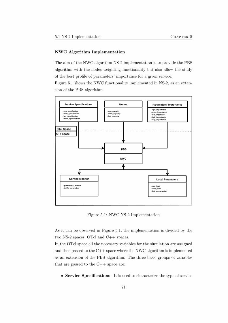
5.1 NS-2 Implementation Chapter 5
NWC Algorithm Implementation
The aim of the NWC algorithm NS-2 implementation is to provide the PBS
algorithm with the nodes weighting functionality but also allow the study
of the best profile of parameters’ importance for a given service.
Figure 5.1 shows the NWC functionality implemented in NS-2, as an exten-
sion of the PBS algorithm.
Service Requirements
OTcl Space
Service Specifications
- cpu_specification- mem_specification- bat_specification- traffic_specification
Service Requirements Nodes
- cpu_capacity- mem_capacity- bat_capacity
Service Requirements Parameters’ Importance
- cpu_importance- mem_importance- bat_importance- link_importance- deg_importance
C++ Space
Service Requirements PBS
NWC
Service Requirements Service Monitor
- parameters_monitor- traffic_generation
Service Requirements Local Parameters
- cpu_load- mem_load- bat_consumption
Figure 5.1: NWC NS-2 Implementation
As it can be observed in Figure 5.1, the implementation is divided by the
two NS-2 spaces, OTcl and C++ spaces.
In the OTcl space all the necessary variables for the simulation are assigned
and then passed to the C++ space where the NWC algorithm is implemented
as an extension of the PBS algorithm. The three basic groups of variables
that are passed to the C++ space are:
• Service Specifications - It is used to characterize the type of service
71

Chapter 5 Implementation
that is simulated. Variables representing CPU/memory load genera-
tion, battery consumption and also traffic (rate) between zone servers
and its clients are defined and passed to the PBS agent, in the C++
space, to be used in the service simulation.
• Nodes - Nodes’ local parameters capacity (CPU, memory and bat-
tery) which are used to simulate the CPU/memory load generation
and battery consumption, are assigned to every node of the network
that participates in the service deployment. This will allow the com-
putation of the parameters’ values for the node’s weight computation.
• Parameters’ Importance - Represent the importance values as-
signed to the different parameters of the NWC algorithm. When com-
puting the best profile these values are changed and the results of the
simulation are analyzed to select the most appropriate combination,
according to the simulated service and the objectives defined for the
selected DS.
In the C++ space some extensions to the PBS algorithm have also been
made. The basic NWC algorithm implementation has been included in the
PBS Agent. This node’s weight computation functionality is called by the
PBS algorithm each time an election takes place, as it presented in the FSM
in Appendix B.
In the C++ space the following functionality has been added:
• Service Monitor - This functionality is responsible for monitoring
and checking the local parameters values. It also controls the traffic
generation between zone servers and clients, which is performed ac-
cording the service specifications. This functionality is called at each
election time to update the parameters values for the node’s weight
computation. Periodically statistics about the parameters are taken
and the local parameters (CPU, memory and battery) values are check,
if they are not in the range of admissible values an anomaly is gener-
ated, this question is discussed in more detail in section 3.4.
72

5.1 NS-2 Implementation Chapter 5
• Local Parameters - This functionality is responsible for the gener-
ation of the local parameters values according to the node’s capacity
and the service characteristics.
In table 5.1 a summary of the file structure of the PBS algorithm with
the NWC algorithm extension is given. More details can be found in the
programming documentation in Siramon project webpage 2. In Appendix
C the steps for installation of the PBS/NWC algorithm are given.
PBS/NWC implementation in NS-2
File Description
zss{.h .cc} The main class for any ZSS implementation.
zss pbs{.h .cc} Implements the PBS/NWC algorithm sup-
port.
timer pbs{.h .cc} Timer functionality used by the PBS/NWC
algorithm.
neighborlist{.h .cc} Stores and handles the relevant information
about the neighbors.
node information.h Contains the structure of a node entry in
the Neighborlist and the structure of the sent
packets by the PBS algorithm.
monitor{.h .cc} Monitors the 1-hop neighborhood.
service monitor{.h .cc} Implements the service monitor functionality.
timer monitor{.h .cc} Timer functionality used by the monitor, and
the service monitor.
local parameters{.h .cc} Local parameter values generation.
debugger{.h .cc} Debugger used to write outputs.
utils/fsm{.h .cc} Implementation of a Finite State Machine
(FSM).
utils/state{.h .cc} State of the FSM.
Table 5.1: Files Used for PBS/NWC Implementation in NS-2
2www.siramon.org
73

Chapter 5 Implementation
5.2 Siramon Implementation
The implementation of the PBS algorithm in the Siramon framework fol-
lows the same approach of the NS-2 implementation, it is an extension of
the PBS algorithm, and this implementation is presented in this section.
Siramon is implemented in Java and has five basic modules:
• Service Specification
• Service Indication
• Service Deployment
• Service Management
• Environment Observer
A more detailed description of the Siramon framework is given in Appendix
D.
The NWC algorithm is implemented in three of the basic Siramon’s frame-
work modules: Service Specification, Service Management and Environment
Observed:
• Service Specification - This module is responsible for the service
description document definition and manipulation. This document is
written using the XML language [30]. To support the NWC functional-
ity the document has been extended with the profile of parameters’ im-
portance values (represented by the fields cpu i, mem i, bat i, link i and
deg i). This information is added under the DEMANDS element (path
SERVICE/IMPLEMENTATION/CODE/ENVIRONMENT/DEMANDS)
of the document. These fields are optional and will just be checked
if the service requires the zone server selection functionality. An ex-
tension on the specification module has also been made to allow the
extraction of the service profile.
74

5.2 Siramon Implementation Chapter 5
• Service Management - This module is responsible for the mainte-
nance, reconfiguration and termination of the services that use the
framework. Since the PBS algorithm is responsible for the selection
and maintenance of the zone servers, for a given service, it has been
implemented in this module. The NWC algorithm has also been imple-
mented in this module as an extension of the basic PBS algorithm. To
compute the node’s weight the necessary values of the parameters and
the parameters’ importance values are obtained using the specification
module and the Environment Observer module.
• Service Observer - The Environment Observer module has the func-
tionality of monitoring the device resources and the service context on
the network. To compute the node’s weight the NWC algorithm has
to monitor the CPU and memory load, the battery energy level and
the link quality of the connections to its neighbors. This functionality
has been included in this module. Four external monitors have been
created to monitor the four parameters, because Java does not have
native functionality to support the extraction of the required informa-
tion for the node’s weight computation.
Tables 5.2 and 5.3 give a resume of the file structure of the PBS algorithm
with the NWC algorithm extension in the Siramon framework. In Appendix
C some details about the implementation and the used external monitors
are given.
Package Description
Siramon.Management.zss Contains the main classes needed by
the ZSS functionality.
Siramon.Management.zss.utils Contains some utils for the ZSS
functionality like a basic debugger
and the Finite State Machine (FSM)
Table 5.2: Zone Server Selection Functionality in Siramon Framework
75

Chapter 5 Implementation
File Description
ZSS.java The main class for any ZSS implementation.
ZSS PBS.java Implements the PBS/NWC algorithm.
ZSS PBSfsm.java Implements the FSM used by the PBS/NWC
algorithm.
ZSS PBSpacket.java Used packet format to be sent in the content
part of the SIRAMON packet.
TimerPBS.java Timer functionality used by the PBS/NWC
algorithm.
Neighborlist.java Stores and handles the relevant information
about the neighbors.
NodeInformation Used by the Neighborlist to store the infor-
mation about a neighbor.
utils/Debugger.java Debugger used to write outputs.
utils/FSM.java Basic implementation of a Finite State Ma-
chine (FSM).
utils/State.java State of the FSM.
Table 5.3: Used Files for the PBS/NWC Implementation in SIRAMON
76

Chapter 6
Conclusions and Outlook
In this chapter conclusions about the achievements of this Master’s Thesis are
depicted and directions for further developments of the work are given.
6.1 Conclusions
New ways of communication are gaining popularity nowadays. MANETs are
one of these new trends, so new services and business areas are emerging for
these networks. To support such networks new protocols and functionality
are required to cope with the demanding and especially dynamic conditions
associated to it.
The support of distributed services deployment in MANETs has different
demands when compared to wired networks. The classical ”server-client”
and ”peer-to-peer” architectures are not well suited for the deployment of
distributed services in a MANET. New service management architectures
are being proposed for MANETs. An example of such architecture is the
Zone-based architecture [5]. It is a hybrid architecture that combines the
”good” features, in the MANETs context, of the two classical architectures.
This architecture is based on the notion of zone servers, which are special
network nodes that work as servers of a given network zone managing the
nodes that belong to its zone.
77
Chapter 6 Conclusions and Outlook
Previously an algorithm called PBS (Priority Based Selection) [6] has been
proposed for zone server selection and maintenance. PBS treats the network
as a graph and selects the DS based on node’s priorities. The first criterion
for the node’s priority assignment is the node’s weight, which measures the
capacity of a given node to perform as zone server for a given service.
Several algorithms exist to perform the selection of the DS nodes. The most
common approach for such selection is based on a small group of nodes’
characteristics aiming to optimize the DS selection for a unique objective.
In this thesis a different algorithm is proposed. The NWC (Node’s Weight
Computation) algorithm performs the selection of the most appropriate DS
as function of the service/system requirements. The algorithm, in conjunc-
tion with the PBS algorithm, allows the selection of DS nodes for non-specific
types of services, meaning that different objectives may be defined for the
DS selection. The algorithm is used in the Siramon framework [4] providing
the weighting functionality to the PBS algorithm to select the DS.
A group of parameters is taken into account to quantify the weight of the
network nodes, in total five parameters are used. The parameters are divided
into two classes, node’s processing/power parameters and node’s communi-
cation parameters. The first group contains the parameters which measure
the processing power capabilities of the nodes (CPU and memory) and the
energy capabilities of the nodes (battery). Concerning to communication
parameters the node’s degree and the link quality parameters are used, to
measure the communication capabilities of a node with its neighbors.
To use the algorithm in the deployment of different services, the notion of pa-
rameter importance level has been introduced. These importance values are
assigned to the parameters as function of the service/system requirements.
For example, if the service requires good connections and fast processing
nodes, the processing parameters (CPU and memory) and the link quality
parameter are assigned with a high importance value.
To allow the differentiation of the parameters’ importance a scale of three
values is used (no importance, normal importance and high importance), see
section 3.3.1 for more details.
78

6.1 Conclusions Chapter 6
The definition of the parameter importance values for a service, or service
profile, is made in a static way. This means that it is not adaptable to
the current service context. To study the most appropriate combination of
importance values for a given service a framework has been created, the
NWC framework.
The NWC framework allows, by performing a factorial design based on
the service properties, to study the contribution of each parameter in the
selection of the DS. To find the most appropriate profile a multi-objective
optimization technique is used. Such technique is used because a multiple
objectives are usually defined for the DS, such minimum number of DS
changes and minimum number of DS nodes.
The definition of the service profile may also be defined directly by the
service/system designer, according to the goals defined for the DS.
The NWC algorithm has been tested using simulation. A test service was
used modeling a real service (real time multiplayer game) characteristics.
It was simulated in two different scenarios. The NWC framework has been
used to evaluate and search for the best profile for the service. Good results
were obtained and it was clear that in all the simulated scenarios one profile
was the more appropriated, given the defined objectives for the DS.
Such conclusions confirmed that the proposed static assignment will be, in
general, consistent in the selection of the DS nodes for a given service, in
different conditions. This is mainly explained by the fact that a service is
characterized for a set of properties and characteristics that generate, even
in different contexts, a pattern behavior and this is reflected in the require-
ments for the DS selection.
The NWC algorithm has been implemented in the Siramon framework [4].
Given the constraints of the testbed, it could not be observed and studied
the importance of the use of the NWC algorithm in the selection of the DS
nodes. However it was observed that the more powerful nodes were selected
for the DS when the algorithm was used.
79

Chapter 6 Conclusions and Outlook
6.2 Outlook
From the performed work, some future lines of investigation and develop-
ment of the proposed algorithm are here depicted:
Different scenarios - During the performed evaluation of the algorithm
two different scenarios have been used. A random way point mobility
model was used in these simulation. To study the NWC algorithm
in more realistic conditions other scenarios should be also tested. An
example that is nowadays having some interest is the vehicular ad
hoc networks. Some simulation scenarios are being proposed for this
cases, for example an highway scenario where the movement of cars is
simulated in a high way. Such tests will allow to conclude about the
performance of the algorithm in more realistic scenarios.
Node’s weight computation formula - The NWC algorithm formula for
node’s weight computation follows a linear combination of the param-
eters values assigned with a given importance value. Every parameter
value is normalized into an unitary scale and the weight for a node is
then computed. Given the characteristics of the parameters and also
the importance that they have in the DS selection for a given service,
different combinations may conduct to a more appropriate selection of
the DS nodes. Some more research in the weight computation formula
should be done, studying different combinations of the parameters and
their importance values.
Testbed - The test and evaluation of an algorithm is usually performed
under simulation due to the complexity of construct a real test envi-
ronment. But it is impossible to transpose all service/scenario/system
properties for a simulation. It is suggested to test the NWC algo-
rithm in a real scenario, testbed. A representative testbed containing
a large number of different types of devices and reproducing real ser-
vice deployment situation will allow to perform measurements and
depict conclusions about the algorithm performance. This will allow
to study and develop the algorithm further.
80

Appendix A
Best Profile Computations
In this chapter the computation for the best profile using a multi-objective
optimization technique is performed.
A.1 Factorial Design Results
In this section the results of the performed factorial design are presented.
In Table A.1 the importance values, or profile, combinations to perform the
experimental design are presented. After, Tables A.2 and A.3 present the
results of the factorial design for the school yard scenario and test scenario,
respectively.
A.2 The Best Profile
There are five metrics that measure the performance of the system and the
objective is to minimize all these metrics, for the best profile computation.
Such a goal is not possible because some of the objectives cannot be optimize
at the same time.
To accomplish the optimization a multi-objective optimization technique is
going to be used. This is used in the computation of the best profile for the
service in both scenarios.
81

Appendix A Best Profile Computations
Importance Values Combinations
Combination CPU memory battery link quality degree
1 0.5 0.5 0 0.5 0.5
2 0.5 0.5 0 0.5 1
3 0.5 0.5 0 1 0.5
4 0.5 0.5 0 1 1
5 0.5 1 0 0.5 0.5
6 0.5 1 0 0.5 1
7 0.5 1 0 1 0.5
8 0.5 1 0 1 1
9 1 0.5 0 0.5 0.5
10 1 0.5 0 0.5 1
11 1 0.5 0 1 0.5
12 1 0.5 0 1 1
13 1 1 0 0.5 0.5
14 1 1 0 0.5 1
15 1 1 0 1 0.5
16 1 1 0 1 1
Table A.1: Parameters’ Importance Combinations for Factorial Design
A.2.1 Multi-Objective Optimization
A multi-objective problem consists of the search of the values for the design
variables which optimizes a set of objective functions. The set of variables
that produces the optimal outcome is designated as the optimal combination.
It yields a set of possible answers from which the designer may choose the
desired values of the design variables.
The usual approach in the search of the global optimization consists of
weighting the several objective functions, or decreasing the number of used
objective functions by setting constraints. In the following point a weighting
objectives method is presented.
82

A.2 The Best Profile Appendix A
School Yard Scenario
Combination DS nodes DS Changes Anomalies PKT loss Latency
1 3.98 2.14 0.71 0.30 6.94
2 3.82 2.57 0.86 0.25 6.82
3 3.98 1.71 0.71 0.34 6.91
4 3.88 1.86 0.71 0.23 6.77
5 3.80 2.29 0.86 0.28 6.82
6 3.71 2.43 1.00 0.25 6.84
7 4.05 2.86 1.29 0.27 6.86
8 3.77 2.43 0.86 0.29 6.88
9 4.19 2.43 0.86 0.25 6.88
10 3.98 1.57 0.57 0.30 6.77
11 3.95 1.57 0.71 0.36 6.85
12 4.01 2.00 0.86 0.30 6.89
13 3.87 1.43 0.43 0.35 6.75
14 3.77 1.43 0.57 0.36 6.85
15 3.96 1.71 0.57 0.36 6.84
16 3.77 1.43 0.57 0.36 6.83
Table A.2: Factorial Design Results - School Yard scenario
Weighting Objectives Method
This method takes each objective function and multiplies it by a ”weighting
coefficient”, which is represented by wi. The modified functions are then
added together to obtain a single cost function. The objective functions, fi,
must be optimized before the multi-objective optimization.
f(x) =k∑
i=1
wifi(x) (A.1)
where: 0 ≤ wi ≤ 1 and∑k
i=1 wi = 1
In this method the weighting coefficients are assumed beforehand. The
designer is expected to pick the values of the variables from this set of
solutions.
83

Appendix A Best Profile Computations
Test Scenario
Combination DS nodes DS Changes Anomalies PKT loss Latency
1 8.0079 5.7143 1.4286 1.3603 6.4327
2 8.4862 6.0 1.4286 1.0546 6.5939
3 8.1992 5.1429 0.8571 1.122 6.6504
4 8.4653 5.1429 1.1429 0.9305 6.5207
5 8.4902 5.7143 1.2857 1.176 6.5328
6 8.6763 5.1429 1.2857 1.2371 6.4607
7 8.4076 5.0 1.2857 1.3829 6.5003
8 8.3879 4.4286 1.0 1.0782 6.5117
9 8.2385 5.1429 1.2857 1.1768 6.5258
10 7.8952 5.8571 1.7143 1.0728 6.4482
11 8.0917 4.7143 1.1429 1.4099 6.5436
12 8.1953 5.8571 1.5714 1.3021 6.4536
13 8.2346 4.4286 0.8571 1.0735 6.4214
14 8.1009 4.5714 1.1429 1.0894 6.5254
15 8.3709 5.1429 1.0 1.2234 6.5112
16 8.4535 4.8571 0.8571 1.3612 6.5603
Table A.3: Factorial Design Results - Test scenario
A.2.2 Best Weight Profile Computation
In the designed experiment fi(x) represent the measured (mean) values of
the metrics used for the system evaluation:
• Number of DS Nodes
• Number of DS Changes
• Number of Anomalies
• Packet Loss
• Latency
From the performed study in 4.6.1, it has been concluded that packet loss
and latency metrics are not relevant in the evaluation of the system’s per-
84

A.2 The Best Profile Appendix A
formance. This happens because they show a constant behavior for all used
combinations of weight factors.
Hence, the multi-objective function will have three basic objectives:
• Minimize the Number of DS nodes
• Minimize the Number of DS changes
• Minimize the Number of Anomalies
As it has been presented, the global objective for the evaluated system is first
to guarantee a stable and robust DS selection and second to the best MDS
approximation. Based on such assumptions, the combinations of weights
presented in Table A.4 were used to find the best profile.
Objective Function Weight Factors
Metric Weight
Number of DS changes 5/10
Number of Anomalies 3/10
Number of DOMINATOR nodes 2/10
Table A.4: Objective Function Weights
In both scenarios, for each combination the defined multi-objective function
(MOF) can be then described as:
MOF = 2/10·Num Nodes+5/10·Num Changes+3/10·Num Anomalies
(A.2)
In the next sections the results of the MOF computation for all the param-
eters’ importance values combinations on the school yard scenario and test
scenario are presented. Before the computation of the MOF a normalization
of all the metrics into a unitary scale has been made.
A.2.3 School Yard Scenario
Table A.5 represents the MOF computations. It can be observed that the
best profile, minimal value of the MOF, occurs when the combination 13
85

Appendix A Best Profile Computations
is used. This combination has high importance assigned to CPU and mem-
ory parameters and normal importance assigned to link quality and degree
parameters.
School Yard MOF Computation
Combination Num Nodes Num Changes Num Anomalies MOF
1 0.56 0.50 0.33 0.52
2 0.23 0.80 0.50 0.60
3 0.57 0.20 0.33 0.31
4 0.35 0.30 0.33 0.32
5 0.19 0.60 0.50 0.49
6 0.00 0.70 0.67 0.55
7 0.70 1.00 1.00 0.94
8 0.11 0.70 0.50 0.52
9 1.00 0.70 0.50 0.70
10 0.55 0.10 0.17 0.21
11 0.49 0.10 0.33 0.25
12 0.61 0.40 0.50 0.47
13 0.32 0.00 0.00 0.06
14 0.13 0.00 0.17 0.08
15 0.52 0.20 0.17 0.25
16 0.13 0.00 0.17 0.08
Table A.5: MOF computation, School Yard Scenario
A.2.4 Test Scenario
Table A.6 represents the MOF computations for the test scenario experi-
mental design. It can be observed that the best profile is obtained, as in the
case of the school yard scenario, when combination 13 is used. This combi-
nation has high importance weight factor associated to CPU and memory,
and normal importance associated to link quality and degree parameters.
86

A.2 The Best Profile Appendix A
Test Scenario MOF Computation
Combination Num Nodes Num Changes Num Anomalies MOF
1 0.14 0.90 0.67 0.68
2 0.76 1.10 0.67 0.90
3 0.39 0.50 0.00 0.33
4 0.73 0.50 0.33 0.50
5 0.76 0.90 0.50 0.75
6 1.00 0.50 0.50 0.60
7 0.66 0.40 0.50 0.48
8 0.63 0.00 0.17 0.18
9 0.44 0.50 0.50 0.49
10 0.00 1.00 1.00 0.80
11 0.25 0.20 0.33 0.25
12 0.38 1.00 0.83 0.83
13 0.43 0.00 0.00 0.09
14 0.26 0.10 0.33 0.20
15 0.61 0.50 0.17 0.42
16 0.71 0.30 0.00 0.29
Table A.6: MOF computation, Test Scenario
87


Appendix B
Finite State Machine (FSM)
This chapter presents the Finite State Machine (FSM) used in the PBS al-
gorithm NS-2 and Siramon implementations. As the NWC algorithm is imple-
mented as an extension to the PBS algorithm, here an updated version of the
FSM is provided.
B.1 Introduction
A FSM is a model of behavior composed of states, transitions and actions.
Between different states of the machine some transitions are defined that
perform the defined actions based on incoming events. The specification of
the used FSM in the PBS/NWC algorithm implementation is shown in Fig.
B.1.
B.2 The States
The FSM consists of four states: ”idle”, ”msgsent”, ”roundfinished” and
”finished” state. The ”idle” state is the initial state of the FSM. PBS algo-
rithm performs in rounds. When the node goes off the initial state (”idle”)
and joins the service deployment, computes its weight and sends its neigh-
borslist, with the computed weight, to its neighbors. In every round it sends
89

Appendix B Finite State Machine (FSM)
Figure B.1: Finite State Machine (FSM)
the neighborlist to its neighbors and waits in the ”msgsent” state for the
neighborlists from the neighbors. If all required neighborlists have arrived,
or the timeout timer has expired, it goes to the ”roundfinished” state. In this
state it determines its own status based on the its weight and the informa-
tion available from the neighborhood. If there are still INT CANDIDATE
neighbors, the neighborlist is resent. At this point the FSM is again waiting
in the ”msgsent” state. If all INT CANDIDATE neighbors have switched
to DOMINATEE or DOMINATOR status, the FSM goes to the ”finished”
state. It is waiting in the ”finished” state unless there are some changes
in the network topology detected (some new INT CANDIDATE neighbors
arrive) or if some anomaly in the local parameters is observed. If this is the
case, a new round of the PBS algorithm will be started and the FSM returns
to the ”msgsent” state. In this transition the node computes its weight to
start a new election.
B.3 The Transitions and Actions
In Table B.1 shows all transitions/events and respective actions.
90

B.3 The Transitions and Actions Appendix B
From State To State Event Action
idle msgsent join Node joins the service, computes
node’s weight and starts sending out
neighborlists.
idle msgsent receivedmsg Node in idle state, but received a
neighborlist. Computes its weight and
starts sending out neighborlists.
msgsent msgsent timerRESEND Resend timer expired and not all
neighbors sent a neighborlist back. So,
the already sent neighborlist will be re-
sent.
msgsent roundfinished receivedmsg All required neighborlists have arrived.
Node determines its own status, based
on its weight and its neighbors weights.
msgsent roundfinished timerTIMEOUT Not all required neighborlists arrived,
but the timeout timer expired, so the
node determines its own status.
roundfinished msgsent resend There are still INT CANDIDATE
neighbors, a new round of PBS needs
to be started.
roundfinished finished finished All nodes determined their status, no
INT CANDIDATE neighbors left.
finished finished receivedmsg Handles incoming neighborlist. If re-
quired it sends a neighborlist back.
finished msgsent resend Anomaly in the local parameters,
changes in the network and/or some
INT CANDIDATE neighbors have
been detected. Computes node’s
weight and starts a new round of the
PBS/NWC.
Table B.1: Transitions of the Finite State Machine (FSM) for PBS/NWC.
91


Appendix C
NWC algorithm NS-2
Installation
In this chapter a tutorial for installation of the implemented functionality in
NS-2 is given.
C.1 Installation
The following steps have to be taken, to install NS-2 and the PBS/NWC
functionality:
1. Download the Ns-Allinone package from the official NS-2 homepage
and install it according to the instructions.
2. Copy the zoneserver directory containing the implementation into the
ns-2 main directory (e.g., ns-allinone-2.29/ns-2.29).
3. Some changes in some of the ns source files are required to add the
new agent, especially because a new packet format is used:
• Add to the file ’common/packet.h’ the new packet protocol ID
’PT ZSS’ to the second last line of the ’enum packet t {}’. In
the same file you have to add the line ’name [PT ZSS]=”zss”;’
to the ’p info()’ function and the line ’double snr ;’ to the ’struct
hdr cmn’, to support the SNR monitoring functionality.
93

Appendix C NWC algorithm NS-2 Installation
• The file ’tcl/lib/ns-default.tcl’ has to be edited, too. This is the
file where all default values for the Tcl objects are defined. Insert
the line ’Agent/ZSS set weight 0’ to set the default weight for
Agent/ZSS.
• The new packet has also to be added in the file ’tcl/lib/ns-
packet.tcl’ in the ’foreach prot’ loop with the entry ’ZSS’.
• Add the following code to the ’mac/mac-802 11.cc’ file, in the
’recv(Packet *p, Handler *h)’ function:
double snr;
if(rx_state_ == MAC_IDLE) {
snr = 10*log10(p->txinfo_.RxPr) -10;
} else {
snr = 10*log10(p->txinfo_.RxPr/pktRx_->txinfo_.RxPr) - 10;
}
hdr->snr_ = snr;
• The last change is a change that has to be applied to the ’Make-
file’. All sourcefiles has to be added after the ’OBJ CC=’ list:
zoneserver/zss.o zoneserver/zss pbs.o zoneserver/debugger.o
zoneserver/timer pbs.o zoneserver/timer monitor.o
zoneserver/monitor.o zoneserver/neighborlist.o
zoneserver/utils/fsm.o zoneserver/utils/state.o
zoneserver/link process.o zoneserver/local parameters.o
zoneserver/service monitor.o.
4. Recompile ns by using make clean; make depend; make.
5. After recompilation the Tcl scripts can be used to run simulations with
the command ns example.tcl.
94

Appendix D
Siramon Framework
In this chapter a brief description of the Siramon framework is given.
D.1 Introduction
SIRAMON [4] (Service provIsioning fRAMework for self-Organized Net-
works) is a generic, decentralized and modular service provisioning frame-
work for self organized networks. It integrates all the required service provi-
sioning functionality to support the whole life-cycle of a service, integrating
service specification, advertisement/lookup, deployment, management and
environment monitoring mechanisms.
SIRAMON structure consists of five different modules. Each module has
different functionality, but they cooperate with each other to give a complete
service provisioning framework to the application layer services.
Figure D.1 represents the SIRAMON structure.
D.2 The Structure
Next, a brief description of each of the modules is given:
Service Specification - Defines a universal service description language
to describe the services that will be supported by the framework. XML
95

Appendix D Siramon Framework
Figure D.1: SIRAMON architecture
Information Set [30] is used for the service description. The services
are defined in a tree structure based on the type of service. The
description is included in a XML document that is handled by the
framework to allow the support of it.
Service Indication - It is responsible for advertisement and service lookup
procedures on the network. Due the lack of a central infrastructure
this procedures are completely distributed.
Service Deployment - This functionality includes all the necessary steps
for the deployment of a service. It may have several operations asso-
ciated:
• Requesting/Downloading software.
• Discovering/Gathering resources.
• Mapping the service specifications to the resources.
• Configuring the resources and installing/configuring the service
software.
96

D.2 The Structure Appendix D
• Activating the service, synchronized with the other service par-
ticipants.
• Handling the control on the management module.
Service Management - Service Management contains all the functional-
ity of service maintenance, reconfiguration and termination functions
of the running services.
• The service maintenance keeps track on the service context,
adapting dynamically the service to its context (resource vari-
ations, new nodes) in order to optimize user’s perceived service
quality hiding all the scenario conditions changes to the node.
• The service reconfiguration is responsible for the reconfiguration
of the service, globally or locally. Local reconfiguration is trans-
parent to the other users. It happens when the context of the
device changes or the service user intends to modify the running
service session. When global reconfiguration happens, all the
service users will perceive the change and a global reconfigura-
tion/synchronization occurs.
• The service termination can be seen as a special case of ser-
vice reconfiguration, when a device stops running its service in-
stance. This occurrence is informed to all other participants, the
resources have to be released and the participant nodes will then
reconfigure their service instances to the new service scenario.
Environment Observer - This module is responsible for monitoring the
device resources and the service context on the network. It collects in-
formation about the context of the service locally/globally and trans-
forms it into an appropriate form to be used as input for the deploy-
ment and management modules.
Siramon is a platform-independent framework, which is an imperative re-
quirement due the heterogeneity associated to MANETs. To achieve this
independence it is written in Java.
97

Appendix D Siramon Framework
For more details about the Siramon framework [4] should be consulted.
98

Appendix E
Used Abbreviations
ad hoc for this (latin); for a particular case without any form of centralized
administration.
DS Dominating Set ; A dominating set of a graph, is a subset of nodes such
that all nodes are neighbor of a node in the DS or are itself in the DS.
FSM Finite State Machine; A FSM is a model of behavior composed of
states, transitions and actions.
MAC Medium Access Control ; Handles access to a shared medium.
MANET Mobile Ad hoc Network ; Temporary network in which devices
want to communicate with each other, with a continuously changing
network topology and without any form of centralized administration.
MANET is also the name of an IETF working group, that is working
in the field of ad hoc networks.
MDS Minimum Dominating Set ; A Dominating Set (DS) is called a MDS
if the number of nodes in the DS is minimal.
NS-2 Network Simulator 2 ; NS-2 is a discrete event driven simulator to
support networking research.
OTcl MIT Object Tcl ; An extension to Tcl/Tk for object-oriented pro-
gramming.
99

Appendix E Used Abbreviations
P2P Peer-to-peer ; Network that does not have fixed clients and servers,
but a number of peer nodes that function as both clients and servers
to the other nodes on the network. Any node is able to initiate or
complete any supported transaction.
PBS Priority Based Selection; An algorithm that selects the Zone Servers
supporting a zone-based architecture based on comparing priorities of
the nodes.
SIRAMON Service Provisioning Framework for Mobile Ad-hoc Networks;
A proposal of a generic, decentralized service provisioning framework
for mobile ad hoc networks [2].
WLAN Wireless Local Area Network ; In a WLAN the device (e.g. a lap-
top, PDA, etc.) communicates via a wireless connection with a WLAN
Access Point which is connected (just like a normal computer) via a
cable to the Internet or the local network. As the devices are not
wired up the users are mobile. This is the advantage of a WLAN. The
indoor range depends on structural factors and is considerably lower
than outdoors, where WLAN connections are possible over more than
200 metres.
XML Extensible Markup Language; Simple, very flexible text format for
electronic publishing and data exchanging, standardised by the World
Wide Web Consortium (W3C).
ZSS Zone Server Selection; The selection procedure for choosing the Zone
Servers supporting a zone-based architecture.
100

Bibliography
[1] Mobile Entertainement Industry and Culture (mGain). Mobile Enter-
tainment in Europe: Current state of Art.
[2] K. Farkas, O. Wellnitz, M. Dick, X. Gu, M. Busse, W. Effelsberg,
Y.Rebahi, D. Sisalem, D. Grigoras, K. Stefanidis and D. N. Serpanos.
Real-time Service Provisioning for Mobile and Wireless Networks. Else-
vier Computer Communications journal., 29(5):540–550, March 2005.
[3] S. Helal, N. Desai, V. Verma, and C. Lee. Konark - a service discovery
and delivery protocol for ad-hoc networks, 2003.
[4] K. Farkas. SIRAMON - Service provIsioning fRAMework for self-
Organized Networks. ETH Zurich, January 2005.
http://www.csg.ethz.ch/research/projects/siramon/.
[5] S.M. Riera, O. Wellnitz, and L. Wolf. A Zone-based Gaming Architec-
ture for Ad-Hoc Networks. In Proceedings of the Workshop on Network
and System Support for Games (NetGames2003), Redwood City, USA,
May 2003.
[6] F. Maurer. Service Management Procedures Supporting Distributed
Services in Mobile Ad Hoc Networks, 31st August 2005. MA-2005-14.
[7] Information Sciences Institute ISI. The Network Simulator ns-2.
http://www.isi.edu/nsnam/ns/.
[8] GNU.org. The GNU General Public License.
http://www.gnu.org/licenses/licenses.html#TOCGPL.
101

Appendix BIBLIOGRAPHY
[9] E. Cronin, B. Filstrup, and A. Kurc. A distributed multiplayer game
server system, 2001.
[10] R. Wattenhofer. Chapter 8 - Dominating Sets. Course material mobile
computing, Distributed Computing Group, ETH Zurich, 2004.
[11] L. Jia, R. Rajaraman, and T. Suel. An efficient distributed algorithm for
constructing small dominating sets. Distributed Computing, 15(4):193–
205, December 2002.
[12] J. Wu and H. Li. Handbook of wireless networks and mobile computing,
chapter A Dominating-Set-Based Routing Scheme in Ad Hoc Wireless
Networks, pages 425–450. 2003. ISBN:0-471-41902-8.
[13] F. Kuhn and R. Wattenhofer. Constant-Time Distributed Dominating
Set Approximation. In Proceedings of the 22nd ACM Symposium on
Principles of Distributed Computing (PODC’03), pages 25–32, Boston,
Massachusetts, USA, July 2003.
[14] K. M. Alzoubi, P-J. Wan, and O. Frieder. Message-optimal Connected
Dominating Sets in Mobile Ad Hoc Networks. In Proceedings of the
3rd ACM International Symposium on Mobile Ad Hoc Networking &
Computing 2002, pages 157–164, Lausanne, Switzerland, June 2002.
[15] D. Dubhashi, A. Mei, A. Panconesi, J. Radhakrishnan, and A. Srini-
vasan. Fast Distributed Algorithms for (Weakly) Connected Dominat-
ing Sets and Linear-Size Skeletons. In Proceedings of the 14th Annual
ACM-SIAM Symposium on Discrete Algorithms 2003, pages 717–724,
Baltimore, Maryland, USA, January 2003.
[16] P. Klein and R. Ravi. A nearly best-possible approximation algorithm
for node-weighted steiner trees. Journal of Algorithms, 19:104–115,
1995.
[17] M. Gerla and J. Tsai. Multicluster, mobile, multimedia radio network.
Journal of Wireless Networks, 1(3):255–265, 1995.
[18] A.K. Pareh. Selecting routers in ad-hoc wireless networks.
102

BIBLIOGRAPHY Appendix
[19] D.J Baker and A. Ephremides. A Distributed algorithm for Organizing
Mobile Radio Telecommunication Networks. In Proceedings of the 2nd
International Conference in Distributed Computer Systems, 1981.
[20] Ivan Stojmenovic Jie Wu Jamil A. Shaikh, Julio Solano. New Metrics
for Dominating Set Based Energy Efficient Activity Scheduling in Ad
Hoc Networks. In 28th Annual IEEE International Conference on Local
Computer Networks (LCN’03), 2003.
[21] M. Chatterjee, S. Das, and D. Turgut. WCA: A weighted clustering
algorithm for mobile ad hoc networks. In Journal of Cluster Computing
(Special Issue on Mobile Ad hoc Networks), vol. 5, pp. 193–204., 2002.
[22] T. Hossmann. Mobility Prediction in Mobile Ad Hoc Networks, 30th
April 2006. MA-2006-08.
[23] Raj Jain. The Art of Computer Systems Performance Analysis. John
Wiley Sons, Inc., 1991.
[24] Nathan Sheldon, Eric Girard, Seth Borg, Mark Claypool, and Em-
manuel Agu. The Effect of Latency on User Performance in Warcraft
III. In NETGAMES ’03: Proceedings Workshop on Network and Sys-
tem Support for Games, May 2003.
[25] Tom Beigbeder, Rory Coughlan, Corey Lusher, John Plunkett, Em-
manuel Agu, and Mark Claypool. The Effects of Loss and Latency on
User Performance in Unreal Tournament 2003. In Proceedings Work-
shop on Network and System Support for Games, pages 144–151, Au-
gust 2004.
[26] Broch, J. and Maltz, D. A. and Johnson, D. B. and Hu, Y-C. and
Jetcheva, J. A Performance Comparison of Multi-Hop Wireless Ad
Hoc Network Routing Protocols. In Proceedings of ACM/IEEE Inter-
national Conference on Mobile Computing and Networking (MobiCom),
pages 85–97, October 1998.
[27] T. S. Rappaport. Wireless Communications, Principles and Practice.
Prentice Hall International, 1996.
103

Appendix BIBLIOGRAPHY
[28] T. Camp, J. Boleng, and V. Davies. A Survey of Mobility Models for Ad
Hoc Network Research. Wireless Communications & Mobile Comput-
ing (WCMC): Special issue on Mobile Ad Hoc Networking: Research,
Trends and Applications, 2(5):483–502, 2002.
[29] Q. Zheng, X. Hong, and S. Ray. Recent Advances in Mobility Modeling
for Mobile Ad Hoc Network Research. In ACM-SE 42: Proceedings of
the 42nd annual Southeast regional conference, pages 70–75, New York,
NY, USA, 2004. ACM Press.
[30] World Wide Web Consortium (W3C). XML Information Set.
104