hybrid propulsion system of a long endurance electric uav · hybrid propulsion system of a long...
TRANSCRIPT
Hybrid Propulsion System of a Long Endurance ElectricUAV
Tiago Miguel Moreira Ferreira
Thesis to obtain the Master of Science Degree in
Mechanical Engineering
Supervisor(s): Prof. André Calado Marta
Prof. Virginia Isabel Monteiro Nabais Infante
Examination Committee
Chairperson: Prof. Luís Manuel Varejão Oliveira Faria
Supervisor: Prof. André Calado Marta
Member of the Committee: Prof. António Manuel Relógio Ribeiro
November 2014

ii

Acknowledgments
I would like to thank my parents, Gracinda Ferreira and Mario Ferreira, for supporting me along my
academic path. I would also like to thank Daniela Carvalho for always being there to help me along the
way.
Thanks to the professors, Dr. Andre Marta and Dr. Virginia Infante, that guided me and helped me
during the making of this thesis. And also thanks Diogo Rechena for the help in spell checking and proof
reading.
iii

iv
Resumo
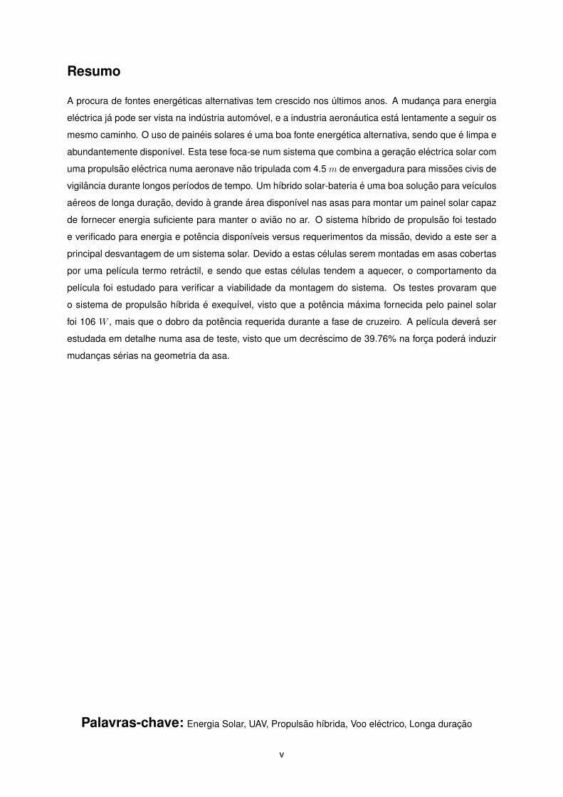
A procura de fontes energeticas alternativas tem crescido nos ultimos anos. A mudanca para energia
electrica ja pode ser vista na industria automovel, e a industria aeronautica esta lentamente a seguir os
mesmo caminho. O uso de paineis solares e uma boa fonte energetica alternativa, sendo que e limpa e
abundantemente disponıvel. Esta tese foca-se num sistema que combina a geracao electrica solar com
uma propulsao electrica numa aeronave nao tripulada com 4.5 m de envergadura para missoes civis de
vigilancia durante longos perıodos de tempo. Um hıbrido solar-bateria e uma boa solucao para veıculos
aereos de longa duracao, devido a grande area disponıvel nas asas para montar um painel solar capaz
de fornecer energia suficiente para manter o aviao no ar. O sistema hıbrido de propulsao foi testado
e verificado para energia e potencia disponıveis versus requerimentos da missao, devido a este ser a
principal desvantagem de um sistema solar. Devido a estas celulas serem montadas em asas cobertas
por uma pelıcula termo retractil, e sendo que estas celulas tendem a aquecer, o comportamento da
pelıcula foi estudado para verificar a viabilidade da montagem do sistema. Os testes provaram que
o sistema de propulsao hıbrida e exequıvel, visto que a potencia maxima fornecida pelo painel solar
foi 106 W , mais que o dobro da potencia requerida durante a fase de cruzeiro. A pelıcula devera ser
estudada em detalhe numa asa de teste, visto que um decrescimo de 39.76% na forca podera induzir
mudancas serias na geometria da asa.
Palavras-chave: Energia Solar, UAV, Propulsao hıbrida, Voo electrico, Longa duracao
v

vi
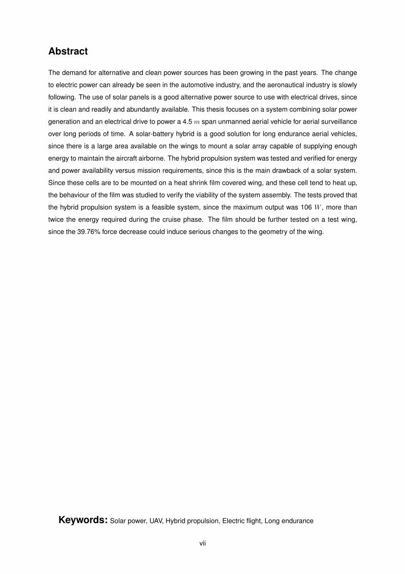
Abstract
The demand for alternative and clean power sources has been growing in the past years. The change
to electric power can already be seen in the automotive industry, and the aeronautical industry is slowly
following. The use of solar panels is a good alternative power source to use with electrical drives, since
it is clean and readily and abundantly available. This thesis focuses on a system combining solar power
generation and an electrical drive to power a 4.5 m span unmanned aerial vehicle for aerial surveillance
over long periods of time. A solar-battery hybrid is a good solution for long endurance aerial vehicles,
since there is a large area available on the wings to mount a solar array capable of supplying enough
energy to maintain the aircraft airborne. The hybrid propulsion system was tested and verified for energy
and power availability versus mission requirements, since this is the main drawback of a solar system.
Since these cells are to be mounted on a heat shrink film covered wing, and these cell tend to heat up,
the behaviour of the film was studied to verify the viability of the system assembly. The tests proved that
the hybrid propulsion system is a feasible system, since the maximum output was 106 W , more than
twice the energy required during the cruise phase. The film should be further tested on a test wing,
since the 39.76% force decrease could induce serious changes to the geometry of the wing.
Keywords: Solar power, UAV, Hybrid propulsion, Electric flight, Long endurance
vii

viii

Contents
Acknowledgments . . . . . . . . . . . . . . . . . . . . . . . . . . . . . . . . . . . . . . . . . . . iii
Resumo . . . . . . . . . . . . . . . . . . . . . . . . . . . . . . . . . . . . . . . . . . . . . . . . . v
Abstract . . . . . . . . . . . . . . . . . . . . . . . . . . . . . . . . . . . . . . . . . . . . . . . . . vii
List of Tables . . . . . . . . . . . . . . . . . . . . . . . . . . . . . . . . . . . . . . . . . . . . . . xiii
List of Figures . . . . . . . . . . . . . . . . . . . . . . . . . . . . . . . . . . . . . . . . . . . . . xvii
Nomenclature . . . . . . . . . . . . . . . . . . . . . . . . . . . . . . . . . . . . . . . . . . . . . . xix
Glossary . . . . . . . . . . . . . . . . . . . . . . . . . . . . . . . . . . . . . . . . . . . . . . . . xxii
1 Introduction 1
1.1 Motivation . . . . . . . . . . . . . . . . . . . . . . . . . . . . . . . . . . . . . . . . . . . . . 1
1.2 About this thesis . . . . . . . . . . . . . . . . . . . . . . . . . . . . . . . . . . . . . . . . . 2
1.3 Structure of the document . . . . . . . . . . . . . . . . . . . . . . . . . . . . . . . . . . . . 2
2 Solar Power 3
2.1 A Journey to Photovoltaics . . . . . . . . . . . . . . . . . . . . . . . . . . . . . . . . . . . 3
2.2 Solar Power Alternatives . . . . . . . . . . . . . . . . . . . . . . . . . . . . . . . . . . . . . 4
2.3 Solar Flight . . . . . . . . . . . . . . . . . . . . . . . . . . . . . . . . . . . . . . . . . . . . 5
2.3.1 History of Solar Powered Flight . . . . . . . . . . . . . . . . . . . . . . . . . . . . . 6
2.3.2 High Altitude Long Endurance Flights . . . . . . . . . . . . . . . . . . . . . . . . . 7
2.3.3 Piloted Solar Flight . . . . . . . . . . . . . . . . . . . . . . . . . . . . . . . . . . . . 10
3 Aircraft, Mission and Hybrid Propulsion 13
3.1 Mission . . . . . . . . . . . . . . . . . . . . . . . . . . . . . . . . . . . . . . . . . . . . . . 13
3.2 Aircraft . . . . . . . . . . . . . . . . . . . . . . . . . . . . . . . . . . . . . . . . . . . . . . . 14
3.3 Hybrid Propulsion . . . . . . . . . . . . . . . . . . . . . . . . . . . . . . . . . . . . . . . . 17
4 Solar Cells 19
4.1 Introduction . . . . . . . . . . . . . . . . . . . . . . . . . . . . . . . . . . . . . . . . . . . . 19
4.2 Solar Cell Design . . . . . . . . . . . . . . . . . . . . . . . . . . . . . . . . . . . . . . . . . 19
4.3 Solar Cell Testing . . . . . . . . . . . . . . . . . . . . . . . . . . . . . . . . . . . . . . . . . 21
4.3.1 Indoor Testing . . . . . . . . . . . . . . . . . . . . . . . . . . . . . . . . . . . . . . 21
4.3.2 Outdoor Testing . . . . . . . . . . . . . . . . . . . . . . . . . . . . . . . . . . . . . 22
ix
4.3.3 Testing Method Selection . . . . . . . . . . . . . . . . . . . . . . . . . . . . . . . . 22
4.4 Pyranometer . . . . . . . . . . . . . . . . . . . . . . . . . . . . . . . . . . . . . . . . . . . 22
4.4.1 PV Cell Pyranometer . . . . . . . . . . . . . . . . . . . . . . . . . . . . . . . . . . . 22
4.4.2 Silicon-Cell Photodiode Pyranometer . . . . . . . . . . . . . . . . . . . . . . . . . . 22
4.4.3 Thermopile Pyranometer . . . . . . . . . . . . . . . . . . . . . . . . . . . . . . . . 23
4.5 MPPT . . . . . . . . . . . . . . . . . . . . . . . . . . . . . . . . . . . . . . . . . . . . . . . 24
5 Energy Accumulator 27
5.1 Mechanical Accumulator . . . . . . . . . . . . . . . . . . . . . . . . . . . . . . . . . . . . . 27
5.2 Electrical Accumulator . . . . . . . . . . . . . . . . . . . . . . . . . . . . . . . . . . . . . . 28
5.3 Chemical Accumulator . . . . . . . . . . . . . . . . . . . . . . . . . . . . . . . . . . . . . . 28
6 Sensors and Data Acquisition System 31
6.1 Electrical Parameters Sensors . . . . . . . . . . . . . . . . . . . . . . . . . . . . . . . . . 31
6.2 Load Sensor . . . . . . . . . . . . . . . . . . . . . . . . . . . . . . . . . . . . . . . . . . . 32
6.3 Temperature Sensor . . . . . . . . . . . . . . . . . . . . . . . . . . . . . . . . . . . . . . . 33
7 Material Research and Selection 35
7.1 Solar Cell . . . . . . . . . . . . . . . . . . . . . . . . . . . . . . . . . . . . . . . . . . . . . 35
7.2 MPPT . . . . . . . . . . . . . . . . . . . . . . . . . . . . . . . . . . . . . . . . . . . . . . . 36
7.3 Energy Accumulator . . . . . . . . . . . . . . . . . . . . . . . . . . . . . . . . . . . . . . . 36
7.4 Pyranometer . . . . . . . . . . . . . . . . . . . . . . . . . . . . . . . . . . . . . . . . . . . 36
7.5 Electrical Sensors . . . . . . . . . . . . . . . . . . . . . . . . . . . . . . . . . . . . . . . . 38
7.6 Load Sensors . . . . . . . . . . . . . . . . . . . . . . . . . . . . . . . . . . . . . . . . . . . 39
7.7 Temperature Sensors . . . . . . . . . . . . . . . . . . . . . . . . . . . . . . . . . . . . . . 40
8 Sub Systems Testing 41
8.1 Electrical Sensor Calibration . . . . . . . . . . . . . . . . . . . . . . . . . . . . . . . . . . 41
8.2 Solar Cells . . . . . . . . . . . . . . . . . . . . . . . . . . . . . . . . . . . . . . . . . . . . 43
8.2.1 Test Design . . . . . . . . . . . . . . . . . . . . . . . . . . . . . . . . . . . . . . . . 43
8.2.2 Single Cell Testing . . . . . . . . . . . . . . . . . . . . . . . . . . . . . . . . . . . . 45
8.2.3 Efficiency Loss from Film Covering . . . . . . . . . . . . . . . . . . . . . . . . . . . 48
8.2.4 Efficiency Gains from Changing the Incidence Angle . . . . . . . . . . . . . . . . . 49
8.2.5 Multiple Cells Testing . . . . . . . . . . . . . . . . . . . . . . . . . . . . . . . . . . 50
8.3 Full Array . . . . . . . . . . . . . . . . . . . . . . . . . . . . . . . . . . . . . . . . . . . . . 52
8.3.1 Cell Storage Design . . . . . . . . . . . . . . . . . . . . . . . . . . . . . . . . . . . 52
8.3.2 Full Array Test . . . . . . . . . . . . . . . . . . . . . . . . . . . . . . . . . . . . . . 53
8.4 MPPT Solar Charger Testing . . . . . . . . . . . . . . . . . . . . . . . . . . . . . . . . . . 54
8.4.1 Test Design . . . . . . . . . . . . . . . . . . . . . . . . . . . . . . . . . . . . . . . . 54
8.4.2 MPPT Testing . . . . . . . . . . . . . . . . . . . . . . . . . . . . . . . . . . . . . . . 54
8.5 Electric Motor Testing . . . . . . . . . . . . . . . . . . . . . . . . . . . . . . . . . . . . . . 55
x
8.5.1 Testing Apparatus . . . . . . . . . . . . . . . . . . . . . . . . . . . . . . . . . . . . 55
8.5.2 Motor Testing . . . . . . . . . . . . . . . . . . . . . . . . . . . . . . . . . . . . . . . 56
9 Complete Hybrid Propulsion System 61
9.1 Complete System Hardware . . . . . . . . . . . . . . . . . . . . . . . . . . . . . . . . . . . 61
9.2 Hybrid Propulsion System Testing . . . . . . . . . . . . . . . . . . . . . . . . . . . . . . . 61
9.3 Mission Simulation . . . . . . . . . . . . . . . . . . . . . . . . . . . . . . . . . . . . . . . . 64
10 Heat Shrink Film Test 69
10.1 Testing Apparatus . . . . . . . . . . . . . . . . . . . . . . . . . . . . . . . . . . . . . . . . 69
10.2 Experimental Results . . . . . . . . . . . . . . . . . . . . . . . . . . . . . . . . . . . . . . 74
11 Conclusions 77
11.1 Achievements . . . . . . . . . . . . . . . . . . . . . . . . . . . . . . . . . . . . . . . . . . . 77
11.2 Future Work . . . . . . . . . . . . . . . . . . . . . . . . . . . . . . . . . . . . . . . . . . . . 79
Bibliography 84
A Equipment Technical Sheet 85
xi

xii
List of Tables
3.1 Relevant dimensions of the designed aircraft. . . . . . . . . . . . . . . . . . . . . . . . . . 15
3.2 Summarized estimated performance of the designed aircraft. . . . . . . . . . . . . . . . . 15
4.1 Wavelength sensitivity. . . . . . . . . . . . . . . . . . . . . . . . . . . . . . . . . . . . . . . 20
5.1 Typical specific energy of several battery technologies [Epec, 2014]. . . . . . . . . . . . . 29
7.1 Pyranometers and sub systems found during market research. . . . . . . . . . . . . . . . 37
7.2 Electrical sensors found during market research. . . . . . . . . . . . . . . . . . . . . . . . 39
8.1 Screenshots of the developed LabView program. . . . . . . . . . . . . . . . . . . . . . . . 42
8.2 Results of the voltage and current sensors testing for calibration. . . . . . . . . . . . . . . 43
8.3 Multiple PV cell test. . . . . . . . . . . . . . . . . . . . . . . . . . . . . . . . . . . . . . . . 45
8.4 Resistors used in the single solar cell testing. . . . . . . . . . . . . . . . . . . . . . . . . . 47
8.5 Results of the film variation experiment. . . . . . . . . . . . . . . . . . . . . . . . . . . . . 49
8.6 Results of the tilt variation experiment. . . . . . . . . . . . . . . . . . . . . . . . . . . . . . 50
8.7 Resistances used in the three solar cell connected in parallel testing. . . . . . . . . . . . . 51
8.8 Full array tests. . . . . . . . . . . . . . . . . . . . . . . . . . . . . . . . . . . . . . . . . . . 53
8.9 MPPT tests. . . . . . . . . . . . . . . . . . . . . . . . . . . . . . . . . . . . . . . . . . . . . 55
8.10 Aerodynamic forces during the different phases of the flight [Vidales, 2013]. . . . . . . . . 56
8.11 Power use for the different propellers to fulfil the thrust requirements. . . . . . . . . . . . . 60
xiii

xiv
List of Figures
2.1 Odeillo solar furnace [Odeillo, 2014b]. . . . . . . . . . . . . . . . . . . . . . . . . . . . . . 5
2.2 Solar One thermal solar power plant in California [EERE, 2014]. . . . . . . . . . . . . . . 5
2.3 World record setting solar powered model aeroplanes. . . . . . . . . . . . . . . . . . . . . 6
2.4 Noteworthy solar powered model aeroplanes. . . . . . . . . . . . . . . . . . . . . . . . . . 7
2.5 NASA Pathfinder [Pathfinder]. . . . . . . . . . . . . . . . . . . . . . . . . . . . . . . . . . . 7
2.6 NASA Centurion [Centurion]. . . . . . . . . . . . . . . . . . . . . . . . . . . . . . . . . . . 8
2.7 NASA Helios [Helios]. . . . . . . . . . . . . . . . . . . . . . . . . . . . . . . . . . . . . . . 9
2.8 NASA ERAST project evolution [Noll et al., 2004]. . . . . . . . . . . . . . . . . . . . . . . 9
2.9 Solitair, with its unique pivoting solar panels [DLR, 2014]. . . . . . . . . . . . . . . . . . . 9
2.10 QinetiQ Zephyr in flight [Zephyr, 2014]. . . . . . . . . . . . . . . . . . . . . . . . . . . . . . 10
2.11 Gossamer Penguin [Noth, July 2008]. . . . . . . . . . . . . . . . . . . . . . . . . . . . . . 10
2.12 Solar Impulse 1 [SolarImpulse1, 2014]. . . . . . . . . . . . . . . . . . . . . . . . . . . . . 11
3.1 Graphical representation of the LEEUAV mission. . . . . . . . . . . . . . . . . . . . . . . . 14
3.2 LEEUAV aerofoil geometry obtained. . . . . . . . . . . . . . . . . . . . . . . . . . . . . . . 15
3.3 Some results of the parametric study using the energy model. . . . . . . . . . . . . . . . . 15
3.4 Rendering of the CAD concept. . . . . . . . . . . . . . . . . . . . . . . . . . . . . . . . . . 16
3.5 Three view drawing of the concept aircraft with its main dimensions. . . . . . . . . . . . . 16
3.6 Scheme of the hybrid propulsion system for the LEEUAV . . . . . . . . . . . . . . . . . . . 17
4.1 International Space Station with solar panels [NASA, 2014]. . . . . . . . . . . . . . . . . . 19
4.2 Workings of a basic solar cell [Olympus, 2014]. . . . . . . . . . . . . . . . . . . . . . . . . 20
4.3 Solar spectrum at sea level on a clear day. . . . . . . . . . . . . . . . . . . . . . . . . . . . 21
4.4 Photovoltaic cell pyranometer [Soldata, 2014]. . . . . . . . . . . . . . . . . . . . . . . . . 23
4.5 Silicon-cell photodiode pyranometer [Apogee, 2014]. . . . . . . . . . . . . . . . . . . . . . 23
4.6 Thermopile pyranometer constitution [GlobalSpec, 2014]. . . . . . . . . . . . . . . . . . . 24
4.7 Thermopile pyranometer [EKO, 2014]. . . . . . . . . . . . . . . . . . . . . . . . . . . . . . 24
4.8 Tipical I-V curve for the C60 SunPower PV cell [SunPower]. . . . . . . . . . . . . . . . . 24
5.1 Flywheel schematics [Physics, 2014]. . . . . . . . . . . . . . . . . . . . . . . . . . . . . . 27
5.2 Capacitor schematics [TEWN]. . . . . . . . . . . . . . . . . . . . . . . . . . . . . . . . . . 28
5.3 Hyperion G3 VX 3S LiPo battery . . . . . . . . . . . . . . . . . . . . . . . . . . . . . . . . 29
xv
6.1 Nationals Instruments NI PCIe-6321 [Instruments, 2014]. . . . . . . . . . . . . . . . . . . 31
6.2 Hall effect sensor schematics [Racz, 2012]. . . . . . . . . . . . . . . . . . . . . . . . . . . 32
6.3 Strain gauge schematics . . . . . . . . . . . . . . . . . . . . . . . . . . . . . . . . . . . . . 33
7.1 SunPower C60 PV cell [SunPower, 2014] . . . . . . . . . . . . . . . . . . . . . . . . . . . 35
7.2 Five by two PV cells panel [Vidales, 2013] . . . . . . . . . . . . . . . . . . . . . . . . . . . 35
7.3 Genasun’s GV-10 Lithium [Genasun, 2014]. . . . . . . . . . . . . . . . . . . . . . . . . . . 36
7.4 Vishay Model STC S-Type load lell [Vishay]. . . . . . . . . . . . . . . . . . . . . . . . . . . 40
7.5 Thermometers used in the tests. . . . . . . . . . . . . . . . . . . . . . . . . . . . . . . . . 40
8.1 Voltage calibration test of one of the sensors. . . . . . . . . . . . . . . . . . . . . . . . . . 42
8.2 Current calibration test of one of the sensors. . . . . . . . . . . . . . . . . . . . . . . . . . 43
8.3 Tipical I-V for the C60 SunPower pv cell [SunPower]. . . . . . . . . . . . . . . . . . . . . 44
8.4 Single solar cell testing. . . . . . . . . . . . . . . . . . . . . . . . . . . . . . . . . . . . . . 44
8.5 Solar irradiation measuring system. . . . . . . . . . . . . . . . . . . . . . . . . . . . . . . 46
8.6 Times of the single cell tests and evolution of the solar irradiation during the day. . . . . . 46
8.7 Single cell test. . . . . . . . . . . . . . . . . . . . . . . . . . . . . . . . . . . . . . . . . . . 47
8.8 Evolution of the power output. . . . . . . . . . . . . . . . . . . . . . . . . . . . . . . . . . . 48
8.9 Test of the single PV cell with film covering. . . . . . . . . . . . . . . . . . . . . . . . . . . 48
8.10 Test of the single cell with variation to the incidence angle. . . . . . . . . . . . . . . . . . . 49
8.11 Circuit assembly used for the multiple cell tests. . . . . . . . . . . . . . . . . . . . . . . . . 50
8.12 Test with three cells connected in series. . . . . . . . . . . . . . . . . . . . . . . . . . . . . 51
8.13 Test with 3 cells connected in parallel. . . . . . . . . . . . . . . . . . . . . . . . . . . . . . 51
8.14 Single cell and the two circuits converted to single cell power. . . . . . . . . . . . . . . . . 52
8.15 Solar array transportation and storage crate. . . . . . . . . . . . . . . . . . . . . . . . . . 53
8.16 Full panel testing using light bulbs for load and a power meter for parameter measuring. . 54
8.17 Testing of the complete power supply of the hybrid system. . . . . . . . . . . . . . . . . . 54
8.18 Final apparatus for motor testing. . . . . . . . . . . . . . . . . . . . . . . . . . . . . . . . . 57
8.19 Weights for use in the load cell calibration. . . . . . . . . . . . . . . . . . . . . . . . . . . . 57
8.20 Load cell calibration and linear regression result. . . . . . . . . . . . . . . . . . . . . . . . 57
8.21 Propellers used in the motor test. . . . . . . . . . . . . . . . . . . . . . . . . . . . . . . . . 58
8.22 Thrust output by power consumed. . . . . . . . . . . . . . . . . . . . . . . . . . . . . . . . 58
8.23 Thrust output versus the rotational speed of the propeller. . . . . . . . . . . . . . . . . . . 59
8.24 Power per Newton of thrust output versus the rotational speed of the propeller. . . . . . . 60
9.1 Schematic of the complete hybrid propulsion system. . . . . . . . . . . . . . . . . . . . . . 61
9.2 Assembly of the full hybrid system used in its testing. . . . . . . . . . . . . . . . . . . . . . 62
9.3 Power output of the battery and MPPT during the hybrid propulsion system test. . . . . . 62
9.4 Power required during the mission and power available from the solar array during the
summer [Marta and Gamboa, 2014]. . . . . . . . . . . . . . . . . . . . . . . . . . . . . . . 63
xvi
9.5 Power required during the mission and power available from the solar array during the
winter [Marta and Gamboa, 2014]. . . . . . . . . . . . . . . . . . . . . . . . . . . . . . . . 63
9.6 Current and voltage output of the MPPT during the hybrid propulsion system test. . . . . 64
9.7 Hybrid propulsion system assembly for the full mission simulation. . . . . . . . . . . . . . 65
9.8 Power required by the motor and power supplied by the energy generation sub-system
during the full hybrid propulsion system mission simulation test. . . . . . . . . . . . . . . . 65
9.9 Hybrid propulsion system assembly for the full mission simulation. . . . . . . . . . . . . . 66
9.10 Current and voltage during the climb phase of the mission simulation. . . . . . . . . . . . 66
9.11 Solar irradiance and energy generation sub-system power output during mission simulation. 67
9.12 Energy generation sub-system power output, efficiency and temperature of the solar array
during mission simulation. . . . . . . . . . . . . . . . . . . . . . . . . . . . . . . . . . . . . 67
10.1 Fist design of the film testing apparatus. . . . . . . . . . . . . . . . . . . . . . . . . . . . . 70
10.2 Final geometry of the film testing apparatus. . . . . . . . . . . . . . . . . . . . . . . . . . . 71
10.3 Final geometry of the aluminium load cell. . . . . . . . . . . . . . . . . . . . . . . . . . . . 71
10.4 Load test of the aluminium load cell. . . . . . . . . . . . . . . . . . . . . . . . . . . . . . . 72
10.5 Built aluminium load cell with the strain gauge. . . . . . . . . . . . . . . . . . . . . . . . . 72
10.6 Heating element used in the heat shrink film test. . . . . . . . . . . . . . . . . . . . . . . . 73
10.7 Strain indicator and dummy bridge used in the heat shrink film test. . . . . . . . . . . . . . 74
10.8 Heat shrink film test montage. . . . . . . . . . . . . . . . . . . . . . . . . . . . . . . . . . . 74
10.9 Test to validate the linearity of the aluminium load cell. . . . . . . . . . . . . . . . . . . . . 75
10.10Heat shrink film load tests with the thermocouple. . . . . . . . . . . . . . . . . . . . . . . . 75
10.11Heat shrink film load tests normalized so that the constant behaviour is evident . . . . . . 76
xvii

xviii

Nomenclature
Greek symbols
ηMPPT Efficiency of the Maximum Power Point Tracker (MPPT).
µε Micro Extension.
σ Tensile stress.
σallowed Maximum tensile stress allowed on the part.
ε Extension.
Roman symbols
A Current.
AM Measured Current.
Ealuminium Modulus of elasticity (or Young’s Modulus) for 2024 aluminium.
F Applied force.
IIn Current entering a node on a electrical circuit.
IOut Current exiting a node on a electrical circuit.
V Voltage.
VM Measured voltage.
VO Output voltage.
Vt Total voltage drop on a closed loop electrical circuit.
W Power.
xix

xx
Glossary
3D Aeromodelism flight class consisting of high al-
pha manoeuvres and tight turns pattern flying.
BLDC Brushless Direct Current electric motors.
CAD Computer Aided Designed used in the develop-
ment phase of new products.
ERAST Environmental Research Aircraft and Sensor
Technology.
F5B Aeromodelism class of high powered electric
gliders.
F5D Aeromodelism class of high speed flying race.
FPV First Person View, where the pilot fly the aero-
model by seeing a live feed from a on board
camera.
HALE High Altitude Long Endurance.
LCD Liquid Crystal Display.
LEEUAV Long Endurance Electric Unmanned Aerial Ve-
hicle.
LiFe Lithium iron phosphate battery.
LiPo Lithium Ion battery on a flexible polymer enclo-
sure.
MPPT Maximum Power Point Tracker used to maxi-
mize the power output of a solar array.
NASA National Aeronautics and Space Administra-
tion.
NiCd Nickel–Cadmium battery.
NiMh Nickel–Metal Hydride battery.
OSD On Screen Display.
PV Cell Solar photovoltaic cell.
RTB Return To Base.
UAV Unmanned Aerial Vehicle.
xxi

xxii
Chapter 1
Introduction
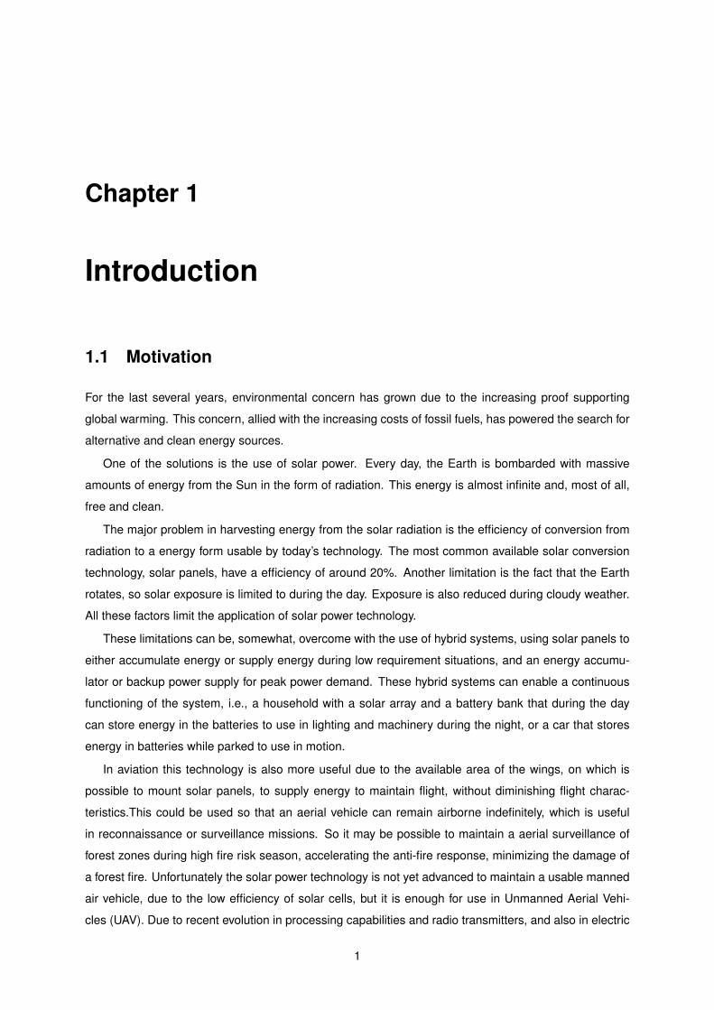
1.1 Motivation
For the last several years, environmental concern has grown due to the increasing proof supporting
global warming. This concern, allied with the increasing costs of fossil fuels, has powered the search for
alternative and clean energy sources.
One of the solutions is the use of solar power. Every day, the Earth is bombarded with massive
amounts of energy from the Sun in the form of radiation. This energy is almost infinite and, most of all,
free and clean.
The major problem in harvesting energy from the solar radiation is the efficiency of conversion from
radiation to a energy form usable by today’s technology. The most common available solar conversion
technology, solar panels, have a efficiency of around 20%. Another limitation is the fact that the Earth
rotates, so solar exposure is limited to during the day. Exposure is also reduced during cloudy weather.
All these factors limit the application of solar power technology.
These limitations can be, somewhat, overcome with the use of hybrid systems, using solar panels to
either accumulate energy or supply energy during low requirement situations, and an energy accumu-
lator or backup power supply for peak power demand. These hybrid systems can enable a continuous
functioning of the system, i.e., a household with a solar array and a battery bank that during the day
can store energy in the batteries to use in lighting and machinery during the night, or a car that stores
energy in batteries while parked to use in motion.
In aviation this technology is also more useful due to the available area of the wings, on which is
possible to mount solar panels, to supply energy to maintain flight, without diminishing flight charac-
teristics.This could be used so that an aerial vehicle can remain airborne indefinitely, which is useful
in reconnaissance or surveillance missions. So it may be possible to maintain a aerial surveillance of
forest zones during high fire risk season, accelerating the anti-fire response, minimizing the damage of
a forest fire. Unfortunately the solar power technology is not yet advanced to maintain a usable manned
air vehicle, due to the low efficiency of solar cells, but it is enough for use in Unmanned Aerial Vehi-
cles (UAV). Due to recent evolution in processing capabilities and radio transmitters, and also in electric
1
power and accumulation, UAVs are becoming more and more affordable and accessible. This makes
the development of early warning and surveillance aerial systems a plausible reality.
1.2 About this thesis
As the title ”Hybrid Propulsion of a Long Endurance Electric UAV” indicates, this thesis will focus on the
hybrid aspect of the propulsion a long endurance unmanned aerial vehicle. The UAV is being developed
for the LEEUAV project [Marta and Gamboa, 2014], and this thesis is a continuation of the Hector Vidalez
MsC thesis [Vidales, 2013]. On this project, the hybrid system has to be able to sustain a 8 hours flight,
including take off and climb to an altitude of 1000 m. To achieve this result, the solar array, the energy
accumulation and the whole hybrid system will be chosen and characterised to determine its capabilities.
So several parameters of the energy supply and management systems, and the power requirement of
the electric drive will be studied.
At the end of this project, the hybrid system must be able to supply enough energy to the power
system, so that the mission can be accomplished.
Another aspect to be studied is the effect the heat from the solar array will have on the wing structure,
which will be comprised of balsa and composite formers covered with a heat shrinking film, being that
the main focus will be the effect of the heat in the covering film.
1.3 Structure of the document
In this document, a brief introduction will be made concerning the history of UAV and solar power,
followed by the characterization of flight and power requirements during each phase of the mission. It
then continues to describe the hybrid portion of the system, the functioning of solar cells, the choice of
the energy accumulation system and the characterization of the hybrid system as a whole. This system
will then be characterized using a method described in the testing section.
After characterizing the hybrid system, the power system will be briefly tested, using a developed
simple testing device, to approximately determine the energy available in each phase of the mission.
Due to the type of construction used in the UAV, some problems can arise from the conjunctions with
the solar cells, so the assembly will be tested using a developed apparatus.
In the end, it should be possible to access the feasibility of the planned UAV mission by comparing
the available to the required energy in each mission phase.
2
Chapter 2
Solar Power
2.1 A Journey to Photovoltaics
Solar power has been harnessed by humans since the beginning of time, be it by building houses with
south facing windows to enjoy solar heat to bring warmth and comfort, or focusing solar rays to light
up torches, or even defend whole cities, as in the Archimedes story of the defence of Syracuse, where
he, allegedly set wooden boats afire by reflecting and concentrating solar rays using polished bronze
shields. Another example of early solar power harvesting is the hot box invented by Horace de Saussure
in 1767, in which a box could be used to harness solar heat, making it possible to cook using only power
from the Sun [EERE, 2014].
In 1876, the production of electricity by a material exposed to light is first observed in selenium by
Williams Grylls Adams and his student, Richard Evans Day. Although the current generated was not
enough to power electrical devices, this discovery marked the beginning of the solar directly generated
electricity [EERE, 2014, Perlin].
After this discovery, some advances were made in the characterization of the photovoltaic effect
and the manufacture of single crystal silicon by Jan Czochralski in 1918 [EERE, 2014], but the most
significant advance came from the Bell Laboratories in 1953, when Gerald Pearson inadvertently made
a silicon solar cell far more efficient than the selenium made solar cells. This first cell was then refined
and improved by Daryl Chapin and Calvin Fuller, and, by 1954, the Bell Laboratories had built a 4%
efficiency cell, which, in less than 18 months, jumped to 11% efficiency [EERE, 2014, Perlin].
Despite the advances in solar cells technology, the commercial breakthrough came from the space
race in the late 1950’s, when Dr. Hans Ziegler convinced the US Navy to install solar panels to power
the radio equipment aboard the Vanguard satellite. While initially refused because solar panels were
deemed untried technology, the US Navy accepted to incorporate solar panels, but with a chemical
battery backup. As Dr. Ziegler predicted, the chemical battery ran out within a week and the solar
panels continued to power the Vanguard for years. Although many scientists remained sceptical of the
use of solar panels to power bigger and harder ventures, solar engineers proved them wrong by building
bigger and more powerful solar arrays. This marked the beginning of the staple of using solar panels
3
to power space electrical equipment. Without solar cells, the telecommunications revolution might have
never occurred! [EERE, 2014, Perlin]
Despite the success of solar power in space applications, where the efficiency and durability out-
weighed the cost, its price was still too high for terrestrial usage. It was not until the early 1970’s, when
Dr. Elliot Berman, sponsored by the Exxon Corporation, built a solar cell with poorer grade silicon and
cheaper packaging materials,that the price of the solar cell became cost effective, lowering from $100 to
$20 per Watt, making this solution a bargain for electrical needs in locations far away from the grid, such
as oil rigs, navigation lights, rail road crossings and light houses. The profit from its low maintenance
and durability far outweighed the cost [EERE, 2014, Perlin].
In the 1970’s, with the oil price rises, most governments started to look for alternative power sources.
Some looked at nuclear power as the solution, but many looked at solar and wind energy as the alter-
native, due to the growth of the environmental conciousness. After the investment in this power source
in the late 1970’s and 1980’s, this new energy source was intended to follow the same plan as fossil
fuels, a centralized large power plant, which then transmitted its power to where it was needed. But, as
a solar panel can be fabricated to tailor each need, many engineers began to believe the best approach
would be that each building had its own solar panel to fulfil its energy need. This would reduce most of
the costs of a central solar plant, as the acquisition of land and the construction of the power distribution
lines. Due to this new way of thinking governments started to offer financial incentives for home owners
to install such systems to power their houses [Perlin].
As the price for solar cells continues to drop, solar power will continue to grow its participation in
energy production, and will start to be applied in different areas, such as transportation, becoming
the main and most cost effective power source in low power requirement applications, like emergency
phones in highways, and remote places where the distribution from the main power plant is either too
costly or too difficult to implement.
2.2 Solar Power Alternatives
In Sec. 2.1 the history of the direct electricity production by photovoltaic cells from solar radiation was
discussed, but solar power has alternative ways of being harvested, as the heat from solar radiation can
also be used. The simpler way is to build solar passive housing, in which the Sun is used for lightning
of the house and for temperature management. Although this is a intuitive idea, the first passive solar
house can be traced to the end of World War I in the Ruhr area [Jones and Bouamane, 2012].
Another way of using solar power is to convert its heat into electricity. This can be accomplished
by capturing the solar rays, and using them to heat up water enough to power a conventional turbine,
much like a conventional thermal power plant. For this purpose, a solar thermal power plant consists
on a central tower that captures the light from an array of mirrors that concentrate the Sun rays onto it.
The tower then uses these concentrated rays to heat water above its boiling point, which then powers a
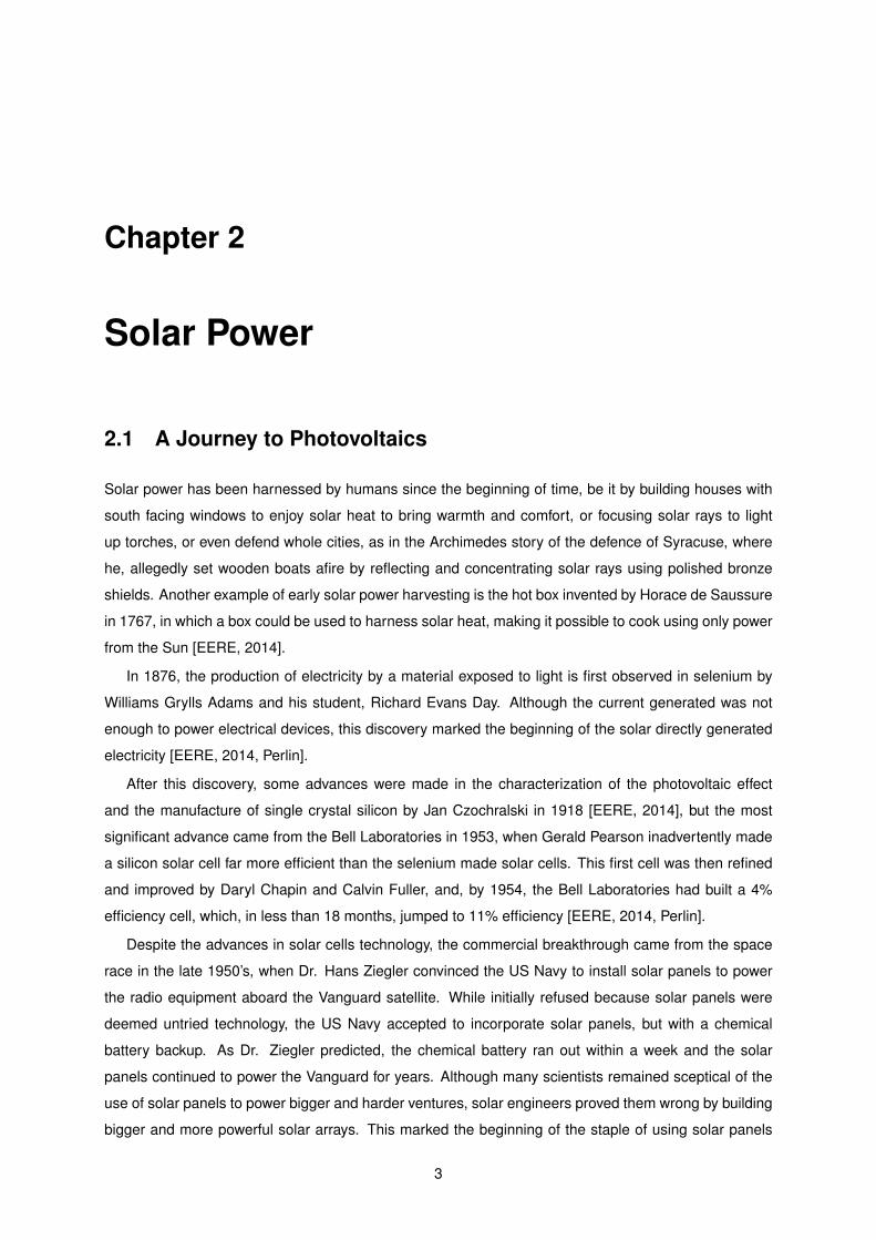
steam turbine. In 1969, France builds the Odeillo solar furnace [Fig. 2.1], in the Pyrenees mountains,
using an eight-story high stack of about 10,000 mirrors that focused the Sun light onto a hemisphere,
4
that could reach temperature up to 3,500oC. This heat would then be used to produce electricity and
high temperature metallurgic experiments [Odeillo, 2014a, EERE, 2014]
Figure 2.1: Odeillo solar furnace [Odeillo, 2014b].
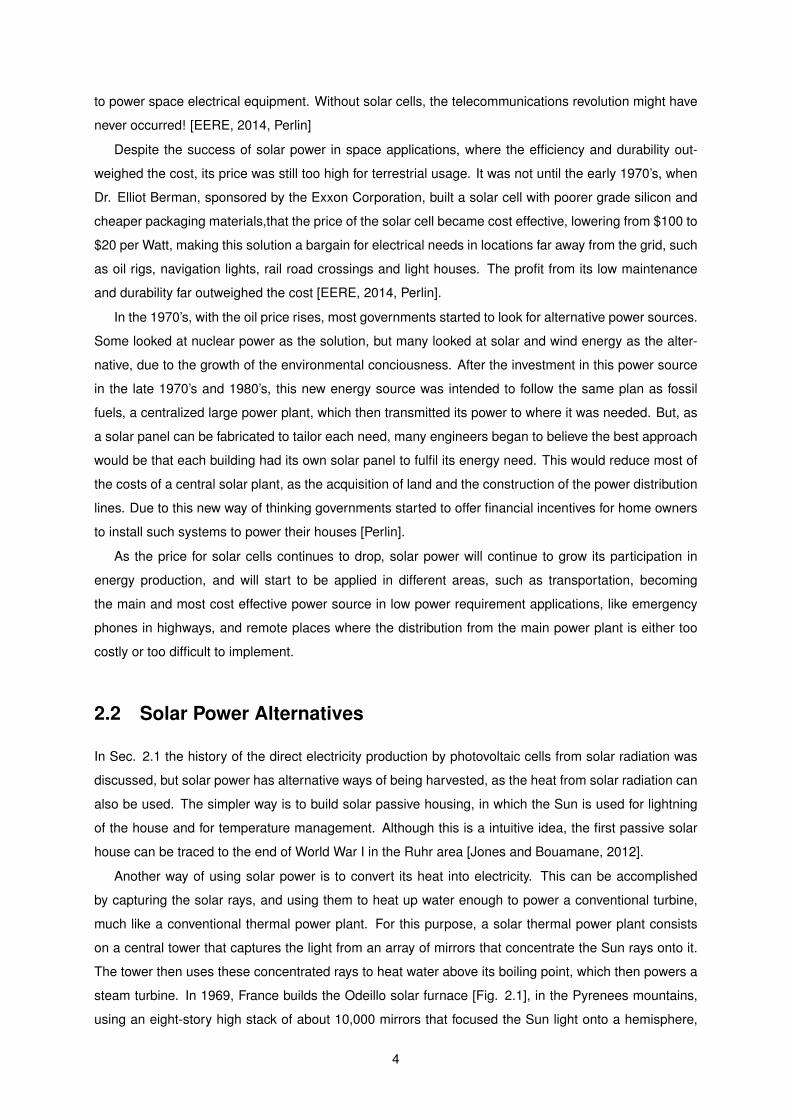
Later, in 1982, the U.S. Department of Energy, along with an industrial consortium, started to operate
Solar One [Fig. 2.2], a ten megawatt central receiver solar plant, comprised of computer controlled sun
tracking mirrors (heliostats) that focus solar radiation onto a receiver on top of a central tower, as a
demonstration of the functionality of this design. The receiver heats a heat transfer fluid, usually a salt,
which is then used to power a high efficiency steam turbine. This salt can also be stored and used when
it is difficult to obtain energy from the Sun, enabling the power plant to run 24 hours a day. At the end of
the project, Solar One could be dispatched 96% of the time, proving the validity of this concept [EERE,
2014].
Figure 2.2: Solar One thermal solar power plant in California [EERE, 2014].
Although very useful, these designs have the problem of only harvesting direct sunlight, ignoring
diffuse, light from clouds, and reflected sunlight.
2.3 Solar Flight
The first aircraft to use electric power was a hydrogen-filled dirigible, the France, during a 10 km race
around Villacoulbay and Medon, in 1884. At this time, the only rival to electric propulsion was the steam
engine, which was inferior to electric motor. But with the arrival of the internal combustion engine, the
field of electric power was abandoned for almost a century [Boucher, 1984].
The first recorded electric powered flight happened on the 30th of June 1957, when Colonel H. J.
Taplin flew his 2 m span model ”Radio Queen”, using a permanent magnet motor and a silver-zync
5
battery. Further developments came from Fred Militky, a german pioneer, that achieved his first electric
flight using a free flight model in October 1957 [Noth, July 2008]. The electric powered flight continued
to evolve, with improvements in the motors used, with the introduction of highly efficient electronic con-
trolled brushless motors, and improvements in batteries, with the upgrade to high energy density lithium
polymer batteries.
2.3.1 History of Solar Powered Flight
On the 4th of November 1974 Sunrise I took to the skies above a dry lake at Camp Irwin. This was the
first time a solar powered aircraft flew. The aircraft, designed by R. J. Boucher from Astro Flight Inc.,
flew for 20 minutes at an altitude of around 100 m. It had a wingspan of 9.76 m, a take-off weight of
12.25 kg and was powered by 4,096 solar cells, with a power output of 450 W [Boucher, 1984]. Later
an improved version was built, the Sunrise II, which had the same wingspan, but was lighter, at 10.21
kg, and had more power from its 4,480 solar cells, producing 600 W . The solar flight history had begun.
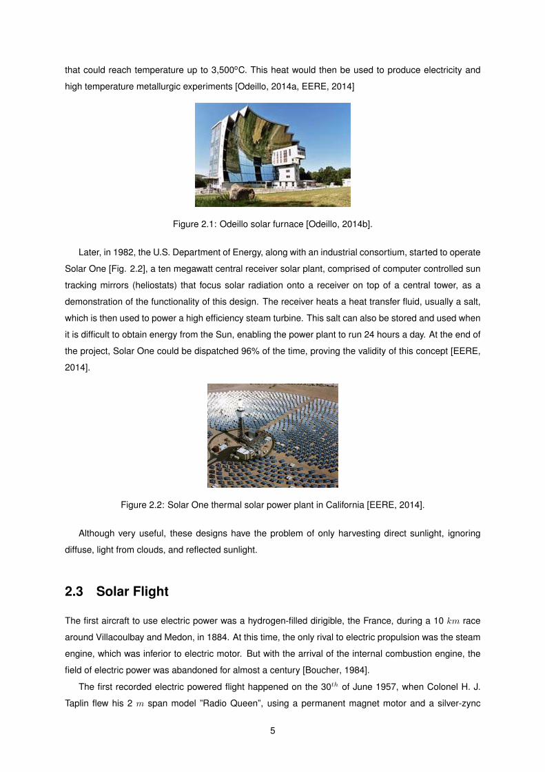
On August of 1996, Dave Beck, from Wisconsin, distinguished himself by setting the record for the
longest straight line flight in the model aeroplane solar category F5 open SOL, when his Solar Solitude
(Fig. 2.3(a)) flew 38.84 km, and reaching an altitude of 1,283 m two years later [Boucher, 1984]. From
1990 to 1999, these records were shattered by Wolfgang Schaeper with his Solar Excel (Fig. 2.3(b)),
eventually achieving the following records: longest flight duration (11h34m18s), longest distance in a
straight line (48.21 km), highest speed on a solar powered model aircraft (80.63 km/h), highest altitude
gain (2,065 m), highest speed on a closed circuit (62.15 km/h) and longest distance on a closed circuit
(190 km). These records have yet to be beaten, although some have been retired due to sporting rules
changes [FAI, 2014, Shaeper].
(a) Dave Beck’s Solar Soli-tude [Noth, July 2008].
(b) Wolfgang Schaeper’s Solar Excel [Excel, 1990].
Figure 2.3: World record setting solar powered model aeroplanes.
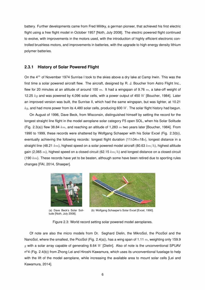
Of note are also the micro models from Dr. Seghard Dielin, the MikroSol, the PicoSol and the
NanoSol, where the smallest, the PicoSol (Fig. 2.4(a)), has a wing span of 1.11 m, weighting only 159.9
g with a solar array capable of generating 8.64 W [Dielin]. Also of note is the unconventional SPUAV
no4 (Fig. 2.4(b)) from Zhong Lei and Hiroshi Kawamura, which uses its unconventional fuselage to help
with the lift of the model aeroplane, while increasing the available area to mount solar cells [Lei and
Kawamura, 2014].
6
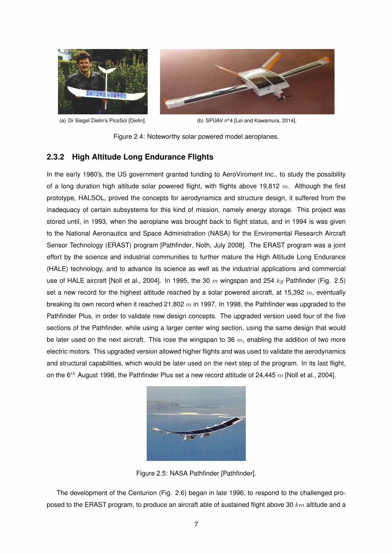
(a) Dr Siegel Dielin’s PicoSol [Dielin]. (b) SPUAV no4 [Lei and Kawamura, 2014].
Figure 2.4: Noteworthy solar powered model aeroplanes.
2.3.2 High Altitude Long Endurance Flights
In the early 1980’s, the US government granted funding to AeroViroment Inc., to study the possibility
of a long duration high altitude solar powered flight, with flights above 19,812 m. Although the first
prototype, HALSOL, proved the concepts for aerodynamics and structure design, it suffered from the
inadequacy of certain subsystems for this kind of mission, namely energy storage. This project was
stored until, in 1993, when the aeroplane was brought back to flight status, and in 1994 is was given
to the National Aeronautics and Space Administration (NASA) for the Enviromental Research Aircraft
Sensor Technology (ERAST) program [Pathfinder, Noth, July 2008]. The ERAST program was a joint
effort by the science and industrial communities to further mature the High Altitude Long Endurance
(HALE) technology, and to advance its science as well as the industrial applications and commercial
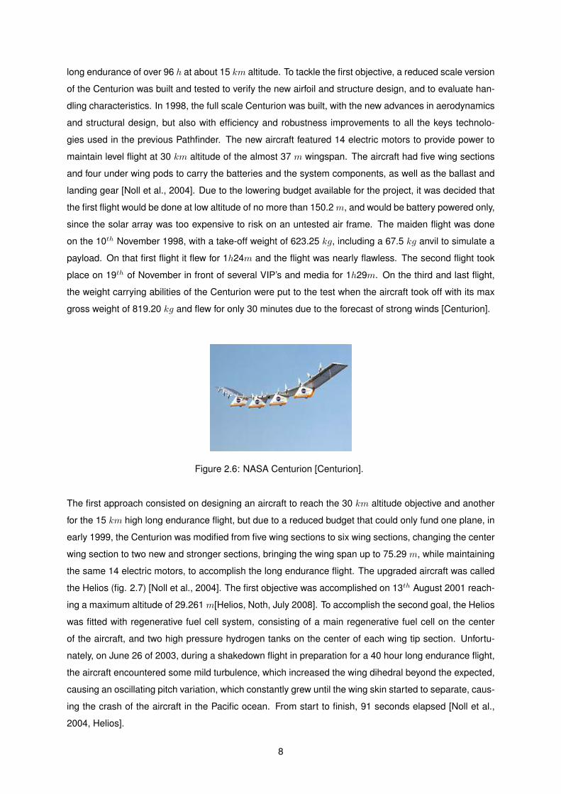
use of HALE aircraft [Noll et al., 2004]. In 1995, the 30 m wingspan and 254 kg Pathfinder (Fig. 2.5)
set a new record for the highest altitude reached by a solar powered aircraft, at 15,392 m, eventually
breaking its own record when it reached 21,802 m in 1997. In 1998, the Pathfinder was upgraded to the
Pathfinder Plus, in order to validate new design concepts. The upgraded version used four of the five
sections of the Pathfinder, while using a larger center wing section, using the same design that would
be later used on the next aircraft. This rose the wingspan to 36 m, enabling the addition of two more
electric motors. This upgraded version allowed higher flights and was used to validate the aerodynamics
and structural capabilities, which would be later used on the next step of the program. In its last flight,
on the 6th August 1998, the Pathfinder Plus set a new record altitude of 24,445 m [Noll et al., 2004].
Figure 2.5: NASA Pathfinder [Pathfinder].
The development of the Centurion (Fig. 2.6) began in late 1996, to respond to the challenged pro-
posed to the ERAST program, to produce an aircraft able of sustained flight above 30 km altitude and a
7
long endurance of over 96 h at about 15 km altitude. To tackle the first objective, a reduced scale version
of the Centurion was built and tested to verify the new airfoil and structure design, and to evaluate han-
dling characteristics. In 1998, the full scale Centurion was built, with the new advances in aerodynamics
and structural design, but also with efficiency and robustness improvements to all the keys technolo-
gies used in the previous Pathfinder. The new aircraft featured 14 electric motors to provide power to
maintain level flight at 30 km altitude of the almost 37 m wingspan. The aircraft had five wing sections
and four under wing pods to carry the batteries and the system components, as well as the ballast and
landing gear [Noll et al., 2004]. Due to the lowering budget available for the project, it was decided that
the first flight would be done at low altitude of no more than 150.2 m, and would be battery powered only,
since the solar array was too expensive to risk on an untested air frame. The maiden flight was done
on the 10th November 1998, with a take-off weight of 623.25 kg, including a 67.5 kg anvil to simulate a
payload. On that first flight it flew for 1h24m and the flight was nearly flawless. The second flight took
place on 19th of November in front of several VIP’s and media for 1h29m. On the third and last flight,
the weight carrying abilities of the Centurion were put to the test when the aircraft took off with its max
gross weight of 819.20 kg and flew for only 30 minutes due to the forecast of strong winds [Centurion].
Figure 2.6: NASA Centurion [Centurion].
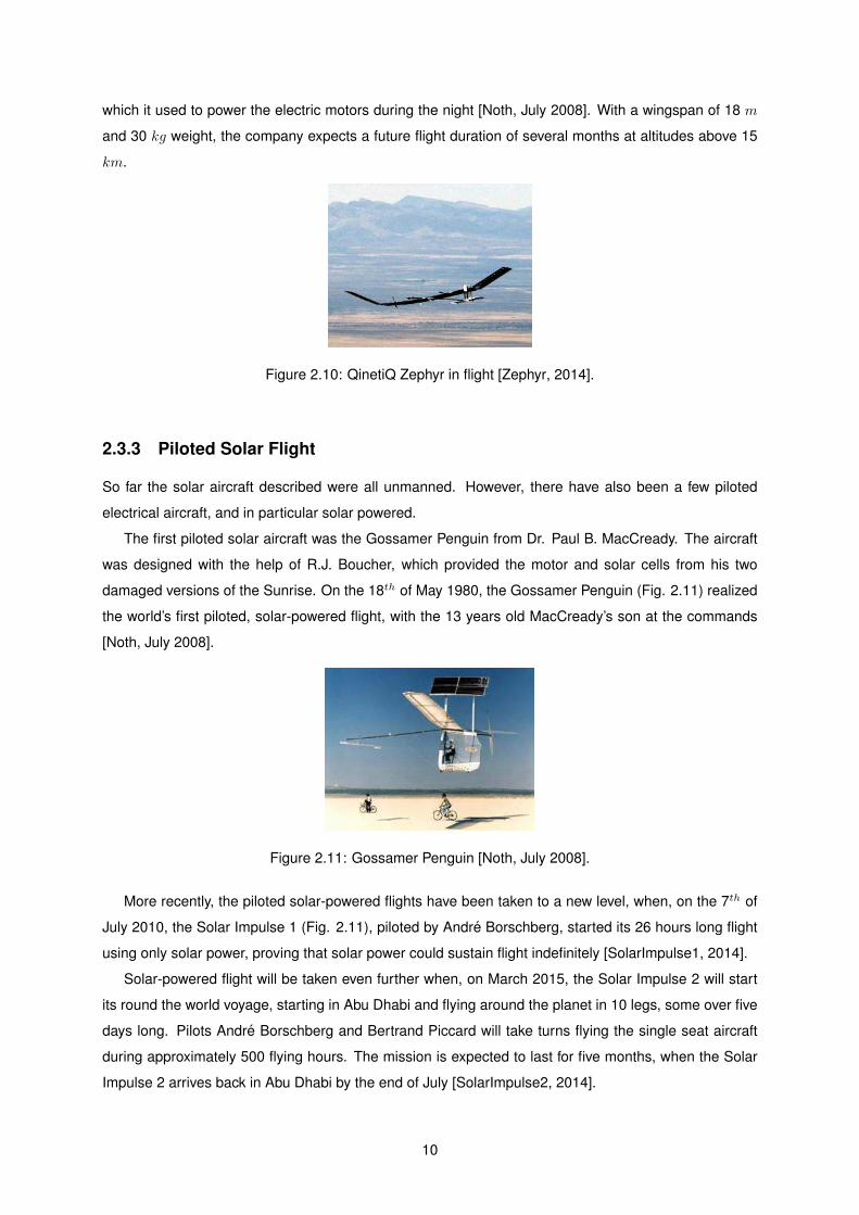
The first approach consisted on designing an aircraft to reach the 30 km altitude objective and another
for the 15 km high long endurance flight, but due to a reduced budget that could only fund one plane, in
early 1999, the Centurion was modified from five wing sections to six wing sections, changing the center
wing section to two new and stronger sections, bringing the wing span up to 75.29 m, while maintaining
the same 14 electric motors, to accomplish the long endurance flight. The upgraded aircraft was called
the Helios (fig. 2.7) [Noll et al., 2004]. The first objective was accomplished on 13th August 2001 reach-
ing a maximum altitude of 29.261 m[Helios, Noth, July 2008]. To accomplish the second goal, the Helios
was fitted with regenerative fuel cell system, consisting of a main regenerative fuel cell on the center
of the aircraft, and two high pressure hydrogen tanks on the center of each wing tip section. Unfortu-
nately, on June 26 of 2003, during a shakedown flight in preparation for a 40 hour long endurance flight,
the aircraft encountered some mild turbulence, which increased the wing dihedral beyond the expected,
causing an oscillating pitch variation, which constantly grew until the wing skin started to separate, caus-
ing the crash of the aircraft in the Pacific ocean. From start to finish, 91 seconds elapsed [Noll et al.,
2004, Helios].
8
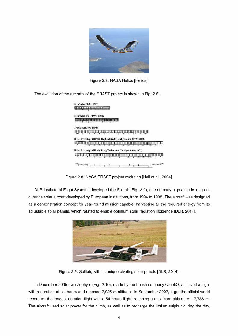
Figure 2.7: NASA Helios [Helios].
The evolution of the aircrafts of the ERAST project is shown in Fig. 2.8.
Figure 2.8: NASA ERAST project evolution [Noll et al., 2004].
DLR Institute of Flight Systems developed the Solitair (Fig. 2.9), one of many high altitude long en-
durance solar aircraft developed by European institutions, from 1994 to 1998. The aircraft was designed
as a demonstration concept for year-round mission capable, harvesting all the required energy from its
adjustable solar panels, which rotated to enable optimum solar radiation incidence [DLR, 2014].
Figure 2.9: Solitair, with its unique pivoting solar panels [DLR, 2014].
In December 2005, two Zephyrs (Fig. 2.10), made by the british company QinetiQ, achieved a flight
with a duration of six hours and reached 7,925 m altitude. In September 2007, it got the official world
record for the longest duration flight with a 54 hours flight, reaching a maximum altitude of 17,786 m.
The aircraft used solar power for the climb, as well as to recharge the lithium-sulphur during the day,
9
which it used to power the electric motors during the night [Noth, July 2008]. With a wingspan of 18 m
and 30 kg weight, the company expects a future flight duration of several months at altitudes above 15
km.
Figure 2.10: QinetiQ Zephyr in flight [Zephyr, 2014].
2.3.3 Piloted Solar Flight
So far the solar aircraft described were all unmanned. However, there have also been a few piloted
electrical aircraft, and in particular solar powered.
The first piloted solar aircraft was the Gossamer Penguin from Dr. Paul B. MacCready. The aircraft
was designed with the help of R.J. Boucher, which provided the motor and solar cells from his two
damaged versions of the Sunrise. On the 18th of May 1980, the Gossamer Penguin (Fig. 2.11) realized
the world’s first piloted, solar-powered flight, with the 13 years old MacCready’s son at the commands
[Noth, July 2008].
Figure 2.11: Gossamer Penguin [Noth, July 2008].
More recently, the piloted solar-powered flights have been taken to a new level, when, on the 7th of
July 2010, the Solar Impulse 1 (Fig. 2.11), piloted by Andre Borschberg, started its 26 hours long flight
using only solar power, proving that solar power could sustain flight indefinitely [SolarImpulse1, 2014].
Solar-powered flight will be taken even further when, on March 2015, the Solar Impulse 2 will start
its round the world voyage, starting in Abu Dhabi and flying around the planet in 10 legs, some over five
days long. Pilots Andre Borschberg and Bertrand Piccard will take turns flying the single seat aircraft
during approximately 500 flying hours. The mission is expected to last for five months, when the Solar
Impulse 2 arrives back in Abu Dhabi by the end of July [SolarImpulse2, 2014].
10
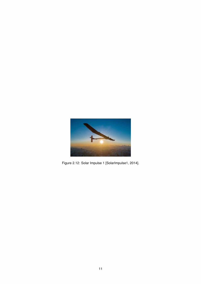
Figure 2.12: Solar Impulse 1 [SolarImpulse1, 2014].
11

12
Chapter 3
Aircraft, Mission and Hybrid
Propulsion
In this chapter, the aircraft characteristics, mission and solutions found will be discussed. This is an
important chapter since these characteristics and decisions will determine the system developed and
tested along the rest of the thesis.
The aircraft is part of a joint project by several research institutes of LAETA [LAETA, 2014], in partic-
ular IDMEC [IDMEC, 2014], CCTAE [CCTAE, 2014],AEROG [AEROG, 2014] and INEGI [INEGI, 2014].
The project kick-started in 2011 and has since had the contribution of several researchers and, most
important, students doing their master dissertation, as is the present case. The previous work, briefly
summarized in this chapter, can be found in more detail in [Marta and Gamboa, 2014].
3.1 Mission
The aircraft has to be tailored for the mission it has to accomplish. So in this section the mission
requirements will be discussed.
The aircraft will be a Long Endurance Electric Unmanned Aerial Vehicle (LEEUAV) for use in civilian
surveillance missions. The objective if to be an affordable platform, with off-the-shelf components, that
can be easily deployed in locations with relative small space, while being able to carry a payload of up
to 1 kg. As for the long endurance, it has to be able to gather, or generate, energy in mid flight to be
able to stay airborne for long durations of time, since the weight of the energy accumulators required for
long duration flights would increase the take-off weight of the vehicle and reduced its payload carrying
capabilities. To demonstrate the viability of the aircraft a mission was proposed:
1. Take-off at ground level, in a very short distance, in an 8 m run on a track or in 3 m if hand
launched;
2. Climb to 1,000m above ground level, for a cruise altitude, in 10 minutes;
3. Flight at a cruise speed of no less than 7 m/s, for 8 hours at equinox;
4. Descend from cruise altitude to ground level without power, in 29 minutes;
13
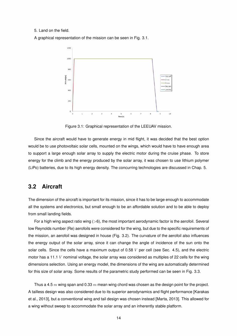
5. Land on the field.
A graphical representation of the mission can be seen in Fig. 3.1.
Figure 3.1: Graphical representation of the LEEUAV mission.
Since the aircraft would have to generate energy in mid flight, it was decided that the best option
would be to use photovoltaic solar cells, mounted on the wings, which would have to have enough area
to support a large enough solar array to supply the electric motor during the cruise phase. To store
energy for the climb and the energy produced by the solar array, it was chosen to use lithium polymer
(LiPo) batteries, due to its high energy density. The concurring technologies are discussed in Chap. 5.
3.2 Aircraft
The dimension of the aircraft is important for its mission, since it has to be large enough to accommodate
all the systems and electronics, but small enough to be an affordable solution and to be able to deploy
from small landing fields.
For a high wing aspect ratio wing (>6), the most important aerodynamic factor is the aerofoil. Several
low Reynolds number (Re) aerofoils were considered for the wing, but due to the specific requirements of
the mission, an aerofoil was designed in house (Fig. 3.2). The curvature of the aerofoil also influences
the energy output of the solar array, since it can change the angle of incidence of the sun onto the
solar cells. Since the cells have a maximum output of 0.58 V per cell (see Sec. 4.5), and the electric
motor has a 11.1 V nominal voltage, the solar array was considered as multiples of 22 cells for the wing
dimensions selection. Using an energy model, the dimensions of the wing are automatically determined
for this size of solar array. Some results of the parametric study performed can be seen in Fig. 3.3.
Thus a 4.5 m wing span and 0.33 m mean wing chord was chosen as the design point for the project.
A tailless design was also considered due to its superior aerodynamics and flight performance [Karakas
et al., 2013], but a conventional wing and tail design was chosen instead [Marta, 2013]. This allowed for
a wing without sweep to accommodate the solar array and an inherently stable platform.
14
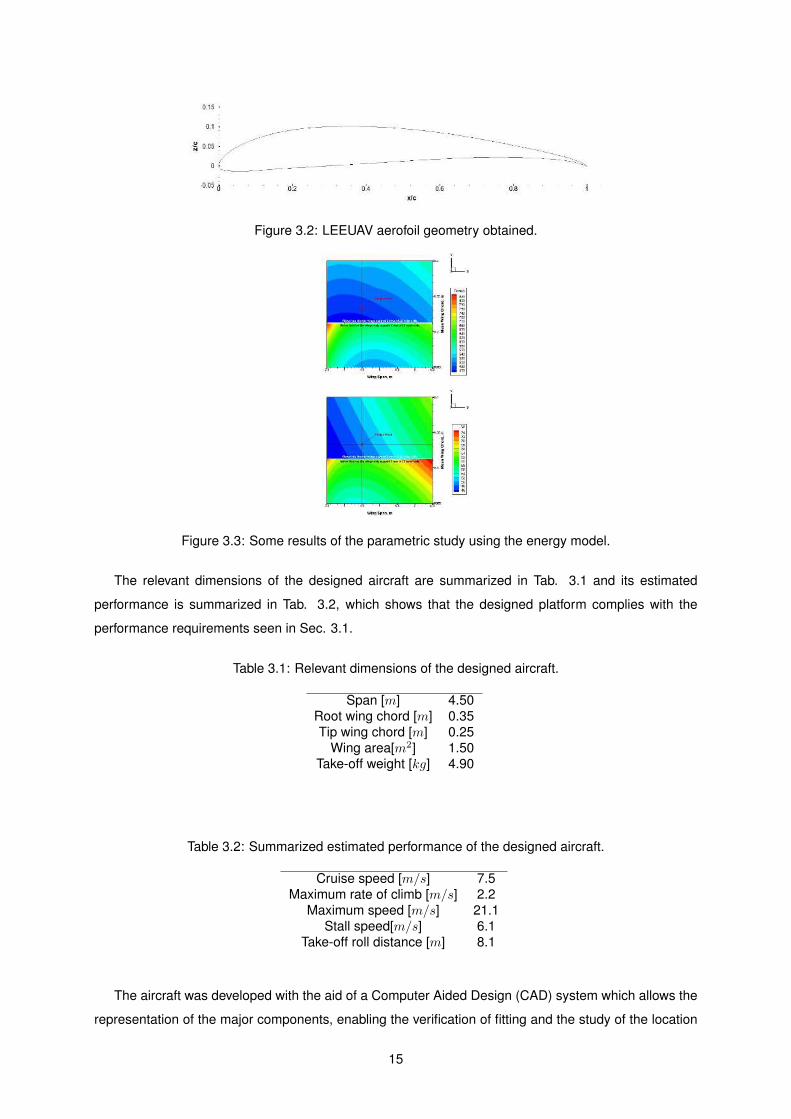
Figure 3.2: LEEUAV aerofoil geometry obtained.
Figure 3.3: Some results of the parametric study using the energy model.
The relevant dimensions of the designed aircraft are summarized in Tab. 3.1 and its estimated
performance is summarized in Tab. 3.2, which shows that the designed platform complies with the
performance requirements seen in Sec. 3.1.
Table 3.1: Relevant dimensions of the designed aircraft.
Span [m] 4.50Root wing chord [m] 0.35Tip wing chord [m] 0.25
Wing area[m2] 1.50Take-off weight [kg] 4.90
Table 3.2: Summarized estimated performance of the designed aircraft.
Cruise speed [m/s] 7.5Maximum rate of climb [m/s] 2.2
Maximum speed [m/s] 21.1Stall speed[m/s] 6.1
Take-off roll distance [m] 8.1
The aircraft was developed with the aid of a Computer Aided Design (CAD) system which allows the
representation of the major components, enabling the verification of fitting and the study of the location
15
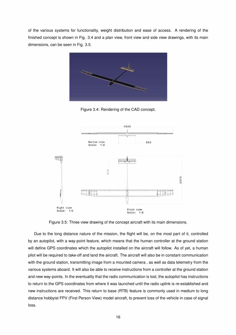
of the various systems for functionality, weight distribution and ease of access. A rendering of the
finished concept is shown in Fig. 3.4 and a plan view, front view and side view drawings, with its main
dimensions, can be seen in Fig. 3.5.
Figure 3.4: Rendering of the CAD concept.
Figure 3.5: Three view drawing of the concept aircraft with its main dimensions.
Due to the long distance nature of the mission, the flight will be, on the most part of it, controlled
by an autopilot, with a way-point feature, which means that the human controller at the ground station
will define GPS coordinates which the autopilot installed on the aircraft will follow. As of yet, a human
pilot will be required to take-off and land the aircraft. The aircraft will also be in constant communication
with the ground station, transmitting image from a mounted camera , as well as data telemetry from the
various systems aboard. It will also be able to receive instructions from a controller at the ground station
and new way-points. In the eventuality that the radio communication is lost, the autopilot has instructions
to return to the GPS coordinates from where it was launched until the radio uplink is re-established and
new instructions are received. This return to base (RTB) feature is commonly used in medium to long
distance hobbyist FPV (First Person View) model aircraft, to prevent loss of the vehicle in case of signal
loss.
16
To allow for the storage and generation of energy required for the successful accomplishment of
the proposed mission, a hybrid propulsion system was designed, using solar panels and an energy
accumulator.
3.3 Hybrid Propulsion
Hybrid means the mixture of two things. In the case of propulsion, it means joining two technologies
to achieve a better way to move. Two driving methods can be combined, like a common hybrid car
with a gasoline engine and an electric engine, both driving the wheels, or two different energy sources
are mixed, like some hybrid cars that have a battery bank but also a fossil fuel generator to charge the
batteries when needed.
In the developed project, a long duration flight of a unmanned aerial vehicle was desired. The
current energy accumulation technologies did not allow the storage of enough energy to sustain the
model airborne over the course of the flight. For this reason, a hybrid propulsion UAV with two energy
sources was designed.
The hybrid system would be accomplished by joining an energy accumulator, which would be charged
prior to the beginning of the flight, and an energy production system. Since this is a model aeroplane,
having a gasoline generator is not an option due to the weight of this system. Therefore an array of solar
cells was deemed the best option, since the wings have a large area, room to put the array was not a
problem.
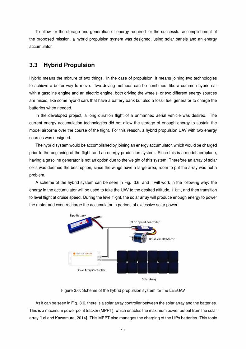
A scheme of the hybrid system can be seen in Fig. 3.6, and it will work in the following way: the
energy in the accumulator will be used to take the UAV to the desired altitude, 1 km, and then transition
to level flight at cruise speed. During the level flight, the solar array will produce enough energy to power
the motor and even recharge the accumulator in periods of excessive solar power.
Figure 3.6: Scheme of the hybrid propulsion system for the LEEUAV
As it can be seen in Fig. 3.6, there is a solar array controller between the solar array and the batteries.
This is a maximum power point tracker (MPPT), which enables the maximum power output from the solar
array [Lei and Kawamura, 2014]. This MPPT also manages the charging of the LiPo batteries. This topic
17

is further discussed in Sec. 4.5.
As for the propulsion part of this system, the UAV will be propelled using the thrust produced by a
out-runner brushless direct current (BLDC) electric motor which will spin a propeller. The BLDC motor
was chosen due to its higher efficiency when compared to common brushed electric motors, although
they require an additional electronic circuit to change the current flow on the coils, changing its magnetic
field, attracting or repelling the magnets on the rotor. In the case of an out runner electric motor, the
permanent magnets are attached to a housing (rotor) which rotates around the stator, which has the
coils. This type of BLDC motors are commonly used to power larger and with higher torque demand
propellers. The number of coils, the number of windings, the number of magnets and the supplied
voltage affect the maximum rotating speed of the motor, as well as the maximum torque.
18
Chapter 4
Solar Cells
4.1 Introduction
A solar cell, or a photovoltaic cell (PV cell), is an electronic equipment that transforms solar radiation
into electricity. It is comprised of two or more semiconductor layers, with different properties, that when
receive light radiation create an electric current. This process is known as the photovoltaic effect.
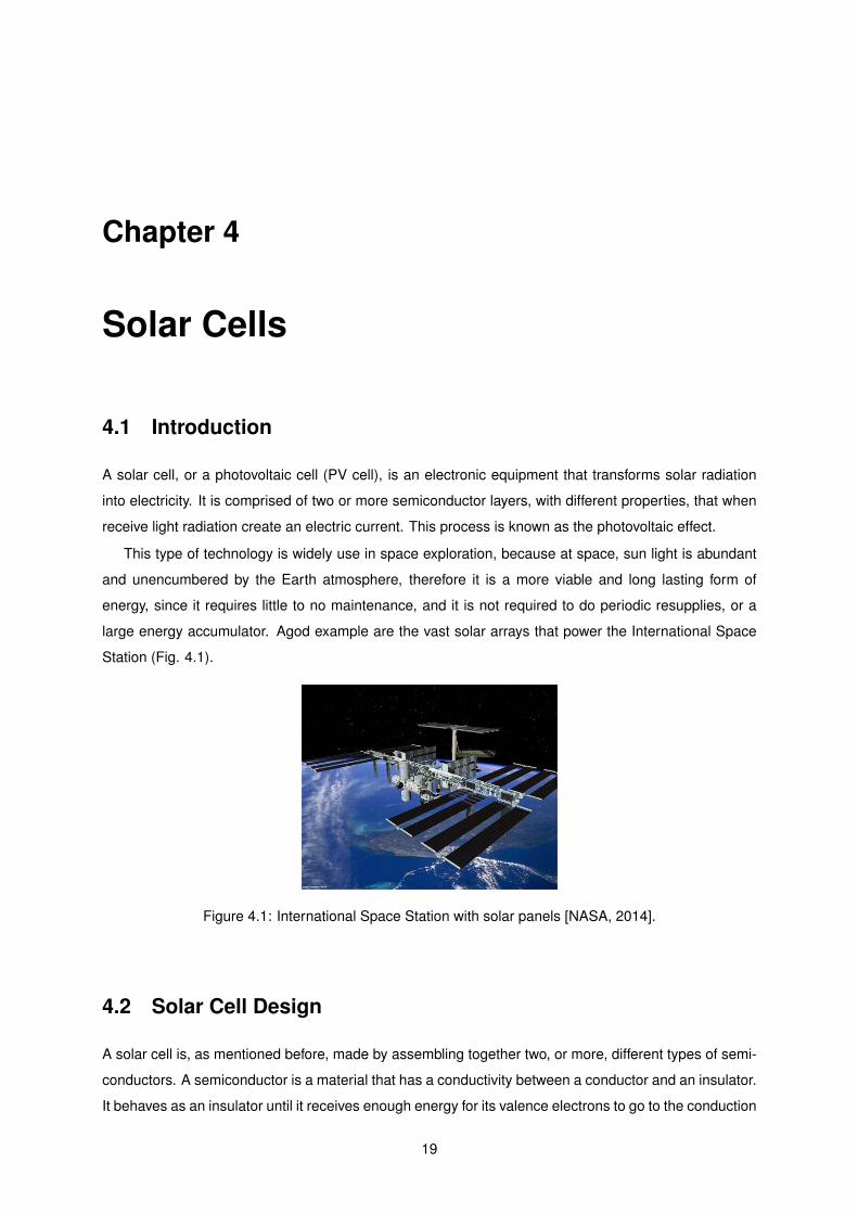
This type of technology is widely use in space exploration, because at space, sun light is abundant
and unencumbered by the Earth atmosphere, therefore it is a more viable and long lasting form of
energy, since it requires little to no maintenance, and it is not required to do periodic resupplies, or a
large energy accumulator. Agod example are the vast solar arrays that power the International Space
Station (Fig. 4.1).
Figure 4.1: International Space Station with solar panels [NASA, 2014].
4.2 Solar Cell Design
A solar cell is, as mentioned before, made by assembling together two, or more, different types of semi-
conductors. A semiconductor is a material that has a conductivity between a conductor and an insulator.
It behaves as an insulator until it receives enough energy for its valence electrons to go to the conduction
19
band. It then behaves like a conductor. The smaller the gap between its valence and conduction bands,
the easier it is to make it conduct electricity. There are 2 main types of semiconductors:
1. i-type: Intrinsic semiconductors are unaltered and pure crystals of semiconductors, i.e. undoped
semiconductors.
2. n-type or p-type: extrinsic semiconductors. This type is altered, doped, to give it different proper-
ties from the pure crystal. This doping is achieved mixing different atoms in the pure crystal.
2.1. n-type semiconductors are treated to have a higher electrons concentration, i.e., they have
electrons that are easier to remove than the pure material.
2.2. p-type are treated to have a deficit of electrons, or holes, so they attract electrons easier.
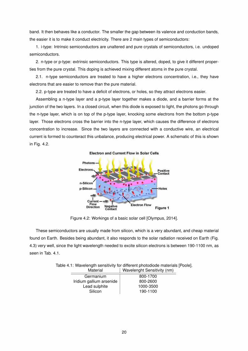
Assembling a n-type layer and a p-type layer together makes a diode, and a barrier forms at the
junction of the two layers. In a closed circuit, when this diode is exposed to light, the photons go through
the n-type layer, which is on top of the p-type layer, knocking some electrons from the bottom p-type
layer. Those electrons cross the barrier into the n-type layer, which causes the difference of electrons
concentration to increase. Since the two layers are connected with a conductive wire, an electrical
current is formed to counteract this unbalance, producing electrical power. A schematic of this is shown
in Fig. 4.2.
Figure 4.2: Workings of a basic solar cell [Olympus, 2014].
These semiconductors are usually made from silicon, which is a very abundant, and cheap material
found on Earth. Besides being abundant, it also responds to the solar radiation received on Earth (Fig.
4.3) very well, since the light wavelength needed to excite silicon electrons is between 190-1100 nm, as
seen in Tab. 4.1.
Table 4.1: Wavelength sensitivity for different photodiode materials [Poole].Material Wavelenght Sensitivity (nm)
Germanium 800-1700Iridium gallium arsenide 800-2600
Lead sulphite 1000-3500Silicon 190-1100
20
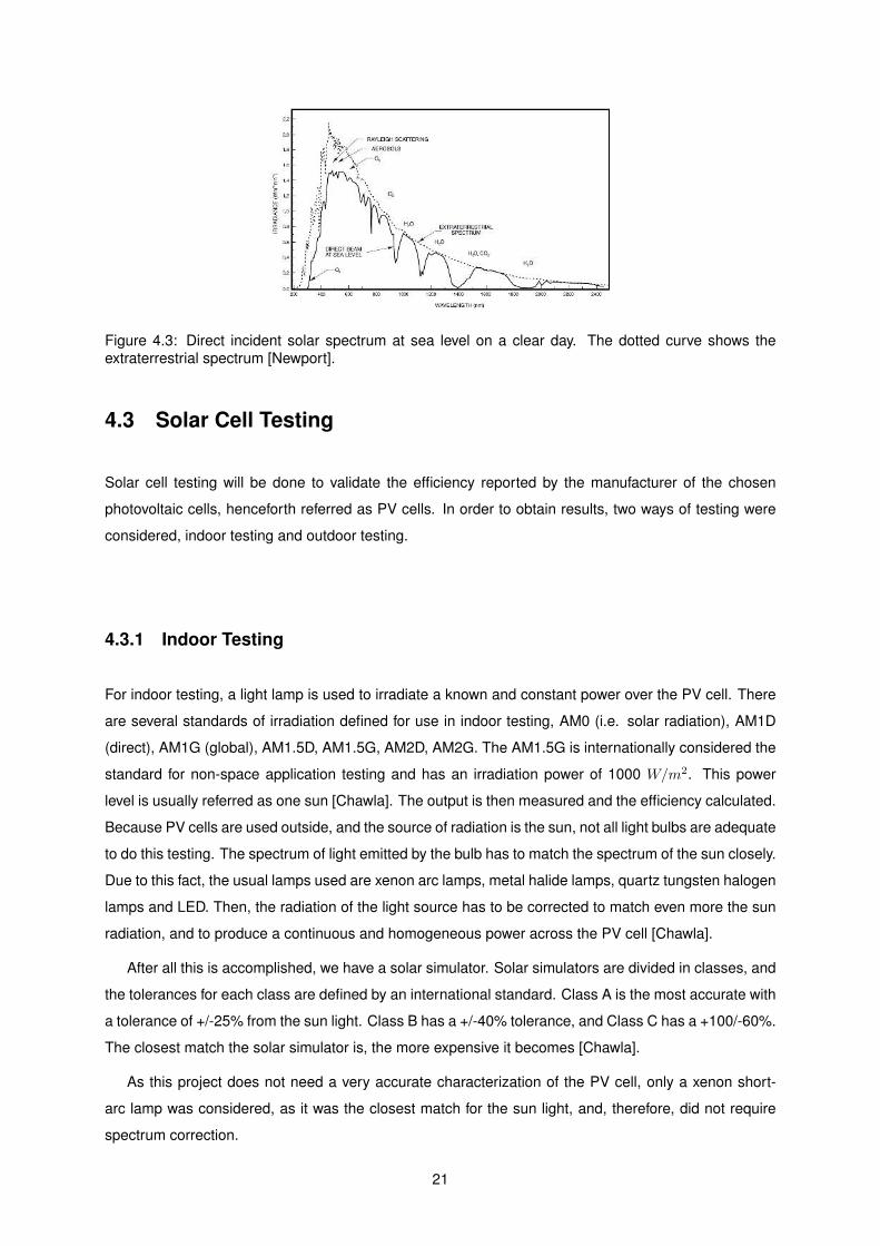
Figure 4.3: Direct incident solar spectrum at sea level on a clear day. The dotted curve shows theextraterrestrial spectrum [Newport].
4.3 Solar Cell Testing
Solar cell testing will be done to validate the efficiency reported by the manufacturer of the chosen
photovoltaic cells, henceforth referred as PV cells. In order to obtain results, two ways of testing were
considered, indoor testing and outdoor testing.
4.3.1 Indoor Testing
For indoor testing, a light lamp is used to irradiate a known and constant power over the PV cell. There
are several standards of irradiation defined for use in indoor testing, AM0 (i.e. solar radiation), AM1D
(direct), AM1G (global), AM1.5D, AM1.5G, AM2D, AM2G. The AM1.5G is internationally considered the
standard for non-space application testing and has an irradiation power of 1000 W/m2. This power
level is usually referred as one sun [Chawla]. The output is then measured and the efficiency calculated.
Because PV cells are used outside, and the source of radiation is the sun, not all light bulbs are adequate
to do this testing. The spectrum of light emitted by the bulb has to match the spectrum of the sun closely.
Due to this fact, the usual lamps used are xenon arc lamps, metal halide lamps, quartz tungsten halogen
lamps and LED. Then, the radiation of the light source has to be corrected to match even more the sun
radiation, and to produce a continuous and homogeneous power across the PV cell [Chawla].
After all this is accomplished, we have a solar simulator. Solar simulators are divided in classes, and
the tolerances for each class are defined by an international standard. Class A is the most accurate with
a tolerance of +/-25% from the sun light. Class B has a +/-40% tolerance, and Class C has a +100/-60%.
The closest match the solar simulator is, the more expensive it becomes [Chawla].
As this project does not need a very accurate characterization of the PV cell, only a xenon short-
arc lamp was considered, as it was the closest match for the sun light, and, therefore, did not require
spectrum correction.
21
4.3.2 Outdoor Testing
For outdoor testing, no artificial light source is necessary because it is possible to use the sun radiation
directly. The problem with this approach is the measure of the input energy on the PV cells. To measure
the sun irradiation, a pyranometer is usually used.
Another method of measuring the irradiation power, is to use a lux meter, and then convert the mea-
sured lux to W/m2. This is not easily accomplished, because lux measures the light power perceived by
the human eye. This means that green or yellow light, at 555 nm wave length, gives a higher lux mea-
sure for the same irradiated power. This means that, either an approximation value is used to convert
lux to W/m2 (usually considered 683lux = 1W/m2 [Photonfocus, 2004]), or an integration of the solar
spectrum with the adjusting coeficient is used. As such, the direct measurement of the solar irradiation
by using a pyranometer is the method of choice.
4.3.3 Testing Method Selection
After consideration of all the approaches, only the outdoor testing was considered. This was due to the
fact that an indoor solar testing device would be too costly and complicated, and since only a approxi-
mate validation of the PV cell is needed, such cost and effort were found to be unnecessary.
Also, for the outdoor testing, it was decided that the best course to take would be to acquire a pyra-
nometer, since the lux meter would also need to be acquired and the approximations are complicated
and, possibly, not be very accurate. There are several pyranometers technologies, with a wide price
range, so some research was done to choose the best option.
4.4 Pyranometer
From the research done on the market, there are three main types of pyranometers available.
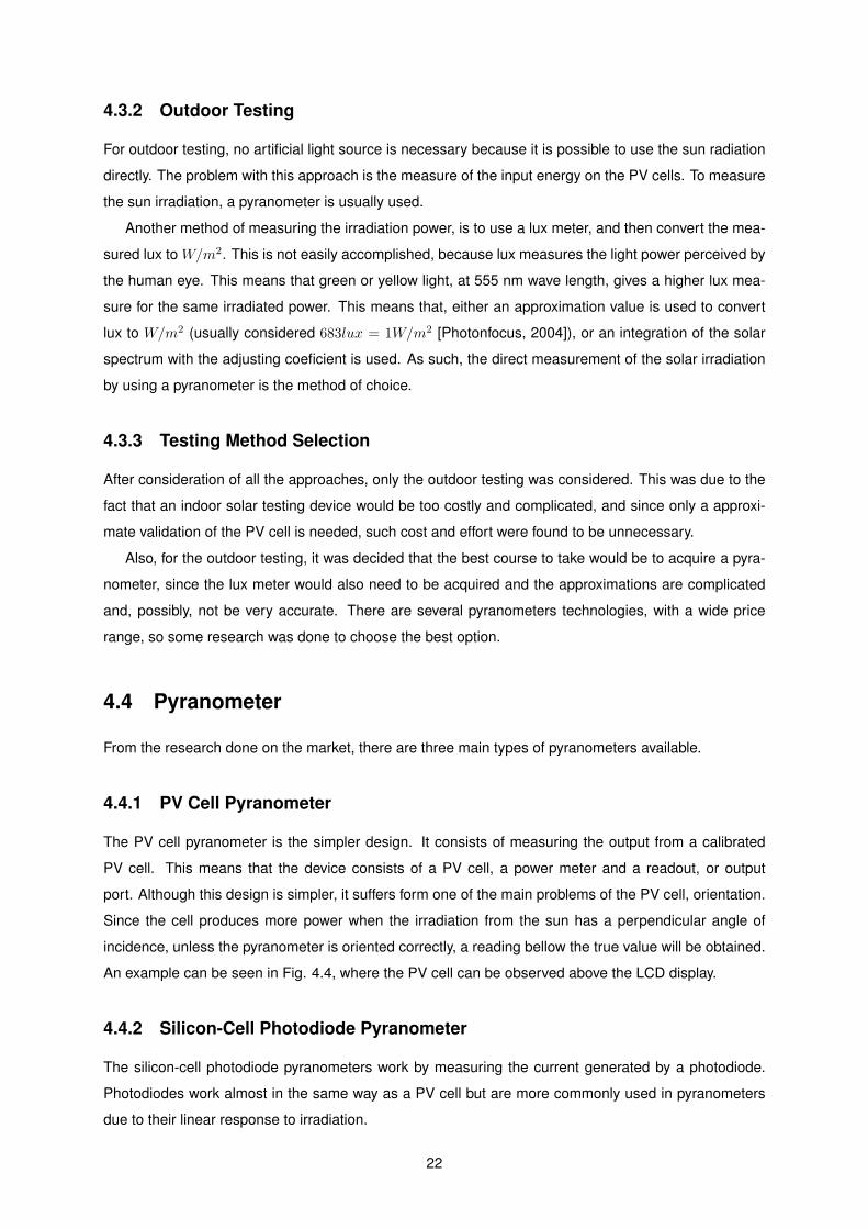
4.4.1 PV Cell Pyranometer
The PV cell pyranometer is the simpler design. It consists of measuring the output from a calibrated
PV cell. This means that the device consists of a PV cell, a power meter and a readout, or output
port. Although this design is simpler, it suffers form one of the main problems of the PV cell, orientation.
Since the cell produces more power when the irradiation from the sun has a perpendicular angle of
incidence, unless the pyranometer is oriented correctly, a reading bellow the true value will be obtained.
An example can be seen in Fig. 4.4, where the PV cell can be observed above the LCD display.
4.4.2 Silicon-Cell Photodiode Pyranometer
The silicon-cell photodiode pyranometers work by measuring the current generated by a photodiode.
Photodiodes work almost in the same way as a PV cell but are more commonly used in pyranometers
due to their linear response to irradiation.
22
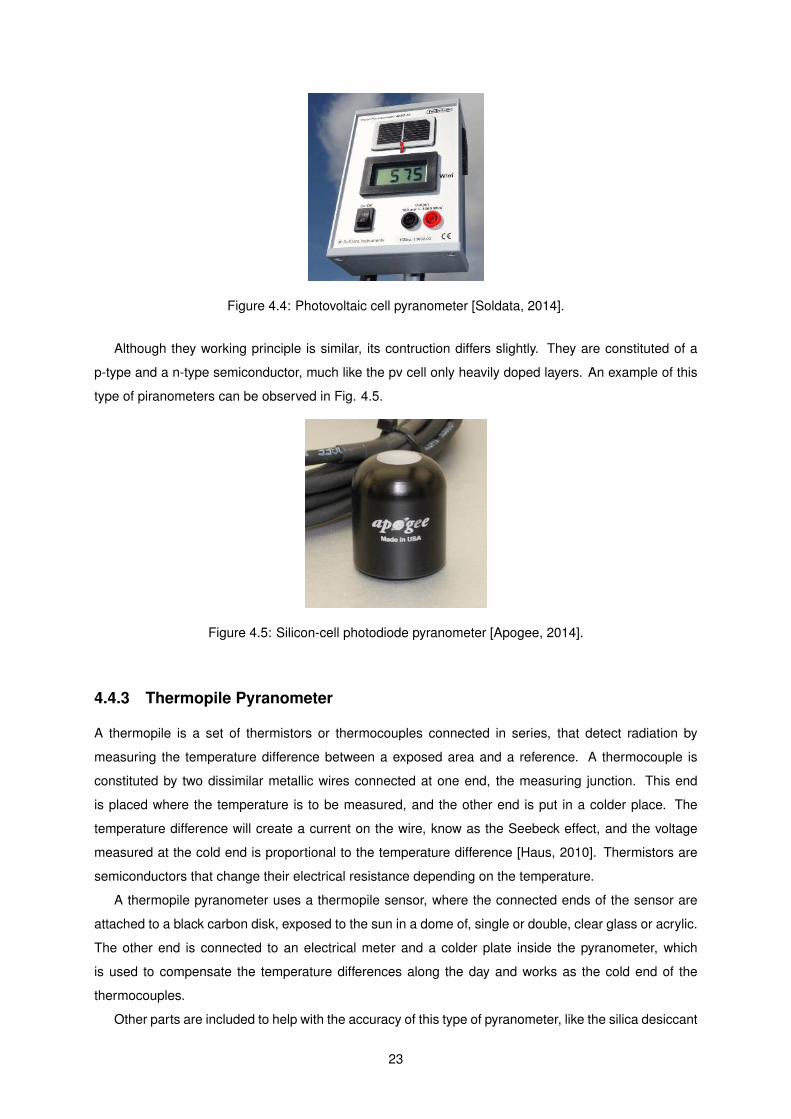
Figure 4.4: Photovoltaic cell pyranometer [Soldata, 2014].
Although they working principle is similar, its contruction differs slightly. They are constituted of a
p-type and a n-type semiconductor, much like the pv cell only heavily doped layers. An example of this
type of piranometers can be observed in Fig. 4.5.
Figure 4.5: Silicon-cell photodiode pyranometer [Apogee, 2014].
4.4.3 Thermopile Pyranometer
A thermopile is a set of thermistors or thermocouples connected in series, that detect radiation by
measuring the temperature difference between a exposed area and a reference. A thermocouple is
constituted by two dissimilar metallic wires connected at one end, the measuring junction. This end
is placed where the temperature is to be measured, and the other end is put in a colder place. The
temperature difference will create a current on the wire, know as the Seebeck effect, and the voltage
measured at the cold end is proportional to the temperature difference [Haus, 2010]. Thermistors are
semiconductors that change their electrical resistance depending on the temperature.
A thermopile pyranometer uses a thermopile sensor, where the connected ends of the sensor are
attached to a black carbon disk, exposed to the sun in a dome of, single or double, clear glass or acrylic.
The other end is connected to an electrical meter and a colder plate inside the pyranometer, which
is used to compensate the temperature differences along the day and works as the cold end of the
thermocouples.
Other parts are included to help with the accuracy of this type of pyranometer, like the silica desiccant
23
to eliminate the dew inside the domes, as well as the design of the outer shell to facilitate the elimination
of dust and rain, as illustrated in Fig. 4.6.
Figure 4.6: Thermopile pyranometer constitution [GlobalSpec, 2014].
An example of this tpe of piranometer can be observed in Fig. 4.7.
Figure 4.7: Thermopile pyranometer [EKO, 2014].
4.5 MPPT
The MPPT (maximum power point tracking) is an electronic device that varies the electrical operating
point of the solar array to extract the maximum power possible.
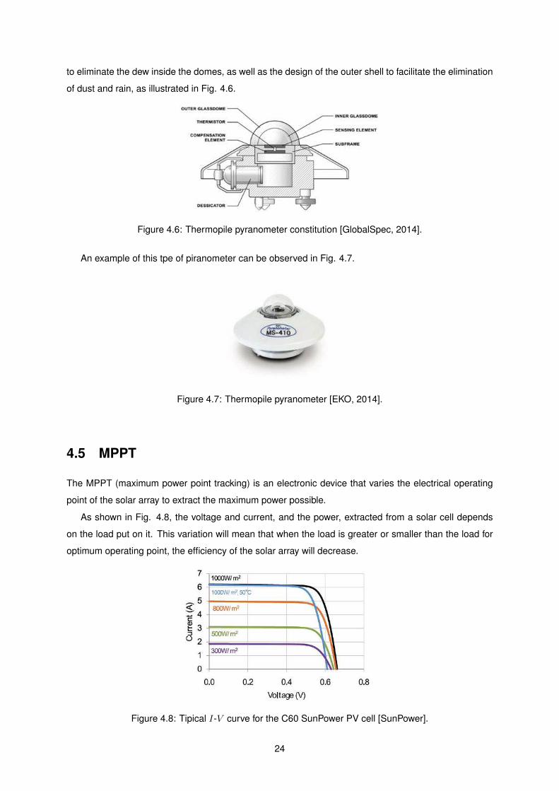
As shown in Fig. 4.8, the voltage and current, and the power, extracted from a solar cell depends
on the load put on it. This variation will mean that when the load is greater or smaller than the load for
optimum operating point, the efficiency of the solar array will decrease.
Figure 4.8: Tipical I-V curve for the C60 SunPower PV cell [SunPower].
24

To counteract this effect, a MPPT module is placed between the solar array and the load, in many
cases a charging battery, thus guaranteeing that the solar array is always outputting its maximum power
and efficiency. In the case of the curve shown in Fig. 4.8, the maximum power output for a PV cell at
25oC would have a voltage of 0,58 V .
25

26
Chapter 5
Energy Accumulator
It is possible to accumulate energy using various methods, but not all are usable in this project. This
chapter will address some types of energy accumulators.
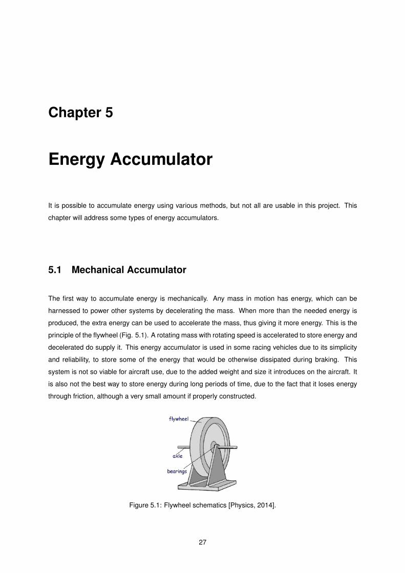
5.1 Mechanical Accumulator
The first way to accumulate energy is mechanically. Any mass in motion has energy, which can be
harnessed to power other systems by decelerating the mass. When more than the needed energy is
produced, the extra energy can be used to accelerate the mass, thus giving it more energy. This is the
principle of the flywheel (Fig. 5.1). A rotating mass with rotating speed is accelerated to store energy and
decelerated do supply it. This energy accumulator is used in some racing vehicles due to its simplicity
and reliability, to store some of the energy that would be otherwise dissipated during braking. This
system is not so viable for aircraft use, due to the added weight and size it introduces on the aircraft. It
is also not the best way to store energy during long periods of time, due to the fact that it loses energy
through friction, although a very small amount if properly constructed.
Figure 5.1: Flywheel schematics [Physics, 2014].
27
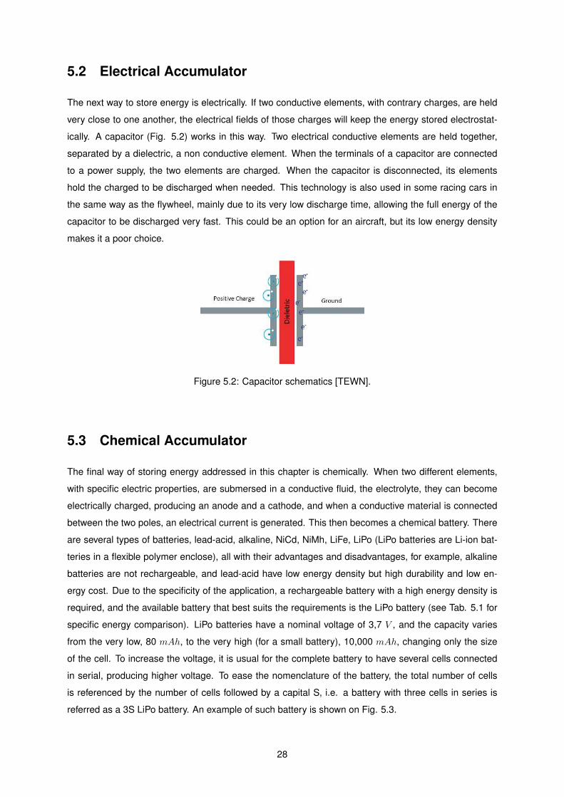
5.2 Electrical Accumulator
The next way to store energy is electrically. If two conductive elements, with contrary charges, are held
very close to one another, the electrical fields of those charges will keep the energy stored electrostat-
ically. A capacitor (Fig. 5.2) works in this way. Two electrical conductive elements are held together,
separated by a dielectric, a non conductive element. When the terminals of a capacitor are connected
to a power supply, the two elements are charged. When the capacitor is disconnected, its elements
hold the charged to be discharged when needed. This technology is also used in some racing cars in
the same way as the flywheel, mainly due to its very low discharge time, allowing the full energy of the
capacitor to be discharged very fast. This could be an option for an aircraft, but its low energy density
makes it a poor choice.
Figure 5.2: Capacitor schematics [TEWN].
5.3 Chemical Accumulator
The final way of storing energy addressed in this chapter is chemically. When two different elements,
with specific electric properties, are submersed in a conductive fluid, the electrolyte, they can become
electrically charged, producing an anode and a cathode, and when a conductive material is connected
between the two poles, an electrical current is generated. This then becomes a chemical battery. There
are several types of batteries, lead-acid, alkaline, NiCd, NiMh, LiFe, LiPo (LiPo batteries are Li-ion bat-
teries in a flexible polymer enclose), all with their advantages and disadvantages, for example, alkaline
batteries are not rechargeable, and lead-acid have low energy density but high durability and low en-
ergy cost. Due to the specificity of the application, a rechargeable battery with a high energy density is
required, and the available battery that best suits the requirements is the LiPo battery (see Tab. 5.1 for
specific energy comparison). LiPo batteries have a nominal voltage of 3,7 V , and the capacity varies
from the very low, 80 mAh, to the very high (for a small battery), 10,000 mAh, changing only the size
of the cell. To increase the voltage, it is usual for the complete battery to have several cells connected
in serial, producing higher voltage. To ease the nomenclature of the battery, the total number of cells
is referenced by the number of cells followed by a capital S, i.e. a battery with three cells in series is
referred as a 3S LiPo battery. An example of such battery is shown on Fig. 5.3.
28
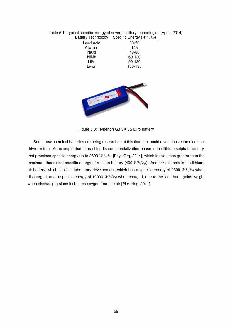
Table 5.1: Typical specific energy of several battery technologies [Epec, 2014].Battery Technology Specific Energy (Wh/kg)
Lead Acid 30-50Alkaline 145
NiCd 48-80NiMh 60-120LiFe 90-120Li-ion 100-190
Figure 5.3: Hyperion G3 VX 3S LiPo battery
Some new chemical batteries are being researched at this time that could revolutionize the electrical
drive system. An example that is reaching its commercialization phase is the lithium-sulphate battery,
that promises specific energy up to 2600 Wh/kg [Phys.Org, 2014], which is five times greater than the
maximum theoretical specific energy of a Li-ion battery (400 Wh/kg). Another example is the lithium-
air battery, which is still in laboratory development, which has a specific energy of 2600 Wh/kg when
discharged, and a specific energy of 10000 Wh/kg when charged, due to the fact that it gains weight
when discharging since it absorbs oxygen from the air [Pickering, 2011].
29

30
Chapter 6
Sensors and Data Acquisition System
To fully characterize the hybrid propulsion system, some sensors will have to be used to measure the
parameters required. In this system, there will be electrical components as well as force and thermal
generating components. For this reason, some different sensors will be needed to measure all the
parameters of the system.
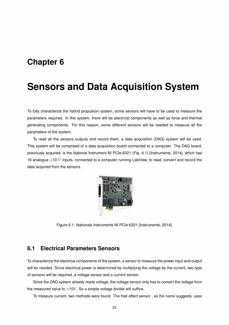
To read all the sensors outputs and record them, a data acquisition (DAQ) system will be used.
This system will be comprised of a data acquisition board connected to a computer. The DAQ board,
previously acquired, is the National Instrument NI PCIe-6321 (Fig. 6.1) [Instruments, 2014], which has
16 analogue ±10 V inputs, connected to a computer running LabView, to read, convert and record the
data acquired from the sensors.
Figure 6.1: Nationals Instruments NI PCIe-6321 [Instruments, 2014].
6.1 Electrical Parameters Sensors
To characterize the electrical components of the system, a sensor to measure the power input and output
will be needed. Since electrical power is determined by multiplying the voltage by the current, two type
of sensors will be required, a voltage sensor and a current sensor.
Since the DAQ system already reads voltage, the voltage sensor only has to convert the voltage from
the measured value to ±10V . So a simple voltage divider will suffice.
To measure current, two methods were found. The Hall effect sensor , as the name suggests, uses
31
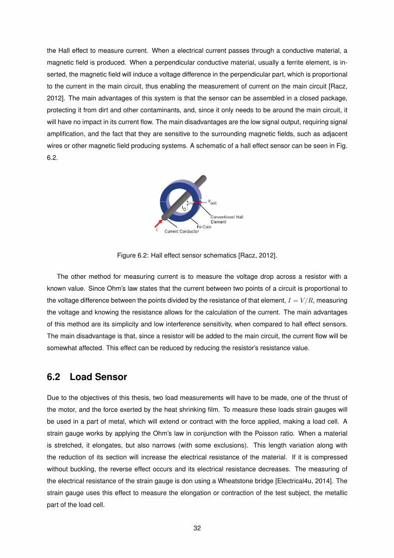
the Hall effect to measure current. When a electrical current passes through a conductive material, a
magnetic field is produced. When a perpendicular conductive material, usually a ferrite element, is in-
serted, the magnetic field will induce a voltage difference in the perpendicular part, which is proportional
to the current in the main circuit, thus enabling the measurement of current on the main circuit [Racz,
2012]. The main advantages of this system is that the sensor can be assembled in a closed package,
protecting it from dirt and other contaminants, and, since it only needs to be around the main circuit, it
will have no impact in its current flow. The main disadvantages are the low signal output, requiring signal
amplification, and the fact that they are sensitive to the surrounding magnetic fields, such as adjacent
wires or other magnetic field producing systems. A schematic of a hall effect sensor can be seen in Fig.
6.2.
Figure 6.2: Hall effect sensor schematics [Racz, 2012].
The other method for measuring current is to measure the voltage drop across a resistor with a
known value. Since Ohm’s law states that the current between two points of a circuit is proportional to
the voltage difference between the points divided by the resistance of that element, I = V/R, measuring
the voltage and knowing the resistance allows for the calculation of the current. The main advantages
of this method are its simplicity and low interference sensitivity, when compared to hall effect sensors.
The main disadvantage is that, since a resistor will be added to the main circuit, the current flow will be
somewhat affected. This effect can be reduced by reducing the resistor’s resistance value.
6.2 Load Sensor
Due to the objectives of this thesis, two load measurements will have to be made, one of the thrust of
the motor, and the force exerted by the heat shrinking film. To measure these loads strain gauges will
be used in a part of metal, which will extend or contract with the force applied, making a load cell. A
strain gauge works by applying the Ohm’s law in conjunction with the Poisson ratio. When a material
is stretched, it elongates, but also narrows (with some exclusions). This length variation along with
the reduction of its section will increase the electrical resistance of the material. If it is compressed
without buckling, the reverse effect occurs and its electrical resistance decreases. The measuring of
the electrical resistance of the strain gauge is don using a Wheatstone bridge [Electrical4u, 2014]. The
strain gauge uses this effect to measure the elongation or contraction of the test subject, the metallic
part of the load cell.
32
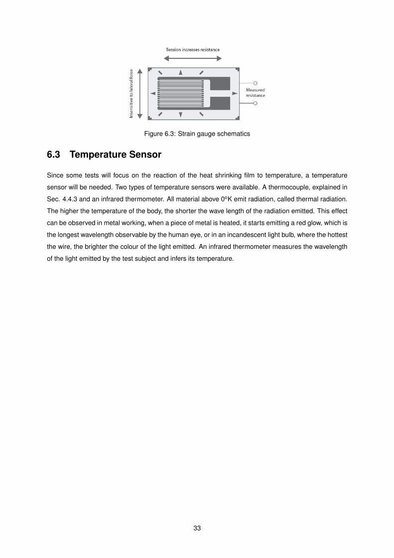
Figure 6.3: Strain gauge schematics
6.3 Temperature Sensor
Since some tests will focus on the reaction of the heat shrinking film to temperature, a temperature
sensor will be needed. Two types of temperature sensors were available. A thermocouple, explained in
Sec. 4.4.3 and an infrared thermometer. All material above 0oK emit radiation, called thermal radiation.
The higher the temperature of the body, the shorter the wave length of the radiation emitted. This effect
can be observed in metal working, when a piece of metal is heated, it starts emitting a red glow, which is
the longest wavelength observable by the human eye, or in an incandescent light bulb, where the hottest
the wire, the brighter the colour of the light emitted. An infrared thermometer measures the wavelength
of the light emitted by the test subject and infers its temperature.
33

34
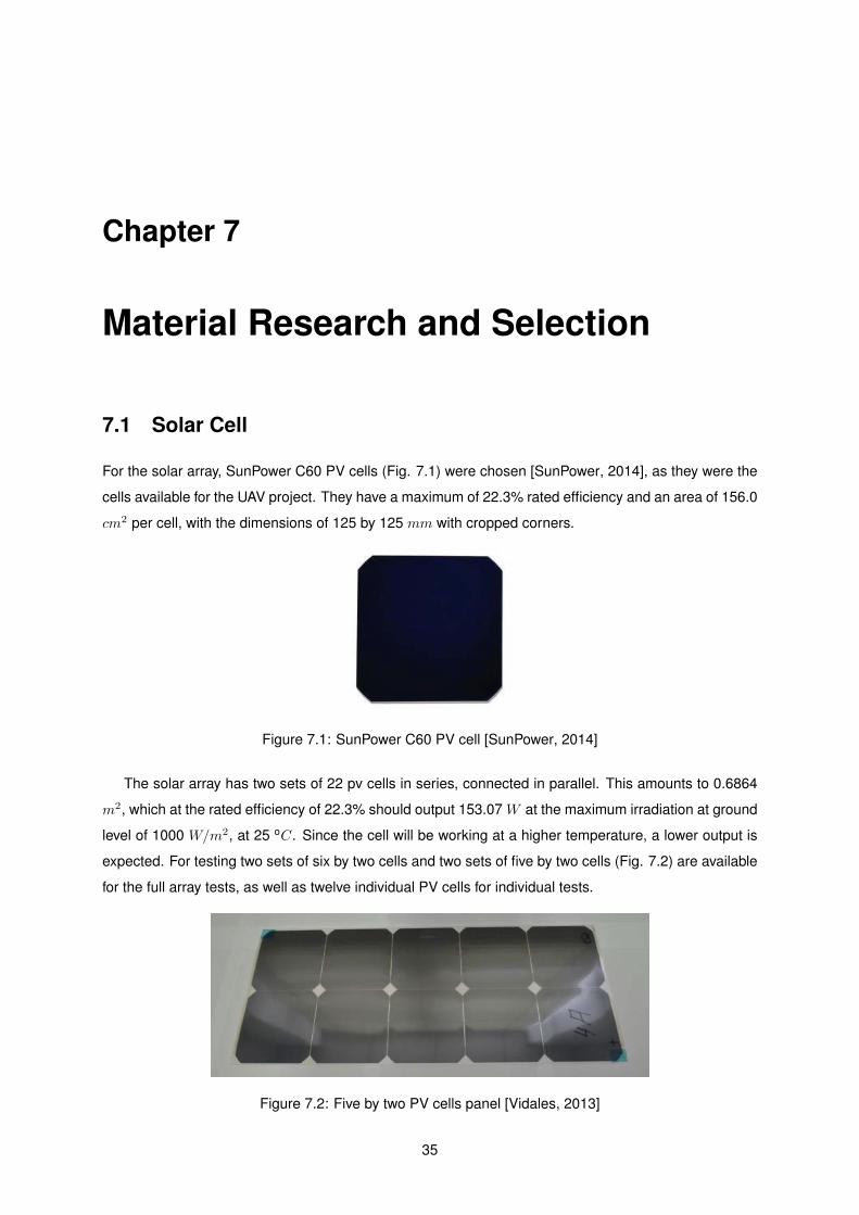
Chapter 7
Material Research and Selection
7.1 Solar Cell
For the solar array, SunPower C60 PV cells (Fig. 7.1) were chosen [SunPower, 2014], as they were the
cells available for the UAV project. They have a maximum of 22.3% rated efficiency and an area of 156.0
cm2 per cell, with the dimensions of 125 by 125 mm with cropped corners.
Figure 7.1: SunPower C60 PV cell [SunPower, 2014]
The solar array has two sets of 22 pv cells in series, connected in parallel. This amounts to 0.6864
m2, which at the rated efficiency of 22.3% should output 153.07 W at the maximum irradiation at ground
level of 1000 W/m2, at 25 oC. Since the cell will be working at a higher temperature, a lower output is
expected. For testing two sets of six by two cells and two sets of five by two cells (Fig. 7.2) are available
for the full array tests, as well as twelve individual PV cells for individual tests.
Figure 7.2: Five by two PV cells panel [Vidales, 2013]
35
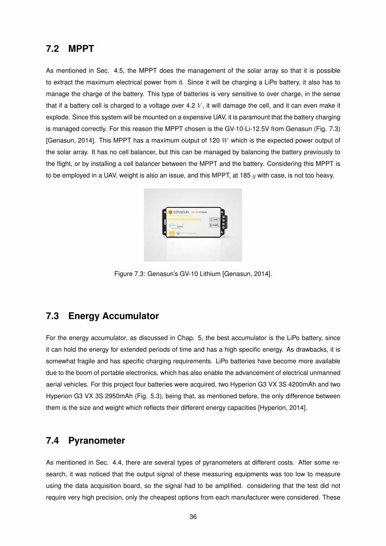
7.2 MPPT
As mentioned in Sec. 4.5, the MPPT does the management of the solar array so that it is possible
to extract the maximum electrical power from it. Since it will be charging a LiPo battery, it also has to
manage the charge of the battery. This type of batteries is very sensitive to over charge, in the sense
that if a battery cell is charged to a voltage over 4.2 V , it will damage the cell, and it can even make it
explode. Since this system will be mounted on a expensive UAV, it is paramount that the battery charging
is managed correctly. For this reason the MPPT chosen is the GV-10-Li-12.5V from Genasun (Fig. 7.3)
[Genasun, 2014]. This MPPT has a maximum output of 120 W which is the expected power output of
the solar array. It has no cell balancer, but this can be managed by balancing the battery previously to
the flight, or by installing a cell balancer between the MPPT and the battery. Considering this MPPT is
to be employed in a UAV, weight is also an issue, and this MPPT, at 185 g with case, is not too heavy.
Figure 7.3: Genasun’s GV-10 Lithium [Genasun, 2014].
7.3 Energy Accumulator
For the energy accumulator, as discussed in Chap. 5, the best accumulator is the LiPo battery, since
it can hold the energy for extended periods of time and has a high specific energy. As drawbacks, it is
somewhat fragile and has specific charging requirements. LiPo batteries have become more available
due to the boom of portable electronics, which has also enable the advancement of electrical unmanned
aerial vehicles. For this project four batteries were acquired, two Hyperion G3 VX 3S 4200mAh and two
Hyperion G3 VX 3S 2950mAh (Fig. 5.3), being that, as mentioned before, the only difference between
them is the size and weight which reflects their different energy capacities [Hyperion, 2014].
7.4 Pyranometer
As mentioned in Sec. 4.4, there are several types of pyranometers at different costs. After some re-
search, it was noticed that the output signal of these measuring equipments was too low to measure
using the data acquisition board, so the signal had to be amplified. considering that the test did not
require very high precision, only the cheapest options from each manufacturer were considered. These
36
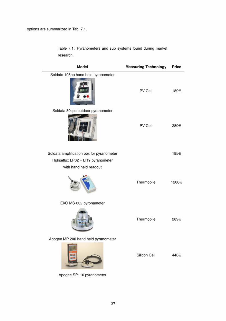
options are summarized in Tab. 7.1.
Table 7.1: Pyranometers and sub systems found during market
research.
Model Measuring Technology Price
Soldata 105hp hand held pyranometer
PV Cell 189e
Soldata 80spc outdoor pyranometer
PV Cell 289e
Soldata amplification box for pyranometer 185e
Hukseflux LP02 + LI19 pyranometer
with hand held readout
Thermopile 1200e
EKO MS-602 pyronameter
Thermopile 289e
Apogee MP 200 hand held pyranometer
Silicon Cell 448e
Apogee SP110 pyranometer
37
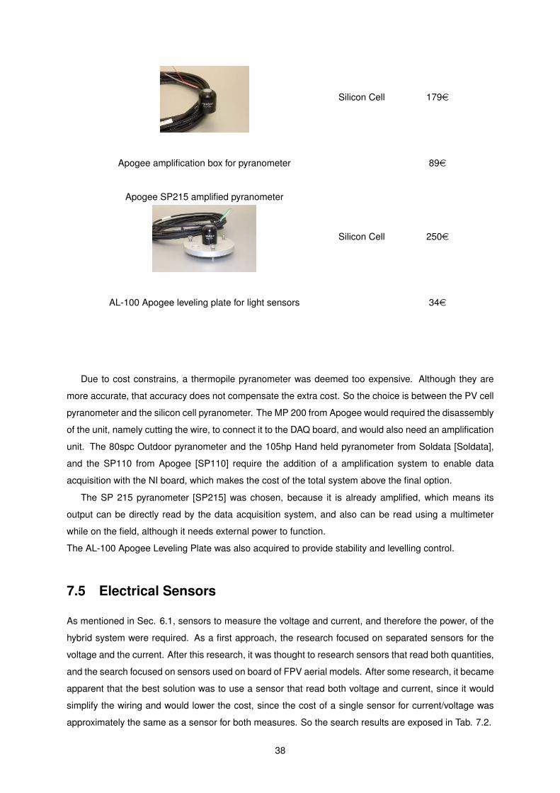
Silicon Cell 179e
Apogee amplification box for pyranometer 89e
Apogee SP215 amplified pyranometer
Silicon Cell 250e
AL-100 Apogee leveling plate for light sensors 34e
Due to cost constrains, a thermopile pyranometer was deemed too expensive. Although they are
more accurate, that accuracy does not compensate the extra cost. So the choice is between the PV cell
pyranometer and the silicon cell pyranometer. The MP 200 from Apogee would required the disassembly
of the unit, namely cutting the wire, to connect it to the DAQ board, and would also need an amplification
unit. The 80spc Outdoor pyranometer and the 105hp Hand held pyranometer from Soldata [Soldata],
and the SP110 from Apogee [SP110] require the addition of a amplification system to enable data
acquisition with the NI board, which makes the cost of the total system above the final option.
The SP 215 pyranometer [SP215] was chosen, because it is already amplified, which means its
output can be directly read by the data acquisition system, and also can be read using a multimeter
while on the field, although it needs external power to function.
The AL-100 Apogee Leveling Plate was also acquired to provide stability and levelling control.
7.5 Electrical Sensors
As mentioned in Sec. 6.1, sensors to measure the voltage and current, and therefore the power, of the
hybrid system were required. As a first approach, the research focused on separated sensors for the
voltage and the current. After this research, it was thought to research sensors that read both quantities,
and the search focused on sensors used on board of FPV aerial models. After some research, it became
apparent that the best solution was to use a sensor that read both voltage and current, since it would
simplify the wiring and would lower the cost, since the cost of a single sensor for current/voltage was
approximately the same as a sensor for both measures. So the search results are exposed in Tab. 7.2.
38
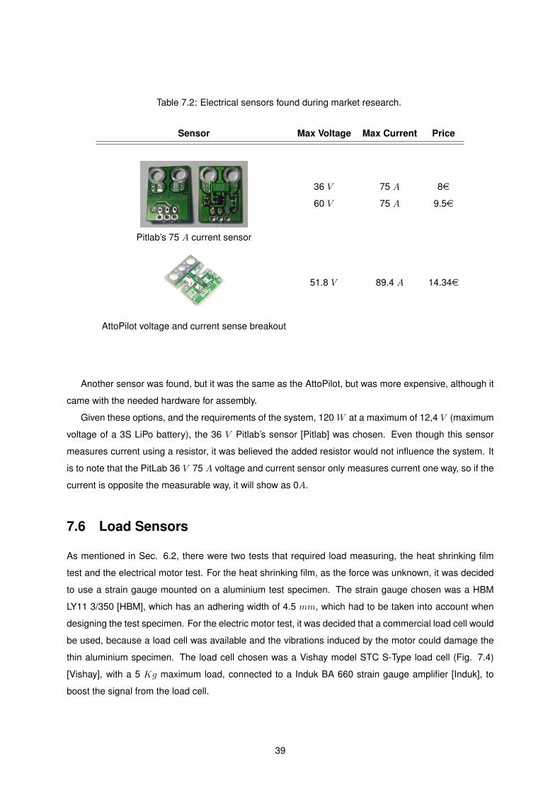
Table 7.2: Electrical sensors found during market research.
Sensor Max Voltage Max Current Price
36 V 75 A 8e
60 V 75 A 9.5e
Pitlab’s 75 A current sensor
51.8 V 89.4 A 14.34e
AttoPilot voltage and current sense breakout
Another sensor was found, but it was the same as the AttoPilot, but was more expensive, although it
came with the needed hardware for assembly.
Given these options, and the requirements of the system, 120 W at a maximum of 12,4 V (maximum
voltage of a 3S LiPo battery), the 36 V Pitlab’s sensor [Pitlab] was chosen. Even though this sensor
measures current using a resistor, it was believed the added resistor would not influence the system. It
is to note that the PitLab 36 V 75 A voltage and current sensor only measures current one way, so if the
current is opposite the measurable way, it will show as 0A.
7.6 Load Sensors
As mentioned in Sec. 6.2, there were two tests that required load measuring, the heat shrinking film
test and the electrical motor test. For the heat shrinking film, as the force was unknown, it was decided
to use a strain gauge mounted on a aluminium test specimen. The strain gauge chosen was a HBM
LY11 3/350 [HBM], which has an adhering width of 4.5 mm, which had to be taken into account when
designing the test specimen. For the electric motor test, it was decided that a commercial load cell would
be used, because a load cell was available and the vibrations induced by the motor could damage the
thin aluminium specimen. The load cell chosen was a Vishay model STC S-Type load cell (Fig. 7.4)
[Vishay], with a 5 Kg maximum load, connected to a Induk BA 660 strain gauge amplifier [Induk], to
boost the signal from the load cell.
39
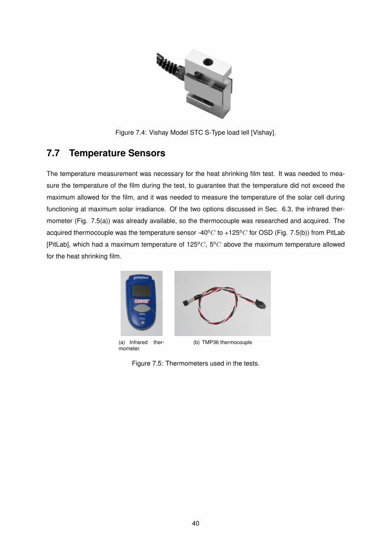
Figure 7.4: Vishay Model STC S-Type load lell [Vishay].
7.7 Temperature Sensors
The temperature measurement was necessary for the heat shrinking film test. It was needed to mea-
sure the temperature of the film during the test, to guarantee that the temperature did not exceed the
maximum allowed for the film, and it was needed to measure the temperature of the solar cell during
functioning at maximum solar irradiance. Of the two options discussed in Sec. 6.3, the infrared ther-
mometer (Fig. 7.5(a)) was already available, so the thermocouple was researched and acquired. The
acquired thermocouple was the temperature sensor -40oC to +125oC for OSD (Fig. 7.5(b)) from PitLab
[PitLab], which had a maximum temperature of 125oC, 5oC above the maximum temperature allowed
for the heat shrinking film.
(a) Infrared ther-mometer.
(b) TMP36 thermocouple
Figure 7.5: Thermometers used in the tests.
40

Chapter 8
Sub Systems Testing
8.1 Electrical Sensor Calibration
Due to the fact that some discrepancies can occur during the manufacture of the sensor, and to under-
stand how accurate it can be, all the used sensors were calibrated when possible.
Both PitLab 36 V 75 A electrical sensors were calibrated using an available professional grade
multimeter. To calibrate these sensors, two test were executed. The first, aimed to calibrate the voltage
sensor, was done by connecting both the sensor and the multimeter to a variable power supply, that
could go from 12 V up to 30 V . Then the voltage was increased by 1 V , from 12 V to 30 V , and
the readings from the multimeter and sensor were recorded. The readings from the sensor had some
interference, so the reading was done by collecting 20 samples at 20 Hz and running it through a filter
that averaged those 20 samples, displaying that average in a numeric readout, as well as in a chart,
and recording it in a file. For the calculations, four averages were used. Screenshots of the developed
LabView program are displayed on Fig. 8.1.
As shown in Fig. 8.0(a), the program enabled to manually enter, the value read in the multimeter, so
that the readings from the sensor and the multimeter were written together in the same data file. To limit
the size of the data file, a record button was added to allow the control of only writing the pertinent data.
After obtaining the data, it was plotted and a linear regression was used to obtain the calibration formula
for the sensor. The result can be seen in Fig. 8.1.
The current calibration was done using 12 V 21 W automotive light bulbs. Considering high power
rated resistors are difficult to acquire as well as expensive, this was considered the best option, enabling
low and high currents by changing the electrical system connected to the power supply. The data
acquisition program was the same as the previous test, as the program was made with both tests in
mind. The data treatment was also done similarly to the voltage calibration. The result is shown on Fig.
8.2.
The information from the manufacturer stated that these sensors had a voltage divider of 16:1 and
a voltage to current conversion of 15.39 A measured (AM ) per V output (VO). As can be seen in the
previous results, Fig. 8.1, for this sensor the conversion factor for the voltage was 15.737 measured
41
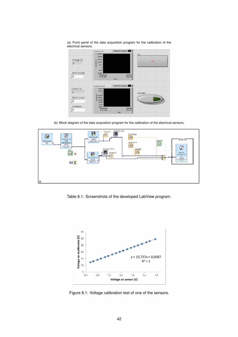
(a) Front panel of the data acquisition program for the calibration of theelectrical sensors.
(b) Block diagram of the data acquisition program for the calibration of the electrical sensors.
Table 8.1: Screenshots of the developed LabView program.
Figure 8.1: Voltage calibration test of one of the sensors.
42
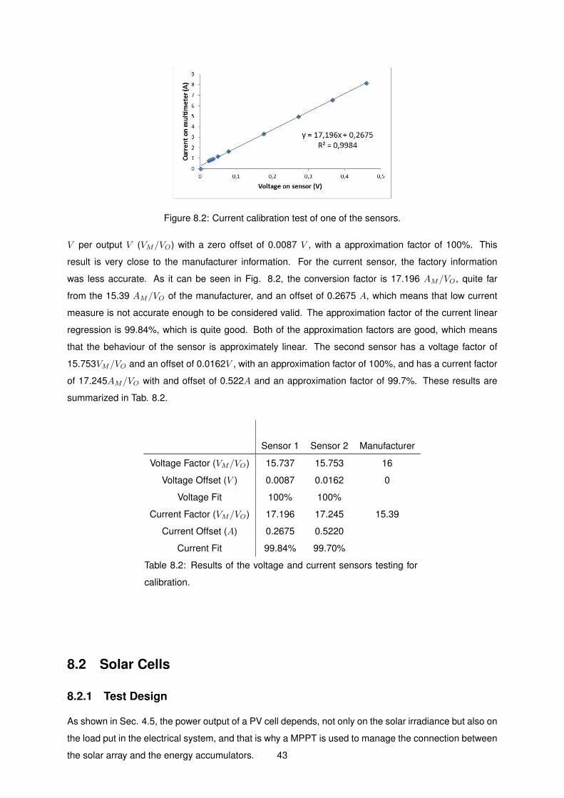
Figure 8.2: Current calibration test of one of the sensors.
V per output V (VM/VO) with a zero offset of 0.0087 V , with a approximation factor of 100%. This
result is very close to the manufacturer information. For the current sensor, the factory information
was less accurate. As it can be seen in Fig. 8.2, the conversion factor is 17.196 AM/VO, quite far
from the 15.39 AM/VO of the manufacturer, and an offset of 0.2675 A, which means that low current
measure is not accurate enough to be considered valid. The approximation factor of the current linear
regression is 99.84%, which is quite good. Both of the approximation factors are good, which means
that the behaviour of the sensor is approximately linear. The second sensor has a voltage factor of
15.753VM/VO and an offset of 0.0162V , with an approximation factor of 100%, and has a current factor
of 17.245AM/VO with and offset of 0.522A and an approximation factor of 99.7%. These results are
summarized in Tab. 8.2.
Sensor 1 Sensor 2 Manufacturer
Voltage Factor (VM/VO) 15.737 15.753 16
Voltage Offset (V ) 0.0087 0.0162 0
Voltage Fit 100% 100%
Current Factor (VM/VO) 17.196 17.245 15.39
Current Offset (A) 0.2675 0.5220
Current Fit 99.84% 99.70%
Table 8.2: Results of the voltage and current sensors testing for
calibration.
8.2 Solar Cells
8.2.1 Test Design
As shown in Sec. 4.5, the power output of a PV cell depends, not only on the solar irradiance but also on
the load put in the electrical system, and that is why a MPPT is used to manage the connection between
the solar array and the energy accumulators. 43
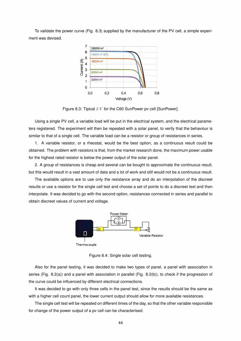
To validate the power curve (Fig. 8.3) supplied by the manufacturer of the PV cell, a simple experi-
ment was devised.
Figure 8.3: Tipical I-V for the C60 SunPower pv cell [SunPower].
Using a single PV cell, a variable load will be put in the electrical system, and the electrical parame-
ters registered. The experiment will then be repeated with a solar panel, to verify that the behaviour is
similar to that of a single cell. The variable load can be a resistor or group of resistances in series.
1. A variable resistor, or a rheostat, would be the best option, as a continuous result could be
obtained. The problem with resistors is that, from the market research done, the maximum power usable
for the highest rated resistor is below the power output of the solar panel.
2. A group of resistances is cheap and several can be bought to approximate the continuous result,
but this would result in a vast amount of data and a lot of work and still would not be a continuous result.
The available options are to use only the resistance array and do an interpolation of the discreet
results or use a resistor for the single cell test and choose a set of points to do a discreet test and then
interpolate. It was decided to go with the second option, resistances connected in series and parallel to
obtain discreet values of current and voltage.
Figure 8.4: Single solar cell testing.
Also for the panel testing, it was decided to make two types of panel, a panel with association in
series (Fig. 8.2(a)) and a panel with association in parallel (Fig. 8.2(b)), to check if the progression of
the curve could be influenced by different electrical connections.
It was decided to go with only three cells in the panel test, since the results should be the same as
with a higher cell count panel, the lower current output should allow for more available resistances.
The single cell test will be repeated on different times of the day, so that the other variable responsible
for change of the power output of a pv cell can be characterised.
44
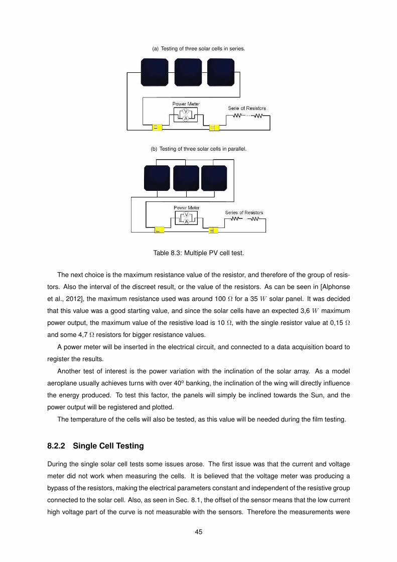
(a) Testing of three solar cells in series.
(b) Testing of three solar cells in parallel.
Table 8.3: Multiple PV cell test.
The next choice is the maximum resistance value of the resistor, and therefore of the group of resis-
tors. Also the interval of the discreet result, or the value of the resistors. As can be seen in [Alphonse
et al., 2012], the maximum resistance used was around 100 Ω for a 35 W solar panel. It was decided
that this value was a good starting value, and since the solar cells have an expected 3,6 W maximum
power output, the maximum value of the resistive load is 10 Ω, with the single resistor value at 0,15 Ω
and some 4,7 Ω resistors for bigger resistance values.
A power meter will be inserted in the electrical circuit, and connected to a data acquisition board to
register the results.
Another test of interest is the power variation with the inclination of the solar array. As a model
aeroplane usually achieves turns with over 40o banking, the inclination of the wing will directly influence
the energy produced. To test this factor, the panels will simply be inclined towards the Sun, and the
power output will be registered and plotted.
The temperature of the cells will also be tested, as this value will be needed during the film testing.
8.2.2 Single Cell Testing
During the single solar cell tests some issues arose. The first issue was that the current and voltage
meter did not work when measuring the cells. It is believed that the voltage meter was producing a
bypass of the resistors, making the electrical parameters constant and independent of the resistive group
connected to the solar cell. Also, as seen in Sec. 8.1, the offset of the sensor means that the low current
high voltage part of the curve is not measurable with the sensors. Therefore the measurements were
45
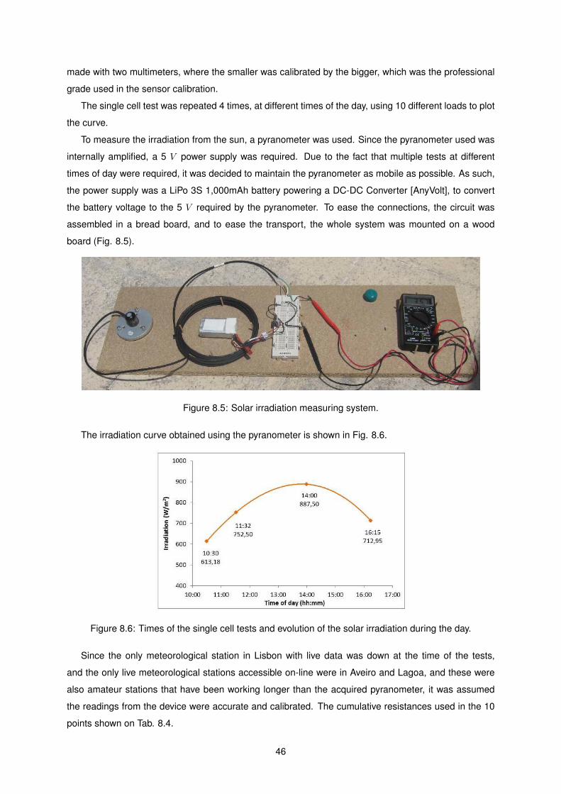
made with two multimeters, where the smaller was calibrated by the bigger, which was the professional
grade used in the sensor calibration.
The single cell test was repeated 4 times, at different times of the day, using 10 different loads to plot
the curve.
To measure the irradiation from the sun, a pyranometer was used. Since the pyranometer used was
internally amplified, a 5 V power supply was required. Due to the fact that multiple tests at different
times of day were required, it was decided to maintain the pyranometer as mobile as possible. As such,
the power supply was a LiPo 3S 1,000mAh battery powering a DC-DC Converter [AnyVolt], to convert
the battery voltage to the 5 V required by the pyranometer. To ease the connections, the circuit was
assembled in a bread board, and to ease the transport, the whole system was mounted on a wood
board (Fig. 8.5).
Figure 8.5: Solar irradiation measuring system.
The irradiation curve obtained using the pyranometer is shown in Fig. 8.6.
Figure 8.6: Times of the single cell tests and evolution of the solar irradiation during the day.
Since the only meteorological station in Lisbon with live data was down at the time of the tests,
and the only live meteorological stations accessible on-line were in Aveiro and Lagoa, and these were
also amateur stations that have been working longer than the acquired pyranometer, it was assumed
the readings from the device were accurate and calibrated. The cumulative resistances used in the 10
points shown on Tab. 8.4.
46
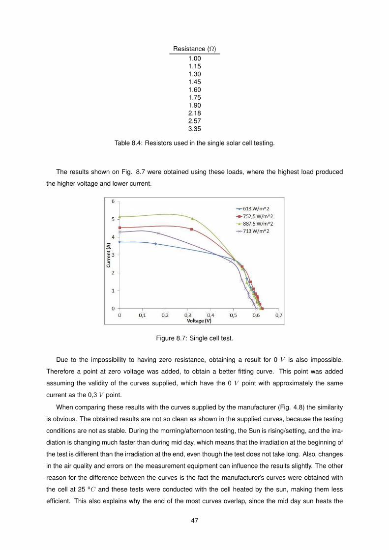
Resistance (Ω)
1.001.151.301.451.601.751.902.182.573.35
Table 8.4: Resistors used in the single solar cell testing.
The results shown on Fig. 8.7 were obtained using these loads, where the highest load produced
the higher voltage and lower current.
Figure 8.7: Single cell test.
Due to the impossibility to having zero resistance, obtaining a result for 0 V is also impossible.
Therefore a point at zero voltage was added, to obtain a better fitting curve. This point was added
assuming the validity of the curves supplied, which have the 0 V point with approximately the same
current as the 0,3 V point.
When comparing these results with the curves supplied by the manufacturer (Fig. 4.8) the similarity
is obvious. The obtained results are not so clean as shown in the supplied curves, because the testing
conditions are not as stable. During the morning/afternoon testing, the Sun is rising/setting, and the irra-
diation is changing much faster than during mid day, which means that the irradiation at the beginning of
the test is different than the irradiation at the end, even though the test does not take long. Also, changes
in the air quality and errors on the measurement equipment can influence the results slightly. The other
reason for the difference between the curves is the fact the manufacturer’s curves were obtained with
the cell at 25 oC and these tests were conducted with the cell heated by the sun, making them less
efficient. This also explains why the end of the most curves overlap, since the mid day sun heats the
47
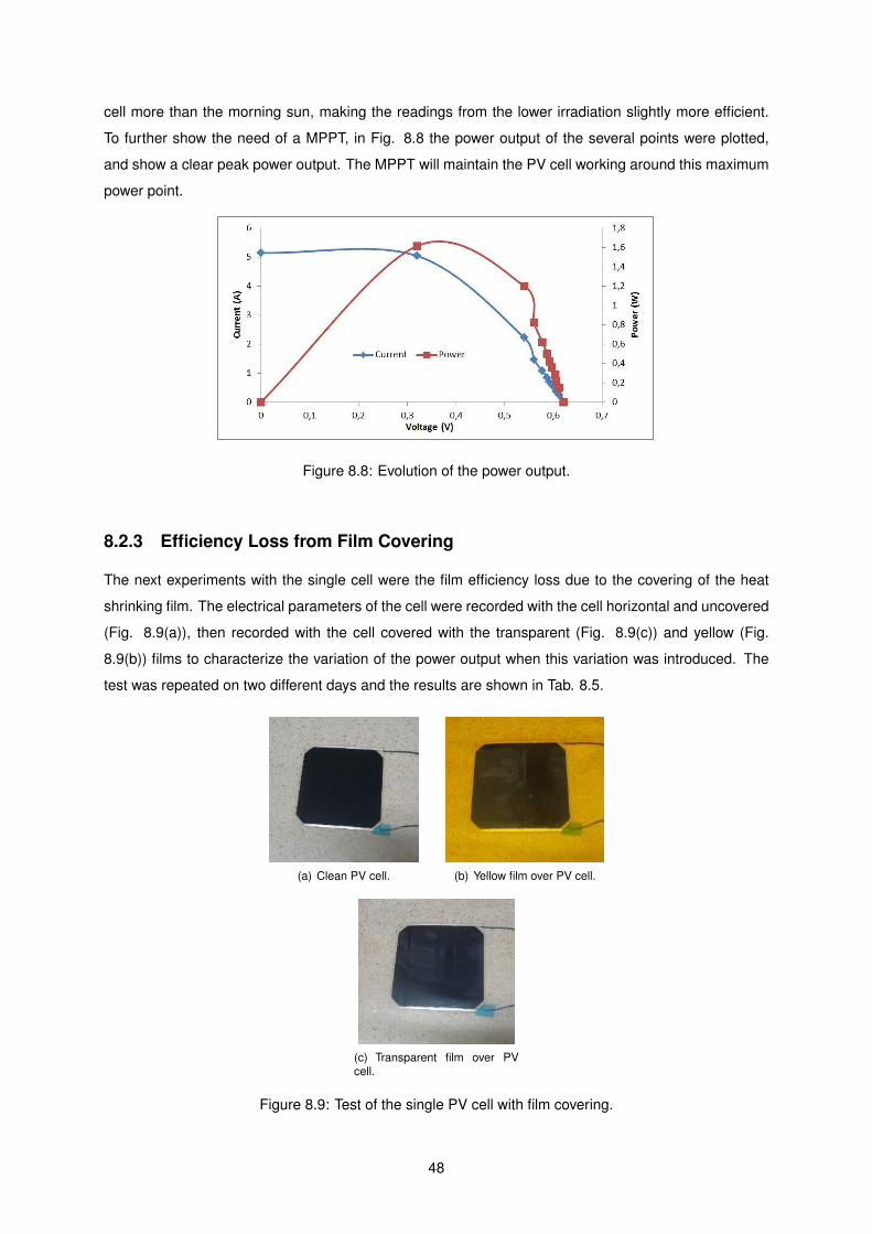
cell more than the morning sun, making the readings from the lower irradiation slightly more efficient.
To further show the need of a MPPT, in Fig. 8.8 the power output of the several points were plotted,
and show a clear peak power output. The MPPT will maintain the PV cell working around this maximum
power point.
Figure 8.8: Evolution of the power output.
8.2.3 Efficiency Loss from Film Covering
The next experiments with the single cell were the film efficiency loss due to the covering of the heat
shrinking film. The electrical parameters of the cell were recorded with the cell horizontal and uncovered
(Fig. 8.9(a)), then recorded with the cell covered with the transparent (Fig. 8.9(c)) and yellow (Fig.
8.9(b)) films to characterize the variation of the power output when this variation was introduced. The
test was repeated on two different days and the results are shown in Tab. 8.5.
(a) Clean PV cell. (b) Yellow film over PV cell.
(c) Transparent film over PVcell.
Figure 8.9: Test of the single PV cell with film covering.
48
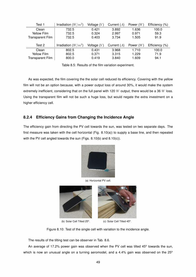
Test 1 Irradiation (W/m2) Voltage (V ) Current (A) Power (W ) Efficiency (%)
Clean 732.5 0.421 3.892 1.636 100.0Yellow Film 732.5 0.324 2.997 0.971 59.3
Transparent Film 732.5 0.403 3.734 1.505 91.9
Test 2 Irradiation (W/m2) Voltage (V ) Current (A) Power (W ) Efficiency (%)
Clean 802.5 0.431 3.968 1.710 100.0Yellow Film 802.5 0.371 3.315 1.229 71.9
Transparent Film 800.0 0.419 3.840 1.609 94.1
Table 8.5: Results of the film variation experiment.
As was expected, the film covering the the solar cell reduced its efficiency. Covering with the yellow
film will not be an option because, with a power output loss of around 30%, it would make the system
extremely inefficient, considering that on the full panel with 120 W output, there would be a 36 W loss.
Using the transparent film will not be such a huge loss, but would negate the extra investment on a
higher efficiency cell.
8.2.4 Efficiency Gains from Changing the Incidence Angle
The efficiency gain from directing the PV cell towards the sun, was tested on two separate days. The
first measure was taken with the cell horizontal (Fig. 8.10(a)) to supply a base line, and then repeated
with the PV cell angled towards the sun (Figs. 8.10(b) and 8.10(c)).
(a) Horizontal PV cell.
(b) Solar Cell Tilted 25o. (c) Solar Cell Tilted 45o.
Figure 8.10: Test of the single cell with variation to the incidence angle.
The results of the tilting test can be observer in Tab. 8.6.
An average of 17.2% power gain was observed when the PV cell was tilted 45o towards the sun,
which is now an unusual angle on a turning aeromodel, and a 4.4% gain was observed on the 25o
49
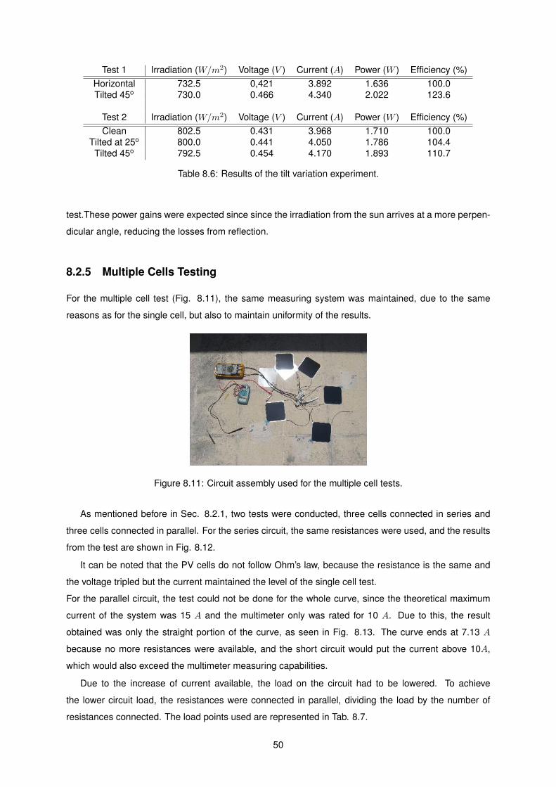
Test 1 Irradiation (W/m2) Voltage (V ) Current (A) Power (W ) Efficiency (%)
Horizontal 732.5 0,421 3.892 1.636 100.0Tilted 45o 730.0 0.466 4.340 2.022 123.6
Test 2 Irradiation (W/m2) Voltage (V ) Current (A) Power (W ) Efficiency (%)
Clean 802.5 0.431 3.968 1.710 100.0Tilted at 25o 800.0 0.441 4.050 1.786 104.4
Tilted 45o 792.5 0.454 4.170 1.893 110.7
Table 8.6: Results of the tilt variation experiment.
test.These power gains were expected since since the irradiation from the sun arrives at a more perpen-
dicular angle, reducing the losses from reflection.
8.2.5 Multiple Cells Testing
For the multiple cell test (Fig. 8.11), the same measuring system was maintained, due to the same
reasons as for the single cell, but also to maintain uniformity of the results.
Figure 8.11: Circuit assembly used for the multiple cell tests.
As mentioned before in Sec. 8.2.1, two tests were conducted, three cells connected in series and
three cells connected in parallel. For the series circuit, the same resistances were used, and the results
from the test are shown in Fig. 8.12.
It can be noted that the PV cells do not follow Ohm’s law, because the resistance is the same and
the voltage tripled but the current maintained the level of the single cell test.
For the parallel circuit, the test could not be done for the whole curve, since the theoretical maximum
current of the system was 15 A and the multimeter only was rated for 10 A. Due to this, the result
obtained was only the straight portion of the curve, as seen in Fig. 8.13. The curve ends at 7.13 A
because no more resistances were available, and the short circuit would put the current above 10A,
which would also exceed the multimeter measuring capabilities.
Due to the increase of current available, the load on the circuit had to be lowered. To achieve
the lower circuit load, the resistances were connected in parallel, dividing the load by the number of
resistances connected. The load points used are represented in Tab. 8.7.
50
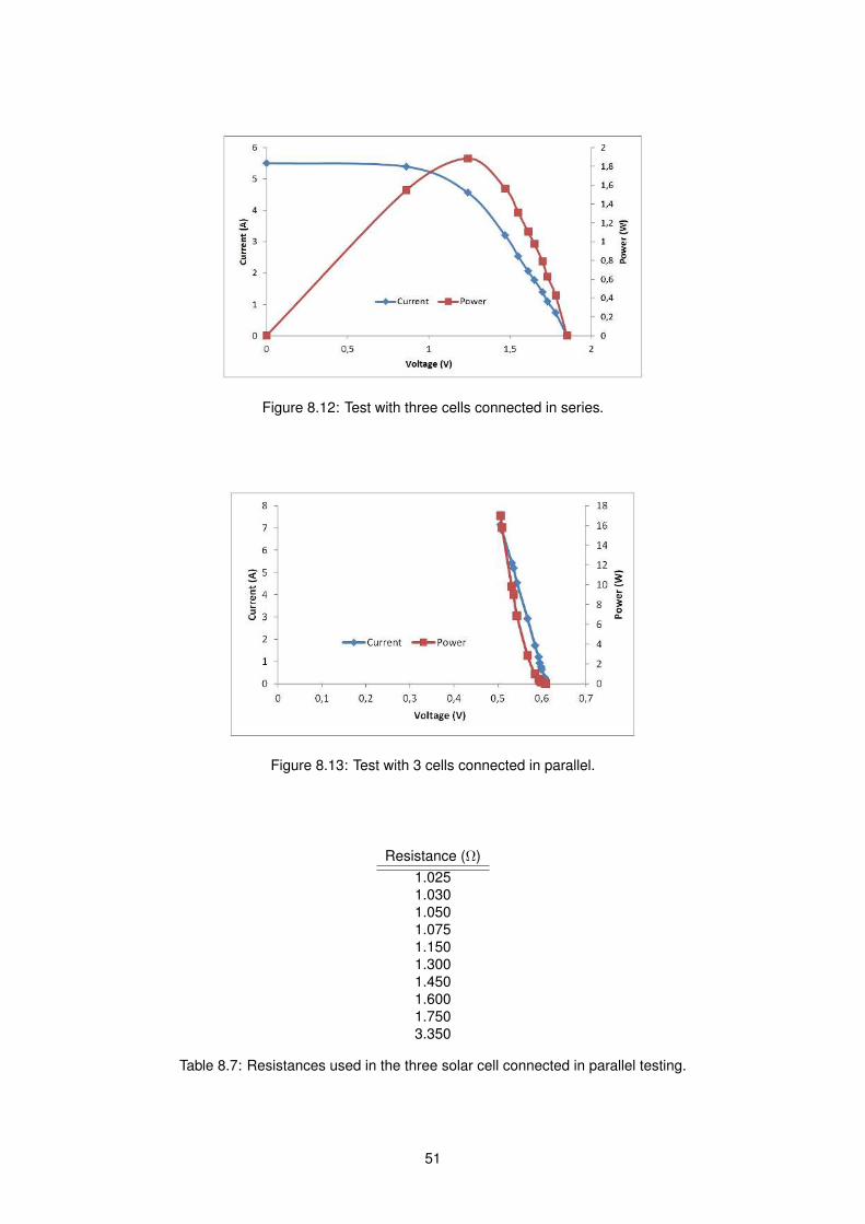
Figure 8.12: Test with three cells connected in series.
Figure 8.13: Test with 3 cells connected in parallel.
Resistance (Ω)
1.0251.0301.0501.0751.1501.3001.4501.6001.7503.350
Table 8.7: Resistances used in the three solar cell connected in parallel testing.
51
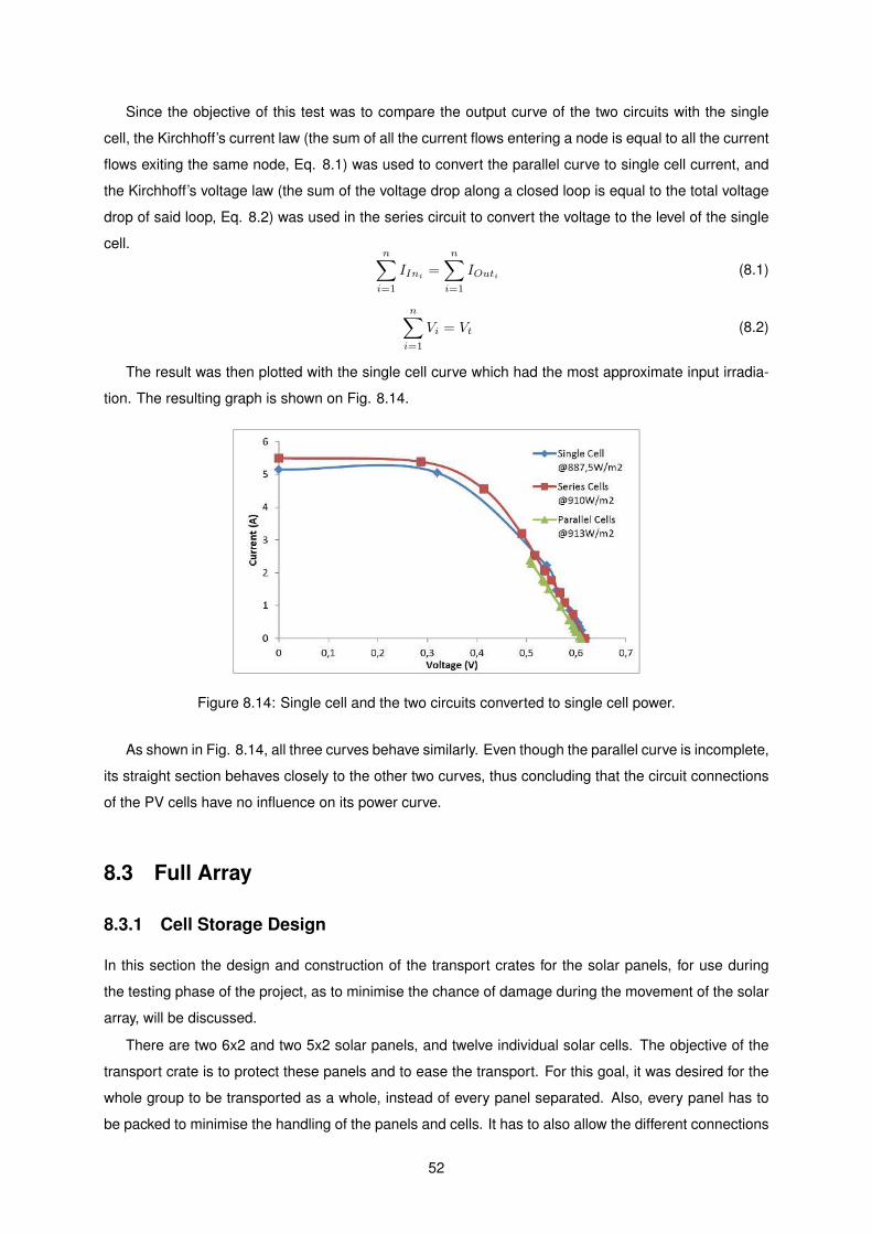
Since the objective of this test was to compare the output curve of the two circuits with the single
cell, the Kirchhoff’s current law (the sum of all the current flows entering a node is equal to all the current
flows exiting the same node, Eq. 8.1) was used to convert the parallel curve to single cell current, and
the Kirchhoff’s voltage law (the sum of the voltage drop along a closed loop is equal to the total voltage
drop of said loop, Eq. 8.2) was used in the series circuit to convert the voltage to the level of the single
cell.n∑
i=1
IIni=
n∑
i=1
IOuti (8.1)
n∑
i=1
Vi = Vt (8.2)
The result was then plotted with the single cell curve which had the most approximate input irradia-
tion. The resulting graph is shown on Fig. 8.14.
Figure 8.14: Single cell and the two circuits converted to single cell power.
As shown in Fig. 8.14, all three curves behave similarly. Even though the parallel curve is incomplete,
its straight section behaves closely to the other two curves, thus concluding that the circuit connections
of the PV cells have no influence on its power curve.
8.3 Full Array
8.3.1 Cell Storage Design
In this section the design and construction of the transport crates for the solar panels, for use during
the testing phase of the project, as to minimise the chance of damage during the movement of the solar
array, will be discussed.
There are two 6x2 and two 5x2 solar panels, and twelve individual solar cells. The objective of the
transport crate is to protect these panels and to ease the transport. For this goal, it was desired for the
whole group to be transported as a whole, instead of every panel separated. Also, every panel has to
be packed to minimise the handling of the panels and cells. It has to also allow the different connections
52
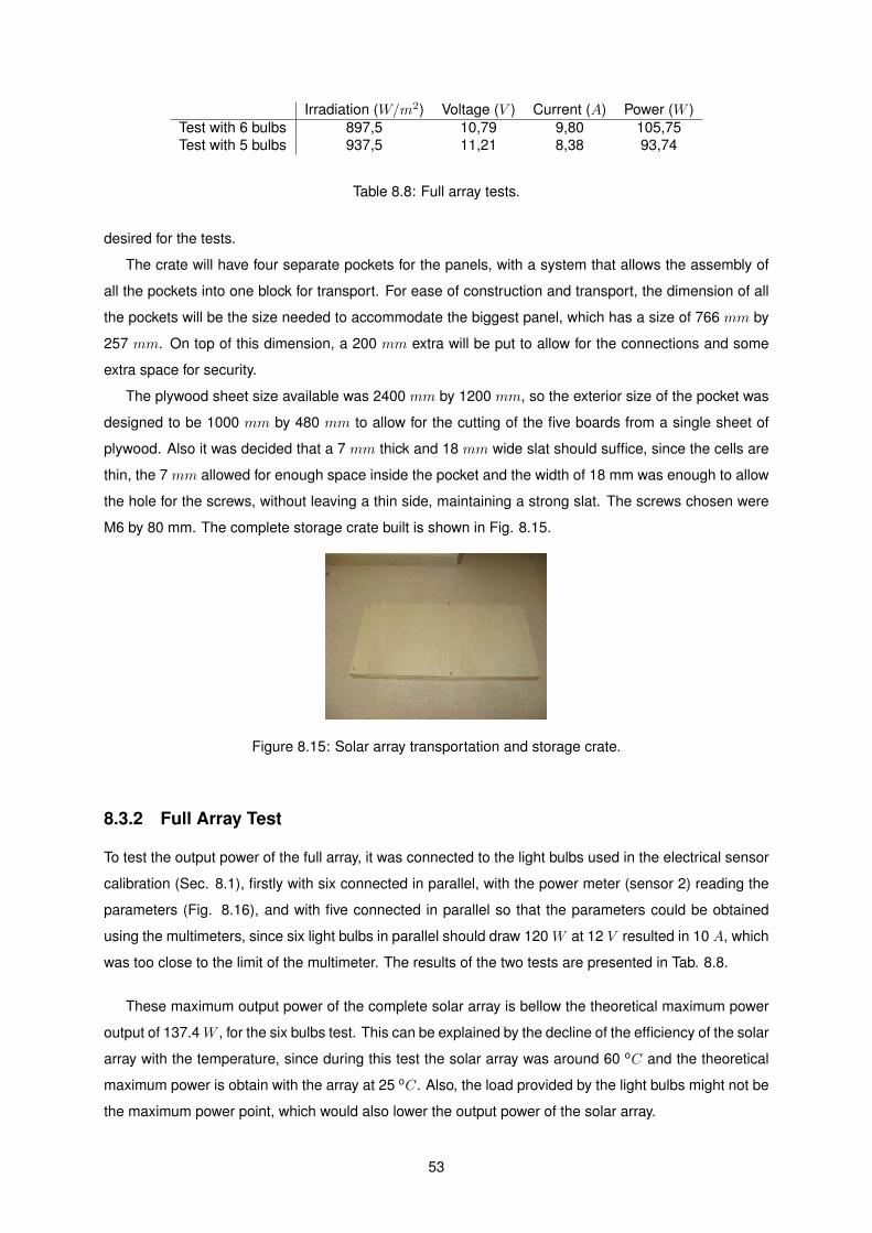
Irradiation (W/m2) Voltage (V ) Current (A) Power (W )
Test with 6 bulbs 897,5 10,79 9,80 105,75Test with 5 bulbs 937,5 11,21 8,38 93,74
Table 8.8: Full array tests.
desired for the tests.
The crate will have four separate pockets for the panels, with a system that allows the assembly of
all the pockets into one block for transport. For ease of construction and transport, the dimension of all
the pockets will be the size needed to accommodate the biggest panel, which has a size of 766 mm by
257 mm. On top of this dimension, a 200 mm extra will be put to allow for the connections and some
extra space for security.
The plywood sheet size available was 2400 mm by 1200 mm, so the exterior size of the pocket was
designed to be 1000 mm by 480 mm to allow for the cutting of the five boards from a single sheet of
plywood. Also it was decided that a 7 mm thick and 18 mm wide slat should suffice, since the cells are
thin, the 7 mm allowed for enough space inside the pocket and the width of 18 mm was enough to allow
the hole for the screws, without leaving a thin side, maintaining a strong slat. The screws chosen were
M6 by 80 mm. The complete storage crate built is shown in Fig. 8.15.
Figure 8.15: Solar array transportation and storage crate.
8.3.2 Full Array Test
To test the output power of the full array, it was connected to the light bulbs used in the electrical sensor
calibration (Sec. 8.1), firstly with six connected in parallel, with the power meter (sensor 2) reading the
parameters (Fig. 8.16), and with five connected in parallel so that the parameters could be obtained
using the multimeters, since six light bulbs in parallel should draw 120 W at 12 V resulted in 10 A, which
was too close to the limit of the multimeter. The results of the two tests are presented in Tab. 8.8.
These maximum output power of the complete solar array is bellow the theoretical maximum power
output of 137.4 W , for the six bulbs test. This can be explained by the decline of the efficiency of the solar
array with the temperature, since during this test the solar array was around 60 oC and the theoretical
maximum power is obtain with the array at 25 oC. Also, the load provided by the light bulbs might not be
the maximum power point, which would also lower the output power of the solar array.
53
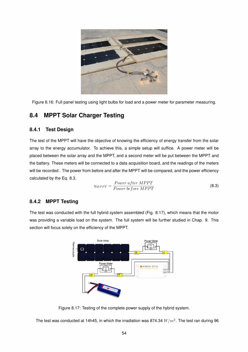
Figure 8.16: Full panel testing using light bulbs for load and a power meter for parameter measuring.
8.4 MPPT Solar Charger Testing
8.4.1 Test Design
The test of the MPPT will have the objective of knowing the efficiency of energy transfer from the solar
array to the energy accumulator. To achieve this, a simple setup will suffice. A power meter will be
placed between the solar array and the MPPT, and a second meter will be put between the MPPT and
the battery. These meters will be connected to a data acquisition board, and the readings of the meters
will be recorded . The power from before and after the MPPT will be compared, and the power efficiency
calculated by the Eq. 8.3.
ηMPPT =Power after MPPT
Power before MPPT(8.3)
8.4.2 MPPT Testing
The test was conducted with the full hybrid system assembled (Fig. 8.17), which means that the motor
was providing a variable load on the system. The full system will be further studied in Chap. 9. This
section will focus solely on the efficiency of the MPPT.
Figure 8.17: Testing of the complete power supply of the hybrid system.
The test was conducted at 14h45, in which the irradiation was 874.34 W/m2. The test ran during 96
54
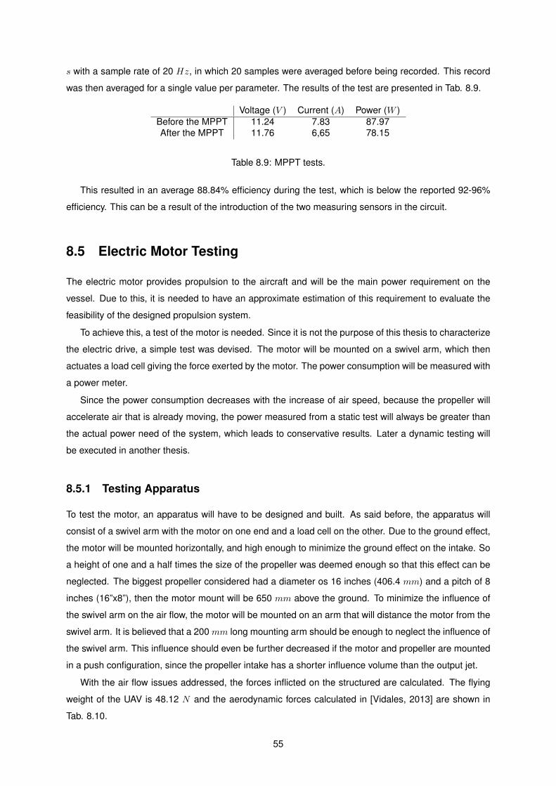
s with a sample rate of 20 Hz, in which 20 samples were averaged before being recorded. This record
was then averaged for a single value per parameter. The results of the test are presented in Tab. 8.9.
Voltage (V ) Current (A) Power (W )
Before the MPPT 11.24 7.83 87.97After the MPPT 11.76 6,65 78.15
Table 8.9: MPPT tests.
This resulted in an average 88.84% efficiency during the test, which is below the reported 92-96%
efficiency. This can be a result of the introduction of the two measuring sensors in the circuit.
8.5 Electric Motor Testing
The electric motor provides propulsion to the aircraft and will be the main power requirement on the
vessel. Due to this, it is needed to have an approximate estimation of this requirement to evaluate the
feasibility of the designed propulsion system.
To achieve this, a test of the motor is needed. Since it is not the purpose of this thesis to characterize
the electric drive, a simple test was devised. The motor will be mounted on a swivel arm, which then
actuates a load cell giving the force exerted by the motor. The power consumption will be measured with
a power meter.
Since the power consumption decreases with the increase of air speed, because the propeller will
accelerate air that is already moving, the power measured from a static test will always be greater than
the actual power need of the system, which leads to conservative results. Later a dynamic testing will
be executed in another thesis.
8.5.1 Testing Apparatus
To test the motor, an apparatus will have to be designed and built. As said before, the apparatus will
consist of a swivel arm with the motor on one end and a load cell on the other. Due to the ground effect,
the motor will be mounted horizontally, and high enough to minimize the ground effect on the intake. So
a height of one and a half times the size of the propeller was deemed enough so that this effect can be
neglected. The biggest propeller considered had a diameter os 16 inches (406.4 mm) and a pitch of 8
inches (16”x8”), then the motor mount will be 650 mm above the ground. To minimize the influence of
the swivel arm on the air flow, the motor will be mounted on an arm that will distance the motor from the
swivel arm. It is believed that a 200 mm long mounting arm should be enough to neglect the influence of
the swivel arm. This influence should even be further decreased if the motor and propeller are mounted
in a push configuration, since the propeller intake has a shorter influence volume than the output jet.
With the air flow issues addressed, the forces inflicted on the structured are calculated. The flying
weight of the UAV is 48.12 N and the aerodynamic forces calculated in [Vidales, 2013] are shown in
Tab. 8.10.
55
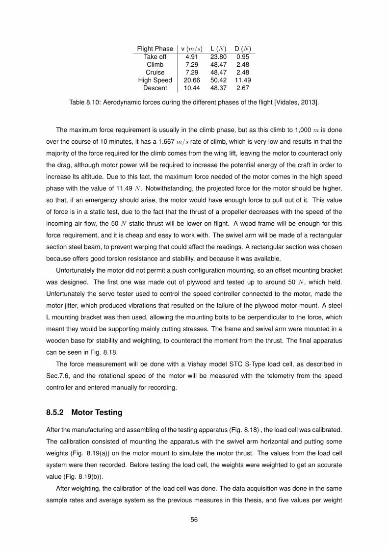
Flight Phase v (m/s) L (N ) D (N )
Take off 4.91 23.80 0.95Climb 7.29 48.47 2.48Cruise 7.29 48.47 2.48
High Speed 20.66 50.42 11.49Descent 10.44 48.37 2.67
Table 8.10: Aerodynamic forces during the different phases of the flight [Vidales, 2013].
The maximum force requirement is usually in the climb phase, but as this climb to 1,000 m is done
over the course of 10 minutes, it has a 1.667 m/s rate of climb, which is very low and results in that the
majority of the force required for the climb comes from the wing lift, leaving the motor to counteract only
the drag, although motor power will be required to increase the potential energy of the craft in order to
increase its altitude. Due to this fact, the maximum force needed of the motor comes in the high speed
phase with the value of 11.49 N . Notwithstanding, the projected force for the motor should be higher,
so that, if an emergency should arise, the motor would have enough force to pull out of it. This value
of force is in a static test, due to the fact that the thrust of a propeller decreases with the speed of the
incoming air flow, the 50 N static thrust will be lower on flight. A wood frame will be enough for this
force requirement, and it is cheap and easy to work with. The swivel arm will be made of a rectangular
section steel beam, to prevent warping that could affect the readings. A rectangular section was chosen
because offers good torsion resistance and stability, and because it was available.
Unfortunately the motor did not permit a push configuration mounting, so an offset mounting bracket
was designed. The first one was made out of plywood and tested up to around 50 N , which held.
Unfortunately the servo tester used to control the speed controller connected to the motor, made the
motor jitter, which produced vibrations that resulted on the failure of the plywood motor mount. A steel
L mounting bracket was then used, allowing the mounting bolts to be perpendicular to the force, which
meant they would be supporting mainly cutting stresses. The frame and swivel arm were mounted in a
wooden base for stability and weighting, to counteract the moment from the thrust. The final apparatus
can be seen in Fig. 8.18.
The force measurement will be done with a Vishay model STC S-Type load cell, as described in
Sec.7.6, and the rotational speed of the motor will be measured with the telemetry from the speed
controller and entered manually for recording.
8.5.2 Motor Testing
After the manufacturing and assembling of the testing apparatus (Fig. 8.18) , the load cell was calibrated.
The calibration consisted of mounting the apparatus with the swivel arm horizontal and putting some
weights (Fig. 8.19(a)) on the motor mount to simulate the motor thrust. The values from the load cell
system were then recorded. Before testing the load cell, the weights were weighted to get an accurate
value (Fig. 8.19(b)).
After weighting, the calibration of the load cell was done. The data acquisition was done in the same
sample rates and average system as the previous measures in this thesis, and five values per weight
56
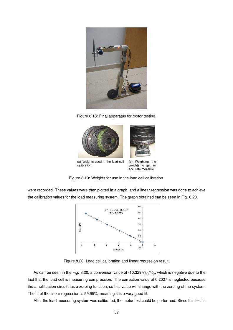
Figure 8.18: Final apparatus for motor testing.
(a) Weights used in the load cellcalibration.
(b) Weighting theweights to get anaccurate measure.
Figure 8.19: Weights for use in the load cell calibration.
were recorded. These values were then plotted in a graph, and a linear regression was done to achieve
the calibration values for the load measuring system. The graph obtained can be seen in Fig. 8.20.
Figure 8.20: Load cell calibration and linear regression result.
As can be seen in the Fig. 8.20, a conversion value of -10.329NM/VO, which is negative due to the
fact that the load cell is measuring compression. The correction value of 0.2037 is neglected because
the amplification circuit has a zeroing function, so this value will change with the zeroing of the system.
The fit of the linear regression is 99.95%, meaning it is a very good fit.
After the load measuring system was calibrated, the motor test could be performed. Since this test is
57
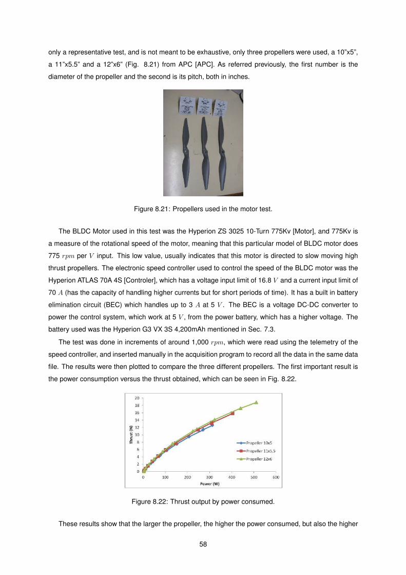
only a representative test, and is not meant to be exhaustive, only three propellers were used, a 10”x5”,
a 11”x5.5” and a 12”x6” (Fig. 8.21) from APC [APC]. As referred previously, the first number is the
diameter of the propeller and the second is its pitch, both in inches.
Figure 8.21: Propellers used in the motor test.
The BLDC Motor used in this test was the Hyperion ZS 3025 10-Turn 775Kv [Motor], and 775Kv is
a measure of the rotational speed of the motor, meaning that this particular model of BLDC motor does
775 rpm per V input. This low value, usually indicates that this motor is directed to slow moving high
thrust propellers. The electronic speed controller used to control the speed of the BLDC motor was the
Hyperion ATLAS 70A 4S [Controler], which has a voltage input limit of 16.8 V and a current input limit of
70 A (has the capacity of handling higher currents but for short periods of time). It has a built in battery
elimination circuit (BEC) which handles up to 3 A at 5 V . The BEC is a voltage DC-DC converter to
power the control system, which work at 5 V , from the power battery, which has a higher voltage. The
battery used was the Hyperion G3 VX 3S 4,200mAh mentioned in Sec. 7.3.
The test was done in increments of around 1,000 rpm, which were read using the telemetry of the
speed controller, and inserted manually in the acquisition program to record all the data in the same data
file. The results were then plotted to compare the three different propellers. The first important result is
the power consumption versus the thrust obtained, which can be seen in Fig. 8.22.
Figure 8.22: Thrust output by power consumed.
These results show that the larger the propeller, the higher the power consumed, but also the higher
58
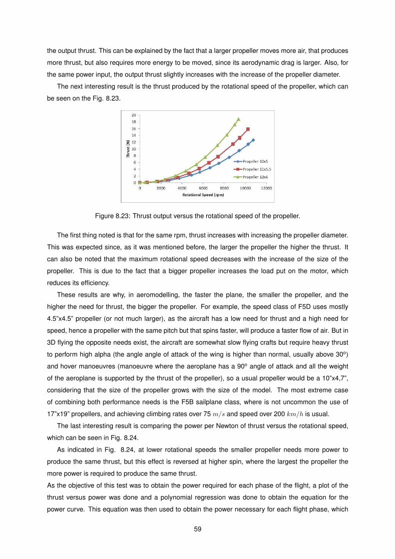
the output thrust. This can be explained by the fact that a larger propeller moves more air, that produces
more thrust, but also requires more energy to be moved, since its aerodynamic drag is larger. Also, for
the same power input, the output thrust slightly increases with the increase of the propeller diameter.
The next interesting result is the thrust produced by the rotational speed of the propeller, which can
be seen on the Fig. 8.23.
Figure 8.23: Thrust output versus the rotational speed of the propeller.
The first thing noted is that for the same rpm, thrust increases with increasing the propeller diameter.
This was expected since, as it was mentioned before, the larger the propeller the higher the thrust. It
can also be noted that the maximum rotational speed decreases with the increase of the size of the
propeller. This is due to the fact that a bigger propeller increases the load put on the motor, which
reduces its efficiency.
These results are why, in aeromodelling, the faster the plane, the smaller the propeller, and the
higher the need for thrust, the bigger the propeller. For example, the speed class of F5D uses mostly
4.5”x4.5” propeller (or not much larger), as the aircraft has a low need for thrust and a high need for
speed, hence a propeller with the same pitch but that spins faster, will produce a faster flow of air. But in
3D flying the opposite needs exist, the aircraft are somewhat slow flying crafts but require heavy thrust
to perform high alpha (the angle angle of attack of the wing is higher than normal, usually above 30o)
and hover manoeuvres (manoeuvre where the aeroplane has a 90o angle of attack and all the weight
of the aeroplane is supported by the thrust of the propeller), so a usual propeller would be a 10”x4,7”,
considering that the size of the propeller grows with the size of the model. The most extreme case
of combining both performance needs is the F5B sailplane class, where is not uncommon the use of
17”x19” propellers, and achieving climbing rates over 75 m/s and speed over 200 km/h is usual.
The last interesting result is comparing the power per Newton of thrust versus the rotational speed,
which can be seen in Fig. 8.24.
As indicated in Fig. 8.24, at lower rotational speeds the smaller propeller needs more power to
produce the same thrust, but this effect is reversed at higher spin, where the largest the propeller the
more power is required to produce the same thrust.
As the objective of this test was to obtain the power required for each phase of the flight, a plot of the
thrust versus power was done and a polynomial regression was done to obtain the equation for the
power curve. This equation was then used to obtain the power necessary for each flight phase, which
59
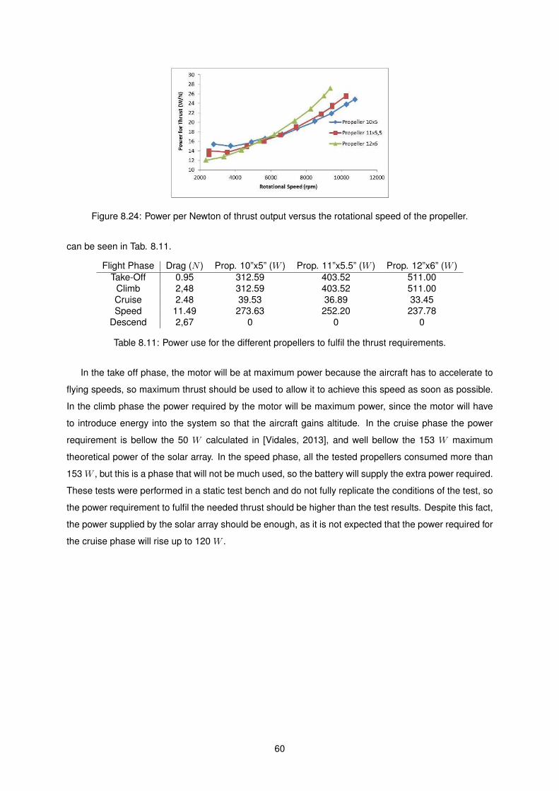
Figure 8.24: Power per Newton of thrust output versus the rotational speed of the propeller.
can be seen in Tab. 8.11.
Flight Phase Drag (N ) Prop. 10”x5” (W ) Prop. 11”x5.5” (W ) Prop. 12”x6” (W )
Take-Off 0.95 312.59 403.52 511.00Climb 2,48 312.59 403.52 511.00Cruise 2.48 39.53 36.89 33.45Speed 11.49 273.63 252.20 237.78
Descend 2,67 0 0 0
Table 8.11: Power use for the different propellers to fulfil the thrust requirements.
In the take off phase, the motor will be at maximum power because the aircraft has to accelerate to
flying speeds, so maximum thrust should be used to allow it to achieve this speed as soon as possible.
In the climb phase the power required by the motor will be maximum power, since the motor will have
to introduce energy into the system so that the aircraft gains altitude. In the cruise phase the power
requirement is bellow the 50 W calculated in [Vidales, 2013], and well bellow the 153 W maximum
theoretical power of the solar array. In the speed phase, all the tested propellers consumed more than
153 W , but this is a phase that will not be much used, so the battery will supply the extra power required.
These tests were performed in a static test bench and do not fully replicate the conditions of the test, so
the power requirement to fulfil the needed thrust should be higher than the test results. Despite this fact,
the power supplied by the solar array should be enough, as it is not expected that the power required for
the cruise phase will rise up to 120 W .
60

Chapter 9
Complete Hybrid Propulsion System
9.1 Complete System Hardware
For the full system testing, the two six by two solar panels and the two five by two panels mentioned
in Sec. 7.1 were connected to the MPPT referred in Sec. 7.2. This composed the energy generation
sub-system of the hybrid propulsion system. The energy accumulation sub-system was composed by a
Hyperion G3 VX 3S 4200mAh, as mentioned in Sec. 7.3. Finally the propulsion sub-system consisted
on the Hyperion ZS 3025 10-Turn 775Kv BLDC electric motor powering a APC 10”x5” propeller and
controlled by a Hyperion ATLAS 70A 4S ESC, as mentioned in Sec. 8.5.2. The propulsion sub-system
was mounted on the testing apparatus designed in Sec. sec:motortest. A schematic of the complete
hybrid system can be seen in Fig. 9.1.
Figure 9.1: Schematic of the complete hybrid propulsion system.
9.2 Hybrid Propulsion System Testing
For the complete test, the whole acquisition system was transported outside, to allow continuous acquisi-
tion of the various measuring sensors. The acquisition system was comprised of the SP215 pyranometer
61
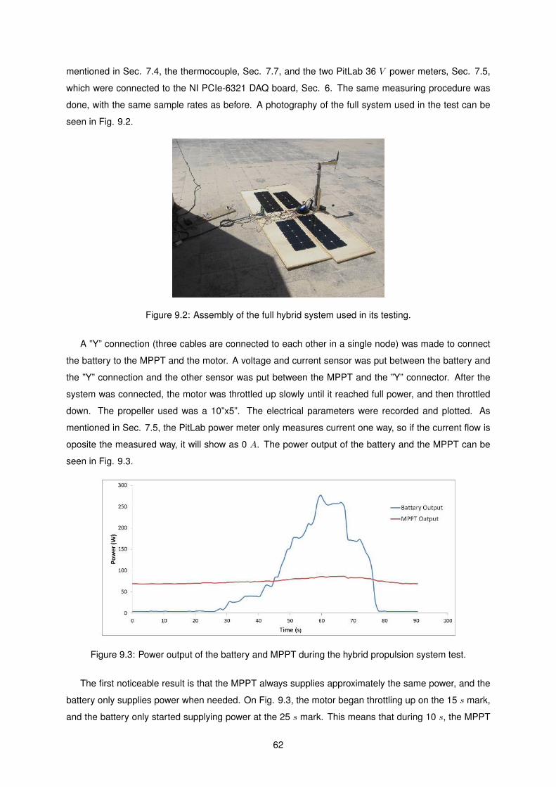
mentioned in Sec. 7.4, the thermocouple, Sec. 7.7, and the two PitLab 36 V power meters, Sec. 7.5,
which were connected to the NI PCIe-6321 DAQ board, Sec. 6. The same measuring procedure was
done, with the same sample rates as before. A photography of the full system used in the test can be
seen in Fig. 9.2.
Figure 9.2: Assembly of the full hybrid system used in its testing.
A ”Y” connection (three cables are connected to each other in a single node) was made to connect
the battery to the MPPT and the motor. A voltage and current sensor was put between the battery and
the ”Y” connection and the other sensor was put between the MPPT and the ”Y” connector. After the
system was connected, the motor was throttled up slowly until it reached full power, and then throttled
down. The propeller used was a 10”x5”. The electrical parameters were recorded and plotted. As
mentioned in Sec. 7.5, the PitLab power meter only measures current one way, so if the current flow is
oposite the measured way, it will show as 0 A. The power output of the battery and the MPPT can be
seen in Fig. 9.3.
Figure 9.3: Power output of the battery and MPPT during the hybrid propulsion system test.
The first noticeable result is that the MPPT always supplies approximately the same power, and the
battery only supplies power when needed. On Fig. 9.3, the motor began throttling up on the 15 s mark,
and the battery only started supplying power at the 25 s mark. This means that during 10 s, the MPPT
62
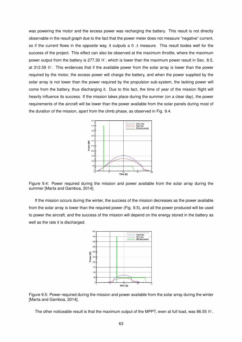
was powering the motor and the excess power was recharging the battery. This result is not directly
observable in the result graph due to the fact that the power meter does not measure ”negative” current,
so if the current flows in the opposite way, it outputs a 0 A measure. This result bodes well for the
success of the project. This effect can also be observed at the maximum throttle, where the maximum
power output from the battery is 277.30 W , which is lower than the maximum power result in Sec. 8.5,
at 312.59 W . This evidences that if the available power from the solar array is lower than the power
required by the motor, the excess power will charge the battery, and when the power supplied by the
solar array is not lower than the power required by the propulsion sub-system, the lacking power will
come from the battery, thus discharging it. Due to this fact, the time of year of the mission flight will
heavily influence its success. If the mission takes place during the summer (on a clear day), the power
requirements of the aircraft will be lower than the power available from the solar panels during most of
the duration of the mission, apart from the climb phase, as observed in Fig. 9.4.
Figure 9.4: Power required during the mission and power available from the solar array during thesummer [Marta and Gamboa, 2014].
If the mission occurs during the winter, the success of the mission decreases as the power available
from the solar array is lower than the required power (Fig. 9.5), and all the power produced will be used
to power the aircraft, and the success of the mission will depend on the energy stored in the battery as
well as the rate it is discharged.
Figure 9.5: Power required during the mission and power available from the solar array during the winter[Marta and Gamboa, 2014].
The other noticeable result is that the maximum output of the MPPT, even at full load, was 86.55 W ,
63
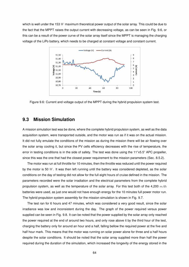
which is well under the 153 W maximum theoretical power output of the solar array. This could be due to
the fact that the MPPT raises the output current with decreasing voltage, as can be seen in Fig. 9.6, or
this can be a result of the power curve of the solar array itself since the MPPT is managing the charging
voltage of the LiPo battery, which needs to be charged at constant voltage and constant current.
Figure 9.6: Current and voltage output of the MPPT during the hybrid propulsion system test.
9.3 Mission Simulation
A mission simulation test was be done, where the complete hybrid propulsion system, as well as the data
acquisition system, were transported outside, and the motor was run as if it was on the actual mission.
It did not fully emulate the conditions of the mission as during the mission there will be air flowing over
the solar array cooling it, but since the PV cells efficiency decreases with the rise of temperature, the
error in testing conditions is in the side of safety. The test was done using the 11”x5.5” APC propeller,
since this was the one that had the closest power requirement to the mission parameters (Sec. 8.5.2).
The motor was run at full throttle for 10 minutes, then the throttle was reduced until the power required
by the motor is 50 W . It was then left running until the battery was considered depleted, as the solar
conditions on the day of testing did not allow for the full eight hours of cruise defined in the mission. The
parameters recorded were the solar irradiation and the electrical parameters from the complete hybrid
propulsion system, as well as the temperature of the solar array. For this test both of the 4,200 mAh
batteries were used, as just one would not have enough energy for the 10 minutes full power motor run.
The hybrid propulsion system assembly for the mission simulation is shown in Fig. 9.7.
The test ran for 6 hours and 47 minutes, which was considered a very good result, since the solar
irradiance was low and inconsistent during the day. The graph of the power required versus power
supplied can be seen in Fig. 9.8. It can be noted that the power supplied by the solar array only reached
the power required at the end of around two hours, and only rose above it by the third hour of the test,
charging the battery only for around an hour and a half, falling bellow the required power at the five and
half hour mark. This means that the motor was running on solar power alone for three and a half hours
despite the solar conditions. It should be noted that the solar array supplied more than half the power
required during the duration of the simulation, which increased the longevity of the energy stored in the
64
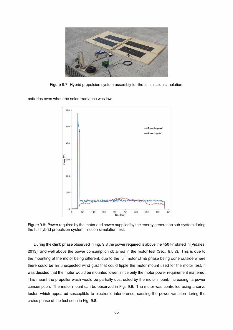
Figure 9.7: Hybrid propulsion system assembly for the full mission simulation.
batteries even when the solar irradiance was low.
Figure 9.8: Power required by the motor and power supplied by the energy generation sub-system duringthe full hybrid propulsion system mission simulation test.
During the climb phase observed in Fig. 9.8 the power required is above the 450 W stated in [Vidales,
2013], and well above the power consumption obtained in the motor test (Sec. 8.5.2). This is due to
the mounting of the motor being different, due to the full motor climb phase being done outside where
there could be an unexpected wind gust that could tipple the motor mount used for the motor test, it
was decided that the motor would be mounted lower, since only the motor power requirement mattered.
This meant the propeller wash would be partially obstructed by the motor mount, increasing its power
consumption. The motor mount can be observed in Fig. 9.9. The motor was controlled using a servo
tester, which appeared susceptible to electronic interference, causing the power variation during the
cruise phase of the test seen in Fig. 9.8.
65
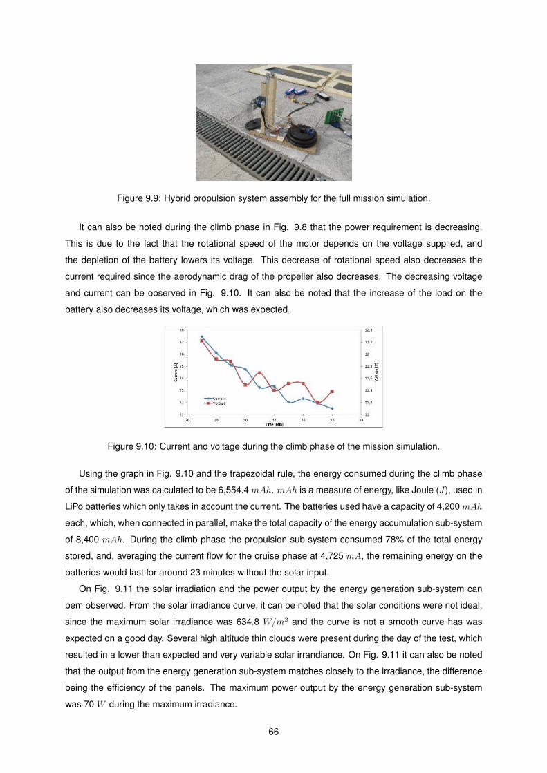
Figure 9.9: Hybrid propulsion system assembly for the full mission simulation.
It can also be noted during the climb phase in Fig. 9.8 that the power requirement is decreasing.
This is due to the fact that the rotational speed of the motor depends on the voltage supplied, and
the depletion of the battery lowers its voltage. This decrease of rotational speed also decreases the
current required since the aerodynamic drag of the propeller also decreases. The decreasing voltage
and current can be observed in Fig. 9.10. It can also be noted that the increase of the load on the
battery also decreases its voltage, which was expected.
Figure 9.10: Current and voltage during the climb phase of the mission simulation.
Using the graph in Fig. 9.10 and the trapezoidal rule, the energy consumed during the climb phase
of the simulation was calculated to be 6,554.4 mAh. mAh is a measure of energy, like Joule (J), used in
LiPo batteries which only takes in account the current. The batteries used have a capacity of 4,200 mAh
each, which, when connected in parallel, make the total capacity of the energy accumulation sub-system
of 8,400 mAh. During the climb phase the propulsion sub-system consumed 78% of the total energy
stored, and, averaging the current flow for the cruise phase at 4,725 mA, the remaining energy on the
batteries would last for around 23 minutes without the solar input.
On Fig. 9.11 the solar irradiation and the power output by the energy generation sub-system can
bem observed. From the solar irradiance curve, it can be noted that the solar conditions were not ideal,
since the maximum solar irradiance was 634.8 W/m2 and the curve is not a smooth curve has was
expected on a good day. Several high altitude thin clouds were present during the day of the test, which
resulted in a lower than expected and very variable solar irrandiance. On Fig. 9.11 it can also be noted
that the output from the energy generation sub-system matches closely to the irradiance, the difference
being the efficiency of the panels. The maximum power output by the energy generation sub-system
was 70 W during the maximum irradiance.
66
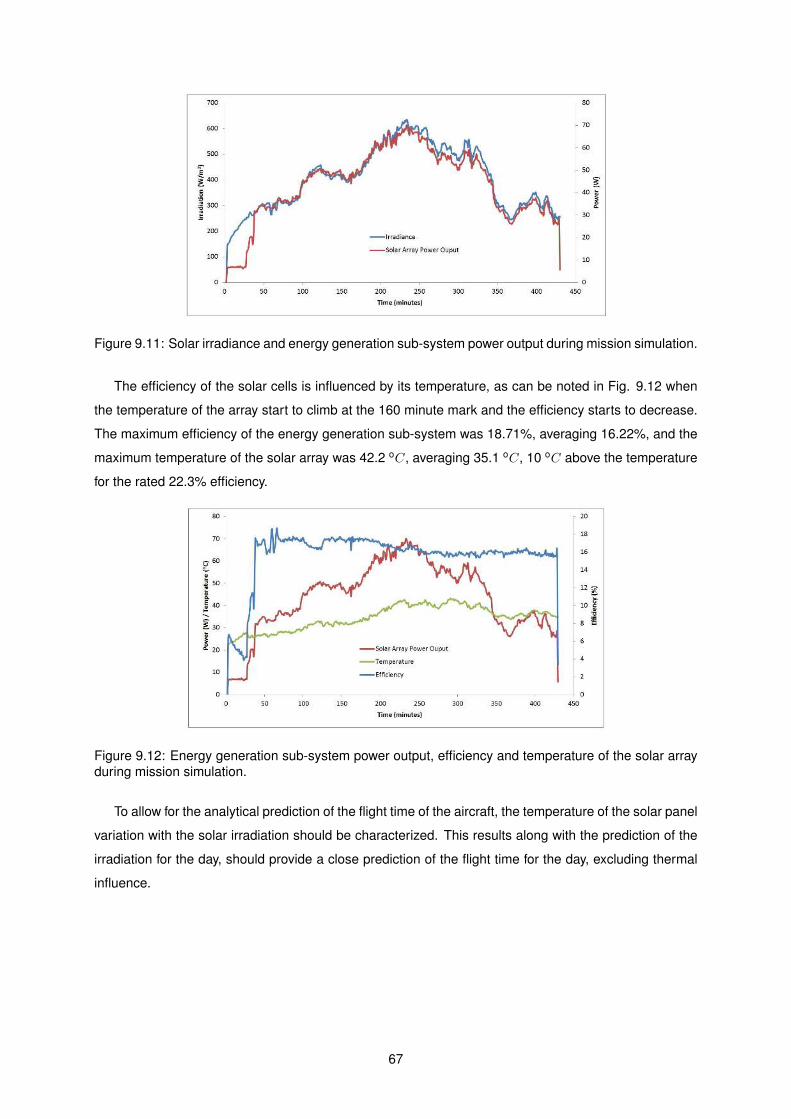
Figure 9.11: Solar irradiance and energy generation sub-system power output during mission simulation.
The efficiency of the solar cells is influenced by its temperature, as can be noted in Fig. 9.12 when
the temperature of the array start to climb at the 160 minute mark and the efficiency starts to decrease.
The maximum efficiency of the energy generation sub-system was 18.71%, averaging 16.22%, and the
maximum temperature of the solar array was 42.2 oC, averaging 35.1 oC, 10 oC above the temperature
for the rated 22.3% efficiency.
Figure 9.12: Energy generation sub-system power output, efficiency and temperature of the solar arrayduring mission simulation.
To allow for the analytical prediction of the flight time of the aircraft, the temperature of the solar panel
variation with the solar irradiation should be characterized. This results along with the prediction of the
irradiation for the day, should provide a close prediction of the flight time for the day, excluding thermal
influence.
67

68

Chapter 10
Heat Shrink Film Test
Due to the fact that the wing skin is a heat shrinking film, that will have to support the solar cell array,
which is comprised of dark grey coloured solar cells, some problems of warping can occur on the wing
because the solar cells will heat up, causing a rise in temperature of only the top skin, as the bottom
skin will be in the shadow of the solar array. This temperature rise could cause the contraction of the
top skin, which could warp the wing, changing the flight characteristics, that could cause the crash of
the model. The heat shrinking film used was the trans yellow film from Solarfilm [Solarfilm], since both
colours of the film should exhibit the same behaviour.
10.1 Testing Apparatus
To better understand the behaviour of this film, a testing apparatus was designed. The device was
designed to allow the assembly of a solar cell on top of a strip of film, although the characterization will
be done with a more controllable heat source.
The apparatus was designed to measure the load due to the shrinking film when subjected to a heat
source, and the amount of heat needed to develop such load. The testing apparatus also had to have
enough space to allow the mounting of a solar cell on top of the film, in order to simulate the working
conditions it will be subjected.
To measure the load, a strain gauge was used. This strain gauge could be applied directly on the
film, so only a simple frame to hold the film would be needed. But, since the strain gauge measures the
strain and not the load, the film’s Young’s modulus would have to be known. Since this data is not known,
and the testing for this would take additional resources, the apparatus was made so that the strain gauge
would be applied to a material which the Young’s modulus is known. For this reason, the testing device
was a frame, where the film was fixed on one side of the frame, and the other side was fixed to a moving
bar that is hold by a metal sheet, which had the strain gauge mounted on to it to measure it’s strain,
making a simple load cell. Due to the low forces involved (around 50N are expected), the metal for
the load cell will have be as pliable and thin as possible. The metal would also have to be cheap and
available, so aluminium was chosen.
69
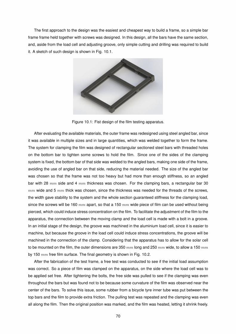
The first approach to the design was the easiest and cheapest way to build a frame, so a simple bar
frame frame held together with screws was designed. In this design, all the bars have the same section,
and, aside from the load cell and adjusting groove, only simple cutting and drilling was required to build
it. A sketch of such design is shown in Fig. 10.1.
Figure 10.1: Fist design of the film testing apparatus.
After evaluating the available materials, the outer frame was redesigned using steel angled bar, since
it was available in multiple sizes and in large quantities, which was welded together to form the frame.
The system for clamping the film was designed of rectangular sectioned steel bars with threaded holes
on the bottom bar to tighten some screws to hold the film. Since one of the sides of the clamping
system is fixed, the bottom bar of that side was welded to the angled bars, making one side of the frame,
avoiding the use of angled bar on that side, reducing the material needed. The size of the angled bar
was chosen so that the frame was not too heavy but had more than enough stiffness, so an angled
bar with 28 mm side and 4 mm thickness was chosen. For the clamping bars, a rectangular bar 30
mm wide and 5 mm thick was chosen, since the thickness was needed for the threads of the screws,
the width gave stability to the system and the whole section guaranteed stiffness for the clamping load,
since the screws will be 160 mm apart, so that a 150 mm wide piece of film can be used without being
pierced, which could induce stress concentration on the film. To facilitate the adjustment of the film to the
apparatus, the connection between the moving clamp and the load cell is made with a bolt in a groove.
In an initial stage of the design, the groove was machined in the aluminium load cell, since it is easier to
machine, but because the groove in the load cell could induce stress concentrations, the groove will be
machined in the connection of the clamp. Considering that the apparatus has to allow for the solar cell
to be mounted on the film, the outer dimensions are 350 mm long and 250 mm wide, to allow a 150 mm
by 150 mm free film surface. The final geometry is shown in Fig. 10.2.
After the fabrication of the test frame, a free test was conducted to see if the initial load assumption
was correct. So a piece of film was clamped on the apparatus, on the side where the load cell was to
be applied set free. After tightening the bolts, the free side was pulled to see if the clamping was even
throughout the bars but was found not to be because some curvature of the film was observed near the
center of the bars. To solve this issue, some rubber from a bicycle tyre inner tube was put between the
top bars and the film to provide extra friction. The pulling test was repeated and the clamping was even
all along the film. Then the original position was marked, and the film was heated, letting it shrink freely.
70
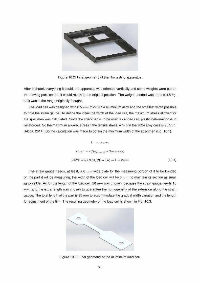
Figure 10.2: Final geometry of the film testing apparatus.
After it shrank everything it could, the apparatus was oriented vertically and some weights were put on
the moving part, so that it would return to the original position. The weight needed was around 4.5 kg,
so it was in the range originally thought.
The load cell was designed with 0.5 mm thick 2024 aluminium alloy and the smallest width possible
to hold the strain gauge. To define the initial the width of the load cell, the maximum stress allowed for
the specimen was calculated. Since the specimen is to be used as a load cell, plastic deformation is to
be avoided. So the maximum allowed stress it the tensile stress, which in the 2024 alloy case is 96MPa
[Alcoa, 2014]. So the calculation was made to obtain the minimum width of the specimen (Eq. 10.1).
F = σ ∗ area
width = F/(σallowed ∗ thickness)
width = 5 ∗ 9.81/(96 ∗ 0.5) = 1, 308mm (10.1)
The strain gauge needs, at least, a 6 mm wide plate for the measuring portion of it to be bonded
on the part it will be measuring, the width of the load cell will be 6 mm, to maintain its section as small
as possible. As for the length of the load cell, 20 mm was chosen, because the strain gauge needs 16
mm, and the extra length was chosen to guarantee the homogeneity of the extension along the strain
gauge. The total length of the part is 95 mm to accommodate the gradual width variation and the length
for adjustment of the film. The resulting geometry of the load cell is shown in Fig. 10.3.
Figure 10.3: Final geometry of the aluminium load cell.
71
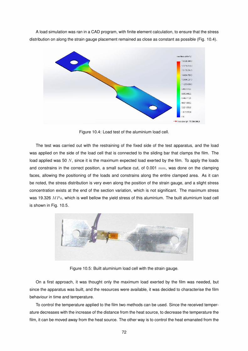
A load simulation was ran in a CAD program, with finite element calculation, to ensure that the stress
distribution on along the strain gauge placement remained as close as constant as possible (Fig. 10.4).
Figure 10.4: Load test of the aluminium load cell.
The test was carried out with the restraining of the fixed side of the test apparatus, and the load
was applied on the side of the load cell that is connected to the sliding bar that clamps the film. The
load applied was 50 N , since it is the maximum expected load exerted by the film. To apply the loads
and constrains in the correct position, a small surface cut, of 0.001 mm, was done on the clamping
faces, allowing the positioning of the loads and constrains along the entire clamped area. As it can
be noted, the stress distribution is very even along the position of the strain gauge, and a slight stress
concentration exists at the end of the section variation, which is not significant. The maximum stress
was 19.326 MPa, which is well bellow the yield stress of this aluminium. The built aluminium load cell
is shown in Fig. 10.5.
Figure 10.5: Built aluminium load cell with the strain gauge.
On a first approach, it was thought only the maximum load exerted by the film was needed, but
since the apparatus was built, and the resources were available, it was decided to characterise the film
behaviour in time and temperature.
To control the temperature applied to the film two methods can be used. Since the received temper-
ature decreases with the increase of the distance from the heat source, to decrease the temperature the
film, it can be moved away from the heat source. The other way is to control the heat emanated from the
72
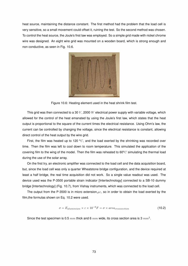
heat source, maintaining the distance constant. The first method had the problem that the load cell is
very sensitive, so a small movement could offset it, ruining the test. So the second method was chosen.
To control the heat source, the Joule’s first law was employed. So a simple grid made with nickel chrome
wire was designed. An eight wire grid was mounted on a wooden board, which is strong enough and
non conductive, as seen in Fig. 10.6.
Figure 10.6: Heating element used in the heat shrink film test.
This grid was then connected to a 30 V , 2000 W electrical power supply with variable voltage, which
allowed for the control of the heat emanated by using the Joule’s first law, which states that the heat
output is proportional to the square of the current times the electrical resistance. Using Ohm’s law, the
current can be controlled by changing the voltage, since the electrical resistance is constant, allowing
direct control of the heat output by the wire grid.
First, the film was heated up to 120 oC, and the load exerted by the shrinking was recorded over
time. Then the film was left to cool down to room temperature. This simulated the application of the
covering film to the wing of the model. Then the film was reheated to 60oC simulating the thermal load
during the use of the solar array.
On the first try, an electronic amplifier was connected to the load cell and the data acquisition board,
but, since the load cell was only a quarter Wheatstone bridge configuration, and the device required at
least a half bridge, the real time acquisition did not work. So a single value readout was used. The
device used was the P-3500 portable strain indicator [Intertechnology] connected to a SB-10 dummy
bridge [Intertechnology] (Fig. 10.7), from Vishay instruments, which was connected to the load cell.
The output from the P-3500 is in micro extension,µε, so in order to obtain the load exerted by the
film,the formulas shown on Eq. 10.2 were used.
σ = Ealuminium × ε× 10−6F = σ × areacrosssection (10.2)
Since the test specimen is 0.5 mm thick and 6 mm wide, its cross section area is 3 mm2.
73
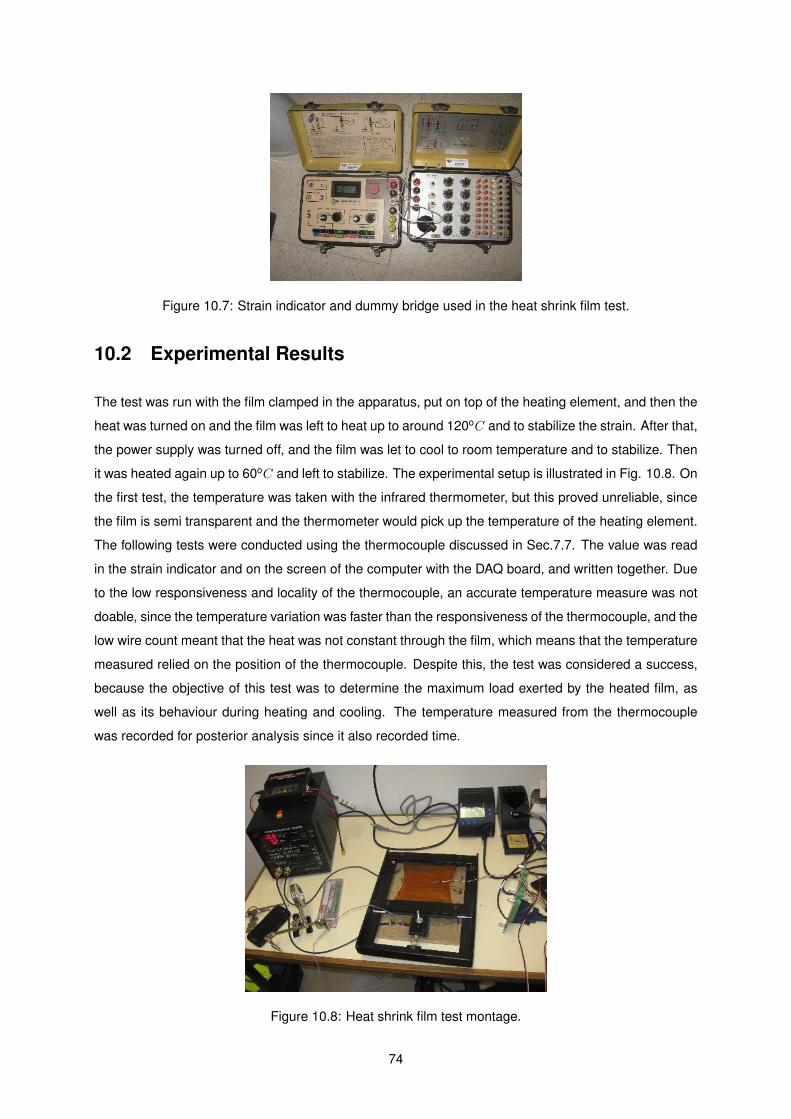
Figure 10.7: Strain indicator and dummy bridge used in the heat shrink film test.
10.2 Experimental Results
The test was run with the film clamped in the apparatus, put on top of the heating element, and then the
heat was turned on and the film was left to heat up to around 120oC and to stabilize the strain. After that,
the power supply was turned off, and the film was let to cool to room temperature and to stabilize. Then
it was heated again up to 60oC and left to stabilize. The experimental setup is illustrated in Fig. 10.8. On
the first test, the temperature was taken with the infrared thermometer, but this proved unreliable, since
the film is semi transparent and the thermometer would pick up the temperature of the heating element.
The following tests were conducted using the thermocouple discussed in Sec.7.7. The value was read
in the strain indicator and on the screen of the computer with the DAQ board, and written together. Due
to the low responsiveness and locality of the thermocouple, an accurate temperature measure was not
doable, since the temperature variation was faster than the responsiveness of the thermocouple, and the
low wire count meant that the heat was not constant through the film, which means that the temperature
measured relied on the position of the thermocouple. Despite this, the test was considered a success,
because the objective of this test was to determine the maximum load exerted by the heated film, as
well as its behaviour during heating and cooling. The temperature measured from the thermocouple
was recorded for posterior analysis since it also recorded time.
Figure 10.8: Heat shrink film test montage.
74
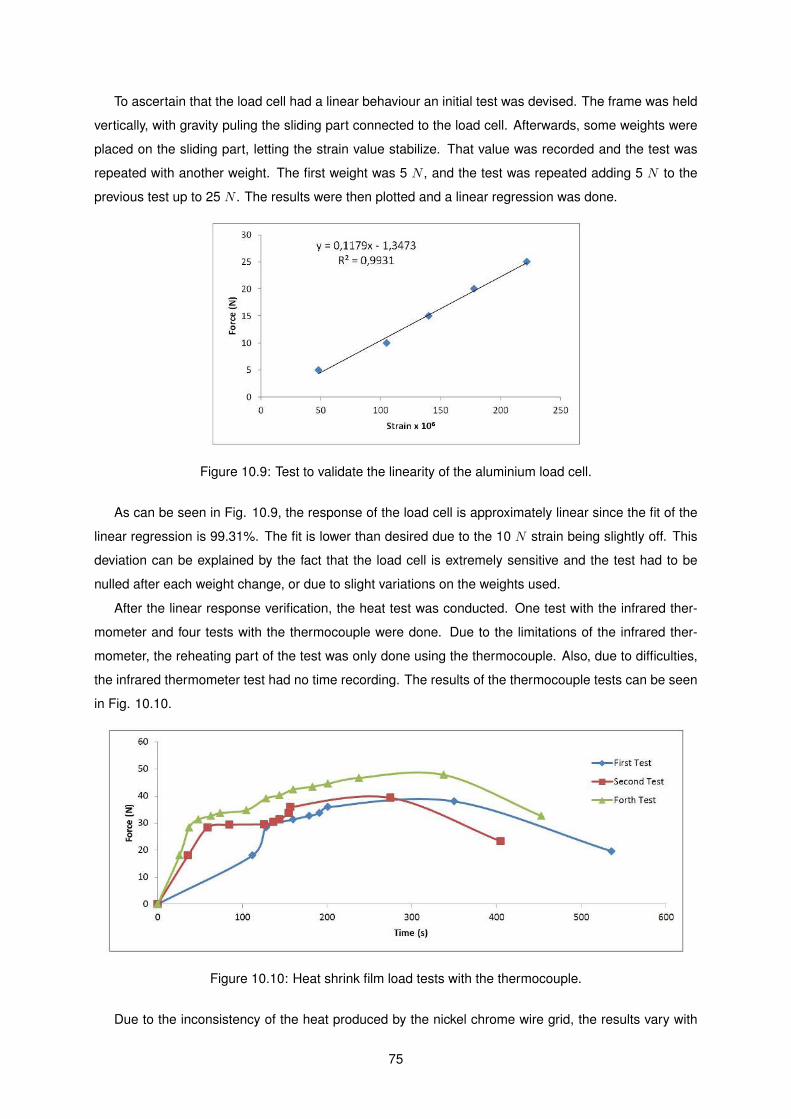
To ascertain that the load cell had a linear behaviour an initial test was devised. The frame was held
vertically, with gravity puling the sliding part connected to the load cell. Afterwards, some weights were
placed on the sliding part, letting the strain value stabilize. That value was recorded and the test was
repeated with another weight. The first weight was 5 N , and the test was repeated adding 5 N to the
previous test up to 25 N . The results were then plotted and a linear regression was done.
Figure 10.9: Test to validate the linearity of the aluminium load cell.
As can be seen in Fig. 10.9, the response of the load cell is approximately linear since the fit of the
linear regression is 99.31%. The fit is lower than desired due to the 10 N strain being slightly off. This
deviation can be explained by the fact that the load cell is extremely sensitive and the test had to be
nulled after each weight change, or due to slight variations on the weights used.
After the linear response verification, the heat test was conducted. One test with the infrared ther-
mometer and four tests with the thermocouple were done. Due to the limitations of the infrared ther-
mometer, the reheating part of the test was only done using the thermocouple. Also, due to difficulties,
the infrared thermometer test had no time recording. The results of the thermocouple tests can be seen
in Fig. 10.10.
Figure 10.10: Heat shrink film load tests with the thermocouple.
Due to the inconsistency of the heat produced by the nickel chrome wire grid, the results vary with
75
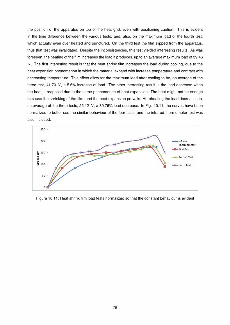
the position of the apparatus on top of the heat grid, even with positioning caution. This is evident
in the time difference between the various tests, and, also, on the maximum load of the fourth test,
which actually even over heated and punctured. On the third test the film slipped from the apparatus,
thus that test was invalidated. Despite the inconsistencies, this test yielded interesting results. As was
foreseen, the heating of the film increases the load it produces, up to an average maximum load of 39.46
N . The first interesting result is that the heat shrink film increases the load during cooling, due to the
heat expansion phenomenon in which the material expand with increase temperature and contract with
decreasing temperature. This effect allow for the maximum load after cooling to be, on average of the
three test, 41.70 N , a 5.6% increase of load. The other interesting result is the load decrease when
the heat is reapplied due to the same phenomenon of heat expansion. The heat might not be enough
to cause the shrinking of the film, and the heat expansion prevails. At reheating the load decreases to,
on average of the three tests, 25.12 N , a 39.76% load decrease. In Fig. 10.11, the curves have been
normalized to better see the similar behaviour of the four tests, and the infrared thermometer test was
also included.
Figure 10.11: Heat shrink film load tests normalized so that the constant behaviour is evident
76
Chapter 11
Conclusions
11.1 Achievements
The objective of this thesis was to design and evaluate a hybrid propulsion system for a long endurance
electric unmanned aerial vehicle (UAV). For the accomplishment of this objective, the mission objectives
and requirements were defined and explained, and a UAV design was proposed and evaluated. The
performance of this UAV was then used to calculate the required energy requirements for the successful
completion of the mission.
A hybrid system comprised of photovoltaic solar cells (PV cells), assembled in an array, and a lithium
polymer (LiPo) battery was deemed the best solution, since the LiPo battery has a high energy density
(can accumulate large amounts of energy for its weight), and the large area available on the wings are
a suitable place to mount a solar array of sufficient capacity to supply energy during the cruise phase of
the mission. To verify the validity of this system, several tests were conducted.
To conduct these tests some sensors had to be acquired. The choice was to use a voltage and
current sensor, used in several first person view (FPV) systems, for the electrical measurements, a
thermocouple to measure temperature, and a photodiode pyranometer for the energy irradiated on to
the solar cells.
The first test focused on the individual cells, to validate the load curve supplied by the manufacturer,
using variable loads, using resistors, to create the load curve. The result curve was closely matched
with the supplied curve, the main difference being the input energy and the temperature of the cells,
since this was an outdoor and unregulated test. The test was repeated with different PV cell circuits to
verify the curve characteristics remained with different PV cell configurations. The next test was to test
the individual cell with energy input variations by changing the angle of incidence of the light on the cell,
in which an energy gain was achieved, and using the UAV covering film over the cell, which resulted in
energy output losses. The tilting test resulted in an average 17.15% increase in power output during the
45 o test. The covering film test resulted in an average decrease of 34.4% and 7% power losses during
the yellow and transparent films test, respectively. This result led to the conclusion that the solar cells
should be mounted on the outside of the wing, despite the aerodynamic losses incurred, the energy
77
generation gains should be higher than the aerodynamic losses.
A full array test was then conducted, using a resistor load, rated for maximum 120 W , to verify the
maximum power the array could supply, and it achieved 105.75 W . Then the full array was connected
to the rest of the hybrid system, the MPPT, the battery and the motor. During this test the efficiency of
the MPPT and the operation of the full system were studied. The MPPT achieved a 88.84% average
efficiency. The full system worked in a surprising way, where energy would only be drawn from the
battery when the needed power required exceeded the MPPT output, and the power output from the
MPPT varied with the voltage of the battery, so the more depleted the battery the higher the output of
the MPPT.
In the final test, the solar conditions were not ideal, since the day was late in the year, and high
thin clouds were present. Despite this, the full hybrid propulsion mission simulation ran for 6 hours 47
minutes, in which the energy generation sub-system supplied over half of the required power during the
cruise phase, full supplying during three and a half hours and charging the battery during an hour and a
half during that time, having a maximum output of 70 W . During the climb phase simulation, the power
requirement was higher than 450 W due to changes in the motor mount, consuming 6,554.4 mAh, 78%
of the available 8,400 mAh. The maximum irradiance during the day was 634.8 W/m2 and the energy
generation sub-system had an average efficiency of 16.22% at an average temperature of 35.1 oC. In
conclusion, if the conditions during the day had been a bit better, the eight hour cruise would have been
accomplished, so the mission would be a success since the higher altitude and lower temperature, allied
with the lower power consumption during climb, would mean that the solar array would be more efficient
and the batteries would have more energy stored for the flight. To allow the prediction of the flight time
of the mission a in depth characterization of the temperature and efficiency of the solar panels variation
with the solar radiation should be done. This should allow for a close prediction of the flight time knowing
only the predicted irradiation for the day of the flight, since the majority of the other variables, like the
energy available in the batteries and the energy spent by the motor are know..
Due to the construction method of the UAV, heat shrinking film over a balsa frame, and the heating
characteristic of the solar array, a test on the behaviour of the covering film was conducted to ascertain
the viability of the mounting of the solar array on the wings, since some contraction or relaxation of the
top cover, where the array would be mounted, could significantly change the flight characteristics of the
aircraft. For this purpose of testing the film, a steel frame and aluminium load cell were designed and
built. A heating element was also designed and build to enable the control of the heat applied to the
film while keeping the frame still, due to the sensitivity of the load cell. The behaviour of the film was
unexpected since the film would contract during the heating phase, and continue to contract after the
heat was turned off, but when heat was reapplied, it would extend. The conclusion derived from these
results is that further test should be done since the warping of the wing is not intuitive. The relaxation of
the top cover film can be a good thing, since this relaxation promotes the decrease of the dihedral of the
wing, counteracting the lift force on the wings, decreasing the bending of the wing. On the other side,
decreasing the dihedral of the wing also decreases the rolling stability of the UAV. Besides decreasing
the dihedral, some warping of the wing can also occur, which could change the flight characteristics,
78

mainly drag and stall characteristics, which could significantly affect the mission.
11.2 Future Work
In the future, a better and more accurate test of the motor will be done. This will allow the choice of the
best motor and propeller combination for the flight envelope of the mission. This test will be done in a
wind tunnel, which will allow the closer simulation of the flight variables.
As for the system assembly, a partially built wing with a heating element under the skin should be put
on the wind tunnel to ascertain the temperature of the film with the airflow, and to determine if the warp
of the wing is significant enough to change the flight characteristics of the UAV. If this proves true, a new
method of building the wings may prove needed, or a different way to mount the solar array on the wing
to reduce the heat transfer.
79

80

Bibliography
AEROG. Aeronautics and Astronautics Research Center. http://www.idmec.ist.utl.pt/laeta/,
2014. Acessed in September.
Alcoa. http://www.alcoa.com/mill_products/catalog/pdf/alloy2024techsheet.pdf, 2014.
Acessed in May.
I. Alphonse, D. S. HosiminThilagar, and F. B. Singh. Design of solar powered bldc motor driven electric
vehicle. International Journal of Renewable Energy Research, 2(3), 2012.
AnyVolt. https://www.dimensionengineering.com/products/anyvolt-micro. Acessed in March
2014.
APC. http://www.apcprop.com/v/index.html. Acessed in March 2014.
Apogee. http://www.apogeeinstruments.co.uk/amplified-0-5-volt-pyranometer-sp-215/,
2014. Acessed in June.
R. J. Boucher. Hystory of solar flight. AIAA Paper, pages 84–1429, 1984.
CCTAE. Center of Aeronautical and Space Science and Technology. https://fenix.tecnico.
ulisboa.pt/investigacao/cctae, 2014. Acessed in September.
N. Centurion. http://www.nasa.gov/centers/dryden/history/pastprojects/Erast/centurion2.
html#.VClGWvldWHU. Acessed in September 2014.
M. K. Chawla. A step by step guide to selecting the ”right” Solar Simulator for your solar cell testing
application. Photo Emission Tech. Inc.
H. S. Controler. http://www.hyperion-world.com/products/product/HP-ATLAS-070LB. Acessed in
March 2014.
S. Dielin. http://home.rhein-zeitung.de/~sieghard.dienlin/. Acessed in September 2014.
DLR. http://www.dlr.de/ft/Desktopdefault.aspx/tabid-1388/1918_read-3385/, 2014. Acessed
in September.
EERE. The history of solar. http://www1.eere.energy.gov/solar/pdfs/solar_timeline.pdf, 2014.
81
EKO. http://eko-eu.com/products/solar-radiation-and-photonic-sensors/pyranometers/
ms-410-pyranometer, 2014. Acessed in June.
Electrical4u. http://www.electrical4u.com/wheatstone-bridge-circuit-theory-and-principle/,
2014. Acessed in March.
Epec. http://www.epectec.com/batteries/cell-comparison.html, 2014. Acessed in September.
S. Excel. http://www.mfg-markdorf.de/rekorde/index.htm, 1990. Acessed in September.
FAI. http://www.fai.org/record-aeromodelling-and-spacemodelling, 2014. Acessed in Septem-
ber.
Genasun. http://genasun.com/all-products/solar-charge-controllers/for-lithium/
gv-10-li-lithium-10a-solar-charge-controller/, 2014. Acessed in March.
GlobalSpec. http://www.globalspec.com/learnmore/sensors_transducers_detectors/weather_
sensing/solar_radiation_instruments, 2014. Visited May 2014.
D. J. Haus. Optical Sensors, Basics and Applications. WILEY-VCH Verlag GmbH Co. KGaA, 2010.
HBM. http://www.hbm.cz/Prospekty/Tenzometry/SG_Y/cat_sg_y_e.pdf. Acessed in March 2014.
N. Helios. http://www.nasa.gov/centers/dryden/history/pastprojects/Helios/index.html#
.VCli0_ldWHU. Acessed in September 2014.
Hyperion. http://www.hyperion-eu.com/products/product/HP-LG335-2950-3S, 2014. Acessed in
March.
IDMEC. Institute of Mechanical Engineering. http://www.idmec.ist.utl.pt/, 2014. Acessed in
September.
Induk. http://www.induk-gmbh.de/. Acessed in March 2014.
INEGI. Institute of Mechanical Engineering and Industrial Management. http://inegi.inegi.up.pt/,
2014. Acessed in September.
N. Instruments. http://sine.ni.com/nips/cds/view/p/lang/pt/nid/207405, 2014. Acessed in
March.
Intertechnology. http://www.groupes.polymtl.ca/mec6405/Instruments%20Spec/Vishay_P3500.
pdf. Acessed in September 2014.
G. Jones and L. Bouamane. ”power from sunshine”: A business history of solar energy. Working Paper
from Harvard Business School, May 2012.
H. Karakas, E. Koyuncu, and G. Inalhan. Itu tailless UAV design. Journal of Intelligent and Robotic
Systems, 69(1-4):131–146, 2013.
82
LAETA. Associated laboratory for energy, transports and aeronautics. http://www.idmec.ist.utl.pt/
laeta/, 2014. Acessed in September.
Z. Lei and H. Kawamura. Design and flight test of a solar-powered unmanned air vehicle for long
endurance, 2014. Tokio University of Science, Suwa.
A. C. Marta. Long endurance electric uav, research line of aeronautics and space. Technical report, IST,
2013.
A. C. Marta and P. V. Gamboa. Long endurance electric uav for civilian surveillance missions. Technical
report, LAETA, CCTAE, Instituto Superior Tecnico and Universidade da Beira Interior, 2014.
H. Motor. http://www.hyperion-world.com/products/product/HP-ZS3025-10. Acessed in March
2014.
NASA. http://solar.calfinder.com/assets/blog/images/international-space-station-solar-panels.
jpg, 2014. Acessed in June.
Newport. Oriel Product Training. Section Two: Oriel Simulation.
T. E. Noll, J. M. Brown, M. E. Perez-Davis, S. D. Ishmael, G. C. Tiffany, and M. Gaier. Investigation of
the helios prototype aircraft mishap, January 2004.
A. Noth. History of solar flight, July 2008.
Odeillo. http://www.anglophone-direct.com/Mont-Louis-Font-Romeu-Odeillo-Via, 2014a.
Acessed in September.
Odeillo. http://oldblog.orbitingfiles.com/wp-content/uploads/2008/03/four_solaire_
odeillo.jpg, 2014b. Acessed in September.
Olympus. http://www.olympusmicro.com/primer/java/solarcell/, 2014. Acessed in June.
N. Pathfinder. http://www.nasa.gov/centers/dryden/history/pastprojects/Erast/pathfinder.
html#.VCks4vldWHU. Acessed in September 2014.
J. Perlin. A history of photovoltaics. http://www.usc.edu/org/edisonchallenge/2008/ws1/A%
20History%20of%20Photovoltaics.pdf.
Photonfocus. Photometry versus Radiometry The relatioship between Lux and Watt. Photonfocus, 2004.
C. Physics. http://www.cyberphysics.co.uk/Q&A/KS3/energy/Transitions/Q11.html, 2014.
Acessed in September.
Phys.Org. http://phys.org/news/2014-01-ultra-high-volumetric-energy-density-lithium-sulfur.
html, 2014. Acessed in September.
K. Pickering. New battery approaches gasoline energy density. http://phys.org/news/
2014-01-ultra-high-volumetric-energy-density-lithium-sulfur.html, 2011. Acessed in
September 2014.
83
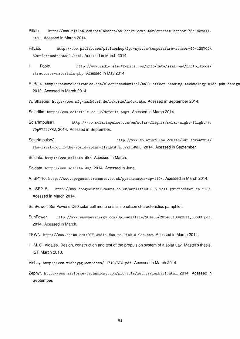
Pitlab. http://www.pitlab.com/pitlabshop/on-board-computer/current-sensor-75a-detail.
html. Acessed in March 2014.
PitLab. http://www.pitlab.com/pitlabshop/fpv-system/temperature-sensor-40-125%C2%
B0c-for-osd-detail.html. Acessed in March 2014.
I. Poole. http://www.radio-electronics.com/info/data/semicond/photo_diode/
structures-materials.php. Acessed in May 2014.
R. Racz. http://powerelectronics.com/electromechanical/hall-effect-sensing-technology-aids-pdu-design,
2012. Acessed in March 2014.
W. Shaeper. http://www.mfg-markdorf.de/rekorde/index.htm. Acessed in September 2014.
Solarfilm. http://www.solarfilm.co.uk/default.aspx. Acessed in March 2014.
SolarImpulse1. http://www.solarimpulse.com/en/solar-flights/solar-night-flight/#.
VDpVYfldWHW, 2014. Acessed in September.
SolarImpulse2. http://www.solarimpulse.com/en/our-adventure/
the-first-round-the-world-solar-flight#.VDpVZfldWHU, 2014. Acessed in September.
Soldata. http://www.soldata.dk/. Acessed in March.
Soldata. http://www.soldata.dk/, 2014. Acessed in June.
A. SP110. http://www.apogeeinstruments.co.uk/pyranometer-sp-110/. Acessed in March 2014.
A. SP215. http://www.apogeeinstruments.co.uk/amplified-0-5-volt-pyranometer-sp-215/.
Acessed in March 2014.
SunPower. SunPower’s C60 solar cell mono cristalline silicon characteristics pamphlet.
SunPower. http://www.easynewenergy.com/Uploads/file/201405/20140518042511_60693.pdf,
2014. Acessed in March.
TEWN. http://www.co-bw.com/DIY_Audio_How_to_Pick_a_Cap.htm. Acessed in March 2014.
H. M. G. Vidales. Design, construction and test of the propulsion system of a solar uav. Master’s thesis,
IST, March 2013.
Vishay. http://www.vishaypg.com/docs/11710/STC.pdf. Acessed in March 2014.
Zephyr. http://www.airforce-technology.com/projects/zephyr/zephyr1.html, 2014. Acessed in
September.
84

Appendix A
Equipment Technical Sheet
The technical sheets for most of the equipment used are shown here.
85
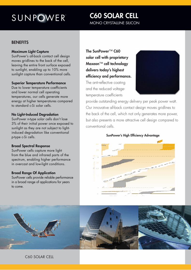
C60 SOLAR CELLMONO CRYSTALLINE SILICON
C60 SOLAR CELL
SunPower’s High Efficiency Advantage
BENEFITS
Maximum Light CaptureSunPower’s all-back contact cell design moves gridlines to the back of the cell, leaving the entire front surface exposed to sunlight, enabling up to 10% more sunlight capture than conventional cells.
Superior Temperature PerformanceDue to lower temperature coefficients and lower normal cell operating temperatures, our cells generate more energy at higher temperatures compared to standard c-Si solar cells.
No Light-Induced Degradation SunPower n-type solar cells don’t lose 3% of their initial power once exposed to sunlight as they are not subject to light-induced degradation like conventional p-type c-Si cells.
Broad Spectral Response SunPower cells capture more light from the blue and infrared parts of the spectrum, enabling higher performance in overcast and low-light conditions.
Broad Range Of ApplicationSunPower cells provide reliable performance in a broad range of applications for years to come.
The SunPower™ C60
solar cell with proprietary
Maxeon™ cell technology
delivers today’s highest
efficiency and performance.
The anti-reflective coating
and the reduced voltage-
temperature coefficients
provide outstanding energy delivery per peak power watt.
Our innovative all-back contact design moves gridlines to
the back of the cell, which not only generates more power,
but also presents a more attractive cell design compared to
conventional cells.
Photo courtesy of 3S Photovoltaics
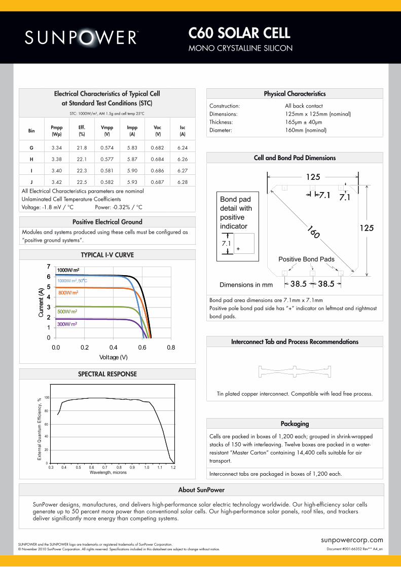
About SunPower
SunPower designs, manufactures, and delivers high-performance solar electric technology worldwide. Our high-efficiency solar cells generate up to 50 percent more power than conventional solar cells. Our high-performance solar panels, roof tiles, and trackers deliver significantly more energy than competing systems.
sunpowercorp.comSUNPOWER and the SUNPOWER logo are trademarks or registered trademarks of SunPower Corporation.
© November 2010 SunPower Corporation. All rights reserved. Specifications included in this datasheet are subject to change without notice. Document #001-66352 Rev** A4_en
Physical Characteristics
Construction:
Dimensions:
Thickness:
Diameter:
All back contact
125mm x 125mm (nominal)
165µm ± 40µm
160mm (nominal)
Packaging
Cells are packed in boxes of 1,200 each; grouped in shrink-wrapped
stacks of 150 with interleaving. Twelve boxes are packed in a water-
resistant “Master Carton” containing 14,400 cells suitable for air
transport.
Interconnect tabs are packaged in boxes of 1,200 each.
Cell and Bond Pad Dimensions
Bond pad area dimensions are 7.1mm x 7.1mm
Positive pole bond pad side has “+” indicator on leftmost and rightmost
bond pads.
Interconnect Tab and Process Recommendations
Tin plated copper interconnect. Compatible with lead free process.
C60 SOLAR CELLMONO CRYSTALLINE SILICON
TYPICAL I-V CURVE
Electrical Characteristics of Typical Cell
at Standard Test Conditions (STC)
STC: 1000W/m², AM 1.5g and cell temp 25°C
BinPmpp
(Wp)
Eff.
(%)
Vmpp
(V)
Impp
(A)
Voc
(V)
Isc
(A)
G 3.34 21.8 0.574 5.83 0.682 6.24
H 3.38 22.1 0.577 5.87 0.684 6.26
I 3.40 22.3 0.581 5.90 0.686 6.27
J 3.42 22.5 0.582 5.93 0.687 6.28
All Electrical Characteristics parameters are nominal
Unlaminated Cell Temperature Coefficients
Voltage: -1.8 mV / °C Power: -0.32% / °C
Positive Electrical Ground
Modules and systems produced using these cells must be configured as
“positive ground systems”.
SPECTRAL RESPONSE
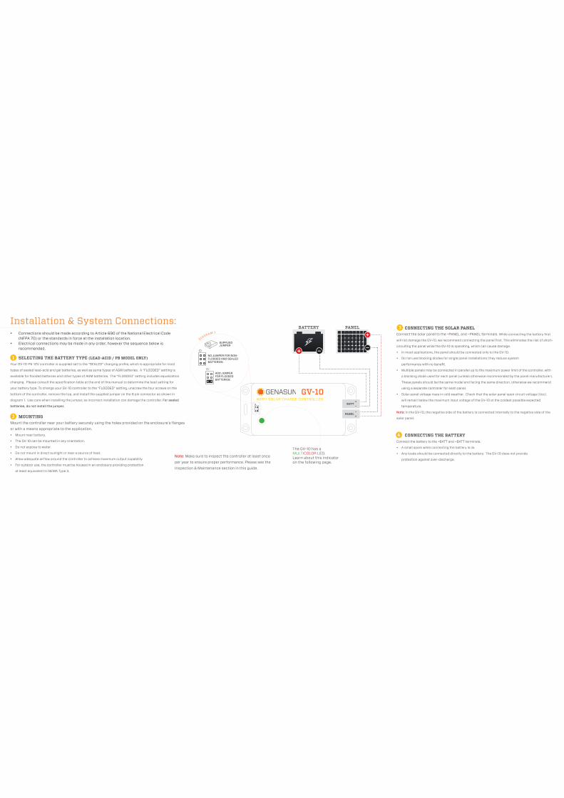
DIAGRAM 1
NO JUMPER FOR NON-FLOODED AND SEALED BATTERIES.
ADD JUMPER FOR FLOODED BATTERIES:
SUPPLIEDJUMPER
BATTERY PANELInstallation & System Connections:
MOUNTING
Mount the controller near your battery securely using the holes provided on the enclosure’s flanges
or with a means appropriate to the application.
• Mount near battery.
• The GV-10 can be mounted in any orientation.
• Do not expose to water.
• Do not mount in direct sunlight or near a source of heat.
• Allow adequate airflow around the controller to achieve maximum output capability.
• For outdoor use, the controller must be housed in an enclosure providing protection
at least equivalent to NEMA Type 3.
SELECTING THE BATTERY TYPE (LEAD-ACID / PB MODEL ONLY)
Your GV-10-Pb-12V controller is supplied set to the “SEALED” charging profile, which is appropriate for most
types of sealed lead-acid and gel batteries, as well as some types of AGM batteries. A “FLOODED” setting is
available for flooded batteries and other types of AGM batteries. The “FLOODED” setting includes equalization
charging. Please consult the specification table at the end of this manual to determine the best setting for
your battery type. To change your GV-10 controller to the “FLOODED” setting, unscrew the four screws on the
bottom of the controller, remove the top, and install the supplied jumper on the 6 pin connector as shown in
diagram 1. Use care when installing the jumper, as incorrect installation can damage the controller. For sealed
batteries, do not install the jumper.
r
e
CONNECTING THE SOLAR PANEL
Connect the solar panel to the +PANEL and –PANEL terminals. While connecting the battery first
will not damage the GV-10, we recommend connecting the panel first. This eliminates the risk of short-
circuiting the panel while the GV-10 is operating, which can cause damage.
• In most applications, the panel should be connected only to the GV-10.
• Do not use blocking diodes for single panel installations; they reduce system
performance with no benefit.
• Multiple panels may be connected in parallel up to the maximum power limit of the controller, with
a blocking diode used for each panel (unless otherwise recommended by the panel manufacturer).
These panels should be the same model and facing the same direction, otherwise we recommend
using a separate controller for each panel.
• Solar panel voltage rises in cold weather. Check that the solar panel open circuit voltage (Voc)
will remain below the maximum input voltage of the GV-10 at the coldest possible expected
temperature.
Note: In the GV-10, the negative side of the battery is connected internally to the negative side of the
solar panel.
• Connections should be made according to article 690 of the National electrical Code (NFPA 70) or the standards in force at the installation location.
• Electrical connections may be made in any order; however the sequence below is
recommended.
CONNECTING THE BATTERY
Connect the battery to the +BATT and –BATT terminals.
• A small spark while connecting the battery is ok.
• Any loads should be connected directly to the battery. The GV-10 does not provide
protection against over-discharge.
t
u
Note: Make sure to inspect the controller at least once
per year to ensure proper performance. Please see the
Inspection & Maintenance section in this guide.
The GV-10 has a MULTICOLOR LED.Learn about this indicator on the following page.
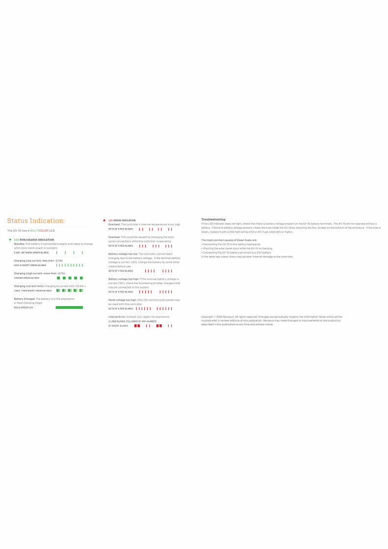
Troubleshooting
If the LED indicator does not light, check that there is battery voltage present on the GV-10 battery terminals. The GV-10 will not operate without a
battery. If there is battery voltage present, check the fuse inside the GV-10 by removing the four screws on the bottom of the enclosure. If the fuse is
blown, replace it with a 20A fast-acting ATO or ATC fuse rated 32V or higher.
The most common causes of blown fuses are:
• Connecting the gV-10 to the battery backwards• shorting the solar panel input while the gV-10 is charging• Connecting the gV-10 battery terminals to a 24V batteryIn the latter two cases, there may be other internal damage to the controller.
LED RUN/CHARGE INDICATION
Standby: The battery is connected properly and ready to charge
when solar panel power is available.
2 SEC. BETWEEN GREEN BLINKS
Charging (low current, less than ~3.7A):
FAST & SHORT GREEN BLINKS
Charging (high current, more than ~3.7A):
LONGER GREEN BLINKS
Charging (current limit): charging at current limit (10.5A+).
LONG, THEN SHORT GREEN BLINKS
Battery Charged: The battery is in the absorption
or float charging stage.
SOLID GREEN LED
LED ERROR INDICATION
Overheat: The controller’s internal temperature is too high.
SETS OF 2 RED BLINKS.
Overload: This could be caused by changing the solar
panel connections while the controller is operating.
SETS OF 3 RED BLINKS.
Battery voltage too low: The controller cannot begin
charging due to low battery voltage. If the nominal battery
voltage is correct (12V), charge the battery by some other
means before use.
SETS OF 4 RED BLINKS
Battery voltage too high: If the nominal battery voltage is
correct (12V), check the functioning of other chargers that
may be connected to the system.
SETS OF 5 RED BLINKS.
Panel voltage too high: Only 12V nominal solar panels may
be used with this controller.
SETS OF 6 RED BLINKS.
Internal Error: Contact your dealer for assistance.
2 LONG BLINKS, FOLLOWED BY ANY NUMBER
OF SHORT BLINKS.
The GV-10 has a MULTICOLOR LED
Status Indication:
Copyright © 2012 Genasun. All rights reserved. Changes are periodically made to the information herein which will be
incorporated in revised editions of this publication. Genasun may make changes or improvements to the product(s)
described in this publication at any time and without notice.
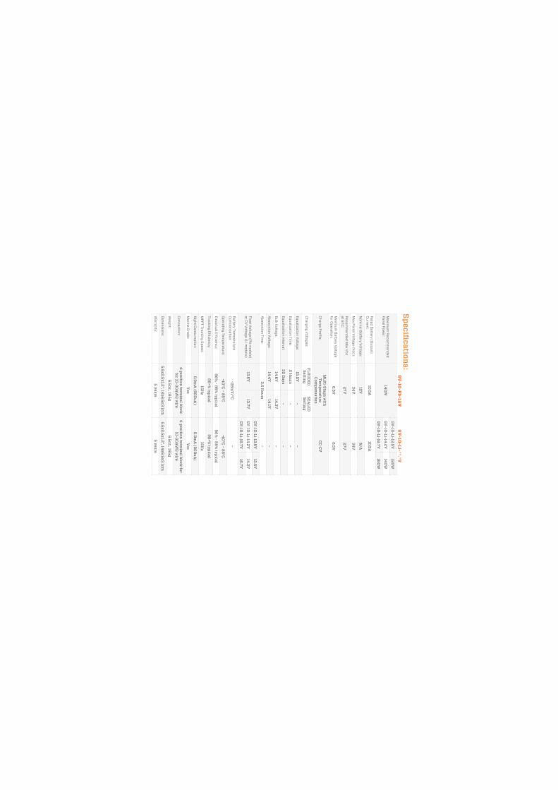
Sp
ec
ific
atio
ns
:
Ma
xim
um
Re
co
mm
en
de
d
Pa
ne
l Po
we
r:14
0W
GV
-10-L
i-12.5
V12
0W
GV
-10-L
i-14.2
V14
0W
GV
-10-L
i-16.7
V16
0W
Ra
ted
Ba
ttery
(Ou
tpu
t) C
urre
nt:
10.5
A10
.5A
No
min
al B
atte
ry V
olta
ge
:12
VN
/A
Ma
x P
an
el V
olta
ge
(Vo
c):
34
V3
4V
Re
co
mm
en
de
d M
ax
Vo
c
at S
TC
:2
7V
27
V
Min
imu
m B
atte
ry V
olta
ge
fo
r Op
era
tion
:8
.5V
8.5
V
Ch
arg
e P
rofile
:
Mu
lti-Sta
ge
with
T
em
pe
ratu
re
Co
mp
en
sa
tion
CC
-CV
Ch
arg
ing
Vo
ltag
es
:F
LO
OD
ED
S
ettin
gS
EA
LE
D
Se
tting
Eq
ua
liza
tion
Vo
ltag
e:
15.0
V–
–
Eq
ua
liza
tion
Tim
e:
2 H
ou
rs–
–
Eq
ua
liza
tion
Inte
rva
l:3
0 D
ay
s–
–
Bu
lk V
olta
ge
:14
.6V
14.3
V–
Ab
so
rptio
n V
olta
ge
:14
.4V
14.1V
–
Ab
so
rptio
n T
ime
:2
.5 H
ou
rs–
Flo
at V
olta
ge
(Pb
mo
de
ls)
or C
V V
olta
ge
(Li m
od
els
):13
.5V
13.7
V
GV
-10-L
i-12.5
V12
.5V
GV
-10-L
i-14.2
V14
.2V
GV
-10-L
i-16.7
V16
.7V
Ba
ttery
Te
mp
era
ture
C
om
pe
ns
atio
n:
-28
mV
/°C–
Op
era
ting
Te
mp
era
ture
:-4
0°C
– 8
5°C
-40
°C –
85
°C
Ele
ctric
al E
fficie
nc
y:
96
% - 9
8%
typ
ica
l9
6%
- 98
% ty
pic
al
Tra
ck
ing
Effic
ien
cy
:9
9+
% ty
pic
al
99
+%
typ
ica
l
MP
PT
Tra
ck
ing
Sp
ee
d:
15H
z15
Hz
Nig
ht C
on
su
mp
tion
:0
.9m
A (9
00
uA
)0
.9m
A (9
00
uA
)
Ma
rine
Gra
de
:Y
es
Ye
s
Co
nn
ec
tion
:4
-po
sitio
n te
rmin
al b
loc
k
for 10
-30
AW
G w
ire4
-po
sitio
n te
rmin
al b
loc
k fo
r 10
-30
AW
G w
ire
We
igh
t:6
.5o
z., 18
5g
6.5
oz
., 185
g
Dim
en
sio
ns
:5
.5x
2.5
x1.2
”, 14x
6.5
x3
.1cm
5.5
x2
.5x
1.2”, 14
x6
.5x
3.1c
m
Wa
rran
ty:
5 y
ea
rs5
ye
ars
GV-1
0-L
i-**.*V
GV-1
0-P
b-1
2V
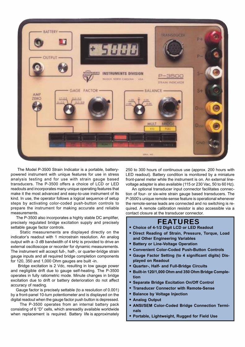
FEATURES
The Model P-3500 Strain Indicator is a portable, battery-
powered instrument with unique features for use in stress
analysis testing and for use with strain gauge based
transducers. The P-3500 offers a choice of LCD or LED
readouts and incorporates many unique operating features that
make it the most advanced and easy-to-use instrument of its
kind. In use, the operator follows a logical sequence of setup
steps by activating color-coded push-button controls to
prepare the instrument for making accurate and reliable
measurements.
The P-3500 also incorporates a highly stable DC amplifier,
precisely regulated bridge excitation supply and precisely
settable gauge factor controls.
Static measurements are displayed directly on the
indicator’s readout with 1 microstrain resolution. An analog
output with a -3 dB bandwidth of 4 kHz is provided to drive an
external oscilloscope or recorder for dynamic measurements.
The instrument will accept full-, half-, or quarter-bridge strain
gauge inputs and all required bridge completion components
for 120, 350 and 1,000 Ohm gauges are built -in.
Bridge excitation is 2 Vdc, resulting in low gauge power
and negligible drift due to gauge self-heating. The P-3500
operates in fully ratiometric mode. Minute changes in bridge
excitation due to drift or battery deterioration do not affect
accuracy of reading.
Gauge factor is precisely settable (to a resolution of 0.001)
by a front-panel 10-turn potentiometer and is displayed on the
digital readout when the gauge factor push button is depressed.
The P-3500 operates from an internal battery pack
consisting of 6 “D” cells, which arereadily available worldwide
when replacement is required. Battery life is approximately
250 to 300 hours of continuous use (approx. 200 hours with
LED readout). Battery condition is monitored by a miniature
front-panel meter while the instrument is on. An external line-
voltage adapter is also available (115 or 230 Vac, 50 to 60 Hz).
An optional transducer input connector facilitates connec-
tion of four- or six-wire strain gauge based transducers. The
P-3500’s unique remote-sense feature is operational whenever
the remote-sense leads are connected and no switching is re-
quired. A remote calibration resistor is also accessible via a
contact closure at the transducer connector.
••••• Choice of 4-1/2 Digit LCD or LED Readout
••••• Direct Reading of Strain, Pressure, Torque, Load
and Other Engineering Variables
••••• Battery or Line-Voltage Operation
••••• Convenient Color-Coded Push-Button Controls
••••• Gauge Factor Setting (to 4 significant digits) Dis-
played on Readout
••••• Quarter-, Half- and Full-Bridge Circuits
••••• Built-in 120/1,000 Ohm and 350 Ohm Bridge Comple-
tion
••••• Separate Bridge Excitation On/Off Control
••••• Transducer Connector with Remote-Sense
••••• Balance by Voltage Injection
••••• Analog Output
••••• ANSI/SEM Color-Coded Bridge Connection Termi-
nals
••••• Portable, Lightweight, Rugged for Field Use
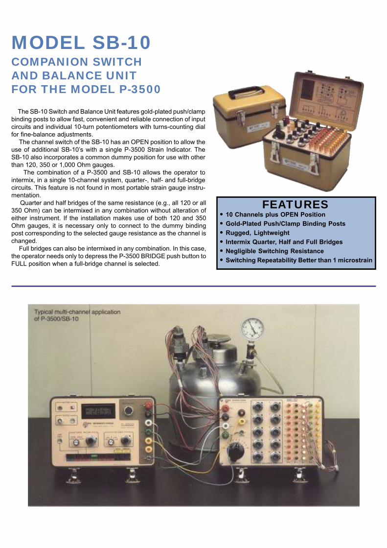
MODEL SB-10COMPANION SWITCHAND BALANCE UNITFOR THE MODEL P-3500
The SB-10 Switch and Balance Unit features gold-plated push/clamp
binding posts to allow fast, convenient and reliable connection of input
circuits and individual 10-turn potentiometers with turns-counting dial
for fine-balance adjustments.
The channel switch of the SB-10 has an OPEN position to allow the
use of additional SB-10’s with a single P-3500 Strain Indicator. The
SB-10 also incorporates a common dummy position for use with other
than 120, 350 or 1,000 Ohm gauges.
The combination of a P-3500 and SB-10 allows the operator to
intermix, in a single 10-channel system, quarter-, half- and full-bridge
circuits. This feature is not found in most portable strain gauge instru-
mentation.
Quarter and half bridges of the same resistance (e.g., all 120 or all
350 Ohm) can be intermixed in any combination without alteration of
either instrument. If the installation makes use of both 120 and 350
Ohm gauges, it is necessary only to connect to the dummy binding
post corresponding to the selected gauge resistance as the channel is
changed.
Full bridges can also be intermixed in any combination. In this case,
the operator needs only to depress the P-3500 BRIDGE push button to
FULL position when a full-bridge channel is selected.
FEATURES••••• 10 Channels plus OPEN Position
••••• Gold-Plated Push/Clamp Binding Posts
••••• Rugged, Lightweight
••••• Intermix Quarter, Half and Full Bridges
••••• Negligible Switching Resistance
••••• Switching Repeatability Better than 1 microstrain
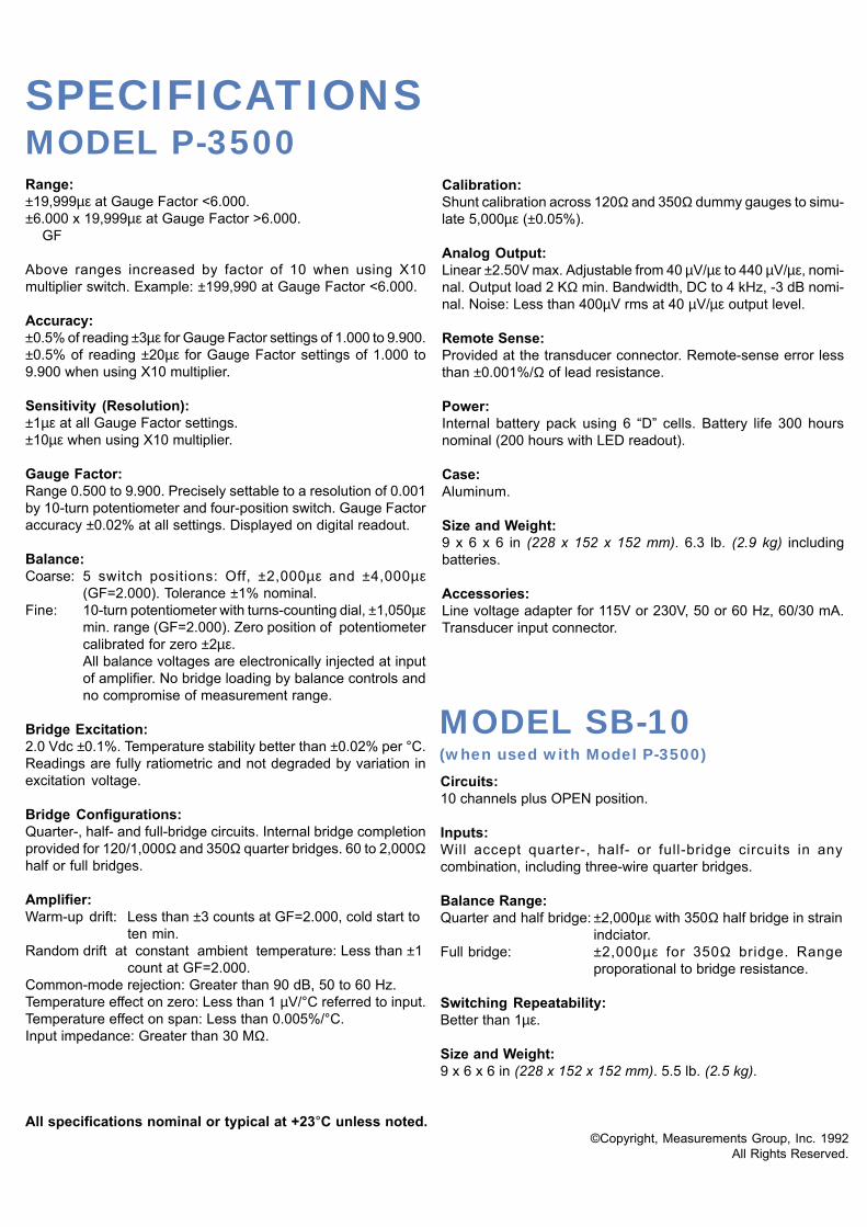
SPECIFICATIONSMODEL P-3500Range:
±19,999µε at Gauge Factor <6.000.
±6.000 x 19,999µε at Gauge Factor >6.000.
GF
Above ranges increased by factor of 10 when using X10
multiplier switch. Example: ±199,990 at Gauge Factor <6.000.
Accuracy:
±0.5% of reading ±3µε for Gauge Factor settings of 1.000 to 9.900.
±0.5% of reading ±20µε for Gauge Factor settings of 1.000 to
9.900 when using X10 multiplier.
Sensitivity (Resolution):
±1µε at all Gauge Factor settings.
±10µε when using X10 multiplier.
Gauge Factor:
Range 0.500 to 9.900. Precisely settable to a resolution of 0.001
by 10-turn potentiometer and four-position switch. Gauge Factor
accuracy ±0.02% at all settings. Displayed on digital readout.
Balance:
Coarse: 5 switch positions: Off, ±2,000µε and ±4,000µε(GF=2.000). Tolerance ±1% nominal.
Fine: 10-turn potentiometer with turns-counting dial, ±1,050µεmin. range (GF=2.000). Zero position of potentiometer
calibrated for zero ±2µε.
All balance voltages are electronically injected at input
of amplifier. No bridge loading by balance controls and
no compromise of measurement range.
Bridge Excitation:
2.0 Vdc ±0.1%. Temperature stability better than ±0.02% per °C.
Readings are fully ratiometric and not degraded by variation in
excitation voltage.
Bridge Configurations:
Quarter-, half- and full-bridge circuits. Internal bridge completion
provided for 120/1,000Ω and 350Ω quarter bridges. 60 to 2,000Ωhalf or full bridges.
Amplifier:
Warm-up drift: Less than ±3 counts at GF=2.000, cold start to
ten min.
Random drift at constant ambient temperature: Less than ±1
count at GF=2.000.
Common-mode rejection: Greater than 90 dB, 50 to 60 Hz.
Temperature effect on zero: Less than 1 µV/°C referred to input.
Temperature effect on span: Less than 0.005%/°C.
Input impedance: Greater than 30 MΩ.
Calibration:
Shunt calibration across 120Ω and 350Ω dummy gauges to simu-
late 5,000µε (±0.05%).
Analog Output:
Linear ±2.50V max. Adjustable from 40 µV/µε to 440 µV/µε, nomi-
nal. Output load 2 KΩ min. Bandwidth, DC to 4 kHz, -3 dB nomi-
nal. Noise: Less than 400µV rms at 40 µV/µε output level.
Remote Sense:
Provided at the transducer connector. Remote-sense error less
than ±0.001%/Ω of lead resistance.
Power:
Internal battery pack using 6 “D” cells. Battery life 300 hours
nominal (200 hours with LED readout).
Case:
Aluminum.
Size and Weight:
9 x 6 x 6 in (228 x 152 x 152 mm). 6.3 lb. (2.9 kg) including
batteries.
Accessories:
Line voltage adapter for 115V or 230V, 50 or 60 Hz, 60/30 mA.
Transducer input connector.
MODEL SB-10(w hen used w ith Model P-3500)
Circuits:
10 channels plus OPEN position.
Inputs:
Will accept quarter-, half- or full-bridge circuits in any
combination, including three-wire quarter bridges.
Balance Range:
Quarter and half bridge: ±2,000µε with 350Ω half bridge in strain
indciator.
Full bridge: ±2,000µε for 350Ω bridge. Range
proporational to bridge resistance.
Switching Repeatability:
Better than 1µε.
Size and Weight:
9 x 6 x 6 in (228 x 152 x 152 mm). 5.5 lb. (2.5 kg).
All specifications nominal or typical at +23°C unless noted.©Copyright, Measurements Group, Inc. 1992
All Rights Reserved.
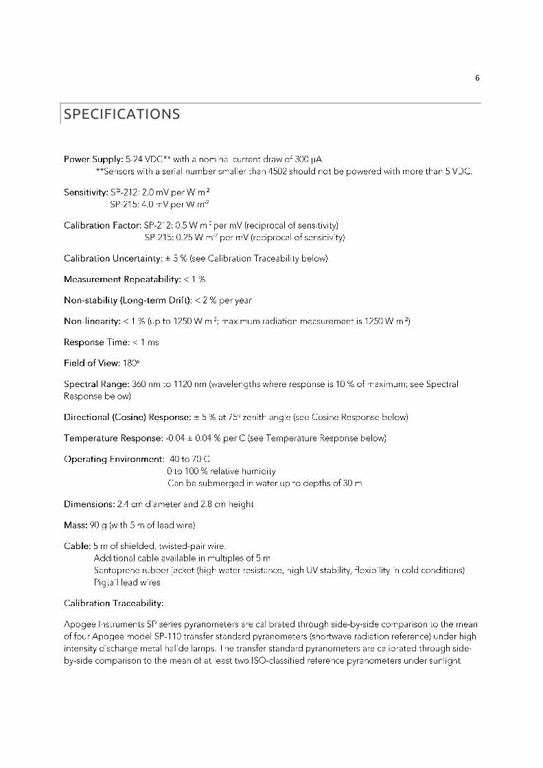
6
SPECIFICATIONS
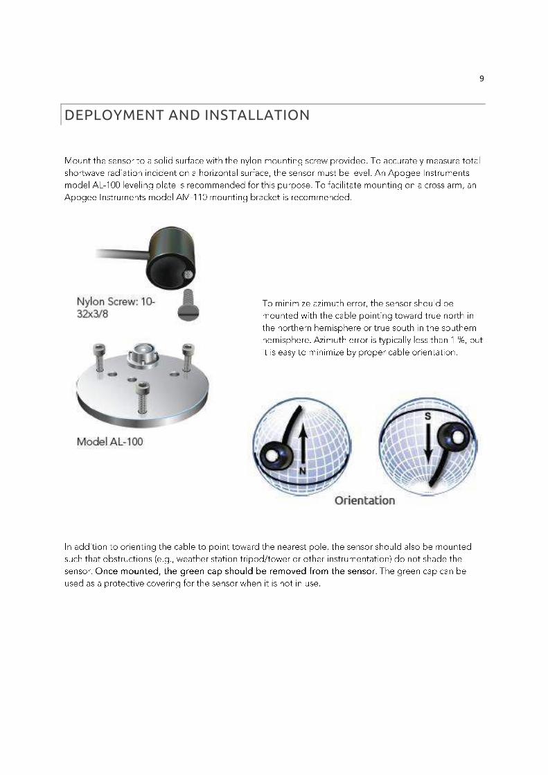
9
DEPLOYMENT AND INSTALLATION
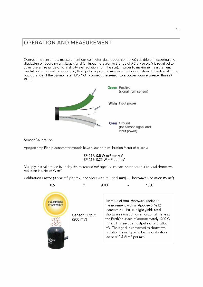
10
OPERATION AND MEASUREMENT