wing design optimization for a long-endurance uav using...

Copyright ⓒ The Korean Society for Aeronautical & Space SciencesReceived: December 28, 2015 Revised: June 7, 2016 Accepted: August 26, 2016

423 http://ijass.org pISSN: 2093-274x eISSN: 2093-2480

PaperInt’l J. of Aeronautical & Space Sci. 17(3), 423–431 (2016)DOI: http://dx.doi.org/10.5139/IJASS.2016.17.3.423

Wing Design Optimization for a Long-Endurance UAV using FSI Analysis and the Kriging Method

Seok-Ho Son*R&D Engineering Team, PIDO TECH Inc., Seoul 04763, Republic of Korea

Byung-Lyul Choi**Engineering Consulting Team, PIDO TECH Inc., Seoul 04763, Republic of Korea

Won-Jin Jin***Depart. of Aviation Maintenance Engineering, Far East University, Chungbuk 27601, Republic of Korea

Yung-Gyo Lee**** and Cheol-Wan Kim*****Aerodynamics Team, Korea Aerospace Research Inst., Dajeon 34133, Republic of Korea

Dong-Hoon Choi******School of Mechanical Engineering, Hanyang University, Seoul 04763, Republic of Korea

Abstract

In this study, wing design optimization for long-endurance unmanned aerial vehicles (UAVs) is investigated. The fluid-

structure integration (FSI) analysis is carried out to simulate the aeroelastic characteristics of a high-aspect ratio wing for a

long-endurance UAV. High-fidelity computational codes, FLUENT and DIAMOND/IPSAP, are employed for the loose coupling

FSI optimization. In addition, this optimization procedure is improved by adopting the design of experiment (DOE) and

Kriging model. A design optimization tool, PIAnO, integrates with an in-house codes, CAE simulation and an optimization

process for generating the wing geometry/computational mesh, transferring information, and finding the optimum solution.

The goal of this optimization is to find the best high-aspect ratio wing shape that generates minimum drag at a cruise condition

of CL = 1.0. The result shows that the optimal wing shape produced 5.95 % less drag compared to the initial wing shape.

Key words: Long endurance UAV(unmanned aerial vehicle), CFD(computational fluid dynamics), FSI(fluid-structure integration)

analysis, Design optimization, Kriging method

Nomenclature

α : Angle of attack

2

addition, this optimization procedure is improved by adopting the design of experiment (DOE) and

Kriging model. A design optimization tool, PIAnO, integrates with an in-house codes, CAE

simulation and an optimization process for generating the wing geometry/computational mesh,

transferring information, and finding the optimum solution. The goal of this optimization is to find the

best high-aspect ratio wing shape that generates minimum drag at a cruise condition of CL = 1.0. The

result shows that the optimal wing shape produced 5.95 % less drag compared to the initial wing

shape.

Key words: Long endurance UAV (unmanned aerial vehicle), CFD (computational fluid dynamics),

FSI (fluid-structure integration) analysis, Design optimization, Kriging method

Nomenclature

: Angle of attack

: Coefficient of regression

CL: Coefficient of drag

CD: Coefficient of lift

f x : Global model

: Dihedral angle

: Taper ratio

r : Correlation vector

R : Correlation function

R : Correlation matrix

V : Velocity (m/s)

x : Design variables

y x : Exact response model

y x : Approximated response model




2







shape.



Nomenclature

: Angle of attack




f x : Global model

: Dihedral angle

: Taper ratio




V : Velocity (m/s)




: Global model

Γ : Dihedral angle

λ : Taper ratio

2







shape.



Nomenclature

: Angle of attack




f x : Global model

: Dihedral angle

: Taper ratio




V : Velocity (m/s)




: Correlation vector


2







shape.



Nomenclature

: Angle of attack




f x : Global model

: Dihedral angle

: Taper ratio




V : Velocity (m/s)




: Correlation matrix

V : Velocity (m/s)

2







shape.



Nomenclature

: Angle of attack




f x : Global model

: Dihedral angle

: Taper ratio




V : Velocity (m/s)




: Design variables

This is an Open Access article distributed under the terms of the Creative Com-mons Attribution Non-Commercial License (http://creativecommons.org/licenses/by-nc/3.0/) which permits unrestricted non-commercial use, distribution, and reproduc-tion in any medium, provided the original work is properly cited.

* Ph. D ** Ph. D *** Professor **** Ph. D ***** Ph. D ****** Professor, Corresponding author: [email protected]

DOI: http://dx.doi.org/10.5139/IJASS.2016.17.3.423 424

Int’l J. of Aeronautical & Space Sci. 17(3), 423–431 (2016)

2







shape.



Nomenclature

: Angle of attack




f x : Global model

: Dihedral angle

: Taper ratio




V : Velocity (m/s)




: Exact response model

2







shape.



Nomenclature

: Angle of attack




f x : Global model

: Dihedral angle

: Taper ratio




V : Velocity (m/s)



y x : Approximated response model : Approximated response model

3

Z x : Local deviation model

1. Introduction

The importance of long-endurance unmanned aerial vehicles (UAVs) in future airfields will be

growing due to their versatility in many applications, such as executing strategic reconnaissance,

providing telecommunication links, and helping in metrological research, forest fire detection, and

disaster monitoring. Therefore, design optimization techniques for long-endurance UAVs have been

investigated to improve their flight performance and to reduce the development effort. Rajagopal et al.

[1-2] proposed a multi-disciplinary design optimization (MDO) for optimizing the conceptual design

of a long-endurance UAV with the panel method code, XFLR5. Park et al. [3] employed a simple

multi-objective genetic algorithm to find an optimum airfoil shape for a long-endurance UAV.

High-aspect ratio wings of a long-endurance UAV are needed to minimize the induced drag and

easily cause wing deflection and deformation during flight [4, 5]. This tendency during flight can

cause incorrect prediction results if aerodynamic analysis is performed assuming a rigid wing.

Therefore, fluid -structure integration (FSI) analysis must be used in wing design optimization in

order to simulate a more accurate and realistic interaction between the aerodynamic loads and the

structural components of the aircraft wing.

FSI has two approaches: close coupling and loose coupling [6]. The close coupling approach

requires large computational resources since it reformulates and resolves the numerical equations by

combining the fluid and structural motion simultaneously. The second approach, loose coupling, deals

with only external interactions between the aerodynamic and structural models. Therefore, many

researchers have applied the loose coupling FSI to optimize an UAV wing design. For instance,

Gonzalez et al. applied loose coupling multi-physics to a long-endurance UAV wing design using

XFOIL/ MSES/ NSC2ke and NASTRAN for aerodynamic and structural analyses, respectively [7].

The meta-model techniques, such as the Kriging model, support vector regression (SVR) and

artificial neural network (ANN), contribute to simplifying the wing design optimization procedure and

produce optimum results without a large amount of expensive simulation. Consequently, the meta-

: Local deviation model

1. Introduction

The importance of long-endurance unmanned aerial

vehicles (UAVs) in future airfields will be growing due to their

versatility in many applications, such as executing strategic

reconnaissance, providing telecommunication links, and

helping in metrological research, forest fire detection,

and disaster monitoring. Therefore, design optimization

techniques for long-endurance UAVs have been investigated

to improve their flight performance and to reduce the

development effort. Rajagopal et al. [1-2] proposed a multi-

disciplinary design optimization (MDO) for optimizing the

conceptual design of a long-endurance UAV with the panel

method code, XFLR5. Park et al. [3] employed a simple

multi-objective genetic algorithm to find an optimum airfoil

shape for a long-endurance UAV.

High-aspect ratio wings of a long-endurance UAV are

needed to minimize the induced drag and easily cause

wing deflection and deformation during flight [4, 5]. This

tendency during flight can cause incorrect prediction results

if aerodynamic analysis is performed assuming a rigid wing.

Therefore, fluid -structure integration (FSI) analysis must be

used in wing design optimization in order to simulate a more

accurate and realistic interaction between the aerodynamic

loads and the structural components of the aircraft wing.

FSI has two approaches: close coupling and loose

coupling [6]. The close coupling approach requires large

computational resources since it reformulates and resolves

the numerical equations by combining the fluid and

structural motion simultaneously. The second approach,

loose coupling, deals with only external interactions between

the aerodynamic and structural models. Therefore, many

researchers have applied the loose coupling FSI to optimize

an UAV wing design. For instance, Gonzalez et al. applied

loose coupling multi-physics to a long-endurance UAV wing

design using XFOIL/ MSES/ NSC2ke and NASTRAN for

aerodynamic and structural analyses, respectively [7].

The meta-model techniques, such as the Kriging

model, support vector regression (SVR) and artificial

neural network (ANN), contribute to simplifying the wing

design optimization procedure and produce optimum

results without a large amount of expensive simulation.

Consequently, the meta-model techniques like SVR and

ANN have been incorporated into the UAV aircraft design,

especially in the design of their wing components.

Lee et al. suggested the design optimization of a long-

endurance UAV wing by using loose coupling FSI analysis

and the ANN technique [8]. Lam et al. studied an integrated

multi-objective optimization algorithm based on the Kriging

method to investigate aerodynamically or structurally

optimized transonic wings [9].

In this study, we optimized the design procedure using

FSI analysis and the Kriging method. The goal of this

study is finding the optimized shape of a high-aspect ratio

wing planform having minimum drag for an electrically

powered long-endurance UAV. Loose coupling FSI analysis

is performed with high-fidelity computational aerodynamic

and structural analysis codes, FLUENT and DIAMOND/

IPSAP. These analyses simulate realistic aeroelastic behaviors

of the long endurance UAV wing. We especially introduce

the design guidelines in which design variables influence

the system response of UAV. In addition, we suggest that

how to find the optimum solution efficiently though the

optimization techniques: design of experiment (DOE) and

Kriging method. Finally, we propose the optimum solution

to improve the efficiency and accuracy of the long endurance

UAV.

2. Optimization Procedure

2.1 FSI analysis

The wing shape of a flying airplane experiences

deformations due to the wing’s aerodynamic load (the wing

is the main source of lift force). The aeroelastic deformation of

aircraft wings are usually presented by an upward deflection

and a twist motion. Therefore, aerodynamic analysis based

on rigid wing shapes could lead to incorrect results.

To avoid these, we use an FSI analysis that considers

the coupling effects of an aerodynamic load as well as

structural deformation. The computation results of an

external aerodynamic load are distributed on the wing

surface. Structural analysis of the designed component

layouts and material properties of external and internal

wing structures is carried out to calculate the amount and

direction of deformation caused by the aerodynamic effect.

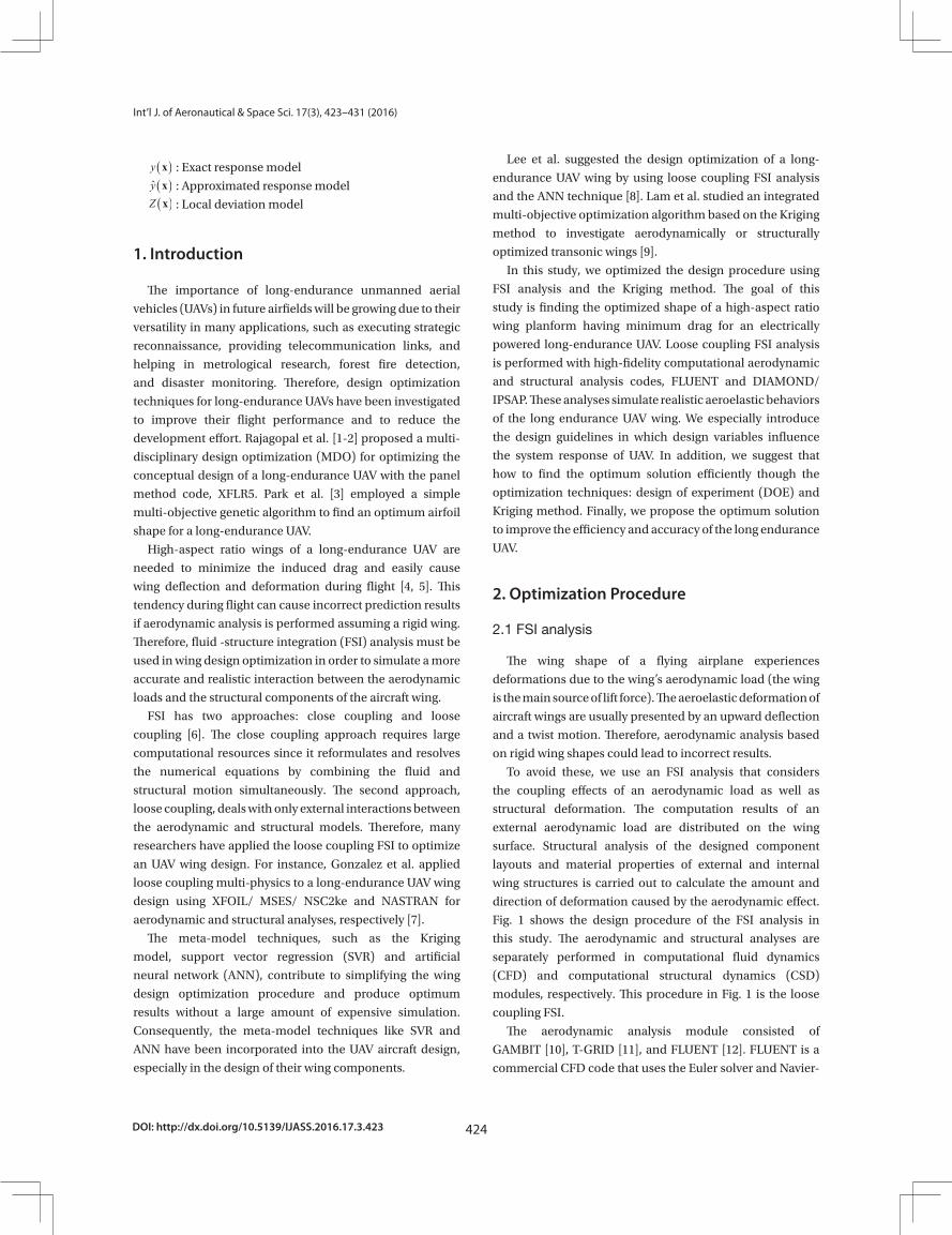
Fig. 1 shows the design procedure of the FSI analysis in

this study. The aerodynamic and structural analyses are

separately performed in computational fluid dynamics

(CFD) and computational structural dynamics (CSD)

modules, respectively. This procedure in Fig. 1 is the loose

coupling FSI.

The aerodynamic analysis module consisted of

GAMBIT [10], T-GRID [11], and FLUENT [12]. FLUENT is a

commercial CFD code that uses the Euler solver and Navier-

425

Seok-Ho Son Wing Design Optimization for a Long-Endurance UAV using FSI Analysis and the Kriging Method

http://ijass.org

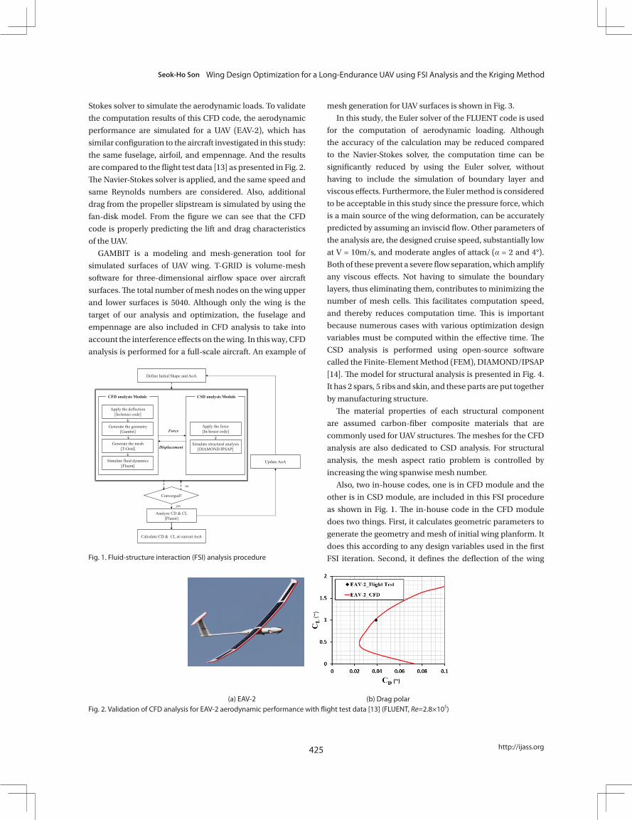
Stokes solver to simulate the aerodynamic loads. To validate

the computation results of this CFD code, the aerodynamic

performance are simulated for a UAV (EAV-2), which has

similar configuration to the aircraft investigated in this study:

the same fuselage, airfoil, and empennage. And the results

are compared to the flight test data [13] as presented in Fig. 2.

The Navier-Stokes solver is applied, and the same speed and

same Reynolds numbers are considered. Also, additional

drag from the propeller slipstream is simulated by using the

fan-disk model. From the figure we can see that the CFD

code is properly predicting the lift and drag characteristics

of the UAV.

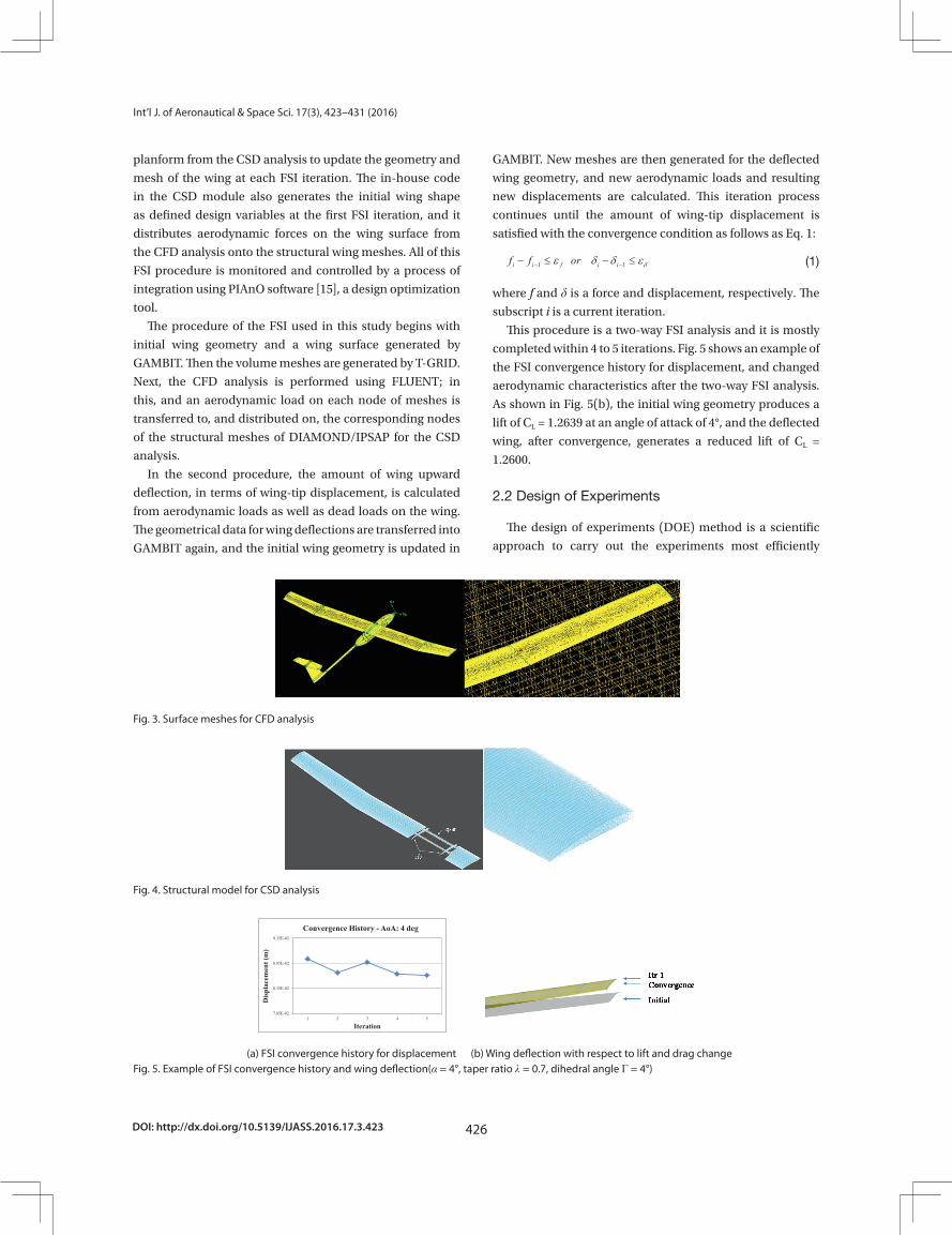
GAMBIT is a modeling and mesh-generation tool for

simulated surfaces of UAV wing. T-GRID is volume-mesh

software for three-dimensional airflow space over aircraft

surfaces. The total number of mesh nodes on the wing upper

and lower surfaces is 5040. Although only the wing is the

target of our analysis and optimization, the fuselage and

empennage are also included in CFD analysis to take into

account the interference effects on the wing. In this way, CFD

analysis is performed for a full-scale aircraft. An example of

mesh generation for UAV surfaces is shown in Fig. 3.

In this study, the Euler solver of the FLUENT code is used

for the computation of aerodynamic loading. Although

the accuracy of the calculation may be reduced compared

to the Navier-Stokes solver, the computation time can be

significantly reduced by using the Euler solver, without

having to include the simulation of boundary layer and

viscous effects. Furthermore, the Euler method is considered

to be acceptable in this study since the pressure force, which

is a main source of the wing deformation, can be accurately

predicted by assuming an inviscid flow. Other parameters of

the analysis are, the designed cruise speed, substantially low

at V = 10m/s, and moderate angles of attack (α = 2 and 4°).

Both of these prevent a severe flow separation, which amplify

any viscous effects. Not having to simulate the boundary

layers, thus eliminating them, contributes to minimizing the

number of mesh cells. This facilitates computation speed,

and thereby reduces computation time. This is important

because numerous cases with various optimization design

variables must be computed within the effective time. The

CSD analysis is performed using open-source software

called the Finite-Element Method (FEM), DIAMOND/IPSAP

[14]. The model for structural analysis is presented in Fig. 4.

It has 2 spars, 5 ribs and skin, and these parts are put together

by manufacturing structure.

The material properties of each structural component

are assumed carbon-fiber composite materials that are

commonly used for UAV structures. The meshes for the CFD

analysis are also dedicated to CSD analysis. For structural

analysis, the mesh aspect ratio problem is controlled by

increasing the wing spanwise mesh number.

Also, two in-house codes, one is in CFD module and the

other is in CSD module, are included in this FSI procedure

as shown in Fig. 1. The in-house code in the CFD module

does two things. First, it calculates geometric parameters to

generate the geometry and mesh of initial wing planform. It

does this according to any design variables used in the first

FSI iteration. Second, it defines the deflection of the wing

21

Fig. 1. Fluid-structure interaction (FSI) analysis procedure

Define Initial Shape and AoA

Generate the geometry[Gambit]

Converged?

Analyze CD & CL [Fluent]

Calculate CD & CL at current AoA

Force

yes

no

Update AoA

Generate the mesh[T-Grid]

Simulate fluid dynamics[Fluent]

Displacement

Apply the force[In-house code]

Apply the deflection[In-house code]

Simulate structural analysis[DIAMOND/IPSAP]

CFD analysis Module CSD analysis Module

Fig. 1. Fluid-structure interaction (FSI) analysis procedure

22

(a) EAV-2 (b) Drag polar

Fig. 2. Validation of CFD analysis for EAV-2 aerodynamic performance with flight test data [13]

(FLUENT, Re=2.8×105)

(a) EAV-2 (b) Drag polarFig. 2. Validation of CFD analysis for EAV-2 aerodynamic performance with flight test data [13] (FLUENT, Re=2.8×105)



planform from the CSD analysis to update the geometry and

mesh of the wing at each FSI iteration. The in-house code

in the CSD module also generates the initial wing shape

as defined design variables at the first FSI iteration, and it

distributes aerodynamic forces on the wing surface from

the CFD analysis onto the structural wing meshes. All of this

FSI procedure is monitored and controlled by a process of

integration using PIAnO software [15], a design optimization

tool.

The procedure of the FSI used in this study begins with

initial wing geometry and a wing surface generated by

GAMBIT. Then the volume meshes are generated by T-GRID.

Next, the CFD analysis is performed using FLUENT; in

this, and an aerodynamic load on each node of meshes is

transferred to, and distributed on, the corresponding nodes

of the structural meshes of DIAMOND/IPSAP for the CSD

analysis.

In the second procedure, the amount of wing upward

deflection, in terms of wing-tip displacement, is calculated

from aerodynamic loads as well as dead loads on the wing.

The geometrical data for wing deflections are transferred into

GAMBIT again, and the initial wing geometry is updated in

GAMBIT. New meshes are then generated for the deflected

wing geometry, and new aerodynamic loads and resulting

new displacements are calculated. This iteration process

continues until the amount of wing-tip displacement is

satisfied with the convergence condition as follows as Eq. 1:

7

GAMBIT. New meshes are then generated for the deflected wing geometry, and new aerodynamic

loads and resulting new displacements are calculated. This iteration process continues until the

amount of wing-tip displacement is satisfied with the convergence condition as follows as Eq. 1:

1 1i i f i if f or (1)

where f and is a force and displacement, respectively. The subscript i is a current iteration.

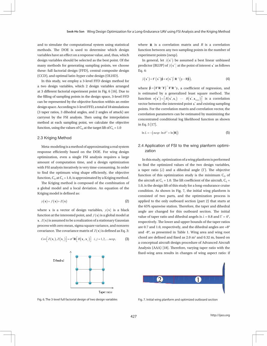
This procedure is a two-way FSI analysis and it is mostly completed within 4 to 5 iterations. Fig. 5

shows an example of the FSI convergence history for displacement, and changed aerodynamic

characteristics after the two-way FSI analysis. As shown in Fig. 5(b), the initial wing geometry

produces a lift of CL = 1.2639 at an angle of attack of 4°, and the deflected wing, after convergence,

generates a reduced lift of CL = 1.2600.

2.2 Design of Experiments

The design of experiments (DOE) method is a scientific approach to carry out the experiments most

efficiently and to simulate the computational system using statistical methods. The DOE is used to

determine which design variables have an effect on a response value, and, thus, which design

variables should be selected as the best point. Of the many methods for generating sampling points,

we choose these: full factorial design (FFD), central composite design (CCD), and optimal latin-hyper

cube design (OLHD).

In this study, we employ a 3-level FFD design method for a two design variables, which 2 design

variables arranged at 3 different factorial experiment point in Fig. 6 [16]. Due to the filling of

sampling points in the design space, 3-level FFD can be represented by the objective function within

an entire design space. According to 3-level FFD, a total of 18 simulations (3 taper ratios, 3 dihedral

angles, and 2 angles of attack) are carryout by the FSI analysis. Then using the interpolation method

at each sampling point, we calculate the objective function, using the values of CD at the target lift of

CL = 1.0

(1)

where f and δ is a force and displacement, respectively. The

subscript i is a current iteration.

This procedure is a two-way FSI analysis and it is mostly

completed within 4 to 5 iterations. Fig. 5 shows an example of

the FSI convergence history for displacement, and changed

aerodynamic characteristics after the two-way FSI analysis.

As shown in Fig. 5(b), the initial wing geometry produces a

lift of CL = 1.2639 at an angle of attack of 4°, and the deflected

wing, after convergence, generates a reduced lift of CL =

1.2600.

2.2 Design of Experiments

The design of experiments (DOE) method is a scientific

approach to carry out the experiments most efficiently

23

Fig. 3. Surface meshes for CFD analysis

Fig. 3. Surface meshes for CFD analysis

24

Fig. 4. Structural model for CSD analysis

Fig. 4. Structural model for CSD analysis

25

(a) FSI convergence history for displacement (b) Wing deflection with respect to lift and drag change

Fig. 5. Example of FSI convergence history and wing deflection ( = 4°, taper ratio = 0.7, dihedral angle = 4°)

7.85E-02

8.35E-02

8.85E-02

9.35E-02

1 2 3 4 5

Disp

lace

men

t (m

)

Iteration

Convergence History - AoA: 4 deg

(a) FSI convergence history for displacement (b) Wing deflection with respect to lift and drag changeFig. 5. Example of FSI convergence history and wing deflection(α = 4°, taper ratio λ = 0.7, dihedral angle Γ = 4°)

427


http://ijass.org

and to simulate the computational system using statistical

methods. The DOE is used to determine which design

variables have an effect on a response value, and, thus, which

design variables should be selected as the best point. Of the

many methods for generating sampling points, we choose

these: full factorial design (FFD), central composite design

(CCD), and optimal latin-hyper cube design (OLHD).

In this study, we employ a 3-level FFD design method for

a two design variables, which 2 design variables arranged

at 3 different factorial experiment point in Fig. 6 [16]. Due to

the filling of sampling points in the design space, 3-level FFD

can be represented by the objective function within an entire

design space. According to 3-level FFD, a total of 18 simulations

(3 taper ratios, 3 dihedral angles, and 2 angles of attack) are

carryout by the FSI analysis. Then using the interpolation

method at each sampling point, we calculate the objective

function, using the values of CD at the target lift of CL = 1.0

2.3 Kriging Method

Meta-modeling is a method of approximating a real system

response efficiently based on the DOE. For wing design

optimization, even a single FSI analysis requires a large

amount of computation time, and a design optimization

with FSI analysis iteratively is very time-consuming. In order

to find the optimum wing shape efficiently, the objective

function, CD at CL = 1.0, is approximated by a Kriging method.

The Kriging method is composed of the combination of

a global model and a local deviation. An equation of the

Kriging model is defined as:

8

2.3 Kriging Method

Meta-modeling is a method of approximating a real system response efficiently based on the DOE.

For wing design optimization, even a single FSI analysis requires a large amount of computation time,

and a design optimization with FSI analysis iteratively is very time-consuming. In order to find the

optimum wing shape efficiently, the objective function, CD at CL = 1.0, is approximated by a Kriging

method.

The Kriging method is composed of the combination of a global model and a local deviation. An

equation of the Kriging model is defined as:

y f Z x x x (2)

where x is a vector of design variables, y x is a black function at the interested point, and f x is

a global model at x . Z x is assumed to be a realization of a stationary Gaussian process with zero

mean, sigma square variance, and nonzero covariance. The covariance matrix of Z x is defined as

Eq. 3:

2, , , 1, 2, ,i j i jCov Z Z R i j nexp x x R x x (3)

where R is a correlation matrix and R is a correlation function between any two sampling points in

the number of experiment points (nexp).

In general, let *y x be assumed a best linear unbiased predictor (BLUP) of *y x at the point of

interest *x as follows Eq. 4:

* * * 1ˆ ˆˆ ,tty x f x β r x R y Fβ (4)

(2)

where

8

2.3 Kriging Method





method.



y f Z x x x (2)




Eq. 3:







is a vector of design variables,

8

2.3 Kriging Method





method.



y f Z x x x (2)




Eq. 3:







is a black

function at the interested point, and

8

2.3 Kriging Method





method.



y f Z x x x (2)




Eq. 3:







is a global model at

8

2.3 Kriging Method





method.



y f Z x x x (2)




Eq. 3:







.

8

2.3 Kriging Method





method.



y f Z x x x (2)




Eq. 3:







is assumed to be a realization of a stationary Gaussian

process with zero mean, sigma square variance, and nonzero

covariance. The covariance matrix of

8

2.3 Kriging Method





method.



y f Z x x x (2)




Eq. 3:







is defined as Eq. 3:

8

2.3 Kriging Method





method.



y f Z x x x (2)




Eq. 3:







(3)

where

8

2.3 Kriging Method





method.



y f Z x x x (2)




Eq. 3:







is a correlation matrix and R is a correlation

function between any two sampling points in the number of

experiment points (nexp).

In general, let

8

2.3 Kriging Method





method.



y f Z x x x (2)




Eq. 3:







be assumed a best linear unbiased

predictor (BLUP) of

8

2.3 Kriging Method





method.



y f Z x x x (2)




Eq. 3:







at the point of interest

8

2.3 Kriging Method





method.



y f Z x x x (2)




Eq. 3:







as follows

Eq. 4:

8

2.3 Kriging Method





method.



y f Z x x x (2)




Eq. 3:






* * * 1ˆ ˆˆ ,tty x f x β r x R y Fβ (4) (4)

where

9

where 11 1ˆ t t β F R F F R y , a coefficient of regression, and is estimated by a generalized least square

method. The function * * *1, ,

t

nexpR R r x x x x x is a correlation vector between the

interested point *x and existing sampling points. For the correlation matrix and correlation vector, the

correlation parameters can be estimated by maximizing the concentrated conditional log likelihood

function as shown in Eq. 5 [17].

2ˆln ln lnL nexp R (5)

2.4 Application of FSI to the wing planform optimization

In this study, optimization of a wing planform is performed to find the optimized values of the two

design variables, a taper ratio ( ) and a dihedral angle ( ). The objective function of this

optimization study is the minimum CD of the aircraft at CL = 1.0. The lift coefficient of the aircraft, CL

= 1.0, is the design lift of this study for a long-endurance cruise condition. As shown in Fig. 7, the

initial wing planform is consisted of two parts, and the optimization process is applied to the only

outboard section (part 2) that starts at the 65% spanwise station. Therefore, the taper and dihedral

angle are changed for this outboard section. The initial value of taper ratio and dihedral angels is λ =

0.8 and Γ = 4°, respectively. The lower and upper bounds of the taper ratios are 0.7 and 1.0,

respectively, and the dihedral angles are +8° and -8°, as presented in Table 1. Wing area and wing root

chord are defined and fixed as 2.0 m2 and 0.32 m, based on a conceptual aircraft design procedure of

Advanced Aircraft Analysis (AAA) [18]. Therefore, varying taper ratio with the fixed-wing area

results in changes of wing aspect ratio: if the taper ratio decreases, wing aspect ratio increases. In

general, higher aspect ratio (lower taper ratio) wing requires structural reinforcement. Therefore, the

taper ratio below λ = 0.7 is not considered since a lower-taper ratio increases the structural weight of a

wing. The λ = 0.8 is corresponding to AR=20, which is already a high aspect ratio in the practical

wing structural design. The design limits for the dihedral angles (8° ≤ Γ ≤ 8°) are defined due to the

, a coefficient of regression, and

is estimated by a generalized least square method. The

function

9



t























is a correlation

vector between the interested point

8

2.3 Kriging Method





method.



y f Z x x x (2)




Eq. 3:







and existing sampling

points. For the correlation matrix and correlation vector, the

correlation parameters can be estimated by maximizing the

concentrated conditional log likelihood function as shown

in Eq. 5 [17].

9



t























(5)

2.4 Application of FSI to the wing planform optimi-zation

In this study, optimization of a wing planform is performed

to find the optimized values of the two design variables,

a taper ratio (λ) and a dihedral angle (Γ). The objective

function of this optimization study is the minimum CD of

the aircraft at CL = 1.0. The lift coefficient of the aircraft, CL =

1.0, is the design lift of this study for a long-endurance cruise

condition. As shown in Fig. 7, the initial wing planform is

consisted of two parts, and the optimization process is

applied to the only outboard section (part 2) that starts at

the 65% spanwise station. Therefore, the taper and dihedral

angle are changed for this outboard section. The initial

value of taper ratio and dihedral angels is λ = 0.8 and Γ = 4°,

respectively. The lower and upper bounds of the taper ratios

are 0.7 and 1.0, respectively, and the dihedral angles are +8°

and -8°, as presented in Table 1. Wing area and wing root

chord are defined and fixed as 2.0 m2 and 0.32 m, based on

a conceptual aircraft design procedure of Advanced Aircraft

Analysis (AAA) [18]. Therefore, varying taper ratio with the

fixed-wing area results in changes of wing aspect ratio: if

26

Fig. 6. The 3-level full factorial design of two design variables

Fig. 6. The 3-level full factorial design of two design variables

27

Fig. 7. Initial wing planform and optimized outboard section

Fig. 7. Initial wing planform and optimized outboard section



the taper ratio decreases, wing aspect ratio increases. In

general, higher aspect ratio (lower taper ratio) wing requires

structural reinforcement. Therefore, the taper ratio below λ =

0.7 is not considered since a lower-taper ratio increases the

structural weight of a wing. The λ = 0.8 is corresponding to

AR=20, which is already a high aspect ratio in the practical

wing structural design. The design limits for the dihedral

angles (8° ≤ Γ ≤ 8°) are defined due to the similar reason. Also

note that even though the dihedral angle controls the lateral

stability of aircraft, it is only considered as a design variable

to optimize such that it could affect the wing’s aerodynamic

performance coupled with the effect of wing deflection.

Two angles of attack, α = 2 and 4°, are considered, and

this angle range covers the expected cruise angle of attack.

As mentioned above, the optimization problem of this study

is that the objective function (a minimum drag, CD) with

constant lift (CL = 1.0) is obtained by the taper ratio (λ) and

the dihedral angle (Γ). We try to optimize the taper ratio and

dihedral angle so that they minimize CD at CL = 1.0 as follows

in Eq. 6.

10

similar reason. Also note that even though the dihedral angle controls the lateral stability of aircraft, it

is only considered as a design variable to optimize such that it could affect the wing’s aerodynamic


Two angles of attack, α = 2 and 4°, are considered, and this angle range covers the expected cruise

angle of attack. As mentioned above, the optimization problem of this study is that the objective

function (a minimum drag, CD) with constant lift (CL = 1.0) is obtained by the taper ratio ( ) and the

dihedral angle ( ). We try to optimize the taper ratio and dihedral angle so that they minimize CD at

CL = 1.0 as follows in Eq. 5.

,

@ 1.0D L

FindMinimize C C

(5)

The optimization process based on FSI analysis requires a large amount of time and computational

resource because the FSI analysis must be simulated at every iteration of a new case. To improve the

procedure efficiency, we optimize by carrying out DOE and the Kriging method. An approximate

optimization problem is defined as follows Eq. 6:

,

ˆ ˆ@ 1.0D L

Find

Minimize C C

, (6)

where ˆ ˆ,D LC C is an approximated coefficients of drag and lift, both calculated by the Kriging model.

The optimization algorithms we use with DOE, Kriging method and global optimizer, are also

automatically executed by using the PIAnO software.

3. Results and discussion

3.1 FSI analysis results

The FSI analysis results for 18 DOE cases are tabulated in Table 2. These cases are differentiated

from each other by three different taper ratios, three different dihedral angles, and two angles of attack.

(6)

The optimization process based on FSI analysis requires

a large amount of time and computational resource because

the FSI analysis must be simulated at every iteration of a new

case. To improve the procedure efficiency, we optimize by

carrying out DOE and the Kriging method. An approximate


10









,

@ 1.0D L

FindMinimize C C

(5)





,

ˆ ˆ@ 1.0D L

Find

Minimize C C

, (6)








(7)

where

10









,

@ 1.0D L

FindMinimize C C

(5)





,

ˆ ˆ@ 1.0D L

Find

Minimize C C

, (6)








is an approximated coefficients of drag and lift,

both calculated by the Kriging model.

The optimization algorithms we use with DOE, Kriging

method and global optimizer, are also automatically

executed by using the PIAnO software.



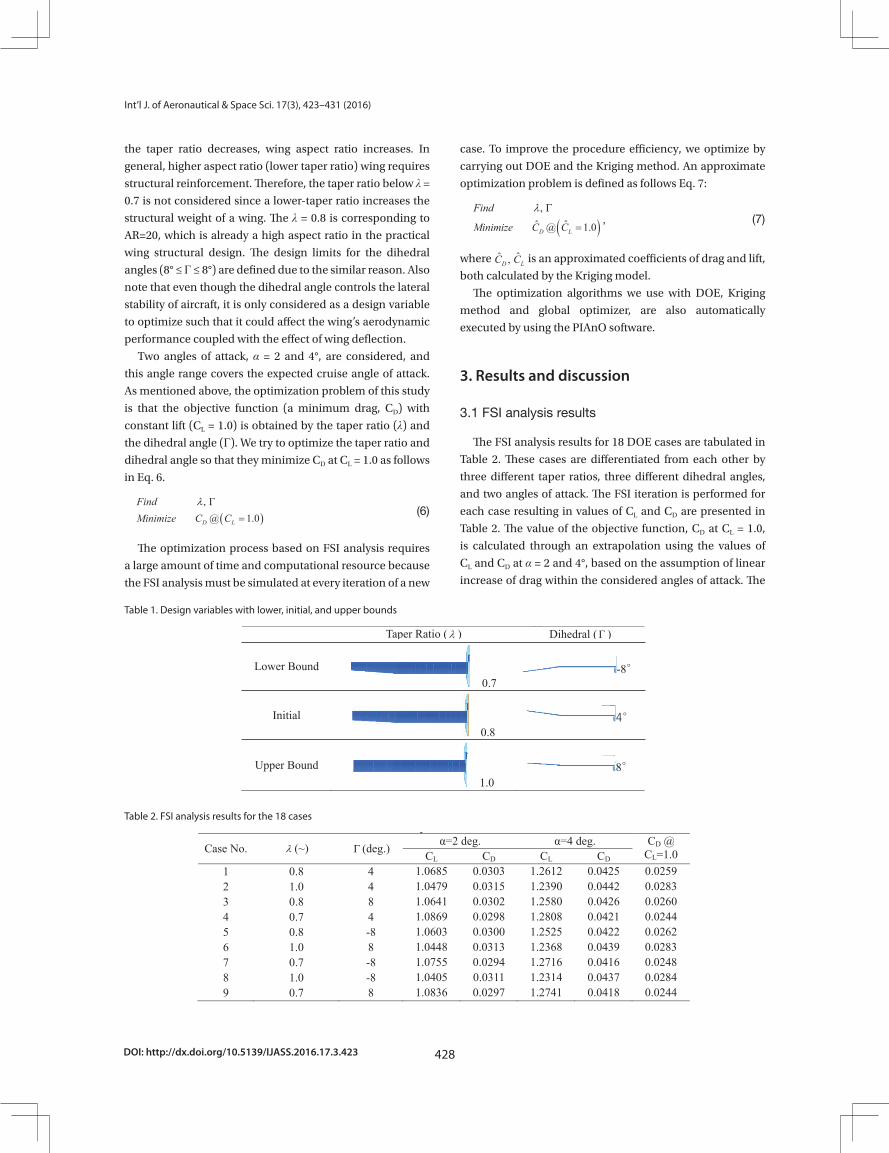
The FSI analysis results for 18 DOE cases are tabulated in

Table 2. These cases are differentiated from each other by

three different taper ratios, three different dihedral angles,

and two angles of attack. The FSI iteration is performed for

each case resulting in values of CL and CD are presented in

Table 2. The value of the objective function, CD at CL = 1.0,

is calculated through an extrapolation using the values of

CL and CD at α = 2 and 4°, based on the assumption of linear

increase of drag within the considered angles of attack. The

Table 1. Design variables with lower, initial, and upper bounds

18

Table 1. Design variables with lower, initial, and upper bounds Taper Ratio ( ) Dihedral ( )

Lower Bound 0.7

-8°

Initial 0.8

4°

Upper Bound 1.0

8°

Table 2. FSI analysis results for the 18 cases

19

Table 2. FSI analysis results for the 18 cases

Case No. (~) (deg.) α=2 deg. α=4 deg. CD @ CL=1.0 CL CD CL CD

1 0.8 4 1.0685 0.0303 1.2612 0.0425 0.0259 2 1.0 4 1.0479 0.0315 1.2390 0.0442 0.0283 3 0.8 8 1.0641 0.0302 1.2580 0.0426 0.0260 4 0.7 4 1.0869 0.0298 1.2808 0.0421 0.0244 5 0.8 -8 1.0603 0.0300 1.2525 0.0422 0.0262 6 1.0 8 1.0448 0.0313 1.2368 0.0439 0.0283 7 0.7 -8 1.0755 0.0294 1.2716 0.0416 0.0248 8 1.0 -8 1.0405 0.0311 1.2314 0.0437 0.0284 9 0.7 8 1.0836 0.0297 1.2741 0.0418 0.0244

429


http://ijass.org

values of the objective function serve as main data for design

optimization through the Kriging method.

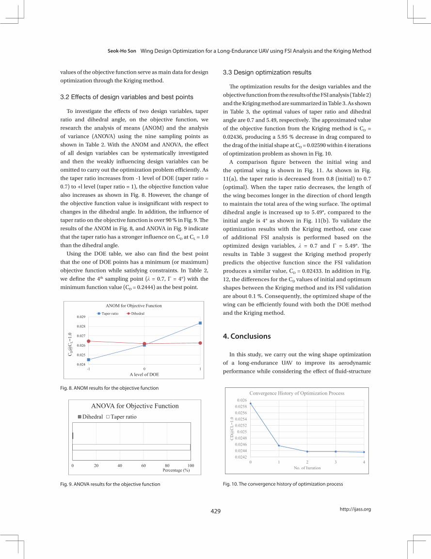
3.2 Effects of design variables and best points

To investigate the effects of two design variables, taper

ratio and dihedral angle, on the objective function, we

research the analysis of means (ANOM) and the analysis

of variance (ANOVA) using the nine sampling points as

shown in Table 2. With the ANOM and ANOVA, the effect

of all design variables can be systematically investigated

and then the weakly influencing design variables can be

omitted to carry out the optimization problem efficiently. As

the taper ratio increases from -1 level of DOE (taper ratio =

0.7) to +l level (taper ratio = 1), the objective function value

also increases as shown in Fig. 8. However, the change of

the objective function value is insignificant with respect to

changes in the dihedral angle. In addition, the influence of

taper ratio on the objective function is over 90 % in Fig. 9. The

results of the ANOM in Fig. 8, and ANOVA in Fig. 9 indicate

that the taper ratio has a stronger influence on CD at CL = 1.0

than the dihedral angle.

Using the DOE table, we also can find the best point

that the one of DOE points has a minimum (or maximum)

objective function while satisfying constraints. In Table 2,

we define the 4th sampling point (λ = 0.7, Γ = 4°) with the

minimum function value (CD = 0.2444) as the best point.

3.3 Design optimization results

The optimization results for the design variables and the

objective function from the results of the FSI analysis (Table 2)

and the Kriging method are summarized in Table 3. As shown

in Table 3, the optimal values of taper ratio and dihedral

angle are 0.7 and 5.49, respectively. The approximated value

of the objective function from the Kriging method is CD =

0.02436, producing a 5.95 % decrease in drag compared to

the drag of the initial shape at CD = 0.02590 within 4 iterations

of optimization problem as shown in Fig. 10.

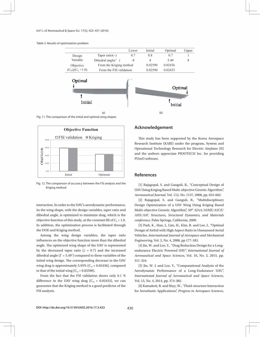
A comparison figure between the initial wing and

the optimal wing is shown in Fig. 11. As shown in Fig.

11(a), the taper ratio is decreased from 0.8 (initial) to 0.7

(optimal). When the taper ratio decreases, the length of

the wing becomes longer in the direction of chord length

to maintain the total area of the wing surface. The optimal

dihedral angle is increased up to 5.49°, compared to the

initial angle is 4° as shown in Fig. 11(b). To validate the

optimization results with the Kriging method, one case

of additional FSI analysis is performed based on the

optimized design variables, λ = 0.7 and Γ = 5.49°. The

results in Table 3 suggest the Kriging method properly

predicts the objective function since the FSI validation

produces a similar value, CD = 0.02433. In addition in Fig.

12, the differences for the CD values of initial and optimum

shapes between the Kriging method and its FSI validation

are about 0.1 %. Consequently, the optimized shape of the

wing can be efficiently found with both the DOE method

and the Kriging method.

4. Conclusions

In this study, we carry out the wing shape optimization

of a long-endurance UAV to improve its aerodynamic

performance while considering the effect of fluid-structure

28

Fig. 8. ANOM results for the objective function

0.024

0.025

0.026

0.027

0.028

0.029

-1 0 1

C D@

C L=1

.0

A level of DOE

ANOM for Objective Function

Taper ratio Dihedral

Fig. 8. ANOM results for the objective function

29

Fig. 9. ANOVA results for the objective function

0 20 40 60 80 100Percentage (%)

ANOVA for Objective FunctionDihedral Taper ratio

Fig. 9. ANOVA results for the objective function

30

Fig. 10. The convergence history of optimization process

0.02420.02440.02460.0248

0.0250.02520.02540.02560.0258

0.026

0 1 2 3 4

CD@

CL=1

.0

No. of Iteration

Convergence History of Optimization Process

Fig. 10. The convergence history of optimization process



interaction. In order to the UAV’s aerodynamic performance,

its the wing shape, with the design variables, taper ratio and

dihedral angle, is optimized to minimize drag, which is the

objective function of this study, at the constant lift of CL = 1.0.

In addition, the optimization process is facilitated through

the DOE and Kriging method.

Among the wing design variables, the taper ratio

influences on the objective function more than the dihedral

angle. The optimized wing shape of the UAV is represented

by the decreased taper ratio (λ = 0.7) and the increased

dihedral angle (Γ = 5.49°) compared to these variables of the

initial wing design. The corresponding decrease in the UAV

wing drag is approximately 5.95% (CD = 0.02436), compared

to that of the initial wing (CD = 0.02590).

From the fact that the FSI validation shows only 0.1 %

difference in the UAV wing drag (CD = 0.02433), we can

guarantee that the Kriging method is a good predictor of the

FSI analysis.

Acknowledgement

This study has been supported by the Korea Aerospace

Research Institute (KARI) under the program, System and

Operational Technology Research for Electric Airplane (II)

and the authors appreciate PIDOTECH Inc. for providing

PIAnO software.

References

[1] Rajagopal, S. and Ganguli, R., “Conceptual Design of

UAV Using Kriging Based Multi-objective Genetic Algorithm”,

Aeronautical Journal, Vol. 112, No. 1137, 2008, pp. 653-662.

[2] Rajagopal, S. and Ganguli, R., “Multidisciplinary

Design Optimization of a UAV Wing Using Kriging Based

Multi-objective Genetic Algorithm”, 50th AIAA/ASME/ASCE/

AHS/ASC Structures, Structural Dynamics, and Materials

conference, Palm Springs, California, 2009.

[3] Park, K., Han, J., Lim, H., Kim, B. and Lee, J., “Optimal

Design of Airfoil with High Aspect Ratio in Unmanned Aerial

Vehicles, International Journal of Aerospace and Mechanical

Engineering, Vol. 2, No. 4, 2008, pp 177-183.

[4] Jin, W. and Lee, Y., “Drag Reduction Design for a Long-

endurance Electric Powered UAV”, International Journal of

Aeronautical and Space Sciences, Vol. 16, No. 2, 2015, pp.

311-324.

[5] Jin, W. J. and Lee, Y., “Computational Analysis of the

Aerodynamic Performance of a Long-Endurance UAV”,

International Journal of Aeronautical and Space Sciences,

Vol. 15, No. 4, 2014, pp. 374-382.

[6] Kamakoti, R. and Shyy, W., “Fluid-structure Interaction

for Aeroelastic Applications”, Progress in Aerospace Sciences,

Table 3. Results of optimization problem

20

Table 3. Results of optimization problem Lower Initial Optimal Upper

Design Variable

Taper ratio(~) 0.7 0.8 0.7 1 Dihedral angle(°) -8 4 5.49 8

Objective (CD@CL =1.0)

From the Kriging method 0.02590 0.02436 From the FSI validation 0.02590 0.02433

31

(a) (b)

Fig. 11. The comparison of the initial and optimal wing shapes

(a) (b)Fig. 11. The comparison of the initial and optimal wing shapes

32

Fig. 12. The comparison of accuracy between the FSI analysis and the Kriging method

0.02

0.022

0.024

0.026

0.028

Initial Optimum

CD

@C

L(1.

0)

Objective Function

FSI validation Kriging

Fig. 12. The comparison of accuracy between the FSI analysis and the Kriging method

431


http://ijass.org

Vol. 40, 2004, pp. 535-558.

[7] Gonzalez, L.F., Walker, R., Srinivas, K. and Periaux, J.,

“Multidisciplinary Design Optimization of Unmanned Aerial

Systems (UAS) Using Meta Model Assisted Evolutionary

Algorithms”, 16th Australasian Fluid Mechanics Conference,

Gold Coast, Australia, 2007.

[8] Lee, S., Park, K., Kim, J., Jeon, S., Kim, K. and Lee, D.,

“Fluid-Structure Interaction and Design Optimization of

HAR Wing for Continuous 24-hour Flight of S-HALE Aircraft”,

the proceeding of KSAS, Vol. 4, 2012, pp. 121-126.

[9] Lam, X., Kim, A., Hoang, A. and Park, C., “Coupled

Aerostructural Design Optimization Using the Kriging Model

and Integrated Multiobjective Optimization Algorithm”,

Journal of Optimization Theory and Applications, Vol. 142,

2009, pp. 533-556.

[10] GAMBIT Software Package, Ver. 2.4.6, Ansys Fluent

Inc., Canonsburg, PA, USA

[11] TGRID Ver. 3.5, Ansys Fluent Inc., Canonsburg, PA, USA

[12] FLUENT Software Package, Ver. 6.3.26, Ansys Fluent

Inc., Canonsburg, PA, USA

[13] W. Jin. and Y. G. Lee, “Drag Reduction Design for

a Long-endurance Electric Powered UAV”, International

Journal of Aeronautical and Space Sciences, Vol. 16, No. 2,

2015, pp. 311-324.

[14] Diamond user manual, http://www.ipsap.snu.ac.kr,

2008.

[15] PIAnO (Process Integration, Automation and

Optimization) User’s Manual, Version 2.4, PIDOTECH Inc.,

2008.

[16] Son, S., Lee, S. and Choi, D., “Experiment-Based

Design Optimization of a Washing Machine Liquid Balancer

for Vibration Reduction”, International Journal of Precision

Engineering and Manufacturing, Vol. 13, No. 8, 2012, pp.

1433-1438.

[17] Forrester, A., Sobseter, A. and Keane, A., Engineering

Design via Surrogate Modeling, John Wiley & Sons, 2008.

[18] Advanced Aircraft Analysis software package, Ver. 3.2,

DARCorporation, Lawrence, KS, USA

wing design optimization for a long-endurance uav using...

Documents