guidance on systematic planning using the data quality ... · pdf filepreface . systematic...

United States Environmental Protection Agency

Office of Environmental Information Washington, DC 20460

EPA/240/B-06/001 February 2006

Guidance on Systematic Planning Using the Data Quality Objectives Process

EPA QA/G-4

FOREWORD

The U.S. Environmental Protection Agency (EPA) has developed the Data Quality Objectives (DQO) Process as the Agency’s recommended planning process when environmental data are used to select between two alternatives or derive an estimate of contamination. The DQO Process is used to develop performance and acceptance criteria (or data quality objectives) that clarify study objectives, define the appropriate type of data, and specify tolerable levels of potential decision errors that will be used as the basis for establishing the quality and quantity of data needed to support decisions. This document, Guidance on Systematic Planning Using the Data Quality Objectives Process (EPA QA/G-4), provides a standard working tool for project managers and planners to develop DQO for determining the type, quantity, and quality of data needed to reach defensible decisions or make credible estimates. It replaces EPA's August 2000 document, Guidance for the Data Quality Objectives Process (EPA QA/G-4), (U.S. EPA, 2000a) that considered decision-making only. Its presentation and contents are consistent with other guidance documents associated with implementing the Agency’s Quality System, all of which are available at EPA’s Quality System support Web site (http://www.epa.gov/quality).

As provided by EPA Quality Manual for Environmental Programs, EPA Manual 5360 (U.S. EPA, 2000c), this guidance is valid for a period of up to five years from the official date of publication. After five years, it will be reissued without change, revised, or withdrawn from the EPA Quality System series documentation.

Guidance on Systematic Planning Using the Data Quality Objectives Process provides guidance to EPA program managers and planning teams as well as to the general public where appropriate. It does not impose legally binding requirements and may not apply to a particular situation based on the circumstances. EPA retains the discretion to adopt approaches on a case-by-case basis that differ from this guidance if necessary. Additionally, EPA may periodically revise the guidance without public notice.

This document is one of the EPA Quality System Series documents which describe EPA policies and procedures for planning, implementing, and assessing the effectiveness of a quality system. Questions regarding this document or other EPA Quality System Series documents should be directed to:

U.S. EPA Quality Staff (2811R)

1200 Pennsylvania Ave, NW Washington, DC 20460

Phone: (202) 564-6830 Fax: (202) 565-2441 e-mail: [email protected]

Copies of EPA Quality System Series documents may be obtained from the Quality Staff or by downloading them from the Quality Staff Home Page: www.epa.gov/quality

EPA QA/G-4 i February 2006

http://www.epa.gov/quality

mailto:[email protected]

http://www.epa.gov/quality

EPA QA/G-4 ii February 2006

PREFACE

Systematic Planning Using the Data Quality Objectives Process provides information on how to apply systematic planning to generate performance and acceptance criteria for collecting environmental data. The type of systematic planning described is known as the Data Quality Objectives (DQO) Process. This process fully meets all aspects of the EPA Order 5360.1 A2, 2000, that establishes a Quality System for the Agency and organizations funded by EPA.

The DQO Process is a series of logical steps that guides managers or staff to a plan for the resource-effective acquisition of environmental data. It is both flexible and iterative, and applies to both decision-making (e.g., compliance/non-compliance with a standard) and estimation (e.g., ascertaining the mean concentration level of a contaminant). The DQO Process is used to establish performance and acceptance criteria, which serve as the basis for designing a plan for collecting data of sufficient quality and quantity to support the goals of the study. Use of the DQO Process leads to efficient and effective expenditure of resources; consensus on the type, quality, and quantity of data needed to meet the project goal; and the full documentation of actions taken during the development of the project.

This guidance document is intended for use by technical managers and Quality Assurance staff responsible for collecting data by: (1) providing basic guidance on applicable practices; (2) outlining systematic planning and developing performance or acceptance criteria; and (3) identifying resources and references that may be utilized by environmental professionals during the application of systematic planning.

The guidance discussed is non-mandatory and is intended to be a QA guide for project managers and QA staff in environmental programs to help them to better understand when and how quality assurance practices should be applied to the collection of environmental data.

EPA QA/G-4 iii February 2006

EPA QA/G-4 iv February 2006

TABLE OF CONTENTS Page

CHAPTER 0. INTRODUCTION................................................................................................1 0.1 EPA QUALITY SYSTEM ......................................................................................1 0.2 SYSTEMATIC PLANNING FOR ENVIRONMENTAL DATA

COLLECTION ........................................................................................................2 0.3 PERFORMANCE AND ACCEPTANCE CRITERIA............................................3 0.4 THE ELEMENTS OF SYSTEMATIC PLANNING ..............................................3 0.5 SYSTEMATIC PLANNING AND THE EPA INFORMATION QUALITY

GUIDELINES..........................................................................................................4 0.6 TYPES OF SYSTEMATIC PLANNING................................................................6 0.7 THE DQO PROCESS .............................................................................................7 0.8 BENEFITS OF USING THE DQO PROCESS.....................................................10 0.9 CATEGORIES OF INTENDED USE FOR ENVIRONMENTAL DATA .........11 0.10 ORGANIZATION OF THIS DOCUMENT .........................................................13

CHAPTER 1. STEP 1: STATE THE PROBLEM..................................................................15 1.1 BACKGROUND ...................................................................................................15 1.2 ACTIVITIES..........................................................................................................15 1.3 OUTPUTS..............................................................................................................18 1.4 EXAMPLES ..........................................................................................................18

CHAPTER 2. STEP 2: IDENTIFY THE GOALS OF THE STUDY ...................................21 2.1 BACKGROUND ...................................................................................................21 2.2 ACTIVITIES..........................................................................................................21 2.3 OUTPUTS..............................................................................................................25 2.4 EXAMPLES ..........................................................................................................25

CHAPTER 3. STEP 3: IDENTIFY INFORMATION INPUTS............................................27 3.1 BACKGROUND ...................................................................................................27 3.2 ACTIVITIES..........................................................................................................27 3.3 OUTPUTS .............................................................................................................29 3.4 EXAMPLES ..........................................................................................................29

CHAPTER 4. STEP 4: DEFINE THE BOUNDARIES OF THE STUDY...........................31 4.1 BACKGROUND ...................................................................................................31 4.2 ACTIVITIES..........................................................................................................32 4.3 OUTPUTS .............................................................................................................35 4.4 EXAMPLES ..........................................................................................................36

CHAPTER 5. STEP 5: DEVELOP THE ANALYTIC APPROACH...................................39 5.1 BACKGROUND ...................................................................................................39 5.2 ACTIVITIES..........................................................................................................39 5.3 OUTPUTS .............................................................................................................42 5.4 EXAMPLES ..........................................................................................................42

EPA QA/G-4 v February 2006

PageCHAPTER 6. STEP 6: SPECIFY PERFORMANCE OR ACCEPTANCE CRITERIA 45

6.1 BACKGROUND ...................................................................................................45 6.2 ACTIVITIES..........................................................................................................47

6.2.1 STATISTICAL HYPOTHESIS TESTING (STEP 6A) ............................47 6.2.2 ESTIMATION (STEP 6B) .......................................................................58

6.3 OUTPUTS .............................................................................................................67 6.4 EXAMPLES ..........................................................................................................68

CHAPTER 7. STEP 7: DEVELOP THE PLAN FOR OBTAINING DATA.......................71 7.1 BACKGROUND ...................................................................................................71 7.2 ACTIVITIES..........................................................................................................71 7.3 OUTPUTS .............................................................................................................78 7.4 EXAMPLES ..........................................................................................................78

CHAPTER 8. BEYOND THE DATA OBJECTIVES PROCESS .........................................81 8.1 PLANNING ........................................................................................................82 8.2 IMPLEMENTATION AND OVERSIGHT .........................................................83 8.3 ASSESSMENT......................................................................................................84

CHAPTER 9. ADDITIONAL EXAMPLES.............................................................................87 9.1 DECISIONS ON URBAN AIR QUALITY COMPLIANCE ...............................87 9.2 ESTIMATING MEAN DRINKING WATER CONSUMPTION RATES FOR

SUBPOPULATIONS OF A CITY ........................................................................93 9.3 HOUSEHOLD DUST LEAD HAZARD IN ATHINGTON PARK HOUSE, VA ......................................................................................................100

APPENDIX: DERIVATION OF SAMPLE SIZE FORMULA FOR TESTING MEAN OF NORMAL DISTRIBUTION VERSUS AN ACTION LEVEL ...............107

REFERENCES...........................................................................................................................111

EPA QA/G-4 vi February 2006

LIST OF FIGURES

Figure 1. EPA Quality System Components and ToolsPage

..................................................................2 Figure 2. The Data Quality Objectives (DQO) Process..................................................................8 Figure 3. How the DQO Process Can be Iterated Sequentially through the

Project Life Cycle............................................................................................................9 Figure 4. How Multiple Decisions May Be Organized to Solve a Hazard

Waste Investigation Problem.........................................................................................24 Figure 5. Influence Diagram Showing the Relationship of Estimated Lead Concentration

In Tap Water With other Important Study Inputs In Solving an Estimation Problem..25 Figure 6. An Example of How Total Study Error Can be Broken Down by Components...........47 Figure 7. Two Examples of Decision Performance Curves..........................................................52 Figure 8. An Example of a Decision Performance Goal Diagram Where the Alternative

Condition Exceeds the Action Level.............................................................................54 Figure 9. An Example of a Decision Performance Goal Diagram Where the Alternative

Condition Falls Below the Action Level .....................................................................54 Figure 10. The Project Life Cycle..................................................................................................81 Figure 11. The Data Quality Assessment Process .........................................................................85 Figure 12. Decision Performance Goal Diagram For the Urban Air Quality Compliance

Case Study ...................................................................................................................92Figure 13. Decision Performance Goal Diagram for Lead Dust Loading ...................................104

LIST OF TABLES Page

Table 1. Elements of Systematic Planning ....................................................................................3 Table 2. EPA General Assessment Factors....................................................................................5 Table 3. Commonalities Between EPA’s General Assessment for Evaluating the Quality of

Scientific and Technical Information and the Elements of Systematic Planning............6 Table 4. When Activities Performed Within the Systematic Planning Process Occur within the

DQO Process and/or the Project Life Cycle..................................................................11 Table 5. An Example of a Principal Study Question and Alternative Actions............................23 Table 6. Examples of Population Parameters and their Applicability to a Decision or Estimation Problem........................................................................................................41 Table 7. Statistical Hypothesis Tests Lead to Four Possible Outcomes ......................................49 Table 8. Elements of A Quality Assurance Project .....................................................................83 Table 9. False Acceptance Decision Plan Error Rates.................................................................93 Table 10. Number of Samples Required for Determining if the True Median Dust Lead

Loading is above the Standard ....................................................................................104

EPA QA/G-4 vii February 2006

GLOSSARY

AL Action Level CFR Code of Federal Regulations DEFT Decision Error Feasibility Trials DQA Data Quality Assessment DQI Data Quality Indicator DQO Data Quality Objective EPA Environmental Protection Agency GAF General Assessment Factor HVAC Heating, Ventilation and Air Conditioning IQG Information Quality Guideline MCL Maximum Contaminant Level MQO Measurement Quality Objective NAAQ National Ambient Air Quality NLLAP National Lead Laboratory Accreditation Program OMB Office of Management and Budget PBMS Performance-Based Measurement Systems PMSA Primary Metropolitan Statistical Area PMx Particulate Matter ( ≥x µm) ppb Parts per billion ppm Parts per million QA Quality Assurance QAPP Quality Assurance Project Plan QC Quality Control RCRA Resource Conservation Recovery Act SIP State Implementation Plan SOP Standard Operating Procedure SPC Science Policy Council TCLP Toxicity Characteristic Leaching Procedure UCL Upper Confidence Limit VOC Volatile Organic Compound VSP Visual Sample Plan WHO World Health Organization

EPA QA/G-4 viii February 2006

CHAPTER 0

INTRODUCTION

After reading this chapter, you should understand the basic structure of EPA’s Quality System, the general concepts of EPA’s Information Quality Guidelines, the role of systematic planning in the Quality System, the steps of the Data Quality Objectives (DQO) Process, and the benefits of applying the DQO Process for an environmental data collection project.

Unless some form of planning is conducted prior to investing the necessary time and resources to collect data; the chances can be unacceptably high that these data will not meet specific project needs. The hallmark of all successful projects, studies, and investigations is a planned data collection process that is conducted following the specifications given by an organization’s Quality System1. The Environmental Protection Agency (EPA) has established policy which states that before information or data are collected on Agency-funded or regulated environmental programs and projects, a systematic planning process must occur during which performance or acceptance criteria are developed for the collection, evaluation, or use of these data. For this reason, systematic planning is a key component of EPA's Quality System.

The Agency has issued Guidelines for Ensuring and Maximizing the Quality, Objectivity, Utility, and Integrity of Information Disseminated by the Environmental Protection Agency (IQGs) (U.S. EPA, 2002a), an integral component of the EPA’s Quality Program. The IQGs were developed by the Agency to comply with the 2001 Data Quality Act (February 2002), which directs OMB to provide “policy and procedural guidance to Federal Agencies for ensuring and maximizing the quality, objectivity, utility, and integrity of information, including statistical information, disseminated by Federal Agencies.” (Office of Management and Budget, 2001). Data collected according to the IQGs are in compliance with the Quality System and information on the guidelines may be obtained from www.epa.gov/quality/informationguidelines.

0.1 EPA Quality System

Policy and Program Requirements for the Mandatory Agency-Wide Quality System, EPA Order 5360.1 A2 (U.S. EPA, 2000b) and the applicable Federal regulations establish a Quality System that applies to all EPA organizations as well as those funded by EPA. It directs organizations to ensure that when collecting data to characterize environmental processes and conditions, these data are of the appropriate type and quality for their intended use. In addition, it directs that environmental technologies be designed, constructed, and operated according to defined expectations. In accordance with EPA Order 5360.1 A2, the Agency directs that:

Environmental programs performed for, or by, the Agency be supported by environmental data of an appropriate type and quality for their expected use. EPA

1 A Quality System is the means by which an organization ensures the quality of the products or services it provides and includes a variety of management, technical, and administrative elements such as policies and objectives, procedures and practices, organizational authority, responsibilities, and accountability.

EPA QA/G-4 1 February 2006

http://www.epa.gov/quality/informationguidelines

ASSESSMENT

defines environmental data as information collected directly from measurements, produced from models, or compiled from other sources such as databases or literature.

Decisions involving the design, construction, and operation of environmental technology be supported by appropriate quality-assured engineering standards and practices. Environmental technology includes treatment systems, pollution control systems and devices, waste remediation, and storage methods.

The Order is supported by the EPA Quality Manual for Environmental Programs, EPA Manual 5360 A1 (U.S. EPA, 2000c), which implements EPA’s Quality System.

EPA’s Quality System is divided into three types of components: Policy, Organization/ Program, and Project. Figure 1 illustrates the Project components, which include activities and tools which are applied or prepared for individual data collection projects to ensure that project objectives are achieved. More information on EPA’s Quality System is found in Overview of the EPA Quality System for Environmental Data and Technology (U.S. EPA, 2002b).

Systematic Planning

(e.g., DQO Process)

Data Verification

and Validation

Data Quality

Assessment

Defensible Products and Decisions

PLANNING IMPLEMENTATION

QA Project

Plan

Figure 1. Project Life Cycle Components

0.2 Systematic Planning for Environmental Data Collection

Systematic planning is a process based on the widely-accepted “scientific method” and includes concepts such as objectivity of approach and acceptability of results. The process uses a common-sense approach to ensure that the level of documentation and rigor of effort in planning is commensurate with the intended use of the information and the available resources. The systematic planning approach includes well-established management and scientific elements that result in a project’s logical development, efficient use of scarce resources, transparency of intent and direction, soundness of project conclusions, and proper documentation to allow determination of appropriate level of peer review.

Policy and Program Requirements for the Mandatory Agency-Wide Quality System, EPA Order 5360.1 A2 (U.S. EPA, 2000b) demands that systematic planning be used to develop “acceptance or performance criteria” for the collection, evaluation, or use of environmental data or information generated by, or on behalf of, the Agency. The document EPA Quality Manual for Environmental Programs, EPA Manual 5360 A1 (U.S. EPA, 2000c) further details the


elements of a systematic planning process and forms of documentation for the process, and it emphasizes the “specification of performance criteria for measuring quality” in the context of planning activities.

0.3 Performance and Acceptance Criteria

In general, performance criteria represent the full set of specifications that are needed to design a data or information collection effort such that, when implemented, generate newly-collected data that are of sufficient quality and quantity to address the project’s goals. Acceptance criteria are specifications intended to evaluate the adequacy of one or more existing sources of information or data as being acceptable to support the project’s intended use.

The DQO process is designed to generate performance criteria for the collection of new data. The generation of acceptance criteria will be discussed in the development of QA Project Plans (Guidance for Quality Assurance Project Plans EPA QA/G-5) (U.S. EPA, 2002d).

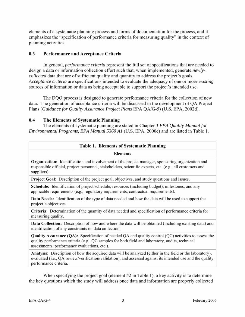
0.4 The Elements of Systematic Planning The elements of systematic planning are stated in Chapter 3 EPA Quality Manual for

Environmental Programs, EPA Manual 5360 A1 (U.S. EPA, 2000c) and are listed in Table 1.

Table 1. Elements of Systematic Planning Elements

Organization: Identification and involvement of the project manager, sponsoring organization and responsible official, project personnel, stakeholders, scientific experts, etc. (e.g., all customers and suppliers).

Project Goal: Description of the project goal, objectives, and study questions and issues.

Schedule: Identification of project schedule, resources (including budget), milestones, and any applicable requirements (e.g., regulatory requirements, contractual requirements).

Data Needs: Identification of the type of data needed and how the data will be used to support the project’s objectives.

Criteria: Determination of the quantity of data needed and specification of performance criteria for measuring quality.

Data Collection: Description of how and where the data will be obtained (including existing data) and identification of any constraints on data collection.

Quality Assurance (QA): Specification of needed QA and quality control (QC) activities to assess the quality performance criteria (e.g., QC samples for both field and laboratory, audits, technical assessments, performance evaluations, etc.).

Analysis: Description of how the acquired data will be analyzed (either in the field or the laboratory), evaluated (i.e., QA review/verification/validation), and assessed against its intended use and the quality performance criteria.

When specifying the project goal (element #2 in Table 1), a key activity is to determine the key questions which the study will address once data and information are properly collected


and analyzed. The manner in which study questions are framed will differ depending on whether the study is qualitative or descriptive in nature, will support the quantitative estimation of some unknown parameter, or will provide information for decision-making.

For qualitative projects, the study question may simply address what the information will be used to describe, for example:

• What is the state of nature in a particular location? • What species of invertebrates, emergent plants and algae are present in specified

locations along a watershed?

For quantitative projects involving estimation studies, the study question should include a statement of the unknown environmental (or other) characteristics (e.g., mean, median concentration) which will be estimated from the collected data. Choosing a well-defined parameter of interest leads to simplicity in data collection design. For example, to investigate what organic and inorganic air toxicants are present downwind from a smelter, the question should be framed in terms of the summary statistic (e.g. median) to be estimated.

For quantitative projects intended to test a specific preconceived theory, framing the study question typically leads to some type of statistical hypothesis test. For example, rather than using a model to estimate the mean concentration of air toxicants, the project may want to compare that concentration over time, or after some new pollution control device has been installed.

In all projects, it is important to concisely describe all information related to the project and to provide a conceptual model that summarizes information that is currently known and how this relates to the project’s goal. A concise summary of the underlying scientific or engineering theory should be appended to the information that describes the project’s goal to help facilitate any necessary peer review.

0.5 Systematic Planning and the EPA Information Quality Guidelines

The collection, use, and dissemination of environmental data and information of known and appropriate quality are integral to the Agency’s mission. The IQGs describe the Agency’s policies about the quality of information that the Agency disseminates. The IQGs apply to information generated by or for the Agency and also to information the Agency endorses, uses to develop a regulation or decision, or uses to support an Agency position. The IQGs also describe the administrative mechanisms by which affected parties may seek correction of information which they believe does not comply with OMB or EPA guidelines (U.S. EPA, 2002).

In order to assist in applying these guidelines, the EPA Science Policy Council (SPC) published A Summary of General Assessment Factors for Evaluating the Quality of Scientific and Technical Information (U.S. EPA, 2003) as part of the Agency’s commitment to enhance the transparency of EPA’s quality expectations for its information.


These factors apply to data and information generated under EPA’s Quality System as well as data and information voluntarily submitted by or collected from external sources. Although data from external sources may not have been collected according to specifications existing within EPA’s Quality System, EPA does apply appropriate quality controls when evaluating this information for use in Agency actions (U.S. EPA, 2003). When evaluating scientific and technical information, the SPC recommends using the five General Assessment Factors (GAFs) documented in Table 2.

Table 2. EPA General Assessment Factors Soundness: The extent to which the scientific and technical procedures, measures, methods or models employed to generate the information are reasonable for, and consistent with, the intended application.

Applicability and Utility: The extent to which the information is relevant for the Agency’s intended use.

Clarity and Completeness: The degree of clarity and completeness with which the data, assumptions, methods, quality assurance, sponsoring organizations and analyses employed to generate the information are documented.

Uncertainty and Variability: The extent to which the variability and uncertainty (quantitative and qualitative) in the information or the procedures, measures, methods or models are evaluated and characterized.

Evaluation and Review: The extent of independent verification, validation, and peer review of the information or of the procedures, measures, methods or models.

Using systematic planning to collect environmental information and data allows the project team to address all of the GAFs cited in Table 2. Although there is no direct one-to-one mapping between the eight elements of systematic planning (Table 1) and these five GAFs (Table 2), considerable commonalities do exist between them. Table 3 shows these major areas of commonality.

Some of these commonalities lead to the conclusions that:

• Achieving clarity in a project’s development becomes straightforward when using systematic planning, as almost every element of the planning process contributes to understanding how the project’s assumptions, methods, and proposed analyses will be conducted.

• Planning for analyzing the data and information before collection clearly meets the intent of the GAFs.

• Clear statements on the goals of the project developed through systematic planning leads to a better understanding of purpose and credibility of the results.

• Systematic planning leads to a clear statement of information needs and how the information will be collected, and leads to transparency in data quality.


• When performed correctly, systematic planning can fully address all questions raised by the GAFs, and it enables a project to fully meet the needs established by peer review policies.

Table 3. Commonalities Between EPA’s GAFs for Evaluating the Quality of Scientific and Technical Information and the Elements of Systematic Planning

GAFs

Soundness Applicability and Utility

Clarity and Completeness

Uncertainty and Variability

Evaluation and Review

Ele

men

ts o

f Sys

tem

atic

Pla

nnin

g

Organization Τ

Project Goal Τ Τ Τ

Schedule Τ

Data Needs Τ Τ Τ

Criteria Τ Τ

Data Collection Τ Τ Τ Τ

QA Τ Τ Τ

Analysis Τ Τ Τ Τ

0.6 Types of Systematic Planning

Various government agencies and scientific disciplines have established and adopted different variations to systematic planning, each tailoring their specific application areas. For example, the Observational Method is a variation on systematic planning that is used by many engineering professions. The Triad Approach, developed by EPA’s Technology Innovation Program, combines systematic planning with more recent technology advancements, such as techniques that allow for results of early sampling to inform the direction of future sampling. However, it is the Data Quality Objectives (DQO) Process that is the most commonly-used application of systematic planning in the general environmental community. Different types of tools exist for conducting systematic planning. The DQO Process is the Agency’s recommendation when data are to be used to make some type of decision (e.g., compliance or non-compliance with a standard) or estimation (e.g., ascertain the mean concentration level of a contaminant).


0.7 The DQO Process

The DQO Process is used to establish performance or acceptance criteria, which serve as the basis for designing a plan for collecting data of sufficient quality and quantity to support the goals of a study. The DQO Process consists of seven iterative steps that are documented in Figure 2. While the interaction of these steps is portrayed in Figure 2 in a sequential fashion, the iterative nature of the DQO Process allows one or more of these steps to be revisited as more information on the problem is obtained.

Each step of the DQO Process defines criteria that will be used to establish the final data collection design. The first five steps are primarily focused on identifying qualitative criteria, such as:

• the nature of the problem that has initiated the study and a conceptual model of the environmental hazard to be investigated;

• the decisions or estimates that need to be made and the order of priority for resolving them;

• the type of data needed; and • an analytic approach or decision rule that defines the logic for how the data will be used

to draw conclusions from the study findings.

The sixth step establishes acceptable quantitative criteria on the quality and quantity of the data to be collected, relative to the ultimate use of the data. These criteria are known as performance or acceptance criteria, or DQOs. For decision problems, the DQOs are typically expressed as tolerable limits on the probability or chance (risk) of the collected data leading you to making an erroneous decision. For estimation problems, the DQOs are typically expressed in terms of acceptable uncertainty (e.g., width of an uncertainty band or interval) associated with a point estimate at a desired level of statistical confidence.

• In the seventh step of the DQO Process, a data collection design is developed that will generate data meeting the quantitative and qualitative criteria specified at the end of Step 6. A data collection design specifies the type, number, location, and physical quantity of samples and data, as well as the QA and QC activities that will ensure that sampling design and measurement errors are managed sufficiently to meet the performance or acceptance criteria specified in the DQOs. The outputs of the DQO Process are used to develop a QA Project Plan and for performing Data Quality Assessment (Chapter 8).

The DQO Process may be applied to all programs involving the collection of environmental data and apply to programs with objectives that cover decision making, estimation, and modeling in support of research studies, monitoring programs, regulation development, and compliance support activities. When the goal of the study is to support decision making, the DQO Process applies systematic planning and statistical hypothesis testing methodology to decide between alternatives. When the goal of the study is to support estimation, modeling, or research, the DQO Process develops an analytic approach and data collection strategy that is effective and efficient.


Step 1. State the Problem. Define the problem that necessitates the study;

identify the planning team, examine budget, schedule

Step 2. Identify the Goal of the Study. State how environmental data will be used in meeting objectives and

solving the problem, identify study questions, define alternative outcomes

Step 3. Identify Information Inputs. Identify data & information needed to answer study questions.

Step 4. Define the Boundaries of the Study Specify the target population & characteristics of interest,

define spatial & temporal limits, scale of inference

Step 5. Develop the Analytic Approach. Define the parameter of interest, specify the type of inference,

and develop the logic for drawing conclusions from findings

Decision making (hypothesis testing)

Estimation and other analytic approaches

Step 6. Specify Performance or Acceptance Criteria

Specify probability limits for false rejection and false

acceptance decision errors

Develop performance criteria for new data being collected or acceptable criteria for existing data being considered for use

Step 7. Develop the Plan for Obtaining Data Select the resource-effective sampling and analysis plan

that meets the performance criteria

Figure 2. The Data Quality Objective Process


The DQO Process is flexible to meet the needs of any study, regardless of its size. Reflecting the common-sense approach to systematic planning, the depth and detail to which the DQO Process will be executed is dependent on the study objectives. For example, on a study having multiple phases, the DQO Process will allow the planning team to clearly separate and delineate data requirements for each phase.

For projects that require answers to multiple study questions, the resolution of one key question may support the evaluation of subsequent questions. In these cases, the DQO Process can be used repeatedly throughout the Project Life Cycle (Chapter 8). Often, the conclusions that are drawn early in such projects will be preliminary in nature, thereby requiring only limited initial planning and evaluation efforts. However, as the study nears completion and the consequences of drawing an incorrect conclusion become more critical, the level of effort needed to resolve the study questions generally will become greater. This iterative application of the DQO Process is illustrated in Figure 3.

ITERATE AS

NEEDED

START THE

DQO PROCESS

PRIM ARY STUDY

DECISION

STATE THE

PROBLEM

IDENTIFY GOALS OF THE STUDY

DEVELOP THE

ANALYTIC APPROACH

DEFINE THE

BOUNDARIES OF THE STUD Y

IDENTIFY INFORMATION

INPUTS

STATE THE

PROBLEM

DEVELOP DETAILED PLAN

FOR OBTAINING

DATA

IDENTIFY GOALS OF THE STUDY

DEVELOP THE ANALYTIC APPROACH

DEFINE THE

BOUNDARIES OF THE STUDY


INPUTS

STATE THE

PROBLEM

IDENTIFY GOALS OF

THE STUDY

DEVELOP THE

ANALYTIC APPROACH

DEFINE THE

BOUNDARIES OF THE STUDY

STUDY PLANNING COM PLETED



INTERM E-DIATE STUDY

DECISION ADVANCED

STUDY DECISION

DECIDE NOT

TO USE PROBABILISTIC

SAM PLING APPROACH

SPECIFY PERFORMANCE

OR ACCEPTANCE CRITERIA SPECIFY

PERFORMANCE OR

ACCEPTANCE CRITERIA SPECIFY

PERFORMANCE OR

ACCEPTANCE CRITERIA

DEVELOP DETAILED PLAN

FOR OBTAINING

DATA DEVELOP DETAILED PLAN

FOR OBTAINING

DATA


INPUTS

INCREASING LEVEL OF EFFORT

Figure 3. How the DQO Process Can be Iterated Sequentially Through the Project Life Cycle

Although statistical methods for developing the data collection design in Step 7 are strongly encouraged, not every problem can be resolved with probability-based sampling designs. On such studies, the DQO Process is still recommended as a planning tool, and the planning team is encouraged to seek expert advice on how to develop a non-statistical data collection design and how to evaluate the results of the data collection.

All of the activities that occur among the eight elements of the systematic planning process (Table 1) occur at some point within the DQO Process or later in the Project Life Cycle Components (Figure 1 and Chapter 8) as a result of performing the DQO Process, see Table 4.


0.8 Benefits of Using the DQO Process

During initial planning stages, a planning team can concentrate on developing requirements for collecting the data and work to reach consensus on the type, quantity, and quality of data needed to support Agency goals. The interaction amongst a multidisciplinary team results in a clear understanding of the problem and the options available. Organizations that have used the DQO Process have found the structured format facilitated good communications, documentation, and data collection design, all of which facilitated rapid peer review and approval.

• The structure of the DQO Process provides a convenient way to document activities and decisions and to communicate the data collection design to others.

• The DQO Process is an effective planning tool that can save resources by making data collection operations more resource-effective.

• The DQO Process enables data users and technical experts to participate collectively in planning and to specify their needs prior to data collection. The DQO Process helps to focus studies by encouraging data users to clarify vague objectives and document clearly how scientific theory motivating this project is applicable to the intended use of the data.

• The DQO Process provides a method for defining performance requirements appropriate for the intended use of the data by considering the consequences of drawing incorrect conclusions and then placing tolerable limits on them.

• The DQO Process encourages good documentation for a model-based approach to investigate the objectives of a project, with discussion on how the key parameters were estimated or derived, and the robustness of the model to small perturbations.

Upon implementing the DQO Process, your environmental programs can be strengthened in many ways, such as the following:

• Focused data requirements and an optimized design for data collection • Well documented procedures and requirements for data collection and evaluation • Clearly developed analysis plans with sound, comprehensive, QA Project Plans • Early identification of the sampling design and data collection process.


Table 4. When Activities Performed Within the Systematic Planning Process Occur Within the DQO Process and/or the Project Life Cycle

Activities Performed within the Systematic Planning Process (as featured

among the eight elements in Table 1)

When These Activities Occur Within the DQO Process and/or the Project Life Cycle

Identifying and involving the project manager/decision maker, and project personnel

Step 1. Define the problem

Part A of the Project Plan (Chapter 8)

Identifying the project schedule, resources, milestones, and requirements

Step 1. Define the problem

Describing the project goal and objectives Step 2. Identify the goal of the study

Identifying the type of data needed Step 3. Identify information needed for the study

Identifying constraints to data collection Step 4. Define the boundaries of the study

Determining the quality of the data needed Step 5. Develop the analytic approach Step 6. Specify performance or acceptance criteria Step 7. Develop the plan for obtaining data

Determining the quantity of the data needed Step 7. Develop the plan for obtaining data

Describing how, when, and where the data will be obtained

Step 7. Develop the plan for obtaining data

Specifying quality assurance and quality control activities to assess the quality performance criteria

Part B of the QA Project Plan (Chapter 8)

Part C of the QA Project Plan (Chapter 8)

Describing methods for data analysis, evaluation, and assessment against the intended use of the data and the quality performance criteria

Part D of the QA Project Plan (Chapter 8)

The Data Quality Assessment Process (Chapter 8)

0.9 Categories of Intended Use for Environmental Data

Throughout this document, the concept of intended use of the data is used to set the context for planning activities and focus the attention of the planning team. This guidance focuses on two primary types of intended use: decision-making and estimation. Details on each type and how they are related to some common analytic approaches (i.e., methodologies for using data to draw conclusions in support of the intended use) are as follows:

Decision making. Perhaps the most common category of intended use is decision making. In this context, decision making is defined as making a choice between two alternative conditions. At the time a decision maker chooses a course of action, the resulting consequences are usually unknown (to a greater or lesser degree) due to the uncertainty of future events. Therefore, a good decision maker should evaluate the likelihood of various future events and


assess how they might influence the consequences or “payoffs” of each alternative. This is where statistical methods help a decision maker structure the decision problem. The methodology of “classical” Neyman-Pearson statistical hypothesis testing provides a framework for setting up a statistical hypothesis, designing a data collection program that will test that hypothesis, evaluating the resulting data, and drawing a conclusion about whether the evidence is sufficiently strong to reject or (by default) accept the hypothesis, given the uncertainties in the data and assumptions underlying the methodology. The DQO Process has been designed to support a statistical hypothesis testing approach to decision making.

Other statistical methods can be used to support decision making. For example, Bayesian decision analysis provides a coherent framework for structuring a decision problem, eliciting a decision maker’s value preferences about uncertain outcomes, evaluating evidence from new data and information, and deciding whether to choose one of the alternatives now or continue to collect more information to reduce the uncertainty before deciding. This approach uses probabilities to express uncertainty and applies Bayes’ Rule to update the probabilities based on new information.

Estimation. Often the goal of a study is to evaluate the magnitude of some environmental parameter or characteristic, such as the concentration of a toxic substance in water, or the average rate of change in long-term atmospheric temperature. The resulting estimate may be used in further research, input to a model, or perhaps eventually to support decision making. However, the defining characteristic of an estimation problem versus a decision-making problem is that the intended use of the estimate is not directly associated with a well-defined decision.

Uncertainty in estimates is unavoidable due to a variety of factors, such as imperfect measurements, inherent variability in the characteristics of interest of the target population, and limits on the number or samples that can be collected. Statistical methods provide quantitative tools for characterizing the uncertainty in an estimate, and therefore play an important role in designing a study that will generate data of the right type, quality, and quantity.

The final sections of Chapters 1 through 7 illustrate how to apply each step of the DQO Process within the context of two examples that have been derived from real-life DQO development efforts. The same two examples are used within each chapter. Some background:

Example 1. Making Decisions About Incinerator Fly Ash for RCRA Waste Disposal

A waste incineration facility located in the Midwest routinely removes waste fly ash from its flue gas scrubber system and disposes of it in a municipal landfill. Previously the fly ash was determined not to be hazardous according to RCRA program regulations. The incinerator, however, recently began accepting and treating a new waste stream which may include, among other things, electrical appliances and batteries. For this reason, along with a recent change occurring in the incinerator process, the representatives of the incineration company are concerned that the fly ash associated with the new waste stream could contain hazardous levels of toxic metals, including cadmium. They have


decided to test the fly ash to determine whether it now needs to be sent to a hazardous waste landfill, or whether it can continue to be sent to the municipal landfill.

As a precursor to the DQO Process, the incineration company conducted a pilot study to determine the variability in the concentration of cadmium within loads of waste fly ash leaving the facility. From this pilot study, the company determined that each load is fairly homogeneous, but there is considerable variability among loads due to the nature of the waste stream. Therefore, the company decided that testing each container load before it leaves the facility would be an economical approach to evaluating the potential hazard. If the estimated mean cadmium level in a given container load was significantly higher than the regulated standards, then the container would be sent to a higher-cost RCRA landfill. Otherwise, the container would be sent to the municipal landfill.

Example 2. Monitoring Bacterial Contamination at Alki Beach

Citizens, city officials, and environmental regulators are concerned that individuals using a recreational beach (Alki Beach) on a river that flows through the city may be exposed to unacceptable levels of pathogens (disease-causing microorganisms) at certain points in time. A chicken farm is located close to the river about one mile upriver from Alki Beach. There is concern that heavy rainfall or other adverse events at this farm could result in discharge of chicken wastes into the river, and as a result, individuals using Alki Beach have the potential of being exposed to pathogens at health-threatening levels if there is inadequate monitoring of the beach waters.

At the present time, there is no beach water sampling program in place for Alki Beach. However, there is strong community support for developing a sampling program that would specify the type, number, location, and frequency of Alki Beach water samples to be collected and analyzed in order to yield an estimate of the density of pathogens present in beach waters (counts per 100mL).

This study will require the development of a beach water sampling plan and a means of estimating a specified parameter, calculated from the measured pathogen levels, which city health department staff can use with a predictive model to determine future actions. The scope of the DQO Process will focus on collecting information needed to estimate this parameter within an acceptable range of uncertainty.

0.10 Organization of This Document

The objective of this document is to describe how a planning team can use the DQO Process to generate a plan to collect data of appropriate quality and quantity for their intended use, whether it involves decision-making or simple estimation.

Following this introductory chapter, this document presents seven chapters (Chapters 1 through 7), each devoted to one of the seven steps of the DQO Process (Figure 2). Each chapter is divided into four sections:


Background — Provides background information on the specific step, including the rationale for the activities in that step and the objectives of the chapter. Activities — Describes the activities recommended for completing that step, including how inputs to the step are used. Outputs — Identifies the results that may be achieved by completing that step. Examples — Presents how the step is applied in the context of two different data collection examples, each focused on a different intended use (Section 0.11).

Chapter 8 shows how outputs of the DQO Process are used to develop a QA Project Plan and serves as important input to completing the remainder of the Project Life Cycle. Chapter 9 provides additional examples of implementing the DQO Process.


CHAPTER 1

STATE THE PROBLEM

1. State the Problem 2. Identify the Goal of the Study 3. Identify Information Inputs 4. Define the Boundaries of the Study 5. Develop the Analytic Approach 6. Specify Performance or Acceptance Criteria 7. Develop the Detailed Plan for Obtaining Data

The DQO Process 1. State the Problem y Give a concise description of the problem y Identify leader and members of the

planning team. y Develop a conceptual model of the

environmental hazard to be investigated. y Determine resources - budget, personnel,

and schedule.

After reading this chapter you should understand how to assemble an effective planning team and how to describe the problem and examine your resources for investigating it.

1.1 Background

The first step in any systematic planning process, and therefore the DQO Process, is to define the problem that has initiated the study. As environmental problems are often complex combinations of technical, economic, social, and political issues, it is critical to the success of the process to separate each problem, define it completely, and express it in an uncomplicated format. A proven effective approach to formulating a problem and establishing a plan for obtaining information that is necessary to resolve the problem is to involve a team of experts and stakeholders that represent a diverse, multidisciplinary background. Such a team would provide:

the ability to develop a concise description of complex problems, and multifaceted experience and awareness of potential data uses.

1.2 Activities

The most important activities in this step are to:

• describe the problem, develop a conceptual model of the environmental hazard to be investigated, and identify the general type of data needed;

• establish the planning team and identify the team’s decision makers; • discuss alternative approaches to investigation and solving the problem; • identify available resources, constraints, and deadlines associated with planning, data

collection, and data assessment.


The planning team will typically begin by developing a conceptual model of the problem, which summarizes the key environmental release, transport, dispersion, transformation, deposition, uptake, and behavioral aspects of the exposure scenario which underlies the problem. The conceptual model is an important tool for organizing information about the current state of knowledge and understanding of the problem, as well as for documenting key theoretical assumptions underlying an exposure assessment.

How do you establish the planning team and decision makers? The DQO planning team is typically composed of the project manager, technical staff, data users, and stakeholders. The development of a set of data quality objectives does not necessarily require a large planning team, particularly if the problem is straightforward. The size of the planning team is usually directly proportional to the complexity and importance of the problem. As the DQO Process is iterative, team members may be added to address areas of expertise not initially considered.

As the project manager is familiar with the problem and the budgetary/time constraints the team is facing, this person will usually serve as one of the decision makers and actively participate in all steps of the DQO Process. In cases where the decision makers or principal data users cannot attend team meetings, alternate staff members should attend and keep the decision makers informed of important planning issues.

Technical staff should include individuals who are knowledgeable about technical issues (such as geographical layout, sampling constraints, analysis, statistics, and data interpretation). Depending on the particular project, the planning team of multidisciplinary experts may include Quality Assurance managers, chemists, modelers, soil scientists, engineers, geologists, health physicists, risk assessors, field personnel, regulators, and data analysts with statistical experience. Often, a single person will have more than one required scientific background, and therefore, can represent multiple disciplines on the team.

Stakeholders are individuals or organizations that are directly affected by a decision or study result, may be interested in a problem, and want to be involved, offer input, or seek information. The involvement of stakeholders early in the DQO Process can provide a forum for communication as well as foster trust in the research or decision making process. The identification of stakeholders is influenced by the issues under consideration, but because EPA is organized into multiple program areas that are concerned with different environmental media that address different regulatory areas, identification of stakeholders is often not easy. EPA provides online guidance regarding stakeholder and public involvement in data collection programs at http://www.epa.gov/stakeholders.

How do you characterize the problem? As the problem is defined, important information from previous studies that solved similar problems, such as the performance of sampling and analytical methods, should be identified and documented. This information may prove to be particularly valuable later in the DQO Process. All relevant information and assumptions should be organized, reviewed, identified according to its source, and evaluated for its reliability. The planning team should be considerate of issues such as the regulatory requirements, organizations having an interest in the study, potential political issues associated with the study, non-technical


http://www.epa.gov/stakeholders

issues that may influence the sample design, and possible future uses of the data to be collected (e.g., the data to be collected may be eventually linked to an existing database).

It is critical to carefully develop an accurate conceptual model of the environmental problem, as this model will serve as the basis for all subsequent inputs and decisions. The conceptual model is often portrayed as a diagram that shows:

• known or expected locations of contaminants, • potential sources of contaminants, • media that are contaminated or may become contaminated, and • exposure scenarios (location of human health or ecological receptors).

Errors in the development of the conceptual model will be perpetuated throughout the other steps of the DQO Process and are likely to result in developing a sampling and analysis plan that may not achieve the data required to address the relevant issues.

It is important to identify theories and assumptions underlying the conceptual model to ensure adequate transparency. If the problem is complex, the team may consider breaking it into more manageable pieces, which might be addressed by separate studies. Priorities may be assigned to individual segments of the problem and the relationship between the segments examined.

What should be considered when identifying available resources, constraints, and deadlines? The planning team should identify and examine limitations that would be present on resources and time constraints associated with the process of collecting data and conducting activities that constitute the Project Life Cycle (Chapter 8). These activities would include completing the DQO Process (e.g., developing performance or acceptance criteria), preparing the QA Project Plan for collecting and analyzing samples, and interpreting and assessing the collected data. As far as possible, practical constraints such as right of entry, seasonality, or physical location affecting the taking of samples should be documented. The planning team should also examine available personnel and contracts (if applicable) and identify deadlines for collecting data.

How do you identify the type of intended use for the study data? At this point in the project, the planning team may be able to make a preliminary determination of the type of data needed and how it will be used. The two primary types of intended uses are decision making and estimation.

Sometimes the type of intended use will be obvious, such as when data are needed to determine whether a facility is in compliance with a regulatory limit. It is clear that these data would be used for decision making purposes. However, in other instances, the type of intended use may be difficult to identify this early in the process. For example, consider the situation where data are needed to support development of a regulation, which ultimately may involve making decisions about regulatory thresholds that reflect acceptable public health risks, as well as regulatory implementation structures. However, this early in the DQO Process, many of the regulatory alternatives may not yet be developed, and in fact, may depend on the findings of the study. Consequently, the intended use of the collected data may be to generate a set of estimates that will provide the scientific context in which alternatives can be developed later.


When identifying the intended use of the data, you may find it useful to consider the following questions:

• Are there alternative actions that can be clearly defined at this stage of the project, where the study results will guide the choice among those alternatives? If so, it is likely that this is a decision problem.

• Is this a research study that is trying to advance the state of knowledge by characterizing environmental conditions or trends? If so, this may be an estimation problem.

• Is this a study that will provide information about environmental conditions or trends to support the framing of regulatory alternatives? If so, this may be an estimation problem, although care should be taken to identify potential decisions that the study will directly support.

• Is this an environmental survey that is attempting to characterize levels of exposure for specific populations or areas? If so, and there are no existing statutes or regulations that will be applied to the results, then this may be an estimation problem. However, if the exposure levels will be compared to acceptable risk-based thresholds, then this may be a decision problem.

The project team also should try to identify whether the study will consider more sophisticated analytic approaches, such as Bayesian statistical methods or geostatistics. Those methods often involve adjustments to the activities within the DQO Process, which result in equivalent but different outputs. The earlier these methods are identified within the DQO Process, the more efficient the process will be.

1.3 Outputs

The major outputs of this step are:

• a concise description of the problem • a conceptual model of the environmental problem to be investigated with a preliminary

determination of the type of data needed and how it will be used; • a list of the planning team members and identification of decision makers or principal

data users within the planning team; and, • a summary of available resources and relevant deadlines for the study, including budget,

availability of personnel, and schedule.

1.4 Examples

Step 1 of the DQO Process for the two examples:

Example 1. Making Decisions About Incinerator Fly Ash for RCRA Waste Disposal Describing the problem. The problem is that a cost effective process needs to be developed to determine, on a container by container basis, whether fly ash generated


from the new waste stream needs to be sent to a RCRA landfill due to high levels of cadmium. The plant manager wants to avoid expensive RCRA disposal of waste, if possible, but also needs to comply with regulations and permits.

Establishing the planning team. The planning team includes the incineration plant manager (who will lead the team and be a decision-maker), a plant engineer, a quality assurance specialist with some statistical background, and a chemist with sampling experience in the RCRA program.

Describing the conceptual model of the potential hazard. The conceptual model describes waste fly ash that is created from industrial waste incineration and is a potential source of toxic metals that include cadmium. Fly ash is transferred to large disposal containers via a conveyer belt. These containers are filled and trucked to a disposal site. If the fly ash contains hazardous levels of toxic metals but is disposed in a municipal (sanitary) landfill, then these metals can leach into ground water and create runoff to streams and other surface water bodies, which could pose a hazard to human health and ecological receptors. If the hazardous waste were to be disposed in a RCRA approved landfill instead, then any such hazards would be contained.

The plant manager has determined that measurements of cadmium content of the waste fly ash need to be collected for each container load which the plant generates. These measurements will be used to make a decision on whether to have the load sent to a RCRA landfill or to the municipal landfill. The cost of sending a container to a municipal landfill is far less than a RCRA landfill, and this difference well exceeds the cost of data collection and analysis.

Identifying available resources, constraints, and deadlines. Although the project is not constrained by cost, the waste generator (the incineration company) wishes to hold sampling costs to below $2,500. The planning team has determined that company staff are available to perform the sampling, but they need to be properly trained in the techniques for performing this work. The company will need to contract with a laboratory that is qualified to perform the analysis using techniques that will be specified in Step 3 to determine cadmium levels in the collected ash samples and report results of the testing within one week.


Describing the problem. The primary problem is how to make timely (within 24 hours) and accurate assessments of the density of waterborne pathogens (bacteria, viruses, parasites) in Alki Beach waters on a routine basis. Data on the density of pathogens will be used to generate an estimate of a parameter which represents average pathogen level in the beach water.

Establishing the planning team. A five-member team has been selected to participate in the DQO Process, including the head of the city health department (who will lead the team), the staff member from the city health department who will be responsible for


managing the water monitoring program, a representative of the local citizens group, a biologist with experience in methods for collecting and measuring water samples for pathogens and indicators of pathogens, and the Deputy Manager of a local chicken farm having knowledge of operations which could lead to discharges into the river.

Describing the conceptual model of the potential hazard. The most likely source of potential acute pathogen contamination of beach waters is a chicken farm located one mile up-river from Alki Beach. Secondary sources may include unintentional sewer overflows, malfunctioning septic systems, and fecal contamination from other animals, all of which may have some access to the river. It is known that high rainfall can flush these pathogens from their source (e.g., chicken wastes and feces) into the river, thereby increasing the levels of pathogens present in river water. These levels arrive in waters at the beach area at a rate determined by the flow rate and depth of the river and flooding events can result in pathogens reaching greater areas of the beach.

People who use the beach following such contamination events include swimmers, boaters, and water skiers. However, swimmers are the focus of this sampling program due to their larger numbers and potential to be at greatest risk thorough accidental ingestion of the contaminated beach water.

Identifying available resources, constraints, and deadlines. The planning team determined that approved water sampling plan and pathogen estimation procedures need to be in place to allow the plan to be implemented by May 1 (i.e., the start of the recreational beach season). As Alki Beach is the only public-use beach on the river within city limits, sampling will be restricted to within the confines of the public beach area. Sampling methods and analysis will be conducted by city health department employees under a financial budget which city government has allocated to operate the monitoring program through September 15 (the end of the recreational beach season).

Looking Ahead to other DQO Steps: • Step 2 will clarify the principal study question and Step 3 will consider additional

uses of the data (e.g., links to databases). • The conceptual model will be used in Step 4, when establishing spatial boundaries

and considering regulatory and practical constraints for sampling.


CHAPTER 2

STEP 2. IDENTIFY THE GOALS OF THE STUDY


The DQO Process 2. Identify the Goal of the Study y Identify principal study question(s). y Consider alternative outcomes or actions

that can occur upon answering the question(s).

y For decision problems, develop decision statement(s), organize multiple decisions.

y For estimation problems, state what needs to be estimated and key assumptions.

After reading this chapter, you should know how to identify the principal study question, identify potential alternative actions with implications, and combine these to make statements on the decision or estimation problem.

2.1 Background

Step 2 of the DQO Process involves identifying the key questions that the study attempts to address, along with alternative actions or outcomes that may result based on the answers to these key questions. For decision-making problems, you should combine the information from these two items to develop a decision statement, which is critical for defining decision performance criteria later in Step 6. For estimation problems, you should frame the study with an estimation statement from which a set of assumptions, inputs, and methods are referenced.

On complex decision problems, you may identify multiple decisions that need to be made. These decisions are organized in a sequential or logical fashion within Step 2 and are examined to ensure consistency with the problem statement from Step 1. Similarly, large-scale or complex research studies may involve multiple estimators, and you will begin to determine how the different estimators relate to each other and to the overall study goal.

2.2 Activities

In this step you should:

• identify the principal study question and define alternative actions that may be taken based upon the range of possible outcomes that result from answering the principal study question;

• use the principal study question and alternative actions to make either a decision statement or estimation statement (whichever is relevant to the particular problem); and


• organize multiple decisions into an order of sequence or priority, and organize multiple estimation problems according to their influence on each other and their contribution to the overall study goals.

How do you identify the principal study question? Once the problem has been specified, you should formulate a principal study question. The principal study question will help focus the search for information that will address the study problem, and therefore, should be stated as specifically as possible. It will also help identify key unknown conditions or unresolved issues that will lead to finding a solution to the problem. The answer to the principal study question will provide the basis for deciding on a proper course of action to solve a decision problem or provide the missing information needed to make an accurate estimate on an estimation problem.

Initially, you should concentrate on specifying one principal study question, then later in the planning process, expand your consideration to other issues and questions. The following are examples of typical principal study questions:

Decision problems • Does the concentration of contaminants in ground water exceed acceptable levels? • Does the pollutant concentration exceed the NAAQ Standard? • Does a contaminant pose a human health or ecological risk? • Is the contaminant concentration significantly above background levels?

Estimation problems • What is the average rate of ground water flow in the aquifer? • What is the distribution of pollutant air concentrations over space and time? • What are the sizes of endangered species populations within the habitat of concern? • How many children in urban environments are exposed to unhealthy levels of airborne

pollutants? • How do the background contaminant concentrations vary over space and time?

What are alternative actions and how should you define them? Once the principal study question has been formulated, the planning team should identify a series of possible actions that may be taken once the question has been answered. In essence, the planning team will consider the range of potential answers to the principal study question, and then for each possible answer, will identify a logical course of action in response to that particular outcome. One such alternative may be to take no action. The team should confirm that the alternative actions can resolve the problem (if it exists) and determine whether the actions satisfy regulations. Table 5 gives an example of a principal study question and accompanying list of alternative actions.

For decision problems, how do you develop a decision statement? Once a list of alternative actions is compiled for a decision problem, this list and the principal study question are brought together to arrive at one or more decision statements that express choices to be made among alternative actions. The following template may be helpful in drafting a decision statement:


Determine whether …[some unknown environmental conditions/issues/criteria addressed by the principal study question] require (or support) …[taking one or more alternative actions].

Table 5. An Example of a Principal Study Question and Alternative Actions

Principal Study Question Alternative Actions

Are there significant levels of lead in floor dust at a residence, accompanied by deteriorated lead-based paint?

Remove any children from the residence and initiate lead-based paint abatement activities by certified workers.

Conduct lead-based paint interventions on selected painted building components followed by extensive dust cleaning.

Conduct specialized dust cleaning, provide educational materials to the household on cleaning techniques and other actions that will keep lead in dust to acceptable levels, and return in six months for more testing.

Take no action.

For estimation problems, how do you develop an estimation statement? For an estimation problem, one considers a range of potential outcomes associated with estimating some unknown entity that will address the study question. These outcomes may not directly lead to specific actions being taken, as in a decision problem, but they may be used to improve interpretation of other study results or to guide the subsequent investigation of other research or regulatory development issues. The spectrum of possible applications is so broad that a template for an estimation statement is not practical. Instead, these examples are offered as models:

• The principal quantity to be estimated is the distribution of concentrations of lead contamination in household tap water across a metropolitan area. We anticipate that there will be a significant proportion of non-detects, and that the highest concentrations will be correlated with the existence of lead service lines to the home. We do not anticipate any first-draw concentrations to exceed 1,000 ppm.

• Following an extensive renovation to a large apartment complex which occurred three years ago, it is desired to estimate the amount of time for which formaldehyde and other volatile organic compounds (VOCs) are now present at unhealthy levels in the air within selected housing units of the complex. We assume that levels will be at their peak in the early morning, when ventilation systems are on decreased rates during sleep periods. Measurements will be highly dependent on a building’s HVAC system, certain unit-specific properties such as relative humidity, and the behavior patterns of the occupants. We do not anticipate levels will exceed regulatory standards.

• A State wishes to assess a given water body relative to the presence of nutrient impairment and how average nutrient concentrations are changing over time. Seasonal peaks occur in nutrient concentrations and will need to be considered in the sampling and


estimation process, along with other climatic impacts. Estimation techniques will need to address nutrient measurements that cover several orders of magnitude.

Does the DQO Process address multiple decisions? For some complex decision problems, more than one decision statement may be necessary to formulate, implying that several decisions would need to be made in order to solve the problem. You need to examine how each decision relates to others and make a list of priorities for resolving the problem. An example of the prioritizing process associated with a hazardous waste investigation is presented in Figure 4.

D es ig n a n d Im p le m e n t S ite In v es tig a tio n

D o e s S u r f a c e S o i l P o s e

U n a c c e p t a b le R is k ?

D o es S u b s u r f ac e

S o i l P os e U n ac c e p ta b le

R is k ?

D o e s G r o u n d w a te r

P os e U n a c c e p t a b le

R is k ?

N o fu r th e r ac tio n

N o f u r th e r a c t io n


Is S u b s u r f ac e S o i l S o u rc e o f

G W C o n ta m in a t io n ?

D es ig n & Im p le m e n t S u r f ac e

S o i l R e m e d ia t io n

D es ig n & Im p le m e n t

S u b s u r f ac e S o il R em e d ia t io n

D e s ig n & Im p le m e n t

In te g r a t e d P la n f o r R e m e d ia t io n

D e s ig n & Im p le m e n t G r o u n d

W ate r R e m e d ia t io n

W e re S u r f a c e S o i l C le a n u p

W ere G r o u n d W a te r C le a n u p

W e re S u b s u r f ac e S o il

N o N o N o

N oN o

N o N o N o

Y e s

Y e s Y e s

C le a n u p G o a ls G o a ls M e t ? M e t?

G o a ls M e t ?


Y e s Y e s

Figure 4. How Multiple Decisions Can Solve a Hazard Waste Investigation Problem

Does the DQO Process address multiple estimates? Similarly, large and/or complex estimation problems may require that estimates be made of multiple parameters and combined to address the overall problem. Depending on the nature of the problem and how the estimates need to be combined with other important information, more information and precision may be required for certain estimates. It may be helpful to show the relationships among the different estimators and input variables by developing a diagram, such as the influence diagram in Figure 5.


Lead concentration

at tap

Service line material (lead or not)

Distance to drinking water

plant

Water treatment methods

Predictive model of lead concentration

Occupant age

distribution

Drinking water standard

Estimate of health risk

Risk management strategy (future)

Figure 5. Influence Diagram Showing the Relationship of Estimated Lead Concentration in Tap Water with Other Important Study Inputs in Solving an Estimation Problem

2.3 Outputs

The principal outputs at the end of this step are:

• A well-defined principal study question, • A listing of alternative outcomes or actions as a result of addressing the principal

study questions, • For decision problems, a list of decision statements that address the study

question, and • For estimation problems, a list of estimation statements that address the study

question.

2.4 Examples

The specific decision and estimation statements that result from Step 2 are:



Specifying the primary question. The primary question to be addressed is the following:

Does a given container of waste fly ash contain mean levels of cadmium that exceed the regulatory standard, thereby requiring it to be disposed in a RCRA landfill?

Determining alternative actions. Possible alternative actions are as follows:

• Take no action (e.g., data are inconclusive) • Dispose of the container in a RCRA landfill. • Dispose of the container in a sanitary landfill.

Specifying the decision statement. The decision statement is as follows:

• Determine whether the container of fly ash is required to be sent to the RCRA landfill or can be disposed in the municipal landfill.


Specifying the principal study question. After receiving input from citizens, the planning team developed and documented the primary study question:

• At various times during the study timeframe,, what is a reasonable estimate of the density of aquatic pathogens present in the water at Alki Beach?

Specifying the estimation statement. The principal estimation measure will be some average measure of the pathogen density, along with an upper confidence limit calculated on this measure to reflect uncertainty. The upper confidence limit provides additional assurance that the magnitude of the pathogen level in the water is properly captured. The process of estimating these parameters will need to properly account for the underlying distribution of measurements and the handling not-detected measures.

Looking Ahead to other DQO Steps: • The principal study question is used to determine appropriate inputs

needed to resolve the problem in Step 3 and to identify the specific population parameters in Step 5.

• On decision problems, the principal study question also helps determine the baseline and alternative conditions in Step 6.

• On decision problems, alternative actions will form the basis for determining the potential consequences of committing a decision error, as addressed in Step 6.


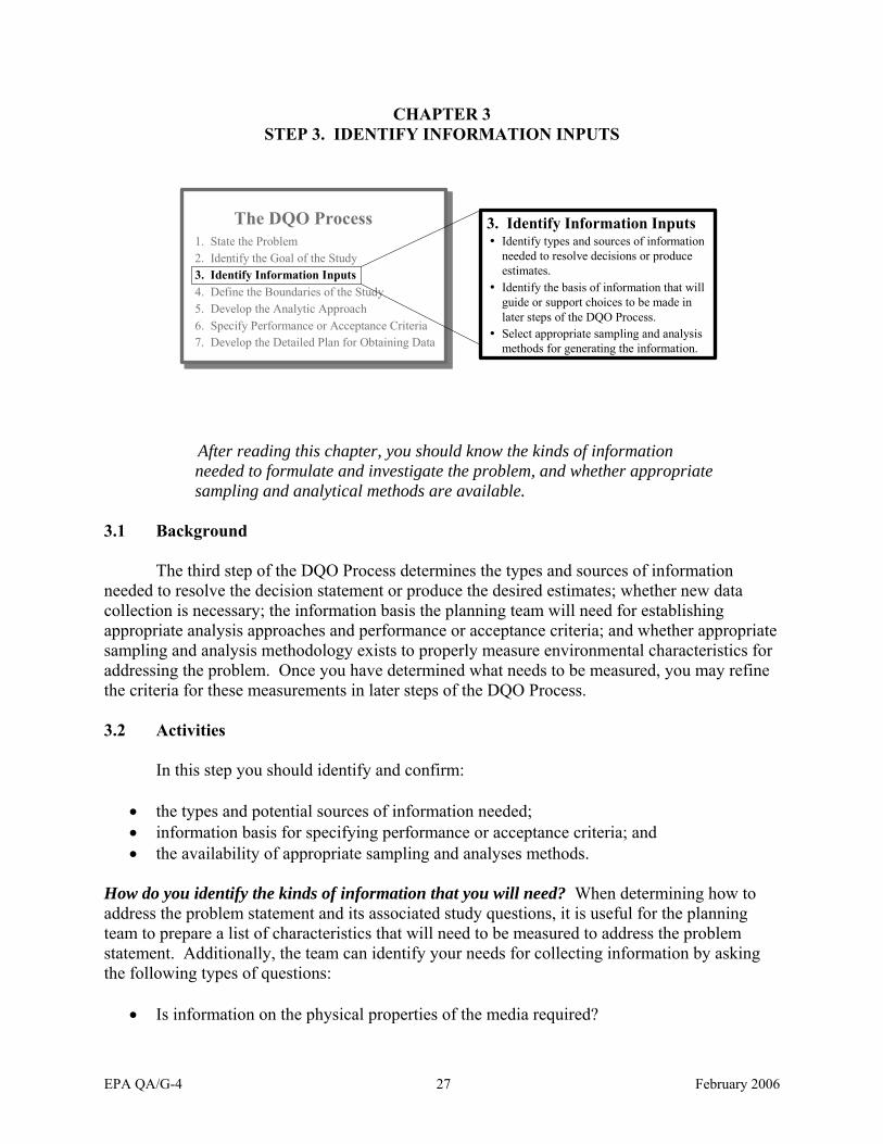
CHAPTER 3 STEP 3. IDENTIFY INFORMATION INPUTS


The DQO Process 3. Identify Information Inputs y Identify types and sources of information

needed to resolve decisions or produce estimates.

y Identify the basis of information that will guide or support choices to be made in later steps of the DQO Process.

y Select appropriate sampling and analysis methods for generating the information.

After reading this chapter, you should know the kinds of information needed to formulate and investigate the problem, and whether appropriate sampling and analytical methods are available.

3.1 Background

The third step of the DQO Process determines the types and sources of information needed to resolve the decision statement or produce the desired estimates; whether new data collection is necessary; the information basis the planning team will need for establishing appropriate analysis approaches and performance or acceptance criteria; and whether appropriate sampling and analysis methodology exists to properly measure environmental characteristics for addressing the problem. Once you have determined what needs to be measured, you may refine the criteria for these measurements in later steps of the DQO Process.

3.2 Activities

In this step you should identify and confirm:

• the types and potential sources of information needed; • information basis for specifying performance or acceptance criteria; and • the availability of appropriate sampling and analyses methods.

How do you identify the kinds of information that you will need? When determining how to address the problem statement and its associated study questions, it is useful for the planning team to prepare a list of characteristics that will need to be measured to address the problem statement. Additionally, the team can identify your needs for collecting information by asking the following types of questions:

• Is information on the physical properties of the media required?


• Is information on the chemical characteristics of the matrix needed? • Can existing data be used to make the decision or produce the estimate? • Do we need to collect new measurements on environmental characteristics?

What issues should you consider when determining whether existing data may possibly serve as a source of information? If you can address your problem in part through the use of an existing data set, then you should inquire about its quality assurance and control information to assess whether the data will satisfy your needs. If you integrate newly-collected data with existing data, then the methods used to generate the existing data will need to be examined in order to ensure that new data are generated using appropriate methods.

How do you identify the information basis for later specification of performance or acceptance criteria? In Step 5 of the DQO Process, the planning team should agree upon an approach to analyzing information obtained when studying and drawing conclusions from this analysis; while in Step 6, the team should specify the performance or acceptance criteria which the data need to achieve for your particular intended use on the study. At these stages, you will need to identify the basis for the information that will guide or support the specific choices and decisions which the planning team will make in these later steps.

On decision problems, the analytic approach will involve developing a decision rule that incorporates some type of Action Level. An Action Level represents a threshold value that is primarily used to determine which Step 2 alternative actions should be pursued. The specific information source for determining the Action Level is identified within this step of the DQO Process. The actual numerical value of the Action Level need not be specified until Step 5.

If instead of an Action Level, a decision will be made relative to some type of background concentration, then you should determine the information basis for characterizing background. These characteristics need to be consistent with those of the area to be investigated.

What types of considerations should be noted when identifying and evaluating appropriate sampling and analysis methods? Using the list of environmental characteristics that are necessary for addressing a particular decision or estimate, the planning team should develop a list of existing physical sampling and analytical methods that would be appropriate for obtaining the necessary information. If no such methods can be identified, then it may be necessary for the planning team to return to Step 2 to determine a slightly different set of goals.

On decision problems, the decision performance goals to be established in Step 6 will rely on bias being kept to a minimum. Major causes of bias for environmental sampling and analysis include (1) non-representative sampling; (2) instability or contamination of samples between sampling and analysis; (3) interferences and matrix effects in analysis; (4) inability to determine the relevant forms of the parameter being measured; (5) calibration; and (6) failure to blank-correct. Some methods are particularly subject to bias in calibration and should be avoided if possible. The use of certified personnel and accredited laboratories or Performance-Based Measurement Systems (PBMS) is also noted in this step.


3.3 Outputs

The outputs from Step 3 are:

• lists of environmental characteristics that will resolve the decision or estimate and potential sources for the desired information inputs;

• information on the number of variables that will need to be collected; • the type of information needed to meet performance or acceptance criteria; • information on the performance of appropriate sampling and analysis methods.

3.4 Examples

For the two examples, the Step 3 activities are:


Identifying the type of information that is needed to resolve the decision statement. This is a new data collection effort, with analyses being performed on fly ash samples collected from newly-generated container loads. The planning team has decided to measure cadmium concentration in samples which have gone through the EPA’s standard Toxicity Characteristic Leaching Procedure (TCLP) extraction technique.

Identifying the source of information. Data from the existing pilot study will provide preliminary information on within-container and between-container variability in sample measurements which will be important to preparing a sampling plan.

Identifying how the Action Level will be determined. In addition to impacting the analytic approach to be used, RCRA solid and hazardous waste program regulations will dictate the Action Level which will lead to resolution of the decision statement. The Action Level will be based on RCRA toxicity regulations for cadmium in TCLP leachate.

Identifying appropriate sampling and analysis methods. Cadmium will be measured in TCLP leachate according to the method specified in 40 CFR 261, App. II. The detection limit associated with this method is expected to be well below the Action Level that will be used.


Identifying the types of information that are needed. As Alki Beach is a fresh water body, the planning team used recommendations from EPA to decide that measurements on the density of Escherichia coli (E. coli) and enterococci in collected water samples would be used as indicators when estimating the density of pathogens in Alki Beach waters. Additional information which the planning team determined were needed to develop the sampling plan includes:


• regulatory guidance on the average densities of E. coli and enterococci, • EPA-recommended methods for collecting and analyzing samples of beach water, • the speed and route of major currents and physical characteristics of the beach, • density data for E. coli and enterococci that are available for similar beaches.

Identifying the source of information. Information beyond the collection of new data will be obtained from various data sources including city and state agencies, the EPA, and members of the planning team.

Identifying appropriate sampling and analysis methods. Sample and analytical specifications must be appropriate to ensure that measurements can be quantified accurately at levels below the water quality criteria that the EPA or state previously issued under Section 304 of the Clean Water Act.

Each water sample bottle will be one liter in volume and will be filled with beach water such that water enters the bottle at a specified depth below the surface of the water. Studies conducted at river beaches similar to Alki Beach indicate that measurements of pathogens at a 0.3 meter depth correlate well with health effects.

The planning team indicated that it would be highly desirable for the laboratory to process, measure and report the density measurements for all samples collected on a given day within 24 hours. This rapid turn-around of information will facilitate the city health department’s use of the predictive model for the users of Alki Beach. Therefore, an analytical method based on molecular polymerase chain reaction was chosen to ensure that samples can be analyzed and measurements of the two indicators reported within the desired time period.

Looking Ahead to other DQO Steps: • The parameter of interest will be selected in Step 5 together with the

type of inference needed. These issues are also considered in Steps 7. • Criteria for existing data will be examined in Step 7. • Method detection limit and method quantification limits identified in

this step will be revisited in Step 7.


CHAPTER 4

STEP 4. DEFINE THE BOUNDARIES OF THE STUDY


The DQO Process 4. Define the Boundaries of the Study y Define the target population of interest

and its relevant spatial boundaries. y Define what constitutes a sampling unit. y Specify temporal boundaries and other

practical constraints associated with sample/data collection.

y Specify the smallest unit on which decisions or estimates will be made.

After reading this chapter you should understand how to define the target population, the geographic (spatial) and temporal boundaries associated with the population, how to examine any practical constraints to collecting data, and factors that affect your selection of the unit which defines the scale of sampling and the scale of decision making or estimation.

4.1 Background

In Step 4 of the DQO Process, you should identify the target population of interest and specify the spatial and temporal features pertinent for decision making or estimation.

The target population refers to the total collection or universe of sampling units to be studied and from which samples will be drawn. If the target population consists of “natural” entities (e.g., people, plants, or fish), then the definition of sampling unit is straightforward, it is the entity itself. When the target population consists of continuous media, such as air, water, or soil, the sampling unit must be defined as some area, volume, or mass that may be selected from the target population. When defining sampling units, you should ensure that the sampling units are mutually exclusive (i.e., they do not overlap), and are collectively exhaustive (i.e., the sum of all sampling units covers the entire target population). The actual determination of the appropriate size of a sampling unit, and of an optimal quantity of sample support for environmental data collection efforts can be complicated, and usually will be addressed as a part of the sampling design in Step 7. Here in Step 4, the planning team should be able to provide a first approximation of the sampling unit definition when specifying the target population.

Practical constraints that could interfere with sampling should also be identified in this step. A practical constraint is any hindrance or obstacle (such as fences, property access, water bodies) that may interfere with collecting a complete data set. These constraints may limit the


spatial and/or temporal boundaries or regions that will be included in the study population and hence, the inferences (conclusions) that can be made with the study data.

You also should determine the scale of inference for decisions or estimates. The scale of inference is the area or volume, from which the data will be aggregated to support a specific decision or estimate. For example, a decision about the average concentration of lead in surface soil will depend on area over which the data are aggregated, so you should identify the size of decision units for this problem. A decision or estimate on each piece of land may lead to the recommendation of a specific size such as a half-acre area (equivalent to a semi-urban home area) for the sampling unit.

4.2 Activities

In this step you should:

• define the target population, • determine the spatial and temporal boundaries, • identify practical constraints, and • define the scale of inference (i.e., decision unit or scale of estimation).

How do you define the target population? This is the total collection of sample units. It may be helpful to “work backwards” and think of how you would define an individual sampling unit when trying to develop a clear definition of the target population. For example, if a 6 inch core is to be sent to the laboratory for analysis, the target population would be all possible 6 inch cores from the area under investigation.

What types of boundaries on sampling from the target population are important to characterize? As the target population is defined, two types of boundaries that must be considered when sampling from this target population are characterized:

• spatial boundaries that define the physical area to be studied and generally where samples will be collected, and

• temporal boundaries that describe the time frame that the study will represent and when the samples should be taken.

Defining boundaries carefully can also prevent the inappropriate combining of disparate data sets that could mask useful information.

How do you determine spatial boundaries on the target population? The conceptual model developed in Step 1 of the DQO Process will provide essential input into defining the spatial boundaries. Important considerations for defining the spatial boundaries are:

1. Define the geographic area applicable for the decision making or estimation.

You should define the entire geographical area where the data are to be collected using unambiguous location coordinates (such as latitude, longitude, and elevation) or distinctive


physical features described in terms of length, area, volume, or legal boundaries. It is important to state as definitively as possible the media and geographic area; this statement may include soil depth, water depth, or distance inside a fence line. Some examples of geographic areas are the soil within the property boundaries down to a depth of 6 inches, a specific water body, or the natural habitat range of a particular animal species. You should be careful when designating areas that are on the periphery of the geographic area because peripheral samples are subject to edge effects (the influence of factors not under this investigation upon the sampling units).

2. Divide the population into subsets that have relatively homogeneous characteristics.

It is often appropriate to consider dividing the target population into subpopulations that are relatively homogeneous within each area or subunit. The planning team should use its knowledge of the conceptual model (Step 1) to consider how the characteristics of interest for the target population vary or change over space and time. When combined with an appropriate sampling design in Step 7, this approach can reduce the number of samples required to meet the performance or acceptance criteria (Step 6), and, thus, allow more efficient use of resources.

How do you determine the temporal boundaries of the decision statement? Important considerations for defining the temporal boundaries are:

1. Determine the period of time the data should represent.

Conditions may vary over the course of a study because of time-related phenomena such as weather conditions, seasons, operation of equipment under different environmental conditions, or activity patterns. Examples of these variations include seasonal ground water levels, daily or hourly airborne contaminant levels in metropolitan areas, and fluctuations in pollutant discharges from industrial sources. You should determine when conditions are most favorable for collecting data that are representative of the target population, and select the most appropriate time period to collect data. For example,

• measurement of lead in dust on window sills may show higher concentrations during the summer when windows are raised and paint/dust accumulates on the window sill;

• measurement of pesticides on surfaces may show greater variations in the summer because of higher temperatures and volatilization;

• measurements of airborne particulate matter may not be accurate if the sampling is conducted in the wetter winter months rather than the drier summer months.

2. Determine the time frame for which the decision or estimate is relevant.

It may not be possible to collect data over the full time period to which the decision or estimate will apply. This is particularly true when data are used to make decisions that impact the future of the target population, such as the future use of a brownfield (i.e., an inactive property being put back into productive economic use after the contaminants once present at the property no longer pose an unacceptable risk to human health or to the environment). You should evaluate the population and determine the optimum time frame for collecting data, given that the medium may change over time, or the time constraints of the study relative to the


decision or estimate to be made. You should define time frames for the overall population and for any subpopulation of interest, then address discrepancies that may arise from the short time frame of data collection relative to the long time periods for implementing decisions. For example, you may develop a decision or estimation statement that is based on:

• the condition of contaminant leaching into ground water over a period of a hundred years, or

• the risk conditions of an average resident over their average length of residence, which is estimated to be eight years.

What kinds of practical constraints on collecting data should you identify? These constraints could include access to the property, availability and operation of equipment, and environmental conditions when sampling is not possible (high humidity, freezing temperatures). For example, it may not be possible to take surface soil samples beyond the boundaries of a property under investigation because permission has not been granted by the owner of the adjacent property. As another example, it may not be possible to collect dust wipe samples for lead analysis if certified inspectors are not available to supervise the sampling.

How do you define the scale of inference for decision or estimation problems? The scale of inference refers to the manner to which the planning team has delineated the smallest unit of area, volume, or time over which data will be collected, analyzed, aggregated, and interpreted to make a decision (and therefore control decision errors) or to produce an estimate (and therefore control the precision of the estimate). The consequences of making incorrect decisions or arriving at estimates with unacceptable uncertainty (Step 6) are linked to the size, location, and shape of the decision unit or scale of estimation.

For decision problems, it is important to consider present and future uses for the decision unit, where the decision unit is located (remote area versus densely populated area) and requirements for potential remediation. The consequences of a wrong decision (even if quite small) should be carefully considered. For example, if collected data lead to a decision to clean a large land area (soil removed to a certified disposal area), then if true (unknown) conditions would not have warranted such an action, the decision maker would incur a large cost unnecessarily. The area of land being sampled (i.e., the size of the decision unit) should match the potential risk associated with making an incorrect decision. Therefore, when establishing the scale of decision making, the scale should not be set so large that an incorrect decision could result in an unacceptable resource expense, or so small that an incorrect decision would pose an unacceptable threat to human health or the environment.

For estimation problems, the scale of inference usually will be linked to the goals of the study and potential uses of the study results, in terms of either follow-on research or subsequent decision making. While it may be difficult to identify the specific consequences of making inaccurate estimates, usually you can express an amount of lost time and resources that would occur if a particular estimate is found to be inadequate, and as a result, a certain component of the study needs to be redone.


What more guidance can you provide on establishing a scale of decision making? For a decision making problem that involves multiple decisions, the planning team should address the question of how properly to control the error rate associated with making multiple decisions.

The planning team may establish decision units based on several considerations:

• Risk – The scale of decision making based on risk is determined by the potential exposure that an area presents. For example, a geographic area may defined as the top six inches of soil within the property boundaries, and the population would be the collection of individual volumes of soil that could be selected for inclusion in a sample. The scale of decision making could be the size that corresponds to the area where children derive the majority of their exposure, such as a play area or an average residential lot size if the future land use will be residential. Studying the area at this scale would be sufficiently protective of children, given their classification as a sensitive population in risk assessment.

• Technological Considerations – A technological scale for decision making is defined as the most efficient area or volume that can be remediated using a selected technology. An example of a remediation unit would be the area of soil that can be removed by available technology under estimated working conditions if the decision will be made on the basis of bulldozer-pass-volume.

• Temporal Considerations – A temporal scale of decision making is based on exposure from constituents in media that change over time. For example, in order to regulate water quality, it would be useful to set a scale of decision making that reduces the time between sampling events. Using this scale, the planning team could minimize the potential adverse effects in case the water quality changed between sampling events.

• Financial Scale – A financial scale of decision making is based on the actual cost to remediate a specified decision unit. For example, if a large individual unit of exposure is identified, the costs of remediation could be prohibitive. In this case, the planning team may want to develop a different scale to narrow the data collection process and identify the distinct areas of contamination.

• Other – The possibility of “hot spots” (areas of high concentration of a contaminant) may be apparent to the planning team from the history of the property. In cases where previous knowledge or conceptual site model includes identification of areas that have a higher potential for contamination, a scale may be developed to specifically represent these areas.

4.3 Outputs

The outputs of this step are:

• Definition of the target population with detailed descriptions of geographic limits (spatial boundaries),


• detailed descriptions of what constitutes a sampling unit • time frame appropriate for collecting data and making the decision or estimate, together

with those practical constraints that may interfere with data collection, and • the appropriate scale for decision making or estimation.

4.4 Examples

For the two examples, Step 4 activities include:


Specifying the target population. The target population consists of all possible samples of fly ash that comprise the total volume of a given waste container. (Note that each container will be filled to capacity before it is considered ready for disposal, and therefore, ready to sample for cadmium measurement.) The fly ash will not be mixed with any other constituents except water, which is used for dust control. A sampling unit from this target population would correspond to a one-pound individual sample of fly ash to accommodate the TCLPanalysis.

Specifying spatial and temporal boundaries and other practical constraints. The physical container holding a given load of fly ash serves as a natural spatial boundary to the target population of fly ash within that container. Fly ash stored in these containers at the incineration company does not pose a threat to humans or the environment. As the fly ash is not subject to change, disintegration, or alteration over the period of time that the ash is in the custody of the incineration company, the measured cadmium concentrations from each container are not influenced by temporal constraints. To expedite decision making, however, the planning team specified temporal deadlines in order to ensure timely sampling and decision-making. The waste fly ash will be tested within 48 hours of being loaded onto waste containers. The analytical results from each sampling round will be completed and reported within five working days of sampling. The container will not be accessed until analysis is completed and evaluated.

While the containers will have open access, the sampling process will follow approved EPA sampling protocols which specify taking samples at various depths within the container to ensure a representative sample is obtained.

Specifying the scale of inference for decision making. A decision unit corresponds to a specific container of waste fly ash which the incineration company produces for disposal.


Specifying the target population. The target population is the set of all possible sampling units (water samples) of one-liter volume to which users of Alki Beach could be exposed (within the specified geographical and time boundaries) that can be collected and measured in the specified manner for E. coli and enterococci.


Specifying spatial and temporal boundaries and other practical constraints. The spatial boundaries of Alki Beach are the width and extent (perpendicular distance out from the shore to the point in the river that swimmers are not permitted to cross) of the public section of the beach, from the surface of the water to the sediment. The width of Alki beach is 200 meters and the extent is 60 meters from the river’s shore. The water depth is determined by a gradual grade from the beach to a maximum depth of eight feet. If the depth of the water at the specified sampling location is less than knee deep, then the sample shall be collected at about 0.075 meters from the water surface. If the depth of water is between knee and chest depth, the sample shall be collected at about 0.3 meters from the water surface. The temporal boundaries are from 7am to 7pm daily from April 24 (i.e., seven days prior to when the recreational swimming season opens) to September 15 (i.e., the last day of the swimming season).

An additional practical constraint associated with sampling is the need to ensure that sampling conditions are safe for field staff. Therefore, sampling may not occur (or may be reduced or delayed) on days where atmospheric or flooding conditions raise a safety concern (e.g., thunderstorms, gales, rushing currents). It can be assumed that the density of the two indicators will not drastically change within a 24-hour period.

Specifying the scale of estimates to be made. Pathogen density estimates will be made on a daily basis during the swimming season for the entire Alki Beach and not made for sub-regions of this area. It is suspected that the entire beach area is relatively homogeneous with respect to pathogen levels, and no locations within this area would have “hot spots” with very high pathogen densities.

Looking Ahead to other DQO Steps: • The method for dividing the target population into subpopulations, or

strata, may affect the sampling design that is selected within Step 7, including the number of samples that would be required to achieve the decision performance goals (on a decision problem) or uncertainty specifications (on an estimation problem) addressed in Step 6.

• The scale of decision making or estimation is used to arrive at a theoretical decision rule or specification of the estimator within Step 5. It also may have an impact on the performance or acceptance criteria to be specified in Step 6.


Specify appropriate population parameter(sfor making decisions or estimates.

CHAPTER 5

STEP 5. DEVELOP THE ANALYTIC APPROACH


The DQO Process 5. Develop the Analytic Approachy Specify appropriate population parameters )

for making decisions or estimates.

y For decision problems, choose a workable Action Level and generate an “If … then … else” decision rule which involves it.

y For estimation problems, specify the estimator and the estimation procedure.

After reading this chapter, you should know how to specify the analytic approach to be used to draw conclusions from the study results. For decision problems, you should know how to construct a theoretical “If...then...else...” decision rule that defines how the decision maker would choose among alternative actions if the true state of nature could be known with certainty. For estimation problems, you should be able to give a clear specification of the estimator.

5.1 Background

Step 5 of the DQO Process involves developing an analytic approach that will guide how you analyze the study results and draw conclusions from the data. To clarify what you would truly like to learn from the study results, you should imagine in Step 5 that perfect information will be available for making decisions or estimates, thereby allowing you to focus on the underlying “true” conditions of the environment or system under investigation. (This assumption will be relaxed in Step 6, allowing you to manage the practical concerns associated with inherent uncertainty in the data.)

The planning team should integrate the outputs from the previous four steps with the parameters (i.e., mean, median, or percentile) developed in this step. For decision problems, the theoretical decision rule is an unambiguous “If...then...else...” statement. For estimation problems, this will result in a clear specification of the estimator (statistical function) to be used to produce the estimate from the data.

5.2 Activities

This step generally involves the following activities:

• specify the population parameter (e.g., mean, median or percentile) considered to be important to make inferences about the target population;


• for decision problems, choose an Action Level (using information identified in Step 3) that sets the boundary between one outcome of the decision process and an alternative, and verify that there exist sampling and analysis methods that have detection limits below the Action Level;

• for decision problems, construct the theoretical “If...then...else...” decision rule by combining the true value of the selected population parameter; the Action Level; the scale of decision making (Step 4), and the alternative actions (Step 2);

• for estimation problems, develop the specification of the estimator by combining the true value of the selected population parameter with the scale of estimation and other boundaries (Step 4).

What population parameter will be used for the decision or estimate? In this step, the planning team chooses the population parameter (e.g., the true mean, median, or percentile) that summarizes the critical characteristic or feature of the population that will be used with the decision or estimate statement specified in Step 2. In some cases, the parameter may be specified within relevant regulation (as noted in Step 3), otherwise, the selection of parameters is based on project-specific needs and considerations. The most commonly-selected parameter to characterize is the population mean, because it is frequently used to model random exposure to environmental contamination. Aside from scientific or policy considerations, the mathematical and statistical properties of the mean are well understood. Examples of different population parameters and their applicability to a decision or estimation problem are presented in Table 6. It must be noted, however, that the more complex the parameter chosen, the more complex will be the decision rule or estimator, and therefore, the accompanying data collection design. You should consult a statistician if you are uncertain as to the choice of an appropriate parameter.

When preparing a decision rule on decision problems, what types of Action Levels may be considered? With decision problems, in addition to specifying the population parameter, you should specify an Action Level that will be used to choose between alternative courses of action. For example, one action may be taken if the true value of the parameter exceeds a specified value (i.e., the Action Level) and a different action otherwise. There are two primary types of Action Levels: predetermined Action Levels and investigation-specific Action Levels that are determined during the DQO Process . Examples of predetermined Action Levels are fixed standards such as drinking water standards or technology-based standards. For example, in the area of childhood lead poisoning prevention, EPA’s Office of Pollution Prevention and Toxics has proposed hazard levels for lead in residential dust and soil to protect children from significant lead exposures (40 CFR 745).

Examples of investigation-specific Action Levels are background standards or specific risk-based standards. When the planning team considers an investigation-specific Action Level, one consideration will be the desired degree of conservatism. The team will need to decide whether to set the Action Level at a threshold of real concern, or at a lower (more conservative) value that, if exceeded to some degree, may not necessarily pose a serious risk. Note that a more


conservative Action Level may require a more sensitive analytical method that has appropriate detection limits.

When may an Action Level be relevant to an estimation problem? In some instances, it may be relevant to consider a type of Action Level, or threshold, with estimation problems. For example, scientific studies may indicate, or regulations may specify a threshold value of exposure, above which some adverse effects are expected. In this case, the key parameter of interest to be estimated would be the proportion of a population that is exposed to conditions above that threshold value.

How are measurement detection limits important to selecting an Action Level? You should document the detection limit for each potential measurement method identified in Step 3. If the detection limit for a measurement method exceeds or is very close to the Action Level, then a more sensitive method should be specified or a different analytical approach should be used.

Table 6. Examples of Population Parameters and Their Applicability to a Decision or Estimation Problem

Parameter Definition Example of Use

Mean (arithmetic or geometric)

Average Central tendency: Comparison of middle part of population to Action Level. Appropriate for chemicals that could cause cancer after a long-term chronic exposure. Use of the mean and the total amount of media (e.g., mass of soil or water) allows a planning team to estimate the total amount of a contaminant contained in the soil or water body. The arithmetic mean is greatly influenced by extremes in the contaminant distribution. Thus, for skewed distributions with long right tails, the geometric mean may be more relevant than the arithmetic mean. Either may not be useful, however, if a large proportion of values are below the detection limit.

Median Middle observation of distribution; 50th

percentile; half of data is above and half is below

Better estimate of central tendency for a population that is highly skewed (nonsymmetrical). Also may be preferred if the population contains many values that are less than the measurement detection limit. The median is not a good choice if more than 50% of the population is less than the detection limit because a true median does not exist in this case. The median is not influenced by the extremes of the contaminant distribution.

Percentile Specifies percent of sample that is below the given value; e.g., the 80th percentile should be chosen if you are interested in the value that is greater than 80% of the population.

For cases where only a small portion of the population can be allowed to exceed the Action Level. Sometimes selected if the decision rule is being developed for a chemical that can cause acute health effects. Also useful when a large part of the population contains values less than the detection limit. Often requires larger sample sizes than mean or median.


On a decision problem, how do I develop a theoretical decision rule? After the selection of population parameter and any Action Level, this information should be combined with the scale of decision making (Step 4) and the alternative actions (Step 2) to construct the theoretical “If...then...else...” decision rule. An example of a theoretical decision rule is as follows:

If the true mean dioxin concentration in the surface 2 inches of soil of a decision unit (20 ft. by 100 ft.) exceeds 1 ppb, then remove a 6 inch layer of soil, else leave the soil intact.

The “If...then...else...” decision rule is a theoretical rule because it is stated in terms of the true value of the population parameter, even though, in reality, the true value is never known. The reason for specifying the theoretical rule in Step 5 is to focus the planning team’s attention on how decisions would be made if they had perfect knowledge of the population. This helps clarify what the team really needs to know in order to arrive at an appropriate decision.

How do I develop a specification of the estimator? If you will use the collected data to arrive at an estimate of the population parameter rather than to make a decision, you can specify the estimator by combining the selected population parameter with the scale of estimation and other population boundaries (Step 4). Two examples of specifications of estimators are:

The study will estimate the total annual mass of nitrogen deposition along Highway 101 between Morgan Hill and Gilroy, California, within 500 meters of the road centerline.

The study will estimate the true proportion of households in the District of Columbia that exhibit “first-draw” concentrations of lead in tapwater exceeding the EPA MCL.

5.3 Outputs

The outputs of Step 5 are:

• identification of the population parameters most relevant for making inferences and conclusions on the target population;

• for decision problems, the “if..., then...else...” theoretical decision rule based upon a chosen Action Level; and

• for estimation problems, the specification of the estimator to be used.

5.4 Examples

For the two examples, the outcome of implementing Step 5 are:


Specifying the Action Level. RCRA regulations specify a concentration of 1.0 mg/L for cadmium in TCLP leachate, and sothis becomes the Action Level.

Specifying the theoretical decision rule. The theoretical decision rule is as follows:


If the mean concentration of cadmium TCLP leachate from the fly ash at or above 1.0 mg/L, then the fly ash will be considered hazardous, and the container will be shipped for disposal to a RCRA landfill. Otherwise, the fly ash will be considered nonhazardous, and the container will be shipped to a sanitary landfill for disposal.


Determining the key study parameter and a specification of the estimator. The planning team determined that for both E. coli and enterococci, the parameter which will be estimated is the true geometric mean count per mL of water from the beach area on a given day. A geometric mean was selected rather than an arithmetic mean due to the distribution of pathogen densities more closely resembling a lognormal distribution than a normal distribution. It is a better estimate of the central tendency of the distribution (represented by the median) compared to the arithmetic mean.

Looking Ahead to other DQO Steps: • The outputs of this step provide key information for arriving at the

performance or acceptance criteria within Step 6. • On decision problems, an operational decision rule to accompany the

theoretical decision rule (Step 7).


CHAPTER 6

STEP 6. SPECIFY PERFORMANCE OR ACCEPTANCE CRITERIA

6. Specify Performance or Acceptance Criteria

The DQO Process 6. Specify Performance orAcceptance Criteria

y For decision problems, specify the decision rule as a statistical hypothesis test, examine consequences of making incorrect decisions from the test, and place acceptable limits on the likelihood of making decision errors.

y For estimation problems, specify acceptablelimits on estimation uncertainty.

1. State the Problem 2. Identify the Goal of the Study3. Identify Information Inputs4. Define the Boundaries of the Study5. Develop the Analytic Approach

7. Develop the Plan for Obtaining Data

After reading this chapter, you should better understand what is meant by “performance or acceptance criteria” that your data will need to achieve and how to determine the appropriate set of criteria within your particular data collection effort.

In Step 6 of the DQO Process, you no longer imagine that you have access to perfect information on unlimited data as you did in Step 5. You now face the reality that you will not have perfect information from which to formulate your conclusions. Furthermore, these data are subject to various types of errors due to such factors as how samples were collected, how measurements were made, etc. As a result, estimates or conclusions that you make from the collected data may deviate from what is actually true within the population. Therefore, there is a chance that you will make erroneous conclusions based on your collected data or that the uncertainty in your estimates will exceed what is acceptable to you.

In Step 6, you should derive the performance or acceptance criteria that the collected data will need to achieve in order to minimize the possibility of either making erroneous conclusions or failing to keep uncertainty in estimates to within acceptable levels. Performance criteria, together with the appropriate level of Quality Assurance practices, will guide your design of new data collection efforts, while acceptance criteria will guide your design of procedures to acquire and evaluate existing data relative to your intended use. Therefore, the method you use and the type of criteria that you set will, in part, be determined based on the intended use of your data.

6.1 Background

Your intended use of the data defines the type of problem and the approach needed:

• Decision-making problems generally are addressed by performing statistical hypothesis tests on the collected data. As will be discussed in Section 6.2.1, a decision is made on whether the data provide sufficient evidence to allow a baseline condition (“null hypothesis”) to be rejected in favor of a specified alternative condition (“alternative hypothesis”). The limited nature and underlying variability of the collected data can


occasionally result in either a “false rejection” of the baseline condition (i.e., rejecting the null hypothesis when, in fact, it is true) or a “false acceptance” of the baseline condition (i.e., failing to reject the null hypothesis when, in fact, it is false).

• Estimation problems involve using the collected data to estimate some unknown population parameter together with some reported measure of uncertainty in the estimate, such as a standard error or confidence interval. As discussed in Section 6.2.2, conclusions will be made on the magnitude of the variability of the estimate, either in absolute terms or relative to the value of the estimate. As some uncertainty in the estimate is inevitable, a maximum level of uncertainty is generally adopted as representing an acceptable level.

Decision-making problems represent a considerably different type of intended use of the data compared to estimation and other types of problems. The approach to handling and controlling for error and uncertainty associated with the collected data also differs considerably between these two types of problems. As a result, once Step 5 of the DQO Process is completed, one of two “branches” is taken in proceeding to Step 6, based upon your intended use of the data:

• Step 6A: Specify Probability Limits for False Rejection and False Acceptance Decision Errors – Relevant when decisions will be made from the collected data based upon the outcome of statistical hypothesis tests performed on these data.

• Step 6B: Specify Performance Metrics and Acceptable Levels of Uncertainty – Relevant when collected data will be used to make conclusions that do not necessarily result in decision-making, such as estimating population parameters or in modeling situations.

This branching concept is seen in the DQO Process diagram, Figure 2, Chapter 0.

What are some of the different sources of error (variability) in my collected data? Even though you may use unbiased data collection methods, the resulting data will be subject to random and systematic errors at different stages of the collection process (e.g., from field collection to sample analysis). The combination of all these errors is called “total study error” (or “total variability”) associated with the collected data. There can be many contributors to total study error, but there are typically two main components:

• Sampling error. Sometimes called Statistical Sampling Error, this is influenced by the inherent variability of the population over space and time, the sample collection design, and the number of samples taken. It is usually impractical to measure the entire population space, and limited sampling may miss some features of the natural variation of the measurement of interest. Sampling design error occurs when the data collection design does not capture the complete variability within the population space, to the extent appropriate for making conclusions. Sampling error can lead to random error (i.e., random variability or imprecision) and systematic error (bias) in estimates of population parameters.


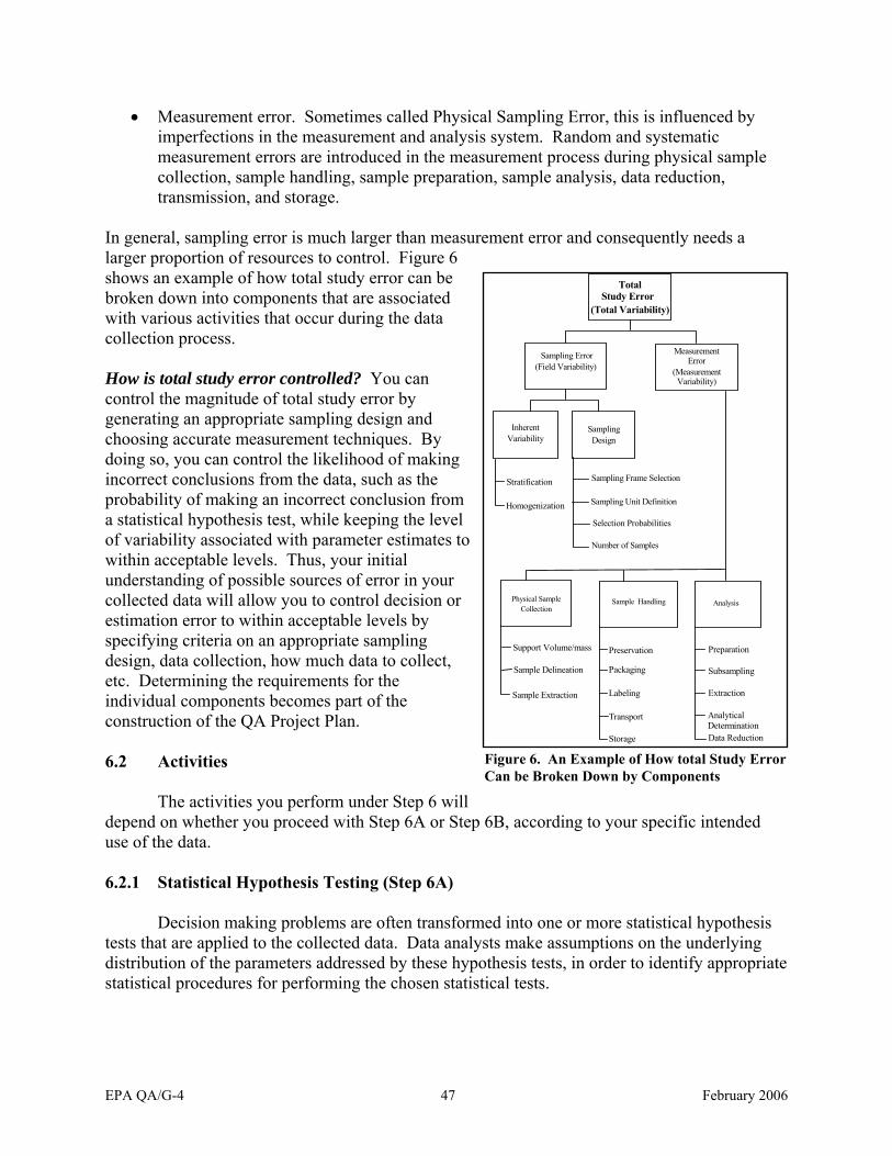
Total Study Error

(Total Variability)

Sampling Error (Field Variability)

Measurement Error

(Measurement Variability)

Inherent Variability

Sampling Design

Sampling Frame Selection

Sampling Unit Definition

Selection Probabilities

Number of Samples

Physical Sample Collection

Sample Handling Analysis

Support Volume/mass

Sample Delineation

Sample Extraction

Preservation

Packaging

Labeling

Transport

Storage

Preparation

Subsampling

Extraction

Analytical Determination Data Reduction

Stratification

Homogenization

• Measurement error. Sometimes called Physical Sampling Error, this is influenced by imperfections in the measurement and analysis system. Random and systematic measurement errors are introduced in the measurement process during physical sample collection, sample handling, sample preparation, sample analysis, data reduction, transmission, and storage.

In general, sampling error is much larger than measurement error and consequently needs a larger proportion of resources to control. Figure 6 shows an example of how total study error can be broken down into components that are associated with various activities that occur during the data collection process.

How is total study error controlled? You can control the magnitude of total study error by generating an appropriate sampling design and choosing accurate measurement techniques. By doing so, you can control the likelihood of making incorrect conclusions from the data, such as the probability of making an incorrect conclusion from a statistical hypothesis test, while keeping the level of variability associated with parameter estimates to within acceptable levels. Thus, your initial understanding of possible sources of error in your collected data will allow you to control decision or estimation error to within acceptable levels by specifying criteria on an appropriate sampling design, data collection, how much data to collect, etc. Determining the requirements for the individual components becomes part of the construction of the QA Project Plan.

6.2 Activities Figure 6. An Example of How total Study Error Can be Broken Down by Components

The activities you perform under Step 6 will depend on whether you proceed with Step 6A or Step 6B, according to your specific intended use of the data.

6.2.1 Statistical Hypothesis Testing (Step 6A)

Decision making problems are often transformed into one or more statistical hypothesis tests that are applied to the collected data. Data analysts make assumptions on the underlying distribution of the parameters addressed by these hypothesis tests, in order to identify appropriate statistical procedures for performing the chosen statistical tests.


How can statistical hypothesis testing lead me to make an incorrect conclusion or decision? Due to the inherent uncertainty associated with the collected data, the results of statistical hypothesis tests cannot tell you with certainty whether a given situation is true. You must be willing to accept some likelihood that the outcome of the test will lead you to make an erroneous conclusion, i.e. a decision error.

When a decision needs to be made, there are typically two possible outcomes: either a given situation is true, or it is not. We will never know which outcome is true in reality, but we collect data and perform a statistical hypothesis test on the data so that an informed decision could be made on which outcome is more likely to hold. In formulating the statistical hypothesis test, one of the two outcomes is labeled the baseline condition and is assumed to represent the de facto, true condition going into the test (for example, the permitting release level is being met). The other situation is labeled the alternative condition (for example, the permitting level is being exceeded). You retain the baseline condition until the information (data) from the sample indicates that it is highly unlikely to be true. Then, once a statistical test has been applied to the data, the outcome of this test will lead you to make a decision:

• There is insufficient evidence from the data to indicate that the baseline condition is false, and therefore, you conclude that the baseline condition remains true, or

• There is sufficient evidence from the data to indicate that the baseline condition is false beyond a reasonable doubt, and therefore, you conclude that the assumption that the baseline condition holds can be rejected in favor of the alternative condition being true.

• The standard presumption is in favor of the baseline condition and so carefully defining this baseline condition is important to the outcome of the decision process. Guidance is provided later in this section on selecting an appropriate baseline condition.

The statistical theory behind hypothesis testing allows you to quantify the probability of making decision errors given the data that you will collect. Therefore, by specifying the hypothesis testing procedures during the design phase of your project, you can also specify performance or acceptance criteria associated with your collected data that will lead to controlling the chance of making decision errors.

What types of decision errors could I make in a statistical hypothesis test? Table 7 illustrates that there are four possible outcomes of a statistical hypothesis test. These four outcomes are determined according to:

• Which condition is true in reality (i.e., last two columns of the table), and • Which of these two conditions you decide is true based on the outcome of the test applied

to your collected data (i.e., last two rows of the table).

Obviously, two of the four outcomes lead to no decision error: when the results of the test lead you to correctly adopt the true condition, whether it be the baseline or alternative condition. The remaining two outcomes (i.e., the shaded cells within Table 7) represent the two possible decision errors:


Table 7. Statistical Hypothesis Tests Lead to Four Possible Outcomes Decision You Make by Applying the

Statistical Hypothesis Test to the Collected Data

True Condition (Reality) Baseline Condition

is True Alternative Condition

is True Decide that the

Baseline Condition is True Correct Decision Decision Error (False Acceptance)

Decide that the Alternative Condition is True

Decision Error (False Rejection) Correct Decision

• A false rejection decision error occurs when your data lead you to decide that the baseline condition is false when, in reality, it is true.

• A false acceptance decision error occurs when your data are insufficient to change your belief that the baseline condition is true when, in reality, it is false.

The primary aim of Step 6A of the DQO Process is to arrive at upper limits on the probabilities of each of these two types of decision errors that you and the planning team find acceptable.

As an example, consider a regulatory situation in which the mean concentration of a contaminant in an effluent discharge should not exceed the permitted level. Your baseline condition would be that the true mean concentration of the effluent is less than or equal to the permitted level, while your alternative condition would be that the true mean exceeds the permitted level. If the baseline condition was actually correct, but your sample data happened to have a preponderance of high values which resulted in a high sample mean, the outcome of the statistical hypothesis test may lead you to conclude that the effluent exceeds the permitted level. Thus, your data would lead to rejecting the baseline condition in favor of the alternative condition, although in reality, the baseline condition was true. This is an example of making a false rejection decision error.

If a statistician is part of the team or is being consulted, a slightly different terminology is used. In the statistical language of hypothesis testing, the baseline condition is called the null hypothesis (Ho) and the alternative condition is called the alternative hypothesis (Ha). Statisticians interpret decision errors as follows:

• A false rejection decision error, or a Type I error, occurs when you reject the null hypothesis when it is actually true. The probability of this error occurring is called alpha (α) and is called the hypothesis test’s level of significance.

• A false acceptance decision error, or a Type II error, occurs when you fail to reject the null hypothesis when it is actually false. The probability that this error will occur is called beta (β).

• Frequently, a false rejection decision error is the more severe decision error, and therefore, criteria placed on an acceptable value of alpha (α) are typically more stringent than for beta (β).


• Statisticians call the probability of rejecting the null hypothesis when it is actually false (i.e., the bottom right corner of Table 7) the statistical power of the hypothesis test. Statistical power is a measure of how likely the collected data will allow you to make the correct conclusion that the alternative condition is true rather than the default baseline condition and is a key concept in determining DQOs for decision-making problems. Note that statistical power represents the probability of “true rejection” (i.e., the opposite of false acceptance) and, therefore, is equal to 1-β.

How can you control the probability of making decision errors? You can never totally eliminate the possibility that you will make a decision error from your data when performing a statistical hypothesis test. However, if you set criteria within your study design that control the largest components of total study error in your data, you will also be controlling the likelihood of making decision errors. For example, if you expect sampling design error to be a relatively large component of total study error, you can control the probability of making a decision error by collecting a larger number of samples or by developing a better sampling design (i.e., a better way of deciding where and when to sample). If the analytical component of the measurement error is believed to be relatively large, you can control the probability of making a decision error by analyzing multiple individual samples and then using the mean of these samples, or by using more precise analytical methods. In some instances, your planning team will actually be able to address both components of total error.

In some cases, it is unnecessary for the planning team to place very stringent controls on both types of decision errors (i.e., placing very small limits on the range of acceptable decision error probabilities) in order for the hypothesis test to yield a defensible decision. If the consequences associated with making one type of decision error are relatively minor, it may be possible to make a defensible decision despite collecting relatively imprecise data or a small amount of data. For example, in a particular hazardous site assessment, the site would be assumed hazardous unless data can demonstrate otherwise. The consequence of retaining the assumption that the site is hazardous when, in reality it is not, may be relatively minor under these circumstances. Specifying that only a moderate number of samples will be collected from the site, analyzed using a field screening analytical method, using only a limited number of confirmatory analyses could be satisfactory.

Conversely, if the consequences of making decision errors are severe (e.g., would lead to increasing the likelihood of adverse human health effects), you will want to develop a data collection design that exercises more control over sampling and measurement errors. For example, in a waste discharge investigation, deciding that a discharge is not hazardous when it truly is hazardous may have serious consequences because the discharge may pose a risk to human health and to the environment. Therefore, to the extent that you need to place very stringent limits on the probability of making this type of decision error, can lead to a large number of samples being collected and possibly the use very precise analytical methods.

The DQOs that you establish will specify requirements that the collected data will need to satisfy in order to ensure that the likelihood of making decision errors meet your needs. As you complete Steps 6 and 7 of the DQO Process, you will need to strike a balance between the


consequences of making decision errors and the costs that you will incur in collecting data that achieve the performance and acceptance criteria (data quality objectives) that you set. It may be necessary to iterate between Step 6 and Step 7 several times before this balance is achieved. This is not an easy part of the DQO Process. Rather than specifying arbitrary limits (e.g., “probability of a false rejection decision error will not exceed 0.05; probability of a false acceptance decision error will not exceed 0.20”), your planning team should fully explore balancing the risk of making incorrect decisions with the potential consequences associated with these risks. In the early stages of DQO development, it is recommended that a very stringent choice be made initially so that the planning team can investigate the resulting consequences of that choice during their activities under Step 7 of the DQO Process. As the process is iterated in arriving at an acceptable balance, the planning team gains the information they need to determine whether the requirements should be relaxed. Software that enables the planning team to investigate alternatives is discussed in Step 7 of the DQO Process.

When multiple decisions units exist and, therefore, multiple decisions are to be made, then the team needs to consider whether they want to limit the probability of making at least one incorrect decision (e.g., leaving at least one contaminated unit unremediated), rather than the probability of making an incorrect decision for a particular sampling unit. The probability of making at least one incorrect decision increases exponentially with the number of decisions to be made. In statistical language this is known as controlling the “experiment-wise” error rate, while controlling for the probability of making an incorrect decision for a particular unit corresponds to controlling the “comparison-wise” error rate. If multiple decisions are expected and the planning team wishes to control the experiment-wise error rate, then it is necessary to implement appropriate multiple comparison procedures within the statistical analysis of the data.

How do you express “quality” with regard to making a decision from a statistical hypothesis test? A graphical tool called a Decision Performance Curve is used to characterize the desired level of quality associated with applying a statistical hypothesis test to collected data in order to make a decision. Statisticians refer to this curve as an “operating characteristic curve” or a “power curve.” Figure 7 depicts two examples of a Decision Performance Curve when testing the null hypothesis that the true (unknown) value of a parameter falls below some Action Level (baseline condition) versus an alternative hypothesis that it exceeds the Action Level (alternative condition). The horizontal axis (x-axis) of Figure 7 lists the range of possible true values for the parameter (which includes the Action Level), while the vertical axis (y-axis) lists the range of probabilities (from 0 to 1) of deciding from the test that the true value of the parameter exceeds the Action Level (i.e., the alternative condition is true). Intuitively, when the true value of the parameter is very low, the chance any collected data will lead you to decide that the true value exceeds the Action Level will be low. This chance increases when the true value of the parameter becomes close to the Action Level.

If you had perfect knowledge of the true value of the parameter of interest (purely hypothetically) you would never make an incorrect decision. Therefore, for all values of the x-axis that fall at or below the Action Level (i.e., the baseline condition), the Decision Performance Curve would specify a probability of 0 (i.e., no possibility of rejecting this hypothesis). For all values of the x-axis that fall above the Action Level (i.e., the alternative condition), the Decision


Pro

babi

lity

ofD

ecid

ing

that

the

Par

amet

erE

xcee

dsth

eA

ctio

nL

evel

Usi

ngSa

mpl

edD

ata

Performance Curve would specify a probability of 1 (i.e., certain rejection). This scenario is represented by the “ideal” Decision Performance Curve in Figure 7. However, because you will

1

0.9

0.8

0.7

0.6

0.5

0.4

0.3

0.2

0.1

0

Low True Value of the Parameter High Action Level

Realistic Decision

Performance Curve

Ideal Decision

Performance Curve

Figure 7. Two Examples of Decision Performance Curves

perform this hypothesis test using collected data having inherent variability and uncertainty, the chance of rejecting this hypothesis will more realistically increase gradually from near 0 for true values far below the Action Level, to near 1 for true values far above the Action Level. This is represented by the “realistic” Decision Performance Curve in Figure 7. The shape and steepness of the Decision Performance Curve is a consequence of a number of factors, including the sample design, the precision associated with the collected data, and the number of samples taken.

As seen in the remaining discussion in this section, Step 6A of the DQO Process involves defining the baseline condition for your test and establishing tolerable limits on decision error probabilities at a few critical points along the x-axis of Figure 7 (i.e., possible true values of the parameter of interest). This will result in Decision Performance Goals which, when plotted, will approximate a Decision Performance Curve and specify your tolerable risks of making decision errors.

How do I define the baseline condition for my test? The baseline condition (i.e., null hypothesis) is assumed to hold unless convincing information from your collected data to make you reject it in favor of the alternative condition. Together, the baseline and alternative conditions cover the entire range of possible true values of the parameter being characterized (i.e., the x-axis in Figure 7). For this discussion, we will continue to use the term Action Level to represent the value in this range of possible true values that serves as the dividing line between the baseline and alternative conditions (this was determined in Step 5 of the DQO Process).


In certain instances, the baseline condition may be prescribed for you in regulations. For example, the baseline condition in RCRA facility ground water monitoring is that the concentration is within background levels (i.e. the true parameter value is below the action level). In the absence of regulatory considerations, the planning team should define the baseline condition by evaluating the potential consequences of making decision errors based on the outcome of the statistical hypothesis test, and as a result, taking the wrong actions. For example, incorrectly accepting a baseline condition that remediation of a contaminated site is unnecessary could result in adverse health effects from the continued exposure, and a loss of integrity if the error is later discovered. In contrast, incorrectly concluding that this baseline condition be rejected could lead to unnecessary remediation costs and a diversion of resources from more urgent problem areas. You need to determine which of these two types of decision errors has the more severe consequences, especially when the true value of the parameter is near the Action Level. For example, if false rejection is the more severe decision error, then you would define the baseline condition to represent a range of possible true values for the parameter for which the probability of a false rejection is likely to be low. Finally, defining the baseline condition can be done, in part, based on prior knowledge. For example, you may have good cause to believe that the true value for the parameter is above some specified level, and therefore, you define the baseline condition to correspond to this situation and require your data to demonstrate otherwise.

What is a “gray region,” and how does it enter into determining data quality criteria? Within the possible values that makes up the alternative condition is a set of values that start at the Action Level and extends to the left or right of the Action Level depending on the choice of baseline condition; it is called the gray region. This region is really where it is “too close to call”, where the consequences of making a decision error are relatively minor. The gray region is illustrated by shaded areas within Figures 8 and 9, which represent the following two scenarios:

Figure 8: When the alternative condition represents all possible parameter values above an Action Level:

• H0: the parameter is equal to or less than the Action Level • HA: the parameter exceeds the Action Level

Figure 9: When the alternative condition represents all possible parameter values below an Action Level:

• H0: the parameter equal to or exceeds the Action Level • HA: the parameter is less than the Action Level

Note that while Figures 8 and 9 appear to look similar, the gray region has switched depending on how the baseline condition is defined:


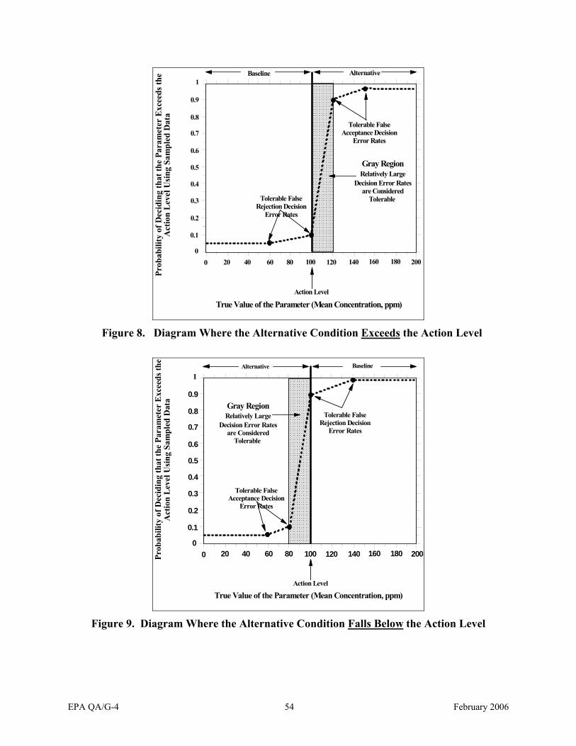
True Value of the Parameter (Mean Concentration, ppm)

Alternative 1

0.9

0.8

0.7

0.6

0.5

0.4

0.3

0.2

0.1

0 0 20 40 60 80 100 120 140 160 180 200

Action Level

Baseline

Gray Region Relatively Large

Decision Error Rates are Considered

Tolerable Tolerable False Rejection Decision

Error Rates

Tolerable False Acceptance Decision

Error Rates

Prob

abili

ty o

f Dec

idin

g th

at th

e Pa

ram

eter

Exc

eeds

the

Act

ion

Lev

el U

sing

Sam

pled

Dat

a

Figure 8. Diagram Where the Alternative Condition Exceeds the Action Level

Alternative

1

0.9

0.8

0.7

0.6

0.5

0.4

0.3

0.2

0.1

0 0 20 40 60 80 100 120 140 160 180 200

Action Level

True Value of the Parameter (Mean Concentration, ppm)

Baseline


Decision Error Rates are Considered

Tolerable

Tolerable False Acceptance Decision

Error Rates

Tolerable False Rejection Decision

Error Rates

Prob

abili

ty o

f Dec

idin

g th

at th

e Pa

ram

eter

Exc

eeds

the

Act

ion

Lev

el U

sing

Sam

pled

Dat

a

Figure 9. Diagram Where the Alternative Condition Falls Below the Action Level


• In Figure 8, the baseline condition corresponds to possible values of the parameter that fall below the Action Level. Therefore, the curve in this figure represents the probability of rejecting Ho for HA. Thus, portions of the curve falling to the left of the Action Level represent the probability of making a false rejection error (α), while portions of the curve falling to the right of the Action Level represent the false acceptance error (β) [reading from the top down].

• In Figure 9, the baseline condition corresponds to possible values of the parameter that fall above the Action Level. Therefore, the curve in this figure represents the probability of failing to reject Ho for HA. Thus, portions of the curve falling to the left of the Action Level represent the probability of making a false acceptance error, while portions of the curve falling to the right of the Action Level represent the false rejection error (α) [reading from the top down].

If you had perfect information from which to make a decision, you would reject the assumption that the baseline condition was true whenever the true value of the parameter was within the gray region. However, because you won’t have perfect information, Figures 8 and 9 suggest that the probability of rejecting the assumption that the baseline condition was true can be relatively small at values within the gray region that are close to the Action Level. This would imply a large probability of a false acceptance decision error. This happens because you want to control the probability of a false rejection decision error within the range of possible parameter values that fall within the baseline condition. The high likelihood of making a false acceptance error within this region, and your recognition and acceptance of this high likelihood, is what gives the “gray region” its name.

The gray region is bounded on one side by the Action Level and the other by that value where the consequences of making a false acceptance decision error becomes serious, i.e. the consequences of committing a false acceptance decision error would be significant. In general, the narrower the gray region, the greater the number of samples you will need in order to achieve the criteria you’ve placed on the false acceptance decision error probability, because the area in which high false acceptance error probabilities are considered tolerable is reduced. In statistical hypothesis testing language, the width of the gray region is called the minimum detectable difference and is often expressed as the Greek letter delta (Δ). This value is an essential part of the calculations that statisticians use to determine the number of samples that need to be collected so that you will have your stated confidence in decisions made based on the data collected.

It should be emphasized that the curves plotted in Figures 9 and 10 are graphical portrayals of Decision Performance Goals that are established during a study’s planning phase prior to formulating a sampling design. More discussion regarding the use and interpretation of these figures is given at the end of this section.

What if I determine that I don’t need to specify a gray region for my problem? In some situations, you may be making a decision from collected data without controlling one or both types of decision errors. In particular, if you are not controlling for false acceptance decision


errors, you are not specifying a gray region for your test. Consider the following two situations that may not lead to specifying a gray region:

• Some regulations require that an upper confidence bound on the value of a decision parameter (i.e., the largest value which the parameter can hold with a specified level of confidence) be compared to an Action Level. While this approach will control the probability of making a false rejection decision error, it does not control against making false acceptance decision errors.

• You may wish to use your data to make a yes/no decision simply by comparing a calculated mean value to some Action Level, without considering the variability associated with the calculated mean. In this situation, you are not performing a statistical hypothesis test and, therefore, are not specifying limits on making a wrong decision.

In both of these situations, you should specify as many Decision Performance Goals as your problem requires (e.g., control for false rejection decision errors such as in the first of these two situations). Then, you should design a plan for generating data that attempts to generate a decision performance curve (Figure 7) that achieves the Decision Performance Goals that you may have specified, plus is as steep as possible given your constraints on available resources. This will help keep false acceptance error probabilities low, although you may not necessarily have specified tolerable limits on these probabilities for possible parameter values that represent the alternative condition.

How do you establish tolerable limits on decision error probabilities? At one possible value of the parameter of interest, a decision error limit is the maximum probability that you are willing to tolerate of a decision error occurring, given that the true value of the parameter equals that particular value. By establishing decision error limits, you are expressing your tolerance for uncertainty and the risk you are willing to assume for making an incorrect decision.

At a minimum, there are two decision error limits you should specify:

• A false rejection decision error limit at the Action Level (which represents one boundary of the gray region)

• A false acceptance decision error limit at a point that will represent the other boundary of the gray region.

You set stringent decision error limits (i.e., low limits) when severe consequences (such as extreme risks to human health) would result from a particular decision error, and less stringent limits when moderate consequences would result. In general, the consequences of making a decision error become more severe as you consider possible values of the parameter that are farther away from the Action Level, and decision error limits should decrease as a result.

The most stringent decision error limits for environmental data are typically 0.01 (1%) for both false rejection and false acceptance decision errors. Therefore, this guidance recommends using 0.01 as the starting point for setting both false acceptance and false rejection decision error limits. If your planning team determines that the consequences of making a


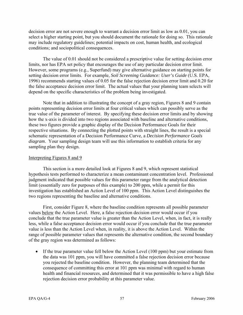
decision error are not severe enough to warrant a decision error limit as low as 0.01, you can select a higher starting point, but you should document the rationale for doing so. This rationale may include regulatory guidelines; potential impacts on cost, human health, and ecological conditions; and sociopolitical consequences.

The value of 0.01 should not be considered a prescriptive value for setting decision error limits, nor has EPA set policy that encourages the use of any particular decision error limit. However, some programs (e.g., Superfund) may give alternative guidance on starting points for setting decision error limits. For example, Soil Screening Guidance: User’s Guide (U.S. EPA, 1996) recommends starting values of 0.05 for the false rejection decision error limit and 0.20 for the false acceptance decision error limit. The actual values that your planning team selects will depend on the specific characteristics of the problem being investigated.

Note that in addition to illustrating the concept of a gray region, Figures 8 and 9 contain points representing decision error limits at four critical values which can possibly serve as the true value of the parameter of interest. By specifying these decision error limits and by showing how the x-axis is divided into two regions associated with baseline and alternative conditions, these two figures provide a graphic display of the Decision Performance Goals for their respective situations. By connecting the plotted points with straight lines, the result is a special schematic representation of a Decision Performance Curve, a Decision Performance Goals diagram. Your sampling design team will use this information to establish criteria for any sampling plan they design.

Interpreting Figures 8 and 9

This section is a more detailed look at Figures 8 and 9, which represent statistical hypothesis tests performed to characterize a mean contaminant concentration level. Professional judgment indicated that possible values for this parameter range from the analytical detection limit (essentially zero for purposes of this example) to 200 ppm, while a permit for this investigation has established an Action Level of 100 ppm. This Action Level distinguishes the two regions representing the baseline and alternative conditions.

First, consider Figure 8, where the baseline condition represents all possible parameter values below the Action Level. Here, a false rejection decision error would occur if you conclude that the true parameter value is greater than the Action Level, when, in fact, it is really less, while a false acceptance decision error would occur if you conclude that the true parameter value is less than the Action Level when, in reality, it is above the Action Level. Within the range of possible parameter values that represents the alternative condition, the second boundary of the gray region was determined as follows:

• If the true parameter value fell below the Action Level (100 ppm) but your estimate from the data was 101 ppm, you will have committed a false rejection decision error because you rejected the baseline condition. However, the planning team determined that the consequence of committing this error at 101 ppm was minimal with regard to human health and financial resources, and determined that it was permissible to have a high false rejection decision error probability at this parameter value.


• In considering other possible true values of the parameter within the alternative region, the planning team determined that the false acceptance decision error probability did not need to be controlled at values below 120 ppm. However, making a false acceptance decision error at 120 ppm would result in an elevated risk of adverse health effects. Therefore, the planning team specified 120 ppm as the first value at which the probability of a false acceptance decision error needs to be controlled. As a result, it was taken to equal the second boundary of the gray region.

Upon determining the gray region, the planning team then evaluated possible decision error limits at various true values of the parameter, balancing the consequences of making these decision errors with the resources required to achieve the decision error limits that they would set. They agreed to place a limit of 0.10 (10%) on the probability of making a false acceptance decision error at 120 ppm (This would correspond to a 90% chance of correctly rejecting the baseline assumption at 120 ppm). The planning team also determined that the probability of making a false acceptance decision error at 160 ppm should be no more than 0.05 (5%), due to the heightened risk of adverse health effects at this level. In a similar manner, the planning team determined that if the true parameter value was at the Action Level (100 ppm), the probability of making a false rejection decision error should be no more than 0.10 (10%), and at 60 ppm, this probability should be no more than 0.05 (5%). A Decision Performance Goal diagram results by connecting the four points on this graph.

Consider Figure 9, where the baseline condition represents all possible parameter values above the Action Level. The Decision Performance Goal diagram looks very similar to that of Figure 8, except that the regions representing baseline and alternative conditions have switched, and therefore, the gray region is on the other side of the Action Level. Figure 9 shows that at the Action Level, the planning team will tolerate a 10% chance of making a false rejection decision error, while the false rejection decision error limit decreases to 0.01 (1%) if the true value of the parameter equaled 140 ppm. At the edge of the specified gray region, 80 ppm, the planning team is willing to tolerate a 10% risk of making a false acceptance decision error, while this decision error limit reduces to 5% if the true value of the parameter is 60 ppm.

6.2.2 Estimation (Step 6B)

The inherent variability and uncertainty in your collected data indicates there will be uncertainty associated with your estimate. The extent of uncertainty needs to be reported along with the actual estimate itself. By designing the data collection process appropriately you can control the level of uncertainty in your parameter estimates to achieve criteria that you and your planning team find acceptable.

The bias and precision associated with your collected data directly impact the level of uncertainty in parameter estimates. Bias and precision (collectively known as accuracy) are two principal attributes, or characteristics, of data quality in environmental studies. Bias represents systematic error (i.e., persistent distortion that causes constant errors in a particular direction), while precision represents random error (i.e., error among repeated measures of the same property under identical conditions, but not systematically in the same direction or of the same


magnitude). As part of the DQO Process, you should ensure that information on bias and precision are documented in the QA Project Plan.

What are some examples of estimates commonly calculated for environmental studies? Typically, managers are interested in estimating “average” conditions and/or “extreme” conditions. Selecting a summary statistic to represent the condition of interest to the sponsor of an investigation is an important first step in planning an environmental study and is in many respects equivalent to establishing a decision rule for a decision-oriented study. The choice of statistic should take into consideration the underlying shape of the distribution from which the samples were taken. If the distribution is skewed, the mean would be a poor estimate of the average condition, and instead a median would be more appropriate. Transforming data sets, for example a log-transformation, may be useful in some cases, but estimates on transformed data are often very difficult to interpret. Finally, it also is important to have some measure of uncertainty or precision for the selected estimate in mind, so that during the planning phase of the data collection effort it is possible to express desired levels of certainty, and the design (type, number and quality of measurements) can be targeted at achieving the expressed criteria. Confidence intervals and other uncertainty indicators can be established around point estimates as well as around slopes, ratios and even contours (e.g., isopleths).

Examples of real-world estimates for which data are frequently collected:

• Means or medians to characterize the “average” characteristic of a population; • Upper percentile, upper confidence limit (UCL) or upper tolerance limit to

characterize the extreme values in a population; • Exposure point concentrations used in risk assessments as a conservative estimate of

central tendency (for example, 95% UCL on the mean); • Bivariate relationships such as slopes or ratios that can be used in modeling (for

example, to model transfer of contaminants between an environmental media such as soil, sediment or water to tissue of exposed organisms);

• Estimates of total study variance for use in designing follow-on data collection efforts or refining monitoring programs;

• Estimates of measurement bias and precision and associated minimum detection limits or quantitation limits for use in determining how well a measurement method performs for a specific range of concentrations;

• Rates of processes such as flow rates, rates of biologically mediated transport of contaminated soil or sediment, rates of contaminated water movement through the vadose zone, evaporation rates, environmental half-life, or temporal trend lines;

• Estimates of toxicity or Toxicity Reference Values; • Spatial contours representing the location and area predicted to be at or above some

concentration of interest; • Population size, recruitment rate, total biomass, rates of primary or secondary

productivity; • Proportions, such as the proportion of time a measurement exceeds a threshold.

In what ways can I express uncertainty in a parameter estimate? You will most often express uncertainty in a parameter estimate in one of two ways:


• As a standard error, reported either in absolute or relative terms (but not easy to interpret).

• By expanding the single point estimate to cover an interval of possible values (a confidence interval or confidence limit, a tolerance interval or tolerance limit, or a prediction interval or prediction limit, which are easier to interpret).

By choosing a method for expressing uncertainty, you are specifying a performance metric that quantifies uncertainty and, therefore, allows you to establish limits against which this quantity can be compared. Similar to statistical hypothesis testing, levels of uncertainty that you find tolerable will be derived by considering the potential consequences associated with high levels of uncertainty and balancing this with available resources and other constraints that you may encounter.

Standard Errors

The standard error calculation frequently depends on factors that include the amount of data available, the underlying distribution, and the variability in the data used to calculate the parameter estimate. A standard error can be expressed in either absolute form (i.e., a single number that accompanies the estimate) or relative to the value of the parameter estimate (i.e., a proportion or percentage of the estimate). When the standard error is expressed in relative terms, you are able to more easily specify criteria on the size of the standard error. For example, you can specify a goal that the standard error will not exceed 30% of the value of the parameter estimate. As you can achieve this goal only by collecting a sufficient amount of data that achieve a certain degree of precision, this requirement would contribute to the performance or acceptance criteria that you establish for the collected data.

An example of performance or acceptance criteria placed on the data for controlling the magnitude of a standard error:

• A sufficient amount of data will be collected to ensure that the standard error associated with the estimated mean concentration is no higher than 40% of the mean estimate.

Statistical Intervals

Often decisions have to be made from a limited amount of sample data. For example, the property owners need to assess lead concentrations in soil before converting the site to a residential community. Six random sample data values can be described by a “point estimate” that provides a concise summary of the sample results. A statement such as “The average lead concentration for the 6 sediment samples was 2.3 ug/g” gives an overview of lead concentrations in those 6 samples but does not provide any information about the precision of the estimate. It is unlikely that lead concentrations on the site are 2.3 ug/g; however, we would expect lead concentrations to be somewhat close to that value.


One way to quantify uncertainty is to construct a statistical interval around a point estimate. There are a variety of statistical intervals that can be constructed from sample data. The appropriate interval depends on the specific application. Three of the most frequently used intervals are confidence intervals, tolerance intervals and prediction intervals.

Which statistical interval should I use? First it is important to consider whether your main interest is in describing the population from which the sample has been taken, or in predicting the results of a future sample from the same population. Intervals that describe a population include confidence intervals for the population mean or population standard deviation. Tolerance intervals contain a particular portion of the population with a specified probability. Prediction intervals, on the other hand, can be for a future single value, a future mean or future standard deviation.

Confidence Intervals

A confidence interval is an interval used to estimate a population parameter from sample data. It is generally composed of two parts, an interval calculated from the data and a confidence level associated with the interval. The confidence interval is generally of the form: point estimate ± margin of error (read as “estimate plus or minus margin of error”). The point estimate is a single value computed from the sample data. To account for the possibility of estimation error, the margin of error is included in the confidence interval to provide a range of possible parameter values. The margin of error is what determines the width of the confidence interval.

In addition to the confidence interval, there is a confidence level associated with the interval. A confidence level gives the probability that the interval will capture the population parameter in repeated sampling. Therefore, you can infer that you have a certain level of confidence that the interval contains the true value of the parameter. In other words, you are stating how confident you are in the process that produces the interval. The level of confidence is expressed in terms of a percentage, e.g., 95% confidence. The larger the percentage, the more confident you are that the interval contains the true value of the parameter. Consequently, the higher the confidence level, the wider the interval. Thus there is a trade-off between how confident you are and how wide your interval will be.

One of the most common confidence intervals constructed is a confidence interval to contain the population mean. Confidence intervals can, however, be constructed for any population parameter of interest.

How are confidence intervals for the population mean constructed? A sample mean is calculated and used as the estimate around which the interval is constructed. The margin of error used to construct the interval depends on the assumption that was made about the population distribution and the sample standard deviation.

Confidence intervals for the population mean are easy to construct and easy to understand. However, as with the construction of any statistical interval, the interval is strongly affected by outliers. Fortunately, the procedures are robust with respect to deviations from the


assumption of normality when there are no outliers, especially when the population distribution is roughly symmetric.

What is the difference between a two-sided confidence interval and a one-sided confidence bound? A two-sided confidence interval has both an upper and a lower bound usually constructed to have an equal amount of uncertainty associated with the population parameter outside each of the two endpoints. Two-sided confidence intervals are used when you wish to create a closed interval that will bracket the population parameter with a certain amount of confidence. For example, you might construct a two-sided interval to contain the true mean relative risk for your site, this interval states with a certain amount of confidence that the true mean relative risk lies in a range between these two values. The one-sided confidence bound, or one-sided confidence limit, is restricted to either the upper or the lower bound of the two-sided confidence interval depending on the situation. In environmental applications, it is often the upper limit that is of interest. For example, the upper confidence limit (UCL) for mean concentrations in soils can be used for baseline screening assessments. The lower confidence limit is used in a similar manner for biological studies (e.g., longevity of organisms exposed to contamination) and other types of environmental assessments.

What if my assumptions for constructing confidence intervals are not met? The assumption of random sampling is critical for any type of statistical interval you are constructing. Statistical intervals incorporate only the randomness inherent in the sampling process, they do not take into account any bias that may be introduced by non-random sampling. Thus departures from this assumption may lead to a false sense of security regarding the usefulness of your interval.

Confidence intervals for the population mean are fairly insensitive to deviations from normality, unless the sample size is very small and/or the deviation from normality is extreme. Thus a confidence interval for the mean can be constructed for most practical situations even if the assumption of normality is not strictly met. The resulting confidence interval, however, is approximate rather than exact.

What if my data are clearly non-normal or my sample size is so small that tests of normality are not appropriate for my data? For these cases, non-parametric or “distribution-free” alternatives for constructing confidence intervals for the population mean are available. Nonparametric tests make few or no assumptions about the distribution of the sample data, and do not rely on distribution parameters in the construction of statistical intervals. Thus their chief advantage is improved reliability when the underlying population distribution is unknown. There is at least one nonparametric equivalent for each parametric (i.e., distributional assumptions are made) type of statistical interval.

There are some limitations to constructing statistical intervals using nonparametric methods. In general it is not possible to obtain a nonparametric interval with precisely the desired associated confidence level as a parametric interval for the same population parameter. Another weakness of nonparametric intervals is that they can be much wider than distribution dependant ones. Relatively large sample sizes are needed to reduce the width of a nonparametrically constructed interval.


While “distribution free” or nonparametric intervals have some limitations, they still deserve consideration. By their very nature, they are free from the assumptions that restrict other construction methods. Also remember that constructing parametric intervals when their underlying assumptions are violated can lead to incorrect intervals.

How are hypothesis tests and confidence intervals related? Hypothesis tests and confidence intervals are two sides of the same coin. Often a confidence interval can be used to test a hypothesis rather than performing the entire hypothesis test itself. For example, suppose a one-sided 95% upper confidence limit for the true mean is calculated and this value exceeds the hypothesized mean. We would conclude that we can not reject the null hypothesis for these data. Thus a one-sided 95% upper confidence limit gives the same “accept” or “reject” information that a one-sided hypothesis test at a 0.05 significance level. There is a similar relationship between a two-sided 95% confidence interval and a two-sided hypothesis test at a 0.05 significance level.

What does the planning team need to know to determine an acceptable level of precision in the confidence interval? Typically, criteria for this type of study are defined by the need to estimate the unknown parameter to within a specified amount with a given confidence level. In doing this, the planning team is placing specifications on the maximum width of the confidence interval (or on the margin of error, or half-width).

The width of a confidence interval will generally depend on:

• The amount of data used to calculate the interval, and • The precision, or variability, of these data.

Therefore, in placing limits on the maximum width of the confidence interval, you are specifying criteria on the precision and the amount of data needed to calculate this interval.

Is it possible to control the width of a confidence interval? The width of the confidence interval for the mean is directly related to the margin of error used to calculate the interval, the larger the margin of error, the larger the width of the confidence interval. There are three ways to reduce the width of the confidence interval: reduce the variability, increase the sample size, or reduce the confidence level. Practically speaking, it is not usually possible to reduce the variability in your data, thus the most common way to reduce the width of the confidence interval is to increase the number of samples collected.

The remaining factor that affects the width of a confidence interval is the level of confidence that you associate with the interval. As the level of confidence increases, the size of the interval increases. For example, a 95% confidence interval will be wider than a 90% confidence interval in order to support your claim of having 5% more confidence that the interval contains the true value of the population parameter.

What is the difference between a confidence interval and a confidence limit? A confidence interval is a range of values constructed around the estimate of interest that includes the variability in the data and the variability in the estimate. The interval has a lower bound and an


upper bound. The upper bound is referred to as the Upper Confidence Limit or UCL, while the lower bound is known as the Lower Confidence Limit, or LCL. UCLs are used in a variety of environmental applications. For example, the UCL of the population mean is used in risk assessment as a conservative estimate of the average exposure.

How do I interpret the resulting confidence interval? Confidence intervals are often misinterpreted. There is an overwhelming desire to interpret the confidence level (i.e. 95%, 99%) associated with the interval as “the chance that the statistic will fall into that interval.” This is not how the interval should be interpreted.

The goal of the confidence interval is to make inferences about the population parameter with a certain level of confidence. Thus the interpretation of the confidence interval should include a statement about the population parameter of interest and the amount of confidence we have in the interval we have created.

The confidence level associated with the interval is a reflection of our confidence in the statistical process used to create the confidence interval. Confidence intervals are based on randomly collected sample data that, by their nature, are subject to sampling variation. As a result of that variation, the calculated interval will sometimes not contain the parameter of interest it was calculated to contain. Thus, statistical intervals are only correct a certain percentage of the time, this percentage is defined by the confidence level.

We can never know if the population parameter truly falls within the interval we calculate. In fact, the population parameter is an unknown fixed quantity that is either in the interval or not. All we can say about the population parameter is that if, for example, we were to calculate one hundred 95% confidence intervals (each to contain the population parameter of interest from different random samples) 95 of those intervals will contain the population parameter while the other 5 will not. We hope that the interval we calculated is one of those 95.

What does the planning team need to consider in determining level of confidence? The degree of confidence to be placed in a confidence interval should be determined according to the importance of ensuring that the interval contains the true value of the parameter for a specified width. Confidence intervals of 90% to 99% are the most common intervals encountered in the scientific literature, with 95% confidence intervals being most common. For studies requiring that the calculated interval contain the true parameter value with a very high level of confidence (e.g., estimating the mean concentration of a compound that yields highly adverse health effects in sensitive subpopulations), a 99% or 99.9% confidence level may be necessary. In contrast, for studies that require only a moderate degree of confidence, such as a screening study, a 90% or even lower confidence interval may be acceptable.

Note that when important statistical assumptions are not satisfied, the actual confidence level associated with the interval you calculate may be considerably lower than the confidence level you have prescribed.


Tolerance Intervals

Tolerance intervals are similar to confidence intervals in that they portray uncertainty in a population parameter; however with tolerance intervals the parameter is a specified proportion of the population distribution. Specifically, tolerance intervals estimate the range that should contain a certain percentage of the values in the population. Similar to the concept of confidence level, we cannot be 100% confident that that interval will contain the specified proportion, only a certain percentage. There are two different inputs associated with the tolerance interval: a degree of confidence and a percent coverage. For example, we may be 95% confident that 90% of the population will fall within the range specified by the tolerance interval.

In practice the entire tolerance interval is rarely used, rather the upper limit of the tolerance interval is often of interest in environmental applications. Upper Tolerance Limits (UTLs) are frequently recommended to characterize the upper tail of a distribution. A percentile is chosen and a confidence interval is constructed around that value. A percentile is defined as a value on a scale of one hundred that indicates the percent of a distribution that is equal to or less than it. For example, if a set of data is put in order, the 30th percentile is the piece of data that comes 30% of the way through the ordered data set. When attempting to characterize the upper tail of a distribution, a large percentile is chosen, 95th or 99th, and a confidence interval with a high confidence level, say 95%, is constructed about that percentile. The upper limit of this interval is then used in various environmental contexts, for example as performance criterion. Upper tolerance limits constructed in this way provide a conservative estimate that approaches, or sometimes exceeds, the maximum observed value.

How are upper tolerance limits used in environmental situations? UTLs are useful for establishing simple benchmarks representing ambient or background concentrations. Upper tolerance limits can be calculated for long term monitoring data from specific geographical areas of interest such as large estuaries, Great Lakes, or regional soils. A more detailed example:

A long-term sampling program has been underway to monitor the sediment and water quality across a large estuary called Moon Bay. Sampling stations were set up at over 50 locations across the bay, and monitored on a yearly basis. Recent efforts to evaluate total loading of contaminants to the Bay have pointed to a number of industrial and Federal sites that are suspected to be point sources for a number of contaminants including heavy metals, PCBs, Total PAH, and pesticides. Moon Bay scientists decided to evaluate data collected over the last 5 years to calculate a number of summary statistics that could shed light on how concentrations vary by looking at different subsets of stations. Of particular interest were estimates representing background or ambient conditions.

Managers requested that in addition to calculating estimates of central tendency (mean and median), a value representing the upper tail of the distribution, or extreme values also be estimated. After discussion with data analysts, the maximum observation was dismissed, since there was no way to characterize the uncertainty around this value. Instead, the upper 95th

percentile was chosen. To provide 95% confidence that the reported 95th percentile was not under estimated, the data analysts proposed to calculate an upper tolerance limit or UTL based on this value. This UTL was used as a screening threshold to determine which constituents were


present at levels in excess of the ambient data. While not a statistical test, this comparison was useful in identifying constituents that warranted further study.

Another area where tolerance intervals are useful is in ground-water data analysis. In many situations it is important to ensure that only a small fraction of compliance well sample measurements exceed a set limit to be protective of human health and the environment. By design, the tolerance interval is often constructed to cover all but a very small portion of the population, e.g. 90% confident that 99% of the population is contained in the interval. Thus you can evaluate how many extreme measurements are being sampled from compliance wells by comparing each compliance well measurement to the upper tolerance limit.

Finally, tolerance intervals are often used in monitoring for potential contamination. Compliance point samples are assumed to be similar to background values until evidence of contamination can be shown. One way to evaluate this assumption is to calculate an upper tolerance limit on background data and compare compliance point samples to that limit. If any of the compliance point samples exceed the upper tolerance limit, the well from which that sample was taken is deemed to have evidence of contamination.

What are the assumptions needed to compute tolerance intervals? The most critical assumption made when constructing tolerance intervals is that the data used for constructing the interval are representative of the population of interest and are a randomly collected sample. To ensure that the uncertainty in the estimate is attributable to random processes rather than systematic bias, data collected using a sample design based on randomization is critical. If this assumption is violated, tolerance intervals constructed from such data are of little practical use.

The adherence to the assumption of normality is more important for tolerance intervals than for other statistical intervals. Since tolerance intervals tend to concern the tails of the distribution, this is where deviations from normality are more pronounced. Tolerance intervals can be completely erroneous when the true underlying distribution is not normal. This is especially true for intervals that are constructed with a high degree of confidence and cover a large percent of the population. If the assumption of normality cannot be met, then one can construct nonparametric or “distribution free” tolerance intervals instead.

Prediction Intervals

While confidence and tolerance intervals estimate present population characteristics, the prediction interval estimates what future values will be, based upon previously collected data. Just as with confidence and tolerance intervals, prediction intervals incorporate the idea of a confidence level when attempting to determine what future values will be. For example, we may attempt to predict that the next set of samples will fall within a determined range with 99% confidence. To calculate prediction limits, we first must have estimates of the current population mean and standard deviation. We must also decide how many sampling periods and how many samples will be collected per sampling period. Once these factors are determined, we can calculate an interval for estimating those future observations. Prediction intervals are always larger than confidence intervals.


How are prediction intervals used in environmental situations? Groundwater monitoring is one area where prediction intervals are used to predict future measurements based on previously collected samples. Regardless of the type of samples available, either repeated measurements from a single well or multiple measurements on many wells, it is often of concern to calculate an interval that will contain either the next future measurement or all future measurements with a given level of confidence. The distinction between an interval for the next future measurement and the next several future measurements is crucial. For example, assume that monitoring data is collected quarterly and that during the next event lead measurements will be collected from a compliance well located downgradient of the facility. Based on data previously collected, it would be nice to calculate an interval that would contain the next single lead measurement with 95% confidence. This interval takes into consideration both the uncertainty in our estimates from our data and the uncertainty associated with the next single future value.

Often it is not the prediction interval that is of interest; rather it is the upper limit for the new measurement that is of concern. For example, lead concentrations that are low do not pose an environmental threat. Thus by providing an upper limit for the next future measurement, you are stating with a certain level of confidence that the next measurement will not exceed this upper prediction limit. Of course it is not often that a single future observation requires evaluating, more often it is a series of wells that will be sampled and evaluated together. An upper prediction limit can be calculated simultaneously evaluating lead measurements from a series of wells. In this case, the upper limit will be larger since it needs to state with a certain level of confidence that the next series of measurements will not exceed this upper limit.

What are the assumptions associated with prediction intervals? As with confidence and tolerance intervals, the assumption that the sample data is collected using a sample design based on randomization is critical. Data collected using convenience or judgmental sampling introduces bias into the data that is not accounted for when constructing prediction intervals. Another assumption for constructing prediction intervals is the assumption of normality. Fortunately, prediction intervals are relatively insensitive to deviations from normality unless the future sample size is very small or the deviation from normality is extreme. For this reason, prediction intervals for the single future event may be incorrect when the assumption of normality is not met. If the assumption of normality is violated there are non-parametric or “distribution free” prediction intervals that can be constructed.

6.3 Outputs

The primary output from Step 6 of the DQO Process is a set of performance or acceptance criteria (i.e., data quality objectives) that your collected data should achieve in order to minimize the possibility of either making a decision error or failing to keep uncertainty in estimates to within acceptable levels. You establish these criteria according to whether your problem is a decision-making problem requiring statistical hypothesis testing (Step 6A) or primarily an estimation problem (Step 6B).

In a statistical hypothesis setting, the outputs from performing Step 6A of the DQO Process that lead to performance or acceptance criteria on your collected data would include:


• Specification of the range of possible true values of the parameter of interest thatcorrespond to the baseline condition.

• Specification of the gray region containing possible true values of the parameter of interest that fall within the alternative condition and for which you can tolerate high probabilities of making false acceptance decision errors.

• The set of tolerable decision error limits at selected true values of the parameter of interest (i.e., at the boundaries of the gray region).

You generate these outputs by considering the consequences of making decision errors along the range of possible true values of the parameter of interest: false rejection decision errors within the range representing the baseline condition, and false acceptance decision errors within the range representing the alternative condition. Presenting these outputs with a Decision Performance Goal Diagram is an effective, graphical means of communicating, to the planning team and to stakeholders, draft versions of these outputs while they are being formulated, and as the final set of outputs.

When you will be calculating confidence intervals in an estimation setting, the outputs from performing Step 6B of the DQO Process are:

• The confidence level that specifies the likelihood that the interval will contain the true value of the parameter

• An acceptable width associated with the interval, expressed in either absolute or relative terms.

If you simply plan to calculate standard errors associated with your estimates, your outputs from Step 6B may correspond to bounds placed on the size of the standard error relative to the parameter estimate, either in absolute and relative terms, along with specifications placed on the various components of total study error in your data.

6.4 Example

For the two examples, the procedures of Step 6A (decision-making) were applied to Example 1, while the procedures of Step 6B (estimation) were applied to Examples 2, 3 and 4.


Setting baseline and alternative conditions. The planning team determined that any decision on the disposal route of a given container of waste fly ash must be made with the safeguard of the public’s health being of paramount importance. Following EPA Test Methods for Evaluating Solid Waste Physical/Chemical Methods SW 846, the collected data from a given container must demonstrate that the waste fly ash within that container is, in fact, nonhazardous to human health. To meet this requirement, the baseline condition has been established as "the waste is hazardous" (i.e., is at or above the Action


Level of 1.0 mg/L), while the alternative condition is “the waste is nonhazardous” (i.e., is below 1.0 mg/L). The statistical hypotheses are then:

Ho: true mean cadmium concentration in TCLP leachate is at or above 1.0 mg/L

Ha: true mean cadmium concentration in TCLP leachate is below 1.0 mg/L.

Unless there is conclusive information from the collected data to reject the null hypothesis (i.e., Ho, the baseline condition) for the alternative hypothesis (i.e., Ha, the alternative condition), we therefore assume that the baseline condition is true.

Determining the impact of decision errors. Recall that a “false acceptance decision error” corresponds to deciding that the waste fly ash is hazardous (i.e., Ho is not rejected) when in reality it is not (i.e., Ho is false). In contrast, a “false rejection decision error” corresponds to deciding that the waste is not hazardous (i.e., Ho is rejected in favor of Ha) when in reality it is (i.e., Ho is true). The planning team identified the following consequences for each decision error:

• The primary consequence of making a false acceptance decision error is the considerable expense to the incinerator company of unnecessarily disposing of containers in a RCRA landfill that, in fact, contain municipal landfill waste.

• The consequences of making a false rejection decision error are that the company would send containers containing hazardous waste for disposal to a sanitary landfill, possibly endangering human health and the environment. In this situation, the company could be held liable for future damages and environmental cleanup costs. Additionally, making a false rejection decision error would compromise the reputation of the company, jeopardizing its future profitability.

As the risk to human health outweighs the consequences of having to pay more for RCRA landfill disposal, the planning team has concluded that when the true cadmium level of the fly ash is near the Action Level, making a false rejection decision error would lead to more severe consequences than making a false acceptance decision error.

Specifying the “gray region” for the problem’s Decision Performance Curve. The gray region was designated as that area immediately below and adjacent to the Action Level (1.0 mg/L), similar to what is portrayed in Figure 9, where the planning team considered that the consequences of a false acceptance decision error were minimal. The planning team specified a width of 0.25 mg/L for this gray region based on their preferences to guard against false acceptance decision errors at concentrations lower than 0.75 mg/L (the lower bound of the gray region).

Completing the Decision Performance Curve by setting tolerable decision error limits. RCRA regulations specify a false rejection decision error limit of 0.05 (5%) at the Action Level (1.0 mg/L). The planning team set the false acceptance decision error limit to be no higher than 0.20 (20%) for possible values of the true mean cadmium concentration


from 0.25 to 0.75 mg/L, and no higher than 0.10 (10%) for values below 0.25 mg/L. (Refer to Figure 9 for a graphical means of interpreting these specifications.) These limits were based on both experience and on the findings of an economic analysis that these decision error rates reasonably balanced the cost of sampling versus the consequence of sending clean ash to the RCRA landfill.


Specifying how uncertainty will be accounted for in the estimate. The Upper Confidence Limit (UCL) represents a density level that falls above the true level (unobservable) with a given degree of confidence (with the confidence level specified as a percentage). Use of a UCL in this context places the burden of proof on demonstrating that the health risk is neither moderate nor high (i.e., the data have to definitely show that the risk is low). By calculating the UCL on the geometric mean, uncertainty associated with the estimate can be accounted for in the predictive model.

Specifying the confidence level associated with the UCL. The planning team selected 75% as the confidence level associated with the UCL on the geometric mean. This selection was made from EPA’s 1986 ambient water quality criteria for bacteria, given that the area is a designated public bathing beach.

Specifying performance or acceptance criteria. The planning team determined that a sufficient number of samples should be collected to allow for the 75% UCL to be no more than 50% higher than the geometric mean estimate, given the expected variability in the sample measurements which have been suggested in similar monitoring studies.

It was noted that the number of samples collected and the statistical method used to compute the UCL are based on certain assumptions about the variability of the data and need to be verified. Therefore, the planning team requested multiple water samples and multiple aliquots from these samples in order to assess whether the calculated UCL was sufficiently reliable (i.e., observed differences in the calculated UCLs among the multiple aliquots would be less than ± 10%).

Looking Ahead to other DQO Steps: • The performance or acceptance criteria, along with other goals and

specifications identified by performing Step 6, are crucial for determining the sampling and analysis design in Step 7.


CHAPTER 7

STEP 7. DEVELOP THE PLAN FOR OBTAINING DATA

7. Develop the Detailed Plan forObtaining Data y Compile all information and outputs

generated in Steps 1 through 6. y Use this information to identify alternative

sampling and analysis designs that are appropriate for your intended use

y Select and document a design that will yield data that will best achieve your performance or acceptance criteria.

1. State the Problem 2. Identify the Goal of the Study 3. Identify Information Inputs 4. Define the Boundaries of the Study 5. Develop the Analytic Approach 6. Specify Performance or Acceptance Criteria 7. Develop the Detailed Plan for Obtaining

Data

The DQO Process

After reading this chapter you should have a broad understanding of the steps needed to develop a sampling and analysis design to generate data that meet the performance or acceptance criteria developed in Steps 1 through 6 of the DQO Process.

7.1 Background

By performing Steps 1 through 6 of the DQO Process, you will have generated a set of performance or acceptance criteria that your collected data will need to achieve. The goal of Step 7 is to develop a resource-effective design for collecting and measuring environmental samples, or for generating other types of information needed to address your problem. This corresponds to generating either (a) the most resource-effective data collection process that is sufficient to fulfill study objectives, or (b) a data collection process that maximizes the amount of information available for synthesis and analysis within a fixed budget. In addition, this design will lead to data that will achieve your performance or acceptance criteria. Development of the sampling design is followed by development of the study’s QA Project Plan (Chapter 8).

This chapter provides an overview of the steps that you would follow in creating an appropriate sampling design. To provide more detail, EPA has developed Guidance for Choosing a Sampling Design for Environmental Data Collection (EPA QA/G-5S) (U.S. EPA, 2002c) which addresses how to create sampling designs for environmental data collection and contains detailed information for six different sampling designs and protocols that are relevant to environmental data collection. In addition, EPA’s Data Quality Assessment: Statistical Tools for Practitioners (EPA QA/G-9S) provides examples of common statistical hypothesis tests, approaches to calculating confidence intervals, and sample size formulae that may be relevant for your problem.

While this chapter is written primarily in the context of collecting environmental samples, the basic concepts associated with designing the data collection process are also


relevant for other types of data collection efforts, such as modeling and obtaining data from existing sources.

7.2 Activities

Among the activities that you will typically perform as part of Step 7, the final step of the DQO Process, include:

• Gathering information that you will need in developing an acceptable and efficient sampling and analysis design;

• Identifying constraints that will impact the sampling and analysis design; • Providing details on the sampling and analysis methods you will use to generate

the data; • Identifying one or more candidate designs from which to select; • Determining an “optimal” amount of information to collect for the potential

design using statistical and cost considerations; • Preparing a resource-effective information collection plan that will meet your

needs and requirements.

What types of information will I need for developing a sampling and analysis design? Guidance for Choosing a Sampling Design for Environmental Data Collection (EPA QA/G-5S) provides details on the information needed to develop a sampling and analysis design and the methods to be followed to ensure that the design achieves an efficient use of time, money, and human resources. The sampling design team should use this guidance to arrive at one or more candidate data collection and analysis designs. The following information will be needed in the process of preparing candidate designs:

• Your objectives and intended use of the data (e.g., statistical hypothesis testing, estimation)

• The outputs from Steps 1 through 6 of the DQO Process (e.g., the conceptual model, variables of interest, spatial and temporal boundaries, performance or acceptance criteria associated with the collected data)

• Background information on the problem (e.g., site properties, technical characteristics of the contaminants and media, regulatory requirements, known spatial/temporal patterns of environmental contamination)

• The expected variability for the data based on similar studies or professional opinion

• Preliminary information on the underlying distribution of the data that will impact calculations on minimum amounts of data to collect (discussed later).

You will use this information to identify the types of data to be collected and to make a judicious choice of a spatial and temporal sampling design (to reduce sampling variability) and analytical measurement technique (to reduce analytical variability) that will limit the total variability associated with these data (Figure 6).


What are the two basic types of sampling designs? The planning team will need to determine whether to consider only designs that are probability-based or whether certain judgmental designs are acceptable, typically depending on the extent of constraints imposed on the study. In a probability-based sampling design, each possible sampling unit has a known probability of being selected, and only those sampling units selected will provide data for the study. In a judgmental sampling design, the sampling units are not assigned a known probability of being selected, but rather, are selected at the discretion of the person in charge of the sampling effort. These two types of sampling designs have considerably different types of inference that can be drawn from the sample data.

Statistical inference techniques (e.g., hypothesis tests, confidence intervals) require a probability-based sampling design, as this type of design will allow you to properly characterize uncertainty in the outcome of the data collection process. Because the DQO Process is centered on properly dealing with uncertainty in your data, such designs are highly recommended as part of this process. Examples of common probability-based sampling approaches include simple random sampling, stratified sampling, and systematic and grid sampling. Probability-based sampling allows you to draw quantitative conclusions about the target population, while also properly expressing uncertainty in these conclusions through calculating confidence intervals, controlling for decision error probabilities, etc.

Judgmental sampling involves the selection of sampling units on the basis of expert knowledge or professional judgment. Emphasizing historical and physical knowledge of the underlying site condition and sampling units over the need to implement potentially complex statistical sampling theory make judgmental sampling an appealing option for some applications. However, judgmental sampling designs will not allow you to characterize uncertainty properly. As a result, the outcome of statistical analysis on data collected through judgmental sampling cannot be used to make any type of scientifically-defensible probabilistic statements about the target population. Conclusions are made solely on the basis of scientific judgment, and therefore, depend entirely on the validity and accuracy of this judgment.

More details on probability-based and judgmental sampling designs are provided in Guidance for Choosing a Sampling Design for Environmental Data Collection (EPA QA/G-5S).

What will be important factors in identifying appropriate candidate sampling and analysis designs? Generally, your goal will be to identify cost-effective design alternatives that balance the amount of data to be collected with measurement performance, given the feasible choices that you have for spatial and temporal sample designs and measurement methods. For example, if you expect spatial or temporal variability in the data to be very high, you may wish to consider designs that use less expensive and less precise analytical methods, so that you can focus your resources on collecting a larger number of samples over space and time in order to control the sampling design error component of total study error. In contrast, if the contaminant distribution over space and time is relatively homogeneous, and if your intended use of the data is to determine whether mean contaminant levels exceed an Action Level that is very near the method detection limit, you may consider designs that use more expensive, more precise, or more sensitive analytical methods (to reduce the analytical measurement error component of total study error) while collecting fewer samples.


When collecting field samples, alternative sampling and analysis designs should, at a minimum, specify the sample selection technique, the sample type, the number of samples, and the number of analyses per sample. To generate alternative designs, the planning team may vary the number and spatial/temporal locations of samples, the type of samples to be collected, the field sampling or analytical methods to be used, or the number of replicate analyses to be performed on samples.

An important point you should keep in mind is the necessity of reducing the natural variability of the population as much as possible. Dividing the population into strata that are as different as possible, yet are as homogeneous as possible within each stratum, is one way to reduce total variability associated with parameter estimates or other results of your study. (The planning team may have made an initial attempt at stratification in Step 4 of the DQO Process.) The strata may be physically based (areas proximal to an incinerator, septic tanks, receptor wells, underground storage tanks) or based on other factors (potential exposure, activity patterns, residences, ecological habitats, agricultural sectors, historical or future use). The advantages of stratification are:

• reducing the complexity of the problem by dividing it into manageable segments; • reducing the variability within strata; and • improving the efficiency of sampling.

Disadvantages of stratification include:

• difficulty in determining the basis for selecting strata (prior estimates of variability, estimates of strata area may be needed); and

• caution is needed not to overstratify, otherwise a large increase in sample size could occur.

How is representativeness addressed when developing a sampling design? Representativeness, an extremely important data quality indicator, addresses the extent to which measurements actually reflect the sampling unit from which they were taken, as well as the degree to which samples actually represent the target population. Therefore, one component of representativeness is addressed by properly specifying the number and location of samples within the study design. Like many types of quality criteria, representativeness can be properly interpreted only in the context of the intended use of the collected data.

The recommended approach to achieving a representative sampling design is the use of classical probabilistic sampling designs to obtain an adequately representative sample from the population of interest, from which data can be obtained and used to draw direct conclusions on the population of interest. For example, if the spatial properties of a target population (e.g., an area of soil to be characterized) indicate that different subareas of the population have different underlying characteristics (e.g., different portions of the area of interest had different prior uses), then utilizing a stratified sampling design with strata that correspond to these distinct subareas will help ensure proper representation of all characteristics associated with the given population.


For some intended uses, adequate representativeness of the entire target population may not be a requirement to developing a sampling design. For example, if good prior information is available on the target site of interest and high costs are associated with the sampling process, then the sampling design for a screening assessment may be designed to collect samples only from areas known by experts to have the highest concentration levels on the target site. If the observed concentrations from these samples are below the Action Level, then a decision can be made that the site contains safe levels of the contaminant without the samples being truly representative of the entire area. This may provide important information for developing a conceptual site model for a larger study to follow. However, limitations on use of these data in making conclusions would occur due to the judgmental sampling properties of the design.

To ensure representativeness in the collected data, careful attention is needed during each phase of the Project Life Cycle (i.e., planning, implementation, and assessment). For example, goals on representativeness and selection of proper sampling and analysis procedures to achieve these goals are established during the planning phase, and the extent to which these goals were realized by the collected data is verified during the assessment phase.

Once I have identified candidate sampling and analysis designs, what will I need to do to determine the amount of data that I need to collect under each design? The process of determining a minimum sample size relies on an estimate of total variability in the data to be collected. Sources of information on this estimate could include a pilot study of the same population, another study conducted with a similar population, or an estimate that is based on a variance model combined with separate estimates for the individual variance components. The more accurate you are able to make this estimate, the more relevant your sample size will be to your intended needs. However, if only a ballpark estimate can be obtained, it should be conservative (i.e., more likely to be larger than the actual variability, rather than smaller) in order to ensure against underestimating the sample size. This estimate of total variability is then used as input to formulas and tables that would provide minimum sample sizes necessary to achieve the desired statistical power (as specified in the performance or acceptance criteria).

For statistical hypothesis test settings, EPA has developed Decision Error Feasibility Trials (DEFT) Software (EPA QA/G-4D) (U.S. EPA, 2001a) to assist planning teams in developing alternative designs and evaluating their costs. For a candidate design, DEFT software uses the outputs generated in Steps 1 through 6 of the DQO Process to evaluate whether performance or acceptance criteria (i.e., DQOs) can be achieved within resource constraints, and then estimates the associated costs of the design. DEFT presents results in the form of a Decision Performance Goal Diagram, such as in Figures 8 and 9, which is overlaid upon your sampling design’s Decision Performance Curve.

If the performance or acceptance criteria that you have established in Step 6 are not feasible or not achievable within resource constraints, the DEFT software allows you to relax some of these criteria until a feasible alternative is achieved. The software also allows the user to change the Action Level, the baseline condition, the width of the gray region, the decision error rates, the estimate of the standard deviation, and the sample collection and analysis costs. For each change, the software computes a new sample size and total cost and shows the


corresponding Decision Performance Curve in the Decision Performance Goal Diagram. DEFT is free, and available from the website: http://www.epa.gov/quality/qa_docs.html.

Visual Sample Plan (VSP) is a software tool for selecting the right number and location of environmental samples such that the results of statistical analyses of the resulting data have the desired confidence for decision making. Sponsors of this public domain software include the EPA, Department of Energy, Department of Defense, and Department of Homeland Security; it was developed by Battelle Pacific Northwest National Laboratory. It provides simple, but statistically sound, practical tools for defining an optimal sampling scheme for any two-dimensional contamination problem including surface soil, building surfaces, water bodies, or similar applications.

When appropriate, reports generated by VSP may be exported directly into a QA Project Plan or Sampling and Analysis Plan. VSP uses the seven Data Quality Objectives steps and is especially useful in resolving technical and statistical issues arising from steps 6 (Specify tolerable limits on decision errors), and 7 (Develop a plan for obtaining data). In particular, VSP can be used to generate different scenarios involving different decision error rates and statistical assumptions. VSP is easy to use, contains many graphics, and includes help and tutorial guides.

VSP utilizes state-of-the-art statistical and mathematical algorithms applicable to environmental statistics and presents the results in plain English. It provides the projected number of samples needed to meet DQO specifications, total sampling costs, and actual locations of the samples on an actual map of the site. VSP is designed for the non-statistician and is upgraded at various intervals to include more functions and methodologies. It is available at no cost from the website http://dqo.pnl.gov/vsp.

Once you have identified the statistical approach you will take to determining sample size, you will need to make some assumptions on certain parameters associated with the underlying distribution of the data, such as variability, which this approach will require as input. Thus, it will be necessary for you to obtain preliminary data that can provide some reliable information on these parameters for purposes of study planning. If existing data sources are available, then you will need to establish some general criteria that these existing data will need to satisfy (e.g., representative of the target population, used sampling and analysis techniques that will be used on the upcoming study) in order to use these data to plan your upcoming study. In addition, existing data should be reviewed for analytical concerns, such as detection limits, that may hinder the use of certain statistical techniques within the planning process. If no existing data are available to meet your needs, then you may wish to design and conduct a limited data collection effort that will acquire just enough data to allow you to obtain preliminary estimates of the distribution parameters that will impact how much data you need to collect.

What should I consider in selecting the most resource-effective data collection design that will satisfy all of my performance or acceptance criteria? Among your potential designs, the design which provides the best balance between cost (or expected cost) and ability to generate data that will meet your performance or acceptance criteria given the non-technical, economic, and health factors imposed on the project, will be your most resource-effective design.


http://www.epa.gov/quality/qa_docs.html

http://vsp.pnnl.gov/

For decision making problems that require use of a statistical hypothesis test, the statistical concept of a power function is extremely useful in evaluating the performance of alternative designs. For a possible true value of the unknown parameter of interest, a power function gives the probability of rejecting the baseline condition (i.e., null hypothesis) given that your data are generated from a distribution characterized by this possible true parameter value. The Decision Performance Curve (Figure 7) is a graphical portrayal of a power function, when the vertical axis of the curve corresponds to the probability of rejecting the baseline condition. A candidate design that produces a power curve that is closest to the ideal curve (i.e., having a very steep slope from low values within the baseline condition region to high values within the alternative condition region) would be preferred over a candidate design that produces a relatively flat power curve.

For estimation problems needing the calculation of confidence intervals, a similar graphical construct to the power curve would be a plot of sample size against some function of the estimated width of the confidence interval. For example, under certain statistical approaches to calculating the confidence interval, the sample size formula may be a function of the ratio of the confidence interval width to the underlying variability of the data. In this situation, a sample size can be selected by considering both width and variability as a ratio.

Visual Sample Plan, and other software packages are available to generate these graphics for both decision making and estimation problems.

What should I do if none of my candidate designs will generate data that satisfy my performance or acceptance criteria? You may need to consider other possible sampling approaches in situations where your candidate designs will not allow you to meet all performance or acceptance criteria. For example, suppose you planned to use simple random sampling to select environmental samples in your decision making problem and alternative approach would be to stratify the site or population into more homogeneous groups.

If, despite these alternative considerations, none of the data collection designs satisfies your performance or acceptance criteria within your constraints, then the planning team may need to revisit one or more previous steps of the DQO Process in order to review and revise outputs, so that they are more amenable to achieving an acceptable design. Examples of adjustments that could be made in previous steps of the DQO Process are:

• increasing the tolerable limits on decision errors and/or the width of the gray region, or easing your requirements on confidence interval widths or data accuracy;

• increasing the funding for sampling and analysis; • changing the boundaries of the study (it may be possible to reduce costs by

changing or eliminating subgroups that need separate decisions); and • relaxing other project constraints by considering alternative approaches to the

problem.


The design team may also need to use other methods to evaluate design alternatives (e.g., computer simulation), which would require a statistical expert on sampling design and analysis.

What types of requirements might I need to follow in documenting the sampling and analysis design which I will select? While requirements will differ from one program to another, general EPA requirements are to document the sampling and analysis design, along with the operational requirements and procedures associated with implementing this design, in a Field Sampling Plan, Sampling and Analysis Plan, QA Project Plan or other required document.

Design elements that should be documented include:

• number of samples, • sample type (e.g., composite vs. individual samples), • general collection techniques (e.g., split spoon vs. core drill), • physical sample (i.e., the amount of material to be collected for each sample), • sample support (i.e., the area, or quantity that each individual sample represents), • sample locations (surface coordinates and depth) and how they were selected, • timing issues for sample collection, handling, and analysis, • analytical methods (or performance-based measurement standards), and • statistical sampling scheme.

Note that by properly documenting such study features as the conceptual model, analytical approach, and assumptions for collecting and statistically analyzing data, you will provide information that would be essential to ensuring that the overall validity of the study was maintained in the face of unavoidable deviations from the original design. Additionally, the documentation will serve as a valuable resource for data quality assessment activities that you will perform once the data have been collected, when you make a final determination of whether your collected data have, in fact, achieved your performance or acceptance criteria.

Early documentation of the design and analytical approach will improve the efficiency and effectiveness of later stages of the data collection and analysis process, such as the development of field sampling procedures, QC procedures, and statistical techniques for data analysis. The key to successful design documentation is to ensure that the statistical assumptions that underlie the sampling and analysis design and the analytical approach are linked with the practical activities that will ensure that the statistical assumptions generally hold true.

7.3 Outputs

The outputs from Step 7 of the DQO Process are documented within your study’s Quality Assurance Project Plan or within an accompanying Sampling and Analysis Plan. These outputs include:

• Full documentation of the final sampling and analysis design, along with a discussion of the key assumptions underlying this design,

• Details on how the design should be implemented together with contingency plans for unexpected events, and


• The Quality Assurance and Quality Control procedures that would be performed to detect and correct problems and so ensure defensible results.

7.4 Examples

For the two examples introduced in Section 0.11, the outcome of implementing Step 7 is as follows.


Selecting a sampling design. By performing an initial cost/benefit analysis, the planning team’s statistician determined that a composite sample design was the best sampling option to use in determining whether the mean cadmium level within a container of waste fly ash was significantly below the Action Level, and therefore, deciding whether the container needs to be sent to a RCRA landfill. The design specified that eight composite samples, each consisting of eight individual samples, would be collected from each container. The container would be partitioned into eight components of equal volume. Then, to create a single composite sample, one individual sample (using a core extractor) would be taken randomly within each partition, and the eight individual samples would be composited. From this composite sample, two subsamples will be sent to the laboratory for analysis.

Specifying key assumptions supporting the selected design. Estimated costs associated with the composite sampling design were based on average costs for collecting ($10) and analyzing ($150) a sample. If each composite sample corresponds to eight individual samples, the sampling cost for a composite sample would be $80. If two subsamples per composite sample are analyzed, the analysis cost per composite sample would be $300. Therefore, the total cost of collecting and analyzing eight composite samples in one container would be eight times the cost of one composite ($380), for a total of $3,040.

The sampling design assumed that measurements made on composite samples were approximately normally distributed. This assumption will be evaluated once the measurements are obtained. If this assumption is not valid, then the planning team will recommend that each composite sample consist of additional individual samples, or that a revised compositing process be used, in order to more likely yield estimates that originate from a normal distribution.

Based on the pilot study, the incineration company determined that each container of waste fly ash was fairly homogeneous and estimated the standard deviation in the concentration of cadmium among individual samples within containers of ash to be 0.6 mg/L. It was assumed that the variability in measurements for different subsamples within the same composite sample was negligible. Individual subsample measurements will be made to test this assumption, and if it is determined that this assumption is not appropriate, then additional subsamples will be collected from each composite.



Selecting the sampling design. A systematic square grid design was selected for sampling water at Alki Beach, modeled after a design that was proposed at a World Health Organization (WHO) workshop on recreational waters. The design consists of overlaying the 200x60 square meter area of the beach with a grid consisting of 30 squares of 20x20 square meters each.

On a given day, one sample will be taken at each grid node (i.e., the corners of each square that do not fall on the beach), for a total of 33 samples. More samples will be taken if there are indications of increased contamination potential due to operations at the chicken farm, heavy rainfall, etc.

The total number of samples was determined by considering that the data would be used to compute an upper confidence limit (UCL) on the geometric mean concentration for E. coli and enterococci and to allow for the DQOs associated with calculating the UCL to be achieved. The magnitude of the variability in indicator measurement was approximated from similar pathogen indicator measurements obtained from a similar river recreational beach area using measurement methods that were the same as that to be used at Alki Beach.

Evaluating assumptions supporting the selected design. Based on the variability observed in E. coli and enterococci data obtained for replicate water samples from a beach in the vicinity of Alki Beach, three water samples will be collected from each of ten randomly selected grid nodes from the 33 possible on the sampling grid on the first three days of sampling. Two aliquots will be obtained from each of those water samples and measured for E. coli and enterococci. These data will be analyzed to estimate the variability between replicate measurements from the same sample and among replicate water samples at the same grid location. Analyses using these data will then be conducted to determine how much the computed confidence limits could change if difference samples or aliquots are used in the computations. If the change could exceed ± 10 percent, then consideration will be given to routinely collecting replicate samples and aliquots to obtain more precise estimates of the true density of E. coli and enterococci. In addition, statistical tests for outliers and the most appropriate statistical distribution of the data will be conducted.


CHAPTER 8

BEYOND THE DATA QUALITY OBJECTIVES PROCESS

After reading this chapter you should understand how the information generated during the DQO Process is used to perform remaining activities within the Project Life Cycle, such as developing a QA Project Plan, performing oversight of data collection activities, and performing Data Quality Assessment.

Chapters 1 through 7 provide guidance on executing each of the seven steps of the DQO Process. Recall that the DQO Process is one approach to conducting systematic planning for a data collection project. Systematic planning is the primary component of the planning phase of the Project Life Cycle, which is illustrated in Figure 10.

Planning

Implementation and Oversight

Assessment

Decision or Estimate

Performance and Acceptance Criteria

QA Project Plan

Standard Operating Procedures

Acquired data with accompanying quality-

related information

Results inform future studies

Statistical analysis and scientific conclusions

The Project Life Cycle

Figure 10. The Project Life Cycle

The Project Life Cycle specifies quality assurance activities to occur within the cycle’s three primary phases: Planning, Implementation and Oversight, and Assessment. Proper execution of these activities on a project will ensure that the collected data achieve a desired level of quality and can be used to achieve project objectives, such as making a specific decision or estimating a certain unknown parameter. Figure 10 shows that this cycle can be iterative in nature, where activities conducted in one phase can generate additional information which can be used to improve on specifications established earlier in the project, when only limited information may have been available at the time.


This chapter provides a short overview of the quality assurance activities that occur within each of the three phases of the Project Life Cycle, and how the information generated by the DQO Process are used as inputs to these activities. A more detailed presentation can be found in the guidance document titled Overview of the EPA Quality System for Environmental Data and Technology (EPA/240/R-02/003, November 2002).

8.1 Planning

As discussed in Chapter 0, investigators begin the planning phase of the Project Life Cycle by specifying the intended use of the data to be collected and planning the management and technical activities (such as sampling) that will be performed to acquire the data. Systematic planning, such as the DQO Process, is the foundation for the planning phase and leads to the development of performance or acceptance criteria which collected data need to achieve for their intended use. Once these criteria are in place, a design is prepared for collecting information (e.g., samples, data measurements) that will achieve these performance or acceptance criteria and whose quality indicators (e.g., accuracy, precision) can be controlled appropriately.

The outcome of the systematic planning process is documented within a Quality Assurance (QA) Project Plan or similar document. U.S. EPA, 2000b specifies that environmental data may not be collected or acquired on EPA-funded programs without an approved QA Project Plan in place. A QA Project Plan is a written document that describes the quality assurance procedures, quality control specifications, and other technical activities that must be implemented on a project in the course of the Project Life Cycle to ensure that results will achieve project specifications. As such, it provides the “blueprint” for obtaining the type and quality of environmental data and information needed for a specific use. EPA Requirements for Quality Assurance Project Plans (EPA QA/R-5) (U.S. EPA, 2001b) specifies that the QA Project Plan shall be organized into the following four main groups of standardized, recognizable elements that cover the entire Project Life Cycle:

Group A – Project Management

These elements address project management, project history and objectives, and roles and responsibilities of the participants. These elements help ensure that project goals are clearly stated, that all participants understand the project goals and approach, and that the planning process is documented.

Group B – Data Generation and Acquisition

These elements cover all aspects of the project design and implementation (including the key parameters to be estimated, the number and type of samples expected, and a description of where, when, and how samples will be collected). They ensure that appropriate methods for sampling, analysis, data handling, and QC activities are employed and documented.


Group C – Assessment and Oversight These elements address activities for assessing the effectiveness of project implementation and associated QA and QC requirements; they help to ensure that the QA Project Plan is implemented as prescribed.

Group D – Data Validation and Usability

These elements address QA activities that occur after data collection or generation is complete; they help to ensure that data meet the specified criteria.

The titles of elements appearing within each of these four groups are listed in Figure 12. Detailed guidance on preparing QA Project Plans is provided in Guidance on Quality Assurance Project Plans (EPA QA/G-5) (U.S. EPA, 2002d) and its companion documents.

Table 8. Elements of a Quality Assurance Project Plan A. Project Management

A1 A2A3A4A5

Title and Approval Sheet Table of Contents Distribution List Project/Task Organization

Problem Definition/Background

A6 Project/Task Description A7 Quality Objectives and Criteria A8 Special Training /Certification A9 Documents and Records

B1 B2 B3 B4 B5 B6

B. Data Generation and Acquisition Sampling Process Design (Experimental Design) Sampling Methods Sample Handling and Custody Analytical Methods Quality Control Instrument/Equipment Testing, Inspection, and Maintenance

B7 Instrument/Equipment Calibration and Frequency B8 Inspection/Acceptance of Supplies and Consumables B9 Non-direct Measurements B10 Data Management

C1 C. Assessment and Oversight

Assessments and Response Actions C2 Reports to Management

D1 D2

D. Data Validation and Usability Data Review, Verification, and Validation Verification and Validation Methods

D3 Reconciliation with User Requirements

From the perspective of scientists and engineers responsible for creating data and analyzing data quality, their qualitative and quantitative measures of quality attributes typically involve Data Quality Indicators (DQIs). The principal DQIs are precision, bias, representativeness, completeness, comparability, and sensitivity. In Step 7 of the DQO Process, the analyst uses the performance or acceptance criteria defined in the DQOs to develop appropriate DQIs as part of the sampling and analysis design. This provides an operational method for designing a strategy for achieving the DQOs, and then in the assessment phase of the Project Life Cycle, for determining whether the DQOs actually were satisfied.

8.2 Implementation and Oversight

As the planning phase of the Project Life Cycle concludes, Standard Operating Procedures (SOPs) are identified or prepared. SOPs are a set of written instructions that document how a routine or repetitive activity should be performed. They describe both technical


and administrative operational elements of an organization that would be managed under a QA Project Plan and under an organization’s Quality Management Plan. The information in SOPs allows for individuals to perform a job properly and facilitates consistency in the quality and integrity of a product or end-result through consistent implementation of a process or procedure within the organization. These SOPs are documented and utilized throughout the implementation and oversight phase of the Project Life Cycle. More information on preparing SOPs can be found in Guidance on Preparing Standard Operating Procedures (EPA QA/G-6) (U.S. EPA, 2001c).

During a project’s implementation and oversight phase, the different types of information identified in the systematic planning process as being necessary for achieving project objectives are acquired. Data are collected according to specifications given in the QA Project Plan, SOPs, and other documents required by the program (e.g., Sampling and Analysis Plan). This phase of the project can include such activities as acquiring existing data from known data sources, conducting literature searches, performing field sample collection activities, and performing sample analysis activities in qualified laboratories.

During these data collection activities, necessary QA and QC activities are conducted to ensure that data collection activities are being performed correctly and in accordance with the QA Project Plan and other planning documents. These activities include oversight, such as technical systems audits and performance evaluations, which address whether environmental data collection activities are being implemented effectively and their results are suitable to achieve the project’s data quality goals. Appropriate action is taken through the course of performing the audits or assessments to ensure that any identified problems are properly corrected. Guidance on selecting, planning, and implementing technical audits in support of environmental programs can be found in Guidance on Technical Audits and Related Assessments for Environmental Data Operations (EPA QA/G-7) (U.S. EPA, 2000d).

8.3 Assessment

Within the initial stage of the Project Life Cycle’s assessment phase, the collected data are verified and validated. The verification and validation process ensures that the data were collected according to specifications given in the planning phase and that they are appropriate and consistent with their intended use. Data verification is a systematic process for evaluating performance and compliance of a set of data when compared to a set of standards to ascertain the data’s completeness, correctness, and consistency using methods and criteria defined in the QA Project Plan. Data validation follows the data verification process and uses information from the QA Project Plan to ascertain the usability of the data in light of their pre-determined measurement quality objectives and to ensure that results obtained are scientifically defensible. Details on this process are provided in Guidance on Environmental Data Verification and Data Validation (EPA QA/G-8) (EPA/240/B-02/004, November 2002).

Once the collected data have been properly verified and validated, a final Data Quality Assessment (DQA) is performed. DQA is built on a fundamental premise: data quality is meaningful only when it relates to the intended use of the data. Data quality does not exist


without some frame of reference – an investigator really needs to know the context in which the data will be used when judging whether the data set is adequate.

Step 1. Review the project’s objectives and sampling design Review the objectives defined during systematic planning to assure that they are still applicable. If objectives have not been developed (e.g., when using existing data independently collected), specify them before evaluating the data for the project objectives. Review the sampling design and data collection documentation for consistency with the project objectives noting any potential discrepancies.

Step 2. Conduct a preliminary data review Review QA reports (when possible) for the validation of data, calculate basic statistics, and generate graphs of the data. Use this information to learn about the structure of the data and identify patterns, relationships, or potential anomalies.

Step 3. Select the statistical method Select the appropriate procedures for summarizing and analyzing the data, based on the review of the performance and acceptance criteria associated with the projects objectives, the sampling design, and the preliminary data review. Identify the key underlying assumptions associated with the statistical test.

Step 4. Verify the assumptions of the statistical method Evaluate whether the underlying assumptions hold, and whether departures are acceptable, given the actual data and other information about the study.

Step 5. Draw conclusions from the data Perform the calculations pertinent to the statistical test, and document the conclusions to be drawn as a result of these calculations. If the design is to be used again, evaluate the performance of the sampling design.

Figure 11. The Data Quality Assessment (DQA) Process

Similar to the DQO Process, DQA follows a multi-step process known as the “DQA Process.” The five steps of the DQA Process, as shown in Figure 11, parallel the activities of a statistician analyzing a data set. It involves the use of statistical and graphical tools to determine if the data are of appropriate quality to achieve their intended use (e.g., making a decision with an acceptable level of confidence, or making an estimate within a desired level of uncertainty). Like the DQO Process, the DQA Process is, by its own nature, an iterative process. While the DQA Process is performed at the end of a project to verify that objectives were met, a version of this same process should be performed during the implementation and oversight phase of the


Project Life Cycle to monitor the progress of ongoing data collection. For a plan English guide to Data Quality Assessment, refer to Data Quality Assessment: A Reviewer’s Guide (EPA QA/G9R) (U.S. EPA, 2006a). For a discussion of statistical techniques, refer to Data Quality Assessment: Statistical Tools for Practitioners (EPA QA/G-9S) (U.S. EPA, 2006b).


CHAPTER 9

ADDITIONAL EXAMPLES

This chapter provides two additional examples to help you better understand how the DQO Process discussed in Chapters 1 through 7 may be effectively implemented under a variety of real-world data collection efforts. Sections 9.1 and 9.3 address decision making; Section 9.2 is an estimation problem.

9.1 Decisions on Urban Air Quality Compliance

Background on the Case Study

Representatives of a primary metropolitan statistical area (PMSA) wish to determine whether their PMSA attains National Ambient Air Quality Standards (NAAQS) for PM2.5 (i.e., particulate matter no larger than 2.5 micrometers in diameter). Thus, following the specifications given in the NAAQS, they will need to collect ambient air samples from various locations throughout the PMSA over a specified period of time and analyze the samples for PM2.5 concentration.

As specified in the NAAQS (i.e. the “Standards”), the primary parameter of concern in this example is an upper percentile of the distribution of measured PM2.5 concentrations within the PMSA. This example highlights a situation where data will be obtained from an existing monitoring network to determine attainment to the Standards. Thus, the number and location of air samplers have previously been determined, but not necessarily in accordance with the DQO Process, and samples have routinely been collected from these samplers over several years at a specified sampling frequency (i.e., once every three days). Here, the DQO Process will be applied to determine if the network’s existing sample collection design could provide data of sufficient quality and quantity for making a statistically defensible decision on attainment, and if not, what alternative design would be necessary.

Step 1: State the Problem

Describing the problem. The problem is to determine whether the PMSA is in attainment for PM2.5 in ambient air, based upon standards documented within EPA’s NAAQS. If the findings of this monitoring study conclude that the PMSA should be designated as a “nonattainment” area, then the particle pollution control strategies defined in the PMSA’s State Implementation Plan (SIP) will need to be implemented.

Establishing the planning team. The planning team to be involved in the DQO Process will include a senior manager of the PMSA’s air monitoring program (who will serve as the team’s final decision maker), technical experts in air sampling and analysis, representatives of local stakeholder groups, and a quality assurance specialist.

Describing the conceptual model of the potential hazard. Particulate matter includes airborne particles such as dust, dirt, soot, smoke, and liquid droplets. Within the urbanized area


represented by the PMSA, the primary direct sources of PM2.5 include various point and mobile sources such as transportation vehicles, factories, construction sites, and locations at which wood burning occurs. An indirect source of PM2.5 is the atmospheric chemical changes that occur when gases from burning fuel are emitted and interact with sunlight and water vapor.

Atmospheric conditions can carry PM2.5 over long distances and deposit them many miles away from their source. Thus, some of the PM2.5 that is present within the PMSA may occur from sources outside of its general area. However, the PMSA is not concerned with long-term transport because, over time, such particulates can become aggregated (no longer falling within the 2.5 micrometer requirement) or can deposit on other materials. To begin addressing the PM2.5 problem, the PMSA developed a Cartesian map indicating local PM2.5 point sources, main roadways, and predominant wind patterns to identify areas of maximum potential exposure.

Inhalation of PM2.5 is the most common route of exposure to humans. Such fine particles can lodge deeply within the lungs and can eventually travel into the bloodstream. Thus, many scientific studies have linked breathing air that is polluted with PM2.5 to a series of significant health problems, including various types of respiratory distress, decreased lung function, and even premature death.

Identifying the general intended use of collected data. The collected data will be used to make a statistically-based decision on whether the Standards are achieved for PM2.5 within the PMSA. As such, each PM2.5 measurement will need to represent an average concentration over a 24-hour period.

Identifying available resources, constraints, and deadlines. Using PMSA’s existing ambient air monitoring network, the effort will utilize data resulting from the analysis of air samples. The network consists of three fixed-site multiple filter gravimetric devices that measure daily PM2.5 concentrations (representing a 24-hour average) once every three days. Thus, about 365 readings are available from the network for a given year. The NAAQS require data over a three-year period. The DQO Process will also determine if this sampling frequency is deemed insufficient for this particular use, resulting in a need for additional necessary resources for collecting new data.

Step 2: Identify the Goal of the Study

Specifying the primary study question. The primary question to be addressed is the following:

• Is the PMSA in attainment for PM2.5 based upon the current NAAQS?

Determining the alternative actions. The possible actions that would result from review of the data include:

• Continue routine ambient air monitoring with no further action needed. (This action is relevant if attainment is reached.)


• Continue ambient air monitoring, but implement the PM2.5 control strategies outlined in the SIP. (This action is relevant if attainment is not reached).

Specifying the decision statement. The decision statement is as follows:

• Determine whether the PM2.5 Standards are not achieved within the PMSA, thereby requiring that PM2.5 control strategies outlined in the SIP be implemented.

Step 3: Identify Information Inputs

Identifying the types of information that is needed to resolve the decision statement. To resolve the decision statement, the planning team will need data that represent 24-hour average PM2.5 concentrations within the PMSA over a three-year period. This type of information is required for comparison to the NAAQS.

Identifying the source of information. The planning team will obtain three years of PM2.5 concentration measurements from the existing monitoring network within the PMSA.

Identifying how the Action Level will be determined. The Action Level will be determined from the NAAQS.

Identifying appropriate sampling and analysis methods. The existing monitoring network consists of three IMPROVE© samplers, each equipped with a polytetrafluoroethylene membrane filter to collect aerosols for mass measurement. Gravimetry (electro-microbalance) is used as the method of quantitative analysis.

Step 4: Define the Boundaries of the Study

Specifying the target population. Although the desired target population is the ambient air within the PMSA, the actual target population will consist of all possible 24-hour ambient air samples. These would be collected by the three samplers within the PMSA’s monitoring network over a three-year period and analyzed for PM2.5 concentration. Thus, the target population is highly dependent on the locations which are represented by the existing network. The planning team must determine the extent to which these locations adequately represent the variety of atmospheric conditions that are present throughout the PMSA.

Specifying the spatial boundaries for collecting data. The spatial boundary is defined by the region represented by the PMSA. The locations of the samplers within the monitoring network also dictate the spatial boundaries which the data will represent.

Specifying the temporal boundaries for collecting data. The set of temporal boundaries has two components and are defined by the Standards:

• Individual PM2.5 measurements will be based on 24-hour averages obtained on each day of monitoring.


• Measurements will represent three years of data collection and will be assumed to characterize both the near past (i.e., previous 3 years) and current air quality, unless substantial upward or downward trends are observed in daily PM2.5 concentrations.

Specifying other practical constraints for collecting data. Given that the monitoring network and sampling plan have already been established, a potential practical constraint is the continual valid operation of the samplers within the monitoring network. If a monitor was found to become defective over the three-year sampling period, the planning team will decide either to collect a smaller number of samples over this period or to extend the period for collecting data in order to obtain the required number of samples. The planning team has verified that they will have full access to the data generated by these samplers for this specific use.

Specifying the scale of inference for decision making. The decision unit is the geographic region in which the PMSA is located, for the three-year period that is represented by the collected data.

Step 5: Develop the Analytic Approach

Specifying the Action Level. At the time when the planning team was conducting the DQO Process, the NAAQS specified a PM2.5 federal standard of 65 μg m/ 3 . This standard represents a health-protective standard which the planning team required. The NAAQS specifies that the PMSA would be in attainment for PM2.5 if 98 percent of the 24-hour average concentrations, measured over a three-year period, are at or below this value. Therefore, the planning team adopted 65 μg m/ 3 as the Action Level. The gravimetric method identified in Step 3 was confirmed to have a detection limit that is well below this Action Level.

Specifying the population parameter of interest and the theoretical decision rule. The population parameter of interest for characterizing PM2.5 air quality relative to the Standard is the true long-term proportion of daily average concentrations that fall below 65 μg m/ 3 during thethree-year period which the planning team specifies. (An equivalent parameter would be the 98th

percentile of the distribution of daily average concentrations during this period.) The theoretical decision rule would be stated as follows:

• If this true portion is greater than or equal to 0.98, then the PMSA would be in attainment for PM2.5, allowing for routine monitoring to continue but not requiring any other action be taken. Otherwise, the PMSA would be in nonattainment for PM2.5, requiring the PM2.5 control strategies outlined in the State Implementation Plan to be implemented.

Step 6: Specify Performance or Acceptance Criteria

In most applications of the DQO Process, when, where, and how many samples to collect is not determined until Step 7. However, given that the PMSA’s monitoring network and sampling frequency have already established, the DQO Process will establish the quality and quantity of data needed for making an attainment decision and to determine if the present network design will achieve these quality and quantity specifications.


Setting the baseline condition. The baseline condition was defined based upon the proportion of daily concentrations that are below 65 / 3 during the three-year period. As theμg mplanning team was most concerned about protecting public health, they set the baseline condition to correspond to the possible states of nature where this proportion is less than or equal to 0.98. Thus, it will be assumed that the PMSA is not in attainment, unless the collected data contain sufficient evidence to conclude otherwise. If P represents this unknown proportion, the corresponding null and alternative hypotheses are as follows:

Ho: P ≤ 0.98 (non-attainment) Ha: P > 0.98 (attainment)

Determining the impact of decision errors and setting tolerable decision error limits. To protect public health, the planning team desires to carefully guard against false rejection decision error (i.e., incorrectly rejecting the baseline condition). While it was most desirable to keep the tolerable bound on false rejection decision error as low as possible, the planning team determined (upon reviewing the variability of PM2.5 daily concentration measurements that has been observed in other parts of the country) that very small limits on false rejection error rates could be achieved for only the most extensive and costly network designs. Therefore, they determined that the tolerable false rejection decision error rate should be no higher than 10% across all scenarios represented by the baseline condition (i.e., values of the unknown proportion P which are less than 0.98).

The team also wished to protect against implementing unnecessary and costly control strategies which could lead to failing to reject the null hypothesis when it, in fact, it was false (i.e., false acceptance decision error). The team was willing to tolerate a false acceptance decision error which was somewhat higher than the false rejection decision error limit. The planning team decided that the false acceptance decision error rate should be no higher than 30% across all scenarios represented under the alternative condition.

Specifying the “gray region” for the problem’s Decision Performance Curve. In this case, the gray region is specified in terms of the unknown proportion P. The planning team decided that the gray region should range from 0.98 to 0.995. If the true value of P was within this range, then the correct decision would be to reject the null hypothesis. However, within this range, the planning team would not be concerned about controlling the likelihood of (falsely) accepting the null hypothesis.

The Decision Performance Goal diagram that highlights that decision error limits and the gray region which the planning team agreed to adopt is shown in Figure 12. Recall that the vertical axis in this diagram represents the probability of rejecting the null hypothesis, while the horizontal axis represents possible values for the unknown proportion P. Thus, the false acceptance decision error limit is portrayed within the portion of the plot that represents the alternative condition outside of the gray region, and it corresponds to one minus the probability of rejection in this area (i.e., 1 – 0.7 = 0.3).


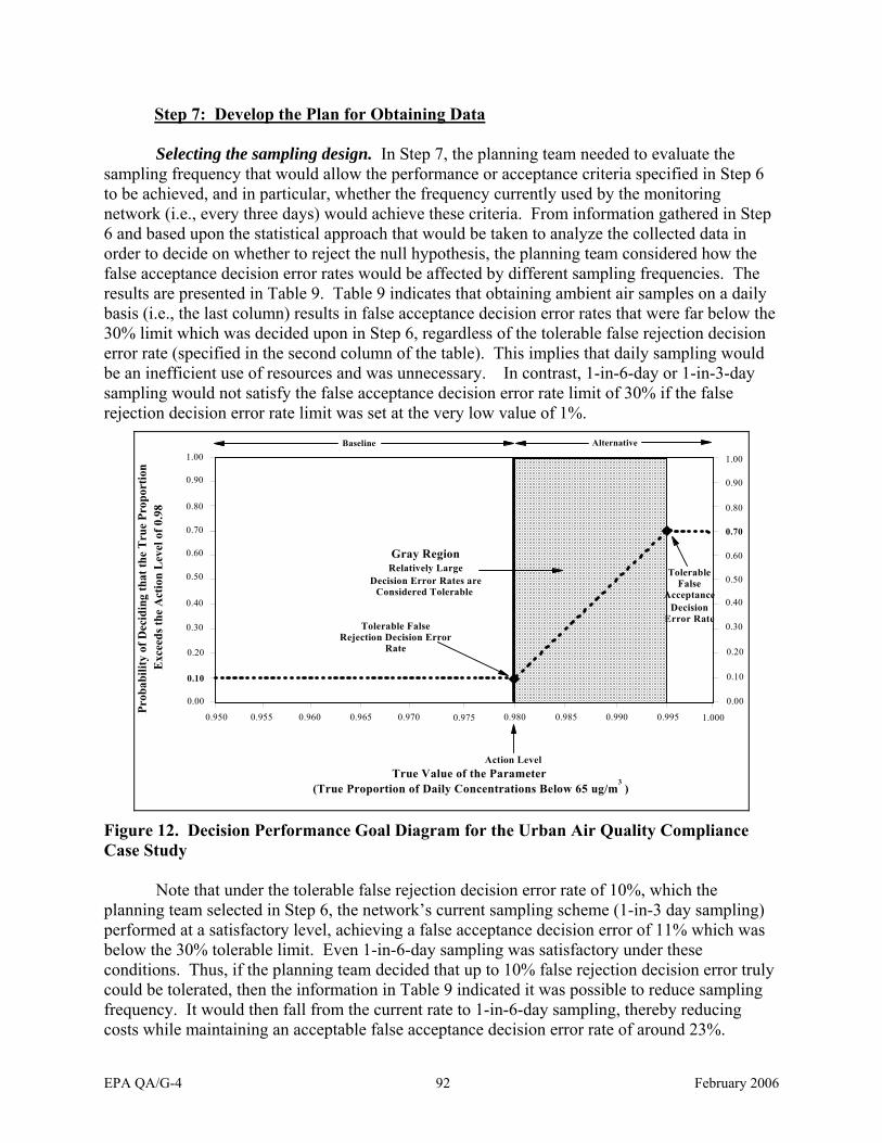
Step 7: Develop the Plan for Obtaining Data

Selecting the sampling design. In Step 7, the planning team needed to evaluate the sampling frequency that would allow the performance or acceptance criteria specified in Step 6 to be achieved, and in particular, whether the frequency currently used by the monitoring network (i.e., every three days) would achieve these criteria. From information gathered in Step 6 and based upon the statistical approach that would be taken to analyze the collected data in order to decide on whether to reject the null hypothesis, the planning team considered how the false acceptance decision error rates would be affected by different sampling frequencies. The results are presented in Table 9. Table 9 indicates that obtaining ambient air samples on a daily basis (i.e., the last column) results in false acceptance decision error rates that were far below the 30% limit which was decided upon in Step 6, regardless of the tolerable false rejection decision error rate (specified in the second column of the table). This implies that daily sampling would be an inefficient use of resources and was unnecessary. In contrast, 1-in-6-day or 1-in-3-day sampling would not satisfy the false acceptance decision error rate limit of 30% if the false rejection decision error rate limit was set at the very low value of 1%.

True Value of the Parameter (True Proportion of Daily Concentrations Below 65 ug/m )

Alternative Baseline


Decision Error Rates are Considered Tolerable

Tolerable False Rejection Decision Error

Rate

Tolerable False

Acceptance Decision

Error Rate

1.00

0.90

0.80

0.70

0.60

0.50

0.40

0.30

0.20

0.10

0.00

0.950 0.955 0.960 0.965 0.970

1.00

0.90

0.80

0.70

0.60

0.50

0.40

0.30

0.20

0.10

0.00

Action Level

0.975 0.980 0.985 0.990 0.995 1.000

Prob

abili

ty o

f Dec

idin

g th

at th

e T

rue

Prop

ortio

nE

xcee

ds th

e A

ctio

n L

evel

of 0

.98

3

Figure 12. Decision Performance Goal Diagram for the Urban Air Quality Compliance Case Study

Note that under the tolerable false rejection decision error rate of 10%, which the planning team selected in Step 6, the network’s current sampling scheme (1-in-3 day sampling) performed at a satisfactory level, achieving a false acceptance decision error of 11% which was below the 30% tolerable limit. Even 1-in-6-day sampling was satisfactory under these conditions. Thus, if the planning team decided that up to 10% false rejection decision error truly could be tolerated, then the information in Table 9 indicated it was possible to reduce sampling frequency. It would then fall from the current rate to 1-in-6-day sampling, thereby reducing costs while maintaining an acceptable false acceptance decision error rate of around 23%.


Specifying key assumptions supporting the selected design. The Information in Table 9 shows the design performance (false acceptance decision error rate) as a function of different possibilities for the tolerable false rejection error rates, and alternative sampling frequencies over a three-year period of data collection. In general, data in Table 9 indicated that the false acceptance decision error rate decreased when a higher false rejection decision error rate was tolerated.

Table 9. False Acceptance Decision Error Rates and Alternative Sampling Frequencies Over a Three-Year Period

Sampling Frequency At Each Of Three Monitors Over a Three-Year Period

1 in 6 Days 1 in 3 Days

(Current Network Frequency)

Every Day

Tolerable False Rejection Decision Error Rates

1% >50% >50% 1%

5% >50% 28% <1%

10% 23% 11% <1%

Similarly, false acceptance decision error rates decreased when sampling intensity was increased from 1-in-6-day sampling to every-day sampling.

9.2 Estimating Mean Drinking Water Consumption Rates for Subpopulations of a City

Background on the Case Study.

The Safe Drinking Water Act Amendments of 1996 require the EPA to identify subpopulations that may have an elevated risk of health effects from exposure to contaminants in drinking water. The assessment of possible elevated risks requires that estimates of mean water consumption per person per day be obtained for subpopulations in the U.S. defined by age, sex, race, socioeconomic status, etc. Typically, a mean drinking water consumption rate of two liters per person per day is used to assess risk. However, this rate represents the general population, and it is less certain if this rate is applicable to certain subpopulations. Currently-available drinking water data are considered inadequate to resolve this issue. Therefore, there is a need to obtain new data to estimate, with specified accuracy and confidence, the mean drinking water consumption rate per person per day for selected subpopulations in the U.S. This information will be used to identify those subpopulations that could have an elevated risk of health effects from exposure to contaminants in drinking water.

To stay within budget constraints, an initial focus will be to collect data for a single city of approximately 1,000,000 inhabitants. This case study consists of a field study that will involve collecting new data to characterize drinking water consumption rates of subpopulations living in this city. It is anticipated that the experience gained from this survey will be useful for developing a survey design that is applicable to a wide range of U.S. cities. As the results will influence multiple drinking water issues, it was decided that the study’s performance criteria


should be specified quantitatively, and that the survey sample size should be determined statistically.


Describing the problem. The problem is to characterize mean drinking water consumption (in liters) per person per day, within specified accuracy and confidence, for subpopulations residing within the city.

Establishing the planning team. The planning team consists of the following:

• A representative of the city’s environmental protection department, who will be responsible for developing the design of the survey, for resolving conflicts and for moving the DQO Process forward,

• A representative of the EPA region in which the city is located, • A social worker who has knowledge of the living and eating patterns of many

subpopulations in the city, • A scientist with experience in developing risk-based surveys of human populations, • A risk assessor who would use the findings of this study as input to mathematical risk

models (data user).

Describing the conceptual model of the potential hazard. Consumption of drinking water can occur either through the direct ingestion of plain (noncarbonated) water (“direct water”), or through adding water to foods and beverages during final preparation at home or by local food service establishments (“indirect water”). In addition to the city’s central water system, selected subpopulations may get their drinking water from various sources, such as private wells or other providers (e.g., water bottlers).

All drinking water contains some impurities. While some of these substances are harmless, others may be classified as contaminants which make water unpalatable or unsafe at certain levels. For example, microbes such as bacteria and viruses can contaminate drinking water. When they are present in water at an elevated level, and the water is consumed at a sufficiently high rate, the resulting ingestion can cause acute health effects, especially in sensitive subpopulations with potentially weakened immune systems. This study will address only drinking water consumption rate and will not extend to estimating health risk from ingesting contaminated water. Estimating risk is a separate problem that will be addressed after the mean drinking water consumption rates have been estimated from the results of this study.

Identifying the general intended use of collected data. The data collected in this study will be used to calculate estimates of mean drinking water consumption per person per day for the selected subpopulations, along with some measure of uncertainty associated with these estimates. Eventually, these estimates would be used as input to models that characterize health risks associated with ingestion and possibly other exposure routes. It follows that the primary use of the study data will be for estimation purposes.


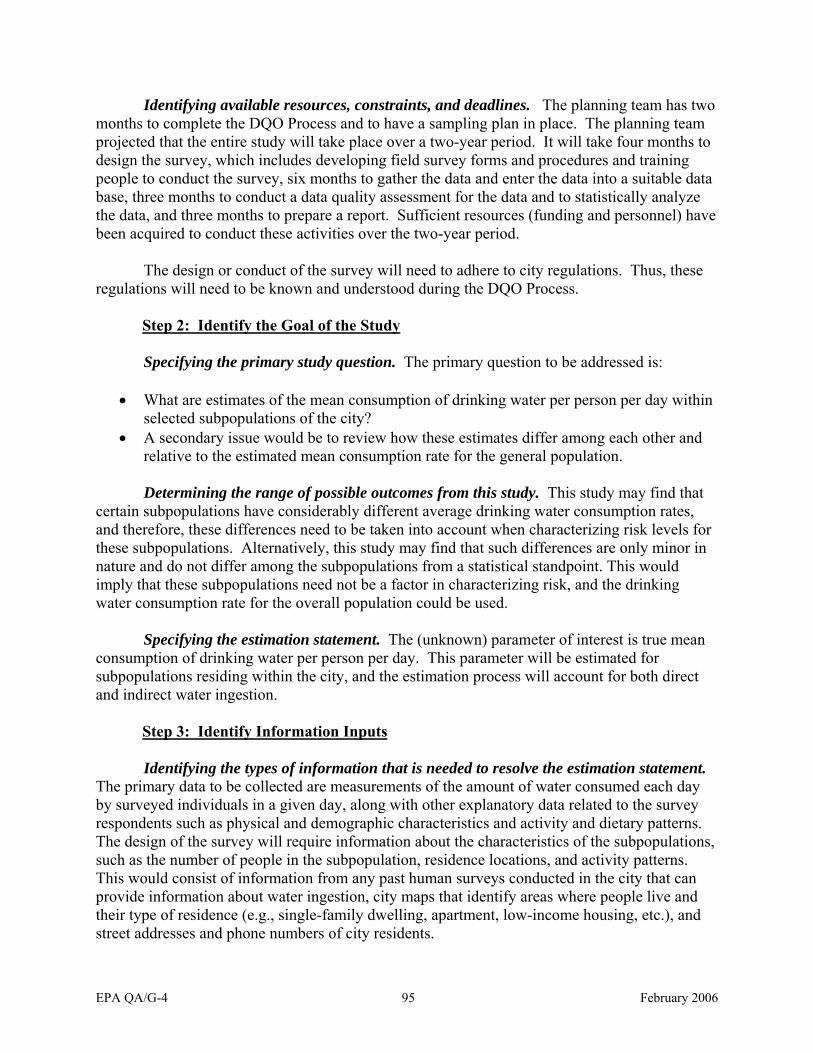
Identifying available resources, constraints, and deadlines. The planning team has two months to complete the DQO Process and to have a sampling plan in place. The planning team projected that the entire study will take place over a two-year period. It will take four months to design the survey, which includes developing field survey forms and procedures and training people to conduct the survey, six months to gather the data and enter the data into a suitable data base, three months to conduct a data quality assessment for the data and to statistically analyze the data, and three months to prepare a report. Sufficient resources (funding and personnel) have been acquired to conduct these activities over the two-year period.

The design or conduct of the survey will need to adhere to city regulations. Thus, these regulations will need to be known and understood during the DQO Process.


Specifying the primary study question. The primary question to be addressed is:

• What are estimates of the mean consumption of drinking water per person per day within selected subpopulations of the city?

• A secondary issue would be to review how these estimates differ among each other and relative to the estimated mean consumption rate for the general population.

Determining the range of possible outcomes from this study. This study may find that certain subpopulations have considerably different average drinking water consumption rates, and therefore, these differences need to be taken into account when characterizing risk levels for these subpopulations. Alternatively, this study may find that such differences are only minor in nature and do not differ among the subpopulations from a statistical standpoint. This would imply that these subpopulations need not be a factor in characterizing risk, and the drinking water consumption rate for the overall population could be used.

Specifying the estimation statement. The (unknown) parameter of interest is true mean consumption of drinking water per person per day. This parameter will be estimated for subpopulations residing within the city, and the estimation process will account for both direct and indirect water ingestion.


Identifying the types of information that is needed to resolve the estimation statement. The primary data to be collected are measurements of the amount of water consumed each day by surveyed individuals in a given day, along with other explanatory data related to the survey respondents such as physical and demographic characteristics and activity and dietary patterns. The design of the survey will require information about the characteristics of the subpopulations, such as the number of people in the subpopulation, residence locations, and activity patterns. This would consist of information from any past human surveys conducted in the city that can provide information about water ingestion, city maps that identify areas where people live and their type of residence (e.g., single-family dwelling, apartment, low-income housing, etc.), and street addresses and phone numbers of city residents.


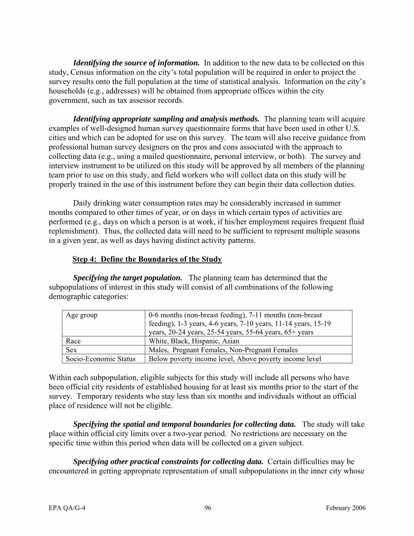
Identifying the source of information. In addition to the new data to be collected on this study, Census information on the city’s total population will be required in order to project the survey results onto the full population at the time of statistical analysis. Information on the city’s households (e.g., addresses) will be obtained from appropriate offices within the city government, such as tax assessor records.

Identifying appropriate sampling and analysis methods. The planning team will acquire examples of well-designed human survey questionnaire forms that have been used in other U.S. cities and which can be adopted for use on this survey. The team will also receive guidance from professional human survey designers on the pros and cons associated with the approach to collecting data (e.g., using a mailed questionnaire, personal interview, or both). The survey and interview instrument to be utilized on this study will be approved by all members of the planning team prior to use on this study, and field workers who will collect data on this study will be properly trained in the use of this instrument before they can begin their data collection duties.

Daily drinking water consumption rates may be considerably increased in summer months compared to other times of year, or on days in which certain types of activities are performed (e.g., days on which a person is at work, if his/her employment requires frequent fluid replenishment). Thus, the collected data will need to be sufficient to represent multiple seasons in a given year, as well as days having distinct activity patterns.


Specifying the target population. The planning team has determined that the subpopulations of interest in this study will consist of all combinations of the following demographic categories:

Age group 0-6 months (non-breast feeding), 7-11 months (non-breast feeding), 1-3 years, 4-6 years, 7-10 years, 11-14 years, 15-19 years, 20-24 years, 25-54 years, 55-64 years, 65+ years

Race White, Black, Hispanic, Asian Sex Males, Pregnant Females, Non-Pregnant Females Socio-Economic Status Below poverty income level, Above poverty income level

Within each subpopulation, eligible subjects for this study will include all persons who have been official city residents of established housing for at least six months prior to the start of the survey. Temporary residents who stay less than six months and individuals without an official place of residence will not be eligible.

Specifying the spatial and temporal boundaries for collecting data. The study will take place within official city limits over a two-year period. No restrictions are necessary on the specific time within this period when data will be collected on a given subject.

Specifying other practical constraints for collecting data. Certain difficulties may be encountered in getting appropriate representation of small subpopulations in the inner city whose


subjects are historically difficult to locate and interview. Constraints such as this will need to be accounted for in the survey design.

Specifying the scale of estimates to be made. Because data will be collected on each individual participating in this study, estimates will be made on an average per person basis for each subpopulation of interest within the city. The collected data will permit estimates to be expressed for a typical 24-hour period.


Developing the specification of the estimator. This study will estimate the true mean drinking water consumption rate per person per day within each specified subpopulation residing within city limits.

The planning team specified that, at a minimum, the following information about each drinking water ingestion data set will be provided for each subpopulation in the survey: the estimated mean, standard error of the estimated mean, 95% confidence limits for the mean, the number of respondents and non-respondents, and graphical displays of the data set (e.g., histograms, box-plots, and probability plots).


The planning team recognizes the key performance criterion as being a specified acceptable level of uncertainty in the estimated mean drinking water consumption rate per person per day within a given subpopulation. Once that desired level of performance is set, an optimal survey design strategy and the required number of subjects for the study can be determined.

The planning team’s risk assessor noted that any risk estimates obtained from mathematical risk models are likely to have large amounts of uncertainty if the level of uncertainty in estimated mean drinking water consumption rates (coming from this study) is too large. Therefore, by working backwards from acceptable levels of uncertainty in risk estimates, the planning team determined that the survey design must allow for the following performance criteria to be achieved:

• The mean drinking water consumption rate will be estimated for each subpopulation to within ±30% of the true mean rate with 95% confidence.

• However, the team recognized that these performance criteria may not be achievable for certain subpopulations because of budget restrictions or because the number of people in some subpopulations may be very small. In these cases, especially if the subpopulation is not deemed to be “critical,” actual performance achieved will simply be documented and will be made available to risk assessors and others who may use the survey results in the future.

Specifying an acceptable level of uncertainty in estimated mean drinking water consumption rates is only one of several important performance and acceptance criteria for this


study. For example, in order to achieve proper representation, the planning team specified that a 90% response rate would be necessary within a given subpopulation.

The survey design process will need to adhere to specific QC procedures to ensure proper design, implementation, and analysis. These QC procedures include checking that (1) the process of selecting people for the survey is implemented properly, (2) the appropriate questions are asked in the appropriate ways, (3) persons conducting the survey are properly recruited and trained, (4) information obtained from persons is accurate and entered correctly into the data base, and (5) software codes used are appropriate for performing required calculations.

Field activities during the survey process (e.g., visiting homes to administer a questionnaire or mailing questionnaires to homes) will need to be audited. This will involve performing follow-up activities such as returning to households where no one was home. The planning team specified that valid data from at least 90% of the people contacted must be obtained.


Selecting the sampling design. The uncertainty in the estimated mean drinking water consumption rates will depend on several factors, including the number of people from which data are obtained and the patterns of variability in consumption rates among people in the subpopulation. An appropriate survey design will help to minimize the effect of variability patterns on the uncertainty of the estimated mean. Also, increasing the number of people in the survey will decrease the uncertainty in the estimated means.

Standard statistics will be utilized to estimate the mean drinking water consumption rates for targeted subpopulations, using statistical survey sampling weights to ensure unbiased results. The planning team specified that a probability-based design will need to be developed and used to select persons to be contacted in the survey.

Based upon the information collected to this point in the DQO Process, the planning team worked together to design the survey. They determined that a minimum of 400 persons in each subpopulation would need to participate in the survey to allow for the mean consumption rate to be estimated to within ±30% of the true mean with 95% confidence. Furthermore, the team did not have sufficient confidence that the required 90% response rate would be achieved if mailed questionnaires were used to obtain the data. Thus, they decided that persons in the survey would be interviewed in their homes by trained field data collectors, with appropriate follow-up activities taking place if no response was obtained (e.g., returning to households at a later time if no one was home at the time of the visit). They noted that certain subpopulations are scattered in different sections of the city, while others were grouped together in certain districts.

Taking this information and considerations of cost and budget into account, the team determined that a multi-stage, cluster sampling design would most likely achieve the performance criteria. This design involves first selecting a set of city blocks using simple random sampling, then selecting a set of homes within each selected block using simple random sampling, and finally, interviewing each person in the home that is a member of a subpopulation


of interest. For subpopulations that live mostly within certain districts, the design would be applied to only those districts. The formulae that must be used to estimate the mean drinking water consumption rate for a multi-stage, cluster design will be developed using information from references on statistical sampling designs.

All of this design information, along with the methods that will be used to conduct the survey, will be determined and documented within a QA Project Plan. This QA Project Plan will then be properly implemented by the study team, with all QA-related procedures properly monitored by the study’s QA manager, in order to provide an appropriate level of confidence that the survey results are credible, unbiased, and meaningful. The results of the survey will be documented in a report that includes information on non-response rate and any caveats that are observed in interpreting the data.

Specifying key assumptions supporting the selected design. The targeted sample size for each subpopulation in this study was calculated based on published methods. In this case, the planning team indicated a prespecified relative standard deviation of η = 3 (where η = σ/ μ is the coefficient of variation, μ is the true mean consumption rate, and σ = 6 is the standard deviation of the mean consumption rate). Then, the relative error is specified as dr = | X - μ |/ μ such that Prob[ | X - μ | ≥ dr μ ] = α. For this study, dr = 0.30 and α=0.05 (i.e., within ±30% of the true mean with 95% confidence). The corresponding formula for calculating the sample size for each subpopulation is given as

n = (z1−α / 2 .η / dr )

2

+ 21 (z1−α / 2 .η / dr ) / N

where z0.975 = 1.96 and N = 1,000,000. Computing this formula gives n = 384 (~400) as an approximate sample size for each subpopulation.

The approach to calculating uncertainty in each estimated mean involves using the drinking water ingestion data to calculate the standard error of the mean consumption rate and using it, along with information about the shape of the underlying distribution of the consumption rate data, to compute a 95% confidence interval for the true mean. If the data are found to be normally distributed and no sampling problems are encountered, then standard techniques will be used to compute this confidence interval. If there are anomalies in sampling or the data are not normally distributed, then special formulas will need to be identified and/or constructed.

The consumption rate data sets for the various subpopulations will be graphically summarized and compared using histograms, box plots, and probability plots. These graphs can be used to visually assess whether the data are normally distributed and whether there may be differences in mean consumption rates among subpopulations. Although the primary purpose of the survey is not to detect differences in consumption rate means among subpopulations, the graphical and other data analyses may suggest hypotheses about possible differences that may need to be evaluated more thoroughly using a special survey at a later time.


9.3 Household Dust Lead Hazard in Athington Park House, Virginia

Background on the Case Study.

Athington Park House is a very desirable property that was built some years before the discontinuing of lead in paint in the mid-1970s. The current owners are concerned about the possible presence of lead in dust contained in the house.

The adverse health effects resulting from exposure to lead hazards (paint, dust, and soil) have received increasing attention because chronic exposure to low levels of lead can cause impairment of the central nervous system, mental retardation, and behavioral disorders. Young children (below the age of six) are at a particularly high risk for these adverse effects. Concern about the exposure to lead hazards in residential housing has led federal agencies, including the EPA and Department of Housing and Urban Development, to develop programs to evaluate, and ultimately control, lead hazards in housing.

A critical pathway for exposure to lead by a child is through the ingestion of household dust because dust collects on hands, toys, and food and is easily transferred by hand-to-mouth activities. As a result of the concern about the dust-to-mouth pathway, an important component of risk assessment is dust sampling. Dust sampling offers a way of characterizing dust lead levels at a property and determining if intervention is warranted. One of the preferred methods for sampling residential dust is using baby wipes to wipe a specified surface area. A single area may be sampled using an individual wipe; or multiple areas of a room may be sampled with individual wipes, and the individual wipes combined, or composited, then submitted to the laboratory as a single sample (40 CFR 745). The distribution of dust lead levels is such that normality cannot be assumed and a 50th percentile (the median) is the appropriate risk assessment level.


Describing the problem. The owners wish to evaluate the potential hazards associated with lead in dust in a single-family residence because other residences in the Athington Park House neighborhood had shown levels of lead in dust that might pose potential hazards.

Establishing the planning team. The planning team included the property owners, a certified risk assessor (to collect and handle dust samples and serve as a liaison with the laboratory), and a quality assurance specialist. The decision makers were the property owners.

Describing the conceptual model of the potential hazard. The conceptual model described a single-family residence in a neighborhood where hazardous levels of lead had been detected in other residences. Interior sources of lead in dust were identified as lead-based paint on doors, walls, and trim, which deteriorated to form, or attach to, dust particles. Exterior sources included lead in exterior painted surfaces that had deteriorated and leached into the dripline soil, or lead deposited from gasoline combustion fumes that accumulated in soil. In these cases, soil could be tracked into the house, and collected as dust on floors, window sills,


toys, etc. As this dust could be easily ingested through hand-to-mouth activities, dust was considered to be a significant exposure route. Levels of lead in floor dust were to be used as an indicator of the potential hazard.

Identifying the general intended use of collected data. The data collected in this study will be used to determine if a heath hazard is present at Athington Park House using the criteria established under 40 CFR 745. This is a decision making (test of hypothesis) DQO Process.

Identifying available resources, constraints, and deadlines. The property owners were willing to commit up to $1,000 for the study. To minimize inconvenience to the family, all sampling would be conducted during one calendar day.


Specifying the primary study question. The primary question to be addressed is to determine if there were significant levels of lead in floor dust at the House.

Determining the range of possible outcomes from this study. If there were significant levels of lead in floor dust at the residence, the team planned follow-up testing to determine whether immediately dangerous contamination exists and the location of the contamination in the property. If not, then there was no potential lead hazard, and testing would be discontinued.


Identifying the types of information that is needed to resolve the decision statement. The assessment of a dust lead hazard would be evaluated by measuring dust lead loadings by individual dust wipe sampling according to established protocol.

Identifying the source of information. The EPA proposed standard stated that if dust lead levels were above 50 μ / t 2g f on bare floors, a lead health hazard was possible and follow-up testing and/or intervention should be undertaken (40 CFR 745).

Identifying how the Action Level will be determined. The Action Level is the EPA standard specified in 40 CFR 745.

Identifying appropriate sampling and analysis methods. Wipe samples were collected according to ASTM standard practice E1728. These samples were digested in accordance with ASTM standard practice E1644 and the sample extracts were chemically analyzed by ASTM standard test method E1613. The results of these analyses provided information on lead loading (i.e., μg of lead per square foot of wipe area) for each dust sample. The detection limit was well below the Action Level.


Specifying the target population. The planning team has determined that the subpopulations of interest in this study will consist of all combinations of the following demographic categories:


Age group 0-6 months (non-breast feeding), 7-11 months (non-breast feeding), 1-3 years, 4-6 years, 7-10 years, 11-14 years, 15-19 years, 20-24 years, 25-54 years, 55-64 years, 65+ years

Race White, Black, Hispanic, Asian Sex Males, Pregnant Females, Non-Pregnant Females Socio-Economic Status Below poverty income level, Above poverty income level

Within each subpopulation, eligible subjects for this study will include all persons who have been official city residents of established housing for at least six months prior to the start of the survey. Temporary residents who stay less than six months and individuals without an official place of residence will not be eligible.

Specifying the spatial and temporal boundaries for collecting data. The spatial boundaries of the study area were defined as all floor areas within the dwelling that were reasonably accessible to young children who lived at, or visited, the property. Dust contained in each one ft.2 area of each floor of the residence was sampled and sent to a laboratory for analysis.

Specifying other practical constraints for collecting data. Permission from the residents of Athington Park House was required before risk assessors could enter the residence to collect dust wipe samples. Sampling was completed within 1 calendar day to minimize the inconvenience to the residents.

Specifying the scale of estimates to be made. The test results were considered to appropriately characterize the current and future hazards. It was possible that lead contained in soil could be tracked into the residence and collect on surfaces, but no significant airborne sources of lead deposition were known in the region. The dust was not expected to be transported away from the property; therefore, provided the exterior paint was maintained in intact condition, lead concentrations measured in the dust were not expected to change significantly over time.

Specifying the scale of inference for decision making. The decision unit was the interior floor surface (approximately 1,700 ft2) of the residence at the time of sampling and in the near future.


Specifying the Action Level. This was given in 40 CFR 745 which specified 50 μ / t 2g f .

Developing the population of interest and the theoretical decision rule. From 40 CFR 745, the median was selected as the appropriate parameter to characterize the population under study. The median dust lead loading was defined to be that level, measured in μg/ft2, above and below which 50% of all possible dust lead loadings at the property were expected to fall. If the true median dust loading in the residence was greater than 50 μ / t 2g f , then the planning team required followup testing. Otherwise, they decided that a dust lead hazard was not present and discontinued testing.



Setting the baseline condition. The baseline condition adopted by the property owners was that the true median dust lead loading was above the EPA hazard level of 50 μ / t 2g f , due to the seriousness of the potential hazard. The planning team decided that the most serious decision error would be to decide that the true median dust lead loading was below the EPA hazard level of 50 μ / t 2g f , when in truth the median dust lead loading was above the hazard level. This incorrect decision would result in significant exposure to dust lead and adverse health effects.

Determining the impact of decision errors and setting tolerable decision error limits. The edge of the gray region was designated by considering that a false acceptance decision error would result in the unnecessary expenditure of scarce resources for follow-up testing and/or intervention associated with a presumed hazard that did not exist. The planning team decided that this decision error should be adequately controlled for true dust lead loadings of 40 μ / t 2g f and below. Since human exposure to lead dust hazards causes serious health effects, the planning team decided to limit the false rejection error rate to 5%. This meant that if this dwelling=s true median dust lead loading was greater than 50 μ / t 2g f , the baseline condition would be correctly rejected 19 out of 20 times. The false acceptance decision, which would result in unnecessary use of testing and intervention resources, was allowed to occur more frequently (i.e., 20% of the time when the true dust-lead loading is 40 μ / t 2g f or less). These are shown in Figure 13.


Selecting the sampling design. The planning team determined that the cost of sending a certified risk assessor to the property for collecting and handling dust wipe samples was about $400. Also, an NLLAP-recognized laboratory was selected to analyze the collected wipe samples at a cost of $10 per sample. Thus, a maximum of 60 samples could be obtained within the study=s cost constraint of $1,000. From Step 6 the initial gray region lower bound for the study was set at 40 μ / t 2g f , but, the team found that this requirement could not be met given the specified decision errors (i.e., false rejection rate of 5% and false acceptance rate of 20%), assumed standard deviation (of the natural logarithms), range, and cost constraints of the study (i.e., a maximum of 60 samples). The planning team decided they were unwilling to relax the decision error rate requirements and elected to expand the width of the gray region from the original 40 to 50 μ / t 2 to the less restrictive range of 35 to 50 μg ft 2 . Further, the planningg f /team decided that a standard deviation (of the natural logarithms) value of σ=1.0 was probably more realistic than the more conservative estimate of σ=1.5.

The planning team used the upper variability bound to develop Table 10 which presented statistical sample size requirements across various assumed dust lead loading standard deviations (of the natural logarithms) and various lower bounds of the gray region. This table indicated that sample size requirements increased rather dramatically as variability increased and/or as the gray region was made more narrow.


Therefore, based on Table 10, the planning team decided that a total of 50 samples should be collected by a certified risk assessor (all within 1 calendar day) using simple random sampling throughout the residence. Samples were sent to the selected NLLAP-recognized laboratory for analysis. The total study cost was approximately $900 to the property owners.

Alternative Baseline


Decision Error Rates are Considered Tolerable Tolerable False

Acceptance Decision Error Rate

Tolerable False Rejection Decision Error Rates

1.00

0.90

0.80

0.70

0.60

0.50

0.40

0.30

0.20

0.10

0.00

1.00

0.90

0.80

0.70

0.60

0.50

0.40

0.30

0.20

0.10

0.00

0.95

Prob

abili

ty o

f Dec

idin

g th

at th

e T

rue

Med

ian

Exc

eeds

th

e A

ctio

n L

evel

of 5

0 ug

/ ft 2

0 10 20 30 40 50 60 70 80 90 100

Action Level

True Value of the Parameter (Median Dust-lead loading, ug/ft2 )

Figure 13. Decision Performance Goal Diagram for Lead Dust Loading

Table 10. Number of Samples Required for Determining If the True Median Dust Lead Loading is Above the Standard

Gray Region (μg/ft2)

Standard Deviation of Natural Logarithms σ=0.5 σ=1.0 σ=1.5

20-50 6 9 13

25-50 8 15 21

30-50 14 26 37

35-50 26 50 75

40-50 64 126 188

45-50 280 559 837


Specifying key assumptions supporting the selected design. The dust lead loading data was assumed to be log-normally distributed. The geometric mean was computed using the data because the true median and true geometric mean are the same when log-normality is assumed. The true variability in dust lead loadings was not known, but past data was used to estimate a reasonable upper bound on variability.


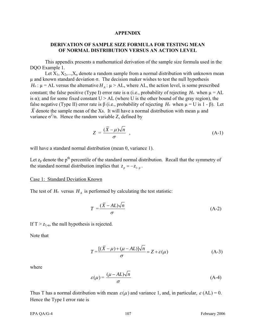
APPENDIX

DERIVATION OF SAMPLE SIZE FORMULA FOR TESTING MEANOF NORMAL DISTRIBUTION VERSUS AN ACTION LEVEL

This appendix presents a mathematical derivation of the sample size formula used in the DQO Example 1. Let X1, X2,...,Xn denote a random sample from a normal distribution with unknown mean µ and known standard deviation σ. The decision maker wishes to test the null hypothesis Ho : µ = AL versus the alternative H A : µ > AL, where AL, the action level, is some prescribed constant; the false positive (Type I) error rate is α (i.e., probability of rejecting Ho when µ = AL is α); and for some fixed constant U > AL (where U is the other bound of the gray region), the false negative (Type II) error rate is β (i.e., probability of rejecting Ho when µ = U is 1 - β). Let X denote the sample mean of the Xs. It will have a normal distribution with mean µ and variance σ2/n. Hence the random variable Z, defined by

(X − μ) n Z = , (A-1)σ

will have a standard normal distribution (mean 0, variance 1).

Let zp denote the pth percentile of the standard normal distribution. Recall that the symmetry of the standard normal distribution implies that zp = −z1− p .

Case 1: Standard Deviation Known

The test of Ho versus H A is performed by calculating the test statistic:

(X − AL) n T = (A-2) σ

If T > z1-α, the null hypothesis is rejected.

Note that

[(X − +μ μ) ( − A L )] nT = = +Z ε ( )μ (A-3) σ

where (μ − AL) n ε ( )μ = (A-4)

σ

Thus T has a normal distribution with mean ε ( ) μ and variance 1, and, in particular, ε (AL) = 0.Hence the Type I error rate is


Pr[rejecting H H o | o] = Pr[ T > z 1−α | μ = AL] P= r[ Z + ε (AL) > z 1−α ] P= r[ Z > z 1−α ] (A-5)

Achieving the desired power 1- β when µ = U requires that

Pr[reject Ho | µ = U] = 1 – β.

Therefore,

Pr[ T z ≤ 1−α | μ = U ] P= r[ Z + ε (U ) ≤ z 1−α ] P= r[ Z ≤ z 1−α − ε ( U )] = β (A-6)

This implies

z1−α - ε ( )μ = zβ ,

or

( U A− L) n z1−α − = −z β σ 1−

Let d = U-AL, then rearrange terms to obtain

(z1−α + z1−β )σ = d n or

(z1−α + zn = 1−β )

2σ 2

(A-7)d 2

Case 2: Standard Deviation Unknown

If the standard deviation σ is unknown, then a test statistic such as Equation A-2 is used except that σ is replaced by s, an estimate of the standard deviation calculated from the observed Xs. Such a statistic has a noncentral t distribution rather than a normal distribution, and the n computed by the above formula will be too small, although for large n (say n>40), the approximation is good. The particular noncentral t distribution involved in the calculation depends on the sample size n. Thus, determining the exact minimum n that will satisfy the Type I and Type II error rate conditions requires an iterative approach in which the noncentral t probabilities are calculated for various n values until the desired properties are achieved. With the aid of a computer routine for calculating such probabilities, this is not difficult; however, a simple and direct approach for approximating n is available. This approach, whose derivation is described in the paragraphs below, leads to the following approximate but very accurate formula for n:


(z1−α + z1−β )2σ 2 1n = 22 + z (A-8)

d 2 1−α

In practice, since σ is unknown, a prior estimate of it must be used in Equation A-8.

The approach is based on the assumption that, for a given constant k, the statistic is approximately normal with mean µ-kσ and variance ( 2σ /n)(1+k2/2) (Guenther, 1977 and 1981).

The classical t-test rejects H0 when, T = [(X − AL ) / s n] > D where the critical value D is chosen to achieve the desired Type I error rate α. The inequality can be rearranged as X − ks > AL , where k D= n . Subtracting the mean (assuming H0) and dividing by the standard deviation of X − ks on both sides of the inequality leads to

X − −ks (A L − kσ ) AL − (AL − kσ ) k n> = (A-9)

( / σ n) 1 + k 2 / 2 ( /σ n) 1 + k 2 / 2 1+ k 2 / 2

By the distributional assumption on X − ks , the left side of Equation A-9 is approximately standard normal when µ = AL, and the condition that the Type I error rate is α becomes

Pr[ Z k> n / 1 + k 2 / 2] = α (A-10)

i.e., z1−α = k n / 1+ k 2 / 2 (A-11)One can show that Equation A-11 is equivalent to

1 [− +1 k 2 / 2] = (1 − z2 1−α ) / 2 n (A-12)

The condition that the Type II error rate is β (or that power is 1-β) when µ = U means that the event of incorrectly accepting H0 given X − ks should have probability β. Subtracting the mean (U - kσ) and dividing by the standard deviation of X − ks on both sides of this inequality yields

X − −ks (U − kσ ) AL − (U − k σ ) ≤ (A-13)

( /σ n ) 1 + k 2 / 2 ( / σ n) 1 + k 2 / 2

Again, the left side is approximately standard normal and the Type II error rate condition becomes

Pr{ Z ≤ [AL − (U − kσ )] /[( σ / n ) 1 + k 2 / 2]} = β


which implies

(AL −U ) + kσ ) −z1−β = zβ = (A-14)

( / σ n) 1 + k 2 / 2

Subtracting Equation A-14 from Equation A-11 yields

( U A− L ) z1−α + z1−β = (A-15)( / σ n ) 1 + k 2 / 2

or

(z1−α + z1−β )σ n = (A-16)

( U A− L ) 1+ k 2 / 2

Substituting Equation A-12 into the denominator on the right side of Equation A-16 yields

(z1−α + z1−β )σ = n 1− z2 / 2 n (A-17)

( U A− L ) 1−α

Squaring both sides of Equation A-17 and solving for n yields Equation A-8.

References

Guenther, William C. 1977. Sampling Inspection in Statistical Quality Control. Griffin's Statistical Monographs and Courses, No. 37, London: Charles Griffin.

Guenther, William C. 1981. Sample size formulas for normal theory T test. The American Statistician, Vol. 35, 4.


REFERENCES

U.S. Environmental Protection Agency, 1996. Soil Screening Guidance: User’s Guide.

U.S. Environmental Protection Agency, 2000a. Guidance for the Data Quality Objectives Process (EPA QA/G4).

U.S. Environmental Protection Agency, 2000b. Policy and Program Requirements for the Mandatory Agency-Wide Quality System, EPA Order 5360.1 A2.

U.S. Environmental Protection Agency, 2000c. EPA Quality Manual for Environmental Programs, EPA Manual 5360 A1.

U.S. Environmental Protection Agency, 2000d. Guidance on Technical Audits and Related Assessments for Environmental Data Operations (EPA QA/G-7). EPA/600/R-99/080.

U.S. Environmental Protection Agency, 2001a. Decision Error Feasibility Trials (DEFT) Software (EPA QA/G-4D). EPA/240/B-01/007.

U.S. Environmental Protection Agency, 2001b EPA Requirements for Quality Assurance Project Plans (EPA QA/R-5). EPA/240/B-01/003.

U.S. Environmental Protection Agency, 2001c. Guidance on Preparing Standard Operating Procedures (EPA QA/G-6). EPA/240/B-01/004.

U.S. Environmental Protection Agency, 2002a. Guidelines for Ensuring and Maximizing the Quality, Objectivity, Utility, and Integrity of Information Disseminated by the Environmental Protection Agency.

U.S. Environmental Protection Agency, 2002b. Overview of the EPA Quality System for Environmental Data and Technology.

U.S. Environmental Protection Agency, 2002c. Guidance for Choosing a Sampling Design for Environmental Data Collection (EPA QA/G-5S). EPA/240/R-02/005.

U.S. Environmental Protection Agency, 2002d. Guidance on Quality Assurance Project Plans (EPA QA/G-5). EPA/240/R-02/009,

U.S. Environmental Protection Agency, 2003. Summary of General Assessment Factors for Evaluating the Quality of Scientific and Technical Information.

U.S. Environmental Protection Agency, 2006a. Data Quality Assessment: A Reviewer’s Guide (EPA QA/G-9R).

U.S. Environmental Protection Agency, 2006b. Data Quality Assessment: Statistical Tools for Practitioners (EPA QA/G-9S).
