GROUND-PENETRATING RADAR INVESTIGATION

OF PREFERENTIAL FLOWPATHS ON A HILLSLOPE

by

STEPHAN DAVID FITZPATRICK

(Under the direction of John F. Dowd)

ABSTRACT

A hillslope investigation took place for the purpose of confirming correlation between

ground-penetrating radar returns and stormflow. A sprinkler system was operated over a 280 by

200 cm area of the slope in order to generate subsurface flow. Through previous investigations a

kinematic response had been shown to rapidly mobilize high rates of runoff. It had been found that

a threshold condition occurred near saturation which activated the kinematic pressure wave. For

our experiment this process drove delivery through preferential flowpaths into a runoff gutter

collection system. Temperature changes and rainfall rates were monitored as well as volumetric

rates of response. Radar returns were processed and examined afterward. A separate soil core

experiment was also conducted under laboratory conditions. This was done to characterize the

retentivity of the soil since antecedent soil moisture makes up the majority of the water that

becomes mobilized. Comparisons between hydrological and radar data were made utilizing the

gathered information.

INDEX WORDS: soil-moisture, groundwater, ground-penetrating radar, kinematic

GROUND-PENETRATING RADAR INVESTIGATION

OF PREFERENTIAL FLOWPATHS ON A HILLSLOPE

by

STEPHAN DAVID FITZPATRICK

A.B., University of Georgia, 2008

A Thesis Submitted to the Graduate Faculty of The University of Georgia in Partial

Fulfillment of the Requirements for the Degree

MASTER OF SCIENCE

ATHENS, GEORGIA

2011

© 2011

Stephan David Fitzpatrick

All Rights Reserved

GROUND-PENETRATING RADAR INVESTIGATION

OF PREFERENTIAL FLOWPATHS ON A HILLSLOPE

by

STEPHAN DAVID FITZPATRICK

Major Professor: John F. Dowd Committee: Ervan G. Garrison Todd C. Rasmussen

Electronic Version Approved:

Maureen Grasso Dean of the Graduate School The University of Georgia May 2011

iv

ACKNOWLEDGEMENTS

Initial gratitude must be given to my major professor, Dr. John Dowd. This research, my

progress through graduate school, is due in large part to his looming intellectual presence,

abundant humor and generous support.

I want to give forth my sincerest thanks to the other two members of my committee for

their invaluable support and insight: Dr. Ervan Garrison and Dr. Todd Rasmussen. I would also

like to thank Dr. Larry Morris who provided me with a Tempe cell array and laboratory when

they were necessary and Leigh Ogden for help with said resources. I value the knowledge and

support I gained from UGA faculty members Bill Miller, David Radcliffe and Paul Schroeder.

My appreciation goes out to the Joseph Berg, Bernadette and Gilles Allard, and Miriam

Watts-Wheeler committees. These awards were valuable to my research.

Additional gratitude has to go out to the staff at the USDA-ARS J. Phil Campbell Sr.

Natural Resources Conservation Center, especially Steve Norris who was always there for us.

Additional thanks goes to Dinku Endale for hosting me and my efforts. I also thank Dory

Franklin, Dwight Seman and Mike Thornton at USDA-ARS.

I want to thank Jessica Cook for her invaluable help in getting the all things GPR-related

done. I would also like thank Liz Cary Purvis and subsequently Bonnie Purvis Nobles of Metal

F-X Manufacturing for their support.

Then there is my research partner, Ernest “Bubba” Beasley: thank you my friend!

It got done through the love, patience and support of my immediate family (Anne-Marie

Fitzpatrick, Lt. Col. Adrian Fitzpatrick, and Marina Fitzpatrick), my family-at-large, and my

friends: you know who you are.

v

TABLE OF CONTENTS

Page

ACKOWLEDGEMENTS...............................................................................................................iv

LIST OF FIGURES.......................................................................................................................vii

CHAPTER

1 INTRODUCTION...................................................................................................1

2 LITERATURE REVIEW.........................................................................................7

Overview………………………………………………………………......7

Kinematic pressure wave generation……………...……………………..10

Soil moisture retentivity………………………….……………..………..12

Contributions to runoff……………………..……..……………………..15

Preferential flow due to macropores…………………….…......………...17

Ground-penetrating radar utilization……………………………..………20

3 SITE DESCRIPTION............................................................................................24

Overview…………………………………………………………………24

Climate…………………………………………………………………...26

Soil……………………………………………………………………….27

4 METHODS............................................................................................................28

Overview………….………………………………………………...……28

Gutter and data collection system…………………………………......…28

Plot-scale ground-penetrating radar……………………………………...32

Ground-penetrating radar survey timeline……………………..…...……34

vi

Tempe cell experiment…………………………………………..……….38

5 DATA AND RESULTS..........................................................................................40

Ground-penetrating radar returns………………………………………...40

Micrologger data………………………………………………………....43

Soil-moisture retentivity curve……………………...………………..….45

Miscellaneous data……………………………...……………..…………47

6 DISCUSSION OF RESULTS……………………………………….…………...49

Overview……………………………………………………..…………..49

Resolution of radar signal………………………………………………..50

Images from radar returns………………………………………………..52

Data analysis from radar returns…………………………..……………..55

7 CONCLUSIONS AND FUTURE WORK………….….......................................64

REFERENCES..............................................................................................................................67

APPENDICES

A GROUND-PENETRATING RADAR AND TRACER EXPERIMENT

TIMELINE.............................................................................................................75

B RADAR RETURNS…………………………………………………………….78

C TEMPE CELL DATA…………………………………………………...……...138

D MODELED RESOLUTION IN CM VERSUS SOIL DIELECTRIC CONSTANT

DURING VARIABLE WETTING PERIODS.....................................................139

vii

LIST OF FIGURES

Page

Figure 1: Table of dielectric constants and propagation velocities for certain materials…….........4

Figure 2: Buckinghams’ original soil-moisture release curve…………………………………….7

Figure 3: "Ground-penetrating radar soil suitability map of the conterminous United States”…...9

Figure 4: The kinematic wave process in a small soil core………………………………….…...11

Figure 5: Van Genuchten’s retentivity curve…………………………………………………….14

Figure 6: Schematic diagram of Hewlett and Hibbert's soil model………………...……………16

Figure 7: Diagram of flow within macropore space…………………………………………..…19

Figure 8: GPR-derived map of an impervious clay layer and inferred flow pathways………….23

Figure 9: The Northeast Georgia Inner Piedmont……………………………………………..…24

Figure 10: The convergent zone in Experimental Pasture 1E………………………………..…..25

Figure 11: Gridded plot for GPR survey…………………………………………………..……..26

Figure 12: The Ap horizon in the convergent zone………………..……………………………..27

Figure 13: Gutter collection setup………………………………………………………..………28

Figure 14: Gutter design…………………………………………………………………………29

Figure 15: ONSET tipping bucket in collection pit..…………………………………………….30

Figure 16: Location of thermistors relative to the gutter ……………………..…………..……..31

Figure 17: Campbell CR23X Micrologger………………………………………………………32

Figure 18: Schematic of GPR antennae and various wave travel paths…………………………34

Figure 19: Tlaloc 3000 sprinkler system over gridded plot……………………………………...36

vii

Figure 20: Antenna operation for GPR survey………………………………………..…………37

Figure 21: Typical Tempe cell array…………………………………………………..………....38

Figure 22a: Radar return examples from GPR survey A, 6/7/2010, 1338 EDT……….,…..……41

Figure 22b: Radar return examples from GPR survey I, 6/10/2010, 1409 EDT………………...42

Figure 22c: Radar return examples from GPR survey L, 6/13/2010, 1557 EDT………………..42

Figure 23: Thermistor, discharge, rain, sprinkler activation and run information………………45

Figure 24a: Soil-moisture retentivity curve, 0-6 cm depth……………………………..……..…47

Figure 24b: Soil-moisture retentivity curve, 5-11 cm depth……………………..…………...….47

Figure 25: Modeled radar resolution as a function of dielectric constant during wetting……….52

Figure 26: Returns before (K), immediately after (L) and hours after first response (M)……….53

Figure 27a: Dispersion of signal due to depth: Run A (left near top; right near bottom)………...54

Figure 27b: Dispersion of signal due to depth: Run L (left near top; right near bottom)………..55

Figure 28a: Intensity and frequency by layer, Layer 9, Runs A-D (5-6 cm)………..…………...57

Figure 28b: Intensity and frequency by layer, Layer 9, Runs J-M (5-6 cm)…………..………...58

Figure 28c: Intensity and frequency by layer, Layer 19, Runs A-D (11-12 cm)…….……...…...58

Figure 28d: Intensity and frequency by layer, Layer 19, Runs J-M (11-12 cm)………...…..…...59

Figure 29a: Intensity and frequency by depth, Run A…………………………………………...60

Figure 29b: Intensity and frequency by depth, Run K…………………………………………...61

Figure 29c: Intensity and frequency by depth, Run L…………………………………………...61

Figure 29d: Intensity and frequency by depth, Run M………………………………...………...62

1

CHAPTER 1

INTRODUCTION

During upland storm events groundwater has the capacity to become rapidly mobilized in

the form of subsurface runoff. Research, which began in the 1960's, confirms that both lateral

runoff and antecedent soil-moisture make significant contributions to hillslope hydrological

processes. The overall volumes as well as timing of runoff are similar to that observed in

overland runoff. This stormflow occurs as interflow (a “catch-all” term) which occupies the

region between baseflow and overland flow on a storm hydrograph. This subsurface runoff

makes significant contributions to streamflow: the ultimate destination for most watershed

runoff. Isotopic studies have shown that “old water”, pre-existent to the given storm event,

constitutes much of this runoff. Antecedent soil moisture is translated, or forced, down the

hillslope through the precipitation striking entering the system. Research suggests that a local

kinematic response to rainfall acts as the initial mechanism for this runoff (Williams, et al, 2002).

Once the kinematic response is initiated water may move laterally along preferential flowpaths.

These flowpaths may take the form of macropore networks or some other structural

feature that encourages interflow. Unstable wetting fronts lead to “fingered flow” development

in the upper soil profiles (Selker, et al, 1992). This often occurs because the matric potential

(analogous to “negative pressure” or “suction”) gradient opposes the direction of flow.

Preferential flow and unstable wetting fronts are also attendant to heterogeneities in the soil.

Fingered flow often forms during infiltration pathways but these also occur as sub-horizontal

flows as well.

2

The development of macropores in the soil exacerbates rapid delivery. Macropores are

minute structures: areas of increased porosity and permeability. They generally take the form of

tunnel, pore, or fracture structures ranging in diameter from 3 x 10-6 to 3 x 10-4 cm. These

structures may allow for increased preferential flow when pathways are interconnected.

Regardless, it must be kept in mind that the development of these structures can be problematic.

They are easily destroyed by the activity of flora and fauna as well as human activity. Soil

development itself can inhibit macropore development. Clay content in soils, by its very nature,

may act to form impermeable barriers within these channels. The constant drying and wetting

associated with certain soils can also alter macropore structure.

Investigation of the kinematic pressure wave phenomenon as a mechanism for runoff

generation has come about fairly recently. Precipitation is the initial impetus for rapidly

mobilized water, usually through storms of heightened intensity. Pressure waves are propagated

in unsaturated media due to perturbations in the volumetric pore-water content of the soil. The

kinematic velocity or celerity, the wave velocity, is the derivative of the darcian flux with respect to

the water content. It can be used to predict the pressure-driven velocity of fluid pulses in a system.

Small inputs can trigger rapid hydraulic responses due to this phenomenon (Rasmussen, et al.,

2000). Translation of pressure, or energy, waves were found to lead to these responses within

homogeneous media in the unsaturated zone. This response literally pushes old water, or

antecedent soil-moisture, laterally down the hillslope. Water held in tension at negative pressure

attains positive downward pressure.

The two preferential flow mechanisms- interflow and translatory flow- are well

documented. Through the use of hydrological models and hydrological field methods the influence

these mechanisms can be accurately inferred but rarely directly. The direct visualization of

3

subsurface flowpaths in situ would be highly favorable as would subsurface data relating to flow.

Nevertheless in order to make direct observations the soil itself would have to be disturbed which

would likely destroy structures allowing for interflow, especially macropores. Doing so would also

alter the continuity of the system itself. The minute structures that allow for preferentially flow are

exceedingly fragile having developed over many years due to soil formation factors: parent

material, topography, climate, biological influence and slope aspect. Although bulk chemical and

physical characteristics of a soil can be analyzed in a laboratory setting by taking core samples,

actual flowpath structure cannot easily be observed or even inferred in such a manner. Furthermore

preferential flow pathways are often transient and dependent on specific conditions that occur

during a variety of time-dependent events. Different sorts of methods must be used to observe

preferential flowpaths. Geophysical investigation is one such set of methodologies.

There are a variety of geophysical methods available for detecting groundwater and soil-

moisture. Since World War II various types of instrumentation have been used to assess soil-water.

Electromagnetic sounding methods such as time domain electromagnetic (TEM) and magneto

telluric (MT) methods generally utilize low-frequency, long wavelengths to assess groundwater at

great depths (Robinson, et al, 2006). Electromagnetic Induction (EMI) is utilized for shallow

groundwater prospecting over broad areas and at depth. Electrical Resistivity Imaging (ERI) is

utilized mainly for locating the phreatic surface as well as other large volumes of water at depth.

Since the early 1980's Time Domain Reflectometry (TDR) has become a widespread

technique used to determine soil moisture content (Topp, et al, 1980). TDR utilizes the dielectric

permittivity of soils (slight charges induced within capacitors by an exterior electromagnetic field)

which resolves water or moisture content spatially and temporally. The detectable dielectric

permittivity is also known as the dielectric constant of soils which is a dimensionless value

4

inherent to a materials electrical property. This value is the ratio of the amount of electrical energy

stored in a material, relative to storage in a vacuum. TDR allows for a smaller scale of resolution

than many other geophysical techniques used for groundwater studies. Other techniques exist such

as Induced Polarity (IP) and even seismic methods can be utilized for hydrological surveying, but

none of these other methods can be used to detect changes in water or moisture-content on the

order of anything smaller than a meter or so.

Ground Penetrating Radar (GPR) is another geophysical technique of interest. This method

utilizes the detection of reflected electromagnetic signals due to the inherent electrical properties of

materials. In the case of GPR the differential dielectric constant between materials is what a radar

unit receives as a return signal. GPR utilizes electromagnetic radiation in the microwave frequency

with antennas transmitting center frequencies of 300-3000 MHz. Wavelengths will vary between

approximately 1 m and 1 mm respectively. Velocity of wave propagation is another factor that is

dependent on the dielectric constant of materials (Figure 1).

Figure 1. Table of dielectric constants and propagation velocities for certain materials

(Loken, 2007)

5

This is an account of an investigation that utilized GPR to assess and visualize flowpaths

within the shallow subsurface. What is the relationship between GPR returns and flow? To answer

this question a shallow gutter system on a hillslope that previous researchers had established was

utilized. This area was located in a vegetated watershed within a humid region. The soil was loamy

and well-drained with high clay-content. Previous research found that the response to rainfall was

gutter flow comprised of a mixture of rain water and water that was in the soil prior to rainfall.

Care was taken to prevent overland flow, so this flow came from subsurface flow paths, with

rainwater entering only the surface. It was found that gutter response was due to kinematic

pressure wave processes although there was a lingering question as to whether interflow, possibly

due to macropore development, may have been a part of the mechanism for runoff. Subsequently

the determination of flowpath structure before and after the threshold condition for flow was

achieved using GPR was tested.

An artificial rainfall system was installed over a 280 x 200 cm gridded plot directly above

the aforementioned runoff collection gutter. The artificial rainfall sprinkler system was run off-and-

on for a period of about a week. Each time the sprinkler was turned out it was set to a fixed

pressure. After a period of wetting, usually a few hours, the sprinkler was turned-off and a GPR

survey was conducted. There were a total of 15 such surveys conducted over a period of six days

yielding 930 radar return images of the shallow subsurface each in a series of 48 different depths

down to approximately 28 cm. Gutter-flow was observed towards the end of the six day

experiment. Hydrological data associated with this gutter-flow was correlated with the GPR

images taken during geophysical surveys immediately afterward in order to compare both sets of

data for concordance. Immediately after the six-day geophysical survey a conservative tracer

experiment was conducted for three days. The results from this second experiment are accounted

6

for elsewhere (Beasley, 2011). A Tempe cell experiment using core samples was conducted after

the field-work to assess the bulk physical properties of soil concerning drainage and retentivity.

This laboratory experiment yielded a set of soil-moisture retentivity curves for additional analysis.

7

CHAPTER 2

LITERATURE REVIEW

Overview

In 1931 L.A. Richards published work on a partial differential operator that he had

derived based on the Buckingham-D'arcy equation formulated by Edgar Buckingham in 1901

(Richards, 1931; Figure 2). This principle became known as as Richards equation. It represents

flow in unsaturated materials, ultimately based on D'arcy's Law, albeit modified to reflect

unsaturated rather than saturated conditions. Richards’s equation states that the moisture content

of porous, permeable, unsaturated materials changes with respect to time. This equation is useful

for representing water movement within non-swelling soils for instance. As such it would seem

ideal for modeling the highly kaolinitic (1:1 clay) soils of the North Georgia Piedmont. This

would be an over-simplification though. Richards’s equation does not have a closed-form

analytic solution and as such is difficult to solve. It is usually approximated numerically using

finite difference or finite element models.

Figure 2. Buckinghams’ original soil-moisture release curve (Nimmo, 2005)

8

Water drainage and supply in soil has long been known as a function of soil-water

retentivity: the antecedent moisture conditions in soil. A metric for determining the capacity of a

soil for retaining antecedent moisture is the water retention curve. The water retention curve

plots the soil-water (matric) potential as a function of the water content (volumetric moisture-

content). This curve is used as a means to determine storage, supply and availability to plants.

While these modeling techniques provide robust tools for understanding flow within unsaturated

systems, other techniques must be utilized to actually determine hydrological processes to

greater lengths.

GPR is a tool that is useful in assessing moisture within upper soil structure, especially

soils with high clay content. Radar signals can become highly attenuated due to clay content of

only 5-10% such that depths below one meter are often irresolvable (Knight, 2001). GPR uses

signals of comparatively high frequencies, microwaves, to detect changes in texture and moisture

content. Materials with high dielectric constants tend to be “radar opaque”. Air has a dielectric

constant approaching of one, clay materials have constants of 8-33 and free-standing water has a

constant of 81 (Loken, 2007). Signals encounter difficulty with higher dielectric constants and

the use of GPR becomes less optimized under such conditions. On the surface such potentials for

use can be mapped in plan view. Soil dielectric properties can be visualized or mapped using

software programs that convert the stored numerical data from radar returns into visual images.

A map of GPR conductivities for the conterminous United States actually exists and can

be used for quick and efficient determination of the viability of its use (Doolittle, et al, 2007).

According to the map the area used in this particular study, in the North Georgia Piedmont, is

fairly well-suited for such analysis. As can be seen on the "Ground-penetrating radar soil

9

suitability map of the conterminous United States”, the area of interest (Watkinsville, GA, USA)

falls within an area of moderate GPR application potential, or 3 on the Suitability Index

purported by Doolittle and colleagues (Figure 3). The index is a summation of various limiting

factors on radar signal. According to the report an SI of 3 indicates soils with 18 to 35% clay or

35 to 60% low-activity clay minerals. Low activity clays are associated with the weathering

products of highly porous granitic rocks. These types of materials are what make up parent rocks

in the Northeast Georgia Piedmont, the study sites location. These types of materials are limited

in penetration depth but may afford higher resolutions with near-surface applications. This

suggests that radar frequencies higher than 200 MHz are optimum for near-surface work.

Figure 3. "Ground-penetrating radar soil suitability map of the conterminous United

States” (Doolittle, et al, 2007)

10

Kinematic pressure wave generation

A mechanism for fluid transport, that explains flow in many situations within the

unsaturated domain, is the kinematic pressure wave (Rasmussen, et al, 2000). Wave velocity

models in unsaturated soil were found to be greatly underestimated with regards to

experimentally obtained results. Short-duration irrigation produced extremely rapid pressure

wave velocities. The kinematic velocity or celerity, the wave velocity, is the derivative of the

darcian flux with respect to the water content and can be used to predict the pressure-driven

velocity of fluid pulses in a system. Pressure waves propagate due to perturbations in the

unsaturated media. Small inputs can trigger rapid hydraulic responses due to this phenomenon.

Translation of pressure, or energy, waves were found to lead to rapid hydraulic responses within

homogeneous media in the unsaturated zone.

Pressure wave generation was investigated through both laboratory and field

experimentation at Holne Moore in southwest England (Williams, et al, 2002). In a laboratory

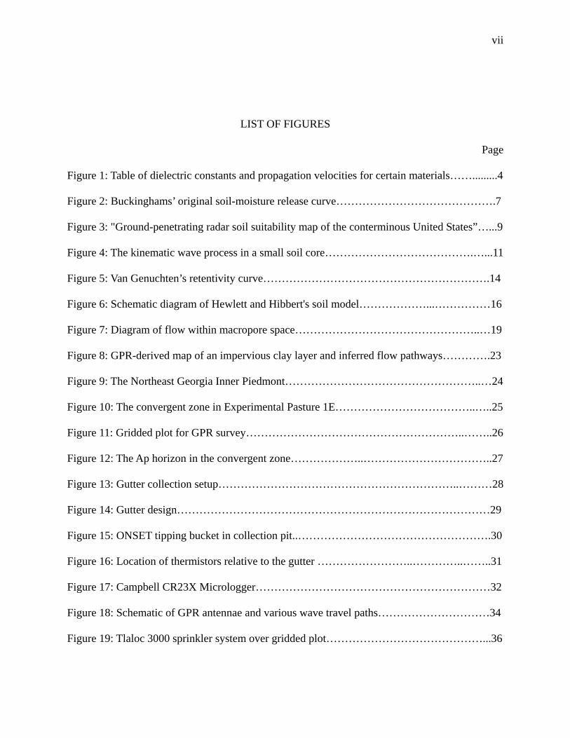
experiment, pressure waves were propagated downwards through a soil core (Figure 4). It was

observed that the wave travelled much faster than the chloride tracer used as comparison. The

experiment was then taken to the field. It was observed that rainfall on the Moore initiated a

pressure wave that travelled laterally down the hillslope. The kinematic contributing area was

found to be approximately 65% of the catchment area. Results from both experiments agreed

with kinematic wave theory: both translatory flow and macropores offer rapid transport.

11

Figure 4. The kinematic wave process in a small soil core (Williams, et al, 2002)

Torres found consistent discharge due to a kinematic pressure wave in his investigations

(Torres, 2002). In the absence of macropores or any other mechanism for preferential flow, a

pressure wave may drive flow if the conditions are correct. When translatory flow occurs water

is displaced rather than released. This displacement does not garner sufficient energy to activate

channels for the initiation of preferential pathways. The mechanism discussed is a threshold

value. When a brief high-intensity burst of rain occurs on wetted soil that is near the threshold

pressure head a slight pressure head increase may occur. The inverse response to this pressure

head increase is a large increase in hydraulic conductivity (K). This response, in turn, forces the

“old water” or soil water downslope. Near-zero pressure heads and had been observed in many

field studies along with concomitant rapid discharge response.

McKinnon discovered that through the stable isotopic analysis of large storm events,

discharge primarily consisted of pre-event, or “old”, water (McKinnon, 2006). It was found that

flow underwent rapid mobilization in a manner consistent with the pressure wave mechanism. A

lag time due to the initial wetting of the slope was observed; this was due in large part to

12

whatever antecedent moisture conditions were present in the soil prior to the event. As with

Rasmussen, et al, perturbations in the subsurface initiated by precipitation is observed as soil

pressures fluctuate creating pressure waves. The initial cause for this was water being pushed

through the system due to the impact of rain on the hillslope surface. The effect is translatory

with water being forced from subsurface zones of antecedent moisture into the gutters.

In many respects the work described herein is a follow-up to both McKinnon's

investigations as well as the subsequent research by Thomas (Thomas, 2009). As in McKinnon's

analysis it was found that gutter responded directly to rainfall. Again a lag time was observed as

the soil needed to be “primed” in order for gutter-flow to be initiated. Another observation in

Thomas' investigation: when the soil is dry and high-intensity rainfall occurs uniform infiltration

does not occur. Non-uniform unstable fronts occur throughout the soil and a preferential flow

called “fingering” occurs. Regardless, the kinematic response mechanism drives pressure wave

translatory flow to cause water to flow laterally into the gutters particularly during dry

conditions. Thomas found that, in addition to the aforementioned pressure wave flow, fingering

caused unstable, uneven flow fronts to occur within dry soil.

Soil-moisture retentivity

Numerical models that approximate fluid flow and transport in the unsaturated zone have

been widely developed. Van Genuchten found some of these methods problematic particularly

“when applied to nonhomogeneous soils in multidimensional unsaturated flow models” (Van

Genuchten, 1980). Closed-form models that predicted the unsaturated conductivity, such as that

developed by Brooks and Corey were seen to be more accurate (Brooks and Corey, 1964).

Nevertheless noticeable discontinuities continued to take place in the slope of the soil-water

retention curve as well as in the unsaturated hydraulic conductivity curve. This occurred at some

13

negative pressure called the bubbling pressure. The discontinuity prevented convergence of

saturated-unsaturated flow problems. The author found that an approach used by Mualem

(Mualem, 1976) suited the need to overcome this problem. Mualem purported an integral

formula for the unsaturated hydraulic conductivity that could enable one to derive closed-form

analytical expressions. It was found that appropriate equations for the soil-water retention curve

were required.

Van Genuchten set about to derive the necessary terms to correct the problem posed by

Mualem's determinations. He formulated a continuous soil-water retention curve of continuous

slope (Figure 5). He utilized Mualem’s equation for predicting the relative hydraulic

conductivity using the soil-water retention curve in which the pressure head is a function of the

dimensionless water content. To solve this equation an expression of the dimensionless water

content was required that related to the pressure head. To this end the author developed a class of

equations based on one general equation. This equation set the dimensionless water content equal

to an expression to the power of “m”. The expression contained by m was, one over one plus the

pressure head times a factor “a”, to the “n” power. In this context a, m and n are fitting

parameters. Through substitution and derivation the author proved that the general form of the

equation could be used to formulate solutions to relative hydraulic conductivity and soil-water

diffusivity. He also discussed the fitting parameters as well as their utilization.

14

Figure 5. Van Genuchten’s retentivity curve The author also obtained similar results in using an equation by Burdine (1953):

conductivity as a function of the dimensionless water content (theta) equal to a complex integral

with theta as the upper bound. The author then proceeded to invert his own general form

equation and substitute it into Burdine’s equation. This resulted in a series of derivations that, as

with earlier derivations, could be used to determine relative hydraulic conductivity as well as

soil-water diffusivity. In the following graphical analysis of his determinations the author found

that the derivations based on Mualem’s equations were more accurate. For this reason the author

chose to cease discussing the Burdine derivations further and only concentrated on his work with

Mualem’s determinations.

In the next section Van Genuchten compared his findings to the Brooks and Corey (1964)

model. Brooks and Corey’s general form consisted of the pressure head over the bubbling

pressure, this expression to the power of negative gamma, all equal to theta. Negative gamma

was an as-yet undefined soil characteristic parameter. The author found that the two models

15

deviated considerably when theta approached saturation. It was also found that the diffusivity

curves were markedly different at intermediate and greater values of the water content. Towards

the end of the paper the author compared actual field data to fitted data and found that, with

some exceptions his models were in good agreement.

Contributions to runoff

The concept of a variable source area was initially discussed by Hewlett in accordance

with experiments that he conducted at the Coweeta Hydrologic Laboratory in 1961 (Hewlett,

1961). The variable source area is a portion of a watershed that contributes to runoff. This area

expands and contracts over time. Research was conducted in order to test the theory that lengthy

soil moisture drainage sustains mountain streams. In studying these mountain streams it was

determined that very little overland flow contributed to perennial streamflow in the characteristic

deep, friable soil of the study area in North Carolina. Due to previous experience Hewlett

determined that bodies of groundwater were restricted to narrow zones along stream channels.

Since an aquifer did not supply these perennial streams with an adequate supply of water it was

surmised that another mechanism must have been present. The unsaturated material, soil had to

be the source for storage and baseflow, since saturated storage was far beneath the stream-base.

Moisture content and drainage are directly proportional, inclusive of soil depth and physical

properties. To test his theories Hewlett constructed an artificial soil profile along a 40 % slope

(Figure 6). It was found that various contributions to hillslope flow could be calculated through a

series of differential expressions. As precipitation, and thus recharge, increased it was observed

that the extent of the contributing areas varied as well.

16

Figure 6. Schematic diagram of Hewlett and Hibbert's soil model A large field area near Stanford University in California was used to determine surface

and subsurface storm runoff processes, each approach to be utilized independently of the others

(Pilgrim, et al, 1978). Initially the common anisotropic and heterogeneous conditions of soil are

discussed as supporting the variable source area concept: interflow, antecedent moisture,

precipitation, duration, etc. Observed in this experiment were: “Horton-type surface runoff,

saturated overland flow and rapid subsurface interflow.” The site was one of a uniform soil type

“Gaviota Loam and Altamont Clay” with a slope of 30% chosen to clearly observe interflow. The

dimensions of the site were 18.3 x 48.4 m. Tracer measurements were used for data collection as

were two sets of collecting troughs located at two “benches”: one bench set at about 27 m

downslope and the other set at the end of the site near a creek. This method, the use of troughs or

“gutters”, is a robust tool for control over flow downslope. Utilizing such means one can monitor

and even control the volume, velocity and dissolved constituents of groundwater in the field.

17

Two natural storms were utilized at the experimental site yet neither produced enough

volume for the utilization of tracers. During the dry season (May, 1968) artificial rainfall was

used for the tracer experiment. 178 mm of water was applied to the entire site using sprinklers at

a rate of 10.7 mm/h. Few instruments were used and the water was collected manually; in fact

nearly all of the work was done manually. Dissolved and un-dissolved organic and inorganic

loads were also determined within the collected water at several times during the experiment.

Each collecting tray was set at different elevations within the exposed soil faces. Subsurface

outflow was seen just above a lower confining silty clay horizon indicating the attenuation of

downward flow due to the lower hydraulic conductivity. Variability in soil type was noted and a

hydrograph was drawn-up for the entire system concerning the later storm. Rapid response to a

storm is noted within the system which supports later findings on the dynamics of the variable

source area. Suspended load response is also noted in this paper. The authors concluded that even

within a seemingly uniform natural system, the variability of hydrological response can be great,

something which they concluded in their findings. The overall response to the storms, both

natural and artificial, was seen as a flushing effect of rapid response through macropores.

Contributions to runoff were found to be extensive and far beyond the field plot.

Preferential flow due to macropores

Subsurface flow can either be described as steady accumulation approaching saturation or

intermittent unsaturated flow (Bouma, 1981). Unsaturated flow is analogous to a “short-

circuiting” effect as water enters dry or unsaturated pores. Pore size is less important than the

continuity of pore interconnection. Four procedures determine macropore flow: field descriptors,

use of schematized, use of staining techniques to characterize macrostructure, and use of

pedological features to determine macropore structure. Previous macropore descriptors are

18

covered with an emphasis on chloride-tracer breakthrough curves for soil structure. Two case

studies are considered: one of infiltration into clay soil with continuous macropores, and upward

fluxes in clay soils. Micromorphology is discussed which is essentially an examination of soil

structure in thin-section using microscopy. In this manner the presence of macropore

development is clearly observed. How these structures are interconnected in situ may be the next

question. How would one go about observing these structures in the field?

Beven and Germann discussed macropores using several different criteria (Beven and

Germann, 1982). One of the most common methods of addressing development has been in

interpreting the soil moisture retentivity curve through pore size classes. Through this method an

analogy is made between the macroscopic retentivity and capillarity of the soil. The overall

change in hydraulic conductivity of the soil may be an indicator of macropore development.

Several types of pores are discussed in this paper such as those formed by: fauna, floral roots,

cracks and fissures due to clay and mineral desiccation, and soil pipes due to natural erosive

processes. Continuity or connectivity is not always a given in the case of these structures.

Difficulties in examining macroporosity are discussed such as the problem of establishing an

equilibrium tension throughout a given sample. When such is the case direct measure of the

macropores themselves are often not available, nor is the exact nature of flow. Experimental

evidence indicated that micropores and macropores at the surface fed lateral macropore flow

once significant flow downward had occurred (Figure 7). The authors summarize that a variable

zone of saturation or a relatively impermeable horizon dominates lateral macropore flows during

subsurface stormflows in the unsaturated zone.

19

Figure 7. Diagram of flow within macropore space (Beven and Germann, 1982). Although macropores (pores larger than 1 mm in diameter yet often not much larger) can

transmit a significant amount of water, mesopores were found to be capable of transmission as

well (Luxmoore, et al, 1990). Mesopores are pores that are smaller than 1 mm diameter. While

smaller than macropores, mesopores have a much higher surface area than macropores. Using

chemical tracers Luxmoore and others determined that mesopore flow path lengths changed in

proportion to stages in the subsurface hydrograph. Macropores were viewed as being important

conduits in zones of physical convergence. The authors determined that a few large

interconnected macropores can have a significant influence on discharge.

In a recent paper the degree of subsurface soil erosion was postulated as one of the causes

of preferential flow (Nieber and Sidle, 2010). Preferential flow was seen as a “self-organization”

process which leads to flowpath connectivity regardless of macropores. The preferential flow

network expands as saturation due to an external flux increases. Regarding these structures, there

may be a lack of connectivity but large localized hydraulic gradients can overcome this. Finite

element models were utilized in determining flow through hypothetical blocks of soil, both with

and without macropores. Macropores containing coarser grained materials directly influenced

flow through the soil block. As the application of precipitation increased the outflow increased in

20

a like manner due to the influence of macropores. These structures were also seen as producing a

variance of flow versus the soil blocks that did not contain them. Flow in the domain without

macropores was found to be very regular while occurring yet that flow was seen as

discontinuous. Small-scale erosion within the pores themselves guided connectivity: flow

occurred within a series of flowpaths in the most energy-efficient manner possible. The

increasing connectivity of volumes of soil moisture was the key to establishing preferential

flowpaths in the model. Macropore development exacerbated the process. They are essentially a

mechanism for increasing the velocity of flow as well as the direction of flow, to a certain extent.

Ground-penetrating radar utilization

Radar waves are of sufficiently high frequency to travel through earth materials unimpeded

with little dispersion (Sharma, 1997). The relative permittivity or dielectric constant of materials

controls the velocity of radar waves through them. The dielectric constant is the ratio of the

dielectric permittivity of the medium to the dielectric permittivity of free space. The dielectric

permittivity is the electrical displacement or polarization property of materials that normally

behave like insulators. High frequencies, such as those emitted by radar, enable such materials to

behave like conductors. When these electromagnetic pulses encounter differential dielectric

constants they are, in part, reflected. The intensity and amount of the reflected signal is dependent

on the dielectric contrasts between layers as well as thickness of the layers encountered. Thicker

layers tend to attenuate the signal as does an increase in depth. The velocity of radar waves within

earth materials is based on the ratio of the speed of light over the square root of the permittivity of

free space times the materials dielectric constant. Since the dielectric permittivity of free space is

close to unity (unless highly magnetic materials are involved) this value is generally not used. Thus

the velocity of a signal is highly controlled by the dielectric constant.

21

GPR has been used in geophysical, hydrological and soil surveying for well over 40

years. Some of the earliest work in the hydrological applications of standard pulsed radar (not

GPR) was conducted by the U.S. Army Corps of Engineers for the Mobility Environmental

Research Study (MERS) (Davis, et al, 1966). Soil samples were prepared at varying soil

moisture contents. Standard pulsed radar signals of 297, 5870, and 9375 megacycles per second

(analogous to megahertz) were directed into the soil. Unlike future attempts (current GPR

antennas are placed directly on the soil) the radar antennae were set above the surface of the soil

at a height of approximately 15 feet above the sample, at varying angles incident to the surface of

a given soil sample. Despite this fact the authors reported a robust moisture value for a

homogeneous soil. It must be noted that the standard pulsed radar systems that were used in this

study were amplitude sensitive only. Signals were indicators of surface water and homogenous

soil moisture content due to the dielectric constants determined reflectance values. It was also

determined that the electrical properties of the soils were concomitant with soil moisture values.

It was surmised through analysis of the returns that longer radar waves (within 225-390 MHz)

could be used to determine some depth values including those of a given water table. It must be

kept in mind that throughout this study the radar signal was sent into the soil from above the soil

itself. Current GPR technologies apply the antenna and receiver directly onto the soil.

In a paper by Doolittle and Collins (1995) the authors presented an overview of use for

GPR in soil survey work. GPR is a powerful tool for delineating the often abrupt transitions from

one soil profile to another, something that may not be apparent from a surface examination. Soil

horizon interfaces often produce strong radar reflections. Listed are the many additional

pedological uses for GPR: depth to hardpans, dense till and permafrost; color inference; organic

carbon content; organic materials determination; depth to shallow water table in coarse textured

22

soils; assessment of lamellae or cemented layers; evaluating layer or horizon thickness; and uses

in forestry applications. GPR is also a versatile and robust tool for use in the creation of soil

maps. In addition GPR provides a quick and efficient method of conducting soil surveys: both

cost effective and non-destructive. The author points out that this method is not perfect though

and soils of high conductance limit its use: it is not useful on certain kinds of soils. Use is

frequency dependent with higher frequencies (> 500 MHz) being better utilized for shallow field

work for higher resolution. In contrast lower frequencies, with longer wavelengths, provide good

support for deeper imaging albeit with a lower resolution. Soil factors affecting conductivity are:

porosity and water saturation (water being a good electrical conductor), salt content in solution

with a higher proportion of ions at exchange sites, clay content with 1:1 (kaolinitic) clays as

being more favorable, and scattering which is a function of soil texture.

A 2002 GPR investigation in sandy soil confirmed the use of GPR as a robust method for

determining soil-water and flowpaths (Gish, et al, 2002). In conjunction with soil-moisture data

the survey which took place in Beltsville, MD confirmed accurate identification of flowpaths.

Different layers of soil were identified as being either restrictive or conductive. Those layers of

conductivity were within the upper sandy soil layers for the most part. The authors summarized

that soil-moisture data with an adherent GPR survey had the following qualities: this type of

investigation could “be an effective tool for evaluating and monitoring sub-surface flow

processes”, “the spatial location of the soil moisture monitoring system is critical to monitoring

water movement”, and “real-time monitoring of water movement is critical if preferential flow

pathways are to be accurately monitored.” It must be kept in mind that the area covered for this

particular survey was 350 by 300 m. A survey on such as scale is generally not going to identify

23

flowpaths on a very fine-scale. Specific zones of macropore activity were not resolved although

GIS data was used to indicate the possible location of flowpaths in plan view.

Gish and others recently proposed a method to identify sub-surface pathways utilizing

GPR, digital elevation models and soil-moisture data (Gish, et al, 2005). The study site covered

an area of 3.2 hectares (32,000 m2). Since utilizing GPR over such a large area is usually an

unrealistic proposition radar surveys were made only at discrete locations. The locations of

flowpaths were inferred through the use GPR as well as the other methods utilized. An elevation

map of an impervious clay sub-layer was produced using such a method (Figure 8). Flow

pathways were inferred using the various datasets but not specifically identified.

Figure 8. GPR-derived map of an impervious clay layer and inferred flow pathways

24

CHAPTER 3

SITE DESCRIPTION

Overview

The area of investigation was on at the United States Department of Agriculture

Agricultural Research Station (USDA-ARS) J. Phil Campbell Senior Natural Resource

Conservation Center in Watkinsville, Georgia (N 33º54’, W 83º24’) in the Inner Piedmont

Physiographic Province of North Georgia. The site is within agricultural pasture, a footslope in

the East Unit of USDA-ARS property on Experimental Pasture 1E (Thomas, 2009).

Figure 9. The Northeast Georgia Inner Piedmont (McKinnon, 2006)

25

The test site used for collecting data is in a topographic convergent hillslope zone (Figure

10). The topographic convergence creates a distinct trough shape in this part of the slope. The

soil in this area is of the Cecil series: an Ultisol. These soils feature a distinct Bt horizon.

The parallel zone to the right of the convergent zone, as one faces uphill, was not utilized

for this study; neither was the left side of the convergent zone. All of these zones were utilized in

previous studies (McKinnon, 2006; Thomas, 2009). Both the convergent zone and the parallel

zone were infrequently monitored from winter of 2008 through the spring of 2010. This was to

monitor for natural conditions as well as testing and maintaining the site. A large body of

continuous monitoring data was made available for this work from previous studies conducted in

the area by McKinnon and Thomas.

Figure 10. The convergent zone in Experimental Pasture 1E The site utilized for the GPR experiment was on the right-side of the hillslope as one

looked uphill, a site referred to as the convergent zone. This plot sits atop a slope within the site

that is naturally shaped in such a manner that flow tends to converge with reference to the

relationship between the left and the right hand sides of the slope. The left side of the convergent

26

zone was not utilized in this experiment other than for the obtainment of soil core samples for

use in a laboratory experiment. Directly above the gutter system on the right hand side of the

slope a 280 x 200 cm grid made of twine was assembled (Figure 11). Twine is a material that is

“invisible” to GPR. The space of each grid was 10 x 10 cm. This 56,000 cm2 area was where

artificial precipitation was induced for the artificial rainfall experiment.

Figure 11. Gridded plot for GPR survey

Climate

The climate at USDA-ARS is typical of this part of the Southeastern United States. The

air quality is normally quite humid and the mean annual rainfall is 125.2 cm (Endale, et al,

2002). Mean monthly rainfall is highest (11.5 to 14.0 cm) during the winter months, and least

(7.7 to 8.6 cm) in the fall. Average daily temperature ranges from 23.9˚ C to 26.7˚ C in June–

August (summer months) to 4.4˚ C to 7.2˚ C in December–February (winter months).

Soil

27

The soil at the experiment site was in the Cecil series, an Ultisol: clayey, kaolinitic,

thermic, Typic Kanhapudult. Soil genesis originated in the feldspathic biotite gneiss basement

with a minor component of granitic lithology. The soil is generally well-drained with moderate

permeability. It contains a high amount of kaolin clay. The clay content is highest in the Bt-

horizons. The Ap-horizon tends to be loamy with a high sand content (2007, Franklin, et al). A

textural analysis of the soil in this area resulted in a particle size distribution of: 70.3 % sand,

3.16 % clay and 26.54 % silt (sandy loam) (McKinnon, 2006). The soil horizon is of interest was

the Ap where the drip plates were installed at 10 cm (Figure 12).

Figure 12. The Ap horizon in the convergent zone

28

CHAPTER 4

METHODS

Overview

There were two subsequent experiments conducted using the rainfall/sprinkler system in

conjunction with the gridded plot and a runoff gutter collection system. The first experiment is

the one discussed in this paper: the radar survey. Immediately after the GPR survey was

completed a conservative tracer experiment was conducted on the same grid by Beasley

(Beasley, 2011). Both the results from this paper and the research conducted by Beasley are

ultimately part of the same overall investigation of hillslope processes and groundwater delivery,

and can ultimately be seen as two parts of a complete picture regarding these processes.

Figure 13. Gutter collection setup

Gutter and data collection system

A gutter system had previously been installed on each hillslope. Both the parallel and the

convergent zones featured trenches dug perpendicular to the slope. The dimensions of these

trenches were 1.45 m lengthwise with a depth of about 0.1 m, on average (Figure 13). There

29

were two such systems set-up, two gutters in the parallel zone and two in the convergent zone.

As previously mentioned only one gutter was utilized, the right-hand gutter in the convergent

zone. Within these trenches a metal gutter was in place that served to intercept subsurface runoff

that occurred at the upper boundary (Figure 14).

Figure 14. Gutter design (McKinnon, 2006) A large wooden board as well as non-conductive clay was used to prevent any overland

flow from entering the system while precipitation occurred. In addition to this plastic tubing was

installed to siphon away water that tended to pond up on the steep and uneven slope of the field

plot. The only water that entered the gutter was water that flowed from the vertical cut face

directly over the gutter. Seepage plates were installed approximately 10 cm below the surface in

accordance with previous studies (McKinnon, 2006; Thomas, 2009). These were so placed as to

allow flow to concentrate at one end which is at a slightly lower elevation. The part of the gutter

that was at a lower elevation had an opening that was attached to a tube. The tube was buried

30

under the soil, ending-up in a small collection pit that contained an ONSET1 tipping bucket rain

gauge (Figure 15). The ONSET unit would release the water into another tube under the plastic

bucket that demarcated the pit. The tipping bucket held 0.254 cm of rain per tip before it released

it downward under the bucket, through the tube and downslope away from the site. Each “tip”

would count as one volume of water, which could be stored as information for later use.

Figure 15. ONSET tipping bucket in collection pit (Thomas, 2009) The trench as aligned along a contour line, a line of equal elevation. The series of drip

plates aided in inducing flow. As response occurred water flowed over the drip plates into the

gutter. The gutter, angled slightly downslope towards the left was attached to a tube and this

water would flow into the ONSET tipping bucket downslope. The tipping bucket was installed in

a small pit downslope from the grid-plot. This water was recorded as tips that flowed in volumes

of 0.254 cm. Each tip registered as a count with a Campbell CR23X Micrologger that was

hardwired to the ONSET unit (Figure 17).

1 Onset Computer Corporation, MacArthur Blvd., Bourne, MA 02532

31

Originally the ONSET unit was set to record tipping data within its internal memory but

this feature malfunctioned and no tipping data was recorded before 6/9/2010. To correct this, the

Micrologger was programmed to record tipping data on 6/9. The Micrologger was hard-wired to

the ONSET tipping bucket to do this. The Micrologger was programmed to record continuous

temperature data from three thermistors as well as tipping bucket data. One thermistor was

placed vertically in the ground at the bottom of the grid (T1, which corresponded to the

southwestern portion of the grid), another was placed approximately 10 cm to the left of the

leftmost seepage plate (T2), and the third one was placed in the gutter itself near the exit spout

on the left (T3) (Figure 16).

Figure 16. Location of thermistors relative to the gutter Once the small bucket tipped over it would deliver the “cast-off” to a tube under the

tipping bucket that lead to a containment vessel at the bottom of the slope which was periodically

emptied. The Micrologger would record the clicks as counts over the period of time that the

experiment took place in (Figure 17). Such systems are often used to accurately determine

precipitation of a period.

In addition to the runoff data from the tipping bucket rain gauge the Campbell unit was

used to record soil temperature changes throughout the experiment duration. Thermisters were

32

installed into the hillslope at the gutter: one vertically in the soil above the gutter, one

horizontally into the soil to the left of the gutter, and one within the gutter itself. Differences

between the gutter water and the soil profile could be observed with these instruments. The

results were extracted from the Micrologger after the experiment (Figure 17).

Figure 17. Campbell CR23X Micrologger

A simple rain gauge was installed at the top edge of the grid in order to record hourly

rainfall volumes above-ground. This gauge was emptied periodically in order for the rainfall

levels to continue being assessed accurately. Final readings were averaged on an hourly basis.

Plot-scale ground-penetrating radar

The GPR runs were conducted over a 5.6 m2 area of the convergent zone directly above

and adjacent to the gutter. Artificial rainfall was applied to the soil for various periods of time,

usually two to three hours. The 280 x 200 cm2 area was subdivided into 10 x 10 cm squares for

33

use in observing specific areas. This grid was constructed using twine, a “radar-opaque” material

that was attached to long nails outside of the area of GPR utilization. This enabled for the

operation of the GPR antennae in 10 cm increments. A test run was made with a 900 MHz GPR

antennae five days before the main experiment. Initially the intent was to use a 2600 MHz GPR

antenna but in testing the antenna it was revealed as incompatible with the SIR-2000 control unit.

Consequently a GSSI 1500 MHz antenna would be used for the experiment.

The GPR unit and antenna utilized for this experiment were somewhat typical for these

types of instruments. The control unit generates electromagnetic waves in the radar frequencies.

The antenna unit serves as both transmitter and receiver for these waves once they are reflected

back up to the surface (Figure 18). The antenna is towed over the ground surface at a steady rate

as the signal is sent down into the subsurface (Figure 20). Returns are reflected upwards due to

the differential properties of the subsurface materials, the differential dielectric constants of the

various materials. This particular antenna, as is the case with many such units, was shielded from

interference by objects external to area of interest.

When radar waves encounter a contrast in dielectric constants below the surface they are

reflected back to the surface due to the reflection coefficient of the dielectric values (Lunt, et al,

2005). This is the square root of each dielectric constant used in ratio: the ratio of the upper value

minus the lower value, above the upper value plus the lower value. Higher differential dielectric

contrasts generally produce greater amplitudes of return. When radar waves are transmitted there

are three components present: the above-ground airwave, the groundwave that is slightly below

the surface and the reflected wave making up most of the electromagnetic energy (Figure 18).

Before any survey is run the unit is put through a few tests to determine the location of the radius

of the reflected wave; this known as the Fresnel Zone. The GPR control unit, in this case the

34

SIR-2000, is adjusted to record only the radar waves that are within the Fresnel Zone. The

above-surface airwave and the near surface groundwave, both sources of noise, are not regarded

in this respect.

When the unit was initially adjusted several gain points needed to be set. These are values

that allow the signal to stay within a range that would eliminate high gain distortion. For the

entire survey a range of five was used with five corresponding gains: 8, 18, 30, 34 and 34. The

position of the center frequency was set to 100 nanoseconds (ns) downward. The radar unit

emitted the antenna value as the center frequency, which was 1500 MHz.

Figure 18. Schematic of GPR antennae and various wave travel paths (Lunt, et al, 2005)

Ground-penetrating radar survey timeline

The GPR system utilized a SIR-2000 control system for radar monitoring and data

collection. An initial survey was conducted for calibration purposes on June 2 using a 900 MHz

antenna. An attempt was made to utilize a 2600 MHz antenna for the experiment but this was

abandoned due systems incompatibility. It was decided that a 1500 MHz antenna would be

utilized because that is suitable for the SIR-2000. That particular antenna would, in theory,

provide a greater resolution of the subsurface. The GPR survey for the experiment documented

here began on June 7, 2010 at 1338 EDT and concluded June 16 at 2146 EDT (Appendix A).

The various components of GPR used for this survey are as follows: the GSSI SIR-2000

control unit, shielded coaxial cables connecting the SIR-2000 control unit to the antenna, the

35

1500 MHz shielded antenna unit and a 12-volt battery which ran the unit. The surveys were

conducted by hand as the antenna operator dragged the unit across the ground surface and the

control operator monitored the SIR-2000 control unit. The control operator would initialize

transmission and “call” to the antenna operator to begin steadily dragging the antenna over the

ground surface over the length of the survey. Once the end of the line (literally since twine was

used) was reached the antenna operator would call out to the control operator who would stop

transmission of the radar signal. Every survey was conducted in this manner.

A total of 15 surveys were conducted over this period of time. 14 of those surveys are

documented here. The last survey was somewhat incomplete as the entire 5.6 m2 was not utilized

for it; it has been omitted from the dataset. The first survey was taken over dry ground since the

prevailing weather conditions at the time were hot with temperatures averaging 29.5° C. Hot dry

days often give way to afternoon and evening thundershowers in the Northeast Georgia

Piedmont; during the experiment these conditions prevailed. At least twice during the afternoon

the survey had to be abandoned for the day due to thunderstorms. The GPR unit was not operated

during rainfalls: the control unit could have been damaged had water entered the chassis.

After the initial survey each GPR run was conducted after periods of wetting. A Tlaloc

3000 sprinkler system wet the soil surface with ~7.6 cm of rain per hour (Figure 19). Wetting

would take place for two to three hours initially but once a response occurred on June 11 at 1524

EDT the periods of wetting were conducted for only 30 minutes or so. This is because once the

system was “primed” it would respond to perturbations in pressure. Wind conditions were mostly

calm with tarps used when wind velocities increased.

36

Figure 19. Tlaloc 3000 sprinkler system over gridded plot

Between periods of wetting the SIR-2000 unit was assembled from a stand-by position

and a GPR survey was conducted. This took anywhere from 15 to 25 minutes. Then, one

operator monitored the SIR-2000 control unit and the other operator dragged the attached radar

antenna along the ground (Figure 20). The operator behind the control unit would “call” when

the radar was activated and then the antenna operator would drag the antenna across the grid,

along the twine that demarcated the 10 cm x 10 cm “cells”.

Once that particular transect was completed the operators would complete that particular

survey. Although the antenna emits a signal the roughly spreads 120º outwards each transect is

considered to be a two dimensional “slice” into the ground, length-wise and depth-wise. Each

survey consisted of a “y-run” conducted upslope within the gridded area and an “x-run”

conducted perpendicular to the slope. Doing GPR surveys in such a manner assures complete

coverage as well as the elimination of outlying, anomalous data. This is the reason that the metal

drip plates along the bottom of the plot did not interfere with radar returns. An orthogonal (x,y)

37

survey eliminates “side-swipe” which is where the second lobe of the radar signal picks-up

anomalous elements.

For each walk the antenna was dragged along the ground following lines spaced 10 cm

apart. The SIR-2000 unit saved the information from each run into its internal memory. This data

could later be extracted and saved onto a computer hard-drive.

Figure 20. Antenna operation for GPR survey

These radar returns were created from files saved in the SIR-2000 control unit in the

field. The files were saved within the control unit then converted into .dzt format files for

transfer into a computer. Then these files were converted to .dat files which were used to

generate .jpg files. The results were the images used in analysis. The .dat files contained

frequency and intensity of return information as well as the Cartesian coordinates of these

values. These files are extremely useful in numerically analyzing the radar returns.

38

Tempe cell experiment

Soil for the Tempe cell experiment was taken from the unused left gutter in the

convergent zone approximately one meter to the left of the right-hand gutter used in the

experiment. This was done on June 29, eight days before the artificial rainfall experiment. To

obtain a sample for use in the Tempe cell array 3.5 in (8.89 cm) diameter brass cylinders 2.36 in

(6 cm) deep are carefully hammered into the soil using a rubber mallet. The core is then

extracted from the soil face. The intact soil core is wrapped in cheesecloth and transported to the

laboratory. Five cores were taken from ARS for analysis in the laboratory with Tempe cells.

Figure 21. Typical Tempe cell array (University of Georgia Soil Physics Laboratory)

The Tempe cell experiment took place from June 24 to July 7, 2010 in the Forest Soils

Laboratory at The Warnell School of Forest Resources on the University of Georgia campus. A

Soilmoisture Products 1400 Tempe cell array was used to obtain data for a retentivity curve

(volumetric moisture (θm) content versus matric potential (Ψ)). The Tempe cell experiment

consisted of a series of small pressure chambers housing the soil samples (Figure 21). The basic

assembly is made up of of a cylinder containing the soil core placed atop a porous ceramic plate.

This is clamped together tightly using a housing assembly with several rubber rings between the

39

brass cylinders and the plates. This is to keep the unit sealed airtight. The cylinders are then

placed within a manifold. Fed into each assembly is a tube that originates from a pressure gauge.

This pressure gauge is connected to a hose that constantly supplies air. Each stage of the Tempe

cell experiment is fed air at discrete pressure intervals. As the air pressure is incrementally

increased water is forced out the chamber through the ceramic plate. For this experiment the

pressure was initially set at 0.2 bars (20,000 Pascals) with increments of 0.2 bar adjustments

made throughout the experiment. The maximum pressure set was one bar after which the

experiment was terminated. Throughout the experiment the massed of the core samples were

measured in order to assess the volume of water that had been drained out of the soil samples.

40

CHAPTER 5

DATA AND RESULTS

Ground-penetrating radar returns

Changes in soil-moisture content were made visible through radar returns. These were

“snap-shots” of moisture content sometime after the sprinkler was shut-off. Actual water

movement was not visualized since it took several minutes to assemble the GPR survey after

each period of wetting. By the time the survey began the water had drained out of the soil. Thus

the returns present images of residual moisture.

The radar returns indicate changes in the soil moisture content due, in turn, to changes in

dielectric values. Some zones in the soil are seen to have higher dielectric values, moisture

increases, while others have been “emptied-out” showing low values. These values are strongly

constrained by water or moisture-content: the dielectric constant of water is ~81 for free-standing

freshwater.

A series of 930 individual radar surveys along transect took place throughout the GPR

field experiment. These surveys were conducted over the 10 x 10 cm transect grids. The last

survey which comprised 38 different returns was incomplete and is not used in this study. The

892 surveys utilized here record returns at discrete depths noted on the return images. The

surveys, conducted along intersecting perpendicular transects, are interpolated into plan-view

images utilizing GPR-Slice v.7.0 software2. A total of 48 different discrete plan-view images

were generated for 48 different depths. There were 14 total utilized surveys conducted in the

2 Dean Goodman, Geophysicist PhD, Geophysical Archaeometry Laboratory, 5023 North Parkway Calabasas, Calabasas, California 91302

41

field and of these there were 672 plan view images generated. Each of the 14 surveys generated

48 plan views for 48 different depth images.

A depth for Survey L, first gutter-response, was generated using one of the features in

GPR-Slice v.7.0. Since each survey was conducted in an identical manner these depths

correspond for all surveys. The lowest depth of survey was 28 cm. Dividing 28 by the number of

intervals, 48, yields a depth of ~0.58 cm per interval. The radar returns show shifting areas of

differing dielectric values in each layer. Each return was consistently color-coded with “warmer”

color values such as red indicating higher intensities of return due to dielectric values. Figure 14

shows higher dielectric values towards the bottom of the grid at depths of ~10-28 cm. As

moisture is moved through the soil profile moisture levels fluctuate as indicated in Figures 22a-

22c. These images represent concurrent depths. Figure 22c features survey L which was taken

immediately after the first, and largest, gutter response.

Figure 22a. Radar return examples from GPR survey A, 6/7/2010, 1338 EDT

42

Figure 22b. Radar return examples from GPR survey I, 6/10/2010, 1409 EDT

Figure 22c. Radar return examples from GPR survey L, 6/13/2010, 1557 EDT

43

Because the rainfall simulator had to be shut-down before each GPR run significant soil

moisture changes may have occurred prior to the survey. This is supported by the observation

that runoff ceased before the GPR could be deployed. It took approximately 10-30 minutes to

deploy each GPR survey, mostly due to the necessity of carrying the scaffolding up and down the

hill. Gutter-flow using artificial rainfall normally stops about eight minutes after the sprinkler is

shut-down. Thus the resulting image is one of residual soil moisture content.

At 1500 MHz median wet clay will resolve only about 5.5 cm. This constraint on the

resolution of soil-moisture results in broad patterns of soil moisture made visible. Any flowpaths

or structures smaller than about 5.5 cm are “bundled together”. Implied resolution can be derived

using the formula for spatial resolution as an inverse of the median radar signal frequency times

the square root of the dielectric constant.

Micrologger data

In Figure 23, the corresponding thermistor data reads a as follows: T1 was placed

vertically in the soil about 5 cm above left side of the gutter, T2 was set about 10 cm below the

soil surface horizontally placed in the soil about 5 cm to the left of the gutter, and T3 was placed

in the gutter itself on the left-hand side just before the downspout attached to the tubing (see also

Figure 16). The flow data is labeled “Q” in the key to the right of the chart and represents tips in

the rain gauge at a volume 0.254 cm per tip.

Also all of the flow data before 6/10/2010 will not be discussed due to overland flow

originating from a breach in the cover system. This was corrected on that day by realigning the

cover board and applying an impermeable clay seal to the board/soil interface. All of the

Micrologger data after 6/13/2010 corresponds to the chemical tracer experiment, not the GPR

survey. Two tipping events (flow data) are covered in this study: 6/11/2010 at 1524 EDT, and

44

6/12/2010 at 1243 EDT. A tipping event occurred on 6/13/2010 overnight and was not associated

with a GPR survey. This event did not occur during the artificial rainfall experiment and will not

be considered here.

One can observe the regular diurnal temperature variation that occurred over the time

period in the Micrologger data (Figure 23). This corresponds well with the marked increases in

afternoon temperatures during the summer months for this region. Thermistor T3 shows the

greatest variation in temperature change. The range for T3 covers ~11º C compared to the ~9º C

for T1 and the ~7º C for T2. A slight drop in T3 occurred during the two tipping events on 6/11

and 6/12.

The initial flow event (Q) which took place before 6/10 was due to overland flow that

leaked through the surface sealing system. This error was corrected shortly afterward. The first

gutter-flow that is considered for this study occurred on 6/11 and recorded about 1000 tips which

was the greatest amount of flow measured during the experiment. Each tip measured 0.254 cm of

rainfall depth. Since the initial gutter-flow was 35 minutes long and produced 1000 tips this is

254 cm of gutter-flow in 35 minutes or 7.257 cm/min. Figure 23 shows the thermistor, gutterflow

(discharge), and rain (artificial precipitation) information as downloaded from the Micrologger

(Figure 23). Included is sprinkler activation (“Sprinkler On”) and run information (designated by

letters at the top of the graph) for correlation. Figure 23 can be correlated with the information in

Appendix A.

45

Figure 23. Thermistor, discharge, rain, sprinkler activation and run information

Soil-moisture retentivity curve

Two retentivity curves, also known as the soil moisture curves were generated based on

the Tempe Cell experiment. A computer program, RETENTIVITY3, was utilized to create these

graphs. Each retentivity curve corresponds to a specific depth modeled for analysis. Figure 24a is

a retentivity curve corresponding to a depth of 0-6 cm and figure 24b is a retentivity curve for 5-

11 cm. This corresponds well with the depth of interest for soil-moisture which is the top 10 cm

or so of soil: an Ap horizon.

The retentivity curve is useful in analyzing a ability to retain moisture: volumetric soil-

moisture content is a function of the soil tension, also known as matric potential. This is roughly

analogous to “negative tension”. This value is a measure of a soils capillarity which is the

measure of soil-water available for uptake by plant roots. As volumetric moisture content 3 John Dowd, UGA Department of Geology, Athens, GA 30602

46

decreases the amount of matric potential increases. This matric potential is a function of the

tension of the water residing within the void space between grains of soil.

Figures 24a and 24b both exhibit a similar characteristic soil-retention “s-shaped curve”.

As one proceeds down the soil column compaction becomes greater as does the clay content.

Thus water is increasingly retained at greater depths. The Ap horizon at ARS is characteristically

well-drained; both figures exhibit this quality. Each curve models a considerable release of water

from an air-intake pressure of 0.2 cm of water to 0.8 cm. The points marked on the curve

represent the actual data from the Tempe Cell experiment. The green line in each curve is the

soil-moisture retention model based on Brooks and Corey and the red line is the Van Genuchten

model (Brooks and Corey, 1964; Van Genuchten, 1980). These are two of the most common

models used to determine soil-water retention. Each determination represents the effective

saturation of a soil as a function of certain pressure changes within the soil.

The Brooks and Corey function was determined based on experimental values; the Van

Genuchten function was empirically derived. As the moisture content of a soil decreases the soil

tension, or matric potential, tends to increase. Each curve was generated using RETENTIVITY

and then adjusted via several parameters to a best fit for the data points.

47

Figure 24a. Soil-moisture retentivity curve, 0-6 cm dept

Figure 24b. Soil-moisture retentivity curve, 5-11 cm depth

Miscellaneous data

The rain gauge was placed in the soil just above the gridded plot. The gauge was set

within the sprinkler systems range of coverage. The rain gauge recorded, on average 7.6 cm of

precipitation per hour at a uniform sprinkler setting of 7.5 pounds per square inch (psi) which is

equivalent to 51,710.68 pascals.

48

Several times during gutter-flow the cover board was lifted up off of the top of the gutter

in order to view the flow out of the 10 cm deep seepage face. It was observed that the water

came forth in pulses rather than as steady outflow. These pulses erupted from discrete zones on

the soil face, not over the entire length. The steadiest and strongest pulses observed occurred on

the left side of the soil face. After the sprinkler was shut-off flow continued for about eight

minutes.

A tracer experiment was conducted from 6/14/2010 to 6/16/2010 directly after the GPR

experiment on the same grid (Beasley, 2011). In this study, areas used for tracer application were

in part determined from the radar returns discussed here.

49

CHAPTER 6

DISCUSSION OF RESULTS

Overview

It has been determined from previous study at the site that runoff from storm

events consists of a great amount of pre-event water (McKinnon, 2006; Thomas, 2009). These

investigations had determined that an aforementioned kinematic pressure wave is one of the

primary means of soil-water movement (Rasmussen, et al, 2000; Williams, et al, 2002; Torres,

2002). This water, rapidly mobilized due to translatory flow, mostly consists of antecedent soil-

moisture. The motion of precipitation striking the soil surface is the initial physical activity that

drives the water through rapid delivery pathways in the soil. As moisture levels in the soil

approach saturation during precipitation a threshold condition for water delivery is reached

within the system. Also when water ponded at the surface the system would shut-off and flow

would cease. The direct action of raindrops on the surface was required for flow to initiate. A

steady “pulse” was observed at discrete zones in the soil face once activation had occurred,

mainly near the left side of the gutter. The impulse of the kinematic pressure wave causes

antecedent moisture to be driven out of pores within the soil profile.

When macropores are present interflow occurs: a lateral process (Nieber and Sidle, 2010).

The mechanism of flow with study was the kinematic process driving old water or antecedent

moisture through macropores into ephemeral channels. The direct resolution of these

macropores, often microscopic in scale, cannot be resolved (Beven and Germann, 1982;

Luxmoore, et al, 1990). As with much of the literature, mainly moisture content remains

detectable by GPR yet the moisture conditions of the soil can also be analyzed using the soil

50

moisture curve which is characteristic of the types of soils found in the research area. This is a

common problem in this field.

The threshold condition for translatory flow occupies a margin between periods of initial

wetting when the soil is “primed” towards near saturated conditions. Once rainfall was shut off

and restarted perturbations occurred within the soil that initiated gutter response. With volumes

connected, possibly via macropores, flow was initiated. Furthermore the flow due to

kinematically-driven subsurface preferential flow behaves like overland runoff with regards to

both high speed and the delivery of large volumes. Artificial rainfall measured ~0.13 cm/min;

runoff response yielded ~7 cm/min. This is ~50 times the amount of runoff to rainfall. This

equates to artificial rainfall of 7.6 cm/hr versus a gutterflow of 435 cm/hr. This far exceeds the

rainfall and indicates a contributing area much larger than the 280 x 200 cm plot.

Resolution of radar signal

Soil moisture as a function of the dielectric constant was analyzed using the following

chart (Figure 25). As can be seen the frequency of 1500 MHz allows for a general resolution of

approximately a wavelength of 5 cm. There is a range to be considered though so this is merely

the median return since 1500 MHz is the center frequency with a range from ~150 to 3000 MHz.

The resolution of radar wavelength is inversely related to the frequency of the antenna with the

center frequency given precedence. Figure 25 is a graph of the functional relation between

resolution and frequency. Since c and ω are both known quantities and assumed to be fixed, the

variables are λ and εr. The resolution (λ) and the dielectric constant (εr) are inversely related,

non-linear functions of each other. That being told there are actually two considerations to be

made when considering “resolution”.

51

Resolution of the radar signal is dependent on the number of datapoints in the area over

which one averages the count value, as opposed to wavelength resolution. As observed in the

output .dat files (which contained the radar return information) the value was one datapoint per

10 cm2. This is much larger than any given macropore or other flowpath structure; in fact

flowpaths are orders of magnitude smaller than the radar returns resolution capabilities. Thus,

while patterns of soil moisture and hydrological responses may infer the activation of flowpaths,

it can be safely assumed that GPR can never resolve individual flowpaths. This is not a

premature assumption. Within the auspices of this research as well as within the literature

hydrological flowpaths continue to be a case for inference. Current technologies and techniques

are incapable of resolving such minute structures so the notion can be dismissed at this point.

Maximum depth of penetration is often somewhat variable using GPR due to varying

dielectric constants and soil heterogeneity. The deepest layer imaged by the GPR-unit is

indicated by the GPR-Slice to be a one nanosecond (ns) interval. This was determined using a tab

in GPR-Slices “Options” menu. The speed of light is 29,979,245,800 cm/s; one ns equal to 10-9 s

which yields approximately 30 cm. As a dielectric constant of 81 is reached the resolution

(wavelength) will asymptotically approach zero (Figure 25).

52

GPR resolution vs. dielectric constant during wetting: 1500 MHz antenna, avg. clay soil

4.000

4.500

5.000

5.500

6.000

6.500

7.000

7.500

8.000

8.500

9.000

9.500

10.000

4.00 5.00 6.00 7.00 8.00 9.00 10.00 11.00 12.00 13.00 14.00 15.00 16.00 17.00 18.00 19.00 20.00

Dielectric constant (εr)

Res

olut

ion

(cm

)

515 εr, 5.16 cm

Wetting increase

Figure 25. Modeled radar resolution as a function of dielectric constant during wetting

Images from radar returns

Through the sequence of GPR returns the priming of the soil can be seen as an increase in

the dielectric values of the soil with brighter, bolder colors used to represent higher values. Soil

moisture is a linear function of the dielectric constant so the wetting of the soil is directly

observed using GPR. Once gutter flow is initiated in profile L the “emptying-out” of volumes

within zones of soil moisture occurs (Figure 26). The replacement moisture values from survey L

to M are zones of high moisture content that replaced zones of low moisture.

53

Figure 26. Returns before (K), immediately after (L) and hours after first response (M)

Throughout the first 11 GPR surveys (A through K) no water was seen flowing out of the

gutter soil face. For each of these GPR runs the sprinkler system was run almost continuously

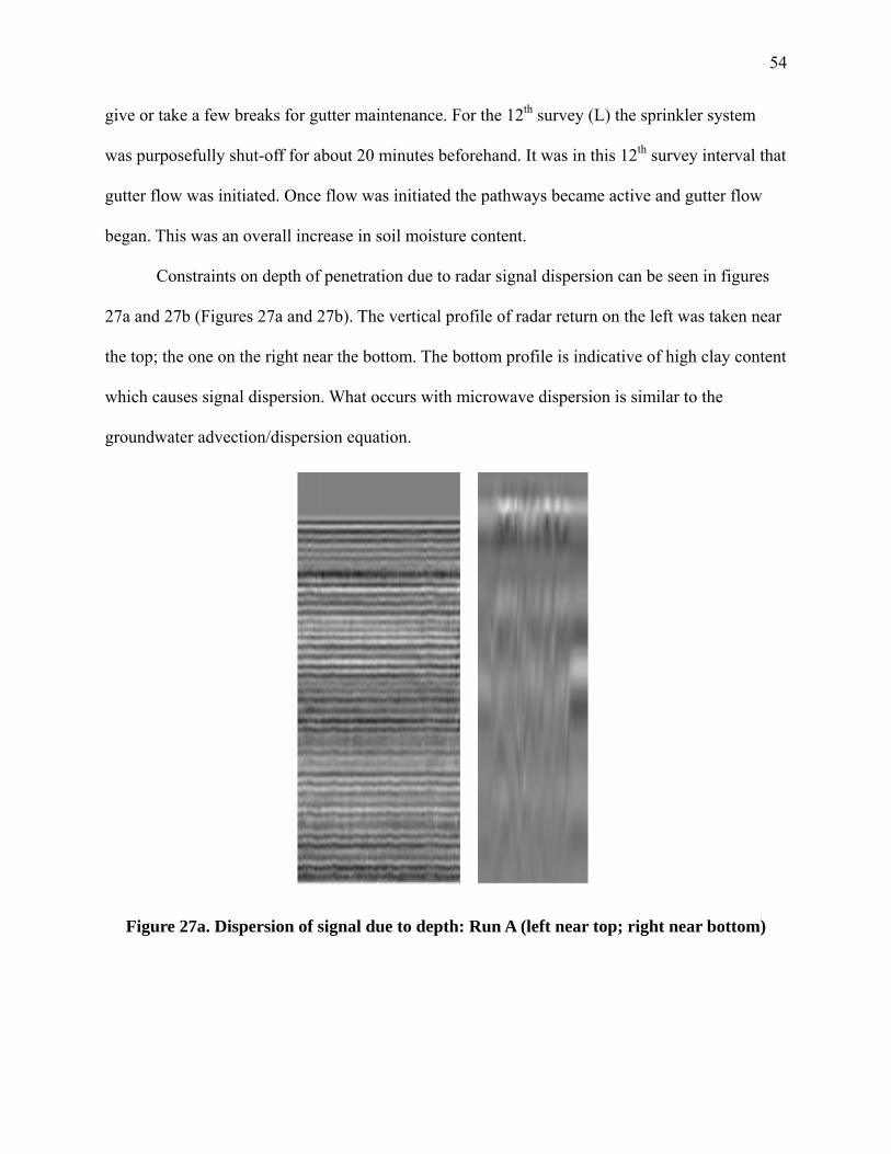
54

give or take a few breaks for gutter maintenance. For the 12th survey (L) the sprinkler system

was purposefully shut-off for about 20 minutes beforehand. It was in this 12th survey interval that

gutter flow was initiated. Once flow was initiated the pathways became active and gutter flow

began. This was an overall increase in soil moisture content.

Constraints on depth of penetration due to radar signal dispersion can be seen in figures

27a and 27b (Figures 27a and 27b). The vertical profile of radar return on the left was taken near

the top; the one on the right near the bottom. The bottom profile is indicative of high clay content

which causes signal dispersion. What occurs with microwave dispersion is similar to the

groundwater advection/dispersion equation.

Figure 27a. Dispersion of signal due to depth: Run A (left near top; right near bottom)

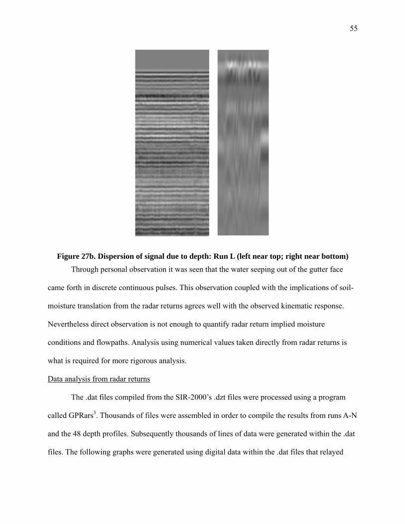
55

Figure 27b. Dispersion of signal due to depth: Run L (left near top; right near bottom) Through personal observation it was seen that the water seeping out of the gutter face

came forth in discrete continuous pulses. This observation coupled with the implications of soil-

moisture translation from the radar returns agrees well with the observed kinematic response.

Nevertheless direct observation is not enough to quantify radar return implied moisture

conditions and flowpaths. Analysis using numerical values taken directly from radar returns is

what is required for more rigorous analysis.

Data analysis from radar returns

The .dat files compiled from the SIR-2000’s .dzt files were processed using a program

called GPRars3. Thousands of files were assembled in order to compile the results from runs A-N

and the 48 depth profiles. Subsequently thousands of lines of data were generated within the .dat

files. The following graphs were generated using digital data within the .dat files that relayed

56

frequency of return (analogous to count per unit area, not radar frequency) and the log-intensity

of radar return signal (Figures 28a-28d).

Figures 28a-28d shows radar return data from runs in which gutter response did not occur

(A-D) as well as runs in which response took place (J-M). Layers 9 and 19 correspond to 5-6 cm

and 11-12 cm depth respectively. Each series of runs corresponds to one sequence of wetting: A-

D took place over two days and J-M took place in one day of wetting. The data in Figures 28a-

28d is a depth distribution for the entire 280 by 200 cm plot for the corresponding return depths.

As can be seen in Figure 28a, the runs over layer 9 (5-6 cm) varied quite a bit in

frequency and intensity. Run A is of the most interest in this case. Figure 28a and Figure 28c

show run A as having returned a signal of broad intensity, at a lower frequency than those in

Figures 28b and 28c. Run A was the first radar survey, taken when the soil was very dry,

probably approaching field capacity. This pre-wetting condition yielded radar returns that

encountered very little in the way of moisture or connected pathways. The image of Run A in

Figure 28d for Layer 19, 11-12 cm, shows a shift in over peak intensity with a slight increase in

depth. This may be due to higher dielectric values as clay content increases with depth.

Figures 28d and 28d represent radar runs J-M. Both runs L and M are post-response.

Intensity has increased by at least 100 for most values during these later days of the six-day

experiment. Examination of Run K is the key here since that survey took place a few hours

before response; this is the image of pre-response. In the upper right-hand graph the intensity

distribution for Run K is broadened. Post-response Run L shows an increased peak frequency of

return a narrowed upper limit of intensity.

The graphs of Layer 19 (11-12 cm) show decreased frequencies yet more narrow ranges

of intensity. The peak intensity shifts one order of magnitude from Run K to Run L. The

57

narrowing of intensity distribution may indicate an increase in connectivity as the entire profile

wets-up with later runs. The shift downwards in peak intensity and frequency from K to L may

indicate an “emptying-out” of water-logged pores. Layer 19 at a depth of 11-12 cm was the

lower limit of the soil face at the very bottom of the wetting profile of interest which was around

10-12 cm. The Run L curve is of significance because this is the GPR-survey that occurred about

10 minutes after response (Figure 28b). Heightened peak intensities as well as a peak frequency

higher than any other curve both coincides with prior response: this is correlation.

Figure 28a. Intensity and frequency by layer, Layer 9, Runs A-D (5-6 cm)

58

Figure 28b. Intensity and frequency by layer, Layer 9, Runs J-M (5-6 cm)

Figure 28c. Intensity and frequency by layer, Layer 19, Runs A-D (11-12 cm)

59

Figure 28d. Intensity and frequency by layer, Layer 19, Runs J-M (11-12 cm)

Another means to analyze this numerical radar return data using GPRars is through an

intensity distribution using selected radar runs with various curves representing depths within

those runs within a fixed coordinate system (Figures 29a-29b). These three-dimensional plots

show continuous distributions of moisture from the ground surface to the lower horizons

(approximately 28 cm below the surface). The intensity distribution of Run A shows a profile

that is dry at pre-wetting conditions (Figure 29a). Clear shifts upwards in peak intensity of

return and frequency occur in the dry profile. Rather than a great amount of soil moisture this

may be more indicative of increased clay content. The lower layers at about 0 to 11 cm (Layer

11) shifts in peak intensity from Runs A through K. By Run K the entire soil profile was kept to

near saturation with breaks only occurring after nightfall. That being said these breaks may have

significantly evaporated much of the moisture from the soil.

The distribution by depth for Run A illustrates textures within the soil not moisture

content shifts (Figure 29a). Since this run GPR survey was taken before wetting the soil is

60

extremely dry towards the top of the profile with higher frequencies and peak log intensities

occurring in the lower layers at the Bt horizon. Wet soil is shifted in dielectric constant towards

higher values. The higher returns in Figure 29a towards the bottom of the profile indicate

increased clay content which is exactly what happens in a Bt horizon. For this dry soil run the

textural changes down the profile are constrained by both the dielectric of soil particles which is

~20 and the increasing clay content towards the bottom of the profile. These radar returns from

data indicate a smooth transition from the A to the B soil horizons due to textural properties. The

dielectric is thus a proxy for soil horizon gradation. For that matter, once a radar signal reaches

layers with significant amounts of clay signals for details become overwhelmed by returns due to

the clay content.

Figure 29a. Intensity and frequency by depth, Run A

61

Figure 29b. Intensity and frequency by depth, Run K

Figure 29c. Intensity and frequency by depth, Run L

62

Figure 29d. Intensity and frequency by depth, Run M

From Runs K through M certain layers indicate an increase in connectivity. The most

marked increase is in Layer 11 which was 6-7 cm in depth. Its highest frequency of return shows

a distribution of about 650 in the graph of Run L. Run L was a survey conducted immediately

after first response. The shifting values from K to L may again indicate increasing connectivity in

Run K and a “relaxation” period post-response during Run L. just prior to Run L it is assumed

that drainage has occurred and the image is that of residual soil moisture. Run K indicates a pre-

threshold condition of soil moisture as intensity of return seems to indicate a broad-based wetting

profile. Curiously its overall distribution resembles that of the pre-wetting run: a smooth curve

with few discontinuities. The difference is in the upper layers where higher values in both

frequency and intensity are visible. This may be the clearest indication of pathway connectivity

within the system.

In post-response L connectivity is indicated through the narrow peak intensity values but

broad-based intensity signal is lost as it is assumed the pores have mostly emptied out. By Run

M, which took place before a much smaller gutter response than previously, values throughout

63

the profile are increasing again. With increased time for experimentation perhaps a continuous

relationship between return and flow could have been gleaned from the data. Ultimately a

continuous time-dependent analysis may be the key to observing the kinematic threshold within

GPR returns.

64

CHAPTER 7

CONCLUSIONS AND FUTURE WORK

The ability to analyze soil moisture utilizing GPR has been proven time and again.

Determining pathways within soil during runoff has proven to be more difficult. The numerical

GPR data in this study gave strong indication of certain conditions inherent before and

immediately after the threshold for kinematic response was reached. Nevertheless the data and

conclusions we presented were those of inference and correlation, not causality. The structure and

mechanisms behind flow pathways (macropores, etc.) has yet to be adequately resolved because

causality is determinant of discrete and concise analytical relationships. Furthermore unsaturated

flow through shallow hydrological systems needs to be directly observed. Correlation has been

achieved through the use of numerical GPR return data to graph intensity and frequency of return.

This is a measure of success although more work is needed in this field to be able to achieve a

clearer understanding of effective relationships.

Future work could involve the use of radar during the entirety of wetting periods to obtain a

clear, time-sequenced picture of hillslope processes. A series of radar image visible as “motion

pictures” coupled with a continuous data stream would be of great significance. This could be

correlated with the monitoring of constant volumetric flow data. Perhaps a radar unit that has built-

in waterproof features could be engineered for operation in real-time. Adaptations from

instruments used in marine or lacustrine environments may be of use in this regard. Since the radar

survey for this study required time to assemble after wetting images are those of residual moisture

patterns. While these patterns are good indicators of flow within the system when coupled with

other forms of analysis they do not produce signals of flow in real-time. Thus another

65

engineering solution could be the development of a compact system that requires little to no

assembly. Better yet a constant monitoring system could be employed. Technical solutions for the

instrumentation used in GPR groundwater analysis are of paramount importance if truly time-

dependent data is to be obtained. Continuous monitoring would allow for the precise moment of

response to be recorded with utmost accuracy.

A possibility for analysis may be implicit in the visual geometry of the return patterns.

Since kinematic pressure initiates a wave perhaps the moisture content with an area results in a

“waveform” pattern. Perturbations in this geometry may occur due to small heterogeneities in

soil texture as affected by the downward pressure. Perhaps there is a functional relationship

between these geometries and the radar return signals. Zones of high dielectric values appear to

shift with some regularity within both the visual patterns and numerical analyses of the GPR

signals. This appears to mimic a waveform in width, breadth and depth.

Continuous records of radar images, radar data and volumetric return data seems to be the

means in obtaining a robust series of said data. Numerical information of such volume and

precision could therefore lead to more rigorous analysis for causal relationships within the system

as observed through GPR return. The causal relationships between flow patterns and GPR could be

determined. The mathematical analysis of these determinants could therefore result in the

derivation of analytical solutions that show clear relationships between radar signal and the

activation of flow pathways. Once the precise moment of kinematic flow initiation is directly

correlated to a true set of radar signals within a carefully mapped volume the method of

formulation for an analytical solution may be at-hand. Furthermore the formulae or set of equations

thus derived may lead to the further understanding of other, related systems.

66

The accurate visualization of subsurface runoff in the field can greatly aid further research

in all fields of soils and hydrology. In using a wealth of available data for assessment purposes a

series of solutions can be derived that lead to a more complete understanding of preferential flow.

This understanding coupled with the implicit, knowledgeable use of GPR could enable agricultural

interests to safely and efficiently utilize resources in the field. Instrumentation may also be

developed that aids in continuous monitoring of flow pathways. These and other methods might

help to spatially and temporally determine the fate of runoff-driven pesticides, aqueous-phase

chemical constituents or biological agents. Knowledge of the mechanisms behind near-surface

flowpaths and the ability to visualize related processes in real-time may be of great benefit to

industries and realms of academic thought that depend on unsaturated flow processes.

67

REFERENCES

Al-Hagrey, S.A., Schubert-Klempnauer, T., Wachsmuth, D., Michaelsen, J., and Meissner, R.

(1999), Preferential flow: first results of a full-scale flow model, Geophysics Journal

International, 138, 643-654.

Baker, R.S. and Hillel, D. (1990), Laboratory Tests of Fingering During Infiltration into Layered

Soils, Soil Science Society of America Journal, 54, 20-30.

Beasley III, E.B.W. (2011), Investigating the Driving Mechanism of Subsurface Runoff Response

on a Vegetated Hillslope in the Georgia Piedmont, M.S. thesis, University of Georgia,

Department of Geology.

Bernier, P.Y. (1986), Variable Source Areas and Storm-Flow Generation: An Update of the

Concept and a Simulation Effort, Journal of Hydrology, 79, 196-213.

Beven, K. and Germann, P. (1982), Macropores and Water Flow in Soils, Water Resources

Research, 18(5), 1311-1325.

Bouma, J. (1981), Soil Morphology and Preferential Flow along Macropores, Agricultural Water

Management, 3, 235-250.

Bradford, J.H. (2008), Measuring Water Content Heterogeneity Using Multifold GPR with

Reflection Tomography, Vadose Zone Journal, 7(1), 184-193.

Brooks, R.H. and Corey, A.T. (1964), Hydraulic Properties of Porous Media. Hydrology Paper

no. 3, Civil Engineering Dept., Colorado State Univ., Fort Collins, Colorado.

Brooks, R.H. and Corey, A.T. (1966), Properties of Porous Media Affecting Fluid Flow, Journal

of the Irrigation and Drainage Division, American Society of Civil Engineers, 92(IR2),

68

61-88.

Burdine, N.T. (1953), Relative Permeability Calculations from Pore-Size Distribution Data,

Transactions of the American Institute of Mining, Metallurgical and Petroleum

Engineers, 198, 71-77.

Carmianti, A., Kaestner, A., Lehmann, P., and Flühler, H. (2008), Unsaturated water flow across

soil aggregate contacts, Advances in Water Resources, 31, 1221-1232.

Chappell, N.A., and Sherlock, M.D. (2005), Contrasting flow pathways within tropical forest

slopes of Ultisol soils, Earth Surface Processes and Landforms, 30, 735-753.

Corey, A.T., and Brooks, R.H. (1975), Drainage Characteristics of Soils, Soil Science Society of

America Proceedings, 39(2), 251-255.

Davis, B.R., Lundien, J.R., and Williamson, Jr., A.N. (1966), Feasibility Study of the Use of

Radar to Detect Surface and Ground Water, U.S. Army Corps of Engineer Waterways

Experiment Station Technical Report, 3(727), 50 pp.

Davis, D.D., Horton, R., Heitman, J.L., and Ren, T. (2009), Wettability and Hysteresis Effects on

Water Sorption in Relatively Dry Soil, Soil Science Society of America Journal, 73(6),

1947-1951.

Doolittle, J. A. and Collins, M. E. (1995), Use of soil information to determine application of

ground penetrating radar, Journal of Applied Geophysics, 33, 101-108.

Doolittle, J.A., Jenkinson, B., Hopkins, D., Ulmer, M., and Tuttle, W. (2006), Hydropedological

investigations with ground-penetrating radar (GPR): Estimating water-table depths and

local ground-water flow pattern in areas of coarse-textured soils, Geoderma, 131, 317-

329.

Doolittle, J. A., Minzenmayer, F.E., Waltman, S.W., Benham, E.C., Tuttle, J.W., and Peaslee,

69

S.D. (2007), Ground-penetrating radar soil suitability map of the conterminous United

States, Geoderma, 141, 416-421.

Endale, D., Fisher, D., and Steiner, J. (2003), Long-Term Rainfall and Runoff Characteristics of a

Small Southern Piedmont Watershed, First Interagency Conference on Research in the

Watersheds, Conference Proceedings, 497-502.

Endale, D.M., Radcliffe, D.E., Steiner, J.L., and Cabrera, M.L. (2003), Drainage Characteristics

of a Southern Piedmont Soil Following Six Years of Conventionally Tilled or No–Till

Cropping Systems, Transactions of the American Society of Agricultural Engineers,

45(5), 1423-1432.

Farmani, M. B., Kitterød, N.-O., and Keers, H. (2008), Estimation of Unsaturated Flow

Parameters Using GPR Tomography and Groundwater Table Data, Vadose Zone Journal,

7(4), 1193-1206.

Farmani, M. B., Kitterød, N.-O., and Keers, H. (2008), Inverse modeling of unsaturated flow

parameters using dynamic geological structure conditioned by GPR tomography, Water

Resources Research, 44(W08401).

Fetter, C.W. (2001), Applied Hydrogeology, 598 pp., Prentice Hall, Englewood Cliffs, N.J.

Freeland, R.S., and Odhiambo, L.O. (2006), Subsurface Characterization Using Textural

Features Extracted from GPR Data, Transactions of the American Society of Agricultural

Biological Engineers, 50(1), 287-293.

Germann, P.F. and Beven, K. A. (1986), Distribution Function Approach to Water Flow in Soil

Macropores Based on Kinematic Wave Theory, Journal of Hydrology, 83, 173-183.

Germann, P.F. and DiPietro, L. (1996), When is porous-media flow preferential? A

hydromechanical perspective, Geoderma, 74, 1-21.

70

Gish, T.J., Dulaney, W.P., Kung, K.–J.S., Daughtry, C.S.T., Doolittle, J.A. and Miller, P.T. (2002),

Evaluating Use of Ground-Penetrating Radar for Identifying Subsurface Flow Pathways,

Soil Science Society of America Journal, 66, 1620-1629.

Gish, T.J., Walthall, C.L., Daughtry, C.S.T., and Kung, K.–J.S. (2005), Using Soil Moisture and

Spatial Yield Patterns to Identify Subsurface Flow Pathways, Journal of Environmental

Quality, 34, 274-286.

Hewlett, J.D. (1961), Soil Moisture as a Source of Base Flow from Steep Mountain Watersheds,

Southeast Forest Experiment Station, Paper 132, 11 pp.

Hewlett, J.D., and Hibbert, A.R. (1963), Moisture and Energy Conditions within a Sloping Soil

Mass During Drainage, Journal of Geophysical Research, 68(4), 1081-1087.

Hewlett, J.D., and Hibbert, A.R. (1966), Factors Affecting the Response of Small Watersheds to

Precipitation in Humid Areas, International Symposium on Forest Hydrology, Penn

State University August 29 – September 10, 1965, Pergamon Press, Oxford & N.Y.

Hewlett, J.D., and Nutter, W.L. (1970), The Varying Source Area of Streamflow From Upland

Basins, Proceedings of the Symposium on Interdisciplinary Aspects of Watershed

Management, Montana State University August 3-6, 1970, American Society of Civil

Engineers, New York, 65-83.

Hillel, D. and Baker, R.S. (1988), A Descriptive Theory of Fingering during Infiltration into

Layered Soils, Soil Science, 146(1), 51-56.

Huisman, J.A., Snepvangers, J.J.J.C., Bouten, W., and Heuvelink, G.B.M. (2002), Mapping

spatial variation in surface soil water content: comparison of ground-penetrating radar

and time reflectometry, Journal of Hydrology, 269, 194-207.

Jadoon, K.Z., Slob, E., Vanclooster, M., Vereecken, H., and Lambot, S. (2008), Uniqueness and

71

stability analysis of hydrogeophysical inversion for time-lapse ground-penetrating radar

estimates of shallow soil hydraulic properties, Water Resources Research, 44(W09421).

Kaiser, D.R., Reinert, D.J., Reichert, J.M., and Minella, J.P.G. (2010), Dielectric Constant

Obtained from TDR and Volumetric Moisture of Soils in Southern Brazil, Revista

Brasileira de Ciência do Solo, 34, 649-658.

Knight, R. (2001), Ground Penetrating Radar for Environmental Applications, Annual Review of

Earth and Planetary Sciences, 29, 229-255.

Lambot, S., Antoine, M., van den Bosch, I. Slob, E.C., and Vanclooster, M. (2004),

Electromagnetic Inversion of GPR Signals and Subsequent Hydrodynamic Inversion to

Estimate Effective Vadose Zone Hydraulic Properties, Vadose Zone Journal, 3, 1072-

1081.

Lambot, S., Slob, E.C., Vanclooster, M., and Vereecken, H. (2006), Closed loop GPR data

inversion for soil hydraulic and electric property determination, Geophysical Research

Letters, 33, L21405.

Lehman, P., Hinz, C., McGrath, G., Tromp-van Meerveld, H.J., McDonnell, J.J. (2007), Rainfall

threshold for hillslope outflow: an emergent property of flow pathway connectivity,

Hydrology and Earth System Sciences, 11, 1047-1063.

Lin, H. (2010), Linking principles of soil formation and flow regimes, Journal of Hydrology, 393

(1-2), 3-19.

Loken, M. (2007), Use of Ground Penetrating Radar to Evaluate Minnesota Roads, Minnesota

Department of Transportation Research Report, MN/RC-2007-01, 45 pp.

Lunt, I.A., Hubbard, S.S., and Rubin, Y. (2005), Soil moisture content estimation using ground-

penetrating radar reflection data, Journal of Hydrology, 307, 254-269.

72

Luxmoore, R.J., Jardine, P.M., Wilson, G.V., Jones, J.R. and Zelazny, L.W. (1990), Physical and

Chemical Controls of Preferred Path Flow Through a Forested Hillslope, Geoderma, 46,

139-154.

McKinnon, R.J. (2006), A Mechanism for Storm Runoff Generation During Large Rainfall

Events, M.S. thesis, University of Georgia, Department of Geology.

Milly, P.C.D. (1985), A mass-conservative procedure for time-stepping in models of unsaturated

flow, Advances in Water Research, 8, 32-36.

Mualem, Y. (1976), A new model for predicting the hydraulic conductivity of unsaturated porous

media, Water Resources Research, 12, 513-522.

Neiber, J.L. and Sidle, R.C. (2010), How do disconnected macropores in sloping soils facilitate

preferential flow? Hydrological Processes, 24, 1582-1594.

Nimmo, J.R. And Landa, E.R. (2005), The Soils Physics Contributions of Edgar Buckingham,

Soil Science Society of America Journal, 69, 328–342.

Pachepsky, Y., Timlin, D., and Rawls, W. (2003), Generalized Richards’ equation to simulate

water transport in unsaturated soils, Journal of Hydrology, 272, 3-13.

Perkins, H. F., (1987). Characterization Data for Selected Georgia Soils, Georgia Agricultural

Experiment Stations, College of Agriculture, The University of Georgia. Athens. Special

Publication 43, 545 pp.

Pettinelli, E., Vannaroni, G., Di Pasquo, B., Mattei, E., Di Matteo, A., De Santis, A., and Annan,

P.A. (2007), Correlation between near-surface electromagnetic soil parameters and early-

time GPR signals: An experimental study, Geophysics, 72(2), A25-A28.

Pilgrim, D. H., Huff, D. D., and Steele, T. D. (1978), A Field Evaluation of Subsurface and

Surface Runoff, II. Runoff Processes, Journal of Hydrology, 38, 319-341.

73

Radcliffe, D.E., and Simunek, J. (2010), Soil Physics with HYDRUS: Modeling and

Applications, 388 pp., CRC Press, Boca Raton, Florida.

Rasmussen, T.C., Baldwin, Jr., R.H., Dowd, J.F., and Williams, A.G. (2000), Tracer vs. Pressure

Wave Velocities through Unsaturated Saprolite, Soil Science Society of America Journal,

64, 75-85.

Rajkai, K., Kabos, S., and Van Genuchten, M.T. (2004), Estimating the water retention curve

from soil properties: comparison of linear, nonlinear and concomitant variable methods,

Soil & Tillage Research, 79, 145-152.

Richards, L.A. (1931), Capillary Conduction of Liquids through Porous Mediums, Physics, 1,

318-333.

Robinson, D.A, Binley, A., Crook, N., Day-Lewis, F.D., Ferre’, T.P.A., Grauch, V.J.S., Knight,

R., Knoll, M., Lakshmi, V., Miller, R., Nyquist, J., Pellerin, L., Singha, K., and Slater, L.

(2008), Advancing process-based watershed hydrological research using near-surface

geophysics: a vision for, and a review of, electrical and magnetic geophysics methods.

Hydrological Processes, 22, 3604-3635.

Selker, J., Parlange, J.-Y., and Steenhus, T. (1992), Fingered Flow in Two Dimensions, 1.

Measurement of Matric Potential. Water Resources Research. 28:9, 2513-2521.

Selker, J., Parlange, J.-Y., and Steenhus, T. (1992), Fingered Flow in Two Dimensions, 2.

Predicting Finger Moisture Profile. Water Resources Research. 28:9, 2523-2528.

Sharma, P.V. (1997), Environmental and engineering geophysics, 475 pp., Cambridge University

Press, Cambridge, UK.

Smettem, K.R.J. (1987), Characterization of Water Entry into a Soil with a Contrasting Textural

Class: Spatial Variability of Infiltration Parameters and Influence of Macroporosity. Soil

74

Science. 144, 3, 167-174.

Smettem, K.R.J., Chittleborough, D.J., Richards, B.G., and Leaney, F.W. (1991), The Influence

of Macropores on Runoff Generation from a Hillslope Soil with a Contrasting Textural

Class, Journal of Hydrology, 122, 235-252.

Thomas, J.B. (2009), Pressure Wave Generation of Runoff in a Convergent Zone. M.S. thesis,

University of Georgia; Department of Geology.

Tindall, J.A., and Kunkel, J.R. (1999), Unsaturated Zone Hydrology for Scientists and

Engineers. New Jersey: Prentice Hall.

Torres, R. (2002), A threshold condition for soil-water transport, Hydrological Processes, 16,

2703-2706.

Van Genuchten, M.T. (1980), A Closed-Form Equation for Predicting the Hydraulic Conductivity

of Soils, Soil Science Society of America Journal, 44, 892-89.

Vasudeo, A.D., Katpatal, Y.B., and Ingle, R.N. (2009), Uses of Dielectric Constant Reflection

Coefficients for Determination of Groundwater Using Ground-Penetrating Radar, World

Applied Sciences Journal, 6(10), 1321-1325.

Williams, A.G., Dowd, J.F., and Meyles, E.W. (2002), A new interpretation of kinematic

stormflow generation, Hydrological Processes, 16, 2791-2803.

Wŏsten, J.H.M., Bannink, M.H., De Gruijter,. J.J., and Bouma, J. A. (1986), Procedure to

Identify Groups of Hydraulic-Conductivity and Moisture-Retention Curves for Soil

Horizons, Journal of Hydrology, 86, 133-145.

Zheng, C. and Gorelick, S.M. (2003), Analysis of Solute Transport in Flow Fields Influenced by

Preferential Flowpaths at the Decimeter Scale, Groundwater, 41(2), 142-155.

75

APPENDIX A: GROUND-PENETRATING RADAR AND TRACER EXPERIMENT TIMELINE

76

77

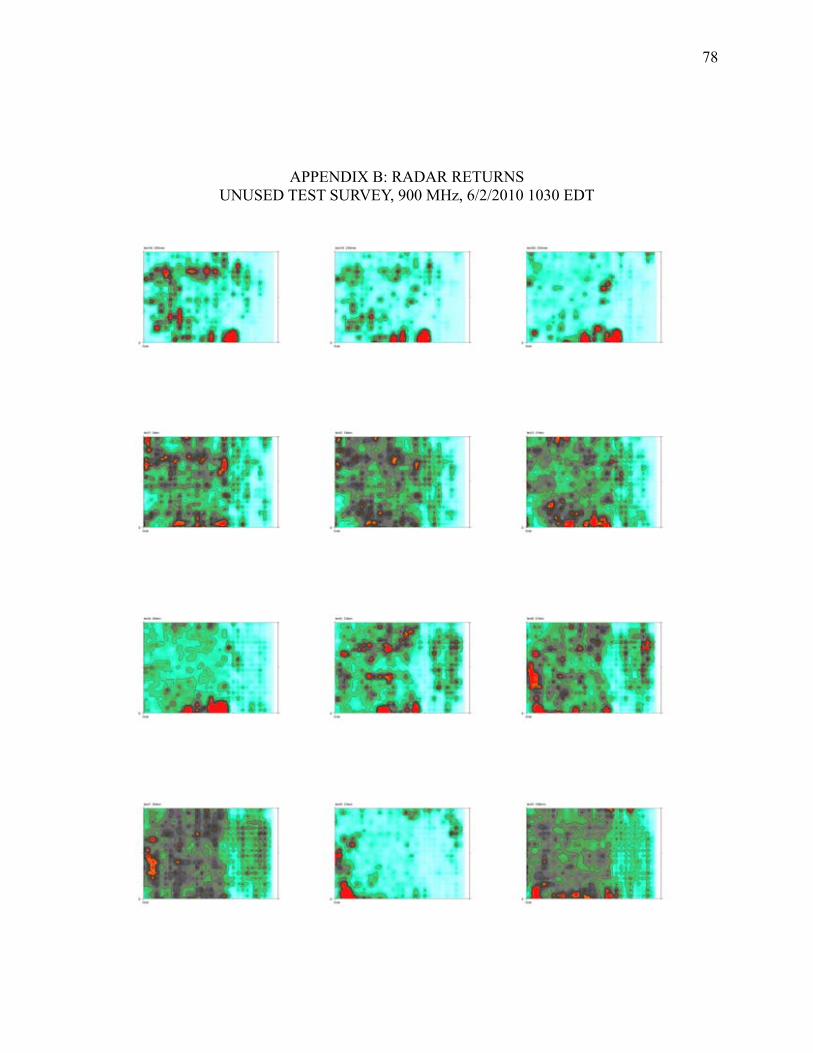
78

APPENDIX B: RADAR RETURNS UNUSED TEST SURVEY, 900 MHz, 6/2/2010 1030 EDT

79

80

1500 MHz, SURVEY A, 6/7/2010, 1338 EDT

81

82

83

84

SURVEY B, 1500 MHz, 6/72011, 1824 EDT

85

86

87

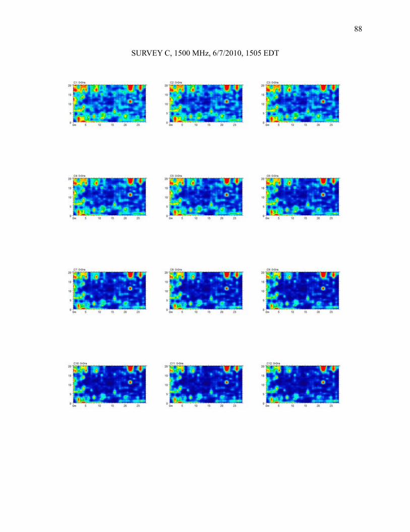
88

SURVEY C, 1500 MHz, 6/7/2010, 1505 EDT

89

90

91

92

SURVEY D, 1500 MHz, 6/8/2010, 1729 EDT

93

94

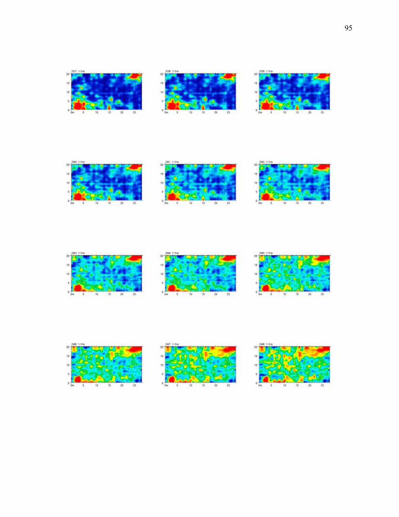
95

96

SURVEY E, 1500 MHz, 6/9/2011, 0910 EDT

97

98

99

100

SURVEY F, 1500 MHz, 6/9/2011, 1120 EDT

101

102

103

104

SURVEY G, 1500 MHz, 6/9/2011, 1447 EDT

105

106

107

SURVEY H, 1500 MHz, 6/10/2011, 1020 EDT

108

109

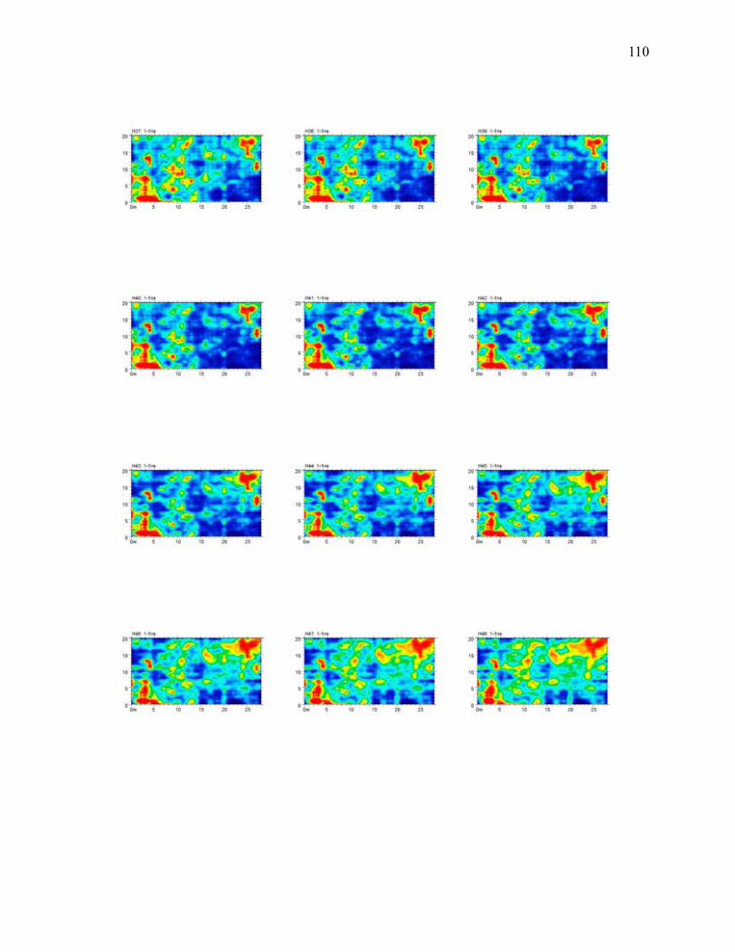
110

111

SURVEY I, 1500 MHz, 6/10/2011, 1409 EDT

112

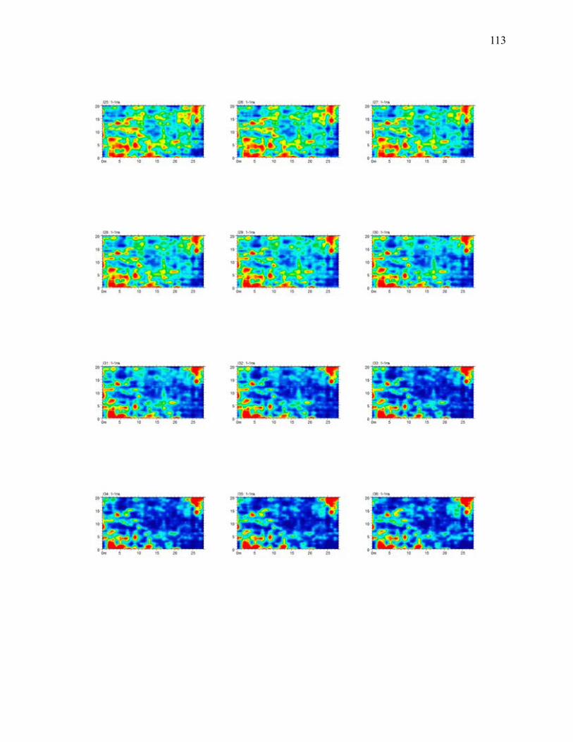
113

114

115

SURVEY J, 1500 MHz, 6/11/2011, 0900 EDT

116

117

118

119

SURVEY K, 1500 MHz, 6/11/2011, 1226 EDT

120

121

122

123

SURVEY L, 1500 MHz, 6/11/2011, 1557 EDT

124

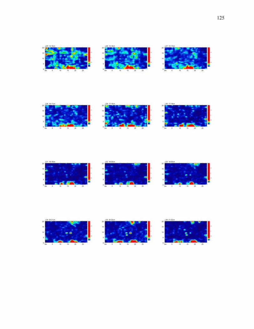
125

126

127

SURVEY M, 1500 MHz, 6/11/2011, 1745 EDT

128

129

130

SURVEY N, 1500 MHz, 06/12/2011, 1348 EDT

131

132

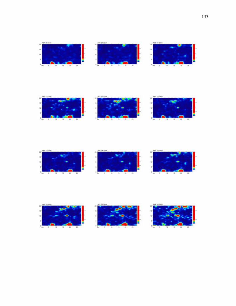
133

134

SURVEY O, 1500 MHz, 06/13/2011, 2102 EDT (UNUSED)

135

136

137

APPENDIX C: TEMPE CELL DATA

138

APPENDIX D: GPR RESOLUTION VS. DIE ECTRIC CONSTANT DURING WETTING: L1500 MHz ANTENNA, AVG. CLAY SOIL

139

140

141