GROSS SUBSTITUTABILITY : AN ALGORITHMIC SURVEY

RENATO PAES LEME∗

Abstract. The concept of gross substitute valuations was introduced by Kelso and Crawford asa sufficient conditions for the existence of Walrasian equilibria in economies with indivisible goods.The proof is algorithmic in nature: gross substitutes is exactly the condition that enables a naturalprice adjustment procedure – known as Walrasian tatonnement – to converge to equilibrium.

The same concept was also introduced independently in other communities with different names:M\-concave functions (Murota and Shioura), Matroidal and Well-Layered maps (Dress and Terhalle)and valuated matroids (Dress and Wenzel). Here we survey various definitions of gross substitutabil-ity and show their equivalence. We focus on algorithmic aspects of the various definitions. Inparticular, we highlight that gross substitutes are the exact class of valuations for which demandoracles can be computed via an ascending greedy algorithm. It also corresponds to a natural discreteanalogue of concave functions: local maximizers correspond to global maximizers.

Finally, we discuss algorithms for the welfare problem (computing an optimal allocation of a setof items when agents have gross substitute valuations) as well as the related problem of computingWalrasian prices. We discuss approximation schemes based on the tatonnement procedure, linearprogramming approaches and purely combinatorial strongly-polynomial time algorithms.

1. Gross substitutes and Walrasian tatonnement. The notion of gross sub-stitutes was introduced by Kelso and Crawford [23] in order to analyze two sidedmatching markets of workers and firms. Originally it was defined as a condition onthe gross product generated by a set of workers for a given firm, hence the name grosssubstitutes. Such condition allowed a natural salary adjustment process to converge toa point where each worker is hired by some firm and no worker is over-demanded. Guland Stacchetti [19] later use the same notion to analyze the existence of price equilib-ria in markets with indivisible goods. For this survey, we adopt the Gul and Stacchettiterminology and talk about buyers/items/prices instead of firms/workers/salaries asin Kelso and Crawford.

Before we proceed, we fix some notation: we denote by [n] = {1, . . . , n} a setof items (goods). A valuation over such items is a function v : 2[n] → R such thatv(∅) = 01. Given a price vector p ∈ Rn and a set S ⊆ [n], we denote p(S) =

∑j∈S pj .

We will define vp(S) = v(S)− p(S) as the value of a subset S under the price vectorp. This corresponds to the utility of an agent with this valuation for acquiring suchset under those prices. Given disjoint sets S, T we define the marginal value of Twith respect to S as v(T |S) = v(T ∪ S) − v(S). We sometimes omit braces in therepresentation of sets when this is clear from the context, for example, by v(i, j|S) wedenote v({i, j}|S).

An economy with indivisible goods is composed by a set [n] of items (goods) and[m] of buyers (agents) where each agent i ∈ [m] has a valuation vi : 2[n] → R. Weuse the notion of the demand correspondence to define an equilibrium of this economy:

Definition 1.1 (demand correspondence). Given a valuation function v : 2[n] →R and a vector of prices p ∈ Rn, we define the demand correspondence as the familyof sets that maximize the utility of an agent under a price vector p :

D(v, p) := {S ⊆ [n]; vp(S) ≥ vp(T ),∀T ⊆ [n]}

∗Google Research NYC, (renatoppl@google.com). Part of this work was done while the authorwas a post-doc at Microsoft Research Silicon Valley.

1Note that we don’t require monotonicity in the definition. When we refer to a valuation forwhich v(S) ≤ v(T ) whenever S ⊆ T , we will refer to it as a monotone valuations or valuationssatisfying free-disposal.

1

Definition 1.2 (Walrasian equilibrium). Given an economy with indivisiblegoods with n goods, m agents and valuations {vi}i satisfying free-disposal2, a Wal-rasian equilibrium corresponds to a vector of prices p ∈ Rn+ and a partition of thegoods in disjoint sets [n] = ∪mi=1Si such that Si ∈ D(vi, p) for all i.

A reader familiar with the duality theorem in linear programming will readilyrecognize that the definition of Walrasian equilibrium closely resembles the com-plementarity conditions where the prices play the role of dual variables. Indeed,this is formalized by the results known as the First and Second Welfare Theorem.The First Welfare Theorem states that if (p, S1, . . . , Sm) is a Walrasian equilib-rium then this partition corresponds to the optimal allocation of goods, i.e., theallocation maximizing

∑i vi(Si). The proof is quite elementary: let S∗1 , . . . , S

∗m be

any partition maximizing the welfare. Then since Si ∈ D(vi, p), it must be thecase that: vi(Si) − p(Si) ≥ vi(S∗i ) − p(S∗i ). Summing for all i and observing that∑i p(Si) = p([n]) =

∑i p(S

∗i ), we conclude that

∑i vi(Si) ≥

∑i vi(S∗i ).

The analogy with linear programming is completed by what is called the SecondWelfare Theorem. It states that if (p, S1, . . . , Sm) is a Walrasian equilibrium andS∗1 , . . . , S

∗m maximizes

∑i vi(S∗i ), then (p, S∗1 , . . . , S

∗m) is also a Walrasian equilib-

rium. The proof is also simple, observe that summing vi(Si)−p(Si) ≥ vi(S∗i )−p(S∗i )for all i we obtain

∑i vi(Si) ≥

∑i vi(S∗i ). But since this is an equality, we should

have an equality for each agent i: vi(Si)−p(Si) = vi(S∗i )−p(S∗i ), hence S∗i ∈ D(vi, p).

A natural question is for which economies there exist Walrasian equilibria. Kelsoand Crawford define a very natural price adjustment procedure and define gross sub-stitutes as the natural sufficient condition for such process to converge. The generalidea behind this procedure goes back to Walras’ tatonnement procedure [45], wheretatonnement means trial-and-error. The idea is that we start with an arbitrary pricevector and compute one set in the demand of each agent. Then, for each item that isdemanded by more then one agent (over-demanded) we increase the price. For eachitem that is demanded by no agent (under-demanded), we decrease the price. Weiterate this until no item is over-demanded or under-demanded.

Let’s describe this procedure precisely. We will make some modifications to theidea above to make the procedure simpler to analyze. Instead of starting from anarbitrary price vector p, we will start with zero prices for all items and only allowprices to increase. Moreover, we will start with all the items allocated to the firstplayer at zero price and we will take turns asking buyers to choose their favorite setof items given prices as follows: the current price pj for items currently allocated tohim and pj + δ for items allocated to other players. Once he takes items from otherplayers, the prices of such items increase by δ.

Notice that the procedure has to stop at some point, since prices cannot increaseindefinitely. If the price of an item is higher then maxi,S v

i(S), for example, no agentwill demand this item and the price will freeze. Let p be the final price and pi bethe price faces by each agent. It should be the case that Si ∈ D(vi, pi), which meansthat for all T ⊆ [n], vi(Si) − pi(Si) ≥ vi(T ) − pi(T ). This can be re-written as:vi(Si)− p(Si) ≥ vi(T )− p(T )− δ|T \ Si|.

2The definition of Walrasian equilibrium can be changed to incorporate valuations not satisfyingfree-disposal. We do so by partitioning the items in m+ 1 disjoint sets S0, S1, . . . , Sm. The items inS0 are not allocated and are required to be priced at zero at in equilibrium.

2

ALGORITHM 1: Walrasian tatonnement procedure

Input: δ > 0, n,m ∈ Z+ and vi for i ∈ [m]Set zero prices for all items: pj = 0, ∀j ∈ [n]Set initial allocation S1 = [n], Si = ∅, ∀i ∈ [m] \ {1}Implicitly define pi ∈ Rn as a function of p s.t. pij = pj if j ∈ Si and pij = pj + δ o.w.while there exists i such that Si /∈ D(vi, pi)

find a demanded set under the pi price vector Xi ∈ D(vi, pi)update prices: for j ∈ Xi \ Si, set pj = pj + δ (vectors pi are implicitly updated)update allocations: Si = Xi and Sj = Sj \Xi for j 6= i

In the limit as δ → 0, we recover a price vector and allocation such that vi(Si)−p(Si) ≥ vi(T ) − p(T ). To make the previous statement precise, let (pt, St1, . . . , S

tm)

be the outcome of the Walrasian tatonnement procedure for δt = 1t for t ∈ Z+. Since

there are finitely many allocations (St1, . . . , Stm), there is one allocation that happens

infinitely often. Let S1, . . . , Sm be such allocation and let t1 < t2 < . . . be theinfinite subsequence corresponding to this allocation. Since pt is bounded, passing toa subsequence if necessary, we can assume that pt → p. So taking t → ∞ for thissubsequence, we get vi(Si)− p(Si) ≥ vi(T )− p(T ) for all i and T ⊆ [n].

The argument above gives us an existential proof of a price vector p and an allo-cation Si such that each agent is getting his optimal bundle under the current prices.This is not yet a Walrasian equilibrium, since Definition 1.2 requires the allocationto be a partition of the set of items, i.e., ∪iSi = [n]. The definition of gross substi-tutability is exactly what is needed to ensure that we can run the procedure above insuch a way that all the items are allocated in the end. Since we started the Walrasiantatonnement procedure with a partition of the items, if we can always find a demandedset Xi ∈ D(vi, pi) containing his currently allocated items, i.e., Si ⊆ Xi, then we canguarantee the invariant that no item is even un-allocated during the execution of thealgorithm. This motivates the following definition:

Definition 1.3 (gross substitutes, Kelso and Crawford [23]). A valuation func-tion satisfies the gross substitutes property if for any price vectors p ∈ Rn andS ∈ D(v, p), if p′ is a price vector with p ≤ p′, then there is a set S′ ∈ D(v, p′)such that S ∩ {j; pj = p′j} ⊆ S′.

In other words: if an agent with a gross substitute valuation demands a set S ofitems under a price vector p and the price of some items subsequently increase, theagent still has a demanded set that contains the items in S whose price didn’t increase.

Theorem 1.4 (Kelso and Crawford [23]). If valuations v1, . . . , vm satisfy thegross substitutes property, then a Walrasian equilibrium always exists.

In some sense, gross substitutability is also necessary for the existence of Wal-rasian equilibria. Gul and Stacchetti [19] show the following: let C be a class ofvaluation functions that contains all unit demand valuations, i.e., all valuations of thetype v(S) = maxj∈S v({j}). Then if C is such that for all v1, . . . , vm ∈ C there is aWalrasian equilibrium, then all valuations in C are gross substitutes.

2. Examples, Non-Examples and Submodularity. It is instructive to havein mind a couple of examples and non-examples of gross substitute functions, to guide

3

our intuition in the following sections. Three simple classes of valuations that can bereadily recognized as gross substitutes from Definition 1.3 are:

1. additive valuations, i.e., valuations for which v(S) =∑i∈S v({i})

2. unit-demand valuations, i.e., valuations for which v(S) = maxi∈S v({i})3. symmetric concave valuations, i.e., valuations of the form v(S) = f(|S|) for

some monotone concave function f : R+ → R+.

A less obvious example is the class of valuations known as assignment valuationsintroduced by Shapley [42], also called OXS valuations by Lehmann, Lehmann andNisan [29]. An assignment valuation with n items can be represented as an n × kmatrix V with non-negative entries, where each row corresponds to an item and eachcolumn to a position. Entry Vi,j corresponds to the value of item i in position j.Each item can be assigned to a single position and each position can be assigned onlyone item. The value of a subset S of items is the value of the optimal assignmentof items in S to positions. Items and positions are allowed to be left unassigned.Mathematically:

v(S) = max{∑i,j Vij · xij s.t.

∑k xkj ≤ 1,

∑k xik ≤ 1 and xij ∈ {0, 1},∀i, j}

We postpone until Section 8 a proof that all assignment valuations are gross substi-tutes, but we remark that unit-demand functions are the special case where there isonly one position, additive functions correspond to the case where the matrix is ann× n diagonal matrix and the symmetric concave valuations to the case in which allthe rows of the matrix are equal.

Hatfield and Milgrom [1] define a generalization of assignment valuations, whichthey call endowed assignment valuations. The show that this class also satisfied thegross substitutes property and that it captures most practical applications of grosssubstitutes valuations in matching markets. A valuation v on n items is said to be anendowed assignment valuation if there is an assignment valuation w on a larger set ofitems such that v(S) = w(S|T ).

Another important example of gross substitutes is the class of matroid rank func-tions. This survey won’t formally require any knowledge of matroid theory, basicfamiliarity with matroids will be useful to guide the reader’s intuition later on. Thetopic is too extensive to survey here, but we point to Lawler [28], Oxley [38] or Schri-jver [41] for a comprehensive discussion.

We remark that even though matroid rank functions are gross substitute val-uations, sums of matroid rank functions might not be. For example, given threeitems {a, b, c} define for each i ∈ {a, b, c}, the function ri : 2{a,b,c} → R such that:ri(∅) = 0, ri(S) = 1 for |S| = 1, ri({a, b, c} \ i) = 1, and ri(S) = 2 for all remainingsubsets S. Notice that for each i, ri is a matroid rank function and hence satisfythe gross substitutability. However, the valuation v = ra + 2 · rb + 3 · rc does notsatisfy gross substitutability. In order to see that, observe that for the price vectorp = [4, 5, 4], D(v; p) = {{a}, {c}, {a, c}, {b, c}}. If the price of item c increases to ∞,i.e., p′ = [4, 5,∞], then demand set becomes D(v; p′) = {{a}}. So the increase in priceof item c makes item b no longer belong to any demanded set, violating Definition 1.3.

Gul and Stachetti [19] observe that gross substitutes are a subclass of submodularfunctions:

4

Definition 2.1 (submodularity). A valuation function is said to be submodularif for all subsets S, T ⊆ [n], v(S ∩ T ) + v(S ∪ T ) ≤ v(S) + v(T ). Equivalently, forevery S ⊆ [n] and i, j /∈ S, v(i, j|S) ≤ v(i|S) + v(j|S).

Theorem 2.2 (Gul and Stacchetti [19]). Every gross substitute valuation func-tion is submodular.

Proof. Let v be a gross substitute valuation functions. Given S ⊆ [n] and i, j /∈ S,consider the price vector3 such that pt =∞ for t /∈ S∪{i, j}, pt = −∞ for t ∈ S∪{j}and pi = v(i|S ∪ {j}). Clearly S ∪ {i, j} ∈ D(v, p). Now, if one defines p′ such thatp′j = ∞ and p′t = pt for all other t, then by gross substitutability, S ∪ {i} must be ademanded set. Therefore: v(i|S) ≥ v(i|S ∪ {j}).

Since the example v = ra+2 ·rb+3 ·rc earlier in this section is the sum of matroidrank functions, and hence submodular, it is clear that gross substitutes is a strictsubclass of submodular functions. Another good source of examples of submodularbut not gross substitute functions comes from the class of budget additive functions.We say that a valuation function is budget additive if it is of the form: v(S) =min{B,

∑i∈S wi} for non-negative real numbers B,w1, . . . , wn. The following example

due to Lehmann, Lehmann and Nisan [29] shows function that is budget additive butnot gross substitutes: consider three items {a, b, c} with weights wa = wb = 1 andwc = 2 and budget B = 2. In order to see that the associated budget additive functionis not gross substitutes, notice that for the prices p = [ 12 ,

12 , 1], D(v, p) = {{a, b}, {c}},

but if the price of a increases and the price vector becomes p′ = [1, 12 , 1], then thedemand correspondence becomes D(v, p′) = {{c}}, i.e., the increase in the price of amakes item b be no longer demanded.

3. Gross substitutes, greedy demand oracles and local search. An im-portant property of gross substitute valuations is that it is the exact class of functionsfor which demand oracles can be computed via a greedy or local search algorithms. Inthis section we make this statement precise by defining matroidal maps and discreteconcave valuations. The first part of the survey will be devoted to show that thosethree concepts are equivalent.

An algorithmic primitive needed to implement the Walrasian tatonnement pro-cedure is the computation of a set in the demand correspondence X ∈ D(v, p). Thisis usually referred as the demand oracle problem. A simple heuristic to compute de-mand oracles is the greedy algorithm: start with the empty set X and keep addingthe element j /∈ X that gives the maximum improvement to vp(X). In other words:

Definition 3.1 (matroidal map). A valuation function is a matroidal map iffor all price vectors p ∈ Rn, the greedy algorithm implements a demand oracle, i.e.,G(v, p) ∈ D(v, p), where G(v, p) is the output of Algorithm 2.

Theorem 3.2. A valuation function satisfies the gross substitute property if andonly if it is a matroidal map.

Before we proceed with the task of proving the previous theorem, we also mention

3allowing prices to take values∞ and −∞ simplifies the arguments. To be more precise, one canview such prices as M or −M for M = 1 + maxS v(S).

5

ALGORITHM 2: Greedy demand oracle

Input: p ∈ Rn+, v : 2[n] → R+

Initialize X = ∅repeat

find j∗ ∈ [n] \X maximizing ∆j = v(j|X)− pjif ∆j∗ > 0, X = X ∪ {j∗}if X = [n] or ∆j∗ ≤ 0, return X

another algorithmic definition of gross substitutability based on local search. Considerthe following heuristic to compute demand oracles: start at an arbitrary set X andtry to find a set improving vp in the neighborhood N of X, where the neighborhoodis composed by all sets that can be obtained from X by adding one element, removingone element or exchanging an element in the set by one element outside the set.

ALGORITHM 3: Local search demand oracle

Input: p ∈ Rn+, v : 2[n] → R+, X0 ⊆ [n]

Initialize X = X0

repeatLet N = {X ∪ {i}; i /∈ X} ∪ {X \ {i}; i ∈ X} ∪ {X ∪ {i} \ {i′}; i /∈ X, i′ ∈ X}If maxY ∈N vp(Y ) ≤ vp(X), return XElse choose some Y ∈ N with vp(Y ) > vp(X) and let X = Y .

Gul and Stacchetti [19] show that yet another way of defining gross substitutesis as the class of valuation functions for which local search is exact, i.e., it doesn’t getstuck on local minima:

Definition 3.3 (discrete concave valuation). A valuation function is discreteconcave if for all price vectors p ∈ Rn, the local search algorithm implements a demandoracle, i.e., L(v, p,X0) ∈ D(v, p), where L(v, p,X0) is the output of Algorithm 3.

Equivalently, a valuation function is discrete concave if and only if for all pricevectors p ∈ Rn, S ∈ D(v, p) iff vp(S) ≥ vp(S ∪ i), vp(S) ≥ vp(S \ j) and vp(S) ≥vp(S ∪ i \ j), for all i /∈ S and j ∈ S.

Theorem 3.4 (Gul and Stacchetti [19]). A valuation function satisfies the grosssubstitute property if and only if it is discrete concave.

4. A price independent local characterization. We make a brief detour andlook at a different, yet very related question about gross substitutes. In the previoussection we gave two alternative algorithmic characterizations of gross substitutes. Allcharacterizations given so far involve prices, i.e., they are of the form: a valuation vsatisfied the gross substitutes property if for all price vectors p, the pair (v, p) has somegiven property. The question of giving an explicit characterization of gross substituteswas resolved simultaneously by Fujishige and Yang [16] and Reijnierse, Gellekom andPotters [39]. The first paper provides a powerful connection to the theory of DiscreteConvex Analysis, which we discuss in more detail in Section 7. We focus first on thedefinition given by Reijnierse et al [39].

6

Theorem 4.1 (Reijnierse, Gellekom and Potters [39]). A valuation function hasthe gross substitutes property iff it is submodular and for all sets S ⊆ [n] and alldistinct i, j, k /∈ S, the following holds:

v(i, j|S) + v(k|S) ≤ max [ v(i|S) + v(j, k|S), v(j|S) + v(i, k|S) ] (RGP)

Proof sketch. The high level picture of their proof is quite simple and illuminating.Here we provide a brief sketch of it. First, they show that a function doesn’t havethe gross substitutes property iff it is possible to find the following certificate: a pricevector p ∈ Rn such that

either (i) D(v, p) = {S, S ∪ {i, j}} or (ii) D(v, p) = {S ∪ {k}, S ∪ {i, j}}.

Notice that the existence of such certificate clearly shows the violation of gross sub-stitutability: the increase in the price of j would make the demand set become {S}in case (i) and {S ∪ {k}} in case (ii). Therefore, item i would no longer be in thedemand set. Proving the other direction requires more work, but its essence is tosearch for a minimal violation of gross substitutability by starting with an arbitraryone and changing the price vector so to shrink the demand set until it is minimal.

The second step is to transform the existence of certificates as above in simpleconditions on v. This is based on two observations: There exists a certificate of type(i) iff the v is not submodular. There exists a certificate of type (ii) iff there is aviolation of condition (RGP).

First, assume that we have a certificate of type (i). So, there are prices such that0 = v(i, j|S)− pi − pj > max[v(i|S)− pi, v(j|S)− pj ]. Summing the inequalities 0 >v(i|S)−pi and v(i, j|S)−pi−pj > v(j|S)−pj we get: v(i, j|S) > v(i|S)−v(j|S) whichis a violation of submodularity. Conversely, if you have a violation of submodularityfor i, j, S, take pt = −∞ for t ∈ S, pt = ∞ for t /∈ S ∪ {i, j} and pi = v(i|S) + ε andpj = v(j|S) + ε for some tiny ε and this gives us a certificate of type (i).

Assume now that we have a certificate of type (ii). So, there are prices suchthat v(k|S) − pk = v(i, j|S) − pi − pj > max[v(i|S) − pi, v(j|S) − pj , v(i, k|S) − pi −pk, v(j, k|S)− pj − pk]. Summing the inequalities such that the prices cancel, we get:v(i, j|S) + v(k|S) > max[v(i|S) + v(j, k|S), v(j|S) + v(i, k|S)]. Conversely, if you havea violation of the condition (RGP) for i, j, k, S, let φ > 0 be the value of the violation,i.e., φ = v(i, j|S) + v(k|S)−max{v(i|S) + v(j, k|S), v(j|S) + v(i, k|S)}. Now, considerprices pt = −∞ for t ∈ S, pt = ∞ for t /∈ S ∪ {i, j, k} and pi = v(i|S ∪ {j}) − 1

2φ,pj = v(j|S ∪{i})− 1

2φ and pk = v(k|S) + v(i, j|S)− v(i|S)− v(j|S)−φ. It is straight-forward to check that such prices give us a certificate of type (ii).

Now we explain what we mean by a local characterization. Given a valuationfunction v and two sets S,R ⊆ [n] we can define a restriction vR|S : 2R → R byvR|S(T ) = v(T |S). We say that this is a k-restriction if |R| = k. Observe that usualproperties as monotonicity and submodularity are properties of the restrictions, i.e.,a function is monotone iff each 1-restriction is monotone. A function is submodulariff each 2-restriction is submodular. A corollary of Theorem 4.1 is that:

Corollary 4.2. A valuation function satisfies the gross substitutes property iffevery 3-restriction satisfied the gross substitutes property.

7

An equivalent characterization of the one in Theorem 4.1 was also observed inLehmann, Lehmann and Nisan [29] and Bing, Lehmann and Milgrom [7]. The lattercharacterization defines for each valuation v and subset S ⊆ [n] a measure of how twogoods i and j are substitutes to each other. Given i, j /∈ S, let:

αS(i, j) = v(i|S) + v(j|S)− v(i, j|S)

and observe that (RGP) is equivalent to αS(i, j) ≥ min[αS(i, k), αS(k, j)]. This inparticular says that dS(i, j) = αS(i, j)−1 is a metric satisfying the following strongerversion of the triangle inequality: dS(i, j) ≤ max[dS(i, k), dS(k, j)]. Such metrics arecalled ultra-metrics and have the interesting properties that all triangles are isosceles.This translates back to αS as saying that given {i, j, k}, then up to renaming we have:

αS(i, k) = αS(k, j) ≤ αS(i, j) (Iso)

We observe one interesting non-trivial and useful consequence of the isosceles tri-angle property, which will be useful later:

Lemma 4.3. Given a gross substitute valuation v : 2[n] → R, S ⊆ [n] andi1, i2, j1, j2 /∈ S, then:

v(i1, i2|S) + v(j1, j2|S) ≤ max[v(i1, j2|S) + v(j1, i2|S), v(i1, j1|S) + v(i2, j2|S)]

Proof. Let P = {i1, i2, j1, j2} and M = min{t1,t2}∈P αS(t1, t2). Define the lengthof the edge between (t1, t2) as αS(t1, t2). By property (Iso), every triangle is isosceleswith the smaller edge appearing at least twice. So, if we look the graph of the edgesof minimal length between P , then either one of two things happen: (i) there is acycle, i.e., there are αS(x1, x2) = αS(x2, x3) = αS(x3, x4) = αS(x4, x1) = M where{x1, x2, x3, x4} = {i1, i2, j1, j2} or (ii) there is a star, i.e., αS(x1, x2) = αS(x2, x3) =αS(x2, x4) = M . In order to see that, let x1, x2 be nodes in P such that αS(x1, x2) =M . Let x3 be some other node, so the triangle x1, x2, x3 must have two sides of lengthM . Up to renaming, αS(x1, x2) = αS(x2, x3) = M . If αS(x2, x4) = M we are in case(ii). If αS(x2, x4) > M then by property (Iso) applied on the triangles x1, x2, x4 andx2, x3, x4, we must have αS(x1, x4) = αS(x3, x4) = M , in which case we are in case(i).

Now, proving the statement of the lemma in each of the two cases is simple: ifwe are in case (i), then we can assume (swapping the names of i1, i2 if necessary)that αS(i1, j1) = αS(i2, j2) = M , so: αS(i1, j1) + αS(i2, j2) = 2M ≤ αS(i1, i2) +αS(j1, j2), which is equivalent to the statement in the lemma. In case (ii), say i1 isthe center of the star, i.e., αS(i1, x) = M for all x ∈ {i2, j1, j2}. Now: αS(j1, j2) ≥min[αS(i2, j1), αS(i2, j2)]. Swapping the names of j1 and j2 if necessary, we canassume that: αS(j1, j2) ≥ αS(i2, j1). That together with αS(i1, i2) = M = αS(i1, j2),we get again αS(i1, j1) +αS(i2, j2) ≤ αS(i1, i2) +αS(j1, j2) which is equivalent to thestatement in the lemma.

5. Well Layered and Matroidal Maps. The final step towards proving theequivalence of definitions 3.1 and 1.3 is the concept of well layered maps introducedby Dress and Terhalle [11] – in which the authors characterize the set functionsv : 2[n] → R for which greedy algorithms are optimal.

8

Definition 5.1 (well-layered map). A function v : 2[n] → R is called well-layered iff for each p ∈ Rn the sets S0, S1, S2, . . . obtained by the greedy algorithm(i.e., S0 = ∅ and Si = Si−1 ∪ {xi} where xi ∈ argmaxx∈[n]\Si−1

vp(x|Si−1)) are suchthat vp(Si) = max{vp(S); |S| = i}.

Theorem 5.2 (Dress and Terhalle [11]). A map v : 2[n] → R is well-layered ifffor any triple of disjoint sets S, {i}, T with |T | ≥ 2,

v(i|S) + v(T |S) ≤ maxj∈T

v(j|S) + v(T ∪ i \ j|S) (WL)

Before we proceed to the proof of Theorem 5.2 it is useful to notice its relationwith the condition of Reijnierse et al:

Lemma 5.3. Conditions (RGP) and (WL) are equivalent.Proof. One readily recognizes condition (RGP) to be a special case of (WL) with

|T | = 2. For the other direction, we show by induction on |T | that (RGP) implies(WL). For |T | = 2, this is trivial. Now, suppose we proved it for |T | = t − 1. GivenS, {i}, T with |T | = t, choose k ∈ T minimizing αS(i, k). Then by the inductionhypothesis applied to S ∪ k, {i}, T \ k, we have that there is j ∈ T \ k such that:

v(i|S ∪ k) + v(T \ k|S ∪ k) ≤ v(j|S ∪ k) + v(T ∪ i \ j, k|S ∪ k)

which can be re-written as:

v(i, k|S) + v(T |S) ≤ v(j, k|S) + v(T ∪ i \ j|S)

now notice that by the choice of k, it must be the case that for all j, αS(i, k) ≤ αS(k, j),since the smaller αS-value in the triangle i, j, k appears twice and αS(i, k) ≤ αS(i, j).Now, this means that v(i|S)− v(i, k|S) ≤ v(k|S)− v(j, k|S). Summing with the pre-vious inequality gives us condition (WL) for |T | = t.

Proof of Theorem 5.2. First, assume that the condition (WL) holds and let’sprove that St ∈ argmaxS;|S|=tvp(S) by induction on t. The case t = 1 is trivial.Assume we proved for t− 1 and assume there is S′ with |S′| = t and vp(S

′) > vp(St).Choose such set maximizing k such that {x1, . . . , xk} ⊆ S′. Since |S′| = |St| = t,clearly k < t. Now, applying (WL) for {x1, . . . , xk}, xk+1, T

′ = S′ \ {x1, . . . , xk} weget that there is j ∈ T ′ such that:

v(xk+1|x1, . . . , xk) + v(T ′|x1, . . . , xk) ≤ v(j|x1, . . . , xk) + v(T ′ ∪ xk+1 \ j|x1, . . . , xk)

and since v(xk+1|x1, . . . , xk) ≥ v(j|x1, . . . , xk) by the greedy rule, we have thatv(S′) ≤ v(S′ ∪ xk+1 \ j) contradicting the minimality of k.

For the other direction, assume that (WL) is violated. Since (WL) is equivalentto (RGP), (WL) must be violated by some |T | = {j, k}. So assume S, i, {j, k} forwhich (WL) is not valid. Now, define prices such that pt = −∞ for t ∈ S, pt =∞ fort /∈ S ∪ {i, j, k}, pi = v(i|S)− ε, pj = v(j|S) and pk = v(k|S). The greedy algorithmwill first pick all the elements in S, then i. Now, observe that for t = |S| + 2 theoptimal set is either S∪{i, j}, or S∪{j, k} or S∪{i, k}. The fact that (WL) is violatedimplies that v(i|S) + v(j, k|S) > v(j|S) + v(i, k|S). Substituting v(i|S) and v(j|S) by

9

the prices, we get that (for sufficiently small ε) v(j, k|S)−pj−pk > v(i, k|S)−pi−pk,i.e., S ∪ {j, k} is strictly preferable then S ∪ {i, k}. The exact same argument worksswapping j and k, so the only set of size |S|+2 maximizing vp is S∪{j, k}. Thereforev can’t be a well-layered map, since the greedy algorithm picked i in step |S|+1. Thisfinishes the proof of Theorem 5.2.

The concept of well layered maps guarantees that the greedy algorithm will findthe optimal set of each cardinality. In order to guarantee that the greedy algorithmas described in Section 3 will find the optimal, we need to guarantee that once a layerdoesn’t improve over the previous, we can stop. Dress and Terhalle [10] observe thatin order for this to happen, it is necessary and sufficient that the valuation is bothwell-layered and submodular. They call such functions matroidal maps.

Theorem 5.4 (Dress and Terhalle [10]). A valuation function satisfied Defini-tion 3.1 iff it is well-layered and submodular.

Proof. Submodularity guarantees that the sets St will be such that vp(St+1) −vp(St) ≤ vp(St ∪xt+1 \xt)− vp(St−1) ≤ vp(St)− vp(St−1). So: vp(St) ≥ 1

2 [vp(St−1) +vp(St+1)]. This guarantees that t 7→ vp(St) is concave. For the converse, if a functionis not submodular, then there exist i, j, S such that v(i, j|S) > v(i|S) + v(j|S). Soone can set prices pt = −∞ for t ∈ S, pt = ∞ for t /∈ S ∪ {i, j}, pi = v(i|S) + ε andpj = v(j|S) + ε for some small ε. For such prices the greedy algorithm will terminateon S, while the optimum is S ∪ {i, j}.

Theorem 5.4 establishes our main claim that Definitions 3.1 and 1.3 are equiva-lent. In particular, for any gross substitute valuation function, a set S ∈ D(v; p) canbe found using the greedy algorithm (Algorithm 2). The following remark states thatthe greedy algorithms finds not only one, but all demanded sets. This fact is somehowimplicit in the proof of Theorem 5.4 but we state and prove it again for completeness:

Remark 5.5. Given a gross substitute valuation function v, a price vector pand a demanded set S ∈ D(v; p), then there is a tie breaking rule4 for the greedyalgorithm that produces the set S. Formally, if x1, x2, . . . , xk is an ordering of ele-ments in S such that xi ∈ argmaxy∈S\{x1,...,xi−1}v(y|x1, . . . , xi−1), then xi is also inargmaxy∈[n]\{x1,...,xi−1}v(y|x1, . . . , xi−1).

Proof. This fact follows directly from the (WL) condition. Assume that thereis i such that for some vp(y|x1, . . . , xi−1) > vp(xi|x1, . . . , xi−1). Since x1, . . . , xkare in greedy order, it must be that y /∈ S. By applying (WL) with sets Xi−1 ={x1, . . . , xi−1}, {y}, {xi, . . . , xk}, we get that there is xt for t ≥ i such that:

vp(y|Xi−1) + vp(xi, . . . , xk|Xi−1) ≤ vp(xt|Xi−1) + vp({y, xi, . . . , xk} \ xt|Xi−1)

Since vp(y|Xi−1) > vp(xi|Xi−1), we get vp(S) < vp(S ∪ y \xt), which contradicts thatS ∈ D(v; p).

We would like to finish by pointing out that many combinatorial structures suchas matroids, polymatroids, valuated matroids [12], among others, can be defined as

4formally a tie breaking rule is a function b that associates for each pair of disjoint sets S, T anelement from T . The greedy algorithm with tie-breaking rule b, whenever choosing an element inT = argmaxi/∈Sv(i|S), it adds b(S, T ) ∈ T .

10

the class of objects for which a certain problem admits a greedy solution. For a moreextensive exposition on such combinatorial structures we refer to the classical textof Korte, Lovasz and Schrader on greedoids [26]. Similar arguments can be used toargue about local search:

Theorem 5.6. A valuation function satisfied Definition 3.3 iff it is well-layeredand submodular.

Proof. First we argue that if a valuation v is well-layered and submodular,then local search can’t get stuck in a local maximum for any price p. Let S∗ ∈argmaxS⊆[n]vp(S) and S ⊆ [n] be such that vp(S) < vp(S

∗). Then we want to arguethat there is S′ ∈ N where N is the neighborhood of S as in the local search proce-dure in Section 3. First observe that if v is well-layered and submodular, then vp hasalso those two properties.

We consider three cases:

Case (i) S ⊆ S∗. Notice that 0 < vp(S∗ \ S|S) ≤

∑i∈S∗\S vp(i|S), where the last

inequality follows from submodularity. Therefore, there is some i for which vp(i|S) >0, then we can take S′ = S ∪ {i}.

Case (ii) S∗ ⊆ S. Let S \ S∗ = {i1, . . . , ik} For this case, 0 > vp(S \ S∗|S∗) =∑kj=1 vp(ij |S ∪ {i1, . . . , ij−1}) ≥

∑kj=1 vp(ij |S \ ij). So there must be i ∈ S \ S∗ such

that vp(i|S \ i) < 0, then we can take S′ = S \ i.Case (iii) if neither S ⊆ S∗ nor S∗ ⊆ S, let i be the element in (S \S∗)∪ (S∗ \S)

maximizing vp(i|S ∩ S∗). Now, we consider two possibilities: (iii-a) If i ∈ S∗, we usecondition (WL) with S ∩ S∗, i, S \ S∗. This gives us j ∈ S \ S∗ such that:

vp(i|S ∩ S∗) + vp(S \ S∗|S ∩ S∗) ≤ vp(j|S ∩ S∗) + vp((S \ S∗) ∪ i \ j|S ∩ S∗)

By the choice of i, we know that vp(j|S ∩ S∗) ≤ vp(i|S ∩ S∗). If this inequalityholds strictly, then, vp(S \ S∗|S ∩ S∗) < vp((S \ S∗) ∪ i \ j|S ∩ S∗) and thereforevp(S) ≤ vp(S ∪ i \ j). If on the other hand vp(j|S ∩ S∗) = vp(i|S ∩ S∗) then wecan swap i and j and consider the sub-case where i ∈ S. (iii-b) If i ∈ S, we usecondition (WL) with S ∩ S∗, i, S∗ \ S. Doing as above, we find j ∈ S∗ \ S such thatvp(S

∗) ≤ vp(S∗ ∪ i \ j), which holds with equality since S∗ is optimal. This way

we obtain an optimal set closer to S. Then we can repeat the above procedure withS∗ ∪ i \ j instead of S∗ a finite number of times until we reach some set S′ ∈ N or wereach one of the previous cases.

For the converse direction, we want to show that if a valuation is not well-layeredor not submodular, local search can get stuck in suboptimal local minima. For this,we can use the same examples used to show that in such case the greedy algorithmcan be suboptimal.

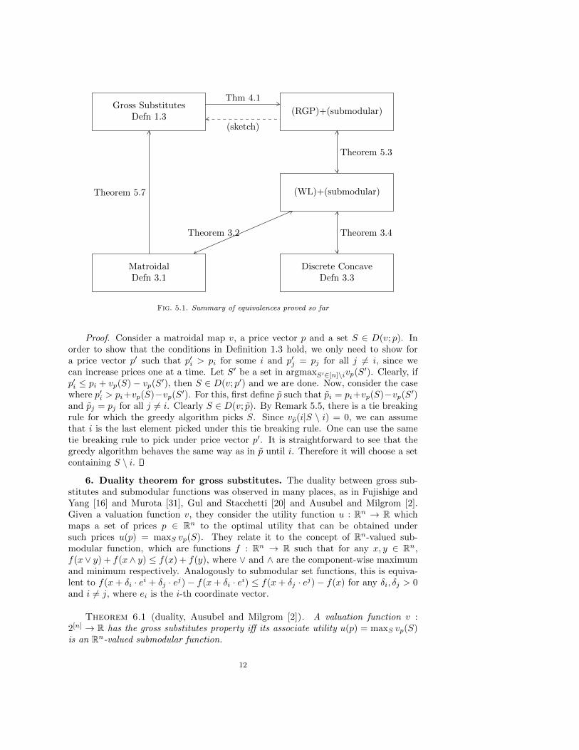
We end this section with Figure 5.1 summarizing the equivalences proved so far.The dashed arrow corresponds to a claim proved in [39] but not fully proved in thissurvey. To make the survey self-contained, we give a direct proof that the conceptof matroidal maps (Definition 3.1) implies the original definition of gross substitutesdue to Kelso and Crawford (Definition 1.3):

Theorem 5.7. Every matroidal map satisfied the gross substitutes condition.

11

Gross SubstitutesDefn 1.3

(RGP)+(submodular)

Thm 4.1

(sketch)

(WL)+(submodular)

Theorem 5.3

Discrete ConcaveDefn 3.3

Theorem 3.4

MatroidalDefn 3.1

Theorem 3.2

Theorem 5.7

Fig. 5.1. Summary of equivalences proved so far

Proof. Consider a matroidal map v, a price vector p and a set S ∈ D(v; p). Inorder to show that the conditions in Definition 1.3 hold, we only need to show fora price vector p′ such that p′i > pi for some i and p′j = pj for all j 6= i, since wecan increase prices one at a time. Let S′ be a set in argmaxS′∈[n]\ivp(S

′). Clearly, ifp′i ≤ pi + vp(S)− vp(S′), then S ∈ D(v; p′) and we are done. Now, consider the casewhere p′i > pi+vp(S)−vp(S′). For this, first define p such that pi = pi+vp(S)−vp(S′)and pj = pj for all j 6= i. Clearly S ∈ D(v; p). By Remark 5.5, there is a tie breakingrule for which the greedy algorithm picks S. Since vp(i|S \ i) = 0, we can assumethat i is the last element picked under this tie breaking rule. One can use the sametie breaking rule to pick under price vector p′. It is straightforward to see that thegreedy algorithm behaves the same way as in p until i. Therefore it will choose a setcontaining S \ i.

6. Duality theorem for gross substitutes. The duality between gross sub-stitutes and submodular functions was observed in many places, as in Fujishige andYang [16] and Murota [31], Gul and Stacchetti [20] and Ausubel and Milgrom [2].Given a valuation function v, they consider the utility function u : Rn → R whichmaps a set of prices p ∈ Rn to the optimal utility that can be obtained undersuch prices u(p) = maxS vp(S). They relate it to the concept of Rn-valued sub-modular function, which are functions f : Rn → R such that for any x, y ∈ Rn,f(x ∨ y) + f(x ∧ y) ≤ f(x) + f(y), where ∨ and ∧ are the component-wise maximumand minimum respectively. Analogously to submodular set functions, this is equiva-lent to f(x+ δi · ei + δj · ej)− f(x+ δi · ei) ≤ f(x+ δj · ej)− f(x) for any δi, δj > 0and i 6= j, where ei is the i-th coordinate vector.

Theorem 6.1 (duality, Ausubel and Milgrom [2]). A valuation function v :2[n] → R has the gross substitutes property iff its associate utility u(p) = maxS vp(S)is an Rn-valued submodular function.

12

Proof. Since u is continuous, it is enough to prove for almost all p, δi, δj and thenwe can extend to all by continuity. Define Γ = ∪S,T⊆[n]{p ∈ Rn; vp(S) = vp(T )}. ThenΓ is a measure zero subset of Rn, since it is a finite collection of hyperplanes. For p /∈ Γ,|D(v, p)| = 1. For p /∈ Γ, denote by D(v, p) the unique set demanded at those prices.Given such p, there is ball around p such that for all price vectors, the demand set isthe same, so u(p) = v(D(v, p))−p(D(v, p)) and therefore, d

dpju(p) = −1{j ∈ D(v, p)}.

Now, notice that given p, δi, δj :

[u(p+ δi · ei + δj · ej)− u(p+ δi · ei)]− [u(p+ δj · ej)− u(p)] =∫ δj

0

d

dpju(p+ δi · ei + z · ej)− d

dpju(p+ z · ej)dz =∫ δj

0

−1{j ∈ D(v, p+ δi · ei + z · ej)}+ 1{j ∈ D(v, p+ z · ej)}dz ≤ 0

since the increase in pi can’t remove j from the demand set by gross substitutability.The converse can be proved by the same argument backwards.

A different view of the same duality can be obtained by the characterization ofdemand sets as basis of a matroid:

Theorem 6.2 (duality, Gul and Stacchetti [20]). A valuation function v : 2[n] →R has the gross substitutes property then for any price p ∈ Rn, the set

D∗(v, p) = {S ∈ D(v, p); |S| ≤ |T |,∀T ∈ D(v, p)}

of the demanded sets of minimum size, form the set of basis of a matroid.

One characterization of basis-set B ⊂ 2[n] of matroids is via the exchange property:for any S, T ∈ B and s ∈ S \ T , there is t ∈ T \ S such that S ∪ t \ s ∈ B. We noticethat we proved exactly this fact in case (iii) of the proof of Theorem 5.6.

7. Connection to Discrete Convex Analysis and Valuated Matroids.Fujishige and Yang [16] showed a powerful connection between gross substitute valua-tions and the concept of M \-concave functions in Discrete Convex Analysis. DiscreteConvex Analysis is a theory developed by Murota [31] that defines a very generalclass of functions f : Zn → R on the integral lattice for which it is possible to provestrong duality theorems. Such theorems enable the design of efficient greedy andflow-like algorithmic solutions for various discrete optimization problems involvingsuch functions.

Murota and Shioura [35] define M \-concave functions based on the concept ofM -concavity of Murota [31]. They originally define M \-concave functions on the in-tegral lattice Zn, but for the purposes of this survey, we will consider their restrictionto {0, 1}n:

Definition 7.1 (M \-concave functions, Murota and Shioura [35]). A functionv : 2[n] → R is M \-concave if for all S, T ⊆ [n] and s ∈ S \ T ,

v(S) + v(T ) ≤ max

[v(S \ s) + v(T ∪ s), max

t∈T\Sv(S ∪ t \ s) + v(T ∪ s \ t)

](M \)

13

Theorem 7.2 (Fujishige and Yang [16]). A function v : 2[n] → R has the grosssubstitutes property iff it is M \-concave.

Proof. The fact that M \-concavity implies gross substitutability is easy to see,since taking T ⊆ S \ s we recover submodularity: v(S) + v(T ) ≤ v(S \ s) + v(T ∪ s)which can be rewritten as v(s|S \ s) ≤ v(s|T ). Taking |S \ T | = 1 and |T \ S| ≥ 2,we recover (WL). Since by submodularity v(S) + v(T ) ≥ v(S \ s) + v(T ∪ s), so ifv(S)+v(T ) ≤ v(S\s)+v(T∪s), then v(U∪s) = v(U)+v(s|T ) for any S ⊆ U ⊆ T , mak-ing (WL) hold for any t ∈ T \S. On the other hand, if v(S)+v(T ) > v(S\s)+v(T ∪s),then: v(S) + v(T ) ≤ maxt∈T\S v(S ∪ t \ s) + v(T ∪ s \ t), which is exactly (WL).

For the other direction, assume that v is gross substitutes and we want to show issatisfied (M \). First, consider the following transformation: given v : 2[n] → R, defineanother valuation function on 2n items by adding n dummy items: ω : 2[2n] → R,ω(S) = v(S ∩ [n]). It is straightforward to check that if v is gross substitutes then sodoes ω. Now we define the condition (M) on ω as follows: for all sets S, T ⊆ [2n] with|S| = |T | and s ∈ S \ T :

ω(S) + ω(T ) ≤ maxt∈T\S

ω(S ∪ t \ s) + ω(T ∪ s \ t) (M)

It is simple to see that if ω satisfied (M) for all sets of equal cardinality, then v satisfied(M \), since any pair of sets S, T ⊆ [n] map to equal cardinality sets S′, T ′ ⊆ [2n] bypadding the smaller set with dummy elements. Notice that (M) on ω implies (M \)on v, since the term v(S \ s) + v(T ∪ s) accounts for the possibility that t ∈ T \ S in(M) is a dummy item of [2n].

So, we only need to prove that if ω is a gross substitutes valuation, then it alsosatisfied (M). For |S \ T | = |T \ S| = 1, the property in trivial. For |S \ T | =|T \ S| = 2, this follows directly from Lemma 4.3. Now we prove by induction onk = |S \ T | = |T \ S|. Fix some arbitrary s ∈ S \ (T ∪ s) and find t ∈ T \ Smaximizing ω(T ∪ s\ t)−ω(S∪ t\s). Now, apply induction on the sets S and T ∪ s\ t.We get that there is t ∈ T \ (S ∪ t) such that:

ω(S) + ω(T ∪ s \ t) ≤ ω(S ∪ t \ s) + ω(T ∪ {s, s} \ {t, t})

By the case with k = 2 with sets T and T ∪ {s, s} \ {t, t}, we know that:

ω(T ) +ω(T ∪{s, s}\{t, t}) ≤ max[ω(T ∪ s\ t) +ω(T ∪ s\ t), ω(T ∪ s\ t) +ω(T ∪ s\ t)]

If the maximum corresponds to the first expression, this together with the previousinequality, gives us exactly what we want to prove, i.e., ω(S) + ω(T ) ≤ ω(S ∪ t \ s) +ω(T ∪s\t), which corresponds to condition (M). If the maximum is the second expres-sion we use the choice of t to see that: ω(T∪s\t)−ω(S∪t\s) ≥ ω(T∪s\t)−ω(S∪t\s).This together with the previous inequalities also leads to condition (M).

Valuated Matroids. The characterization of gross substitutability by the (M \)also connects it to the concept of valuated matroids, due to Dress and Wenzel [12]:

Definition 7.3. Let([n]k

)= {S ⊆ [n]; |S| = k}. We say that a map ω :

([n]k

)→ R

is a valuated matroid if is satisfied the following version of the exchange property:given S, T ∈

([n]k

)and s ∈ S \ T , there exists t ∈ T \ S such that:

ω(S) + ω(T ) ≤ ω(S ∪ t \ s) + ω(T ∪ s \ t)14

In particular, Theorem 7.2 together with the discussion in its proof imply that:

Lemma 7.4. A valuation v : 2[n] → R satisfies the gross substitutes property iffthe map ω :

([2n]n

)→ R defined by ω(S) = v(S ∩ [n]) is a valuated matroid. Also, if

v satisfies the gross substitutes property then for every k ≤ n, the restriction of v to([n]k

)is a valuated matroid. In other words, given two sets of equal cardinality and a

gross substitutes valuation, then (M) is satisfied.

8. Convolution operation. As we saw in Section 2, one cannot build grosssubstitute functions by taking linear combinations of simpler gross substitute, sincegross substitutability is not closed under addition. However, this class is closed undera different operation, called convolution.

Theorem 8.1 (Lehmann, Lehmann and Nisan [29] and Murota [31]). Given twovaluation functions v1, v2 satisfying the gross substitutes property then the valuationfunction v = v1 ∗ v2 also satisfied the gross substitutes property, where:

v1 ∗ v2(S) = maxS1⊆S

v1(S1) + v2(S \ S1)

Proof. We will give an algorithmic proof of the previous theorem based on acouple of observations about the Walrasian tatonnement procedure. First note thatwe can find S ∈ D(v1 ∗ v2, p) by finding a Walrasian equilibrium in an economywith items [n] and three players with valuations v1, v2, u where u(S) =

∑j∈S pj . Let

S1, S2, U be the partition of the items induced by such equilibrium. Then, this is thepartition maximizing v1(S1) + v2(S2) + p(U) = p([n]) + [v1(S1) + v2(S2)− p(S1 ∪S2)].In particular, S1, S2 must be the optimal partition of S = S1 ∪ S2 among v1, v2,therefore, S maximizes (v1 ∗ v2)(S)− p(S) and therefore S ∈ D(v1 ∗ v2, p).

Second observe that for gross substitute valuations the Walrasian tatonnementprocedure (Algorithm 1) always outputs a partition of the goods if we are carefulto always select Xi ∈ D(vi, pi) such that Si ⊆ Xi. This can be easily implementedby computing Xi via the greedy algorithm (Algorithm 2) initialized with Xi = Si.Moreover, the partition is such that

∑i vi(Si) ≥

∑i vi(S∗i ) + δn. For rational valua-

tions, we can rescale them such that vi(Si) are integers. In such case, taking δ < 1n

guarantees that Walrasian tatonnement outputs the optimal allocation.Finally, in the description of Algorithm 1 we initialized the prices as zero and

the allocations such that agent 1 initially has all the goods. Notice that it enoughto initialize with a price p ∈ Rn+ and a partition S1, . . . , Sn such that there is Xi ∈D(vi, p) such that Si ⊆ Xi.

Those observations together can be used to give an elementary proof of Theorem8.1. We show that v1 ∗ v2 satisfy the Definition 1.3. Let S ∈ D(v1 ∗ v2, p) and(v1 ∗ v2)(S) = v1(S1) + v2(S2). Consider a Walrasian equilibrium in the economyformed by v1, v2, u. Let q be the price vector in such equilibrium. By the SecondWelfare Theorem, we take the allocation in equilibrium as S1, S2, U = [n] \ (S1 ∪ S2).Let p′ be a price vector with p ≤ p′. We want to show that there is a set X ∈D(v1 ∗ v2, p′) such that S ∩ {j; pj = p′j} ⊆ X.

For that, define u′(S) =∑j∈S p

′j and consider the Walrasian tatonnement proce-

dure for the economy defined by v1, v2, u′ . Initialize such procedure with allocationS1, S2, U and price vector q. This is a valid initialization, since Si ∈ D(vi, q) and also,

15

U ⊆ {j; qj ≤ p′j} ∈ D(u′, q). Now, let S′1, S′2, U

′ be the final outcome of the Wal-rasian tatonnement procedure. Observe that if j ∈ S1 ∪ S2, then qj ≥ pj , otherwiseq wouldn’t be Walrasian for v1, v2, u. Now, if p′j = pj , then such item couldn’t havebeen acquired by u′, since it would never be in his demand for such price. Thereforej ∈ S′1 ∪ S′2. Hence, (S1 ∪ S2) ∩ {j; pj = p′j} ⊆ S′1 ∪ S′2.

A corollary of Theorem 8.1 is that assignment valuations are gross substitutes: itis straightforward from the definition that an assignment valuation function can bewritten as a convolution of unit-demand functions, one for each right-side node in thebipartite graph.

9. Computing Walrasian Prices for gross substitutes. The problem ofcomputing a Walrasian equilibrium of an economy consisting of n items and m agentswith gross substitutes valuations v1, . . . , vm has two components: the first is calledthe welfare problem, which consists in finding a partition S1, . . . , Sm maximizing∑i vi(Si). The second is the computation of Walrasian prices. There are various

approaches for those problems: the perhaps more classical line of approach is to usevariations of the tatonnement procedure. Nisan and Segal [36] propose a solution thatexplores properties of gross substitutes to build a suitable linear program. Finally,Murota [32, 33] gives a strongly polynomial time algorithm for this problem based ona cycle-canceling approach.

We start by discussing how to obtain Walrasian prices from a solution to thewelfare problem. The first method is based on an idea by Gul and Stachetti [19]:

Lemma 9.1 (Gul and Stachetti [19]). Let W be the optimal welfare of an economywith a set [n] of items and agents with gross substitute valuations v1, . . . , vm. Also,let W−j be the welfare with the economy with the same agents and items [n] \ j. Thenthe price vector p with pj = W −W−j is a vector of Walrasian prices for the originaleconomy.

The method proposed by Gul and Stachetti to compute Walrasian prices needsaccess to the optimal allocation for n+1 economies: the original one and the economyafter each good is removed. An alternative approach is given by Murota [32]. First,consider the following definition:

Definition 9.2 (Exchange graph). Let S1, . . . , Sm be an arbitrary allocation of aset [n] of items to agents with gross substitute valuations v1, . . . , vm. For convenience,we consider m additional dummy d1, . . . , dm and extend the valuations to this set insuch a way that for each set S, vi(S) = vi(S ∩ [n]). Also, let S′i = Si ∪ di.

The exchange graph is defined as a directed weighted graph with nodes [n+m] =[n] ∪ {d1, . . . , dm} and weighted directed edges

(j, k) with weight wjk = −vi(Si ∪ k \ j) + vi(Si) for j ∈ S′i and k /∈ S′i

Lemma 9.3 (Murota [32]). If the allocation is optimal, the exchange graph hasno negative cycles and therefore, the shortest-path distance is well defined. For eachi ∈ [n + m], let φi be the distance from dummy node d1 to i. Then φi ≤ 0 and the

16

vector pi = −φi is a vector of Walrasian prices.

Proof. First assume that the graph has no negative cycles. In such case, theconcept of distance is well defined. Given a pair of dummy nodes di, dj , the weight ofthe arcs wdi,dj = wdj ,di = 0, then φdi = 0 for all dummy nodes. Also, for all items k ∈Si, the weight of the arc from a dummy node di to k is wdi,k = −vi(Si∪k)+vi(Si) ≤ 0,so φk ≤ 0 for all nodes k. This allows us to define prices as pk = −φk. Since φ is theshortest path distance, for all j ∈ S′i, k /∈ S′i: φk ≤ φj + wjk, which is equivalent to:vi(Si) ≥ vi(Si ∪ k \ j) − pk + pj . Since k and j are possibly dummy items, this alsoimplies that: vi(Si) ≥ vi(Si ∪ k) − pk and vi(Si) ≥ vi(Si \ j) + pj . The last threeinequalities show that Si is a local optimal of the local search procedure (Algorithm3), hence Si ∈ D(vi, p) by Theorem 5.6. Therefore, p is a vector of Walrasian prices.

Now we argue that if the allocation is optimal, then there are no negative cy-cles. Given an optimal allocation, let p be a vector of Walrasian prices supportingthis allocation. Now define φj = −pj for all j ∈ [n] and φd = 0 for all dummyitems d. By the same argument as above, the fact that p is a vector of Walrasianprices implies that: wij ≥ φi − φj , therefore for every cycle i1, i2, . . . , ik, i1 we have:∑kt=1 witit+1 ≥

∑jt=1 φit − φit+1 = 0.

The exchange graph has O(n + m) nodes and O((n + m)2) edges. Checking ifa graph has negative cycles can be done in time O(N · E) using the Bellman-Fordalgorithm, where N is the number of nodes and E is the number of edges. This givesan O((n+m)3) algorithm to compute Walrasian prices for gross substitute valuationsgiven the optimal allocation.

10. Welfare Problem for gross substitutes. Finally, we discuss algorithmicsolutions to the welfare problem for gross substitute valuations. Before we start, wemention a couple of important special cases of this problem. If vi(S) = maxj∈S wijfor all i ∈ [m], then this is the traditional maximum weighted matching problem.If vi is the rank function of a matroid, then this corresponds to a special case ofthe matroid intersection problem. For example, the problem of deciding if a graphhas k disjoint spanning trees naturally maps to the welfare problem with k agentswhere the items correspond to edges of the graph and valuation functions correspondto the rank function of the graphical matroid. We discuss three approaches for thisproblem: tatonnement, linear-programming and cycle canceling. The first approachhas a natural economic intuition but yields only an approximation scheme. Thesecond approach produces an exact solution and runs in polynomial time. The thirdapproach is purely combinatorial and yields a strongly polynomial time algorithm.

10.1. Algorithms via the tatonnement procedure. In Section 1, the Wal-rasian tatonnement procedure (Algorithm 1) was used as a proof device to show theexistence of Walrasian equilibria for gross substitute valuations. In this section wediscuss how to use it as an actual algorithm. We start by analyzing the running timeof Algorithm 1 using the greedy algorithm (initialized with Xi = Si) to compute thedemand oracle. Then we discuss variants of the implementation.

We assume that vi(S) is an integer (rescaling the input, if necessary) and defineM = maxi∈[m] v

i([n]). We argued in Section 1 that each price can increase at mostM/δ times. This gives a bound of nM/δ on the number of total price increases.

In what follows we argue that there are at most m+nM/δ executions of the whileloop in Algorithm 1. Consider the following implementation of the while loop: start

17

with a queue containing all the agents 1, . . . ,m. At each time, pop agent i from thethe queue and compute Xi ∈ D(vi, pi) with Si ⊆ Xi. If Xi 6= Si, execute the whileloop and for each k 6= i such that Sk changes during the while loop, add k to thequeue if he is not already there.

Noticed at this point we removed i from the queue. After the execution of thewhile loop, we don’t need to look at i again, unless Si changes, i.e., unless some itemj is taken away from i, since by the fact that valuations are gross substitutes and theprices only increase during the process, Si ∈ D(vi, pi) if the prices of items in Si staythe same.

Each execution of the loop is dominated by the execution of the greedy demandoracle that takes O(n2) time. This gives us a total running time of O(n2(Mδ n+m)).This produces a partition S1, . . . , Sm such that

∑i vi(Si) ≥

∑i vi(S∗i ) − δn as we

argued in Section 1. Taking δ = 12n , gives us:

∑i vi(Si) ≥

∑i vi(S∗i ) − 1

2 and there-fore

∑i vi(Si) =

∑i vi(S∗i ) since both are integers. The running time in this case is

O(n2(Mn2 +m)).

The previous version runs in pseudo-polynomial time due to the linear depen-dency on M . This can be easily improved to a dependency on log(M) by updatingthe prices in a multiplicative fashion. Initialize all prices to zero and define the fol-lowing price update rule: U(0) = δ and U(pj) = pj(1 + δ). So each price is in theset {0, δ, δ(1 + δ), δ(1 + δ)2, . . .}. Now, we change Algorithm 1 in two ways: first wecalculate pi as pij = pj if j ∈ Si and pij = U(pj) otherwise. Also, when we updateprices inside the while loop, we update pj to U(pj). By the same argument as before,prices never rise past M , so there are at most n · log1+δ(M) price updates. Thisproduces a running time of O(n2m+ 1

δn3 logM). The solution produced is such that

vi(Si)−p(Si) ≥ vi(T )−p(T )−δ|T \ Si|−δp(T \Si) for all T ⊆ [n]. Taking T = S∗i (theoptimal partition) and summing for all i, we get: (1 + δ)

∑i vi(Si) ≥

∑i vi(S∗i )− n

δ .

Maximum matching. It is illuminating to look at the case of weighted maxi-mum matching, i.e. vi(S) = maxj∈S wij . For this particular case, the Walrasiantatonnement procedure takes the form of the auction method from Bertsekas [5] andthe ascending auction of Demange, Gale and Sotomayor [8]. It also closely resemblesKuhn’s Hungarian Method [27]. For this particular case, the demand oracle can becomputed in time O(n), which gives us complexity O(Mδ n

2 + nm). Consider furtherthe special case of unweighted maximum matching, where n = m, wij ∈ {0, 1} andthe graph has a perfect matching. Since M = 1, this gives an (1−δ)−1-approximationalgorithm of running time O( 1

δn2). Taking δ = 1

2 we get exactly the 2-approximationvia the greedy algorithm for maximum matching. For δ = 1

n we get an O(n3) exactalgorithm. Taking δ = 1√

none gets a matching of size n −

√n in time, O(n2

√n).

After more√n iterations of an augmenting path algorithm, we are able to find the

optimal matching with total running time O(n2√n), which is the bound provided by

the Hopcroft-Karp algorithm [21].

10.2. Linear Programming algorithms. The second approach, proposed byNisan and Segal [36], is based on linear programming. They observe that the welfareproblem can be cast as the following integer program:

18

WIP = max

m∑i=1

∑S⊆[n]

xiS · vi(S) s.t.

∑S3j

∑i

xiS = 1, ∀j ∈ [n]

∑S

xiS = 1, ∀i ∈ [m]

xiS ∈ {0, 1}, ∀i ∈ [m], S ⊆ [n]

Let WLP correspond to the linear programming relaxation of the previous prob-lem, i.e., to the program obtained by relaxing the last constraint to 0 ≤ xiS ≤ 1.Since it is a relaxation, WIP ≤WLP. Bikhchandani and Mamer [6] observe that whenvi are gross substitute valuations, this holds with equality, for the following reason:by the duality theorem in Linear Programming, WLP corresponds to the solution ofthe following dual program:

WLP = min∑i∈[m]

ui +∑j∈[n]

pj s.t.

ui ≥ vi(S)−∑j∈S

pj , ∀i ∈ [m], S ⊆ [n]

pj ≥ 0, ui ≥ 0, ∀i ∈ [m], j ∈ [n]

An optimal solution to the integer program corresponds to the welfare of a Wal-rasian equilibrium WIP =

∑i vi(Si). If p are the corresponding Walrasian prices and

ui = vi(Si)−∑j∈Si pj , (u, p) corresponds to a feasible solution to the dual. Therefore

WLP ≤WIP.

Given this observation, Nisan and Segal propose solving the welfare problem bysolving the dual linear program above using a separation based linear programmingalgorithm, such as the ellipsoid method. The program has n + m variables but anexponential number of constraints. In order to solve it, we need to provide a separationoracle, i.e., an polynomial-time algorithm to decide, for each (u, p) if it is feasible andif not, produce a violated constraint. The problem that the separation oracle needs tosolve is to decide for each agent i if ui ≥ maxS v

i(S)−∑j∈S pj . For gross substitute

valuations, this can be easily solved by the greedy algorithm (Algorithm 2).The algorithm described above computes the value W ∗ =

∑i vi(Si) of the optimal

allocation. In order to compute the optimal allocation itself, one can proceed asfollows: fix an arbitrary item j and for all agents i′ compute the value of the optimalallocation, conditioned on agent i receiving j. In order words, compute the value ofthe optimal allocation of items [n] \ j to agents with valuation vi = vi for i 6= i′ andvi′(S) = vi

′(S|j) and let W ∗j→i′ be the solution. Then there must be some agent i′

for which W ∗ = vi′(j) + W ∗j→i′ . Allocate j to this agent and recursively solve the

allocation problem with on [n] \ j for valuations v.

10.3. Cycle-canceling algorithms. Finally we describe a purely combinatorialapproach proposed by Murota [32, 33] based on the Klein’s cycle-canceling technique[24] for the minimum-cost flow problem. This approach has the advantage that it

19

leads to a strongly polynomial time algorithm. The algorithm is presented in threeparts: first we provide a generic cycle canceling algorithm that finishes in finite timebut without additional running time guaranteed. Then, we show that a careful choiceof cycles can lead to a (weakly) polynomial time algorithm, following an analysis byGoldberg and Tarjan [18]. Finally, an additional idea due to Zimmermann [46] leadsto a strongly polynomial time algorithm.

10.3.1. Improving the allocation along negative cycles. Murota’s opti-mality criteria (Lemma 9.3) states that an allocation S1, . . . , Sm is suboptimal iff theexchange graph (Definition 9.2) contains a negative-weight cycle.

Let C be this negative weight cycle. First we note that an edge going out ofS′i (Si augmented with a dummy item) corresponds to the exchange of a (possiblydummy) element ai ∈ S′i by an element bi /∈ S′i. The value of the edge corresponds tothe change in value for i by replacing ai by bi, i.e., waibi = vi(Si)− vi(Si ∪ bi \ ai).

This observation suggests the following approach to improve the allocation: per-form the exchanges prescribed by such cycle, i.e., if M i = {(ai1, bi1), . . . (aiki , b

iki)} is

the set of edges in C going from S′i, then update Si to Si∪{bi1, . . . , biki}\{ai1, . . . , a

iki}

(ignoring the dummy nodes). The change in welfare is given by∑i vi(Si) − vi(Si ∪

{bi1, . . . , biki} \ {ai1, . . . , a

iki}) while the sum of weights of edges in the cycle is given by∑

i

∑(a,b)∈Mi vi(Si)− vi(Si ∪ b \ a). In general, those two quantities are different, so

the fact that the cycle has negative weight is not enough to guarantee that performingthe exchanges prescribed by it will result in an improvement in welfare.

Murota shows in [33] a sufficient condition for the total weight of the cycle to beequal to the change in welfare by performing the exchanges.

Lemma 10.1 (Unique Minimum Weight Matching Condition). Given a grosssubstitute valuation v, a set S, A = {a1, . . . , ak} ⊆ S, B = {b1, . . . , bk} ⊆ [n] \ S,consider the bipartite graph G with left nodes A, right nodes B and edge weightswaibj = v(S) − v(S ∪ bj \ ai). If M = {(a1, b1), . . . , (ak, bk)} is the unique minimumweight matching in the graph, then:

v(S)− v(S ∪B \A) =∑kj=1 v(S)− v(S ∪ bj \ aj)

Proof. The proof of the lemma follows by induction on k. For k = 1, the theoremis trivial. Assume now it holds for k − 1. First observe that: v(S)− v(S ∪ B \ A) =wakbk+v(S∪bk\ak)−v(S∪B\A). Define S = S∪bk\ak. If we can prove that the graphG defined by left nodes A\ak, right nodes B\bk and weights waibj = v(S)−v(S∪bj\ai)has (a1, b1), . . . , (ak−1, bk−1) as the unique minimum weight matching and moreoverwaibi = waibi then we can apply the induction hypothesis and conclude that:

v(S ∪ bk \ ak)− v(S ∪B \A) =∑k−1i=1 waibi =

∑k−1i=1 waibi

In order to (a1, b1), . . . , (ak−1, bk−1) is the unique minimum matching, first we boundwaibj and then we show that any other matching has strictly larger weight.

waibj = v(S ∪ bk \ ak) + v(S)− [v(S ∪ {bk, bj} \ {ak, ai}) + v(S)]∗≥ v(S ∪ bk \ ak) + v(S)−

max{v(S ∪ bj \ ai) + v(S ∪ bk \ ak), v(S ∪ bj \ ak) + v(S ∪ bk \ ai)}= min{waibj , waibk + wakbj − wakbk}

20

where the (∗) inequality follows from Lemma 4.3.Now, given a matching M different then (a1, b1), . . . , (ak−1, bk−1) on G, construct

an auxiliary graph in which we add the following edges for each (ai, bj) ∈ M : (i) ifwaibj = waibj , then we add an edge between ai and bj with weight waibj and sign+1. (ii) if waibj = waibk +wakbj −wakbk we add edges between ai and bk with weightwaibk and sign +1, an edge between ak and bj with weight wakbj and sign +1 andone edge between ak and bk with weight wakbk and sign −1. By a simply countingargument, the signed degree of each node ai or bi with i < k is 1 and the signeddegree of nodes ak, bk is 0. Now we argue that the total signed weight of this graphis at least

∑k−1i=1 waibi . Indeed, if there are no edges incident to k this is obvious since

M was the unique minimum matching in G. If there are edges incident to k, considera cycle C containing edge (ak, bk) in the union between the M (with weight waibi)and the +1-signed edges in the auxiliary graph. Let CM be the edges in the cyclebelonging to M and let CM be the remaining edges. Note the the total weight ofCM is strictly smaller then the total weight of CM since M is the unique minimummatching. Therefore, we remove the edges in CM from the auxiliary graph and addthe edges in CM , where adding an edge (ak, bk) with +1 sign is equivalent in removingone edge (ak, bk) with −1 sign. By repeating this procedure we eventually obtain anauxiliary graph with strictly smaller weight then the original and no incident edges onak, bk. The weight of such graph must be at least

∑k−1i=1 waibi since M is the unique

minimum matching.In order to finish the proof, we just need to argue that waibi = waibi . By the

previous argument: waibi ≥ min{waibi , wakbi + waibk − wakbk} = waibi since by theminimality of matching M , waibi + wakbk < wakbi + waibk . For the other direction,we again use Lemma 4.3 to see that:

v(S ∪ bi \ ai) + v(S ∪ bk \ ak) ≤ max{v(S) + v(S ∪ {bi, bk} \ {ai, ak}),v(S ∪ bk \ ai) + v(S ∪ bi \ ak)} = v(S) + v(S ∪ {bi, bk} \ {ai, ak})

since waibi + wakbk < wakbi + waibk implies that v(S ∪ bi \ ai) + v(S ∪ bk \ ak) >v(S ∪ bk \ ai) + v(S ∪ bi \ ak).

The next theorem provides an algorithm for obtaining a cycle of negative weightsatisfying the Unique Minimum Weight Matching Condition starting from an arbi-trary cycle of negative weight.

Lemma 10.2. Given a cycle C of negative weight in the exchange graph, then iffor some i, M i = {(a, b) ∈ C; a ∈ S′i} is not the Minimum Weight Matching betweenAi = {a ∈ [n]; (a, b) ∈ M i} and Bi = {b ∈ [n]; (a, b) ∈ M i}, then there is cycle C ′ ofnegative weight with strictly smaller number of edges.

Proof. Assume that there is an alternative perfect matching

M ′ = {(aij1 , bij2), (aij2 , b

ij3), . . . , (aijk , b

ij1)}

with total weight no larger then the original one. Consider now k cycles in graph Gwhere the t-th cycle Ct is formed by edge (aijt , b

ijt+1

) and the path from bijt+1to aijt

in the original cycle C. Each cycle Ci is either C (if this edge of M ′ is also in M i) oris a cycle with smaller number of edges (otherwise).

Next we present a counting argument, there exists an integer ` such that themulti-set union of cycles {Ci;Ci 6= C} has ` copies of each edge in C \M i, `−1 copies

21

of each edge in M i and one copy of each edge in M ′. The argument is as follows:transverse the cycle in the following way: start in bij1 and follow cycle C until aijk ,

then take an edge (aijk , bijk

) in M i and transverse the cycle from bijk to aijk−1, take then

the edge (aijk−1, bijk−1

) in M i and then transverse C from bijk−1to aijk−2

, continuing

the same procedure until we take edge (ai1, bi1) in which case we complete an integral

number ` of loops around the cycle. The transversal of from bijt+1 to aijt corresponds

to the edges of cycle Ct minus the edge in M ′. So if we look at the edges transversedadd M ′ and subtract M i, we get exactly the multi-set of edges in the union of thecycles Ct.

Therefore, the sum of weights of such cycles is at most ` times the sum of weightsin C and therefore negative. Then there must exist some cycle Ci 6= C of negativeweight, contradicting that C has minimal number of edges among all negative cycles.

ALGORITHM 4: Cycle canceling

Input: gross substitute valuations v1, . . . , vm : 2[n] → R+

Initialize with an arbitrary partition S1, . . . , Sm of [n]Define G implicitly as the exchange graph corresponding to the current allocationwhile G has negative weight cycles

find a negative cycle C satisfying the Unique Min Matching Cond.let Ai = {a; (a, b) ∈ C, a ∈ Si} and Bi = {b; (a, b) ∈ C, a ∈ Si}update Si = Si ∪Bi \Ai for all i.

The previous discussion suggests an algorithm that strictly improves an allocation,yet it doesn’t still guarantee polynomial running time. In what follows we show thata careful choice of cycles and will be enough to guarantee polynomial runtime. Thiswill be done by measuring the progress in terms of a suitable potential function.

10.3.2. Polynomial running time via canceling minimum mean weightcycles. The cycles we will consider are the cycles with minimum mean weight, i.e.,cycles minimizing: w(C)/|C|, where w(C) =

∑e∈C we. A minimum mean cycle in a

directed graph can be found in time O(N ·E) where N is the number of nodes and E isthe number of edges using an algorithm5 due to Karp [22]. We note in particular thatthe algorithm in Lemma 10.2 can be used to find a cycle minimum mean weight cycleCt satisfying the Unique Minimum Matching Condition, since the cycles Ct producedby the algorithm suggested by the lemma are such that:

mint

w(Ct)

|Ct|≤∑t w(Ct)∑t |Ct|

=` · w(C)− w(M i) + w(M ′)

` · |C|≤ ` · w(C)

` · |C|(CD)

This completes the description of the Minimum mean weight cycle canceling algo-rithm. In order to show that it runs in weakly polynomial time, we bound the numberof iterations using a potential function.

Given an allocation S1, . . . , Sm we define the slackness ε(S1, . . . , Sm) as the mini-mum ε ≥ 0 such that there exist a price p, such that for all agents i, a ∈ S′i and b /∈ S′i

5Sketch of Karp’s algorithm for the minimum mean cycle problem: given a strongly-connectedweighted directed graph, fix an arbitrary source s and compute via dynamic programming the min-imum weight path of length k from s to v for all v, using the recursion Fk(v) = minu Fk(u) + wuv .Then the weight of the minimum weight cycle is given by µ = minv max0≤k<n(Fn(v)−Fk(v))/(n−k).

22

(possibly dummy items),

vi(S′i ∪ b \ a)− pb + pa ≤ v(S′i) + ε.

A solution is optimal iff ε(S1, . . . , Sm) = 0. In some sense, this function measureshow sub-optimal an allocation is. The presentation is an adaptation of the proofof Goldberg and Tarjan [18] for the minimum cost circulation algorithm in stronglypolynomial time via cycle canceling.

The first lemma relates ε to the value of the minimum mean-weight cycle:

Lemma 10.3 (Goldberg, Tarjan [18]). Given a certain allocation S1, . . . , Sm,then ε(S1, . . . , Sm) = −µ where µ is the value of the minimum mean weight cycle inthe exchange graph corresponding to this allocation.

Proof. This can be obtained by writing the natural Linear Program that computesε and taking the dual. Given a directed graph (N,E) with costs cij on edges, considerthe program:

min ε s.t. cij − pi + pj ≤ ε,∀(i, j) ∈ E

By the duality theorem, this corresponds to the solution of the following Linear Pro-gram:

max∑

(i,j)∈E −cijxij s.t.

∑k;(i,k)∈E xik =

∑k;(k,i)∈E xki,∀i ∈ N∑

(i,j)∈E xij = 1

xij ≥ 0,∀(i, j) ∈ E

which corresponds to the circulation of minimum mean-weight. Since each circulationx ∈ RE+ can be decomposed in weighted sum of cycles x =

∑t αt · zt where αt ∈ R+

and zt ∈ RE+ is the indicator vector of a cycle. Therefore, there must be a mean-weightcirculation that is a cycle and this must be the mean-weight cycle.

The following corollary follows from the previous proof and complementarityslackness:

Corollary 10.4. Given a certain allocation S1, . . . , Sm and a price vector withrespect to which the allocation is ε(S1, . . . , Sm)-optimal, then if C is the mean weightminimum cycle, then along the edges (a, b) of the cycle, wab + pa − pb = −ε. Inparticular, if the cycle satisfies the Unique Minimum Weight Matching Condition,performing the changes prescribed by the cycle produces an improvement of ε · |C| tothe value of the allocation.

The next lemma uses this fact to shows that canceling a mean weight negativecycle in Algorithm 4 doesn’t increase the slackness ε(S1, . . . , Sm).

Lemma 10.5. Given an allocation S1, . . . , Sm, then if C is a minimum meanweight cycle satisfying the Unique Minimum Weight Condition, then performing theexchanges prescribed by the cycle can’t reduce ε(S1, . . . , Sm).

23

Proof. Let ε = ε(S1, . . . , Sm) and p be a price vector with respect to which theallocation is optimal. Let S′i be the current allocation (augmented with the i-thdummy item) and S′′i = Si ∪Bi \Ai using the notation of Algorithm 4.

By ε-optimality, we know that vi(S′i)− vi(Si ∪ b \ a)− pa + pb ≥ −ε for all a ∈ S′iand b /∈ S′i. Fix some i and define price vector p′ such that p′a = pa for a ∈ Si andp′b = pb + ε for b /∈ Si. This gives us vi(S′i) − vi(Si ∪ b \ a) − p′a + p′b ≥ 0. Hence byTheorem 3.4, vi(S′i) − p(S′i) = vi(S′i) − p′(S′i) ≥ vi(T ) − p′(T ) for all T ⊆ [n + m].This gives us

vi(S′′i )− p(S′′i ) = vi(S′i)− p(S′i) + ε · |Ai| ≥ vi(S′′i ∪ b \ a)− p′(S′′i ∪ b \ a) + ε · |Ai|≥ vi(S′′i ∪ b \ a)− p(S′′i ∪ b \ a)− ε

where the equality comes from the complementarity conditions in the previous lemma,the first inequality comes with the previous inequality with T = S′′i ∪ b \ a and thesecond inequality comes from the definition of p′. The inequality obtained says thatfor the new allocation, the same price p proves that the slackness ε(S′′1 , . . . , S

′′m) is at

most ε.

The previous two lemmas already give us a weakly polynomial time bound on therunning time of Algorithm 4. Let S∗1 , . . . , S

∗m be the optimal allocation, S1, . . . , Sm

be an arbitrary allocation. Then we know by the definition of ε optimality and byTheorem 3.4 that:

Gap(S1, . . . , Sm) :=∑i

vi(S∗i )−∑i

vi(Si) ≤ n · ε(S1, . . . , Sm)

Since after one iteration, the allocation improves by at least ε · |C|, Gap(S1, . . . , Sm)goes down by at least a factor of 1 − 1/n. Since the initial gap is at most M =∑i vi([n]), then in n log(nM) iterations, the gap is at most 1/n, which means that

the solution is optimal. Each iteration consists in building the exchange graph, whichtakes time O(T · (n+m)2), where T is the cost of evaluating the valuation function onany given set; and finding the minimum mean weight cycle, which takes time O((n+m)3). This gives an overall running time of O((T ·(n+m)2 +(n+m)3) ·n · log(n ·M)).

10.3.3. Cycle canceling in strongly polynomial time. Finally, we use avariation of the minimum mean weight cycle canceling algorithm due to Zimmermann[46] to make the running time to strongly polynomial time. Consider a vector β withcomponents βij ∈ {0, 1} for i ∈ [n] and j ∈ [n + m] where i represents an agentand j represents a (possibly dummy) item. We say that an allocation S′1, . . . , S

′m is

(ε, β)-optimal iff there is a price vector p such that for all a ∈ S′i and b /∈ S′i it holdsthat:

vi(S′i ∪ b \ a)− pb + pa ≤ v(S′i) + ε · βib

We define the β-slackness εβ(S1, . . . , Sm) as the smallest ε such that an allocation is(ε, β)-optimal.

Similarly to Lemma Lemma 10.3, the value of εβ(S1, . . . , Sm) for a given vector βis equivalent to a negative cycle problem. The next lemma can be obtained followingthe proof of Lemma 10.3 substituting ε by εβij in the primal program and taking thecorresponding dual.

24

Lemma 10.6. Consider an allocation S1, . . . , Sm and a binary vector β such thatevery negative cycle in the exchange graph has at least one edge (a, b), a ∈ S′i, b /∈ S′iwith βib = 1. Then ε(S1, . . . , Sm) = −µβ where µβ = mincycle C w(C)/β(C) whereβ(C) =

∑(a,b)∈C βi(a),b where i(a) is the agent holding item a in the current allocation.

One can compute such cycle using Megiddo’s technique [30] for solving combi-natorial optimization problems with rational objective function. As a brief overview,Megiddo’s technique consists in solving the problem of deciding if a graph has anegative weight cycle (which can be solved, for example, using the Bellman-Ford al-gorithm) using weights parametrized by a parameter t, i.e., we(t) = we(t)− t · βe(t).This can be solved in strongly polynomial time by running the standard Bellman-Fordalgorithm using the following observation: the algorithm just performs additions andmultiplications by scalar and comparisons. The first two operations can be done onthe parametrized weights. For comparisons, one can augment the Bellman-Ford algo-rithm with an interval I of parameters initialized by (−∞,∞). Once a comparison isperformed, the algorithm tries to decide if the comparison evaluation in the same wayfor all parameters in the interval. If so, the comparison is decided. If not, the intervalis split and the computation progresses independently in each interval. This methodgives the solution for all parameters. Then, the cycle with smallest w(C)/β(C) cor-responds to the largest parameter t for which there is no negative cycle.

By the same argument as before, it is possible to find a cycle minimizing the ratiow(C)/β(C) while satisfying the Unique Minimum Weight Condition. It follows fromthe same argument used in Lemma 10.1 – essentially by substituting |Ct| by β(Ct) ininequality (CD).

The definition of (ε, β)-optimality allows for a stronger version of Lemma 10.5which measures progress by showing that if an allocation is (ε, β)-optimal, then afterthe algorithm improves the allocation by exchanging items along a minimum ratiocycle, then the allocation is (ε, β′)-optimal for some stricter vector β′, i.e., a vectorsuch that β′ ≤ β and β′ 6= β.

Lemma 10.7. Given an (ε, β)-optimal allocation S1, . . . , Sm, then if C is a nega-tive cycle minimizing w(C)/β(C) satisfying the Unique Minimum Weight Condition,then performing the exchanges prescribed by the cycle will result in an (ε, β′)-allocationfor where for j ∈ Si, β′ij = 0 and for j /∈ Si, β′ij = βij.

Proof. The proof follows the same structure and notation of Lemma 10.5. Letp be a price vector for which the original allocation is (ε, β)-optimal. Therefore:vi(S′i) − vi(S′i ∪ b \ a) − pa + pb ≥ −ε · βib for all a ∈ S′i and b /∈ S′i. Define pricevector p′ such that p′j = pj + βij for j /∈ S′i and p′j = pj otherwise. Then following

the arguments in Lemma 10.5 and denoting β(Ai) =∑j∈Ai βij , we get:

vi(S′′i )− p(S′′i ) = vi(S′i)− p(S′i) + ε · β(Ai)

≥ vi(S′′i ∪ b \ a)− p′(S′′i ∪ b \ a) + ε · βi(Ai)≥ vi(S′′i ∪ b \ a)− p(S′′i ∪ b \ a)− ε · βi((S′′i ∪ b \ a) \ S′i) + ε · βi(Ai)

If b /∈ S′i, then: βi((S′′i ∪ b \ a) \ S′i) − βi(Ai) ≤ βib. If b ∈ S′i then: βi((S′′i ∪ b \ a) \S′i)− βi(Ai) ≤ 0.

25

Corollary 10.8. In the setting of the previous lemma, after the exchanges areperformed, either the new allocation is optimal, or in all negative cycles of the newexchange graph there is at least one edge (a, b) with a ∈ S′i and β′ib = 1.

Proof. If C is a negative cycle in the resulting graph then summing the inequali-ties wab + pb − pa ≥ −εβ′i(a)b, then we get 0 > w(C) ≥ −εβ′(C), so β′(C) > 0.

The previous lemmas suggest the following algorithm: initialize β with βib = 1for all i ∈ [m] and b ∈ [n + m]. Then run the cycle canceling algorithm picking thecycle minimizing w(C)/β(C). After canceling the cycle, update β by setting to zerothe components βib according to Lemma 10.7.

Corollary 10.8 guarantees that while the allocation is sub-optimal there will bea negative cycle with positive β-value, so the algorithm finishes on an optimal al-location. Given that the chosen cycle in each iteration has at least one edge corre-sponding to a 1-entry and this is set to zero in the end of each iteration, there areat most (n+m)2 iterations. Computing a minimum ratio cycle can be done in timeO(E ·N2 log(N)) where N is the number of edges and E is the number of edges. If Tis the cost of evaluating a valuation function, the overall complexity of the algorithmis: O((T · (n+m)4 + (n+m)6 log(n+m))).

Theorem 10.9 (Murota [33]). The algorithm that finds a minimum weight meancycle with minimum number of edges among such cycles (Algorithm 4) is a stronglypolynomial time algorithm for the gross substitute welfare problem.

We remark that Murota [33] gives a strongly polynomial time algorithm for a moregeneral problem called the Valuated Matroid Intersection problem. In this problemthere is a bipartite graph defined by (U, V,E) a weight function w : E → R and grosssubstitute functions vU : 2U → R and vV : 2V → R, find the matching M maximizingw(M) + vU (MU ) + vV (MV ) where MU and MV are the subsets of U and V coveredby the matching. The techniques for solving this problem are very similar to the onespresented in this survey: they involve building an exchange graph and improvingthe allocation along suitable cycles. Besides the cycle canceling approach, Murotaalso proposes an additional strongly-polynomial time algorithm based on a flow-likeprimal-dual approach.

11. Further remarks: Applications, Representation, Approximabilityand Relations to other classes. Gross substitutes have a wide range of applicationsin many different fields and therefore it is not surprising that this concept has been re-discovered many times in different contexts. In economics it was originally conceivedas a natural condition to express substitutability among workers in two-sided labormarkets. To the present date, the original paper by Kelso and Crawford [23] hasmore then 800 citations and the term ”gross substitutes” appears in more then 3500publications according in Google Scholar. A comprehensive exposition on all the workis out of the scope of this survey, but we point the reader to some key generalizationsand applications of gross substitutes in economics that will serve as starting pointto the reader: Roth [40], Hatfield and Milgrom [1], Sun and Yang [43, 44], Gul andStachetti [19, 20] and Bikhchandani and Mamer [6].

In Discrete Mathematics, the concept of introduced by Dress and Wenzel [13, 12]to generalize the Grassmann-Plucker relations in p-adic analysis. Their prototypi-cal example of a valuated matroid (which roughly corresponds to a gross substitute

26

valuation defined only on sets of same cardinality, see Section 7 for a complete dis-cussion) is the following function parametrized by a prime number p: ωp : (Qn)n → Zthat associates every n-tuple of n-dimensional rational vectors x1, . . . , xn ∈ Qn to:ωp(x1, . . . , xn) = −∞ if det(x1, . . . xn) = 0 and ωp(x1, . . . , xn) = k if det(x1, . . . xn) =p−k · ab for integers a and b not divisible by p. The greedy algorithm for valuated ma-troids is presented in [13] as a generalization of the greedy algorithm that finds amonga finite set of Qn-vectors a basis minimizing the p-adic valuation of the determinant.We refer to Murota’s book [34] for a comprehensive survey of applications of valuatedmatroids and gross substitute valuations to problems in engineering and operationsresearch.

We finalize this survey discussing issues around the representation of gross sub-stitute valuations and relations to other classes of valuation functions. We decidedto keep the discussion of those points in the further remarks section since those areless well-understood properties, unlike the other topics presented in this survey. Also,unlike the rest of the survey, we assume for this section familiarity of the reader withMatroid Theory [28, 38].

11.1. Representation and Approximation. One of the central issues in auc-tion design is how to design a language in which agents can represent their valuationin a compact and expressible way. The fact that the demand oracle problem for grosssubstitute valuations allows for simple and efficient greedy algorithms might raisesuspicion that valuations in this class may admit simple and compact representation.Also contributing to this suspicion is the observation by Lehmann, Lehmann andNisan [29] that the set of gross substitute valuations has measure zero with respectto the set of all valuation functions. To make this statement precise, consider therepresentation of a valuation function v : 2[n] → R as a vector in R2n−1 indexed bynon-empty subsets of [n]. This allows for a geometric representation of a class ofvaluations functions V ⊆ {v : 2[n] → R; v(∅) = 0} as a subset of the Euclidean spaceG(V ) ⊆ R2n−1. The observation in [29] follows as a consequence of the isosceles trian-gle property of the ultra-metric induced by gross substitute valuations (Iso) discussedin Section 4. Equation (Iso) implies that certain linear relations among the compo-nents of vector representation of each valuation function must be satisfied. ThereforeG(GrossSubstitutes) is contained in the union of finitely many hyperplanes andhence has measure zero. We also know from Section 2 that G(GrossSubstitutes) isnot convex. This is in sharp contrast to G(Submodular) which is a full dimensionalconvex polyhedral set.

The observations in the previous paragraph motivate the question of whether grosssubstitute valuations admit a compact representation. To make this question precise,we need to define what we mean by representation. Intuitively, we will measure the sizeof a representation as the amount of memory a computer would require to store thisvaluation function. Also, to avoid discussing how to represent real numbers, we restrictour attention to integer-valued valuations, i.e., valuations of the type v : 2[n] → Z.Each integer z ∈ Z requires dlog2(z+ 1)e of memory space in order to store its binaryrepresentation. The naive representation of any integer-valued valuation function suchthat v(S) ≤M for each S requires at most (2n − 1) · dlog2(M + 1)e space.

Certain classes of valuations can be represented with a lot less space, for exam-ple, unit demand valuations can be represented by n integers corresponding to thesingleton values v({i}) for all i ∈ [n], therefore requiring n · dlog2(M + 1)e space. Forany class of valuation we can ask the same question: what is the minimum amountof space necessary to represent an integer-valued valuations of this class over n items

27

with values at most M ? The main reason to study this question is because often therepresentation size is a proxy for complexity and expressivity of a valuation function.An equally compelling reason is that compact representations allow for concise bid-ding that facilitate auction design. This question is also closely related to countingthe number of distinct valuation of this class over n items and value at most M . IfV (n,M) is this number, then it is possible to assign an unique index to each of thosevaluations and represent each such valuation by its index. Since each valuation isnow represented by an index between 1 and V (n,M), the size of representation isdlog2 V (n,M)e. Although not a very useful representation, this gives a lower boundon the size of any given representation: any representation must have size at leastdlog2 V (n,M)e.

The exact space required to represent gross substitute functions is unknown. Itis strictly smaller then (2n − 1) · dlog2(M + 1)e since by the discussion in Section 4,the values v(S) satisfy various linear relations. Here we ask how smaller it is ? Moreprecisely, can the exponential dependency on n be improved upon ?

A negative answer comes from the fact that matroid rank functions are a subclassof gross substitutes. A matroid rank function takes values in {0, 1, . . . , n} so admitsa naive representation of size O(2n log n). Knuth [25] proved that log2 log2mn ≥n − O(log n) where mn is the total number of matroid rank functions with base set[n]. Since a representation of size s can encode at most 2s different valuation functions,in order to represent all matroid rank functions we require at least 2n/poly(n) size.This in particular implies that the exponential dependency in n can’t be improved.

Balcan and Harvey [4] show that even if we settle for an approximation of thevaluation function v, we still can’t improve the exponential dependency on n. Wesay that v is an an α-approximation of v if for every S ⊆ [n], the relative error is

at most α, i.e, v(S) ≤ v(S) ≤ α · v(S). They show in [4] that if α < n1/3

16 log(n) , then

an exponential dependency on n is still necessary for the size of the representation.Their is based on the following matroid construction:

Theorem 11.1 (Balcan and Harvey [4]). For every n and ε > 0, there is a sub-

set X ⊆ 2[n] with |X | ≥ 2n1/3−ε

such that for all Y ⊆ X , there exists a matroid rankfunction rY : 2[n] → R such that rY(S) ≥ n1/3 for all S ∈ Y and rY(S) ≤ 8 log(n) forall S ∈ X \ Y.

If α < n1/3

16 log(n) , any approximation v must be able to distinguish between the case

v(S) ≥ n1/3 and v(S) ≤ 8 log(n) for each S ∈ X . The size of the representation must

therefore be at least 2n1/3−ε

.The negative results on the representability of gross substitute functions arise

from studying the subclass of matroid rank functions. A natural question that arisesis: does the subclass of matroid rank functions encapsulate all difficulty in dealingwith gross substitutes.

Ostrovsky and Paes Leme [37] propose to approach this question in the follow-ing way: defined the weighted matroid associated with matroid M ⊆ 2[n] (repre-sented my means of its independent sets) and weight vector w ∈ Rn+ as the functionv(S) = maxX⊆S,X∈M

∑j∈X wj . Weighted matroids are gross substitute functions by

Theorem 3.2. Now, define the class of Matroid Based Valuations as the smallest classthat contains all weighted matroids and is closed under two operations: convolution(see Section 8) and endowment, which is the operation that given a valuation functionv : 2[n] → R+ and a subset S ⊂ [n], defines v : 2[n]\S → R as v(X) = v(X ∪ S|S).

28

Since the class of gross substitutes is closed under convolution and endowment, theclass of matroid based valuations is a subclass of gross substitutes. It is an openquestion whether this inclusion is strict. The collapse of those two classes would offeran explanation of why the difficulty in dealing with gross substitute valuations seemto reside in the subclass of matroid rank function.

Another way to approach this question is via the notion of approximation: arethere simple (or simpler) families of valuation functions that provide good approxima-tions to gross substitute valuations ? Recall that a valuation function v is said to bean α-approximation for v if v(S) ≤ v(S) ≤ α · v(S) for all S ⊆ [n]. It is convenient atthis point to restrict our attention to non-negative valued valuations, i.e., valuationsin V+ = {v : 2[n] → R+}. Given two classes of valuation functions V1, V2 ⊆ V+, wesay that V2 is α-approximated by V1 if for all v ∈ V2, there exists v ∈ V1 such that vis an α-approximation of v. Typically, V1 ⊆ V2 or at least, is in some sense ’simpler’then V2. In that framework we can make the first question in this paragraph precise:what is the smallest α such that weighted matroids are an α-approximation to theclass of gross substitute functions.

More broadly one could ask if there exist simple and natural classes of valuationsthat α-approximate the class of gross substitutes for small 6 values of α. The class ofendowed assignment valuations proposed by Hatfield and Milgrom [1] (and discussedin Section 2) captures most practical examples of gross substitute valuations, but wasrecently shown by Paes Leme and Ostrovsky [37] to be a strict subclass. A naturalquestion to ask if endowed assignment valuations provides a good approximation tothe class of gross substitutes.

One can also ask the same question in the opposite direction, how well do grosssubstitute valuations approximate more complex class of substitutes such as sub-modular and subadditive functions ? The approximability between other classes ofvaluations has been extensively studied [9, 17, 14, 3], yet very little is known aboutgross substitutes.

11.2. Algorithms for other classes of valuation functions. The variouspositive algorithmic results described in this survey provide encouragement to lookat other valuation classes, in particular, wider valuation classes that also express theidea of substitutability (such as submodular, subadditive and fractionally subadditivevaluations [29]) and try to give algorithmic definitions for such classes, in the spiritof Theorems 3.2 and 3.4. The following paragraph hints that this is not be an easytask beyond gross substitutes.

For submodular valuations, it is known that both the greedy algorithm (Algorithm2) and local search (Algorithm 3) can have arbitrarily bad performance for the demandoracle problem. Consider the following example: consider n items, among which nrare red and nb are blue. Now, given a set S ⊆ [n], let Sr and Sb be the red and blueitems in the set respectively. The following valuation function is submodular (but notgross substitutes):

v(S) = min{nb · |Sr|+ nr · |Sb|, nr · nb}

Let nr � nb and consider prices pi = 0 for the red items and pi = nr − nb − ε forthe blue items for some small ε > 0. The greedy demand oracle chooses the set of

6Notice that this it not prevented by the result of Balcan and Harvey (Theorem 11.1) since thesimpler class of valuations might itself require the representation size to grow exponentially in n.

29

all blue items which provide total utility of nb(nb + ε), while the demanded set underthose prices is the set of all red items, which provides utility nb · nr. For ε → 0,the ratio between the utility chosen by the greedy algorithm and then optimal utilityis nr/nb which can be made as large as we want. The same example shows thatlocal search can be equally as bad, since the set of all blue items is a local maximumwith respect to the neighborhood defined in Algorithm 3. The situation is moresevere: Feige, Immorlica, Mirrokni and Nazerzadeh [15] argue that no polynomialtime algorithm can provide a constant factor approximation to the demand oracleproblem for submodular functions (via a reduction to uniform set cover problem).

In the previous paragraph we argued that no polynomial time approximation al-gorithm is possible for the problem of finding a set of items maximizing v(S)− p(S)for a generic submodular function v. Lehmann, Lehmann and Nisan [29] look at theproblem of finding a set S maximizing v(S) + p([n] \ S) which is equivalent to thedemand oracle problem from the perspective of exact algorithms. From the perspec-tive of approximation, however, this is a completely different problem. They showthat the greedy algorithm is a 2-approximation. In other words, they show that ifS is the output of the greedy algorithm and S∗ is a set in the demand set, thenv(S) + p([n] \ S) ≥ 1

2 [v(S∗) + p([n] \ S∗)].

This suggests another direction in which one may hope to generalize Theorems3.2 and 3.4 beyond gross substitutes: given an algorithm to compute the demandoracle, characterize the class of valuations for which those heuristics are exact orprovide a good approximation to a suitable objective. For example, what is the classof valuations for which the procedure in [29] is a 2-approximation to the problem ofmaximizing v(S) + p([n] \ S) ? Given a more powerful version of the local searchprocedure, what is the class of valuations for which it exactly computed demands ?

Acknowledgments. The author thanks Noam Nisan and Shahar Dobzinski forthe initial discussions that led to this survey. He is also in debt with Moshe Babaioffand Oren Ben-Zwi for many detailed comments and suggestions to improve thismanuscript. Thanks to Oren for providing a fix to the proof of Theorem 3.4 in anearlier version of this manuscript. The author also thanks Michael Ostrovsky, ShaharDobzinski, Vahab Mirrokni, Brendan Lucier and Tim Roughgarden for suggestionsand conversations which helped me clarified some of the points in this survey. Thanksto Shahar for suggesting some of the open problems in the end of this survey.

REFERENCES

[1] J. W. H. as matroid rank functions, gross substitutes. atfield, and P. R. Milgrom. Matchingwith Contracts. American Economic Review, 95(4):913–935, September 2005.

[2] L. Ausubel and P. Milgrom. Ascending auctions with package bidding. Frontiers of TheoreticalEconomics, 1(1), 2002.

[3] A. Badanidiyuru, S. Dobzinski, H. Fu, R. Kleinberg, N. Nisan, and T. Roughgarden. Sketchingvaluation functions. In Proceedings of the Twenty-Third Annual ACM-SIAM Symposiumon Discrete Algorithms, pages 1025–1035. SIAM, 2012.

[4] M.-F. Balcan and N. J. A. Harvey. Learning submodular functions. In ECML/PKDD (2),pages 846–849, 2012.

[5] D. P. Bertsekas. The auction algorithm: a distributed relaxation method for the assignmentproblem. Ann. Oper. Res., 14(1-4):105–123, June 1988.

[6] S. Bikhchandani and J. W. Mamer. Competitive equilibrium in an exchange economy withindivisibilities. Journal of Economic Theory, 74(2):385–413, June 1997.

[7] M. Bing, D. J. Lehmann, and P. Milgrom. Presentation and structure of substitutes valuations.In ACM Conference on Electronic Commerce, pages 238–239, 2004.

30

[8] G. Demange, D. Gale, and M. Sotomayor. Multi-item auctions. Journal of Political Economy,94(4):863–72, August 1986.

[9] S. Dobzinski. Two randomized mechanisms for combinatorial auctions. In Approximation,Randomization, and Combinatorial Optimization. Algorithms and Techniques, pages 89–103. Springer, 2007.

[10] A. Dress and W. Terhalle. Rewarding maps: On greedy optimization of set functions. Advancesin Applied Mathematics, 16(4):464 – 483, 1995.

[11] A. Dress and W. Terhalle. Well-layered mapsa class of greedily optimizable set functions.Applied Mathematics Letters, 8(5):77 – 80, 1995.

[12] A. W. Dress and W. Wenzel. Valuated matroids: a new look at the greedy algorithm. AppliedMathematics Letters, 3(2):33 – 35, 1990.

[13] A. W. Dress and W. Wenzel. Valuated matroids. Advances in Mathematics, 93(2):214–250,1992.

[14] U. Feige. On maximizing welfare when utility functions are subadditive. SIAM Journal onComputing, 39(1):122–142, 2009.

[15] U. Feige, N. Immorlica, V. S. Mirrokni, and H. Nazerzadeh. Pass approximation: A frameworkfor analyzing and designing heuristics. Algorithmica, 66(2):450–478, 2013.

[16] S. Fujishige and Z. Yang. A note on kelso and crawford’s gross substitutes condition. Math.Oper. Res., 28(3):463–469, July 2003.

[17] M. X. Goemans, N. J. Harvey, S. Iwata, and V. Mirrokni. Approximating submodular functionseverywhere. In Proceedings of the twentieth Annual ACM-SIAM Symposium on DiscreteAlgorithms, pages 535–544. Society for Industrial and Applied Mathematics, 2009.

[18] A. V. Goldberg and R. E. Tarjan. Finding minimum-cost circulations by canceling negativecycles. Journal of the ACM (JACM), 36(4):873–886, 1989.

[19] F. Gul and E. Stacchetti. Walrasian equilibrium with gross substitutes. Journal of EconomicTheory, 87(1):95–124, July 1999.

[20] F. Gul and E. Stacchetti. The english auction with differentiated commodities. Journal ofEconomic Theory, 92(1):66–95, May 2000.

[21] J. E. Hopcroft and R. M. Karp. An n5/2 algorithm for maximum matchings in bipartite graphs.SIAM J. Comput., 2(4):225–231, 1973.

[22] R. M. Karp. A characterization of the minimum cycle mean in a digraph. Discrete mathematics,23(3):309–311, 1978.

[23] J. Kelso, Alexander S and V. P. Crawford. Job matching, coalition formation, and grosssubstitutes. Econometrica, 50(6):1483–1504, November 1982.

[24] M. Klein. A primal method for minimal cost flows with applications to the assignment andtransportation problems. Management Science, 14(3):205–220, 1967.

[25] D. E. Knuth. The asymptotic number of geometries. Journal of Combinatorial Theory, SeriesA, 16(3):398 – 400, 1974.

[26] B. Korte, L. Lovasz, and R. Schrader. Greedoids. Algorithms and Combinatorics. Springer-Verlag, 1991.

[27] H. W. Kuhn. The Hungarian Method for the Assignment Problem. Naval Research LogisticsQuarterly, 2(1–2):83–97, March 1955.

[28] E. Lawler. Combinatorial optimization: networks and matroids. Dover Books on MathematicsSeries. Dover Publications, Incorporated, 1976.

[29] B. Lehmann, D. J. Lehmann, and N. Nisan. Combinatorial auctions with decreasing marginalutilities. Games and Economic Behavior, 55(2):270–296, 2006.

[30] N. Megiddo. Combinatorial optimization with rational objective functions. Mathematics ofOperations Research, 4(4):414–424, 1979.

[31] K. Murota. Convexity and steinitz’s exchange property. Advances in Mathematics, 124(2):272– 311, 1996.

[32] K. Murota. Valuated matroid intersection i: Optimality criteria. SIAM J. Discrete Math.,9(4):545–561, 1996.

[33] K. Murota. Valuated matroid intersection ii: Algorithms. SIAM J. Discrete Math., 9(4):562–576, 1996.

[34] K. Murota. Matrices and matroids for systems analysis, volume 20. Springer, 2000.[35] K. Murota and A. Shioura. M-convex function on generalized polymatroid. Mathematics of

Operations Research, 24(1):pp. 95–105, 1999.[36] N. Nisan and I. Segal. The communication requirements of efficient allocations and supporting

prices. J. Economic Theory, 129(1):192–224, 2006.[37] M. Ostrovsky and R. P. Leme. Gross substitutes and endowed assignment valuations. Theo-

retical Economics, 2014.[38] J. Oxley. Matroid theory. Oxford Graduate Texts in Mathematics Series. Oxford University

31

Press, Incorporated, 1992.[39] H. Reijnierse, A. v. Gellekom, and J. A. M. Potters. Verifying gross substitutability. Economic

Theory, 20(4):pp. 767–776, 2002.[40] A. E. Roth. Stability and polarization of interests in job matching. Econometrica, 52(1):47–57,

1984.[41] A. Schrijver. Combinatorial Optimization: Polyhedra and Efficiency. Number v. 1 in Algo-

rithms and Combinatorics. Springer, 2003.[42] L. Shapley. Complements and Substitutes in the Optimal Assignment Problem. ASTIA docu-

ment. Rand Corporation, 1958.[43] N. Sun and Z. Yang. Equilibria and indivisibilities: gross substitutes and complements. Econo-

metrica, 74(5):1385–1402, 2006.[44] N. Sun and Z. Yang. A double-track adjustment process for discrete markets with substitutes

and complements. Econometrica, 77(3):933–952, 2009.[45] L. Walras. Elements of Pure Economics: Or the Theory of Social Wealth. Elements of Pure

Economics, Or the Theory of Social Wealth. Taylor & Francis, 2003.[46] U. Zimmermann. Negative circuits for flows and submodular flows. Discrete applied mathe-

matics, 36(2):179–189, 1992.

32