Crawford School of Public Policy CAMA Centre for Applied Macroeconomic Analysis

Substitutability and the Cost of Climate Mitigation Policy

CAMA Working Paper 28/2014 March 2014 Yingying Lu Crawford School of Public Policy, ANU and Centre for Applied Macroeconomic Analysis, ANU David I. Stern Crawford School of Public Policy, ANU and Centre for Applied Macroeconomic Analysis, ANU Abstract We explore how and by how much the values of elasticities of substitution affect estimates of the cost of emissions reduction policies in computable general equilibrium (CGE) models. We use G-Cubed, an intertemporal CGE model, to carry out a sensitivity and factor decomposition analysis. Average abatement cost rises non-linearly as elasticities are reduced. Changes in the substitution elasticities between capital, labor, energy, and materials have a greater impact on mitigation costs than do inter-fuel elasticities of substitution. The former has more effect on business as usual emissions and the latter on average abatement costs. As elasticities are reduced, business as usual emissions and GDP growth also decrease so that there is not much variation in the total costs of reaching a given target across the parameter space. Our results confirm that the cost of climate mitigation policy is at most a few percent of global GDP.

T H E A U S T R A L I A N N A T I O N A L U N I V E R S I T Y

Keywords Elasticity of substitution, Mitigation policy, CGE models, G-Cubed, Sensitivity analysis, Decomposition analysis JEL Classification Q54, Q58, C68 Address for correspondence: (E) cama.admin@anu.edu.au

The Centre for Applied Macroeconomic Analysis in the Crawford School of Public Policy has been established to build strong links between professional macroeconomists. It provides a forum for quality macroeconomic research and discussion of policy issues between academia, government and the private sector. The Crawford School of Public Policy is the Australian National University’s public policy school, serving and influencing Australia, Asia and the Pacific through advanced policy research, graduate and executive education, and policy impact. T H E A U S T R A L I A N N A T I O N A L U N I V E R S I T Y

Substitutability and the Cost of Climate Mitigation Policy

Yingying Lu and David I. Stern

Crawford School of Public Policy, The Australian National University, Canberra ACT 0200, Australia.

E-mail: yingying.lu@anu.edu.au, david.stern@anu.edu.au

Telephone: +61-2-6125-0176 (Stern)

Fax: +61-2-6125-5570

14 March 2014

Substitutability and the Cost of Climate Mitigation Policy

Abstract: We explore how and by how much the values of elasticities of substitution affect estimates of the cost of emissions reduction policies in computable general equilibrium (CGE) models. We use G-Cubed, an intertemporal CGE model, to carry out a sensitivity and factor decomposition analysis. Average abatement cost rises non-linearly as elasticities are reduced. Changes in the substitution elasticities between capital, labor, energy, and materials have a greater impact on mitigation costs than do inter-fuel elasticities of substitution. The former has more effect on business as usual emissions and the latter on average abatement costs. As elasticities are reduced, business as usual emissions and GDP growth also decrease so that there is not much variation in the total costs of reaching a given target across the parameter space. Our results confirm that the cost of climate mitigation policy is at most a few percent of global GDP.

Key words: Elasticity of substitution; Mitigation policy; CGE models; G-Cubed; Sensitivity analysis; Decomposition analysis

JEL codes: Q54, Q58, C68

Acknowledgements: We thank the Australian Research Council for providing funding under grant DP120101088 ‘Energy Transitions: Past, Present, and Future” and Warwick McKibbin and Peter Wilcoxen for allowing us to use the G-Cubed model in this project. We also thank Frank Jotzo for much helpful advice, and participants at the Australian Agricultural and Resource Economics Society annual conference in Port Macquarie, NSW, for useful comments.

1. Introduction

Most countries recognize the need to transition to a low carbon economy in response to the

threat of global climate change due to emissions of anthropogenic greenhouse gases.

Growing global energy demand relative to the availability of fossil fuels, concerns over

energy security, and countries’ desires to lead the alternative energy technology industry are

also driving alternative energy and energy efficiency policies around the world (Sunstein,

2007-2008; Houser et al. 2008; Boyd, 2012; Kennedy, 2013).

How difficult will such a transition be? Existing research and policy analysis provides a wide

range of answers. For example, Tim Jackson and Nicholas Stern, both advisors to the British

Government, take completely different positions. Jackson (2009) argues that the transition to

a low carbon economy is so hard that in order to have any chance of sufficiently

decarbonizing economic growth must stop. But the Stern Review concluded that a global

climate policy that limits greenhouse gas concentrations to 550 parts per million (ppm) of

carbon dioxide equivalent (CO2e) will only reduce global GDP through 2100 by 1% of what

it otherwise would be (Dietz and N. Stern, 2008). Using an endogenous growth model with

resource constraints, Acemoglu et al. (2012) similarly claimed that ambitious climate policies

could be conducted without sacrificing long-run growth. However, Hourcade et al. (2011)

argued that the elasticity of substitution between “clean” and “dirty” sectors that Acemoglu et

al. (2012) used to produce these results is far too large and unrealistic. They found that “with

a more plausible value of ε = 0.5 (elasticity of substitution), climate control (in the model) is

impossible without halting long-term growth”.

Though the conclusions of the Stern Review are based on an integrated assessment model, not

all such models find that the costs of emissions reductions are that low. The 22nd Energy

Modeling Forum revealed a wide range of costs across the participating integrated

assessment models (Tavoni and Tol, 2010). At the extreme, the SGM model finds Indian

GDP to be 66% lower than it otherwise would be in 2100 for one of the 550 ppm CO2e

scenarios. Additionally, most of these models failed to simulate the most stringent target of

an atmospheric concentration of no more than 450 ppm CO2e (Clarke et al., 2009). Thus

there is great uncertainty about the costs of climate change mitigation.

Despite such model comparison exercises as EMF22, because models are so different from

each other and are so complex, it is very hard to understand what really drives such

differences. It would be easier to understand the impact of changes in assumptions by

carrying out a sensitivity analysis of a single climate policy model, which we do in this paper.

There has been extensive work on modeling the costs of climate change mitigation and

adaptation using the tools of computable general equilibrium (CGE) models (e.g. Garnaut,

2008; Treasury, 2008). The elasticities of substitution between energy and other inputs and

among fuels “are the single most important parameters that affect the[ir] results.”

(Bhattacharya, 1996, 159). Furthermore, “in the economic literature, there is little consensus

about different elasticities for energy products” (Bhattacharya, 1996, 159). A meta-analysis

(Stern, 2012) found a large dispersion in the estimated elasticities of substitution between

fuels and that estimates based on time-series such as those used in the G-Cubed or IGEM

(Goettle et al., 2007) models tend to underestimate the long-run possibilities of substitution

between inputs. Similar results were found by a meta-analysis of substitution possibilities

between energy and capital (Koetse et al., 2008). Most leading climate policy CGE models

assume that substitution possibilities in production are quite limited (Pezzey and Lambie,

2001). By contrast, focusing on short-run oil price volatility, Beckman and Hertel (2009)

argue that studies based on the GTAP-E model understate the cost of meeting mitigation

targets due to overstating the price elasticity of demand for oil.

Though there has been extensive research comparing the results of different climate change

policy evaluation models (e.g. Clarke et al., 2009), there have been few published sensitivity

analyses of individual computable general equilibrium models. Jorgenson et al. (2000) found

that reducing substitution elasticities in production in the IGEM model to zero from the

estimated values found in time-series resulted in a quadrupling of the estimated carbon permit

price over the policy period and a doubling to quadrupling of the resulting change in Gross

Domestic Product. Jacoby et al. (2006) provide some limited evidence on the effect of

elasticities of substitution on the costs of mitigation policies in a global model. They find that

the results were most sensitive to the energy-value added elasticity of substitution, but neither

in this nor in later papers (e.g. Webster et al., 2012) do they provide much detail. Babonneau

et al. (2012) carry out a Monte-Carlo analysis of the GEMINI-E3 CGE model under absolute

emissions targets assuming that the standard deviation of the elasticities of substitution is

30% of their mean values. They find that increased flexibility lowers the carbon price and the

welfare cost and that the results are more sensitive to the substitution elasticity between

capital, labor, energy, and materials, than to the interfuel elasticities of substitution.

In this paper, we explore how and by how much assumptions about elasticities of substitution

affect estimates of the cost of emissions reduction policies in computable general equilibrium

(CGE) models by using G-Cubed (McKibbin and Wilcoxen, 1999), an intertemporal CGE

model, to carry out a sensitivity and factor decomposition analysis. McKibbin et al. (1999)

carried out a sensitivity analysis of the Armington elasticities and the capital adjustment cost

parameters in G-Cubed. These had important impacts on the size of international capital

flows and exchange rates in simulations but did not change the overall insights of the G-

Cubed model. But there are no published results for the sensitivity of the G-Cubed model to

the elasticities of substitution in production and consumption.

Compared to Jorgenson et al. (2000) our analysis is innovative in using a global rather than

national model. Jorgenson et al. (2000) used a US domestic model. Results may differ across

countries as well as being different in a global general equilibrium model than in a single

country model. Also, in contrast to Jorgenson et al. (2000), we use absolute rather than

relative emissions reduction targets, though our analysis allows us to draw conclusions about

the costs of relative targets too. Compared to Babonneau et al. (2012) we also examine the

effect of varying elasticities of substitution across different sectors as well as in consumption

and carry out a decomposition analysis to determine how the change in costs can be attributed

between changes to the business as usual (BAU) emissions scenario and changes to average

abatement costs. As we use a carbon tax, rather than carbon permits, our results are not

affected by the wealth effects of the distribution of permits. This is also the reason that we

focus on GDP rather than consumption as our measure of cost. Consumption losses are

strongly affected by how climate policy is implemented. Finally, in contrast to Babonneau et

al. (2012) we also assess the effects of weaker policy goals than the objective of a 2.1ºC

increase in temperature by 2100.

In our sensitivity analysis, we assess the effects of variation in the following key parameters:

• Elasticities of substitution in production between fuels.

• Elasticities of substitution in production between capital, labor, energy, and materials.

• Elasticities of substitution in consumption for both these categories.

We assess the costs of climate change mitigation globally and in the eleven G-Cubed model

regions using changes in GDP relative to BAU. We evaluate a number of possible absolute

emissions reduction targets for each set of parameter values. The paper is structured as

follows. The second section, following this introduction, discusses the assumptions of the G-

Cubed model that are most relevant to our sensitivity analysis. The third section describes the

theory of measuring the effect of elasticities of substitution on mitigation costs and the

decomposition method used to analyze the results of our experiments. The fourth section

describes the research design in terms of policy targets and parameter variations. Section 5

reports the results and the sixth section concludes.

2. The G-Cubed Model The G-Cubed model is a global intertemporal CGE model that has been used for both climate

policy and macro-economic analysis that uses nested constant elasticity of substitution (CES)

functions to model production and consumption opportunities. A more detailed description of

the model structure is documented in Appendix B. The version of G-Cubed that we use in

this study is version 110D, in which the world is divided into 11 regions. The parameter

values provided in this version of the model are the default parameters that we then perturb in

our sensitivity analysis. The regional and sector aggregation are described in Tables I and II.

We impose an economy-wide carbon tax per unit of carbon emitted in all production sectors.

Carbon emissions are computed by multiplying each energy good with a fixed carbon

coefficient. The carbon tax will increase the price of energy inputs and make energy-

intensive goods more expensive. Producers will respond to the carbon tax by substituting

energy inputs with other factor inputs, substituting carbon-intensive energy inputs with the

ones that is less carbon intensive, or reducing production while households can choose to

consume less energy-intensive goods or substitute domestic goods with foreign goods that are

relatively cheaper perhaps due to less energy-intensive production technology used in other

countries. The extent of substitution between goods and inputs is determined by the

elasticities of substitution in each sector at the different nested levels of production (see

Appendix B). From previous G-Cubed studies, the carbon tax is expected to lead to a

reduction in real output with the greatest losses occurring in the short run (McKibbin and

Wilcoxen, 2013). Though G-Cubed can also model permit trading schemes, we do not model

such a scheme here because that would create an additional potential policy dimension - the

initial permit allocation - which would result in substantial wealth transfer between

economies in a global model like G-Cubed.

McKibbin and Wilcoxen (1999, 2013) describe how the default parameters in G-Cubed are

estimated econometrically using a consistent time series (at 5 year intervals) derived from US

input-output tables and other data sources. To obtain an estimate of the inter-fuel elasticity of

substitution for each industry they estimated a system of cost share equations derived from an

energy unit cost function for each industry together with the unit cost function. Similar

approaches were used for the inter-material, inter-factor, and consumption elasticities of

substitution. These estimates assume no technical change and as the input-output data are

pentennial the time series is very short and in the case of the top tier, capital is assumed to be

fixed in the short run in the estimation procedure. Additionally, time series estimates tend to

converge to short-run rather than long-run elasticities of substitution (Stern, 2012). Therefore,

the elasticities would generally be smaller than those from empirical studies that attempt to

estimate long-run elasticities and the small samples may induce high sampling variability.

Furthermore, these US elasticity estimates (σ) are applied in all countries, though the share

parameters (δ) vary between regions and are estimated using the GTAP input-output

database. Therefore, it is very plausible that the true parameters could deviate significantly

from the default used in G-Cubed. Table III provides a summary of these default values for

the elasticity parameters of interest that are provided in the standard G-Cubed model. The

standard version of the G-Cubed model assumes that all elasticities have common values

across regions. What would happen when we allow these parameters to vary across regions is

an interesting question, which we do not address in the current research.

The substitution elasticities of all the sectors are broadly within the range of Koetse et al.

(2008)’s meta-analysis, which indicates that the energy-capital substitution elasticity is

between 0.4 (short-run) and 1.0 (long-run) for North America and between 0.2 (short-run)

and 0.8 (long-run) for Europe. Furthermore, Clements’ (2008) study showed that price

elasticities of demand (approximately equal to average elasticity of substitution) are scattered

around -0.5 and he suggested that this empirical regularity rule could be used in CGE models

when there is insufficient data for estimation. The elasticities on the top tier in Table III are

mostly consistent with these empirical estimates, except for the coal-mining sector and

agriculture, forestry, fishing and hunting sector.

There is, however, great dispersion in empirical estimates of the inter-fuel elasticity of

substitution. Stern’s (2012) meta-analysis showed that the inter-fuel substitution is greater

than one, but the estimates on the macro-level are smaller than those on the sub-industry

level; and elasticities estimated using time series data are smaller than those estimated using

cross-section data. In G-Cubed, the electricity sector is of most interest as it covers a

significant portion of energy use and the elasticities are quite small - both the interfuel and

interfactor elasticities of substitution are assumed to be 0.2. The top tier elasticity of

substitution in aggregate consumption (as in equation (A4) in Appendix B) – i.e. between

capital, labor, energy, and materials - is 0.8, while the interfuel elasticities of substitution in

consumption is 0.5.

In G-Cubed, technological change is exogenous and factor-specific. In most studies using G-

Cubed, the major sources of technological change are in the form of labor augmenting

technical change and autonomous energy efficiency improvement (AEEI) (McKibbin and

Wilcoxen, 1999; McKibbin et al., 2008). Our assumptions about the rates of labor

productivity growth and AEEI are documented in Appendix A. These technological change

parameters have an impact on both the BAU projections of GDP and emissions as well as on

the costs of mitigation. The relative price between labor and energy will regulate the energy

consumption and emissions path over time. The higher the prices of other factors of

production are relative to the price of energy in the business as usual projection, the higher

mitigation costs will be. Labor augmentation and capital-energy substitution can increase the

amount of electricity produced per unit input of fossil fuels over time up to some limit of

productivity as assumed. But note we only explicitly model fossil fuels in G-Cubed. A solar

technology (as explained in Pezzey and Lambie, 2001) uses lots of capital and little fossil

fuel to generate electricity.

There has been some discussion concerning the discount rate to be used in calculating the

present value of mitigation costs. The Stern Review on the Economics of Climate Change

(2007) used a very low discount rate of 1.4%, while Nordhaus (2007) argued that the Stern

Review’s rate was inappropriately low and used a rate of 4.3% in his DICE model. The

former is a social-welfare-equivalent discount rate, while the latter is a finance-equivalent

discount rate (Goulder and Williams, 2012). Either might be appropriate, depending on the

objective of the research. In G-Cubed the discount rate is intended to model the behavior of

economic agents rather than to be used to set a socially optimal policy. We set the rate of

time preference to 2.2% and the annual growth rate of effective labor in the steady state to

1.8%.1 Since the quantity and value variables in the model are scaled by the number of

effective labor units, the growth rate of effective labor units appears in the discount factor.

These quantity and value variables must be converted back to their original form (McKibbin

and Wilcoxen, 2013). Since utility is in a log-linear form as in equation (A3), the elasticity of

marginal utility is 1 and our discounting rule is consistent with the modified Ramsey

discounting rule in climate economic modeling (e.g. Tol, 2011). Therefore, G-Cubed assumes

that the long-term real interest rate converges to 4% at the steady state, which is comparable

to the discount rate of 4.3% in Nordhaus (2007)’s DICE model. This rate will also be used in

computing the net present value of mitigation costs in our study.

3. Business as Usual Scenarios, Policy Targets, Cost Metrics

A Business as Usual (BAU) scenario is a projection of future economic variables and

emissions based on various assumptions about the future without a climate policy. In

assessing a specific policy, the results are usually reported in terms of deviations from BAU.

In our exercises, the BAU scenario changes every time we change the elasticities of

substitution. Therefore, there are three issues in designing an effective and valid way of

carrying out policy experiments for this study. First, is there any real world economic

implication of changes in the BAU scenario due to the change of elasticity parameters?

Second, what kind of policy and policy target should we use in the study? Third, since the

BAU scenarios vary, how can we decompose the effect of changed parameters on the BAU

scenario and on the measure of mitigation costs? As we will see below, these questions are

interconnected.

Elasticities of substitution and rates of technological change have two main effects on the

costs of climate mitigation policy in a CGE model-based analysis – they alter the BAU

scenario and they change the cost of cutting emissions by a given amount from any particular

initial level. In general, the more flexible the economy is and the faster technological change

is the higher GDP is in the BAU scenario. The latter is an obvious implication of standard

growth theory. The former is an implication of the de La Grandville (1989) hypothesis.

1 The growth rate of effective labor is the sum of the growth rate of population and the growth rate of technology, which is a steady state assumption. In G-Cubed, the model is computed till far in the future (i.e. 2130) to approximate the steady state, but the reported projection is only till 2100. In our analysis, we only look at the period till 2030.

In the G-Cubed model, the CES functions are normalized in order to fit the data on input and

output quantities and prices in the initial year (the baseline point). When the elasticities of

substitution are set to different values, given technological shocks remain unchanged, the

weight parameters ( ) as in equation (A1) in Appendix B will vary in order

to match the data at the baseline point. However, this only constrains the baseline point and

quantities and prices in other years of the BAU scenario change systematically.

From our simulations with G-Cubed, we find that emissions grow more rapidly when the

economy is more flexible. This makes sense, as we would expect higher energy use when

GDP is higher if the supply of fossil energy is largely unconstrained as it is in our model.

Similarly, faster labor augmenting technical change would be expected to increase energy

use. Faster energy augmenting technical change would be expected to reduce energy use and

hence emissions. But due to the rebound effect the reduction is less than one might naively

expect; and the higher the elasticity of substitution between energy and the other factors of

production the greater the rebound (Saunders, 1992).

This means that, the more flexible the economy and the faster the rate of labor augmenting

technical change, the greater the amount of emissions that will have to be cut to reach a given

policy target in terms of an absolute cut in emissions relative to a base year. Jorgenson et al.

(2000) tried to control for this BAU effect by imposing an emissions reduction target

expressed as a percentage cut in emissions relative to BAU. However, despite some

developing countries currently adopting relative to BAU emissions reduction targets, absolute

cuts remain the most relevant long-term policy goal. Therefore, unlike Jorgenson et al.

(2000), we consider absolute rather than relative to BAU emissions reductions. We address

the issue of the varying BAU effect by decomposing mitigation costs as explained in the

following. For an absolute emissions target, given the vector of elasticities of substitution,

, we can decompose the GDP losses relative to BAU as follows:

!GGBAU

"!G /GBAU

!E / EBAU

#!EEBAU

"!G!E

#!EEBAU

#EBAU

GBAU

(1)

where we define as the average cost of abatement,

as the cost elasticity of

abatement, is the abatement relative to BAU, and is the BAU emissions

€

δ j1/σ , j =K,L,E,M

iσ

€

ΔGΔE

€

ΔG /GBAU

ΔE /EBAU

€

ΔEEBAU

€

EBAU

GBAU

intensity. Defining , , , and , then equation (1) can be

rewritten as: . Denote

!

"gi = g(# i) $ g(# default ) as the difference between the

percentage GDP losses associated with a parameter set and those associated with the

default parameter set given a policy scenario (an absolute mitigation target). Then we

can decompose the difference in percentage GDP losses into three factors, among which C is

the effect of changing elasticity parameters on average mitigation cost while A and I are the

effect of the changing BAU scenario on the total mitigation cost measured by GDP losses.

As discussed by Ang (2004), a decomposition method without residuals is preferable. Among

the popular methods, the Logarithmic Mean Divisia Index (LMDI) method (Ang and Liu,

2001) has no unexplained residual and is the most elegant from a theoretical point of view

(Ang, 2004). Therefore, we use the LMDI (additive) method as the decomposition method to

analyze the contribution of each of the three factors to the differences in percentage GDP

losses between different parameter sets. The formula for LMDI (additive) decomposition is

given as follows:

(2)

where:

(3)

In index terms, the above change can be written as:

(4)

BAUGGg Δ

=

€

C =ΔGΔE BAUE

EA Δ=

€

I =EBAU

GBAU

€

g =C × A × I

iσ

defaultσ

,)()( iiidefaultii IACggg Δ+Δ+Δ=−=Δ σσ

.ln

)()(ln

)()(

,ln

)()(ln

)()(

,ln

)()(ln

)()(

default

i

default

i

defaultii

default

i

default

i

defaultii

default

i

default

i

defaultii

II

gggg

I

AA

gggg

A

CC

gggg

C

×−

=Δ

×−

=Δ

×−

=Δ

σσσσ

σσσσ

σσσσ

)()()()()()(

)( default

i

default

i

default

i

default

defaulti

default

i

gI

gA

gC

ggg

gg

σσσσ

σσ

σΔ

+Δ

+Δ

=−

=Δ

For a given percentage change in , the decomposition shows the percentage contributions

from , , and .

4. Design of Experiments: Targets, Policy Scenarios, and Variation of Parameters

The simulation experiments involve several steps: first, we build a default model, which uses

the standard assumptions used in G-Cubed for generating a BAU scenario; second, we

impose a set of absolute targets and simulate the default model to find policy paths that

achieve these absolute targets; third, we change the values of a set of parameters of interest

while keeping all the other assumptions unchanged to build a new model and corresponding

BAU time path; finally, we simulate the new model to achieve the same absolute targets that

we impose in the default model. The last two steps are repeated for various perturbed sets of

parameters.

We look at the consequences of policies up till 2030 only as the G-Cubed model is designed

primarily for shorter-term analysis. The absolute global emissions targets in 2030 are set as

follows:

(i) 20% below the 2010 global emissions level (Scenario 1, Target 1);

(ii) 10% below the 2010 global emissions level (Scenario 2, Target 2);

(iii) Constant emissions at the 2010 global level (Scenario 3, Target 3);

(iv) 20% above the 2010 global emissions level (Scenario 4, Target 4).

The experiments are not designed to exactly follow any existing policy scenarios, such as the

EMF22 scenarios (Clarke et al., 2009) or the IPCC’s new Representative Concentration

Pathways or RCPs (van Vuuren et al., 2011), because: (i) the former scenarios are designed

to target concentrations of carbon dioxide equivalent greenhouse gases but G-Cubed is not an

integrated assessment model and neither incorporates GHGs other than CO2 nor any method

of computing atmospheric concentrations; (ii) even though RCPs have corresponding CO2

emissions paths for each scenario, exactly following the path will give us a carbon price path

that fluctuates significantly over time, which is not the economically optimal path. Therefore,

the above targets allow us to derive a smooth carbon price trajectory to achieve the CO2

reduction target by 2030.

ig

iC iA iI

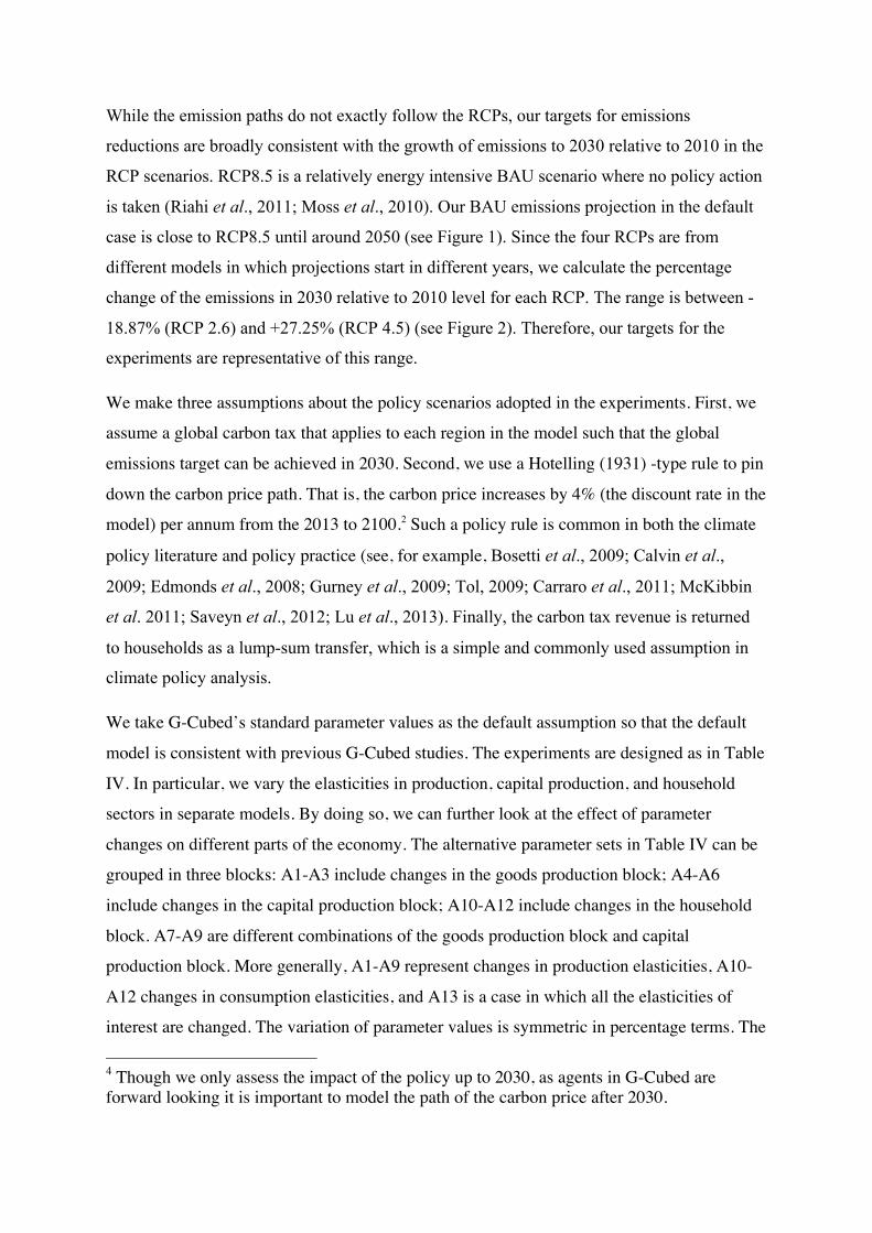
While the emission paths do not exactly follow the RCPs, our targets for emissions

reductions are broadly consistent with the growth of emissions to 2030 relative to 2010 in the

RCP scenarios. RCP8.5 is a relatively energy intensive BAU scenario where no policy action

is taken (Riahi et al., 2011; Moss et al., 2010). Our BAU emissions projection in the default

case is close to RCP8.5 until around 2050 (see Figure 1). Since the four RCPs are from

different models in which projections start in different years, we calculate the percentage

change of the emissions in 2030 relative to 2010 level for each RCP. The range is between -

18.87% (RCP 2.6) and +27.25% (RCP 4.5) (see Figure 2). Therefore, our targets for the

experiments are representative of this range.

We make three assumptions about the policy scenarios adopted in the experiments. First, we

assume a global carbon tax that applies to each region in the model such that the global

emissions target can be achieved in 2030. Second, we use a Hotelling (1931) -type rule to pin

down the carbon price path. That is, the carbon price increases by 4% (the discount rate in the

model) per annum from the 2013 to 2100.2 Such a policy rule is common in both the climate

policy literature and policy practice (see, for example, Bosetti et al., 2009; Calvin et al.,

2009; Edmonds et al., 2008; Gurney et al., 2009; Tol, 2009; Carraro et al., 2011; McKibbin

et al. 2011; Saveyn et al., 2012; Lu et al., 2013). Finally, the carbon tax revenue is returned

to households as a lump-sum transfer, which is a simple and commonly used assumption in

climate policy analysis.

We take G-Cubed’s standard parameter values as the default assumption so that the default

model is consistent with previous G-Cubed studies. The experiments are designed as in Table

IV. In particular, we vary the elasticities in production, capital production, and household

sectors in separate models. By doing so, we can further look at the effect of parameter

changes on different parts of the economy. The alternative parameter sets in Table IV can be

grouped in three blocks: A1-A3 include changes in the goods production block; A4-A6

include changes in the capital production block; A10-A12 include changes in the household

block. A7-A9 are different combinations of the goods production block and capital

production block. More generally, A1-A9 represent changes in production elasticities, A10-

A12 changes in consumption elasticities, and A13 is a case in which all the elasticities of

interest are changed. The variation of parameter values is symmetric in percentage terms. The

4 Though we only assess the impact of the policy up to 2030, as agents in G-Cubed are forward looking it is important to model the path of the carbon price after 2030.

range of ±50% will give us a good variation as the inputs in some sectors will turn from poor

(good) substitutes to good (poor) substitutes. To incorporate some insights from empirical

studies, we also test four special parameter sets. Table IV. “C” denotes Clements where all

the relevant elasticities of substitution are 0.5, as Clements (2008) suggested. “S” denotes

Stern where the top tier elasticities are 0.5 and the inter-fuel ones are 1, being generally

consistent with Stern’s (2012) estimates. Compared to the default model, the top-tier

elasticities are a bit tighter on average in the Clements assumption while the inter-fuel

substitution is a bit relaxed. The Stern assumption further relaxes the inter-fuel elasticities of

substitution. “EL” and “EH” denotes, respectively, “extremely low” where we assume all the

elasticities are only 0.1, and “extremely high” where all the elasticities are assumed to be 2.

These two parameter sets are unrealistic, but illustrate some extreme scenarios. We also ran

some models where we also restricted the elasticities of substitution that aggregate materials

into material bundles. The results were almost identical to the A13 scenario and so we do not

report these.

5. Results

5.1 Scenarios Using the Default Parameter Set

In the default parameter setting, the initial carbon taxes in 2013 range from $37 per tonne

($10 per tonne of CO2) to $63 per tonne ($17 per tonne of CO2) across the four policy

scenarios. Figure 3 compares the converted CO2 prices in 2020 in 2005 US dollars with the

prices simulated in EMF22 (Clarke et al., 2009). Our simulated carbon prices are within the

range of the carbon prices from the EMF22 scenarios.3 This indicates that our default results

are within a sensible range among the various models in this field.

Table V. summarizes the discounted cumulative GDP losses and cumulative emissions

reduction relative to BAU from 2013 to 2030 as well as the present value of average

abatement cost expressed in terms of loss of GDP per tonne of carbon abated. The average

abatement cost measured by is almost constant across the different scenarios, around

3 As most participating models failed to simulate the EMF22 450CO2-e scenario (comparable to RCP2.6), we compare our default carbon prices with the “Full participation and not-to-exceed” scenarios of 650CO2-e (comparable to RCP4.5) and 550CO2-e targets (comparable to a path somewhere between RCP2.6 and RCP4.5).

€

ΔGΔE

$103 per tonne of carbon. The GDP losses for each region and the world in 2030 relative to

BAU – how much lower GDP is in 2030, rather than the discounted sum of losses to 2030 -

are presented in Table VI. The cost, on both the regional and world level, decreases

consistently as the target becomes looser. As expected, costs are highest in energy exporting

developing countries (EEB and OPEC) and also in energy exporting developed countries

(Australia and Canada). Among other developed countries costs are highest in Japan and

lowest in the US, which is counter to the predictions of Stern et al. (2012) but may be

explained by tax interaction effects (Paltsev and Capros, 2013). As predicted by Stern et al.

(2012) costs are higher for developing countries than developed countries on the whole, but

again unexpectedly they are relatively low in India compared to China.

5.2 Factor Decomposition of GDP Losses Under Alternative Parameter Sets

We first present results for the world as a whole, and then do some comparisons across

regions.

(i) World Level

Table VII provides an overview of discounted GDP losses using each parameter set across

the four policy scenarios. The most noticeable features of these results are that changing the

parameters make little difference to the percentage GDP losses and that the A13 scenario

where all the relevant parameters are made less flexible has generally lower costs than the

other scenarios. Higher flexibility does not necessarily mean lower GDP losses relative to

BAU; on the contrary, in most cases, less flexible economies give us lower GDP losses

relative to BAU. The EL parameter set has the lowest costs of all. For Scenarios 3 and 4 the

carbon tax is in fact negative and so we have not reported a GDP loss. Decomposition

analysis can help explain this counter-intuitive result.

Figure 4 visualizes the decomposition in index form for the most and least stringent policy

scenarios and for more and less flexible (than the default) parameter sets in separate graphs.

To provide some intuition, a negative (positive) value for Δg implies that GDP losses are

lower (higher) with this parameter set than when using the default. From these results, we can

make several observations.

First, abatement costs per tonne of carbon are higher - positive ∆C - (lower) under the less

(more) flexible parameter sets while the amount of emissions to be abated is lower (higher).

However, the effect in terms of GDP losses (∆g) of changing elasticities of substitution in

different sectors (or blocks) is quite different depending on which elasticities are changed.

The effect of the elasticities in the capital producing sector (A4-A6) on GDP is negligible

while the effect is large in the goods production sectors (A1-A3). The impact of inter-fuel

substitution (A2) on the variation of GDP losses (∆g) is mainly due to the response of

average abatement cost (∆C) whereas the abatement factor (∆A) dominates the other factors

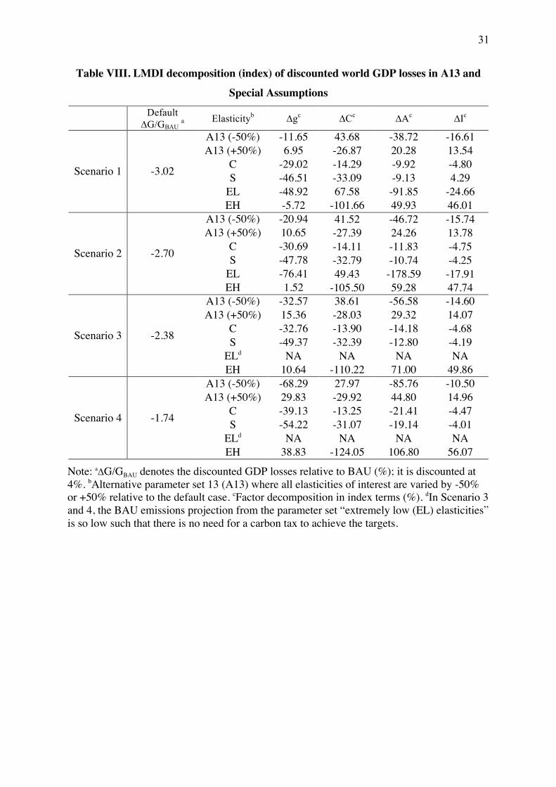
in the household consumption sector (A10). Furthermore, from Table VIII, we can see that as

policy scenarios become more stringent, the contribution from average abatement cost (∆C)

grows while the contribution from abatement (∆A) diminishes.

Second, comparing A1 with A2, and A10 with A11, we see that the top tier elasticities of

substitution have more impact on the average abatement cost (∆C) than inter-fuel elasticities

of substitution do in both the production and household sectors. This result is consistent with

Jacoby et al. (2006)’s finding that the elasticity of substitution between the energy and labor-

capital bundle turns out to be the most important parameter of those they test in terms of

welfare cost. Similarly, Babonneau et al. (2012) find that the top-tier elasticity has a greater

effect on the carbon price than the interfuel elasticity of substitution.

Third, the effect of changes in the elasticities of substitution on average abatement cost is not

symmetric. Generally a given percentage increase in flexibility leads to a smaller percentage

decrease in average abatement cost than the percentage increase in cost resulting from the

same percentage decrease in flexibility. This suggests that underestimation of elasticity

parameters in CGE models like G-Cubed will cause a greater bias in estimated abatement

cost than overestimation will. In short, it is clear that the top tier elasticity of substitution has

the largest impact on the average abatement cost and this impact is nonlinear. In terms of

total GDP losses relative to BAU, further factor decomposition is needed to distinguish what

drives the variation: whether it is from the changing average abatement cost in response to

policy shock or from the varying BAU scenario due to varied flexibility. There are also

different factors driving the results for different categories of elasticity of substitution.

Table VIII provides a closer look at the alternative parameter set A13 and the four special

parameter sets, where all the elasticities of interest are varied. In general, the Clements

assumption (C) and the Stern assumption (S) lead to lower mitigation cost, compared to the

default model. This suggests that relaxation of the elasticity of substitution in the electricity

sector (from 0.2) is more important than the tightening of the elasticities of substitution in

other sectors such as coal mining. The effects from the change in the BAU emission are very

similar for both parameter sets, and the major difference is the effect of average abatement

cost. This indicates that inter-fuel substitution has little impact on the BAU projection, but

significant impact on the average abatement cost. When the economy is highly inflexible

(EL) there is no need for mitigation policy under the less stringent targets. In fact, the optimal

carbon tax is negative. It is interesting to note that while the extreme elasticity assumptions

have a large impact on average abatement cost, they also have a significant impact on the

BAU projection.

(ii) Regional Comparison

In our experiments, there are important differences between the behavior of regions and

countries in the decomposition analysis. In the following analysis, we will compare some

representative regions/countries from different groups, specifically developed vs. developing

economies and energy importing vs. energy-exporting economies.

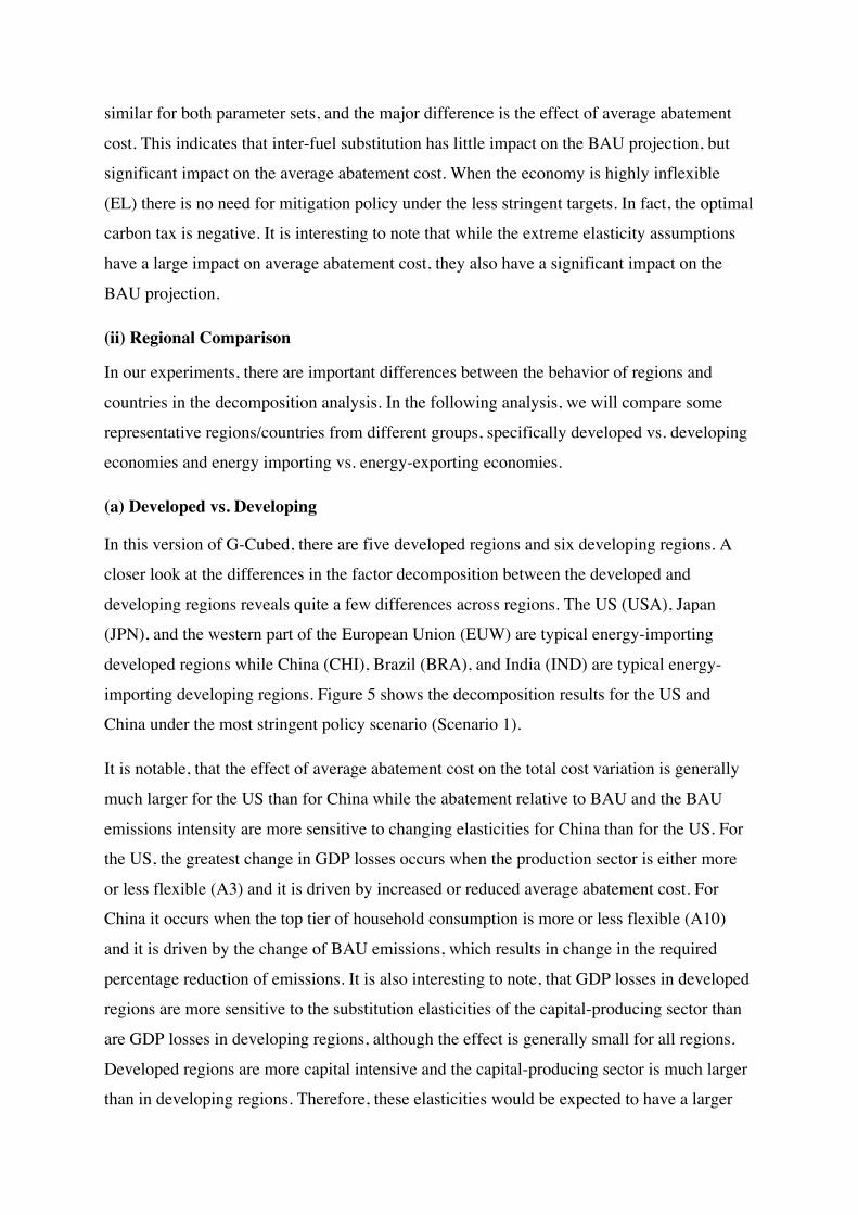
(a) Developed vs. Developing

In this version of G-Cubed, there are five developed regions and six developing regions. A

closer look at the differences in the factor decomposition between the developed and

developing regions reveals quite a few differences across regions. The US (USA), Japan

(JPN), and the western part of the European Union (EUW) are typical energy-importing

developed regions while China (CHI), Brazil (BRA), and India (IND) are typical energy-

importing developing regions. Figure 5 shows the decomposition results for the US and

China under the most stringent policy scenario (Scenario 1).

It is notable, that the effect of average abatement cost on the total cost variation is generally

much larger for the US than for China while the abatement relative to BAU and the BAU

emissions intensity are more sensitive to changing elasticities for China than for the US. For

the US, the greatest change in GDP losses occurs when the production sector is either more

or less flexible (A3) and it is driven by increased or reduced average abatement cost. For

China it occurs when the top tier of household consumption is more or less flexible (A10)

and it is driven by the change of BAU emissions, which results in change in the required

percentage reduction of emissions. It is also interesting to note, that GDP losses in developed

regions are more sensitive to the substitution elasticities of the capital-producing sector than

are GDP losses in developing regions, although the effect is generally small for all regions.

Developed regions are more capital intensive and the capital-producing sector is much larger

than in developing regions. Therefore, these elasticities would be expected to have a larger

effect on the economy in developed regions. These observations mostly hold for other

developed and developing regions too.

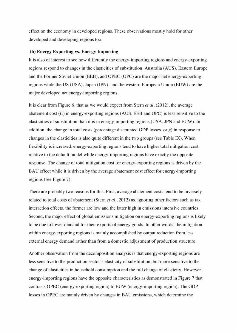
(b) Energy Exporting vs. Energy Importing It is also of interest to see how differently the energy-importing regions and energy-exporting

regions respond to changes in the elasticities of substitution. Australia (AUS), Eastern Europe

and the Former Soviet Union (EEB), and OPEC (OPC) are the major net energy-exporting

regions while the US (USA), Japan (JPN), and the western European Union (EUW) are the

major developed net energy-importing regions.

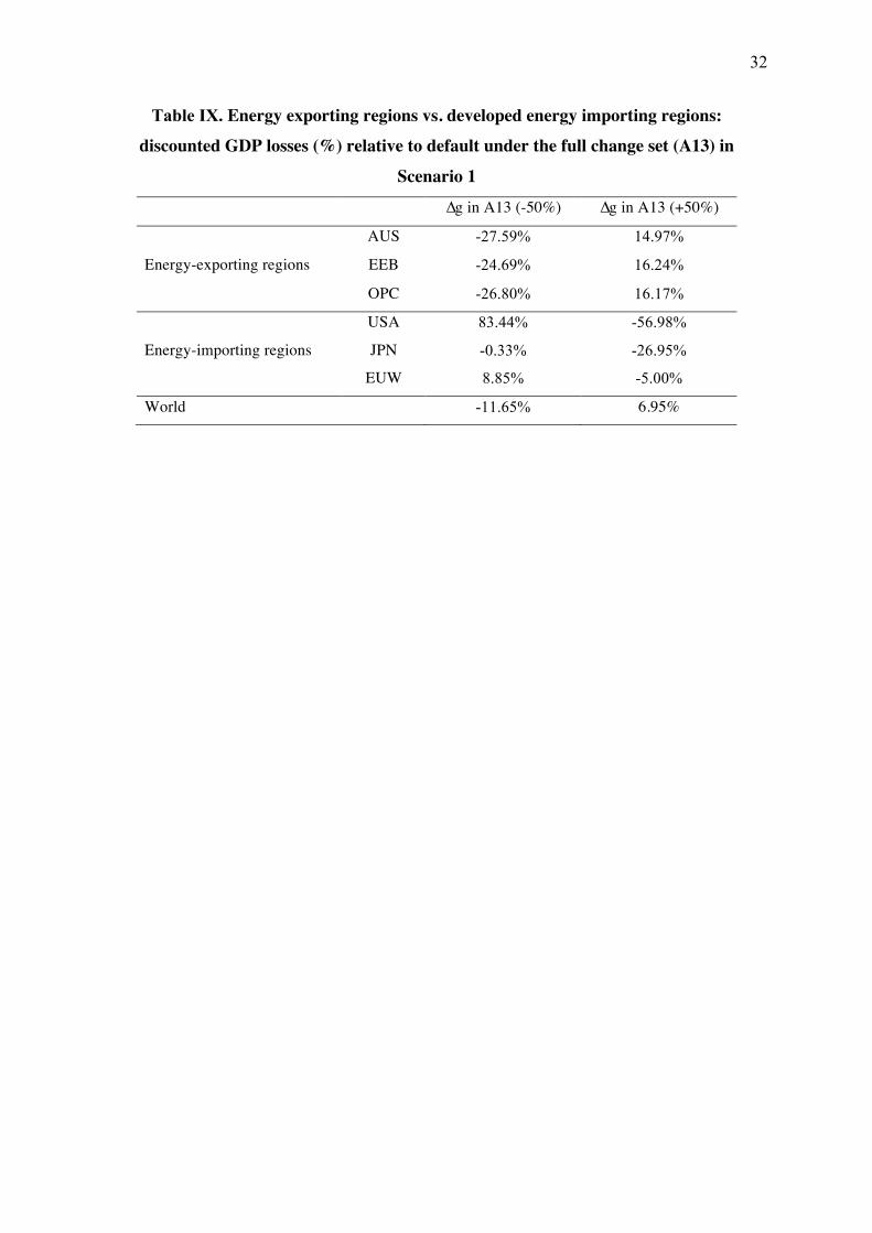
It is clear from Figure 6, that as we would expect from Stern et al. (2012), the average

abatement cost (C) in energy-exporting regions (AUS, EEB and OPC) is less sensitive to the

elasticities of substitution than it is in energy-importing regions (USA, JPN and EUW). In

addition, the change in total costs (percentage discounted GDP losses, or g) in response to

changes in the elasticities is also quite different in the two groups (see Table IX). When

flexibility is increased, energy-exporting regions tend to have higher total mitigation cost

relative to the default model while energy-importing regions have exactly the opposite

response. The change of total mitigation cost for energy-exporting regions is driven by the

BAU effect while it is driven by the average abatement cost effect for energy-importing

regions (see Figure 7).

There are probably two reasons for this. First, average abatement costs tend to be inversely

related to total costs of abatement (Stern et al., 2012) as, ignoring other factors such as tax

interaction effects, the former are low and the latter high in emissions intensive countries.

Second, the major effect of global emissions mitigation on energy-exporting regions is likely

to be due to lower demand for their exports of energy goods. In other words, the mitigation

within energy-exporting regions is mainly accomplished by output reduction from less

external energy demand rather than from a domestic adjustment of production structure.

Another observation from the decomposition analysis is that energy-exporting regions are

less sensitive to the production sector’s elasticity of substitution, but more sensitive to the

change of elasticities in household consumption and the full change of elasticity. However,

energy-importing regions have the opposite characteristics as demonstrated in Figure 7 that

contrasts OPEC (energy-exporting region) to EUW (energy-importing region). The GDP

losses in OPEC are mainly driven by changes in BAU emissions, which determine the

percentage abatement needed. Changes in BAU emissions intensity due to more or less

flexibility play a role in the EUW GDP losses, but the average abatement cost effect still

dominates. The flexibility in the household consumption bundle both at home and abroad

seems important to energy-exporting regions as it will largely affect the global energy

demand and through international trade, the net energy-exporters are affected more than

energy-importing regions by mitigation elsewhere.

6. Discussion and Conclusions

In this section, we compare our results with previous relevant studies, provide some general

conclusions, and then point out implications for future research and policy in this field.

Regarding average abatement costs, our results are qualitatively consistent with Jorgenson et

al. (2000) and Babonneau et al. (2012). The average cost of emissions reductions is generally

higher when substitution is more restricted. In the model where we change all elasticities of

substitution, A13, the average abatement cost at the world level increases (decreases) by 61%

(38%) if the world economy is 50% less (more) flexible compared to our base case. These

results also show the nonlinearity of average abatement cost in elasticities of substitution: the

average abatement cost increases more when the elasticities of substitution are lowered than

it decreases when the elasticities of substitution are increased by the same percentage. This

finding implies that overestimation of mitigation cost due to underestimating the elasticities

of substitution would be a more serious problem in CGE models than underestimation of cost

due to overestimating the elasticities of substitution. Similarly, Pindyck (2013) and N. Stern

(2013) argue that the benefits of climate policy have been underestimated because of

uncertainties in climate impact parameters in integrated assessment models. In particular, the

climate sensitivity to doubling carbon dioxide is uncertain more on the upper tail where

impacts are larger than on the lower tail where impacts are lower.

In common with Jacoby et al. (2006) and Babonneau et al. (2012), we find that average

abatement costs are generally more sensitive to changes in top tier (labor, capital, energy and

materials) substitution possibilities than to changes in inter-fuel substitution possibilities.

Changes in flexibility in the capital-producing sector are also important for developed

(capital-intensive) economies. For energy exporting regions, household consumption

substitution has a greater effect on total mitigation cost (GDP losses) than substitution in the

production sector; but the average abatement cost is more sensitive to substitution in the

production sector than in the household consumption sector. From our decomposition

analysis, we notice that changing the elasticity of substitution in consumption changes BAU

emissions a lot in these regions, but does not affect the average abatement cost much. This

may be because of G-Cubed’s assumption that carbon tax revenues are recycled by

transferring the revenue to households, who then spend some of this income on energy goods.

This offsets the reduction of household energy consumption due to an energy price rise

induced by a carbon tax.

We also find that inter-fuel substitution elasticities do have a significant impact on average

abatement cost, but not on BAU emissions. Top-tier (KLEM) elasticities of substitution

strongly affect BAU emissions. As predicted by de La Grandville (1989), less flexible

economies grow more slowly and as a result also have less emissions growth. The total costs

of mitigation are, therefore, lower in these economies than in more flexible economies. In our

extreme low flexibility parameter set (all relevant elasticities are 0.1), there is little GDP or

emissions growth at all, and no need for mitigation actions under the two less stringent policy

scenarios. As there is considerable growth in the real world this parameter set cannot be close

to reality.

Though we set out to test whether the costs of mitigation policies might be very high in less

flexible economies we found seemingly paradoxically that there is less need for climate

policy in such economies because emissions grow slower under BAU. In a sense Jackson

(2009) is correct that by stopping economic growth we eliminate the need for climate

mitigation, but this is achieved through the unrealistic and extremely expensive route of

making the economy less flexible. Under more realistic parameter sets there is a need for

climate mitigation but the costs are only a few percent of GDP at most.

Although the quantitative results in this study are derived from a particular model, the study,

in a broader sense, suggests that it is important to reduce the uncertainty regarding

substitution possibilities in climate policy assessment and to differentiate between the costs

of relative and absolute targets and between marginal, average, and total costs as already

argued by Stern et al. (2012). Our results show that, if we are interested in the total costs of

mitigation policy then accurate estimates of substitution elasticities are not that important. If

we are interested in marginal or average costs, then accurate parameter estimates are

important.

Our findings need to be taken into account when interpreting the results of model comparison

exercises. Most model comparisons, such as EMF22 (Clarke et al., 2009), show a wide range

of mitigation costs across models for common absolute targets. But each of these models has

a different BAU emissions projection. It is then important to identify whether the variation of

these mitigation costs is due to the varying BAU scenarios in each model or from the induced

costs of mitigation policy. Therefore, our study suggests that there is a necessity for

sensitivity and decomposition analysis to provide further policy recommendation using CGE

models.

References

Acemoglu, D., Aghion, P., Bursztyn, L., and Hemous, D. (2012) The Environment and Directed Technical Change. American Economic Review, 102(1): 131-166. Ang, B. W. (2004) Decomposition analysis for policymaking in energy: which is the preferred method? Energy Policy 32(9): 1131-1139.

Ang, B.W. and Liu, F.L. (2001) A New Energy Decomposition Method: Perfect in Decomposition and Consistent in Aggregation. Energy 26 (6): 537–548.

Babonneau, F., Haurie, A., Loulou, R., and Vielle, M. (2012) Combining Stochastic Optimization and Monte Carlo Simulation to Deal with Uncertainties in Climate Policy Assessment. Environmental Modeling & Assessment 17(1-2): 51-76.

Beckman, J. and Hertel, T. (2009) Why Previous Estimates of the Cost of Climate Mitigation are Likely Too Low. GTAP Working Papers 2954.

Bhattacharya, S. C. (1996) Applied General Equilibrium Models for Energy Studies. Energy Economics 18: 145-164.

Bossetti, V., Carraro, C., De Cian, E., Duval, R., Massetti, E., and Tavoni, M. (2009) The Incentives to Participate in and the Stability of International Climate Coalitions: A Game-Theoretic Approach Using the WITCH Model. OECD Economics Department Working Papers 702, OECD Publishing.

Boyd, O. (2012) China's Energy Reform and Climate Policy: The Ideas Motivating Change. CCEP Working Paper 1205.

Calvin, K., Patel, P., Fawcett, A., Clarke, L., Fisher-Vanden, K., Edmonds, J., Kim, S. H., Sands, S., and Wise, M. (2009) The Distribution and Magnitude of Emissions Mitigation Costs in Climate Stabilization under Less than Perfect International Cooperation: SGM Results. Energy Economics 31 (Supplement 2): S187-S197.

Carraro, C. and Massetti, E. (2011). Energy and Climate Change in China. FEEM Working Paper 16.2011.

Clarke, L., Edmonds, J., Krey, V.C., Richels, R., Rose, S., and Tavoni, M. (2009). International Climate Policy Architectures: Overview of the EMF 22 International Scenarios. Energy Economics 31(Supplement 2): S64-S81.

Clements, K. W. (2008) Price Elasticities of Demand are Minus One-Half. Economics Letters 99(3): 490-493.

Dietz, S. and Stern, N. (2008) Why Economic Analysis Supports Strong Action on Climate Change: A Response to the Stern Review’s Critics. Review of Environmental Economics and Policy 2(1): 94–113.

Edmonds, J., Clarke, L., Lurz, J., and Wise, M. (2008). Stabilizing CO2 Concentrations with Incomplete International Cooperation. Climate Policy 8: 355–376.

Garnaut, R. (2008) The Garnaut Climate Change Review: Final Report. Cambridge University Press.

Goulder, L.H. and Williams, R.C. (2012) The Choice of Discount Rate for Climate Change Policy Evaluation. Climate Change Economics 03: 1250024.

Goettle, R. J., Ho, M. S., Jorgenson, D. W., Slesnick, D. T., and Wilcoxen, P. J. (2007) IGEM, an Inter-temporal General Equilibrium Model of the U.S. Economy with Emphasis on Growth, Energy and the Environment. Prepared for the U.S. Environmental Protection Agency (EPA), Office of Atmospheric Programs, Climate Change Division.

Gurney, A., Ahammad, H., and Ford, M. (2009) The Economics of Greenhouse Gas Mitigation: Insights from Illustrative Global Abatement Scenarios Modeling. Energy Economics 31(Supplement 2): S174-S186.

Hotelling, H. (1931) The Economics of Exhaustible Resources. Journal of Political Economy 39: 137–175.

Hourcade, J-C., Pottier, A., and Espagne, E. (2011) The Environment and Directed Technical Change: Comment. Fondazione Eni Enrico Mattei Working Papers 646.

Houser, T., Bradley, R., Childs, B., Werksman, J., and Heilmayr, R. (2008) Leveling the Carbon Playing Field: International Competition and US Climate Policy Design. Peterson Institute of International Economics/World Resources Institute, Washington DC.

Jackson, T. (2009) Prosperity without Growth: Economics for a Finite Planet. Earthscan.

Jorgenson, D. W., Goettle, R. J., Wilcoxen, P. J., and Ho, M. S. (2000) The Role of Substitution in Understanding the Costs of Climate Change Policy. Report prepared for the Pew Center on Global Climate Change.

Jacoby, H. D., Reilly, J. M, McFarland, J. R., and Paltsev, S. (2006) Technology and Technical Change in the MIT EPPA Model. Energy Economics 28(5-6): 610-631.

Kennedy, A. B. (2013) China’s Search for Renewable Energy: Pragmatic Techno-nationalism. Asian Survey 53(5): 909-930.

Koetse, M. J., de Groot, H. L. F., and Florax, R. J. G. M. (2008) Capital-Energy Substitution and Shifts in Factor Demand: A Meta-Analysis. Energy Economics 30: 2236–2251.

de La Grandville, O. (1989) In Quest of the Slutsky Diamond. American Economic Review 79(3): 468-481.

Lu, Y., Stegman, A., and Cai, Y. (2013) Emissions Intensity Targeting: From China's 12th Five Year Plan to Its Copenhagen Commitment. Energy Policy 61: 1164-1177.

McKibbin, W. J. and Wilcoxen, P. J. (1999) The Theoretical and Empirical Structure of the G-Cubed Model, Economic Modelling 16: 123-148.

McKibbin, W. J. and Wilcoxen, P. J. (2013) A Global Approach to Energy and the Environment: The G-Cubed Model. In: P. B. Dixon and D. W. Jorgenson (eds.) Handbook of Computable General Equilibrium Modeling. Elsevier: 995-1068.

McKibbin, W. J., Wilcoxen, P. J. and Woo, W. T. (2008) China Can Grow and Still Help Prevent the Tragedy of the Carbon Dioxide Commons. CAMA Working Paper 14/2008.

McKibbin, W. J., Ross, M. T., Shackleton, R., Wilcoxen, P. J. (1999) Emissions Trading, Capital Flows and the Kyoto Protocol. Energy Journal Special Issue: The Costs of the Kyoto Protocol: 287-334.

McKibbin, W. J., Morris, A. C. and Wilcoxen, P. J. (2011) Comparing Climate Commitments: A Model-based Analysis of the Copenhagen Accord. Climate Change Economics 2: 79–103.

Moss, R. H., Edmonds, J. A., Hibbard, K. A., Manning, M. R., Rose, S. K., van Vuuren, D. P., Carter, T. R., Emori, S., Kainuma, M., Kram, T., Meehl, G. A., Mitchell, J. F., Nakicenovic, N., Riahi, K., Smith, S. J., Stouffer, R. J., Thomson, A. M., Weyant, J. P., and Wilbanks, T. J. (2010) The Next Generation of Scenarios for Climate Change Research and Assessment. Nature 463(7282): 747-756.

Nordhaus, W. (2007) A Review of the Stern Review on the Economics of Climate Change. Journal of Economic Literature 45: 686-702.

Paltsev, S. and Capros, P. (2013) Cost Concepts for Climate Mitigation. Climate Change Economics 4: 1340003.

Pezzey, J. C. V. and Lambie, N. R. (2001) CGE Models for Evaluating Domestic Greenhouse Policies in Australia: A Comparative Analysis. Consultancy Report for the Productivity Commission.

Pindyck, R. (2013) Climate Change Policy: What Do the Models Tell Us? Journal of Economic Literature 51(3): 860–872.

Riahi, K., Rao, S., Krey, V., Cho, C., Chirkov, V., Fischer, G., Kindermann, G., Nakicenovic, N., and Rafai, P. (2011) RCP 8.5—A Scenario of Comparatively High Greenhouse Gas Emissions. Climatic Change 109: 33-57.

Saunders, H. D. (1992) The Khazzoom-Brookes Postulate and Neoclassical Growth. Energy Journal 13(4): 131-148.

Saveyn, B., Paroussos, L., and Ciscar, J.-C. (2012) Economic Analysis of a Low Carbon Pathway to 2050: A Case for China, India and Japan. Energy Economics 34(Supplement 3): S451-S458.

Stern, D. I. (2012) Interfuel Substitution: A Meta-analysis. Journal of Economic Surveys 26(2): 307-331.

Stern, D. I., Pezzey, J. C. V., and Lambie, N. R. (2012) Where in the World is it Cheapest to Cut Carbon Emissions? Australian Journal of Agricultural and Resource Economics 56(3): 315-331.

Stern, N. H. (2007) The Economics of Climate Change: The Stern Review. Cambridge and New York: Cambridge University Press.

Stern, N. H. (2013) The Structure of Economic Modeling of the Potential Impacts of Climate Change: Grafting Gross Underestimation of Risk onto Already Narrow Science Models. Journal of Economic Literature 51(3): 838-859.

Sunstein, C. R. (2007-2008) The World vs. The United States and China - The Complex Climate Change Incentives of the Leading Greenhouse Gas Emitters. UCLA Law Review 55(6): 1675-1700.

Tavoni, M. and Tol, R. S. J. (2010) Counting Only the Hits? The Risk of Underestimating the Costs of a Stringent Climate Policy. Climatic Change 100: 769–778.

Tol, R. S. J. (2009) The Feasibility of Low Concentration Targets: An Application of FUND. Energy Economics 31(Supplement 2): S121-S130.

Tol, R. S. J. (2011) Modified Ramsey Discounting for Climate Change. ESRI Working Paper 368.

Treasury (2008) Australia’s Low Pollution Future: The Economics of Climate Change Mitigation. Commonwealth of Australia.

van Vuuren, D. P., Edmonds, J., Kainuma, M., Riahi, K., Thomson, A., Hibbard, K., Hurtt, G. C., Kram, T., Krey, V., Lamarque, J.-F., Masui, T., Meinshausen, M., Nakicenovic, N., Smith, S. J., and Rose, S. K. (2011) The Representative Concentration Pathways: An Overview. Climatic Change 109(1-2): 5-31.

Webster, M., Sokolov, A., Reilly, J., Forest, C., Paltsev, S., Schlosser, A., Wang, C., Kicklighter, D., Sarofim, M., Melillo, J., Prinn, R., and Jacoby, H. (2012) Analysis of Climate Policy Targets under Uncertainty. Climatic Change 112(3-4): 569-583.

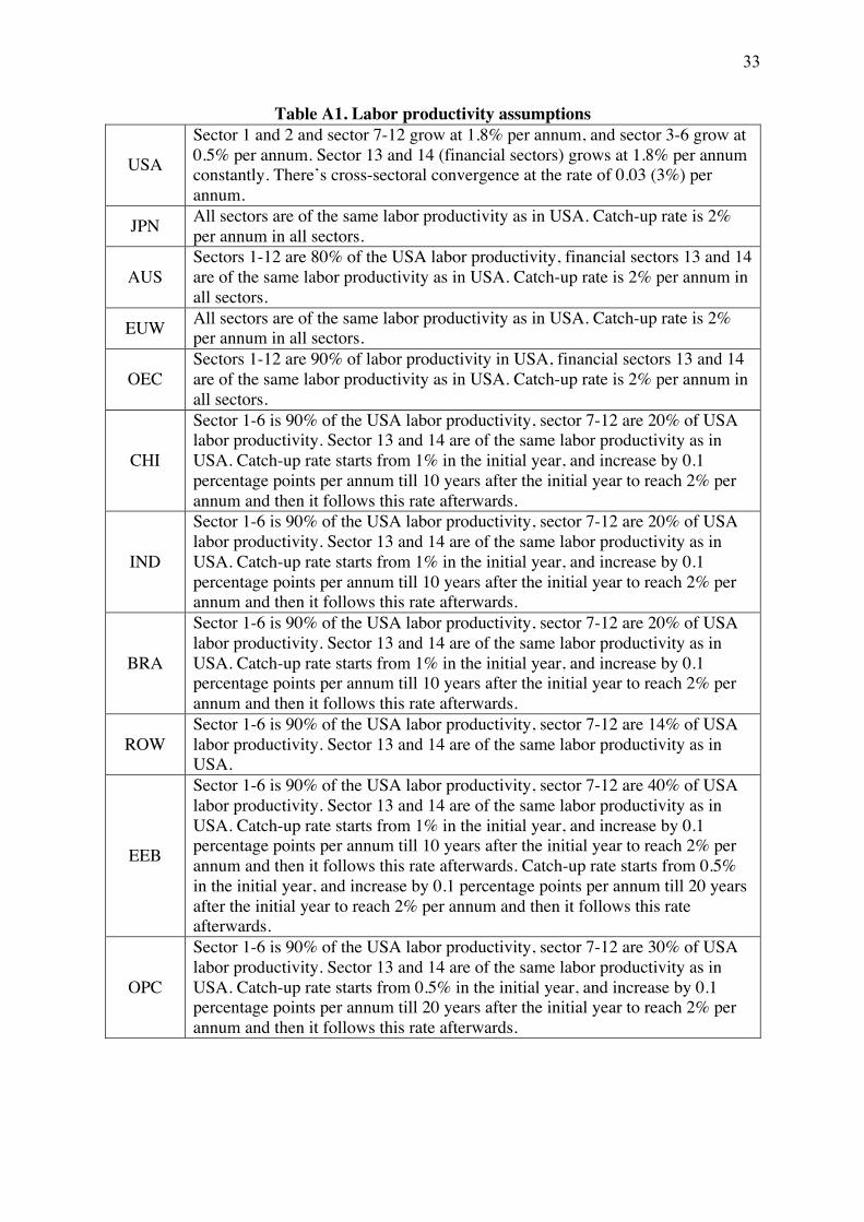
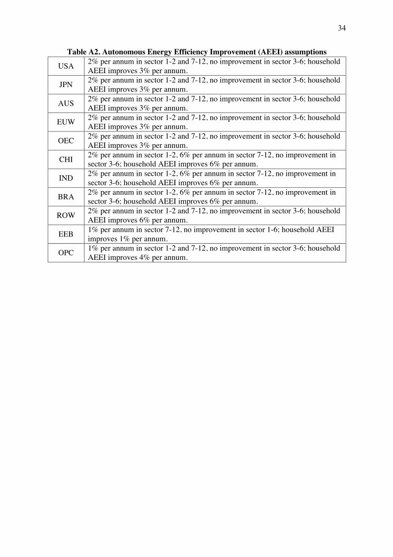
Appendix A: Technological Change Assumptions

Tables A1 and A2 present the assumptions on the rates of technological changed used in this

study.

Appendix B: The Structure of The G-Cubed Model

We use G-Cubed to test the sensitivity of mitigation costs in a computable general

equilibrium model to changes in the elasticity of substitution parameters. G-Cubed has some

important features that serve this purpose. G-Cubed has various tiers of nesting on the

production and consumption sides, which allows us to explore the substitutability of the

economy at different levels (see Figure A1). In the following, we describe the features of the

model that are most relevant to our sensitivity analysis. McKibbin and Wilcoxen (1999,

2013) provide a more complete description of the model. There are twelve production sectors

where the top tier level of production is modeled as a CES function of capital, labor, energy

and materials:

(A1)

where Qi is the output for sector i, Xij is the inputs for sector i; AiO, σi

O and δijO are parameters

that reflect technology, elasticity of substitution, and input weights, respectively. Particularly,

AjO (j=K,L,E,M) is the factor-specific technology parameter at the top tier. The energy (XiE)

and materials (XiM) inputs in (1) are also modeled as CES functions of component energy

carriers and materials:

(A2)

where X,iE is the aggregate energy used in sector i. The XijE represent outputs of the six

energy producing sectors including: electricity, crude oil, coal, petroleum, natural gas and its

utility; σiE and δij

E are inter-fuel elasticity and input weights parameters, respectively.

Similarly the aggregate material input is a CES aggregate of the outputs from the six

“materials” producing sectors of the economy. Materials in fact include transportation and

services inputs. Each of these lower tier inputs – both materials and energy - are a CES

aggregate of domestic and imported commodities where the elasticity of substitution is the

Armington elasticity.

In addition to the twelve ordinary industrial sectors, there are also a capital goods production

sector, which has a similar nesting, with σOR and σER being the elasticity parameters in the

two tiers.4

On the household side, the representative household utility function is given by:

∫∞

−−+=t

tst dsesGsCU )())(ln)((ln θ (A3)

4 There is also a household capital producing sector in a similar nesting; but the elasticity of substitution is not of interest here in this study.

1

,,,

11

)()(−

=

−

⎟⎟⎟

⎠

⎞

⎜⎜⎜

⎝

⎛= ∑

Oi

Oi

Oi

Oi

Oi

MELKjij

Oj

Oij

Oii XAAQ

σ

σ

σ

σ

σδ

1

6,..,1

11

)(−

=

−

⎟⎟

⎠

⎞

⎜⎜

⎝

⎛= ∑

Ei

Ei

Ei

EiE

i

j

Eij

EijiE XX

σ

σ

σ

σσδ

where C is aggregate consumption and G is government consumption, which is intended to

measure the provision of public goods; θ is the rate of pure time preference. Aggregate

consumption C also has two layers of CES nesting: one is the top tier nesting of household

capital, labor, energy, and materials; the lower tier consists of inter-fuel nesting for energy

(with elasticity σEH) and nesting for material goods (with elasticity σMH). Therefore, the top

tier consumption aggregate is as follows:

(A4)

in which σCO (or σOH in the model codes) and δCj are elasticity of substitution between 12

consumption goods and the corresponding weights parameters, respectively. The elasticities:

σiO, σi

E, σOR, σER, σOH and σEH are the parameters of interest in our sensitivity analysis.

The G-Cubed model also features macro-economic characteristics such as partly rational

expectations, price stickiness, and a central bank policy rule. These distinctive features that

most recursive CGE models do not have, give the model rich short-run dynamics and make

the model more suitable for short to medium term scenario analysis. While long-run

consequences are the usual focus of climate scientists, the short-run to medium run (two to

three decades) dynamics are probably more relevant to policy-makers and economists. G-

Cubed also features a comprehensive representation of international trade, which is important

for issues in a global context, like climate change.

1

,,,

11

)(−

=

−

⎟⎟

⎠

⎞

⎜⎜

⎝

⎛= ∑

OC

OC

OC

OC

OC

MELKjCj

CCj XC

σ

σ

σ

σ

σδ

Table I. Regional aggregation of the model (G-Cubed, version D) Region Name Region Code Region Description USA USA United States Japan JPN Japan Australia AUS Australia Europe EUW European Union Rest of the Advanced Economies

OEC Canada and New Zealand

China CHI China India IND India Brazil BRA Brazil OPEC OPC Oil Exporting and other Middle Eastern

Countries EEFSU EEB Eastern Europe and the former Soviet

Union ROW ROW Rest of the World

Table II. Sector aggregation in the model (G-Cubed, version D)

Number Sector Definition 1 Electric Utilities 2 Gas Utilities 3 Petroleum Refining 4 Coal Mining 5 Crude Oil Extraction 6 Gas Extraction 7 Mining 8 Agriculture, Forestry, Fishing and

Hunting 9 Durable Manufacturing 10 Non-Durable Manufacturing 11 Transportation 12 Services 13 Capital Producing Sector 14 Household Capital Producing

Sector

Table III. Key elasticities of substitution in G-Cubed

Sectors Top tier (O) Energy tier (E)

σi (i=O, E)

1. Electric utilities 0.20 0.20 2. Gas utilities 0.81 0.50 3. Petroleum refining 0.54 0.20 4. Coal mining 1.70 0.16 5. Crude oil extraction 0.49 0.14 6. Gas extraction 0.49 0.14 7. Mining 1.00 0.50 8. Agriculture, forestry, fishing and hunting 1.28 0.50

9. Durable manufacturing 0.41 0.50 10. Non-durable manufacturing 0.5 0.50 11. Transportation 0.54 0.50 12. Services 0.26 0.32

σiR (i=O, E) Capital producing sector 1.10 0.5 σiH (i=O, E) Household consumption 0.8 0.5

Note: O denotes the top tier nesting between Capital (K), Labor (L), Energy (E) and Materials (M). E denotes the energy level nesting between the 6 energy goods corresponding to the first 6 sectors in Table II.

28 Table IV. Simulation experiments design

Default Variations Alternative Parameter Sets Special Assumptions +50% -50% A1 A2 A3 A4 A5 A6 A7 A8 A9 A10 A11 A12 A13 C S EL EH

S 1 0.20 0.30 0.10 X X X X X

0.5

0.5

0.1 2

S 2 0.81 1.21 0.41 X X X X X S 3 0.54 0.81 0.27 X X X X X S 4 1.70 2.56 0.85 X X X X X S 5 0.49 0.74 0.25 X X X X X S 6 0.49 0.74 0.25 X X X X X S 7 1.00 1.50 0.50 X X X X X S 8 1.28 1.93 0.64 X X X X X S 9 0.41 0.62 0.21 X X X X X

S 10 0.50 0.75 0.25 X X X X X S 11 0.54 0.81 0.27 X X X X X S 12 0.26 0.38 0.13 X X X X X

S 1 0.20 0.30 0.10 X X X X X

1

S 2 0.50 0.75 0.25 X X X X X S 3 0.20 0.30 0.10 X X X X X S 4 0.16 0.24 0.08 X X X X X S 5 0.14 0.21 0.07 X X X X X S 6 0.14 0.21 0.07 X X X X X S 7 0.50 0.75 0.25 X X X X X S 8 0.50 0.75 0.25 X X X X X S 9 0.50 0.75 0.25 X X X X X

S 10 0.50 0.75 0.25 X X X X X S 11 0.50 0.75 0.25 X X X X X S 12 0.32 0.48 0.16 X X X X X

1.10 1.65 0.55 X X X X X 0.5

0.50 0.75 0.25 X X X X X 1

0.80 1.20 0.40 X X X 0.5

0.50 0.75 0.25 X X X 1 Note: (1) “X” indicates a change of parameter value from the default case. (2) “S+ a number from 1 to 12” in Column 2 corresponds to sector number as shown in Table II

!

" o

eσ

oRσ

eRσ

oHσ

eHσ

29

Table V. Global discounted GDP losses and cumulative emissions abatement

Policy Scenario

World Discounted GDP Losses World Cumulative Abatement World Average Cost (2010

USD/tonne of carbon)

Absolute value (Trillions of 2010

USD)

Percentage (%)

Absolute value (Billions of tonnes of

carbon)

Percentage (%)

Scenario 1 (Target 1) -34.0 -3.02 -329.1 -41.76 103.35

Scenario 2 (Target 2) -30.4 -2.70 -294.3 -37.34 103.29

Scenario 3 (Target 3) -26.8 -2.38 -259.5 -32.93 103.24

Scenario 4 (Target 4) -19.6 -1.74 -190.1 -24.12 103.14

Note: GDP losses are net present value discounted at 4% per year.

Table VI. GDP losses (%) in 2030 for the four scenarios relative to BAU

Scenario 1

Scenario 2

Scenario 3

Scenario 4

USA -1.28 -1.22 -1.14 -0.93 JPN -4.30 -3.97 -3.61 -2.80 AUS -4.50 -4.00 -3.51 -2.54 EUW -2.68 -2.47 -2.24 -1.74 OEC -4.36 -3.92 -3.47 -2.57 CHI -6.28 -5.39 -4.56 -3.04 IND -1.98 -1.68 -1.40 -0.91 BRA -0.99 -0.92 -0.85 -0.68 ROW -5.98 -5.37 -4.76 -3.52 EEB -10.62 -9.35 -8.12 -5.77 OPC -12.71 -11.32 -9.94 -7.22

World -4.20 -3.76 -3.32 -2.44

30

Table VII. Discounted GDP losses (%) on the world level using different parameter sets

Scenario 1 Scenario 2 Scenario 3 Scenario 4 Default -3.02 -2.70 -2.38 -1.74

Panel A: Less flexible by 50% A1 -3.02 -2.62 -2.23 -1.44 A2 -3.33 -2.97 -2.62 -1.92 A3 -3.34 -2.99 -2.54 -1.64 A4 -2.96 -2.64 -2.31 -1.67 A5 -3.02 -2.70 -2.38 -1.74 A6 -2.96 -2.64 -2.32 -1.68 A7 -2.92 -2.52 -2.12 -1.32 A8 -3.33 -2.97 -2.62 -1.92 A9 -3.34 -2.88 -2.42 -1.52 A10 -2.56 -2.21 -1.87 -1.19 A11 -3.06 -2.73 -2.41 -1.76 A12 -2.59 -2.24 -1.89 -1.19 A13 -2.67 -2.13 -1.60 -0.55

Panel B: More flexible by 50% A1 -3.09 -2.82 -2.54 -2.00 A2 -2.77 -2.47 -2.18 -1.60 A3 -2.87 -2.62 -2.36 -1.85 A4 -3.00 -2.68 -2.36 -1.72 A5 -3.02 -2.70 -2.38 -1.74 A6 -3.00 -2.68 -2.36 -1.72 A7 -3.27 -3.00 -2.72 -2.17 A8 -2.77 -2.47 -2.18 -1.59 A9 -2.96 -2.71 -2.45 -1.94 A10 -3.41 -3.11 -2.81 -2.21 A11 -2.98 -2.67 -2.35 -1.73 A12 -3.37 -3.07 -2.78 -2.19 A13 -3.23 -2.99 -2.74 -2.26

Special Assumptions C -2.14 -1.87 -1.60 -1.06 S -1.62 -1.41 -1.20 -0.80

EL -1.54 -0.64 NA NA EH -2.85 -2.74 -2.63 -2.42

31

Table VIII. LMDI decomposition (index) of discounted world GDP losses in A13 and

Special Assumptions

Default ∆G/GBAU a Elasticityb ∆gc ∆Cc ∆Ac ∆Ic

Scenario 1 -3.02

A13 (-50%) -11.65 43.68 -38.72 -16.61 A13 (+50%) 6.95 -26.87 20.28 13.54

C -29.02 -14.29 -9.92 -4.80 S -46.51 -33.09 -9.13 4.29

EL -48.92 67.58 -91.85 -24.66 EH -5.72 -101.66 49.93 46.01

Scenario 2 -2.70

A13 (-50%) -20.94 41.52 -46.72 -15.74 A13 (+50%) 10.65 -27.39 24.26 13.78

C -30.69 -14.11 -11.83 -4.75 S -47.78 -32.79 -10.74 -4.25

EL -76.41 49.43 -178.59 -17.91 EH 1.52 -105.50 59.28 47.74

Scenario 3 -2.38

A13 (-50%) -32.57 38.61 -56.58 -14.60 A13 (+50%) 15.36 -28.03 29.32 14.07

C -32.76 -13.90 -14.18 -4.68 S -49.37 -32.39 -12.80 -4.19

ELd NA NA NA NA EH 10.64 -110.22 71.00 49.86

Scenario 4 -1.74

A13 (-50%) -68.29 27.97 -85.76 -10.50 A13 (+50%) 29.83 -29.92 44.80 14.96

C -39.13 -13.25 -21.41 -4.47 S -54.22 -31.07 -19.14 -4.01

ELd NA NA NA NA EH 38.83 -124.05 106.80 56.07

Note: a∆G/GBAU denotes the discounted GDP losses relative to BAU (%); it is discounted at 4%. bAlternative parameter set 13 (A13) where all elasticities of interest are varied by -50% or +50% relative to the default case. cFactor decomposition in index terms (%). dIn Scenario 3 and 4, the BAU emissions projection from the parameter set “extremely low (EL) elasticities” is so low such that there is no need for a carbon tax to achieve the targets.

32

Table IX. Energy exporting regions vs. developed energy importing regions: discounted GDP losses (%) relative to default under the full change set (A13) in

Scenario 1 ∆g in A13 (-50%) ∆g in A13 (+50%)

Energy-exporting regions

AUS -27.59% 14.97%

EEB -24.69% 16.24%

OPC -26.80% 16.17%

Energy-importing regions

USA 83.44% -56.98%

JPN -0.33% -26.95%

EUW 8.85% -5.00%

World -11.65% 6.95%

33

Table A1. Labor productivity assumptions

USA

Sector 1 and 2 and sector 7-12 grow at 1.8% per annum, and sector 3-6 grow at 0.5% per annum. Sector 13 and 14 (financial sectors) grows at 1.8% per annum constantly. There’s cross-sectoral convergence at the rate of 0.03 (3%) per annum.

JPN All sectors are of the same labor productivity as in USA. Catch-up rate is 2% per annum in all sectors.

AUS Sectors 1-12 are 80% of the USA labor productivity, financial sectors 13 and 14 are of the same labor productivity as in USA. Catch-up rate is 2% per annum in all sectors.

EUW All sectors are of the same labor productivity as in USA. Catch-up rate is 2% per annum in all sectors.

OEC Sectors 1-12 are 90% of labor productivity in USA, financial sectors 13 and 14 are of the same labor productivity as in USA. Catch-up rate is 2% per annum in all sectors.

CHI

Sector 1-6 is 90% of the USA labor productivity, sector 7-12 are 20% of USA labor productivity. Sector 13 and 14 are of the same labor productivity as in USA. Catch-up rate starts from 1% in the initial year, and increase by 0.1 percentage points per annum till 10 years after the initial year to reach 2% per annum and then it follows this rate afterwards.

IND

Sector 1-6 is 90% of the USA labor productivity, sector 7-12 are 20% of USA labor productivity. Sector 13 and 14 are of the same labor productivity as in USA. Catch-up rate starts from 1% in the initial year, and increase by 0.1 percentage points per annum till 10 years after the initial year to reach 2% per annum and then it follows this rate afterwards.

BRA

Sector 1-6 is 90% of the USA labor productivity, sector 7-12 are 20% of USA labor productivity. Sector 13 and 14 are of the same labor productivity as in USA. Catch-up rate starts from 1% in the initial year, and increase by 0.1 percentage points per annum till 10 years after the initial year to reach 2% per annum and then it follows this rate afterwards.

ROW Sector 1-6 is 90% of the USA labor productivity, sector 7-12 are 14% of USA labor productivity. Sector 13 and 14 are of the same labor productivity as in USA.

EEB

Sector 1-6 is 90% of the USA labor productivity, sector 7-12 are 40% of USA labor productivity. Sector 13 and 14 are of the same labor productivity as in USA. Catch-up rate starts from 1% in the initial year, and increase by 0.1 percentage points per annum till 10 years after the initial year to reach 2% per annum and then it follows this rate afterwards. Catch-up rate starts from 0.5% in the initial year, and increase by 0.1 percentage points per annum till 20 years after the initial year to reach 2% per annum and then it follows this rate afterwards.

OPC

Sector 1-6 is 90% of the USA labor productivity, sector 7-12 are 30% of USA labor productivity. Sector 13 and 14 are of the same labor productivity as in USA. Catch-up rate starts from 0.5% in the initial year, and increase by 0.1 percentage points per annum till 20 years after the initial year to reach 2% per annum and then it follows this rate afterwards.

34

Table A2. Autonomous Energy Efficiency Improvement (AEEI) assumptions

USA 2% per annum in sector 1-2 and 7-12, no improvement in sector 3-6; household AEEI improves 3% per annum.

JPN 2% per annum in sector 1-2 and 7-12, no improvement in sector 3-6; household AEEI improves 3% per annum.

AUS 2% per annum in sector 1-2 and 7-12, no improvement in sector 3-6; household AEEI improves 3% per annum.

EUW 2% per annum in sector 1-2 and 7-12, no improvement in sector 3-6; household AEEI improves 3% per annum.

OEC 2% per annum in sector 1-2 and 7-12, no improvement in sector 3-6; household AEEI improves 3% per annum.

CHI 2% per annum in sector 1-2, 6% per annum in sector 7-12, no improvement in sector 3-6; household AEEI improves 6% per annum.

IND 2% per annum in sector 1-2, 6% per annum in sector 7-12, no improvement in sector 3-6; household AEEI improves 6% per annum.

BRA 2% per annum in sector 1-2, 6% per annum in sector 7-12, no improvement in sector 3-6; household AEEI improves 6% per annum.

ROW 2% per annum in sector 1-2 and 7-12, no improvement in sector 3-6; household AEEI improves 6% per annum.

EEB 1% per annum in sector 7-12, no improvement in sector 1-6; household AEEI improves 1% per annum.

OPC 1% per annum in sector 1-2 and 7-12, no improvement in sector 3-6; household AEEI improves 4% per annum.

35

Figure 1. RCPs and G-Cubed BAU emissions paths (2010-2050)

Figure 2. RCPs and emissions targets (percentage relative to 2010 level)

0

10000

20000

30000

40000

50000

60000

70000

80000

90000

2010

2012

2014

2016

2018

2020

2022

2024

2026

2028

2030

2032

2034

2036

2038

2040

2042

2044

2046

2048

2050

Million  tons  of  C

O2

RCP2.6 RCP4.5 RCP6 RCP8.5 G-­‐Cubed  default  BAU

-­‐100%

-­‐50%

0%

50%

100%

150%

2010 2020 2030 2040 2050 2060

RCP2.6 RCP4.5 RCP6 RCP8.5

Target  1 Target  2 Target  3 Target  4

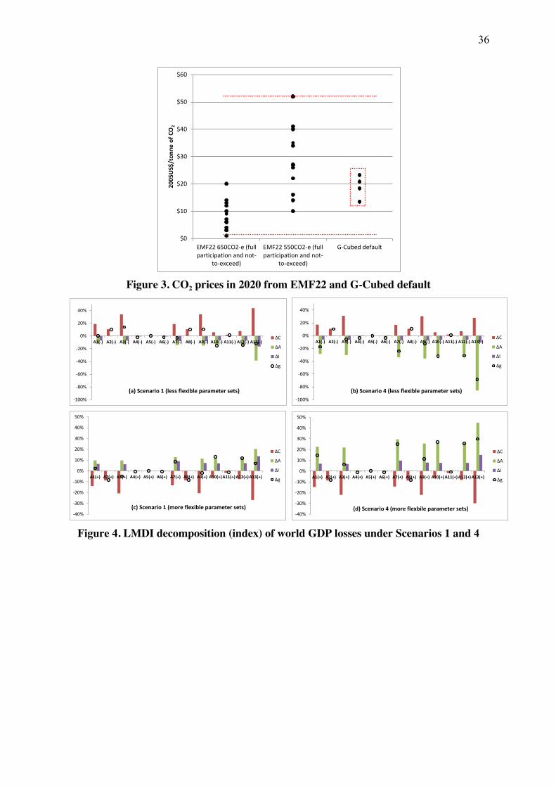
36

Figure 3. CO2 prices in 2020 from EMF22 and G-Cubed default

Figure 4. LMDI decomposition (index) of world GDP losses under Scenarios 1 and 4

$0

$10

$20

$30

$40

$50

$60

EMF22  650CO2-­‐e  (fullparticipation  and  not-­‐

to-­‐exceed)

EMF22  550CO2-­‐e  (fullparticipation  and  not-­‐

to-­‐exceed)

G-­‐Cubed  default

2005US$/ton

ne  of  C

O2

-­‐100%

-­‐80%

-­‐60%

-­‐40%

-­‐20%

0%

20%

40%

A1(-­‐) A2(-­‐) A3(-­‐) A4(-­‐) A5(-­‐) A6(-­‐) A7(-­‐) A8(-­‐) A9(-­‐) A10(-­‐) A11(-­‐) A12(-­‐) A13(-­‐)

(a)  Scenario  1  (less  flexible  parameter  sets)

∆C

∆A

∆I

∆g

-­‐40%

-­‐30%

-­‐20%

-­‐10%

0%

10%

20%

30%

40%

50%

A1(+) A2(+) A3(+) A4(+) A5(+) A6(+) A7(+) A8(+) A9(+) A10(+)A11(+)A12(+)A13(+)

(c)  Scenario  1  (more  flexible  parameter  sets)

∆C

∆A

∆I

∆g

-­‐100%

-­‐80%

-­‐60%

-­‐40%

-­‐20%

0%

20%

40%

A1(-­‐) A2(-­‐) A3(-­‐) A4(-­‐) A5(-­‐) A6(-­‐) A7(-­‐) A8(-­‐) A9(-­‐) A10(-­‐) A11(-­‐) A12(-­‐) A13(-­‐)

(b)  Scenario  4  (less  flexible  parameter  sets)

∆C

∆A

∆I

∆g

-­‐40%

-­‐30%

-­‐20%

-­‐10%

0%

10%

20%

30%

40%

50%

A1(+) A2(+) A3(+) A4(+) A5(+) A6(+) A7(+) A8(+) A9(+) A10(+)A11(+)A12(+)A13(+)

(d)  Scenario  4  (more  flexbile  parameter  sets)

∆C

∆A

∆I

∆g

37

Figure 5. The LMDI decomposition (index) of US and China (Scenario 1)

Figure 6. Energy exporting regions vs. energy importing regions:

average abatement cost component (ΔC, %) under the full change parameter set (A13)

in Scenario 1

-­‐100%

-­‐50%

0%

50%

100%

150%

200%

A1(-­‐) A2(-­‐) A3(-­‐) A4(-­‐) A5(-­‐) A6(-­‐) A7(-­‐) A8(-­‐) A9(-­‐) A10(-­‐) A11(-­‐) A12(-­‐) A13(-­‐)

(a)  USA  Scenario  1  (less  flexible)

∆C

∆A

∆I

∆g

-­‐100%

-­‐80%

-­‐60%

-­‐40%

-­‐20%

0%

20%

40%

A1(+) A2(+) A3(+) A4(+) A5(+) A6(+) A7(+) A8(+) A9(+) A10(+)A11(+)A12(+)A13(+)

(c)  USA  Scenario  1  (more  flexible)

∆C

∆A

∆I

∆g

-­‐100%

-­‐50%

0%

50%

100%

150%

200%

A1(-­‐) A2(-­‐) A3(-­‐) A4(-­‐) A5(-­‐) A6(-­‐) A7(-­‐) A8(-­‐) A9(-­‐) A10(-­‐) A11(-­‐) A12(-­‐) A13(-­‐)

(b)  CHI  Scenario  1  (less  flexible)

∆C

∆A

∆I

∆g

-­‐100%

-­‐80%

-­‐60%

-­‐40%

-­‐20%

0%

20%

40%

A1(+) A2(+) A3(+) A4(+) A5(+) A6(+) A7(+) A8(+) A9(+) A10(+)A11(+)A12(+)A13(+)

(d)  CHI  Scenario  1  (more  flexible)

∆C

∆A

∆I

∆g

Energy-exporting regions

Energy-importing regions

World Level A13(-)

World Level A13(+)

38

Figure 7. The LMDI decomposition (index) of OPEC and EUW (Scenario 1)

-­‐50%

-­‐30%

-­‐10%

10%

30%

50%

70%

A1(-­‐) A2(-­‐) A3(-­‐) A4(-­‐) A5(-­‐) A6(-­‐) A7(-­‐) A8(-­‐) A9(-­‐) A10(-­‐) A11(-­‐) A12(-­‐) A13(-­‐)

(a)  OPC  Scenario  1  (less  flexible)

∆C

∆A

∆I

∆g

-­‐40%

-­‐30%

-­‐20%

-­‐10%

0%

10%

20%

30%

A1(+) A2(+) A3(+) A4(+) A5(+) A6(+) A7(+) A8(+) A9(+) A10(+) A11(+) A12(+) A13(+)

(c)  OPC  Scenario  1  (more  flexible)

∆C

∆A

∆I

∆g

-­‐50%

-­‐30%

-­‐10%

10%

30%

50%

70%

A1(-­‐) A2(-­‐) A3(-­‐) A4(-­‐) A5(-­‐) A6(-­‐) A7(-­‐) A8(-­‐) A9(-­‐) A10(-­‐) A11(-­‐) A12(-­‐) A13(-­‐)

(b)  EUW  Scenario  1  (less  flexible)

∆C

∆A

∆I

∆g

-­‐40%

-­‐30%

-­‐20%

-­‐10%

0%

10%

20%

30%

A1(+) A2(+) A3(+) A4(+) A5(+) A6(+) A7(+) A8(+) A9(+) A10(+) A11(+) A12(+) A13(+)

(d)  EUW  Scenario  1  (more  flexible)

∆C

∆A

∆I

∆g

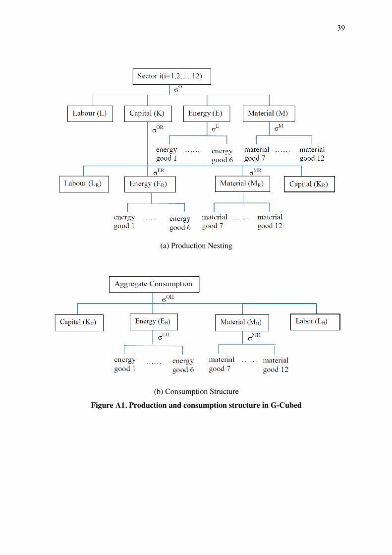
39

(a) Production Nesting

(b) Consumption Structure

Figure A1. Production and consumption structure in G-Cubed