engr 151: materials of engineering midterm 1 review material · 2017-03-02 · midterm 1 general...
TRANSCRIPT

MIDTERM 1 REVIEW MATERIAL
ENGR 151: Materials of Engineering

MIDTERM 1
General properties of materials
Bonding (primary, secondary and sub-types)
Properties of different kinds of bonds
Types of materials (metals, non-metals, ceramics,
polymers, semiconductors) and their characteristics
Different cell structures and properties (APF,
coordination number, relationship between a
and R, etc.)
Directions and planes
Geometric problems, sketching and interpreting
MIDTERM 1
Different coordinate systems (e.g. Miller-
Bravais)
Conversion from one system to the other
Density calculations (linear, planar)
Bragg’s law problems
Read Chapter 1 from textbook

CHAPTER 1 - INTRODUCTION
Metals used in structures & machinery
Plastics used in packaging, medical devices, consumer goods, clothing
Ceramics used in electronics (insulative)
Composites are novel materials for all applications listed above
4

CHAPTER 2 OBJECTIVES
Understand the elements used to make engineering materials
Review basic chemistry and physics principles
Overview of the materials classes:
Metals: good conductors, strong, lustrous
Polymers: organic, low densities, flexible
Ceramics: clay, cement, glass; insulators
Composites: fiberglass; strength and flexibility
5

ATOMIC STRUCTURE
Elements
Atomic number (Z, number of protons in nucleus)
Protons, neutrons, electrons (masses)
mp = mn = 1.67 x 10⁻²⁷ kg, me = 9.11 x 10⁻³¹ kg
Atomic Mass (A) = sum of proton and neutron masses in nucleus
Isotope = same element, differing atomic masses E.g. Hydrogen (P = 1, N = 0), Deuterium (P = 1, N = 1), Tritium (P
= 1, N = 2).
Atomic Weight = Average atomic mass of all naturally-occurring isotopes.
amu (atomic mass unit) = 1/12 of atomic mass of carbon 12
One mole = 6.023 x 10²³ (Avogadro’s number) atoms
6
ELECTRON CONFIGURATIONS
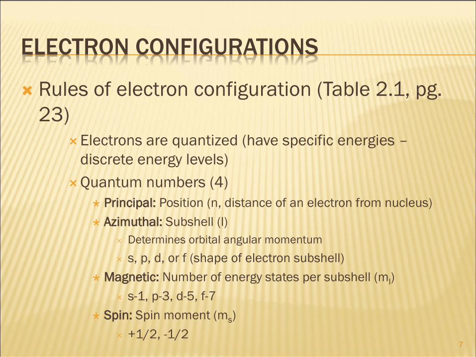
Rules of electron configuration (Table 2.1, pg.
23)
Electrons are quantized (have specific energies –
discrete energy levels)
Quantum numbers (4)
Principal: Position (n, distance of an electron from nucleus)
Azimuthal: Subshell (l)
Determines orbital angular momentum
s, p, d, or f (shape of electron subshell)
Magnetic: Number of energy states per subshell (ml)
s-1, p-3, d-5, f-7
Spin: Spin moment (ms)
+1/2, -1/2
7

ELECTRON CONFIGURATIONS – CONTD.
8
ELECTRON CONFIGURATIONS – CONTD.
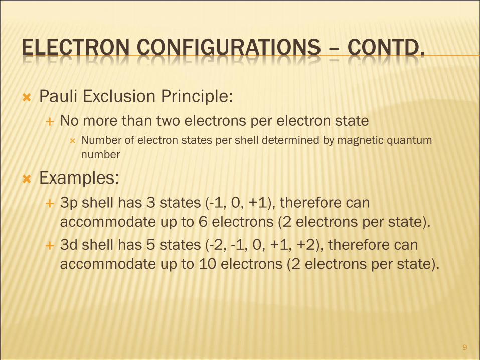
Pauli Exclusion Principle:
No more than two electrons per electron state
Number of electron states per shell determined by magnetic quantum
number
Examples:
3p shell has 3 states (-1, 0, +1), therefore can
accommodate up to 6 electrons (2 electrons per state).
3d shell has 5 states (-2, -1, 0, +1, +2), therefore can
accommodate up to 10 electrons (2 electrons per state).
9

QUICK REVIEW (TABLE 2.2, PG. 22)
How many valence electrons do they have?
Hydrogen, 1s1
Aluminum, 1s22s22p63s23p1
Chlorine, 1s22s22p63s23p5
Answer: 1, 3, 7
10
ELECTRONEGATIVITY
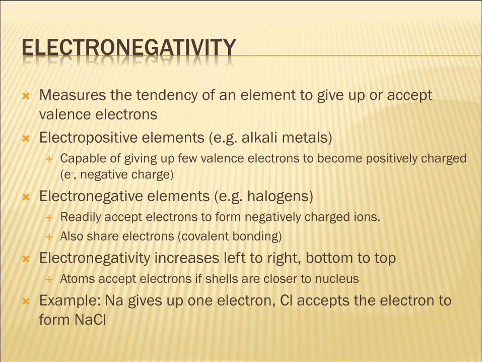
Measures the tendency of an element to give up or accept
valence electrons
Electropositive elements (e.g. alkali metals)
Capable of giving up few valence electrons to become positively charged
(e-, negative charge)
Electronegative elements (e.g. halogens)
Readily accept electrons to form negatively charged ions.
Also share electrons (covalent bonding)
Electronegativity increases left to right, bottom to top
Atoms accept electrons if shells are closer to nucleus
Example: Na gives up one electron, Cl accepts the electron to
form NaCl

ATOMIC BONDING
To understand the physical properties behind
materials, we must have an understanding of
interatomic forces that bind atoms together.
At large distances, the interactions between
two atoms are negligible…BUT…as they come
closer to each other they start to exert a force
on each other.

ATOMIC BONDING
There are two types of forces that are both
functions of the distance between two atoms:
1) Attractive Force (FA) – Depends on
bonding between atoms
2) Repulsive Force (FR) – Originates due
to repulsion between atoms’ individual
(negatively-charged) electron clouds

ATOMIC BONDING
Magnitude of an attractive force varies with
distance.
The Net Force (FN) is the sum of the attractive
and repulsive forces:
ATOMIC BONDING – CONTD.
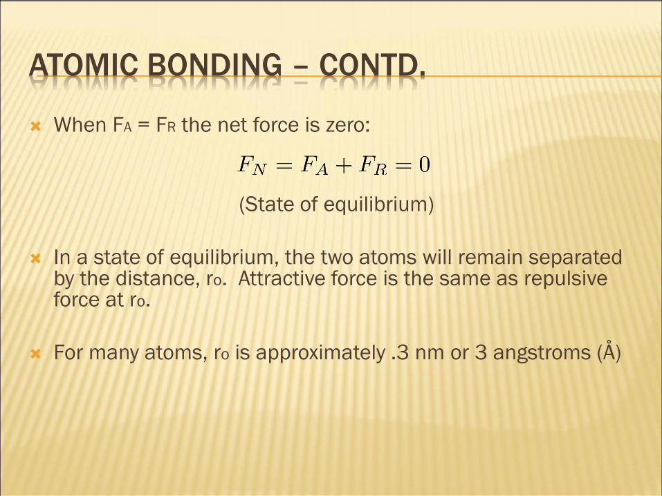
When FA = FR the net force is zero:
(State of equilibrium)
In a state of equilibrium, the two atoms will remain separated by the distance, ro. Attractive force is the same as repulsive force at ro.
For many atoms, ro is approximately .3 nm or 3 angstroms (Å)

ATOMIC BONDING – CONTD.
Another way to represent this relationship in attractive and repulsive forces is to look at potential energy relationships.
Force-energy relationships: Both force and energy are functions of distance r
Measure of amount of work done to move an atom from infinity (zero force) to a distance r.
Alternatively:

ATOMIC BONDING – CONTD.
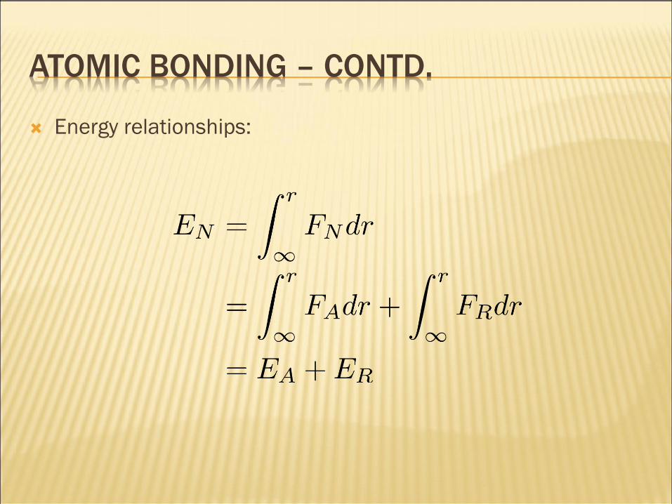
Energy relationships:
EN = net energy
EA = attractive energy
ER = repulsive energy
ATOMIC BONDING – CONTD.
Energy relationships:

Why does zero force correspond to minimum energy?
ATOMIC BONDING – CONTD.
The net potential energy curve has a trough
around its minimum. The potential energy
minimum is ro away from the origin.
Force is the derivative of energy.

ATOMIC BONDING – CONTD.
The Bonding Energy, Eo, refers to the vertical
distance between the minimum potential
energy and the x-axis. This is the energy that
would be required to separate the atoms to an
infinite separation.
Force and Energy plots become more complex
in actual materials. Why?

ATOMIC BONDING ENERGY
Magnitude of bonding energy and shape of
energy-versus-interatomic separation curve
vary from material to material AND depend on
the type of bonding that is taking place
between atoms.
ATOMIC BONDING ENERGY (EO)
Materials with large Bonding Energies also have high MELTING POINTS
At room temperature, materials with high bonding energy are in the SOLID STATE; those with small bonding energy are in the GASEOUS STATE; LIQUID STATE for intermediate bonding energy
FLEXIBILITY: stiff materials have a steep slope at the r=ro position; the slope is less steep for more flexible materials. Flexibility or hardness of a material is gauged by the MODULUS of ELASTICITY.
How much a material expands upon heating or contracts upon cooling is related to the potential energy curve. This is called LINEAR COEFFICIENT of THERMAL EXPANSION.
TYPES OF ATOMIC BONDING
Three types of PRIMARY bonds: IONIC,
COVALENT, METALLIC.
Nature of the bond depends on the electron
structures of the bonding atoms AND type of
bond depends on the tendency of atoms to
assume stable electron structures (completely
filling outermost electron shell)

IONIC BONDING
Always found in compounds that are formed by reactions between metallic and nonmetallic elements (elements at the horizontal extremities of the periodic table).
Metallic elements easily give up valence electrons to nonmetallic atoms.
In this process, all atoms acquire stable or inert gas configurations and electrical charges (becoming ions)

IONIC BONDING
The attractive bonding forces within ionic bonds are
COULOMBIC (positive and negative ions attracting one
another).
E.g. Na + Cl Na+ + Cl- NaCl
Notice the crystalline structure in the diagrams below.
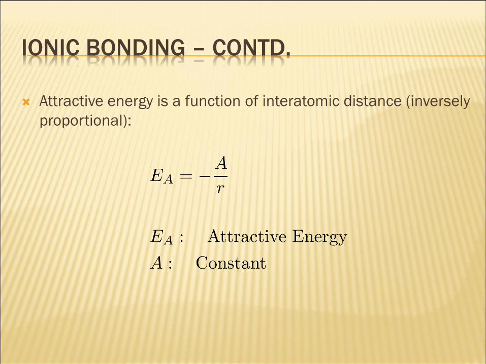
IONIC BONDING – CONTD.
Attractive energy is a function of interatomic distance (inversely
proportional):

IONIC BONDING – CONTD.
Constant A is expressed as:
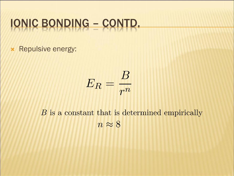
IONIC BONDING – CONTD.
Repulsive energy:

IONIC BONDING – CONTD.
Equation for attractive force:

COVALENT BONDING
Stable electron configurations are assumed by
the sharing of electrons between adjacent
atoms.
Atoms contribute at least one electron to the
bond, and the shared electrons are considered
to belong to both atoms
Covalent bonds are directional (between
specific atoms)
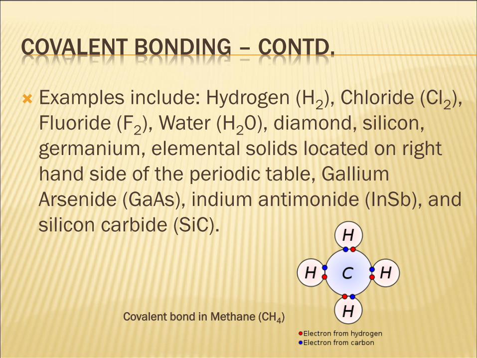
COVALENT BONDING – CONTD.
Examples include: Hydrogen (H2), Chloride (Cl2),
Fluoride (F2), Water (H20), diamond, silicon,
germanium, elemental solids located on right
hand side of the periodic table, Gallium
Arsenide (GaAs), indium antimonide (InSb), and
silicon carbide (SiC).
Covalent bond in Methane (CH4)
COVALENT BONDING
The number of covalent bonds for an atom is
determined by the number of valence
electrons.
For N' valence electrons, an atom can
covalently bond with at most 8 - N' other atoms.

METALLIC BONDING
Metallic materials have one, two, or at most three valence
electrons which are not bound to any atom within the solid and
can drift throughout the metal
Creates a “sea of electrons” (electrons that belong to the entire
metal)
Remaining nonvalence electrons and their atomic nuclei are
called ION CORES (have net positive charge equal in magnitude
to total valence charge per atom)

METALLIC BONDING – CONTD.
Free electrons shield ion cores from repulsive forces
and act as glue to hold ion cores together
Metallic bond is nondirectional
Free electrons allow metal to be good conductors of
heat and electricity
METALLIC BONDING ENERGIES
Can be strong or weak (Mercury, 68 kJ/mol, -
39 degrees Celsius; Tungsten, 850 kJ/mol,
3410 degrees Celsius)

SECONDARY BONDING
Very weak bonds (10 kJ/mol)
Exist between all atoms and molecules but obscured if other primary bonding is occurring
Found in:
inert gases because of their stable electron structures
between molecules that are covalently bonded
arise from dipoles (separation of positive and negative portions of an atom or molecule).
Also known as van der Waals bonding or physical bonding.
Physical, as opposed to chemical bonding – weaker bonds.

SECONDARY BONDING – CONTD.
+ -
+ -
Atomic or Molecular Dipoles
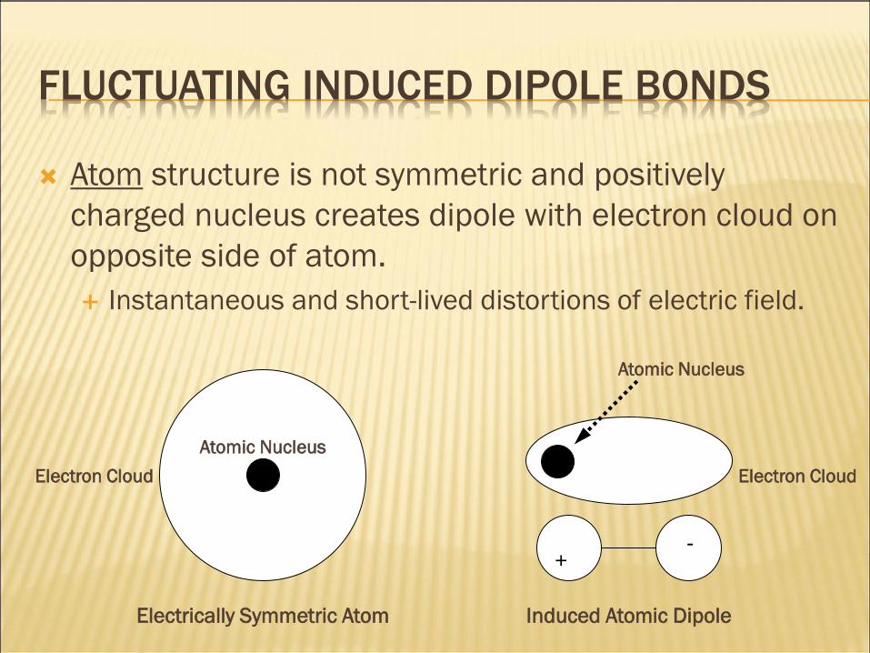
FLUCTUATING INDUCED DIPOLE BONDS
Atom structure is not symmetric and positively
charged nucleus creates dipole with electron cloud on
opposite side of atom.
Instantaneous and short-lived distortions of electric field.
+ -
Electrically Symmetric Atom
Induced Atomic Dipole
Atomic Nucleus
Electron Cloud
Atomic Nucleus
Electron Cloud
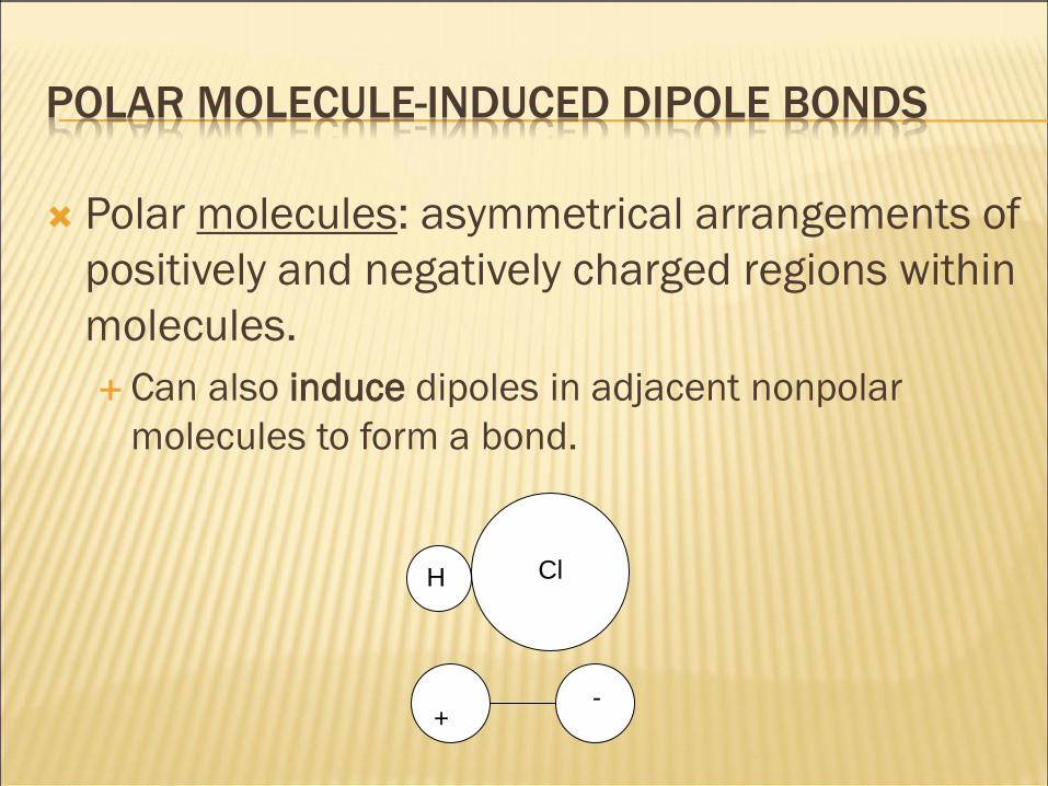
POLAR MOLECULE-INDUCED DIPOLE BONDS
Polar molecules: asymmetrical arrangements of
positively and negatively charged regions within
molecules.
Can also induce dipoles in adjacent nonpolar
molecules to form a bond.
H
Cl
+ -
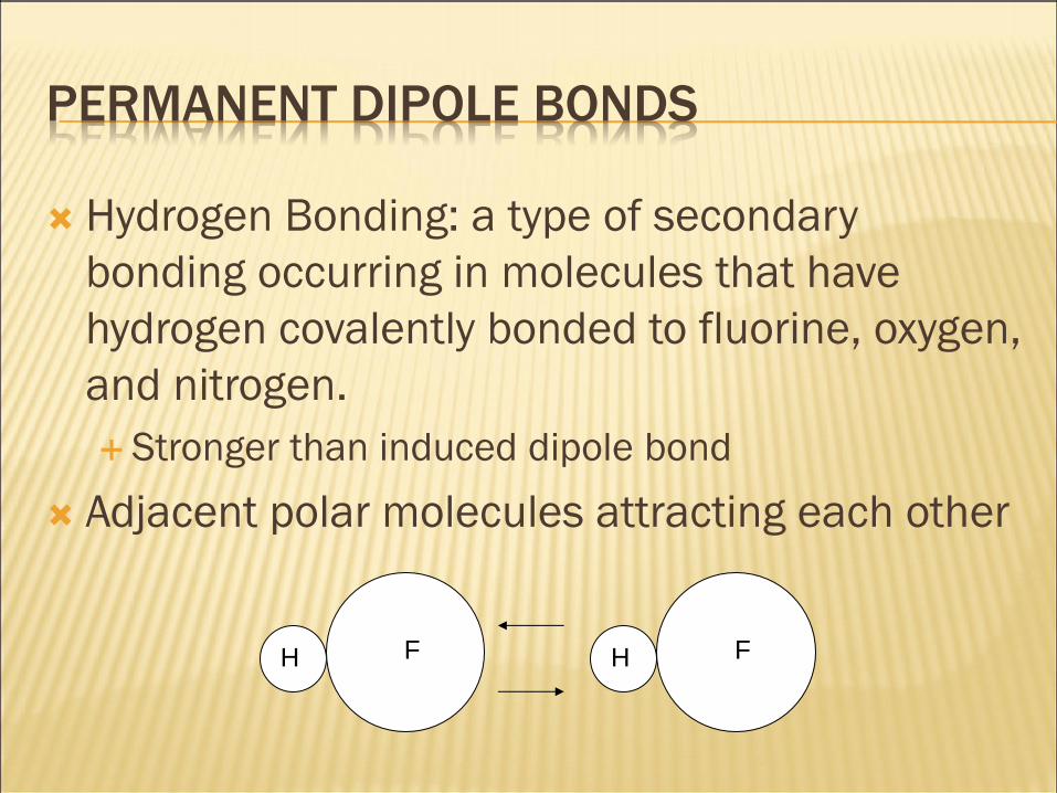
PERMANENT DIPOLE BONDS
Hydrogen Bonding: a type of secondary
bonding occurring in molecules that have
hydrogen covalently bonded to fluorine, oxygen,
and nitrogen.
Stronger than induced dipole bond
Adjacent polar molecules attracting each other
H
F H
F

SUMMARY OF BONDING TYPES
Bonding
Primary
Secondary
Ionic
Covalent
Metallic
Fluctuating Induced
Dipole Bonds
Polar Molecule-Induced
Dipole Bonds
Permanent Dipole
Bonds
CRYSTAL STRUCTURE
Material properties depend on crystal structure of the material
Atoms are thought of as being solid spheres having well-defined diameters (atomic hard sphere model, atoms touching each other)
Lattice: three-dimensional array of points coinciding with atom positions (sphere centers)
43

CRYSTAL STRUCTURE – CONTD.
44

UNIT CELLS
Subdivide the crystal structure into small
repeating entities called UNIT CELLS
These cells are mainly in cubes, prisms, six-
sided figures – regular, repeating geometric
structures
Geometric symmetry
The unit cell is the basic structural unit or
building block of crystal structure
45

METALLIC CRYSTAL STRUCTURES
No restrictions as to the number and position
of nearest-neighbor atoms (dense atomic
packing)
Each sphere in atomic hard sphere model
equates to an ion core
46
METALLIC CRYSTAL STRUCTURES CONTD.
Four simple crystal structures are found in
metals:
Simple Cubic (SC)
Face-Centered Cubic (FCC)
Body-Centered Cubic (BCC)
Hexagonal Close-Packed (HCP)
47
ANALYSIS TECNIQUES
Analysis of crystal structures gives insight into
properties of material such as strength, density,
how the material may behave under physicals
stress, etc.
Analysis steps:
Identify spatial geometries associated with unit cell
Relate dimensions of unit cell to atomic radius
Characterize/calculate required properties of
crystal structure
48
49
• Tend to be densely packed.
• Reasons for dense packing:
- Typically, only one element is present, so all atomic
radii are the same.
- Metallic bonding is not directional.
- Nearest neighbor distances tend to be small in
order to lower bond energy.
- Electron cloud shields cores from each other.
• Metals have the simplest crystal structures.
We will examine four such structures...
METALLIC CRYSTAL STRUCTURES
50
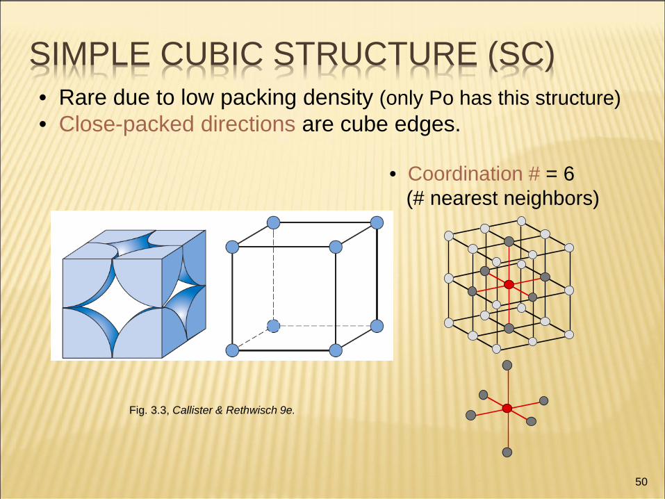
• Rare due to low packing density (only Po has this structure)
• Close-packed directions are cube edges.
• Coordination # = 6
(# nearest neighbors)
SIMPLE CUBIC STRUCTURE (SC)
Fig. 3.3, Callister & Rethwisch 9e.
51
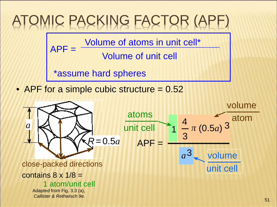
• APF for a simple cubic structure = 0.52
APF =
a 3
4
3 π (0.5a) 3 1
atoms
unit cell atom
volume
unit cell
volume
ATOMIC PACKING FACTOR (APF)
APF = Volume of atoms in unit cell*
Volume of unit cell
*assume hard spheres
Adapted from Fig. 3.3 (a),
Callister & Rethwisch 9e.
close-packed directions
a
R = 0.5a
contains 8 x 1/8 = 1 atom/unit cell
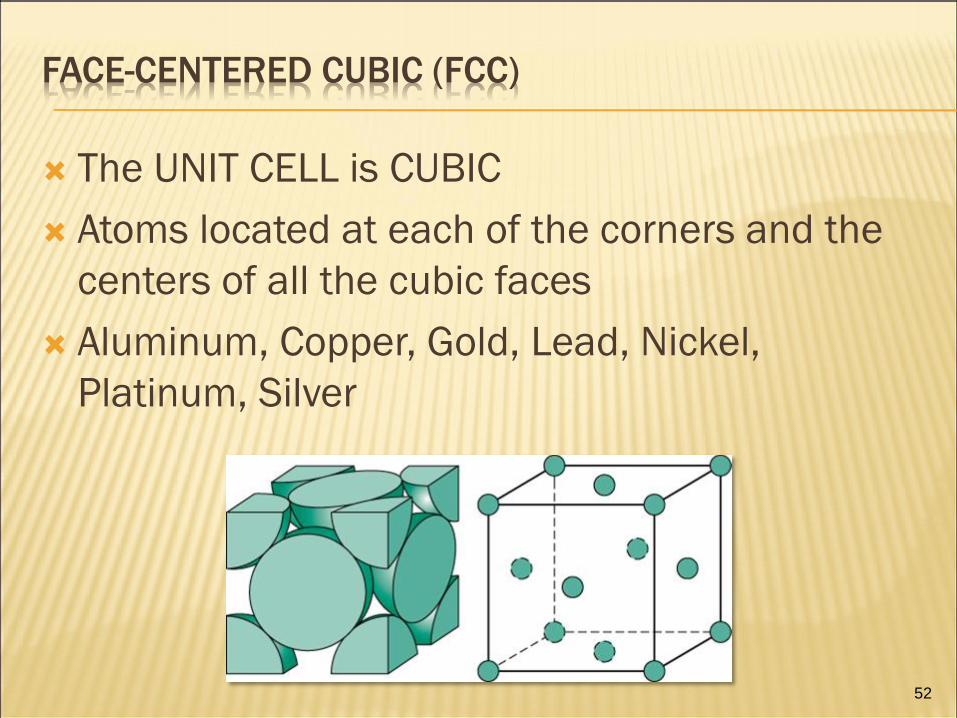
FACE-CENTERED CUBIC (FCC)
The UNIT CELL is CUBIC
Atoms located at each of the corners and the
centers of all the cubic faces
Aluminum, Copper, Gold, Lead, Nickel,
Platinum, Silver
52
FACE-CENTERED CUBIC
The cube edge length a and the atomic radius
are related through:
a = 2R√2
53
54
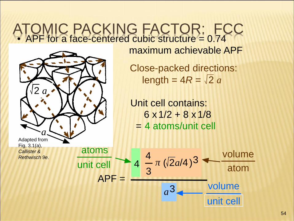
• APF for a face-centered cubic structure = 0.74 ATOMIC PACKING FACTOR: FCC
maximum achievable APF
APF =
4
3 π ( 2 a/4 ) 3 4
atoms
unit cell atom
volume
a 3
unit cell
volume
Close-packed directions:
length = 4R = 2 a
Unit cell contains: 6 x 1/2 + 8 x 1/8 = 4 atoms/unit cell
a
2 a
Adapted from
Fig. 3.1(a),
Callister &
Rethwisch 9e.

FCC
Each corner atom is shared by eight unit cells
(Eight 1/8 portions per unit cell)
Each face atom is shared by two unit cells (six
½ portions per unit cell)
Grand total of four whole atoms per unit cell
55
COORDINATION NUMBER
The number of nearest neighbor or touching
atoms
The coordination number for FCC is ??
56

COORDINATION NUMBER
The number of nearest neighbor or touching
atoms
The coordination number for FCC is 12
57
ATOMIC PACKING FACTOR (APF)
The fraction of solid sphere volume in a unit
cell:
Volume of atoms in a unit cell
Total unit cell volume
Using the APF equation and the volume of an
FCC unit cell, find the APF of a FCC crystal
structure
APF =
58
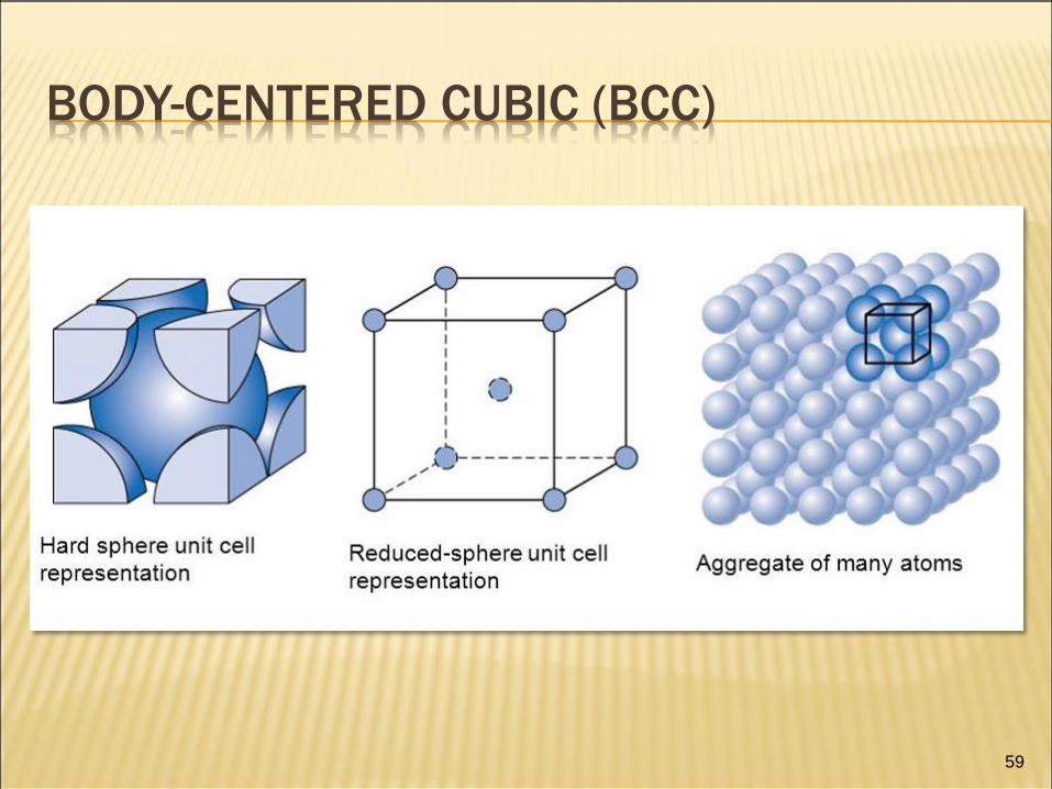
BODY-CENTERED CUBIC (BCC)
59

BCC
Atoms located in all eight corners and a single
atom at the cube center
Derive an expression for the unit cell edge
length (a) using the atomic radius (R)
60
61
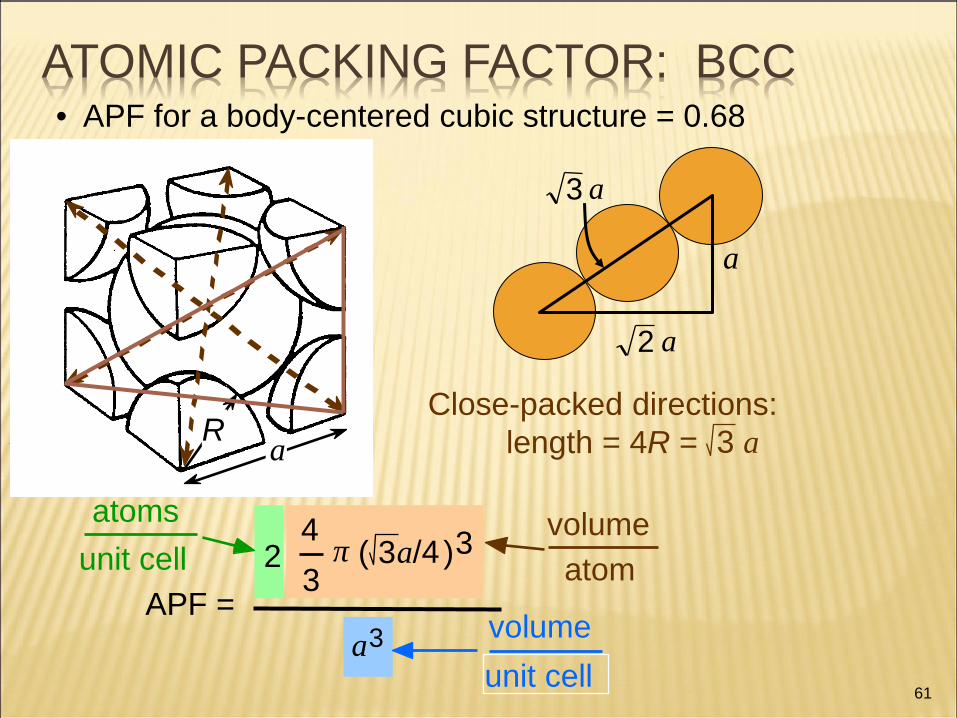
ATOMIC PACKING FACTOR: BCC
APF =
4
3 π ( 3 a/4 ) 3 2
atoms
unit cell atom
volume
a 3
unit cell
volume
length = 4R =
Close-packed directions:
3 a
• APF for a body-centered cubic structure = 0.68
Adapted from
Fig. 3.2(a), Callister &
Rethwisch 9e.
a
a 2
a 3
a R
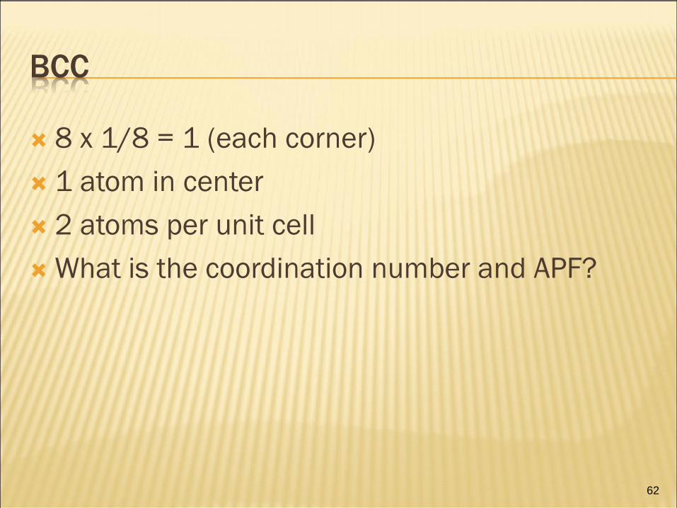
BCC
8 x 1/8 = 1 (each corner)
1 atom in center
2 atoms per unit cell
What is the coordination number and APF?
62
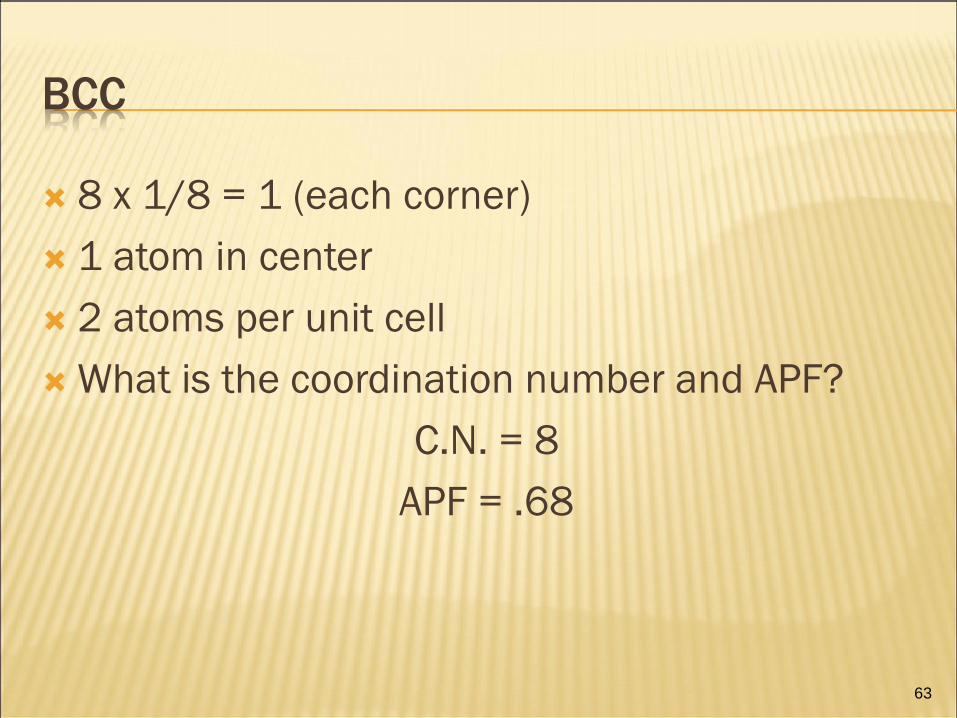
BCC
8 x 1/8 = 1 (each corner)
1 atom in center
2 atoms per unit cell
What is the coordination number and APF?
C.N. = 8
APF = .68
63

HEXAGONAL CLOSE-PACKED (HCP)
Unit cell is hexagonal
Six atoms form a regular hexagon and surround
a single atom
Another plane is situated in between top and
bottom plane (provides three additional atoms)
64

HCP
Six atoms altogether within unit cell
65

HCP
Six atoms altogether within unit cell
1/6 x 12 (top and bottom plane portions
½ x 2 (center face atoms)
3 midplane interior atoms
C.N. = 12
APF = .74
c/a = 1.633
66

OVERVIEW
Crystal
Structure
Relationship
between a
and R (cubic
structures)
Number of
atoms per
unit cell
Coordination
Number APF
FCC 4 12 0.74
BCC 2 8 0.68
HCP ------ 6 12 0.74
67
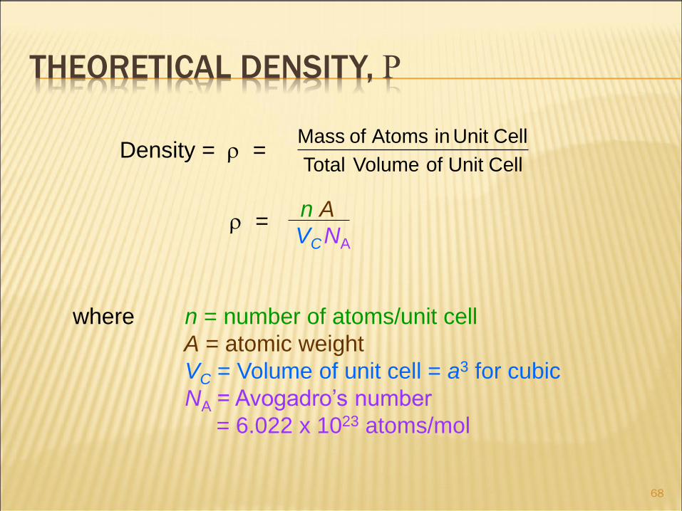
THEORETICAL DENSITY, R
68
where n = number of atoms/unit cell
A = atomic weight
VC = Volume of unit cell = a3 for cubic
NA = Avogadro’s number
= 6.022 x 10²³ atoms/mol
Density = =
VC NA
n A =
Cell Unit of Volume Total
Cell Unit in Atoms of Mass

THEORETICAL DENSITY, R
Ex: Cr (BCC)
A (atomic weight) = 52.00 g/mol
n = 2 atoms/unit cell
R = 0.125 nm
69
theoretical
a = 4R/ 3 = 0.2887 nm
actual
a R
= a 3
52.00 2
atoms
unit cell mol
g
unit cell
volume atoms
mol
6.022 x 1023
= 7.18 g/cm3
= 7.19 g/cm3

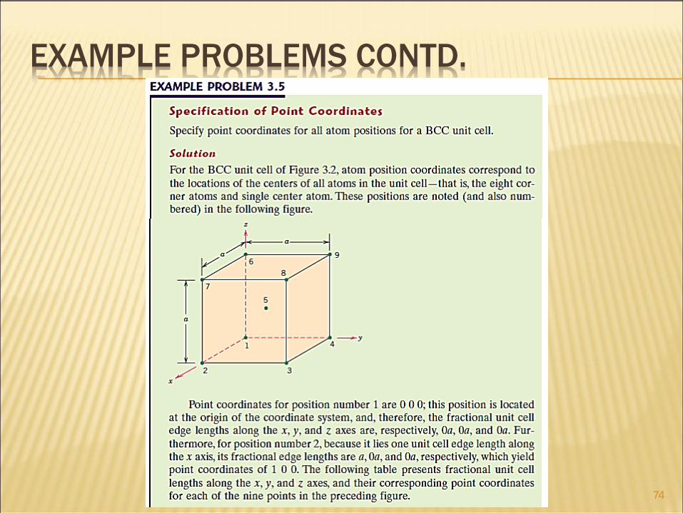
• Coordinates of selected points in the unit cell.
• The number refers to the distance from the origin in terms
of lattice parameters.
Point Coordinates
• Each unit cell is a reference or basis.
• The length of an edge is normalized as a unit of
measurement.
• E.g. if the length of the edge of the unit cell along the
X-axis is a, then ALL measurements in the X-direction
are referenced to a (e.g. a/2).
Point Coordinates – Contd.
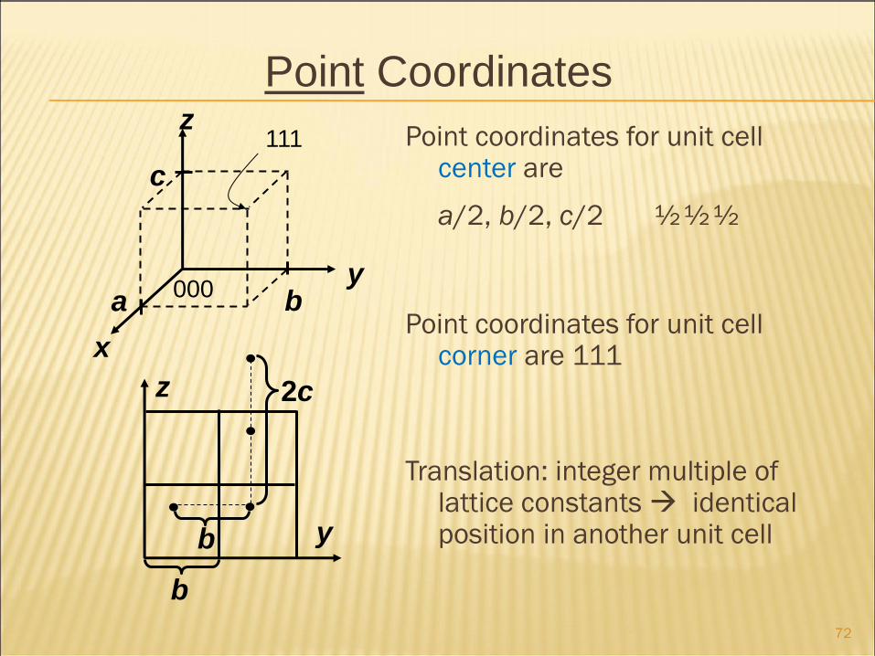
Point coordinates for unit cell center are
a/2, b/2, c/2 ½ ½ ½
Point coordinates for unit cell corner are 111
Translation: integer multiple of lattice constants identical position in another unit cell
72
z
x
y a b
c
000
111
y
z
2c
b
b
Point Coordinates
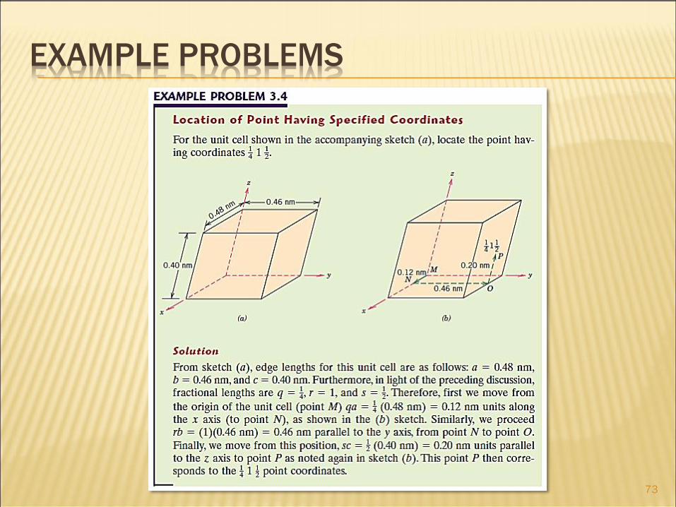
EXAMPLE PROBLEMS
73
EXAMPLE PROBLEMS CONTD.
74

EXAMPLE PROBLEMS CONTD.
75

Determine the Miller indices of directions A, B, and C.
Miller Indices, Directions
(c) 2003 Brooks/Cole Publishing /
Thomson Learning™

GENERAL APPROACH FOR MILLER INDICES
77
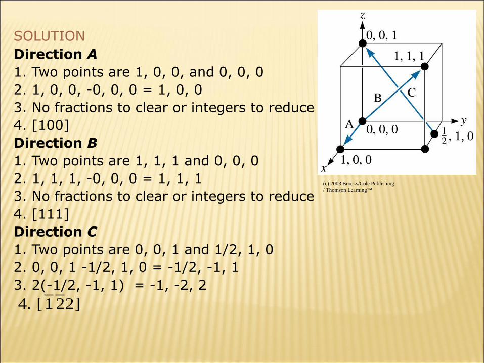
SOLUTION
Direction A
1. Two points are 1, 0, 0, and 0, 0, 0
2. 1, 0, 0, -0, 0, 0 = 1, 0, 0
3. No fractions to clear or integers to reduce
4. [100]
Direction B
1. Two points are 1, 1, 1 and 0, 0, 0
2. 1, 1, 1, -0, 0, 0 = 1, 1, 1
3. No fractions to clear or integers to reduce
4. [111]
Direction C
1. Two points are 0, 0, 1 and 1/2, 1, 0
2. 0, 0, 1 -1/2, 1, 0 = -1/2, -1, 1
3. 2(-1/2, -1, 1) = -1, -2, 2
2]21[ .4
(c) 2003 Brooks/Cole Publishing
/ Thomson Learning™
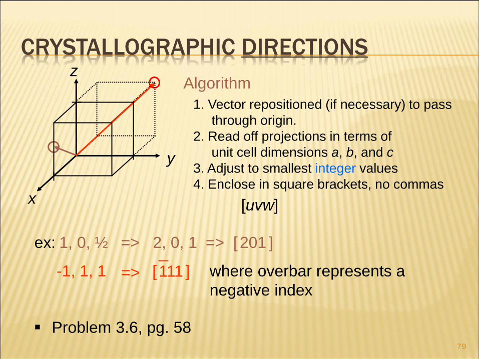
CRYSTALLOGRAPHIC DIRECTIONS
79
1. Vector repositioned (if necessary) to pass
through origin.
2. Read off projections in terms of
unit cell dimensions a, b, and c
3. Adjust to smallest integer values
4. Enclose in square brackets, no commas
[uvw]
ex: 1, 0, ½ => 2, 0, 1 => [ 201 ]
-1, 1, 1
z
x
Algorithm
where overbar represents a
negative index
[ 111 ] =>
y
Problem 3.6, pg. 58

EXAMPLE PROBLEMS
80
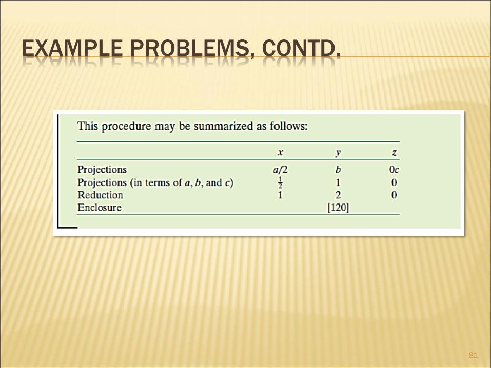
EXAMPLE PROBLEMS, CONTD.
81

EXAMPLE PROBLEMS, CONTD.
82
Exam problems – make
sure you translate and
scale vector to fit WITHIN
unit cube if asked!
83
HCP CRYSTALLOGRAPHIC DIRECTIONS
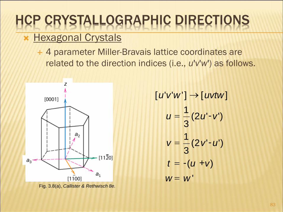
Hexagonal Crystals
4 parameter Miller-Bravais lattice coordinates are
related to the direction indices (i.e., u'v'w') as follows.
=
=
=
' w w
t
v
u
) v u ( + -
) ' u ' v 2 ( 3
1 -
) ' v ' u 2 ( 3
1 - =
] uvtw [ ] ' w ' v ' u [
Fig. 3.8(a), Callister & Rethwisch 8e.
- a3
a1
a2
z

84
HCP CRYSTALLOGRAPHIC DIRECTIONS
Fig. 3.8(a), Callister & Rethwisch 8e.
- a3
a1
a2
z
85
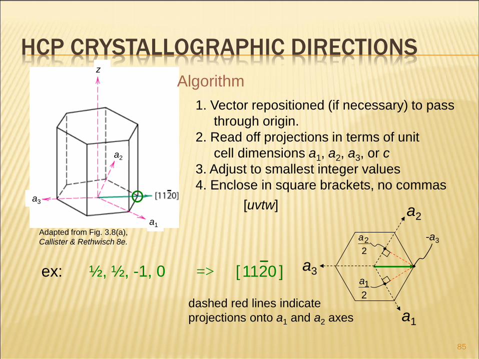
HCP CRYSTALLOGRAPHIC DIRECTIONS
1. Vector repositioned (if necessary) to pass
through origin.
2. Read off projections in terms of unit
cell dimensions a1, a2, a3, or c
3. Adjust to smallest integer values
4. Enclose in square brackets, no commas
[uvtw]
[ 1120 ] ex: ½, ½, -1, 0 =>
Adapted from Fig. 3.8(a),
Callister & Rethwisch 8e.
dashed red lines indicate
projections onto a1 and a2 axes a1
a2
a3
-a3
2
a 2
2
a 1
- a3
a1
a2
z
Algorithm
86
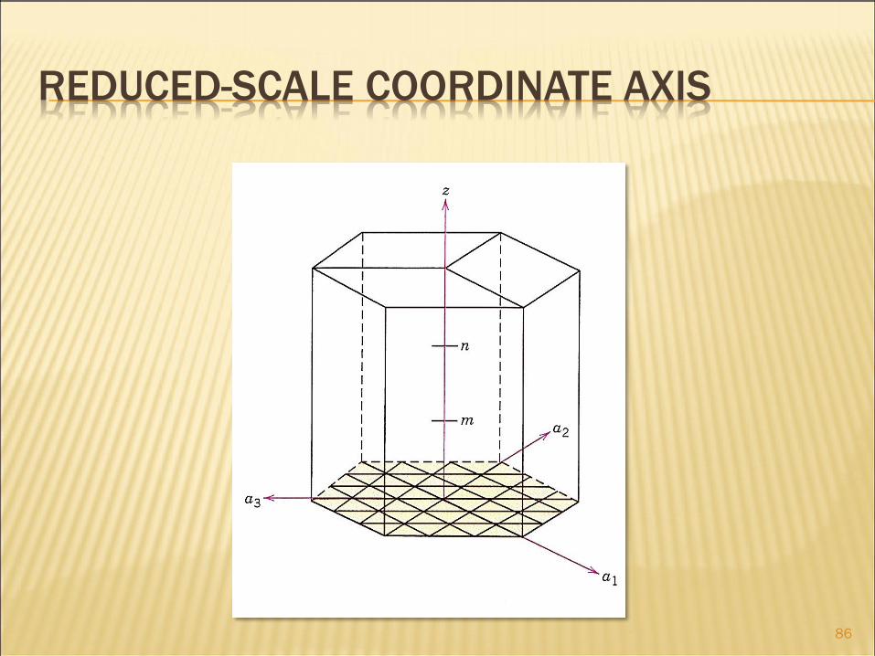
REDUCED-SCALE COORDINATE AXIS

87
PROBLEM 3.8

88
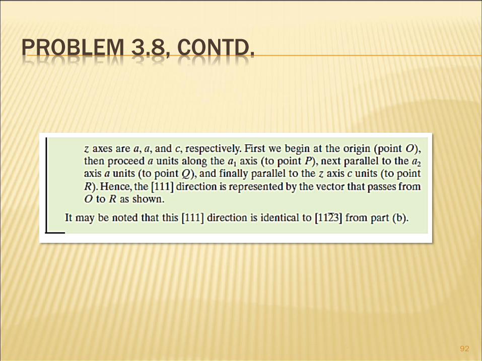
PROBLEM 3.8, CONTD.

89
PROBLEM 3.8, CONTD.

90
PROBLEM 3.8, CONTD.

91
PROBLEM 3.8, CONTD.
92
PROBLEM 3.8, CONTD.
93
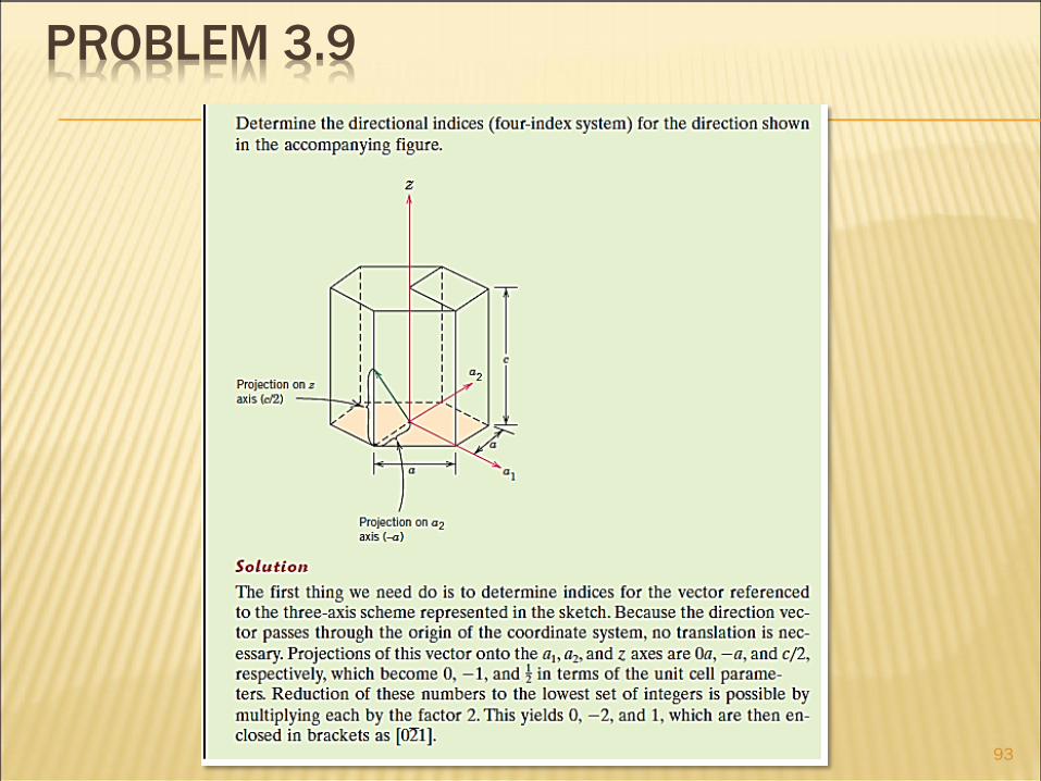
PROBLEM 3.9
94
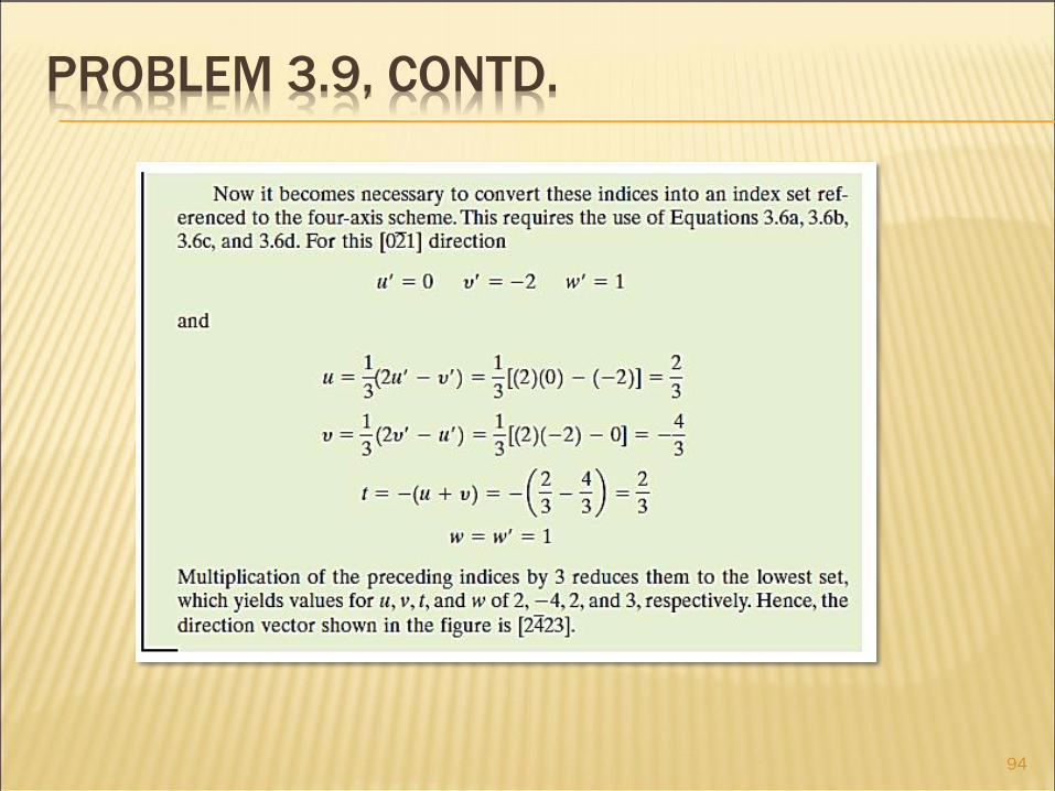
PROBLEM 3.9, CONTD.
95
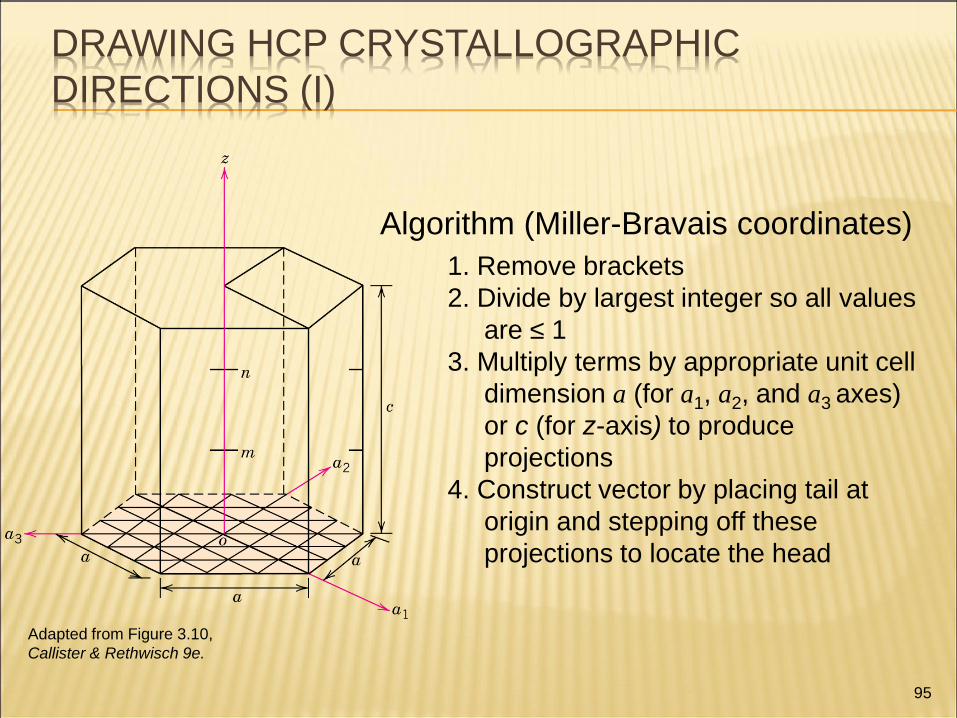
DRAWING HCP CRYSTALLOGRAPHIC
DIRECTIONS (I)
1. Remove brackets
2. Divide by largest integer so all values
are ≤ 1
3. Multiply terms by appropriate unit cell
dimension a (for a1, a2, and a3 axes)
or c (for z-axis) to produce
projections
4. Construct vector by placing tail at
origin and stepping off these
projections to locate the head
Algorithm (Miller-Bravais coordinates)
Adapted from Figure 3.10,
Callister & Rethwisch 9e.

96
DRAWING HCP CRYSTALLOGRAPHIC
DIRECTIONS (II)
Draw the direction in a hexagonal unit cell.
[1213]
4. Construct Vector
1. Remove brackets -1 -2 1 3
Algorithm a1 a2 a3 z
2. Divide by 3 1 3
1
3
2
3
1
3. Projections
proceed –a/3 units along a1 axis to point p
–2a/3 units parallel to a2 axis to point q
a/3 units parallel to a3 axis to point r
c units parallel to z axis to point s
[1 2 13]
p
q r
s
start at point o
Adapted from p. 72,
Callister &
Rethwisch 9e.
[1213] direction represented by vector from point o to point s
97
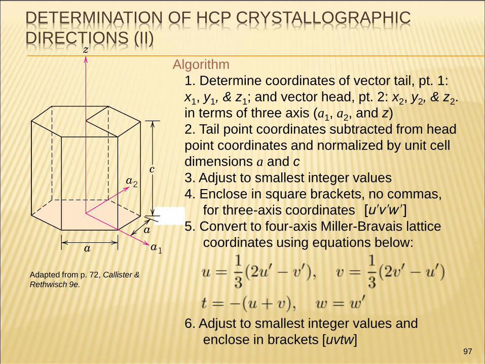
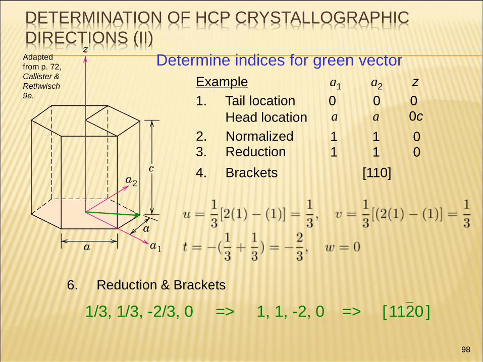
1. Determine coordinates of vector tail, pt. 1:
x1, y1, & z1; and vector head, pt. 2: x2, y2, & z2.
in terms of three axis (a1, a2, and z)
2. Tail point coordinates subtracted from head
point coordinates and normalized by unit cell
dimensions a and c
3. Adjust to smallest integer values
4. Enclose in square brackets, no commas,
for three-axis coordinates
5. Convert to four-axis Miller-Bravais lattice
coordinates using equations below:
6. Adjust to smallest integer values and
enclose in brackets [uvtw]
Adapted from p. 72, Callister &
Rethwisch 9e.
Algorithm
DETERMINATION OF HCP CRYSTALLOGRAPHIC
DIRECTIONS (II)
98
4. Brackets [110]
1. Tail location 0 0 0
Head location a a 0c
1 1 0 3. Reduction 1 1 0
Example a1 a2 z
1/3, 1/3, -2/3, 0 => 1, 1, -2, 0 => [ 1120 ]
6. Reduction & Brackets
Adapted
from p. 72,
Callister &
Rethwisch
9e.
DETERMINATION OF HCP CRYSTALLOGRAPHIC
DIRECTIONS (II)
Determine indices for green vector
2. Normalized

FAMILIES OF DIRECTIONS <UVW>
For some crystal structures, several
nonparallel directions with different
indices are crystallographically equivalent;
this means that atom spacing along each
direction is the same.
99
100
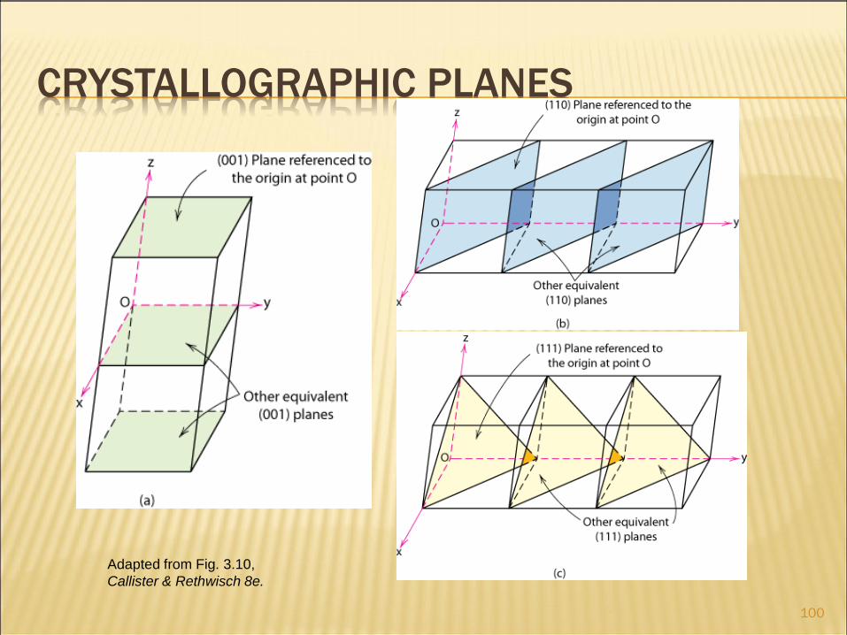
CRYSTALLOGRAPHIC PLANES
Adapted from Fig. 3.10,
Callister & Rethwisch 8e.

101
CRYSTALLOGRAPHIC PLANES
Miller Indices: Reciprocals of the (three) axial intercepts for a plane, cleared of fractions & common multiples. All parallel planes have same Miller indices.
Algorithm 1. Read off intercepts of plane with axes in terms of a, b, c 2. Take reciprocals of intercepts 3. Reduce to smallest integer values 4. Enclose in parentheses, no commas i.e., (hkl)

102
CRYSTALLOGRAPHIC PLANES z
x
y a b
c
4. Miller Indices (110)
example a b c z
x
y a b
c
4. Miller Indices (100)
1. Intercepts 1 1
2. Reciprocals 1/1 1/1 1/
1 1 0 3. Reduction 1 1 0
1. Intercepts 1/2
2. Reciprocals 1/½ 1/ 1/
2 0 0 3. Reduction 1 0 0
example a b c

103
CRYSTALLOGRAPHIC PLANES z
x
y a b
c
4. Miller Indices (634)
example 1. Intercepts 1/2 1 3/4
a b c
2. Reciprocals 1/½ 1/1 1/¾
2 1 4/3
3. Reduction 6 3 4
(001) (010),
Family of Planes {hkl}
(100), (010), (001), Ex: {100} = (100),

FAMILY OF PLANES
Planes that are crystallographically equivalent
have the same atomic packing.
Also, in cubic systems only, planes having the
same indices, regardless of order and sign,
are equivalent.
Ex: {111}
= (111), (111), (111), (111), (111), (111), (111), (111)
104
(001) (010), (100), (010), (001), Ex: {100} = (100),
_ _ _ _ _ _ _ _ _ _ _ _

FCC UNIT CELL WITH (110) PLANE
105

BCC UNIT CELL WITH (110) PLANE
106

107
CRYSTALLOGRAPHIC PLANES (HCP)
In hexagonal unit cells the same idea is used
example a1 a2 a3 c
4. Miller-Bravais Indices (1011) (hkil)
1. Intercepts 1 -1 1 2. Reciprocals 1 1/
1 0
-1
-1
1
1
3. Reduction 1 0 -1 1
a2
a3
a1
z
Adapted from Fig. 3.8(b),
Callister & Rethwisch 8e.
108
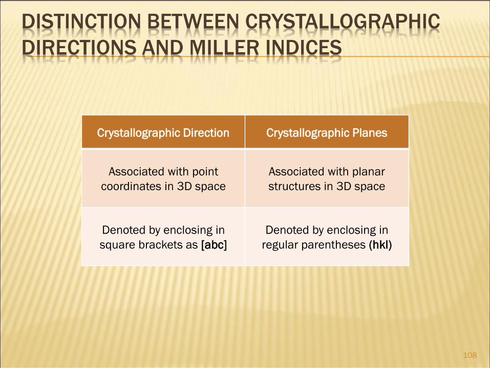
DISTINCTION BETWEEN CRYSTALLOGRAPHIC
DIRECTIONS AND MILLER INDICES
Crystallographic Direction Crystallographic Planes
Associated with point
coordinates in 3D space
Associated with planar
structures in 3D space
Denoted by enclosing in
square brackets as [abc]
Denoted by enclosing in
regular parentheses (hkl)

EXAMPLE PROBLEMS
109
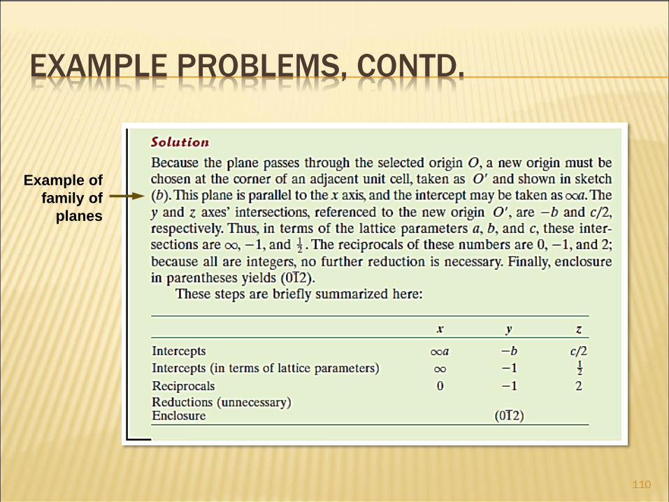
EXAMPLE PROBLEMS, CONTD.
110
Example of
family of
planes

EXAMPLE PROBLEMS, CONTD.
111
Don’t
forget to
slide plane
back within
unit cell!
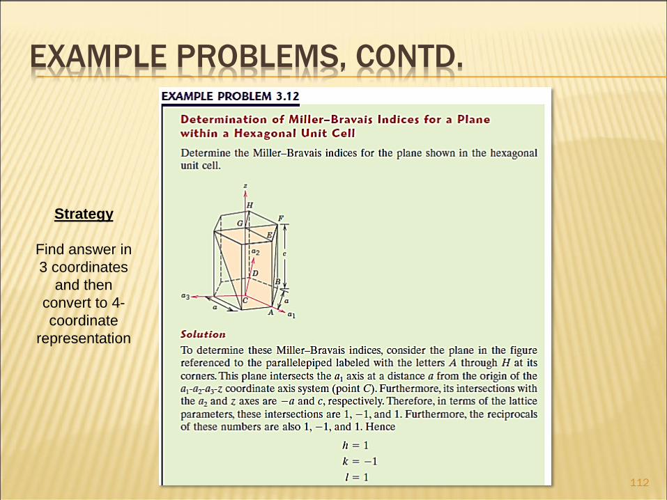
EXAMPLE PROBLEMS, CONTD.
112
Strategy
Find answer in
3 coordinates
and then
convert to 4-
coordinate
representation
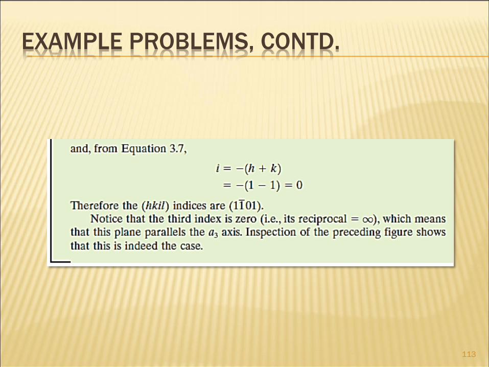
EXAMPLE PROBLEMS, CONTD.
113

114
ex: linear density of Al in [110]
direction
a = 0.405 nm
LINEAR DENSITY
Linear Density of Atoms LD =
a
[110]
Unit length of direction vector
Number of atoms
# atoms
length
3.5 atoms/nm a 2
2 LD = =
Adapted from Fig. 3.1(a),
Callister & Rethwisch 8e.
2 atoms per line, sharing computed
along vector length

115
PLANAR DENSITY OF (100) IRON Solution: At T < 912ºC iron has the BCC structure.
(100)
Radius of iron R = 0.1241 nm
R 3
3 4 a =
Adapted from Fig. 3.2(c), Callister & Rethwisch 8e.
2D repeat unit
= Planar Density = a 2
1
atoms
2D repeat unit
= nm2
atoms 12.1
m2
atoms = 1.2 x 10¹⁹
1
2
R 3
3 4 area
2D repeat unit
116
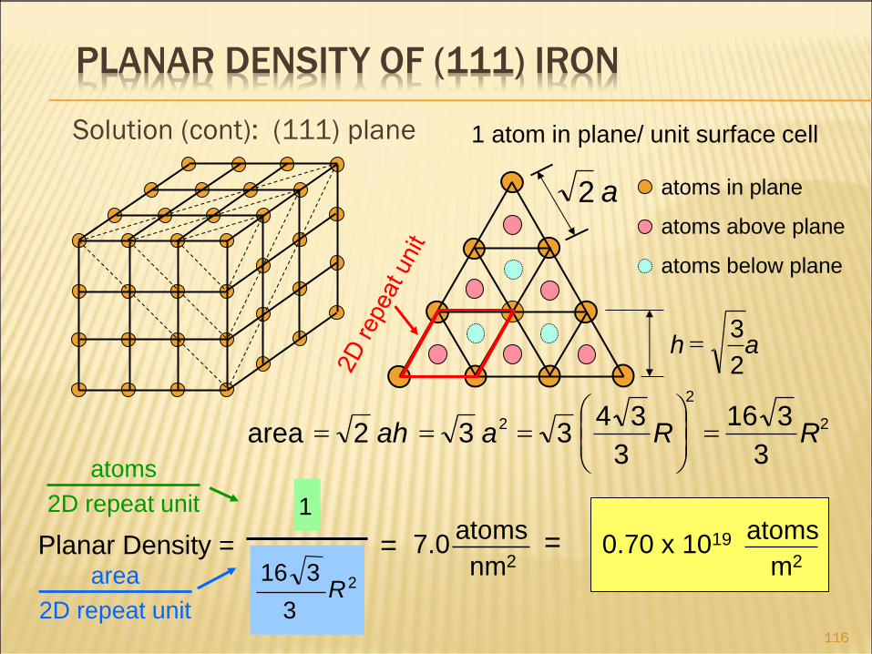
PLANAR DENSITY OF (111) IRON
Solution (cont): (111) plane 1 atom in plane/ unit surface cell
3 3 3
2
2
R 3
16 R
3
4
2 a 3 ah 2 area =
= = =
atoms in plane
atoms above plane
atoms below plane
a h 2
3 =
a 2
1
= = nm2
atoms 7.0
m2
atoms 0.70 x 10¹⁹
3 2 R 3
16 Planar Density =
atoms
2D repeat unit
area
2D repeat unit

CONSTRUCTIVE INTERFERENCE
Occurs at angle θ to the planes, if path length
difference is equal to a whole number, n, of
wavelengths (n equals order of reflection):
Bragg’s Law
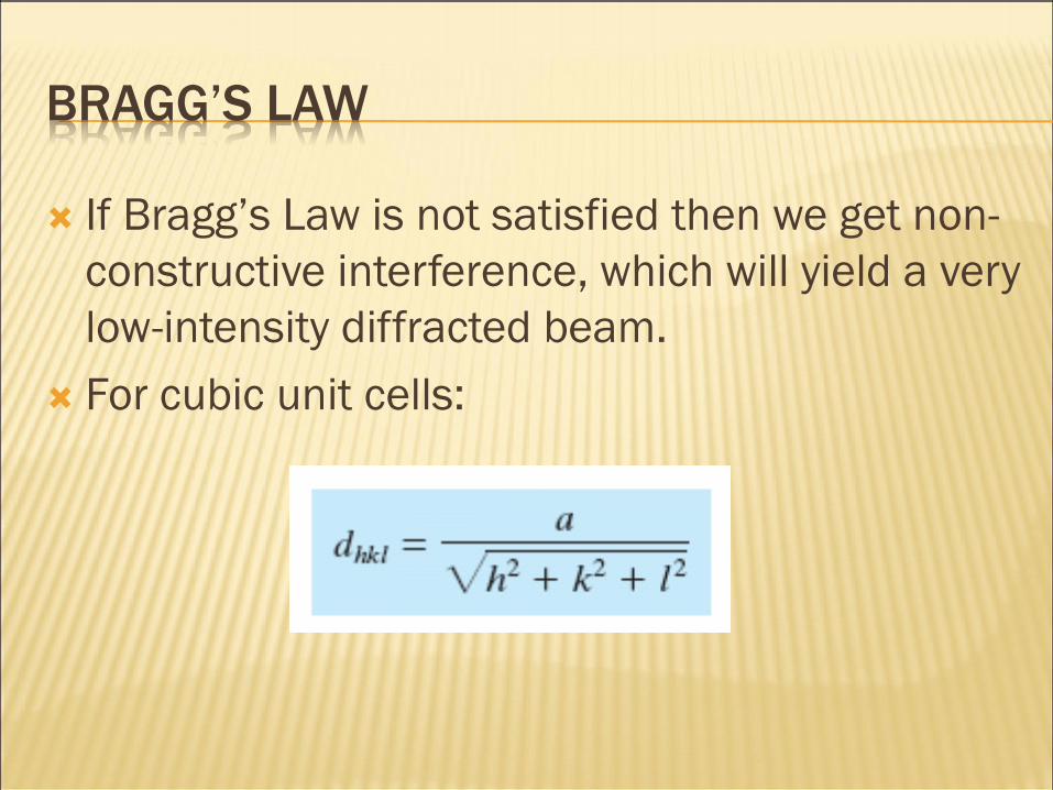
BRAGG’S LAW
If Bragg’s Law is not satisfied then we get non-
constructive interference, which will yield a very
low-intensity diffracted beam.
For cubic unit cells:

BRAGG’S LAW
Specifies when diffraction will occur for unit
cells having atoms positioned only at the cell
corners
Atoms at different locations act as extra
scattering centers and results in the absence of
some diffracted beams.

EXAMPLE PROBLEM
