Does Money Matter? The Effects of Cash Transfers on Child Health and Development in Rural Ecuador

by

Christina Paxson, Princeton University

Norbert Schady, World Bank

CEPS Working Paper No. 145 March 2007

Acknowledgements: We thank the Center for Economic Policy Studies at Princeton University, the Government of Ecuador, and the World Bank for funding for this study; Anne Case, Angus Deaton, Edward Miguel, and participants at seminars at Columbia University, Princeton University, and the American Economic Association 2007 Annual Meetings for their comments; and Tom Vogl and Lisa Vura-Weis for excellent research assistance. We also acknowledge the collaboration at every stage of this project with our colleagues at the Secretaría Técnica del Frente Social in Ecuador, in particular Santiago Izquierdo, Mauricio León, Ruth Lucio, Juan Ponce, José Rosero, and Yajaira Vázquez. This paper is a draft: Do not cite or quote without permission from the authors. Comments are welcome.

Does Money Matter? The Effects of Cash Transfers on Child Health and

Development in Rural Ecuador

March 2007

ABSTRACT

This paper examines how a government-run cash transfer program targeted to poor mothers in rural Ecuador influenced the health and development of their children. This program is of particular interest because, unlike other transfer programs that have been implemented recently in Latin America, receipt of the cash transfers was not conditioned on specific parental actions, such as taking children to health clinics or sending them to school. This feature of the program makes it possible to assess whether conditionality is necessary for programs to have beneficial effects on children. Random assignment at the parish level is used to identify the program’s effects. We find that the cash transfer program had positive effects on the physical, cognitive, and socio-emotional development of children, and the treatment effects were substantially larger for the poorer children than for less poor children. Among the poorest children in our sample, children whose mothers were eligible for transfers had outcomes that were on average more than 20 percent of a standard deviation higher than those for comparable children in the control group. Treatment effects are somewhat larger for girls and for children with more highly-educated mothers. We examine three mechanisms—better nutrition, greater use of health care, and better parenting—through which the transfers might influence child development. The program appeared to improve children’s nutrition and increased the chance they were treated for helminth infections. However, children in the treatment group were not more likely to visit health clinics for growth monitoring, and the mental health and parenting or their mothers did not improve. JEL codes: I12, O12 Christina Paxson Norbert Schady 316 Wallace Hall Development Research Group Princeton University Room MC 3-551 Princeton NJ 08544 World Bank cpaxson@princeton.edu Washington DC 20433 nschady@worldbank.org

I. Introduction

In 2003, the government of Ecuador launched a new cash transfer program—the Bono de

Desarrollo Humano (BDH)—targeted to poor families with children. The transfer is small—only

$15 per month per family—but it represents a non-trivial 10 percent increase in family

expenditure for the average eligible family. Unlike transfers made by a variety of programs in

Latin America, including the much-studied Oportunidades program in Mexico (formerly known

as PROGRESA), in Ecuador women in eligible families have received what is referred to as “the

Bono” with no strings attached.

Random assignment was built into the roll-out of the BDH. Two separate randomized

experiments were conducted. One was designed to examine the effects of the Bono on poverty

and educational attainment among school-aged children. The other experiment—which is the

concern of this paper—was designed to examine how the Bono affected the health and

development of pre-school aged children. Parishes were randomly assigned to “treatment” and

“control” groups. In treatment parishes, poor families with pre-school aged children were eligible

to receive the Bono early in the roll-out, in control parishes families were not offered the Bono

until several years later. The families under study were interviewed prior to the introduction of

the BDH, and again before the control parishes were included in the program.

The randomized introduction of the BDH provides an opportunity to answer a basic

question: how do cash transfers affect the health and development of young children? This

question is important because poor health and delayed development in early childhood may have

long-lasting consequences for health and economic status. Studies from developed countries that

have tracked children into adulthood show that healthier and taller children do better on tests of

cognitive ability; these children grow into taller adults, and earn significantly higher wages (Case

and Paxson 2006; see also Connolly, Micklewright, and Nickell, 1992; Currie and Thomas,

2

1999; Feinstein, 2003; Robertson and Symons, 2003). In poor countries, early childhood

developmental outcomes also appear to be important for success in early adulthood. A recent

review paper makes the case that early cognitive and socio-emotional development is a strong

predictor of school attainment in Guatemala, South Africa, the Philippines, Jamaica and Brazil,

even after controlling for wealth and maternal education (Grantham-McGregor et al., 2007). The

authors conclude that at least 200 million children in the developing world fail to reach their

potential in cognitive development, with serious consequences for their health as adults and for

their earnings capacity.

There is clear evidence that, within developing countries, children from lower income

families are more likely to experience worse health and to do less well on assessments of

cognitive and behavioral development. However, there is much less evidence on whether

improvements in income levels result in healthier children with better developmental outcomes.

The difficulty establishing causal effects of income on children’s outcomes is clear: while money

may improve children’s health and development, it could be that families that are better equipped

to earn higher incomes are also better able to produce and nurture healthier and more able

children. If so, income transfers may not have sizeable effects on child outcomes. It is also

possible that cross-sectional comparisons of children’s outcomes in families with more or less

income may understate the likely impact of cash transfers. Even with no strings attached,

recipients of cash from a social program may use it differently from other sources of income.

Women may also have different preferences from men, and cash transfers made to women may

have larger beneficial effects on children’s wellbeing than one would conclude from simple

comparisons of outcomes in households with different income levels.

The existing literature provides some evidence that income transfers may improve

children’s health and developmental outcomes, perhaps especially when these transfers are made

3

to women. A number of papers use data from South Africa to test whether children in households

that are eligible for large cash transfers have better outcomes (Duflo, 2003, Case, 2001; Agüero,

Carter, and Woolard, 2006). All of these studies report positive program effects. For example,

Duflo (2003) uses a quasi-experimental design to show that girls whose grandmothers receive

transfers have large improvements in weight and height.

A number of recent studies have examined the impact of conditional cash transfer

programs on children’s health and developmental outcomes in Latin America. In all of these

programs, women in poor households receive cash transfers only if their pre-school children

receive regular health checkups and their school-aged children are enrolled in school. Several

papers indicate that, after about 18 months, children who received cash transfers from the

Oportunidades program in Mexico were about 1 centimeter taller than comparable children who

did not receive the transfers, although the findings are somewhat sensitive to the choice of

sample and estimation method (Gertler, 2004; Behrman and Hoddinott, 2005; Rivera et al.,

2004). Conditional cash transfer programs have also been found to have positive effects on child

nutritional status in Nicaragua (Maluccio and Flores, 2004) and, among younger children in rural

areas, in Colombia (Attanasio et al., 2005), but not in Honduras (Hoddinott, 2004) or Brazil

(Morris et al., 2004). More recently, information has been collected on the cognitive and

behavioral outcomes of children from the Oportunidades study. Fernald, Gertler, and Neufeld

(2006), exploiting plausibly exogenous variation in the size of the transfers received by

beneficiaries, conclude that larger transfers resulted in better nutritional status, motor skills, and

cognitive development, possibly due to improvements in the quantity and quality of food

consumed.

This paper presents results on the effects of an unconditional cash transfer program on the

health and development of children between the ages of 3 and 7 from rural Ecuador. Children in

4

this age range were given a common, comprehensive battery of tests aimed at measuring their

nutritional status and their cognitive and motor abilities. Their mothers were asked to report on

their behavior problems. Taken together, these data permit a broad assessment of how cash

transfers influence health and development. Unlike the previous Latin American studies

discussed above, receipt of the cash transfers was not conditional on health center visits or

enrollment in school. This design feature provides an opportunity for assessing whether or not

conditionality is a prerequisite for cash transfers to benefit children.

The following section of the paper provides a brief overview of the associations between

economic status and children’s health and developmental outcomes, with a focus on the possible

mechanisms through which cash transfers might benefit children. Section III describes the

Ecuador experiment and our data. Section IV discusses the methods we use in our analysis.

Results are presented in Section V. We conclude with a discussion of the implications of our

results for the design of transfer programs.

II. Economic Status and Child Development in Poor Countries

An enormous literature on health in developing countries documents the fact that children

from more disadvantaged families—those with lower incomes and less parental education—

display higher rates of mortality and morbidity. Within many countries, infants and children

from less well-off families are more likely to die, to be stunted or wasted, and to experience a

variety of illness conditions such as diarrhea, respiratory infections and measles (see, for

example, Desai and Alva, 1998 and Haddad et al., 2003, which provide evidence on a large

number of countries.)

The literature on economic gradients in children’s developmental outcomes in poor

countries is less extensive. Results are often based on small samples that are not nationally

5

representative. However, the evidence generally indicates that poverty is associated with

developmental deficits across a variety of domains. For example, Gertler and Fernald (2004)

provide evidence that, among low-income Mexican children, those that are poorer have smaller

vocabularies than other children of the same age, and also score worse on several tests of

cognitive development. Halpern et al. (1996) document that there are clear income gradients in

language, social and motor development among Brazilian children. Paxson and Schady (2007)

show that age-adjusted vocabulary size in Ecuador is smaller among children from less-wealthy

families, and the wealth gradient in vocabulary size for older children is larger than that for

younger children. An association between low socioeconomic status and poor child development

has been found among children 12 months and younger in Egypt, Brazil and India, and among

toddlers in Bangladesh (see the review by Grantham-McGregor et al., 2007).1

There are several mechanisms through which economic status could affect developmental

outcomes. One is that families with lower incomes invest less in goods that promote children’s

development. Nutrition may be an important “investment good” that changes with income.

Poorer children may be more likely to experience nutritional deficits—in calories, iron, and other

micronutrients such as zinc and iodine—that adversely effect cognitive development, motor

development, and social and behavioral outcomes. A large body of evidence indicates that

nutrition and development are related, although distinguishing between the specific effects of

different nutritional deficits is difficult due to their frequent co-occurrence (Grantham-McGregor

and Baker-Henningham, 2005). Protein energy malnutrition is associated with impaired

cognitive performance (Pollitt, 2000). Iron deficiency is associated with lower IQ, poorer

memory, altered social and emotional behavior, and less developed motor skills (Grantham-

1 One exception is Fernald et al. (2006), who find that, although the nutritional status and mental development of low-income Mexican children falls farther behind US norms as children go from 13 to 24 months of age, these declines are not associated with socioeconomic status.

6

McGregor and Ani, 2001). Animal studies have identified plausible biological mechanisms for

these effects (Lozoff et al., 2006). The evidence on the role of other micronutrients is more

mixed (Black, 2003; Ani and Grantham-McGregor, 1999). There is consensus that iodine

deficiency, especially during the prenatal period, is related to cognitive impairment, but that the

evidence for the importance of zinc and vitamins is quite weak. Choline, a nutrient found in beef

liver, chicken liver and eggs, has been shown to be important for brain development in rat pups

(Zeisel, 2006) but there is not yet conclusive evidence of its importance in humans.

Poorer families may also invest less in their children’s health care, or live in areas with

lower-quality health care facilities. This could affect developmental outcomes in several ways.

One is that, in poor countries, primary health care is typically aimed at monitoring children’s

growth and nutritional status and taking remedial actions if children are thought to be

inadequately nourished. Interventions could include the use of iron supplements, de-worming

treatments, or the provision of supplements to pregnant and lactating women. If health care helps

ensure that children are adequately nourished, it could improve developmental outcomes through

the mechanisms discussed above. Health care may also treat diseases such as diarrhea,

pneumonia, malaria, and vaccinate against others, such as measles. Some of these conditions

have been shown to impair growth and hinder development. For example, malaria is associated

with cognitive impairments and loss of fine motor control (see cites in Sachs and Malaney,

2002). Finally, health care services may provide mothers with health information that helps them

to protect children’s nutritional status and prevent illnesses.

Nutrition and health care are not the only routes through which economic status might

affect developmental outcomes. In developed countries, research has focused on how the quality

of parenting, the home environment, and child care (if relevant) influence early child

development. A recent Institute of Medicine report on child development stresses children’s

7

needs for close and dependable relationships, and “cognitively and linguistically rich

environments” (Shonkoff and Philips, 2000, p. 9) There is no reason to think that these factors

are not equally important in poor countries. For example, a randomized-design study of

malnourished Jamaican children indicates that psychosocial stimulation can have long-term

benefits for child development in a developing country setting (Walker et al., 2005). Similar

findings have been reported for South Africa, China, Turkey, Brazil, and Vietnam (see the

review by Walker et al., 2007). There are two routes through which increases in incomes could

improve the quality of children’s home environments. First, parents might spend more on

materials or activities that stimulate children, or enroll them in early educational activities.

Second, higher incomes could reduce stress or depression among parents, leading to more

nurturing behaviors. For example, children of depressed mothers are found to have reduced

levels of cognition and a higher incidence of behavioral problems in a variety of settings,

including studies from a number of developed countries, as well as in South Africa, Barbados,

and India (cited in Walker et al. 2007).

Although there are numerous reasons to think that increases in incomes may improve

children’s health and developmental outcomes, there are also reasons why this may not be the

case. For example, the worse health and developmental outcomes of poorer children could be

due to parents’ lack of information about what should be done to promote health and

development. Even in this case, cash transfers could improve children’s outcomes if (for

instance) they permit families to move to neighborhoods with healthier environments, better-

quality services, or more well-informed neighbors. But, it could also be that children of less

healthy and able parents (who are, as a consequence, less wealthy) are themselves less healthy

and able. In this case, the association between income and children’s developmental outcomes

8

does not represent a causal relationship, and cash transfers will not improve children’s outcomes.

The randomized intervention studied here makes it possible to examine whether this is the case.

III. Experimental Design and Data Collection

The BDH

In 2003, the Ecuadorian government began restructuring its social assistance programs in

an effort to improve both child health and education. Between 1998 and 2003, the largest social

assistance program in the country was the Bono Solidario, which provided unconditional cash

transfers of US $15 per month to participating families with children. (Ecuador adopted the US

dollar as national currency in January 2000.) This program, which accounted for approximately

0.75 percent of GDP in 2002, has since been phased out. One source of dissatisfaction with the

Bono Solidario was that it was never tightly means-tested. Although the incidence of the Bono

Solidario was progressive, there was substantial “leakage” to non-poor families and

undercoverage of poor families. In 1999, 49.8 percent of families in the poorest quintile received

transfers, as did 27.4 percent of families in the top two wealthiest quintiles. (These statistics are

based on our calculations from household survey data using the nationally representative

Ecuador Encuesta de Condiciones de Vida.) The “leakage” was primarily due to the fact that, at

the program’s inception, enrollment was done on a voluntary basis: all women with children

were free to enroll. Undercoverage of the poor was a consequence of the fact that registration

was done on a first-come first-served basis. Many poor families, and especially newly formed

families, were unable to register.

Beginning in mid-2003, the Bono Solidario was gradually replaced with a new program,

the Bono de Desarrollo Humano (BDH). The BDH differs from the Bono Solidario in that it is

means-tested. Starting in 2001, the government of Ecuador invested significant effort into

9

developing a family means-test. Fully 85 percent of families in rural areas and poorer urban areas

of Ecuador were surveyed and assigned a poverty index (called the Selben index) that is used to

assess eligibility for the BDH. Only families in the first two quintiles of the Selben index are

eligible for BDH. Transfers are distributed through the banking system, and are given directly to

mothers rather than fathers. When the program was originally designed, the cash transfer of $15

per month was meant to be conditional on taking children younger than age six for bi-monthly

visits to public health clinics and sending school-aged children to school. However, for a variety

of logistical reasons, the conditionality was never implemented.

The experiment

The BDH was rolled out slowly across the country, providing us with an opportunity to

randomize parishes into a treatment group and a control group. We selected six provinces—three

coastal provinces and three provinces in the highlands—in which to conduct the study. Together,

these provinces contain 378 parishes. (The parish is the smallest administrative unit in Ecuador,

roughly equal to a village in rural areas.) These parishes were stratified into urban and rural

groups. A total of 118 parishes were selected: 51 rural and 28 urban treatment parishes, and 26

rural and 13 urban control parishes.2 If conditionality had been implemented, the treatment

parishes would have been divided into a group that received conditional cash transfers and a

group that received unconditional cash transfers.

The BDH is structured so that all families with children in the first two quintiles of the

Selben index are eligible to receive transfers once the BDH is implemented in their parishes. We

refer to these families as “BDH-eligible.” Because the purpose of this study was to examine the

effects of the program on the health of young children, we studied only a subset of BDH-eligible

2 The numbers of parishes selected was chosen to yield approximately 1200 treatment and 600 control families in rural and urban areas.

10

families. Specifically, to be eligible for inclusion in our sample, families had to be in the first two

quintiles of the Selben index, have at least one child under the age of 6, have no children ages 6

or above, and to have not been recipients of the Bono Solidario. We refer to these families as

“sample eligible” families. We excluded BDH-eligible families with older children because, in

the event that the program became conditional, the conditionality would work differently for

families with school-aged children than for families with (only) younger children. This exclusion

turned out, ex post, to be unnecessary. We excluded families who were recipients of the Bono

Solidario because these families were not newly-eligible for transfers: instead, they were simply

being converted from the old program to the new program.

The sample selection criteria that were used mean that the families in our sample are not

representative of all BDH-eligible families in the six provinces chosen. A particular concern is

that the families that managed to gain access to the Bono Solidario may have been systematically

different from those who were newly eligible: they may have been better able to “work the

system” to gain entrance to the Bono or, conversely, may have been more needy and given

higher priority. We have information from government records for all BDH-eligible families in

the parishes we sampled, including their SelBen scores, and so can compare the scores of

sample-eligible families with those who were excluded due to former Bono receipt, or because of

the presence of older children.

Results of these tabulations are shown in Table 1. The table contains information on

BDH-eligible families in our sampled parishes: all are poor, and all have at least one child. These

families are divided into those who already received the Bono and those who were newly-

eligible; and also into those who had only children under the age of 6 and those who had at least

one child age 6 and older. Table 1 indicates that 17,987 families—shown in the bottom right

11

quadrant of the table—were “sample-eligible.” The families in our survey were selected from

this group.

The results in Table 1 indicate that, as expected, “young” families—those with only

younger children—are more likely than others to be newly-eligible: 80.2 percent of these

families are newly-eligible, in contrast to 26.7 percent of families with older children. The

Selben scores—which range from 11 to 51, with higher values corresponding to greater wealth—

indicate that younger families are on average wealthier than older families. (We suspect this is

because household size was a factor in assigning Selben scores.) This is true for both newly

eligible families and those who were former recipients of the Bono. More important, however, is

the finding that newly-eligible families are only slightly less wealthy (as measured by the Selben

index) than families with only young children who are former Bono recipients. This difference in

wealth is to be expected, given that the Bono recipients have been receiving transfers while the

newly eligible families have not. Large wealth differences would raise concerns that the newly-

eligible families were selectively different from the rest of the population.

Up to 50 eligible families were selected from each parish (some parishes had fewer than

50 sample-eligible families), resulting in a sample of 3,426 families containing 5,547 children. A

baseline survey that collected information on household characteristics and health status was

administered between October 2003 and September 2004. Rural families in the treatment

parishes became eligible to receive transfers in June 2004, and urban treatment families became

eligible to receive transfers in November 2004. A follow-up survey, which collected more

detailed information on the health of mother and children and children’s developmental

outcomes, was conducted between September 2005 and January 2006, with a response rate of

94.1 percent. On average, rural families in the treatment group (who we study in this paper) were

eligible for the transfer for 17 months prior to the follow-up survey.

12

Figure 1 shows information from banking records on the receipt of transfers for all rural

families in our sample, through November 2006. The top panel shows the fraction of families

that received the transfer in the month indicated; the bottom shows the average transfer over all

families. The figure indicates that take-up of the transfer among families in the control group was

nearly non-existent: 41 families in the control group (3.7%) are reported to have received

transfers in at least one month since June 2004, when the new program was implemented in the

treatment parishes. Of these, 12 families (1.1%) are reported to have received transfers in the five

months prior to the rollout of the new program. A similar fraction of families from treatment

parishes was reported to have received transfers prior to June. This could be due to mistakes in

the banking records. Alternatively, it could be that some families that were not “newly eligible”

were mistakenly included in the sample, because of errors in the government’s records of who

was and was not receiving the Bono Solidario.

The fraction of treatment families who received transfers climbed relatively quickly once

the program became available, reaching 56 percent by January 2005 and 60 percent by January

2006. Actual program take-up was higher. Eligible families were not required to withdraw their

$15 on a monthly basis, but could allow transfers to accumulate for up to 4 months, and the 60

percent figure measures the fraction who withdrew the money in any given month. Overall, 75

percent of sampled families in the treatment parishes received a transfer in at least one month

since June 2004. The average monthly transfer across all treatment-group families, between

January 2005 and November 2006, was $10.51.

Outcome measures

The results presented in this paper are based on a sample of rural children who were 3 to

7 years old at the follow-up survey. We use this sample to examine the effects of the BDH on

13

eight health and developmental outcomes, which we classify into three measures of physical

outcomes and five measures of cognitive and behavioral outcomes.

Physical outcomes: We consider three measures of physical development: the child’s

hemoglobin level, height-for-age, and fine motor control. Hemoglobin was measured using a

finger-prick blood draw. We used information on the elevations of each of the parishes to

convert these to elevation-adjusted measures, using procedures published by the Centers for

Disease Control (Centers for Disease Control, 1989). Heights were measured using

stadiometers. In some of the results that follow, we convert heights to age- and sex-adjusted z-

scores using US norms.3 Fine motor control was assessed using a pegboard exercise. Children

were asked to put pegs into a pegboard, twice using their dominant hand and twice using their

non-dominant hand. These four times were averaged together. The final score in measured in

seconds, so that lower values indicate faster times.

Cognitive and behavioral outcomes: We use five measures of cognitive and behavioral

outcomes. The first is the Test de Vocabulario en Imágenes Peabody (TVIP), the Spanish version

of the Peabody Picture Vocabulary Test (PPVT), a widely-used test of receptive vocabulary that

was administered to children ages 36 months and older.4 Children’s cognitive abilities were

assessed using three tests drawn from the Woodcock-Johnson-Muñoz battery (Woodcock and

Muñoz, 1996). These scales have been used to assess the effects of interventions in early

childhood on cognitive development in a variety of contexts (see, for example, Lozoff et al.,

1991; Yeung et al., 2002; Lee et. al, 2002; Fernald, Gertler, and Neufeld 2006). The first is a test

of long-term memory (which we denote WJ-1, since it is the first test in the battery). Children are

3 Height-for-age z-scores were computed using growth charts produced by the Centers for Disease Control. The CDC provides programs to compute z-scores: http://www.cdc.gov/nccdphp/dnpa/growthcharts/sas.htm 4 See, for example, Umbel et al., 1992; Baydar and Brooks-Gunn, 1991; Blau and Grossberg, 1992; Rosenzweig and Wolpin, 1994; Fernald, Gertler, and Neufeld, 2006; and Paxson and Schady, 2007.

14

gradually “introduced” to a series of space creatures with nonsensical names, and then are shown

groups of space creatures which they are asked to identify. This test taps long-term memory

because children must recall the names of creatures they were introduced to early in the test. The

second (denoted WJ-2) measures short-term memory, or immediate recall. The interviewer reads

the child increasingly complex sentences, which the child repeats back. The final cognitive test

(WJ-5) measures visual integration, or visual-spatial processing. Children are shown a series of

pictures of common objects that have been distorted in various ways—for example, a picture of a

boat with several of the lines missing, or with a pattern superimposed on top of the picture—and

are asked to identify the object. Finally, we assessed behavior problems with a commonly-used

scale, which is based on mother’s reports of the frequency that a child displays each of 29

behaviors.

Maternal outcomes: Some of our analyses use information on four measures of mother’s

physical and mental health. The first is a measure of the mother’s hemoglobin level, which is

adjusted for both elevation and pregnancy. The second is the Center for Epidemiological Studies

Depression scale (CESD), a widely-used measure of depression (Radloff, 1977). The third is a

measure of maternal punitiveness and lack of warmth. This consists of 8 interviewer-assessed

items, and is based on the HOME scale (see Bradley, 1993; Paxson and Schady, 2007). The last

measure is the mother’s score on the 4-item version of the Perceived Stress Scale (PSS). This is a

frequently-used measure of the extent to which life events are perceived to be stressful (Cohen et

al. 1983). For all three measures of mental health (the CESD, HOME and PSS), lower scores are

better. Two final measures we use are based on the mother’s report of her subjective social

status, using the “MacArthur ladders”.5 Mothers were shown a picture of a ladder with 10 rungs,

5 For a description and bibliography of papers that use MacArthur ladders, see the MacArthur Foundation’s Network on SES and Health website: http://www.macses.ucsf.edu/Research/Psychosocial/notebook/subjective.html.

15

and were told that higher rungs correspond to higher socioeconomic status. They were asked to

place themselves on the ladder in relation to everyone in their communities, and in relation to

everyone in Ecuador. We use the ladder scores as crude measures of economic status. The

“community” and “Ecuador” ladders provide information on whether the subjective standing of

those in the treatment group increases relative to those in the control group.

In the analyses that follow, we examine whether there is heterogeneity in treatment

effects across more and less poor families. The baseline survey did not include an expenditure

module, but did collect information on housing characteristics and ownership of a list of

household durables. A companion study of the effects of the BDH on the educational attainment

of older children (conducted in different parishes) collected the same information on housing and

durables, and included an expenditure module. We used data from this study to estimate a

regression of the logarithm of monthly expenditure on measures of housing characteristics,

durable goods ownership and several household characteristics such as the household head’s age

and education level, and household size, and used the resulting coefficients to impute the

logarithm of expenditure for our sample.

Analysis sample

The main results in this paper are based on analyses of a sample of 1,479 children in

1,124 families who were ages 3 to 7 at follow-up, whose families were interviewed in both the

baseline and follow-up surveys, and for whom information on all eight outcomes and

expenditure is available.6 The use of this sample raises two possible concerns. The first is

sample attrition, and more specifically whether attrition differed across families in the treatment

and control groups. Attrition in our sample is low—only 6 percent of the original families could

6 We excluded 46 children whose mothers did not speak Spanish. The language-based developmental tests were not available in indigenous languages.

16

not be found at follow-up—and is uncorrelated with whether a family lived in a parish assigned

to the treatment group. Statistics presented in Appendix Table 1 indicate that baseline family and

child characteristics are similar across those who were and were not found at follow-up.

The second concern is whether the children who have missing data on any of the

outcomes are systematically different from those for whom complete information is available.

Approximately one-third of children are missing data on one or more outcomes. The majority of

missing values were due to the mother being unwilling to allow the finger-prick blood draw

required for the hemoglobin measurement (441 cases). Other missing values were due to a

variety of causes, such as an invalid height measurement or the failure to take a cognitive test.

Again, the statistics shown in Appendix Table 1 indicate few differences in baseline

characteristics between the full sample of families and children and those who had no missing

child outcome measures. Children with non-missing values tended to be somewhat older than

those with missing values: the average age of children with no missing outcome measures was

38.9 months old at baseline, versus 34.5 months for children with at least one missing outcome

measure. (A similar age gap was observed at follow-up.) This pattern is consistent with mothers

being more reluctant to subject younger children to a blood draw, or interviewers finding it more

difficult for younger children to cooperate with cognitive tests. However, children in the

treatment group were as likely as those in the control group to have missing outcomes.7

Sample means and socioeconomic gradients in child and mother outcomes

We begin by examining whether there are differences at baseline between families in the

treatment and control groups. Since many of the results reported below focus on treatment

effects for children in the lowest quartile of per capita expenditures, we also present means for

7 We regressed an indicator for whether any child outcomes were missing on an indicator for whether the child was in the treatment group, clustering standard errors at the parish level. The coefficient on the treatment indicator is 0.02, with a standard error of 0.06.

17

for those in the poorest quartile. Several features of the results, shown in Table 2, are notable.

First, differences in baseline characteristics between the treatment and control groups are small

in magnitude and never significant—as one would expect if assignment was in fact random. This

is true for the sample as a whole, as well as for families and children in the poorest quartile.

Second, the table shows that children in the sample are disadvantaged. The average value of per

capita monthly expenditure is $37.23, or about $1.25 per capita per day. For households in the

poorest quartile, the comparable value is $21.75 per capita or $0.73 per capita per day. Children

have relatively young mothers (around 24 years old) with around 7 years of completed schooling

on average. A large fraction of mothers completed exactly 6 years of schooling, indicating that

they did not progress beyond primary school. Slightly more than 30 percent of mothers, and 47

percent of the poorest mothers, are not living with a husband or partner. This is not the result of

migration of male partners: of the 637 children with fathers who did not live in their homes, only

91 had fathers who had migrated elsewhere. Finally, many of these children had significant

health problems at baseline. The average height-for-age z-score, computed using US norms, is

around –1.1, and fully 27.2 percent of the children are stunted (i.e. have a z-score less than –2).

The average level of hemoglobin is 10.4, which is low given that values below 11.0 to 11.5

(depending on the child’s age) indicate anemia, and 68.4 percent of children in our sample were

anemic at baseline.8 The mean standardized TVIP (receptive language) score at baseline for

children in the sample is 82.9, more than one standard deviation below the mean of 100 for the

sample of children that were used to norm the test.

Even within this poor sample of children, there are striking differences in children’s

health and developmental outcomes across poorer and less poor families. To show this, we

8 Using CDC guidelines, the cut-offs for anemia are 11.1 g/dl for children between the ages of 2 and 5, and 11.5 for children between 5 and 8 (Centers for Disease Control, 1989).

18

estimated non-parametric regressions of each outcome on the imputed logarithm of per capita

expenditure for families in parishes randomly assigned to the control group—so that the patterns

observed are not influenced by the BDH. To makes it easier to draw comparisons across

outcomes, we first converted each outcome into a within-sample z-score by subtracting the

sample median and dividing by the standard deviation.9 Also, we reversed the signs on the

measures of fine motor control and the behavioral problem index, so that higher values

correspond to “better” outcomes (as with the other outcomes). The results, graphed in Figure 2,

include dashed lines at the 25th and 75th percentiles of the expenditure measure. The figure shows

that for most of the measures of physical, cognitive and behavioral development, children with

higher per capita expenditure levels have noticeably better outcomes. In many cases there are

clear non-linearities in this relationship: Fine motor control, vocabulary (TVIP), and the two tests

of memory (WJ-1 and WJ-2) all appear to improve sharply for children in the lowest quartile of

the distribution of per capita expenditure; at higher expenditure levels, outcomes improve more

slowly or do not improve at all.

Several of the measures of mother’s outcomes also vary with expenditure. Figure 3 shows

results of nonparametric regressions of the maternal physical and mental health measures on the

logarithm of per capita expenditure for families in the control group. Here, too, all scores have

been converted to within-sample z-scores, with signs reversed where necessary so that higher

values correspond to better outcomes. The results for maternal hemoglobin are similar to those

for children, in that increases in expenditure are associated with increases in hemoglobin. Poorer

mothers are more likely to be rated by interviewers as being harsh and unresponsive to their

children (HOME score), and somewhat more likely to report feeling stressed. There is, however,

9 For the vocabulary test, cognitive tests and height, we did not use published norms, but converted to within-sample z-scores, without age adjustment, directly from the raw scores. All of our regression results include a set of indicators for the age of the child, in months, at the time of testing.

19

no clear relationship between depression and per capita expenditure. The relationships between

the raw ladder scores and expenditure are shown in Figure 4. As might be expected, ladder

rankings increase with expenditure, and mothers rank themselves higher on the community

ladders than on the Ecuador ladders. The predicted value on the community ladder does not

exceed 4 even for the wealthiest mothers in out sample, and the predicted ranking on the Ecuador

ladder does not exceed 2.5. These low rankings are consistent with the fact that only those in the

bottom two quintiles of Selben index are eligible for BDH transfers.

IV. Methods

We present intent-to-treat estimates, using regressions of the following form:

(1) kkkk XTY εβα ++= , k=1…K,

where kY is the kth child outcome (out of 8), T is a treatment indicator which takes on the value

of one for children in parishes randomly assigned to receive the BDH in the early roll-out phase,

and X is a set of controls (including an intercept). To make it easier to compare results across

outcomes, we continue using outcome measures that have been converted to within-sample z-

scores, with higher values corresponding to better outcomes. The coefficients on the treatment

indicator therefore measure effect sizes in standard deviation units. In most specifications, X

includes only indicators for the child’s age, in single month indicators, and an indicator for the

child’s gender. As a robustness check, we also show results that include controls for a set of

baseline family characteristics, including the log of imputed expenditure, an indicator for

whether the mother lived with a husband at baseline, the mother’s years of education and age,

20

and indicators for the numbers of family members in 5 age ranges (0 to 5, 6 to 14, 15 to 44, 45 to

64 and 64 or older) crossed with gender, and the mother’s TVIP score.10

We also estimate the average treatment effect, across all 8 outcome measures, and for the

subsets of 3 physical outcomes and 5 cognitive and behavioral outcomes:

(2) ∑=

=K

kkK 1

ˆ1 αα .

These averages provide useful summary measures of the effects of the program, and have the

advantage that they may be more precisely estimated than the individual treatment effects. In

practice, we estimate (1) by running seemingly unrelated regressions (SUR) for all 8 outcomes,

and using the estimated variance-covariance matrix of the estimates to calculate the standard

error of α . All standard errors are clustered at the parish level.

The non-parametric estimates in Figure 2 indicate that the relationship between outcomes

and expenditures are nonlinear, implying that the effects of transfers may also differ across

poorer and wealthier families in our sample. To see if this is the case, we estimate variants of (1)

that permit the effects of the transfer to differ for families in the lowest quartile of per capita

expenditure distribution, and the rest of the sample.11 Specifically, we estimate:

(3) kkkkkk XQTQTQY εβλαα ++++= 11

22

11 ,

where jQ indicates which group the family belongs to. Finally, we perform a number of

robustness checks, and estimate equation (3) by child age, sex and gender. The rationales for

these extensions are described in more detail, below.

10 The mother’s TVIP score is included because a child’s cognitive test scores is likely to be highly correlated with his or her mother’s vocabulary. The mother’s TVIP was measured at follow-up rather than baseline: it is possible (although unlikely) that her vocabulary could be affected by BDH transfers, in which case it should not be included in the list of controls. However, excluding this measure has very little effect on the results. 11 Alternatively, we divided the sample into households above and below the median of per capita expenditures, or into four separate quartiles. These results suggest that differences in program effects are particularly apparent between households in the lowest quartile and other households, rather than for households above and below the median, or for households in other expenditure quartiles.

21

V. Results

Main results for children’s outcomes

The main results for children’s outcomes, presented in Table 3, show modest treatment

effects. The estimated treatment effects for individual outcomes are statistically significant only

for fine motor control, which is predicted to be 16 percent of a standard deviation higher among

the treatment group than in the control group, and long-term memory, which is predicted to be

19.2 percent of a standard deviation higher among the treatment group. Note, however, that all

the effects are positive, regardless of the controls that are included. The average effect size for

the measures of physical outcomes (hemoglobin, height, and final motor control) is 10.6 percent

of a standard deviation with a standard error of 4.9 percent, while the average program effect for

the cognitive and behavioral measures (recognition, long-term memory, short-term memory,

visual integration, and the behavior problems scale) is 10.1 percent of a standard deviation, with

a standard error of 7.1 percent. Results are similar when the extended set of controls is included.

We next turn to results that allow program effects to vary by expenditure group. These

results, shown in Table 4, support the idea that treatment effects are larger for the poorest

families. There is no evidence of significant treatment effects for children in the top three

quartiles—either for any individual measure, or for the averages across groups of measures. By

contrast, for households in the bottom quartile, there are significant effects on hemoglobin (39.0

percent of a standard deviation), fine motor control (28.8 percent of a standard deviation), long-

term memory (22.8 percent of a standard deviation), and the behavior problems scale (38.9

percent of a standard deviation). In contrast to findings from the Oportunidades study, discussed

above, the smallest treatment effect is for child height. Child height may be particularly difficult

to change in the short run, especially among children past infancy, given that it is a “stock”

variable that reflects a child’s cumulative history of nutritional intake and disease. On average,

22

children in the lowest expenditure quartile who are eligible for BDH transfers have physical

outcomes that are 24.3 percent higher than those in the control group (with a standard error of

6.5 percent), and cognitive and behavioral outcomes that are 25.0 percent higher (with a standard

error of 10.1 percent). Once again, results are similar with the extended set of controls for

baseline family characteristics.

In many instances, these treatment effects are large enough to eliminate differences

between children in households in the lowest quartile and other children. For example, children

in the control group in the lowest expenditure quartile have a hemoglobin level that is 27.1

percent lower than children in the other three quartiles. Among children in households eligible

for BDH transfers, the estimates imply that the poorest children have a hemoglobin level that is

9.5 percent of a standard deviation higher than that of wealthier children. BDH transfers are also

predicted to eliminate (or more than eliminate) differences in outcomes between households in

the first quartile and the other three quartiles in fine motor control, short-term memory, and the

behavior problems scale, and remove at least one-third of the differences in outcomes on the

vocabulary test, long-term memory, and the test of visual integration.

To test the robustness of our main results, we present two variants of these estimates in

Table 5. The left-hand panel shows results that are estimated using the largest sample possible

for each outcome, so that the sample size varies across outcomes. These results also indicate

substantial treatment effects among the poorest children. However, the effects are between 50

percent and 75 percent as large as those shown in Table 3, which are based on the sample of

children with no missing values for any outcome. The differences in the treatment effects across

samples are somewhat puzzling. As discussed above, children in the treatment group are not

more or less likely than those in the control group to have missing outcomes and, except for

being younger, children with and without missing outcomes have similar baseline characteristics.

23

It is possible that children for whom some outcomes are missing are, for some unobserved

reason, less amenable to treatment. Evidence consistent with this idea is presented in Appendix

Table 2, which compares mean outcomes for children with no missing outcomes (who are

included in the analyses in Table 3), with mean outcomes for children with at least one missing

outcome (who are excluded from the analyses in Table 3). These results indicate that children

with at least one missing outcome tend to score worse than others on their observed outcomes,

even after adjusting for age. It may be that, when examining only children for whom all test

results are available, we have excluded children with the worst health and developmental

outcomes who may have benefited least from cash transfers.

The right-hand panel of Table 5 uses published norms to standardize the measures of

child height, the TVIP, and the three tests from the Woodcock-Johnson battery.12 The normed

scores are transformed into within-sample z-scores, as before. Using published norms rather than

the raw scores has a negligible effect on our estimated treatment effects.

Differences in program effects by child age, child gender, and mother’s education

One issue of particular importance for the design of interventions is whether there are

“critical periods” in children’s development. There is broad consensus that adversity experienced

earlier in life—from the prenatal period through infancy—is particularly damaging to children.

There is less agreement on how the effects of poor health or nutritional deficits experienced later

in early childhood compare to those experienced at earlier ages, or the extent to which

developmental “catch up” is possible once children are past infancy. If catch up is impossible or

12 Height is converted into age- and gender- specific z-scores using U.S. norms derived from the CDC growth charts. The test developers for the TVIP provide age-specific norms that can be used to turn the raw score on the test into an age-normed, standardized score; these standardized scores are constructed to have a mean (among the sample used for norming) of 100, and a standard deviation of 15. The Woodcock-Johnson tests are age-normed by converting them into percentiles provided by the test developer.

24

difficult, then interventions that improve children’s circumstances may have their largest effects

on younger children. A recent review of programs to improve child cognitive development

makes the case that younger children generally benefit more from interventions than older

children (Engle et al., 2007). The literature on conditional cash transfer programs in Latin

America also provides some hints of larger program effects on the nutritional status of younger

children. Attanasio et al. (2005) report that the Familias en Acción program in Colombia

increased height among children younger than 24 months, but not among older children; Rivera

et al. (2004) conclude that Oportunidades transfers improved child height but only for children

age 6 months or younger at the time they started receiving transfers, and only for children with

below-median socioeconomic status.

To investigate this issue, we estimated variants of equation (3) which permit the

treatment effects and the effect of being in the bottom quartile to differ across younger (ages 3

and 4) and older (ages 5 to 7) children. The results in the top panel in Table 6 indicate that the

treatment effects are very similar across older and younger children. Young children have a

somewhat larger mean treatment effect for physical outcomes than older children. However, in

no case are coefficients for younger and older children significantly different from each other. It

should be noted, however, that even the youngest children in the sample were typically more

than 18 months old when the transfers became available. It is possible that children who were

infants when the transfers began will (eventually) benefit more than those who were older.

There may also be different program effects for boys and girls—either because of pre-

existing differences in outcomes between them, or because transfers are used in a way that favors

offspring of one gender over the other. Plausibly, this could result from the fact that BDH

transfers are made to women rather than men. If pooling of household resources is incomplete, as

predicted by a variety of non-unitary models of household behavior (for example, Chiappori,

25

1988; 1992; Bourguignon et al., 1993) and if women and men have different preferences

regarding investments in their male and female offspring, then the gender of the transfer

recipient may affect the relative impact on the health and development of boys and girls. There is

some evidence that transfers made to women have larger effects on the health of girls than boys.

Thomas (1994) shows that in Brazil non-labor income of the mother has a significantly larger

impact on the height of girls than boys. Duflo (2003) shows that large cash transfers made to

elderly women in South Africa improve the nutritional status of young girls, but not of boys;

transfers made to elderly men have no discernible effect on the nutritional status of either girls or

boys. In research that is most closely related to the findings in this paper, Schady and Rosero

(2007) show that the food Engel curve for households randomly assigned to receive BDH

transfers is significantly above that of households assigned to receive no transfers; when they

disaggregate the results to take account of differences in the number of boys and girls in a

household, the effect of the BDH transfer on the food Engel curve rises monotonically with the

fraction of children in the household who are girls.

The middle panel in Table 6 shows that BDH program effects are consistently larger

among girls than boys—both for the poorest children, and for relatively better-off children. In

some cases, these differences in program effects by the gender of the child are significant. For

instance, for children in the poorest quartile, the mean effect for cognitive and behavioral

measures on girls is 39.0 percent of a standard deviations (with a standard error of 11.6 percent),

while that for boys is only 11.3 percent of a standard deviation (with a standard error of 12.1

percent); this difference in program effects for boys and girls is significant at the 5 percent level.

The results also indicate that, relative to children in the top three expenditure quartiles, girls in

the first quartile tend to be more disadvantaged than boys in the absence of the BDH transfers:

girls in the control group in the first quartile have cognitive and behavioral outcomes that are

26

28.7 percent of a standard deviation lower than those in the other three quartiles, while boys in

the control group in the first quartile have outcomes that are only 14.2 percent of a standard

deviation lower than those in the other three quartiles. The BDH appears to help equalize

cognitive and behavioral outcomes between children of higher and lower socioeconomic status

among girls (where the differences are large) as well as among boys (where the differences are

smaller).

Finally, we compare treatment effects for children whose mothers have “low” levels of

schooling (incomplete primary or less) with those whose mothers have “high” levels of

schooling (complete primary or more). Education is often thought to be a key constraint for the

adoption of health-seeking behaviors among the poor in developing countries. For instance, Jalan

and Ravallion (2003) report that access to piped water reduces the incidence of diarrhea in India,

but only for educated mothers. The inclusion of health education for mothers in conditional cash

transfer programs such as Oportunidades is predicated on the idea that education and cash

transfers are complements. The results in the bottom panel in Table 6 provide some support for

this view. Children in the poorest quartile in our sample tend to have worse health and

development outcomes if their mothers also have low education levels. There is also some

evidence of larger treatment effects among children whose mothers have at least complete

primary schooling, although these differences are only significant for children in the top three

income quartiles.

Mechanisms

As noted above, there are several mechanisms through which cash transfers may

influence children’s health and development. These include improvements in nutrition;

improvements in health care; and improvements in parenting. Although we cannot formally test

the mechanisms through which the effects operate—doing so would require further randomized

27

interventions—we can examine whether there is evidence that nutrition, health care and

parenting in fact improved among families that were eligible for transfers.

We first examine several maternal outcomes that reflect wealth and nutritional status, as

well as maternal mental health and parenting. The first two rows of Table 7 indicate that, as

expected, the treated mothers perceive themselves to be better-off than those in the control

group: they place themselves higher on the “Ecuador” and “community” ladders. We take this as

evidence that transfers were spent in a way that made mothers better off.

The third row of Table 7 indicates that mothers in the treatment group experience

improvements in their hemoglobin levels, and that the gains are largest for those in the poorest

families. These results for mothers are remarkably similar to those for children, suggesting that

improvements in the diets of all family members may have improved. These results are also

consistent with those reported in Schady and Rosero (2007), who show that the food share of

households in the BDH treatment group increased at all expenditure levels.13

Further evidence that increases in food consumption may have been important is found in

Table 8. In the follow-up survey, respondents who reported receiving BDH transfers were asked

what they did with the additional cash. Nearly half (49.2 percent) reported that they spent all or

most of the transfer on food, with much smaller fractions reporting that they spent all or most of

the transfer on clothing (11.4 percent), education (10.7 percent), and health care (7.9 percent).

The vast majority reported that BDH transfers were not spent on goods for their husbands. The

survey also asked the mothers who in the household (the mother, her partner or husband, or both)

decided whether the transfers should be spent on food, clothing, etc. For each type of

13The follow-up survey collected information on the number of times in the last week family members had consumed a number of foods, including liver, cow viscera, bread, chard or spinach, citrus fruits, other fruits, carrots or squash, soda or ice cream, cookies or pastry, fried foods, and candy. We find no clear evidence of higher reported consumption of these foods among households in the treatment group. However, measurement error in dietary recall of foods eaten by family members is high, even using a 24-hour rather than a 1-week recall period (Baranowski, Sprague, Baranowski and Harrison, 1991).

28

expenditure, fewer than 2 percent of women reported that her husband or partner alone made

decisions on how to spend the BDH transfer, and the majority indicated that they made spending

decisions alone.

Although the poorest mothers in the treatment group appear to have experienced

improvements in their perceived wealth and physical health, the same is not true for mental

health. The results in Table 7 indicate that the treatment effects for depression and the HOME

score (which measures parenting quality) are positive for mothers in the bottom quartile.

However, these effects are not statistically significant. The treatment effect for perceived stress is

small, negative and insignificant. These results suggest that it is unlikely that improvements in

children’s outcomes are the result of more responsive parenting behaviors.

We next examine whether treated children receive more health care than untreated

children, focusing on two outcomes: whether or not a child had a “growth control” check-up in

the past 6 months, and whether the child had a parasite treatment in the past 12 months. Growth

control visits are for preventive care: during the visit, children’s growth is monitored,

supplements and intestinal parasite treatments are prescribed if necessary, and vaccines are

administered. Although visits to public clinics are free, it may be that cash transfers defray

transportation costs or make it possible to attend higher-quality private clinics. Intestinal

parasites are widespread among children in Ecuador and are associated with stunting and anemia.

(Sackey, Weigel, and Armijos, 2003). Regular treatments are necessary since re-infection is

common.

The results in the lower panel of Table 7 do not show significant treatment effects on the

use of growth control visits, either among the poorest or wealthier children. This result is

particularly interesting because, if cash transfers had been perceived by mothers to be conditional

on health center visits (as they were originally intended to be), we would expect to observe more

29

health center visits among those in the treatment group. Although children in the treatment group

were not more likely to have growth control visits, they were more likely to receive parasite

treatments. Among children in the bottom quartile, those in the treatment group were 20.7

percentage points more likely than those in the control group to be treated. (The standard error is

5.9 percentage points.) The treatment effects are large enough for the poorest children to

completely offset the main effects of being poor. Smaller, although still positive and significant,

treatment effects are also found for children in the upper expenditure quartiles. Note that the

positive treatment effects for parasite treatments are not necessarily in conflict with the lack of

treatment effects for growth control visits. Parasite treatments can be obtained in places other

than health centers. Mothers whose children received parasite treatments were asked where the

medications were obtained: 40.5 percent said they “bought them,” in comparison to 32.2 percent

who received them from health centers, 10.2 percent who said they received them from non-

clinic-based public programs, and 10.1 who received them from schools (with the remaining 7

percent replying “other” or “don’t know”.) It is therefore possible that the cash transfers were

used to purchase treatments for intestinal parasites in the market. The results for parasite

treatments are consistent with the positive treatment effects for hemoglobin, since parasite

infections can reduce hemoglobin levels.

A final outcome we examined was school enrollment. It is possible that children in the

treatment group were more likely to be sent to school, producing better cognitive outcomes.

Conversely, improvements in cognitive performance or health could lead to earlier enrollment in

school. However, as shown in the bottom row of Table 7, the treatment effects for school

enrollment are positive but small and imprecisely estimated.

30

Assessing the magnitude of the treatment effects

The results presented above indicate that children who were eligible for cash transfers

generally have better physical and cognitive outcomes than children in the control group. The

treatment effects are largest for the poorest children. Furthermore, most of the outcomes we

study are associated with per capita expenditure, especially at very low expenditure levels. One

simple explanation for this pattern of results is that the BDH transfers move families along the

Engel curves that relate outcomes to total expenditure. In this view, a dollar is a dollar: a

treatment-group child whose family receives $15 a month in BDH transfers will have outcomes

that are, on average, identical to those of a control-group child whose family has the same

expenditure level without the transfer.

There are, however, several reasons why this explanation may be incorrect. If the effects

of cash transfers take time to change children’s health and developmental outcomes, the

treatment effects could be small relative to changes suggested by estimates of expenditure

elasticities. On the other hand, it is possible that the treatment effects could exceed those implied

by cross-sectional expenditure elasticities. The fact that the BDH was advertised as a social

program intended to benefit children could have produced a “flypaper” effect, so that families

used these transfers differently from other sources of income. In the United States, for example,

studies of food stamp “cash outs” suggest that families spend a disproportionate share of their

food stamp income on food (Fraker, Martini, and Ohls, 1995; Currie, 1998).14 In addition, the

fact that transfers were made to women may have increased women’s bargaining capacity within

the household, and shifted expenditure towards goods that women prefer. Lundberg, Pollack, and

Wales (1997) use data from the United Kingdom to show that a reform which replaced a

universal child benefit, which had primarily consisted of reductions in taxes withheld from the

14 See Jacoby, 2002 for evidence of flypaper effects associated with a school feeding program in the Philippines.

31

paycheck of a child’s father, with a direct cash payment made to the child’s mother resulted in

substantial increases in expenditures on children’s clothing. Thomas (1990) shows that in urban

Brazil non-earned maternal income has an effect on nutrient demand that is between four and

seven times larger than the corresponding effect of non-earned paternal income.

We use two methods to examine whether the treatment effects we observe are consistent

with movements along an Engel curve. The first is a simple nonparametric strategy: we estimate

nonparametric regressions of child outcomes on crude estimates of the log of per capita

expenditure at follow-up for those in the treatment and control groups. For those in the control

group, we set per capita expenditure equal to its baseline value. For those in the treatment group,

we add $11 to the imputed baseline monthly family expenditure and divide by the number of

household members at baseline ($11 is the average BDH transfer across those in the treatment

group who do and do not take up the program.) This has the effect of shifting the non-parametric

Engel curve for those in the treatment group to the right. If the BDH program simply moves

families along the Engel curve, the “shifted” Engel curve for the treatment group should lie on

top of the Engel curve for the control group.15

Our second strategy is to estimate and compare parametric Engel curves for the treatment

and control groups. Specifically, for a child i in the control group, we specify the expected

value of an outcome as:

(4) ⎟⎠

⎞⎜⎝

⎛+=

nX

YE ii ln][ 10 αα

where iX is baseline expenditure and n is household size. If the child is in the treatment group,

the expected value of the outcomes is specified as:

15 This strategy abstracts from possible treatment effects on labor supply or savings.

32

(5) ⎥⎦

⎤⎢⎣

⎡⎟⎠

⎞⎜⎝

⎛−+⎟

⎠

⎞⎜⎝

⎛ ++=

nX

Bn

XBYE i

ii

ii ln)1(15

ln][ 10 αα

In (5), iB equals the probability that the BDH transfer of $15 is received. Although program

take-up is unlikely to be random, we assume here that all families in the treatment group have the

same probability of receiving the $15 transfer. iB is set to 0.83, the fraction of children in the

analysis sample whose mothers report having received the bono since the program started.

We estimate a model that combines (4) and (5). Specifically, we estimate:

(6) ,ln)1(15

ln)1(ln /11

/00 ii

ii

iii

iii T

nX

Bn

XBT

nX

TY εαααα +⎥⎦

⎤⎢⎣

⎡⎟⎠

⎞⎜⎝

⎛−+⎟

⎠

⎞⎜⎝

⎛ ++−⎟

⎠

⎞⎜⎝

⎛++=

where iT is an indicator that i is in the treatment group. Under the null hypothesis that the

treatment effects work though movements along the Engel curve, then /11 αα = (or, in words, the

expenditure elasticities should be identical for the treatment and control groups) and 0/0 =α (the

intercept for the Engel curve should be the same for treatment and control groups.)

The nonparametric results, shown in Figure 5, do not indicate that transfers work by

moving families along Engel curves that relate child outcomes to per capita expenditure. For

several of the outcomes—notably hemoglobin, the TVIP score, the tests of short-term memory

(WJ-2) and visual integration (WJ-5), and behavior problems—the Engel curves for children in

the treatment group have very different shapes from those of children in the control group. Most

obviously, and consistent with the results shown in Table 4, they diverge the most for the poorest

children. For two outcomes—fine motor control and long-term memory (WJ-1)—the Engel

curves for children in the treatment group lie above those for children in the control group at all

expenditure levels.

Estimates of the parametric versions of these regressions are shown in Table 9. In the top

panels, estimated using children from all quartiles, the expenditure elasticities for children in the

33

control group exceed those for children in the treatment group, and the treatment group intercept

is large and positive. However, for this group, the test that the expenditure elasticities are equal,

and the joint test of equal expenditure elasticities and a zero treatment group intercept, can be

rejected only for physical outcomes. The differences between the treatment and control groups

are more apparent in the bottom panel, which shows results for children in the lowest quartile.

The hypothesis that the data from the two samples lie along the same Engel curve can be rejected

for all groups of outcomes.

In sum, the treatment effects we find are large relative to the size of estimates of

expenditure elasticities. We do not know whether this is because the transfers are given to

mothers, who prefer to spend more on their children, or whether the “marketing” of the BDH as

a program to benefit children influenced how transfers were used.

VI. Conclusion

This paper uses the randomized introduction of a new social program in rural Ecuador to

assess the impact of cash transfers on child health and development. We find that relatively

modest unconditional cash transfers raised the hemoglobin levels of the poorest children,

improved fine motor control, improved cognitive outcomes, and led to a reduction in reported

behavioral problems. We also show that program effects on cognitive development were

generally larger for girls than boys, and for children with more highly-educated mothers.

The implied program effects are much larger than would be expected from the cross-

sectional elasticities of outcomes with respect to expenditures for households in the control

group. The findings we present suggest that these gains may have been accomplished though

better nutrition and the use of de-worming medication, although not through the use of growth

monitoring check-ups and better parenting.

34

The results in this paper have important implications for the design of programs that aim

to improve outcomes in early childhood. A recent review paper on strategies to promote child

development in the developing world pays scant attention to cash transfers (Engle et al., 2007).

Instead, the review stresses the importance of programs that “(integrate) health, nutrition,

education, social, and economic development” (Engle et al., p. 234). In rural Ecuador, a much

simpler program—one that made relatively modest cash transfers to poor women—led to

substantial improvements in child outcomes, especially for the poorest children in the sample.

This complements earlier results based on quasi-experimental methods for South Africa (Duflo,

2003; Case, 2001; Agüero, Carter, and Woolard, 2006), and Mexico (Fernald, Gertler, and

Neufeld, 2006).

Conditional cash transfer programs have caught the attention of policy-makers in

numerous countries, for good reason. Conditionality may serve to screen less needy families out

of the program, reducing budgetary costs. The requirement that children be taken to health

clinics makes sense if parents lack knowledge about the value of health care, or if mothers do not

have the leverage within families to make sure that children receive appropriate medical care.

Furthermore, the imposition of conditionality may increase the political demand for increases in

the numbers and improvements in the quality of public health clinics. The abysmal quality of

clinics in many poor countries is becoming increasingly well-documented (for example, Banerjee

and Duflo, 2006; Banerjee, Duflo and Deaton, 2004; Das and Hammer 2005). Governments that

require families to use clinics may be forced to confront problems of absenteeism and the lack of

supplies and equipment.

However, conditionality also imposes costs. Requiring families to use health clinics may

not be feasible in places where health centers are few and far between, or are of low quality. The

families that self-select out of the program, because of the high costs of getting to clinics, may be

35

those whose children are most at risk for poor outcomes. Unconditional transfers will improve

the welfare of poor families regardless of how the money is spent and, as the results of this paper

indicate, may also improve child health and development.

More research is required in several areas. First, we do not know whether adding

conditionality to the BDH would have improved or weakened the beneficial effects—either

result is possible in theory. If conditionality is imposed in the future, we plan to extend this study

to examine its effects. Second, we do not know whether the BDH will have larger effects on the

development of the younger children in our sample, including children who were in utero during

the treatment. Existing evidence suggests that health and nutrition very early in life have larger

effects on children’s outcomes than health and nutrition at later ages. We hope to examine this in

the future, when these children are old enough to take the cognitive tests examined in this paper.

36

References

Agüero, J., M. Carter, and I. Woolard. 2006. “The Impact of Unconditional Cash Transfers on Nutrition: The South African Child Support Grant.” Unpublished manuscript, University of California at Riverside.

Armecin, G., J. Behrman, P. Duazo, S. Ghuman, S. Socorro, and E. King. 2006. “Early Childhood Development through and Integrated Program: Evidence from the Philippines.” Unpublished manuscript, University of Pennsylvania.

Attanasio, O., E. Battistin, E. Fitzsimons, A. Mesnard, and M. Vera-Hernández. 2005. “How Effective are Conditional Cash Transfers? Evidence from Colombia.” Unpublished manuscript, The Institute for Fiscal Studies, London, UK.

Banerjee, A. and E. Duflo. 2006. “Addressing Absence.” Journal of Economic Perspectives 20(1): 117-132.

Banerjee, A, E. Duflo and A. Deaton, 2004. “Wealth, Health and Health Services in Rural Rajasthan.” American Economic Review 94(2): 944-949.

Baranowski T, D. Sprague, JH Baranowski, and JA Harrison, 1991. “Accuracy of Maternal Dietary Recall for Preschool Children,” Journal of the American Dietetic Association 91(6): 669-74.

Baydar, N. and J. Brooks-Gunn. 1991. “Effects of Maternal Employment and Child-Care Arrangements on Preschoolers’ Cognitive and Behavioral Outcomes: Evidence from the Children of the National Longitudinal Survey.” Development Psychology 27(6): 932-45.

Behrman, J., Y. Cheng, and P. Todd. 2004. “Evaluating Preschool Programs When Length of Exposure to the Program Varies: A Nonparametric Approach.” Review of Economics and Statistics 86(1): 108–32.

Behrman, J., and J. Hoddinott. 2005. “Programme Evaluation with Unobserved Heterogeneity and Selective Implementation: The Mexican PROGRESA Impact on Child Nutrition.” Oxford Bulletin of Economics and Statistics 67(4): 547-69.

Black, M. M. 2003. “Micronutrient Deficiencies and Cognitive Functioning.” Journal of Nutrition 133(11 Suppl. 2): 3927S-3931S.

Blau, F. D., and A. J. Grossberg. 1992. “Maternal Labor Supply and Children’s Cognitive Development.” Review of Economics and Statistics 74(3): 474-81.

Bourguignon, F., M. Browning, P. A. Chiappori, and V. Lechene. 1993. “Intrahousehold Allocation of Consumption: A Model and Some Evidence from French Data.” Annales d’Economie et de Statistique 29: 137-56

Bradley, R. H. 1993. “Children’s Home Environments, Health, Behavior, and Intervention Efforts: A Review Using the HOME Inventory as a Marker Measure.” Genetic, Social, and General Psychology Monographs, 119: 437-490.

Case, A. 2001. “Does Money Protect Health Status? Evidence from South African Pensions.” NBER Working Paper No. 8495. Cambridge, MA.

37

Case, A., and C. Paxson. 2006. “Stature and Status: Height, Ability, and Labor Market Outcomes.” Working Paper 12466. Cambridge, Mass.: National Bureau of Economic Research.

Center for Disease Control. 1989. “Criteria for Anemia for Children and Child-Bearing-Aged Women.” MMWR Morbidity and Mortality Weekly Report 38: 400-404.

Cohen, S., T. Kamarck, and R. Mermelstein. 1983. “A Global Measure of Perceived Stress.” Journal of Health and Social Behavior 24: 385-396.

Connolly, S., J. Micklewright, and S. Nickell. 1992. “The Occupational Success of Young Men Who Left School at Sixteen.” Oxford Economic Papers 44(3): 460–79.

Chiappori, P. A. 1988. “Rational Household Labor Supply.” Econometrica 56(1): 63-89.

Chiappori, P. A. 1992. “Collective Labor Supply and Welfare.” Journal of Political Economy 100(3): 437-67.

Cunha, F., J. Heckman, L. Lochner, and D. Masterow. 2005. “Interpreting the Evidence on Life Cycle Skill Formation.” Working Paper 11331. Cambridge, Mass.: National Bureau of Economic Research.

Currie, J. 1998. “The Effect of Welfare on Child Outcomes: What We Know and What We Need to Know”, in Welfare, the Family, and Reproductive Behavior: Research Perspectives, Robert Moffitt (ed.) Washington D.C.: National Academy Press, 177-204.

Currie, J. 2001. “Early Childhood Education Programs.” The Journal of Economic Perspectives, 15(2): 213-238.

Currie, J., and D. Thomas. 1999. “Early Test Scores, Socioeconomic Status and Future Outcomes.” Working Paper 6943. Cambridge, Mass.: National Bureau of Economic Research.

Cutler, D. M., and A Lleras-Muney. 2006. “Education and Health: Evaluating Theories and Evidence.” Working Paper 12352. Cambridge, Mass.: National Bureau of Economic Research.

Das, J. and J. Hammer. 2005. “Money for Nothing: The Dire Straits of Medical Practice in Delhi, India.” World Bank Policy Research Paper 3669, Washington: World Bank.

Desai S. and S. Alva, 1998. “Maternal Education and Child Health: Is There a Strong Causal Relationship?” Demography 35(1): 71-81.

De Walque, D. 2007. “How Does the Impact of an HIV/AIDS Information Campaign Vary with Educational Attainment? Evidence from Rural Uganda.” Journal of Development Economics (forthcoming).

Duflo, E. 2003. “Grandmothers and Granddaughters: Old-Age Pensions and Intrahousehold Allocation in South Africa.” World Bank Economic Review 17(1): 1-25.

Engle, P., M. Black, J. Behrman, M. Cabral de Mello, P. Gertler, L. Kapiriri, R. Martorell, M. E. Young, and the International Child Development Steering Group. 2007. “Strategies to Avoid the Loss of Developmental Potential in More than 200 Million Children in the Developing World.” Lancet 369: 229-42.

38

Feinstein, L. 2003. “Inequality in the Early Cognitive Development of British Children in the 1970 Cohort.” Economica 70(277): 73–97.

Fernald, L. et al. 2006. “Parallel Deficits in Linear Growth and Mental Development in Low-Income Mexican Infants in the Second Year of Life.” Public Health Nutrition 9(2): 178-86.

Fernald, L., P. Gertler, and L. Neufeld. 2006. “How Important is the Amount of Cash in Conditional Cash Transfer Programs for Child Development?” Unpublished manuscript, University of California at Berkeley.

Fraker, T. M., A. P. Martini, J. C. Ohls. 1995. “The Effect of Food Stamp Cashout on Food Expenditures: An Assessment of the Findings from Four Demonstrations.” Journal of Human Resources 30(4): 633-49.

Gertler, P. 2004. “Do Conditional Cash Transfers Improve Child Health? Evidence from PROGRESA's Controlled Randomized Experiment.” American Economic Review 94(2): 331-336.

Gertler, P. and L. Fernald. 2004. “The Medium Term Impact of Oportunidades on Child Development in Rural Areas.” Unpublished manuscript, University of California at Berkeley.

Gertler, P., S. Martínez, and M. Rubio. 2005. “Investing Cash Transfers to Raise Long Term Living Standards.” Unpublished manuscript, University of California at Berkeley.

Grantham-McGregor, S. M. and C. Ani. 2001. “A Review of Studies on the Effect of Iron Deficiency on Cognitive Development in Children.” Journal of Nutrition 131: 649-668.

Grantham-McGregor, S. M. and H. Baker-Henningham. 2005. “Review of the Evidence Linking Protein and Energy to Mental Development.” Public Health Nutrition 8(Special Issue 1): 1191-1201.

Grantham-McGregor, S. M., Y. B. Cheung, S. Cueto, P. Glewwe, L. Richter, B. Strupp, and the International Child Development Steering Group. 2007. “Developmental Potential in the First 5 Years for Children in Developing Countries.” Lancet 369: 60-70.

Grantham-McGregor, S. M., C. A. Powell, S. P. Walker and J. H. Himes. 1991. “Nutritional Supplementation, Psychosocial Stimulation, and Mental Development of Stunted Children: The Jamaican Study.” Lancet 338: 1-5.

Grantham-McGregor, S. M., S. P. Walker, S. M. Chang and C. A, Powell. 1997. “Effects of Early Childhood Supplementation With and Without Stimulation on Later Development in Stunted Jamaican Children.” American Journal of Clinical Nutrition 66: 247-53.

Grossman, M. 2005. “Education and Nonmarket Outcomes.” Working Paper 11582. Cambridge, Mass.: National Bureau of Economic Research.

Haddad L., H. Alderman, S. Appleton, L. Song and Y. Yohannes. 2003. “Reducing Child Malnutrition: How Far Does Income Growth Take Us?” World Bank Economic Review 17(1): 107-131.

Halpern, R. et al. 1996. “Desnvolvimento neuropsicomotor aos 12 meses de idade em uma coorte de base populacional no Sul do Brasil: Diferenciais conforme peso ao nascer e renda familiar.” Cad. Saúde Púb 12(suppl, 1): 73-78.

39

Hoddinott, J. 2004. “Nutrition.” Unpublished manuscript, Food and Nutrition Division, International Food Policy Research Institute, Washington, D.C.

Jacoby, H. G. 2002. “Is there an Intrahousehold ‘Flypaper Effect’? Evidence from a School Feeding Programme.” Economic Journal 112(1): 196-221.

Jalan, J., and M. Ravallion. 2003. “Does Piped Water Reduce Diarrhea for Children in Rural India?” Journal of Econometrics 112: 153-173.

Lee, E. J., V. M. Murry, G. Brody and V. Parker. 2002. Maternal Resources, Parenting, and Dietary Patterns Among Rural African American Children in Single-Parent Families. Public Health Nursing 19: 104-111.

Lozoff, B., E. Jimenez and A. W. Wolf. 1991. Long-term developmental outcome of infants with iron deficiency. New England Journal of Medicine 325: 687-94.

Lozoff, B. et al. 2006. “Long-Lasting Neural and Behavioral Effects of Iron Deficiency in Infancy.” Nutrition Review 64(5 Pt. 2): S34-S91.

Lundberg, S., R. A. Pollack, T. J. Wales. 1997. “Do Husbands and Wives Pool their Resources? Evidence from the United Kingdom Child Benefit.” Journal of Human Resources 32(3): 463-80.

Maluccio, J., and R. Flores. 2004. “Impact Evaluation of a Conditional Cash Transfer Program: The Nicaraguan Red de Protección Social.” Unpublished manuscript, Food and Nutrition Division, International Food Policy Research Institute, Washington, D.C.

Miguel, E. and M. Kremer. 2004. “Worms: Identifying Impacts on Education and Health in the Presence of Treatment Externalities.” Econometrica 71(1): 159-217.

Morris, S., P. Olinto, R. Flores, E. Nilson, and A. Figueiró. 2004. “Conditional Cash Transfers Are Associated with a Small Reduction in the Rate of Weight Gain of Preschool Children in Northeast Brazil.” Journal of Nutrition 134(9): 2336-42.

Neufeld, L., D. S. Alvarez, P. Gertler, L. T. Mayo, J. J. Ruiz, L. Fernald, S. Villalpondo, T. Shamah, and J. Rivera. 2005. “Impacto de Oportunidades en el Crecimiento y Estado Nutricional de Niños en Zonas Rurales,” in B. Hernandez and M. Hernandez, edss., Evaluación Externa del Programa Oportunidades 2004. México, D.F.: Instituto nacional de Salud Pública.

Paxson, C. and N. Schady. 2007. “Cognitive Development Among Young Children in Ecuador: The Role of Health, Wealth and Parenting.” Journal of Human Resources 42(1): 49-84.

Pollitt, E. 2000. “Development Sequel from Early Nutritional Deficiencies: Conclusive and Probability Judgements.” Journal of Nutrition 130(2): 350S-353S.

Radloff LS. 1977. “The CES-D scale: A Self-Report Depression Scale for Research in the General Population.” Applied Psychological Measurement, 1: 385-401.

Rivera, J. A., D. Sotres-Alvarez, J. P. Habicht, T. Shamah and S. Villalpando. 2004. “Impact of the Mexican Program for Education, Health, and Nutrition (Progresa) on Rates of Growth and Anemia in Infants and Young Children: a Randomized Effectiveness study.” Journal of the American Medical Association 291(21): 2563-70.

Robertson, D., and J. Symons. 2003. “Do Peer Groups Matter? Peer Group versus Schooling Effects on Academic Attainment.” Economica 70(277): 31–53.

40

Rosenzweig, M. and K. I. Wolpin. 1994. “Are there Increasing Returns to the Intergenerational Production of Human Capital? Maternal Schooling and Child Intellectual Achievement.” Journal of Human Resources 29(2): 670-93.

Sachs J. and P. Malaney. 2002. “The Economic and Social Burden of Malaria.” Nature 415: 680-685.

Sackey, M., M. M. Weigel, and R. X. Armijos. 2003. “Predictors and Nutritional Consequences of Intestinal Parasitic Infections in Rural Ecuadorean Children.” Journal of Tropical Pediatrics 49: 17-23.

Schady, N., and M. C. Araujo. 2006. “Cash Transfers, Conditions, and School Enrollment in Ecuador.” Unpublished manuscript, The World Bank.

Schady, N., and J. Rosero. 2007. “Do Cash Transfers to Women Affect the Composition of Expenditures? Evidence on Food Engel Curves in Rural Ecuador.” Unpublished manuscript, The World Bank.

Schweinhart, L. J. 2005. “The High/Scope Perry Preschool Study through Age 40: Summary, Conclusions, and Frequently Asked Questions.” Ypsilanti, Mich.: High/Scope Press.

Shonkoff, J. P. and D. Phillips, eds. 2000. From Neurons to Neighborhoods: The Science of Early Childhood Development. Washington D.C.: National Academy Press.

Strauss, J., and D. Thomas. 1995. “Human Resources: Empirical Modelling of Household and Family Decisions”, in Handbook of Development Economics, Volume III, Edited by J. Behrman and T. N. Srinivasan, Amsterdam: Elsevier.

Thomas, D. 1990. “Intra-household Resource Allocation: An Inferential Approach.” Journal of Human Resources 25(4): 635-64.

Thomas, D. 1994. “Like Father, Like Son, Like Mother, Like Daughter: Parental Resources and Child Height.” Journal of Human Resources 29(4): 950-88.

Umbel, V. M., B. Z. Pearson, M. C. Fernandez and D. K. Oller (1992). Measuring bilingual children's receptive vocabularies. Child Development. 63: 1012-20.

Victora, C.G., F.C. Barros, R.C. Lima, et al. 2003. “The Pelotas Birth Cohort Study, Rio Grande do Sul, Brazil, 1982-2001.” Cadernos de Saúde Pública: 1241-56.

Walker, S., S. Chang, C. Powell, and S. Grantham-McGregor. 2005. “Effects of Early Childhood Psychosocial Simulation and Nutritional Supplementation on Cognition and Education in Growth-Stunted Jamaican Children: Prospective Cohort Study.” Lancet 366:1804-07.

Walker, S.P., T. Wachs, J.M. Gardner, B. Lozoff, G.A. Wasserman, J.A. Carter, and the International Child Development Steering Group. 2007. “Child Development: Risk Factors for Adverse Outcomes in Developing Countries.” Lancet 369: 145-57.

Yeung, W. J., M. R. Linver and J. Brooks-Gunn. 2002. How Money Matters for Young Children's Development: Parental Investment and Family Processes. Child Development 73: 1861-1879

Zeisel, S. H. 2006. “Choline: Critical Role During Fetal Development and Dietary Requirements in Adults.” Annual Review of Nutrition 26: 2

41

0.2

.4.6

Jan 04 Jun 04 Jan 05 Jun 05 Jan 06 Jun 06 Jan 07Jan 04 Jun 04 Jan 05 Jun 05 Jan 06 Jun 06 Jan 07

control treatmentfr

actio

n re

ceiv

ed B

DH

dateGraphs by Treatment group

05

1015

Jan 04 Jun 04 Jan 05 Jun 05 Jan 06 Jun 06 Jan 07Jan 04 Jun 04 Jan 05 Jun 05 Jan 06 Jun 06 Jan 07

control treatment

aver

age

tran

sfer

per

hou

seho

ld (

$)

dateGraphs by Treatment group

Figure 1: Transfers to rural families during roll-out, from bank records

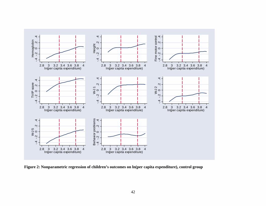
42

-.4-.2

0.2

.4H

emog

lobi

n

2.8 3 3.2 3.4 3.6 3.8 4ln(per capita expenditure)

-.4-.2

0.2

.4H

eigh

t

2.8 3 3.2 3.4 3.6 3.8 4ln(per capita expenditure)

-.4-.2

0.2

.4Fi

ne m

otor

con

trol

2.8 3 3.2 3.4 3.6 3.8 4ln(per capita expenditure)

-.4-.2

0.2

.4TV

IP s

core

2.8 3 3.2 3.4 3.6 3.8 4ln(per capita expenditure)

-.4-.2

0.2

.4W

-J 1

2.8 3 3.2 3.4 3.6 3.8 4ln(per capita expenditure)

-.4-.2

0.2

.4W

-J 2

2.8 3 3.2 3.4 3.6 3.8 4ln(per capita expenditure)

-.4-.2

0.2

.4W

-J 5

2.8 3 3.2 3.4 3.6 3.8 4ln(per capita expenditure)

-.4-.2

0.2

.4B

ehav

ior p

robl

ems

2.8 3 3.2 3.4 3.6 3.8 4ln(per capita expenditure)

Figure 2: Nonparametric regression of children’s outcomes on ln(per capita expenditure), control group

43

-.4

-.2

0.2

.4H

emog

lobi

n

2.8 3 3.2 3.4 3.6 3.8 4ln(per capita expenditure)

-.4

-.2

0.2

.4H

OM

E s

core

2.8 3 3.2 3.4 3.6 3.8 4ln(per capita expenditure)

-.4

-.2

0.2

.4M

ater

nal d

epre

ssio

n

2.8 3 3.2 3.4 3.6 3.8 4ln(per capita expenditure)

-.4

-.2

0.2

.4M

othe

r's p

erce

ived

stre

ss

2.8 3 3.2 3.4 3.6 3.8 4ln(per capita expenditure)

Figure 3: Nonparametric regression of mother’s outcomes on ln(per capita expenditure), control group

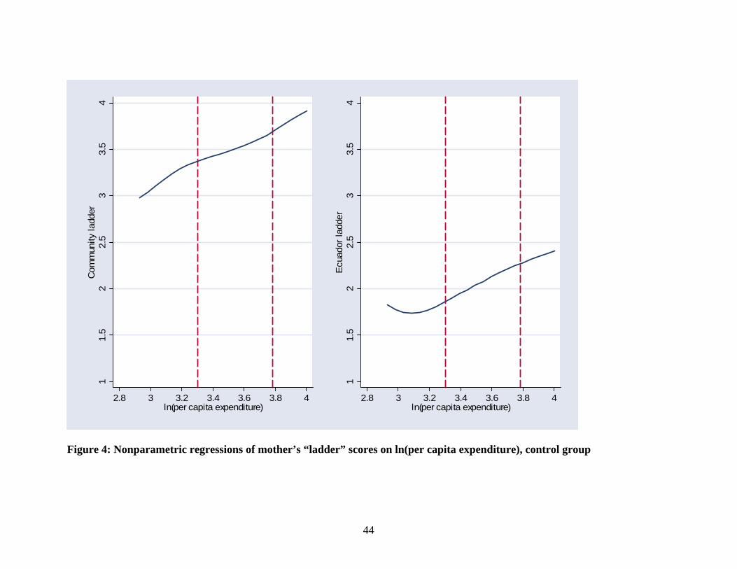
44

11.

52

2.5

33.

54

Com

mun

ity la

dder

2.8 3 3.2 3.4 3.6 3.8 4ln(per capita expenditure)

11.

52

2.5

33.

54

Ecu

ador

ladd

er

2.8 3 3.2 3.4 3.6 3.8 4ln(per capita expenditure)

Figure 4: Nonparametric regressions of mother’s “ladder” scores on ln(per capita expenditure), control group

45

-.4-.2

0.2

.4H

emog

lobi

n

2.8 3 3.2 3.4 3.6 3.8 4ln(per capita expenditure)

-.4-.2

0.2

.4H

eigh

t

2.8 3 3.2 3.4 3.6 3.8 4ln(per capita expenditure)

-.4-.2

0.2

.4Fi

ne m

otor

con

trol

2.8 3 3.2 3.4 3.6 3.8 4ln(per capita expenditure)

-.4-.2

0.2

.4TV

IP s

core

2.8 3 3.2 3.4 3.6 3.8 4ln(per capita expenditure)

-.4-.2

0.2

.4W

-J 1

2.8 3 3.2 3.4 3.6 3.8 4ln(per capita expenditure)

-.4-.2

0.2

.4W

-J 2

2.8 3 3.2 3.4 3.6 3.8 4ln(per capita expenditure)

-.4-.2

0.2

.4W

-J 5

2.8 3 3.2 3.4 3.6 3.8 4ln(per capita expenditure)

-.4-.2

0.2

.4B

ehav

ior p

robl

ems

2.8 3 3.2 3.4 3.6 3.8 4ln(per capita expenditure)

Figure 5: Nonparametric regressions of children’s outcomes on ln(per capita expenditure) Note: The dashed line is for the treatment group; expenditure is measured as baseline expenditure plus the average BDH transfer. The solid line is for the control group; expenditure is measured baseline expenditure.

46

Table 1: Comparison of families which were eligible and ineligible for the sample Former Bono Solidario

recipients Newly eligible

Observations 26,231 9,573

% of row 73.3% 26.7% At least one child age 6 or older

Average Selben score (standard deviation)

37.75 (6.28)

36.97 (7.35)

Observations 4,456 17,987

% of row 19.9% 80.2% No children age 6 or older

Average Selben score (standard deviation)

43.37 (4.85)

42.49 (5.05)

Note: These computations are for the group of 58,247 urban and rural families who were in Selben quintiles 1 & 2 and had at least one child in the household of any age, making them BDH-eligible. This group is classified into those who are former Bono recipients and those who are newly eligible for the BDH (across the columns), and those who had at least 1 child age 6 and older and those who had no children age 6 or older (down the rows). Our sample was drawn from the17,987 families in the bottom right portion of the table: newly eligible families with no children age 6 or older.

47

Table 2: Descriptive baseline statistics: analysis sample Full sample Families in lowest quartile

Treatment Control P-value, diff Treatment Control P-value,

diff

Family-level variables (observations=1,124 in full sample, 268 in lowest quartile)

imputed per capita expenditure 36.68

(0.79) 38.39 (1.10) 1.58 21.57

(0.34) 22.13 (0.54) 0.78

ln(imputed per capita expenditure) 3.54

(0.02) 3.57

(0.03) 0.35 3.05 (0.02)

3.08 (0.03)

0.40

Mother’s age in years 23.74 (0.13)

23.81 (0.27) 0.82 23.2

(0.26) 23.28 (0.44)

0.89

Mother’s education in years 7.01 (0.16)

6.79 (0.29) 0.51 6.28

(0.20) 6.16

(0.39) 0.79

Mother living with husband 0.70 (0.02)

0.67 (0.03) 0.50 0.48

(0.04) 0.49

(0.07) 0.95

# Family members 4.79 (0.11)

4.73 (0.18) 0.77 7.19

(0.24) 7.25

(0.37) 0.90

Months between interviews 22.61 (0.29)

22.47 (0.35) 0.75 22.72

(0.36) 23.15 (0.34)

0.38

Child-level variables (observations=1,479 in full sample, 365 in lowest quartile)

Indicator: Child is male 0.49 (0.01)

0.53 (0.02) 0.17 0.48

(0.03) 0.53

(0.04) 0.25

Child’s age in months 39.10 (0.65)

38.40 (0.74) 0.48 38.68

(1.02) 38.96 (1.20)

0.86

Child’s height-for-age z-score (US norms) –1.12

(0.08) –1.11 (0.14) 0.97 –1.28

(0.15) –1.39 (0.17)

0.64

Child’s hemoglobin (g/dl) 10.43 (0.08)

10.36 (0.10) 0.58 10.34

(0.12) 10.43 (0.19)

0.69

Child’s TVIP score (standardized) 81.25

(0.74) 82.91 (1.70) 0.37 78.60

(1.27) 77.05 (1.81)

0.49

Notes: The sample consists of the group of children ages 3 to 7 (and their families) for whom all 8 child outcomes studied in this paper are non-missing. Standard errors, in parentheses, are clustered at the parish level. The child’s baseline hemoglobin is elevation adjusted. The child’s baseline TVIP score has been normed according to instructions from the test developer (M=100, SD=15). Note that the baseline TVIP is available only for the subsample of children who were at least 36 months of age at baseline.

48

Table 3: Treatment effects: children’s outcomes

Controls for age and gender Controls for age, gender and

baseline family characteristics

Elevation-adjusted hemoglobin 0.116 (0.111) 0.117

(0.102)

Height 0.043 (0.058) 0.034

(0.050)

Fine motor control 0.160 (0.076) 0.171

(0.074)

TVIP score (receptive vocabulary) 0.011 (0.108) 0.021

(0.099)

WJ-1 score (long-term memory) 0.192 (0.105) 0.230

(0.106)

WJ-2 score (short-term memory) 0.034 (0.102) 0.029

(0.098)

WJ-5 (visual integration) 0.119 (0.100) 0.145

(0.072)

Behavior problems scale 0.150 (0.103) 0.146

(0.099)

Mean effect sizes

Physical measures 0.106 (0.049) 0.107

(0.040)

Cognitive and behavioral measures 0.101 (0.071) 0.114

(0.060)

All measures 0.103 (0.056) 0.112

(0.045)

Observations 1,479 1,389

Note: All dependent variables have been converted to z-scores by subtracting the sample median and dividing by the standard deviation. The measures of fine motor control and behavior problems have had their signs reversed so that higher values correspond to better outcomes (i.e. better fine motor control and fewer behavior problems). The sample is restricted to all children ages 3 to 7 years at follow-up, for whom all eight outcomes are measured. The controls for baseline family characteristics include the natural logarithm of imputed family expenditure, an indicator for whether the mother lived with a husband at baseline, the mother’s years of education and age, indicators for the numbers of family members in 5 age ranges (0 to 5, 6 to 14, 15 to 44, 45 to 64 and 64 or older) crossed with gender, and the mother’s TVIP score. Standard errors are clustered at the parish level. .

Table 4: Treatment effects with baseline expenditure interactions: children’s outcomes

Controls for age and gender Controls for age, gender and baseline family characteristics

Treated x bottom quartile

Treated x Top 3

quartiles

Bottom Quartile

Treated x bottom quartile

Treated x Top 3

quartiles

Bottom Quartile

Elevation-adjusted hemoglobin 0.390 (0.123)

0.024 (0.128)

–0.271 (0.137)

0.379 (0.130)

0.027 (0.120)

–0.232 (0.148)

Height 0.051 (0.092)

0.038 (0.060)

–0.110 (0.073)

0.041 (0.084)

0.035 (0.053)

0.027 (0.072)

Fine motor control 0.288 (0.117)

0.118 (0.072)

–0.107 (0.080)

0.270 (0.118)

0.134 (0.071)

–0.045 (0.093)

TVIP score (receptive vocabulary) 0.177 (0.148)

–0.049 (0.099)

–0.330 (0.090)

0.108 (0.142)

–0.024 (0.091)

–0.292 (0.088)

WJ-1 score (long-term memory) 0.228 (0.109)

0.179 (0.122)

–0.102 (0.109)

0.219 (0.096)

0.237 (0.127)

0.066 (0.120)

WJ-2 score (short-term memory) 0.157 (0.148)

–0.008 (0.107)

–0.145 (0.116)

0.092 (0.133)

0.006 (0.104)

–0.065 (0.109)

WJ-5 (visual integration) 0.297 (0.160)

0.053 (0.095)

–0.414 (0.141)

0.252 (0.133)

0.090 (0.076)

–0.335 (0.129)

Behavior problems scale 0.389 (0.159)

0.075 (0.113)

–0.065 (0.147)

0.389 (0.166)

0.072 (0.104)

0.002 (0.164)

Mean effect sizes

Physical measures 0.243 (0.065)

0.060 (0.049)

–0.163 (0.058)

0.230 (0.065)

0.066 (0.041)

–0.083 (0.061)

Cognitive and behavioral measures 0.250 (0.101)

0.050 (0.072)

–0.211 (0.088)

0.212 (0.093)

0.076 (0.063)

–0.125 (0.087)

All measures 0.247 (0.080)

0.054 (0.055)

–0.193 (0.072)

0.219 (0.074)

0.072 (0.045)

–0.109 (0.070)

Note: 1,479 observations without extended controls, and 1,389 observations with extended controls. The sample is restricted to all children ages 3 to 7 years at follow-up for whom all eight outcomes are measured. All dependent variables are measured as z-scores by subtracting the sample median and dividing by the standard deviation. The measures of fine motor control and behavior problems have had their signs reversed, so that higher values correspond to better outcomes (i.e. better fine motor control and fewer behavior problems). The baseline family characteristics are listed in the note to Table 3. Standard errors are clustered at the parish level.

Table 5: Robustness checks

Largest sample possible for each outcome

Published norms with analysis sample (obs:

1,448)

Obs. Treated x 1st quartile

Treated x Top 3

quartiles Treated x

1st quartile

Treated x Top 3

quartiles

Hemoglobin 1,763 0.270 (0.111)

0.047 (0.126) 0.391

(0.130) 0.032

(0.128) Height / Height-for-age Z score (for US norms) 2,157 0.015

(0.082) –0.012 (0.051) 0.063

(0.158) 0.106

(0.105)

Fine motor control 2,116 0.148 (0.096)

0.074 (0.061) 0.275

(0.112) 0.124

(0.073) TVIP score (receptive vocabulary) 2,020 0.113

(0.124) –0.046 (0.089) 0.233

(0.208) –0.070 (0.138)

WJ-1 score (long-term memory) 2,096 0.136

(0.097) 0.124

(0.103) 0.242 (0.103)

0.146 (0.143)

WJ-2 score (short-term memory) 2,067 0.091

(0.136) –0.047 (0.098) 0.146

(0.157) –0.037 (0.129)

WJ-5 (visual integration) 1,948 0.229 (0.149)

–0.012 (0.083) 0.084

(0.094) 0.102

(0.098)

Behavior problems 2,160 0.246 (0.142)

0.018 (0.100) 0.378

(0.161) 0.060

(0.112)

Mean effect sizes

Physical measures 0.144 (0.058)

0.022 (0.047) 0.243

(0.072) 0.087

(0.054) Cognitive & behavioral measures 0.163

(0.088) 0.008

(0.063) 0.217 (0.095)

0.040 (0.081)

All measures 0.156 (0.070)

0.013 (0.049) 0.227

(0.075) 0.058

(0.060)

Note: Dependent variables are measured as z-scores by subtracting the sample median and dividing by the standard deviation. The measures of fine motor control and behavior problems have had their signs reversed, so that higher values correspond to better outcomes (i.e. better fine motor control and fewer behavior problems). Standard errors are clustered at the parish level. The sample using published norms has 31 fewer observations than the sample used in Table 4 because, in these cases, one or more outcomes took on values that could not be normed using the published tables.

Table 6: Extensions: mean effect sizes by child age, gender, and education of the mother

Treated x 1st quartile

Treated x Top 3

quartiles 1st quartile Treated x

1st quartile

Treated x Top 3

quartiles 1st quartile

By age: 3 and 4 year olds 5, 6, and 7 year olds

Physical measures 0.310 (0.095)

0.028 (0.054)

–0.233 (0.073)

0.181 (0.081)

0.092 (0.057)

–0.093 (0.083)

Cognitive & behavioral measures

0.249 (0.086)

0.027 (0.073)

–0.202 (0.084)

0.251 (0.137)

0.072 (0.085)

–0.219 (0.115)

All measures 0.272 (0.078)

0.027 (0.055)

–0.214 (0.070)

0.225 (0.100)

0.080 (0.064)

–0.172 (0.090)

By sex: Girls Boys

Physical measures 0.252 (0.083)

0.130 (0.056)

–0.180 (0.064)

0.242 (0.075)

–0.008* (0.056)

–0.147 (0.072)

Cognitive & behavioral measures

0.390 (0.116)

0.063 (0.081)

–0.287 (0.093)

0.113* (0.121)

0.039 (0.079)

–0.142 (0.109)

All measures 0.338 (0.094)

0.088 (0.063)

–0.247 (0.076)

0.162 (0.095)

0.021 (0.057)

–0.144 (0.087)

By mother’s education: Incomplete primary or less Complete primary or more

Physical measures 0.319 (0.110)

–0.012 (0.057)

–0.294 (0.108)

0.217 (0.077)

0.072* (0.049)

–0.121 (0.067)

Cognitive & behavioral measures

0.140 (0.115)

–0.163 (0.080)

–0.213 (0.089)

0.292 (0.110)

0.091** (0.073)

–0.219 (0.098)

All measures 0.207 (0.097)

–0.106 (0.059)

–0.243 (0.081)

0.264 (0.090)

0.084** (0.056)

–0.182 (0.081)

Notes: Asterisks indicate that the hypothesis of equality of the coefficient for boys (older children) and girls (younger children) can be rejected at the 5% level (*) or the 1% level (**). The results are based on regressions that pool boys and girls (older and younger children) but permit the coefficients on the treatment-expenditure interactions and the indicator of being in the 1st quartile to differ across boys and girls (older and younger children). Four observations were dropped in the regressions by mother’s education due to missing values for education at baseline. All regressions include an indicator for the child’s sex and a complete set of month-of-age indicators. Standard errors are clustered at the parish level.

52

Table 7: Program effects on maternal health, parenting and health care

obs. Treated x 1st quartile

Treated x top 3 quartiles 1st quartile

Outcomes for mothers

Ecuador ladder 1,094 0.743 (0.201)

0.163 (0.175)

–0.564 (0.139)

Community ladder 1,089 1.081 (0.434)

0.336 (0.297)

-0.764 (0.269)

Hemoglobin- z-score 1,098 0.331 (0.154)

0.141 (0.132)

–0.189 (0.121)

Depressive symptoms- z-score 915 0.212 (0.163)

–0.002 (0.085)

–0.046 (0.140)

Perceived stress- z-score 1,046 –0.034 (0.114)

–0.074 (0.082)

–0.201 (0.105)

HOME score- z-score 1,117 0.323 (0.238)

–0.042 (0.135)

–0.399 (0.178)

Health care and schooling outcomes Child had growth control in last 6 months (mean=0.368) 1,479 0.042

(0.062) 0.059

(0.044) -0.079 (0.049)

Child had parasite treatment in last 12 months (mean=0.592) 1,476 0.207

(0.059) 0.103

(0.044) -0.139 (0.047)

Child in a preschool or grade school (mean=0.447) 1,479 0.062

(0.061) 0.035

(0.045) –0.109 (0.042)

Notes: Regressions for mother’s outcomes control for the age of the mother (in 10-year age bands). Regressions for children control for the child’s age and gender. Standard errors are clustered at the parish level. The measures of depressive symptoms, perceived stress, and the HOME score are coded so that higher values correspond with better outcomes.

53

Table 8: Respondent’s report of what BDH transfers were spent on

All Most A little None

Food 19.21 30.02 30.19 20.58

Health 3.04 4.83 24.51 67.62

Housing 0.90 1.26 4.33 93.50

Education 4.29 6.44 23.79 65.47

Transportation --- 0.72 38.81 60.47

Clothes 4.51 6.86 22.74 65.88

Goods for husband -- -- 1.65 98.35

Note: Mothers were asked “How much of the bono was spent on [item listed I first column]?” Each row of the table shows the distribution of mothers’ responses to these questions. The sample consists of all mothers of children in the analysis sample who reported receiving BDH transfers.

Table 9: Tests of Engel curve hypothesis

Expected ln(per capita expenditure) x

Indicator: Treated Treated Control

Test 1: (2)=(3), p-value

Test 2: (2)=(3)

and (1)=0. p-value

(1) (2) (3)

All quartiles

Physical outcomes 0.627 (0.261)

0.053 (0.044)

0.201 (0.061) 0.042 0.008

Cognitive and behavioral outcomes

0.424 (0.426)

0.106 (0.063)

0.199 (0.097) 0.420 0.323

All outcomes 0.500 (0.335)

0.087 (0.047)

0.199 (0.078) 0.211 0.113

Poorest expenditure quartile

Physical outcomes 2.484 (0.812)

–0.051 (0.155)

0.664 (0.187) 0.006 0.000

Cognitive and behavioral outcomes

2.850 (0.789)

–0.278 (0.110)

0.555 (0.196) 0.001 0.000

All outcomes 2.713 (0.663)

–0.193 (0.102)

0.596 (0.162) 0.000 0.000

Notes: The estimates shown are based on estimates of equation (4). A complete set of indicators for the age in months of the child were included, as was an indicator for the child’s sex. Standard errors are clustered at the parish level.

55

Appendix Table 1: Baseline characteristics of all children at baseline, children in both baseline and follow-up surveys, and children in the analysis sample. Baseline

Follow-up Analysis sample

Mean Obs Mean Obs Mean Obs Household and mother’s characteristics

Imputed log expenditure 3.48 1,561 3.48 1,553 3.50 1,124

Mother’s age in years 23.62 1,656 23.63 1,551 23.77 1,122

Mother’s education in years 6.80 1,654 6.83 1,549 6.94 1,120

Mother living with husband 0.692 1,658 0.690 1,553 0.688 1,124

# family members 4.74 1,658 4.75 1,553 4.77 1,124

In treatment group 0.665 1,658 0.672 1,553 0.680 1,124

Months between interviews 22.58 1,553 22.57 1,124

Received bono (bank records) 0.568 1,513 0.574 1,100

Received bono (reported) 0.567 1,553 0.573 1,124

Children’s characteristics

Indicator: child is male 0.501 2,359 0.505 2,204 0.502 1,479

Child’s age in months 37.49 2,359 37.43 2,204 38.88 1,479 Child’s height-for-age z-score (US norms) -1.225 2,255 -1.219 2,111 -1.12 1,419

Child’s hemoglobin 10.39 2,098 10.38 1,968 10.41 1,323 Child’s standardized TVIP score 81.45 1,169 81.66 1,087 799 81.78

Notes: Only children at baseline who would have been between ages 36 and 95 months at follow-up are included in this analysis. Ages for children lost at follow-up were imputed based on mean number of months between baseline and follow-up in each parish. The child’s TVIP is measured only for children who were at least 36 months old at baseline.

56

Appendix Table 2: Means (standard deviations) of outcome variables by whether any child outcome is missing

No missing outcomes (obs=1,479)

At least one missing outcome

Mean (Std.Dev) Mean (Std.Dev) Obs

Test of equality;

t-stat (p-value)

Age in months 61.41 (14.19)

56.96 (14.44) 718 5.74

(0.00)

Hemoglobin –0.024 (1.000)

–0.183 (0.988) 284 .77

(0.44)

Height 0.149 (0.990)

–0.152 (0.992) 678 1.52

(0.13)

Fine motor control –0.080 (0.922)

–0.445 (1.120) 637 4.35

(0.00) TVIP score (receptive vocabulary)

0.381 (0.999)

0.072 (0.968) 541 2.76

(0.01) WJ-1 score (long-term memory)

0.268 (0.994)

–0.028 (0.986) 617 3.65

(0.00) WJ-2 score (short-term memory)

–0.037 (0.929)

–0.497 (1.093) 588 5.77

(0.00)

WJ-5 (visual integration) –0.020 (0.988)

–0.098 (1.037) 469 0.70

(0.49)

Behavior problems –0.041 (0.993)

–0.003 (01.015) 681 0.43

(0.67) Note: All child outcomes except age have been converted to z-scores, and the signs of fine motor control and behavior problems have been reversed so that higher values correspond to better outcomes. The last column shows t-tests for whether the mean for the sample with no missing outcomes is equal to that for the sample with missing outcomes. For all variables except age, variables are age- and sex- adjusted, i.e. the test is based on a regression of each variable on an indicator for whether the child has at least one missing outcome, a complete set of age indicators, and an indicator of the child is male. These regressions have standard errors that are clustered at the parish level.