Chapter 8: Exchange

8.1: Introduction In many ways this chapter is the most important in the book. If you have time to study just one, this is the one that you should study (even though it might be a bit difficult studying it on its own). It has a brilliant idea in it (the Edgeworth Box) and it generates an exciting number of important results. It is used over and over again in the rest of the book. It is exciting and insightful because it portrays in a very simple way the benefits people get out of exchanging things. It shows what exchanges (if any) are possible, what exchanges are efficient and which are not, and what exchanges may take place under different institutions. It shows that what economists call perfect competition has some nice properties, while monopoly and monopsony have some less-than-nice properties.

8.2: Exchange We consider a really simple story. We have an economy in which there are just two individuals and just two goods. Call the individuals A and B and the goods 1 and 2. The economy is a simple pure-exchange economy – nothing is produced – the individuals wake up in the morning to find that they each have an endowment of each of the two goods. They could, if they want, simply consume their initial endowments – or they may find it mutually convenient to do some kind of trade or exchange between the two of them. The purpose of this chapter is to see whether it might be possible to have some mutually advantageous trade – and, if so, whether we can offer some advice as to how it might be carried out. Obviously the answers to these questions depend upon the preferences of the individuals and their initial endowments. We shall start with a particular example and then we shall try and generalise the results we have obtained. Later we shall present several more specific examples.

8.3: Individual A’s Preferences and Endowments Although we work with a particular example you should pay attention to the general principles we are using. We start with a statement of Individual A’s preferences and endowments, though perhaps that should be preceded by a statement of the space in which we will be representing these preferences and endowments. This will be the same as we have been using for the last 3 chapters: with the quantity of good 1, denoted by q1, along the horizontal axis and the quantity of good 2, denoted by q2, along the vertical axis. We assume in this example that A has an initial endowment of 22 units of good 1 and 92 units of good 2. Further we assume that A’s preferences over these two goods are Cobb-Douglas with parameter a = 0.7. This enables us to draw A’s indifference curves and endowment point in the following figure. Note that the endowment point is indicated with the letter E – it is at the point (22, 92).

You will note that we have drawn the indifference curve passing through the initial endowment point. This enables us to answer the question: to where in this space would individual A voluntarily move? The answer is simple: anywhere above and to the right of the indifference curve passing through the point E.

8.4: Individual B’s Preferences and Endowments We now do the same for Individual B. Here we assume that he or she starts with an initial endowment of 128 units of good 1 and 8 units of good 2. We assume that B also has Cobb-Douglas preferences but here with a weight of just 0.6 on good 1. So B absolutely prefers good 1 but relative to A prefers good 2. We draw B’s indifference curves and endowment point:

Note that B starts at (128, 8). In the figure is the indifference curve passing through the initial point. B would be happy to move to any point above and to the right of this indifference curve.

8.5: The Edgeworth Box We now do one of the clever things that Edgeworth did – he first turned Individual B upside down! This gives us:

Let us carefully consider what this means. For B his or her origin – the zero point – is at the top right hand corner of this figure. The quantity of good 1 that B has is measured from this top right hand corner leftwards – so the horizontal distance from the top right hand corner to the endowment point E is 128 units – the endowment that B has of good 1. Moreover, the quantity of good 2 that B has is measured from this top right hand corner downwards – so the vertical distance from the top right hand corner to the endowment point E is 8 units – the endowment that B has of good 2. Obviously the further to the left and the further down the happier is Individual B – so his or happiness increases as we move from the top right hand corner – his origin – down and to the left. In this figure lower indifference curves mean more happiness for individual B. It follows that B would be happy to move to any point in this space to the left of and below the indifference curve passing through the initial endowment point E. We note that A starts with 22 of good 1 and 92 of good 2, while B starts with 128 of good 1 and 8 of good 2. Between the two of them they have a grand total of 150 of good 1 and 100 of good 2. The problem that we are going to discuss is the division of these 150 units of good 1 and 100 units of good 2 between the two of them – given, of course, their initial allocation. To help us in this discussion we shall use a brilliant device – named the Edgeworth Box after its originator. We have already described one of the clever things that Edgeworth did – namely turn B upside down – we now describe the second clever thing that he did. He superimposed figure 8.3 on top of figure 8.1 in such a way that the initial endowment points coincided.

What do we note: the width of this box is the sum of the horizontal distance from A’s origin to the endowment point (A’s endowment of good 1 - 22 units) plus the horizontal distance from B’s origin to the endowment point (B’s endowment of good 1 - 128 units). That is the width of the box is the total amount of good 1 that the two individuals possess between them. That is, 150 units. We also note that the height of this box is the sum of the vertical distance from A’s origin to the endowment point (A’s endowment of good 2 - 92 units) plus the vertical distance from B’s origin to the endowment point (B’s endowment of good 2 - 8 units), That is the height of the box is the total amount of good 2 that the two individuals possess between them. That is, 100 units. So the dimensions of the box are determined by the total amounts of the two goods that society (the two individuals together) have of the two goods. The width is the total amount of good 1; the height the total amount of good 2. Now note that every point in the box is an allocation of the goods between the two members of society. For example, point E is the initial allocation. The bottom origin (0, 0) represents an allocation in which A gets nothing and B gets everything. The top origin (150, 100) represents an allocation in which A gets everything and B gets nothing. The mid-point (75, 50) represents an allocation in which A ends up with 75 units of good 1 and 50 of good 2 – and so does B – they split the total up evenly. And so on. The question is: what happens? Are they happy to stay where they are – at point E? Or might they be better off moving to some other point in the space? We have already seen that A would be happy moving to any point to the right and above his or her indifference curve passing though E; similarly B would be happy moving to any point to the left and below his or her indifference curve passing though E. A glance at the figure shows that there is quite a large region to which both of them would be happy to move. Can we narrow things down a bit?

8.6: The Contract Curve

If you look at the figure you will see that there are points of tangency between the indifference curves of A and those of B. If we join them up we get a very important curve – which is known as the contract curve. As its name suggests, it indicates the points where some kind of contract, some kind of deal, some kind of exchange, between A and B might be made. Why? First of all, let us understand its properties. Take any indifference curve of individual A and ask yourself – “where on this indifference curve for A is B happiest?”

What is your answer? The point where there is an indifference curve of B tangential to that of A – and this point, by definition, is on the contract curve. Now do the converse: take any indifference curve of individual B and ask yourself – “where on this indifference curve for B is A happiest?” The answer? The point where there is an indifference curve of A tangential to that of B – and this point, by definition, is on the contract curve1. So the contract curve is the locus of points efficient in the sense that, for any given level of utility for individual A the utility of B is maximised, and for any given level of utility for individual B the utility of A is maximised. It follows that points off the contract curve are inefficient. What does this mean? Simply that, from any point off the contract curve, there is always some direction in which we can move and increase the utility of at least one of the individuals without decreasing the utility of the other2. To show this, take any point off the contract curve and then move towards the contract curve – by moving between an indifference curve of A and an indifference curve of B. Starting at point E provides an obvious example: what happens if we move from E towards the contract curve by moving between A’s original indifference curve and B’s original indifference curve? The utility of both increase. This is true no matter where we start from – as long as it is off the contract curve. However, once we are on the contract curve, we can no longer increase the utility of one individual without decreasing the utility of the other. Try it.

1 The contract curve is not necessarily the locus of tangency points. What it is the locus of points efficient in the sense that will very shortly be defined. 2 Actually we can usually say something stronger: that there is always some direction in which we can move and increase the utility of both of the individuals.

So the contract curve is the locus of efficient points. Points off the contract curve are inefficient in the sense that we can usually make both individuals better off by moving away and towards the contract curve. It seems reasonable then to conclude that any contract made between the two individuals should be on the contract curve. We have narrowed things down a lot: it seems that we can conclude that any contract should be on the contract curve, between the point where A’s original indifference curve intersects it and the point where B’s original indifference curve intersects it. (For neither would accept a deal that made them worse off than at the initial point.) Can we narrow things down any further? One way we can narrow things down further is by imposing a particular trading institution and looking at the implications. An obvious choice – particularly in view of chapter 2 – is that institution which economists call perfect competition. Essentially this is the imposition of a price, which both individuals take as given, which is such that demand and supply are equal. In the context of this chapter, it is the imposition of a price for which both individuals are happy to move to the same point in the box. If such a price exists, then both are happy to move to the same point and this point is the chosen allocation. Does such a price exist?

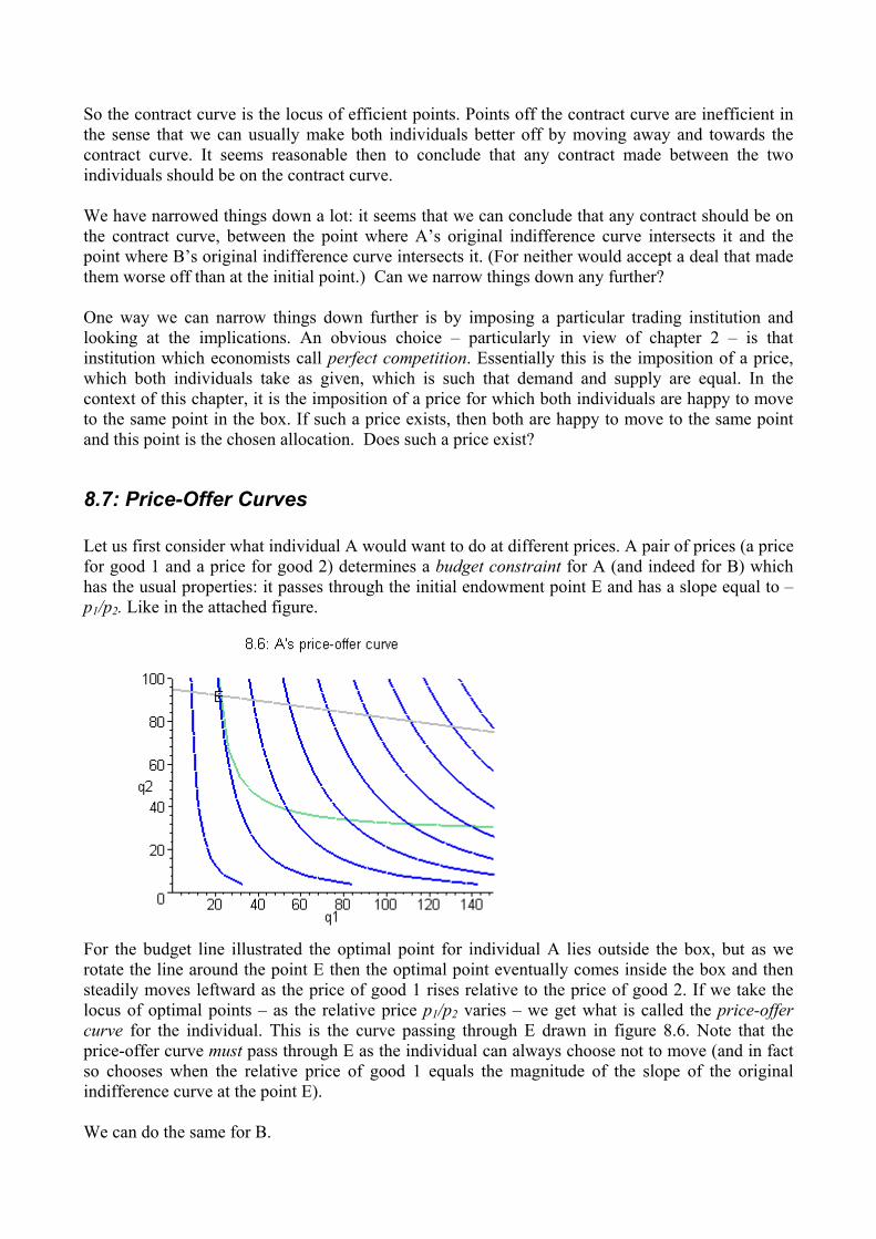
8.7: Price-Offer Curves Let us first consider what individual A would want to do at different prices. A pair of prices (a price for good 1 and a price for good 2) determines a budget constraint for A (and indeed for B) which has the usual properties: it passes through the initial endowment point E and has a slope equal to –p1/p2. Like in the attached figure.

For the budget line illustrated the optimal point for individual A lies outside the box, but as we rotate the line around the point E then the optimal point eventually comes inside the box and then steadily moves leftward as the price of good 1 rises relative to the price of good 2. If we take the locus of optimal points – as the relative price p1/p2 varies – we get what is called the price-offer curve for the individual. This is the curve passing through E drawn in figure 8.6. Note that the price-offer curve must pass through E as the individual can always choose not to move (and in fact so chooses when the relative price of good 1 equals the magnitude of the slope of the original indifference curve at the point E). We can do the same for B.

Here a particular budget constraint is shown (the straight line through E) and it is clear that the optimal point is on the price-offer curve for B (the curve through E). Once again the price-offer curve passes through E as the individual can always choose not to move.

8.8: Competitive Equilibrium Let us now put the two price-offer curves together and ask whether there is a point where they intersect. If there is, then this is the competitive equilibrium that we have been looking for.

There is such a point – and it is on the contract curve! That is interesting (and good news) – but is it surprising? Let us call the competitive equilibrium point C. It is the intersection of the two price-offer curves. We know that C is on the price-offer curve of A. This means that the budget constraint through the initial point pictured in the above figure must be tangential to A’s indifference curve at that point. Similarly, we know that C is on the price-offer curve of B. This means that the budget constraint through the initial point pictured in the above figure must be tangential to B’s indifference curve at that point. If the budget line is tangential to A’s indifference curve and to B’s it must therefore follow that A’s indifference curve is tangential to B’s at the point C. It follows that C must be on the contract curve. It is not surprising. We thus have a really nice result: the competitive equilibrium must be on the contract curve and must therefore be efficient. Let us note the implications. The initial point has A with 22 units of good 1 and 92 of good 2, and B with 128 of good 1 and 8 of good 2. As you will see from the figure above, the competitive equilibrium is at the point (70, 36) as measured from the bottom left origin and is at the point (80, 64) as measured from the top right origin. In this competitive equilibrium A has 70 of good 1 and 36 of good 2, and B has 80 of good 1 and 64 of good 2. It might be easiest to see all of this in a tabular form.

Initial allocation Individual A Individual B Society Good 1 22 128 150 Good 2 92 8 100

Competitive

equilibrium allocation Individual A Individual B Society

Good 1 70 80 150 Good 2 36 64 100

Changes between the

two allocations Individual A Individual B Society

Good 1 +48 -48 0 Good 2 -56 +56 0

What happens is that Individual B gives 48 units of good 1 to Individual A in exchange for 56 units of good 2 – which Individual A gives to Individual B. The rate of exchange is 48 units of good 1 for 56 units of good 2. The slope of the line joining E and C determines this exchange rate – this slope is – 56/48 – this is of course –p1/p2. So p1/p2 = 56/48 = 1.16666. Good 1 is more expensive than good 2 in the sense that for each unit of good 1 exchanged the return is more than one unit of good 2. You might like to ask why the exchange is the way it is – why A gives good 2 to B and B gives good 1 to A. You could simply say that A starts out with lots more of good 2 and B starts out with lots more of good 1. But it is more to do with where the initial point is in relation to the contract curve. Indeed you might like to ask why the contract curve is where it is – why is to the right and below the line joining the two origins. This is a consequence of the fact that the two individuals have different preferences – with B relatively (to A) preferring good 2. (Note that both individuals absolutely prefer good 1 – their values of a are greater than 0.5 – but A’s is 0.7 while B’s is 0.6, so relative to A¸ individual B prefers good 2. That is the reason the contract curve is where it is.)

8.9: Price-Setting Equilibria We have investigated above one market institution – that of competitive equilibrium. Each agent takes the price as given and we ask whether there is a price at which both individuals want to move to the same point. If so, we have found a competitive equilibrium. Now we explore other trading institutions. In particular we explore what happens if we give to one of the individuals the ability to choose the price (the exchange rate). The other individual simply takes the price as given and chooses the point to which they will move. This binds the first mover (the price setter) to accept that point. What happens? Suppose we give to Individual A the right to choose the price. He or she knows that then Individual B will choose the point to which he or she wants to move – and this binds them both. What does A do? We can argue in this fashion. Given any choice of the price by A, individual B will respond by choosing the point on his or her price-offer curve. So, in essence, A is choosing a point on B’s price-offer curve. What point does he or she choose? Consider the figure:

B’s price-offer curve is the curve going through point E. If A can choose any point on this, which point does he or she choose? Obviously the best point on it relative to A’s indifference curves. Which is the highest point from that point of view? Point A – it is on the highest possible A indifference curve. So if A can choose the price, he or she chooses the budget line going from E through A. Given this budget line, B’s best response is to choose point A. Point A is approximately (64, 72) as measured from the bottom left origin and (86, 28) as measured from the top right origin. In tabular form:

Initial allocation Individual A Individual B Society Good 1 22 128 150 Good 2 92 8 100

Allocation determined by A setting the price

Individual A Individual B Society

Good 1 64 86 150 Good 2 72 28 100

Changes between the

two allocations Individual A Individual B Society

Good 1 +42 -42 0 Good 2 -20 +20 0

Note what happens – in this allocation A gives 20 units of good 2 to B in exchange for 42 units of good 1. Compared to the competitive equilibrium it is obviously a much better deal for individual A. This is hardly surprising – as it was chosen by A. So it is better for A and worse for B. But there is something else. What do we see from the figure above? That the point chosen by A setting the price – point A – is off the contract curve. It is inefficient! This means that there is some direction from point A in which the individuals can move which makes both of them better off. Why do they not do that? Simply because A is choosing the price – not the point. If he or she could choose a point then A would choose the point on the contract curve just below where it intersects B’s original indifference curve. But choosing a price is not the same as choosing a point: choosing a price is choosing a direction to move from point E.

For completeness we also present the case when B sets the price and A responds by choosing the point – but you can probably anticipate the result. In this case, B is effectively choosing a point on A’s price-offer curve. Which point does he or she choose?

B chooses the point on A’s price-offer curve (the curve through the point E) which is best from B’s point of view. B therefore chooses point B – by asking a budget line given by the line going from E through B. What do we notice about point B? First, it implies the following trades:

Initial allocation Individual A Individual B Society Good 1 22 128 150 Good 2 92 8 100

Allocation determined by B setting the price

Individual A Individual B Society

Good 1 42 108 150 Good 2 45 55 100

Changes between the

two allocations Individual A Individual B Society

Good 1 +20 -47 0 Good 2 -47 +20 0

In this exchange, A gives 47 units of good 2 to B – in exchange for 20 units of good 1. Compared to the competitive equilibrium it is obviously a much better deal for individual B. This is hardly surprising – as it was chosen by B. Like the point chosen by A however point B is off the contract curve – it is inefficient – and for the same reasons. So price-setting (monopoly or monopsony) by one of the two agents is inefficient - whereas perfect competition is efficient. That is why governments like competition.

8.10: Two Theorems of Welfare Economics

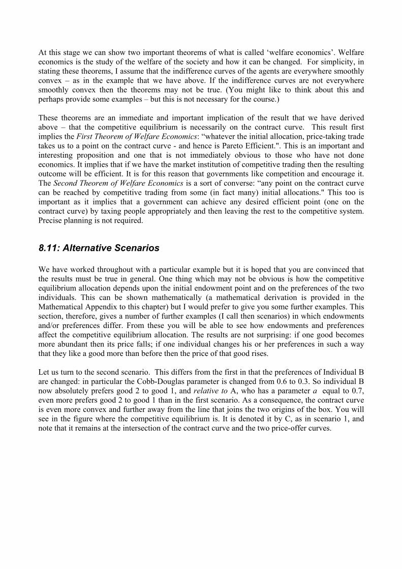
At this stage we can show two important theorems of what is called ‘welfare economics’. Welfare economics is the study of the welfare of the society and how it can be changed. For simplicity, in stating these theorems, I assume that the indifference curves of the agents are everywhere smoothly convex – as in the example that we have above. If the indifference curves are not everywhere smoothly convex then the theorems may not be true. (You might like to think about this and perhaps provide some examples – but this is not necessary for the course.) These theorems are an immediate and important implication of the result that we have derived above – that the competitive equilibrium is necessarily on the contract curve. This result first implies the First Theorem of Welfare Economics: “whatever the initial allocation, price-taking trade takes us to a point on the contract curve - and hence is Pareto Efficient.". This is an important and interesting proposition and one that is not immediately obvious to those who have not done economics. It implies that if we have the market institution of competitive trading then the resulting outcome will be efficient. It is for this reason that governments like competition and encourage it. The Second Theorem of Welfare Economics is a sort of converse: “any point on the contract curve can be reached by competitive trading from some (in fact many) initial allocations." This too is important as it implies that a government can achieve any desired efficient point (one on the contract curve) by taxing people appropriately and then leaving the rest to the competitive system. Precise planning is not required.

8.11: Alternative Scenarios We have worked throughout with a particular example but it is hoped that you are convinced that the results must be true in general. One thing which may not be obvious is how the competitive equilibrium allocation depends upon the initial endowment point and on the preferences of the two individuals. This can be shown mathematically (a mathematical derivation is provided in the Mathematical Appendix to this chapter) but I would prefer to give you some further examples. This section, therefore, gives a number of further examples (I call then scenarios) in which endowments and/or preferences differ. From these you will be able to see how endowments and preferences affect the competitive equilibrium allocation. The results are not surprising: if one good becomes more abundant then its price falls; if one individual changes his or her preferences in such a way that they like a good more than before then the price of that good rises. Let us turn to the second scenario. This differs from the first in that the preferences of Individual B are changed: in particular the Cobb-Douglas parameter is changed from 0.6 to 0.3. So individual B now absolutely prefers good 2 to good 1, and relative to A, who has a parameter a equal to 0.7, even more prefers good 2 to good 1 than in the first scenario. As a consequence, the contract curve is even more convex and further away from the line that joins the two origins of the box. You will see in the figure where the competitive equilibrium is. It is denoted it by C, as in scenario 1, and note that it remains at the intersection of the contract curve and the two price-offer curves.

In this competitive equilibrium A ends up with more of good 1 than in scenario 1 – and we note that the budget line (joining E and C) is flatter – so that the equilibrium price of good 1 is lower. This follows because B likes good 1 less than before. In scenario 3 we give the two individuals identical tastes (but the same endowments as in scenario 1). It follows that the contract curve is the straight line joining the two origins. With Cobb-Douglas preferences this is always the case3. We thus have:

3 Indeed it is always true with identical homothetic preferences. (Though you do not need to know what homothetic preferences are.) They are defined in the Mathematical Appendix.

The competitive equilibrium is on this line joining the two origins – so that A gets some 40% of the total quantity of good 1 and 40% of the total quantity of good 2, while B gets around 60%. In this scenario A does relatively badly as he or she starts with rather little of good 1 – the good that both of the individuals prefer. Scenario 4 is the same as scenario 1 in terms of preferences but the endowments are rearranged so that A starts out with most of good 1 and B starts out with most of good 2.

You will see that the competitive equilibrium sort of corrects this. Scenario 5 has the same endowments as Scenario 4 but gives the two individuals the same preferences so that the contract curve is the straight line joining the two origins.

Once again the competitive equilibrium is on this line. The next 3 scenarios are interesting in that we return to the same totals as in Scenario 1 (150 units of good 1 and 100 units of good 2) but we assume that individual A starts out with all 100 units of good 2 while B starts out with all 150 units of good 1. This is an interesting case in that the price-offer curve of A is horizontal while that for B is vertical. Why? Consider individual A. Suppose his or her Cobb-Douglas parameter is a. Suppose he or she has an initial endowment of zero of good 1 and e2 of good 2. Then the value of his income is p2e2 and we know that he or she wants to spend a fraction a of this on good 1 and a fraction (1-a) on good 2. We thus have his demands:

q1 = ap2e2/p1 and q2 = (1-a)p2e2/p2 from which we get

q1 = ap2e2/p1 and q2 = (1-a)e2 Note what the second of these says: that the demand for good 2 is constant, independent of the prices, and is always equal to a fixed fraction of the initial endowment. In Scenario 6 A’s parameter a is 0.7 and therefore A always wants to spend a fraction 30% of his initial endowment of good 2. His initial endowment of good 2 is 100 and therefore he or she always wants 30 units of good 2. He or she sells the rest (70 units) and buys as many units of good 1 as he or she can with this. Hence the horizontal price-offer curve for individual A. A similar argument applies for B. If his or her value of the parameter is a and if he or she starts with an endowment of e1 units of good 1 and zero units of good 2, then the value of his or her income is p1e1. His or her demands are therefore:

q1 = ap1e1/p1 and q2 = (1-a)p1e1/p2

from which we get

q1 = ae1 and q2 = (1-a)p1e1/p2

from which we note that the demand for good 1 is constant, independent of the prices. In Scenario 6 a for B is 0.6 and so he or she always spends 60% of his or her endowment of good 1 on good 1. The endowment is 150 units – therefore his demand for good 1 is constant at 90 units. He sells the remaining 60 units and buys as many units of good 2 as possible with this. Thus his or her price-offer curve is vertical at the value 60 (= 150 – 90). (Recall that we measure B from the top right origin.) Scenario 6 looks as follows:

We should note that the preferences – and hence the contract curve – and the total endowments of the two goods are the same as in Scenario 1. What differs is how the endowments are initially allocated. We have a different allocation – so we have a different competitive equilibrium. Scenario 7 is to Scenario 2 as Scenario 6 is to Scenario 1: just the initial distribution differs. Scenario 7 is:

Similarly, Scenario 8 is to Scenario 3 as Scenario 6 is to Scenario 1: just the initial allocation differs. We have:

Note that the two individuals have identical tastes – so that the contract curve is the straight line joining the two origins.

8.12: Comments It should be clear that there are almost always possibilities for exchange. Only when the initial allocation point lies on the contract curve are such possibilities absent. Even when the preferences are identical (so that the contract curve joins the two origins of the box) there will usually be the possibility of trade – unless the initial point is on the contract curve (for example when the endowments are identical so that we start at the middle point of the box). Also even when the endowments are identical (so that the initial point is in the centre of the box) there will usually be the possibility of trade – unless the contract curve also goes through the centre of the box (for example, when preferences are identical). So, as long as people are different we will generally have mutually advantageous trade. This chapter paid particular attention to the competitive trading mechanism – showing that it is efficient and leads to trade on the contract curve. We also saw that price-setting (monopoly or monopsony) behaviour is inefficient. There are obviously other trading mechanisms – and you might like to consider what their properties are.

8.13: Summary We have done a lot in this chapter. We have considered the general problem of exchange between two individuals and have used the clever device of the Edgeworth Box to examine this.

We have discovered the contract curve. The contract curve is the locus of points efficient in the sense that, once on the contract curve, it is impossible to make one person better off without making the other worse off. Points off the contract curve are inefficient in the sense that there is always some movement which makes at least one person better off without making the other worse off. We have shown that the competitive equilibrium is on the contract curve. The two price-offer curves must intersect on the contract curve. The competitive equilibrium is on the contract curve and hence is efficient in the above sense. Price-setting equilibria (in which one agent sets the price and the other chooses the point) is inefficient. Moreover and very importantly: The competitive equilibrium depends upon the preferences and the endowments.

8.14: Is equality good? Is planning good? There are two propositions that might be considered self-evident. The first is that equality is a good thing - and hence that inequality is a bad thing. The second is that planning an economy is good for the people in the society - and hence that leaving people open to market forces is bad. While these propositions are certainly true in some instances, we explore here whether there are situations in which they are not true. We use the apparatus of this chapter and consider a very simple pure-exchange economy in which there are just two individuals. The individuals, crucially, are different. There are two goods in this society, Good 1 and Good 2, and two individuals, Individual A and Individual B. We assume that there is available in the society a quantity of 100 units of Good 1 and a quantity of 100 units of Good 2 to allocate between the two individuals. We ask whether the allocation of 50 units of each good to each individual – and the enforced consumption of these quantities – is a good thing or not. That is, is planning plus equality necessarily a Good Thing? We assume that the individuals are different in their preferences. Specifically we assume that Individual A has Cobb-Douglas preferences with parameter 0.7 (that is, weight 0.7 on Good 1 and weight 0.3 on Good 2) while Individual B has Cobb-Douglas preferences with parameter 0.3 ((that is, weight 0.3 on Good 1 and weight 0.7 on Good 2). So Individual A relatively prefers Good 1 while Individual B relatively prefers Good 2. Having a difference in the preferences is important and drives what follows. If the preferences were identical then the two propositions that we are looking at are rather self-evident. But we know that in the real world people are different. We use the apparatus of this chapter to investigate the allocation of the 100 units of Good 1 and the 100 units of Good 2 between the two individuals. We use an Edgeworth Box of size 100 by 100, in which we measure Individual A’s consumption from the bottom left-hand origin and Individual B’s consumption from the top right-hand corner of the box. Every point within the box is an allocation

of the 100 units of Good 1 and the 100 units of Good 2 between the two individuals. Consider a planned allocation in which both individuals are given and consume 50 units of each good. This allocation is at the centre of the box – point E in the figure below. The question is: are the two individuals happy to stay at this point – or would they prefer to be “exposed to market forces”. The answer depends on what these ‘market forces’ are. If we have a competitive market, in which each individual takes the price as given and we seek for an equilibrium price (at which both individuals would agree to a particular exchange), we can see that the answer must be ‘yes’. The competitive equilibrium of this allocation problem is at the point labelled C in this figure: it is on the contract curve and is at the intersection of the two price-offer curves. Note that at C, Individual A consumes 70 of Good 1 and 30 of Good 2, while Individual consumes 30 of Good 1 and 70 of Good 2. Note that in equilibrium the relative price of the two goods is 1 – the slope of the line joining E with C is –1. You might like to ask where these numbers (70 and 30, 30 and 70) come from (recall the preferences of the two individuals). We end up at an unequal allocation – having started at an equal planned allocation – and both individuals prefer the unequal allocation to the equal allocation. Inequality is not necessarily bad. Market forces are not necessarily bad.

Indeed, you might like to argue that point C is in a sense the best allocation in the box – we started with an equal allocation and we ended up (after trading at the competitive price) at a point they both prefer to the initial allocation. It is interesting to note that we could end up at this ‘best’ point even if we have an initial allocation that is clearly not the same for the two individuals. For example, suppose we start with A having all 100 units of the good he or she relatively dislikes (Good 2) and with B having all 100 units of the good that he or she relatively dislikes (Good 1). See the following figure. Notice also that in both equilibria the implicit prices of the two goods are equal – their

relative price (minus the slope of the line joining the endowment point and the equilibrium point) is 1.

It is further clear that it does not matter where we start, as long as it is one some point on the equilibrium budget constraint – the line joining the top left-hand corner of the box with the bottom right-hand corner. It is interesting to note that at each point on this line, the values of the endowments of the two individuals are equal (at the equilibrium price ratio). So we could argue that this is truly a fair – if not necessarily equal (in terms of consumption) – situation: start at any point on this equilibrium budget constraint and let the competitive market do the rest. A planner obviously could also find the point C if it knew the preferences of the two individuals. Clearly the point C depends on the preferences, and if the planner miscalculates the preferences then it will miscalculate the point C. One advantage of the market solution is that the government does not really need to know the preferences of the two individuals – it just needs to start them off on the equilibrium budget constraint. In a sense this is cheating since the equilibrium budget constraint is also dependent on the preferences (here we have chosen an example in which the equilibrium price ratio just happens to be 1, but this does not need to be the case). Nevertheless the government can try and start the two individuals at the centre of the box, and leave the competitive market to do the rest. We end up (if the individuals have different preferences) at a necessarily unequal consumption point – but one we might argue is ‘fair’. There are other qualifications we should make, particularly to what we mean by market forces. If one of the two individuals can set the price, then it may well be the case that we end up at an unsatisfactory equilibrium. Perhaps you would like to think about this case.

8.15: Mathematical Appendix Here we provide a solution to the general problem of competitive exchange between two individuals with Cobb-Douglas preferences. Let us denote the endowments (e1,e2) for individual A and (f1,f2) for individual B. Let us suppose that A has Cobb-Douglas preferences with parameter a and that B has Cobb-Douglas preferences with parameter b. Do recall that the parameter indicates the relative weight that the individual places on good 1 – the relative weight put on good 2 is one minus this parameter. From the material in Chapter 6, we know that A’s gross demands for the two goods are:

q1 = a(p1e1 + p2e2/p1 and q2 = (1-a)(p1e1 + p2e2)/p2

while B’s gross demands are

q1 = b(p1f1 + p2f2)/p1 and q2 = (1-b)(p1f1 + p2f2)/p2 From these we can calculate the aggregate gross demand for good 1 and impose the market-clearing equilibrium condition that the aggregate gross demand should equal the aggregate supply of good 1, which is e1 + f1. This gives us the equilibrium condition:

a(p1e1 + p2e2)/p1 + b(p1f1 + p2f2)/p1 = e1 + f1 This is an equation which can be solved for the price ratio p1/p2 which gives equilibrium in the market for good 1. Solving it yields:

p2/p1 = [(1-a)e1 + (1-b)f1]/(ae2 + bf2) (8.1) Before discussing the implications of this, let us also derive the market-clearing condition for good 2. Imposing the condition that the aggregate gross demand equals the supply of good 2, we have:

(1-a)(p1e1 + p2e2)/p2 + (1-b)(p1f1 + p2f2)/p2 = e2 + f2

If we solve this for the implied equilibrium price ratio p2/p1 we get….equation (8.1)! Is this a surprise? Clearly not – as if the market for good 1 is in equilibrium then so must be the market for good 2. (You should check this out. Suppose the equilibrium in the market for good 1 has A giving x units to A and B receiving x units from A, then it must be the case that A is getting in exchange y units of good 2 and B is giving in exchange y units of good 2, where p1x = p2y.) Now let us examine the equilibrium condition, after noticing that it is a condition on the relative prices of good 1 and good 2 (which determines the slope of the equilibrium budget constraint). From (8.1) above we see that p2/p1 increases if either of e1, f1 increase and p2/p1 decreases if any of e2, f2, a or b increases

The first of these says that if good 1 becomes more plentiful then its relative price decreases. The second says: (1) that if good 2 becomes more plentiful then its relative prices decreases; and (2) that if good 1 becomes more preferred by either individual (either a or b increases) then the relative price of good 1 increases; (3) that if good 2 becomes more preferred by either individual (either a or b decreases) then the relative price of good 2 increases. All of these accord with intuition.