chapter 10 factors affecting the rate of genetic changeusers.tamuk.edu/kfsdl00/chapter...
TRANSCRIPT

I. Elements of the Key Equation for Genetic Change
II. The Key Equation in More Precise Terms
III. Trade-Offs Among Elements of the Key Equation
IV. Comparing Selection Strategies Using the Key Equation
V. The Key Equation in Perspective
VI. Male Versus Female Selection
Chapter 10 – Factors Affecting the Rate of Genetic Change

Learning Objective: To understand the factors (heritability, intensity of selection, phenotypic variation, and generation interval) that affect the predicted amount of genetic progress, and how certain factors can be manipulated by the breeder.
Chapter 10 – Factors Affecting the Rate
of Genetic Change

I. Elements of the Key Equation for Genetic
Change
The Key Equation: Four Factors Accuracy of Selection – A measure of the strength of the relationship between true breeding values and their predictions for a trait under selection (largely a function of heritability). Selection Intensity – A measure of how “choosy” breeders are in deciding which individuals are selected. Genetic Variation – Variability of breeding values within a population for a trait under selection. This is the key to genetic progress. Generation Interval – The average amount of time required to replace one generation with the next.

II. The Key Equation in More Precise Terms
^ rBV,BV i σBV
∆BV/t = ________ L where ∆BV/t = predicted rate of genetic change per unit of time
^ rBV,BV = accuracy of selection
i = selection intensity
σBV = genetic variation
L = generation interval

^
rBV,BV i σBV
∆BV/t = ________
L
where ∆BV/t = The predicted change in mean breeding value of a population due to selection. Only BV is passed on from selected parents to offspring.
^ rBV,BV = The strength of the relationship between true breeding values and their predictions for a trait under selection. Accuracy ranges from 0 (no information) to 1 (lots of information).
i = selection intensity (phenotypic difference between the mean selection criterion of those individuals selected to be parents and the population mean = the “Standardized Selection Differential”).
σBV = genetic variation (the standard deviation of breeding values).
L = generation interval (the average age of parents when their selected offspring are born).


L = generation interval (the average age of parents when their selected offspring are born). Generally, the larger the size of the species, the longer the generation interval. TABLE 10.2 Common generation intervals (modified) Generation Interval Species (years) Horses 8 to 12 Dairy cattle 4 to 6 Beef cattle 4 to 6 Sheep/Goats 3 to 5 Swine 1.5 to 2 Chickens/Rabbits 1 to 1.5


III. Trade-Offs Among Elements of the Key Equation
^
rBV,BV i σBV
∆BV/t = ________
L Accuracy vs. Generation Interval – To wait for more progeny records to enhance accuracy would increase the generation interval. A strategy is to choose the better young sires with the highest accuracies and use for only one year. Accuracy vs. Intensity – Likewise, to wait for more progeny records to enhance accuracy for only a few sires would decrease the intensity of selection (i.e., the percentage selected). One solution is to test more sires that have fewer progeny records. Intensity vs. Generation Interval – Being too choosy usually results in a longer generation interval. However, the real trade-off is between selecting females vs. males (e.g., a lower replacement rate dictates that animals remain longer in the population). Intensity vs. Risk – A problem may exist if very few sires are used that have low accuracies, whereby their breeding values turn out to be poorer than what was initially reported.

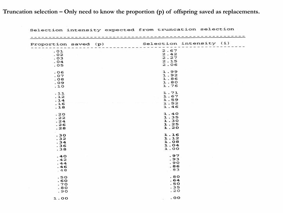
Truncation selection – Only need to know the proportion (p) of offspring saved as replacements.

___ __ __
_ SCS - SC
i = _______
σSC
Truncation selection – Only need to know the proportion (p) of offspring saved as
replacement.

Mathematical Proof of the Key Equation:
Given the following parameters for a sheep population being selected for yearling weight
(YW, lbs): μ = 130 Mean of selected males = 190 and females = 158 lbs
h2 = 0.36 σP = 30 lbs L = 3 years
1) R = h2 x SD = 0.36 x (174 – 130) {SD (Selection Differential) = 44 lbs
R = 15.84 lbs
_ _
2) R = h2 i σP {i = “Standardized Selection Differential”
_
= 0.36 x 1.465 x 30 = i = SD/σP ; 44/30 = 1.465
R = 15.84 lbs
ˆ _
3) rBV, BV i σBV { = h2 x σ2P = σ2
BV = 0.36 x 302 = 324 (√ 324 = 18)
∆BV/t = __________
L
_
= √ h2 i σBV = √.36 x 1.465 x 18 = 15.84 = 5.28 lbs/yr
______________ ______________________ ______
L 3 3

IV. Comparing Selection Strategies Using the Key Equation

___ __ __
_ SCS - SC
i = _______ = 9.43 – 5.0 = 2.215
σSC √4
i = “Standardized Selection Differential”
Mathematical proof of i : = “Standardized Selection Differential”
Determine the intensity of selection values (i) for each sex.
Top 1% (p) of males; i = 2.67 Top 10% (p) of females; i = 1.76
Mean of i = (2.67+1.76)/2 = 2.215
Mean of selected males: μ + iσ Mean of selected females: μ + iσ
5.0 + 2.67(√4.0) = 10.34 kg 5.0 + 1.76(√4.0) = 8.52 kg
__
Mean of selected offspring : SCS
__
SCS = 10.34 + 8.52 = 9.43 kg
2

IV. Comparing Selection Strategies Using the Key Equation
Mean of i = (2.67+1.76)/2 = 2.215
{∆BV = R, genetic “response” to selection}
∆BV = √.35 x 2.215 x √ 1.4
= 1.55 kg
New mean = 5.0 + 1.55
= 6.55 kg
{σ2BV = h2 x σ2
p}
= .35 x 4
= 1.4
σBV = √ 1.4
= 1.1832
R/t = 1.55/1.5 = 1.034 kg/year

IV. Comparing Selection Strategies Using the Key Equation
Problem 10.1: Calculate the rate of genetic change in feed conversion in a
swine population given the following:
Heritability of feed conversion (h2) = .35
Phenotypic standard deviation (σp) = .2 lb/lb
Accuracy of male selection (rBVm,BVm) = .8
Accuracy of female selection (rBVf,BVf) = .5
Intensity of male selection (im) = -2.4
Intensity of female selection (if) = -1.5
Generation interval for males (lm) = 1.8 years
Generation interval for females (lf) = 1.8 years

IV. Comparing Selection Strategies Using the Key Equation (Problem 10.1):
^
rBV,BV i σBV
∆BV/t = _________
L
^
^
(rBVm,BVmim + rBVf,BVf
if) σBV
= _______________________
Lm + Lf
= (.8(-2.4) + .5(-1.5))(.118) = -.088 lb/lb/year
1.8 + 1.8

IV. Comparing Selection Strategies Using the Key Equation
Problem 10.6: A rancher runs a closed herd of breeding cattle. He normally
keeps and breeds the top 3% of his bull calves based on individual performance for
yearling weight (YW). His sires average three years of age when their offspring are
born. He is studying two female replacement strategies:
Saving the top 20% of his heifers based on YW (Lf = 6.2 years)
Saving the top 60% based on YW (Lf = 3.2 years; cull more older cows)
a. If h2YW = .5, and σPYW
= 60 lb, calculate the expected annual rate of genetic change in YW for each strategy. Strategy 1:
b. What elements of the key equation is the rancher experimenting with?
c. What element appears to be more important?
^
^
(rBVm,BVmim + rBVf,BVf
if) σBV
∆BV/t = _______________________ = (.7071(2.27) + .7071(1.4))(42.4264) = 11.97 lb/yr
Lm + Lf 3.0 + 6.2

IV. Comparing Selection Strategies Using the Key Equation
A rancher runs a closed herd of breeding cattle. He normally keeps and breeds the
top 3% of his bull calves based on individual performance for yearling weight (YW).
His sires average three years of age when their offspring are born. He is studying
two female replacement strategies:
Saving the top 20% of his heifers based on YW (Lf = 6.2 years)
Saving the top 60% based on YW (Lf = 3.2 years ; cull more older cows)
a. If h2YW = .5, and σPYW
= 60 lb, calculate the expected rate of genetic change in YW for each strategy. Strategy 2:
b. What elements of the key equation is the rancher experimenting with?
if and Lf
c. What element appears to be more important?
The i affects L (i.e., by culling more cows that are aged or less productive, if increases, which potentially can translate into more genetic progress).
^
^
(rBVm,BVmim + rBVf,BVf
if) σBV
∆BV/t = _______________________ = (.7071(2.27) + .7071(.64))(42.4264) = 14.08 lb/yr
Lm + Lf 3.0 + 3.2
