c 614 acta - oulu

UNIVERSITY OF OULU P .O. Box 8000 F I -90014 UNIVERSITY OF OULU FINLAND

A C T A U N I V E R S I T A T I S O U L U E N S I S

University Lecturer Tuomo Glumoff

University Lecturer Santeri Palviainen

Postdoctoral research fellow Sanna Taskila

Professor Olli Vuolteenaho

University Lecturer Veli-Matti Ulvinen

Planning Director Pertti Tikkanen

Professor Jari Juga

University Lecturer Anu Soikkeli


Publications Editor Kirsti Nurkkala

ISBN 978-952-62-1553-2 (Paperback)ISBN 978-952-62-1554-9 (PDF)ISSN 0355-3213 (Print)ISSN 1796-2226 (Online)

U N I V E R S I TAT I S O U L U E N S I SACTAC

TECHNICA


TECHNICA

OULU 2017

C 614

Antti Roivainen

THREE-DIMENSIONAL GEOMETRY-BASED RADIO CHANNEL MODEL: PARAMETRIZATION AND VALIDATION AT 10 GHZ

UNIVERSITY OF OULU GRADUATE SCHOOL;UNIVERSITY OF OULU,FACULTY OF INFORMATION TECHNOLOGY AND ELECTRICAL ENGINEERING;CENTRE FOR WIRELESS COMMUNICATIONS;INFOTECH OULU

C 614

AC

TAA

ntti Roivainen

C614etukansi.kesken.fm Friday, April 7, 2017 3:12 PM

ACTA UNIVERS ITAT I S OULUENS I SC Te c h n i c a 6 1 4

ANTTI ROIVAINEN


Academic dissertation to be presented with the assent ofthe Doctoral Training Committee of Technology andNatural Sciences of the University of Oulu, for publicdefence in Kaljusensali (KTK112), Linnanmaa, on 17 May2017, at 12 noon

UNIVERSITY OF OULU, OULU 2017

Copyright © 2017Acta Univ. Oul. C 614, 2017

Supervised byProfessor Matti Latva-aho

Reviewed byProfessor Andreas F. MolischProfessor Bernard H. Fleury

ISBN 978-952-62-1553-2 (Paperback)ISBN 978-952-62-1554-9 (PDF)

ISSN 0355-3213 (Printed)ISSN 1796-2226 (Online)

Cover DesignRaimo Ahonen

JUVENES PRINTTAMPERE 2017

OpponentProfessor Luis M. Correia

Roivainen, Antti, Three-dimensional geometry-based radio channel model:parametrization and validation at 10 GHz. University of Oulu Graduate School; University of Oulu, Faculty of Information Technologyand Electrical Engineering; Centre for Wireless Communications; Infotech OuluActa Univ. Oul. C 614, 2017University of Oulu, P.O. Box 8000, FI-90014 University of Oulu, Finland

Abstract

This dissertation presents complete parameterizations for a three-dimensional (3-D) geometry-based stochastic radio channel model (GSCM) at 10 GHz based on measurement campaigns. Thethesis is divided into the following main parts: radio channel measurements, the characterizationof model parameters, and model validation.

Experimental multiple-input multiple-output (MIMO) channel measurements carried out intwo-story lobby and urban small cell scenarios are first described. The measurements wereperformed with a vector network analyzer and dual polarized virtual antenna arrays with abandwidth over 500 MHz. The measurement data was post-processed using the ESPRIT algorithmand the post-processed data was verified using a semi-deterministic map-based model. The resultsshowed a good match between estimated and modeled multipath components (MPCs). In addition,single-input single-output outdoor-to-indoor measurements were executed through a standardmulti-pane glass window and concrete wall.

A statistical analysis was carried out for defining full 3-D characterization of the propagationchannel in both line-of-sight (LOS) and non-line-of-sight (NLOS) propagation conditions. Thedelay and angular dispersions of MPCs are smaller in comparison to lower frequency bands dueto the higher attenuation of the delayed MPCs. Moreover, specular reflection is observed to be themore dominant propagation mechanism in comparison to diffuse scattering, leading to smallercluster angle spreads in comparison to lower frequency bands. The penetration loss caused by astandard multi-pane glass window is on the same level as in the lower frequency bands, whereasthe loss caused by the concrete wall is a few dBs higher than at lower frequency bands.

Finally, the GSCM with determined parameters is validated. A MIMO channel wasreconstructed by embedding 3-D radiation patterns of the antennas into the propagation pathestimates. Equivalently the channel simulations were performed with a quasi deterministic radiochannel generator (QuaDRiGa) using the defined parameters. The channel capacity, Demmelcondition number, and relative condition numbers are used as the comparison metrics betweenreconstructed and modeled channels. The results show that the reconstructed MIMO channelmatches the simulated MIMO channel well.

Keywords: GSCM, MIMO, model validation, multipath component, outdoor-to-indoor,statistical parameters, vector network analyzer, virtual antenna array

Roivainen, Antti, Roivainen, Antti, Kolmiulotteinen geometriaan perustuvastokastinen radiokanavamalli: parametrointi ja validointi 10 GHz:n taajuus-alueella. Oulun yliopiston tutkijakoulu; Oulun yliopisto, Tieto- ja sähkötekniikan tiedekunta; Centre forWireless Communications; Infotech OuluActa Univ. Oul. C 614, 2017Oulun yliopisto, PL 8000, 90014 Oulun yliopisto

Tiivistelmä

Tämä väitöskirja esittää parametroinnit kolmiulotteiselle geometriaan perustuvalle stokastiselleradiokanavamallille 10 GHz:n taajuusalueella perustuen mitattuun radiokanavaan. Väitöskirjakoostuu kolmesta pääalueesta: radiokanavamittaukset, radiokanavamallin parametrien määrittä-minen ja mallin validointi.

Aluksi kuvataan kaksikerroksisessa aula ja kaupunkipiensolu ympäristöissä monilähetinmonivastaanotin (MIMO) järjestelmällä tehdyt kanavamittaukset. Mittaukset tehtiin vektoripiiri-analysaattorilla ja kaksoispolaroiduilla virtuaaliantenniryhmillä 500 MHz kaistanleveydellä.Mittausdata jälkikäsiteltiin käyttämällä ESPRIT-algoritmia ja jälkikäsitelty data varmennettiinosittain deterministisellä mittausympäristön karttaan pohjautuvalla radiokanavamallilla. Tulok-set osoittivat hyvän yhteensopivuuden mitattujen ja mallinnettujen moniteiden välillä. Lisäksitoteuttiin yksi-lähetin yksi-vastaanotin mittaukset ulko-sisä etenemisympäristössä monikerroksi-sen lasin ja betoniseinän läpi.

Tilastollinen analyysin avulla määritettiin täysi kolmiulotteinen kuvaus radioaallon etenemis-kanavasta näköyhteys ja näköyhteydettömässä tilanteissa. Moniteiden suuremmista vaimennuk-sista johtuen viive ja kulmahajonnat ovat pienemmät verrattaessa matalempiin taajuuksiin. Peili-heijastus on diffuusisirontaa merkittävämpi radioaallon etenemismekanismi johtaen pienempiinklustereiden kulmahajeisiin matalempiin taajuuksiin verrattuna. Monikerroksisen lasin läpäisy-vaimennus on samankaltainen kuin alemmilla taajuuksilla, kun sitä vastoin betoniseinän vaimen-nus on muutaman desibelin suurempi kuin alemmilla taajuuksilla.

Lopulta geometriaan perustava stokastinen radiokanavamalli validoidaan määritellyillä para-metreilla. MIMO kanava uudelleen rakennetaan lisäämällä kolmiulotteiset antennien säteilyku-viot estimoituihin radioaallon etenemisteihin. Vastaavasti radiokanava simuloidaan näennäisestideterministisellä radiokanavageneraattorilla (QuaDRiGa) käyttäen määriteltyjä mallin paramet-reja. Kanavakapasiteettia, Demmel ehtolukua ja suhteellista ehtolukua käytetään vertailumitta-reina uudelleen rakennetun ja simuloidun kanavan välillä. Tulosten perusteella uudelleen raken-nettu MIMO kanava on yhteensopiva simuloidun radiokanavan kanssa.

Asiasanat: GSCM, mallin validation, MIMO, monitiekomponentti, tilastollisetparametrit, ulko-sisä etenimisympäristö, vektoripiirianalysaattori,virtuaaliantenniryhmä

To My Family

Preface

Research for this thesis has been carried out at the Centre for Wireless Communications(CWC), at the University of Oulu, Finland, during the years 2015–2016. After finalizinga Master’s thesis in 2007, it was difficult to find a suitable research topic for a doctoralthesis. Finally, after changing research topic a couple of times, my supervisor ProfessorMatti Latva-aho gave me the topic of radio channel modeling at 10 GHz in 2015. Thistopic perfectly fitted my earlier research experience in the field of channel measurementsand modeling. Therefore, I am grateful to him for finding me a suitable research topicand pushing me forward in my doctoral studies.

I would also like to thank Professor Markku Juntti for giving me the opportunity tobroaden my knowledge in the field of wireless communications in his research groupduring the years 2009–2013. I would further like to thank Professor Aarno Pärssinenand Dr. Markus Berg, who were the members of the follow-up group in my doctoralstudies, for giving me numerous practical tips concerning my thesis. I also wish toexpress my gratitude to the pre-examiners of this thesis Professor Andreas F. Molischfrom the University of Southern California, USA, and Professor Bernard H. Fleury fromthe University of Aalborg, Denmark. Their comments significantly improved the qualityof the thesis.

I would like to thank all the personnel at the CWC including my superiors, colleaguesand fellow researchers for creating an open and inspiring working environment duringmy stay at CWC. My thanks go especially to our channel modeling group and myco-authors in publications, Veikko Hovinen, Pekka Kyösti, Dr. Marko Sonkki, andNuutti Tervo. I am also grateful to Claudio Ferreira Dias, PhD, for implementing thepropagation path estimation tool and for co-authorizing publications. I want to alsothank Docent Erkki Salonen for the technical support and Marko Wirtanen for assistingin outdoor-to-indoor and outdoor channel measurements. The administrative support ofJari Sillanpää, Hanna Saarela, Kirsi Ojutkangas, Eija Pajunen, and Mari Lehmikangas isalso highly appreciated.

During the years at CWC, I have had the privilege to work on several researchprojects and get to know numerous colleagues. The projects were funded by differentassociations. For instance, ESTEC funded the Assessment of the C-Band Satellite-to-Indoor Propagation and Shadowing by Vegetation (ASIPS) and the Propagation Effects

9

for Mobile Multimedia Services (PROBMOB) projects. The European Commissionfunded the project Mobile and wireless communications Enablers for the Twenty-twentyInformation Society (METIS). The Finnish Funding Agency for Technology andInnovation (Tekes) funded several projects, namely, Cooperative MIMO Techniquesfor Cellular System Evolution (COMIT), Baseband and System Technologies forWireless Evolution (BASE), Solutions for capacity crunch in wireless access withflexible architectures (CRUCIAL), 5G radio access solutions to 10 GHz and beyondfrequency bands (5Gto10G). In the Tekes projects, the main industrial funders wereNokia, Nokia Networks, Electrobit, Anite Telecoms, Renesas Mobile Europe, andKeysight Technologies. The work done in all projects was a highly educational process.Therefore, I would also like to thank all project managers and dozens of colleaguesin these projects. During 2016, I was encouraged to apply for several personal grantapplications and I was fortunate to receive personal grants from a number of Finnishfounding organizations: Tauno Tönning foundation, Jenny and Antti Wihuri foundation,and Riitta and Jorma J. Takanen foundation. These founding organizations are highlyappreciated.

My deepest gratitude goes to my parents, Maija and Olavi, who first encouraged meto apply to university and later urged me to pursue even higher education. I want to alsothank my parents-in-law, Sari and Jouko, for taking care our two daughters wheneverneeded when I was working during the weekends. Finally, I want to thank my wife Terhifor supporting me during my studies and our two lovely daughters, Noora and Iida, forhelping to forget work matters when I spent precious time with them.

Oulu, April 2017 Antti Roivainen

10

Abbreviations

aHHl,m modeled complex channel amplitude between horizontal received polar-

ization and horizontal transmitted polarizationaHV

l,m modeled complex channel amplitude between horizontal received polar-ization and vertical transmitted polarization

aVHl,m modeled complex channel amplitude between vertical received polariza-

tion and horizontal transmitted polarizationaVV

l,m modeled complex channel amplitude between vertical received polariza-tion and vertical transmitted polarization

a++m estimated complex channel amplitude between +45◦ received polariza-

tion and +45◦ transmitted polarizationa+−m estimated complex channel amplitude between +45◦ received polariza-

tion and −45◦ transmitted polarizationa−+m estimated complex channel amplitude between −45◦ received polariza-

tion and +45◦ transmitted polarizationa−−m estimated complex channel amplitude between −45◦ received polariza-

tion and −45◦ transmitted polarizationaHH

m estimated complex channel amplitude between horizontal receivedpolarization and horizontal transmitted polarization

aHVm estimated complex channel amplitude between horizontal received

polarization and vertical transmitted polarizationaVH

m estimated complex channel amplitude between vertical received polar-ization and horizontal transmitted polarization

aVVm estimated complex channel amplitude between vertical received polar-

ization and vertical transmitted polarizationB bandwidthb time constantC(t,n f )

[1] instantaneous channel capacity with fixed SNRC(t,n f )

[2] instantaneous channel capacity with fixed transmission powerc speed of lightcφ cluster azimuth angle spreadcθ cluster elevation angle spread

11

D K-S test statisticd distance between the transmitter and receiverd⊥ perpendicular distance from the outdoor transmitter to the external walld0 reference distancedin distance from the external wall to the indoor receiverdout distance from outdoor transmitter to the wall penetration pointdRx,nr three-dimensional position vector of the receiver antenna elementdTx,nt three-dimensional position vector of the transmitter antenna elemente Napier’s constantFθ ,Rx,nr vertical radiation field pattern of nrth antenna element of receiver antennaFθ ,Tx,nt vertical radiation field pattern of nt th antenna element of transmitter

antennaFφ ,Rx,nr horizontal radiation field pattern of nrth antenna element of receiver

antennaFφ ,Tx,nt horizontal radiation field pattern of nt th antenna element of transmitter

antennaf carrier frequencyGR gain of the receiver antennaGT gain of the transmitter antennaH time-variant time domain MIMO channelH0 null hypothesisHF time-variant frequency domain MIMO channelJ(ϑ) Jones rotation matrixKD Demmel condition numberKn relative condition numberKF1 Ricean K-factor at the initial position of the user equipmentKFt interpolated value of Ricean K-factor at the user equipment position in

the tth time instantk Boltzmann constantLb basic transmission lossL[1]

b basic transmission loss of MIMO channelL[2]

b basic transmission loss of SISO channelLF free space lossl lth clusterM number of propagation paths

12

Mi normal distributed filtered correlation map of the ith LSP including theeffect of cross-correlation matrix

M∗i normal distributed filtered correlation map of the ith LSP without theeffect of cross-correlation matrix

MFi scenario specific distributed correlation map of the ith LSP

m mth propagation path/ray/multipathN number of measured snapshotsNc number of clustersN f number of subcarriersNR number of receiver antenna elementsNs number of channel impulse response samples above the noise cut off

levelNT number of transmitter antenna elementsNTAPS maximum number of delay tapsN0 thermal noise powern path loss exponentn f subcarriernmin minimum of Tx and Rx antennasnr Receiver antenna elementnt transmitter antenna elementPl power of the lth clusterPm gain of the mth propagation pathPT transmission powerPGt path gainrRx unit vector with estimated AoA and EoArTx unit vector with estimated AoD and EoDr unit vector with modeled departure or arrival anglesSF [dB]

t interpolated value of shadow fading standard deviation in decibels at theuser equipment position in the tth time instant

T noise temperatureTS number of time samplest timeUt,n f ∈ CNr×Nr

unitary rotation matrix

13

Vt,n f ∈ CNt×Nt

unitary rotation matrixvl,m Doppler frequency component of modeled channel in mth ray of lth

clusterv(τm) Doppler frequency component of mth estimated propagation pathWe penetration loss of external wall with perpendicular grazing angleWGe penetration loss of external wall with non-perpendicular grazing angleXCC cross-correlation matrixZl random component in the power calculation for the lth clusterα coefficient showing the distance dependence on path lossαin indoor attenuation coefficientβ floating intercept path loss at reference distanceγ signal-to-noise ratioγPL Path loss dependence on carrier frequency∆ discrete grid for angle spread minimization∆BS spacing between BS antenna elements∆d change of link distanceη channel normalization factorθG grazing angleθl lth cluster elevation angleθ A

l,m modeled EoA of the mth propagation path in the lth clusterθ D

l,m modeled EoD of the mth propagation path in the lth clusterθ A

m EoA of the mth propagation pathθ D

m EoD of the mth propagation pathΘm nine-element channel parameter vector of the mth propagation pathϑ rotation angleλ0 wavelengthλi ith eigenvalueλmin(·) smallest eigenvalue of the matrix in the argumentλmax strongest eigenvalueΛn f ,t singular value matrixµ mean valueξ evaluated large-scale parameter in correlation distance analysisρx,y cross-correlation coefficient between x and y

14

σ standard deviationστ root mean square delay spread from the correlation map at user equip-

ment positionτ delayτ0 mean excess delayτm delay of the mth propagation pathτl delay of the lth clusterφl lth cluster azimuth angleφ A

l,m modeled AoA of the mth propagation path in the lth clusterφ D

l,m modeled AoD of the mth propagation path in the lth clusterφm offset angle of the mth rayφ A

m AoA of the mth propagation pathφ D

m AoD of the mth propagation pathE(·) expected value of the argument(·)T transpose operation(·)H complex conjugate transpose (Hermitian)‖ · ‖F Frobenius normeig{·} eigenvalue decompositionlog2(·) logarithm in base 2log10(·) logarithm in base 10C set of complex numbersR set of real numbersN normal distributionU uniform distribution2-D two-dimensional2G second generation3-D three-dimensional3G third generation3GPP third generation partnership project4-D four-dimensional4G fourth generation5-D five-dimensional5G fifth generation5GCM 5G channel modelAoA azimuth angle of arrival

15

AoD azimuth angle of departureAS angle spreadASA azimuth angle spread of arrivalASD azimuth angle spread of departureAWGN additive white Gaussian noiseBS base stationCDF cumulative distribution functionCEPT European Conference of Postal and Telecommunications AdministrationsCOST cooperation in science and technologyCI close-inCIR channel impulse responseCV critical valueCW continuous waveDoA direction of arrival in 3-D spaceDoD direction of departure in 3-D spaceDP dual polarizationDS RMS delay spreadECC Electronic Communications CommitteeECDF empirical cumulative distribution functionEIRP effective isotropic radiated powerEoA elevation angle of arrivalEoD elevation angle of departureESA elevation angle spread of arrivalESD elevation angle spread of departureESPRIT estimation of signal parameters via rotation invariance techniquesFCC Federal Communication CommissionFDTD finite difference time domainFI floating interceptGSCM geometry-based stochastic channel modelIF intermediate frequencyIFFT inverse fast Fourier transformi.i.d. independent and identically distributedIMT International Mobile TelecommunicationsIMT-A International Mobile Telecommunications-advancedIR impulse response

16

ISIS initial and search improved SAGEITU International Telecommunication UnionITU-R International Telecommunication Union-Radiocommunication sectorKF Ricean K-FactorK-S Kolmogorov-SmirnovLNA low noise amplifierLOS line-of-sightLSP large-scale parameterMCD multipath component distanceMETIS mobile and wireless communications enablers for the twenty-twenty

information society 5GMIMO multiple-input multiple-outputMiWEBA millimetre-wave evolution for backhaul and accessML maximum likelihoodmmMagic millimetre-wave based mobile radio access network for fifth generation

integrated communicationsNIST National Institute of Standards and TechnologyNLOS non-line-of-sightNYU New York UniversityO2I outdoor-to-indoorPA power amplifierPDP power delay profilePDF probability density functionPL path lossPLin indoor path lossPLout outdoor path lossPLtw path loss through the wallRMS root mean squareQuaDRiGa quasi deterministic radio channel generatorRF radio frequencyRMS root mean squareRT ray-tracingRx receiverSAGE space-alternating generalized expectation-maximizationSCM spatial channel model

17

SCM-E spatial channel model-extendedSF shadow fadingSISO single-input single-outputSNR signal-to-noise ratioSP single polarizationSSF small-scale fadingSSP small-scale parameterTx transmitterUE user equipmentULA uniform linear arrayURA uniform rectangular arrayUTD uniform theory of diffractionV2V vehicle-to-vehicleVNA vector network analyzerWINNER wireless world initiative new radioWLAN wireless local area networkWRC World Radiocommunication ConferenceWSS wide sense stationaryXPD cross polarization discriminationXPR cross polarization ratioXPRH cross polarization ratio for horizontal transmission polarizationXPRV cross polarization ratio for vertical transmission polarizationZoA zenith angle of arrivalZoD zenith angle of departureZSA zenith angle spread of arrivalZSD zenith angle spread of departure

18

Contents

AbstractTiivistelmäPreface 9Abbreviations 11Contents 191 Introduction 21

1.1 Motivation . . . . . . . . . . . . . . . . . . . . . . . . . . . . . . . . . . . . . . . . . . . . . . . . . . . . . . . . . . 21

1.2 Classification of radio channel models . . . . . . . . . . . . . . . . . . . . . . . . . . . . . . . . . 22

1.2.1 Analytical models . . . . . . . . . . . . . . . . . . . . . . . . . . . . . . . . . . . . . . . . . . . . . 23

1.2.2 Physical models . . . . . . . . . . . . . . . . . . . . . . . . . . . . . . . . . . . . . . . . . . . . . . . 24

1.3 Review of the GSCMs and standardized models . . . . . . . . . . . . . . . . . . . . . . . . . 26

1.3.1 Review of the GSCMs and standardized models below 6 GHz. . . . . .26

1.3.2 Channel modeling activities towards 5G . . . . . . . . . . . . . . . . . . . . . . . . . 28

1.3.3 Parameters of GSCM for frequency bands above 6 GHz . . . . . . . . . . . 30

1.4 Aims and outline of the thesis . . . . . . . . . . . . . . . . . . . . . . . . . . . . . . . . . . . . . . . . . 33

1.5 Author’s contributions to the publications . . . . . . . . . . . . . . . . . . . . . . . . . . . . . . 35

2 Fundamentals of the geometry-based stochastic channel model 372.1 Relevant terminology . . . . . . . . . . . . . . . . . . . . . . . . . . . . . . . . . . . . . . . . . . . . . . . . . 37

2.1.1 Scattering cluster . . . . . . . . . . . . . . . . . . . . . . . . . . . . . . . . . . . . . . . . . . . . . . 38

2.1.2 Channel segment and drop . . . . . . . . . . . . . . . . . . . . . . . . . . . . . . . . . . . . . 38

2.1.3 Time evolution and virtual motion . . . . . . . . . . . . . . . . . . . . . . . . . . . . . . .39

2.2 Generic model . . . . . . . . . . . . . . . . . . . . . . . . . . . . . . . . . . . . . . . . . . . . . . . . . . . . . . . 40

2.3 Overview of the parameter sets . . . . . . . . . . . . . . . . . . . . . . . . . . . . . . . . . . . . . . . . 43

2.4 Generation of channel coefficients with QuaDRiGa. . . . . . . . . . . . . . . . . . . . . . 44

2.5 Usage of the model . . . . . . . . . . . . . . . . . . . . . . . . . . . . . . . . . . . . . . . . . . . . . . . . . . 49

3 Experimental radio channel measurements 513.1 Measurement equipment and antennas . . . . . . . . . . . . . . . . . . . . . . . . . . . . . . . . . 52

3.2 MIMO measurements . . . . . . . . . . . . . . . . . . . . . . . . . . . . . . . . . . . . . . . . . . . . . . . . 53

3.2.1 Two-story lobby environment . . . . . . . . . . . . . . . . . . . . . . . . . . . . . . . . . . . 55

3.2.2 Urban small cell . . . . . . . . . . . . . . . . . . . . . . . . . . . . . . . . . . . . . . . . . . . . . . . 58

3.3 Outdoor-to-indoor SISO measurements . . . . . . . . . . . . . . . . . . . . . . . . . . . . . . . . 58

19

3.4 Post-processing . . . . . . . . . . . . . . . . . . . . . . . . . . . . . . . . . . . . . . . . . . . . . . . . . . . . . . 613.4.1 Validation of the multipath estimation . . . . . . . . . . . . . . . . . . . . . . . . . . . 64

4 Channel model parameterizations 734.1 Full 3-D parametrization . . . . . . . . . . . . . . . . . . . . . . . . . . . . . . . . . . . . . . . . . . . . . .73

4.1.1 Path loss and shadow fading . . . . . . . . . . . . . . . . . . . . . . . . . . . . . . . . . . . . 734.1.2 Large-scale parameters . . . . . . . . . . . . . . . . . . . . . . . . . . . . . . . . . . . . . . . . . 764.1.3 Cross-correlation parameters . . . . . . . . . . . . . . . . . . . . . . . . . . . . . . . . . . . .814.1.4 Correlation distances . . . . . . . . . . . . . . . . . . . . . . . . . . . . . . . . . . . . . . . . . . 844.1.5 XPR, PDP, and the delay proportionality factor . . . . . . . . . . . . . . . . . . . 864.1.6 Cluster parameters . . . . . . . . . . . . . . . . . . . . . . . . . . . . . . . . . . . . . . . . . . . . . 90

4.2 O2I path loss model . . . . . . . . . . . . . . . . . . . . . . . . . . . . . . . . . . . . . . . . . . . . . . . . . . 934.3 Discussion and conclusions related to 3-D model parameters . . . . . . . . . . . . . 98

5 Channel model validation 1035.1 Generation of MIMO transfer matrix from the post-processed data . . . . . . . 1045.2 Channel simulations with proposed model parameters . . . . . . . . . . . . . . . . . . 1055.3 Validation metrics and results . . . . . . . . . . . . . . . . . . . . . . . . . . . . . . . . . . . . . . . . 1075.4 Discussion and opportunities . . . . . . . . . . . . . . . . . . . . . . . . . . . . . . . . . . . . . . . . . 117

6 Summary and future work 123References 127

20

1 Introduction

1.1 Motivation

Over the past ten years, mobile traffic and the number of connected devices havegrown explosively. In the past, the mobile traffic was dominated by voice traffic. Asa consequence of the popularization of smartphones and tablets, mobile data traffichas now surpassed voice traffic and has grown 4,000-fold since 2005 [1]. This trendwill continue and mobile data traffic will grow exponentially [2]. Globally it has beenpredicted that the traffic will reach 30.6 Exabyte per month by 2020 [1]. Therefore, dueto constantly growing volumes of mobile data traffic, it is obvious that currently licensedfrequency bands cannot provide sufficient capacity and satisfactory data rates in thefuture. An additional spectrum is needed to meet the requirements of the future fifthgeneration (5G) mobile communication systems.

During the past few years, different initiatives formed by multiple consortia andorganizations around the world have been discussing the future mobile and wirelesscommunications applications and scenarios. For instance, the consortium for mobile andwireless communications enablers for the twenty-twenty information society (METIS)was formed in Europe in November 2012 [3]. It aimed at developing a concept for thefuture mobile and wireless communications. In 2014, the METIS project [4] identifiedseveral frequency spectrum options above 6 GHz for 5G. These frequency bands were,among others, 9.9–10.6 GHz, 27.5–29.5 GHz, and 55.7–76 GHz. In September 2015,the International Telecommunication Union (ITU) also released its vision for the futuredevelopment of International Mobile Telecommunication (IMT) 2020 and beyond [5].

In 2015, ITU also discussed 5G in its World Radiocommunication Conference(WRC) [6]. In this event, the international rules on the usage of radio frequency spectrumare discussed and it is normally held every four year. As the outcome of this event, anew study item was defined for the 24–86 GHz frequency range. However, the globalfrequency band allocation for 5G still remains unclear and the studies on frequenciesabove 6 GHz shall be presented in the next WRC, scheduled for 2019. It is obviousthat the next generation standard must be open enough to allow new revolutionarytechnologies which not even known during the development phase.

The centimeter-wave frequency band from 3 to 30 GHz has been largely unexploredin mobile communications. Until now, this band has been mainly used for satellite

21

communications, fixed wireless links, radar, defense and science applications. It offersseveral GHz of available spectrum. Therefore, this band is also a promising candidatefor 5G if it is decided that the band will be opened for cellular services in the future.Even before deciding to possibly open it for cellular services, it is crucial to get a betterunderstanding about its propagation characteristics and to establish channel models toevaluate the potential of such decisions.

Particularly, the frequency range close to 10 GHz, where a wide frequency spectrumis available, is very poorly investigated. There are only a handful of studies modelingthree-dimensional (3-D) radio channel at this frequency range in the literature as will bediscussed in Section 1.3.3. Therefore, the main focus of this thesis is to derive the full3-D parametrization of GSCM at 10 GHz which is missing in the existing literature.

The rest of this chapter is organized as follows. In the following section, thecategorization of radio channel models is presented and the different groups of themodels are shortly reviewed. Section 1.3 shows the review of geometry-based stochasticchannel models (GSCMs) and standardized models. Section 1.3 also covers a literaturesurvey of recent channel modeling activities for 5G mobile communication systems,including the existing characterizations of radio channels at 10 GHz. Section 1.4describes the goal of the thesis and its outline. Finally, the author’s contributions to thepublications are given in Section 1.5.

1.2 Classification of radio channel models

Multiple-input multiple-output (MIMO) radio channel models can be categorized inseveral ways. One way is to classify the models based on the type of the propagationchannel. For instance, models can be split into flat fading (narrowband) and frequencyselective (wideband) models or time-variant and time-invariant models. A narrowbandchannel model is presented as a single channel tap where independent multipathcomponents (MPCs) cannot be distinguished, i.e., all MPCs are summed together.In contrast, wideband channel models require the modeling of individual MPCs.Alternatively, the models can be separated into analytical and physical models [7].In this categorization, there is a fundamental difference between the model groups.Physical models are antenna independent, i.e., these models separate the radio channel(MIMO transfer matrix) into the propagation channel and antennas, whereas analyticalmodels directly describe the radio channel, i.e., the effects of the antennas are embeddedin the model. Another main difference is that analytical models describe the MIMO

22

channel matrix or MIMO transfer matrix mathematically without explicitly modeling theradio wave propagation mechanisms while the physical models determine the physicalradio wave propagation by means of double-directional multipath propagation [8].Both categories can be further split into several subcategories. Table 1 presents thecategorization of the different MIMO channel models.

Table 1. Classification of MIMO radio channel models mainly based on [7].

Analytical models Physical models

(i) Correlation-based (i) Deterministici.i.d model Ray-tracingKronecker model [9–12] stored measurement dataWeichselberger model [13] finite difference time domain [14]

(ii) Propagation-motivated (ii) Semi-deterministicFinite scatterer model [15] METIS map-based model [16]Maximum entropy model [17] (iii) Geometry-based stochasticVirtual channel representation [18] COST models [19–25]α−η−κ−µ fading model [26] WINNER-family models [27–29]

NYU wireless model [30](iv) Standardized

3GPP spatial channel models [31–33]IMT-Advanced model [34]

(v) Non-geometrical stochasticSaleh-Valenzuela model [35]Zwick model [36],[37]

1.2.1 Analytical models

Analytical channel models determine the channel transfer function or impulse responseseparately for each pair of transmitter (Tx) and receiver (Rx) antennas. The MIMOtransfer matrix is then constructed by merging the transfer functions of each Tx/Rxantenna pair. As shown in Table 1, the analytical models can be further split intocorrelation-based and propagation-motivated models. Correlation-based models, e.g.,independent and identically distributed (i.i.d.) model, the Kronecker model [9–12] andWeichselberger model [13] determine the MIMO transfer matrix statistically basedon the correlations between matrix entries. In the i.i.d. model, all elements of theMIMO transfer matrix are statistically independent, and thus uncorrelated. Physically,this is close to a rich scattering environment where MPCs are uniformly distributed

23

in all directions. The i.i.d model is the simplest analytical MIMO channel model andtherefore it is often used in theoretical studies like the information theoretic analysisfor MIMO systems [38]. The Kronecker model separates the spatial correlation at theTx and Rx. The main drawback of the Kronecker model is that it uses a separabledirection of departure (DoD) and direction of arrival (DoA) spectrum. This means thatsingle-bounce scattering cannot be modeled by the Kronecker model, i.e., a single DoDcannot be coupled with single DoA. The Weichselberger model utilizes the eigenvaluedecomposition of the Tx and Rx correlation matrices, and in contrast to the Kroneckermodel it allows joint modeling of the Tx and Rx channel correlations.

Another group of analytical models are propagation-motivated models. In thiscategory, the MIMO channel matrix is determined via propagation parameters. Theclosest model in this category in comparison to the model used in this thesis is thefinite scatterer model [15]. This model describes the radio environment separatelyfrom the antenna arrays [15]. It uses a finite number of MPCs, where each MPC ischaracterized by delay, DoD (azimuth and elevation), DoA (azimuth and elevation), andcomplex amplitude. The finite scatterer model enables single-bounce and multi-bouncescattering. Moreover, the model enables splitting of MPCs, meaning that multiple MPCscan have the same DoD (or DoA) but different DoAs (or DoDs). Other examples ofpropagation-motivated models are the maximum entropy [17] model, virtual channelrepresentation [18], and recently proposed α−η−κ−µ [26] fading model.

1.2.2 Physical models

The physical models can be separated into deterministic, semi-deterministic, geometry-based stochastic, standardized, and non-geometrical stochastic models. The deterministicmodels characterize propagation parameters in a fully deterministic manner, i.e., there isno randomness in the model. The most well-known deterministic model is ray-tracing(RT), which gives an accurate description of the modeled propagation environment. Ituses the rules of geometrical optics in the determination of all possible propagationpaths between the transmitter (Tx) and receiver (Rx) positions. RT requires as detailedas possible description of the propagation environment, e.g., a 3-D map of the modeledpropagation environment, and knowledge of the building structures including furnitureand wall materials. On the other hand, this is also one of the drawbacks of the modelsince the detailed information of modeled propagation environment may be difficultobtain in practice and the model is valid only for a pre-determined environment. Another

24

drawback of RT is that it is rather complex and the generation of the MIMO transfermatrix may be time-consuming. RT is explained in more detail in, for example, [39].Another example of the deterministic model is the use of recorded impulse responses,i.e., stored measurement data. However, this requires a huge database to store themeasured impulse responses and is also scenario specific like RT. The third example ofthe deterministic model is the finite difference time domain (FDTD) model [14].

Recently, a semi-deterministic model has been developed in the METIS project [16].The METIS model is intended to take into account all radio channel characteristicswhich are important for any 5G mobile communications scenario. These characteristicsare spatial consistency and mobility, diffuse vs. specular scattering, very large antennaarrays and millimeter wave frequencies. This model is based on RT using a simplified3-D geometric description of the propagation environment where, e.g., the building wallsare modeled as rectangular surfaces with specific electromagnetic material properties.The propagation paths are modeled deterministically. However, the model is not fullydeterministic since the random objects representing, e.g., people and or vehicles on theradio link are modeled stochastically. Even though several properties of the model weresuccessfully validated in the METIS project, the model still needs to be validated byadditional measurements and its development is still ongoing.

In contrast to RT and semi-deterministic models where the MIMO transfer matrixcan be determined completely without measurements, GSCMs are often based on anextensive set of channel measurements. The GSCM models can be separated into twomain subcategories based on the fundamental difference in the modeling approach.The first main subcategory includes cooperation in science and technology (COST)models [19–25] where the locations of a scatterer cluster are established. In the secondmain subcategory, comprising other GSCMs1, only the LOS component is determinedbased on geometry and other components, i.e., scatterer clusters are purely stochastic.In these models, the parameters of the model are chosen randomly from appropriate,typically measurement based, probability distributions. Examples of these modelsinclude the wireless world initiative new radio (WINNER)-family models including theactual WINNER [27–29], quasi deterministic radio channel generator (QuaDRiGa)[40], initial millimetre wave based mobile radio access network for fifth generation

1The term GSCM is widely used in existing literature, e.g., in [16, 27–29] for all different subgroups ofmodels in this category, even though only COST models actually determine the geometrical locations forscattering clusters, and thus significantly differ from other models.

25

integrated communications (mmMAGIC) models, and New York University (NYU)wireless model [30].

The fourth group of physical models are standardized models including the ThirdGeneration Partnership Project (3GPP) spatial channel models (SCMs) and the IMT-Advanced (IMT-A) model [34]. The first 3GPP SCM used the more general COSTmodel as a starting point, and applied various simplifications to it. Later versions of3GPP SCMs were based on WINNER models. The IMT-A model was also based onthe WINNER model with adjusted model parameters. The evolution of GSCMs andstandardized models are further elaborated in the following Section 1.3.

The fifth group of physical models are non-geometrical stochastic models. In thesemodels, the propagation parameters are determined completely stochastically withoutthe geometry of the physical environment. Examples of non-geometrical stochasticmodels include the Saleh-Valenzuela model [35] and Zwick Model [36],[37].

1.3 Review of the GSCMs and standardized models

This section gives an overview of the GSCMs and their parameterizations found inthe literature. The section has been divided into three subsections. First, the literaturereview of the GSCMs and standardized models focusing on frequency bands below 6GHz is presented in Section 1.3.1. Section 1.3.2 discusses the recent channel modelingactivities towards a 5G channel model and summarizes the evolution of the GSCMover the past 15 years. Finally, the parameters of the model found from the literature,especially at 10 GHz at which this thesis is aimed, are summarized in Section 1.3.3.

1.3.1 Review of the GSCMs and standardized models below 6 GHz

Although there had been previous COST actions, such as COST 207 [41] and COST231 [42] in the field of channel modeling, the COST 259 model was the first GSCMconsidering multi-antenna base stations (BSs) and it was published in 2001 [19]. TheCOST 259 model was designed for the frequency range from 450 MHz to 5 GHz and amaximum bandwidth of 10 MHz. The model was capable of separating vertical andhorizontal polarization components, and providing channel impulse responses in bothspatial and temporal domains. The COST 259 model described the joint small andlarge-scale effects of the channel and it covered three different propagation scenarios,macro-, micro-, and picocells. Even though the COST 259 action ended in 2001, several

26

modifications and improvements were made after the actual COST 259 action wascompleted. In 2006, the second version of the COST 259 model was published injournal articles [20], [21]. The COST 273 channel model was an evolution of theCOST 259 model and it was published in the same year as the second version of theCOST 259 model. The COST 273 model included full MIMO systems, i.e., multipleantennas also at user equipment (UE). Another major distinction between the COST259 and COST 273 models was that while the COST 259 model used different genericmodels for macro-, micro-, and picocells, the COST 273 model used the same genericchannel model for all propagation scenarios. A single generic model, was one of theimplementation aspects which followed the macrocell model of the COST 259 modelimplementation, and this brought huge simplifications to the implementation of theCOST 273 model.

The COST 259 model also had a significant impact on the development of the firststandardized 3GPP/3GPP2 SCM model in 2003 [31]. The 3GPP SCM was developedfor suburban macrocell, urban macrocell, and urban microcell scenarios at a 2 GHzcarrier frequency utilizing the 5 MHz bandwidth. In 2005, SCM-extended (SCM-E)[43] was launched by the WINNER project. It was an evolution of SCM including,among other things, a bandwidth extension up to 100 MHz and additional parametersfor the 5 GHz frequency band. The WINNER I model [27] was introduced shortly afterSCM-E. It included additional parameter tables for new propagation scenarios suchas an indoor office and rural macrocell. The WINNER II model [28] was released in2007. It was an evolution of the WINNER I model including new propagation scenariossuch as outdoor-to-indoor (O2I) and indoor-to-outdoor settings. Moreover, large-scaleparameters (LSPs) were modeled based on spatial correlations enabling the model tobe used in multi-user MIMO scenarios. The International Telecommunication UnionRadiocommunication Sector (ITU-R) determined the WINNER II model, with minormodifications, to be a baseline for the evaluation of radio interface technologies forIMT-Advanced [34] in 2009.

The WINNER, 3GPP, and IMT-A models were two-dimensional channel modelsand were sufficient until 2010. However, the exploitation of elevation-domain beam-forming and spatial multiplexing demanded the modeling of radio channels in 3-D. TheWINNER+ model [29] including 3-D modeling of propagation effects was introducedin 2010. This model also extended the path loss models to cover the frequency rangefrom 450 MHz to 6 GHz. In 2011, the COST 2100 action was finished and the COST2100 model [24], [25] was published in 2012. It extended the COST 273 model to

27

cover multi-cell and multi-user MIMO systems using the original modeling philosophydetermined in earlier COST models. Both the COST and WINNER models characterizethe double-directional impulse response of the channel. However, the COST models arenot restricted to the drop concept with short independent segments of motion like theWINNER model [44]. Instead, the COST models determine spatially located scatteringclusters and their corresponding visibility regions. Hence, for example, the recent COST2100 model supports the continuous time evolution of the radio channel. However, theextraction of the cluster parameters of the COST models is a challenge. Furthermore,there is no open source implementation of the COST channel models. In 2014, aquasi deterministic radio channel generator (QuaDRiGa) [40] was released. It was anextension of the WINNER II and WINNER+ [29] models including several updatedfeatures, e.g., a geometric polarization model [45] and modeling of spherical waves,for targeting 5G propagation modeling. The QuaDRiGa has an open source Matlabimplementation [46]. A major part of the WINNER+ channel model was utilized in the3GPP 3-D channel model work and this work was finalized in 2015. The 3GPP 3-Dmodel was designed for macrocell and microcell scenarios at 2 GHz frequency band[32].

1.3.2 Channel modeling activities towards 5G

Several research projects including industry and academia have aimed to fulfill therequirements for designing and evaluating new channel models for the frequency bandsup to 100 GHz. For instance, the METIS project addressed the challenges of futurechannel modeling in [47] and developed a new channel model up to 86 GHz as apioneering work for 5G mobile communication system evaluations [16]. The METISchannel model has already been briefly discussed in Section 1.2.2, further details areavailable in [16]. Also, METIS introduced one of the first parameterizations of GSCMfor the higher frequency bands. This parametrization was determined for the WINNERII model in a shopping mall environment at 60 GHz [48].

In 2010, the IEEE802.11ad channel model [49] was designed for wireless localarea networks (WLAN) in indoor short range communications such as offices andhomes at 60 GHz. In this model, single and double bounce reflections were modeleddeterministically in a 3-D propagation environment, whereas the other components inthe clusters were modeled stochastically. In 2015, the millimetre-wave evolution forbackhaul and access (MiWEBA) channel model [50, 51] extended the IEEE802.11ad

28

channel model [49] towards outdoor access, backhaul/fronthaul, and device-to-devicescenarios.

In December 2015, a large number of research partners including industry anduniversity partners published a white paper about a 5G channel model (5GCM) forfrequency bands up to 100 GHz [52]. This paper discussed various relevant aspectsfor 5G channel modeling. These aspects included, among others things, support forlarge arrays, dual mobility, dynamic blockage modeling, and modeling of foliage andatmospheric losses. In addition, the white paper presented an extensive set of the modelparameters for various frequency bands based on channel measurements and RT. Thepaper proposed a 3GPP 3-D model at 2 GHz as a good starting point for modelingchannels up to 100 GHz, but also mentioned that some modifications of existing stepsor additions of new steps may be required. This paper also had a significant effect onthe standardized 3GPP model at millimeter wave bands in 2016. The NYU wirelesschannel model was also published in 2015 [30]. This model is based on an extensive setof channel measurements mainly in Manhattan at 28, 38, 60 and 73 GHz frequencybands [53–69]. An open source implementation of NYU Wireless channel model isavailable in [30]. The model had three new features in comparison to the 3GPP 3-Dmodel [32], namely a line-of-sight/non-line-of-sight (LOS/NLOS) blockage model,the extension of power and angular profiles, and a close-in free space distance pathloss model (see Section 4.1.1). In addition to the NYU channel model and 5GCM,some other studies have considered channel modeling toward 5G. For example, theNorth America based 5G millimeter-wave channel model alliance sponsored by theCommunications Technology Research Laboratory with National Institute of Standardsand Technology (NIST) was formed [70] and the kick-off meeting was held in 2015. Thepurpose of this consortium is to provide a venue for, among others things, aggregatingnew and improved channel measurement and modeling methodologies [70].

In 2016, the millimetre wave based mobile radio access network for fifth generationintegrated communications (mmMAGIC) project [71, 72] published an initial channelmodel based on the QuaDRiGa channel model for covering frequency bands from10 GHz to 80 GHz. In the model, a new frequency dependent term was introducedto the parameters of the model, and the initial parameterizations were determinedfor indoor and microcell scenarios. In the same year, COST IC1004 [73] publisheda white paper about channel measurements and modeling for 5G networks in thefrequency bands above 6 GHz [74]. The paper discussed the views of the COST IC1004research on channel measurements and modeling for 5G systems operating in the higher

29

frequency bands for both fixed and mobile links in indoor and outdoor environments[74]. Additionally, the 5GCM group published some new conference papers based on apreviously published white paper, e.g., [75, 76]. In addition to the channel modelingproposals of industrial and academic consortiums, some journal papers addressing the5G channel modeling have also been recently published, for example [77], [78], and[79].

Furthermore, the 3GPP extended the standardized 3-D model at 2 GHz for higherfrequency bands. A new standardized model was based on the same framework as theearlier model at 2 GHz frequency range. The new model included the updated path lossmodels and the frequency dependent parameter tables of LSPs. Additional modelingcomponents were also introduced. These components included, for example, modelingof

– oxygen absorption,– large bandwidth and large antenna array,– spatial consistency, and– blockage.

Moreover, an alternative map-based hybrid channel model methodology was presented.This modeling methodology consisted of deterministic and stochastic components. The3GPP 3-D channel modeling work for frequency bands above 6 GHz was finalizedin June 2016. Fig. 1 summarizes the evolution of GSCMs and standardized modelsdeveloped in the 21st century.

1.3.3 Parameters of GSCM for frequency bands above 6 GHz

Until 2014, all the aforementioned GSCMs were restricted to the frequency rangesbelow 6 GHz so that complete parametrization was missing for frequency bands above 6GHz. On top of the vast number of different parameters in [52] and initial parameters in[71], large numbers of parameters based on channel measurements and RT have beenreported for unlicensed frequency bands during the past few years. The majority ofrecent studies have been focused on the unlicensed frequency band of 28, 38, and 60GHz. Some of the studies have focused on even higher frequency bands, such as 73GHz. However, there are only a few parameterizations for the certain frequency bandwhich can be directly used in GSCM at frequencies above 6 GHz.

30

Fig. 1. Evolution of the GSCMs and standardized models.

As mentioned earlier, one of the first parameterizations was introduced in the METISproject for a shopping mall environment at 60 GHz. However, this parametrizationwas determined for the WINNER II model, i.e., the elevation parameters were notdetermined. In [61], the parametrization for outdoor environments was presented at28 GHz and 73 GHz. However, this parametrization did not determine the correlation

31

distances of LSPs, which have a significant effect on the time evolution of the channel,i.e., how the channel changes when the UE is moving. Moreover, the white paperpresenting an overview of the 5G channel models [52] presented a large set of theparameters of GSCM for various environments both based on measurements and RTat the frequency bands from 2 GHz to 73 GHz. Nevertheless, a full set of parametersbased on a single measurement campaign and frequency band were presented only for ashopping mall scenario at 15, 28 and 63 GHz [52].

Since this thesis targets the parameterizations at 10 GHz frequency range, it isessential to look closely at parameters which have been reported for this frequencyrange in the literature. The first studies at this frequency range were already done in thepast century [80–83]. These studies focused on basic propagation channel propertiessuch as the determination of received signal strength and analysis of path loss and rootmean square (RMS) delay spread (DS), referred to as DS from now on in this thesis.

Within the past three years, some research work has been carried out to characterizeradio channel at the frequency range close to 10 GHz. The most comprehensive studywas made by the Tokyo Institute of Technology for various indoor environments in2014 [84]. This study reported path loss (PL) models at 11 GHz. Moreover, a doubledirectional radio channel was characterized by the standard deviation of shadow fadingσSF , DS, the Ricean K-factor (KF), co-polarization ratio (CPR) and cross-polarizationratio. Later in the same year, the same institute and partly the same authors publishedspatio-temporal channel characteristics for urban cellular environments at 11 GHzin [85]. This paper presented path gain distributions, power delay profiles and theazimuth power spectrum at UE, and the DS distribution in LOS conditions based onthe measurements in Ishigaki city in Japan. In the following year, the same researchgroup completed the previous channel characterization in urban cellular environmentswith the analysis of co- and cross-polarization ratios at 11 GHz [86]. Also in 2015, thepath loss model, the σSF , and the DS parameters in urban environments were publishedfor 10 GHz in [87]. In addition, the DS, the azimuth angle spread of departure (ASD),the azimuth angle spread of arrival (ASA), the elevation angle spread of departure(ESD), the elevation angle spread of arrival (ESA), cluster ASD, and cluster ESA werepublished for UMi scenarios based on Samsung’s RT results in [52].

In 2016, the DS parameters at 10 GHz were published for indoor and urban microcell(UMi) environments in the technical report of the mmMagic project [71]. Also, theTokyo Institute of Technology published new DS, azimuth angle spread, cluster azimuthangle spread, and cross-polarization ratio (XPR) results for UMi scenarios at 11 GHz

32

[88]. Aalborg University and Nokia research center in Aalborg published a joint paperabout path loss measurements in urban macrocell scenarios where they comparedmeasurement based path losses at 10, 18, and 28 GHz [89]. Tables 2–3 summarize theprevious studies and the range of existing parameters for the GSCM in indoor and UMienvironments at the frequency range close to 10 GHz. As a conclusion to the existingparameters found in the literature, it is noted that this frequency range is very scarcelyinvestigated when it comes to the required parameters for the GSCM.

Table 2. Summary of previous studies and the range of the existing parameters of GSCM forindoor environments at a frequency range close to 10 GHz.

Parameter LOS NLOS Ref.

Path loss/Path gain, α 0.36–1.9 2–4.5 [81],[82],[84]σSF [dB] 1.6 0.8–2.5 [84]DS [ns] 4.3–50 5.4–31.6 [71],[81],[82],[84],[90],[91]KF [dB] 2–6 - [84]Azimuth angle spreads - - -Elevation angle spreads - - -XPR [dB] 10–20 5–20 [84]Delay proportionality factor - - -Cross-correlations - - -Correlation distances - - -Cluster parameters - - -

α is the coefficient showing the dependence of path loss on the distance.

1.4 Aims and outline of the thesis

The aim of this thesis is to determine full 3-D parametrization for the standardized 3GPP3-D type of channel model at 10 GHz. The complete 3-D parametrization of the GSCMis determined based on experimental radio channel measurements for two differentscenarios, generally referred to as indoor and outdoor microcell scenarios. The indoorscenario represents a shopping mall type of propagation environment which is shown tobe one of the most important scenarios for the future 5G communication systems [92].The outdoor microcell scenario represents a typical urban small cell scenario. Moreover,the proposed parameterizations are validated by channel simulations in order to verifythat the channel model with the proposed parameters produces the same channel as themeasured one. In addition, because an indoor mobile user can be served either by an

33

Table 3. Summary of previous studies and the range of existing parameters of the GSCM forUMi environments at a frequency range close to 10 GHz.

Parameter LOS NLOS Ref.

Path loss/Path gain, α 1.2–1.8 3.77 [80],[85],[86],[87]σSF [dB] 1.6 - [86]DS [ns] 8.9–155.9 46.4–267.8 [52],[71],[85],[86],[87],[88]KF [dB] - - -Mean ASD [◦] 15.2–27.1 18.6–48.1 [52],[88]Mean ASA [◦] 54.7–95.0 64.8–89.8 [52],[88]Mean ESD [◦] 0.8–2.4 0.5–0.7 [52]Mean ESA [◦] 5.1–18.4 9.0–15.6 [52]Mean XPR [dB] 7.8 7.9 [86], [88]Delay proportionality factor - - -Cross-correlations - - -Correlation distances - - -Number of clusters 6 5 [52]Cluster ASD [◦] 3.34 1.79 [52]Cluster ASA [◦] - - -Cluster ESD [◦] - - -Cluster ESA [◦] 2.47 1.54 [52]per cluster shadowing stan-dard deviation [dB]

6.3 8.83 [52]

α is the coefficient showing the dependence of path loss on the distance.

indoor or an outdoor BS, it is also vital to characterize the path loss from the outdoor Txto the indoor Rx. Hence, the propagation loss caused by different types of walls tothe radio link at 10 GHz is also studied and the O2I path loss models are developedfor different types of walls. The main outcome of this thesis are the determined andvalidated parameterizations for realistic radio channel modeling at 10 GHz.

This thesis has been written as a monograph for the sake of clarity. Most of thecontributions and results have been published in four original publications, includingone published journal paper [93], one conditionally accepted journal paper [94] and twopublished conference papers [95, 96].

The outline of the thesis is as follows: Chapter 2 presents the fundamentals of theGSCM, consisting of relevant definitions used in this thesis, a generic model of theGSCM, an overview of the parameter sets, generation of channel coefficients, and theusage of the model. The experimental radio channel measurements carried out in indoor,outdoor, and O2I propagation scenarios are described in Chapter 3. In addition, Chapter

34

3 presents validation of the multipath estimation based on the work published in [96].The propagation path estimation tool used through out this thesis, was implemented byClaudio Ferreira Dias, PhD, during his research visit to CWC, and a detailed descriptionof this work is given in his PhD dissertation [97].

The parameters presented in Chapter 4 have been published in [93, 94]. However,some of the results have not been shown in the original publications due to the lack ofspace. The chapter includes a detailed mathematical definition of the model parametersand a full set of 3-D parameters derived from the indoor and outdoor measurements.Moreover, Chapter 4 determines the path loss models for the O2I propagation scenarioand discusses the frequency dependency of the penetration loss, mainly based on theoriginal publication in [95].

The proposed model parameters are validated by channel simulations in Chapter 5.The MIMO channel is directly reconstructed by embedding antennas in the propagationpath estimates, and the channel is equivalently generated using a QuaDRiGa channelmodel implementation [46] with the determined model parameters. The major part ofChapter 5 has been published in original publications [93, 94]. However, some of theresults have not been published in the original publications due to space limitations.Finally, the thesis is summarized and future work is discussed in Chapter 6.

1.5 Author’s contributions to the publications

In total, the author of this thesis has contributed to twenty-two papers [44, 47, 93–96, 98–113]. The papers considered several topics in the field of wireless communication. Theauthor has been the responsible person and the first author in two journal articles andseven conference papers. Two of the conference papers considered different topicsin comparison to the topic of this thesis. Three of the conference papers consideredpropagation channel characterization, namely satellite channel characterization at 18GHz [99], vehicle-2-vehicle channel characterization [104], and elevation dimensionanalysis of the propagation channel at 2.3 GHz [105]. However, those papers wereomitted from this thesis for reasons of consistency. Therefore, the thesis is based on fouroriginal papers, one published journal paper [93], one conditionally accepted journalpaper [94], and two published conference papers [95, 96].

In the work done on indoor model parametrization and validation [93], the authorhad the main responsibility in deriving the parameters of the GSCM, validating thedetermined parameters for the model through channel simulations, and writing the paper.

35

In the outdoor model parametrization work [94], the author carried out experimentalradio channel outdoor measurements together with the channel measurement group,and had also the same responsibilities as in the indoor model activities. In the O2Imodeling work, the author executed half of the measurements together with the channelmeasurement group, had the main responsibility for performing the measurement dataanalysis, and writing the paper [95]. In the validation of multipath estimation madefrom part of the outdoor measurement data, the author was the responsible personfor modeling propagation characteristics using a METIS map-based model, carryingout the analysis and comparison between multipath estimates and modeled multipathcomponents, and writing the paper [96].

The role of the co-author in the papers concerning radio channel modeling wasto carry out the channel measurements [98, 102, 112], provide the measurementresults of the data analysis [44, 47, 113], and to provide comments [107], and support[106, 109, 111, 112] during the research process.

36

2 Fundamentals of the geometry-basedstochastic channel model

This chapter discusses the fundamentals of the GSCM where one terminal is mobile,while the other is fixed. Fig. 2 gives an overview of the radio channel modeling principleused in this thesis. The chapter begins with the relevant definitions concerning theGSCM. The generic model of GSCM is presented in Section 2.2, followed by anoverview of parameter sets, i.e., the required parameters in the model. In Section 2.4,the procedure for the generation of channel coefficients, i.e., the MIMO transfer matrixis discussed. Finally, the usage of the model is briefly covered in Section 2.5.

2.1 Relevant terminology

Before the generic model, required parameters, and the procedure for the generation ofthe MIMO transfer matrix are described, the relevant definitions used in this thesisconcerning the GSCM are briefly explained.

Fig. 2. Overview of the GSCM channel modeling process.

37

2.1.1 Scattering cluster

Due to specular reflection, diffraction and diffuse scattering, the radio channel typicallyconsists of several distinguish propagation paths. Each propagation path m has aspecific delay, departing angle from the Tx, and arriving angle at Rx. The angles aredetermined in unambiguous 3-D space, i.e., based on both the azimuth (φ D

m ,φ Am ) and

elevation (θ Dm ,θ A

m ) angles, where superscripts {D, A} denote the departure and arrival,respectively. However, in order to decrease the memory requirements of the modeloutput (MIMO transfer matrix) and the simulation processing time, the GSCMs, e.g.,Winner models [28, 29, 114] are based on a cluster concept. This means that the numberof channel delay taps for each Tx/Rx antenna pair in a channel impulse response equalsthe number of clusters in the model output. The cluster can be defined in several ways.3GPP defines cluster as MPCs that have essentially the same delay. WINNER II [114]gives an alternative definition for a cluster. In this case, the cluster is determined as thegroup MPCs that are collocated in the delay-angular domain, i.e., the transmitted signalpropagates along a similar path. The third definition for cluster is the group of MPCswhich have the same fundamental behavior when the UE moves on a trajectory.

Fig. 3 displays the simplified illustration of the GSCM principle used in this thesis.The radio channel between the BS and UE can consist of single or multiple interactionscaused by different objects. These interacting objects are called scattering clusters. Ascattering cluster is a synonym for a cluster since the model does not separate clustersbased on different radio wave propagation mechanisms. In other words, the scatteringcluster encompasses well known basic radio wave propagation mechanisms such asspecular reflection, diffuse scattering and diffraction.

2.1.2 Channel segment and drop

A channel segment is the part of the UE route where the channel maintains its widesense stationary (WSS) properties [28, 115]. Within the channel segment the positionsof scattering clusters2 are fixed, and therefore all LSPs and small-scale parameters(SSPs) are practically constant [28, 115]. The length of a channel segment is determinedfrom the channel measurements utilizing the autocorrelation function for LSPs [28].The length of a channel segment is given as the horizontal distance. The clusters are

2Positions refer to the 3-D directions, i.e., the azimuth and elevation angles of first-bounce cluster seen fromBS (Tx) and the last-bounce cluster seen from the UE (Rx).

38

Fig. 3. Simplified illustration of the GSCM principle.

generated independently for each channel segment. However, the physical channel doesnot change considerably when the UE is moves from one segment to the neighboringsegment. This is taken into account in the generation of correlated LSP maps. Therefore,the LSPs change slowly when the UE moves from one segment to another. This issue isfurther discussed in the following section where the time evolution of the channel isexplained.

The drop can be understood as an abstract presentation of the channel segmentwhere all model parameters are fixed, except the phases of the rays and the couplingbetween them [28]. Typically, extensive system level simulations are based on severaldrops where different simulation runs do not need to be correlated. In a drop, the UEsare dropped onto the pre-determined network layout and the duration of the simulationis short, typically some hundreds of milliseconds. The drop concept was already used inthe 3GPP SCM model, whereas the channel segment concept was introduced later in theWINNER-models.

2.1.3 Time evolution and virtual motion

Time evolution means the evolution of the channel due to the movement of the UE.Time evolution is modeled by two effects: drifting and cluster birth and death processes.Drifting was introduced in SCM-E. It concerns the time evolution of a channel within achannel segment where the cluster positions are fixed. However, due to the different

39

positions of the UE, the delays, phases, and arrival angles of each propagation pathchange. The method for modeling the birth and death processes of clusters wasintroduced in the WINNER channel model. However, it was neither implemented nortested in WINNER. Later, this feature was implemented in the QuaDRiGa channelmodel [40]. The birth and death processes of clusters are used in the modeling of UEroutes consisting of several channel segments. This is modeled by merging the clustersof adjacent channel segments [115]. The lifetime of the clusters is restricted to thecombined length of two adjacent segments [115]. Within the overlapping region betweentwo adjacent segments, the powers of the clusters from the old segment are rampeddown and the powers of the new clusters are ramped up [115], [28]. The overlappingregion is split into multiple parts based on the number of clusters. During each part,one old cluster ramps down and one new cluster ramps up. In this thesis, the channelsimulations are carried out independently for each propagation scenario and propagationcondition. Therefore, the details of clusters’ birth and death modeling process in the casewhen the number of clusters differs between adjacent segments are not considered inthis thesis. Whereas the true motion of UE causes the time evolution of the channel, themovement can be also virtual. Virtual motion can be understood as channel fluctuationwithin the drop, caused by fast fading and the Doppler effect on the superposition ofrotating phasors of rays [28].

2.2 Generic model

The generic model can be understood as a single mathematical framework to create anartificial double directional radio channel [8] from Tx to the Rx by placing scatteringclusters at random positions. The positions of the scattering clusters are derived fromstatistical distributions based on a set of spatio-temporal propagation parameters obtainedfrom the channel measurements [116]. The generic model can be used to generate achannel for an arbitrary number of channel realizations, i.e., time instants for single ormultiple radio links. The goal is to create a time-varying MIMO transfer matrix betweenNt Tx antennas and Nr Rx antennas

H(t,τ) =

h1,1(t,τ) · · · h1,Nt (t,τ)

.... . .

...hNr ,1(t,τ) · · · hNr ,Nt (t,τ)

∈ CNr×Nt×TS×NTAPS , (1)

40

where hnr ,nt (t,τ) ∈ CTS×NTAPS presents a time-variant channel impulse response fromthe input of the nt th Tx antenna element to the output of the nrth Rx antenna element,with a time instant of t = 1, ...,TS and a delay of τ = 1, ...,NTAPS. TS and NTAPS are thenumber of time samples and the maximum number of delay taps, respectively. In theimpulse response, the number of delay taps is restricted to the number of clusters asstated in Section 2.1.1. The determination of a single channel coefficient, i.e., a singledelay tap in the four-dimensional (4-D) matrix in (1), is obtained as the superposition of20 rays in a cluster. Therefore, a general equation for each cluster l excluding LOScluster3 with specific delay and each time instant is expressed as

hnr ,nt ,l(t) =20

∑m=1

[Fθ ,Rx,nr(θ

Al,m,φ

Al,m)

Fφ ,Rx,nr(θAl,m,φ

Al,m)

]T[aVV

l,m aVHl,m/√

κl,m

aHVl,m/√

κl,m aHHl,m

][Fθ ,Tx,nt (θ

Dl,m,φ

Dl,m)

Fφ ,Tx,nt (θDl,m,φ

Dl,m)

]

exp( j2π

λ0(r(θ A

l,m,φAl,m)

T ·dRx,nr))exp( j2π

λ0(r(θ D

l,m,φDl,m)

T ·dTx,nt ))

exp( j2πλ0vl,mt))

,

(2)

where (·)T designates the transpose operation, aVVl,m ,a

VHl,m ,a

HVl,m , and aHH

l,m are the complexgains of the different polarization components of the mth ray, where superscripts {V, H}designate vertical and horizontal polarizations, respectively. Moreover, the first and thesecond superscript indicate the incidence and transmission polarizations, respectively.κl,m is the cross-polarization ratio. Fθ ,Rx,nr and Fφ ,Rx,nr are the vertical and horizontalradiation field patterns in the direction of the modeled arrival angles θ A

l,m and φ Al,m of

the Rx antenna element nr, while Fθ ,Tx,nt and Fφ ,Tx,nt are the vertical and horizontalradiation field patterns in the direction of the modeled departure angles θ D

l,m and φ Dl,m of

the Tx antenna element nt . dRx,nr and dTx,nt are the 3-D position vectors of the nrth Rxantenna element and the nt th Tx antenna element in Cartesian coordinates, respectively.λ0 is the wavelength of carrier frequency. r is the unit vector of the modeled azimuthangle of arrival (AoA) φ A

l,m and the modeled elevation angle of arrival (EoA) θ Al,m

r(θ Al,m,φ

Al,m) =

cos(θ Al,m)cos(φ A

l,m)

cos(θ Al,m)sin(φ A

l,m)

sin(θ Al,m)

. (3)

3Some of the GSCMs, e.g., WINNER models split the two strongest clusters into three sub-clusters. Themodel used in this thesis does not split the two strongest clusters into sub-clusters.

41

Similarly, r is the unit vector of the modeled azimuth angle of departure (AoD) φ Dl,m and

the modeled elevation angle of departure (EoD) θ Dl,m.

Utilizing the generic model, a MIMO transfer matrix can be generated for differentfrequencies, different numbers and types of antennas, and propagation scenarios byapplying appropriate parameter settings which characterize the modeled propagationscenario at the desired frequency range. The generic model also sets the requirementsfor channel measurements. In other words, the measurement campaigns should bedesigned such that the parameters which are needed in the actual model can be analyzedand determined from the measurement data.

Due to the limited availability of channel model implementations, the QuaDRiGachannel model implementation is used in this thesis. As mentioned in Section 1.3, theQuaDRiGa is an evolution of earlier SCM and WINNER/+ channel models includingseveral updated features in comparison to other GSCMs and is the most advancedGSCM whose implementation is publicly available. Furthermore, in [71] and [115], itwas shown to be fully compatible with the standardized 3GPP 3-D channel model [32].Therefore, it is chosen for the evaluation platform for the proposed parameterizations.The generic QuaDRiGa model is similar in comparison to the recently standardized3GPP 3-D channel model for the frequency spectrum above 6 GHz [33]. However, thegeneric model has the following differences with respect to the 3GPP model:

– A geographical coordinated system is used instead of a spherical coordinate system.In other words, elevation angle θ = 0◦ points to the horizon instead of the zenith.This is also reflected in the used model parameter terminology. In this thesis, theterms: elevation angle of departure (EoD), elevation angle of arrival (EoA), elevationangle spread of departure (ESD), and elevation angle spread of arrival (ESA) are usedinstead of the terms: zenith angle of departure (ZoD), zenith angle of arrival (ZoA),zenith angle spread of departure (ZSD), and the zenith angle spread of arrival (ZSA).

– Additional modeling components such as oxygen absorption (see Section 7.6 in [33])have not been taken into account.

– The two strongest clusters are not split into three sub-clusters since it adds additionalcomplexity and has no influence on the model output [71].

– In the LOS scenario, a heuristically determined KF dependent scaling constant isnot used (see Section 7.5 in [33]). Instead, the delays and cluster powers includingthe KF power scaling are determined first, and the DS is calculated. Finally, the

42

cluster delays are scaled such that the output DS matches the DS value given in thecorrelation map (see Section 2.4).

– Random angles (both in the azimuth and elevation domains as well as BS and UE)are created for individual paths and the angle spreads (ASs) are calculated. Then,the angles of individual paths are scaled to match the AS values obtained from thecorrelation maps. In [33], a different approach is used where the individual angles arefirst mapped to a wrapped Gaussian or Laplacian power-angular spectrum, and thenheuristically determined scaling factors are used to adjust the angular values basedon the number of clusters and the KF. With this approach, the first-order statistics,i.e., the angles, are correctly modeled. However, the AS does not necessarily matchthe AS value obtained from the correlation maps, and thus breaks the input-outputconsistency of the AS [71], [115].

2.3 Overview of the parameter sets

In general, the GSCM has three different levels of randomness. The first two levelsare related to the model parameters derived from the measurements. In addition to themeasurement-based parameters, the GSCM also has third level randomness consistingof initial phases and random coupling between the directions of rays. The DS, SF, KF,ASD, ASA, ESA, and the ESD form the LSPs giving a higher level characterization ofthe propagation channel. All LSPs are modeled with a log-normal distribution withspecified mean µ and standard deviation σ values obtained from the measurements.The DS is used together with a KF in the derivation of the channel power delay profile(PDP). The SF and distance dependent PL are used to scale the magnitude of the channelcoefficient to the correct level. In addition, the ASs are also used in the determination ofthe angles of individual rays.

In order to take small-scale fading (SSF) into account the GSCM has a number of socalled support parameters [28]:

– the delay scaling factor,– the per cluster shadowing standard deviation,– the number of clusters,– the cluster ASD, cluster ASA, cluster ESD, and cluster ESA,– cross-correlations of each LSP pair,– the correlation distance of each LSP,– cross-polarization ratio (XPR).

43

The usage of these parameters in the channel generation procedure is explained in thefollowing section and the parametrization is addressed in detail in Chapter 4. Therefore,it is not explained any further in this chapter.

2.4 Generation of channel coefficients with QuaDRiGa

This section presents the main principles for the generation of a MIMO transfer matrixwith a QuaDRiGa and how the measurement-based parameters determined in Chapter 4are linked to the generation of the MIMO transfer matrix. Furthermore, the channelsimulations with the proposed parameterizations are carried out in order to validatethe model at 10 GHz in Chapter 5. In this thesis, the original implementation of theQuaDRiGa provided by the Fraunhofer Heinrich Hertz Institute is used with the additionof a close-in free space distance PL model [117]. The original Matlab implementation isavailable as an open source in [46].

Fig. 4 shows a block diagram of the channel generation procedure [115]. Theblocks with measurement-based parameters are indicated by their gray background color.Before the channel can be generated, the user needs to determine the network layout, i.e.,the position of each BS and UE as well as the trajectory for each UE. The propagationparameters determined from the channel measurements fully describe the propertiesof the modeled propagation scenario. In this thesis, the propagation parameters aredetermined for two different scenarios —a two-story lobby environment and an urbansmall cell. In addition, antenna configurations, i.e., 3-D antenna patterns, the number ofantenna elements, and the antenna downtilt, which can be freely chosen, should beprovided as an input to the model.

Once the necessary inputs are fed into the model, the correlated LSP maps aregenerated. Each LSP map is separately initialized by an i.i.d. zero-mean Gaussianrandom process with unit variance [115]. Subsequently, the pixels of the map are filteredwith a decaying exponential function together with the correlation distance of the LSPsdetermined from the channel measurements. The maps are filtered in vertical, horizontal,and diagonal directions in order to get a smooth value along the route of the UE. Thedetailed filtering process is described in [115]. The cross-correlations between each pair

44

Fig. 4. A block diagram of the channel generation procedure.

of LSPs are taken into account by applying measurement-based cross-correlation matrix

XCC =

1 ρDS,KF ρDS,SF ρDS,ASD ρDS,ASA ρDS,ESD ρDS,ESA

ρKF,DS 1 ρKF,SF ρKF,ASD ρKF,ASA ρKF,ESD ρKF,ESA

ρSF,DS ρSF,KF 1 ρSF,ASD ρSF,ASA ρSF,ESD ρSF,ESA

ρASD,DS ρASD,KF ρASD,SF 1 ρASD,ASA ρASD,ESD ρASD,ESA

ρASA,DS ρASA,KF ρASA,SF ρASA,ASD 1 ρASA,ESD ρASA,ESA

ρESD,DS ρESD,KF ρESD,SF ρESD,ASD ρESD,ASA 1 ρESD,ESA

ρESA,DS ρESA,KF ρESA,SF ρESA,ASD ρESA,ASA ρESA,ESD 1

(4)

to the filtered maps [M∗DS...M∗ESA] as follows

MDS

MKF

MSF

MASD

MASA

MESD

MESA

= X(1/2)

CC

M∗DS

M∗KF

M∗SF

M∗ASD

M∗ASA

M∗ESD

M∗ESA

. (5)

In order to obtain a unique, real numbered solution, the cross-correlation matrix shouldbe positive definite [115]. Next, each map [MDS...MESA] is scaled from the normal

45

distributed maps to the scenario specific distributions [MFDS...M

FESA], i.e., the maps are

scaled using the mean and standard deviation values of the LSPs characterized from thechannel measurements

MFi = (Mi ·σi)+µi, i = {DS,SF,ASD,ASA,ESD,ESA}. (6)

Finally, the correct value of each LSP at the UE location is obtained by interpolating thesurrounding pixels of the map. In addition to the LSP values, the XPR is determinedfrom the log-normal distribution with specific mean and standard deviation values fromthe measurements.

In the next step, the delays and powers of the clusters are generated. The number ofclusters NC is determined from the measurements. The delay of each cluster l is drawnrandomly from the uniform distribution Xl ∼U (0,1) as follows [28], [32], [46]

τl =−rτ στ ln(Xl), l = 1, ...,NC, (7)

where στ is the DS from the map at the UE position, and rτ is the delay distributionproportionality factor determined from the measurements. In the existing parameteriza-tions of the GSCM, the proportionality factor is also called the delay scaling parameter[27], [28], [29], [32], [33], [52], [71] since its purpose is to scale delays. The generateddelays τl are sorted into an ascending order and normalized so that the shortest delayis set to zero. Single slope exponential power delay profile (PDP) is used to generateNLOS cluster powers Pl as

Pl = exp(−τlrτ −1rτ tτ

) ·10−Zl

10, (8)

where Zl ∼N (0,ζ ) is the random component. The term ζ is called the per clustershadowing standard deviation and it is characterized from the measurements and givento the model in decibels.

In the LOS propagation condition, in order to take the effect of KF into account, thepower of the first cluster is recalculated. This is done by multiplying the initial KFvalue obtained from the map by the sum power of the other clusters (∑NC

l=2 Pl). Next,the powers of the clusters are normalized so that the sum power of the clusters is one.However, the recalculation of the first cluster power changes the DS. Therefore, thecluster delays are scaled by a scaling factor which is determined as the ratio between theinitial DS from the map and the DS after the recalculation of the first cluster power[115]. As mentioned in the previous Section 2.3, this step differs from standardized

46

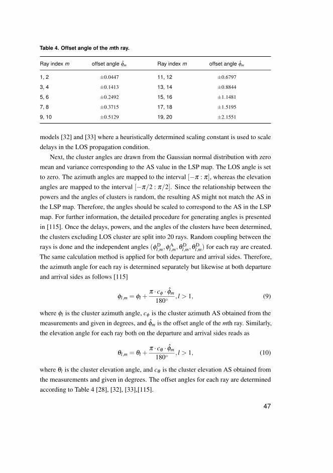
Table 4. Offset angle of the mth ray.

Ray index m offset angle φm Ray index m offset angle φm

1, 2 ±0.0447 11, 12 ±0.6797

3, 4 ±0.1413 13, 14 ±0.8844

5, 6 ±0.2492 15, 16 ±1.1481

7, 8 ±0.3715 17, 18 ±1.5195

9, 10 ±0.5129 19, 20 ±2.1551

models [32] and [33] where a heuristically determined scaling constant is used to scaledelays in the LOS propagation condition.

Next, the cluster angles are drawn from the Gaussian normal distribution with zeromean and variance corresponding to the AS value in the LSP map. The LOS angle is setto zero. The azimuth angles are mapped to the interval [−π : π], whereas the elevationangles are mapped to the interval [−π/2 : π/2]. Since the relationship between thepowers and the angles of clusters is random, the resulting AS might not match the AS inthe LSP map. Therefore, the angles should be scaled to correspond to the AS in the LSPmap. For further information, the detailed procedure for generating angles is presentedin [115]. Once the delays, powers, and the angles of the clusters have been determined,the clusters excluding LOS cluster are split into 20 rays. Random coupling between therays is done and the independent angles (φ D

l,m,φAl,m,θ

Dl,m,θ

Dl,m) for each ray are created.

The same calculation method is applied for both departure and arrival sides. Therefore,the azimuth angle for each ray is determined separately but likewise at both departureand arrival sides as follows [115]

φl,m = φl +π · cφ · φm

180◦, l > 1, (9)

where φl is the cluster azimuth angle, cφ is the cluster azimuth AS obtained from themeasurements and given in degrees, and φm is the offset angle of the mth ray. Similarly,the elevation angle for each ray both on the departure and arrival sides reads as

θl,m = θl +π · cθ · φm

180◦, l > 1, (10)

where θl is the cluster elevation angle, and cθ is the cluster elevation AS obtained fromthe measurements and given in degrees. The offset angles for each ray are determinedaccording to Table 4 [28], [32], [33],[115].

47

In the next step, the polarized channel coefficients are calculated. In the calculationof the polarized channel coefficients, the same XPR value is applied for both verticaland horizontal components. An additional phase offset is added between the horizontaland vertical component of the NLOS rays and the offset angle is calculated to matchthe XPR of circular polarization. The mathematical notations for the calculation ofpolarized channel coefficients are given in [115].

The generic model presented in (2) is then used to determine the channel coefficientfor each cluster. However, a simple summation over 20 rays with random initial phasesdestroys the power information of the cluster. This is fixed by first calculating theaverage power of rays without antenna patterns in each cluster. Then, the scaling factoris obtained from the square root of the ratio between the initial cluster power and theaverage power of rays without antenna patterns. The channel coefficient is determinedby multiplying the channel coefficient obtained from (2) and the scaling factor [115].

Finally, the magnitudes of the channel coefficients are scaled to the correct levelbased on the link distance by using the distance dependent PL and SF. The value of SFis obtained by interpolating the surrounding pixels of the position of the UE in eachsnapshot [115]. Therefore, the path gain including PL and SF is written as [115]

PGt =

√10−PL[dB]

t +SF [dB]t

√1+P1(

KFt

KF1−1), (11)

where SF [dB]t and KFt are the interpolated values of SF and KF at the UE position in

the tth time instant, KF1 is the KF value at the initial position of the UE. In the LOSpropagation condition, the KF has already been included in the scaling of cluster powers.Therefore, the power of the LOS cluster should be scaled accordingly

hnr ,nt ,l(t) = PGt ·

√

KFtKF1·hnr ,nt ,l(t) for l = 1,

hnr ,nt ,l(t) otherwise.(12)

The time evolution of the channel caused by the UE movement, discussed in Section 2.1,is taken into account by updating delays, AoAs, EoAs, and phases for each snapshot ofthe channel within a channel segment. Also, when the UE moves from one segment toanother, the clusters’ birth and death process is modeled as shortly discussed in Section2.1.

48

2.5 Usage of the model

The channel simulations in this thesis are carried out independently for each scenarioand propagation condition. However, the model also supports the simulations ofboth scenarios and propagation conditions in a single simulation run. This meansthat one radio link can be simulated, for instance, under a two-story lobby scenarioLOS propagation condition, whereas another radio link can be simulated for an urbansmall cell scenario NLOS propagation condition. Also, the UE may go through bothpropagation conditions (LOS and NLOS) during its route. This is modeled by thesmooth transition between channel segments. The model also supports variable speedfor the UE including acceleration and de-acceleration of the UE.

The simplest way to use the outcome of this thesis, is to use the PL modelsdetermined at 10 GHz in Section 4.1.1. The validated channel model with the input ofthe determined parameterizations, can also be used for link level and system level studiesat 10 GHz. Since the GSCM can be easily used for simulating different propagationscenarios by selecting the appropriate parameters. The defined parameterizations inChapter 4 can be easily used by adding them as an input of the GCSM. Actually, theparameterizations presented in this thesis have already been utilized in existing research.The model described in this chapter with determined parameterizations has been usedfor creating RF-system requirements for link and system level specifications at 10GHz in [118, 119]. Also, the model parameterizations have been used in system levelsimulations where the co-primary spectrum sharing algorithms have been studied at10 GHz [120]. In addition to the QuaDRiGa channel model, the determined modelparameters are also directly applicable to the WINNER and 3GPP models.

49

3 Experimental radio channel measurements

Channel sounding methods can be categorized several ways, e.g., in terms of waveformor measurement principle. In time domain measurements, channel sounding is based ona pre-known sounding signal at the Tx and Rx. A wideband signal generator is used togenerate a transmitted signal with known sounding sequences such as m-sequences.At the Rx, the incoming signal is then correlated with the known sounding sequence,leading to the channel impulse response (CIR) of the measured channel. The mainbenefit of this method is that even a large MIMO channel can be measured fast byswitching through all the elements of antenna arrays one by one. The main drawbacksof time domain channel sounders are their high cost and limited frequency region.In addition, the synchronization between the Tx and Rx clocks is also a challenge.Although high precision rubidium clocks are used, there might still be some imprecisionin the timing.

Narrowband channel sounding can be performed in a frequency domain with a vectornetwork analyzer (VNA). With this method, the wideband channel can be composedby sweeping continuous wave (CW) signals over the desired bandwidth. The inverseFourier transform of the measured complex frequency response is then calculated toobtain a CIR. VNAs are typically designed for wide frequency bands from some tens ofmegahertz to tens of gigahertz. Therefore, the main benefit of this method is the flexibleselection of the frequency band. On the other hand, the radio frequency (RF)-cablessuffer high losses especially in the higher frequency bands. Because RF-cables of Txand Rx antennas are connected to the same device, this may limit the measurable linkdistance. Typically, this problem is solved either by utilizing RF-optic converters or upand down converting the RF-frequency to an intermediate frequency (IF) band. Withthis method, the MIMO channel can be measured by utilizing virtual arrays. Althoughthe measurement of a single wideband channel is fast, measurement with large antennaarrays might be time-consuming because the antenna elements have to be shifted. Thisis also the drawback of VNA-based MIMO measurements because the channel must bestationary during the measurement from each Tx virtual antenna element to each Rxvirtual antenna element.

In this chapter, experimental channel measurements at 10 GHz are presented.Section 3.1 introduces the measurement equipment and the antennas used in the field

51

measurements. Section 3.2 describes the MIMO channel measurements which werecarried out in order to characterize the 3-D channel in two different propagationenvironments, a two-story lobby and urban small cell at 10 GHz. Section 3.3 discussesthe complementary single-input single-output (SISO) measurements in an outdoor-to-indoor (O2I) propagation scenario. Finally, the post-processing of the measurement datais shortly described and the validation of the estimated MPCs using a semi-deterministicmap-based model is presented in Section 3.4.

3.1 Measurement equipment and antennas

The block diagram of the MIMO radio channel measurement setup is presented inFig. 5. A Keysight N5247A four-port PNA-X [121] was used as a channel soundingdevice in all measurements. For measuring a MIMO radio channel with VNA, virtualarrays [122] were used at the Tx and Rx. In other words, a single antenna elementwas placed in several positions in order to virtually form an antenna array. A dualpolarized patch antenna element [107] was used at the Tx and Rx. The antenna hada half power beamwidth of 125◦ and a maximum gain of 4 dBi over the measuredbandwidth. Two orthogonal polarization planes were slanted to ±45◦ from the verticalplane. The cross-polarization discrimination (XPD) of the antenna element was between18 dB and 22 dB over the operating bandwidth. For further information, the detailedantenna properties are presented in [107].

Controllable antenna positioners (denoted as antenna robots in Fig. 5) consisting ofstepper motors, linear stages, and rotatory table were used to move the antenna elementsin 3-D space. The VNA were controlled by Matlab based measurement control software.Hence, for the polarized radio channel, S-parameters between the Tx/Rx antenna ports,radiating on parallel and orthogonal planes were recorded. External amplifiers, i.e.,low noise amplifiers (LNAs) [123] and power amplifiers (PAs) [124], were used tocompensate for high cable losses between the VNA and the antennas. The amplifiersoperated in a linear region, leading to 23 dBm of effective isotropic radiated power(EIRP) in a single far-field element.

Complementary O2I measurements were performed with a SISO antenna configu-ration since the target was to analyze the path loss in the case where the radio link isblocked by different types of walls. In the SISO measurements, vertically polarized hornand dipole antennas were used as the Tx and Rx antennas, respectively. The gain of theTx antenna was 13 dBi [125] whereas the gain of the Rx antenna was 2.1 dBi. As in

52

Radio Channel

Ethernet

Rx

antenna

Tx

antennaTo move the

antenna

RF-cablesRF-cables

RF-cable

Ethernet

connection

Mechanical

connection

To move the

antenna

PORT 4

PORT 2

PORT 3

PORT 1

PA

PA

LNA

LNA

Fig. 5. A block diagram of the measurement setup for the measuring MIMO channel. ([93]c© 2016 IEEE.)

the MIMO measurements, external amplifiers were used to compensate for high cablelosses between the VNA and the antennas. In all measurements (MIMO and SISO), themeasurement system was calibrated by performing a reference measurement with 60dB attenuators between the PAs and LNAs. Through the calibration procedure, theRF-cables and amplifiers were canceled out from the measured data.

3.2 MIMO measurements

This section describes the performed MIMO radio channel measurements in two-storylobby and urban small cell environments. The aim of the measurements was to derive afull set of 3-D parameters for the GSCM. The recording time for a MIMO channel withVNA and virtual antenna arrays increases significantly in comparison to the traditionaltime domain channel sounders and antenna arrays. The number of virtual antennaelement positions, the dwell time (i.e., the waiting time between measuring each tone),the sweep time of the channel, and IF-bandwidth affect the duration of the measurementand quality of the measurement data. The dwell time must be long enough in order thatall the propagation paths are captured at the Rx before measuring the next tone. Also, anarrower IF-bandwidth gives a higher measurement dynamic range, but on the other

53

hand increases the minimum sweep time. In order to extract the directional informationfrom the propagation channel, the scan time of the antenna arrays, i.e., the time it takesto measure a channel between all Tx-Rx antenna pairs must be shorter than the channelcoherence time. Therefore, a trade-off between the measurement speed, the number ofvirtual antenna element positions, and the measurement settings had to be made. Due tothe long scan time of virtual antenna arrays, the measurements were carried out in astatic environment. Furthermore, the Tx and Rx were fixed during the data recordings.The main measurement settings are presented in Table 5.

Table 5. Measurement settings in MIMO measurements.

Parameter Value

Center frequency 10.1 GHzBandwidth 500 MHzNumber of frequency points 801/401*VNA Rx IF-bandwidth 100 kHzVNA output power 10 dBmTx cable attenuation 19 dBRx cable attenuation 10 dBPA gain 29 dBPA 1 dB compression point 25 dBLNA gain 25 dBLNA noise figure 1.8 dBTransmission power (EIRP) 23 dBmTotal measurable dynamic range 130 dB

* 801 in the two-story lobby and 401 in urban small cell measurements.

At first, the measurements were performed in the two-story lobby environment.In these measurements, the Tx virtual array was capable of measuring only a singledimension. Therefore, a horizontally aligned uniform linear array (ULA) containing ninedual polarized antenna elements was selected. In order to characterize an omnidirectionalchannel at the Rx, the Rx virtual array was a conformal array shaped like a lateralsurface of a cube. Each vertical side had 9×9 planar arrays with dual polarized antennaelements, leading to 324 dual polarized Rx antenna elements. Thus, 2916 (9×9×9×4)dual polarized channels were measured at each measurement spot.

After the measurements in the two-story lobby environment, the measurementsystem was upgraded. With the upgraded measurement setup, the Tx virtual arraywas capable of measuring both vertical and horizontal dimensions. In the urban small

54

cell measurements, the Tx virtual array was 5×5 uniform rectangular array (URA).The shape of the Rx virtual array was the same as in the two-story lobby environment.However, the capability of measuring both vertical and horizontal dimensions at theTx increased the array scan time. Therefore, the number of virtual antenna elementpositions at the Rx were decreased from nine to five in both dimensions. Hence, 2500(5×5×5×5×4) dual polarized channels were measured at each measurement spot.The spacing between each virtual antenna element position was half the wavelength atboth ends of the link in both scenarios. The element positions of the virtual arrays inboth measurement scenarios are illustrated in Fig. 6 and the antenna configurations aresummarized in Table 6. In general, the used measurement system is easily scalable fordifferent MIMO configurations.

0 0.12

0

X [m]

Z [m

]

00.05

0.10.15

00.05

0.10.15

0

0.05

0.1

0.15

Y [m]X [m]

Z [m

]

(a)

-0.02 0 0.02 0.04 0.06 0.08

X [m]

-0.02

0

0.02

0.04

0.06

0.08

Z [m

]

0.1

0

0.1

Z [m

] 0.05

0.05

X [m]

0.05

Y [m]

0.1

0 0

(b)

Fig. 6. Antenna element positions in Tx and Rx virtual arrays in (a) two-story lobby environ-ment ([93] c© 2016 IEEE.) (b) urban small cell.

3.2.1 Two-story lobby environment

The measurements were carried out in a two-story lobby area on the campus at theUniversity of Oulu. Both LOS and NLOS propagation conditions were considered. Aphotograph of the measurement environment in the second floor hallway is displayed inFig. 7. The environment consists of a restaurant area on the first floor, partly open to the

55

Table 6. Antenna configurations in MIMO measurements.

Parameter Two-story lobby Urban small cell

Tx antenna element Dual polarized patch antennaNumber of Tx virtual element positions 9 25Arrangement of Tx virtual elements Horizontal ULA URARx antenna element Dual polarized patch antennaNumber of Rx virtual element positions 324 100Arrangement of Rx virtual elements Planar in each lateral surfaces of a cube

Tx

Rx

Fig. 7. Photograph of the measurement environment in the second-floor hallway. ([93]c© 2016 IEEE.)

second floor and a hallway above the restaurant area on the second floor. Both of thefloors have linoleum flooring, the walls and the ceilings of the surroundings are made ofconcrete and there are several metal fences and offices with walls made of glass. Thefences blocked the LOS propagation in some of the higher elevation measurement pointsfrom the top floor down to the bottom floor. The measurement data was recorded atnight to minimize the scattering from people walking in the environment. The corridorswere not blocked during the measurements, but the effects of solitary moving scattererswere considered negligible because of the very long virtual array scan time.

A floor plan of the measurements is given in Fig. 8. The Tx array positions arepresented as black markers. The positions were selected to represent realistic accesspoint heights on the walls. The selection of measurement points was restricted by the

56

Tx1 0°-direction

Tx2 0°-direction

Tx3 0°-direction

Tx4 0°-direction

Rx1 0°-direction

Rx2 0°-direction

Rx3 0°-direction

Rx4 0°-directionSecond floor hallway

First floor restaurant

Stationery shop

20 30 40 50 60 70 80

X [m]

15

20

25

30

35

Y [m

]Tx1 Tx2 Tx3 Tx4 Rx1 Rx2 Rx3 Rx4

Fig. 8. Floor plan and measurement spots. The same type of Tx and Rx markers designatethe measurements from the Tx array to the Rx array. Filled Rx markers denote Rx arraypositions in the NLOS measurements. The zero directions of the virtual arrays are depictedby the arrows. ([93] c© 2016 IEEE.)

length of the RF-cables. The Rx array positions are presented as blue and red markerswhere the colors refer to the LOS and NLOS propagation conditions, respectively. Atthe Tx, the patch antenna was oriented parallel to the surface of the virtual ULA. TheRx patch antenna was oriented parallel to each vertical surface of the cube. The zerodirections of the virtual arrays are depicted by the black arrows in Fig. 8.

The measurement campaign was divided into four parts, denoted as Tx1–Tx4 andRx1–Rx4 in Fig. 8:

– LOS measurements in the second-floor hallway (Tx1, Rx1);– LOS and NLOS measurements in the first-floor restaurant area (Tx2, Rx2);– LOS and NLOS measurements from the hallway of the second floor to the restaurant

area of the first floor (Tx3, Rx3);– NLOS measurements in the second-floor hallway (Tx4, Rx4).

In addition, 11 Rx array positions close to each other (circles in Fig. 8) in thesecond-floor hallway were recorded in order to obtain meaningful data for correlationdistance analysis. In total, 20 LOS and 13 NLOS measurement spots were measured.The antenna heights of the Rx and Tx were 1.6 m and 2 m, respectively. The height ofthe first floor was 3.2 m. Therefore, in the measurements from the second-floor hallwayto the first-floor restaurant, the Tx antenna height with respect to the first floor was5.2 m. The measurement dynamic range, i.e., the difference between the strongestpropagation path and noise, was more than 40 dB and 20 dB in the LOS and NLOSmeasurements, respectively.

57

3.2.2 Urban small cell

The urban small cell measurements were carried out in two different locations in thecampus area at the University of Oulu. The measurement layouts are illustrated in Fig.9 where the boresights of the Tx arrays are depicted by arrows. As in the two-storylobby environment, both LOS and NLOS propagation conditions were measured and 10snapshots were recorded per antenna element position. In the first measurement location(Fig. 9(a)), the Tx array was located on the staircase and the measurements consisted oftwo different sites. The first site (Tx1, Rx1 LOS) was an alleyway with vegetation onone side. The building walls consisted of a few windows and the surface material ofthe walls was a marble slab. At the second measurement site (Tx2, Rx2 LOS and Rx2NLOS), the propagation environment was an urban street canyon type of environment.The environment consisted of office buildings with surface material of concrete on bothsides of the street canyon. A photograph of the first measurement location is presentedin Fig. 10(a). In the second location (Fig. 9(b)), the measurement environment consistedof five-story office buildings with heights of approximately 15 m. The material of thebuilding walls was a mixture of concrete and corrugated metal facing. A photograph ofthe second measurement location is presented in Fig. 10(b).

The positions of the Tx virtual array were selected to represent a possible locationof a BS and the virtual array was downtilted by 5◦ with respect to the horizon in allmeasurements. The measurement dynamic range was more than 40 dB and 20 dB inall LOS and NLOS measurements, respectively. The height of the Tx antenna wasapproximately 10 m while the height of Rx was 2m. The lengths of the RF-cables were28 m and 10 m to the Tx and Rx, respectively. Therefore, the maximum link distance inthe measurements was around 36.5 m. In total, 21 LOS and 11 NLOS measurementspots were measured.

3.3 Outdoor-to-indoor SISO measurements

In order to characterize the path loss from the outdoor BS to the indoor mobileuser, complementary O2I measurements were carried out. The measurement settingswere adjusted in comparison to the MIMO measurements and the main settings aresummarized in Table 7.

The measurements were carried through two different types of walls: a glass windowand a concrete wall. The Tx and the Rx were immobile during the measurement

58

(a) (b)

Fig. 9. Measurement spots and layouts (a) location 1 (b) location 2. Gray shaded blocksindicate buildings. The same type of Tx and Rx markers designate the measurement fromthe Tx array to the Rx array. Arrows illustrate the boresight of the Tx array.

(a) (b)

Fig. 10. A photograph of the (a) first measurement location (b) second measurement loca-tion.

data recordings. The height of the Rx antenna was 1.3 m in all measurements andthe Tx antenna had three different horizontal positions in both measurements. Themeasurements layouts are illustrated in Fig. 11.

In the measurements through the glass window, the Rx antenna was located in thelobby and the heights of the Tx antenna were 3.8 m, 1.4 m and 1.2 m in all horizontalpositions. The wall between the Tx and the Rx consisted of two layered glass windowswith densely spaced metallic frames as shown in Fig. 12. The lobby was not blockedduring the measurements. However, there were some people moving in the lobby during

59

Table 7. Measurement settings in SISO measurements.

Parameter Value

Center frequency 10.1 GHz

Bandwidth 500 MHz

Number of frequency points 401

VNA Rx IF-bandwidth 10 kHz

VNA output power 14 dBm

Tx cable attenuation 29 dB

Rx cable attenuation 10 dB

Gain of Tx antenna 13 dBi

Gain of Rx antenna 2.1 dBi

Transmission power (EIRP) 27 dBm

(a) (b)

Fig. 11. Top view layouts of the O2I measurements (a) through the glass window (b) throughthe concrete wall. Gray shaded blocks indicate indoor areas. ([95] c© 2016 IEEE.)

the measurements. Photographs of the outdoor Tx antenna and indoor Rx antenna forthe measurements through the glass window are shown in Fig. 12.

For the measurements through the concrete wall, two dipole antennas were used atthe Rx. The separation between the dipole antennas was 40 cm. The purpose of havingtwo Rx antennas was to increase the robustness of the measured path loss. In thesemeasurements, the Rx antenna was located in the empty meeting room where there were

60

(a) (b)

Fig. 12. O2I measurements through the glass window (a) outdoor Tx antenna (b) Rx antennain the lobby. ([95] c© 2016 IEEE.)

(a) (b)

Fig. 13. O2I measurements through the concrete wall, (a) outdoor Tx antenna (b) Rx anten-nas in the meeting room. ([95] c© 2016 IEEE.)

two tables in the middle of the room. The heights of the Tx antenna were 1.3 m and 5.1m. Photographs of the outdoor Tx antenna and indoor Rx antennas in the measurementsthrough the concrete wall are displayed in Fig. 13.

3.4 Post-processing

This section describes the main principles of the post-processing of the measurementdata. A detailed description of the propagation estimation process in general, can befound in the PhD Dissertation of Claudio Ferreira Dias [97]. The propagation pathswere extracted by utilizing estimation of signal parameters by rotational invariance

61

techniques (ESPRIT) [126] due to its reasonable processing time for large antennaconfigurations in comparison to space-alternating generalized expectation-maximization(SAGE) [127], initial and search improved SAGE (ISIS) [128], and RIMAX [129].Before the propagation paths were extracted, the measured frequency domain data wasfiltered in order to prevent frequency leakage. Several windows including Hanning,Hamming, and Kaiser windows were tested for the measured frequency responses. TheKaiser window [130] with a roll-off factor of 5 was selected for the collected data fromthe MIMO measurements.

In the measurements in the two-story lobby environment, the measurement dataconsisted of a five-dimensional (5-D) transfer function (frequency, polarization, theposition of Tx antenna in the horizontal axis, the position of Rx antenna in the horizontaland vertical axes). The noise cutoff level was first set 6 dB above the noise level.Each propagation path was extracted using an inverse fast Fourier transform (IFFT)for the time of arrival (delay), a unitary R-dimensional ESPRIT [131] for angularestimates, and the polarization amplitudes. The R-dimensional ESPRIT implementationfollows the mathematical notations given in [97], [132], [133]. Since the Tx virtualarray was the horizontally aligned ULA, the EoDs of the propagation paths cannot bedirectly estimated. However, once the other directions (AoA and EoA) and delay of thepropagation path were available, a geometric approach [134] was used to determinethe EoDs. In the urban small cell measurements, the upgraded measurement systemalso enabled the estimation of the EoDs. As an output, each propagation path m wascharacterized by a nine-element parameter vector

Θm = [τm,a++m ,a+−m ,a−+m ,a−−m ,φ D

m ,θ Dm ,φ A

m ,θ Am ], (13)

where τm is the delay, a++m ,a+−m ,a−+m , and a−−m are the complex amplitudes of each

polarization component, φ Dm is the AoD, θ D

m is the EoD, φ Am is the AoA, and θ A

m is theEoA. For the different polarization components, superscripts {+,−} designate +45◦

and −45◦ measured polarizations from the vertical plane, respectively. The first and thesecond superscript indicate the received and transmitted polarizations, respectively.

The antenna radiation patterns of the measurement antennas can be de-embeddedby SAGE, ISIS, and RIMAX algorithms. In the case of the ESPRIT algorithm, theradiation patterns of the Tx and Rx antennas must be removed after the estimationprocess. In a virtual array, the antenna element is physically the same and there is nomutual coupling between antenna elements. Hence, single element patterns can beused to cancel the effect of the antennas afterwards. Since the shape of the Rx virtual

62

array was the lateral surface of a cube, the multipath estimation was first made for eachface of the cube independently. The range of detectable paths was limited to a sectorfrom −45◦ to +45◦ for azimuth and from −90◦ to +90◦ for elevation with respectto the broad side. After the estimation, the gain and the angular information of thepropagation paths together with the measured 3-D antenna radiation patterns were usedto cancel the effect of the antennas. Finally, an equivalent omnidirectional propagationchannel seen at the Rx was obtained by joining all faces of the cube. As the last step ofthe post-processing, the complex valued amplitudes of each vertical and horizontalpolarization components aVV

m ,aVHm ,aHV

m , and aHHm were obtained from the estimated

amplitudes of ±45◦ polarization components by applying a Jones matrix [135]

J(ϑ) =

[cos(ϑ) −sin(ϑ)

sin(ϑ) cos(ϑ)

], (14)

where ϑ = −45◦·π180◦ is the rotation angle[

aVVm aVH

m

aHVm aHH

m

]= J(ϑ)

[a++

m a+−m

a−+m a−−m

]J(ϑ)H. (15)

An example of the delays, AoAs, and gains of the estimated propagation pathsin the two-story lobby measurement environment in LOS propagation condition isdisplayed in Fig. 14. In this example, the Tx and Rx arrays were facing each otherand the distance between them was 11.64 m. The LOS component is clearly identifiedand its attenuation follows the free space loss. In addition, a strong NLOS multipathcomponent is observed.

In the O2I SISO measurements, the Kaiser window with a roll-off factor of 8was used. The CIR was then obtained from the frequency response by IFFT. In themeasurements through the concrete wall, each snapshot consists of two CIRs whichwere combined for representing the CIR of the SISO channel as follows

hSISO(τ) = (2

∑nr=1|hnr ,1(τ)|2)/2. (16)

In the analysis of the CIR, there are several methods for determining the noise cut offlevel. A typical method is to determine the noise level from the noise samples of the CIRand set the noise cut off level a few dBs above it [136, 137]. However, in [138], it wasproposed to set the noise cut off level 20 dB below the strongest peak of the CIR. In fact,weak paths have a minimal effect on the path loss. Therefore, this method was used for

63

350300

250200

Delay [ns]

150

-115

-110

-105

100180

-100

135

-95

AoA [deg]

Pro

paga

tion

path

gai

n [d

B]

90

-90

5045

-85

0

-80

-75

-45 -90-135-180-120

-115

-110

-105

-100

-95

-90

-85

-80

-75

Pro

paga

tion

path

gai

n [d

B]

Fig. 14. An example of the delays, AoAs, and gains of the estimated propagation paths inthe two-story lobby LOS scenario. ([93] c© 2016 IEEE.)

the SISO measurement data in this thesis. In order to avoid distinguishing the path lossfrom the paths which are actually noise, CIRs with at least a 23 dB dynamic range (thedifference between the strongest peak and noise level) were accepted for the analysis.The noise threshold was then set to 20 dB below the strongest path of the CIR and thepaths within 20 dB from the strongest path were included in the analysis. Fig. 15 showsan example of the measured CIR and the determination of the noise cut off level.

3.4.1 Validation of the multipath estimation

How can we ensure that the estimated multipaths correspond to the measured propagationenvironment? In general, there are a couple of simple methods to evaluate the qualityand reliability of the estimated propagation paths. One way is to calculate the recoveredenergy ratio between the estimated MPCs before the cancelation of the antenna patternsand raw measured data. Fig. 16 presents a cumulative distribution function (CDF) of therecovered energy ratios in both scenarios and propagation conditions. For the two-storylobby environment, the mean percentages of recovered energy ratios were 87% and

64

0 50 100 150 200 250 300 350 400 450−130

−120

−110

−100

−90

−80

−70

−60

# Path

Pat

h ga

in [d

B]

Channel impulse responsePaths included to the analysisNoise cut off level

Fig. 15. An example of the CIR in O2I SISO measurements through the glass window.

87.5% in LOS and NLOS propagation conditions, respectively. Equivalently, the meanpercentages for the recovered energy ratios were 89.3% and 88.4% for LOS and NLOSpropagation conditions in the urban small cell environment. In order to validate theestimated energy of each delay bin, the DS between the measured raw data and theestimated MPCs before the cancelation of the antenna patterns are presented in Fig. 17.These plots show the agreement between raw and estimated data.

However, the recovered energy ratios and delay spreads do not tell us anything aboutthe directions of the estimated MPCs which have a major impact on the model behavior.An easy method of gaining an initial approximation of the quality of the estimatedmultipath directions is to use the map of the measurement environment and evaluatewhether the directions of the MPCs make sense or not. Although the directions of theMPCs might make sense, the gain of each MPC is difficult to solely evaluate based onthe map of the measurement environment. In order to get a more sophisticated validationof the estimated MPCs, a semi-deterministic map-based model shortly introduced inSection 1.2.2 was used to validate the estimated multipaths.

65

75 80 85 90 95 1000

0.2

0.4

0.6

0.8

1

Recovered energy %

CD

F

LOSNLOS

(a)

75 80 85 90 95 1000

0.2

0.4

0.6

0.8

1

Recovered energy %

CD

F

LOSNLOS

(b)

Fig. 16. Recovered energy ratios for (a) the two-story lobby (b) the urban small cell scenario.

0 10 20 30 40 500

0.2

0.4

0.6

0.8

1

DS [ns]

CD

F

Meas. LOSEstim. LOSMeas. NLOSEstim. NLOS

(a)

0 10 20 30 40 50 600

0.2

0.4

0.6

0.8

1

DS [ns]

CD

F

Meas. LOSEstim. LOSMeas. NLOSEstim. NLOS

(b)

Fig. 17. The DS between raw measurement data and estimated MPCs before the cancelationof the antenna patterns for (a) two-story lobby (b) urban small cell scenario.

66

In the validation of multipaths, a subset of the measurement data in the urban smallcell was used. During the measurements, the dimensions and positions of the walls,other fixed structures, and the Tx & Rx arrays were measured using a laser distancemeter. Based on this information, a 3-D map was defined in the Cartesian coordinatesystem for the modeled environment. The walls of the buildings were modeled asrectangular surfaces with specific electromagnetic material properties. A simplifiedillustration of the measurement layout and the evaluated measurement spots are given inFig. 18.

Fig. 18. Layout of the second measurement location for the urban small cell measurements,subset of measurement spots, and coordinate system of the azimuth angles at both ends ofthe link. Gray shaded blocks indicate buildings. ([96] c© 2016 VDE Verlag/IEEE.)

The propagation paths were modeled deterministically in terms of rays. Thecoordinated system of azimuth angles (AoA and AoD) is given in Fig. 18. The zeroangle points to the East, 90◦ to the North, −90◦ to the South and ±180◦ to the West.The horizon is set as 0◦. Hence, the positive EoD and EoA are the upward direction fromthe horizon, whereas the negative EoD and EoA are downward from the horizon. In themodel, after the Tx and Rx positions were set, all possible secondary nodes visible tothe Tx / Rx node either via the LOS propagation path or via a single specular reflectionwere identified. Possible secondary nodes include diffraction points such as corners,scattering objects or diffuse scattering point sources. Although random objects are part

67

of the map-based model, they were not considered in this case because the measurementenvironment was static during the data recordings. The single specular reflections aremodeled by Fresnel reflection coefficients [139]. In the model, the uniform theoryof diffraction (UTD) is used for modeling diffraction. Besides, the 3-D map of themeasurement environment, a small set of parameters is determined for the model. Theratio between specular reflection and diffuse scattering describes the weighting betweenspecular reflection and diffuse scattering point sources. If the ratio is set to zero, thepaths do not propagate via specular reflection. On the other hand, if the ratio is set tounity, the paths do not propagate via diffuse scattering point sources. In this work, theratio is set to 0.5 as recommended in [16], and a relative permittivity of 5.31 [140] wasused in the modeling of specular reflections from the concrete walls and the diffractionfrom the corners of buildings.

Fig. 19 shows the measured (calculated from the amplitudes of estimated multipaths)and modeled path losses. In addition, the free space loss is included as a reference.Since the LOS propagation path is close to the free space loss, the other propagationpaths give the multipath gain resulting in a lower path loss than the free space loss. Themeasured path losses match the modeled path losses in the LOS case. In the NLOS case,the measured path loss differs from the modeled path loss at the boundaries, i.e., at thelink distance close to 21 m and 27 m. Based on the directions and the delays of themeasured propagation paths at these measurement points, the radio wave is propagatingvia multiple specular reflections which was not modeled in the map-based model.

Figs. 20–21 present the PDP in LOS and NLOS propagation conditions, respectively.In each Rx position, the propagation paths which are 30 dB and 20 dB weaker than thestrongest propagation paths are discarded in the LOS and NLOS cases, respectively. TheRx positions are displayed from the shortest to the longest link distance.

In the LOS case, the delays and gains of the strongest propagation paths are quitesimilar. Some mismatch is seen for the weaker paths. In the modeled PDP, the gains anddelays of the weaker propagation paths are almost similar over all Rx positions. Thesepaths come via diffuse scattering point sources from the vertical wall on the left side ofthe Tx (Fig. 18). From the measured PDP, these paths are not observed at the first threeRx positions. Also, the measured propagation paths with a long delay are substantiallyweaker at the other Rx positions when compared to the modeled paths.

For the first three Rx position in the NLOS case, the diffracted propagation pathhas a similar delay and gain around from −110 dB to −112 dB in the modeled andmeasured PDP. In the remaining Rx positions, the gain of the diffracted path is more

68

16 18 20 22 24 26 28 30 32 3470

75

80

85

90

95

100

Link distance [m]

Pat

h lo

ss [d

B]

Meas. LOSModel LOSMeas. NLOSModel NLOSFree space loss

Fig. 19. Measured and modeled path losses. ([96] c© 2016 VDE Verlag/IEEE.)

50100

150200 2

4

6

8−120

−110

−100

−90

−80

−70

Rx positionDelay [ns]

Pro

paga

tion

path

gai

n [d

B]

(a)

50100

150200 2

4

6

8−120

−110

−100

−90

−80

−70


Pro

paga

tion

path

gai

n [d

B]

(b)

Fig. 20. PDP in the LOS (a) measured (b) modeled. ([96] c© 2016 VDE Verlag/IEEE.)

than 20 dB below the strongest path. Therefore, the diffracted propagation path cannotbe observed in the other Rx positions in Fig. 21. In these Rx positions, the gains of themeasured propagation paths are smoothly distributed over the delay when comparedto the modeled propagation paths. In the modeled PDP, the strongest propagationpath is clearly identified. The reason for the difference is explained by the lack ofdouble specular reflection on the modeled paths and the regularly spaced tiles whichbehave as the source point of diffuse scattering in the model. Furthermore, it should beremembered that the walls in the measurement environment are composed of a mixture

69

50100

150200

250300

2

4

6

8−130

−120

−110

−100

−90


Pro

paga

tion

path

gai

n [d

B]

(a)

50100

150200

250300

2

4

6

8−130

−120

−110

−100

−90


Pro

paga

tion

path

gai

n [d

B]

(b)

Fig. 21. PDP in the NLOS (a) measured (b) modeled. ([96] c© 2016 VDE Verlag/IEEE.)

of concrete and corrugated metal facing which sets a challenge for the modeling ofdiffuse scattering.

In the evaluation of the directions of the propagation paths, the same cut off levelsare used as in the PDP analysis. The stronger paths are presented by larger markers,whereas the weaker paths are presented by smaller markers. Fig. 22 shows the DoD andDoA for the propagation paths between the measured and modeled paths in the fifth Rxposition in the LOS case. This corresponds to the middle Rx position in the LOS caseshown in Fig. 18.

In addition to the direction of LOS propagation path, the propagation path reflectedfrom the ground is found at the same directions in the modeled and measured DoDsand DoAs. A quite strong path is observed at the AoD of −135◦ in the modeled DoD.The same path is observed from the measured DoD but it is some dBs weaker than themodeled path. Some paths have underwent diffuse scattering from the vertical wall onthe left side of the Tx (Fig. 18) and these can be found at the AoA from−180◦ to−135◦

in the modeled DoA. According to the measured DoDs and DoAs, the grid masks on thewalls of buildings in the measurement environment do not act as a strong source ofdiffuse scattering since these paths were not observed from the measured data.

Fig. 23 shows the DoDs and the DoAs between the measured and modeled datain the third Rx position in the NLOS case. This corresponds to the third Rx positionin the NLOS case from the left to the right direction in the measurement layout. Inboth cases (measured and modeled) the diffracted path from the building corner can befound at the AoD close to −60◦, the EoD close to −20◦, the AoA close to 160◦, and theEoA close to 20◦. The gain of the diffracted path is approximately −112 dB in both

70

−180−150−120−90 −60 −30 0 30 60 90 120 150 180

−80

−60

−40

−20

0

20

40

60

80

AoD [Degree]

EoD

[Deg

ree]

Pro

paga

tion

path

gai

n [d

B]

−105

−100

−95

−90

−85

−80

(a)

−180−150−120−90 −60 −30 0 30 60 90 120 150 180

−80

−60

−40

−20

0

20

40

60

80

AoD [Degree]

EoD

[Deg

ree]

Pro

paga

tion

path

gai

n [d

B]

−105

−100

−95

−90

−85

−80

(b)

−180−150−120−90 −60 −30 0 30 60 90 120 150 180

−80

−60

−40

−20

0

20

40

60

80

AoA [Degree]

EoA

[Deg

ree]

Pro

paga

tion

path

gai

n [d

B]

−105

−100

−95

−90

−85

−80

(c)

−180−150−120−90 −60 −30 0 30 60 90 120 150 180

−80

−60

−40

−20

0

20

40

60

80

AoA [Degree]

EoA

[Deg

ree]

Pro

paga

tion

path

gai

n [d

B]

−105

−100

−95

−90

−85

−80

(d)

Fig. 22. Fifth Rx position in the LOS, (a) measured DoDs (b) modeled DoDs (c) measuredDoAs (d) modeled DoAs. ([96] c© 2016 VDE Verlag/IEEE.)

cases. The strongest path has a similar AoD, AoA, and EoA but the EoD differs. In themodeling, this ray undergoes the diffuse scattering from the secondary source pointwhich is somewhat higher than the Tx. According to the measured EoD, the diffusescattering cluster seems to be at the lower height. In the measured DoD, a strong pathis also found at the AoD of −30◦ and the EoD of −20◦. The measured delay of thispath is around 13 m longer than the delay of the strongest path in the model. This rayundergoes a double specular reflection. More precisely, the ray is first reflected from theleft side vertical wall of the middle building. Then, it is reflected from the right-sidewall of the building shown on the left side of the Tx.

Based on the results shown, there is a good match between the dominant estimatedand modeled propagation paths. For weaker propagation paths, some mismatch wasnoticed. However, it is important to notice that the semi-deterministic map-based model

71

−180−150−120−90 −60 −30 0 30 60 90 120 150 180

−80

−60

−40

−20

0

20

40

60

80

AoD [Degree]

EoD

[Deg

ree]

Pro

paga

tion

path

gai

n [d

B]

−112

−110

−108

−106

−104

−102

−100

−98

−96

−94

(a)

−180−150−120−90 −60 −30 0 30 60 90 120 150 180

−80

−60

−40

−20

0

20

40

60

80

AoD [Degree]

EoD

[Deg

ree]

Pro

paga

tion

path

gai

n [d

B]

−112

−110

−108

−106

−104

−102

−100

−98

−96

−94

(b)

−180−150−120−90 −60 −30 0 30 60 90 120 150 180

−80

−60

−40

−20

0

20

40

60

80

AoA [Degree]

EoA

[Deg

ree]

Pro

paga

tion

path

gai

n [d

B]

−112

−110

−108

−106

−104

−102

−100

−98

−96

−94

(c)

−180−150−120−90 −60 −30 0 30 60 90 120 150 180

−80

−60

−40

−20

0

20

40

60

80

AoA [Degree]

EoA

[Deg

ree]

Pro

paga

tion

path

gai

n [d

B]

−112

−110

−108

−106

−104

−102

−100

−98

−96

−94

(d)

Fig. 23. Third Rx position in the NLOS, (a) measured DoDs (b) modeled DoDs (c) measuredDoAs (d) modeled DoAs. ([96] c© 2016 VDE Verlag/IEEE.)

does not aim to be a site-specific prediction tool as RT traditionally does. Therefore, it isconcluded that the estimation accuracy is sufficient.

72

4 Channel model parameterizations

This chapter presents complete 3-D parameterizations for the GSCM described inSections 2.3 and 2.4. The parameters are determined from the channel measurementsdescribed in Chapter 3. In Section 4.1, detailed mathematical descriptions of the analysisitems, i.e., the model parameters are given and a full set of 3-D parameters are derivedfor the GSCM. Section 4.2 shows the path loss model for the O2I propagation scenarioand shortly discusses the frequency dependency of the penetration loss. Finally, themain findings of full 3-D characterization of the propagation channel are summarized inSection 4.3.

4.1 Full 3-D parametrization

The model parameters are extracted by following the methodologies given in theWINNER channel model documentation [114]. In order to analyze the PL, fast-fadingis typically removed from the measurement data by averaging the measurement dataover some tens of wavelengths for the UE movement, e.g., 30 λ0 [141] or 40 λ0 [142].However, in the measurements described in Section 3.2, the Tx and Rx were in fixedpositions. Hence, there is no fast-fading in the measured data. In both scenarios(two-story lobby and urban small cell environments), the parameters are determinedfor LOS and NLOS propagation conditions. In addition, each measured snapshot isanalyzed independently and the majority of the model parameters are given by thespecific distribution with the mean value µ and standard deviation σ .

4.1.1 Path loss and shadow fading

The most important large-scale characteristics of the radio channel are PL and SF.Recently, there has been extensive discussion on path loss modeling methods. Theprediction accuracy, sensitivity and stability of different path loss modeling optionsfor 5G wireless communications have been addressed, e.g., in [66, 74]. Recently,the distance dependence of PL models with weighted fitting has also been proposed[143, 144]. However, the modeling method is still an open issue in 5G wirelesscommunications. Therefore, two different path loss models, which are widely used inthe literature, are determined. The PL is determined as a linear regression line from the

73

basic transmission losses Lb [145] of the measured channel. The basic transmission lossis calculated as [29]

L[1]b =−10log10(

M

∑m=1

Pm), (17)

where M is the number of estimated propagation paths, Pm is the gain of the mthpropagation path determined by a linear combination of the complex valued amplitudesof the co-polarization and cross-polarization components of both polarizations (verticaland horizontal)

Pm = |aVVm |2 + |aVH

m |2 + |aHVm |2 + |aHH

m |2. (18)

It is worth noting that the basic transmission loss is also called the measured PL in theexisting literature, e.g. in [114], [29]. However, measured PL includes SF and the modeldoes not. Hence, the term basic transmission loss is used instead of measured PL toseparate these fundamentally different quantities.

Two different methods are used for modeling the path loss. The floating intercept(FI) model [28] is presented as

PLFI = β +10α log10(dd0

)+10γPL log10(f

1GHz)+σSF,d > d0 (19)

where d0 = 1m is the reference distance, d is the distance between the Tx and Rx, α

is the coefficient showing the dependence of path loss on distance, β is the floatingintercept PL at the reference distance of 1 m, γPL shows the PL dependence on carrierfrequency f in GHz, and σSF is the standard deviation of SF. σSF describes the fluctuationbetween measured basic transmission losses [145] and path loss model. Because themeasurements covered a relatively narrow frequency range, the γPL term is omitted fromthe model. An alternative PL model where the floating intercept PL β is replaced by thefree space loss at 1 m is termed the close-in (CI) free space reference distance path lossmodel. This is presented as [55]

PLCI = 20log10(4π f

c)+10nlog10(

dd0

)+σSF,d > d0 (20)

where n denotes the path loss exponent and c is the speed of light. In both models ((19)and (20)), the σSF is calculated from the deviation between the basic transmission lossesand modeled path losses. Fig. 24 shows the measured basic transmission losses andmodeled path loss with both methods in both scenarios. In addition, the free space lossis included as a reference. The basic transmission losses are mostly below the free spaceloss in the LOS case. This is because the basic transmission loss of the LOS propagation

74

4 5 6 7 8 9 10 20 3060

65

70

75

80

85

90

95

100

Distance [m]

Pat

h lo

ss [d

B]

L

b LOS

LOS CI modelLOS FI modelL

b NLOS

NLOS CI modelNLOS FI modelFree space loss

(a)

15 20 25 30 35 4075

80

85

90

95

100

Distance [m]

Pat

h lo

ss [d

B]

LOS measuredLOS CI modelLOS FI modelNLOS measuredNLOS CI modelNLOS FI modelFree space loss

(b)

Fig. 24. Basic transmission losses and path loss models (a) two-story lobby ([93] c© 2016IEEE) (b) urban small cell scenario.

path equals the free space loss, and the other propagation paths generate multipath gainfor the basic transmission loss. In both scenarios, the results indicate a roughly 10–15dB larger basic transmission loss in the NLOS propagation condition in comparison tothe LOS.

In [113], it was shown that the FI and CI models can be almost identical when thevariety of link distances and the number of data points in the measurements are largeenough. The obtained results in Fig. 24 indicate that there are some differences betweenthe models in the two-story lobby environment and NLOS propagation conditions inthe urban small cell environment. The path loss models and corresponding σSF arepresented in Table 8.

The determined coefficient showing the dependency of path loss on distance α

in LOS propagation conditions in the two-story lobby environment is very small.Furthermore, the difference between α and the path loss exponent n in NLOS conditionsin the urban small cell scenario is significant. As clearly observable from Fig. 24(b)the FI model (dashed line) gives a better match to the measurement data in NLOSpropagation conditions. On the other hand, for short link distances the FI model wouldproduce overly optimistic path loss values. Hence, it is concluded that the FI model ismore appropriate but must be applied only to the distance range present in Table 8. Thedetermined standard deviations for SF are almost the same in each propagation conditionand scenario with both models. Hence, both models can be used for determining the PL,σSF with its correlation distance and cross-correlations with the GSCM.

75

Table 8. Path loss models and shadow fading.

Parameter LOS NLOS

Two-story lobby Urban small cell Two-story lobby Urban small cell

d [m] 5.5–18 15.7–36.5 5–29 20–27.5FI model

α 1.4 2.0 3.3 4.4β [dB] 56.5 53.2 49.3 32.2σSF [dB] 1.4 2.0 2.6 1.4

CI modeln 1.8 2.0 3.0 3.0σSF [dB] 1.5 2.0 2.7 1.5

0 0.5 1 1.50

0.2

0.4

0.6

0.8

1

ASD [log10

(degrees)]

CD

F

Empirical CDFLog−normal CDF

(a)

0.8 1 1.2 1.4 1.60

0.2

0.4

0.6

0.8

1

ESA [log10

(degrees)]

CD

F

Empirical CDFLog−normal CDF

(b)

Fig. 25. Examples of ECDF and theoretical cumulative distribution in LOS propagation con-dition (a) ASD in a two-story lobby scenario (b) ESA in an urban small cell scenario.

4.1.2 Large-scale parameters

As stated in Section 2.3, all LSPs are modeled with a log-normal distribution withspecific mean and standard variation values. The suitability of a log-normal distributionfor the measured LSPs is shortly investigated by using the Kolmogorov-Smirnov (K-S)goodness-of-fit test [146]. In the K-S test, an empirical cumulative distribution function(ECDF) is tested with respect to the assumed distribution. The K-S test statistics aremeasured between the largest vertical difference between the ECDF and the theoreticalcumulative distribution of the distribution that is being tested. Examples of the ECDFand theoretical cumulative distribution in LOS propagation conditions are shown in Fig.25.

76

The null hypothesis H0 indicates whether the ECDF follows the theoretical distribu-tion or not. The null hypothesis is approved, i.e., the measured and theoretical samplesare from the same distribution, if K-S test statistic D is smaller than the critical value(CV) obtained from the table, e.g., in [147]. The K-S test is applied for DS and anglespreads in LOS propagation condition in both scenarios by utilizing Matlab’s built-inK-S test function. The function returns zero for a null hypothesis H0 = 0 if the samplesare from the same distribution. Typically, the significance level is established in therange from 0.01 to 0.1. The significance level has an impact on the critical value. Thecritical value decreases resulting in a tighter limit for approving the null hypothesis asthe significance level increases. With a significance level of 0.05, the null hypothesis isrejected in part of the angle spread distribution tests in the urban small cell scenario.This is probably caused by the somewhat insufficient amount of collected measurementdata for the statistical test. However, with a significance level of 0.01 the null hypothesisis approved in all tested cases and the results are provided in Table 9.

Table 9. Results of the K-S test in LOS propagation conditions.

Parameter Two-story lobby Urban small cell

H0 D CV H0 D CV

DS 0 0.0849

0.1187

0 0.0630

0.1114ASD 0 0.0935 0 0.1101ASA 0 0.0717 0 0.1063ESD 0 0.0781 0 0.1060ESA 0 0.0689 0 0.0961

In order to verify that the channel model produces the same statistics as the measuredLSPs, the simulated LSPs are added as dashed lines to the remaining figures shownin this section. In other words, the simulated curves correspond to the theoretical(log-normal distributed) curves determined by the mean and standard deviation fromthe measurement data. The simulated curves are obtained by channel simulations (seeSection 5.2) with the parameters presented in Tables 8 and 10–14. The QuaDRiGachannel model implementation [46] is used in the simulations.

Fig. 26 displays the CDF of measured and simulated SFs in both scenarios andpropagation conditions. In this figure, negative SF values indicate a larger overall PL incomparison to a median PL (PL without shadowing term in (20)), whereas positive SFvalues indicate a smaller overall PL in comparison to a median PL. Although, some

77

−10 −5 0 5 10 150

0.2

0.4

0.6

0.8

1

SF [dB]

CD

F

Meas. LOSSim. LOSMeas. NLOSSim. NLOS

(a)

−10 −5 0 5 100

0.2

0.4

0.6

0.8

1

SF [dB]

CD

F


(b)

Fig. 26. Measured and simulated CDFs of SF for (a) a two-story lobby (b) an urban small cell.

differences can be noted between the theoretical (simulated) and the measured curves,the SF can be determined as a log-normal distribution with a zero mean and σSF.

Due to the multipath propagation, the same signal arrives at the Rx via severalpropagation paths each having a different gain, delay and direction. The DS describesthe delay dispersion of the propagation paths. It is calculated according to [148]

DS =

√∑

Mm=1 Pmτ2

m

∑Mm=1 Pm

− τ20 , (21)

where τ0 is the mean excess delay calculated as [148]

τ0 =∑

Mm=1 Pmτm

∑Mm=1 Pm

. (22)

Fig. 27 shows the CDF for measured and simulated DSs in both propagation conditionsand scenarios. In the two-story lobby environment, the measured mean value of the DSis 17.4 ns and 30.4 ns for the LOS and NLOS cases, respectively. Equivalently, themeasured mean values of the DS are 21.45 ns and 41.29 ns for the LOS and NLOS inthe urban small cell environment, respectively. The DS tends to decrease as the carrierfrequency increases due to the higher attenuation of multipath components in some ofthe published results. For instance, the mean DS values are given for the frequencybands 10–70 GHz in [71]. These results show that as the carrier frequency increases theDS decreases. In contrast, the frequency dependency of the DS has not been observedin [52] where for example the measured mean value of the DS is given for the urbanmicrocell scenario at the frequency bands 14.8–73 GHz. In general, the DS is very

78

0 20 40 60 80 1000

0.2

0.4

0.6

0.8

1

DS [ns]

CD

F


(a)

0 20 40 60 80 1000

0.2

0.4

0.6

0.8

1

DS [ns]

CD

F


(b)

Fig. 27. Measured and simulated CDFs of DS in (a) two-story lobby ([93] c© 2016 IEEE) (b)urban small cell.

sensitive to the dynamic range in the measurements. If the dynamic range is low, e.g.,below 20 dB, the multipath components arriving with long delay might disappear intothe system noise resulting in a small DS.

The KF describes the ratio between the gains of the LOS propagation path and otherpropagation paths. In general, the larger the KF, the more dominant the LOS propagationpath is. There are at least two different methods for determining the KF. The simplermethod is to calculate the KF as the power ratio between the LOS propagation path andall other estimated propagation paths [148]. An alternative method is to calculate the KFby using the moment-method [149]. In the moment-method, the KF is determined overcertain wavelengths of Tx or Rx movement, i.e., an average over an SSF area, e.g., 30λ0 (cf. Section 4.1). However, the moment-method cannot be used for determiningthe KF from the measured data because the Tx and Rx were in fixed positions duringthe measurement data recordings, i.e., there is no fast-fading in the measurement data.Therefore, the KF is calculated as

KF =PLOS

∑m6=LOS Pm, (23)

where PLOS is the gain of LOS propagation path4. Fig. 28 presents the CDFs for themeasured and simulated KFs in LOS propagation conditions. The mean values of themeasured KFs are 8.5 dB and 5.1 dB for the two-story lobby and urban small cell

4It is worth noting that the impact of the energy that was not detected in the estimation affects the gains of theMPCs. Therefore, with a perfect estimator (100% recovered energy), the KF would be probably smaller.

79

−5 0 5 10 15 200

0.2

0.4

0.6

0.8

1

KF [dB]

CD

F

Meas.Sim.

(a)

−5 0 5 10 150

0.2

0.4

0.6

0.8

1

KF [dB]

CD

F

Meas.Sim.

(b)

Fig. 28. Measured and simulated CDFs of the KF in LOS for (a) a two-story lobby environment(b) an urban small cell environment.

environments, respectively. The KF in the urban small cell environment is substantiallysmaller in comparison to the lower frequency bands, e.g., in [28], and recently publishedat the higher frequency bands [71], [78]. A possible reason for the smaller KF in theurban small cell scenario are the multiple specular reflections from the concrete wallswhich maintain the energy of the multipath component. However, it should be noted thatthe method for determining KF has not been given in [71], [78] which might have animpact on the results.

The circular AS describes dispersion of the propagation paths due to the multipathpropagation in the angular domain. The AS is calculated according to the specificationof the 3GPP SCM [31]. The AS is calculated utilizing angular estimates, i.e., AoAs,AoDs, EoAs and EoDs, and propagation path gains in

AS = min∆

σAS(∆) =

√∑

Mm=1(ψm,µ(∆))2Pm

∑Mm=1 Pm

, (24)

where

ψm,µ(∆) =

ϕ +2ϖ , if ϕ <−ϖ

ϕ, if |ϕ| ≤ ϖ

ϕ−2ϖ , if ϕ > ϖ

, (25)

where ϖ = π for AoDs and AoAs (ϖ = π/2 for EoDs and EoAs), ϕ = ψm(∆)−µψ(∆)

and

µψ(∆) =∑

Mm=1 ψm(∆)Pm

∑Mm=1 Pm

, (26)

80

where ∆ designates a discrete angle shift from −ϖ to ϖ and

ψm(∆) =

(ψm +∆)+2ϕ, if (ψm +∆)<−ϖ

(ψm +∆), if |(ψm +∆)| ≤ ϖ

(ψm +∆)−2ϕ, if (ψm +∆)> ϖ

. (27)

CDFs for ASs in two-story lobby and urban small cell environments are presentedin Figs. 29–30. In the two-story lobby environment, the simulated angle spreadsfollow the measured angle spreads in the NLOS case. In the LOS case, some mismatchbetween the simulated and measured ASA and ESA can be seen. However, the medianvalues of the ASA and ESA intersect each other. Excluding the ASD in the LOSpropagation condition the simulated ASs follow the measured ASs in the urban smallcell environment. In both scenarios, the contribution of the LOS propagation path isclearly the strongest in comparison to the other propagation paths, leading to smallerazimuth ASs in the LOS case.

In two-story lobby environment, the ESD is larger in the LOS case than in the NLOScase. This is caused by the following two facts. In part of the NLOS measurements,the Rx was located on the first floor, whereas the Tx was located on the second floorcausing a narrow spread of the EoDs. Moreover, the geometrical approach used inthe determination of the EoD is based on a single-bounce model, i.e., the transmittedsignal can only undergo interaction, single specular reflection or diffuse scattering, fromthe surface. Therefore, the ESD parameters in a two-story lobby scenario should beinterpreted carefully. Table 10 summarizes the proposed LSPs of the model.

4.1.3 Cross-correlation parameters

In order to create reliable correlations between radio links in the system level simulations,the LSPs have to be generated with correlation properties [28]. The cross-correlationcoefficient between LSP x and y describes the mutual dependency of the LSPs, i.e.,second order characteristics [114]. Cross-correlation coefficient is defined as follows

ρx,y =∑

Ni=1(x(i)− xµ)(y(i)− yµ)√

∑Ni=1(x(i)− xµ)2 ∑

Ni=1(y(i)− yµ)2

, (28)

where N is the number of measured snapshots, xµ and yµ are the sample means of x andy, respectively. The cross-correlation coefficient is determined as a value from -1 to1. The coefficient is zero if there is no correlation between parameters x and y. If the

81

0 10 20 30 40 500

0.2

0.4

0.6

0.8

1

ASD [degrees]

CD

F


(a)

0 20 40 60 80 1000

0.2

0.4

0.6

0.8

1

ASA [degrees]

CD

F


(b)

0 10 20 30 400

0.2

0.4

0.6

0.8

1

ESD [degrees]

CD

F


(c)

0 5 10 15 20 25 300

0.2

0.4

0.6

0.8

1

ESA [degrees]

CD

F


(d)

Fig. 29. Two-story lobby environment, CDF of (a) ASD ([93] c© 2016 IEEE) (b) ASA ([93]c© 2016 IEEE) (c) ESD (d) ESA ([93] c© 2016 IEEE).

coefficient is positive, both x and y increase or decrease simultaneously. A negativecoefficient indicates that if parameter x increases, parameter y decreases or vice versa.The cross-correlation coefficients are presented in Table 11. In both scenarios, thereis a strong dependency between certain parameters and some of the parameters arealmost fully uncorrelated. In the two-story lobby environment, e.g., there is a strongdependency between the ASD and the DS in both propagation conditions whereas nosignificant correlation can be observed between the KF and other LSPs. In the urbansmall cell environment, the ESD and DS and the ASD and DS have a strong dependencyon each other in the LOS and NLOS propagation conditions, respectively. Equivalently,there is no correlation or the correlation is very small, e.g., between the ASD andASA and the ESA and SF in the LOS case in the urban small cell environment. The

82

0 10 20 30 40 50 600

0.2

0.4

0.6

0.8

1

ASD [degrees]

CD

F


(a)

0 20 40 60 80 100 1200

0.2

0.4

0.6

0.8

1

ASA [degrees]

CD

F


(b)

0 5 10 15 20 250

0.2

0.4

0.6

0.8

1

ESD [degrees]

CD

F


(c)

0 10 20 30 400

0.2

0.4

0.6

0.8

1

ESA [degrees]

CD

F


(d)

Fig. 30. Urban small cell environment, CDF of (a) ASD (b) ASA (c) ESD (d) ESA.

cross-correlation coefficients are sometimes given to one decimal place as in the 3GPPmodels in [32], [33]. However, the cross-correlation coefficients presented in Table 11indicate that the cross-correlation matrix is not positively definite if the coefficients aregiven to only one decimal place (rounded to the closest first decimal) in urban small cellNLOS propagation conditions. Therefore, in order to ensure the cross-correlation matrixis positive definite, the coefficients are given to two decimal places. Since two differentPL models are used, two different SFs are also determined. Hence, two values aregiven as cross-correlation coefficients between SF and other LSPs. The first coefficientdesignates the cross-correlation coefficient determined based on the SF obtained by theFI PL model, whereas the second coefficient is based on the SF obtained by the CI PL

83

Table 10. Large-scale parameters.

Parameter LOS NLOS

Two-storylobby

Urbansmall cell

Two-storylobby

Urbansmall cell

DS log10([s])µDS −7.78 −7.70 −7.55 −7.41σDS 0.13 0.16 0.17 0.14

KF [dB]µKF 8.5 5.1 N/A N/AσKF 3.5 3.2 N/A N/A

ASD log10([◦])

µASD 0.86 1.08 1.32 1.24σASD 0.23 0.35 0.23 0.32

ASA log10([◦])

µASA 1.44 1.47 1.64 1.77σASA 0.11 0.20 0.18 0.08

ESD log10([◦])

µESD 0.91 0.80 0.54 0.89σESD 0.31 0.17 0.49 0.07

ESA log10([◦])

µESA 0.61 1.12 0.82 1.08σESA 0.17 0.10 0.29 0.13

model. In urban small cell LOS propagation conditions the cross-correlation coefficientsbetween the SF and the other LSPs are essentially the same with both PL models.

4.1.4 Correlation distances

The correlation distance describes how long the channel can be assumed to be stationaryfor a certain LSP. As mentioned in Section 2.4, the correlation distance determinesthe length of the channel segment in the correlated LSP map. It is calculated from theautocorrelation function and determined as follows

A(δ ) = E[ξ (d) ·ξ (d +∆d)], (29)

where E[·] denotes the expected value of the argument, ξ is the evaluated LSP and ∆d isthe change of link distance. The value for the correlation distance is determined by theintercept point of the correlation curve and a function y = e−1, where e is the Napier’sconstant [150]. In the two-story lobby environment, the correlation distances are

84

Table 11. Cross-correlations.

LOS NLOS

Two-story lobby Urban small cell Two-story Urban small cell

ASD vs DS 0.77 0.59 0.74 0.82ASA vs DS 0.40 0.58 −0.37 −0.35ASA vs SF 0.38/0.45 0.70 0.55/0.44 0.04/0.32ASD vs SF 0.03/0.10 −0.04 0/0.12 −0.18/−0.38DS vs SF 0.06/−0.02 0.56 0.31/0.46 0.10/−0.21ASD vs ASA 0.72 0 −0.60 −0.20ASD vs KF −0.11 −0.40 N/A N/AASA vs KF −0.07 −0.51 N/A N/ADS vs KF 0.02 −0.44 N/A N/ASF vs KF 0.11/0.11 −0.29 N/A N/AESD vs SF 0.20/0.12 0.67 0.13/0.01 0.26/0.17ESA vs SF 0.19/0.35 −0.04 0.01/−0.15 0.39/0.50ESD vs KF 0.19 −0.43 N/A N/AESA vs KF 0.16 −0.51 N/A N/AESD vs DS 0.27 0.81 −0.64 0.41ESA vs DS −0.17 0.33 −0.73 −0.42ESD vs ASD 0.03 0.54 −0.69 0.31ESA vs ASD 0.15 0.42 −0.64 −0.72ESD vs ASA −0.12 0.58 0.68 0.43ESA vs ASA 0.29 0.29 0.34 −0.03ESD vs ESA −0.04 0.36 0.60 −0.26

determined from the Tx and Rx array positions on the second-floor hallway. In the LOScase, the correlation distances are determined from the closely located Rx array positions(marked as circles in Fig. 8). These measurements were performed with approximately30 cm change in link distance, giving an appropriate grid for the correlation distanceanalysis. In the NLOS case, the correlation distances are approximated since the smallestlink distance change was in order of 2 m. In the approximation, we use the methodpresented in [48]. The correlation for all LSPs in the NLOS case is under 1/e(≈ 0.37)when the change of distance is over 2 m. Therefore, the correlation distance is specifiedas 2 m if the correlation is over 1/e at a link distance change of 1.5 m. If the correlationis between 1/2e(≈ 0.18) and 1/e, a correlation distance of 1 m is proposed.

In the urban small cell environment, the correlation distances are determined fromthe subset of the measurements. More precisely, the correlation distances are determinedfrom the closely located Rx positions at the second measurement location marked

85

as squares in Fig. 9(b). These measurements were performed with link distances inapproximately 1 m increments. The correlation distances are presented in Table 12. Thecorrelation distances for the SF are the same with both PL models in both scenariosand propagation conditions. Correlation distances are shorter in both scenarios incomparison to corresponding parameters given for the lower frequency bands, e.g. in[32]. In the urban small cell environment, the correlation distances are the same in bothscenarios (3 m). These correlation distances are similar in comparison to [71] excludingthe correlation distances for the SF and KF in the LOS case. However, it should benoted that based on our measurements we can only approximate the correlation distance.Moreover, the number of measurement points and the range of the link distances aresomewhat limited for an accurate correlation distance analysis. In order to determinemore accurate correlation distances, a substantially larger amount of measurement datawith continuous data recording and mobile movement would be needed.

Table 12. Correlation distances in meters.

Parameter LOS NLOS

Two-story lobby Urban small cell Two-story lobby Urban small cell

DS 1.5 3 1 3ASD 1.2 3 1 3ASA 1.8 3 2 3SF 1.5 3 2 3KF 1.2 3 N/A N/AESA 1.5 3 2 3ESD 1.8 3 2 3

4.1.5 XPR, PDP, and the delay proportionality factor

The XPR is defined as the ratio of the power received at the same and at the orthogonalpolarization with respect to the transmitted power [114]5

XPRV =∑

Mm=1 |aVV

m |2

∑Mm=1 |aHV

m |2,XPRH =

∑Mm=1 |aHH

m |2

∑Mm=1 |aVH

m |2. (30)

The CDFs of the XPRs in both propagation scenarios are displayed in Fig. 31. In thetwo-story lobby environment, the XPRV is approximately 7 dB higher than the XPRH in5In the LOS propagation condition, the LOS path is not taken into account in the XPR calculations since theLOS path has infinite XPR.

86

both propagation conditions. The physical explanation for this difference may lie inthe fact that there are more vertical surfaces than horizontal ones in the measurementenvironment. Hence, the reflected signal energy for the vertical polarization componenttends to be larger than that of the horizontal polarization [151]. Additionally, in theurban small cell scenario, the XPR for vertical transmission polarization is around 5 dBhigher under both propagation conditions. However, it should be pointed out that theenergy of the reflected signal is heavily dependent on the roughness and electromagneticproperties of the surface, i.e., magnetic permeability, electric permittivity, and electricalconductivity. The XPR parameters of the model are determined as the mean value andthe standard deviation over all XPR values, i.e., XPRV and XPRH . This means that thesame XPR values are used in both vertical and horizontal channels. Therefore, it is notmeaningful to add theoretical curves to Fig. 31.

−5 0 5 10 15 20 25 300

0.2

0.4

0.6

0.8

1

XPR [dB]

CD

F

XPRV LOS

XPRH

LOS

XPRV NLOS

XPRH

NLOS

(a)

−5 0 5 10 15 20 25 300

0.2

0.4

0.6

0.8

1

XPR [dB]

CD

F

XPRV LOS

XPRH

LOS

XPRV NLOS

XPRH

NLOS

(b)

Fig. 31. CDFs of XPR in (a) a two-story lobby ([93] c© 2016 IEEE) (b) an urban small cell.

Since a single slope exponential distribution is used to generate the PDP in themodel (cf. Section 2.4), it is essential to look at the measured PDPs as well. Eventhough the theoretical (simulated) DS curves match the measured ones, they do not tellus everything about the delay distribution and PDP of the channel. In other words, thesame DS can be achieved with different PDPs. The measured PDP is fitted to a singleslope exponential distribution as follows

PDP = exp(−b · τe), (31)

where τe is the excess delay and b is the time constant [114]. Figs. 32–33 present themeasured PDPs in the two-story lobby and urban small cell environments, respectively.

87

Based on these results it can be seen that there is some mismatch between the measuredPDP and the exponential fit particularly in the two-story lobby LOS scenario. In thisscenario, strong MPCs were mainly observed with a very short excess delay and on theother hand with an excess delay of around 65 ns in comparison to the LOS peak, leadingto a poor single slope exponential fit. In the NLOS case, a multi-cluster model presentedin the Saleh-Valenzuela model [35] might have been worth testing. However, becausethe validation results that will be shown in the following chapter show good agreementbetween the modeled channel with a single slope exponential function and the measuredchannel, alternative distributions are not tested for the PDPs.

0 20 40 60 80 100 120

Excess delay [ns]

-35

-30

-25

-20

-15

-10

-5

0

Rel

ativ

e pa

th g

ain

[dB

]

b= 88 MHz

Measured PDPExponential fit

(a)

0 20 40 60 80 100 120

Excess delay [ns]

-20

-15

-10

-5

0

Rel

ativ

e pa

th g

ain

[dB

]

b= 41 MHz


(b)

Fig. 32. Typical PDP in a two-story lobby scenario (a) LOS (b) NLOS.

88

0 20 40 60 80 100 120

Excess delay [ns]

-40

-30

-20

-10

0R

elat

ive

path

gai

n [d

B]

b= 113 MHz


(a)

0 20 40 60 80 100 120

Excess delay [ns]

-25

-20

-15

-10

-5

0

Rel

ativ

e pa

th g

ain

[dB

]

b= 51 MHz


(b)

Fig. 33. Typical PDP in an urban small cell scenario (a) LOS (b) NLOS.

0 2 4 6 80

0.2

0.4

0.6

0.8

1

Delay proportionality factor for DS

CD

F

LOSNLOS

(a)

1 2 3 4 5 60

0.2

0.4

0.6

0.8

1

Delay proportionality factor for DS

CD

F

LOSNLOS

(b)

Fig. 34. Delay proportionality factor for DS a) a two-story lobby (b) an urban small cell.

The generation of the PDP in the model also requires the delay proportionality factorparameter which is used to scale cluster delays. The delay proportionality factor is alsocalled the delay scaling factor, e.g., in 3GPP models [32], [33]. It is determined as theratio between the standard deviation of propagation path delays τm and the DS. TheCDFs of the delay proportionality factor are shown in Fig. 34. The larger DS underNLOS propagation conditions leads to a smaller delay proportionality factor for NLOSin both scenarios. The mean value of the delay proportionality factor is proposed for themodel. Table 13 summarizes the XPR and delay proportionality factor of the model. Inaddition, the XPR is presented separately for XPRV and XPRH .

89

Table 13. Summary of XPR and delay proportionality factor parameters.

Parameter LOS NLOS

Two-storylobby

Urbansmall cell

Two-storylobby

Urbansmall cell

XPR [dB]µXPR 13.7 12.4 9.4 8.2σXPR 5.0 3.8 4.7 7.2

XPRV [dB]µXPRV 17.1 14.7 13.3 10.2σXPRV 2.9 2.3 1.5 4.8

XPRH [dB]µXPRH 10.3 10.1 5.4 6.2σXPRH 4.4 3.6 3.4 2.9

Delay scaling parameter rτ 4.0 3.1 3.2 1.8

4.1.6 Cluster parameters

In this thesis two different frameworks for clustering are used. These frameworks aredescribed in detail in [152]. Even though the clustering algorithm was described for 3-Dmeasurement data in [152], the results were presented only for 2-D measurement data,i.e., excluding the elevation domain. In this thesis, the clustering is performed in 3-D.In both cases, the KPowerMeans clustering algorithm [153] is utilized for groupingpropagation paths to the clusters. For every propagation path, a suitable cluster isdetermined so that the total sum of differences between the propagation paths and thecluster centroids is minimized. The multipath component distance (MCD) [154] withweighted path gains is used as a basic distance metric between each propagation path andpossible centroids. It is worth noting that the presented MCD metric in [154] assumes aspherical coordinated system, i.e., the zero elevation angle corresponds to the inclination,while the horizon and nadir have elevation angles of +90◦ and +180◦, respectively.However, the elevation angles are estimated based on the geographical coordinatedsystem in this thesis. This means that the zero-elevation angle points to the horizonand the inclination and nadir have the elevation angles of 90◦ and −90◦, respectively.Therefore, in order to use the presented MCD metric in [154], the elevation anglesare shifted to a spherical coordinated system. The difference between the frameworksis in the selection of the optimal number of clusters. In the following, the clusteringframeworks are shortly described.

90

In the two-story lobby scenario, the clustering algorithm consists of two phases: 1)initial guess and 2) the KPowerMeans algorithm. In the initial guess phase, the algorithmsets the cluster centroids as described in [152]. Propagation paths within each clusterare determined based on the shortest distance. In the initial guess phase, the numberof clusters Nc is selected based on a cluster gain limit of 0.01. This means that eachcluster should contain at least 1% of the total channel gain. In other words, if the gain ofthe cluster is less than 1% of the total channel gain, it is discarded and the previouscombination of clusters, Nc− 1 clusters is given as the input to the KPowerMeansalgorithm. If the number of clusters in the initial guess and KPowerMeans algorithmdoes not match, a new initial guess is made and the KPowerMeans algorithm is repeated.

For the urban small cell scenario, the KPowerMeans algorithm is executed over thesearch interval of the clusters. The search interval for the number of cluster is set from 2to 20 clusters. In other words, the propagation paths are grouped into two clusters, thenthree clusters, and so forth. Several validation indices, e.g., Caliñski-Harabasz [155],Davies-Bouldin [156], Xie-Beni [157], and Kim-Parks [158], have been proposed fordetermining the optimal number of clusters in existing studies. A combination of theCaliñski-Harabasz and Davies-Bouldin validation indices have shown robust results inthe past [153]. Also, this metric has been recently used, e.g., in [61],[159], and [160].Therefore, it is chosen as the decision metric for the optimal number of clusters.

Examples of identified clusters and the illustration of their physical locations basedon angles and delays in the LOS and NLOS measurements in the urban small cellenvironment are shown in Figs. 35–36. In addition to the direct LOS path and clusterconsisting of ground reflected paths, two single-bounce clusters and four multi-bounceclusters (either double- or triple-bounce clusters) are observed in the LOS example. Thegains of the clusters decrease rapidly as the delays of the paths in the cluster and thenumber of bounces increase. In the NLOS case, the strongest cluster is observed viaa single-bounce cluster. The cluster angle spreads are calculated by (24)–(27) fromthe propagation paths within each cluster. A per cluster shadowing standard deviationdescribes the deviation of powers between the clusters. It can be calculated in twodifferent ways. If the propagation path angles are not available, it can be calculated fromthe delays and gains of the propagation paths. In this case, the clusters are detected fromthe time variant power delay profile and deviations are calculated with respect to thepower delay profile. If all the angular estimates are available, an alternative methodis used. The gain of each cluster is first determined by summing up the gain of eachpropagation path within each cluster. Then, the cluster shadowing standard deviation is

91

5090

100

60 180

150

Del

ay [n

s]

30 120

200

AoD [deg]

0 60

AoA [deg]

250

0 -30-60 -60 -120

-90 -180

(a)

(b)

Fig. 35. Urban small cell LOS scenario, an example of (a) identified clusters (b) physicallocations of clusters.

determined from the standard deviation of the cluster gains [114]. The CDFs of theclustering statistics are shown in Figs. 37–38. The cluster parameters of the model aredetermined from the median values of the results. The median values are rounded to theclosest integers. The proposed cluster parameters of the model are summarized in Table14.

92

5090

100

60

150

180

Del

ay [n

s]

30

200

120

AoD [deg]

250

0 60

AoA [deg]

300

0 -30-60 -60 -120

-90 -180

(a)

(b)

Fig. 36. Urban small cell NLOS scenario, an example of (a) identified clusters (b) physicallocations of clusters.

4.2 O2I path loss model

From the SISO channel, the measured basic transmission loss6 is calculated as [28]

L[2]b =−10log10(

Ns

∑τ=1|h1,1(τ)|2)+GT +GR, (32)

6Since the directions of MPCs cannot be estimated from the SISO channel, the nominal gains of the antennasare used to cancel antenna effects.

93

Table 14. Cluster parameters.

Parameter LOS NLOS

Two-storylobby

Urbansmall cell

Two-storylobby

Urbansmall cell

Number of clusters 6 8 11 10Cluster ASD [◦] 4 3 4 7Cluster ASA [◦] 5 5 4 8Cluster ESD [◦] 2 3 1 5Cluster ESA [◦] 2 3 1 7Per cluster shadowing std ζ [dB] 6 6 4 3

where h1,1(τ) is the channel coefficient for the path delayed by τ , Ns is the number ofCIR samples included in the analysis and GT and GR are the nominal antenna gains atthe Tx and the Rx, respectively. The COST 231 O2I path loss model [42] is used as abaseline in the path loss model creation. This model was also used as an origin in theWINNER [28], IMT-A [34], and 3GPP [32], [33] PL models in O2I scenarios. The PLfrom the outdoor Tx to the indoor Rx consist of outdoor PLout, through-wall PLtw, andindoor PLin path losses

PLO2I = PLout +PLtw +PLin. (33)

The outdoor propagation part is modeled as free space loss for the distance between theTx and the Rx

PLout = LF =−27.55+20log10(dout +din)+20log10( fMHz), (34)

where fMHz is the carrier frequency in MHz, dout and din are the distances in meters fromthe Tx to the wall penetration point and from the external wall to the Rx, respectively.

The through the wall path loss depends on the grazing angle of the external wall θG

PLtw =We +WGe(1−d⊥dout

)2 =We +WGe(1− sin(θG))2, (35)

where d⊥ is the perpendicular distance from the Tx to the external wall and We is theexternal wall penetration loss at the perpendicular grazing angle. WGe is the additionalloss on the external wall due to θG 6= 90 degrees. Since there are no internal wallsbetween the external wall and the indoor Rx, the indoor propagation excess loss ismodeled as [161]

PLin = αindin, (36)

where αin in dB/m is the indoor propagation loss coefficient.

94

0 10 20 30 40 500

0.2

0.4

0.6

0.8

1

Cluster ASD [degrees]

CD

F

LOSNLOS

(a)

0 10 20 30 40 500

0.2

0.4

0.6

0.8

1

Cluster ASA [degrees]

CD

F

LOSNLOS

(b)

0 10 20 30 400

0.2

0.4

0.6

0.8

1

Cluster ESD [degrees]

CD

F

LOSNLOS

(c)

0 5 10 15 20 25 300

0.2

0.4

0.6

0.8

1

Cluster ESA [degrees]

CD

F

LOSNLOS

(d)

0 5 10 15 200

0.2

0.4

0.6

0.8

1

Number of clusters

CD

F

LOSNLOS

(e)

0 2 4 6 80

0.2

0.4

0.6

0.8

1

Per cluster shadowing std [dB]

CD

F

LOSNLOS

(f)

Fig. 37. Two-story lobby scenario, CDF of (a) cluster ASD ([93] c© IEEE) (b) cluster ASA ([93]c© IEEE) (c) cluster ESD (d) cluster ESA ([93] c© IEEE) (e) number of cluster (f) per clustershadowing standard deviation.

95

0 10 20 30 40 500

0.2

0.4

0.6

0.8

1

Cluster ASD [degrees]

CD

F

LOSNLOS

(a)

0 10 20 30 40 50 600

0.2

0.4

0.6

0.8

1

Cluster ASA [degrees]

CD

F

LOSNLOS

(b)

0 5 10 15 20 25 300

0.2

0.4

0.6

0.8

1

Cluster ESD [degrees]

CD

F

LOSNLOS

(c)

0 5 10 15 20 25 300

0.2

0.4

0.6

0.8

1

Cluster ESA [degrees]

CD

F

LOSNLOS

(d)

0 5 10 15 200

0.2

0.4

0.6

0.8

1

Number of clusters

CD

F

LOSNLOS

(e)

0 2 4 6 8 100

0.2

0.4

0.6

0.8

1

Per cluster shadowing std [dB]

CD

F

LOSNLOS

(f)

Fig. 38. Urban small cell scenario, CDF of (a) cluster ASD (b) cluster ASA (c) cluster ESD (d)cluster ESA (e) number of cluster (f) per cluster shadowing standard deviation.

The model parameters We, WGe, and αin are determined based on an exhaustivesearch. The search range of the parameters We, WGe, and αin are set and all parameter

96

0 20 40 60 80 100

Grazing angle [deg]

75

80

85

90

95

100

105

Pat

h lo

ss [d

B]

Measured Lb

Modeled path loss

(a)

5 10 15 20 25 30

Tx-Rx Distance [m]

100

105

110

115

120

Pat

h lo

ss [d

B]

Measured Lb, Tx h = 1.3 m

Modeled path loss, Tx h = 1.3 mMeasured L

b, Tx h = 5.1 m

Modeled path loss, Tx h = 5.1 m

(b)

Fig. 39. O2I path loss at 10.1 GHz, through (a) a glass window ([95] c© 2016 IEEE) (b) aconcrete wall ([95] c© 2016 IEEE).

combinations are tested with respect to the measured basic transmission losses. Thesearch range of WGe was from 2 dB to 40 dB with 1 dB step and the search range of αin

was from 0.1 dB/m to 2 dB/m with 0.1 dB/m steps. For the cases through the concretewall and through the glass window, We search ranges were from 15 dB to 40 dB andfrom 2 dB to 20 dB with 1 dB steps, respectively. Finally, the parameter set which givesthe smallest mean error between the measured and modeled path losses are proposed forthe model parameters.

The measured basic transmission losses through the glass window and the corre-sponding path loss model are presented as a function of the grazing angle in Fig. 39(a). The path loss increases substantially with small grazing angles in comparison tolarge grazing angles. The measured and modeled path losses through the concrete wallare presented in Fig. 39(b). Since the measurements were performed with only twodifferent grazing angles, the results are presented as a function of link distance. Therewas a metallic white-board on the internal wall between the Tx antenna and the Rxantenna. The height of white board is 2.1 m. During the measurements, it was noticedthat the white board caused substantial attenuation to the measured channel at the lowerTx antenna height. Therefore, the results are divided into two parts based on the Txantenna height. The most appropriate penetration loss coefficient with the perpendiculargrazing angle We is 34 dB and 24 dB with the lower and the higher Tx antenna heights,respectively. The proposed parameters for the O2I path loss model at 10.1 GHz arepresented in Table 15.

It is concluded that the building construction materials have a significant effect onthe penetration loss in the concrete wall case. The penetration loss through the concrete

97

Table 15. PL model parameters in an O2I scenario.

Parameter ConcreteGlass

With white-board Without white-board

We [dB] 34 24 5WGe [dB] 22 30 23αin [dB/m] 0.6 0.3 0.8σSF [dB] 3.5 3.3 3.4

wall is larger at 10.1 GHz in comparison to the parameters given the lower carrierfrequency [28], [161], [162]. However, the difference in comparison to the penetrationloss at the lower carrier frequency is not significant at the higher Tx antenna height. Inaddition to the concrete wall, the white-board caused substantial excess attenuationat the lower Tx antenna height. The propagation loss through the glass window ison the same level as in the lower frequencies, e.g., in [28], [161]. This is what couldbe expected based on previous studies, e.g., [52],[163], where a significant frequencydependency has not been observed for standard multi-pane glass. The larger indoorattenuation coefficient αin in the measurements through the glass wall in comparisonto the lower frequency bands, might be caused by the densely-spaced metal framesof the window and the limited distance range from the external wall to the indoor Rx.Moreover, it should kept in mind that this model does not necessarily give the loss ofwall deterministically since deviations from the pure outdoor and the pure indoor modelaffect the results. Therefore, the method for determining wall loss is different frommeasuring, e.g., directly outside the wall and then right behind the wall.

4.3 Discussion and conclusions related to 3-D model parameters

Although the model parameters are heavily dependent on the propagation environment,some conclusions can be drawn from them. Two different PL models were determinedfor both scenarios and propagation conditions. In LOS propagation conditions in thetwo-story lobby scenario, the coefficient showing the dependence of the path loss ondistance α was found to be 1.4. The range of α found in the literature at the frequencyband close to 10 GHz was reported in Section 1.3.3 (see Table 2) where α varied from0.36 to 1.9. The α was 3.3 for NLOS propagation conditions in the two-story lobbyenvironment, which is in the middle of reported range in Table 2. In the urban small cellenvironment, the α was 2.0 and 4.4 for LOS and NLOS propagation conditions. In

98

comparison to corresponding parameters found in the literature and shown in Table 3 thecoefficients are larger. In general, the FI model is very sensitive to the link distancerange in the measurements and should be applied only for the distance range covered inthe measurements.

For the CI model, path loss exponents of 1.8 and 3.0 were obtained in LOS andNLOS cases in the two-story lobby environment. In the urban small cell NLOS case, thesame path loss exponent was achieved as in the two-story lobby NLOS propagationconditions. In LOS propagation conditions in the urban small cell environment, the pathloss exponent was 2.0, i.e., the same as with the FI model. The path loss exponentsbased on the CI model were not found at the frequency range close to 10 GHz in theexisting literature. However, this PL model has been used for higher frequency bands,e.g., in the 5GCM group (cf. Section 1.3.2). The PL parameters of the 5GCM group[52] has been derived for the frequency band from 2 GHz to 73 GHz and presented inTable 16. The achieved PL exponent is similar in comparison to the values given in theLOS propagation conditions in both scenarios. In NLOS propagation conditions in thetwo-story lobby scenario, the PL exponent was found to be larger in comparison to thePL exponent at the higher frequency bands. In NLOS propagation conditions in theurban small cell scenario, the PL exponent was somewhat similar in comparison to theUMi PL exponent given in Table 16.

Table 16. Path loss models reported at frequency range of 2–73GHz in [52].

Parameter LOS NLOS

Shopping mall UMi Shopping mall UMi

FI modelα N/A N/A 3.21 3.53β [dB] N/A N/A 18.09 22.4σSF [dB] N/A N/A 6.97 7.82

CI modeln 1.73 2.1 2.59 3.17σSF [dB] 2.01 3.76 7.40 8.09

In general, the σSF was small due to the static measurement environment. In Table16, significantly larger SF standard deviations are presented for NLOS propagationconditions at higher frequency bands. On the other hand, small standard deviationsof SF, 0.8–2.5, were reported for frequency bands close to 10 GHz in the existingliterature (see Tables 2–3). Also, it should be kept in mind that reported PL models,

99

Table 17. Measured angle spreads and comparison to higher frequency bands in a shoppingmall type of environment.

LOS NLOS

Frequency [GHz] 10.1 GHz 15–63 GHz [52] 10.1 GHz 15–63 GHz [52]

µASD[◦] 8.3 23.8–27.6 24.0 50.8–61.2

σASD[◦] 4.7 6.4–16.4 13.7 17.2–19.4

µASA[◦] 28.4 33.8–49.9 47.6 39.2–40.4

σASA[◦] 7.3 12.5–32.8 20.6 16.0–22.7

µESD[◦] 10.5 6.0–7.5 6.6 7.3–10.5

σESD[◦] 8.6 5.5–10.8 10.6 3.5–4.8

µESA[◦] 4.4 7.3–11.1 8.3 4.9–5.2

σESA[◦] 1.8 9.8–15.5 6.2 3.0–3.9

e.g., at millimeter-wave bands in [164] and [165], often include the effects of the highdirectionality of the antennas, leading to large σSF due to the fluctuation of the receivedpower for different antenna pointing angles [113].

The mean DS values were 17.4 ns and 30.4 ns for LOS and NLOS propagationconditions in the two-story lobby environment. The mean value DS in NLOS propagationconditions was larger in the urban small cell environment in comparison to the two-storylobby environment because some significant propagation paths were observed with longdelays. In the two-story lobby environment, the majority of the strongest propagationpaths had very short excess delays in comparison to the LOS propagation path. Theprevious studies at frequency bands close to 10 GHz (Table 2) showed mean DSvalues between 4.3–50 and 5.4–31.6 for LOS and NLOS cases in indoor environments.Interestingly, the IMT-A model [166] reported mean DS values of 21.7 ns and 41.0 nsfor LOS and NLOS cases in an indoor hotspot scenario for the frequency bands 2–6GHz. These values are only slightly higher than the determined values in this thesis at10 GHz.

In the two-story lobby measurements, a substantially large number of virtual arrayelements in the azimuth direction were used. This was seen in the small standarddeviation of the ASA and ASD. On the other hand, the ESD values were not as accuratein this scenario due to the horizontally aligned ULA at the Tx end. The AS parameterswere not found for similar propagation environments at frequency bands close to 10GHz in the existing literature. However, Table 17 presents the measured ASs in thetwo-story lobby scenario and corresponding parameters in a shopping mall environmentat higher frequency bands. Although a deep comparison is difficult to make due to fact

100

that measurements have not been done in the same environment, it is concluded thatthe determined mean values of the ASDs are significantly smaller than at the higherfrequency bands. A clear reason for the smaller ASD values is that an omnidirectionalarray was not used for the Tx in the measurements, limiting the detectable AoD rangefrom −90◦ to +90◦. Moreover, based on the measured propagation scenarios it could beexpected that significant MPCs would not be observed even if the Tx array could havebeen seen to the back side.

In the urban small cell environment, the mean ASD values were 14.89◦ and 21.09◦

for LOS and NLOS conditions, whereas the corresponding ASA mean values were32.64◦ and 59.69◦ for the LOS and NLOS cases, respectively. When comparing theseparameters to the corresponding parameters shown in Table 3, it is noticeable that asmaller ASD mean value was achieved in both propagation conditions. Moreover, themean ASA value in LOS case was found to be significantly smaller. Table 3 also showsvery small mean ESD values in both propagation conditions, which differs remarkablyfrom the determined ESDs that were 6.82◦ and 7.96◦ for the LOS and NLOS cases.

The cross-correlation coefficient shown in Table 11 indicated that some LSPparameters have a strong dependency on each other, whereas some of them do not haveany correlation or the correlation is very small. As shown in Tables 2–3, cross-correlationcoefficients are not available at the frequency band close to 10 GHz in the existingliterature. However, cross-correlation coefficients have recently been reported at 28GHz in [61], [78] and at 73 GHz in [61]. Also, initial cross-correlation coefficients aregiven in [71]. A clear trend in the coefficients cannot be observed between these results.For example, the coefficient between ASD and ASA in LOS conditions is somewhatarbitrary varying from −0.67 to 0.72. However, the cross-correlations between LSPs arescarcely investigated at the frequency bands above 6 GHz in general. Therefore, basedon the limited number of reported results in the literature, it is difficult to draw furtherconclusions from the cross-correlation coefficients presented in this thesis.

It would have been desirable to have measurement points as close as possible in orderto analyze the accurate correlation distance of each LSP. However, the measurementswere made as a compromise between time, effort and the number of points needed inthe analysis of other model parameters. Therefore, the correlation distances had to beapproximated. In general, the number of reported correlation distances of LSPs in theexisting literature is very limited to the frequency bands above 6 GHz. However, thecorrelation distances for the urban small cell scenario are quite similar in comparison to[71] excluding the SF and KF correlation distances in the LOS case. Additionally, the

101

number of reported XPR results at the frequency bands above 6 GHz is very limited.Based on the XPR results, it can be concluded that vertical transmission polarizationmaintains its polarization purity well, whereas horizontal transmission polarizationsuffers from rotation on the propagation channel, and thus indicates a smaller degree ofXPR in comparison to the XPR of vertical transmission polarization. The number ofclusters and the cluster ASs are smaller in comparison to corresponding parametersdetermined at the lower frequency bands, e.g., in 3GPP 3-D channel model [32]. Similarobservations have been presented in [52], [61], [71], [78], [167]. The possible physicalexplanation for smaller cluster angle spreads is that specular reflection seems to bethe more dominant propagation mechanism in comparison to diffuse scattering athigher carrier frequencies. In general, the parameters describing the delay and angulardispersion, i.e., DS and ASs seem to decrease in comparison to the parameters in theexisting models at frequency bands below 6 GHz due to the higher attenuation ofdelayed components.

102

5 Channel model validation

This chapter presents a validation of the channel model. It is important to notice thedifference between the validation of propagation and radio channels. In the previouschapter, the propagation channel was validated by the theoretical curves of the LSPs.This is the simplest way to evaluate the model’s capability to produce the same statisticsas the measured data. However, this does not fully describe the actual radio channelmodel where several aspects need to be taken into account. For example, whetherthe determined cross-correlation coefficients are meaningful or not. This chapterfocuses on the actual radio channel model validation with the input of the proposedparameterizations. Fig. 40 shows the procedure for radio channel model validation.Section 5.1 explains the procedure for the generation of the MIMO transfer matrixfrom the propagation path estimates. The generation of the MIMO transfer matrixwith the GSCM through channel simulations is described in Section 5.2. In Section5.3, the validation metric used in the comparison between modeled and reconstructedchannels are shown and the comparison results are analyzed. Finally, the discussion andopportunities of the proposed channel model at 10 GHz are presented in Section 5.4.

Fig. 40. Channel model validation process.

103

5.1 Generation of MIMO transfer matrix from the post-processeddata

The MIMO channel is reconstructed by embedding the 3-D radiation patterns of theantennas into the propagation path estimates. The horizontally aligned ULAs consistingof vertical polarized ideal dipoles are used as the Tx and Rx antennas, respectively.The spacing between antenna elements is set to half a wavelength 0.5λ0. As stated inChapter 2, the GSCM limits the number of taps on the model output to the number ofclusters. This decreases the model complexity and processing time in the simulations.However, to create the most accurate as possible channel matrix from the estimatedpropagation paths, each propagation path represents the tap of the channel in the channelreconstruction. Moreover, since the cluster is the group of MPCs with similar delaysand angles, the use of all propagation paths as channel taps also validates the clusterparameters of the model.

The reconstruction of the channel coefficients7 from the propagation path estimatesis based on the equation (2) given in Section 2.2 and itemized in Section 2.4. However,the propagation path estimates contain the information about the LOS propagationpath, i.e., a direct ray in the LOS case. Therefore, the K-factor scaling operationsdescribed in Section 2.4 are not required. Hence, the channel coefficient from each ofthe estimated MPCs is calculated between the nrth Rx antenna element and the nt th Txantenna element as follows

Hnr ,nt (τm) =

[Fθ ,Rx,nr(θ

Am ,φ A

m )

Fφ ,Rx,nr(θAm ,φ A

m )

]T[aVV

m aVHm

aHVm aHH

m

][Fθ ,Tx,nt (θ

Dm ,φ D

m )

Fφ ,Tx,nt (θDm ,φ D

m )

]

exp( j2π

λ0(rRx(θ

Am ,φ A

m )T ·dRx,nr))exp( j2π

λ0(rTx(θ

Dm ,φ D

m )T ·dTx,nt ))

exp( j2πλ0v(τm)))

, (37)

where aVVm ,aVH

m ,aHVm , and aHH

m are the estimated polarization components, Fθ ,Rx,nr andFφ ,Rx,nr are the vertical and horizontal radiation field patterns in the direction of estimatedarrival angles θ A

m and φ Am of the Rx antenna element nr, while Fθ ,Tx,nt and Fφ ,Tx,nt are

the vertical and horizontal radiation field patterns in the direction of estimated departureangles θ D

m and φ Dm of the Tx antenna element nt . Similar to (3), rRx and rTx are the unit

vectors with the estimated angles. dRx,nr and dTx,nt are the 3-D position vectors of the Rx

7The reconstruction of the channel coefficients designates the generation of the MIMO transfer matrix fromthe post-processed data.

104

antenna element nr and the Tx antenna element nt in Cartesian coordinates, respectively.During the measurement data recordings the Tx and Rx were fixed. Therefore, theDoppler frequency component v(τm) is drawn from a uniform distribution [168]. Finally,a discrete Fourier transform is performed in the delay domain to obtain the frequencydomain MIMO channel HF ∈ CNr×Nt×N f

HF =

hF1,1 · · · hF1,Nt

.... . .

...hFNr ,1

· · · hFNr ,Nt

, (38)

where N f is the number of subcarriers and hFnr ,nt∈C1×N f presents the channel frequency

response from the input of the nt th Tx antenna element to the output of the nrth Rxantenna element.

5.2 Channel simulations with proposed model parameters

Downlink radio channel simulations are performed for a single radio link. A MIMOtransfer matrix is generated using a QuaDRiGa channel model implementation [46] withthe proposed model parameters found in Tables 8 and 10–14 and with the addition of theCI path loss model. In the simulations of the two-story lobby propagation environment,the height of the Rx antenna is set to 1.6 m which corresponds to the height of the Rxantenna in the measurements. In the LOS measurements in the two-story lobby scenario,the height of the Tx antenna was mainly 2 m. Therefore, the height of the BS antennais set to 2 m in the simulations. In the NLOS measurements in the two-story lobbyscenario, the Tx antenna had an almost equal number of measurement spots with twodifferent Tx antenna heights of 2 m and 5.2 m. Therefore, the height of the BS antenna isset to 3.5 m as a compromise between these two heights. In the simulations of the urbansmall cell scenario, the heights of the antennas are the same as in the measurements,i.e., the height of the BS antenna is 10 m and the height of the UE antenna is 2 m. Thetype of the antenna element at both ends of the link is the same as in the generation ofthe MIMO transfer matrix from the post-processed data, i.e., a vertical polarized idealdipole. The number of antenna elements at the BS are four and eight in the two-storylobby and urban small cell scenarios, respectively. In all simulations, four antennaelements are used for the UE corresponding to a realistic number of antennas to beemployed by a small UE at 10 GHz [119].

105

In all simulations, the range of link distances are the same as in the measurements.The UE is dropped at the location corresponding to the shortest link distance in themeasurements. The UE moves in a linear track away from the BS and the simulationsconsist of 13 independent UE routes. In total, 2600 and 2000 channel samples aregenerated in the simulations for the two-story lobby and urban small cell scenarios,respectively. The routes of the UE are illustrated in Figs. 41–42. All simulations are

0 5 10 15

x [m]

-5

0

5

y [m

]

BS positionUE positions

(a)

0 10 20 30

x [m]

-15

-10

-5

0

5

10

15

y [m

]BS positionUE positions

(b)

Fig. 41. UE locations in the simulation of the two-story lobby scenario (a) LOS (b) NLOS.

0 10 20 30

x [m]

-10

-5

0

5

10

y [m

]


(a)

0 10 20 30

x [m]

-5

0

5

y [m

]


(b)

Fig. 42. UE locations in the simulation of the urban small cell scenario (a) LOS (b) NLOS.

performed at the bandwidth of 500 MHz and the number of subcarriers is set to 1000 inorder to ensure a flat fading channel for each subcarrier. The QuaDRiGa model has

106

some general settings which must be selected before the simulations. For example, themodel has several options for drifting precision and the simulations can be performedutilizing a plane or spherical waves assumption. In this work, the drifting is modeledby updating all arrival angles, the LOS departure angle, delays, and phases for eachsnapshot using a single-bounce model [46]. The polarization rotation is modeled withan additional phase offset between the horizontal and vertical components of the NLOSpaths and the offset angle is calculated to match the XPR of circular polarization [46].The resolution of the correlation maps is set to 20 samples per meter. This increases theprocessing time in the simulations but on the other hand, gives improved accuracy forthe correlation maps. The simulation parameters are summarized in Table 18.

Table 18. Channel simulation settings.

ParameterTwo-story

lobbyUrban

small cell

Center frequency 10.1 GHz 10.1 GHz

Bandwidth 500 MHz 500 MHz

Number of subcarriers 1000 1000

Transmission power, PT 1 W 1 W

Number of BS antenna elements 4 8

Number of UE antenna elements 4 4

BS antenna height [LOS, NLOS] 2 m, 3.5 m 10 m

UE antenna height 1.6 m 2 m

BS / UE antenna element spacing 0.5λ0 0.5λ0

Number of channel samples 2600 2000

Min link distance [LOS, NLOS] 5 m, 5m 15.7 m, 20 m

Max link distance [LOS, NLOS] 15 m, 25m 36 m, 28 m

5.3 Validation metrics and results

There are several metrics for the comparison of the modeled and reconstructed channels.Measurements in a static environment with a fixed Tx and Rx set limitations for suitablevalidation metrics. Therefore, e.g., a diversity measure proposed by Ivrlac and Nossekin [169] cannot be used as comparison metric because it requires the movement of

107

one link end. In this thesis, the channel capacity8, Demmel condition number, andrelative condition numbers are used as the comparison metrics. In order to perform a faircomparison between reconstructed and simulated radio channels, 30 dB and 20 dBdynamic ranges, i.e., cut off levels from the peak, are used in the LOS and NLOS cases,respectively.

In the capacity analysis, it is assumed that the channel state information at the Tx isnot available. Hence, equal power is allocated among the Tx antennas. A singular valuedecomposition is performed for each subcarrier n f and each time instant t9 HF(t,n f ) =

Ut,n f Λt,n f VHt,n f

, where Ut,n f ∈ CNr×Nr and Vt,n f ∈ CNt×Nt are unitary rotation matrices,Λt,n f ∈ RNr×Nt is a singular value matrix whose diagonal elements contains nmin =

min(Nt ,Nr) non zero singular values of the channel matrix HF(t,n f ) [170]. Thesquared singular values are equal to the eigenvalues λi,n f of HF(t,n f )HF(t,n f )

H [170]representing the path gains of the spatio-polarimetric subchannels.

An instantaneous channel capacity can be calculated in several ways. Two fundamen-tally different approaches are the use of a fixed SNR, and the use of fixed transmissionpower and noise levels. The former gives a more precise description of the spatialstructure of the channel and is presented as [171]

C(t,n f )[1] =

nmin

∑i=1

log2(1+γ

NT ηλi,n f ), (39)

where γ is signal-to-noise ratio (SNR) and η is the channel normalization factor

η =1

NrNtN f

Nr

∑nr=1

Nt

∑nt=1

N f

∑n f =1|h f (nr,nt , t,n f )|2. (40)

The capacity results with a fixed SNR are displayed in Figs. 43–4610. The SNRweights differ between the capacities of the reconstructed and modeled channels. Theresults show very good agreement for the SNR range of 5–25 dB. For the higher SNR,small differences can been seen. These are caused by discrepancies in multipath richnessbetween reconstructed and modeled channels. In NLOS propagation conditions, thescattering environment is richer than in LOS propagation conditions. Therefore, NLOSpropagation conditions offer clearly larger capacity in comparison to LOS conditions8To be precise the capacity actually means the mutual information.9For the measured channel, a singular value decomposition is performed for each subcarrier n f and snapshotof the channel.10The measured and simulated curves correspond to the results obtained from the reconstructed and modeledchannels, respectively.

108

with the same SNR. When comparing the capacities in LOS propagation conditionsbetween different scenarios, a larger capacity is achieved in the urban small cell scenario.Intuitively, the opposite behavior could be expected. The second order statistics, strictlyspeaking σSF, azimuth ASs, and DSs are actually larger in the urban small cell scenario.However, these parameters of the model do not necessarily indicate larger capacity. Themost dominant model parameter in LOS propagation conditions is the KF. In the urbansmall cell scenario, the KF is substantially smaller in comparison to the two-story lobbyscenario. Therefore, the capacity is larger in the urban small cell scenario. In NLOSpropagation conditions, the effects of a larger DS, ASs, and cluster ASs in the urbansmall cell scenario also lead to larger capacity.

0 10 20 30 40 500

0.1

0.2

0.3

0.4

0.5

0.6

0.7

0.8

0.9

1

Capacity [bits/s/Hz]

Pro

b. [c

apac

ity <

Abs

ciss

a]

Meas. 5 dBSim. 5 dBMeas. 10 dBSim. 10 dBMeas. 15 dBSim. 15 dBMeas. 20 dBSim. 20 dBMeas. 25 dBSim. 25 dBMeas. 30 dBSim. 30 dBMeas. 35 dBSim. 35 dB

Fig. 43. Capacities with a fixed SNR in the two-story lobby LOS scenario ([93] c© 2016 IEEE).

109

0 10 20 30 40 500

0.1

0.2

0.3

0.4

0.5

0.6

0.7

0.8

0.9

1


Pro

b. [c

apac

ity <

Abs

ciss

a]


Fig. 44. Capacities with a fixed SNR in the urban small cell LOS scenario.

0 10 20 30 40 50 600

0.1

0.2

0.3

0.4

0.5

0.6

0.7

0.8

0.9

1


Pro

b. [c

apac

ity <

Abs

ciss

a]


Fig. 45. Capacities with a fixed SNR in the two-story lobby NLOS scenario ([93] c© 2016IEEE).

110

0 10 20 30 40 50 600

0.1

0.2

0.3

0.4

0.5

0.6

0.7

0.8

0.9

1


Pro

b. [c

apac

ity <

Abs

ciss

a]


Fig. 46. Capacities with a fixed SNR in the urban small cell NLOS scenario.

A drawback in the presented capacity results is that the correctness of the path lossand shadowing fading model cannot be validated because a fixed SNR is used. The useof fixed transmission power and noise level leads to a varying SNR directly determinedby the channel realizations and the capacity with this method is determined as follows[170]

C(t,n f )[2] =

nmin

∑i=1

log2(1+PT

NT N0λi,n f ), (41)

where PT is the transmitted power and N0 is the thermal noise power determined as

N0 = kT B, (42)

where k is Boltzmann constant, T = 290K is noise temperature and B is the bandwidth.With this method, the impact of the proposed path loss and shadow fading models arealso addressed. Hence, this method reflects the channel capacity in practice. However,the path loss and shadow fading dominates the capacity, and therefore the spatialstructure of the channel is poorly investigated.

The capacity results with a fixed transmission power (1 W) utilizing the FI PLmodel for simulated channels are shown in Figs. 47–48, respectively. Equivalently, thecorresponding results utilizing CI PL model for simulated channels are displayed in

111

0 20 40 60 800

0.2

0.4

0.6

0.8

1


Pro

b. [C

apac

ity <

Abs

ciss

a]

Meas. LOSSim. LOS, FI PLMeas. NLOSSim. NLOS, FI PL

Fig. 47. Capacities with fixed transmission power using the FI PL model for simulated chan-nels in the two-story lobby scenario.

Figs. 49–50. Good agreement can be seen with both PL models. Interestingly, in NLOSpropagation conditions in the urban small cell, the simulated capacities are almost thesame even though the discrepancy between PL models is clearly visible in Fig. 24(b). Incontrast to the capacity results with fixed SNRs, the capacity is larger in the LOS casethan in the NLOS case due to a higher SNR in LOS propagation conditions caused bythe smaller path loss. However, it is worth noting that the capacities between differentpropagation conditions are not fully comparable because the ranges of the link distancesare not the same. Furthermore, the capacities with this method are larger in the two-storylobby environment when compared to those with the same propagation conditions in theurban small cell scenario. A clear reason for the opposite behavior in comparison to thecapacity results with the first method are the shorter link distances in the two-storylobby scenario.

The Demmel condition number [172] was proposed as a metric to decide whether touse a channel for spatial multiplexing rather than transmission diversity [173]. TheDemmel condition number describes the ratio between the total path gain of the MIMOchannel with respect to the minimum singular value. The Demmel condition number is

112

0 10 20 30 40 500

0.2

0.4

0.6

0.8

1


Pro

b. [C

apac

ity <

Abs

ciss

a]

Meas. LOSSim. LOS, FI PLMeas. NLOSSim. NLOS, FI PL

Fig. 48. Capacities with fixed transmission power using the FI PL model for simulated chan-nels in the urban small cell scenario.

0 20 40 60 800

0.2

0.4

0.6

0.8

1


Pro

b. [C

apac

ity <

Abs

ciss

a]

Meas. LOSSim. LOS, CI PLMeas. NLOSSim. NLOS, CI PL

Fig. 49. Capacities with fixed transmission power using the CI PL model for simulated chan-nels in the two-story lobby scenario.

113

0 10 20 30 40 50 600

0.2

0.4

0.6

0.8

1


Pro

b. [C

apac

ity <

Abs

ciss

a]

Meas. LOSSim. LOS, CI PLMeas. NLOSSim. NLOS, CI PL

Fig. 50. Capacities with fixed transmission power using the CI PL model for simulated chan-nels in the urban small cell scenario.

calculated separately for all subcarriers and time instants, and it is defined as follows

KD(t,n f ) =‖HF(t,n f )‖F√

λmin(HF(t,n f )HF(t,n f )H), (43)

where ‖ · ‖F is Frobenius norm and λmin(·) denotes the smallest eigenvalue of the matrixin the argument.

CDFs for the Demmel condition numbers in the two-story lobby and urban smallcell scenarios are presented in Fig. 51–52. It is obvious that the Demmel conditionnumber is smaller in the NLOS case than in the LOS case. This is caused by the factthat the strongest eigenvalue carries most of the total path gain in the LOS case, whereasin the NLOS case the strengths of the eigenvalues are more equally divided. In bothscenarios, the Demmel condition numbers of the simulated and measured channels areclose to each other.

In order to further investigate the eigenvalues and their ratios, a relative conditionnumber is calculated as

Kn(t,n f ) = λmax/λn, (44)

where λmax is the strongest eigenvalue and λn,n = 2, ...,nmin, designates the nth strongesteigenvalue. This metric in addition to the received SNR can be utilized in the decision

114

0 50 100 150 200 2500

0.1

0.2

0.3

0.4

0.5

0.6

0.7

0.8

0.9

1

Demmel condition number [dB]

Pro

b. [D

emm

el c

ondi

tion

num

ber

< A

bsci

ssa]


Fig. 51. Demmel condition numbers in the two-story lobby scenario ([93] c© 2016 IEEE).

0 50 100 150 200 2500

0.1

0.2

0.3

0.4

0.5

0.6

0.7

0.8

0.9

1

Demmel condition number [dB]

Pro

b. [D

emm

el c

ondi

tion

num

ber

< A

bsci

ssa]


Fig. 52. Demmel condition numbers in the urban small cell scenario.

of a certain transmission symbol rate [174]. CDFs for the relative condition numbersin LOS propagation conditions are shown in Figs. 53–54. The second and the thirdrelative condition numbers are very close to each other. Some differences can be seenin the fourth relative condition number. However, the median values of the fourthrelative condition number are almost the same. The relative condition numbers forNLOS propagation conditions are presented in Figs. 55–56. As expected, based on

115

0 50 100 150 2000

0.1

0.2

0.3

0.4

0.5

0.6

0.7

0.8

0.9

1

Relative condition number [dB]

Pro

b. [r

elat

ive

cond

ition

num

ber

< A

bsci

ssa]

Meas. K2

Sim. K2

Meas. K3

Sim. K3

Meas. K4

Sim. K4

Fig. 53. Relative condition numbers in the two-story lobby LOS scenario ([93] c© 2016 IEEE).

0 50 100 150 2000

0.1

0.2

0.3

0.4

0.5

0.6

0.7

0.8

0.9

1


Pro

b. [r

elat

ive

cond

ition

num

ber

< A

bsci

ssa]

Meas. K2

Sim. K2

Meas. K3

Sim. K3

Meas. K4

Sim. K4

Fig. 54. Relative condition numbers in the urban small cell LOS scenario.

the results of Demmel condition number in the two-story lobby scenario, the relativecondition numbers match well to each other in the NLOS case. Although, the measuredand simulated Demmel condition numbers showed an almost perfect match in the urbansmall cell NLOS scenario, some differences can be noticed in the relative conditionnumbers. However, the mismatch is small, around 1–2 dB.

116

0 20 40 60 80 100 120 1400

0.1

0.2

0.3

0.4

0.5

0.6

0.7

0.8

0.9

1


Pro

b. [r

elat

ive

cond

ition

num

ber

< A

bsci

ssa]

Meas. K2

Sim. K2

Meas. K3

Sim. K3

Meas. K4

Sim. K4

Fig. 55. Relative condition numbers in the two-story lobby NLOS scenario ([93] c© 2016IEEE).

0 10 20 30 40 50 60 700

0.1

0.2

0.3

0.4

0.5

0.6

0.7

0.8

0.9

1


Pro

b. [r

elat

ive

cond

ition

num

ber

< A

bsci

ssa]

Meas. K2

Sim. K2

Meas. K3

Sim. K3

Meas. K4

Sim. K4

Fig. 56. Relative condition numbers in the urban small cell NLOS scenario.

5.4 Discussion and opportunities

This chapter presented the validation of the channel model with defined parameters.In addition to the path loss, selected validation metrics mainly validated the spatialstructure of the channel. Based on the comparison results it can be said that the LSP,cluster parameters, and cross-correlation coefficients between each pair of LSPs are

117

verified. Some mismatch was noticed in the fitting of the average PDPs to a single slopeexponential function. This raised the question as to whether some other distributionshould be used in the PDP modeling. Based on the selected validation metrics it isdifficult answer that question and according to the author’s best knowledge there is nocomparison metric for tackling this question. However, the validation results showedgood agreement between measured and simulated channels. This fact indicates that aneven simpler model with lower complexity could possibly yield the same decent match.

The number of measurement points and the range of the link distances weresomewhat limited for an accurate correlation distance analysis due to the limitations ofthe measurement capabilities and efforts. In order to determine more accurate correlationdistances, a substantially larger amount of measurement data with continuous datarecording and mobile movement would have been needed. This raises the question, asto whether the determined correlation distances were meaningful or not? Since thereconstructed channel does not cover fading, the time evolution of the channel cannot beverified. In general, even if a large amount of measurement data with continuous datarecording and mobile movement would have been available, it would have been difficultto verify the correctness of the correlation distances via channel simulations.

Two different criteria were used to determine the optimal number of the clusters.However, since the reconstructed channel matched the modeled channel with theproposed cluster parameters, the used methods for deciding the number of clustersare deemed suitable. It is concluded that the GSCM with the proposed parametersproduces the same channel statistically with the selected metrics as the measured channel.Therefore, the spatial structure of the channel is validated. The validation results alsorevealed that the capacity loss due to the reduction of received power dominates thecapacity gain. This observation indicates that it is more critical to invest efforts indesigning PL models than getting, e.g., accurate numbers of clusters. On the other hand,accurate spatial channel models are also needed, e.g., for proper studies of elevationdomain beamforming.

Even though the PL is higher at 10 GHz, the physical size of the antenna elementis smaller in comparison to conventional cellular frequency bands, e.g., at 2 GHz. Ifthe physical size of the antenna array is kept the same, more antenna elements can befilled into the same space or a larger separation between antenna elements can be used.Moreover, the utilization of dual polarization in the data transmission might offer anadditional degree of freedom. These facts provide opportunities either to increase theuser throughput or to improve the quality and reliability of a radio link.

118

Table 19. Antenna configurations with 0.5λ0 spacing intervals between antenna elements insimulations.

Parameter Simulation scenario

SP DP 3GPP

BSAntenna element type Dipole Dipole 3GPPAntenna element max gain [dBi] 1.76 1.76 8Antenna element 3 dB beamwidth [◦] - - 65Array aperture [λ0] 3.5 1.5 0.5Antenna element polarization Single Dual DualArray downtilt [◦] 0 0 5

UEAntenna element type Dipole Dipole DipoleAntenna element max gain [dBi] 1.76 1.76 1.76Array aperture [λ0] 1.5 0.5 0.5Antenna element polarization Single Dual Dual

In order to briefly investigate these issues, downlink simulations are performedwith eight antennas at the BS and four antennas at UE in the urban small cell scenario.In the simulations, three different array configurations are considered. Horizontallyspaced ideal vertically polarized dipoles referred to as single polarization (SP) are usedat the BS and the UE in the first configuration. In the second configuration four andtwo horizontally spaced dual polarized (DP) dipoles are utilized at the BS and UE,respectively. The antenna element of the DP dipole is created by slanting two verticallypolarized dipole antenna elements in the same physical location to +45◦ and −45◦

angles from the vertical plane, respectively. In the third configuration, a 2×2 planararray is used at the BS. The antenna element type is a dual polarized (slanted to ±45◦

angles from the vertical plane) 3GPP antenna model [33] for all antenna elements.Moreover, all the antenna elements are downtilted by 5◦ with respect to the horizon,i.e., the same downtilt is used as in the measurements. At the UE, horizontally spaceddual polarized dipoles are used as in the second configuration. The simulated antennaconfigurations with half wavelength spacing intervals between antenna elements atboth ends of the link are summarized in Table 19. In addition to these simulations, thesimulations are also carried out by increasing the spacing between antenna elements to5λ0 and 10λ0 at the BS. Therefore, nine different antenna configurations are consideredaltogether. The other simulation settings are the same as in the model validation (Table18).

119

Table 20. Median of eigenvalues for different BS antenna element spacings and antennaconfigurations in the urban small cell scenario.

Simulation scenario LOS NLOS

∆BS = 0.5λ0 ∆BS = 5λ0 ∆BS = 0.5λ0 ∆BS = 5λ0

λ1[dB]SP −79.0 −79.0 −93.6 −94.0DP −83.9 −83.9 −95.8 −96.33GPP −76.6 −78.1 −88.7 −91.6

λ2[dB]SP −91.6 −90.5 −99.0 −97.8DP −85.1 −85.0 −99.3 −98.83GPP −78.1 −79.3 −92.6 −94.1

λ3[dB]SP −106.2 −100.5 −105.6 −101.8DP −100.5 −98.7 −106.1 −103.23GPP −100.8 −98.2 −102.0 −99.0

λ4[dB]SP −134.1 −119.0 −115.6 −107.7DP −105.8 −102.9 −112.1 −107.03GPP −104.7 −101.1 −107.2 −102.9

The eigenvalues are an important metric to reveal the properties of the channel.The strengths of eigenvalues can be utilized in the selection of the data transmissionscheme. In other words, whether to use spatial multiplexing to increase the userthroughput or to use different diversity techniques such as spatial and polarizationdiversities to improve the reliability of a wireless link. Table 20 shows the eigenvaluesfor different simulation cases with BS antenna elements spaced at 0.5λ0 and 5λ0

(∆BS = 0.5λ0,5λ0).The eigenvalues with a spacing of 10λ0 at the BS are almost thesame as with 5λ0 (within 0.1 dB) with all three antenna configurations and bothpropagation conditions. Therefore, these values are left out from Table 20. The arraygains are removed from the eigenvalues by normalizing all eigenvalues by the number ofchannels.

Because the 3GPP antenna element has a higher antenna element gain (the maximumgain of 8 dBi) in comparison to dipole antennas, the magnitude of the first eigenvalue isalso larger in both scenarios. In the LOS case, the magnitude of the strongest eigenvaluewith dipole antennas (SP and DP) is same regardless of the antenna element spacingand the number of antennas at the BS. The strength of the third and fourth eigenvalues

120

increase when the element spacing is increased from 0.5λ0 to 5λ0. With the 3GPPantenna model, the difference between the first and the second eigenvalues is lessthan 2 dB with both BS antenna element spacings. On the other hand, the largerantenna element spacing has a smaller impact on the eigenvalue spread in the 3GPPscenario, i.e., the difference between the first and the fourth eigenvalue than in thedipole antenna cases. This is caused by a more directive antenna radiation pattern in the3GPP antenna. In general, the utilization of dual polarization (DP and 3GPP scenarios)indicates a substantially smaller eigenvalue spread in comparison to eigenvalue spreadwith vertically polarized dipole antennas. In other words, the utilization of orthogonalpolarizations offers an additional degree of freedom in the LOS case. Therefore, it isconcluded that dual polarization has a more significant effect on the eigenvalues in theLOS case than the increment of the array aperture at the BS.

In the NLOS scenario, the strengths of the first and second eigenvalues are muchsmaller in comparison to the LOS scenario due to the higher path loss. However, theeigenvalue spread is much smaller in the NLOS scenario in all simulation scenarios.This indicates a stronger possibility to use all spatio-polarmetric subchannels but alsorequires higher transmission power to achieve the same SNR as with the LOS cases.The results of the SP simulation scenario show that the separation of the BS antennaelements does not have as big an impact on the strengths of the eigenvalues in theNLOS case than in the LOS case. The first eigenvalue slightly decreases whereas thestrength of the fourth eigenvalue increases. In the NLOS case, the effect of the lowerXPR of the channel can be seen in the results where dual polarized dipoles are used atboth ends of the link. The eigenvalue spreads between the vertical and dual polarizeddipole antennas indicate that dual polarization does not have a significant effect on theeigenvalue distribution in the NLOS scenario. This indicate that larger spacing betweenBS antenna elements brings more benefit than dual polarization in the NLOS case.

121

6 Summary and future work

The primary target of this thesis was to determine the missing full 3-D parameterizationsfor the GSCM at 10 GHz. The complete 3-D parametrization of the GSCM was derivedbased on experimental radio channel measurements for a two-story lobby and urbansmall cell scenario. The determination of the model parameters closely followed themethodologies given in the WINNER-family of GSCMs. Moreover, the O2I path lossthrough a glass window and concrete wall was studied.

Chapter 1 gave the motivation for the research and stated that the complete parame-terizations of the GSCM are missing at 10 GHz. Also, the different types of channelmodels were reviewed and the background information about the existing channelmodels was discussed. Moreover, Chapter 1 presented an overview of the existing andongoing channel modeling activities towards 5G and the existing parameterizations forthe frequency bands above 6 GHz, particularly focusing on the frequency band around10 GHz for which the outcome of this thesis was targeted.

Chapter 2 considered relevant background information about the GSCM for whichthe 3-D parameterizations were derived. The chapter presented a general framework ofthe model and provided an overview of the different level parameter sets in the model.Furthermore, the procedure for the generation of channel coefficients and the usage ofthe model with the proposed parameters at 10 GHz were discussed.

Experimental radio channel measurements at 10 GHz over a 500 MHz bandwidthwere described in Chapter 3. In the measurements, a VNA was used as a channelsounder and the measurements were carried out with MIMO and SISO configurations.The MIMO measurements were performed utilizing the principle of virtual antennaarrays where a dual polarized patch antenna element was placed in several positionsin order to form an antenna array at both ends of the radio link. Furthermore, thepost-processing of the measurement data was shortly discussed. Moreover, the validationof the MPC estimation with a semi-deterministic map-based model was presented. Theestimated and modeled propagation paths showed a good match, indicating the sufficientestimation accuracy of the MPCs.

The main outcome of this thesis, i.e., the complete 3-D parameterizations and O2Ipath loss models were presented in Chapter 4. Due to the dominant LOS propagationpath, the path loss exponent was similar and slightly below 2 in comparison to the

123

other frequency bands in the LOS propagation conditions in both scenarios. In NLOSpropagation conditions, the PL exponent was found to be larger in comparison to thePL exponent at the higher frequency bands in a shopping mall scenario, which is theclosest propagation scenario in comparison to the two-story lobby propagation scenario.In NLOS propagation conditions in the urban small cell scenario, the PL exponentwas to some extent similar in comparison to the PL exponent reported on the higherfrequency bands. Due to static measurement environment and limited link distancerange, the standard deviation of the SF was small in comparison to the correspondingresults found in the literature. In general, the ASDs were smaller than in other frequencybands. A clear reason for smaller ASDs is that an omnidirectional array was not used atthe Tx in the measurements because the BS antennas are not typically omnidirectional,limiting the detectable AoD range from −90◦ to +90◦. Based on the XPR results, it wasconcluded that the vertical transmission polarization maintained its polarization well,whereas the horizontal transmission polarization suffered rotation in the propagationchannel, and thus indicated a smaller XPR in comparison to the XPR for verticaltransmission polarization. The number of clusters and the cluster ASs were smaller incomparison to the corresponding parameters determined at the lower frequency bands,e.g., in the 3GPP 3-D channel model. The smaller cluster ASs were caused becausespecular reflection was the more dominant propagation mechanism in comparison todiffuse scattering. From the O2I results, it was concluded that the penetration lossthrough the glass window was on the same level as at the lower frequencies, whereasthe penetration loss through the concrete wall was a few dBs larger than at the lowerfrequencies. Furthermore, it was noticed that the building construction materials had asignificant effect on the penetration loss in the concrete wall case.

The proposed parameterizations were validated in Chapter 5. The MIMO channelwas reconstructed by embedding 3-D radiation patterns of the antennas in the propagationpath estimates. Equivalently the channel simulations were performed using the proposedmodel parameters. The channel simulations were carried out with a QuaDRiGa channelmodel implementation with the addition of a CI path loss model. The channel capacity,Demmel condition number, and relative condition numbers were used in the comparisonof the modeled and reconstructed channels. Even though there was some uncertaintywhether some of the proposed model parameters were suitable for the model, thevalidation results clearly showed that the reconstructed MIMO channel matched thesimulated MIMO channel well.

124

Although tens of channel measurement campaigns and modeling works have beendone for various propagation scenarios and frequency bands, there is still room fornew channel modeling activities. For example, an interesting channel modeling area isrelated to enabling the industry in the context of advanced manufacturing and processing(Industry 4.0) [175], i.e., the industrial Internet Of Things, by providing the use ofwireless communication instead of traditional wired connections for controlling andmonitoring. This would require a reliable channel model including determined modelparameters from channel measurement campaigns. Another example is the modeling ofa vehicle-to-vehicle (V2V) propagation channel, which has gained a lot of attentionduring the past few years. Since both the link ends are moving and the antennas areclose to the ground level, the propagation characteristics are significantly different incomparison to traditional BS-UE propagation scenarios [176]. Numerous measurementcampaigns have been carried out to study V2V channel characteristics and some channelmodels have been proposed. However, there are still needs in the development of V2Vchannel models. The third example which has recently gained a lot of attention is themodeling of the propagation channel at the THz frequency band.

On the other hand, the radio channel measurements and post-processing of measure-ment data are always time-consuming. Furthermore, radio channel measurements atthe higher frequency bands, e.g., above 80 GHz frequency range, require specializedand expensive equipment which demands significant investments. One way is toreproduce the required model parameters via RT simulations. However, as statedalready at the beginning of this thesis, the utilization of RT is time-consuming anddetailed information about the modeled propagation environment is not easily accessed.Alternatively, an interesting direction in the field of channel modeling is the utilizationof semi-deterministic map-based channel models in 5G research. Even though severalproperties of the model have already been successfully validated, there are still needs fordeveloping the model. For example, some of the model properties could be validated byusing additional SISO measurements, which would not demand significant measurementand data post-processing efforts. Moreover, the advantage of this modeling principle isthat it requires shorter processing time in comparison to RT because it does not requiresuch detailed information about the propagation environment.

125

References

1. Cisco (2016). Cisco visual networking index: global mobile data traffic forecast update, 2015-2020, white paper. URI: http://www.cisco.com/c/en/us/solutions/collateral/service-provider/visual-networking-index-vni/mobile-white-paper-c11-520862.html.

2. Ericsson (2015) Ericsson mobility report. Technical report. URI: http://www.ericsson.com/res/docs/2015/mobility-report/ericsson-mobility-report-nov-2015.pdf.

3. EU 7th Framework Programme, ICT-317669 mobile and wireless communications enablersfor the twenty-twenty information society (METIS) project. URI: https://www.metis2020.com/.

4. ICT-317669 METIS project (2014) Description of the spectrum needs and usage principles,Deliverable D5.3. Technical report. URI: https://www.metis2020.com/wp-content/uploads/deliverables/METIS_D5.3_v1.pdf.

5. ITU-R. Working party 5D (WP 5D) - IMT systems. URI: http://www.itu.int/en/ITU-R/study-groups/rsg5/rwp5d/Pages/default.aspx.

6. World Radiocommunication Conference 2015 (WRC-15) (Nov. 2015).7. Almers P, Bonek E, Burr A, Czink N, Debbah M, Degli-Esposti V, Hofstetter H, Kyösti P,

Laurenson D, Matz G, Molisch AF, Oestges C & Özcelik H (2007) Survey of channel andradio propagation models for wireless MIMO systems. EURASIP J. Wireless Comm. andNetw. 2007(1): 1–19.

8. Steinbauer M, Molisch AF & Bonek E (2001) The double-directional radio channel. IEEEAntennas Propagat. Mag. 43(4): 51–63.

9. Chuah CN, Kahn JM & Tse D (1998) Capacity of multi-antenna array systems in indoorwireless environment. In: Proc. IEEE Global Telecommun. Conf., pp. 1894–1899. Sidney,Australia.

10. Chizhik D, Rashid-Farrokhi F, Ling J & Lozano A (2000) Effect of antenna separation onthe capacity of BLAST in correlated channels. IEEE Commun. Lett. 4(11): 337–339.

11. Shiu DS, Foschini GJ, Gans MJ & Kahn JM (2000) Fading correlation and its effect on thecapacity of multielement antenna systems. IEEE Trans. Commun. 48(3): 502–513.

12. Kermoal JP, Schumacher L, Pedersen KI, Mogensen PE & Frederiksen F (2002) A stochasticMIMO radio channel model with experimental validation. IEEE J. Select. Areas Commun.20(6): 1211–1226.

13. Weichselberger W, Herdin M, Ozcelik H & Bonek E (2006) A stochastic MIMO channelmodel with joint correlation of both link ends. IEEE Trans. Wireless Commun. 5(1):90–100.

14. Yee K (1966) Numerical solution of initial boundary value problems involving maxwell’sequations in isotropic media. IEEE Trans. Antennas Propagat. 14(3): 302–307.

15. Burr AG (2003) Capacity bounds and estimates for the finite scatterers MIMO wirelesschannel. IEEE J. Select. Areas Commun. 21(5): 812–818.

16. ICT-317669 METIS project (2015) METIS channel models, Deliverable D1.4 V3 . Technicalreport. URI: https://www.metis2020.com/documents/deliverables/.

17. Debbah M & Muller RR (2005) MIMO channel modeling and the principle of maximumentropy. IEEE Transactions on Information Theory 51(5): 1667–1690.

127

http://www.cisco.com/c/en/us/solutions/collateral/service-provider/visual-networking-index-vni/mobile-white-paper-c11-520862.html

http://www.cisco.com/c/en/us/solutions/collateral/service-provider/visual-networking-index-vni/mobile-white-paper-c11-520862.html

http://www.ericsson.com/res/docs/2015/mobility-report/ericsson-mobility-report-nov-2015.pdf

http://www.ericsson.com/res/docs/2015/mobility-report/ericsson-mobility-report-nov-2015.pdf

https://www.metis2020.com/

https://www.metis2020.com/

https://www.metis2020.com/wp-content/uploads/deliverables/METIS_D5.3_v1.pdf

https://www.metis2020.com/wp-content/uploads/deliverables/METIS_D5.3_v1.pdf

http://www.itu.int/en/ITU-R/study-groups/rsg5/rwp5d/Pages/default.aspx

http://www.itu.int/en/ITU-R/study-groups/rsg5/rwp5d/Pages/default.aspx

https://www.metis2020.com/documents/deliverables/

18. Sayeed AM (2002) Deconstructing multiantenna fading channels. IEEE Trans. SignalProcessing 50(10): 2563–2579.

19. Correia LM (2001) Wireless Flexible Personalized Communications. John Wiley & Sons,Chichester, UK.

20. Molisch AF, Asplund H, Heddergott R, Steinbauer M & Zwick T (2006) The COST259directional channel model-part I: Overview and methodology. IEEE Trans. WirelessCommun. 5(12): 3421–3433.

21. Asplund H, Glazunov AA, Molisch AF, Pedersen KI & Steinbauer M (2006) The COST259 directional channel model-part II: Macrocells. IEEE Trans. Wireless Commun. 5(12):3434–3450.

22. Hofstetter H (2006) Characterization of the wireless MIMO channel. Ph.D. thesis, TechnischeUniversität Wien, Austria.

23. Correia LM (2006) Mobile Broadband Multimedia Networks-Techniques, Models and Toolsfor 4G, 1st edition. Elsevier, Oxford, UK.

24. Liu L, Oestges C, Poutanen J, Haneda K, Vainikainen P, Quitin F, Tufvesson F & DonckerPD (2012) The COST 2100 MIMO channel model. IEEE Wirel. Commun. 19(6): 92–99.

25. Verdone R & Zanella A (2012) Pervasive Mobile and Ambient Wireless Communications:COST Action 2100. Springer-Verlag, London, UK.

26. Yacoub MD (2016) The α−η−κ−µ fading model. IEEE Trans. Antennas Propagat.64(8): 3597–3610.

27. IST-2003-507581 WINNER project (2005) WINNER Final Report on Link Level andSystem Level Channel Models, Deliverable D5.4 V1.4. Technical report. URI: http://projects.celtic-initiative.org/winner+/deliverables_older.html.

28. IST-4-027756 WINNER II project (2008) WINNER II Channel Models, Deliverable D1.1.2V1.2, Part I Channel Models. Technical report. URI: http://projects.celtic-initiative.org/winner+/deliverables.html.

29. CELTIC CP5–026 WINNER+ Project (2010) WINNER+ Final Channel Models, Deliv-erable D5.3 V1.0. Technical report. URI: http://projects.celtic-initiative.org/WINNER+/deliverables_winnerplus.html.

30. NYUSIM: The open source 5G channel model simulator software. URI: http://wireless.engineering.nyu.edu/5g-millimeter-wave-channel-modeling-software/.

31. 3rd Generation Partnership Project (3GPP) (2003) Spatial channel model for multiple inputmultiple output (MIMO) simulations TR 25.996, v6.1.0. Technical report, 3rd GenerationPartnership Project (3GPP).

32. 3rd Generation Partnership Project (3GPP) (2015) Study on 3D channel model for LTE TR36.873, v12.2.0. Technical report, 3rd Generation Partnership Project (3GPP).

33. 3rd Generation Partnership Project (3GPP) (2016) Study on channel model for frequencyspectrum above 6 GHz TR 38.900, v14.0.0. Technical report, 3rd Generation PartnershipProject (3GPP).

34. ITU-R (2009) Guidelines for evaluation of radio interface technologies for IMT-Advanced.Technical report.

35. Saleh AAM & Valenzuela R (1987) A statistical model for indoor multipath propagation.IEEE J. Select. Areas Commun. 5(2): 128–137.

36. Zwick T, Fischer C, Didascalou D & Wiesbeck W (2000) A stochastic spatial channel modelbased on wave-propagation modeling. IEEE J. Select. Areas Commun. 18(1): 6–15.

128

http://projects.celtic-initiative.org/winner+/deliverables_older.html

http://projects.celtic-initiative.org/winner+/deliverables_older.html

http://projects.celtic-initiative.org/winner+/deliverables.html


http://projects.celtic-initiative.org/WINNER+/deliverables_winnerplus.html

http://projects.celtic-initiative.org/WINNER+/deliverables_winnerplus.html

http://wireless.engineering.nyu.edu/5g-millimeter-wave-channel-modeling-software/

http://wireless.engineering.nyu.edu/5g-millimeter-wave-channel-modeling-software/

37. Zwick T, Fischer C & Wiesbeck W (2002) A stochastic multipath channel model includingpath directions for indoor environments. IEEE J. Select. Areas Commun. 20(6): 1178–1192.

38. Telatar E (1999) capacity of multi-antenna gaussian channels. European Trans. on Telecom-munications 10(6): 585–595.

39. Laurenson D (1994) Indoor radio channel propagation modelling by ray tracing techniques.Ph.D. thesis, University of Edinburgh, Edinburgh, Scotland.

40. Jaeckel S, Raschkowski L, Börner K & Thiele L (2014) QuaDRiGa: A 3-D Multi-cellChannel model with Time Evolution for Enabling Virtual Field Trials. IEEE Trans. AntennasPropagat. 62(6): 3242–3256.

41. COST 207 (1989) Digital land mobile radio communications. Technical report, Commissionof the European Communities, Brussels.

42. COST 231 (1995) Final report, digital mobile radio towards future generation. Technicalreport, COST 231. URI: http://www.lx.it.pt/cost231/final_report.htm.

43. Baum DS, Hansen J, Salo J, Galdo GD, Milojevic M & Kyösti P (2005) An interim channelmodel for beyond-3G systems: extending the 3GPP spatial channel model (SCM). In: Proc.IEEE Vehicular Technology Conf. (VTC), pp. 3132–3136. Stockholm, Sweden.

44. Medbo J, Kyösti P, Kusume K, Raschkowski L, Haneda K, Jamsa T, Nurmela V, Roivainen A& Meinilä J (2016) Radio propagation modeling for 5G mobile and wireless communications.IEEE Commun. Mag. 54(6): 144–151.

45. Jaeckel S, Börner K, Thiele L & Jungnickel V (2012) A geometric polarization rotationmodel for the 3-D spatial channel model. IEEE Trans. Antennas Propagat. 60(12): 5966–5977.

46. Fraunhofer Heinrich Hertz Institute (2016). The implementation of quasi deterministic radiochannel generator (QuaDRiGa), v1.4.1-551. URI: http://www.quadriga-channel-model.de.

47. Medbo J & et al (2014) Channel modelling for the fifth generation mobile communications.In: Proc. Eur. Conf. Ant. Prop. (EuCAP), pp. 219–223. Hague, Netherlands.

48. Karttunen A, Järveläinen J, Khatun A & Haneda K (2015) Radio propagation measurementsand WINNER II parameterization for a shopping mall at 60 GHz. In: Proc. IEEE VehicularTechnology Conf. (VTC), pp. 1–5. Glasgow, Scotland.

49. Maltsev A & et al (2010) Channel models for 60 GHz WLAN systems. Technical report,IEEE Document 802.11-09/0334r6.

50. FP7-ICT-608637 Millimetre-Wave Evolution for Backhaul and Access (MiWEBA) project(2014) MiWEBA Channel Modeling and Characterization, Deliverable D5.1. Technicalreport. URI: http://www.miweba.eu/wp-content/uploads/2014/07/MiWEBA_D5.1_v1.011.pdf.

51. Sakaguchi K, Tran G, Shimodaira H, nanba S, Sakurai T, Takinami K, Siaud I, Strinati E,Capone A, Karls I, Arefi R & Haustein T (2015) Millimeter-wave evolution for 5G cellularnetworks. IEICE Trans. Commun. 98(3): 388–402.

52. Aalto University, BUPT, CMCC, Nokia, NTT DOCOMO, New York University, Ericsson,Qualcomm, Huawei, Samsung, INTEL, University of Bristol, KT Corporation & Universityof Southern California (2016) 5G channel model for bands up to 100 GHz, version 2.3.In: 2nd Workshop on Mobile Communications in Higher Frequency Bands (MCHFB) inGlobelcom 2015.

53. Samimi M, Wang K, Azar Y, Wong GN, Mayzus R, Zhao H, Schulz JK, Sun S, Gutierrez F& Rappaport TS (2013) 28 GHz angle of arrival and angle of departure analysis for outdoorcellular communications using steerable beam antennas in New York City. In: Proc. IEEE

129

http://www.lx.it.pt/cost231/final_report.htm

http://www.quadriga-channel-model.de

http://www.miweba.eu/wp-content/uploads/2014/07/MiWEBA_D5.1_v1.011.pdf

http://www.miweba.eu/wp-content/uploads/2014/07/MiWEBA_D5.1_v1.011.pdf

Vehicular Technology Conf. (VTC), pp. 1–6. Dresden, Germany.54. Samimi MK & Rappaport TS (2014) Ultra-wideband statistical channel model for non line of

sight millimeter-wave urban channels. In: IEEE Global Telecommn. Conf. (GLOBECOM),pp. 3483–3489. Austin, TX USA.

55. Rappaport TS, MacCartney GR, Samimi M & Sun S (2015) Millimeter-wave propagationmeasurements and channel models for future wireless communication system design. IEEETrans. Commun. 63(9): 3029–3056.

56. MacCartney GR, Samimi MK & Rappaport TS (2015) Exploiting directionality formillimeter-wave wireless system improvement. In: Proc. IEEE Int. Conf. Commun.,pp. 2416–2422. London, UK.

57. Samimi MK & Rappaport TS (2015) 3-D statistical channel model for millimeter-waveoutdoor mobile broadband communications. In: Proc. IEEE Int. Conf. Commun., pp.2430–2436. London, UK.

58. Maccartney GR, Rappaport TS, Samimi MK & Sun S (2015) Millimeter-wave omnidirec-tional path loss data for small cell 5G channel modeling. IEEE Access 3: 1573–1580.

59. Maccartney GR, Rappaport TS, Sun S & Deng S (2015) Indoor office wideband millimeter-wave propagation measurements and channel models at 28 and 73 GHz for ultra-dense 5Gwireless networks. IEEE Access 3: 2388–2424.

60. Samimi MK & Rappaport TS (2015) Statistical channel model with multi-frequency andarbitrary antenna beamwidth for millimeter-wave outdoor communications. In: IEEEGlobecom Workshops (GC Wkshps), pp. 1–7. San Diego, CA USA.

61. Samimi MK & Rappaport TS (2016) Local multipath model parameters for generating5G millimeter-wave 3GPP-like channel impulse response. In: Proc. Eur. Conf. Ant. Prop.(EuCAP), pp. 1–5. Davos, Switzerland.

62. Samimi MK, Sun S & Rappaport TS (2016) MIMO channel modeling and capacity analysisfor 5G millimeter-wave wireless systems. In: Proc. Eur. Conf. Ant. Prop. (EuCAP), pp. 1–5.Davos, Switzerland.

63. Sun S, Rappaport TS, Rangan S, Thomas TA, Ghosh A, Kovacs IZ, Rodriguez I, KoymenO, Partyka A & Järveläinen J (2016) Propagation path loss models for 5G urban micro-and macro-cellular scenarios. In: Proc. IEEE Vehicular Technology Conf. (VTC), pp. 1–6.Nanjing, China.

64. Samimi MK, George R MacCartney J, Sun S & Rappaport TS (2016) 28 GHz millimeter-wave ultrawideband small-scale fading models in wireless channels. In: Proc. IEEEVehicular Technology Conf. (VTC), pp. 1–6. Nanjing, China.

65. Sun S, MacCartney GR & Rappaport TS (2016) Millimeter-wave distance-dependentlarge-scale propagation measurements and path loss models for outdoor and indoor 5Gsystems. In: Proc. Eur. Conf. Ant. Prop. (EuCAP), pp. 1–5. Davos, Switzerland.

66. Sun S, Rappaport TS, Thomas TA, Ghosh A, Nguyen H, Kovacs IZ, Rodriguez I, Koymen O& Partyka A (2016) Investigation of prediction accuracy, sensitivity, and parameter stabilityof large-scale propagation path loss models for 5G wireless communications. IEEE Trans.Veh. Technol. 65(5): 2843–2860.

67. Thomas T & et al (2016) A prediction study of path loss models from 2-73.5 GHz in anurban-macro environment. In: Proc. IEEE Vehicular Technology Conf. (VTC), pp. 1–5.Nanjing, China.

68. Samimi MK & Rappaport TS (2016) 3-D millimeter-wave statistical channel model for 5Gwireless system design. IEEE Trans. Microwave Theory Tech. 64(7): 2207–2225.

130

69. MacCartney GR, Sun S, Rappaport TS, Xing Y, Yan H, Koka J, Wang R & Yu D (2016)Millimeter wave wireless communications: New results for rural connectivity. In: AllThings Cellular’16, in conjunction with ACM MobiCom. New York, USA.

70. National Institute of Standards and Technology. 5G millimeter wave channel model alliance.URI: http://www.nist.gov/ctl/wireless-networks/5gmillimeterwavechannelmodel.cfm.

71. H2020-ICT-671650 Millimetre Wave Based Mobile Radio Access Network for Fifth Gener-ation Integrated Communications (mmMAGIC) project (2016) Measurement campaigns andinitial channel models for preferred suitable frequency ranges, deliverable D2.1. Technicalreport. URI: https://bscw.5g-mmmagic.eu/pub/bscw.cgi/d94832/mmMAGIC_D2-1.pdf.

72. Jaeckel S, Peter M, Sakaguchi K, Keusgen W & Medbo J (2016) 5G channel models inmm-wave frequency bands. In: Proc. European Wireless Conf., pp. 1–6. Oulu, Finland.

73. COST IC 1004. URI: http://www.ic1004.org/.74. COST IC1004 (2016). White paper on channel measurements and modeling for 5G

networks in the frequency bands above 6 GHz. URI: http://www.ic1004.org/uploads/ChannelMeasurementsModelingFor5GAbove6GHz.pdf.

75. Haneda K, Zhang J, Tan L, Liu G, Zheng Y, Asplund H, Li J, Wang Y, Steer D, Li C, BalerciaT, Lee S, Kim Y, Ghosh A, Thomas T, Nakamura T, Kakishima Y, Imai T, Papadopoulos H,Rappaport TS, MacCartney GR, Samimi MK, Sun S, Koymen O, Hur S, Park J, ZhangC, Mellios E, Molisch AF, Ghassamzadeh SS & Ghosh A (2016) 5G 3GPP-like channelmodels for outdoor urban microcellular and macrocellular environments. In: Proc. IEEEVehicular Technology Conf. (VTC), pp. 1–7. Nanjing, China.

76. Haneda K, Tian L, Asplund H, Li J, Wang Y, Steer D, Li C, Balercia T, Lee S, Kim Y,Ghosh A, Thomas T, Nakamurai T, Kakishima Y, Imai T, Papadopoulas H, RappaportTS, MacCartney GR, Samimi MK, Sun S, Koymen O, Hur S, Park J, Zhang J, Mellios E,Molisch AF, Ghassamzadeh SS & Ghosh A (2016) Indoor 5G 3GPP-like channel models foroffice and shopping mall environments. In: Proc. IEEE Int. Conf. Commun., pp. 694–699.Kuala Lumpur, Malaysia.

77. Haneda K (2015) Channel models and beamforming at millimeter wave frequency bands.IEICE Trans. Commun. E98-B: 755–772.

78. Hur S, Baek S, Kim B, Chang Y, Molisch AF, Rappaport TS, Haneda K & Park J (2016)Proposal on millimeter-wave channel modeling for 5G cellular system. IEEE J. Select.Topics Signal Processing. 10(3): 454–469.

79. Sulyman AI, Alwarafy A, MacCartney GR, Rappaport TS & Alsanie A (2016) Directionalradio propagation path loss models for millimeter-wave wireless networks in the 28-, 60-,and 73-GHz bands. IEEE Trans. Wireless Commun. 15(10): 6939–6947.

80. Rustako AJ, Amitay N, Owens GJ & Roman RS (1989) Propagation results at 11 GHz formicrocellular radio. Electron. Lett. 25(7): 453–454.

81. Janssen G & Prasad R (1992) Propagation measurements in an indoor radio environment at2.4 GHz, 4.75 GHz and 11.5 GHz. In: Proc. IEEE Vehicular Technology Conf. (VTC), pp.617 – 620. Denver, Colorado, USA.

82. Santella G (1999) Analysis of antenna impact on wide-band indoor radio channel andmeasurement results at 1 GHz, 5.5 GHz, 10 GHz and 18 GHz. Journal of communicationsand networks 1(3): 166–181.

83. Abouraddy A & Elnoubi S (2000) Statistical modeling of the indoor radio channel at 10GHz through propagation measurements part I: Narrow-band measurements and modeling.IEEE Trans. Veh. Technol. 49(5): 1491–1507.

131

http://www.nist.gov/ctl/wireless-networks/5gmillimeterwavechannelmodel.cfm

https://bscw.5g-mmmagic.eu/pub/bscw.cgi/d94832/mmMAGIC_D2-1.pdf

http://www.ic1004.org/

http://www.ic1004.org/uploads/ChannelMeasurementsModelingFor5GAbove6GHz.pdf

http://www.ic1004.org/uploads/ChannelMeasurementsModelingFor5GAbove6GHz.pdf

84. Kim M, Konishi Y, Chang Y & Takada JI (2014) Large scale parameters and double-directional characterization of indoor wideband radio for multipath channels at 11 GHz.IEEE Trans. Antennas Propagat. 62(1): 430–441.

85. Kim M, Chang Y, Takada JI, Shen J & Oda Y (2014) Spatio-temporal channel characteristicsin urban cellular environments at 11 GHz for future high bit-rate communications. In:XXXIth General Assembly and Scientific Symposium (URSI GASS), pp. 1–4. Beijing,China.

86. Kim M, Takada JI, Chang Y, Shen J & Oda Y (2015) Large scale characteristics of urbancellular wideband channels at 11 GHz. In: Proc. Eur. Conf. Ant. Prop. (EuCAP), pp. 1–4.Lisbon, Portugal.

87. Weiler R, Peter M, Kühne T, Witsotzki M & Keusgen W (2015) Simultaneous millimeter-wave multiband channel sounding in an urban access scenario. In: Proc. Eur. Conf. Ant.Prop. (EuCAP), pp. 1–5. Lisbon, Portugal.

88. Takada JI, Kim M & Saito K (2016) Characterization of radio propagation channel at 11GHz. In: Proc. European Wireless Conf., pp. 1–6. Oulu, Finland.

89. Nguyen HC, Rodriguez I, Sørensen TB, Sanchez LL, Kovacs I & Mogensen P (2016) Anempirical study of urban macro propagation at 10, 18 and 28 GHz. In: Proc. IEEE VehicularTechnology Conf. (VTC), pp. 1–5. Nanjing, China.

90. Abouraddy A, Elnoubi S & El-Shafei A (1998) Wideband measurements and modeling ofthe indoor radio channel at 10 GHz. part ii: Time domain analysis. In: Proceedings of theFifteenth National Radio Science Conference, pp. B14/1 – B14/8. Helwan, Cairo,Egypt.

91. Eras LC, Batalha I, da Silva DKN, Ferreira HRO, Fonseca WS, Barros FJB & CavalcanteGPS (2015) Measurements and modeling for indoor environments analysis at 10 GHz for5G. In: Proc. Eur. Conf. Ant. Prop. (EuCAP), pp. 1–5. Lisbon, Portugal.

92. ICT-317669 METIS project (2013) Scenarios, requirements and KPIs for 5G mobile andwireless system, Deliverable D1.1 V1 . Technical report. URI: https://www.metis2020.com/documents/deliverables/.

93. Roivainen A, Ferreira Dias C, Tervo N, Hovinen V, Sonkki M & Latva-aho M (2016)Geometry-based stochastic channel model for two-story lobby environment at 10 GHz.IEEE Trans. Antennas Propagat. 64(9): 3990–4003.

94. Roivainen A, Kyösti P, Ferreira Dias C, Hovinen V, Tervo N, Sonkki M & Latva-aho M(2017 submitted) Parametrization and validation of geometry-based stochastic channelmodel for urban small cells at 10 GHz. IEEE Trans. Antennas Propagat. .

95. Roivainen A, Hovinen V, Tervo N & Latva-aho M (2016) Outdoor-to-indoor path lossmodeling at 10.1 GHz. In: Proc. Eur. Conf. Ant. Prop. (EuCAP), pp. 1–4. Davos, Switzerland.

96. Roivainen A, Kyösti P, Hovinen V, Ferreira Dias C, Tervo N, Sonkki M, Fraidenraich G &Latva-aho M (2016) Validation of deterministic radio channel model by 10 GHz microcellmeasurements. In: European Wireless (EuWI), Workshop on Advanced PHY and MACLayer Design for 5G Mobile Networks and Internet of Things, pp. 288–293. Oulu, Finland.

97. Ferreira Dias C (Aug 2016) Analysis of the sum rate for massive MIMO channels using10 GHz measurements. Ph.D. thesis, Faculty of Electrical Engineering and Computation,Campinas State University.

98. Perez-Fontan F, Nuñez A, Hovinen V, Schönhuber M, Teschl F, Prieto-Cerdeira R,Kyrölainen J & Roivainen A (2010) Characterization of the C-band wideband satellite-to-indoor channel for navigation services. In: Proc. Eur. Conf. Ant. Prop. (EuCAP), pp. 1–5.Barcelona, Spain.

132



99. Roivainen A, Hovinen V, Kyröläinen J, Schönhuber M & Fontán FP (2010) Widebandcharacterization of the LMS channel at k-band. In: Proc. URSI Convention Radio Science,pp. 57–60. Oulu, Finland.

100. Roivainen A, Kyröläinen J & Juntti M (2012) New double layer space-time block codefor distributed 4 x 2 MIMO systems. In: IEEE Wireless Commun. and Networking Conf.(WCNC), pp. 232–235. Paris, France.

101. Höyhtyä M, Kyröläinen J, Hulkkonen A, Ylitalo J & Roivainen A (2012) Application ofcognitive radio techniques to satellite communication. In: IEEE Dynamic Spectrum AccessNetworks, DySPAN, pp. 540–551. Bellevue, Washington, USA.

102. Masson E, Cocheril Y, Berbineau M, Ghys JP, Hovinen V & Roivainen A (2012) MIMOchannel characterization in subway tunnel for train-to-wayside applications. In: Proc. Int.Conf. on ITS Telecommun. (ITST), pp. 732–736. Taipei, Taiwan.

103. Roivainen A, Ylitalo J, Kyröläinen J & Juntti M (2013) Performance of terrestrial networkwith the presence of overlay satellite network. In: Proc. IEEE Int. Conf. Commun., pp.5089–5093. Budapest, Hungary.

104. Roivainen A, Jayasinghe P, Meinilä J, Hovinen V & Latva-aho M (2014) Vehicle-to-vehicleradio channel characterization in urban environment at 2.3 GHz and 5.25 GHz. In: Proc.IEEE Int. Symp. Pers., Indoor, Mobile Radio Commun., pp. 63–67. Washington DC, USA.

105. Roivainen A, Hovinen V, Meinilä J, Tervo N, Sonkki M & Ferreira Dias C (2014) Elevationanalysis for urban microcell outdoor measurements at 2.3 GHz. In: Proc. Int. Conf. on 5Gfor Ubiquitous Connectivity (5GU), pp. 176–180. Levi, Finland.

106. Tervo N, Ferreira Dias C, Hovinen V, Sonkki M, Roivainen A, Meinilä J & Latva-aho M(2014) Diffraction measurements around a building corner at 10 GHz. In: Proc. Int. Conf.on 5G for Ubiquitous Connectivity (5GU), pp. 187–191. Levi, Finland.

107. Sonkki M, Hovinen V, Tervo N, Ferreira Dias C, Meinilä J & Roivainen A (2015) Dual-polarized patch antenna for virtual antenna array based radio channel measurements at 10GHz. In: Proc. Eur. Conf. Ant. Prop. (EuCAP), pp. 1–4. Lisbon, Portugal.

108. Janhunen J, Ketonen J, Hulkkonen A, Ylitalo J, Roivainen A & Juntti M (2015) Satelliteuplink transmission with terrestrial network interference. In: Proc. IEEE Global Telecommun.Conf., pp. 1–6. San Diego, USA.

109. Petäjäjärvi J, Mikhaylov K, Roivainen A, Hänninen T & Pettissalo M (2015) On thecoverage of LPWANs: range evaluation and channel attenuation model for LoRa technology.In: Proc. Int. Conf. on ITS Telecommun. (ITST), pp. 55–59. Copenhagen, Denmark.

110. S Chatzinotas and B Ottersten and R De Gaudenzi (Editors) (2015) Cooperative andCognitive Satellite Systems, Chapter by J. Ylitalo and A. Hulkkonen and M. Höyhtyä andA. Byman and M. Leinonen and J. Janhunen and A. Roivainen: Hybrid satellite systems:Extending terrestrial networks using satellites. Academic Press, Elsevier.

111. Ferreira Dias C, Tervo N, Roivainen A, Hovinen V, Sonkki M, Latva-aho M & FraidenraichG (2016) Spatial radio channel sounding for static environment at 10 GHz. In: Proc. Eur.Conf. Ant. Prop. (EuCAP), pp. 1–5. Davos, Switzerland.

112. Schneider C, Käske M, Sommerkorn G, Thomä RS, Roivainen A, Meinilä J & Tervo V(2016) Directional analysis of multipath propagation in vehicle-2-vehicle channels. In: Proc.Eur. Conf. Ant. Prop. (EuCAP), pp. 1–5. Davos, Switzerland.

113. Haneda K, Omaki N, Imai T, Raschkowski L, Peter M & Roivainen A (2016) Frequency-agile pathloss models for urban street canyons. IEEE Trans. Antennas Propagat. 64(5):1941–1951.

133

114. IST-4-027756 WINNER II project (2007) WINNER II Channel Models, Deliverable D1.1.2V1.0 Part II Radio Channel Measurement and Analysis Results. Technical report. URI:http://projects.celtic-initiative.org/winner+/deliverables.html.

115. Fraunhofer Heinrich Hertz Institute (2016). Quasi deterministic radio channel generatoruser manual and documentation, v1.4.1-551. URI: http://www.quadriga-channel-model.de.

116. Calcev G, Chizhik D, Göransson B, Howard S, Huang H, Kogiantis A, Molisch AF,Moustakas AL, Reed D & Xu H (2007) A wideband spatial channel model for system-widesimulations. IEEE Trans. Veh. Technol. 56(2): 389–403.

117. Rappaport TS, Heath RW, Daniels RC & Murdock JN (2015) Millimeter Wave WirelessCommunications. Pearson/Prentice Hall.

118. Tuovinen T, Tervo N & Pärssinen A (2016) Downlink output power requirement with anexperimental-based indoor LOS/NLOS MIMO channel models at 10 GHz to provide 10Gbit/s. In: Proc. European Microwave Conf. London, United Kingdom.

119. Tuovinen T, Tervo N, Pennanen H & Pärssinen A (2016) Providing 10 Gbit/s in downlink toa mobile terminal with practical array design beamforming aspects by using orthogonalMIMO beams. In: European Wireless (EuWI), Workshop on Advanced PHY and MACLayer Design for 5G Mobile Networks and Internet of Things, pp. 229–234. Oulu, Finland.

120. Luoto P (March 2017) Co-primary multi-operator resource sharing for small cell networks.Ph.D. thesis, Faculty of Information Technology and Electrical Engineering, Centre forWireless Communications, University of Oulu.

121. Keysight (2012). N5247A 4-port PNA-X user manual. URI: http://cp.literature.agilent.com/litweb/pdf/N5247-90002.pdf.

122. Chevalier P & Férréol A (1999) On the virtual array concept for the fourth-order directionfinding problem. IEEE Trans. Signal Processing 47(9): 2592–2595.

123. Hittite HMC-C026 amplifier datasheet (accessed 13.10.2014). URI: http://www.hittite.com/content/documents/data_sheet/hmc-c026.pdf.

124. Miteq LCN-0812 amplifier datasheet (accessed 13.10.2014). URI: https://www.miteq.com/viewmodel.php?model=LCN-0812.

125. Rohde & Schwarz (2008). Double-ridged waveguide horn antenna R&S HF906 - briefdescription. URI: https://cdn.rohde-schwarz.com/pws/dl_downloads/dl_common_library/dl_brochures_and_datasheets/pdf_1/HF906_brief_e.pdf.

126. Roy R, Paulraj A & Kailath T (1986) ESPRIT–a subspace rotation approach to estimationof parameters of cisoids in noise. IEEE Trans. Acoust., Speech, Signal Processing 34(5):1340–1342.

127. Fleury BH, Tschudin M, Heddergott R, Dahlhaus D & Pedersen KI (1999) Channelparameter estimation in mobile radio environments using the SAGE algorithm. IEEE J.Select. Areas Commun. 17(3): 434–450.

128. Stucki A & Jourdan P (2002) MIMO radio channel parameter estimation using the initial-ization and search improved SAGE (ISIS) algorithm. In: The 13th Virginia Tech/MPRGSymposium on Wireless Personal Communications. Blacksburg, Virginia, USA.

129. Richter A (2005) Estimation of radio channel parameters: Models and algorithms. Ph.D.thesis, Department of Electrical Engineering and Information Technology, TechnischeUniversität Ilmenau, Germany.

130. Harris FJ (1978) On the use of windows for harmonic analysis with the discrete fouriertransform. Proceedings of the IEEE 66(1): 51–83.

134


http://www.quadriga-channel-model.de

http://cp.literature.agilent.com/litweb/pdf/N5247-90002.pdf

http://cp.literature.agilent.com/litweb/pdf/N5247-90002.pdf

http://www.hittite.com/content/documents/data_sheet/hmc-c026.pdf

http://www.hittite.com/content/documents/data_sheet/hmc-c026.pdf

https://www.miteq.com/viewmodel.php?model=LCN-0812

https://www.miteq.com/viewmodel.php?model=LCN-0812

https://cdn.rohde-schwarz.com/pws/dl_downloads/dl_common_library/dl_brochures_and_datasheets/pdf_1/HF906_brief_e.pdf

https://cdn.rohde-schwarz.com/pws/dl_downloads/dl_common_library/dl_brochures_and_datasheets/pdf_1/HF906_brief_e.pdf

131. Haardt M (1997) Efficient one-, two-, and multidimensional high-resolution array signalprocessing. Shaker.

132. Haardt M, Zoltowski MD, Mathews CP & Nossek JA (1995) 2D unitary ESPRIT for efficient2D parameter estimation. In: Proc. IEEE Int. Conf. Acoust., Speech, Signal Processing, pp.2096–2099. Detroit, Michigan, USA.

133. Haardt M & Nossek JA (1998) Simultaneous schur decomposition of several nonsymmetricmatrices to achieve automatic pairing in multidimensional harmonic retrieval problems.IEEE Trans. Signal Processing 46(1): 161–169.

134. Ochoa AA, Michel RP & Kontorovitch VY (2006) Geometrical modeling of widebandMIMO channels. Computación y Sistemas 9(4): 326–339.

135. Jones RC (1941) A new calculus for the treatment of optical systems, I. description anddiscussion of the calculus. Journal of the Optical Society of America 31: 488–493.

136. Lacroix D, Despins CL, Delisle GY, Marinier P & Luneau P (1997) Experimental characteri-zation of outdoor microcellular quasi-static channels in the UHF and SHF bands. In: Proc.IEEE Int. Conf. Commun., pp. 41–45. Montreal, Canada.

137. Zepernick HJ & Wysocki TA (1999) Multipath channel parameters for the indoor radioat 2.4 GHz ISM band. In: Proc. IEEE Vehicular Technology Conf. (VTC), pp. 190–193.Houston, USA.

138. ITU-R P1407-4 (2009) Multipath propagation and parameterization of its characteristics.Technical report, ITU-R.

139. Vaughan R & B AJ (2003) Channels, Propagation and Antennas for Mobile Communications,Iee Electromagnetic Waves Series, 50. The Institution of Engineering and Technology.

140. ITU-R P2040 (2013) Effects of building materials and structures on radiowave propagationabove about 100 MHz. Technical report, ITU-R.

141. Jaldén N, Zetterberg P, Ottersten B & Garcia L (2007) Inter- and intrasite correlationsof large-scale parameters from macrocellular measurements at 1800 MHz. EURASIP J.Wireless Comm. and Netw. (3): 1–12.

142. ITU-R (2007) Recommendation ITU-R SM.1708-1 field-strength measurements along aroute with geographical coordinate registrations. Technical report, ITU-R.

143. Karttunen A, Molisch AF, Wang R, Hur S, Zhang J & Park J (2016) Distance dependence ofpath loss models with weighted fitting. In: Proc. IEEE Int. Conf. Commun., pp. 1–6. KualaLumpur, Malaysia.

144. Karttunen A, Gustafson C, Molisch AF, Wang R, Hur S, Zhang J & Park J (2016) Path lossmodels with distance-dependent weighted fitting and estimation of censored path loss data.IET Microwaves, Antennas Propagation 10(14): 1467–1474.

145. ITU-R (1999) Report ITU-R P.341-5 the concept of transmission loss for radio links.Technical report, ITU-R.

146. NIST/SEMATECH e-Handbook of Statistical Methods (accessed 28.2.2017). URI: http://itl.nist.gov/div898/handbook/eda/section3/eda35g.htm.

147. Critical values for the kolmogorov-smirnov test for goodness of fit. URI: http://www.mathematik.uni-kl.de/~schwaar/Exercises/Tabellen/table_kolmogorov.pdf.

148. Saunders S & Aragón-Zavala A (2007) Antennas and propagation for wireless communica-tion systems. John Wiley & Sons.

149. Greenstein LJ, Michelson DG & Erceg V (1999) Moment-method estimation of the riceank-factor. IEEE Commun. Lett. 3(6): 175–176.

135

http://itl.nist.gov/div898/handbook/eda/section3/eda35g.htm

http://itl.nist.gov/div898/handbook/eda/section3/eda35g.htm

http://www.mathematik.uni-kl.de/~schwaar/Exercises/Tabellen/table_kolmogorov.pdf

http://www.mathematik.uni-kl.de/~schwaar/Exercises/Tabellen/table_kolmogorov.pdf

150. Taaghol P & Tafazolli R (1997) Correlation model for shadow fading in land-mobile satellitesystems. IET Elect. Lett. 33(15): 1287–1289.

151. Landron O, Feuerstein MJ & Rappaport TS (1996) A comparison of theoretical and empiricalreflection coefficients for typical exterior wall surfaces in a mobile radio environment. IEEETrans. Antennas Propagat. 44(3): 341–351.

152. N Czink (2007) The random-cluster model: a stochastic MIMO channel model for broadbandwireless communication systems of the 3rd generation and beyond. Ph.D. thesis, Institut fürNachrichtentechnik und Hochfrequenztechnik, Vienna University of Technology,.

153. Czink N, Cera P, Salo J, Bonek E, Nuutinen JP & Ylitalo J (2006) A framework forautomatic clustering of parmaetric MIMO channel data including path powers. In: Proc.IEEE Vehicular Technology Conf. (VTC), pp. 1–5. Montreal, Quebec, Canada.

154. Czink N, Cera P, Salo J, Bonek E, Nuutinen JP & Ylitalo J (2006) Improving clusteringperformance using multipath component distance. IEE Electron. Lett. 42(1): 44–45.

155. Caliñski RB & Harabasz J (1974) A dendrite method for cluster analysis. Journal onCommunications in Statistics 3: 1–27.

156. Davies DL & Bouldin DW (1979) A cluster separation measure. IEEE Trans. PatternAnalysis and Machine Intelligence PAMI-1(2): 224–227.

157. Pakhira MK, Bandyopadhyay S & Maulik U (2004) Validity index for crisp and fuzzyclusters. Pattern Recognition 37(3): 487–501.

158. Kim DJ, Park YW & Park DJ (2001) A novel validity index for determination of the optimalnumber of clusters. IEICE Trans. Inf. Syst. E84-D(2): 281U–285.

159. Hur S, Cho YJ, Lee J, Kang NG, Park J & Benn H (2014) Synchronous channel sounderusing horn antenna and indoor measurements on 28 GHz. In: BlackSeaCom, pp. 83–87.Chisinau, Moldova.

160. Tang P, Zhang J, Sun Y, Zeng M, Liu Z & Yu Y (2015) Clustering in 3D MIMO channel:Measurement-based results and improvements. In: Proc. IEEE Vehicular Technology Conf.(VTC), pp. 1–6. Boston, USA.

161. Alatossava M, Suikkanen E, Meinilä J, Holappa VM & Ylitalo J (2008) Extension of COST231 path loss model in outdoor-to-indoor environment to 3.7 GHz and 5.25 GHz. In: Proc.Int. Symp. Wireless Pers. Multimedia Commun., pp. 1–4. Saariselkä, Finland.

162. Miura Y, Oda Y & Taga T (2002) Outdoor-to-indoor propagation modelling with theidentification of path passing through wall openings. In: Proc. IEEE Int. Symp. Pers.,Indoor, Mobile Radio Commun., pp. 130–134. Lisbon, Portugal.

163. Rodriguez I, Nguyen HC, Jørgensen NTK, Sørensen TB & Mogensen P (2014) Radiopropagation into modern buildings: Attenuation measurements in the range from 800 MHzto 18 GHz. In: Proc. IEEE Vehicular Technology Conf. (VTC), pp. 1–5. Vancouver BC,Canada.

164. Rappaport TS, Ben-Dor E, Murdock JN & Qiao Y (2012) 38 GHz and 60 GHz angle-dependent propagation for cellular & peer-to-peer wireless communications. In: Proc. IEEEInt. Conf. Commun., pp. 4568–4573. Ottawa Ontario, Canada.

165. MacCartney Jr GR, Samimi MK & Rappaport TS (2014) Omnidirectional path loss modelsin New York City at 28 GHz and 73 GHz. In: Proc. IEEE Int. Symp. Pers., Indoor, MobileRadio Commun., pp. 303–307. Washington DC, USA.

166. ITU-R (2009) Report ITU-R M.2135 guidelines for evaluation of radio interface technologiesfor IMT-Advanced. Technical report, ITU-R.

136

167. Fan W, Carton I, Nielsen JØ, Olesen K & Pedersen GF (2016) Measured widebandcharacteristics of indoor channels at centimetric and millimetric bands. EURASIP J.Wireless Comm. and Netw. 58: 1–13.

168. Molisch AF, Steinbauer M, Toeltsch M, Bonek E & Thomä RS (2002) Capacity of MIMOsystems based on measured wireless channels. IEEE J. Select. Areas Commun. 20(3):561–569.

169. Ivrlac M & Nossek J (2003) Quantifying diversity and correlation in rayleigh fadingmimo communication systems. In: Proc. Int. Symposium on Signal Processing and Infor.Technology (ISSPIT), pp. 158–161. Darmstadt, Germany.

170. Tse D & Viswanath P (2005) Fundamentals of Wireless Communication. CambridgeUniversity Press, Cambridge, UK.

171. Jungnickel V, Jaeckel S, Thiele L, Jiang L, Kruger U, Brylka A & Helmolt CV (2009)Capacity measurements in a cooperative MIMO network. IEEE Trans. Veh. Technol. 58(5):2392–2405.

172. Demmel JW (1988) The probability that a numerical analysis problem is difficult. Mathe-matics of Computation 50(182): 449–480.

173. Heath RW & Paulraj A (2005) Switching between diversity and multiplexing in MIMOsystems. IEEE Trans. Commun. 53(6): 962–968.

174. Kyösti P, Laselva D, Hentilä L & Jämsä T (2006) Validating IST-WINNER indoor MIMOradio channel model. In: Proc. IST Mobile & Wireless Telecommun. Summit, pp. 1–5.Myconos, Greece.

175. Celtic-plus c2015/2-5, reliable industrial communication over the air (ReICOvAir). URI:https://www.celticplus.eu/project-reicovair/.

176. Molisch F, Tufvesson F, Karedal J & Mecklenbräuker CF (2009) A survey on vehicle-to-vehicle propagation channels. Wireless Communications, IEEE Journal on 16(6):12–22.

137

https://www.celticplus.eu/project-reicovair/


Book orders:Granum: Virtual book storehttp://granum.uta.fi/granum/

S E R I E S C T E C H N I C A

597. Ylioinas, Juha (2016) Towards optimal local binary patterns in texture and facedescription

598. Mohammadighavam, Shahram (2017) Hydrological and hydraulic design ofpeatland drainage and water treatment systems for optimal control of diffusepollution

599. Louis, Jean-Nicolas (2016) Dynamic environmental indicators for smart homes :assessing the role of home energy management systems in achievingdecarbonisation goals in the residential sector

600. Mustamo, Pirkko (2017) Greenhouse gas fluxes from drained peat soils : acomparison of different land use types and hydrological site characteristics

601. Upola, Heikki (2017) Disintegration of packaging material : an experimental studyof approaches to lower energy consumption

602. Eskelinen, Riku (2017) Runoff generation and load estimation in drained peatlandareas

603. Kokkoniemi, Joonas (2017) Nanoscale sensor networks : the THz band as acommunication channel

604. Luoto, Petri (2017) Co-primary multi-operator resource sharing for small cellnetworks

605. Yrjölä, Seppo (2017) Analysis of technology and business antecedents forspectrum sharing in mobile broadband networks

606. Suikkanen, Essi (2017) Detection algorithms and ASIC designs for MIMO–OFDMdownlink receivers

607. Niemelä, Ville (2017) Evaluations and analysis of IR-UWB receivers for personalmedical communications

608. Keränen, Anni (2017) Water treatment by quaternized lignocellulose

609. Jutila, Mirjami (2017) Adaptive traffic management in heterogeneouscommunication networks

610. Shahmarichatghieh, Marzieh (2017) Product development sourcing strategies overtechnology life cycle in high-tech industry

611. Ylitalo, Pekka (2017) Value creation metrics in systematic idea generation

612. Hietajärvi, Anna-Maija (2017) Capabilities for managing project alliances

613. Kangas, Maria (2017) Stability analysis of new paradigms in wireless networks

C614etukansi.kesken.fm Page 2 Friday, April 7, 2017 3:12 PM

UNIVERSITY OF OULU P .O. Box 8000 F I -90014 UNIVERSITY OF OULU FINLAND


University Lecturer Tuomo Glumoff

University Lecturer Santeri Palviainen

Postdoctoral research fellow Sanna Taskila


University Lecturer Veli-Matti Ulvinen

Planning Director Pertti Tikkanen

Professor Jari Juga

University Lecturer Anu Soikkeli


Publications Editor Kirsti Nurkkala

ISBN 978-952-62-1553-2 (Paperback)ISBN 978-952-62-1554-9 (PDF)ISSN 0355-3213 (Print)ISSN 1796-2226 (Online)


TECHNICA


TECHNICA

OULU 2017

C 614

Antti Roivainen


UNIVERSITY OF OULU GRADUATE SCHOOL;UNIVERSITY OF OULU,FACULTY OF INFORMATION TECHNOLOGY AND ELECTRICAL ENGINEERING;CENTRE FOR WIRELESS COMMUNICATIONS;INFOTECH OULU

C 614

AC

TAA

ntti Roivainen

C614etukansi.kesken.fm Page 1 Friday, April 7, 2017 3:12 PM

c 614 acta - oulu

Documents