maximum coverage capacitated facility location problem

Portland State University Portland State University

PDXScholar PDXScholar

Civil and Environmental Engineering Faculty Publications and Presentations Civil and Environmental Engineering

2-1-2019

Maximum Coverage Capacitated Facility Location Maximum Coverage Capacitated Facility Location

Problem with Range Constrained Drones Problem with Range Constrained Drones

Darshan Chauhan Portland State University, [email protected]

Avinash Unnikrishnan Portland State University, [email protected]

Miguel Figliozzi Portland State University, [email protected]

Follow this and additional works at: https://pdxscholar.library.pdx.edu/cengin_fac

Part of the Civil and Environmental Engineering Commons

Let us know how access to this document benefits you.

Citation Details Citation Details Chauhan, D., Unnikrishnan, A., & Figliozzi, M. (2019). Maximum coverage capacitated facility location problem with range constrained drones. Transportation Research: Part C, 99, 1–18.

This Post-Print is brought to you for free and open access. It has been accepted for inclusion in Civil and Environmental Engineering Faculty Publications and Presentations by an authorized administrator of PDXScholar. Please contact us if we can make this document more accessible: [email protected].

https://pdxscholar.library.pdx.edu/

https://pdxscholar.library.pdx.edu/cengin_fac

https://pdxscholar.library.pdx.edu/cengin_fac

https://pdxscholar.library.pdx.edu/cengin

https://pdxscholar.library.pdx.edu/cengin_fac?utm_source=pdxscholar.library.pdx.edu%2Fcengin_fac%2F472&utm_medium=PDF&utm_campaign=PDFCoverPages

http://network.bepress.com/hgg/discipline/251?utm_source=pdxscholar.library.pdx.edu%2Fcengin_fac%2F472&utm_medium=PDF&utm_campaign=PDFCoverPages

http://library.pdx.edu/services/pdxscholar-services/pdxscholar-feedback/?ref=https://pdxscholar.library.pdx.edu/cengin_fac/472

mailto:[email protected]

Maximum Coverage Capacitated Facility Location Problem with RangeConstrained Drones

Darshan Chauhana, Avinash Unnikrishnana,∗, Miguel Figliozzia

aDepartment of Civil and Environmental Engineering, Portland State University, OR 97201

Abstract

Given a set of demand and potential facility locations and a set of fully available charged drones, an agency

seeks to locate a pre-specified number of capacitated facilities and assign drones to the located facilities to

serve the demands. The facilities serve as drone launching sites for distributing the resources. Each drone

makes several one-to-one trips from the facility location to the demand points and back until the battery range

is met. The planning period is short-term and therefore the recharging of drone batteries is not considered.

This paper presents an integer linear programming formulation with the objective of maximizing coverage

while explicitly incorporating the drone energy consumption and range constraints. The new formulation is

called the Maximum Coverage Facility Location Problem with Drones or simply MCFLPD. The MCFLPD

is a complex problem and even for relatively small problem sizes a state of the art MIP solver may require

unacceptably long running times to find feasible solutions. Computational efficiency of MCFLPD solutions

is a key factor since conditions associated with customer demands or weather conditions (e.g., wind direction

and speed) may change suddenly and require a fast global reoptimization. To better balance solution quality

and running times novel greedy and three-stage heuristics (3SH) are developed. The 3SH is based on

decomposition and local exchange principles and involves a facility location and allocation problem, multiple

knapsack subproblems, and a final local random search stage. On average the 3SH solutions are within 5% of

the best Gurobi solutions but at a small fraction of the running time. Multiple scenarios are run to highlight

the importance of changes in drone battery capabilities on coverage.

Keywords: UAV, Drones, Maximum Coverage Facility Location, Greedy and Decomposition Heuristics,

Energy, range and capacity constraints

1. Introduction

Several companies like Amazon, Google, UPS, and Flytrex are evaluating the potential use of Unmanned

Aerial Vehicles (UAVs) or drones for commercial service or package deliveries (Mack, 2018). Drones are not

restricted by the availability of existing infrastructure and therefore can lead to improved last-mile efficiency,

safety, and reliability (DHL, 2014). Drones are particularly suitable for emergency applications like search

and rescue (Karaca et al., 2018), deliveries of critical medical supplies post-disaster or for emergency response

∗Corresponding author

Preprint submitted to Elsevier December 4, 2018

© 2019. This manuscript version is made available under the CC-BY-NC-ND 4.0 license

(Thiels et al., 2015; Scott and Scott, 2018), and crop irrigation and pesticide spraying (Albornoz and Giraldo,

2017; Berner and Chojnacki, 2017; Burema and Filin, 2016; Wang et al., 2016; Giles et al., 2016; Faical et al.,

2014; Costa et al., 2012). Advances in drone technologies regarding lighter and stronger materials for frames

(Hassanalian and Abdelkefi, 2017), sensing and coordinating algorithms (Yanmaz et al., 2018, 2017), battery

capacity (Li et al., 2017; Fehrenbacher, 2018) and a predictable regulatory framework (FAA, 2018b) are

expected to accelerate large-scale UAV adoption. However, a key challenge to drone deliveries is their

limited range and payload.

Drones have significantly smaller payload carrying capacities and ranges compared to trucks. A diesel

cargo van RAM Pro Master 2500 has 378 times the carrying capacity and nearly 20 times the range of a

typical drone (Figliozzi, 2017). Moreover, the maximum range of the drone decreases as payload increases.

When delivery locations are distributed across a region (urban or rural) trucks can usually cover all demand

points from one depot. However, due to its limited range, a drone-based delivery system requires more

depots or launching sites distributed across the region. Also, unexpected and/or adverse weather conditions,

e.g., headwinds, may dramatically alter the energy consumption and/or range of a delivery drone. Hence,

computational efficiency is vital when analyzing drone delivery systems since conditions associated with

customer demands and/or weather conditions (e.g. wind direction and speed) may change suddenly and

require a fast global reoptimization. A contribution of this research is a novel integer programming model to

locate drone launching facilities to meet the demands of spatially distributed customers. This model is called

the Maximum Coverage Facility Location Problem with Drones (MCFLPD) and comprises the following: (i)

selection of a pre-specified number of capacitated facilities from a list of potential facility locations as drone

launching sites, (ii) distribution of a limited number of drones to the selected facilities, (iii) assignment of

demand locations to open facilities and drones while respecting the capacity of the facility and the range

constraints of the drones.

One of the motivations behind the choice of coverage objective is to evaluate the feasibility of using drones

to deliver medical supplies such as defibrillators (Boutilier et al., 2017; Claesson et al., 2017), blood deliveries

(Amukele et al., 2017) or critical relief after extreme natural events (Anaya-Arenas et al., 2014; Holguın-

Veras et al., 2012; Ozdamar, 2011) while accounting for drone battery range limitations. To better balance

solution quality and running times novel greedy and a three-stage heuristics (3SH) are developed. The 3SH is

based on decomposition and local exchange principles and involves a facility location and allocation problem,

multiple knapsack subproblems, and a final exchange based random search stage.

After a literature review section, the MCFLPD and the proposed solution heuristics are introduced.

A real-world case study for making drone deliveries in Portland, OR is presented next. Results concerning

solution quality and running times are later presented and discussed. The paper ends with battery sensitivity

analyses and conclusions.

2


2. Literature Review

A majority of the research on drone delivery applications have focused on UAV or drone routing and

scheduling leading to several interesting variants of the traveling salesman and vehicle routing problems.

Murray and Chu (2015) studied the flying sidekick traveling salesman problem (FSTSP) where a drone and

a truck deliver in collaboration to a set of customers. The drone takes-off from the truck, makes the delivery,

and rendezvous back with the truck at a different location. Murray and Chu (2015) also proposed the parallel

drone scheduling traveling salesman problem (PDSTSP) where a set of UAVs and a truck make deliveries

from a single depot to customers. Murray and Chu (2015) provide mixed integer linear programming

formulations and a route and reassign heuristic for solving the FSTSP and a partitioning heuristics for

solving the PDSTSP problem. Ponza (2016) modified the drone delivery time constraints in Murray and

Chu (2015)’s FSTSP formulation and developed a simulated annealing metaheuristic. Agatz et al. (2018)

denoted the FSTSP as Traveling Salesman Problem with Drones (TSPD), provided approximation results

comparing TSPD and TSP optimal solution, and developed several route-first cluster second heuristics which

vary in the initial tour generation and assignment of drone delivery nodes. Yurek and Ozmutlu (2018) solved

the TSPD using a two-stage iterative decomposition approach where truck routes are determined in the first

stage, and drone nodes are assigned in the second stage. Ha et al. (2018) focused on the min-cost TSPD

variant of Murray and Chu (2015)’s FSTSP and developed a greedy randomized adaptive search procedure

which builds TSPD routes from TSP routes. Carlsson and Song (2017) applied a continuous approximation

to the FSTSP (denoted as horsefly routing problem in this paper) and proved that the efficiency gain by

adding a drone is a function of the square root of the ratio of the drone and truck velocities.

Wang et al. (2017); Poikonen et al. (2017) developed several worst-case bounds for the vehicle routing

problem with drones (VRPD) where several delivery trucks and drones (launched from trucks) are used

to satisfy demands. The bounds provide insights on modifying existing solution algorithms for TSP and

VRP variants to obtain solutions to VRPD. Daknama and Kraus (2017) found several nested local search

heuristics to be more efficient than the greedy drone assignment approach in solving VRPD. Dayarian et al.

(2017) studied the vehicle routing with drone resupply problem where a single drone resupplies a delivery

truck from a depot and found that the use of drones improved delivery reliability. Dayarian et al. (2017)

studied the dynamic and multiple vehicles and drones variant of Murray and Chu (2015)’s PDSTSP. The

authors developed an approximate dynamic programming based heuristic decision making policy to spatially

partition the customers into those being served by trucks and those being served by drones. The results

show that adding drones to truck fleets can reduce fleet size and increase deliveries. In contrast to the above

works, we consider a drone only delivery system and do not consider truck deliveries as this is the case for

medical supplies (Amukele et al., 2017).

Dorling et al. (2017) modeled the drone delivery problem as a single depot multi-trip vehicle routing

problem and used linear approximations to study the impact of battery and payload weight on energy

consumption. The model was solved using a simulated annealing metaheuristic. Optimizing battery weight

3


was found to be critical for system efficiency. Kim et al. (2018) use a robust optimization approach to

model the impact of air temperature uncertainty on drone battery capacity and studied the ability of a

fleet of drones to visit multiple locations. Choi and Schonfeld (2017) used a continuous approximation

approach to understand the factors affecting a fleet of drone delivery systems. The authors found that

battery improvements are critical to overall system coverage and drone delivery systems are more effective

in areas with higher demand densities. In this work, we do not model one-to-many deliveries on each route.

We assume that the drones make multiple one-to-one deliveries from the depot locations subject to battery

range constraints as is the case with current deliveries of blood supplies.

Recently, several researchers have focused on facility location problems for drone delivery systems that are

more closely related to the topic of this research. For example, Chowdhury et al. (2017) used a continuous

approximation approach to develop a humanitarian logistics supply chain post-disaster considering both

drones and truck deliveries. The objective is to minimize transportation, inventory, and facility location

costs. We adopt a discrete approach with the objective of maximizing coverage. Golabi et al. (2017) studied

the relief distribution center location model post-disaster where edges may or may not have collapsed due

to disaster. Inaccessible demand points are served using drones. The objective is to minimize the travel

times of demand points to located facilities and travel time from facilities to inaccessible drones. The model

was solved using several metaheuristics with genetic algorithm being the most efficient. Pulver and Wei

(2018) developed a facility location model to maximize primary and secondary coverage in the context of

transporting and delivering medical supplies using drones. Pulver and Wei (2018) do not consider capacity

constraints at drone launching sites or energy consumption as a function of payload and distance for each

individual delivery. Also, this paper considers range constraint on multiple trips whereas Pulver and Wei

(2018) assume that only one trip is made in the planning period by a drone.

Kim et al. (2017) developed a two-stage model for drone-based pickup and deliveries of medical supplies.

In the first stage, a set covering problem is solved to establish depot locations. The second stage is a multi-

drone vehicle routing problem. Both Pulver and Wei (2018) and Kim et al. (2017) use solvers such as Gurobi

and GAMS to solve their models. This paper considers a single stage formulation for locating capacitated

facilities and assigning demand points to drones. This research also models the allocation of a fixed amount

of drones to facilities which is not considered in most of the works mentioned above.

Hong et al. (2018) study a drone recharging facility location problem which can help increase the coverage

range of drones for commercial deliveries. The analysis is based on the worst case drone range at maximum

payload. The model is solved using a multi-stage heuristic which embeds principles of greedy, exchange,

and simulated annealing solution algorithms. Other researchers have focused on comparing drone delivery

systems with traditional truck-based deliveries from an emission and sustainability perspective. Goodchild

and Toy (2017) conduct a GIS-based simulation analysis and determine that factors such as distance from

depot and number of recipients affect the relative CO2 emissions of UAVs versus trucks. The authors

recommend a mixed drone truck delivery system. Figliozzi (2017) uses continuous approximation techniques

4


and derive analytical formulas to compare operational and lifecycle emissions and energy consumptions of

UAVs with conventional diesel, electric vans, and tricycle delivery services. Figliozzi (2017) shows that the

delivery strategy (grouping of customers in a route) affects the relative CO2 emission efficiencies.

A substantial amount of literature exists on the maximum covering facility location problem (MCFLP)

(Church and ReVelle, 1974). Farahani et al. (2012) and Daskin (2011) provide excellent reviews of different

variants of MCFLP and associated solution strategies. The MCFLPD model considered in this work is a

more complicated variant of MCFLP as the coverage is a function of the drone range which in turns depends

on drone availability as well as the payload. The MCFLPD model also has similarities with the Capacity and

Distance Constrained Plant Location Problem (Albareda-Sambola et al., 2009). While Albareda-Sambola

et al. (2009) focus on minimizing cost, the model presented in this work focuses on maximizing coverage. We

also explicitly model the distance range constraints resulting from the interaction between battery capacity

and the demand carried in a trip. Also, Albareda-Sambola et al. (2009) assume a pre-specified number of

trucks are available to each open facility whereas, in our model, we assume that a pre-specified number of

drones are available to the entire system. The additional drone allocation feature adds to the complexity of

the formulation.

Otto et al. (2018) provide a detailed review of all optimization based papers on civil applications of drones

and UAVs. To the best of the authors’ knowledge, the MCFLPD model studied in this paper is a novel

contribution and the first research to explicitly include drone energy consumption as a function of payload

and distance within a drone maximum coverage location problem framework. The solution approaches, the

case study, and the sensitivity analysis are also novel contributions.

3. Problem Formulation

This section presents the integer linear formulation for the MCFLPD. At the beginning of the planning

period, an agency is given a set of demand locations I each having demand wi, a set of potential facility

locations J , and set of available fully-charged drones K. The planning period or time period of analysis

is short-term and will depend on the application (for delivery of blood supplies post-earthquake maybe six

hours; for delivery of medicine/food in case of an earthquake maybe one day). The agency’s goal is to locate

p facilities to maximize the demand served. The agency will allocate resource of mass U to each located

facility representing the maximum amount of demand which can be served by each located facility in a

planning period. U can be viewed as the capacity of the facility. The capacity of a facility corresponds to

the maximum amount of demand which can be served from that facility in a period of time. The limiting

factor for the capacity in practice would arise from the maximum mass of resources which can be stored at

each facility, equipment and building characteristics, staffing levels etc. The agency will also assign drones to

each open facility. The facilities serve as drone launching sites for distributing the resources while respecting

the facility capacity and drone range constraints. In this paper, as typical in location problems, we do not

consider the cost of transportation of packages and drones from warehouses to these locations. We assume

5


that this cost is a constant irrespective of the configuration of the located facilities. For example, in the event

of a disaster, the resources as well as drones can be airlifted to each open facility at the beginning of the

planning period. We also assume that the demand during each planning horizon is smaller than the capacity

of each drone. If the demand at a location is higher than the drone carrying capacity, that specific node is

split into multiple nodes whose demands are less than the drone carrying capacity. Similar assumptions have

been made in the drone vehicle routing problem literature (Dorling et al., 2017). Each drone makes several

one-to-one trips (facility location to demand point and back) until the battery range B is met as shown in

Figure 1. We do not model one-to-many deliveries which require vehicle routing. This is consistent with

initial applications of drone deliveries by companies such as Amazon which is focusing on single package

deliveries (Amazon, 2018). As we are looking at a relatively small time frame, we do not consider recharging

of drone batteries during the planning period. We assume that the drone batteries are recharged overnight

or in-between planning periods. The notation used in the formulation is given below.

Figure 2 shows the demand and potential facility locations used in the case study.

Figure 1: Schematic Representation of the Drone Delivery System

Nomenclature

Sets

I Set of all demand locations

J Set of all potential facility locations

6


K Set of available drones

Indices

i ∈ I

j ∈ J

k ∈ K

Parameters

η Power transfer efficiency

θs Lift to drag ratio

B Battery capacity of each drone

bij Battery consumed during one trip between demand i ∈ I and facility j ∈ J

dij Travel distance between demand point i ∈ I and facility j ∈ J

mb UAV battery mass

mt UAV mass tare, without battery and load

p Maximum number of facilities

U Capacity of each located facility (same unit as UAV mass tare and battery mass)

wi Demand for resource at location i ∈ I (same unit as UAV mass tare and battery mass)

Decision Variables

xijk 1, if customer i is served by the kth drone of plant j ∈ J , and 0, otherwise

yj 1, if the facility is located at j ∈ J , and 0, otherwise

zjk 1, if the kth drone is assigned to facility j ∈ J , and 0, otherwise

7


max∑i∈I

∑j∈J

∑k∈K

wixijk (1)

∑j∈J

∑k∈K

xijk ≤ 1, ∀i ∈ I (2)

∑j∈J

yj ≤ p (3)

∑i∈I

bijxijk ≤ Bzjk, ∀j ∈ J, k ∈ K (4)

∑i∈I

∑k∈K

wixijk ≤ Uyj , ∀j ∈ J (5)

zjk ≤ yj , ∀j ∈ J, k ∈ K (6)∑j∈J

zjk ≤ 1, ∀k ∈ K (7)

xijk, yj , zjk ∈ {0, 1}, ∀i ∈ I, j ∈ J, k ∈ K (8)

The objective 1 is to maximize the demand served. Constraint 2 ensures that each demand location is

covered at most once. Equation 3 restricts the number of facilities located to be less than or equal to p.

Constraint 4 enforces battery range constraints on all the drones. Constraint 5 forces the demand served

by each located facility to be less than or equal to the capacity of the facility. Constraint 6 ensures that

vehicles are assigned only to located facilities. Constraint 7 ensures that each drone is assigned to at most

one open facility. Constraint 8 corresponds to variable definition constraints and forces all decision variables

to be binary.

The total power consumed in a delivery from facility j ∈ J to demand point i ∈ I is given as follows

Figliozzi (2017):

bij =mt +mb + wi

θsηdij +

mt +mb

θsηdji ∀i ∈ I, j ∈ J

In this manuscript, we do not consider the impact of charging cycles and weather (wind and temperature)

on drone battery capacity. We assume that B is a point estimate which accounts for the above factors. The

uncertainty associated with the daily capacity will be considered in a future work. Traditional capacitated

facility location models consider location of facilities and allocation of demand points to located facilities.

Joint location routing problems consider location of facilities, allocation of demand points to located facilities,

and allocation of demand points to vehicle routes with multiple deliveries per route. The model studied in

this paper, MCFLPD, is a new type of facility location model. In addition to the location allocation feature

of traditional facility location problems, MCFLPD has drone to facility and demand to drone allocation

feature while accounting for drone range restrictions. The combination of all of these features makes it a

computationally complex problem to solve. The MCFLPD is a more complicated version of the maximum

8


coverage capacitated facility location model which is an NP-Hard problem (Church and ReVelle, 1974;

Daskin, 2011).

Traditionally, facility location decisions are long-term strategic decisions and therefore, computational

performance is not that important. However, in this paper, the location decision is operational in nature. At

the beginning of the time period (which is short-term like a day), an agency will know the demand patterns,

weather conditions etc. and take decisions on where to open facilities (locate a pre-specified number of fully

charged drones and resources of mass U) and use the drones to deliver the resources to the demand points.

During the next time period, if the weather conditions and demand patterns are similar, then we can use the

same solution. Otherwise, we will have to reoptimize the system quickly and potentially open new facilities

and relocate the drones. For this purpose, we have developed two heuristics which are described next.

4. Solution Approach

This section presents two solution techniques to solve the MCFLPD problem - greedy and three-stage

heuristic (3SH). The MCFLPD problem has an inherent complex knapsack structure for which greedy heuris-

tics have been found to be efficient (Loulou and Michaelides, 1979; Goundan and Schulz, 2007; Kang and

Park, 2003; Puchinger and Raidl, 2007). We hypothesized that greedy heuristic might be effective for tackling

MCFLPD which belongs to the same family. The second solution procedure we developed was a decomposi-

tion based three-stage heuristic (3SH). Decomposition heuristics have been found to be useful for problems

of this nature in the literature review (Kim et al., 2017; Yurek and Ozmutlu, 2018; Hong et al., 2018) and in

traditional location routing problems (Wu et al., 2002; Melo et al., 2009). The final step of the 3SH procedure

involves a local exchange heuristic which has been found to be efficient for complex facility location problem

variants (Halper et al., 2015). We did explore different Lagrangean Relaxations by dualizing combinations of

capacity, allocation, and drone range constraints. However, the bounds obtained were weak and we did not

further pursue this direction. Similar insights regarding weak Lagrangean Relaxation bounds were found by

Halper et al. (2015) in the context of mobile facility location problem.

4.1. Greedy Heuristic

The greedy heuristic has the following steps: (i) creating and sorting a weight matrix, (ii) demand

allocation to open facilities, (iii) drone allocation to open facilities, and (iv) demand assignment to drones.

Let δij be an indicator variable which takes value 1 if demand point i is assigned to open facility j and 0

otherwise. The δij variable is initialized to 0 for all demand points and potential facility locations.

Weight Matrix: A weight matrix wtij , is calculated as:

wtij =

wi

bijif bij ≤ B

0 otherwise

∀ i ∈ I, j ∈ J (9)

A demand and facility location pair with larger weights will have a higher chance of being assigned to

each other. The weights are then sorted in non-increasing order and stored in a weight array. Each element

9


in the weight array will have a demand location i and a potential facility location j associated with it. The

sorted weight array is traversed sequentially, and the following demand allocation procedures are applied to

each entry.

Demand Allocation: If demand i is already assigned to an open facility, move to the next entry in the

sorted weight array. If the demand i is not assigned to any open facility, check if the associated facility j is

open. If facility j is open, set δij = 1 as long as wtij > 0 and there is residual capacity available in facility

j to serve di. If facility j is not open, open facility j if the number of facilities currently open is less than p

and wtij > 0 and set δij = 1. If facility j is not open and if we have already located p facilities then identify

a facility j′ among the set of open facilities which has the lowest bij′ and available capacity and set δij′ = 1.

If we are unable to assign demand i to an open facility, move to the next element of the sorted weight array.

Continue the demand allocation procedure until all the elements of the sorted weight array with positive

weights have been processed.

Drone Allocation: Let J denote the set of all open facilities. The number of drones required to serve all

demands assigned is calculated for each open facility,NDj , as:

NDj =

⌈∑i∈I

bijδijB

⌉∀ j ∈ J

Let Jo represent the open facilities sorted in non-increasing order of NDj . Traverse the set Jo and assign

one drone to each open facility sequentially. In the first round, p drones will be assigned. After assigning

one drone to all open facilities, go back to the first facility in Jo and continue assigning one drone to each

facility sequentially. If the number of drones assigned to a facility is equal to the number of drones required

NDj , then delete that facility from Jo and continue the drone assignment. Stop the process when all drones

are assigned to open facilities or when the drone requirements of all facilities are met.

Demand to Drone Assignment: For each facility, sort the demand locations in non-decreasing order of

battery consumption. Traverse the sorted demand array sequentially and assign demand locations to the

first drone as long as the constraints (determined by battery consumption) are not violated. Assign the

first demand location which violated the drone range constraint of the first drone to the second drone and

continue assigning demands (if the facility has a second drone assigned to it). Repeat until all demands

associated with that facility are assigned to drones or until it is not possible to assign any more demands

to the final drone for that facility without violating the drone range constraint. Repeat the process for all

facilities.

The demand coverage can be calculated by adding the demands for all locations which have been served.

The greedy heuristic will ensure the facility capacity and drone range constraints are met.

4.2. Three Stage Heuristic (3SH)

The 3SH heuristic solves the problem in three steps. In the first stage, we solve a facility location problem

and determine the facilities to be located and the demand points to be assigned to each facility. In the second

10


stage, knapsack problems are solved to assign drones to facilities and demand points to drones. In the third

stage, an exchange heuristic is applied to improve the solution.

4.2.1. Facility Location and Allocation

The following facility location allocation problem is solved to determine the facilities to be located. Let

J i denote the set of potential facility locations which are within the range of the drone for each demand

location i, i.e, J i = {j : bij ≤ B}. The decision variables for this optimization formulation are: (i) xij which

takes value 1 if demand i ∈ I is assigned to facility j ∈ J and 0 otherwise, and (ii) yj which takes value 1 if

the facility j is located and 0 otherwise.

max∑i∈I

∑j∈Ji

wi

bijxij (10)

∑j∈Ji

xij ≤ 1, ∀i ∈ I (11)

∑j∈J

yj ≤ p (12)

∑i∈I

wixij ≤ U, ∀j ∈ J i (13)

xij ≤ yj , ∀i ∈ I, j ∈ J i (14)

xij , yj ∈ {0, 1}, ∀i ∈ I, j ∈ J i (15)

Constraint 11 ensures that each demand point is assigned to at most one of the facilities within flying

range. Constraint 12 enforces that at most p facilities are located. Equation 13 ensures that the sum of

demand assigned to a facility is less than the facility capacity. Constraint 14 makes sure that each demand

point is assigned to located facility only. The objective function maximizes the weight of assigning demand

points to facilities where the weight is defined in equation 9. The above formulation is similar to a capacitated

p-median facility location problem (Daskin, 2011).

4.2.2. Repeated Application of Knapsack Problems

Let J and Ij denote the set of facilities located and the set of demand locations assigned to each open

facility obtained at the end of the facility location and allocation stage. Note that J = {j ∈ J : yj = 1}

and Ij = {i : xij = 1}. In the second step, we assign drones to facilities and demand locations to drones by

repeatedly solving the maximum profit knapsack problem. For any open facility j ∈ J and drone k ∈ K, the

maximum profit knapsack problem can be defined as follows:

11


Cj = max∑i∈Ij

wix′i (16)

∑i∈Ij

bijx′i ≤ B (17)

x′i ∈ {0, 1} (18)

In the above formulation, the decision variable is x′i which takes value 1 if demand i is served by a drone

and 0 otherwise. Cj denotes the optimal objective function (16) value which corresponds to the maximum

demand which can be served by a drone at a facility j from the set of demand locations Ij . Constraint 17

ensures that the demand points assigned to a drone are within the battery range, i.e., a drone can make

one-to-one deliveries to all the assigned demand points without exhausting the battery capacity. The steps

of the second stage of 3SH are described below.

• Solve p maximum profit knapsack problem, one for each facility in J . Let j′ denote the facility with

the maximum value of Cj ,∀j ∈ J . Assign the first drone to facility j′. Assign the demand locations in

Ij′ with x′i = 1 to the first drone. Update Ij′ by removing all demand points which have been assigned

to the drone.

• Solve the maximum profit knapsack problem for facility j′ with the new set of demand points Ij′ .

Update the value of Cj′ . Compare the p knapsack objectives and determine the facility with a maximum

value of Cj . Let j′′ denote the facility with the highest knapsack objective. Assign the second drone to

facility j′′. Assign the demand points in Ij′′ with x′i = 1 to the second drone. Update Ij′′ by removing

all demand points which have been assigned to the drone.

• Repeat the above steps until all drones or all demand points have been assigned. The number of

repetitions will be at most |K| − 1. Now we can determine the coverage by adding the demand of all

points which have been served.

The second stage involves solving at most p+ |K| − 1 maximum profit knapsack problems in total.

4.2.3. r-Exchange Heuristic

In the third stage, we employ a local exchange heuristic to improve the solution. First, set J0 = J and

determine the total demand served by each facility. The r lowest demand facilities are identified and removed

from the set J . The set of open facilities J is then updated with r facilities which are randomly picked from

the remaining |J | − p+ r facility locations. Update the J i = {j ∈ J : bij ≤ B}. Now that we have fixed the

open facilities and identified the facilities which can serve each demand location based on the drone range,

the following allocation problem is solved. The allocation formulation shown below, equation 19 - 23, is

almost the same as formulation 10 - 15 with one difference. In the formulation shown below yj = 1 ∀j ∈ J

12


and 0 otherwise and is not a decision variable. The decision variables are xij which take value 1 if demand

i ∈ I is assigned to facility j ∈ J i and 0 otherwise.

max∑i∈I

∑j∈Ji

wi

bijxij (19)

∑j∈Ji

xij ≤ 1, ∀i ∈ I (20)

∑i∈I

wixij ≤ U, ∀j ∈ J i (21)

xij ≤ yj , ∀i ∈ I, j ∈ J i (22)

xij ∈ {0, 1}, ∀i ∈ I, j ∈ J i (23)

Once the allocation problem is solved, the second stage is repeated by solving p + |K| − 1 max profit

knapsack problems. If there was an increase in the total demand served, the current best solution is recorded

and J0 is updated to be the new set of open facilities J . If there was no improvement, the current best

solution corresponds to the total demand served by the open facilities J0 and a new set of r facilities is

randomly chosen. This exchange heuristic is run a pre-specified number of times.

5. Numerical Analysis

The feasibility of using drones for deliveries is tested on a Portland Metropolitan Area case study. The

centroids of ZIP Code Tabulated Areas (ZCTAs) in the Portland Metro Region are selected as the demand

locations for the case study. There are a total of 122 demand locations. The community centers throughout

the Portland Metro Area are selected as the potential facility locations (refer Appendix A). In our study, the

facilities should have adequate space for launching drones as well as storing the resources which are supplied.

Community centers in Portland Metropolitan Area satisfy both criterions and are public facilities. There

are a total of 104 potential facility locations in the case study. The demand locations and potential facility

location do not overlap. Figure 2 shows the demand and potential facility locations used in the case study.

The 122 payloads to be delivered at customer demand points are randomly generated from a discrete

uniform distribution ranging from 1 kg to 5 kg at intervals of 0.25 kg (refer Appendix A). The sum of all

demands is 366.5 kg. The capacities of each facility U are generated as in Pirkul and Schilling (1989) as

shown below:

U =

∑i∈I wi

0.8p

In the above equation, the numerator represents the total demand to be satisfied, and p denotes the

number of facilities to be located. In this study, the number of facilities to be located varies from 5 to 30

in multiples of 5. The travel distance between the demand and potential facility location is taken to be

13


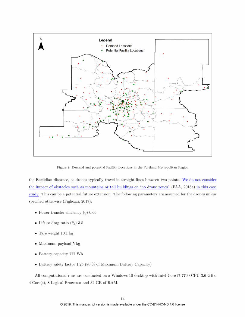
Figure 2: Demand and potential Facility Locations in the Portland Metropolitan Region

the Euclidian distance, as drones typically travel in straight lines between two points. We do not consider

the impact of obstacles such as mountains or tall buildings or “no drone zones” (FAA, 2018a) in this case

study. This can be a potential future extension. The following parameters are assumed for the drones unless

specified otherwise (Figliozzi, 2017):

• Power transfer efficiency (η) 0.66

• Lift to drag ratio (θs) 3.5

• Tare weight 10.1 kg

• Maximum payload 5 kg

• Battery capacity 777 Wh

• Battery safety factor 1.25 (80 % of Maximum Battery Capacity)

All computational runs are conducted on a Windows 10 desktop with Intel Core i7-7700 CPU 3.6 GHz,

4 Core(s), 8 Logical Processor and 32 GB of RAM.

14


5.1. Computational Efficiency

Computational efficiency of MCFLPD solutions is a key factor in real-world implementations. Initial

conditions associated to customer demands and/or weather conditions (wind direction and speed) may

change suddenly and may require a fast global reoptimization of the MCFLPD with different safety factors

(a change in regional weather conditions will affect the energy consumption of all deliveries). A later section

describes a sensitivity analysis based on different levels of allowable battery consumption. The Portland

Case Study is solved using the following three methods:

• Gurobi solver using the Python interface. The model is run for a maximum of 7200 seconds or until a

solution is obtained. Default parameters are assumed for the Gurobi Solver.

• Greedy Heuristic which is implemented in Python.

• Three Stage Heuristic (3SH): The facility location allocation problem in stage 1 and knapsack problems

in stage 2 are solved using Gurobi. The number of facilities to be exchanged in the third stage is fixed

at 2 unless specified otherwise. The exchange heuristic is run for a maximum of 100 iterations.

The first set of computational runs aim at comparing the computational efficiency of the greedy heuristic

and 3SH with the Gurobi solver for different maximum number of facilities and drone availabilities (see Table

1). Since the facilities to be exchanged are picked randomly in 3SH, we run 30 instances and report the

average, minimum, and maximum computational times as well as coverage results. We limit the number of

facilities to be exchanged in the third stage of 3SH to just two. Coverage for the purpose of this paper is

defined as the percentage of total demand met.

15


p |K|Gurobi Greedy 3SH

Time(sec)

Coverage(%)

Gap(%)

Coverage at1800 sec (%)

Time(sec)

Coverage(%)

Time (sec) Coverage (%)S2 Ave Min Max S2 Ave Min Max

5 20 7200 56.4 2.1 56.3 0.1 45.2 1.1 14.7 14.4 15.0 52.7 54.5 53.6 55.15 25 7200 61.9 2.0 61.7 0.1 50.3 1.1 15.9 15.6 16.2 58.3 59.5 58.6 60.25 30 7200 66.3 1.9 66.2 0.1 55.3 1.1 16.7 16.4 17.1 62.9 63.7 62.9 64.55 35 7200 70.2 1.2 69.5 0.1 58.9 1.2 18.3 17.6 22.8 66.5 67.0 66.5 67.95 40 7200 72.7 1.6 72.6 0.1 62.5 1.2 18.8 18.2 19.1 69.0 69.9 69.1 70.510 20 7200 64.4 2.5 64.4 0.2 48.2 1.1 16.6 16.1 16.9 59.1 61.4 59.8 62.610 30 7200 75 3.1 75 0.2 59.8 1.1 18.3 17.9 19.0 67.9 71.5 70.1 72.910 40 7200 83.8 1.7 83.8 0.2 67.1 1.1 20.1 19.2 20.8 70.2 78.4 76.3 80.415 30 7200 79.7 3.8 79.2 0.2 59.2 1.0 21.9 21.4 22.7 70.3 75.2 73.2 77.215 45 7200 90.2 1.7 89.8 0.2 73.1 1.0 24.3 23.4 25.5 74.4 83.9 80.3 86.615 60 7200 92.6 1.3 92.5 0.3 73.1 1.0 24.8 23.6 25.7 74.4 85.0 81.2 88.720 20 7200 71.2 2.1 71.1 0.3 52.8 1.0 25.1 24.6 25.6 61.7 65.8 63.2 67.520 40 7200 90.4 2.4 89.9 0.3 70.7 1.0 28.7 28.1 29.3 77.5 84.2 82.7 85.320 60 320 93.8 0.0 NA 0.3 72.2 1.0 30.4 28.6 31.8 78.9 87.2 83.6 90.120 80 36 93.8 0.0 NA 0.4 72.2 1.0 30.9 29.6 32.8 78.9 87.5 83.6 91.325 25 7200 79.6 3.5 79.5 0.3 53.6 1.0 33.0 32.1 35.0 67.3 71.5 69.2 73.325 50 337 93.8 0.0 NA 0.4 71.4 1.0 36.6 35.7 38.3 80.1 88.9 85.2 92.225 75 27 93.8 0.0 NA 0.5 71.4 1.0 37.4 36.2 39.0 80.1 88.2 84.2 91.025 100 43 93.8 0.0 NA 0.5 71.4 1.0 38.1 36.9 39.5 80.1 89.5 86.1 92.230 30 7200 85.3 4.1 84.2 0.3 60.6 1.0 40.3 39.0 41.7 72.9 76.8 74.4 80.230 60 23 93.8 0.0 NA 0.5 74.8 1.0 44.3 43.3 45.5 86.2 90.9 88.7 92.830 90 31 93.8 0.0 NA 0.6 74.7 1.0 45.1 44.2 46.4 86.2 90.7 88.7 93.0NA = Not ApplicableS2 = After Step 2

Table 1: Comparision of Gurobi solver, Greedy Heuristic, and 3SH

16


The greedy heuristic achieves 78.01% value of Gurobi on average (Best: 85.9% of Gurobi solution for

p = 5, |K| = 40; Worst: 67.36% of Gurobi solution p = 25, |K| = 25). The greedy heuristic provides

solutions which are on average within 20% of the best Gurobi solution but takes a maximum computational

time of only 0.6 seconds. According to the approximation algorithms literature in facility location, greedy

and approximate algorithm solutions differ from optimal solutions in the worst case by at least 33 % (Shmoys

et al., 1997; Jain and Vazirani, 2001). The MCFLPD is a more complex variant of facility location problems.

Therefore, we expect the worst case bounds to be weaker. However, we note empirically that all solutions

are well within the worst case bounds for facility location problems. Gurobi solver successfully finds optimal

solutions as resources become abundant (p increases and maximum available drones increases). Gurobi finds

the true optimal solution, within the 2-hour runtime limit, in nearly one-third of the cases all of which have

higher than 20 potential facility locations and at least 50 drones.

The average 3SH solutions are nearly 95% of the best Gurobi solutions on average. The best case is

when 3SH achieves 96.9% of Gurobi solution for p = 5, |K| = 20 and p = 30, |K| = 60. In the worst

case, 3SH achieves 90% of Gurobi solution for 25 potential facility locations and 25 maximum number of

drones. The 3SH approach is significantly faster than Gurobi; the median reduction in computational time is

99.7%. When the r-exchange heuristic is not run, i.e., the heuristic is stopped after repeated applications of

the knapsack problem, the heuristic provides solutions which are on an average within 85.9% of the Gurobi

solution with an average computational time of 1.2 seconds. The local search step takes an additional 26

seconds on average but helps improve the solution by another 9% making it close to the optimal solution.

Table 2 presents the average energy consumed per percent coverage which is calculated as follows:

Energy/Coverage =Average Battery Used×Number of Drones Used

Coverage

Table 2 shows that Gurobi is competitive against 3SH when the number of facilities is less, but starts

losing edge when p becomes 15 or greater and progressively worsens against 3SH with an increase in p. The

effect is also amplified with an increase in |K|, for the same p. This shows that 3SH is much more efficient

in terms of drone employment to achieve a similar coverage.

5.2. Coverage Analysis

In this section, we analyze one scenario with low coverage and one scenario with high coverage: (i) p =

5 and |K| = 35 with an optimal coverage of 70.2%, and (ii) p = 20 and |K| = 60 with an optimal coverage

of 93.8%. Figure 3 shows the delivery mapping of Gurobi solution for case (i). The delivery spiders are

distinct and do not overlap over one another. The minimum facility utilization is 23.9% of its total capacity,

and the maximum facility utilization is 87.8% of its total capacity. These results indicate that drone battery

range capacity is constraining the coverage. With five facilities, most of the demand locations around the

downtown region are covered which is intuitive as this is the area with the highest density. Coverage is

limited in low-density areas, e.g., the Northeast region.

17


Figure 3: Case (i): Gurobi Solution (p = 5 and |K| = 35)

18


p |K| Gurobi Greedy 3SH5 20 213.9 205.7 213.35 25 234.1 224.7 235.15 30 259.3 242.7 257.35 35 293.4 266.1 285.45 40 310.5 291.9 308.210 20 183.7 180.9 178.110 30 226.3 217.3 227.110 40 274.4 268.1 268.415 30 213.7 219.3 208.815 45 275.8 277.6 258.115 60 347.5 277.6 268.720 20 158.4 144.0 149.220 40 241.7 233.6 225.720 60 329.7 250.1 253.320 80 386.3 250.1 253.825 25 169.7 165.5 152.925 50 274.4 249.1 239.725 75 372.2 249.1 240.725 100 416.3 249.1 242.630 30 180.0 174.4 161.130 60 309.5 248.2 227.530 90 394.2 248.3 230.7

Table 2: Battery energy consumed per unit of coverage

Unmet Demand ZCTA Closest Facility ID Battery Requirement (Wh)97028 56 111897049 56 85497064 23 77997144 66 75098610 10 69198616 2 1624

Table 3: Summary of Unmet Demand Points for case (ii)

Figure 4 shows the delivery maps of Gurobi solution with 20 open facility and 60 available UAVs for case

(ii). It can also be seen from the figure that the central region has a lot of overlapping spiders, which suggests

that facilities have reached their capacity. The maximum facility utilization is 100% and the minimum facility

utilization is 39.1% of their total capacity. Figure 5 visualizes the facilities which have utilized more than

85% of their capacity. Most of the facilities with more than 85% capacity utilization are in the downtown

region. The demand points which are not served in this case are beyond the range of the drone from any

community center and therefore will require improvements in battery capacity (see Table 3). The battery

capacity improvements needed to achieve 100% coverage is studied in Section 5.5. The insights obtained are

consistent with (Choi and Schonfeld, 2017) on the increased effectiveness of drone delivery systems in higher

demand density regions and Dorling et al. (2017) on the critical nature of batteries.

We also compare the solutions obtained from 3SH and Greedy algorithm with the Gurobi solution. From

Figures 5, 6, and 7, it can be observed that facilities are more spatially dispersed in the Gurobi solution. The

19


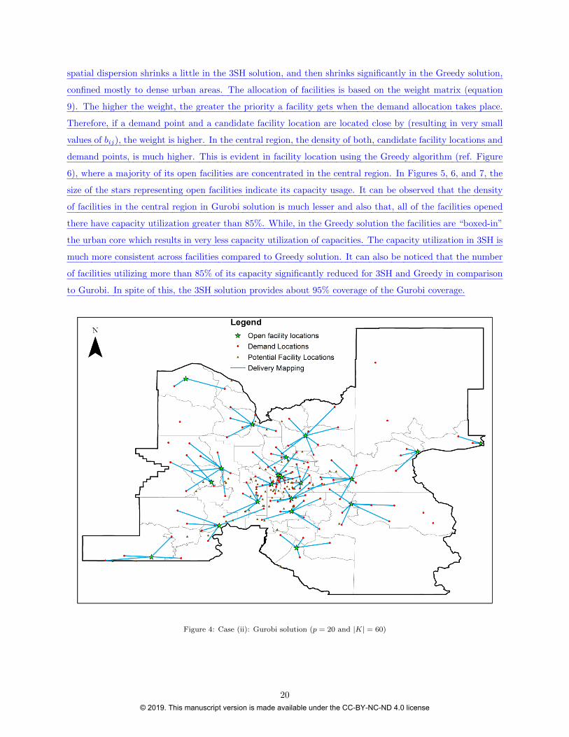
spatial dispersion shrinks a little in the 3SH solution, and then shrinks significantly in the Greedy solution,

confined mostly to dense urban areas. The allocation of facilities is based on the weight matrix (equation

9). The higher the weight, the greater the priority a facility gets when the demand allocation takes place.

Therefore, if a demand point and a candidate facility location are located close by (resulting in very small

values of bij), the weight is higher. In the central region, the density of both, candidate facility locations and

demand points, is much higher. This is evident in facility location using the Greedy algorithm (ref. Figure

6), where a majority of its open facilities are concentrated in the central region. In Figures 5, 6, and 7, the

size of the stars representing open facilities indicate its capacity usage. It can be observed that the density

of facilities in the central region in Gurobi solution is much lesser and also that, all of the facilities opened

there have capacity utilization greater than 85%. While, in the Greedy solution the facilities are “boxed-in”

the urban core which results in very less capacity utilization of capacities. The capacity utilization in 3SH is

much more consistent across facilities compared to Greedy solution. It can also be noticed that the number

of facilities utilizing more than 85% of its capacity significantly reduced for 3SH and Greedy in comparison

to Gurobi. In spite of this, the 3SH solution provides about 95% coverage of the Gurobi coverage.

Figure 4: Case (ii): Gurobi solution (p = 20 and |K| = 60)

20


Figure 5: Case (ii): Gurobi solution highlighting facilities which have greater than 85% utilization (p = 20 and |K| = 60). Sizeof star corresponds to facility utilization.

21


Figure 6: Greedy solution highlighting facilities which have greater than 85% utilization (p = 20 and |K| = 60). Size of starcorresponds to facility utilization.

22


Figure 7: 3SH solution highlighting facilities which have greater than 85% utilization (p = 20 and |K| = 60). Size of starcorresponds to facility utilization.

23


pPercent deviation with respect to 80% MBU

70% MBU 75% MBU 85% MBU 90% MBU Range5 -7.5 -3.5 2.1 4.2 11.810 -5.9 -3.9 1.7 4.3 10.315 -4.8 -2.1 1.8 3.9 8.820 -4.5 -2.0 1.8 4.0 8.525 -4.2 -1.7 1.1 3.0 7.330 -4.0 -2.3 1.4 3.1 7.2

Table 4: Variation of percent deviation in average coverage with respect to the average coverage achieved at 80% MBU

5.3. Sensitivity to Battery Safety Factor

In the initial set of experiments, the battery safety factor is set to be 1.25 (drones cannot utilize more

than 80% of the battery capacity) to account for weather-related uncertainties, battery usage during take-

off and landing, and uncertainties regarding initial battery conditions (Figliozzi, 2017; Microdrones, 2018).

The goal of this set of experiments is to study the impact of the variation in battery safety factor on the

coverage. The battery safety factor considered in this analysis include safety factors 10/7.0, 10/7.5, 10/8.5,

and 10/9.0. These correspond to 70%, 75%, 85%, and 90% of the battery capacity respectively. Table 4

presents the average of percentage deviation of coverage at specified maximum battery utilization (MBU)

from the coverage achieved assuming a maximum battery utilization of 80% across 30 runs.

Percent Deviation =

30∑i=1

Coverageix − Coveragei80Coveragei80

× 100

Coveragei80 represents the coverage at 80% maximum battery utilization and Coverageix is the coverage

at x % maximum battery utilization in the ith run of 3SH. In general, the effects of having a high battery

safety factor (less available energy) are more profound than the effects of a low battery safety factor (more

available energy). As shown in Table 4, the effect of the battery safety factor decreases marginally as p (the

number of open facilities) increases.

5.4. Sensitivity to number of facilities to be exchanged in 3SH

In all the runs completed until now, two facilities (two removed and added) were exchanged in the third

step of the 3SH heuristic. We now vary the number of facilities to be exchanged and study the variation in

computational times and improvement in coverage. The values presented in Table 5 are the average of 30

runs. A 1 facility exchange in 3SH works best when p = 5; a 2 facility exchange in 3SH works best when

p = 10, and a 3 facility exchange in 3SH works best for p ≥ 15. No benefits were found when the number of

facilities exchanged was 4 or higher. The runtimes are comparable on average which is expected given that

the underlying problem sizes are not significantly altered by the size of the exchange procedure.

5.5. Sensitivity to changes in Battery Capacity

This section shows how coverage would improve with changes in the battery capacity of the drone. All

instances were solved using Gurobi. The ideal scenario portrays the improvement in the battery without

24


p |K|After Step 2 1 facility exchange 2 facility exchange 3 facility exchange

Coverage Time Coverage Time Coverage Time Coverage Time(%) (sec) (%) (sec) (%) (sec) (%) (sec)

5 20 52.7 1.1 54.4 15.4 54.5 14.7 53.8 13.55 25 58.3 1.1 60.0 16.1 59.5 15.9 59.0 14.35 30 62.9 1.1 64.5 17.2 63.7 16.7 63.3 15.15 35 66.5 1.2 67.8 18.0 67.0 18.3 66.9 15.95 40 69.0 1.2 70.4 18.8 69.9 18.8 69.9 16.610 20 59.1 1.1 60.8 15.5 61.4 16.6 61.0 15.710 30 67.9 1.1 70.4 17.3 71.5 18.3 71.2 17.210 40 70.2 1.1 76.7 18.7 78.4 20.1 78.4 18.515 30 70.3 1.0 74.2 20.8 75.2 21.9 75.2 20.515 45 74.4 1.1 82.2 22.7 83.9 24.3 84.8 22.415 60 74.4 1.1 82.4 22.9 85.0 24.8 86.2 22.720 20 61.7 1.1 65.7 24.2 65.8 25.1 66.3 23.420 40 77.5 1.1 83.6 27.4 84.2 28.7 84.5 26.220 60 78.9 1.1 85.0 28.8 87.2 30.4 88.6 27.320 80 78.9 1.1 84.9 29.1 87.5 30.9 88.9 27.425 25 67.3 1.1 71.1 31.3 71.5 33.0 72.0 29.425 50 80.1 1.1 87.8 35.3 88.9 36.6 90.2 32.225 75 80.1 1.1 87.0 35.8 88.2 37.4 89.4 32.325 100 80.1 1.1 86.6 36.4 89.5 38.1 90.2 32.330 30 72.9 1.1 76.9 38.4 76.8 40.3 77.1 34.230 60 86.2 1.1 89.5 42.8 90.9 44.3 91.5 37.030 90 86.2 1.1 89.3 43.4 90.7 45.1 91.1 37.0

Table 5: Impact of different number of facilities exchanged in 3SH

an increase in the drone tare weight, which may be possible due to future breakthroughs in the battery

technology. The realistic scenario assumes that we can improve the battery capacity of a drone by adding

additional batteries. This results in an increase in drone tare weight which leads to increased battery

consumption for the same amount of distance traveled. The UAV/drone in consideration uses Lithium

polymer (LiPo) batteries. It is reported that the specific energy of LiPo batteries can go up to 275 Wh/kg

(Amicell, 2018). So, for the realistic case study, the specific energy is taken to be 255 Wh/kg with 80% MBU.

The analysis is conducted for the case when p = 20, |K| = 60. It is observed that about 165% increase in the

battery capacity is required to achieve full coverage in the ideal case (see Table 6). In the realistic scenario,

this increase is still not sufficient to achieve 100% coverage. This is because, the increase in distance traveled

is not as high as in the ideal case due to the additional battery consumption.

An important conclusion from the sensitivity analysis is that runtime increases substantially as battery

capacity increases. This is likely the result of additional complexity due to the increase of feasible options

that must be analyzed by the MIP solver. Hence, the value of a high quality and yet computationally efficient

heuristic like 3SH is likely to increase substantially in the future.

25


BatteryIdeal Realistic

Tare Mass Coverage(%) Time (sec) Tare Mass Coverage(%) Time (sec)777 10.1 93.8 410 10.1 93.8 4101032 10.1 96.7 1233 11.1 95.7 6671287 10.1 97.4 1204 12.1 97.4 9781542 10.1 98.7 2212 13.1 97.4 8731797 10.1 98.7 2557 14.1 97.4 14752052 10.1 100 2070 15.1 98.7 1377

Table 6: Impact of Battery Capacity on Coverage

6. Conclusions

This paper presents a novel model denoted MCFLPD for coverage-based capacitated facility location

problem with drones by factoring in real-life UAV battery and weight constraints. MCFLPD is substantially

more complex than traditional capacitated facility location problems. As real-world drone-based deliveries

have already started being implemented in the field, it is necessary to study facility location for drones

not only for economic purposes but also for social/humanitarian benefit. Drone deliveries tend to be time-

sensitive, e.g. medical supplies, and/or subject to unexpected changes in weather conditions. Hence, solution

times are as important as solution quality.

In this research, three solution approaches are presented and compared. A state of the art MIP solver

deliver high-quality solutions but requires unacceptably long running times to find feasible solutions reliably.

A greedy algorithm is extremely fast, less than one second on average, but at the cost of solution quality

(nearly 20% coverage loss). The three-stage heuristics (3SH) is based on decomposition and local exchange

principles and on average the 3SH solutions are within 5% of the best Gurobi solutions but require in all cases

substantially less running time (at most 46 seconds). The 3SH heuristic achieves this balanced performance

by leveraging the problem structure to obtain solutions with high coverage but also more economical in terms

of drone employment and in an appropriate time.

The sensitivity analysis on the battery safety factors suggests that the effects of increasing battery safety

are acute. An analysis to estimate the technological improvement in the battery capacity was also performed.

It showed that a breakthrough in battery technology is required to achieve one hundred percent coverage for

the case study considered in this work. It was also demonstrated that MIP solver (Gurobi) solution times

increase substantially as battery technology increases. This result further enhances the value of an efficient

algorithm such as the proposed 3SH heuristic.

7. References

Agatz, N., Bouman, P., Schmidt, M., 2018. Optimization approaches for the traveling salesman problem

with drone. Transportation Science.

Albareda-Sambola, M., Fernandez, E., Laporte, G., 2009. The capacity and distance constrained plant

location problem. Computers & Operations Research 36 (2), 597–611.

26


Albornoz, C., Giraldo, L. F., 2017. Trajectory design for efficient crop irrigation with a uav. In: 2017 IEEE

3rd Colombian Conference on Automatic Control (CCAC). IEEE, pp. 1–6.

Amazon, 2018. Amazon prime air. Accessed: May 2018.

URL https://www.amazon.com/Amazon-Prime-Air/b?ie=UTF8&node=8037720011

Amicell, 2018. Li-polymer batteries. Accessed: May 2018.

URL http://www.amicell.co.il/batteries/rechargeable-batteries/li-polymer-batteries/

Amukele, T., Ness, P. M., Tobian, A. A., Boyd, J., Street, J., 2017. Drone transportation of blood products.

Transfusion 57 (3), 582–588.

Anaya-Arenas, A. M., Renaud, J., Ruiz, A., 2014. Relief distribution networks: a systematic review. Annals

of Operations Research 223 (1), 53–79.

Berner, B., Chojnacki, J., 2017. Use of drones in crop protection. In: IX International Scientific Symposium

“Farm Machinery and Processes Management in Sustainable Agriculture”. IEEE, pp. 46–51.

Boutilier, J. J., Brooks, S. C., Janmohamed, A., Byers, A., Buick, J. E., Zhan, C., Schoellig, A. P., Cheskes,

S., Morrison, L. J., Chan, T. C., 2017. Optimizing a drone network to deliver automated external defib-

rillators. Circulation, 2454–2465.

Burema, H., Filin, A., 2016. Aerial farm robot system for crop dusting, planting, fertilizing and other field

jobs. US Patent 9,382,003.

Carlsson, J. G., Song, S., 2017. Coordinated logistics with a truck and a drone. Management Science.

Choi, Y., Schonfeld, P. M., 2017. Optimization of multi-package drone deliveries considering battery capacity.

In: 96th Annual Meeting of the Transportation Research Board, Washington, DC (Paper No. 17–05769).

Chowdhury, S., Emelogu, A., Marufuzzaman, M., Nurre, S. G., Bian, L., 2017. Drones for disaster response

and relief operations: a continuous approximation model. International Journal of Production Economics

188, 167–184.

Church, R., ReVelle, C., 1974. The maximal covering location problem. In: Papers of the Regional Science

Association. Vol. 32(1). Springer, pp. 101–118.

Claesson, A., Backman, A., Ringh, M., Svensson, L., Nordberg, P., Djarv, T., Hollenberg, J., 2017. Time to

delivery of an automated external defibrillator using a drone for simulated out-of-hospital cardiac arrests

vs emergency medical services. Jama 317 (22), 2332–2334.

Costa, F. G., Ueyama, J., Braun, T., Pessin, G., Osorio, F. S., Vargas, P. A., 2012. The use of unmanned

aerial vehicles and wireless sensor network in agricultural applications. In: Geoscience and Remote Sensing

Symposium (IGARSS), 2012 IEEE International. IEEE, pp. 5045–5048.

27


Daknama, R., Kraus, E., 2017. Vehicle routing with drones. eprint arXiv:1705.06431.

URL https://arxiv.org/pdf/1705.06431.pdf

Daskin, M. S., 2011. Network and discrete location: models, algorithms, and applications. John Wiley &

Sons.

Dayarian, I., Savelsbergh, M., Clarke, J.-P., 2017. Same-day delivery with drone resupply. Optimization

online.

URL http://www.optimization-online.org/DB_FILE/2017/09/6206.pdf

DHL, 2014. Unmanned aerial vehicles in logistics: A dhl perspective on implications and use for the logistics

industry. Accessed: May 2018.

URL http://www.dhl.com/content/dam/downloads/g0/about_us/logistics_insights/DHL_

TrendReport_UAV.pdf

Dorling, K., Heinrichs, J., Messier, G. G., Magierowski, S., 2017. Vehicle routing problems for drone delivery.

IEEE Transactions on Systems, Man, and Cybernetics: Systems 47 (1), 70–85.

FAA, 2018a. Airspace restrictions. Accessed: Dec 2018.

URL https://www.faa.gov/uas/where_to_fly/airspace_restrictions/

FAA, 2018b. Faa begins drone airspace authorization expansion. Accessed: May 2018.

URL https://www.faa.gov/news/updates/?newsId=90245

Faical, B. S., Costa, F. G., Pessin, G., Ueyama, J., Freitas, H., Colombo, A., Fini, P. H., Villas, L., Osorio,

F. S., Vargas, P. A., et al., 2014. The use of unmanned aerial vehicles and wireless sensor networks for

spraying pesticides. Journal of Systems Architecture 60 (4), 393–404.

Farahani, R. Z., Asgari, N., Heidari, N., Hosseininia, M., Goh, M., 2012. Covering problems in facility

location: A review. Computers & Industrial Engineering 62 (1), 368–407.

Fehrenbacher, K., 2018. A new lithium-metal battery takes flight in drones. Accessed: May 2018.

URL https://www.greentechmedia.com/articles/read/a-new-lithium-metal-battery-takes-flight-in-drones#

gs.s_bKMvI

Figliozzi, M., 2017. Lifecycle modeling and assessment of unmanned aerial vehicles (Drones) CO2e emissions.

Transportation Research Part D 57, 251–261.

Giles, D. K., Billing, R., Singh, W., 2016. Performance results, economic viability and outlook for remotely

piloted aircraft for agricultural spraying. Aspects of Applied Biology 132, 15–21.

Golabi, M., Shavarani, S. M., Izbirak, G., 2017. An edge-based stochastic facility location problem in uav-

supported humanitarian relief logistics: a case study of tehran earthquake. Natural Hazards 87 (3), 1545–

1565.

28


Goodchild, A., Toy, J., 2017. Delivery by drone: An evaluation of unmanned aerial vehicle technology in

reducing co2 emissions in the delivery service industry. Transportation Research Part D: Transport and

Environment.

Goundan, P. R., Schulz, A. S., 2007. Revisiting the greedy approach to submodular set function maximiza-

tion. Optimization online.

URL http://www.optimization-online.org/DB_FILE/2007/08/1740.pdf

Ha, Q. M., Deville, Y., Pham, Q. D., Ha, M. H., 2018. On the min-cost traveling salesman problem with

drone. Transportation Research Part C: Emerging Technologies 86, 597–621.

Halper, R., Raghavan, S., Sahin, M., 2015. Local search heuristics for the mobile facility location problem.

Computers & Operations Research 62, 210–223.

Hassanalian, M., Abdelkefi, A., 2017. Classifications, applications, and design challenges of drones: A review.

Progress in Aerospace Sciences 99, 99–131.

Holguın-Veras, J., Jaller, M., Van Wassenhove, L. N., Perez, N., Wachtendorf, T., 2012. On the unique

features of post-disaster humanitarian logistics. Journal of Operations Management 30 (7-8), 494–506.

Hong, I., Kuby, M., Murray, A. T., 2018. A range-restricted recharging station coverage model for drone

delivery service planning. Transportation Research Part C: Emerging Technologies 90, 198–212.

Jain, K., Vazirani, V. V., 2001. Approximation algorithms for metric facility location and k-median problems

using the primal-dual schema and lagrangian relaxation. Journal of the ACM (JACM) 48 (2), 274–296.

Kang, J., Park, S., 2003. Algorithms for the variable sized bin packing problem. European Journal of Oper-

ational Research 147(2), 365–372.

Karaca, Y., Cicek, M., Tatli, O., Sahin, A., Pasli, S., Beser, M. F., Turedi, S., 2018. The potential use

of unmanned aircraft systems (drones) in mountain search and rescue operations. American Journal of

Emergency Medicine 36, 585–588.

Kim, S. J., Lim, G. J., Cho, J., 2018. Drone flight scheduling under uncertainty on battery duration and air

temperature. Computers & Industrial Engineering 117, 291–302.

Kim, S. J., Lim, G. J., Cho, J., Cote, M. J., 2017. Drone-aided healthcare services for patients with chronic

diseases in rural areas. Journal of Intelligent & Robotic Systems 88 (1), 163–180.

Li, K.-R., See, K.-Y., Koh, W.-J., Zhang, J.-W., 2017. Design of 2.45 ghz microwave wireless power trans-

fer system for battery charging applications. In: Progress in Electromagnetics Research Symposium-Fall

(PIERS-FALL). IEEE, pp. 2417–2423.

29


Loulou, R., Michaelides, E., 1979. New greedy-like heuristics for the multidimensional 0-1 knapsack problem.

Operations Research 27(6), 1101–1114.

Mack, E., 2018. How delivery drones can help save the world. Accessed: May 2018.

URL https://www.forbes.com/sites/ericmack/2018/02/13/delivery-drones-amazon-energy-efficient-reduce-climate-change-pollution/

#476a63f56a87

Melo, M. T., Nickel, S., Saldanha-Da-Gama, F., 2009. Facility location and supply chain management–a

review. European journal of operational research 196(2), 401–412.

Microdrones, 2018. The heavy lifting drone - md4300. Accessed: May 2018.

URL https://www.amazon.com/Amazon-Prime-Air/b?ie=UTF8&node=8037720011

Murray, C. C., Chu, A. G., 2015. The flying sidekick traveling salesman problem: Optimization of drone-

assisted parcel delivery. Transportation Research Part C: Emerging Technologies 54, 86–109.

Otto, A., Agatz, N., Campbell, J., Golden, B., Pesch, E., 2018. Optimization approaches for civil applications

of unmanned aerial vehicles (uavs) or aerial drones: A survey. Networks.

URL https://doi.org/10.1002/net.21818

Ozdamar, L., 2011. Planning helicopter logistics in disaster relief. OR spectrum 33 (3), 655–672.

Pirkul, H., Schilling, D., 1989. The capacitated maximal covering location problem with backup service.

Annals of Operations Research 18 (1), 141–154.

Poikonen, S., Wang, X., Golden, B., 2017. The vehicle routing problem with drones: Extended models and

connections. Networks 70 (1), 34–43.

Ponza, A., 2016. Optimization of drone-assisted parcel delivery. Master’s thesis, University of Padova.

Puchinger, J., Raidl, G. R., 2007. Models and algorithms for three-stage two-dimensional bin packing.

European Journal of Operational Research 183 (3), 1304–1327.

Pulver, A., Wei, R., 2018. Optimizing the spatial location of medical drones. Applied Geography 90, 9–16.

Scott, J. E., Scott, C. H., 2018. Models for drone delivery of medications and other healthcare items.

International Journal of Healthcare Information Systems and Informatics (IJHISI) 13 (3), 20–34.

Shmoys, D. B., Tardos, E., Aardal, K., 1997. Approximation algorithms for facility location problems. In:

Proceedings of the twenty-ninth annual ACM symposium on Theory of computing. ACM, pp. 265–274.

Thiels, C., Aho, J., Zietlow, S., Jenkins, D., 2015. Use of unmanned aerial vehicles for medical product

transport. Air Medical Journal 34 (2), 104–108.

30


Wang, C., He, X., Liu, Y., Song, J., Zeng, A., 2016. The small single and multirotor unmanned aircraft

vehicles chemical application techniques and control for rice fields in china. Aspects of Applied Biology

132, 73–81.

Wang, X., Poikonen, S., Golden, B., 2017. The vehicle routing problem with drones: Several worst-case

results. Optimization Letters 11 (4), 679–697.

Wu, T.-H., Low, C., Bai, J.-W., 2002. Heuristic solutions to multi-depot location-routing problems. Com-

puters & Operations Research 29(10), 1393–1415.

Yanmaz, E., Quaritsch, M., Yahyanejad, S., Rinner, B., Hellwagner, H., Bettstetter, C., 2017. Communica-

tion and coordination for drone networks. In: Ad Hoc Networks. Springer, pp. 79–91.

Yanmaz, E., Yahyanejad, S., Rinner, B., Hellwagner, H., Bettstetter, C., 2018. Drone networks: Communi-

cations, coordination, and sensing. Ad Hoc Networks 68, 1–15.

Yurek, E. E., Ozmutlu, H. C., 2018. A decomposition-based iterative optimization algorithm for traveling

salesman problem with drone. Transportation Research Part C: Emerging Technologies 91, 249–262.

31


Appendix A. List of Demand Points and Candidate Facility Locations

32


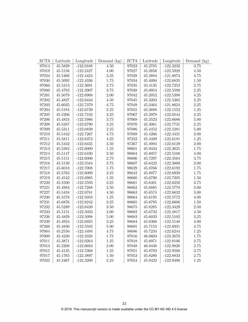
ZCTA Latitude Longitude Demand (kg) ZCTA Latitude Longitude Demand (kg)97014 45.5829 -122.0168 4.50 97023 45.2785 -122.3232 3.7597019 45.5156 -122.2427 4.00 97027 45.3856 -122.5928 4.5097024 45.5466 -122.4424 3.25 97028 45.2884 -121.8074 4.7597030 45.5092 -122.4336 1.75 97034 45.4094 -122.6835 1.5097060 45.5313 -122.3691 2.75 97035 45.4135 -122.7252 2.7597080 45.4783 -122.3907 3.75 97038 45.0954 -122.5590 2.2597201 45.5079 -122.6908 2.00 97042 45.2052 -122.5398 4.2597202 45.4827 -122.6444 4.50 97045 45.3203 -122.5365 2.2597203 45.6035 -122.7379 4.75 97049 45.3464 -121.8624 2.2597204 45.5184 -122.6739 2.25 97055 45.3888 -122.1552 1.2597205 45.5206 -122.7102 3.25 97067 45.2978 -122.0544 3.2597206 45.4824 -122.5986 3.75 97068 45.3523 -122.6686 5.0097208 45.5287 -122.6790 3.25 97070 45.3061 -122.7731 2.2597209 45.5311 -122.6839 2.25 97086 45.4452 -122.5281 5.0097210 45.5442 -122.7267 4.75 97089 45.4266 -122.4431 3.0097211 45.5811 -122.6373 4.25 97222 45.4409 -122.6181 1.2597212 45.5442 -122.6435 3.50 97267 45.4084 -122.6129 2.0097213 45.5382 -122.6000 1.25 98601 45.9434 -122.3625 1.7597214 45.5147 -122.6430 2.50 98604 45.8057 -122.5108 4.0097215 45.5151 -122.6006 2.75 98606 45.7297 -122.4564 3.7597216 45.5139 -122.5584 2.75 98607 45.6422 -122.3800 3.0097217 45.6018 -122.7008 1.75 98629 45.8766 -122.6192 1.7597218 45.5763 -122.6009 3.25 98642 45.8077 -122.6939 1.7597219 45.4542 -122.6985 1.25 98660 45.6790 -122.7205 1.5097220 45.5500 -122.5593 3.25 98661 45.6401 -122.6250 3.7597221 45.4983 -122.7288 2.50 98662 45.6885 -122.5778 3.0097227 45.5434 -122.6781 4.50 98663 45.6574 -122.6632 3.0097230 45.5578 -122.5053 1.25 98664 45.6195 -122.5772 4.0097231 45.6876 -122.8242 3.25 98665 45.6795 -122.6606 1.5097232 45.5289 -122.6439 3.50 98675 45.8285 -122.3429 2.5097233 45.5151 -122.5033 2.00 98682 45.6732 -122.4817 4.5097236 45.4829 -122.5098 5.00 98683 45.6033 -122.5102 3.2597239 45.4924 -122.6925 3.25 98684 45.6306 -122.5148 4.0097266 45.4830 -122.5582 5.00 98685 45.7152 -122.6931 4.7597004 45.2550 -122.4494 4.75 98686 45.7234 -122.6244 1.2597009 45.4230 -122.3328 1.75 97016 46.0603 -123.2670 1.7597011 45.3871 -122.0264 1.25 97018 45.8971 -122.8106 2.7597013 45.2208 -122.6683 2.00 97048 46.0448 -122.9820 2.7597015 45.4135 -122.5368 1.25 97051 45.8793 -122.9500 3.7597017 45.1765 -122.3897 1.50 97053 45.8280 -122.8833 2.7597022 45.3467 -122.3200 2.25 97054 45.9422 -122.9496 1.25

33


ZCTA Latitude Longitude Demand (kg) ZCTA Latitude Longitude Demand (kg)97056 45.7720 -122.9694 4.50 97116 45.5808 -123.1657 2.0097064 45.8591 -123.2355 4.00 97117 45.6314 -123.2884 3.0097101 45.0902 -123.2287 4.25 97119 45.4689 -123.2002 3.2597111 45.2845 -123.1952 3.75 97123 45.4402 -122.9801 2.7597114 45.1879 -123.0766 3.75 97124 45.5698 -122.9496 2.2597115 45.2752 -123.0395 3.50 97125 45.6711 -123.1969 1.7597127 45.2461 -123.1114 4.25 97133 45.6861 -123.0227 3.5097128 45.2119 -123.2822 4.25 97140 45.3531 -122.8659 4.5097132 45.3242 -122.9873 5.00 97144 45.7416 -123.3002 2.2597148 45.3584 -123.2485 3.75 97223 45.4403 -122.7766 3.7597347 45.0771 -123.6564 1.50 97224 45.4055 -122.7951 1.7597396 45.1040 -123.5490 3.75 97225 45.5016 -122.7700 2.0097005 45.4910 -122.8036 3.25 97229 45.5510 -122.8093 2.0097006 45.5170 -122.8598 3.25 98605 45.7769 -121.6655 4.2597007 45.4543 -122.8796 2.00 98610 45.8659 -122.0652 4.7597008 45.4602 -122.8042 2.25 98616 46.1933 -122.1329 4.7597062 45.3693 -122.7623 1.75 98639 45.6699 -121.9897 1.7597106 45.6657 -123.1190 3.75 98648 45.7063 -121.9563 2.7597109 45.7378 -123.1812 3.00 98651 45.7399 -121.5835 3.5097113 45.4972 -123.0443 1.50 98671 45.6144 -122.2384 1.50

Table A.7: List of demand points with assumed demand

34


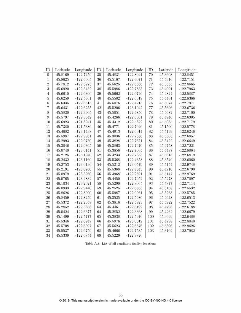
ID Latitude Longitude ID Latitude Longitude ID Latitude Longitude0 45.8169 -122.7459 35 45.4831 -122.8041 70 45.3608 -122.84511 45.8625 -122.6605 36 45.5167 -122.6071 71 45.4316 -122.71512 45.7812 -122.5273 37 45.5625 -122.6666 72 45.3535 -122.86653 45.6920 -122.5452 38 45.5986 -122.7853 73 45.4091 -122.79634 45.6610 -122.6360 39 45.5662 -122.6746 74 45.4824 -122.58875 45.6259 -122.5361 40 45.5502 -122.6619 75 45.4401 -122.83666 45.6335 -122.6613 41 45.5076 -122.4215 76 45.5074 -122.79717 45.6431 -122.6255 42 45.5206 -123.1042 77 45.5696 -122.67368 45.5820 -122.3905 43 45.5051 -122.4856 78 45.4682 -122.71009 45.5797 -122.3542 44 45.4266 -122.6061 79 45.4946 -122.630510 45.6923 -121.8941 45 45.4312 -122.5822 80 45.5085 -122.717911 45.7380 -121.5386 46 45.4771 -122.7040 81 45.1500 -122.577812 45.4682 -123.1438 47 45.4913 -122.6014 82 45.5199 -122.624613 45.5987 -122.9961 48 45.3036 -122.7586 83 45.5503 -122.685714 45.2993 -122.9750 49 45.3828 -122.7321 84 45.5422 -122.664915 45.3046 -122.9365 50 45.3863 -122.7670 85 45.4758 -122.722116 45.0740 -123.6141 51 45.3856 -122.7605 86 45.4487 -122.806417 45.2125 -123.1940 52 45.4233 -122.7685 87 45.5618 -122.681918 45.2432 -123.1160 53 45.5368 -122.4358 88 45.3549 -122.606019 45.2753 -123.0136 54 45.5212 -123.0579 89 45.5154 -122.974820 45.2191 -123.0760 55 45.5368 -122.8343 90 45.4710 -122.679021 45.0979 -123.3960 56 45.3968 -122.2691 91 45.5147 -122.976922 45.0765 -123.4832 57 45.4450 -122.7952 92 45.5278 -122.709723 46.1034 -123.2021 58 45.5290 -122.8065 93 45.5877 -122.711424 46.0933 -122.9440 59 45.2525 -122.6865 94 45.5158 -122.553225 45.8626 -122.8090 60 45.5987 -122.9961 95 45.5268 -122.578526 45.8459 -122.8259 61 45.3525 -122.5980 96 45.4648 -122.651327 45.5372 -122.2658 62 45.3816 -122.5923 97 45.5922 -122.752228 45.2852 -122.3368 63 45.4461 -122.6192 98 45.4798 -122.618829 45.0424 -122.6677 64 45.2852 -122.3368 99 45.4262 -122.667930 45.1499 -122.5777 65 45.3838 -122.5976 100 45.3699 -122.648831 45.5346 -122.6247 66 45.5976 -123.0012 101 45.4798 -122.804032 45.5708 -122.6097 67 45.5623 -122.6676 102 45.5396 -122.962633 45.5537 -122.6759 68 45.4666 -122.7535 103 45.3102 -122.798234 45.5339 -122.6854 69 45.5229 -122.9820

Table A.8: List of all candidate facility locations

35


maximum coverage capacitated facility location problem

Documents