Akimasa Fujiwara

IDEC, Hiroshima University

2004/04/22

Akimasa FujiwaraAkimasa Fujiwara

IDEC, Hiroshima UniversityIDEC, Hiroshima University

2004/04/222004/04/22

An Evaluation of Sustainable Urban Form Based

on Discrete Choice Models

A Case Study in the Jabotabek Region, Indonesia

An Evaluation of An Evaluation of Sustainable Urban Form Based Sustainable Urban Form Based

on Discrete Choice Modelson Discrete Choice Models

A Case Study in the Jabotabek A Case Study in the Jabotabek Region, IndonesiaRegion, Indonesia

Why are required to discuss on urban forms?

Human activity is strongly affected by urban form

Close relationship between human activity and transport network

Travel is a derived demand of activities

Limitation of single transportation policies

Change of life cycle stage affects on travel patterns

Environmental Sustainability in Urban Transportation

• Less road construction

• Fewer car trips/shortened vehicle miles traveled

• …

• Less road construction

• Fewer car trips/shortened vehicle miles traveled

• …

Transportation strategies

• Transportation demand management

• Transportation control measures

• Vehicle/fuel technologies

Transportation strategies

• Transportation demand management

• Transportation control measures

• Vehicle/fuel technologies

Land use strategies

• Transit Oriented Development（TOD)

• Compact city

Land use strategies

• Transit Oriented Development（TOD)

• Compact city

Transportation and Land Use Strategies

Transportation strategies

outcomes

T ravel Demand Management

T ransportation Systems

Management

Vehicle/Fuel T echnology

T rip patterns (mode, length,

time of day etc.)

Vehicle activity (vehicle-trips,

vehicle miles of travel etc.)

Air Quality

T raffic Flow (speed,

acceleration)

Land use strategies

T ransit Oriented

Development

Compact City

Relationship between LCS and residential & travel mode choices

Younger single

FrequentlyPublic transit

Younger single

FrequentlyPublic transit

Younger couple

FrequentlyCar + transit

Younger couple

FrequentlyCar + transit

Couple withjunior children

Occasionally Car2 + transit

Couple withjunior children

Occasionally Car2 + transit

Couple withsenior children

InfrequentlyCar2 + transit

Couple withsenior children

InfrequentlyCar2 + transit

Elder couple

InfrequentlyCar + transit

Elder couple

InfrequentlyCar + transit

Elder single

OccasionallyPublic transit

Elder single

OccasionallyPublic transit

Transit Oriented Development• “The practice of developing or intensifying residential land use near rail stations” (Boarnet and

Crane 1998).• “Development within a specified geographical area around a transit station with a variety of land

uses and a multiplicity of landowners” (Salvensen 1996).• “A mixed-use community that encourages people to live near transit services and to decrease

their dependence on driving” (Still 2002).• “A compact, mixed-use community, centered around a transit station that, by design, invites

residents, workers, and shoppers to drive their cars less and ride mass transit more. The transitvillage extends roughly a quarter mile from a transit station, a distance that can be covered inabout 5 minutes by foot. The centerpiece of the transit village is the transit station itself and thecivic and public spaces that surround it. The transit station is what connects village residents to the rest of the region…The surrounding public space serves the important function of being a community gathering spot, a site for special events, and a place for celebrations—a modern-day version of the Greek agora” (Bernick and Cervero 1997, p. 5).

• Mixed-use development

• Development that is close to and well-served by transit

• Development that is conducive to transit riding

• Compactness

• Pedestrian- and cycle-friendly environs

• Public and civic spaces near stations

• Stations as community hubs

Transit Oriented Developmentdifferent elements of design

Compact City• To limit distances between home and work and to aim for a better balance between living and

working;• To make the best possible use of existing facilities and infrastructure, and to improve the position

of public transport;• To use space as efficiently as possible by building connected properties in high densities;• To maintain and create varied residential environments in and on the outskirts of the city;• To fragment rural areas as little as possible and to reduce the environmental burden from road

traffic.'

• Minimum densities• Multi functionality• Concentration of development at nodes• Transformation of urban mobility• Congruence of spatial-functional structure and public transit system• Station areas as catalysts for development.

街なか居住研究会

http://www.thr.mlit.go.jp/compact-city/index.html

Newly Developing Asian CitiesBasic Characteristics

• Development of economic activities at a world scale• Spatial division of labor• Division of function between core and periphery of the city• Shift from single core to multiple cores• Land use change in the urban center, agricultural land conversion on

the periphery• Development of large scale infrastructure• Substantial increase in space production (by horizontal, vertical

expansions and renewal of old land uses)• High growth in commuters and increasing commuting time

(Firman, 1998)

JA(karta)BO(gor)TA(ngerang)BEK(asi)metropolitan area

面積＝6418ｋｍ２

Murakami et al. 2004

Cybriwsky and Ford, 2001

11,886,579

20,159,65517,131,356

0

5,000,000

10,000,000

15,000,000

20,000,000

25,000,000

1980 1990 1995

D.K.I. Jakarta

Bogor

Bekasi

Tangerang

Jabotabek Total

人口

JA(karta)BO(gor)TA(ngerang)BEK(asi)metropolitan area

Firman, 1998

D.(Daerah) K.(Khurus) I.(Ibukota) Jakarta- 1990 -

1.5 - 2.0

2.0 - 4.0

1.0 - 1.5

Population Employment RatioDaerah Khurus Ibukota (DKI) Jakarta

adapted from Kenworthy and Laube 1999

401.9

170.6

438.6

Activity Ratio (Population+# of Jobs)/AreaDaerah Khurus Ibukota (DKI) Jakarta

adopted from Kenworthy and Laube 1999

Stated Preference Survey

• Household based survey• Based on three hypothetical city forms

– Transit oriented development– Compact city– Metropolitan suburban setting

• Household makes the decision– The place of residence

• Transit oriented development• Compact city• Metropolitan suburban setting

– Commute trip mode• Private car• Bus• Train

Sample Characteristics• 303 Surveyed households

• 4 instances of choices on residence and commute mode

– (data points 303X4=1212)

• Total number of individuals in households=1536

• Average household size=5.07 (s=1.93)

• Autumn, 2003

DKI Jakarta

Bekasi

Bogor

Tangerang

# of Households Surveyed

150

140

130

120

110

100

90

80

70

60

50

40

30

20

10

0

Tangerang Region

Tangerang Mun.

Depok Mun.

Bogor Region Count

Bogor Mun.

Bekasi Region

Bekasi Mun.

Central Jakarta

West Jakarta

South Jakarta

East Jakarta

North Jakarta

Depok Municipality

Jakarta West

Jakarta Central

Jakarta South

Jakarta East

Jakarta North

Bekasi Semi-urban

Bogor Semi-urban

Tangerang Semi-urban

Bekasi Municipality

Bogor Municipality

Tangerang Mun.

Average # of Years of Residence

30.025.020.015.010.05.00.0

sample average

Depok Municipality

Jakarta West

Jakarta Central

Jakarta South

Jakarta East

Jakarta North

Bekasi Semi-urban

Bogor Semi-urban

Tangerang Semi-urban

Bekasi Municipality

Bogor Municipality

Tangerang Mun.

Average household size by sub-districts.

5.85.65.45.25.04.84.64.44.24.0

sample average

Sample Characteristics

Own House

Rented House

Company House

Count

300250200150100500

26

273

Sample Characteristics

North Jakarta

East Jakarta

South Jakarta

West Jakarta

Central Jakarta

Bekasi Municipality

Bekasi Region

Bogor Municipality

Bogor Region

Depok Municipality

Tangerang Municipali

Tangerang Region

%

100

90

80

70

60

50

40

30

20

10

0

Dist to Market = d

d > 2km

1km< d < 2km

500mt< d < 1km

d < 500mt

North Jakarta

East Jakarta

South Jakarta

West Jakarta

Central Jakarta

Bekasi Municipality

Bekasi Region

Bogor Municipality

Bogor Region

Depok Municipality

Tangerang Municipali

Tangerang Region

%

100

90

80

70

60

50

40

30

20

10

0

Dist to Restaurants

d > 2km

1km < d < 2km

500mt < d < 1km

500mt < d

North Jakarta

East Jakarta

South Jakarta

West Jakarta

Central Jakarta

Bekasi Municipality

Bekasi Region

Bogor Municipality

Bogor Region

Depok Municipality

Tangerang Municipali

Tangerang Region

%

100

90

80

70

60

50

40

30

20

10

0

Dist to Parks

d > 2km

1km < d < 2km

500mt < d < 1km

d < 500mt

North Jakarta

East Jakarta

South Jakarta

West Jakarta

Central Jakarta

Bekasi Municipality

Bekasi Region

Bogor Municipality

Bogor Region

Depok Municipality

Tangerang Municipali

Tangerang Region

%

100

90

80

70

60

50

40

30

20

10

0

D to Department St.

d > 2km

1km < d < 2km

500mt < d < 1km

d < 500mt

Distance to markets Distance to restaurants

Distance to parks Distance to department stores

Simultaneous Residence and Commute Mode Choice-survey design

Transit Oriented City Suburban in a Metropolitan Area

Compact City

Taman=parkBelanja= shopping

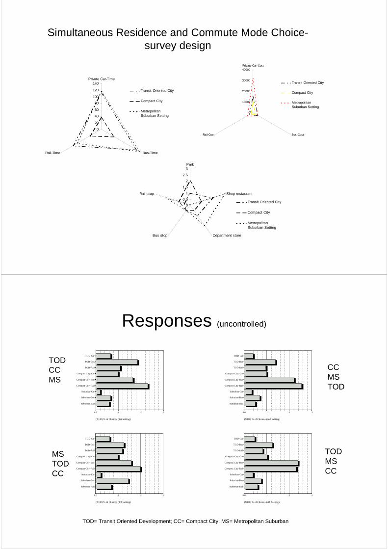
Simultaneous Residence and Commute Mode Choice-survey design

0

20

40

60

80

100

120

140Private Car-Time

Bus-TimeRail-Time

Transit Oriented City

Compact City

MetropolitanSuburban Setting

0

10000

20000

30000

40000Private Car-Cost

Bus-CostRail-Cost

Transit Oriented City

Compact City

MetropolitanSuburban Setting

0

0.5

1

1.5

2

2.5

3Park

Shop-restaurant

Department storeBus stop

Rail stop

Transit Oriented City

Compact City

MetropolitanSuburban Setting

Responses (uncontrolled)

TOD-Car

TOD-Bus

TOD-Rail

Compact City-Car

Compact City-Bus

Compact City-Rail

Suburban-Car

Suburban-Bus

Suburban-Rail

(X100) % of Choices (1st Setting)

.3.2.10.0

TOD-Car

TOD-Bus

TOD-Rail

Compact City-Car

Compact City-Bus

Compact City-Rail

Suburban-Car

Suburban-Bus

Suburban-Rail

(X100) % of Choices (2nd Setting)

.3.2.10.0

TOD-Car

TOD-Bus

TOD-Rail

Compact City-Car

Compact City-Bus

Compact City-Rail

Suburban-Car

Suburban-Bus

Suburban-Rail

(X100) % of Choices (3rd Setting)

.3.2.10.0

TODCCMS

CCMSTOD

MSTODCC

TODMSCC

TOD= Transit Oriented Development; CC= Compact City; MS= Metropolitan Suburban

TOD-Car

TOD-Bus

TOD-Rail

Compact City-Car

Compact City-Bus

Compact City-Rail

Suburban-Car

Suburban-Bus

Suburban-Rail

(X100) % of Choices (4th Setting)

.3.2.10.0

Responses (controlled by super districts-pooled)

DKI Jakarta

TOD-Car

TOD-Bus

TOD-Rail

Compact City-Car

Compact City-Bus

Compact City-Rail

Suburban-Car

Suburban-Bus

Suburban-Rail

Sum

140.0120.0100.080.060.040.020.00.0

Bekasi

TOD-Car

TOD-Bus

TOD-Rail

Compact City-Car

Compact City-Bus

Compact City-Rail

Suburban-Car

Suburban-Bus

Suburban-Rail

Sum

60.050.040.030.020.010.00.0

Bogor

TOD-Car

TOD-Bus

TOD-Rail

Compact City-Car

Compact City-Bus

Compact City-Rail

Suburban-Car

Suburban-Bus

Suburban-Rail

Sum

70.060.050.040.030.020.010.00.0

Tangerang

TOD-Car

TOD-Bus

TOD-Rail

Compact City-Car

Compact City-Bus

Compact City-Rail

Suburban-Car

Suburban-Bus

Suburban-Rail

Sum

50.040.030.020.010.0

Initial definition of DC models

• Models describe individual behaviour choosing a best option among discretealternatives.

• Decision maker – an individual person/a group of persons

• Alternatives– car, bus and railway

• Attributes– =attractiveness: travel cost, time

• Decision rule– dominance, lexicographic, utility

• Dependent variable: unobserved probability between 0 and 1

• Observation: individual choices which are either 0 or 1– Depart/arrive at a given time or not– Visit on a given destination or not– Use a given travel mode or not– Choose a given route or not

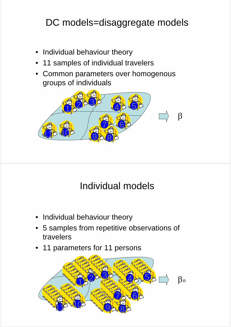
DC models=disaggregate models

1

1011 9 8

67

5432

• Individual behaviour theory

• 11 samples of individual travelers

• Common parameters over homogenous groups of individuals

β

Individual models

• Individual behaviour theory

• 5 samples from repetitive observations of travelers

• 11 parameters for 11 persons

βn1

1011 9 8

67

5432

Advantages

• calibrated by maximum likelihood estimation (MLE) rather than standard curve fitting (least squares)

• more stable (transferable) in time and space

• more efficient in data collection

• avoid ‘ecological correlation’

• more flexible representation of policy variables

Random utility theory

• Individuals belong to a homogeneous population

• Individuals act rationally and possess perfect information

i.e. They always select the option which maximizes their net personal utility subject to legal, social, physical and constraints.

• Individual’s choice set is predetermined

utility function

utility systematic error= +

systematic

error

observable variableseg.Individual SE characteristics

LOSs of alternatives constraint (omitted variables)

unobservable variableseg.Individual idiosyncrasies, taste, attitude,

habit, principle measurement errors of observable variables

Advanced Econometric Model

• Mixed (Random coefficients) Logit Model– Earlier applications by Boyd and Mellman (1980),

Cardell and Dunbar (1980) on automobile demand,– Customer-level data, such as Train et al. (1987) and

Ben-Akiva et al. (1993),– Lately, Bhat (1998) and Brownstone and Train (1999)

on cross-sectional data, and Erdem (1996), Revelt and Train (1998), and Bhat (2000) on panel data,

– A very general introduction by Train (1999),

– Does not show IIA property

– (but) Requires simulation

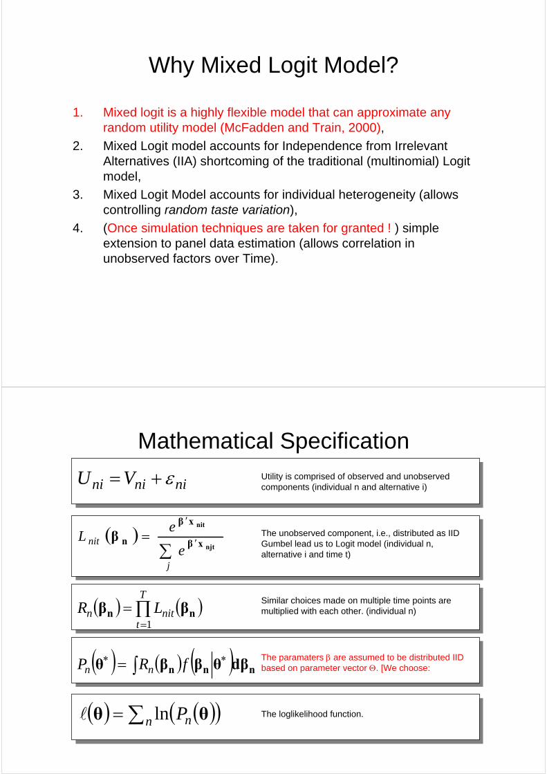
Why Mixed Logit Model?

1. Mixed logit is a highly flexible model that can approximate any random utility model (McFadden and Train, 2000),

2. Mixed Logit model accounts for Independence from Irrelevant Alternatives (IIA) shortcoming of the traditional (multinomial) Logit model,

3. Mixed Logit Model accounts for individual heterogeneity (allows controlling random taste variation),

4. (Once simulation techniques are taken for granted ! ) simple extension to panel data estimation (allows correlation in unobserved factors over Time).

Mathematical Specification

ninini VU ε+=

( )∑

′

′

=

j

nite

eL

njt

nit

xβ

xβ

nβ

( ) ( )∏=

=T

tnitn LR

1nn ββ

( ) ( ) ( ) nnn dβθββθ ∗∗ ∫= fRP nn

( ) ( )( )∑= n nP θθ lnl

Utility is comprised of observed and unobserved components (individual n and alternative i)

The unobserved component, i.e., distributed as IID Gumbel lead us to Logit model (individual n, alternative i and time t)

Similar choices made on multiple time points are multiplied with each other. (individual n)

The paramaters β are assumed to be distributed IID based on parameter vector Θ. [We choose:

The loglikelihood function.

Estimation

{random

random

1

ticdeterminis

11ni

K

niknkk

V

K

nikkini

K

niknkini xsxxU

ni

εσμαεβα +++=++= ∑∑∑4434421

44 844 76

44 344 21

∑∑+∑+

∑+∑+

=

j

xsx

xsx

nit K

njktnkk

K

njktkqj

K

niktnkk

K

niktkqi

e

eL

11

11

σμα

σμα

∏∑

∑+

∑+

=t

j

xsV

xsV

n K

njktnkknjt

K

niktnkknit

e

eR

1

1

σ

σ

( ) ( ) ( ) ( )nKnn

s

s

s

s

s

s t

j

xsV

xsV

n sdsdsd

e

eP

n

n

n

n

nK

nK

K

njktnkknjt

K

niktnkknit

Φ⋅⋅⋅ΦΦ⋅⋅⋅= ∫ ∫ ∫ ∏∑

∞=

−∞=

∞=

−∞=

∞=

−∞= ∑+

∑+

∗∗21

1

1

2

2 1

1

,σ

σ

σμ

( ) ( ) ( ) ( )∑ ∫ ∫ ∫ ∏∑

Φ⋅⋅⋅ΦΦ⋅⋅⋅=∞=

−∞=

∞=

−∞=

∞=

−∞= ∑+

∑+

nnKnn

s

s

s

s

s

s t

j

xsV

xsV

sdsdsd

e

en

n

n

n

nK

nK

K

njktnkknjt

K

niktnkknit

21

1

1

2

2 1

1

log,σ

σ

σμl

nkβ ( )kkN σμ ,~

nkkknk sσμβ +=

Estimation Results

0.008(0.05)-0.02(0.002)# of Household Members (relative to transit oriented development, car option i.e., the coefficient of this alternative is fixed to 0)

0.02(0.07)-0.03(0.01)Number of Four Wheeled Vehicles (relative to transit oriented development, car option i.e., the coefficient of this alternative is fixed to 0)

0.01(0.02)-0.01(0.01)Income (relative to transit oriented development, car option, i.e., the coefficient of this alternative is fixed to 0)

0.09(0.02)-0.02(0.01)Distance to Rail Station (relevant for Transit Oriented Development)

0.04(0.02)-0.02(0.007)Distance to Supermarkets (relevant for Transit Oriented Development and Compact City Development)

0.06(0.01)-0.02(0.01)Distance to Restaurants and Shops (relevant for Transit Oriented Development and Compact City Development)

0.04(0.02)-0.01(0.007)Distance to Park, Recreation etc. activities (relevant for Transit Oriented Development)

0.05(0.02)-0.02(0.009)Distance to CBD (relative to Transit Oriented Development)

0.02(0.06)-0.00 (0.00)Dummy Variable Transfers for Bus (relevant for Transit Oriented Development)

0.08(0.02)0.02 (0.01)Travel Time by mode (with respect to car)

0.05 (0.02)-0.04 (0.01)Travel Cost by mode (with respect to car)

--0.07 (0.01)Constant (with respect to Transit Oriented Development and Car)

Standard DeviationMeanVariable

Log Likelihood with only constant term=-2622.71Log Likelihood at convergence full model=-2577.45With respect to Log-likelihood Ratio Test (with 22 degrees of freedom), the model issignificant at a value lower than 0.005.Sample Size=303

ConclusionsIncrease of distance from relevant land uses affect residential choice such that if residential location is far away from relevant land uses individuals prefer to live in suburban setting. But if they are not far away, then the use of the public transit and its combination with accessibility to different land uses make household choose TOD and compact city environments.Travel cost when increased with respect to private car costs, household turn to private cars as their commuting mode of travel,But surprisingly travel time increase make people use transit option, which can only be explained by other psychological factors that are not captured by thecurrent model, e.g., the frustration that might be caused by staying behind the steering wheel and wait in the midst of the congested roads. This is supportive for an argument that automobile is the best option for a moderate ranges in time (also take this in distance)…

Further ResearchIn this study we have used simulation based on the normality of the parameter values; further research is needed on distributional assumptions of theparameters,The estimation is solely based on the stated intentions, the parameter values have to be weighted by the inclusion of the revealed preferences of the individuals. This requires the inclusion of the residential area properties of the households along with their actual living environments. The spatial separation of the sample is required with careful examination of the urban amenities.