Adaptation to Climate Change: Evidence fromUS Agriculture

Marshall Burke and Kyle Emerick∗

September 30, 2013

Abstract

Understanding the potential impacts of climate change on economic outcomes re-quires knowing how agents might adapt to a changing climate. We exploit large vari-ation in recent temperature and precipitation trends to identify adaptation to climatechange in US agriculture, and use this information to generate new estimates of thepotential impact of future climate change on agricultural outcomes. Longer-run adap-tations appear to have mitigated less than half – and more likely none – of the largenegative short-run impacts of extreme heat on productivity. Limited recent adaptationimplies substantial losses under future climate change in the absence of countervailinginvestments.

JEL codes: N5, O13, Q1, Q54Keywords: Climate change; adaptation; agriculture; climate impacts

∗Department of Agricultural and Resource Economics, University of California at Berkeley. Burke: mar-shall.burke@berkeley.edu. Emerick: kemerick@berkeley.edu. We thank Max Auffhammer, Peter Berck,Richard Hornbeck, Sol Hsiang, David Lobell, Wolfram Schlenker, and seminar participants at UC Berkeleyfor helpful comments and discussions. We thank Michael Roberts and Wolfram Schlenker for sharing data.All errors are our own.

1

1 Introduction

How quickly economic agents adjust to changes in their environment is a central question

in economics, and is consequential for policy design across many domains (Samuelson, 1947;

Viner, 1958; Davis and Weinstein, 2002; Cutler, Miller, and Norton, 2007; Hornbeck, 2012).

The question has been a theoretical focus since at least Samuelson (1947), but has gained

particular recent salience in the study of the economics of global climate change. Mounting

evidence that the global climate is changing (Meehl et al., 2007) has motivated a growing

body of work seeking to understand the likely impacts of these changes on economic outcomes

of interest. Because many of the key climatic changes will evolve on a time-scale of decades,

the key empirical challenge is in anticipating how economic agents will adjust in light of

these longer-run changes. If adjustment is large and rapid, and such adjustment limits the

resulting economic damages associated with climate change, then the role for public policy

in addressing climate change would appear limited. But if agents appear slow or unable to

adjust on their own, and economic damages under climate change appear likely to otherwise

be large, then this would suggest a much more substantial role for public policy in addressing

future climate threats.

To understand how agents might adapt to a changing climate, an ideal but impossible

experiment would observe two identical Earths, gradually change the climate on one, and

observe whether outcomes diverged between the two. Empirical approximations of this

experiment have typically either used cross-sectional variation to compare outcomes in hot

versus cold areas (e.g. Mendelsohn, Nordhaus, and Shaw (1994); Schlenker, Hanemann,

and Fisher (2005)), or have used variation over time to compare a given area’s outcomes

under hotter versus cooler conditions (e.g. Deschenes and Greenstone (2007); Schlenker

and Roberts (2009); Deschenes and Greenstone (2011); Dell, Jones, and Olken (2012)).

Due to omitted variables concerns in the cross-sectional approach, the recent literature has

preferred the latter panel approach, noting that while average climate could be correlated

with other time-invariant factors unobserved to the econometrician, short-run variation in

climate within a given area (typically termed “weather”) is plausibly random and thus better

identifies the effect of changes in climate variables on economic outcomes.

While using variation in weather helps to solve identification problems, it perhaps more

poorly approximates the ideal climate change experiment. In particular, if agents can adjust

in the long run in ways that are unavailable to them in the short run1, then impact estimates

derived from shorter-run responses to weather might overstate damages from longer-run

1e.g. Samuelson’s famed Le Chatelier principle, in which demand and supply elasticities are hypothesizedto be smaller in the short run than in the long run due to fixed cost constraints.

2

changes in climate. Alternatively, there could be short-run responses to inclement weather,

such as pumping groundwater for irrigation in a drought year, that are not tenable in the

long-run if the underlying resource is depletable (Fisher et al., 2012). Thus it is difficult

to even sign the “bias” implicit in estimates of impacts derived from short-run responses to

weather.

In this paper we exploit variation in longer-term changes in temperature and precipitation

across the US to identify the effect of climate change on agricultural productivity, and to

quantify whether longer-run adjustment to changes in climate has indeed exceeded shorter-

run adjustment. Recent changes in climate have been large and vary substantially over

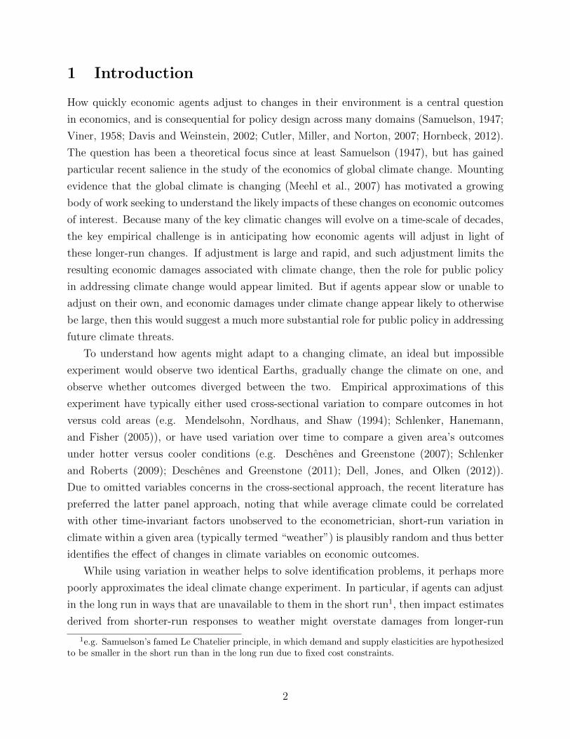
space: as shown in Figure 1, temperatures in some counties fell by 0.5◦C between 1980-2000

while rising 1.5◦C in other counties, and precipitation across counties has fallen or risen by

as much as 40% over the same period. We adopt a “long differences” approach and model

county-level changes in agricultural outcomes over time as a function of these changes in

temperature and precipitation, accounting for time-invariant unobservables at the county

level and time-trending unobservables at the state level.

This approach offers three distinct advantages over existing work. First, unlike either the

panel or cross-sectional approaches, it closely replicates the idealized climate change impact

experiment, quantifying how farmer behavior responds to longer-run changes in climate while

avoiding concerns about omitted variables bias. Second, observed variation in these recent

climate changes largely spans the range of projected near-term changes in temperature and

precipitation provided by global climate models, allowing us to make projections of future

climate change impacts that do not rely on large out-of-sample extrapolations. Finally, by

comparing how outcomes respond to longer-run changes in climate to how they respond to

shorter run fluctuations as estimated in the typical panel model, we can test whether the

shorter-run damages of climatic variation on agricultural outcomes are in fact mitigated in

the longer-run. Quantifying this extent of recent climate adaptation in agriculture is of both

academic and policy interest, and a topic about which there exists little direct evidence.

We find that productivity of the primary US field crops, corn and soy, is substantially

affected by these long-run trends in climate. Our main estimate for corn suggests that

spending a single day at 30◦C (86◦F) instead of the optimal 29◦C reduces yields at the end

of the season by about half a percent, which is a large effect.2 The magnitude of this effect

is net of any adaptations made by farmers over the 20 year estimation period, and is robust

to using different time periods and differencing lengths.

To quantify the magnitude of any yield-stabilizing adaptations that have occurred, we

2The within-county standard deviation of days of exposure to “extreme” temperatures above 29◦C is 30,meaning a 1SD increase in exposure would reduce yields by 15%.

3

then compare these long differences estimates to panel estimates of short-run responses to

weather. Long run adaptations appear to have mitigated less than about half of the short-

run effects of extreme heat exposure on corn yields, and point estimates across a range of

specifications suggest that long run adaptions have more likely offset none of these short

run impacts. We also show limited evidence for adaptation along other margins within

agriculture: revenues are similarly harmed by extreme heat exposure, and farmers do not

appear to be substantially altering the inputs they use nor the crops they grow in response

to a changing climate.

We then examine different explanations for why adjustment to recent climate change has

been minimal. For instance, adaptation could be limited because there are few adjustment

opportunities to exploit, or alternatively because farmers don’t recognize that climate has in

fact changed and that adaptation is needed. Which it is is important for how we interpret

our results, and in particular how they extrapolate to future warming scenarios. If farmers

failed to adapt in the past because they did not recognize the climate was changing, but in

the future they become aware of these changes and quickly adapt, then our findings would

be a poor guide to future impacts of warming. On the other hand, if farmers had recognized

the need for adaptation but were unable to do so, then their past responses to extreme heat

exposure would provide a plausible “business-as-usual” benchmark for the impacts of future

warming in the absence of novel investment in adaptation.

While we cannot directly observe farmer perceptions of climate change, there is both

theoretical and empirical guidance on which locations should be more likely to have learned

about the negative effects of extreme heat or to have recognized that the climate was chang-

ing: locations that faced larger exposure to extreme heat in an earlier period, locations where

the underlying temperature variance is lower (making any warming “signal” stronger), loca-

tions with better educated farmers, or locations where voting behavior suggest that a belief

in climate change is more likely. We find no evidence that farmers in such areas responded

any differently to extreme heat exposure than farmers previously un-exposed, less educated,

or in more climate-change-skeptical regions, providing some evidence that adaptation was

not limited by a failure of recognition.

As a final exercise, we combine our long differences estimates with output from 18 global

climate models to project the impacts of future climate change on the productivity of corn,

a crop increasingly intertwined with the global food and fuel economy. Such projections are

an important input to climate policy discussions, but bear the obvious caveat that future

adjustment capabilities are constrained to what farmers were capable of in the recent past.

Nevertheless, because our projections are less dependent on large out-of-sample extrapola-

tion, and because they account for farmers’ recent ability to adapt to longer-run changes

4

in climate, we believe they are a substantial improvement over existing approaches. Our

median estimate is that corn yields will be about 15% lower by mid-century relative to a

world without climate change, with some climate models projecting losses as low as 7% and

others as high as 64%. Valued at current prices and production quantities, this fall in corn

productivity in our sample counties would generate annual losses of $6.7 billion dollars by

2050. We note that a 15% yield loss is on par with expected yield losses resulting from the

well-publicized “extreme” drought and heat wave that struck the US midwest in the summer

of 2012. Given the substantial role that corn plays in US agricultural production and the

dominant role that the US plays in the global trade of corn, these results imply substantial

global damages if the more negative outcomes in this range are realized.

Our work contributes to the rapidly growing literature on climate impacts, and in par-

ticular to a host of recent work examining the potential impacts of climate change on US

agriculture (Mendelsohn, Nordhaus, and Shaw, 1994; Schlenker, Hanemann, and Fisher,

2005; Deschenes and Greenstone, 2007; Schlenker and Roberts, 2009; Fisher et al., 2012).

We build on this work by directly quantifying how farmers have responded to longer-run

changes in climate, and are able to construct projections of future climate impacts that

account for this observed ability to adjust.

Methodologically our work is closest to Dell, Jones, and Olken (2012) and to Lobell

and Asner (2003). Dell, Jones, and Olken (2012) focus on panel estimates of the impacts

of country-level temperature variation on economic growth, but also use cross-country dif-

ferences in recent warming to estimate whether there has been “medium-run” adaptation.

Their point estimates suggest little difference between responses to short-run fluctuations

and medium-run warming, but estimates for the latter are imprecise and not always signif-

icantly different from zero, meaning that large adaptation cannot be ruled out. Lobell and

Asner (2003) study the effect of trends in average temperature on trends in US crop yields,

finding that warmer average temperatures are correlated with declining yields. We build on

this work by providing more precise estimates of recent adaptation, and by accounting more

fully for time-trending unobservables that might otherwise bias estimates.

Our findings also relate to a broader literature on long-run economic adjustments. A body

of historical research suggests that economic productivity often substantially recovers in the

longer run after an initial negative shock (Davis and Weinstein, 2002; Miguel and Roland,

2011), and that in the long run farmers in particular are able to exploit conditions that

originally appeared hostile (Olmstead and Rhode, 2011). Somewhat in contrast, Hornbeck

(2012) exploits variation in soil erosion during the 1930’s American Dust Bowl to show that

negative environmental shocks can have substantial and lasting effects on productivity. Using

data from a more recent period, we examine responsiveness to a slower-moving environmental

5

“shock” that is very representative of what future climate change will likely bring. Similar

to Hornbeck, we find limited evidence that agricultural productivity has adapted to these

environmental changes, with fairly negative implications for the future impacts of climate

change on the agricultural sector.

The remainder of this paper is organized as follows. In Section 2 we develop a simple

model of farmer adaptation and use it to motivate our estimation approach. Section 3

describes our main results on the extent of past adaptation. In Section 4 we try to rule out

alternative explanations for our results. Section 5 uses data from global climate models to

build projections of future yield impacts, and Section 6 concludes and discusses implications

for policy.

2 Model and Empirical Approach

Agriculture is a key sector where future climate change is estimated to have large detrimental

effects, and is a primary focus of the empirical literature on climate change impacts. To

formalize the ways in which our identification of climate impacts differs from that of the past

literature, we develop a simple model of farmer adaptation, building on earlier work by Kelly,

Kolstad, and Mitchell (2005). The climate literature generally understands adaptation as any

adjustment to a changing environment that exploits beneficial opportunities or moderates

negative impacts.3 Adaptation thus requires an agent to recognize that something in her

environment has changed, to believe that an alternative course of action is now preferable

to her current course, and to have the capability to implement that alternative course.

We consider a farmer facing a choice about which of two crop varieties to grow, where

one performs relatively better in cooler climates (variety 1) and the other in warmer climates

(variety 2). We assume this relative performance is known to the farmer. Denote the choice

of variety for farmer i as xit ∈ {0, 1}, with xit = 1 the choice to grow the relatively heat-

tolerant variety 2. The output of farmer i in period t is yit = f(xit, zit), where zit is realized

temperature in period t and is drawn from a normal distribution ∼ N(ωt, σ2). We assume a

quadratic overall production technology with respect to temperature:

yit = β0 + β1zit + β2z2it + xit(α0 + α1zit + α2z

2it) (1)

with production for the conventional variety given by β0 + β1zit + β2z2it, and the differential

productivity between the conventional and heat-tolerant varieties given by α0 +α1zit +α2z2it.

The farmer in year i chooses xit to maximize expected output prior to realizing weather.

3See Zilberman, Zhao, and Heiman (2012) and Burke and Lobell (2010) for an overview.

6

The heat-tolerant crop will be chosen if E(α0 +α1zit +α2z2it) > 0, which can be rewritten as

α0 + α1ωt + α2(ω2t + σ2) > 0. (2)

We assume that the α and β parameters are known to the farmer but not to the econome-

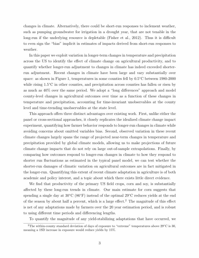
trician. Figure 2 displays the productivity of the two varieties as a function of temperature.

As drawn, the productivity frontiers have similar concavity4 (α2 ≈ 0) such that the perfectly

informed farmer adopts the heat-tolerant crop when the expected temperature exceeds ω.

We incorporate climate change as a shift in mean temperature from ω → ω′, with

ω < ω < ω′. In keeping with evidence from climate science (see Meehl et al. (2007)),

we assume that this increase in mean is not accompanied by a change in variance, such

that after climate change the farmer experiences zit ∼ N(ω′, σ2) in each year. A fully in-

formed farmer recognizes this change and immediately adopts the heat-tolerant crop, which

we consider “adaptation”. In reality, farmers likely learn about changes in climate over

time and only adjust behavior after acquiring strong enough information that climate has

changed. Following Kelly, Kolstad, and Mitchell (2005), we assume this learning follows a

simple Bayesian process where the farmer has an prior belief about ωt but knows that this

belief is imperfect. We denote the belief as µt and its variance as 1/τt, such that in period t

the farmer believes ω ∼ N(µt, 1/τt). In each period she observes zit and updates her belief

about the average temperature to µt+1 using a weighted combination of her prior belief and

the new climate realization she experiences. Letting ρ = 1/σ2, the farmer’s belief about

mean climate after T years is given by (DeGroot, 1970):

µT =τtµt + Tρzitτt + Tρ

(3)

With τt+1 = τt + ρ, then in expectation it follows that:

µT − ω′ =τ0(µ0 − ω′)τ0 + Tρ

(4)

Equation (4) has two important implications: beliefs about mean temperature converge to

the true value as the number of time periods increases (T ↑), and converge more quickly

when there is less variance in annual temperature (i.e. when ρ is larger). This suggests

4A negative value of α2 would indicate that productivity of the heat-tolerant crop is more response totemperature changes (i.e. the productivity or profit frontier for the heat-tolerant crop is “more concave”). Inthis case, if climate variability is large, then the expected gain from adaptation at average climate must belarge enough to offset expected losses in bad years. With α2 > 0, the response function for the heat tolerantcrop is “flatter” such that the farmer is willing to adopt the heat tolerant crop before the intersection of thetwo curves because of the increased certainty that it provides.

7

that farmers should be more likely to recognize changes in climate – and thus adapt to

those changes, if information is a constraint to adaptation – in areas where the temperature

variance is low, and when they are given more time to observe realizations of the new climate.

We use these predictions to help us interpret our main findings in what follows.

2.1 Existing approaches

Returning to Figure 2, the long-term damages imposed by a shift in climate will be v0 − v1if adaptation takes place.5 Past literature has taken two approaches to estimating this

quantity. In pioneering work, Mendelsohn, Nordhaus, and Shaw (1994) use cross-sectional

variation in average temperature and precipitation (and their squares) to explain variation

in agricultural outcomes across US counties. The cross sectional specification is

yi = α + β1wi + β2w2i + ci + εi, (5)

where yi is some outcome of interest in county i, wi is again the average temperature, and

ci other time invariant factors affecting outcomes (such as soil quality). Mendelsohn et al’s

preferred dependent variable is land values, which represent the present discounted value of

the future stream of profits that could be generated with a given parcel of land, and thus in

principle embody any possible long-run adaptation to average climate. Therefore, a county

with average temperature of ω will achieve v0 on average, a county with average temperature

of ω′ will achieve v1, and the estimates of β1 and β2 along with a projected rise in average

temperatures from ω to ω′ would seem to identify the desired quantity of v0 − v1.Cross sectional models in this setting make an oft-criticized assumption: that average

climate is not correlated with other unobserved factors (the ci – soil quality, labor productiv-

ity, technology availability etc) that also affect outcomes of interest (Schlenker, Hanemann,

and Fisher, 2005; Deschenes and Greenstone, 2007). Given these omitted variables concerns,

more recent work has used panel data to explore the relationship between agricultural out-

comes and variation in temperature and precipitation (Deschenes and Greenstone (2007);

Schlenker and Roberts (2009); Welch et al. (2010); Lobell, Schlenker, and Costa-Roberts

(2011)).6 The data generating process in this approach is:

yit = α + β1zit + β2z2it + ci + εit (6)

5Kelly, Kolstad, and Mitchell (2005) call this the “equilibrium response”, in contrast to the costs incurredwhen undertaking adaptation (e.g. the purchase of a more expensive heat-tolerant variety), which they term“adjustment costs”.

6Examples in the climate literature outside of agriculture include Burke et al. (2009); Deschenes andGreenstone (2011); Auffhammer and Aroonruengsawat (2011); Dell, Jones, and Olken (2012).

8

All time invariant factors are absorbed by the location fixed effects ci, and impacts of tem-

perature and precipitation on (typically annual) outcomes are thus identified from deviations

from location-specific means.7 Because this year-to-year variation in temperature and pre-

cipitation (typically termed “weather”) is plausibly exogenous, fixed effects regressions over-

come omitted variables concerns with cross-sectional models, and the effect of temperature

on outcomes such as yield or profits can be interpreted causally.

Many studies then combine the estimated short-run responses from panel regressions with

output from global climate models to project potential impacts under future climate change.8

In making these projections, the implicit assumption is again that short-run responses to

variation in weather are representative of how farmers will respond to longer-run changes

in average climate. It is not obvious this will be the case. Consider a panel covering many

years, with a temperature rise from ω to ω′ occuring somewhere within these years. The

panel model would identify movement along either one of the two curves shown in Figure

2, with the point estimate being a weighted average of the slopes of the two curves, with

weights depending on if and when the varietal switch occurred. If the heat-tolerant crop

is adopted at the end of the period then fixed effects estimates will be heavily weighted

towards the curve for the conventional crop, overstating equilibrium losses. If adaptation

is instantaneous then fixed effects estimates trace out the curve for the heat-tolerant crop,

which could understate impacts if (as drawn) the slope of the response function is positive

at ω′. Thus estimates of short-run responses to weather will not even bound estimates of

longer-run response to climate. Panel models therefore solve identification problems in the

cross-sectional approach, at the cost of more poorly approximating the idealized climate

change experiment.

2.2 The long differences approach

We attempt to simultaneously overcome the limitations of both the cross-sectional and panel

approaches by long differencing. We use (6) to construct longer run yield and temperature

7McIntosh and Schlenker (2006) show that including a quadratic term in the standard panel fixed effectsmodel allows unit means to re-enter the estimation. Inclusion of a squared term therefore results in impactsof the independent variable of interest being derived not only from within-unit variation over time but alsofrom between-unit variation in means. In principle, this would allow for estimation of the outer as well asthe inner envelope, a strategy explored by Schlenker (2006), although it is not clear that omitted variablesconcerns have not also re-entered the estimation along with the unit means. In any case, growing degree daysallow temperature to enter non-linearly without the complication of the quadratic term, and we exploit thisfact to generate estimates of adaptation. Furthermore, using trends in climate to identify climate sensitivitiesremains an arguably more “direct” approach to understanding near-term impacts of future climate change,and is thus the approach we take here.

8See Burke et al. (2013) for a review of these studies and for the use of global climate models in thiscontext.

9

averages at two different points in time for a given location, and calculate changes in average

yields as a function of changes in average temperature. Consider two multi-year periods

denoted “a” and “b”, each spanning n years. Our approach is to separately sum (6) over all

the years in each period, e.g. with the average yield in period a given by yia = 1n

∑t∈a yit

and average temperature zia representing the averaged zit’s over the same period. Equation

(6) for period a becomes:

yia = α + β1zia + β2zia2 + ci + εia. (7)

Defining period b similarly, we can “long difference” over the two periods to get:

yib − yia = β1(zib − zia) + β2(zib2 − zia2) + (ci − ci) + (εib − εia) (8)

The time-invariant factors drop out, and we can rewrite as:

∆yi = β1∆zi + β2∆(zi)2 + ∆εi, (9)

Generating unbiased estimates of β1 and β2 requires that changes in temperature between

the two periods are not correlated with time-varying unobservables that also affect outcomes

of interest. Below we provide evidence that differential climate trends across our sample of

US counties are likely exogenous and surprisingly large.

Estimating the impact of climate on agricultural productivity with the long differences

approach in (9) offers substantial advantages over both the cross-sectional and panel ap-

proaches. First, it arguably better approximates the ideal “parallel worlds” experiment.

That experiment randomly assigns climate trends to different earths, and the long differ-

ences approximation utilizes variation in longer-run climate change that are unlikely to be

correlated with variables that explain changes in yield. Second, unlike the cross-sectional

approach, the long differences estimates are immune to time-invariant omitted variables, and

unlike the panel approach the relationship between climate and agricultural productivity is

estimated from long-term changes in average conditions instead of short-run year-to-year

variation. Finally, because long differences estimates will embody any adaptations that

farmers have undertaken to recent trends, and because the range in these trends falls within

the range of projected climate change over at least the next three decades, then projections

of future climate change impacts on agricultural productivity based on long differences es-

timates would appear more trustworthy than those based on either panel or cross-sectional

methods.

We then use this strategy to quantify the extent of recent adaptation in US agriculture,

10

comparing our long differences estimates to those from an annual panel model. We would

interpret more positive long difference estimates as evidence of adaptation: that farmers are

better able to adjust to longer-run changes in climate than they are to shorter-run changes

in weather. In Figure 2, if any adaptation takes place, the long differences approach should

identify v0−v1. If no adaptation occurs, then long difference regressions will identify v0−v2,i.e. the same damages identified by fixed effects. We attempt to rule out other explanations

for divergence between panel and long-differences estimates - e.g. measurement error, or

adaptation outside of agriculture - in Section 4.

2.3 Data and estimation

Our agricultural data come from the United States Department of Agriculture’s National

Agricultural Statistics Service. Crop area and yield data are available at the county-year

level, and economic measures of productivity such as total revenues and agricultural land

values are available every five years when the Agricultural Census is conducted.9 Our unit

of observation is thus the county, and in keeping with the literature we focus the main

part of the analysis on counties that are east of the 100th meridian. The reason for this is

that cropland in the American West typically relies on highly subsidized irrigation systems,

and the degree of adaptation embodied in the use and expansion of these systems might

poorly extrapolate to future scenarios as the federal government is unlikely to subsidize new

water projects as extensively as it has in the past (Schlenker, Hanemann, and Fisher, 2005).

Over the last decade, the counties east of the 100th meridian accounted for 93% of US corn

production and 99% of US soy production.

Our climate data are from Schlenker and Roberts (2009) and consist of daily interpolated

values of precipitation totals and maximum and minimum temperatures for 4 km grid cells

covering the entire United States over the period 1950-2005. These data are aggregated to

the county-day level by averaging daily values over the grid cells in each county where crops

are grown, as estimated from satellite data.10

Past literature has demonstrated strong non-linearities in the relationship between tem-

perature and agricultural outcomes (e.g. Schlenker and Roberts (2009)). Such non-linearities

are generally captured using the concept of growing degree days (GDD). GDD measure the

amount of time a crop is exposed to temperatures between a given lower and upper bound,

with daily exposures summed over the growing season to get a measure of annual growing

degree days. Denoting the lower bound as tl and the upper bound as th, if td is the average

temperature on a given day d, then degree days for that day are calculated as:

9We thank Michael Roberts for sharing additional census data that are not yet archived online.10We thank Wolfram Schlenker for sharing the weather data and the code to process them.

11

GDDd;tl:th =

0 if td ≤ tl

td − tl if tl < td ≤ th

th − tl if th < td

Daily degree days are then summed over all the days in the growing season (typical April 1

to September 30th for corn in the United States) to get an annual measure of GDD.

Using this notion of GDD, and using the county agricultural data described above, we

model agricultural outcomes as a simple piecewise linear function of temperature and pre-

cipitation.11 We estimate the long differences model:

∆yis = β1∆GDDis;l0:l1 +β2∆GDDis;l1:∞+β3∆Precis;p<p0 +β4∆Precis;p>p0 +αs+∆εis, (10)

where ∆yis is the change in some outcome y in county i in state s between two periods. In

our main specification these two periods are 1980 and 2000, and we calculate endpoints as

5-year averages to more effectively capture the change in average climate or outcomes over

time. That is, for the 1980-2000 period we take averages for each variable over 1978-1982

and over 1998-2002, and difference these two averages.

The lower temperature “piece” in (10) is the sum of GDD between the bounds l0 and l1,

and ∆GDDis;l0:l1 term gives the change in GDD between these bounds over the two periods.

The upper temperature “piece” has a lower bound of l1 and is unbounded at the upper end,

and the ∆GDDis;l1:∞ term measures the change in these GDD between the two periods.12 We

also measure precipitation in a county as a piecewise linear function with a kink at p0. The

variable Precis;p<p0 is therefore the difference between precipitation and p0 interacted with

an indicator variable for precipitation being below the threshold p0. Precis;p>p0 is similarly

defined for precipitation above the threshold.13 In the estimation we set l0 = 0 and allow the

data to determine l1 and p0 by looping over all possible thresholds and selecting the model

11We choose the piecewise linear approach for two reasons. First, existing work on US agricultural responseto climate suggests that a simple piecewise linear function delivers results very similar to those estimatedwith much more complicated functional forms (Schlenker and Roberts, 2009). Second, these other functionalforms typically feature higher order terms, which in a panel setting means that unit-specific means re-enterthe estimation (McIntosh and Schlenker, 2006). This not only raises omitted variables concerns, but itcomplicates our strategy for estimating the extent of past adaptation by comparing long differences withpanel estimates; in essence, identification in the panel models in no longer limited to location-specific variationover time.

12As an example, if l0 = 0 and l0 = 30, then a given set of observed temperatures -1, 0, 1, 10, 29, 31, and35 would result in GDDis;l0:l1 equal to 0, 0, 1, 10, 29, 30, and 30, and GDDis;l1:∞ equal to 0, 0, 0, 0, 1, and5.

13A simple example is useful to illustrate the differencing of precipitation variables when the threshold iscrossed between periods. Consider a county with an increase in average precipitation from 35 mm in 1980to 50 mm in 2000. If the precipitation threshold is 40 mm, then ∆Precis;p<p0

= 5 and ∆Precis;p>p0= 10.

12

with the lowest sum of squared residuals.

Importantly, we also include in (10) a state fixed effect αs which controls for any un-

observed state-level trends. This means that identification comes only from within-state

variation, eliminating any concerns of time-trending unobservables at the state level. Fi-

nally, to quantify the extent of recent adaptation, we estimate a panel version of (10), where

observations are at the county-year level and the regression includes county and year fixed

effects. As suggested by earlier studies (e.g. Schlenker and Roberts (2009)), the key co-

efficient in both models is likely to be β2, which measures how corn yields are affected by

exposure to extreme heat. If farmers adapt significantly to climate change then we would

expect the coefficient β2 to be significantly larger in absolute value when estimated with

panel fixed effects as compared to our long differences approach. The value 1 − βLD2 /βFE

2 ,

gives the percentage of the negative short-run impact that is offset in the longer run, and is

our measure of adaptation to extreme heat.

Figure 1 displays the variation that is used in our identification strategy. Some US coun-

ties have cooled slightly over the past 3 decades, while others have experienced warming

equivalent to over 1.5 times the standard deviation of local temperature. Differential trends

in precipitation over the 1980-2000 have been similarly large, with precipitation decreasing

by more than 30% in some counties and increasing by 30% in others. By way of comparison,

the upper end of the range in these recent temperature trends is roughly equivalent to the

mean warming projected by global climate models to occur over US corn area by 2030, and

the range in precipitation trends almost fully contains the range in climate model projections

of future precipitation change over the same area by the mid-21st century. More importantly,

substantial variation is apparent within states. For instance, Lee County in the southeastern

Iowa experienced an increase in average daily temperature during the main corn growing

season of 0.46◦C, and Mahaska county – approximately 80 miles to the northwest – expe-

rienced a decrease in temperature of 0.3◦C over the same period. Corn yields in parts of

northern Kentucky declined slightly while rising by 20-30% only 100 miles to the south.

While we explore robustness of our results to different time periods and differencing

lengths, we focus on the post-1980 period for a number of reasons. First, warming trends

since 1980 were much larger than in earlier periods. For instance, over the 1960-1980 period,

only half of the counties in our sample experienced average warming, and none experience

warming of more than 1C (see Figure A.7). Second, recognition of climate change was much

higher in this later period, which helps alleviate some concerns that a lack of recognition of

climate change is what is driving our results. In particular, prior to 1980 there was even

significant scientific and popular concern about the risks from “global cooling” (e.g. Gwynne

(1975)), and only during the 1980’s and 1990’s was there growing recognition that the climate

13

was warming and that increasing greenhouse gas emissions meant there would very likely be

further warming in the future.

Section A.1 in the Appendix more rigorously quantifies the variation in temperature used

in the long differences estimation. We document that observed temperature changes over the

period do in fact represent meaningful long-run changes rather than just short-run variation

around endpoint years, and we show that the residual variation in these temperature changes

remains large (relative to projected future changes) after accounting for state fixed effects.

2.4 Are recent climate trends exogenous?

There are a few potential violations to the identifying assumption in (10). The first is that

trends in local emissions could affect both climate and agricultural outcomes. In particular,

although greenhouse gases such as carbon dioxide typically become “well mixed” in the

atmosphere soon after they are emitted, other species such as aerosols are taken out of the

atmosphere by precipitation on a time scale of days, meaning that any effect they have

will be local. Aerosols both decrease the amount of incoming solar radiation, which cools

surface temperatures and lowers soil evaporation, and they tend to increase cloud formation,

although it is somewhat ambiguous whether this leads to an increase in precipitation. For

instance, Leibensperger et al. (2011) found that peak aerosol emissions in the US during the

1970s and 1980s reduced surface temperatures over the central and Mid-Atlantic US by up

to 1oC, and led to modest increases in precipitation over the same region.

The effect of aerosols on crops is less well understood (Auffhammer, Ramanathan, and

Vincent, 2006). While any indirect effect through temperature or precipitation will already

be picked up in the data, aerosols become an omitted variables concern if their other in-

fluence on crops – namely their effect on solar radiation – have important effects on crop

productivity. Because crop productivity is generally thought to be increasing and concave in

solar radiation, reductions in solar radiation are likely to be harmful, particularly to C4 pho-

tosynthesis plants like corn that do not become light saturated under typical conditions.14

However, aerosols also increase the “diffuse” portion of light (think of the relatively even

light on a cloudy day), which allows additional light to reach below the canopy, increasing

productivity. A recent modeling study finds negative net effects for corn, with aerosol con-

centrations (circa the year 2000) reducing corn yields over the US midwest by about 10%,

albeit with relatively large error bars. This would make it likely that, if anything, aerosols

14Crops that photosynthesize via the C3 pathway, which include wheat, rice, and soybeans, become ”lightsaturated” at one-third to one-half of natural sunlight, meaning that reductions in solar radiation above thatthreshold would have minimal effects on productivity. C4 plants such as corn do not light saturate undernormal sunlight, so are immediately harmed by reductions in solar radiation (Greenwald et al. (2006)).

14

will cause us to understate any negative effect of warming on crop yields: aerosols lead to

both cooling (which is generally beneficial in our sample) and to a reduction in solar radia-

tion (which on net appears harmful for corn). In any case, the inclusion of state fixed effects

means that we would need significant within-state variation in aerosol emissions for this to

be a concern.

The second main omitted variables concern is changes in local land use. Evidence from

the physical sciences suggests that conversion between types of land (e.g. conversion of

forest to pasture, or pasture to cropland), or changes in management practices within pre-

existing farmland (e.g. expansion of irrigation) can have significant effects on local climate.

For instance, expansion in irrigation has been shown to cause local cooling (Lobell, Bala,

and Duffy, 2006), which would increase yields both directly (by reducing water stress) and

indirectly (via cooling), leading to a potential omitted variables problem. The main empirical

difficulty is that local land use change could also be an adaptation to changing climate – i.e.

a consequence of a changing climate as well as a cause. In the case of irrigation, adaptation

and irrigation-induced climate change are likely to go in opposite directions: if irrigation is an

omitted variable problem, we would need to see greater irrigation expansion in cooler areas,

whereas if irrigation is an adaptation, we would expect relatively more expansion in warm

areas. Overall, though, because we see little change in either land area or land management

practices, we believe these omitted variables concerns to be limited as well.

The most recent evidence from the physical sciences suggests that the large differential

warming trends observed over the US over the past few decades are likely due to natural

climate variability - in particular, to variation in ocean temperatures and their consequent

effect on climate over land (e.g. Meehl, Arblaster, and Branstator (forthcoming)). As such,

these trends appear to represent a true “natural experiment”, and are likely exogenous with

respect to the outcomes we wish to measure. Nevertheless, as a final check on exogeneity,

we show in Table A.2 that the within-state change in exposure to extreme heat during the

1980-2000 period are not strongly correlated with several county-level covariates.

3 Empirical Results

Our primary analysis focuses on the effect of longer-run changes in climate on the produc-

tivity of corn and soy, the two most important crops in the US in terms of both area sown

and production value. The yield (production per acre) of these two crops is the most ba-

sic measure of agricultural productivity, and is well measured annually at the county level.

However, because a focus on yields alone will not cover the full suite of adaptations that

farmers might have employed, we will examine adjustments along other possible margins.

15

3.1 Corn productivity

The results from our main specifications for corn yields are given in Table 1 and shown

graphically in Figure 3. In our piecewise linear approach, productivity is expected to increase

linearly up to an endogenous threshold and then decrease linearly above that threshold, and

the long differences and panel models reassuringly deliver very similar temperature thresholds

(29◦C and 28◦C, respectively) and precipitation thresholds (42cm and 50cm). In Columns

1-3 we run both models under the thresholds selected by the long differences, and in Columns

4-6 we fix thresholds at values chosen by the panel.

The panel and long differences models deliver very similar estimates of the responsiveness

of corn yields to temperature. Exposure to GDD below 29◦C (row 1) have small and generally

insignificant effects on yields, but increases in exposure of corn to temperatures above 29◦

result in sharp declines in yields, as is seen in the second row of the table and in Figure 3.

In our most conservative specification with state fixed effects, exposure to each additional

degree-day of heat above 29◦C results in a decrease in overall corn yield of 0.44%.15 The

panel model delivers a slightly more negative point estimate, a -0.56% yield decline for every

one degree increase above 29◦C, but (as quantified below) we cannot reject that the estimates

are the same. We obtain similar results when the two models are run under the temperature

and precipitation thresholds chosen by the panel model (Columns 4-6).

The estimates of the effects of precipitation on corn productivity are somewhat more

variable. The piecewise linear approach selected precipitation thresholds at 42 cm (long

differences) or 50 cm (panel), but most of the variation in precipitation is at values above 42

cm – e.g. the 10th percentile of annual county precipitation is 41.3 cm. Long differences point

estimates suggest an approximate increase in yields of 0.33% for each additional centimeter

of rainfall above 42 cm, which are of the opposite sign and substantially larger than panel

estimates. Nevertheless, we note that even the long differences precipitation estimates remain

quite small relative to temperature effects: on a growing season precipitation sample mean of

57cm, a 20% decrease (roughly the most negative climate model projection for US corn area

by the end of century) would reduce overall yields by less than 4%. As we show in Section

5, and consistent with other recent findings (Schlenker and Roberts, 2009; Schlenker and

15While we prefer the more conservative specifications with state fixed effects in Table 1, one concern withthe inclusion of state fixed effects is that farmer responses to increasing temperature might vary meaningfullyat the state level, for instance if governments in states that experienced substantial warming helped theirfarmers invest in adaptation measures. These policies would be absorbed by the state fixed effects, andcould obscure meaningful adaptation measures undertaken by farmers. Our results appear inconsistent witha story of state-level adaptation to extreme heat. The effects of extreme heat in the specifications withoutstate fixed effects (columns 1 and 4) are substantially more negative than in the comparable specificationswith state fixed effects, which is the opposite of what would be expected if state-level adaptation policieswere an omitted variable in these regressions.

16

Lobell, 2010), any future impacts of climate change via changes in precipitation are likely to

be dominated by changes in yields induced by increased exposure to extreme heat.

To test robustness of the corn results, we show in the remainder of this subsection that our

results are relatively insensitive to the choice of endpoint years, to the number of years used

to calculate endpoints, and to an alternate estimation strategy which further weakens our

identification assumptions. In Appendix A.3, we provide further evidence that our results

are insensitive to the exclusion of yield and temperature outliers, and to the inclusion of

baseline covariates in the regression.

We first show that our results are largely unchanged when we change the time period

under study. In particular, we estimate Equation (10) varying T0 from 1955 to 1995 in 5

year increments, and for each value of T0 we estimate 5, 10, 15, 20, 25, and 30 year difference

models.16 Results are shown graphically in Figure 4. We display the difference between the

estimate of β2 for 1980-2000 (our baseline estimate) and the estimate of β2 for the period

determined by the starting year and differencing length. The 95% confidence intervals of the

differences are calculated by bootstrapping.17 The average estimate of β2 across these 39

models is -0.0058, with only 8 of the estimates of β2 being statistically different from our main

1980-2000 estimate and none statistically different in the positive direction. This suggests if

anything that our baseline point estimate on the effect of extreme heat is conservative.18 We

conduct an analogous exercise for the panel model to make sure that the effect of extreme

heat in the panel does not vary with the chosen time period. Results are plotted in Figure

A.8, and agree with earlier findings in Schlenker and Roberts (2009) that the effects of

inter-annual deviations in extreme heat have not declined significantly over time.19

16Some models of course could not be estimated since our data end at 2005, meaning our 5-year smoothedestimates are only available through 2003. In each model we limit the sample to the set of counties fromTable 1. Each regression is weighted by 5 year average corn area during the starting year. The temperatureand precipitation thresholds are fixed at 29◦ and 42 cm across models.

17We drew 1000 samples of 31 states with replacement and estimated all regressions for each sample. Thedifferences between the 1980-2000 estimate and all other possible estimates were calculated for each sample.The bootstrapped standard errors are the standard deviations of the differences in estimates.

18In Appendix Figure A.6, we display the raw coefficients and their confidence intervals for each period:all estimates are negative, and in only 8 out of 39 cases to we fail to reject a significant negative effect ofextreme heat on corn productivity.

19While this unchanging sensitivity of yield to extreme heat over time could be interpreted as additionalevidence of a lack of adaptation (as in Schlenker and Roberts (2009)), we note that whether responses toshort-run variation have changed over time is conceptually distinct from whether farmers have responded tolong-run changes in average temperature. As emphasized in our conceptual framework, there is no reasonto expect farmers to respond similarly to these two different types of variation. Indeed, farmers could adaptcompletely to long-run changes in temperature such that average yields do not change – e.g. by adoptinga new variety that on average performs just as well in the new expected temperature as the old variety didunder the old average temperature – but still face year-to-year variation in yield due to random deviations intemperature about its new long-run average. As such, we view this exercise more as a test of the robustnessof the panel model than as evidence of (a lack of) adaptation per se.

17

Section 2.3 provided initial evidence that our “long-run” differences over time reflect

substantial longer-run changes in climate rather than large short-run variation around the

endpoint years. To provide additional evidence that this is true, we re-construct our long

differences with endpoints averaged over 10 years rather than 5, which should help average

out idiosyncratic noise. As a further test, we utilize the entire 1950-2005 sample, split it into

28-year periods (1950-1977 and 1978-2005), average yield and climate within each period,

and then difference the period and perform our long differences estimation. We vary the

sample to include any county growing corn in either period, or all counties growing corn

in either period (or something in-between). As shown in Table A.6, the effect of extreme

heat is large, negative, and highly significant across all specifications, and these results again

suggest if anything that our baseline results conservative.

Finally, our estimates in Equation (9) would be biased in the presence of within-state

time-varying unobservables correlated with both climate and yields. To deal with this pos-

sibility, we use our many decades of data to construct a two period panel of long differences,

which further weakens our identification assumption. We estimate the following model:

∆yit = β1∆GDDit;l0:l1 +β2∆GDDit;l1:∞+β3∆Precit;p<p0 +β4∆Precit;p>p0 +αi+δt+εit, (11)

where all variables are measured in 20 year differences with t indicating the time period

over which the difference is taken. Unobserved differences in average county-level trends

are accounted for by the αi, and δt accounts for any common trends across counties within

a given period. The β’s are now identified off within-county differences in climate changes

over time, after having accounted for any differences in trends common to all counties. An

omitted variable in this setting would need to be a county-level variable whose trend over

time differs across the two periods in a way correlated with the county-level difference in

climate changes across the two periods, and it is difficult to construct stories for omitted

variables that meet these conditions.

In Table 2 we report estimates from both the 1955-1995 period and the 1960-2000 period.

In all models the effect of temperature above 29◦ remains negative and significant even after

the inclusion of county fixed effects. The main coefficients for GDD>29 are also similar to

our baseline estimates in Table 1. The main long differences estimates are therefore robust

to controlling for a richer set of county-specific time-varying factors.

3.2 Adaptation in corn

Comparing panel and long differences coefficients provides an estimate of recent adaptation

to temperature and precipitation changes, with 1− βLD2 /βFE

2 giving the share of the short-

18

run impacts of extreme heat that are offset in the longer run. Point estimates from Table

1 suggest that 22-23% of short-term yield losses from exposure to extreme heat have been

alleviated through longer run adaptations. To quantify the uncertainty in this adaptation

estimate, we bootstrap our data 1000 times (sampling U.S. states with replacement to ac-

count for spatial correlation) and recalculate 1− βLD2 /βFE

2 for each iteration.20 We run this

procedure for the 1980-2000 period reported in Table 1, and repeat it for the each of the 20,

25, and 30-year intervals shown in Figure 4 that start in 1970 or later.

The distribution of bootstrapped adaptation estimates for each time period are shown in

Figure 5. Results suggest that, on the whole, longer-run adaptation to extreme heat in corn

has been limited. Median estimates from each distribution all indicate that adaption has

offset less than 25% of short run impacts – and point estimates are actually slightly negative

in two-thirds of the cases. In almost all cases we can conclude that adaptation has offset

at most half of the negative shorter-run impacts of extreme heat on corn yields. Finally,

all confidence intervals span zero, meaning we can never reject that there has been no more

adaptation to extreme heat in the long run than has been in the short run.

3.3 Soy productivity

All of our analysis up to this point has focused on corn, the dominant field crop in the US

by both area and value. It is possible, however, that the set of available adaptations differs

by crop and there could be additional scope for adaptation with other crops. Soy is the

country’s second most important crop in terms of both land area and value of output. In

Figure A.10 we show the various estimates of the effect of extreme heat on log soy yields

as derived from the long differences model. The horizontal line in each panel is the 1978-

2002 panel estimate of β2 for soy which is -0.0047, almost identical to the corn estimate.

The thresholds for temperature and precipitation are 29◦ and 50 cm, which are those that

produce the best fit for the panel model. While the soy results are somewhat noisier than

the corn results, the average response to extreme heat across the 39 estimates is -0.0032,

giving us a point estimate of longer run adaptation to extreme heat of about 32%. This

estimate is slightly larger but of similar magnitude to the corn estimate, and we are again

unable to reject that the long differences estimates are different than the panel estimates. As

for corn, there appears to have been limited adaptation to extreme temperatures amongst

soy farmers.

20That is, we take a draw of states with replacement, estimate both long differences and panel model forthose states, compute the ratio of extreme heat coefficients between the two models, save this ratio, andrepeat 1000 times for a given time period. The distribution of accumulated estimates for each time periodis shown in Figure 5.

19

4 Alternate Explanations

Results so far suggest that corn and soy farmers are no more able to deal with increased

extreme heat exposure over the long run than they are in the short run. We now explore

the extent to which this limited apparent adaptation we observe in crop yields is due to

(i) measurement error, (ii) selection into or out of agriculture, (iii) adaptation along other

margins, (iv) disincentives induced by existing US government policy, (v) and/or a lack of

recognition that climate is changing. Evidence in favor of the first two hypotheses would

challenge the validity of results; evidence in favor of any of the last three would alter their

interpretation, and could make our long difference estimates a potentially poor basis for

projecting future impacts if policies or information were to change.

4.1 Measurement error

A key concern with fixed effect estimates of the impact of climate variation is attenuation

bias caused by measurement error in climate variables. Fixed effects estimates are particu-

larly susceptible to attenuation since they rely on short-term deviations from average climate

to identify coefficients. This makes it more difficult to separate noise from true variation in

temperature and precipitation compared to a setting where identification comes from rela-

tively better-measured averages over space or time (such as in our long differences results).

Therefore one explanation for the limited observed yield adaptation is simply that panel

estimates are attenuated relative to long differences estimates, and thus that that comparing

the two estimates will mechanically understate any adaptation that has occurred.

We first note that because temperature and precipitation are generally negatively corre-

lated, measurement error in both climate variables is likely to partially offset the attenuation

caused by mis-measurement of temperature (Bound, Brown, and Mathiowetz, 2001). With

more rainfall helping yields and warmer temperatures harming them, classical measurement

error in precipitation could bias the temperature effect away from zero: the negative corre-

lation between temperature and rainfall results in warmer years having artificially low yields

due to attenuation in the precipitation variable. It is therefore not likely the case that the

only effect of measurement error on the temperature coefficients is attenuation.21

We also follow Griliches and Hausman (1986) and investigate the potential for large at-

tenuation in our fixed effects estimates by comparing different panel estimators. If climate in

a given county is highly correlated across time periods and measurement error is uncorrelated

21This result holds so long as the measurement error for temperature and precipitation is uncorrelatedwith the “true” temperature and precipitation values - i.e. that both exhibit classical measurement error -but does not require the temperature and precipitation errors to be uncorrelated. We have verified this viasimulation, with results available upon request.

20

between successive time periods, then as Griliches and Hausman (1986) show, random effects

estimates should be larger in absolute value than the fixed effects estimates which in turn

should be larger than estimates using first differences. The intuition is that random effects

estimates are identified using a combination of within and between variation and therefore

are less prone to measurement error than fixed effects estimates and first differences which

rely entirely on within-county variation. Table A.7 shows that estimates from all three esti-

mators are remarkably similar, providing suggestive evidence that measurement error is not

responsible for the similarity between fixed effects and long differences estimates.

4.2 Selection

A second explanation for the observed lack of adaptation is a selection story in which better

performing farmers exit agriculture in response to warming temperatures. This would leave

the remaining population with lower average yields and thus create a mechanical negative

relationship between warming temperatures and yields. Although the alternate selection

story appears just as plausible – that better performing farmers are more able to maintain

yields in the face of climate change, and the worse performers are the ones who exit –

we can check in the data whether characteristics that are correlated with productivity also

changed differentially between places that heated and those that did not. Table A.10 provides

suggestive evidence that this is not the case. The percentage of farms owning more than

$20,000 equipment, which is positively correlated with productivity, is only weakly correlated

to extreme heat exposure. While this cannot fully rule out selective exit from agriculture, it

provides some evidence that selection is not driving our yield results.

4.3 Adaptation along other margins

A third explanation is that a focus on corn and soy yields, while capturing many of the

off-mentioned modes of adaptation (e.g. switching seed varieties), might not capture all

possible margins of adjustment available to farmers and thus could understate the extent of

overall adaptation to climate change.

One way to capture broader economic adjustment to changes in climate is to explore

climate impacts on farm revenues or profits, an approach adopted in some of the recent lit-

erature (e.g. Deschenes and Greenstone (2007)). There are at least two empirical challenges

with using profits in particular. The first is that measures of revenues and expenditures are

only available every 5 years when the US Agricultural Census is conducted. Given that our

differencing approach seeks to capture change in average farm outcomes over time, if both

revenues and costs respond to annual fluctuations in climate, then differencing two “snap-

21

shots” from particular years might provide a very noisy measure of the longer term change

in profitability. A second concern is that available data on expenses do not measure all

relevant costs (e.g. the value of own or family labor on the farm), which might further bias

profit estimates if these expenses also respond to changes in climate. As shown in Appendix

Section A.8, long differences regressions with such a measure of “profit” as the dependent

variable are indeed very noisy, and we cannot reject that there is no effect on profits, and

similarly cannot reject that the effect of extreme heat on profits is a factor of 3 larger (and

more negative) than the effect on corn yields – i.e. that each additional day of exposure

to temperatures above 29C reduced annual profits by 1.4%. This does not provide much

insight on the relationship between extreme heat exposure and profitability.

We take two alternate approaches to exploring impacts on economic profitability. The

first is to construct an annual measure of revenue per acre, which we do by combining

annual county-level yield data with annual data on state-level prices.22 We then sum these

revenues across the six major crops grown during the main Spring-Summer-Fall season in our

sample counties: corn, soy, cotton, spring wheat, hay, and rice. This revenue measure will

underestimate total revenue to the extent that not all contributing crops are included, but

should capture any gain from switching among these primary crops in response to a changing

climate. It will also capture any offsetting effect of price movements caused by yield declines,

which while not an adaptation measure per se might reduce the need for other adaptation.

Our second approach proceeds with the available expenses data from the Census to examine

the impact of longer-run changes in climate on different input expenditures.23

Table 3 shows results for our revenue measures. Consistent with some offsetting price

movements, point estimates on how corn revenues per acre respond to extreme heat are

slightly less negative than yield estimates under both panel and long differences models

(Columns 1 and 2), but at least for the differences model we cannot reject that the coeffi-

cients are the same as the yield estimates. Revenues for the six main crops appear roughly

equally sensitive to extreme heat in a panel and long differences setting (Columns 3 and

4), again suggesting that longer run adaptation has been minimal.24 Furthermore, we show

22Prices are only available at the state level and to our knowledge do not vary much within states withina given year.

23We attempt to capture changes in average expenditures by averaging two census outcomes near eachendpoint and then differencing these averaged values. For example, ag census data are available in 1978,1982, 1987, 1992, 1997, and 2002. The change in fertilizer expenditures over the period are constructed as:∆fertilizer expenditure1980−2000 = (fert1997 + fert2002)/2 - (fert1978 + fert1982)/2

24Coefficient estimates on the six-crop revenue measure are nevertheless about half the size of estimatesfor corn. We do not interpret this as evidence for adaptation for two reasons. First, panel and longdifferences estimates for how crop revenues respond to extreme heat are the same. Second, adaptation-related explanations for why crop revenues should be less sensitive than corn revenue – e.g. farmers switchamong crops to optimize revenues – would require that farmers are able to adjust their crop mix on an annual

22

in Table A.8 that trends in climate have had minimal effects on expenditures on fertilizer,

seed, chemical, and petroleum. We interpret this as further evidence that yield declines are

not masking other adjustments that somehow reduce the economic losses associated with

exposure to extreme heat.

To further explore whether our yield estimates hide beneficial switching out of corn and

to other crops, we repeat our long differences estimation with changes in (log) corn area and

changes in the percentage of total farmland planted to corn as dependent variables. Results

are given in Table 4, and we focus on the sample of counties with extreme heat outliers

trimmed.25 There appears to have been minimal impact of increased exposure to extreme

heat on total area planted to corn (Column 1), but we do find some evidence that the

percentage of total farm area planted to corn declined in areas where extreme heat exposure

grew. This effect appears small. In counties where increases in extreme heat were the most

severe, observed increases in GDD above 29◦C would have reduced the percentage of area

planted to corn by roughly 3.5%.

A final adaptation available to farmers would be to exit agriculture altogether, an option

that recent literature has suggested is a possibility. For instance, Hornbeck (2012) shows

that population decline was the main margin of adjustment across the Great Plains after

the American Dust Bowl. Feng, Oppenheimer, and Schlenker (2012) use weather as an

instrument for yields to show that declines in agricultural productivity in more recent times

result in more outmigration from rural areas of the Corn Belt. To quantify adaptation along

this margin, we repeat our long differences estimation with total farm area, total number

of farms, and county population as dependent variables. If there is a net reduction in the

number of people farming due to increased exposure to extreme heat, we should see a decline

in the number of farms; if this additional farmland is not purchased and farmed by remaining

farmers, we should also see a decline in total farmland.

Results are in Columns 3-5 of Table 4. Point estimates of the effect of extreme heat on

both (log) farm area and number of farms are negative but small and statistically insignif-

icant. Nevertheless, the standard error on the number of farms measure is such that we

cannot rule out a 5-10% decline in the number of farms for the counties experiencing the

level in before any extreme heat for that season is realized. This seems unlikely. We believe a more likelyexplanation is that we are more poorly measuring the climate variables and thresholds that are relevant tothese other crops; regressions are run under the corn temperature and precipitation thresholds, and usingdata based on the corn growing season. If climate is measured with noise, then coefficient estimates will beattenuated.

25As shown in Table A.5 - and unlike for our yield outcomes - a few outcomes in this table are alteredfairly substantially when these five outliers (0.3% of the sample) are included. Given that these counties areall geographically distinct (along the Mexico border in southern Texas), and experienced up to 20 times theaverage increase in exposure to extreme heat than our median county in the sample, it seems reasonable toexclude them from the analysis.

23

greatest increase in exposure to extreme heat over our main sample period.26 Point estimates

on the response of population to extreme heat exposure are similar to estimates for number

of farms, and again although estimates are not statistically significant we cannot rule out

population declines of 5-10% for the counties that warmed the most. Taken together, and

consistent with the recent literature, these results suggest that simply not farming may be

an immediate adaptation to climate change for some farmers – although we have little to

say on the welfare effects of such migration.

4.4 Policy disincentives to adapt

A fourth explanation for limited adaptation is that certain governmental agricultural support

programs – subsidized crop insurance in particular – could have reduced farmers’ incentives

to adapt. In the crop insurance program, the federal government insures farmers against

substantial losses while also paying most or all of their insurance premiums, and this plausibly

could have reduced farmers’ incentives to undertake costly adaptations.27

As one check on whether observed lack of adaptation is being driven by the existence

of subsidized insurance, we utilize the large-scale expansion of the federal crop insurance

program in the mid-1990s and compare the impact of long-run changes in temperature before

and after the expansion. This expansion, related to a set of revised government policies that

were instated beginning in 1994, roughly tripled participation in the crop insurance program

relative to the late 1980s, and by the end of our study period over 80% of farmers were

participating in the program. We find that the effects of temperature in the post-expansion

period were the same or even slightly smaller (in absolute value) than the effects in the pre-

expansion period, which is the opposite of what would be expected if subsidized insurance

had reduced farmers’ incentive to adapt.28 While this is not a perfect test – other things

could have changed over time that affected farmers ability to adapt – it provides suggestive

evidence that our results are not being wholly driven by government programs.

26As an alternate approach, and to address any concern that exiting agriculture is a particularly slowprocess, we adopt a strategy similar to Hornbeck (2012) and examine how the number of farmers in the1980’s and 1990’s responded to variation in warming during the 1970s. Point estimates indicate small butstatistically significant reductions in the number of farms following earlier exposure to extreme heat, againsuggesting that simply not farming may be an immediate adaptation to climate change for some farmers.

27For more details on the program, see http://www.rma.usda.gov/. We note that direct income supportfrom the government constitutes a rather small percentage of cash income during our main study period –an average of 7% in the Corn Belt during the 1980-2000 period – suggesting that the distortionary effectsof these programs on adaptation decision were likely small. Additional data on farm income over time areavailable here: http://www.ers.usda.gov/data-products/farm-income-and-wealth-statistics.aspx.

28Running the long differences model for 1997-2003 (thus, with 5-yr average endpoints, utilizing datafrom 1995-2005) gives a βGDD>29 = -0.00438 (SE = 0.00179), which is almost exactly equal to our baselineestimate for the 1980-2000 period, and less negative than the coefficient for the long differences run over1980-1993 (βGDD>29 = -0.0056)

24

4.5 Lack of recognition of climate change

Finally, it could be the case that farmers didn’t adapt because they didn’t realize the climate

was changing and that adaptation was needed. Although this doesn’t affect the internal

validity of our results, it could mean that our results might provide a poor guide to impacts

under future climate change if the need for adaptation becomes apparent. Unfortunately

we do not directly observe farmer perceptions of temperature increases, nor their knowledge

of the relationship between temperature and crop yields.29 To make progress, and building

directly on the model presented in Section 2, we first explore whether farmers’ responsiveness

is function of characteristics that likely shape their ability to learn about a changing climate.

In particular, if adaptation is limited by a difficulty in learning about climate change, then

we should observe more adaptation when farmers are given more time to learn about a given

change in climate, and more adaptation if they are in an area with a lower temperature

variance and thus a clearer “signal” of a given change in climate.

Our data are inconsistent with either of these prediction. First, as shown in Figure 4,

point estimates for longer long-difference periods (e.g. the 25- and 30-year estimates in

the bottom right panels) are almost uniformly more negative than estimates for the 1980-

2000 period, although we cannot reject that they are the same in most cases. Second, we

find little evidence that a lower temperature variance at baseline increased adaptation to a

subsequent temperature increase. In the first column of Table 5, we re-estimate our main

equation, interacting the 1980-2000 extreme temperature change in a given county with the

baseline (1950-1980) variance in extreme heat exposure in that county. The estimate on

the interaction term is small and statistically insignificant, providing little evidence that a

lower underlying variance helped farmers separate signal from noise. As a third check, and

following on recent survey evidence suggesting that past experience informs current beliefs

about climate change30, we explore whether counties that were rapidly warming prior to our

study period were more adaptive during our study period. In particular, we allow the effect

of extreme heat over the 1980-2000 period in a given county to depend on the change in

extreme heat in that county during the period from 1960-1980, or during 1970-80 (if farmers

29A few existing surveys do ask farmers about their perceptions of different aspects of climate change, butthe results are difficult to interpret. For instance, although Iowa is one of the states where temperature haschanged the least in recent years, 68% of Iowa farmers in a recent survey indicated that they believe that“climate change is occurring” (Iowa State Extension Service, 2011), but only 35% of them were concernedabout the impacts of climate change on their farm operation. Similarly, only 18% of North Carolina farmersbelieved that climate change will decrease average yields by at least 5% over the next 25 years (Rejesus,2012), but slightly less than a 5% decline by 2030 could be consistent with projected impacts under moreconservative warming scenarios, meaning these responses do not necessarily suggest a distorted perceptionof climate change.

30For instance, Myers et al. (2012) and Howe et al. (2012) show that persons residing in areas that havewarmed in recent history are more likely to believe in future climate changes.

25

weight recent evidence more heavily). As shown in Columns 2 and 3 of Table 5, coefficients

on either interaction are small and insignificant, and only the coefficient on the 1960-80

interaction has the expected sign.

As an additional check on the role of beliefs in shaping adaptation, we exploit the fact that

beliefs about climate change display well known heterogeneity by political party affiliation,

with Republicans consistently less likely than Democrats to believe that climate change is

occurring (e.g. Dunlap and McCright (2008)). We re-estimate our main equation and include

an interaction between our climate variables and George W. Bush’s county-level vote share

in the 2000 presidential election. Because public debate and awareness about climate change

begin in earnest in the late 1980’s and early ‘90’s, this is a reasonable – if highly imperfect

– proxy for beliefs about climate change. Results are given in Column 5 of Table 5, and

again suggest that expectations about climate change, as proxied by political beliefs, had a

minimal effect on the responsiveness of farmers to extreme heat exposure: more Republican

counties were if anything less sensitive to extreme heat exposure over the study period.

A final possibility is that adaptation is limited not by farmers’ difficulty in learning about

changing climate, but instead by difficulty in learning about the production function with

respect to climate – in particular, learning that extreme heat can be damaging to produc-

tivity. Although this is a different type of learning, it suggests similar empirical tests as

before: farmers should have been more likely to learn about the production function had

they been given more time to do so, or had they been exposed to extreme heat in a previous

period. As just discussed, we find little evidence that either of these predictions is true. This

remains the case when we expand the latter prediction to include the possibility that coun-

ties could learn from other nearby counties’ experiences, interacting county-level changes

in extreme heat over 1980-2000 with state-level changes in extreme heat over the previous

period (column 4 of Table 5). As an alternate check, and building on existing evidence that

higher educational achievement accelerates learning about agricultural technologies (Feder,

Just, and Zilberman, 1985), we allow the effect of extreme heat to vary by county-level ed-

ucational attainment using data on county-level high school graduation rates from the 1980

US Census. As shown in Column 6 of Table 5, we find little evidence that county-level

educational attainment affected subsequent adaptation.

Finally, as indirect evidence that farmers did recognize that changes in climate were

shaping productivity during our study period, we study whether uptake of government crop

insurance varied as a function of changing exposure to extreme heat. Although premiums in

the crop insurance program are very highly subsidized, meaning that farmers might purchase

insurance regardless of the amount of risk they face, the average percent of corn acreage cov-

26

ered by these insurance programs by the end of our study period was “only” 80% (with some

counties below 40%), suggesting that there remained some variation in insurance purchases.

To see whether insurance take-up responded to our observed climate trends, we re-

estimate our long-differences model using insurance adoption at the end of our study period

(i.e. a 5-year average over 1998-2002) as the dependent variable. We explore four mea-

sures of take-up: the percent of corn acreage in a county enrolled in any of the multiple

crop government crop insurance programs, the log of acres enrolled in a county, the number

of policies sold in each county, and the total premiums paid (including subsidies) in each

county. Results from this exercise are shown in Table A.11. While the coefficients on the

temperature variables are only sometimes significant with state-level clustering, results sug-

gest that participation in the government insurance program by 2000 was higher in counties

who saw large increases in exposure to harmful temperatures (GDD>29C) over the previous

two decades, and lower in counties that saw increase in exposure to generally helpful temper-

atures (GDD0-29C) over the same period. Moving from the 10th to the 90th percentile of the

distribution of GDD>29C changes implies roughly a 5ppt increase in the acreage insured,

a 23% increase in the number of policies sold, and a 20% increase in the total premiums

paid. Again, however, only one of these estimates is significant at conventional levels with

state-level clustering, so we do not wish to over-sell these results.

Taken as a whole, then, we find little evidence that farmers who were more likely to

learn about the effects of extreme heat on yields, or farmers who were more likely to up-

date their expectations about future exposure to extreme heat, were more able to adapt to

subsequent extreme heat exposure. This implies that the lack of observed adaptation is not

fully explained by a lack of recognition that the climate was changing for the worse, and

indeed we do find some evidence that changes in climate were in fact being recognized. Thus

insofar as farmers recognized the warming trend for what it was but had few adaptation

options to exploit, then using these observed responses to warming to project future climate

change impacts appears a reasonable “business-as-usual” approach. Nevertheless, because

we cannot definitively rule out that past responses were affected by imperfect recognition of

climate and its effects, and because farmers might more effectively learn about these things

in the future, these caveats must be kept in mind when interpreting our projections.

5 Projections of impacts under future climate change

Our final empirical exercise is to build projections of the impacts of future climate change

on agricultural outcomes in the US. To do this we combine estimates of climate sensitivities

from our long differences approach with projections of future changes in temperature and

27

precipitation derived from 18 global climate models running the A1B emissions scenario.

Using data from the full ensemble of available climate models is important for capturing the

range of uncertainty inherent in future climate change (Burke et al., 2013). Details of the

emissions scenario, the climate models, and their application are provided in the Appendix.

The overall purpose of these projections is to provide insight into potential impacts under

a “business-as-usual” scenario in which the future world responds to changes in climate sim-

ilarly to how it has responded in the past. While it is unknowable whether future responses

to climate will in fact resemble past responses – farmers could adapt production practices

in previously unobserved ways, or could move crop production to entirely new areas – our

long differences approach offers two advantages over existing projections. First, the range

of long-run changes in climate projected by climate models through mid-century is largely

contained in the range of long-run changes in climate in our historical sample, meaning our

projections are not large extrapolations beyond past changes. Second, our estimates better

account for farmers’ recent ability to adapt to longer-run changes in climate, relative to typ-

ical panel-based projections that use shorter-run responses in the past to inform estimates

of longer-run responses in the future.

In Figure 6 we present projections of average annual changes in corn yield by 2050 across

the 18 climate models. In the top panel we use long differences estimates to generate pre-

dictions from precipitation changes, temperature changes, and combined effects of changing

both temperature and precipitation. The most substantial negative effects of climate change

are driven by increases in temperature, and while the magnitude of the negative effects of

temperature vary across climate models, all predict fairly substantial negative effects of fu-

ture warming on corn productivity. For instance, under climate change projections from

the commonly used Hadley CM3 climate model, our long differences estimates deliver a pre-

dicted decrease in yields of approximately 27.3% relative to a world that did not experience

climate change. The magnitude of this projection is similar to the projections from fixed

effects estimates in Schlenker and Roberts (2009).

The bottom panel of the figure compares projections from long difference and panel

models for each of the 18 different climate models. The similarity of regression estimates in

the historical data results in projections that are comparable for both long differences and

fixed effects, although the long differences estimates are somewhat noisier. We note that

this noise is almost entirely due to the coefficient and standard error on GDD below 29C,

which is much less precisely estimated in the long differences than in the panel. Since a

given temperature rise increases exposure to both harmful and beneficial GDD for almost

all counties in our sample, the noise in the GDD below 29C estimate greatly expands the

confidence interval on the long differences projections.

28

Nevertheless, net of any adaptations that farmers have employed in the past, the median

climate model projects average yield declines of 15% by mid-century, with some models

projecting yield losses as low as 7% and others losses as high as 64%. To put these projected

losses in perspective, the 2012 drought and heat wave that was considered one of the worst

on record and that received extensive attention in the press decreased average corn yields

for the year by 15-20% relative to the prior few years.31 Our median projection suggests

that by 2050, every year will experience losses this large. Valued at production quantities

and prices averaged over 2006-2010 for our sample counties, 15% yield losses would generate

annual dollar losses of $6.7 billion by 2050.

6 Conclusions

Quantitative estimates of the impacts of climate change on various economic outcomes are an

important input to public policy, informing decisions about investments in both emissions

reductions and in measures to help economies adapt to a changing climate. A common

concern with many existing impact estimates is that they do not account for longer-run

adjustments that economic agents might make in the face of a changing climate. These

studies typically rely on short-run variation in weather to estimate how outcomes respond to

temperature and precipitation changes, an approach that helps solve identification problems

but that might fail to capture important adjustments that agents can make in the longer-run.

We exploit large variation in multi-decade changes in temperature and precipitation

across US counties to estimate how farmers have responded to longer-run changes in climate.

We argue that these changes are plausibly exogenous and show that their magnitude is on

par with future changes in climate projected by global climate models, making them an ideal

source of variation to identify historical responses to longer-run changes in climate and in

turn to project future impacts.

We show that the productivity of the two main US crops, corn and soy, responded very

negatively to multi-decadal changes in exposure to extreme heat. These estimates of longer-

run responses are indistinguishable from estimates of how the same crops responded to

short-run (annual) variation in extreme heat over the same period, suggesting that farmers

were no more able to mitigate the negative effects of climate in the long run than they were

in the short run. This apparent lack of adaptation does not appear to be driven by any

of a variety of alternative explanations: fixed effect estimates do not appear substantially

attenuated relative to long differences estimates, results do not appear to be driven by time-

31As estimated by the Oct 11th 2012 version of the seasonally-updated USDA forecast, available athttp://www.usda.gov/oce/commodity/wasde/

29

trending unobservables, and farmers do not appear to be adapting along other margins

within agriculture. We also provide evidence that this lack of adaptation was not driven

by a lack of recognition that climate was changing, perhaps suggesting that farmers either

lacked adaptation options or found them too expensive to exploit.

Using climate change projections from 18 global climate models, we project potential

impacts on corn productivity by mid-century. If future adaptations are as effective as past

adaptations in mitigating the effects of exposure to extreme heat, our median estimate is

that future climate change will reduce annual corn productivity in 2050 by roughly 15%,

which is on par with the effect of the highly-publicized “extreme” drought and heat wave

experienced across the US corn belt in the summer of 2012. Given that these projections

account for farmers’ present adaptive abilities, our results imply substantial losses under

future climate change in the absence of efforts to help farmers better adapt to extreme heat.

References

Auffhammer, M. and A. Aroonruengsawat. 2011. “Simulating the impacts of climate change, pricesand population on California’s residential electricity consumption.” Climatic Change 109:191–210.

Auffhammer, M., S. Hsiang, W. Schlenker, and A. Sobel. 2013. “Using Weather Data and ClimateModel Output in Economic Analyses of Climate Change.” Review of Environmental Economicsand Policy 7 (2).

Auffhammer, M., V. Ramanathan, and J.R. Vincent. 2006. “Integrated model shows that at-mospheric brown clouds and greenhouse gases have reduced rice harvests in India.” PNAS103 (52):19668–19672.

Bound, J., C. Brown, and N. Mathiowetz. 2001. “Measurement error in survey data.” Handbookof Econometrics 5:3705–3843.

Burke, M., J. Dykema, D. Lobell, E. Miguel, and S. Satyanath. 2013. “Incorporating climateuncertainty into estimates of climate change impacts.” Working paper .

Burke, M. and D. Lobell. 2010. “Food Security and Adaptation to Climate Change: What Do WeKnow?” In Climate Change and Food Security. Springer, 133–153.

Burke, M.B., E. Miguel, S. Satyanath, J.A. Dykema, and D.B. Lobell. 2009. “Warming increasesthe risk of civil war in Africa.” PNAS 106 (49):20670–20674.

Cutler, D.M., G. Miller, and D.M. Norton. 2007. “Evidence on early-life income and late-life healthfrom America’s Dust Bowl era.” PNAS 104 (33):13244.

Davis, D.R. and D.E. Weinstein. 2002. “Bones, Bombs, and Break Points: The Geography ofEconomic Activity.” American Economic Review 92 (5):1269–1289.

DeGroot, Morris H. 1970. Optimal statistical decisions, vol. 82. Wiley-Interscience.

30

Dell, M., B.F. Jones, and B.A. Olken. 2012. “Temperature Shocks and Economic Growth: Evidencefrom the Last Half Century.” AEJ: Macro 4 (3):66–95.

Deschenes, O. and M. Greenstone. 2007. “The economic impacts of climate change: evidence fromagricultural output and random fluctuations in weather.” AER 97 (1):354–385.

———. 2011. “Climate change, mortality, and adaptation: Evidence from annual fluctuations inweather in the US.” American Economic Journal: Applied Economics 3 (4):152–185.

Dunlap, R.E. and A.M. McCright. 2008. “A widening gap: Republican and Democratic views onclimate change.” Environment 50 (5):26–35.

Feder, G., R.E. Just, and D. Zilberman. 1985. “Adoption of agricultural innovations in developingcountries: A survey.” Economic development and cultural change 33 (2):255–298.

Feng, S., M. Oppenheimer, and W. Schlenker. 2012. “Climate Change, Crop Yields, and InternalMigration in the United States.” NBER Working paper .

Fisher, A.C., W.M. Hanemann, M.J. Roberts, and W. Schlenker. 2012. “The economic impacts ofclimate change: Evidence from agricultural output and random fluctuations in weather: Com-ment.” American Economic Review 102 (7):3749–3760.

Greenwald, R., MH Bergin, J. Xu, D. Cohan, G. Hoogenboom, and WL Chameides. 2006. “Theinfluence of aerosols on crop production: A study using the CERES crop model.” AgriculturalSystems 89 (2-3):390–413.

Griliches, Z. and J.A. Hausman. 1986. “Errors in variables in panel data.” J. Econometrics31 (1):93–118.

Gwynne, P. 1975. “The cooling world.” Newsweek 28:64.

Hornbeck, Richard. 2012. “The Enduring Impact of the American Dust Bowl: Short and Long-RunAdjustments to Environmental Catastrophe.” American Economic Review 102 (4).

Howe, P.D., E.M. Markowitz, T.M. Lee, C.Y. Ko, and A. Leiserowitz. 2012. “Global perceptionsof local temperature change.” Nature Climate Change .

Iowa State Extension Service. 2011. “Iowa Farm and Rural Live Poll.” Tech. rep., Iowa StateUniversity, Extension and Outreach.

Kelly, D.L., C.D. Kolstad, and G.T. Mitchell. 2005. “Adjustment costs from environmental change.”Journal of Environmental Economics and Management 50 (3):468–495.

Leibensperger, EM, LJ Mickley, DJ Jacob, WT Chen, JH Seinfeld, A. Nenes, PJ Adams,DG Streets, N. Kumar, and D. Rind. 2011. “Climatic effects of 1950–2050 changes in US an-thropogenic aerosols–Part 2: Climate response.” Atmos. Chem. Phys. Discuss 11:24127–24164.

Lobell, D.B. and G.P. Asner. 2003. “Climate and management contributions to recent trends inUS agricultural yields.” Science 299 (5609):1032–1032.

Lobell, DB, G. Bala, and PB Duffy. 2006. “Biogeophysical impacts of cropland management changeson climate.” Geophys. Res. Lett 33 (6):L06708.

31

Lobell, D.B., W. Schlenker, and J. Costa-Roberts. 2011. “Climate trends and global crop productionsince 1980.” Science 333 (6042):616.

McIntosh, C.T. and W. Schlenker. 2006. “Identifying non-linearities in fixed effects models.” UC-San Diego Working Paper .

Meehl, G.A., J. Arblaster, and G. Branstator. forthcoming. “Mechanisms contributing to thewarming hole and the consequent US east-west differential of heat extremes.” J. Climate .

Meehl, G.A., T.F. Stocker, W.D. Collins, AT Friedlingstein, A.T. Gaye, J.M. Gregory, A. Kitoh,R. Knutti, J.M. Murphy, A. Noda et al. 2007. “Global climate projections.” In IPCC FourthAssessment Report, Working Group I, Chapter 10. Cambridge University Press.

Mendelsohn, R., W.D. Nordhaus, and D. Shaw. 1994. “The impact of global warming on agriculture:a Ricardian analysis.” The American Economic Review :753–771.

Miguel, E. and G. Roland. 2011. “The long-run impact of bombing Vietnam.” Journal of Devel-opment Economics 96 (1):1–15.

Myers, T.A., E.W. Maibach, C. Roser-Renouf, K. Akerlof, and A.A. Leiserowitz. 2012. “Therelationship between personal experience and belief in the reality of global warming.” NatureClimate Change .

Nakicenovic, N., J. Alcamo, G. Davis, B. De Vries, J. Fenhann et al. 2000. Special Report onEmissions Scenarios (SRES). Working Group III of the Intergovernmental Panel on ClimateChange (IPCC), Ed IPCC. Cambridge University Press, Cambridge, UK.

Olmstead, A.L. and P.W. Rhode. 2011. “Adapting North American wheat production to climaticchallenges, 1839–2009.” PNAS 108 (2):480–485.

Rejesus, Roderick. 2012. “Farmer perceptions and beliefs about climate change: A North Carolinaperspective.” Tech. rep., North Carolina Cooperative Extension Service.

Samuelson, P.A. 1947. Foundations of Economic Analysis. Harvard University Press.

Schlenker, W. 2006. “Interannual weather variation and crop yields.” Working paper .

Schlenker, W., W.M. Hanemann, and A.C. Fisher. 2005. “Will US agriculture really benefit fromglobal warming? Accounting for irrigation in the hedonic approach.” AER 95 (1):395–406.

Schlenker, W. and D.B. Lobell. 2010. “Robust negative impacts of climate change on Africanagriculture.” Environmental Research Letters 5:014010.

Schlenker, W. and M.J. Roberts. 2009. “Nonlinear temperature effects indicate severe damages toUS crop yields under climate change.” PNAS 106 (37):15594–15598.

Viner, J. 1958. The long view and the short: Studies in economic theory and policy. Free Press.

Welch, J.R., J.R. Vincent, M. Auffhammer, P.F. Moya, A. Dobermann, and D. Dawe. 2010. “Riceyields in tropical/subtropical Asia exhibit large but opposing sensitivities to minimum and max-imum temperatures.” PNAS 107 (33):14562–14567.

Zilberman, D., J. Zhao, and A. Heiman. 2012. “Adoption Versus Adaptation, with Emphasis onClimate Change.” Annual Review of Resource Economics 4:13.1–13.227.

32

Fig

ure

1:C

han

gein

tem

per

ature

(oC

),pre

cipit

atio

n(%

),an

dlo

gco

rnyie

lds

over

the

per

iod

1980

-200

0fo

rco

unti

esea

stof

the

100t

hm

erid

ian.

Tem

per

ature

and

pre

cipit

atio

nar

em

easu

red

over

the

mai

nA

pri

l-

Sep

tem

ber

grow

ing

seas

on.

Col

ors

for

each

map

corr

esp

ond

toth

eco

lore

dbin

sin

the

his

togr

amb

enea

thth

eplo

t.

Tem

pera

ture

●

●

●

●

●

●●

●

●●

●

●●

●●

●

●

●

● ●●

●

●

●

● ●

●

●●●

●

● ●

● ●

●

●●

● ●

●

● ●●

●

●●●

●●

●

●

●●

●

● ●

● ●●

● ●●●

●●●

● ●

●●

●

●●

●

●●

●● ●

●

●●

●●

●

●●

●

●●

●

●●

●

●●

●

●●●

●

● ●

● ●●

●

●●

●●

●

●

●● ●● ●●

●●

●

●

●●

●

● ●●

●

●● ●

●●

●●●

●●

●

●●

●● ●●● ●

●● ●

●●●

●

● ●

●

●

●

●

●

●

●

●●

●

●

●

●

●

●●

●

●

●

●●

●

●

●●

●

● ●

●

●

●●

●●

● ●

●●

●

● ●

●

●●●●

●

●

●

●●

●●

●

●

●●

●

●●●

●

●● ●●

● ●

● ●

●●

●●●●

●●●

●●

●

●●

●●

●

●

●

●

●

●●

●

●

●● ●

●●

●●

●●

●

● ●●

●

●

● ●

● ●

●●

●●●

●

●

●

●

●●● ●

●● ●

●

●●

● ●● ●

●●●

●●

●

●●●

●

●

●

●

●

●

●

●

●

●● ●●●

●

●

● ●

●●●

●

●

●

●

●

●

●●

● ●

●● ●

●

●

●

●

●●●

●

●●

●●

●●●●

●

●●

● ●

●

●

●● ●

●●

●

●●

●

●

●

●

●

●●

●

●

●

●

● ●●

●●

●●

●● ●●

● ●●● ● ●

●●

●

●

●

●

●

● ●

●

●

●●

●

●

●●

●●

●

●●

●●

●

●

●

●

●●

●

● ● ●● ●

●

●●

●

●

●

●

●●

●

●

● ●

●●

●●●

●●

●

●●

●● ●

●

●● ● ●

● ●

●

●● ●

●●

●● ●●●

●

●●

● ●●●

●

●

● ●●

●●

● ●

●

●

●

●

●●

●

●

●

●

● ● ●●●

●●

●

●●

●●●

●

●●

●● ●

● ●●

●

●

●●●

●●

●●●●

●●●

●

● ●● ●●

●

●●

●●●

●●

●●

●

●● ●

●● ●

●

●●●

●● ●

●

●

●●●

●●●

●●

● ● ●●

●●

●

●

●●

●●

●

●●

● ●

●

●

●●

●●

●

●●

●●●●

●●

●●

●●

●●

●●●

●

●

●● ●●

●

●●

●●

●

●

●

●●

●

●●

●

●●

●

●●

●

●

●●

●

●

●●

●●

●●

●●

●

●

●●

●

●●

●●●

●●●

●

●● ●●

●

●●

●

●●

●

●

● ●

●●

●●

●

●●

●

●●

●●

●●

●

●

●●

●●●

●●

●●

●

●●

●

●

●

●

●●

●●

●

●●●

●●

●

●

●● ●

●● ●

●● ●

●

●●

●

●●

●

●●

●

●●

● ●

●●

●●

●

●●

●●

●

●

●

●●

●●

●●

●●

●

●●

●●

●●

●

●

● ●●

●●

●

●●

●●

●

●●

●

●●

●●

●●

●●

●

●●●

●●

●●

●●

●●

●●

●

●●

●●

●● ●

●●

●●

●

●

●●

●

●

●●

●

● ●●

●

●●

●

● ●●

●

●

●●

● ●●

●

●●

●●● ●

●●●

● ●

●

●

●

●

●

●●

●● ●●

●●

●●

● ●●

●

●

●

●

●●

●

●

●

●

●●

●●

●

●● ●●● ● ●

●●

●

●

● ●

●●

●

●● ●

●

●

●

●●●

●● ●

●

●●

●●

●●

●

●●● ●

●●

●

●●

●●

●●

●● ●

●●

●●●

● ●

●●

●●● ●●

●●

●

●

●

●

●●

●

●

●

●

● ●●●

●

●●● ● ●●

●●

●●

●

●

●

●

● ●

●

●

●●

●

●

●

●●

●

●

●

●

●

●

●●

●●

●

●

●

●●

●

●●

●

●

●

●●

●

●●

●

●●

●

●

●

●

●●

●

●

●

●●

●●

●

●

● ●

●

●

●●

●●

●

●

●

●●

●● ●

●

● ●

●

●●

●●

●

●

●

●

●●

●

●●

●●

●

●

●

●●●

●

●

●

●●●

●

●●

●●

●

●

●●

●

●●

●●

●

●●●

●

●

●

●●

●●

●

● ●●

●

●

●

●

●

●

●

●

●●

●

●

●

●●

●●

●● ●

●●●

● ●●

●

●●

●●

● ●●

●●●

●

● ●

●●

●●

●

● ●

●

●

●

●● ●

●

● ●●

●●

● ●●●

● ●●

●

●●

● ●●●

●● ●

●●●●

●●

●

●

●●

●

●

●

●

●

●

●●

●

●

●●●

●

●

●●

●

●●

●●

●

●

●

●

● ●

●

●●

●●

●●

●

●●

●●

●

●●

●

●●● ●

●

●

●

●●

● ●

●●

●

●

● ●

●

●●

●

●

●

●●●

●

●

●

●

●●

●

●●

●

●

●

●●●

●

●

●●

●●

●

●●

●

● ●●●

● ●●●

● ●

●●

●

●●● ●

●●

● ● ●●

●

●

●

●●

●

●●

●

●●

●

●

●

●●●

●

●

● ●●

●●

●●

●

●

● ●●

●

● ●

●●

●

●●

●

●●

●●

●●

● ●●

● ● ●

●

●

●●

●●

●● ●

●●

●●

●●

●

●●

●

●● ●●

●●●

●● ● ●●●● ●● ●● ●

●

●● ●

●●

●●

●●

●●

● ●●

●●

●

●● ●

●●

●●●

●●

●●

●●

●●

●

●●

●

●●

●

● ● ●●●

●

●

●●●

●● ●●

●

●●

●●●

●

●●

●●

● ●

●●

●●

●

●

●●

●●

●

●●

●

●●

●●●

●

●●

●●

●

●●

●●

●

●●

●

●

●●

●●

●●

●●

●●

●●

●●●

● ●

● ●

●

●

●

●

●●

●●

● ●●

●●

●●

●●●

●

●●

●

●

● ●●

●●

●●

●●

●

●

●

●

● ●● ●●

●●

●● ●

●

●●

●

●●

●

●●●●

●

●●

●

●●

●

●

●●

●●

●● ● ●●

●●

●●

●●

●● ●●●

●

●

●

●●

●

● ●●

●

●●

●● ●

●●

●

●●●

●● ●

●●

● ●

● ●●

●●

●●

●

●●

●● ●

●

●

●●

●● ●●●

●●●

●●

●

●●

●●●

● ●

●

●

●

●●

●

●●

●

●

●

●●

● ●

●

●●

●●

●●

●●●

● ●●

●●

●●

●

●

●

●●

●●

● ●●

●

●

●

●

●

●

●●

●

●●

●

●●

● ●

●●●

●

●●

●●

●●

● ●●

●● ●

●●

●●

●●

●

●

●●

●

●●

●

●

●●

●●

●

●●

●

●● ●

●

●●●

●●●

●

●

●

●●

●●●

●●

●● ●

●●

●●

●●●

●●

●

●●

● ●●●

●

●

●

●

●

● ● ●● ●

●● ●

●

●●

●●

●●

●●

● ●●

●●

●●

●● ●

● ●

●

●

●

●●●

●●

●●●

●●

●

●

●●●

●●

●

●

●● ●

●

●

●●

●

●

●●

●

●●

●

● ●●

●

●●

● ●

●●

● ● ●●

●

●● ●

●●

●●

●●

●●

●●

●●

●●

●●

●●

●●

●

●

●●

●●

●●

●●

●●

● ●

●

●

●●

●●

●●

●

●

●●

●

●●●

●● ●●

●●

●● ●

●●●

● ●●

●

●●

●●●

●

●

●●

●●

●

●

●

●●●

●●

●

●●

●

●●

●●

●

●●

●● ●

●

●

●●

●●

●●

●

● ●

●●

●

●

●●

●●

●

●

●

●

●

●

●●

●

●

●

●

●● ●

●

●

●

● ●●●

●

●

●

●●

● ●●

●●●

●

●

●

●

●

●

●

●

●●

●

●●

●

●

●

●●

●

●●

●●

●

●

●

●●

● ●

●●

●

● ●

●●

●●

●

●

●

●

●●

●

●●

●

●

●●

●

●

●

●

●●

●

●

●

●

●

●●

●●

●

●

●

● ●●

●

●

●

●●

●

●

●

●

●

●

●●

●●

●●●

●

●

●

●●

●

●●●

●

●●

●●

●

●

●

●

●

● ●●

●

●

●●

●●

●

●●

●

●

●

● ●

●●

●● ●● ●●

●● ●●

●●

●●

● ●●● ●

●●

●●

●●

●

●●

●●●

●

● ●●

●

●●●

●

●

●

●

●●

●

●

●

●●

● ●

●●

●●●● ●●

●

● ● ●●

●●

●●

●●

●●

●●●

●●

●●

●●

●

●●

●●

●

●●

●

●●

●●

● ●●

●

●

●

●●

●●

●

●●

●●

●●

●

●

●

● ●

●

●●

●●

●●

●

●●

●●

●●

●

●●●

●● ●● ●●

●

●

●

●

●●

●●

●●

● ● ●

●●

●

●

●●

●

●

●●

●●

●●

●●

●● ●

●

●●

●●

●●●

●● ●

●

●●

●

●●

●

●

●●

●●

●●

●

● ●●

● ●●

●●

●●●

●

●

●

●

●●

●

●●

●●

●

●

●

●

●

●●

●

●

●●●

●

●

●●

●

●●

●

●

●

●

●

●●

●

●

●

● ●

● ●●

●

tem

p ch

ange

(C

)

−0.

50.

00.

51.

01.

5

Pre

cipi

tatio

n

●

●

●

●

●

●●

●

●●

●

●●

●●

●

●

●

● ●●

●

●

●

● ●

●

●●●

●

● ●

● ●

●

●●

● ●

●

● ●●

●

●●●

●●

●

●

●●

●

● ●

● ●●

● ●●●

●●●

● ●

●●

●

●●

●

●●

●● ●

●

●●

●●

●

●●

●

●●

●

●●

●

●●

●

●●●

●

● ●

● ●●

●

●●

●●

●

●

●● ●● ●●

●●

●

●

●●

●

● ●●

●

●● ●

●●

●●●

●●

●

●●

●● ●●● ●

●● ●

●●●

●

● ●

●

●

●

●

●

●

●

●●

●

●

●

●

●

●●

●

●

●

●●

●

●

●●

●

● ●

●

●

●●

●●

● ●

●●

●

● ●

●

●●●●

●

●

●

●●

●●

●

●

●●

●

●●●

●

●● ●●

● ●

● ●

●●

●●●●

●●●

●●

●

●●

●●

●

●

●

●

●

●●

●

●

●● ●

●●

●●

●●

●

● ●●

●

●

● ●

● ●

●●

●●●

●

●

●

●

●●● ●

●● ●

●

●●

● ●● ●

●●●

●●

●

●●●

●

●

●

●

●

●

●

●

●

●● ●●●

●

●

● ●

●●●

●

●

●

●

●

●

●●

● ●

●● ●

●

●

●

●

●●●

●

●●

●●

●●●●

●

●●

● ●

●

●

●● ●

●●

●

●●

●

●

●

●

●

●●

●

●

●

●

● ●●

●●

●●

●● ●●

● ●●● ● ●

●●

●

●

●

●

●

● ●

●

●

●●

●

●

●●

●●

●

●●

●●

●

●

●

●

●●

●

● ● ●● ●

●

●●

●

●

●

●

●●

●

●

● ●

●●

●●●

●●

●

●●

●● ●

●

●● ● ●

● ●

●

●● ●

●●

●● ●●●

●

●●

● ●●●

●

●

● ●●

●●

● ●

●

●

●

●

●●

●

●

●

●

● ● ●●●

●●

●

●●

●●●

●

●●

●● ●

● ●●

●

●

●●●

●●

●●●●

●●●

●

● ●● ●●

●

●●

●●●

●●

●●

●

●● ●

●● ●

●

●●●

●● ●

●

●

●●●

●●●

●●

● ● ●●

●●

●

●

●●

●●

●

●●

● ●

●

●

●●

●●

●

●●

●●●●

●●

●●

●●

●●

●●●

●

●

●● ●●

●

●●

●●

●

●

●

●●

●

●●

●

●●

●

●●

●

●

●●

●

●

●●

●●

●●

●●

●

●

●●

●

●●

●●●

●●●

●

●● ●●

●

●●

●

●●

●

●

● ●

●●

●●

●

●●

●

●●

●●

●●

●

●

●●

●●●

●●

●●

●

●●

●

●

●

●

●●

●●

●

●●●

●●

●

●

●● ●

●● ●

●● ●

●

●●

●

●●

●

●●

●

●●

● ●

●●

●●

●

●●

●●

●

●

●

●●

●●

●●

●●

●

●●

●●

●●

●

●

● ●●

●●

●

●●

●●

●

●●

●

●●

●●

●●

●●

●

●●●

●●

●●

●●

●●

●●

●

●●

●●

●● ●

●●

●●

●

●

●●

●

●

●●

●

● ●●

●

●●

●

● ●●

●

●

●●

● ●●

●

●●

●●● ●

●●●

● ●

●

●

●

●

●

●●

●● ●●

●●

●●

● ●●

●

●

●

●

●●

●

●

●

●

●●

●●

●

●● ●●● ● ●

●●

●

●

● ●

●●

●

●● ●

●

●

●

●●●

●● ●

●

●●

●●

●●

●

●●● ●

●●

●

●●

●●

●●

●● ●

●●

●●●

● ●

●●

●●● ●●

●●

●

●

●

●

●●

●

●

●

●

● ●●●

●

●●● ● ●●

●●

●●

●

●

●

●

● ●

●

●

●●

●

●

●

●●

●

●

●

●

●

●

●●

●●

●

●

●

●●

●

●●

●

●

●

●●

●

●●

●

●●

●

●

●

●

●●

●

●

●

●●

●●

●

●

● ●

●

●

●●

●●

●

●

●

●●

●● ●

●

● ●

●

●●

●●

●

●

●

●

●●

●

●●

●●

●

●

●

●●●

●

●

●

●●●

●

●●

●●

●

●

●●

●

●●

●●

●

●●●

●

●

●

●●

●●

●

● ●●

●

●

●

●

●

●

●

●

●●

●

●

●

●●

●●

●● ●

●●●

● ●●

●

●●

●●

● ●●

●●●

●

● ●

●●

●●

●

● ●

●

●

●

●● ●

●

● ●●

●●

● ●●●

● ●●

●

●●

● ●●●

●● ●

●●●●

●●

●

●

●●

●

●

●

●

●

●

●●

●

●

●●●

●

●

●●

●

●●

●●

●

●

●

●

● ●

●

●●

●●

●●

●

●●

●●

●

●●

●

●●● ●

●

●

●

●●

● ●

●●

●

●

● ●

●

●●

●

●

●

●●●

●

●

●

●

●●

●

●●

●

●

●

●●●

●

●

●●

●●

●

●●

●

● ●●●

● ●●●

● ●

●●

●

●●● ●

●●

● ● ●●

●

●

●

●●

●

●●

●

●●

●

●

●

●●●

●

●

● ●●

●●

●●

●

●

● ●●

●

● ●

●●

●

●●

●

●●

●●

●●

● ●●

● ● ●

●

●

●●

●●

●● ●

●●

●●

●●

●

●●

●

●● ●●

●●●

●● ● ●●●● ●● ●● ●

●

●● ●

●●

●●

●●

●●

● ●●

●●

●

●● ●

●●

●●●

●●

●●

●●

●●

●

●●

●

●●

●

● ● ●●●

●

●

●●●

●● ●●

●

●●

●●●

●

●●

●●

● ●

●●

●●

●

●

●●

●●

●

●●

●

●●

●●●

●

●●

●●

●

●●

●●

●

●●

●

●

●●

●●

●●

●●

●●

●●

●●●

● ●

● ●

●

●

●

●

●●

●●

● ●●

●●

●●

●●●

●

●●

●

●

● ●●

●●

●●

●●

●

●

●

●

● ●● ●●

●●

●● ●

●

●●

●

●●

●

●●●●

●

●●

●

●●

●

●

●●

●●

●● ● ●●

●●

●●

●●

●● ●●●

●

●

●

●●

●

● ●●

●

●●

●● ●

●●

●

●●●

●● ●

●●

● ●

● ●●

●●

●●

●

●●

●● ●

●

●

●●

●● ●●●

●●●

●●

●

●●

●●●

● ●

●

●

●

●●

●

●●

●

●

●

●●

● ●

●

●●

●●

●●

●●●

● ●●

●●

●●

●

●

●

●●

●●

● ●●

●

●

●

●

●

●

●●

●

●●

●

●●

● ●

●●●

●

●●

●●

●●

● ●●

●● ●

●●

●●

●●

●

●

●●

●

●●

●

●

●●

●●

●

●●

●

●● ●

●

●●●

●●●

●

●

●

●●

●●●

●●

●● ●

●●

●●

●●●

●●

●

●●

● ●●●

●

●

●

●

●

● ● ●● ●

●● ●

●

●●

●●

●●

●●

● ●●

●●

●●

●● ●

● ●

●

●

●

●●●

●●

●●●

●●

●

●

●●●

●●

●

●

●● ●

●

●

●●

●

●

●●

●

●●

●

● ●●

●

●●

● ●

●●

● ● ●●

●

●● ●

●●

●●

●●

●●

●●

●●

●●

●●

●●

●●

●

●

●●

●●

●●

●●

●●

● ●

●

●

●●

●●

●●

●

●

●●

●

●●●

●● ●●

●●

●● ●

●●●

● ●●

●

●●

●●●

●

●

●●

●●

●

●

●

●●●

●●

●

●●

●

●●

●●

●

●●

●● ●

●

●

●●

●●

●●

●

● ●

●●

●

●

●●

●●

●

●

●

●

●

●

●●

●

●

●

●

●● ●

●

●

●

● ●●●

●

●

●

●●

● ●●

●●●

●

●

●

●

●

●

●

●

●●

●

●●

●

●

●

●●

●

●●

●●

●

●

●

●●

● ●

●●

●

● ●

●●

●●

●

●

●

●

●●

●

●●

●

●

●●

●

●

●

●

●●

●

●

●

●

●

●●

●●

●

●

●

● ●●

●

●

●

●●

●

●

●

●

●

●

●●

●●

●●●

●

●

●

●●

●

●●●

●

●●

●●

●

●

●

●

●

● ●●

●

●

●●

●●

●

●●

●

●

●

● ●

●●

●● ●● ●●

●● ●●

●●

●●

● ●●● ●

●●

●●

●●

●

●●

●●●

●

● ●●

●

●●●

●

●

●

●

●●

●

●

●

●●

● ●

●●

●●●● ●●

●

● ● ●●

●●

●●

●●

●●

●●●

●●

●●

●●

●

●●

●●

●

●●

●

●●

●●

● ●●

●

●

●

●●

●●

●

●●

●●

●●

●

●

●

● ●

●

●●

●●

●●

●

●●

●●

●●

●

●●●

●● ●● ●●

●

●

●

●

●●

●●

●●

● ● ●

●●

●

●

●●

●

●

●●

●●

●●

●●

●● ●

●

●●

●●

●●●

●● ●

●

●●

●

●●

●

●

●●

●●

●●

●

● ●●

● ●●

●●

●●●

●

●

●

●

●●

●

●●

●●

●

●

●

●

●

●●

●

●

●●●

●

●

●●

●

●●

●

●

●

●

●

●●

●

●

●

● ●

● ●●

● prec

ip c

hang

e (%

)

−40

−20

020

40

Cor

n yi

eld

●● ●

●●

●

●

●

● ●

●● ●● ●● ●

●

●

●

●

●

● ●●●

●

●● ●

●●●

●

●●●

●●

●●

●●

●●

●●

●●●

●●

● ●●

●●

●●●

●

●

●● ●●

●

●●

●●

●● ●

●●

●

● ●●

●● ●●

●

●

●● ●●

● ●●

●

●●●

●●

●●

●●●

●

●

●●

●

● ● ●

●

●●

●

●

●

●

● ●●

●●

●●

●● ●●

● ●●● ● ●

●●

●

●

●

●

●

● ●

●

●

●●

●

●

●●

●●

●

●●

●●

●

●

●

●

●●

●

● ● ●● ●

●

●●

●

●

●

●

●●

●

●

● ●

●●

●●●

●●

●

●●

●● ●

●

●● ● ●

● ●

●

●● ●

●●

●● ●●●

●

●●

●●●

●

●

●

●●

●

● ●

●

●

●●

●

●

●

●

●

● ● ●●●

●●

●

●●

●●●

●

●●

●● ●

● ●●

●

●

●●●

●●

●●●

●●●

●

● ●● ●●

●

●●

●●●

●

●●

●

●● ●

●● ●

●

●●●

●● ●

●

●

●●●

●●●

●●

● ● ●●

●●

●

●

●●

●●

●

●●

● ●

●

●

●●

●●

●

●●

●●●●

●●

●●

●●

●●

●●●

●

●

●● ●●

●

●●

●●

●

●

●

●●

●

●●

●

●●

●

●●

●

●

●●

●

●

●●

●●

●●

●●

●

●

●●

●

●●

●●●

●●

●

● ●●

●●

●●

●

● ●

●●

●●

●

●●

●

●●

●

●

●●● ●

●●

●

●●

●

●

●

●

●●

●●

●

●●●

●●

●

●

●●

●

●

●● ●

●

●●

●

●●

●

●●

●●

●●

●●

●●

●●

●●

● ●●

●

●●

●

●●

●●

●●

●

●

●●

●

●●

●●

●●

●

●●

●●

●●

●

●

●●

●●

●●

●●

●

●●

●● ●

●●

●●

●● ●●

●

●●

●

● ●●

●●●

● ●●

●

●

●

●

● ●●● ●●

● ●

●●

●● ●●

●●

●●

●●

●●

● ●●

●●●

●

● ●

●

● ●

●

●

●●●

●

● ●●

●

● ●

●

●●●

●●●

●

●●●

●●

●

●

●●●

●

●●

●

●

●●

●

●●

●

●

●

●●

●●

●

●

●●

●● ●

●

● ●

●

●●

●●

●

●

●

●

●

●

●●

●●

●●

●

●

●

●●●

●

●●

●●

●

●

●●

●

●●

●

●

●●●

●

●

●●

●●

●

● ●●

●

●

●

●

●

●

●

●

●●

●● ●

●●

●

●

● ●

●●

●●

● ●

●

●

●●

●

● ●●●● ● ●

●

●

●●

●

●

●●●

●

●

●●

●

●●

●

●●

●

●

●

●●

●●

●●●

●

●●

●

●●● ●

●

●● ●

●●

●

● ●

●

●●

●●

●●●

●

●

●

●●

●

●●

●

●

●●

●●

●

●●

●●

●

●●●

●●●

● ●

●

●

●

●

●

●

●

●●

●●

●

●●

●

●●

●

●

●

●●●

●

●

● ●●

●●

●●

●

●

● ●●

●

● ●

●●

●

●●

●

●●

●●

●●

● ●●

● ● ●

●

●

●●

●●

●● ●

●●

●●

●●

●

●●●● ●

● ●●

●

●● ●

●●

●●

●●

●●

● ●●

●●

●

●● ●

●●

●●●

●●

●●

●●

●●

●

●●

●●

●

● ● ●●●

●

●

●●●

●

●●

●●

●●

●●●

● ●

●●

●●

●

●●

●●

●●

●

●

●●●

●●●

●●

●●

●●

●●

●

●●

●●

●●

●●

●●

●●

● ●

●

●

●

●

●●

●● ●

●

●●

●●

●●●

●●

●

●●

●●

●●

●

●

●●●

●●

●●

● ●

●

●●

●●

●●●

●

●●

●

●●

●

●

● ●●

●● ● ●●

●●

●●●

●● ●●●

●

●

●

●●

●

● ●●

●

●●

●● ●● ●●

●

●● ●

●●

● ●

● ●●

●●

●●

●

●●

●● ●

●

●

●●

●● ●●●

●●●

●●

●

●●

●●●

● ●

●

●

●●

●●

●

●● ●●

●●

● ●

●

●●

●●

●

●

●●

●●

●

●

●●

●●

●

●●

●● ●

●●●●●

●

●

●

●●

●●●

●●

●●

●●

●

●●

●

●●

● ●●

●

●

●

●

●

● ●

●

●●●

●

● ●●

●●

●●

● ●●

●

●

●●●

●●●

●

●●●●

●●

●● ●

●

●

●●

●

●●

●

●●

●

● ●●

●

●●

● ●

●●

● ● ●●

●

●● ●

●●

●●

●●

●●

●●

●●

●●

●●

●●

●●

●●

●●

●● ●

●

●

●●

●●

●

●●

●●●

●●●

● ●●

●●

●

●

●●

●●●

●

●

●

●●

●●

●●

●●

●●

●

● ●●

●

●●

●

●

●●

●●

●

●●

●

●

●

●

●

● ● ●●

●●●

●

●●

● ●

●●

●

●●●●●

●

●

●●

●

●●

●

●●

●●

●● ●

●●

●●

●●

●●●

●●

●● ●

●

● ● ●●

●●

●

●

●● ●

●

● ●●●●● ●●

●

● ●●

●●

●●

●●

●●

●

●●

●●

●●

●

●●

●●●

●●

●●

● ●●

●

●●●●

●●

●●

●

●

●

●

●●

●

●

●●

●●

●●

●●

●

●

●●

●●

●

●

●

●

●●

●

●●

●●

●

●●

●

● ●

●

●●●

●

●

●●

●

●●

●

●

●

●

●

●●

●

●

● ●

● ●●

● chan

ge in

yie

ld (

log)

−0.

50.

00.

51.

0

33

Figure 2: Productivity of two different corn varieties as a function of temperature.

yield, pro�t

(a)

(b)

temperature

(c)

ω’ω ω

v0

v1

v2

Variety 1

Variety 2

Equilibriumimpact

Adaptation

34

Figure 3: Relationship between temperature and corn yields. Estimates represent the changein log corn yield under an additional day of exposure to a given ◦C temperature, relativeto a day spent at 0◦C, as estimated by long differences (dark black line) and panel models(dashed grey line). The shaded area gives the confidence interval around the long differencesestimates.

-.06

-.04

-.02

0.0

2N

orm

aliz

ed p

redi

cted

log

yiel

ds

0 10 20 30 40Temperature (C)

LD Panel

35

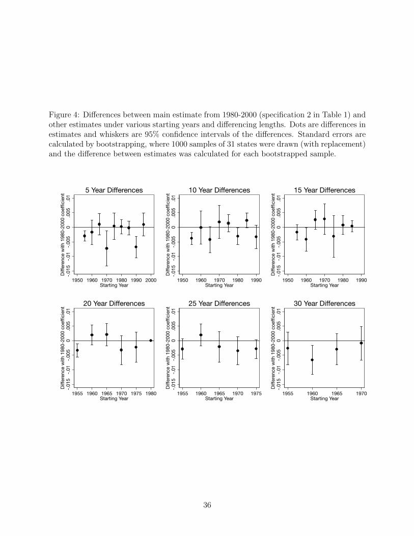
Figure 4: Differences between main estimate from 1980-2000 (specification 2 in Table 1) andother estimates under various starting years and differencing lengths. Dots are differences inestimates and whiskers are 95% confidence intervals of the differences. Standard errors arecalculated by bootstrapping, where 1000 samples of 31 states were drawn (with replacement)and the difference between estimates was calculated for each bootstrapped sample.

-.015

-.01

-.005

0.0

05.0

1Di

ffere

nce

with

198

0-20

00 c

oeffi

cien

t

1950 1960 1970 1980 1990 2000Starting Year

5 Year Differences

-.015

-.01

-.005

0.0

05.0

1Di

ffere

nce

with

198

0-20

00 c

oeffi

cien

t

1950 1960 1970 1980 1990Starting Year

10 Year Differences

-.015

-.01

-.005

0.0

05.0

1Di

ffere

nce

with

198

0-20

00 c

oeffi

cien

t1950 1960 1970 1980 1990

Starting Year

15 Year Differences

-.015

-.01

-.005

0.0

05.0

1Di

ffere

nce

with

198

0-20

00 c

oeffi

cien

t

1955 1960 1965 1970 1975 1980Starting Year

20 Year Differences

-.015

-.01

-.005

0.0

05.0

1Di

ffere

nce

with

198

0-20

00 c

oeffi

cien

t

1955 1960 1965 1970 1975Starting Year

25 Year Differences

-.015

-.01

-.005

0.0

05.0

1Di

ffere

nce

with

198

0-20

00 c

oeffi

cien

t

1955 1960 1965 1970Starting Year

30 Year Differences

36

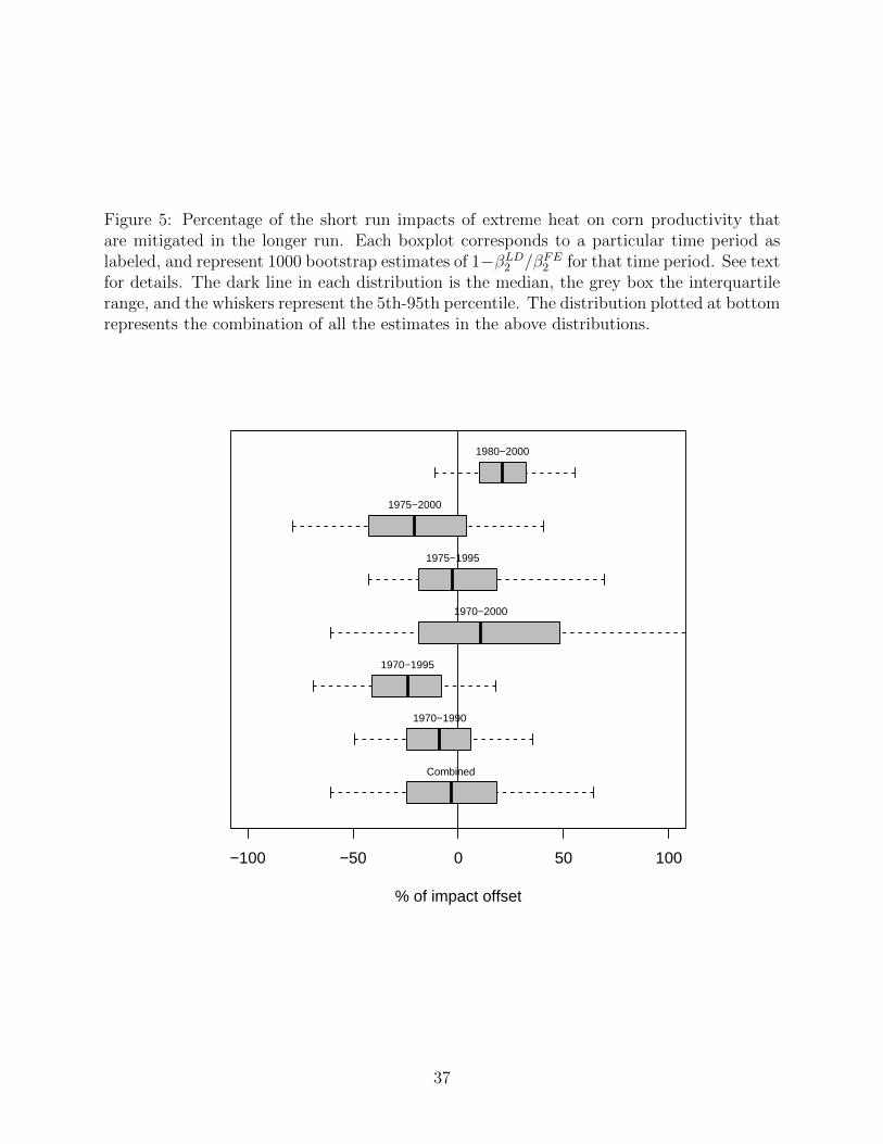
Figure 5: Percentage of the short run impacts of extreme heat on corn productivity thatare mitigated in the longer run. Each boxplot corresponds to a particular time period aslabeled, and represent 1000 bootstrap estimates of 1−βLD

2 /βFE2 for that time period. See text

for details. The dark line in each distribution is the median, the grey box the interquartilerange, and the whiskers represent the 5th-95th percentile. The distribution plotted at bottomrepresents the combination of all the estimates in the above distributions.

−100 −50 0 50 100

% of impact offset

1970−1990

1970−1995

1970−2000

1975−1995

1975−2000

1980−2000

Combined

37

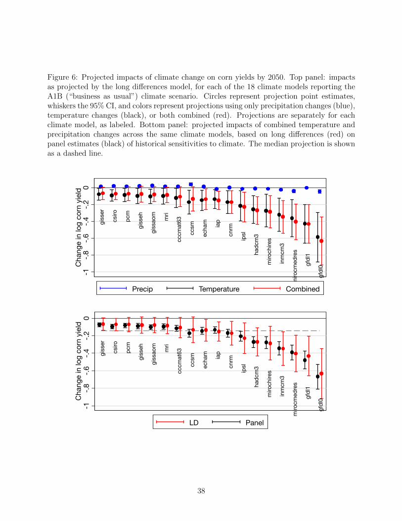
Figure 6: Projected impacts of climate change on corn yields by 2050. Top panel: impactsas projected by the long differences model, for each of the 18 climate models reporting theA1B (“business as usual”) climate scenario. Circles represent projection point estimates,whiskers the 95% CI, and colors represent projections using only precipitation changes (blue),temperature changes (black), or both combined (red). Projections are separately for eachclimate model, as labeled. Bottom panel: projected impacts of combined temperature andprecipitation changes across the same climate models, based on long differences (red) onpanel estimates (black) of historical sensitivities to climate. The median projection is shownas a dashed line.

giss

er

csiro

pcm

giss

eh

giss

aom

mri

cccm

at63

ccsm

echa

m iap

cnrm

ipsl

hadc

m3

miro

chire

s

inm

cm3

miro

cmed

res

gfdl

1

gfdl

0

-1-.8

-.6-.4

-.20

Cha

nge

in lo

g co

rn y

ield

Precip Temperature Combined

giss

er

csiro

pcm

giss

eh

giss

aom

mri

cccm

at63

ccsm

echa

m iap

cnrm

ipsl

hadc

m3

miro

chire

s

inm

cm3

miro

cmed

res

gfdl

1

gfdl

0

-1-.8

-.6-.4

-.20

Cha

nge

in lo

g co

rn y

ield

LD Panel

38

Tab

le1:

Com

par

ison

oflo

ng

diff

eren

ces

and

pan

eles

tim

ates

ofth

eim

pac

tsof

tem

per

ature

and

pre

cipit

atio

non

US

corn

yie

lds

(1)

(2)

(3)

(4)

(5)

(6)

(7)

(8)

Diff

sD

iffs

Pan

elP

an

elD

iffs

Diff

sP

an

elP

an

elG

DD

bel

owth

resh

old

-0.0

001

0.0002

0.0

004∗∗∗

0.0

002∗∗

-0.0

001

0.0

003∗

0.0

005∗∗∗

0.0

003∗∗∗

(0.0

003)

(0.0

002)

(0.0

001)

(0.0

001)

(0.0

003)

(0.0

002)

(0.0

001)

(0.0

001)

GD

Dab

ove

thre

shol

d-0

.005

3∗∗∗

-0.0

044∗∗∗

-0.0

056∗∗∗

-0.0

062∗∗∗

-0.0

043∗∗∗

-0.0

037∗∗∗

-0.0

048∗∗∗

-0.0

054∗∗∗

(0.0

010)

(0.0

008)

(0.0

006)

(0.0

007)

(0.0

009)

(0.0

009)

(0.0

005)

(0.0

006)

Pre

cip

bel

owth

resh

old

0.05

15∗∗

0.02

97∗∗

0.0

118∗∗∗

0.0

095∗

0.0

253∗∗

0.0

115∗∗

0.0

068∗∗∗

0.0

057∗∗∗

(0.0

194)

(0.0

125)

(0.0

027)

(0.0

048)

(0.0

123)

(0.0

046)

(0.0

015)

(0.0

019)

Pre

cip

abov

eth

resh

old

0.00

36∗∗

0.00

34∗∗∗

-0.0

008

0.0

001

0.0

024

0.0

029∗∗∗

-0.0

018∗∗

-0.0

008

(0.0

017)

(0.0

008)

(0.0

005)

(0.0

004)

(0.0

015)

(0.0

007)

(0.0

007)

(0.0

005)

Con

stan

t0.

2655∗∗∗

0.23

97∗∗∗

3.5

721∗∗∗

4.1

872∗∗∗

0.2

674∗∗∗

0.2

400∗∗∗

3.2

423∗∗∗

3.8

577∗∗∗

(0.0

319)

(0.0

124)

(0.2

491)

(0.3

013)

(0.0

307)

(0.0

115)

(0.2

647)

(0.3

349)

Ob

serv

atio

ns

1531

1531

48465

48465

1531

1531

48465

48465

Rsq

uar

ed0.

258

0.610

0.5

90

0.8

63

0.2

43

0.6

02

0.5

93

0.8

64

Fix

edE

ffec

tsN

one

Sta

teC

ty,

Yr

Cty

,S

tate

-Yr

Non

eS

tate

Cty

,Y

rC

ty,

Sta

te-Y

rT

thre

shol

d29

C29

C29C

29C

28C

28C

28C

28C

Pth

resh

old

42cm

42cm

42cm

42cm

50cm

50cm

50cm

50cm

Dat

aar

efo

rU

Sco

unti

esea

stof

the

100t

hm

erid

ian

,1980-2

000.

Sp

ecifi

cati

on

s1-2

an

d4-5

are

esti

mate

dw

ith

lon

gd

iffer

ence

san

d3

an

d6

wit

han

annu

alp

anel

;se

ete

xt

for

det

ails

.S

pec

ifica

tion

s1-3

use

pie

cew

ise

lin

ear

thre

shold

sas

chose

nby

the

lon

gd

iffer

ence

sm

od

el,

an

d4-6

use

thre

shold

sas

chos

enby

the

pan

elm

od

el.

Reg

ress

ion

sar

ew

eighte

dby

1980

cou

nty

corn

are

a(l

on

gd

iffer

ence

s)or

by

1980-2

000

aver

age

corn

are

a(p

an

el).

Sta

nd

ard

erro

rsar

ecl

ust

ered

atth

est

ate

leve

l.A

ster

isks

ind

icate

stati

stic

al

sign

ifica

nce

at

the

1%∗∗∗ ,

5%∗∗

,an

d10%∗

leve

ls.

39

Table 2: The effect of climate on yields estimated with a panel of differences.(1) (2) (3) (4)

1955-1995 1955-1995 1960-2000 1960-2000GDD below threshold 0.0008∗∗∗ 0.0007∗ 0.0004∗∗∗ 0.0003∗

(0.0003) (0.0004) (0.0001) (0.0002)

GDD above threshold -0.0066∗∗∗ -0.0058∗∗∗ -0.0031∗∗∗ -0.0023∗∗

(0.0013) (0.0020) (0.0007) (0.0010)

Precip below threshold 0.0356∗∗∗ 0.0376∗∗∗ 0.0203 0.0166(0.0079) (0.0093) (0.0135) (0.0115)

Precip above threshold 0.0017 0.0033∗ 0.0008 0.0014(0.0015) (0.0017) (0.0015) (0.0020)

Observations 2060 2060 2604 2604R squared 0.621 0.565 0.688 0.699Fixed Effects State Yr Cty Yr State Yr Cty YrT threshold 29 29 29 29P threshold 42 42 42 42

Dependent variable in all regressions is the difference in the log of smoothed corn yields. Data are a twoperiod panel with 20 year differences. Periods are 1955-1975 and 1975-1995 in Columns 1-2. Periods are1960-1980 and 1980-2000 in Columns 3-4. The sample of counties is limited to the 1980-2000 corn samplefrom Table 1. Regressions in Columns 1-2 are weighted by 1955 smoothed corn acres. Regressions inColumns 3-4 are weighted by 1960 smoothed corn acres. Standard errors are clustered at the state level.Asterisks indicate statistical significance at the 1% ∗∗∗,5% ∗∗, and 10% ∗ levels.

40

Table 3: Effects of climate variation on crop revenuesCorn Main Spring Crops

(1) (2) (3) (4)Panel Diffs Panel Diffs

GDD below threshold 0.0005∗∗∗ 0.0003 0.0002 0.0003(0.0001) (0.0002) (0.0001) (0.0003)

GDD above threshold -0.0046∗∗∗ -0.0042∗∗∗ -0.0024∗∗∗ -0.0023∗∗

(0.0005) (0.0009) (0.0003) (0.0011)

Precip below threshold 0.0068∗∗∗ 0.0107∗∗ 0.0058∗∗∗ 0.0116∗

(0.0016) (0.0048) (0.0014) (0.0058)

Precip above threshold -0.0014∗∗ 0.0035∗∗∗ -0.0012∗∗ 0.0016(0.0007) (0.0010) (0.0005) (0.0016)

Constant 3.9556∗∗∗ -0.0116 4.7926∗∗∗ 0.0121(0.2539) (0.0122) (0.3619) (0.0210)

Observations 48465 1516 48465 1531Mean of Dep Variable 5.55 -0.01 5.36 0.03R squared 0.568 0.579 0.490 0.454Fixed Effects Cty, Yr State Cty, Yr State

In Columns 1 and 2 the dependent variable is log of agricultural revenue per acre from corn. Dependentvariable in Columns 3 and 4 is log of agricultural revenue per acre from 6 main crops grown during thespring season (corn, soy, cotton, spring wheat, hay, and rice). Revenues calculated as yield per acremultiplied by state-level annual prices. Panel regressions are weighted by average area cultivated to corn(Column 1) and main crops (Column 3) from 1978-2002. Long differences regressions are weighted bysmoothed corn area in 1980 (Column 2) and smoothed area cultivated to main crops (Column 4).Temperature threshold is 28 and precipitation threshold is 50 in all regressions. Standard errors areclustered at the state level. Asterisks indicate statistical significance at the 1% ∗∗∗,5% ∗∗, and 10% ∗ levels.

41

Table 4: Effects of climate variation on alternate adjustment margins(1) (2) (3) (4) (5)

Corn area Corn share Farm area Num. farms PopulationGDD below threshold 0.0010 0.0003∗∗∗ -0.0001 -0.0002 0.0006∗∗

(0.0012) (0.0001) (0.0001) (0.0002) (0.0003)

GDD above threshold -0.0005 -0.0009∗∗ 0.0000 -0.0007 -0.0008(0.0038) (0.0004) (0.0004) (0.0010) (0.0015)

Precip below threshold 0.0264 -0.0004 0.0037 0.0021 -0.0236∗∗

(0.0637) (0.0034) (0.0035) (0.0029) (0.0106)

Precip above threshold -0.0051 -0.0016 0.0007 -0.0013 0.0047∗

(0.0063) (0.0010) (0.0007) (0.0033) (0.0024)

Constant -0.0130 -0.0174∗∗∗ -0.0614∗∗∗ -0.1836∗∗∗ 0.0144(0.0687) (0.0045) (0.0075) (0.0157) (0.0160)

Observations 1511 1516 1523 1526 1526Mean of Dep Variable 0.075 0.002 -0.068 -0.202 0.045R squared 0.645 0.418 0.399 0.488 0.392Fixed Effects State State State State StateT threshold 29 29 29 29 29P threshold 42 42 42 42 42

Dependent variable is difference in log of corn acres (Column 1), difference in share of agricultural areaplanted to corn (Column 2), difference in total log farm area (Column 3), difference in log number of farms(Column 4), and difference in log county population (Column 5). All regressions are long differences from1980-2000, with the sample trimmed of extreme outliers in the temperature data. All regressions areweighted by average agricultural area from 1978-2002. Standard errors are clustered at the state level.Asterisks indicate statistical significance at the 1% ∗∗∗,5% ∗∗, and 10% ∗ levels.

42

Tab

le5:

Het

erog

enou

seff

ects

ofcl

imat

eva

riat

ion

onco

rnyie

lds

(1)

(2)

(3)

(4)

(5)

(6)

GD

Dab

ove

-0.0

0427∗∗∗

-0.0

0568∗∗∗

-0.0

0427∗∗∗

-0.0

0424∗∗∗

-0.0

0395∗∗∗

-0.0

0413∗∗∗

(0.0

0115)

(0.0

0099)

(0.0

0104)

(0.0

0095)

(0.0

0082)

(0.0

0085)

GD

Dab

ove*

SD

GD

Dab

ove,

1950

-198

0-0

.00002

(0.0

0005)

GD

Dab

ove*

GD

Dab

ove,

1960

-198

00.0

0001

(0.0

0003)

GD

Dab

ove*

GD

Dab

ove,

1970

-198

0-0

.00000

(0.0

0004)

GD

Dab

ove*

Sta

teG

DD

abov

e,19

60-1

980

-0.0

0005

(0.0

0006)

GD

Dab

ove*

Rep

ub

lica

nvo

tesh

are,

2000

0.0

0197

(0.0

0424)

GD

Dab

ove*

Hig

hsc

hool

grad

.ra

te,

1980

-0.0

0002

(0.0

0005)

Ob

serv

atio

ns

1531

1531

1531

1531

1530

1531

Mea

nof

Dep

Var

iable

0.2

40.2

40.2

40.2

40.2

40.2

4R

squ

ared

0.6

10

0.6

15

0.6

10

0.6

10

0.6

23

0.6

14

Fix

edE

ffec

tsS

tate

Sta

teS

tate

Sta

teS

tate

Sta

te

Dep

end

ent

vari

able

isth

ed

iffer

ence

(198

0-20

00)

inth

elo

gof

smooth

edco

rnyie

lds.

Th

esa

mp

leof

cou

nti

esis

lim

ited

toth

e1980-2

000

corn

sam

ple

from

Tab

le1,

and

regr

essi

ons

are

wei

ghte

dby

1980

corn

acr

es.

All

vari

ab

les

inth

eta

ble

oth

erth

an

GD

Dabo

veth

resh

old

are

dem

ean

ed.

On

lyco

effici

ents

onG

DD

abov

eth

resh

old

and

rele

vant

inte

ract

ion

sare

rep

ort

ed,

bu

tall

leve

leff

ects

,G

DD

bel

owth

resh

old

,P

reci

pit

ati

on

ab

ove

thre

shol

d,

and

Pre

cip

itat

ion

bel

owth

resh

old

are

als

oin

clu

ded

inth

ere

gre

ssio

n.

Tem

per

atu

reth

resh

old

is29C

an

dp

reci

pit

ati

on

thre

shold

is42cm

inal

lsp

ecifi

cati

ons.

Sta

nd

ard

erro

rsar

ecl

ust

ered

at

the

state

leve

l.A

ster

isks

ind

icate

stati

stic

al

sign

ifica

nce

at

the

1%∗∗∗ ,

5%∗∗

,an

d10%∗

leve

ls.

43

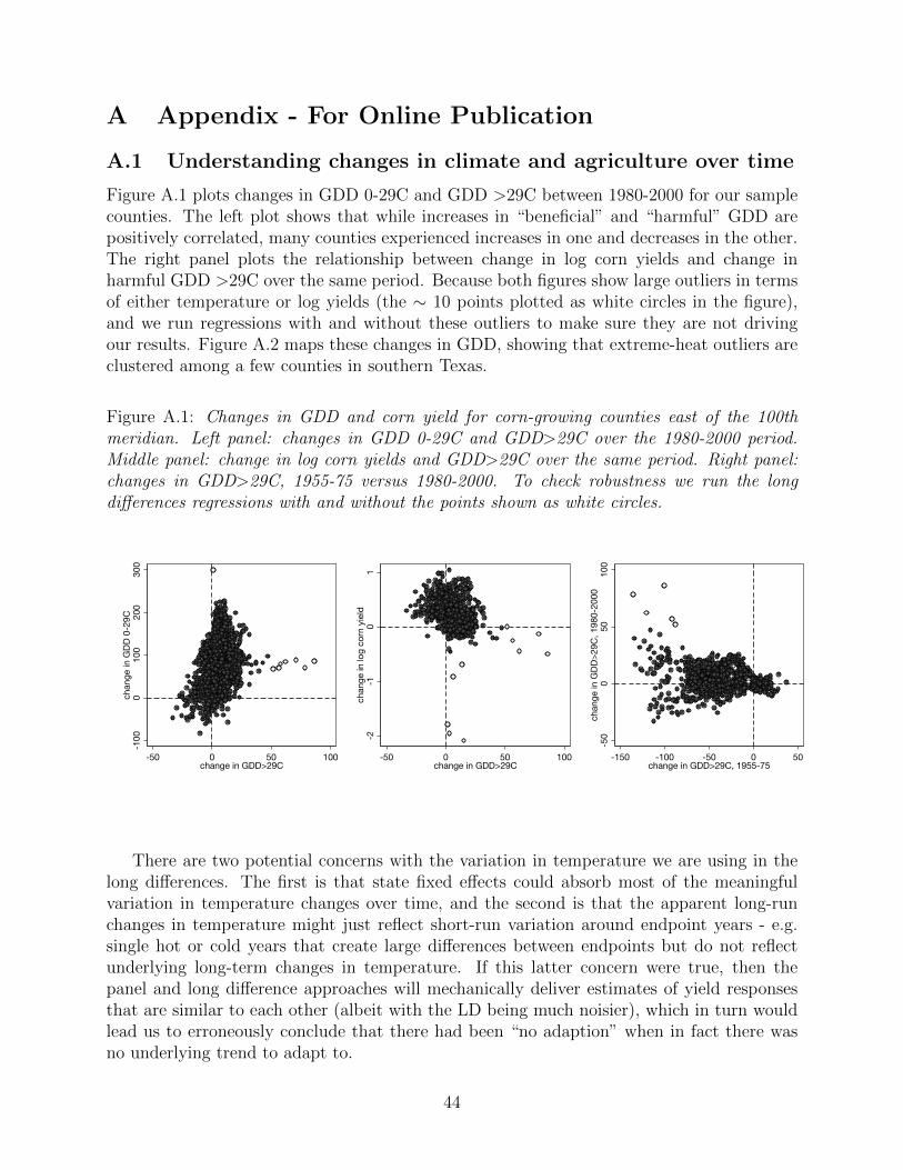
A Appendix - For Online Publication

A.1 Understanding changes in climate and agriculture over time

Figure A.1 plots changes in GDD 0-29C and GDD >29C between 1980-2000 for our samplecounties. The left plot shows that while increases in “beneficial” and “harmful” GDD arepositively correlated, many counties experienced increases in one and decreases in the other.The right panel plots the relationship between change in log corn yields and change inharmful GDD >29C over the same period. Because both figures show large outliers in termsof either temperature or log yields (the ∼ 10 points plotted as white circles in the figure),and we run regressions with and without these outliers to make sure they are not drivingour results. Figure A.2 maps these changes in GDD, showing that extreme-heat outliers areclustered among a few counties in southern Texas.

Figure A.1: Changes in GDD and corn yield for corn-growing counties east of the 100thmeridian. Left panel: changes in GDD 0-29C and GDD>29C over the 1980-2000 period.Middle panel: change in log corn yields and GDD>29C over the same period. Right panel:changes in GDD>29C, 1955-75 versus 1980-2000. To check robustness we run the longdifferences regressions with and without the points shown as white circles.

-100

010

020

030

0ch

ange

in G

DD 0

-29C

-50 0 50 100change in GDD>29C

-2-1

01

chan

ge in

log

corn

yie

ld

-50 0 50 100change in GDD>29C

-50

050

100

chan

ge in

GDD

>29C

, 198

0-20

00

-150 -100 -50 0 50change in GDD>29C, 1955-75

There are two potential concerns with the variation in temperature we are using in thelong differences. The first is that state fixed effects could absorb most of the meaningfulvariation in temperature changes over time, and the second is that the apparent long-runchanges in temperature might just reflect short-run variation around endpoint years - e.g.single hot or cold years that create large differences between endpoints but do not reflectunderlying long-term changes in temperature. If this latter concern were true, then thepanel and long difference approaches will mechanically deliver estimates of yield responsesthat are similar to each other (albeit with the LD being much noisier), which in turn wouldlead us to erroneously conclude that there had been “no adaption” when in fact there wasno underlying trend to adapt to.

44

Figure A.2: Map of changes in GDD 0-29C and GDD above 29C between 1980-2000, forcorn-growing counties east of the 100th meridian. Rightmost panel re-plots the change inGDD >29 dropping the outliers indicated in Figure A.1.

GDD 0−29C

●

●

●

●

●

●●

●

●

●

●

●●

●●

●

●

●

●

●●

●

●

●

●

●

●

●●●

●

●●

●●

●

●●

●●

●

●

● ●

●

●

● ●

●●

●

●

●●

●

●

●

●●

●●●

●●

●●

●●

●

●● ●

●●

●

●●

●●

●●

●●●●●

● ●●

●●

●

●●

●

●●●

●●

●

●

●

●

●

●●●

●●

● ●

●

●

●●

●

●

●

●●●

●

●

●●●

●

●●●

●●

●

●●

●

●●

●●●

●●●●●●●●

●●

●

●●● ●

●

●

●

●

●

●

●

●

●

●●●

●

●

●

●

●●

●

●

●

●●

●

●

●●

●

●

●

●

●

● ●

●

●

●

●

●●

●

●●

●

●●

●●

●

●

●

●●

●● ●

●

●●●

●●●●

●

●●●

●●

●●

●●

●●

●●

●●

●

●

●

●

●●

● ● ●

●

●

●

●

●●

●

●

●●●

●●

●

●

●●●

●

●●

●

●

●●

●

●

● ● ●●

●

●

●

●

●

●●●●

●●

●

●

● ●

●

●

●●

●

●●●●●

●

●● ●

●

●

●

●

●

●

●

●

●●

●●

●

●

●

●

●

●●●●

●

●

●

●

●

●

●

●●

●●

●●

●

●

●

●●●

●

●●

●●

●●

●●●

●

●

●

●

●

●

●

●●

●● ●

●●

●

●

●

●

●

●

●

●

●

●

●

●

● ●● ●

●●

●

●

●●

●

●●

●

●

●●●

●

●

●

●

●

●

●

●

●

●●

●

●

●●

●

●

●

●●

●●

●

●

●

●

●●●

●

●●

●● ●

●●

●

●

●

●

●● ●

●

●

●

●●

●●

●

●●

●

●●

●●● ●

●

●

●

●

●

●

●

● ●●

● ●

●

●

● ●●

●

● ●●

●

●●

●

●

●

●●

●●

●

●

●

●

●

●

●●

●

●

●

●

●●

●

● ●●

●

●

●●

●●●

●

●●●●

●

●●

●

●

●

●

●●

●●

●●

●●

●●

●

●

●

●●

●●

●

●

●

●

●●

● ●

● ●●

●

●●

●●

●●

●

●●●●●

●

●

●●

●●

●●● ●●●●

●

●● ●

●

● ●

●●●

●●

●

●

●

●

●●●●

●

●●

●●●

●●

●

●●

●●

●●

●●●

●

●

●

●

●●

●

● ●●●

●

●

●

●●●

●●

●

●● ●

●●

●

●

●●●

●

● ●

●● ●●● ●●

●

● ●

●

●●

●●

●

●

●●

●

●●

● ●●

●●

●

● ● ●

●

●

●

●●

● ●

●

●●

●

●●

●●

●●●

●

●●●

●●●●●●

●

●●

●

●

●

●

●

●

●● ●

●

●●

●●

●

●

●●●

● ●

●

●●

●●

● ●●

●●

●

●●

●

● ●

●

●

●● ●

●

●

●●●●

●

●

●

●●

●●

●●

●●

●

●●

●●

●●●

●

●

●

●

●●●

●● ●

●

●

●●

●

●● ●

● ●

●

●●

●

●●

●

●● ●●● ●● ● ●●

●

●●

● ●●●●

●●●

●●

●

●●

●

●

●●

●

●

●●

●

●●

●

●●

●●

●

●●

●

●●

●

●●

●●

●●

●●

●●●

●

●

●

●

●

●●

●

●

●●

●●

●●

●

●●●

●

●

●

●●

●

●

●

●

●●

●●

●

●

●●●

●●●

●●

●

●

●

●

● ●

●

●

●

●

●

●

●

●

● ●●●●●

●●

●

●

●●

●

●●●

●●● ●

● ●

●● ●● ●●● ●● ●

●●

●●

●●

●

●●●●

●●

●

●

●

●

●●

●

●

●

●

●

● ●●●

●●

●

●

●

●

●●

●

●

●

●

●

●

●

●

●

●

●●

●

●

●

●●

●

●

●

●

●

●

●●

●●

●

●

●

●●

●

●●

●

●

●

●●

●

●●

●

●●

●

●

●

●

●●

●

●

●

●●

● ●●

●

●

●

●

●

●●

●●

●

●

●

●●

●●

●

●

●●

●

● ●●●

●

●

●

●

●

●

●

●●

●●

●

●

●

●●●●

●

●

●

●●●

●● ●●

●

●

●

●

●

●

●

●●

●

●● ●●

●

●

●●

●

●

●

●●●●

●

●

●

●

●

●

●

●●

●

●

●

●

●

● ●●

●●

● ●

●●

● ●

●

●●●●

●

●●

●

●●●

●

●

●● ●●

●

●

●

●

●

●

●●

●

●

●

●

●

●●

●●

●●

●

●●●

●●

●

●●●

●●

●

●●● ●●● ●

●

●

●

●

●

●

●

●

●

●●●

●

●●● ●

●

●●

●

●●

●●

●

●

●

●

●

●

●

●●

●●

●● ●

●●

●●

●

●●

●

●

●●

●●

●

●

●●

●

●

●●

●

●

●

●

●

●●●

●

●

●●

●●

●

●

●

●●

●

●●

●

●

●

●●

●

●

●

●●

● ●

●

●●●

●●

●● ●●

●●

●●

●●

●

●●

●

●●

●

●●

●●

●

●

●

●● ●

●●

●

●● ●

●

●

●●●

●

●

●

●●●

●● ●

●

●

●●●

●

●

●

● ●●

● ●

●

● ●●●

●●●●

●

●●●

●

●

●●●

●●

●

●

●● ●

●

●

●

●

●●

●

●●

●●●●

●

●●●●●

●

●●●●●

●●

●●●

●● ●●

●● ●

●

●

●●

●●

●

●●

●●●

●●●

● ●● ●● ●●●

●

● ●●

●

●

●

●●●●●

●

●

●●● ●

●●●

●

● ●

●●●

●

●●

●●

●●

● ●●

●●

●

●● ●

●

●

● ●

●

●●

●●●

●

● ●● ●●

●●●

● ●

●●●

●

●●● ●

●● ●●●● ●

●●

●●●

●

●

●

●

●

●

●

●●●●

●●

●

●●●

●●●

●●

●●●

●

●●

●●

●

●●

●●●

●

●

●

●

●

●●●

●●

●●●

●

●● ●

●●

●

●

●●

●

●

●●

●

● ●

●

●

●●

●●

●●●

●●

●●

●●

●

●

●

●

●●●

●

●

●

●●

●

●●

●

●

● ●

●●

●

●●

●

●

●●

●●

●

●●

●

●

●● ●● ●

●●●

●●

●●●

●

●

● ●

●

●

●

●●

●●●

●●●

●● ●

●● ●

●

●

●

●

●●

●

●●

●

●

●

●●●

●

●

●●●

●● ●

●●

●

●●

●

●●●

● ●

●

●

● ●●●●

●

●

●

●

●

●

●

●

●●

●

●● ●

● ●●●

●●●

●

●●

● ●

●●

●●●

●

●●

●●

●●●

●●

●

●●

●

●●●

●

● ● ● ●●

●●●

●●

●

●

●●●●●

●●

●

●

●● ●●●

●●

●●

●● ●●

●●

●●

●●●

●●●

●●●

●

●

●

●

●

●●●●●

●●●

●

●●

●●

●●

●● ●

●●

●●

●●

●●●

●●

●

●

●

●●● ●●● ●

●●●

●

●

●●

●

●●

●

●

●●

●

●

●

●●

●

●

●

●

●

●●

●

●● ●

●

●●

●●

●● ●

●●

● ●

● ●

●●●

●●

●

●

● ●●●

●●

●● ●●

●●● ●●

●

●●●

●● ●●●

●●●

●

●

●

●●

●●●

●

●

●

●●

●

● ●●

●●● ● ●

●●

●●

●● ●●●●

●

●●

●● ●●

●

●●● ●

●

●

●

●●●

●●

●

●●

●

●● ●●

●

● ●●●●

●

●

●●●●

●●

●

●

●

●●●

●

●

●

●●

●

●

●

●

●

●

●●

●

●

●

●

●●

●

●

●

●

●

●●

●●

●

●

●●●

●●

●

● ●●

●

●

●

●

●

●

●

●●

●

●●

●

●

●

●

●

●

●●

●●

●

●

●

●●

●

●

●●

●

●

●

●●

●●

●

●

●

●

●●

●

● ●

●

●

●

●

●

●

●

●

●●

●

●

●

●

●

●●

● ●●

●

●

●

●●

●

●

●

●●

●

●

●

●

●

●

●

●

● ●●●

●

●

●

●

●●●

●

● ●●

● ●

●●●

●

●

●

●

●●●

●

●

●●

●

●

●

●●

●

●

●

●

●

●● ●●●●●●

●●

●●

●●●●●●

●●●●

●●

● ●●

●

●●

●●

●

●

●

●● ●

●

●●

●

●

●

●

● ●●

●

●

●●

●●

●

●

●●●

●●●

●

●

●

●

●

●●

●●

● ● ●●

●

●●

● ●●● ●

●

●

●●

●●

●

●●

●

● ●

●●

●●●

●

●

●

● ● ●●●

● ●

●●

● ●●

●

●

●

●

●

●●●●●●

●

●●

●●

●● ●

●●

●

●●●●

●

● ●

●

●

●

●●●

●

●●

●●●

●●

●

●

●●

●

●

●

●

●●

●

●

●●

●●

●

●

●●●

●●

●

●●●

●

●

●●

●

●●

●

●

●●

●● ●●

●

●

●●

●

●

●

● ●

●●

●

●

●

●

●

●●

●

●●

●●

●

●

●

●

●

●●

●

●

●●●

●

●

●●

●

●●

●

●

●

●

●

●●

●

●

●

●●

●●●

●

change in GDD 0−29C

−100 0 100 200 300

GDD >29C

●

●

●

●

●

●●

●

●

●

●

●●

●●

●

●

●

●

●●

●

●

●

●

●

●

●●●

●

●●

●●

●

●●

●●

●

●

● ●

●

●

● ●

●●

●

●

●●

●

●

●

●●

●●●

●●

●●

●●

●

●● ●

●●

●

●●

●●

●●

●●●●●

● ●●

●●

●

●●

●

●●●

●●

●

●

●

●

●

●●●

●●

● ●

●

●

●●

●

●

●

●●●

●

●

●●●

●

●●●

●●

●

●●

●

●●

●●●

●●●●●●●●

●●

●

●●● ●

●

●

●

●

●

●

●

●

●

●●●

●

●

●

●

●●

●

●

●

●●

●

●

●●

●

●

●

●

●

● ●

●

●

●

●

●●

●

●●

●

●●

●●

●

●

●

●●

●● ●

●

●●●

●●●●

●

●●●

●●

●●

●●

●●

●●

●●

●

●

●

●

●●

● ● ●

●

●

●

●

●●

●

●

●●●

●●

●

●

●●●

●

●●

●

●

●●

●

●

● ● ●●

●

●

●

●

●

●●●●

●●

●

●

● ●

●

●

●●

●

●●●●●

●

●● ●

●

●

●

●

●

●

●

●

●●

●●

●

●

●

●

●

●●●●

●

●

●

●

●

●

●

●●

●●

●●

●

●

●

●●●

●

●●

●●

●●

●●●

●

●

●

●

●

●

●

●●

●● ●

●●

●

●

●

●

●

●

●

●

●

●

●

●

● ●● ●

●●

●

●

●●

●

●●

●

●

●●●

●

●

●

●

●

●

●

●

●

●●

●

●

●●

●

●

●

●●

●●

●

●

●

●

●●●

●

●●

●● ●

●●

●

●

●

●

●● ●

●

●

●

●●

●●

●

●●

●

●●

●●● ●

●

●

●

●

●

●

●

● ●●

● ●

●

●

● ●●

●

● ●●

●

●●

●

●

●

●●

●●

●

●

●

●

●

●

●●

●

●

●

●

●●

●

● ●●

●

●

●●

●●●

●

●●●●

●

●●

●

●

●

●

●●

●●

●●

●●

●●

●

●

●

●●

●●

●

●

●

●

●●

● ●

● ●●

●

●●

●●

●●

●

●●●●●

●

●

●●

●●

●●● ●●●●

●

●● ●

●

● ●

●●●

●●

●

●

●

●

●●●●

●

●●

●●●

●●

●

●●

●●

●●

●●●

●

●

●

●

●●

●

● ●●●

●

●

●

●●●

●●

●

●● ●

●●

●

●

●●●

●

● ●

●● ●●● ●●

●

● ●

●

●●

●●

●

●

●●

●

●●

● ●●

●●

●

● ● ●

●

●

●

●●

● ●

●

●●

●

●●

●●

●●●

●

●●●

●●●●●●

●

●●

●

●

●

●

●

●

●● ●

●

●●

●●

●

●

●●●

● ●

●

●●

●●

● ●●

●●

●

●●

●

● ●

●

●

●● ●

●

●

●●●●

●

●

●

●●

●●

●●

●●

●

●●

●●

●●●

●

●

●

●

●●●

●● ●

●

●

●●

●

●● ●

● ●

●

●●

●

●●

●

●● ●●● ●● ● ●●

●

●●

● ●●●●

●●●

●●

●

●●

●

●

●●

●

●

●●

●

●●

●

●●

●●

●

●●

●

●●

●

●●

●●

●●

●●

●●●

●

●

●

●

●

●●

●

●

●●

●●

●●

●

●●●

●

●

●

●●

●

●

●

●

●●

●●

●

●

●●●

●●●

●●

●

●

●

●

● ●

●

●

●

●

●

●

●

●

● ●●●●●

●●

●

●

●●

●

●●●

●●● ●

● ●

●● ●● ●●● ●● ●

●●

●●

●●

●

●●●●

●●

●

●

●

●

●●

●

●

●

●

●

● ●●●

●●

●

●

●

●

●●

●

●

●

●

●

●

●

●

●

●

●●

●

●

●

●●

●

●

●

●

●

●

●●

●●

●

●

●

●●

●

●●

●

●

●

●●

●

●●

●

●●

●

●

●

●

●●

●

●

●

●●

● ●●

●

●

●

●

●

●●

●●

●

●

●

●●

●●

●

●

●●

●

● ●●●

●

●

●

●

●

●

●

●●

●●

●

●

●

●●●●

●

●

●

●●●

●● ●●

●

●

●

●

●

●

●

●●

●

●● ●●

●

●

●●

●

●

●

●●●●

●

●

●

●

●

●

●

●●

●

●

●

●

●

● ●●

●●

● ●

●●

● ●

●

●●●●

●

●●

●

●●●

●

●

●● ●●

●

●

●

●

●

●

●●

●

●

●

●

●

●●

●●

●●

●

●●●

●●

●

●●●

●●

●

●●● ●●● ●

●

●

●

●

●

●

●

●

●

●●●

●

●●● ●

●

●●

●

●●

●●

●

●

●

●

●

●

●

●●

●●

●● ●

●●

●●

●

●●

●

●

●●

●●

●

●

●●

●

●

●●

●

●

●

●

●

●●●

●

●

●●

●●

●

●

●

●●

●

●●

●

●

●

●●

●

●

●

●●

● ●

●

●●●

●●

●● ●●

●●

●●

●●

●

●●

●

●●

●

●●

●●

●

●

●

●● ●

●●

●

●● ●

●

●

●●●

●

●

●

●●●

●● ●

●

●

●●●

●

●

●

● ●●

● ●

●

● ●●●

●●●●

●

●●●

●

●

●●●

●●

●

●

●● ●

●

●

●

●

●●

●

●●

●●●●

●

●●●●●

●

●●●●●

●●

●●●

●● ●●

●● ●

●

●

●●

●●

●

●●

●●●

●●●

● ●● ●● ●●●

●

● ●●

●

●

●

●●●●●

●

●

●●● ●

●●●

●

● ●

●●●

●

●●

●●

●●

● ●●

●●

●

●● ●

●

●

● ●

●

●●

●●●

●

● ●● ●●

●●●

● ●

●●●

●

●●● ●

●● ●●●● ●

●●

●●●

●

●

●

●

●

●

●

●●●●

●●

●

●●●

●●●

●●

●●●

●

●●

●●

●

●●

●●●

●

●

●

●

●

●●●

●●

●●●

●

●● ●

●●

●

●

●●

●

●

●●

●

● ●

●

●

●●

●●

●●●

●●

●●

●●

●

●

●

●

●●●

●

●

●

●●

●

●●

●

●

● ●

●●

●

●●

●

●

●●

●●

●

●●

●

●

●● ●● ●

●●●

●●

●●●

●

●

● ●

●

●

●

●●

●●●

●●●

●● ●

●● ●

●

●

●

●

●●

●

●●

●

●

●

●●●

●

●

●●●

●● ●

●●

●

●●

●

●●●

● ●

●

●

● ●●●●

●

●

●

●

●

●

●

●

●●

●

●● ●

● ●●●

●●●

●

●●

● ●

●●

●●●

●

●●

●●

●●●

●●

●

●●

●

●●●

●

● ● ● ●●

●●●

●●

●

●

●●●●●

●●

●

●

●● ●●●

●●

●●

●● ●●

●●

●●

●●●

●●●

●●●

●

●

●

●

●

●●●●●

●●●

●

●●

●●

●●

●● ●

●●

●●

●●

●●●

●●

●

●

●

●●● ●●● ●

●●●

●

●

●●

●

●●

●

●

●●

●

●

●

●●

●

●

●

●

●

●●

●

●● ●

●

●●

●●

●● ●

●●

● ●

● ●

●●●

●●

●

●

● ●●●

●●

●● ●●

●●● ●●

●

●●●

●● ●●●

●●●

●

●

●

●●

●●●

●

●

●

●●

●

● ●●

●●● ● ●

●●

●●

●● ●●●●

●

●●

●● ●●

●

●●● ●

●

●

●

●●●

●●

●

●●

●

●● ●●

●

● ●●●●

●

●

●●●●

●●

●

●

●

●●●

●

●

●

●●

●

●

●

●

●

●

●●

●

●

●

●

●●

●

●

●

●

●

●●

●●

●

●

●●●

●●

●

● ●●

●

●

●

●

●

●

●

●●

●

●●

●

●

●

●

●

●

●●

●●

●

●

●

●●

●

●

●●

●

●

●

●●

●●

●

●

●

●

●●

●

● ●

●

●

●

●

●

●

●

●

●●

●

●

●

●

●

●●

● ●●

●

●

●

●●

●

●

●

●●

●

●

●

●

●

●

●

●

● ●●●

●

●

●

●

●●●

●

● ●●

● ●

●●●

●

●

●

●

●●●

●

●

●●

●

●

●

●●

●

●

●

●

●

●● ●●●●●●

●●

●●

●●●●●●

●●●●

●●

● ●●

●

●●

●●

●

●

●

●● ●

●

●●

●

●

●

●

● ●●

●

●

●●

●●

●

●

●●●

●●●

●

●

●

●

●

●●

●●

● ● ●●

●

●●

● ●●● ●

●

●

●●

●●

●

●●

●

● ●

●●

●●●

●

●

●

● ● ●●●

● ●

●●

● ●●

●

●

●

●

●

●●●●●●

●

●●

●●

●● ●

●●

●

●●●●

●

● ●

●

●

●

●●●

●

●●

●●●

●●

●

●

●●

●

●

●

●

●●

●

●

●●

●●

●

●

●●●

●●

●

●●●

●

●

●●

●

●●

●

●

●●

●● ●●

●

●

●●

●

●

●

● ●

●●

●

●

●

●

●

●●

●

●●

●●

●

●

●

●

●

●●

●

●

●●●

●

●

●●

●

●●

●

●

●

●

●

●●

●

●

●

●●

●●●

●

change in GDD >29C

−50 0 50 100

GDD >29C (trimmed)

●

●

●

●

●

●●

●

●

●

●

●●

●●

●

●

●

●

●●

●

●

●

●

●

●

●●●

●

●●

●●

●

●●

●●

●

●

● ●

●

●

● ●

●●

●

●

●●

●

●

●

●●

●●●

●●

●●

●●

●

●● ●

●●

●

●●

●●

●●

●●●●●

● ●●

●●

●

●●

●

●●●

●●

●

●

●

●

●

●●●

●●

● ●

●

●

●●

●

●

●

●●●

●

●

●●●

●

●●●

●●

●

●●

●

●●

●●●

●●●●●●●●

●●

●

●●● ●

●

●

●

●

●

●

●

●

●

●●●

●

●

●

●

●●

●

●

●

●●

●

●

●●

●

●

●

●

●

● ●

●

●

●

●

●●

●

●●

●

●●

●●

●

●

●

●●

●● ●

●

●●●

●●●●

●

●●●

●●

●●

●●

●●

●●

●●

●

●

●

●

●●

● ● ●

●

●

●

●

●●

●

●

●●●

●●

●

●

●●●

●

●●

●

●

●●

●

●

● ● ●●

●

●

●

●

●

●●●●

●●

●

●

● ●

●

●

●●

●

●●●●●

●

●● ●

●

●

●

●

●

●

●

●

●●

●●

●

●

●

●

●

●●●●

●

●

●

●

●

●

●

●●

●●

●●

●

●

●

●●●

●

●●

●●

●●

●●●

●

●

●

●

●

●

●

●●

●● ●

●●

●

●

●

●

●

●

●

●

●

●

●

●

● ●● ●

●●

●

●

●●

●

●●

●

●

●●●

●

●

●

●

●

●

●

●

●

●●

●

●

●●

●

●

●

●●

●●

●

●

●

●

●●●

●

●●

●● ●

●●

●

●

●

●

●● ●

●

●

●

●●

●●

●

●●

●

●●

●●● ●

●

●

●

●

●

●

●

● ●●

● ●

●

●

● ●●

●

● ●●

●

●●

●

●

●

●●

●●

●

●

●

●

●

●

●●

●

●

●

●

●●

●

● ●●

●

●

●●

●●●

●

●●●●

●

●●

●

●

●

●

●●

●●

●●

●●

●●

●

●

●

●●

●●

●

●

●

●

●●

● ●

● ●●

●

●●

●●

●●

●

●●●●●

●

●

●●

●●

●●● ●●●●

●

●● ●

●

● ●

●●●

●●

●

●

●

●

●●●●

●

●●

●●●

●●

●

●●

●●

●●

●●●

●

●

●

●

●●

●

● ●●●

●

●

●

●●●

●●

●

●● ●

●●

●

●

●●●

●

● ●

●● ●●● ●●

●

● ●

●

●●

●●

●

●

●●

●

●●

● ●●

●●

●

● ● ●

●

●

●

●●

● ●

●

●●

●

●●

●●

●●●

●

●●●

●●●●●●

●

●●

●

●

●

●

●

●

●● ●

●

●●

●●

●

●

●●●

● ●

●

●●

●●

● ●●

●●

●

●●

●

● ●

●

●

●● ●

●

●

●●●●

●

●

●

●●

●●

●●

●●

●

●●

●●

●●●

●

●

●

●

●●●

●● ●

●

●

●●

●

●● ●

● ●

●

●●

●

●●

●

●● ●●● ●● ● ●●

●

●●

● ●●●●

●●●

●●

●

●●

●

●

●●

●

●

●●

●

●●

●

●●

●●

●

●●

●

●●

●

●●

●●

●●

●●

●●●

●

●

●

●

●

●●

●

●

●●

●●

●●

●

●●●

●

●

●

●●

●

●

●

●

●●

●●

●

●

●●●

●●●

●●

●

●

●

●

● ●

●

●

●

●

●

●

●

●

● ●●●●●

●●

●

●

●●

●

●●●

●●● ●

● ●

●● ●● ●●● ●● ●

●●

●●

●●

●

●●●●

●●

●

●

●

●

●●

●

●

●

●

●

● ●●●

●●

●

●

●

●

●●

●

●

●

●

●

●

●

●

●

●

●●

●

●

●

●●

●

●

●

●

●

●

●●

●●

●

●

●

●●

●

●●

●

●

●

●●

●

●●

●

●●

●

●

●

●

●●

●

●

●

●●

● ●●

●

●

●

●

●

●●

●●

●

●

●

●●

●●

●

●

●●

●

● ●●●

●

●

●

●

●

●

●

●●

●●

●

●

●

●●●●

●

●

●

●●●

●● ●●

●

●

●

●

●

●

●

●●

●

●● ●●

●

●

●●

●

●

●

●●●●

●

●

●

●

●

●

●

●●

●

●

●

●

●

● ●●

●●

● ●

●●

● ●

●

●●●●

●

●●

●

●●●

●

●

●● ●●

●

●

●

●

●

●

●●

●

●

●

●

●

●●

●●

●●

●

●●●

●●

●

●●●

●●

●

●●● ●●● ●

●

●

●

●

●

●

●

●

●

●●●

●

●●● ●

●

●●

●

●●

●●

●

●

●

●

●

●

●

●●

●●

●● ●

●●

●●

●

●●

●

●

●●

●●

●

●

●●

●

●

●●

●

●

●

●

●

●●●

●

●

●●

●●

●

●

●

●●

●

●●

●

●

●

●●

●

●

●

●●

● ●

●

●●●

●●

●● ●●

●●

●●

●●

●

●●

●

●●

●

●●

●●

●

●

●

●● ●

●●

●

●● ●

●

●

●●●

●

●

●

●●●

●● ●

●

●

●●●

●

●

●

● ●●

● ●

●

● ●●●

●●●●

●

●●●

●

●

●●●

●●

●

●

●● ●

●

●

●

●

●●

●

●●

●●●●

●

●●●●●

●

●●●●●

●●

●●●

●● ●●

●● ●

●

●

●●

●●

●

●●

●●●

●●●

● ●● ●● ●●●

●

● ●●

●

●

●

●●●●●

●

●

●●● ●

●●●

●

● ●

●●●

●

●●

●●

●●

● ●●

●●

●

●● ●

●

●

● ●

●

●●

●●●

●

● ●● ●●

●●●

● ●

●●●

●

●●● ●

●● ●●●● ●

●●

●●●

●

●

●

●

●

●

●

●●●●

●●

●

●●●

●●●

●●

●●●

●

●●

●●

●

●●

●●●

●

●

●

●

●

●●●

●●

●●●

●

●● ●

●●

●

●

●●

●

●

●●

●

● ●

●

●

●●

●●

●●●

●●

●●

●●

●

●

●

●

●●●

●

●

●

●●

●

●●

●

●

● ●

●●

●

●●

●

●

●●

●●

●

●●

●

●

●● ●● ●

●●●

●●

●●●

●

●

● ●

●

●

●

●●

●●●

●●●

●● ●

●● ●

●

●

●

●

●●

●

●●

●

●

●

●●●

●

●

●●●

●● ●

●●

●

●●

●

●●●

● ●

●

●

● ●●●●

●

●

●

●

●

●

●

●

●●

●

●● ●

● ●●●

●●●

●

●●

● ●

●●

●●●

●

●●

●●

●●●

●●

●

●●

●

●●●

●

● ● ● ●●

●●●

●●

●

●

●●●●●

●●

●

●

●● ●●●

●●

●●

●● ●●

●●

●●

●●●

●●●

●●●

●

●

●

●

●

●●●●●

●●●

●

●●

●●

●●

●● ●

●●

●●

●●

●●●

●●

●

●

●

●●● ●●● ●

●●●

●

●

●●

●

●●

●

●

●●

●

●

●

●●

●

●

●

●

●

●●

●

●● ●

●

●●

●●

●● ●

●●

● ●

● ●

●●●

●●

●

●

● ●●●

●●

●● ●●

●●● ●●

●

●●●

●● ●●●

●●●

●

●

●

●●

●●●

●

●

●

●●

●

● ●●

●●● ● ●

●●

●●

●● ●●●●

●

●●

●● ●●

●

●●● ●

●

●

●

●●●

●●

●

●●

●

●● ●●

●

● ●●●●

●

●

●●●●

●●

●

●

●

●●●

●

●

●

●●

●

●

●

●

●

●●

●

●

●●●

●

●

●

●

●

●●

●●

●

●

●●●

●

● ●●

●

●

●

●

●

●

●

●●

●

●●

●

●

●

●

●

●

●●

●●

●

●●●

●

●

●●

●

●

●

●●

●

●

●●●

● ●

●

●

●

●

●

●

●

●●

●

●

●

●

●

●●

● ●●

●

●

●

●●

●

●

●

●●

●

●

●

●

●

●

●

●

● ●●●

●

●

●

●

●●●

● ●●

● ●

●●●

●

●

●

●

●●●

●

●●

●

●

●●

●

●

●

●● ●●●●●●

●●

●●

●●●●●●

●●●●

●●

● ●●

●

●●

●●

●

●

●

●● ●

●

●●

●

●

●

●

● ●●

●

●

●●

●●

●

●

●●●

●●●

●

●

●

●

●

●●

●●

● ● ●●

●

●●

● ●●● ●

●

●

●●

●●

●

●●

●

● ●

●●

●●●

●

●

●

● ● ●●●

● ●

●●

● ●●

●

●

●

●

●

●●●●●●

●

●●

●●

●● ●

●●

●

●●●●

●

● ●

●

●

●

●●●

●

●●

●●●

●●

●

●

●●

●

●

●

●

●●

●

●

●●

●●

●

●

●●●

●●

●

●●●

●

●

●●

●

●●

●

●

●●

●● ●●

●

●

●●

●

●

●

● ●

●●

●

●

●

●

●

●●

●

●●

●●

●

●

●

●

●

●●

●

●

●●●

●

●

●●

●

●●

●

●

●

●

●

●●

●

●

●

●●

●●●

●

change in GDD >29C

−40 −20 0 20 40

To address these concerns, we begin by more carefully characterizing the variation inextreme heat in the long differences and the panel, and comparing this variation to theprojected future changes in extreme heat. Table A.1 shows the amount of variation left inour extreme heat variable after accounting for the other climate variables and various sets offixed effects, in both the panel and the long differences. The variation in long-run changesin extreme heat is smaller than the inter-annual variation in extreme heat, but the otherclimate controls and fixed effects absorb a smaller percentage of the variation in the longdifferences (as shown by the 3rd and 4th columns in the table) than in the panel.

Figure A.3 relates the distribution of observed changes in GDD>29 to the extent ofvariation in projected changes in GDD>29, plotting the raw distributions (left panel) andthe residualized distributions (right panel). The conditional distribution of future changes iscalculated for each of the 18 climate models as the residuals from a regression of GDD>29Con GDD0-29C and a piecewise function of precipitation (i.e. the other climate variables in allof our regressions). Given our empirical approach, we are most interested in the overlap inthe conditional distributions, and the Figure demonstrates the substantial overlap betweenthe variation we are exploiting in the long differences, the variation we exploit in the panel,and the variation we use in the projections (after accounting for projected changes in theother climate variables). This gives us additional confidence that our projections are notwild extrapolations from historical experience.

To address concerns that the “changes” in temperature we observe over time are indeedmeaningful and not a function of short-run variation around endpoint years, we first estimatethe trend in temperature and precipitation from 1978-2002 for each county in our main

45

Figure A.3: Distributions of GDD > 29 for the 1980-2000 period (red lines) and as projectedfor 2050 across 18 climate models for the A1B scenario (blue lines). Left panel: raw changes.Right panel: changes conditional on other climate variables (GDD0-29C, precipitation) andon various sets of fixed effects as indicated. Distributions are area weighted, as in our mainregressions.

−50 0 50 100 150

0.00

0.02

0.04

0.06

0.08

0.10

GDD > 29C

Den

sity

−50 0 50 100 150

0.00

0.02

0.04

0.06

0.08

0.10

GDD > 29C

Den

sity

LD: state FE

LD: no FE

Panel: county FE, year FE

Panel: county FE, state-year FE

Panel: county FE, year FE, state trends

Panel: no FEConditional

futureprojectionsRaw future projections

Raw LD

Raw Panel

sample by running the regression

ln(climt) = α + βt+ εt, (12)

where t is the sample year. Results for our main GDD>29C variable are shown in Figure A.4for the main corn belt states. Plots represent the distribution of annual percentage changesin GDD>29C across counties within a given state (i.e. the kernel density of βs estimated inEquation (12)), and show that annual changes in extreme heat vary by 2-4 percentage pointswithin states. This represents substantial variation over our 20 year estimation period. Forinstance, estimates for Iowa suggest that changes over 20 years ranged from 80% declines inexposure to extreme heat to slight increases in exposure; estimates for Illinois range from40% decreases to 70% increases.

Second, we show in a simulation that the observed distribution of temperature changesover our study period is highly unlikely to be generated by a time series with a fixed mean.For each county in our data, we calculate the observed mean µi and standard deviation σi ofGDD>29C between 1978-2002, and then use these parameters to generate 1000 simulatedpanel datasets, where the observation for GDD > 29it is a draw from a normal distribu-tion ∼ N(µi, σi). For each of these simulated panels we then compute long differences foreach county (differencing the 5-year averages at the endpoints each county’s time series, asin our main exercise). These long differences are therefore generated from data with no“permanent” change in temperature, with variation in the LD by construction coming onlyfrom random variation in temperature around the endpoints. We can then compare thedistribution of these simulated changes to our actual observed distribution of ∆GDD>29

46

to understand whether the changes we observed were likely generated from data with no“permanent” change in temperature.

The results are shown in Figure A.5, with the observed distributions of ∆GDD>29 shownin red and the 1000 simulated distributions shown in grey (the right panel is for 1980-2000, theleft panel repeats the exercise for 1955-1975 with corresponding data). This exercise suggeststhe observed changes over time are extremely unlikely to be generated from data with a fixedmean. The distribution of observed changes over 1955-1975, a period of substantial coolingin the central US, is far to the left of all of the simulated distributions for that period; theobserved distribution in 1980-2000, a period of substantial average warming across the US,is shifted substantially to the right of the simulated distributions for that period.

As a third test for whether our observed temperature changes were “permanent”, wecheck for mean reversion. Even if there are “real” temperature changes during a givendecade, the longer-term mean might not change if a period of warming was then followedby a period of cooling. If farmers know about this cyclicality in temperature, it thereforemight make sense to not adapt to a temperature increase. To test for mean reversion intemperature we compare our ∆GDD>29 over the main 1980-2000 period with changes inthe previous 1955-1975 period (with 5-year averaging at endpoints, we are then using twonon-overlapping but contiguous periods from 1953-1977 and from 1978-2002). The data areshown in the right panel of updated Figure A1, and estimating the following regression:

∆GDD1980−2000is = α + βGDD1955−1975

is + ηs + εis (13)

(where i is county and s indicates state) gives an estimate of β which is positive but small(β = 0.10) and statistically insignificant with state-level clustering. This is inconsistent witha mean reversion story: although many areas did cool during 1955-1975, these were not onaverage the areas that differentially warmed over the subsequent 20 years. This suggeststhat, based on the historical record, farmers would have no reason to believe the 1980-2000changes were impermanent.

Finally, we note that the scientific literature provides very strong evidence that futuretemperatures across the US are going to continue to increase for centuries – a conclusion thatwas already understood and publicized by the 1980s, and solidified with the release of theIPCC’s First Assessment Report in 1990. This report concluded that mean temperatureswere likely to increase by 0.3C/decade over the next century, with land areas heating upfaster than oceans. To the extent that farmers were aware of what scientists were saying(and other papers in this literature, e.g. Kelly, Kolstad and Mitchell (2005), assume thatthey were), this again suggests that farmers who experienced warming during 1980-2000would have no reason to believe that these changes were impermanent.

47

Table A.1: Yield response to GDD>29 across different panel and long difference models, andvariation in GDD>29 after accounting for fixed effects and other climate controls in thesemodels.

DV: log yield DV: GDD>29

β se R2 σ share>5 share>10

PanelNone -0.0036 0.0005 0.00 62.83 0.53 0.50Climate -0.0057 0.0010 0.70 33.11 0.42 0.35Climate, state FE -0.0067 0.0009 0.80 27.10 0.34 0.26Climate, county FE, year FE -0.0056 0.0007 0.91 20.79 0.32 0.21Climate, county FE, state trends -0.0055 0.0007 0.91 20.66 0.32 0.21Climate, county FE, state-year FE -0.0062 0.0007 0.97 9.78 0.22 0.10

Long DifferencesNone -0.0077 0.0017 0.00 9.44 0.31 0.14Climate -0.0053 0.0010 0.34 8.23 0.27 0.12Climate, state FE -0.0044 0.0008 0.60 6.63 0.17 0.05

The first two columns display the estimated effect of GDD > 29 on log of corn yield and its standard error,estimated using alternate versions of Equation (10) or its panel analog; all estimates are statisticallysignificant at the 1% level. Remaining columns pertain to regressions of GDD > 29 on GDD<29, apiecewise linear function of precipitation, and the listed fixed effects, and show the R2 of that regression,the standard deviation of the GDD>29 residuals, and the percentage of those residuals larger than 5C or10C. Panel regressions are based on 48,465 county-year observations, and long difference regressions basedon 1,531 county observations.

48

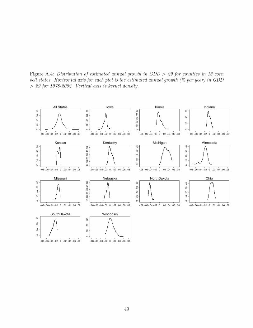
Figure A.4: Distribution of estimated annual growth in GDD > 29 for counties in 13 cornbelt states. Horizontal axis for each plot is the estimated annual growth (% per year) in GDD> 29 for 1978-2002. Vertical axis is kernel density.

010

2030

40

-.08 -.06 -.04 -.02 0 .02 .04 .06 .08

All States

020

4060

80

-.08 -.06 -.04 -.02 0 .02 .04 .06 .08

Iowa

010

2030

4050

-.08 -.06 -.04 -.02 0 .02 .04 .06 .08

Illinois

020

4060

-.08 -.06 -.04 -.02 0 .02 .04 .06 .08

Indiana

2030

4050

60

-.08 -.06 -.04 -.02 0 .02 .04 .06 .08

Kansas

010

2030

4050

-.08 -.06 -.04 -.02 0 .02 .04 .06 .08

Kentucky

510

1520

25

-.08 -.06 -.04 -.02 0 .02 .04 .06 .08

Michigan

010

2030

40

-.08 -.06 -.04 -.02 0 .02 .04 .06 .08

Minnesota

020

4060

80

-.08 -.06 -.04 -.02 0 .02 .04 .06 .08

Missouri

1020

3040

5060

-.08 -.06 -.04 -.02 0 .02 .04 .06 .08

Nebraska

020

4060

80

-.08 -.06 -.04 -.02 0 .02 .04 .06 .08

NorthDakota

010

2030

40

-.08 -.06 -.04 -.02 0 .02 .04 .06 .08

Ohio

1020

3040

-.08 -.06 -.04 -.02 0 .02 .04 .06 .08

SouthDakota

010

2030

-.08 -.06 -.04 -.02 0 .02 .04 .06 .08

Wisconsin

49

Figure A.5: The observed distribution of changes in GDD>29 (in red), compared to 1000distributions generated from data with the same variance but no change in mean (shown ingrey). The left panel is real and simulated changes between 1955-1975, the right panel for1980-2000.

50

A.2 Correlates of trends in extreme heat

Tables A.2 and A.3 investigate the sensitivity of our main long difference results to controllingfor county characteristics. Table A.2 shows that changes from 1980-2000 in GDD>29 arenot strongly correlated with baseline measures of population density, various measures offarm land use, and characteristics of the soil. Table A.3 shows regression coefficients whencontrolling for these variables. Adding controls does not substantially change our results.

Table A.2: Coefficients and p-values of univariate regressions of county characteristics onchange in extreme heat exposure

Coefficient p-ValuePop density 1980 1.96 0.16

Farm area 1978 889.29 0.14

Corn area 1980 273.31 0.31

County area 0.67 0.56

Irrigated area 1982 338.62 0.15

Farm value 1978 16.49 0.15

Percent of soil that is clay -0.04 0.49

Water capacity of soil -0.01 0.60

Percent of soil that is high quality 0.13 0.20

Income per capita 1978 7.59 0.70

Table displays coefficients and p-values from regressions of each county characteristic on change inGDD> 29 from 1980-2000 and state fixed effects. Standard errors for each regression are clustered at thestate level.

A.3 Robustness to outliers

Robustness of our corn yield results to dropping outliers is explored in Table A.4. Pointestimates decline slightly when outliers are dropped – not surprising given that nearly all ofthe outliers experienced both yield declines and large increases in exposure to extreme heat– but coefficients are statistically indistinguishable from estimates on the full sample.

Robustness of the results on alternate adaptation margins to dropping outliers is shownin Table A.5. Here dropping the 5 extreme heat outliers (0.003% of the sample) does havea substantial effect on farm area, on the number of farms, and on farm land values. Whenthese outliers are dropped, extreme heat coefficients on these variables drops by at least60-70% and becomes statistically insignificant. For the reason we focus on the results forthe trimmed sample in the main text.

51

Table A.3: Robustness of long difference results to addition of county control variables(1) (2)

GDD below threshold 0.0000 0.0003∗

(0.0003) (0.0001)

GDD above threshold -0.0046∗∗∗ -0.0043∗∗∗

(0.0010) (0.0008)

Precip below threshold 0.0429∗∗∗ 0.0300∗∗∗

(0.0154) (0.0104)

Precip above threshold 0.0022 0.0028∗∗∗

(0.0015) (0.0009)Observations 1525 1525R squared 0.387 0.637Fixed Effects None StateControls Yes Yes

Table displays long difference regression results from 1980-2000. Standard errors for each regression areclustered at the state level. Temperature threshold is 29◦C and precipitation threshold is 42 cm. Controlvariables are population density in 1980, total farm area in 1978, total corn area in 1980, total county area,irrigated area in 1982, average farm value in 1978, percent of soil that is clay, water capacity of soil,percent of soil that is high quality, and income per capita in 1978. Column 2 also includes state fixedeffects. Asterisks indicate statistical significance at the 1% ∗∗∗,5% ∗∗, and 10% ∗ levels.

Table A.4: Robustness of corn yield results to dropping outliers(1) (2) (3) (4)full trimmed full trimmed

GDD below threshold 0.0002 0.0002 0.0003∗ 0.0002(0.0002) (0.0002) (0.0002) (0.0001)

GDD above threshold -0.0044∗∗∗ -0.0043∗∗∗ -0.0037∗∗∗ -0.0032∗∗∗

(0.0008) (0.0009) (0.0009) (0.0009)

Precip below threshold 0.0297∗∗ 0.0309∗∗ 0.0115∗∗ 0.0117∗∗

(0.0125) (0.0130) (0.0046) (0.0045)

Precip above threshold 0.0034∗∗∗ 0.0034∗∗∗ 0.0029∗∗∗ 0.0030∗∗∗

(0.0008) (0.0008) (0.0007) (0.0007)

Constant 0.2397∗∗∗ 0.2403∗∗∗ 0.2400∗∗∗ 0.2409∗∗∗

(0.0124) (0.0125) (0.0115) (0.0118)Observations 1531 1521 1531 1521R squared 0.610 0.624 0.602 0.617Fixed Effects State State State StateT threshold 29 29 28 28P threshold 42 42 50 50

All regressions use log of corn yields as the dependent variable, and use temperature and precipitationthresholds as indicated at the bottom of the table. Columns 1 and 3 are on the full sample, columns 2 and4 drop the outliers indicated in Figure A.1. Standard errors are clustered at the state level. Asterisksindicate statistical significance at the 1% ∗∗∗,5% ∗∗, and 10% ∗ levels.

52

Tab

leA

.5:

Rob

ust

nes

sof

resu

lts

onal

tern

ate

adap

tati

ons

tore

mov

alof

outl

iers

(1)

(2)

(3)

(4)

(5)

(6)

(7)

(8)

Cor

nar

eaC

orn

are

aC

orn

%C

orn

%F

arm

are

aF

arm

are

a#

farm

#fa

rmG

DD

bel

owth

resh

old

0.00

130.

0010

0.0

003∗∗∗

0.0

003∗∗∗

-0.0

000

-0.0

001

-0.0

001

-0.0

002

(0.0

012)

(0.0

012)

(0.0

001)

(0.0

001)

(0.0

001)

(0.0

001)

(0.0

003)

(0.0

002)

GD

Dab

ove

thre

shol

d-0

.003

8-0

.0005

-0.0

007∗∗

-0.0

009∗∗

-0.0

010∗∗

0.0

000

-0.0

023∗

-0.0

007

(0.0

048)

(0.0

038)

(0.0

003)

(0.0

004)

(0.0

004)

(0.0

004)

(0.0

011)

(0.0

010)

Pre

cip

bel

owth

resh

old

0.04

040.

0264

-0.0

006

-0.0

004

0.0

067

0.0

037

0.0

077∗∗

0.0

021

(0.0

485)

(0.0

637)

(0.0

030)

(0.0

034)

(0.0

043)

(0.0

035)

(0.0

036)

(0.0

029)

Pre

cip

abov

eth

resh

old

-0.0

079

-0.0

051

-0.0

015

-0.0

016

-0.0

001

0.0

007

-0.0

023

-0.0

013

(0.0

067)

(0.0

063)

(0.0

010)

(0.0

010)

(0.0

008)

(0.0

007)

(0.0

032)

(0.0

033)

Con

stan

t-0

.027

3-0

.0130

-0.0

164∗∗∗

-0.0

174∗∗∗

-0.0

649∗∗∗

-0.0

614∗∗∗

-0.1

881∗∗∗

-0.1

836∗∗∗

(0.0

661)

(0.0

687)

(0.0

045)

(0.0

045)

(0.0

079)

(0.0

075)

(0.0

156)

(0.0

157)

Ob

serv

atio

ns

1516

1511

1521

1516

1528

1523

1531

1526

Mea

nof

Dep

Var

iable

0.07

30.0

75

0.0

02

0.0

02

-0.0

69

-0.0

68

-0.2

02

-0.2

02

Rsq

uar

ed0.

642

0.645

0.4

18

0.4

18

0.3

87

0.3

99

0.4

78

0.4

88

Fix

edE

ffec

tsS

tate

Sta

teS

tate

Sta

teS

tate

Sta

teS

tate

Sta

teT

thre

shol

d29

29

29

29

29

29

29

29

Pth

resh

old

4242

42

42

42

42

42

42

Dep

end

ent

vari

able

isd

iffer

ence

inlo

gof

corn

acr

es(C

olu

mn

s1-2

),d

iffer

ence

insh

are

of

agri

cult

ura

lare

ap

lante

dto

corn

(Colu

mn

s3-4

),d

iffer

ence

into

tal

log

farm

area

(Col

um

ns

5-6)

,an

dd

iffer

ence

inlo

gnu

mb

erof

farm

ers

(Colu

mn

s7-8

).A

llre

gre

ssio

ns

are

lon

gd

iffer

ence

sfr

om

1980-2

000,

and

even

nu

mb

ered

regr

essi

ons

hav

eth

esa

mp

letr

imm

edof

ou

tlie

rsin

dic

ate

din

Fig

ure

A.1

.A

llre

gre

ssio

ns

are

wei

ghte

dby

aver

age

agri

cult

ura

lare

afr

om19

78-2

002.

Sta

nd

ard

erro

rsar

ecl

ust

ered

atth

est

ate

leve

l.A

ster

isks

ind

icate

stati

stic

al

sign

ifica

nce

at

the

1%∗∗∗ ,

5%∗∗

,an

d10%∗

leve

ls..

53

A.4 Choice of time period

Our main specification focuses on changes in climate and yields of the 1980-2000 period. Wefocus on this period for a few reasons. First, relative to earlier periods, and as shown in FigureA.7, global warming had begun in earnest over this period, and counties had experiencedon average much more warming. Importantly, many more counties had experienced at least1C warming over the period, making this period more representative of the warming thatclimate models predict will occur over the next few decades and thus a better baseline withwhich to project future impacts. Second, prior to 1980, scientific opinion was relatively splitas to whether the future climate would be cooler or warmer than the current climate, andin fact there was significant concern about “global cooling” (e.g. Gwynne (1975)). Growingscientific and public recognition of “global warming” during the 1980’s and 1990’s – i.e. arecognition that increasing greenhouse gas emissions would lead to future warming – againmakes this period more relevant for projecting future impacts because there was recognitionthat the climate was warming and would continue to warm.

Nevertheless, Figure 4 directly compares our benchmark 1980-2000 estimate to estimatesusing alternate time periods and differencing lengths, and shows that these alternate es-timates are largely indistinguishable from our main estimate. Figure A.6 displays pointestimates and their confidence intervals from each of these regressions (rather than compar-isons with the 1980-2000 estimate); all of these estimates are negative, and in only 8 out of39 cases do we fail to reject no effect of extreme heat on corn yields.

As a final robustness test on our choice of time period, we vary the length of the endpointsover which our two periods are averaged. We begin with our 1980-2000 period, and averageour endpoints over ten years instead of five – i.e. the long difference is now 1995-2005average minus 1975-1985 average. We include in the sample any counties that reportedgrowing corn in at least one year in both periods, or restrict the sample to counties thatgrew corn in all years in both averaging periods. Results are given in Columns 1 and 2 ofTable A.6. Coefficients on extreme heat in both specifications are slightly more negativethan our baseline estimates and highly significant.

Finally, we utilize our full 1950-2005 sample, split it into 28-year periods (1950-1977 and1978-2005), average both climate and crop yields within each period, difference these aver-ages, and then run our basic long differences specification on these two time periods. Thisis equivalent to smoothing our data with a 28-year running mean, and then differencing be-tween the years 1991 and 1964. We similarly restrict the sample to include either all countiesreporting growing corn in at least one year in both periods (column 3), or successively limitthe sample to counties with at least 40, 50, or 56 observations (columns 4-6).

The coefficient on GDD above 29C is again large, negative, and highly significant acrossall specifications. Point estimates are in fact substantially more negative than for our baseline1980-2000 period. One explanation for this is that farmers have become less sensitive totemperature over time, with our main 1980-2000 specification focusing on a later (and thusless sensitive) period. But both Figure 4 and Figure A.8 (see discussion below) show thatthere is little evidence that temperature sensitivities have declined over time. We can alsorun the panel model for the full 1950-2005 period (shown in column 7 of Table A.6), andwe find that the panel coefficient on extreme heat is somewhat more negative that for the1980-2000 period but not substantially so. An alternate explanation is that if measurement

54

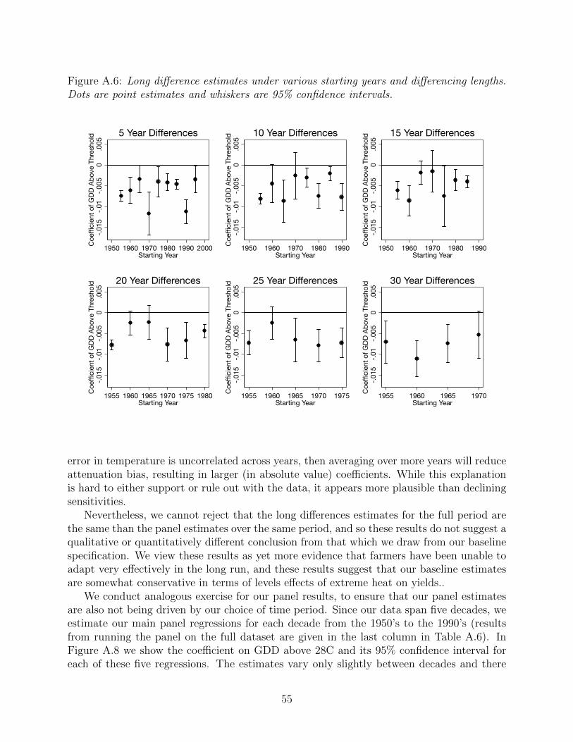
Figure A.6: Long difference estimates under various starting years and differencing lengths.Dots are point estimates and whiskers are 95% confidence intervals.

-.015

-.01

-.005

0.0

05C

oeffi

cien

t of G

DD A

bove

Thr

esho

ld

1950 1960 1970 1980 1990 2000Starting Year

5 Year Differences

-.015

-.01

-.005

0.0

05C

oeffi

cien

t of G

DD A

bove

Thr

esho

ld

1950 1960 1970 1980 1990Starting Year

10 Year Differences

-.015

-.01

-.005

0.0

05C

oeffi

cien

t of G

DD A

bove

Thr

esho

ld

1950 1960 1970 1980 1990Starting Year

15 Year Differences

-.015

-.01

-.005

0.0

05C

oeffi

cien

t of G

DD A

bove

Thr

esho

ld

1955 1960 1965 1970 1975 1980Starting Year

20 Year Differences

-.015

-.01

-.005

0.0

05C

oeffi

cien

t of G

DD A

bove

Thr

esho

ld

1955 1960 1965 1970 1975Starting Year

25 Year Differences

-.015

-.01

-.005

0.0

05C

oeffi

cien

t of G

DD A

bove

Thr

esho

ld

1955 1960 1965 1970Starting Year

30 Year Differences

error in temperature is uncorrelated across years, then averaging over more years will reduceattenuation bias, resulting in larger (in absolute value) coefficients. While this explanationis hard to either support or rule out with the data, it appears more plausible than decliningsensitivities.

Nevertheless, we cannot reject that the long differences estimates for the full period arethe same than the panel estimates over the same period, and so these results do not suggest aqualitative or quantitatively different conclusion from that which we draw from our baselinespecification. We view these results as yet more evidence that farmers have been unable toadapt very effectively in the long run, and these results suggest that our baseline estimatesare somewhat conservative in terms of levels effects of extreme heat on yields..

We conduct analogous exercise for our panel results, to ensure that our panel estimatesare also not being driven by our choice of time period. Since our data span five decades, weestimate our main panel regressions for each decade from the 1950’s to the 1990’s (resultsfrom running the panel on the full dataset are given in the last column in Table A.6). InFigure A.8 we show the coefficient on GDD above 28C and its 95% confidence interval foreach of these five regressions. The estimates vary only slightly between decades and there

55

Table A.6: Long differences regressions with endpoints averaged over longer periods.(1) (2) (3) (4) (5) (6) (7)

1980-2000 1980-2000 1950-2005 1950-2005 1950-2005 1950-2005 panel 50-05GDD below 0.0000 0.0000 0.0008∗∗ 0.0008∗∗ 0.0009∗∗ 0.0010∗∗ 0.0004∗∗∗

(0.0002) (0.0002) (0.0003) (0.0003) (0.0003) (0.0003) (0.0001)

GDD above -0.0050∗∗∗ -0.0047∗∗∗ -0.0090∗∗∗ -0.0091∗∗∗ -0.0102∗∗∗ -0.0096∗∗ -0.0065∗∗∗

(0.0010) (0.0011) (0.0025) (0.0027) (0.0030) (0.0034) (0.0006)

Precip below 0.0234∗∗∗ 0.0245∗∗∗ 0.0480∗∗∗ 0.0460∗∗∗ 0.0457∗∗∗ 0.0450∗∗∗ 0.0172∗∗∗

(0.0045) (0.0045) (0.0047) (0.0049) (0.0049) (0.0046) (0.0022)

Precip above 0.0026 0.0027 0.0021 0.0023 0.0022 0.0020 -0.0020∗∗∗

(0.0019) (0.0019) (0.0033) (0.0035) (0.0036) (0.0039) (0.0003)

Constant 0.2805∗∗∗ 0.2809∗∗∗ 0.5206∗∗∗ 0.5232∗∗∗ 0.5237∗∗∗ 0.5117∗∗∗ 2.7418∗∗∗

(0.0074) (0.0080) (0.0101) (0.0110) (0.0123) (0.0132) (0.2234)Observations 1950 1451 2241 1711 1262 956 107290Mean of Dep Var.e 0.31 0.31 0.57 0.57 0.58 0.57 4.42R squared 0.627 0.670 0.687 0.719 0.722 0.734 0.821Period 1 years 1975-1985 1975-1985 1950-1977 1950-1977 1950-1977 1950-1977Period 2 years 1995-2005 1995-2005 1978-2005 1978-2005 1978-2005 1978-2005Min. yrs in sample 2 All 2 40 50 All Any

All regressions use log of corn yields as the dependent variable, and use the 29C temperature and 42cmprecipitation thresholds. The sample period is either 1975-2005 (columns 1-2) or 1950-2005 (columns 3-7),with endpoints averaged over the two different periods given in the bottom of the table. As indicated inthe last line of the table, samples either include counties that report at least one year of growing corn inboth periods (columns and 3), counties that grew corn in all years in the sample (columns 2 and 6), orcounties that grew corn in at least 40 or 50 years of the 56-year sample (columns 4 and 5). The final model(column 7) is a panel model over the full 1950-2005 period. Standard errors are clustered at the state level,and asterisks indicate statistical significance at the 1% ∗∗∗,5% ∗∗, and 10% ∗ levels.

56

Figure A.7: Distribution of the change in average growing season temperature across oursample counties, for the period 1960-1980 (dotted line) or the period 1980-2000 (solid line).

−1.0 −0.5 0.0 0.5 1.0 1.5

0.0

0.2

0.4

0.6

0.8

1.0

1.2

1.4

Change in Temperature (C)

Den

sity

1960−1980

1980−2000

is no clear pattern suggesting that corn yields have become less sensitive to short-termdeviations in weather over time.

While this unchanging sensitivity of yield to extreme heat over time could be interpretedas additional evidence of a lack of adaptation (as in Schlenker and Roberts (2009)), we notethat whether responses to short-run variation have changed over time is conceptually distinctfrom whether farmers have responded to long-run changes in average temperature. In par-ticular, there is no reason to expect farmers to respond similarly to these two different typesof variation. Indeed, farmers could adapt completely to long-run changes in temperaturesuch that average yields do not change – e.g. by adopting a new variety that on averageperforms just as well in the new expected temperature as the old variety did under the oldaverage temperature – but still face year-to-year variation in yield due to random deviationsin temperature about its new long-run average. As such, we view this exercise more as atest of the robustness of the panel model than as evidence of (a lack of) adaptation per se.

A.5 Measurement error

As discussed in the main text, one concern is that fixed effects estimators are more likely thanlong differences estimates to suffer attenuation bias if climate variables are measured witherror. Following Griliches and Hausman (1986), we compare fixed effectsand first differenceestimates with random effects estimates, with the expectation that if measurement error inour climate variables is a problem, then estimates from a random effects estimation shouldbe larger in absolute value than the fixed effects estimates which in turn should be largerthan estimates using first differences.

57

Figure A.8: Panel estimates of the effect of extreme heat on log corn yields by decade. Figureshows point estimate and 95% confidence interval for regressions run separately for eachdecade. The black line is the coefficient on extreme heat from our baseline panel regression(Column 3 in Table 1) . All regressions include county and time fixed effects and are weightedby average corn area in the county during the relevant decade, with errors clustered at thestate level.

0-.0

02-.0

04-.0

06-.0

08C

oeffi

cien

t of G

DD A

bove

Thr

esho

ld

1950-59 1960-69 1970-79 1980-89 1990-99Decade

Table A.7 presents the results of a horse race between these three estimators. The firstcolumn presents unweighted fixed effects estimates. The random effects estimates in Column2 are remarkably similar to the fixed effects estimates. The main coefficient of interest forGDD above 28◦ is smaller in absolute value by a modest 7%. Column 3 shows that the firstdifference estimator also produces a very similar effect of increases in temperatures above 28◦

on yields. Results suggest that measurement error is not responsible for the lack of differencebetween fixed effects estimators and long differences that we observe in the data.

A.6 Functional Form

Our use of growing degree days to capture nonlinearities is primarily motivated by resultsfrom the agronomy literature suggesting that plant growth increases linearly with temper-ature up to a certain threshold level, and then declines with further temperature increases.Figure 3 in the main text shows that our results produce this relationship. Our piecewiselinear approximation will be misspecified in the presence of strong nonlinearities within theranges from 0-29 and 29 and above. Schlenker and Roberts (2009) show that the piecewiselinear relationship achieved with growing degree days estimates that use either a higher orderpolynomial or a set of temperature bins measuring the days of exposure to various temper-ature ranges. These results strongly suggest that use of growing degree days is not affected

58

Table A.7: Understanding measurement error through the comparison of panel estimators(1) (2) (3)

Fixed Effects Random Effects First DifferenceGDD below threshold 0.0004∗∗∗ 0.0003∗∗∗ 0.0003∗∗∗

(0.0001) (0.0001) (0.0001)

GDD above threshold -0.0045∗∗∗ -0.0042∗∗∗ -0.0045∗∗∗

(0.0005) (0.0005) (0.0004)

Precip below threshold 0.0045∗∗ 0.0040∗∗ 0.0054∗∗∗

(0.0018) (0.0017) (0.0018)

Precip above threshold -0.0011∗ -0.0011 -0.0009(0.0006) (0.0007) (0.0006)

Constant 3.2154∗∗∗ 3.6483∗∗∗ 0.0703∗∗

(0.2877) (0.1648) (0.0343)Observations 48465 48465 45405R squared 0.463 0.494Fixed Effects Cty, Yr Yr YrT threshold 28 28 28P threshold 50 50 50

All regressions use log of corn yields as the dependent variable. All regressions are unweighted. Standarderrors are clustered at the state level. Asterisks indicate statistical significance at the 1% ∗∗∗,5% ∗∗, and10% ∗ levels.

by misspecification due to nonlinearity.Nevertheless, we re-estimate both our main panel and long difference specifications using

three degree bins. In both models we include the same functions of precipitation as wereincluded in the main specifications. Figure A.9 shows the results. Both the panel andlong difference specifications using temperature bins produce similar results to those usinggrowing degree days, consistent with Schlenker and Roberts (2009). Our use of growingdegree days does not seem to misrepresent the relationship between temperature and yields.

A.7 Effects on soy productivity

Estimates of the impact of extreme heat on (log) soy yields are shown in Figure A.10. Thehorizontal line in each panel is the 1978-2002 panel estimate of β2 for soy which is -0.0047.The thresholds for temperature and precipitation are 29◦ and 50 cm, which are those thatproduce the best fit for the panel model. The average response to extreme heat across the39 estimates is -0.0032, giving a point estimate of longer run adaptation to extreme heat ofabout 30%. This estimate is slightly larger but of similar magnitude to the corn estimate,and we are again unable to reject that the long differences estimates are different than thepanel estimates. As for corn, we conclude that there is limited evidence for substantialadaptation of soy productivity to extreme heat.

59

Figure A.9: Relationship between corn yields and temperature. Estimates represent thechange in log corn yield under an additional day of exposure to a given ◦C temperature, rel-ative to a day spent at 0-3◦C. Estimates of 3◦C temperature bins are used for long differenceand panel versions of binned regressions. Dots represent midpoints of bins. GDD regressionsare identical to those in Figure 3 of the main text. The shaded area is the confidence intervalof the long difference estimates where temperature is measured with GDD.

-.08

-.06

-.04

-.02

0.0

2N

orm

aliz

ed p

redi

cted

log

yiel

ds

0 10 20 30 40Temperature (C)

LD:GDD Panel:GDDLD:Bin Panel:Bin

A.8 Revenues and profits

A basic concern with our crop yield results is that they could hide alternate adjustments thathelp farmers maintain profitability in the face of a changing climate. The US AgriculturalCensus, conducted roughly every 5 years, contains data on overall farm revenues and expensesfor the year in which the census is conducted. A basic measure of profits for a given year canbe constructed by differencing these two variables (i.e. profits2000 = revenues2000 - costs2000for years in which data are available, and and this approach as recently been used in similarsettings (Deschenes and Greenstone, 2007).

We choose not to focus on such a profit measure for two reasons. The first is a concern thatcosts are not fully measured, and that unmeasured costs might respond to climate shocksin a way that would bias the above profit measure. In particular, expense data do notappear to include the value of own or family labor, which could respond on the intensive orextensive margin in the face of a drought or heat event (e.g. if a crop fails and is replanted).32

The second concern is that both costs and revenues will likely respond to annual variation

32In recent years, the value of own labor appears to represent about 10% of operating costs for corn, basedon cost estimates available at http://www.ers.usda.gov/data-products/commodity-costs-and-returns.aspx.Hired labor expenditures are minimal for corn.

60

Figure A.10: Effects of extreme heat on soy yields under various starting years and dif-ferencing lengths, as compared to the point estimate from a 24-year panel estimated over1978-2002 displayed by the horizontal line in each figure panel.

-.015

-.01

-.005

0.0

05C

oeffi

cien

t of G

DD A

bove

Thr

esho

ld

1950 1960 1970 1980 1990 2000Starting Year

5 Year Differences

-.015

-.01

-.005

0.0

05C

oeffi

cien

t of G

DD A

bove

Thr

esho

ld

1950 1960 1970 1980 1990Starting Year

10 Year Differences

-.015

-.01

-.005

0.0

05C

oeffi

cien

t of G

DD A

bove

Thr

esho

ld

1950 1960 1970 1980 1990Starting Year

15 Year Differences

-.015

-.01

-.005

0.0

05C

oeffi

cien

t of G

DD A

bove

Thr

esho

ld

1955 1960 1965 1970 1975 1980Starting Year

20 Year Differences

-.015

-.01

-.005

0.0

05C

oeffi

cien

t of G

DD A

bove

Thr

esho

ld

1955 1960 1965 1970 1975Starting Year

25 Year Differences

-.015

-.01

-.005

0.0

05C

oeffi

cien

t of G

DD A

bove

Thr

esho

ld

1955 1960 1965 1970Starting Year

30 Year Differences

in climate, but data are only available for 5-year snapshots. Given that our differencingapproach seeks to capture change in average farm outcomes over time, differencing two ofthese snapshots might provide a very noisy measure of the overall change in profits.

Regressions appear to confirm that profit measures are quite noisy. Agricultural censusdata on expenditures and revenues are available in 1978, 1982, 1987, 1992, 1997, and 2002.We construct a measure of the change in log profits as:

∆logprofits1980−2000 = ln(profit1997 + profit2002)/2− ln(profit1978 + profit1982)/2 (14)

When we re-estimate our main specification with ∆logprofits1980−2000 as the dependentvariable, the coefficient on extreme heat using the untrimmed sample is β2 = −0.0013,with 95% CI of [-0.010, 0.007], and using the trimmed sample we have β2 = −0.0054, with95% CI of [-0.014,0.003]. This means we can’t reject that there is no effect on profits, andsimilarly can’t reject that the effect of extreme heat on profits is a factor of 3 larger (andmore negative) than the effect on corn yields – i.e. that each additional day of exposure

61

to temperatures above 29C reduced annual profits by 1.4%. This does not provide muchinsight on the relationship between extreme heat exposure and profitability.

We take two alternate approaches to exploring profitability impacts that help to addressthese measurement issues. The first is to construct a measure of revenues using annual yielddata, which we multiply by annual data on state-level prices to obtain revenue-per-acre fora given crop. Summing up these revenues across crops then provides a reasonable measureof annual county-level crop revenues, which will be underestimated to the extent that notall contributing crops are included. The effect of climate variation on this revenue measureis given in the main text, and we find minimal difference between panel and long differenceestimates of impacts on expenditures.

Our second approach proceeds with the available expenses data from the ag census toexamine the impact of longer-run changes in climate on different input expenditures, wherewe attempt to capture changes in average expenditures by averaging two census outcomesnear each endpoint and then differencing these averaged values.33 As shown in Table A.8,we find little effect of long-run trends in climate on expenditures on fertilizer, seed, chemical,and petroleum. While we do not wish to push these expenditure data too far given the noisyway in which the long differences are constructed, we interpret these as further evidencethat yield declines are economically meaningful and not masking other adjustments on theexpenditure side that somehow reduce profit losses.

Table A.8: Effects of Climate Variation on Input Expenditures(1) (2) (3) (4)

Fertilizer Seed Chemicals PetroleumGDD below threshold 0.0005 0.0008∗∗ 0.0011∗ 0.0002

(0.0004) (0.0004) (0.0006) (0.0004)

GDD above threshold -0.0007 -0.0009 -0.0001 -0.0009(0.0015) (0.0013) (0.0034) (0.0011)

Precip below threshold 0.0141 -0.0105 0.0392∗∗∗ -0.0016(0.0229) (0.0125) (0.0115) (0.0087)

Precip above threshold -0.0016 -0.0021 0.0004 0.0010(0.0019) (0.0024) (0.0036) (0.0019)

Constant 0.3215∗∗∗ 0.7295∗∗∗ 0.6993∗∗∗ 0.0281(0.0276) (0.0217) (0.0338) (0.0237)

Observations 1528 1519 1523 1518R squared 0.532 0.313 0.460 0.258Fixed Effects State State State StateT threshold 29 29 29 29P threshold 42 42 42 42

Dependent variable is difference in log of input expenditure per acre. All regressions are long differencesfrom 1980-2000. All regressions are weighted by average agricultural area between 1978-1982. Standarderrors are clustered at the state level. Asterisks indicate statistical significance at the 1% ∗∗∗,5% ∗∗, and10% ∗ levels.

33As with the profit measure described above, the change in fertilizer expenditures over the period areconstructed as: ∆fertilizer expenditure1980−2000 = (fert1997 + fert2002)/2 - (fert1978 + fert1982)/2

62

A.9 Exit from agriculture

As an extension to our basic long difference results on how the number of farms changein response to climate variation, we adopt an empirical strategy similar to that of Horn-beck (2012). We use the six agricultural censuses from 1978-2002 to estimate whether thenumber of farms grew differently between areas that were differentially exposed to extremeheating from 1970-1980. We first take the difference between average annual GDD above29◦ from 1976-1980 and average annual GDD above 29◦ from 1966-1970. We then defineextreme heating as an indicator variable for this difference being above a certain value. Theeconometric specification is,

ln(farms)ist − ln(farms)is1978 = βt ∗ Extremeheatis + αst + εist, (15)

where Extremeheatis is an indicator variable for a large change in GDD above 29. Animportant note is that the census defines a farm to be any place where at least $1000in agricultural products was sold during that year. Table A.9 reports estimates with andwithout state-specific time fixed effects. The state specific time-effect eliminates all state-specific factors varying over time. For instance, if heating was more heavily concentrated insome states and those states had different policies over time, the state-specific time effectswould control for this correlation. We also show two different definitions of extreme heat.In the first definition it is defined as an indicator for an increase in GDD above 29◦ of10 or more. This results in approximately 48% of counties being classified as having beenexposed to heating. The second definition uses a stricter cutoff of 20. This results in 28% ofcounties being classified as exposed to heating. Each coefficient βt measures the predictedpercentage difference in the number of farms in year t between the counties that warmedfrom 1970-1980 and those that did not. For instance in Column 2, the number of farms in1982 is predicted to be 2.75% lower in counties that heated substantially from 1970-1980.This predicted difference increases to 3.5% in 1987. The predicted difference in the numberof farms generally becomes smaller in the later years of 1997 and 2002 which is consistentwith some longer term adjustments back towards pre-warming degree of farming activity.This interpretation must be made with caution given the large standard errors in these years.The pattern of coefficients suggests that simply not farming may be an important immediateadaptation to climate change.

A.10 Additional evidence on selection

The potential of exit from agriculture and migration as responses to climate change highlightsan important potential issue with our estimates of the effects of long-term climate trends onyields. If exit/migration is selective, then the appearance of a lack of adaptation in the datacould be due to a selection effect where the most productive farmers recognize the changingclimate and leave agriculture. In this case the appearance of a lack of adaptation in thedata could be due to the change in the ability of the farming population that results fromclimate change. This possibility would become especially problematic if farmers that weremore productive and had access to better quality land also had a larger opportunity costof being in farming. If selection of this type is driving our estimates then we should see

63

Table A.9: Estimated Differences in Log Number of Farms by Amount of WarmingExtreme Heat=Change GDD > 10 Extreme Heat=Change GDD > 20

(1) (2) (3) (4)

1982*Extreme Heating -0.0585∗∗∗ -0.0275∗∗ -0.0741∗∗∗ -0.0230∗∗∗

(0.0177) (0.0107) (0.0231) (0.0057)

1987*Extreme Heating -0.0579∗∗∗ -0.0352∗∗ -0.0727∗∗∗ -0.0455∗∗

(0.0190) (0.0166) (0.0205) (0.0216)

1992*Extreme Heating -0.0351 -0.0396 -0.0460∗∗ -0.0430∗∗

(0.0223) (0.0240) (0.0191) (0.0179)

1997*Extreme Heating 0.0051 -0.0155 -0.0016 -0.0221(0.0296) (0.0318) (0.0216) (0.0171)

2002*Extreme Heating 0.0174 -0.0169 0.0045 -0.0617∗

(0.0351) (0.0299) (0.0352) (0.0318)Observations 12120 12120 12120 12120Mean of Dep Variable -0.13 -0.13 -0.13 -0.13R squared 0.617 0.681 0.618 0.681State by Year Fixed Effects No Yes No Yes

Data are for US counties east of the 100th meridian. Dependent variable in all specifications is differencebetween log number of farms in year t and log number of farms in 1978. Coefficients represent estimateddifferences in log number of farms between counties that experienced extreme heating from 1970-1980 andthose that did not. Extreme heating defined as indicator for increases in GDD above 29 greater than cutoffvalue of 10 (Columns 1-2) or 20 (Columns 3-4). All regressions are weighted by county farm area in 1978.Standard errors are clustered at the state level. Asterisks indicate statistical significance at the 1% ∗∗∗,5%∗∗, and 10% ∗ levels.

characteristics that are correlated with productivity changing differentially between placesthat heated and those that did not. In Table A.10 we regress the percentage of farms owingmore than $20,000 in equipment on our same climate variables. Since the percentage offarms owning valuable equipment is positively correlated with yields, if selection is drivingour results we should expect to see a large decrease as a response to increases in extremetemperatures. The results are not consistent with this story. The long differences estimate isnegative, but small and not statistically significant from zero. The panel estimate is positive,small in magnitude and marginally statistically significant. While we obviously can not fullyrule out selective migration, these regressions are suggestive that it is not driving our yieldresults.

A.11 Why no adaptation

As described in the main text, Table A.11 provides some evidence that participation in thegovernment insurance program by 2000 was higher in counties who saw large increases inexposure to harmful temperatures (GDD>29C) over the previous two decades, and lower incounties that saw increase in exposure to generally helpful temperatures (GDD0-29C) overthe same period.

64

Table A.10: Effects of climate variation on equipment ownership.(1) (2)

Diffs, 1978-1997 Panel, 1978-2002GDD below threshold 0.0087 -0.0067∗∗∗

(0.0152) (0.0019)

GDD above threshold -0.0178 0.0221∗

(0.0318) (0.0109)

Precip below threshold 0.2114 0.0608(0.1470) (0.0499)

Precip above threshold 0.0524 0.0760∗∗∗

(0.1147) (0.0250)

Constant 9.9251∗∗∗ 74.5041∗∗∗

(0.9928) (6.0013)Observations 1531 7645Mean of Dep Variable 10.50 59.01R squared 0.321 0.324Fixed Effects State Cty, YrT threshold 28 28P threshold 50 50

Dependent variable in Column 1 is the change in the percentage of farms with more than 20K USD inequipment from 1978 to 1997. Dependent variable in Column 2 is the percentage of farms owningequipment valued at more than 20,000 USD. Long differences regressions are weighted by average farmacres between 1978 and 1982. Panel regressions weighted by average farm acres from 1978-2002. Standarderrors are clustered at the state level. Asterisks indicate statistical significance at the 1% ∗∗∗,5% ∗∗, and10% ∗ levels.

A.12 Climate change projections

We derive projected changes in corn productivity due to climate change by combiningour long differences estimates of the the historical response of corn productivity to cli-mate with climate projections from 18 general circulation models that have contributed toWorld Climate Research Programs Coupled Model Intercomparison Project phase 3 (WCRPCMIP3). Our main projections use the A1B emissions scenario, reported by 18 climatemodels in the CMIP3 database: CCMA, CNRM, CSIRO, GFDL0, GFDL1, GISS.AOM,GISS.EH, GISS.ER, IAP, INMCM3, IPSL, MIROC.HIRES, MIROC.MEDRES, ECHAM,MRI, CCSM, PCM, and HADCM3. For more on these models and their application,see Auffhammer et al. (2013) and Burke et al. (2013). The A1B scenario is considereda “medium” emission scenario, and represents a world experiencing “rapid and successfuleconomic development” and a “balanced mix of energy technologies” (Nakicenovic et al.,2000). We choose to explore outcomes under only one emissions scenario both to simplifythe results, and because emissions scenarios diverge much less by mid-century than they doby the end of the century, meaning our results are less sensitive to the choice of emissionsscenario than end-of-century projections. Finally, following the climate literature, we adopta “model democracy” approach and assume projections from all models are equally validand should be weighted equally (Burke et al., 2013).

65

Table A.11: Insurance take-up in 1998-2002 as a function of changes in GDD and precipita-tion over 1980-2000.

(1) (2) (3) (4)% Acreage Enrolled log Acres Enrolled Policies Sold Total Premiums

GDD below threshold -0.0014∗∗ -0.0011 -0.5287 -1.1756(0.0006) (0.0007) (0.4667) (0.7919)

GDD above threshold 0.0023 0.0030 3.0773∗ 4.0766(0.0027) (0.0026) (1.7300) (2.8459)

Precip below threshold 0.0301 0.0339∗∗ -21.1714∗ -10.0991(0.0186) (0.0130) (12.0231) (25.2031)

Precip above threshold -0.0028 -0.0025 -1.7970 -4.4901(0.0070) (0.0043) (3.8934) (7.4896)

log corn area 1.0180∗∗∗

(0.0470)

Constant 0.9047∗∗∗ -0.4625 299.4046∗∗∗ 498.8283∗∗∗

(0.0440) (0.4534) (29.1904) (49.8694)Observations 1529 1529 1529 1529R squared 0.178 0.940 0.562 0.554Mean Dep. Var. 0.815 9.329 271.227 428.441

The outcome variables are given at the top of each column. Total premiums paid (column 4) are inthousands of dollars. All regressions include state fixed effects, with standard errors are clustered at thestate level. Asterisks indicate statistical significance at the 1% ∗∗∗,5% ∗∗, and 10% ∗ levels.

The resolution of these general circulation models is roughly 2.8◦x2.8◦ (about 300km atthe equator), and we map each county in our sample to its corresponding grid cell in theclimate model grids. We derive estimates of climate change by mid-century by calculat-ing model-projected changes in temperature (C) and precipitation (%) between 2040-2059and 1980-1999, and then adding (for temperature) or multiplying (for precipitation) thesechanges to the observed record of temperature and precipitation in a given county. For tem-perature, because our main variable of interest is growing degree days, this requires addingmonthly predicted changes in temperature in a given county to the daily time series series inthat county, recomputing growing degree days under this new climate, and calculating thedifference between baseline and future growing degree days.

Projections assume a fixed growing season (Apr 1 - Sept 30) and no large shifts in the areawhere corn is grown within the US. Area-weighted changes in temperature and precipitationover US corn area are shown in Figure A.11. The variation in temperature changes overour 1980-2000 study period span the lower third of the range of model-projected averagetemperature changes by 2050, and the variation in changes in precipitation in our samplefully span the range of projected average precipitation changes by 2050.

66

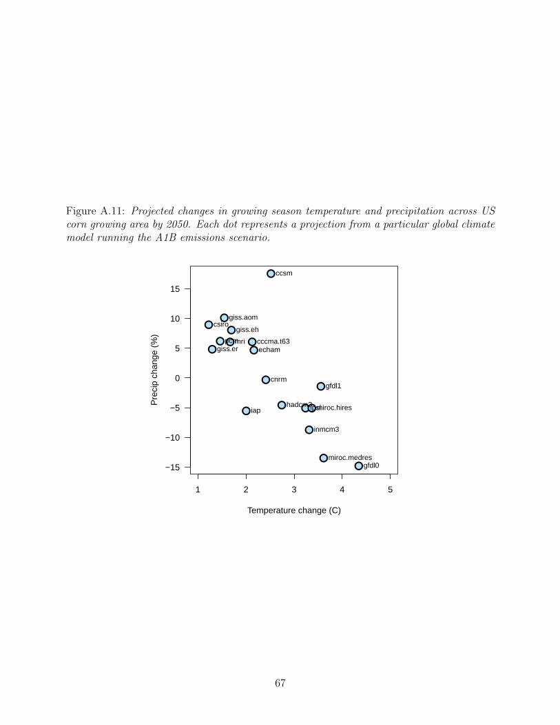
Figure A.11: Projected changes in growing season temperature and precipitation across UScorn growing area by 2050. Each dot represents a projection from a particular global climatemodel running the A1B emissions scenario.

●

●

●

●

●

●

●

●

●

●

●●

●

●●

●

●

●

1 2 3 4 5

−15

−10

−5

0

5

10

15

Temperature change (C)

Pre

cip

chan

ge (

%)

cccma.t63

cnrm

csiro

gfdl0

gfdl1

giss.aom

giss.eh

giss.er

iap

inmcm3

ipslmiroc.hires

miroc.medres

echammri

ccsm

pcm

hadcm3

67