a system for forecasting chilean cash demand–the …

40

BANCO CENTRAL DE CHILE

A SYSTEM FOR FORECASTING CHILEAN CASH DEMAND–THE ROLE OF FORECAST COMBINATIONS

Camila Figueroa S.*Michael Pedersen

I. INTRODUCTION

Several studies are concerned with analyzing the demand for money and the focus is usually on broad measures such as M1 and M3.1 There are fewer studies focused on the demand for cash even though plausible forecasts of future demand for banknotes and coins are important inputs for efficient stock management, a concern of the monetary authorities in several countries. Cash stock management is no trivial issue, as the monetary authorities have to balance the costs of having too large a stock of cash against the risk of not being able to supply what the economy demands. The cost of the latter is, however, not directly measurable. The investigation in the present paper pursues the quest of finding suitable models for predicting the changes in the stock of outstanding cash in Chile as well as for individual denominations of banknotes and coins. These forecasts may help to plan future orders and deliveries and, hence, to optimize the stock of cash the Central Bank of Chile (CBCh) needs to maintain.2

More concretely, we extend the work of Chumacero et al. (2008), henceforth CPV, by presenting a new system for forecasting the demand for cash in Chile, which contains some new time series models as well as some that include fundamental variables.3 Furthermore, not only the forecast performance for the individual denominations is evaluated, but also the one with respect to the change in total stock of cash in circulation. This latter may be useful when experts apply judgment to the models’ forecasts. In contrast to other studies on cash demand forecasts, we present a number of models and can, thus, take advantage of combining the forecasts, which to the best of our knowledge has never been done earlier in the related literature.

1 Surveys of the money demand literature are offered by e.g. Barnett et al. (1992) and Duca and VanHoose (2004).

2 The issue of minimizing inventory costs is a complex one, and the present research paper merely presents a number of econometric models, which can be utilized in the forecasting process to improve the estimations of future demand.

3 The models based on fundamentals are inspired by Baumol (1952) and Tobin (1956) who find a relation between money demand, activity and the opportunity cost of holding money, i.e., the interest rate. Even though the elasticities in the Baumol-Tobin model may be better captured by broader measures of money, in the present paper we estimate them between nominal variables with respect to the demand for cash. Briglevics and Schuh (2014) employ an extended version of the Baumol-Tobin model (Sastry, 1970) that allows for the use of credit cards to study U.S. consumer demand for cash.

It is difficult to make predictions, especially about the future.(Danish proverb)

* Economic Research Department, Central Bank of Chile. Emails: [email protected]; [email protected]

41

ECONOMÍA CHILENA | VOLUMEN 22, Nº2 | AGOSTO 2019

A priori one might expect that models based on fundamental variables would perform better when the money supply is endogenous, whereas time series models might be more appropriate for economies where it is exogenous. In the case of Chile, and this is probably the case for other economies as well, the supply of banknotes is best described as being exogenous during the period investigated in the sense that not all of the banks’ demand for bills has been supplied all the time. On the other hand, given this fact, the commercial banks may inflate their demand in order to obtain the quantity of bills they desire given the restriction they expect the central bank to impose. Hence, in practice the Chilean supply may be characterized as being exogenous during the period analyzed, but with an important endogenous component.

The evidence from the forecasting exercises suggests that the average forecasts, i.e. the average of the forecasts of all the models employed, performs quite well with respect to the total stock of circulating cash, but individual models and sub-combinations frequently make better predictions of the denominations. With respect to aggregate cash in circulation, some additional experiments reveal that precise forecasts of the fundamental variables may help to predict the stock on the three-year horizon and projections with aggregate observations perform better than the sum of the single denomination forecasts.

Amongst the existing studies of currency demand, only a few are concerned with forecasting.4 Gerst and Wilson (2011) estimate models for each dollar bill denomination up to US$100 as well as aggregate demand with models that include information of regulation / policy, domestic and international macroeconomic variables, demographic trends, and technology and consumer taste. They also include seasonal dummies in the model and with a pseudo out-of-sample forecast exercise, using actual values of the exogenous variables, they argue that the model does a “fairly good job of predicting.” To predict the demand for various denominations of Norwegian coins and notes, Vale (2015) estimates vector error correction models including as exogenous variables point-of-sale consumption by the household sector (goods and services for which consumers are likely to consider using notes and coins), number of terminals for electronic funds transfer at points of sales, the central bank’s interest rate and some specific dummies including seasonal ones. He argues that these models out-of-sample forecast “reasonably well” over the horizon of eight quarters. In a recent study, Miller (2017) applies an error correction model to forecast the demand for banknotes in the UK. The variables included are the interest rate, exchange rates, nominal consumption, ATMs, number of bank branches, self-

4 Recent literature on currency demand includes the studies of Doyle (2000): Foreign demand for currencies of the U.S., Germany, and Switzerland; Khamis and Leone (2001) on real currency demand in Mexico after its financial crisis in 1994; Akinci (2003) on currency circulation in Turkey; Fischer et al. (2004) on circulation of euros; Amromin and Chakravorti (2009) on demand for small currency denominations in 13 advanced economies; Columba (2009) on transaction technology and demand for currency and M1 in Italy; Cusbert and Rohling (2013) on currency demand in Australia during the recent international financial crisis; Bagnall et al. (2014) conduct a comparison of consumer cash usage in seven industrialized countries; Briglevics and Schuh (2014) on U.S. consumer demand for cash; Dunbar (2014) on currency demand and demographics in Canada; and Bartzsch et al. (2015) investigate demand for euro banknotes in Germany.

42


employment, and the number of regular payments made in cash. Variables that turned out not to be important are the unemployment rate, the proportion of workers born in Eastern Europe, estimates of the shadow economy, effective exchange rate, official foreign holdings of sterling, VIX, sterling-dollar volatility, tourist expenditure, number of state benefit payments per person and the number of students in the UK. For Chile, CPV employ autoregressive models and autoregressive distributed lag models to estimate demands for real stock (deflated by the consumer price index) of coins and notes. The explanatory variables are monthly data of GDP and an interest rate. They find that the univariate time series models make the better predictions. As mentioned earlier, a main difference between these studies and the present one is that we present a system of models and take advantage of forecast combinations.

The next section offers some stylized facts of the aggregate stock of banknotes in Chile and discusses the relation between the commercial banks’ demand for bills and the supply of the CBCh. Section III presents the data employed and discusses some statistical properties. Sections IV and V report, respectively, the results of the forecast exercises for aggregate cash in circulation and denominations of coins and banknotes. Finally, section VI offers some concluding remarks.

II. BANKNOTES AND COINS IN CHILE: STYLIZED FACTS, DEMAND AND SUPPLY

The CBCh has the exclusive faculty to issue banknotes and coins in Chile and thus regulates the amount of currency in circulation. The current family of banknotes was put into circulation between 2009 and 2011, and it is printed on two types of material. Since 2006, the $1,000, $2,000 and $5,000 bills are printed on polymer substrate, while the $10,000 and $20,000 bills are printed on cotton substrate; the banknote printing programs have been awarded through public tenders. The coins in circulation are $10, $50, $100 and $500. From the current family of coins, $500 is the last denomination put into circulation in July 2000,5 and in November 2017 began the gradual withdrawal of the $1 and $5 coins. The cycles of Chilean coins and banknotes are described in CPV.

Besides the importance of supplying the cash the economy requires to function well, an accurate estimate of the future demand is also essential for reasons related to budget and logistic concerns. Firstly, the printing program has a significant cost for the Central Bank that annually averages about 80% of its operating costs. Secondly, due to logistical concerns and technological constraints, the planning and bidding process for printing notes begins with around three years of anticipation. Thirdly, the inventory costs associated with physical requirement and management should be minimized.

5 Until this date the $500 was a bill, these notes are still valid for payments.

43


From a production point of view, Chile is a relatively small economy in the sense that the annual purchases of new units are quite small. Hence, orders are placed for a period of two or three years with an option to increase them once every year. The orders also include the plan of the delivery dates, i.e. how many bills will be delivered a specific month, and the purchase planning starts well ahead of publishing the tender. For this reason it is necessary to project the total purchase for the period three years ahead, but the one and two years horizon are equally important for the considerations of possible extra purchases and for planning the delivery times and amounts.6 The forecast evaluations presented in sections IV and V are made for the annual horizons, but the models are estimated with quarterly observations such that they can also be applied to plan dates of delivery.

1. Some stylized facts

The total amount of banknotes and coins in circulation, which is measured in Chilean pesos, including the cash held by financial institutions, represent about 90% of the monetary base. As shown in figure 1, this ratio was relatively stable during the late 1990s, but it started to fall in 2004 to reach around 76% in 2011. In 2014, it increased back to the 90% level, but dropped back to about 80% in 2017. With respect to banknotes and coins, about 70% are circulating in the economy and the rest is held by commercial banks and financial institutions.

Figure 1

Banknotes and coins in circulation relative to the monetary base*

(percent)

70

75

80

85

90

95

1996 2000 2004 2008 2012 2016

Source: Authors’ elaboration with data from the Central Bank of Chile.

(*) Annual observations in Chilean pesos.

6 For this reason is it not convenient to make direct forecasts in the present context.

44


Figure 2

Banknotes and coins in circulation relative to the money supply*

(percent)

A. M1 B. M3

20

25

30

35

40

45

1996 2000 2004 2008 2012 2016 1996 2000 2004 2008 2012 2016

3.0

3.5

4.0

4.5

5.0


(*) Annual observations. Both measures are in Chilean pesos.

Figure 3

Stock of banknotes and coins in circulation*

A. Billions of Chilean pesos B. Relative to activity

1996 2000 2004 2008 2012 2016

10,000

8,000

6,000

4,000

2,000

0

1996 2000 2004 2008 2012 2016

0.00

0.05

0.10

0.15

0.20

0.25

0.30

0.35


(*) In (b) the solid line represents the stock/GDP ratio, while the dashed line is stock/private consumption.

As for M1, over the same period of time, the percentage of banknotes and coins has fallen from an average of 37% in 1996 to 27% in 2017 (figure 2A). Considering the broader definition of money (M3), the percentage of banknotes and coins has been quite stable around 4.5%, but from 2000 onwards it increased steadily reaching levels close to 4.7% in 2012, but fell afterwards to 4.2% in 2017 (figure 2B).

The total stock of banknotes and coins has more than tripled its nominal value over the last ten years (figure 3A). With respect to the GDP growth rate—and even with respect to private consumption—the stock of banknotes and coins has also increased, implying that in Chile banknotes and coins are still important

45


means of payment despite the development of alternative ways of paying such as bank cards and electronic transfers7 (figure 3B).

2. Demand and supply

Once a month the commercial banks request from the CBCh banknotes and coins (new issues as well as replacements), the amounts provided to the banks are deducted from their current accounts with the public entity. The CBCh usually supplies the demanded quantity of every denomination, or a lower amount, considering the inventory and projections of future demand.8 While coins are always supplied as requested, the supply of banknotes has often been lower than the demand (figure 4A).9 This fact may have been internalized by commercial banks, such that it cannot be ruled out that effective orders may sometimes exceed actual needs.

For some denominations the difference between demand and supply has been more persistent over time (figure 4B).10 In particular, for the $2,000 and $5,000 banknotes there were significant gaps during the periods 2005-2007 and 2011-2013 (figures 4C and 4D). During the second period, the demand for both denominations reached around three times the effective supply. The persistence of these gaps might have affected the demand upward to compensate for previous gaps. The demand for $2,000 and $5,000 banknotes declined in 2013, which may be partly explained by the decision to remove the lower denominations ($1,000, $2,000 and $5,000) from the ATMs. The reason is that ATMs with only high denomination banknotes imply a lower cost for banks, as they have to reload them less frequently. This change has also implied a higher demand for $20,000 banknotes, a demand that could not always be satisfied (figure 4F). The demand for $10,000 banknotes, however, has remained relatively stable and has usually been met (figure 4E).

7 From 2009 to 2015, the total volume of transactions using cards (including debit cards and bank and nonbank credit cards) increased from 17.4% to 27.3% of consumption according to Central Bank of Chile (2016).

8 When the demand is not met by the CBCh, the commercial banks may try to exchange denominations with other banks.

9 Monthly data are provided by the Treasury Management of the CBCh.

10 In the data available since 2005, around 3% of the times the supply of banknotes or coins has been slightly higher than the quantity demanded. This can be explained by the packaging format, which sometimes requires rounding off.

46


Figure 4

Demand for and supply of banknotes*

(millions of pesos, except for (A): billions of Chilean pesos)

A. Total B. $1,000

-

100

200

300

400

500

600

700

800

2005 2007 2009 2011 2013 2015 2017 2005 2007 2009 2011 2013 2015 2017

0

5

10

15

20

25

30

C. $2,000 D. $5,000

2005 2007 2009 2011 2013 2015 2017

0

2

4

6

8

10

12

14

16

2005 2007 2009 2011 2013 2015 2017

0

5

10

15

20

25

E. $10,000 F. $20,000

2005 2007 2009 2011 2013 2015 2017

0

10

20

30

40

50

60

2005 2007 2009 2011 2013 2015 2017

0

5

10

15

20

25


(*) Solid line represents the demand for denomination, while the dashed line is the quantity supplied by the Central Bank of Chile.

III. DATA DESCRIPTION

This section presents the data utilized in the forecast exercises conducted in sections IV and V, and discusses some statistical properties of the time series.

1. Data sources

The stock series (by denomination) for banknotes and coins are monthly, measured in millions of pieces, and are available since January 1985. While

47


the series are published in the Statistical Database of the CBCh from 1994 onwards, the models are estimated with observations from 1996 because of the availability of the fundamental variables. These fundamental variables are of quarterly frequency, which is the one used in estimations.

The predictions are made with time series models as well as some with fundamental macroeconomic variables. Following the Baumol (1952) and Tobin (1956) line of thinking, the variables considered in the present context are economic activity, the development of prices and the interest rates. As in related work, the main fundamental variable is the private consumption, but estimations are also made with other national account data: the gross domestic product (GDP), total consumption and disaggregated observations of the private consumption (durables, nondurables, and services). The series are measured in current prices (millions of Chilean pesos) and in volumes and are available from the first quarter of 1996. The data are published in the Statistic Database of the CBCh.11

Price development, the cost of holding cash, is measured by the consumer price index (CPI), while the interest rate employed to approximate the opportunity cost of holding money, is the monthly average nominal deposit rate of the financial system (30- to 89-day terms, annual percentage).

2. Seasonality

Figure 5

Change in cash in circulation and nominal consumption(billions of Chilean pesos)

1996 2000 2004 2008 2012 2016

-3,000

-2,000

-1,000

0

1,000

2,000

3,000

-400

-200

0

200

400

600

800 Change in cash in circulation Nominal consumption


11 http://si3.bcentral.cl/Siete/secure/cuadros/home.aspx?Idioma=en-US.

48


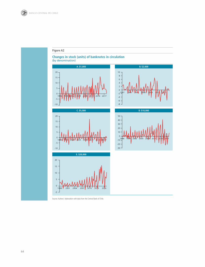
Changes in the stock of banknotes and coins present a high degree of seasonality (figure 5). This is also true for nominal consumption, but the seasonal variations in the two series present some differences. With respect to cash in circulation, it increases sharply the fourth quarter each year (Christmas and New Year effects), and this is followed by a drop in the first quarter the next year. The second and third quarters present only smaller changes. In a simple exercise where the circulating stock is regressed on seasonal dummies, the results indicate than almost 74% of the total variation can be explained by these dummies by means of the R2. As shown in figures A1 and A2 in appendix A, the denominations of the banknotes also present seasonality, while it is less pronounced for the coins.

3. Unit roots

A battery of unit root tests are conducted for the total cash stock in circulation as well as the GDP and the consumption time series, the CPI and the interest rate. The results of the test are reported in table 1, which also presents the estimated coefficient in a simple AR(1) model and its standard error. For the series of durable consumption the tests generally suggest that the series are integrated of order one, I(1), when applying a 5% confidence level. Especially, the stock in circulation seems to be non-stationary, while the results are mixed for the denominations, as shown in table A1 in appendix A. To conclude, the evidence from the unit root tests generally suggests that the variables are non-stationary, even though there are some doubts for some of the denominations.

Table 1

Unit root tests*

TotalStock GDP

Total Cons.

Priv.Cons.

Dur. Cons.

Non dur. Cons.

Serv. Cons. CPI

Interest rate

Coef. AR(1) 0.59 0.72 0.41 0.53 0.46 0.42 0.43 0.87 0.81

(0.09) (0.08) (0.10) (0.09) (0.10) (0.10) (0.10) (0.05) (0.06)

Autoregressive tests

ADF -2.13 -1.77 -2.79 -3.04 -3.82** -2.71 -1.93 -3.09 -2.96

PP (Za) -4.83*** -4.16*** -5.53*** -5.26*** -5.85*** -6.21*** -5.58*** -3.13 -2.88

Efficient tests

ERS Point-optimal 9.72 10.74 5.16** 3.06*** 1.32*** 33.44 12.89 11.57 6.40*

Df-GLS -1.69 -1.72 -2.34 -2.46* -2.91 -1.09 -2.32 -2.21 -2.93*

Ng-Perron (MZa) -10.01 -7.51 -20.85** -27.48*** -46.81*** -2.31 -8.51 -10.30 -14.34*

Stationary test

KPSS 0.21** 0.16** 0.19** 0.17** 0.14* 0.24*** 0.14* 0.06 0.21**

Source: Authors’ elaboration.

(*) Numbers in parentheses are standard errors. The tests and the AR(1) models include a deterministic trend and an intercept. */**/***: Rejection of the null when applying a confidence level of 10%/5%/1%. ADF: Augmented Dickey and Fuller (1979). PP: Phillips and Perron (1988). The critical values applied for ADF and PP are those simulated by MacKinnon (1996). ERS Point-optimal and DF-GLS: Elliott et al. (1996). KPSS: Kwiatkowski et al. (1992). The bandwidths applied for the kernel-based estimations used in PP and KPPS are selected automatically as described in Newey and West (1994). Lag lengths in the other tests are selected according to Schwarz information criterion. The null hypothesis of the KPSS test is stationarity, while it is non-stationarity in the other ones. Bold numbers indicate that the test suggests non-stationarity.

49


IV. FORECASTING TOTAL CASH IN CIRCULATION

This section presents the results of the forecast exercises for the total cash in circulation. Subsection IV.1 presents the econometric models applied, i.e. the cointegrated vector autoregressive (CVAR) models, which include one of the activity variables in nominal terms, the CPI and the interest rate, and the time series models. Then combination of forecasts is discussed. Subsection IV.2 reports the results and contains a brief discussion on the importance of having precise projections of the fundamental variables. To save space, only the results of the best performing models are reported, but all results and tests are available upon request. However, since all the data employed are publically available all results are easy to replicate. The logarithm of the time series is applied before estimation.

1. Econometric models and combinations

Firstly, the cointegrated VAR models are presented followed by the introduction of the time series models. Finally the sub-combinations, which are employed in the forecast exercises, are reported in subsection IV.1.

The cointegrated VAR models

A total of six models are estimated and forecasted, one for each of the activity variables in nominal terms:12 total consumption, private consumption, durable and non-durable consumption, services consumption and GDP. The starting point of the econometric analysis is an unrestricted VAR model,13 which is estimated with five lags14 and includes centered seasonal and temporary dummies,15 besides a deterministic trend and an intercept. With a 5% significance level the Trace test of Johansen (1988, 1995) indicates that each model has at least one cointegrating relation, which is imposed on all systems.16

12 For robustness, three variable models in real terms (real (CPI deflated) outstanding stock, real activity, and nominal short-term rate) were also estimated. Real term specifications rely on a strong assumption of homogeneity with respect to a particular price measure, which may be too restrictive in the case of cash demand (see also Nachane et al. (2013) and Dunbar (2014)). Besides, it would be necessary to have auxiliary CPI projections to obtain forecasts of the nominal outstanding stock. In any case, the root mean square error distances to actual stock observations are smaller for the nominal models in most cases.

13 The econometric model is outlined in appendix B. The VAR model was chosen to allow for endogeneity between the cash demand and the macroeconomic variables included in the analysis.

14 Schwarz information criterion suggests one lag in the unrestricted VAR models, while the Akaike criterion suggests eight lags. The VAR models are estimated with five lags (four in the VECM), which was sufficient, together with the inclusion of some temporary dummies, to obtained errors which are not affected by serial correlation of order one and four according to the Lagrange Multiplier tests and that are no skewed according to the Doornik and Hansen (2008) omnibus test. Juselius (2006) notes that VAR estimates are more sensitive to non-normality due to skewness than to excess kurtosis.

15 The dummies are centered to avoid effects on the underlying asymptotic distribution of the models (see Johansen (1995) and Juselius (2006)). All models include dummies for the third quarter 1998 and the fourth quarter of 1999, where, respectively, the $20000 bill was introduced and there was an extraordinary precautionary demand for cash because of Y2K. Besides that, the models include one and two activity-related dummies.

16 Critical values are from MacKinnon et al. (1999). The model with durable consumption is a borderline case with a p-value of 0.0537 and test for the model with services consumption indicates two cointegrating relations. In this latter case, however, it is not obvious that both of the relations are indeed stationary.

50


Preliminary tests reveal that some of the models make better forecasts when including holiday effect of the Bell and Hillmer (1983) type, while others do not.17 Hence, the models are estimated with and without an exogenous Bell-Hillmer (BH) variable, which leave us with a total of 12 CVAR models.

The time series models

The time series models employed are shown in table 2. They are chosen to take into account the seasonality present in the outstanding cash. The two first ones (Mod 1 and 2) are simple random walk types of models, where the projections are simply the same growth rate as one year ago and the average of the last five years, respectively. Mod 3 is an autoregressive (AR) model of order four and Mod 4 includes seasonal dummies. Mod 5 to 10 are different specifications of SARIMA models.18 The models 3 to 10 are estimated with and without BH effects, such that forecasts are made with a total of 18 time-series models.

Table 2

Time series models*

Name Model Const. BH

Mod 1

Mod 2

Mod 3 Yes Yes

Mod 4 Yes Yes

Mod 5 SARIMA(0,1,1)×(0,0,0)4 Yes Yes







(*) Const: The model includes an intercept. BH: The model is estimated with and without Bell-Hillmer effects.

17 Bell-Hillmer regressors is a simple way to model effects of moving holidays. They assume that there is an interval of days over which the effect of the holiday can be regarded as being the same for each day. In the present context, the Bell-Hillmer coefficient for each quarter is calculated in terms of working days, i.e. holidays over total working days, as this produced better results than number of holidays over total number of days.

18 The models were estimated in Eviews, which should be taking into account if trying to replicate the results of the SARIMA models (see Newbold et al. (1994)).

51


Combining forecasts

One reason for having a system of models for forecasting is that the diversity of the forecasts can be utilized as a measure of uncertainty. Another is that one can combine the predictions,19 which the literature has argued is a good idea since it can be difficult to find a single best model that makes the best forecast as the performance of different models is most likely state-dependent. Hence, there are diversification gains in combining the forecasts from a number of models. Generally, it is recommendable to combine forecasts when (i) the individual forecasts are misspecified, (ii) the forecasting environment is unstable and / or (iii) there is a short track record. The first condition is most likely fulfilled for the forecasts of cash in circulation, as the period of observations is limited, which implies that (iii) is also met. With respect to (ii), as mentioned by Miller (2017), it is particularly difficult to predict cash demand with historical observations as the time series are affected by possible structural breaks due to factors such as changes of the denominations employed in the economy, the development of the informal sector, the way consumers make and pay for purchases (for example, the introduction of on-line shopping), etc. Hence, combining forecasts to predict cash demand seems to be suitable, and particularly for the demand for different denominations.

There are several ways that the forecasts can be combined and in the present context we choose the simple average, i.e. assigning the same weight to each of the projections. While there is no theoretical reason for equal weights to be the optimal combination scheme (Diebold and Shin, 2017),20 the empirical literature frequently finds that the simple average performs better than more sophisticated combinations (Smith and Wallis, 2009). This has been named the Forecast Combination Puzzle by Stock and Watson (2004). To limit the effects of extreme projections, we also calculate the median forecast.

Beside the average and median forecasts of all the models (VAR and time series models with and without BH effects), the same measures are calculated for some sub-combinations in order to evaluate how well they perform compared to the overall average / median. The following sub-combinations are evaluated: • VAR models: with BH effects, without BH effects and all forecasts included.• Time series models: with BH effects, without BH effects and all forecasts

included.• VAR and time series models: with BH effects and without BH effects.

2. Forecasting

The forecast exercise consists in estimating the models with observations until 2008Q4, i.e. twelve years when including four lags, and make forecasts up till

19 For a recent overview of forecast combinations, see Elliott and Timmermann (2016).

20 Diebold and Shin (2017) do argue, however, that simple averages are likely to be nearly optimal even if not fully optimal.

52


three years ahead. Then a year of observations is added to the estimation sample and the exercise is repeated until forecasts are available to 2017Q4.21 This leaves us with a total of nine one-year-ahead forecasts, eight two years ahead and seven three years ahead. Thus, the number of predictions is very limited, which has to be taken into account when reading the results. As is standard in the literature, the results are reported by the root mean squared error (RMSE22), which is normalized with the average forecast of all the models such that values higher (lower) than one indicate the forecasts are worse (better) than the average. The results for the median as well as the best of the sub-combinations and individual models, reported in table C1 in appendix C, are shown in figure 6.

Figure 6

Total circulation: Relative RMSE of out-of-sample forecasts*

0.0

0.2

0.4

0.6

0.8

1.0

1.2

Median Best combination Best individual


(*) RMSE of forecasts with respect to the average forecast. The bars represent predictions one, two, and three-years-ahead, respectively. Dotted bars (of which there are none in figure 6) indicate that the difference of the mean squared errors are statistically different according to the Diebold and Mariano (1995) test with the Harvey et al. (1997) small-sample correction.

Table 3

Forecast statistics. Total stock in circulation*

1-year-ahead 2-years-ahead 3-years-ahead

Better Under. (3/9) Better Under. (4/8) Better Under. (4/7)

Median 3/9 3/9 3/8 4/8 3/7 4/7

Sub-comb. 4/9 3/9 3/8 3/8 3/7 3/7

Individual 3/9 3/9 4/8 3/8 3/7 3/7

Source: Authors’ elaboration. (*) Better: Relative number of times the absolute error is less than that of the average. Under: Relative number of underestimations. The numbers in parenthesis is for the average.

21 The out-of-sample forecast exercise is pseudo in the sense that the models are estimated with the most recent vintage, 1996Q1 – 2017Q4 of the activity variable, which includes revisions that are not available in real time. Furthermore, tests for cointegration and misspecification are performed with the full sample.

22 , where E(yt) is the forecast of the variable yt and n is the number of available forecasts.

53


While it is possible to find sub-combinations and individual models that perform better than the average, the gains are quite limited and not statistically significantly.23 Due to the very limited number of forecasts, some additional statistics are presented in table 3. It turns out that none of the forecasts is better than the average more than half of the times and the average forecast is not more biased than the others. Hence, in the context of the models evaluated in the present paper, it is concluded that the average forecast is quite good.

The impact of accurate forecasts of the fundamental variables

As an experiment, this subsection analyzes the extent to which better forecasts could be obtained with perfect foresight of the fundamental variables. This serves to evaluate whether it is recommendable to include exogenously made forecasts of these variables instead of utilizing the dynamic forecasts of the VAR models. It cannot be stressed enough that this is merely an experiment and no discussion is included of, for example, the increased forecast uncertainty. The models are simple regressions, which include the change in the (nominal) total cash on the left-hand-side of the equality and the contemporaneous values of the activity variable, the CPI and the interest rate on the right-hand-side as well as a constant term and some outlier dummies. The regressions are estimated recursively and forecasts are made out-of-sample, but with the actual values of the fundamental variables. Figure 7 shows the relative RMSE of the average perfect foresight forecast and the average applied in figure 6. It is not evident that precise predictions of the fundamental variables improve the forecasts of the two shortest horizons, but there seems to be some gain at the longest one. Hence, good forecasts of economic activity, price development and the interest rate seem to be valuable input for the estimation of the future (long-run) circulation of cash.

Figure 7

Effects of accurate predictions of fundamental variablesRelative RMSE of out-of-sample forecasts*

0.0

0.2

0.4

0.6

0.8

1.0

1.2

1.4

1.6


(*) See figure 6. The average forecast used for comparison is the same as in figure 6.

23 The test applied is that of Diebold and Mariano (1995) with the small sample correction proposed by Harvey et al. (1997), see appendix D. It should be emphasized, however, that the outcomes are merely indicative as a very small sample of forecasts is available.

54


V. FORECASTING DENOMINATIONS OF BANKNOTES AND COINS

The models applied in this section are the same as the ones presented in the previous one, but the variables forecasted are number of units that circulate of each coin and banknote denomination. Furthermore, CVAR models are also estimated with real variables and, for comparison, the results are also contrasted with those of CPV.24 The results are reported in subsection V.1, while subsection V.2 discusses whether forecasts of the total cash stock in circulation should be made with aggregated forecasts or the aggregation of disaggregated ones.

1. Forecast exercises

The results of the forecast exercises are shown in figure 8 for the coins and in figure 9 for the banknotes. Often the RMSE are smaller for the median, the best sub-combination or an individual model, and many times the differences are statistically significant. Particularly, the median does often perform slightly better than the average. The individual models that perform best are frequently time series, which is to be expected as there are no theoretical arguments for fundamental variables to explain variations in the denominations of coins and banknotes.

Figure 8

Coins: Relative RMSE of out-of-sample forecasts*

A. $10 B. $50

0.0

0.5

1.0

1.5

2.0

2.5

3.0

Median Bestcombination

Bestindividual

CPV Median Bestcombination

Bestindividual

CPV0.0

0.5

1.0

1.5

2.0

2.5

3.0

3.5

C. $100 D. $500


Bestindividual

CPV0.0

0.2

0.4

0.6

0.8

1.0

1.2

1.4

1.6

1.8


Bestindividual

CPV0.0

0.2

0.4

0.6

0.8

1.0

1.2

1.4


(*) See figure 6. CPV are the forecasts made with the model of Chumacero et al. (2008). The average forecast is that of all the models per denomination.

24 These forecasts are made with the program elaborated by Rómulo Chumacero for the CBCh.

55


Figure 9

Banknotes: Relative RMSE of out-of-sample forecasts*

A. $1,000 B. $2,000


Bestindividual

CPV0.0

0.2

0.4

0.6

0.8

1.0

1.2


Bestindividual

CPV0.0

0.2

0.4

0.6

0.8

1.0

1.2

1.4

C. $5,000 D. $10,000


Bestindividual

CPV0.0

0.2

0.4

0.6

0.8

1.0

1.2


Bestindividual

CPV0.0

0.2

0.4

0.6

0.8

1.0

1.2

1.4

E. $20,000


Bestindividual

CPV0.0

0.2

0.4

0.6

0.8

1.0

1.2


(*) See figure 8.

Turning to the statistics of the forecasts, which are reported in tables 4 and 5, they generally confirm the evidence from the figures. It is noteworthy that the median often makes better coin projections than the average, while it is not clear that this is true for the banknotes. More often than not, however, some sub-combination or individual models beat the average (and the median) when forecasting denominations. Again, it should be remembered that this evaluation is made with few observations and more predictions are probably necessary for taking advantage of the benefits of combining the forecasts.

56


Table 4

Forecast statistics. Coins*


Better Neg. Better Neg. Better Neg.

$10 (4/9) (3/8) (3/7)

Median 8/9 4/9 8/8 3/8 6/7 3/7

Sub-comb. 7/9 4/9 6/8 3/8 6/7 3/7

Individual 7/9 4/9 6/8 2/8 4/7 3/7

CPV 3/9 3/9 3/8 3/8 2/7 3/7

$50 (4/9) (2/8) (1/7)

Median 6/9 4/9 7/8 3/8 4/7 0/7

Sub-comb. 5/9 2/9 7/8 2/8 3/7 2/7

Individual 2/9 5/9 4/8 3/8 2/7 2/7

CPV 3/9 6/9 1/8 6/8 2/7 7/7

$100 (2/9) (2/8) (1/7)

Median 8/9 2/9 6/8 2/8 6/7 1/7

Sub-comb. 8/9 2/9 7/8 2/8 6/7 1/7

Individual 6/9 5/9 7/8 2/8 5/7 2/7

CPV 4/9 3/9 3/8 2/8 4/7 3/7

$500 (2/9) (1/8) (0/7)

Median 6/9 4/9 7/8 4/8 6/7 4/7

Sub-comb. 6/9 3/9 8/8 3/8 7/7 3/7

Individual 6/9 3/9 8/8 4/8 7/7 4/7

CPV 4/9 5/9 6/8 7/8 5/7 7/7


(*) See table 3. CPV is the model of Chumacero et al. (2008).

57


Table 5

Forecast statistics – Banknotes*


Better Neg. Better Neg. Better Neg.

$1000 (7/9) (7/8) (7/7)

Median 3/9 7/9 4/8 7/8 4/7 7/7

Sub-comb. 6/9 7/9 6/8 7/8 6/7 7/7

Individual 6/9 5/9 7/8 5/8 7/7 5/7

CPV 5/9 7/9 5/8 8/8 4/7 7/7

$2000 (3/9) (1/8) (1/7)

Median 5/9 3/9 6/8 1/8 3/7 1/7

Sub-comb. 7/9 4/9 6/8 3/8 6/7 1/7

Individual 8/9 4/9 5/8 3/8 6/7 3/7

CPV 3/9 2/9 2/8 1/8 2/7 0/7

$5000 (2/9) (2/8) (2/7)

Median 4/9 2/9 4/8 2/8 4/7 2/7

Sub-comb. 7/9 5/9 7/8 2/8 6/7 3/7

Individual 6/9 5/9 7/8 2/8 4/7 3/7

CPV 5/9 3/9 7/8 2/8 5/7 2/7

$10000 (4/9) (4/8) (4/7)

Median 4/9 3/9 4/8 4/8 5/7 4/7

Sub-comb. 5/9 3/9 4/8 3/8 6/7 4/7

Individual 6/9 3/9 5/8 2/8 5/7 4/7

CPV 3/9 2/9 2/8 2/8 2/7 0/7

$20000 (2/9) (3/8) (2/7)

Median 5/9 3/9 4/8 4/8 3/7 6/7

Sub-comb. 5/9 2/9 5/8 6/8 7/7 2/7

Individual 5/9 3/9 4/8 4/8 3/7 3/7

CPV 6/9 3/9 4/8 5/8 3/7 6/7


(*) See table 4. CPV is the model of Chumacero et al. (2008).

2. Aggregate or disaggregate forecasts?

As a final experiment, we analyze if the aggregation of the individual denomination forecasts makes better forecasts of the total stock of cash in circulation compared to the average aggregate forecasts.25 The results, shown in figure 10, indicate that this is not the case. For all horizons, the aggregated predictions are better than the sum of the disaggregated ones. Hence, the evidence from this experiment suggests that one can obtain better predictions of the total circulating stock by making aggregate forecasts.

25 There is a huge literature on aggregation versus disaggregation in forecasting. As mentioned by Hendry and Hubrich (2011), from a theoretically point of view (see references in the Hendry and Hubrich article) aggregating component forecasts will generally be at least as accurate as directly forecasting the aggregate when the data generating process (DGP) is known. In practice, however, the DGP is not known and, hence, it is mainly an empirical question whether aggregating component predictions improves the accuracy compared with the aggregate forecast.

58


Figure 10

Forecasting the aggregate cash in circulation or by denominations?Relative RMSE of out-of-sample forecasts*

0.0

0.2

0.4

0.6

0.8

1.0

1.2

1.4

1.6


(*) See figure 6. The average forecast used for comparison is that of the aggregate forecast.

VI. CONCLUDING REMARKS

In planning the purchases and future delivery of Chilean cash, it is crucial to have forecasts of the future demand as reliable as possible. It is, however, important to emphasize that in Chile, approximately 75% of new banknotes are put into circulation to replace pieces that are no longer suitable, such that knowledge of the expected duration of the notes is vital for the stock management, an issue that is beyond the scope of the present analysis.

Changes in the stock in circulation is the other main component and we proposed a system of models that can be used to forecast the total circulating stock of coins and banknotes as well as each of the denominations. In this context we advocated for combing the forecasts of the individual models. With the very limited data available to evaluate the annual forecasts, the evidence suggested that the simple average of the forecasts is quite good for forecasting the total outstanding stock. The evidence for the denominations was not as favorable because often sub-combinations or individual models had better forecast performances. It was argued, however, that it might still be a good idea to combine the forecasts as the evaluations are made with few observations. As more data become available, future evidence will reveal the extent to which the combination improves its performance.

The quest to find suitable models for forecasting never ends. Structural shifts and other changes of conditions may require updating the existing models or even changing them for new ones. Usually it is advisable to have different models with different kinds of focus such that the input, not only of the actual forecasts, but also of past errors, can be used in the judgment of making the final purchase decisions. In the present paper we argued for combining several

59


forecasts and presented a system with time series models as well as some based on fundamental macroeconomic variables. Another direction would be to explore models in line with those utilized by Gerst and Wilson (2011) and Vale (2015), which take into account technology development and consumer taste, or that of Miller (2017) that tried out several macroeconomic variables that may affect the use of cash. To what extent these characteristics can be employed formally in econometric models depends on the availability of data, and the development of such a framework is left to future research.

60


REFERENCES

Akinci, Ö. (2003). “Modelling the Demand for Currency Issued in Turkey.” Central Bank Review 3(1): 1-25.

Amromin, G. and S. Chakravorti (2009). “Whither Loose Change? The Diminishing Demand for Small Denomination Currency.” Journal of Money, Credit and Banking 41(2-3): 315–35.

Bagnall, J., D. Bounie, K.P. Huynh, A. Kosse, T. Schmidt, S. Schuh, and H. Stix (2014). “Consumer Cash Usage. A Cross-country Comparison with Payment Diary Survey Data.” Working Paper No. 1685, European Central Bank.

Barnett, W., D. Fisher, and A. Serletis (1992). “Consumer Theory and the Demand for Money.” Journal of Economic Literature 30(4): 2086–119.

Bartzsch, N., F. Seitz, and R. Setzer (2015). “The Demand for Euro Banknotes in Germany: Structural Modelling and Forecasting.” MPRA paper 64949, University Library of Munich, Germany.

Baumol, W.J. (1952). “The Transactions Demand for Cash: An Inventory Theoretic Approach.” Quarterly Journal of Economics 66(4): 545–56.

Bell, W.R. and S.C. Hillmer (1983). “Modelling Time Series with Calendar Variation.” Journal of the American Statistical Association 78(383): 526–34.

Briglevics, T. and S. Schuh (2014). “U.S. Consumer Demand for Cash in the Era of Low Interest Rates and Electronic Payments.” Working Paper No. 1660, European Central Bank.

Central Bank of Chile (2016): Financial Stability Report, first half.

Chumacero, R.A., C. Pardo, and D. Valdés (2008). “Un Marco para la Elaboración de los Programas de Impresión y Acuñación.” Economía Chilena 11(1): 29–59.

Columba, F. (2009). “Narrow Money and Transaction Technology: New Disaggregated Evidence.” Journal of Economics and Business 61(4): 312–25.

Cusbert, T. and T. Rohling (2013). “Currency Demand during the Global Financial Crisis: Evidence from Australia.” Research Discussion Paper 2013-01, Reserve Bank of Australia.

Dickey, D.A. and W.A. Fuller (1979). “Distribution of the Estimators for Autoregressive Time Series with a Unit Root.” Journal of the American Statistical Association 74(366): 427–31.

Diebold, F.X. and R. Mariano (1995). “Comparing Predictive Accuracy.” Journal of Business and Economic Statistics 13(3): 253–65.

61


Diebold, F.X. and M. Shin (2017). “Beating the Simple Average: Egalitarian LASSO for Combining Economic Forecasts.” PIER Working Paper No. 17-017. Available at SSRN: https://ssrn.com/abstract=3032492 or http://dx.doi.org/10.2139/ssrn.3032492.

Doornik, J. and H. Hansen (2008). “An Omnibus Test for Univariate and Multivariate Normality.” Oxford Bulletin of Economics and Statistics 70(Supplement s1): 927–39.

Doyle, B.M. (2000). “‘Here, Dollars, Dollars…’ – Estimating Currency Demand and Worldwide Currency Substitution.” International Finance Discussion Paper No. 330, Board of Governors of the Federal Reserve System.

Duca, J.V. and D.D. VanHoose (2004). “Recent Developments in Understanding the Demand for Money.” Journal of Economics and Business 56(4): 247–72.

Dunbar, G.R. (2014). “Demographics and the Demand for Currency.” Working Paper 2014-59, Bank of Canada.

Elliott, G., T.J. Rothenberg and J. Stock (1996). “Efficient Test for an Autoregressive Unit Root.” Econometrica 64(4): 813–36.

Elliott, G. and A. Timmermann (2016): Economic Forecasting, Princeton University Press.

Fischer, B., P. Köhler, and F. Seitz (2004). “The Demand for Euro Area Currencies: Past, Present and Future.” Working Paper 330, European Central Bank.

Gerst, J. and D.J. Wilson (2011). “An Analytical Framework for the Forecasting and Risk Assessment of Demand for Fed Cash Services.” Technical Paper, Federal Reserve Bank of San Francisco.

Harvey, D.I., S.J. Leybourne, and P. Newbold (1997). “Testing the Equality of Prediction Mean Squared Errors.” International Journal of Forecasting 13(2): 281–91.

Hendry, D.F. and K. Hubrich (2011). “Combining Disaggregate Forecasts or Combining Disaggregate Information to Forecast an Aggregate.” Journal of Business and Economic Statistics 29(2): 216–27.

Johansen, S. (1988). “Statistical Analysis of Cointegration Vectors.” Journal of Economic Dynamic and Control 12(2–3): 231–54.

Johansen, S. (1995): Likelihood-Based Inference in Cointegrated Vector Autoregressive Models, Second print, Oxford University Press.

Juselius, K. (2006). The Cointegrated VAR Model: Methodology and Applications, Oxford University Press.

Khamis, M. and A. Leone (2001). “Can Currency Demand Be Stable under a Financial Crisis? The Case of Mexico.” IMF Staff Papers 48, 344-366.

62


Kwiatkowski, D., P. Phillips, P. Schmidt, and Y. Shin (1992). “Testing the Null Hypothesis of Stationarity against the Alternative of a Unit Root: How Sure Are We that Economic Time Series Have a Unit Root?” Journal of Econometrics 54(1–3): 159–78.

MacKinnon, J.G. (1996). “Numerical Distribution Functions for Unit Root and Cointegration Tests.” Journal of Applied Econometrics 11(6): 601–18.

MacKinnon, J.G., A.A. Haug, and L. Michelis (1999). “Numerical Distribution Functions of Likelihood Ratio Tests for Cointegration.” Journal of Applied Econometrics 14(5): 563–77.

Miller, C. (2017). “Addressing the Limitations of Forecasting Banknote Demand.” International Cash Conference 2017 – War on Cash: Is there a Future for Cash? 25–27 April, Island of Mainau, Germany.

Nachane, D.M., A.B. Chakraborty, A.K. Mitra, and S. Bordoloi (2013). “Modelling Currency Demand in India: An Empirical Study.” Study No. 39, Department of Economic and Policy Research, Reserve Bank of India.

Newbold, P., C. Agiakloglou, and J. Miller (1994). “Adventures with ARIMA Software.” International Journal of Forecasting 10(4): 573–81.

Newey, W.K. and K.D. West (1994). “Automatic Lag Selection in Covariance Matrix Estimation.” Review of Economic Studies 61: 631–53.

Phillips, P.C.B. and P. Perron (1988). “Testing for a Unit Root in Time Series Regression.” Biometrika 75(2): 335–46.

Sastry, A.S.R. (1970). “The Effect of Credit on Transactions Demand for Cash.” Journal of Finance 25(4): 777–81.

Smith, J. and K.F. Wallis (2009). “A Simple Explanation of the Forecast Combination Puzzle.” Oxford Bulleting of Economics and Statistics 71(3): 331–55.

Stock, J.H. and M.W. Watson (2004). “Combination Forecasts of Output Growth in a Seven-Country Data Set.” Journal of Forecasting 23(6): 405–30.

Tobin, J. (1956). “The Interest Elasticity of the Transactions Demand for Cash.” Review of Economics and Statistics 38(3): 241–47.

Vale, B. (2015). “Forecasting Demand for Various Denominations of Notes and Coins Using Error Correction Models.” Staff Memo No. 1, Norges Bank.

63


APPENDIX A

SUPPLEMENTARY MATERIAL TO SECTION III

Figure A1

Changes in stock (units) of coins in circulation(by denomination)

A. $10 B.$50

0

20

40

60

80

100

120

140

160

1996 1999 2002 2005 2008 2011 2014 2017 19991996 2002 2005 2008 2011 2014 2017-2

0

2

4

6

8

10

12

14

16

C. $100 D. $500

19991996 2002 2005 2008 2011 2014 2017-505

101520253035404550

2000 2003 2006 2009 2012 2015

-5

0

5

10

15

20


64


Figure A2

Changes in stock (units) of banknotes in circulation(by denomination)

A. $1,000 B. $2,000

19991996 2002 2005 2008 2011 2014 2017

-10

-5

0

5

10

15

20

20001997 2003 2006 2009 2012 2015

-8

-6

-4

-2

0

2

4

6

8

10

C. $5,000 D. $10,000

19991996 2002 2005 2008 2011 2014 2017

-10

-5

0

5

10

15

20

19991996 2002 2005 2008 2011 2014 2017

-30

-20

-10

0

10

20

30

40

50

E. $20,000

1998 2001 2004 2007 2010 2013 2016

-5

0

5

10

15

20


65


Table A1

Unit root tests*

$10 $50 $100 $500 $1,000 $2,000 $5,000 $10,000 $20,000

Coeff. AR(1) 0.99 0.92 0.98 0.60 0.95 0.86 0.89 0.84 0.39

(0.02) (0.04) (0.02) (0.02) (0.03) (0.03) (0.05) (0.06) (0.05)

Autoregressive tests

ADF -3.51** -2.39 -3.91** -6.00*** -1.31 -2.25 -3.27* -2.53 -1.76

PP (Za) -1.08 -2.32 -1.19 -19.49*** -1.08 -4.35*** -2.18 -2.84 -13.52***

Efficient tests

ERS Point-optimal 10.30 8.06 4.25** 1566.09 323.43 331.11 3.08*** 0.03*** 1708.08

Df-GLS -3.15** -2.22 -3.13** 0.47 -1.54 -0.28 -2.93* -2.43 -4.59***

Ng-Perron (MZa) -31.64*** -12.13 -59.85*** -2.69 -22.43** -0.20 -148.79*** -2119.92*** 0.15

Stationary test

KPSS 0.27*** 0.07 0.22*** 0.16** 0.29*** 0.28*** 0.15** 0.16** 0.10


(*) Numbers in parentheses are standard errors. The tests and the AR(1) models include a deterministic trend and an intercept. */**/***: Rejection of the null when applying a confidence level of 10%/5%/1%. ADF: Augmented Dickey and Fuller (1979). PP: Phillips and Perron (1988). The critical values applied for ADF and PP are those simulated by MacKinnon (1996). ERS Point-optimal and DF-GLS: Elliott et al. (1996). KPSS: Kwiatkowski et al. (1992). The bandwidths applied for the kernel-based estimations used in PP and KPPS are selected automatically as described in Newey and West (1994). Lag lengths in the other tests are selected according to Schwarz information criterion. The null hypothesis of the KPSS test is stationarity, while it is non-stationarity in the other ones. Bold numbers indicate that the test suggests non-stationarity.

66


APPENDIX B

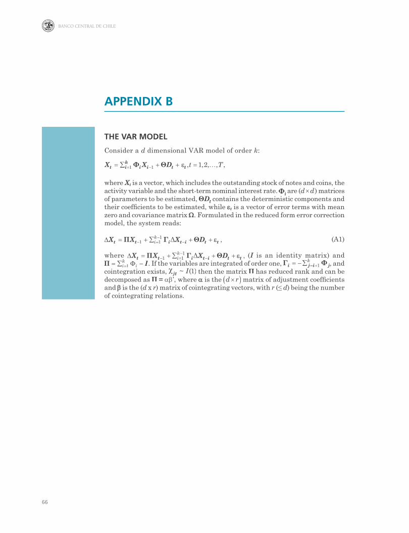
THE VAR MODEL

Consider a d dimensional VAR model of order k:

where Xt is a vector, which includes the outstanding stock of notes and coins, the activity variable and the short-term nominal interest rate. are (d d) matrices of parameters to be estimated, contains the deterministic components and their coefficients to be estimated, while et is a vector of error terms with mean zero and covariance matrix W. Formulated in the reduced form error correction model, the system reads:

(A1)

where (I is an identity matrix) and . If the variables are integrated of order one, , and

cointegration exists, then the matrix has reduced rank and can be decomposed as = ab’, where a is the matrix of adjustment coefficients and b is the (d x r) matrix of cointegrating vectors, with r (≤ d) being the number of cointegrating relations.

67


APPENDIX C

MODELS WITH THE BETTER FORECAST PERFORMANCES

Table C1

Best sub-combinations and individual models*

Sub-combination Individual model

1Y 2Y 3Y 1Y 2Y 3Y

Stock M Comb A VAR A TS w/BH M9 w /BH Tot Serv w/BH

Coins

$10 M Comb A VAR w/BH A VAR w/BH M4 M5 w/BH M5 w/BH

$50 M VAR w/BH M VAR w/BH M VAR Priv Non-dur w/BH Dur

$100 M ST A ST w/BH M ST M4 M4 M4

$500 M All-R M All-R M All-R M2 M2 M2

Banknotes

$1000 M TS w/BH M VAR M VAR w/BH M2 M3 M4

$2000 A VAR A VAR w/BH A VAR Priv Priv w/BH Priv

$5000 A TS w/BH A TS w/BH M TS w/BH M1 M1 M3 w/BH

$10000 A TS w/BH A VAR A TS w/BH M1 M1 M7

$20000 A Comb A VAR A Comb M4 M8 w/BH m8 w/BH


(*) A: Average. M: Median. VAR: VAR models. TS: Time series models. Comb: VAR and time series models (nominal terms). All-R: All models excluding those with real variables. w/BH: Model includes BH effects. Mi: Time series model Mod i (i=1,2,…,10). Cons / Serv / Priv / Non-dur / Dur: VAR model where the activity variable is total / services / private / non-durable / durable consumption.

68


APPENDIX D

THE SMALL SAMPLE CORRECTED DIEBOLD-MARIANO TEST

The applied test of Diebold and Mariano (1995) is based on the squared forecast error;

where E(yit) is the forecast of variable yt made by model i. The null hypothesis of the test is that the expected difference of the forecast errors is zero:

while the alternative is that it is different from zero. Letting be the average difference, n the number of forecasts, and V(dt) the long-run

(HAC) covariance of the differences, the test statistic is:

which has a standard Gaussian distribution. If h denotes the forecast horizon, the small sample corrected test statistic proposed by Harvey et al. (1997) reads:

which has a t distribution with n–1 degrees of freedom.

a system for forecasting chilean cash demand–the …

Documents