a portable bioimpedance spectroscopy system for congestive
TRANSCRIPT

A Portable Bioimpedance Spectroscopy System forCongestive Heart Failure Management
by
Maggie Delano
B.S., Massachusetts Institute of Technology (2010)M.Eng., Massachusetts Institute of Technology (2012)
Submitted to the Department of Electrical Engineering and ComputerScience
in partial fulfillment of the requirements for the degree of
Doctor of Philosophy
at the
MASSACHUSETTS INSTITUTE OF TECHNOLOGY
February 2018
c Massachusetts Institute of Technology 2018. All rights reserved.
Author . . . . . . . . . . . . . . . . . . . . . . . . . . . . . . . . . . . . . . . . . . . . . . . . . . . . . . . . . . . . . . . .Department of Electrical Engineering and Computer Science
January 3, 2018
Certified by. . . . . . . . . . . . . . . . . . . . . . . . . . . . . . . . . . . . . . . . . . . . . . . . . . . . . . . . . . . .Charles G. Sodini
LeBel Professor of Electrical EngineeringThesis Supervisor
Accepted by . . . . . . . . . . . . . . . . . . . . . . . . . . . . . . . . . . . . . . . . . . . . . . . . . . . . . . . . . . .Leslie A. Kolodziejski
Professor of Electrical Engineering and Computer ScienceChair, Department Committee on Graduate Students

2

A Portable Bioimpedance Spectroscopy System for Congestive
Heart Failure Management
by
Maggie Delano
Submitted to the Department of Electrical Engineering and Computer Scienceon January 3, 2018, in partial fulfillment of the
requirements for the degree ofDoctor of Philosophy
Abstract
Congestive Heart Failure (CHF) is a chronic medical condition that causes reducedexercise tolerance, shortness of breath, and fluid buildup in the lungs, legs, and ab-domen. While CHF-related mortality has reduced in recent years, this reduction hasbeen accompanied by an increase in hospitalizations and readmissions. This thesistakes the first steps toward developing a compression sock based bioimpedance mon-itoring system for patients with CHF to help reduce readmission rates. The primarygoals of the thesis were to better understand the calf bioimpedance measurement ina controlled environment (hemodialysis) and to develop portable hardware to per-form measurements. Calf bioimpedance was measured on 17 patients undergoinghemodialysis using both a commercial measurement system and the experimentalsystem developed in this thesis. Measured calf bioimpedance data showed that morefluid is recruited from the calf at higher ultrafiltration rates. Fluid shifts into or out ofcells also depended on the ultrafiltration rate. It was also observed that patients withhigh calf fluid overload accumulate fluid in the calf, rather than lose it. Bioimpedancemeasurements were also compared between the side of the leg and back of the leg.Changes in calf bioimpedance were higher on the back in 4/7 patients measured, sug-gesting that ideal electrode placement depends on the individual patient. Finally, aportable bioimpedance system was developed and verified against a commercial sys-tem on the bench and during hemodialysis. The two systems measured bioimpedancechanges within 2 Ω in most cases, with outliers limited to patients with particularlylow calf bioimpedance. While the relationship between calf fluid status and total fluidstatus is complex, there is likely utility in calf bioimpedance measurements for CHFremote monitoring. In the ideal use case, patients will start out at dry weight andgain comparable amounts of fluid compared with the fluid removed during hemodial-ysis. This should result in measurable calf bioimpedance changes on the same orderof those measured here. Additionally, rates of both fluid accumulation and removalwill be an order of magnitude slower than hemodialysis, so volume compartmentsshould be in equilibrium, unlike immediately following hemodialysis as was measuredin this thesis.
3

Thesis Supervisor: Charles G. SodiniTitle: LeBel Professor of Electrical Engineering
4

Acknowledgments
I would first like to thank my research supervisor Professor Charlie Sodini. I am
grateful for all I’ve learned from Charlie over the years, from how to interrogate data
to how to present a compelling argument. I’m also thankful for Charlie’s support
for me outside the lab, and his encouragement for self-care and boundaries around
research (“always make time for lunch”). Charlie always paves his own path, a trait I
hope to emulate in my future work.
I would also like to thank the other members of my committee, Profs. Collin
Stultz and Thomas Heldt. I’m particularly thankful for the frequent meetings they
had with me leading up to my thesis defense. They challenged me when I needed to
be challenged, and reassured me when I needed reassurance.
Sodini group members Joohyun Seo, Sidney Primas, Dr. Katherine Smyth and
Dr. Sabino Pietrangelo provided insight and support throughout the research process,
including giving detailed feedback on presentations.
I would like to thank Tom O’Dwyer and Analog Devices for their support of
this research. Tom provided valuable insight that ultimately improved the work in
a number of areas. This project’s funding was made possible by the MIT Medical
Electronic Device Realization Center (MEDRC) and the MIT Center for Integrated
Circuits and Systems (CICS).
I would like to thank everyone who made the clinical testing in this thesis possi-
ble, including those at MGH (Dr. Maulik Majmudar, Dr. Herbert Lin, Haley Dalzell,
Bianca Lavelle, Divya Padmanabhan, and Rachel Lopdrup) and those at MIT (Dr.
Cathy Ricciardi and Tatiana Levkovich). Dr. Majmudar and Dr. Lin provided phys-
iological insights and assistance navigating the approval process for the hemodialysis
studies presented here. Haley, Bianca, Divya, and Rachel conducted patient screening
and consent. Dr. Ricciardi and Tatiana performed consent and assisted with clinical
procedures for the repeatability measurements.
My partner Kendra Albert not only prepared cookies for my thesis defense (a
promise made 3.5 years ago that they may have come to regret), but also supported
5

me during the ups and downs of graduate life. I’m also grateful for my parents, Mark
and Maureen Delano, who supported my interest in science and research from an
early age. I would also like to thank all the friends that I’ve made over my time at
MIT, who not only made my time more fun, but also more meaningful.
6

Contents
List of Figures 13
List of Tables 17
1 Introduction and Motivation 19
1.1 Background . . . . . . . . . . . . . . . . . . . . . . . . . . . . . . . . 19
1.2 CHF Overview . . . . . . . . . . . . . . . . . . . . . . . . . . . . . . 20
1.2.1 Classification . . . . . . . . . . . . . . . . . . . . . . . . . . . 20
1.2.2 Body Composition . . . . . . . . . . . . . . . . . . . . . . . . 21
1.2.3 Pathophysiology of CHF . . . . . . . . . . . . . . . . . . . . . 21
1.2.4 Timeline to CHF Hospitalization . . . . . . . . . . . . . . . . 23
1.3 Remote Fluid Status Monitoring in CHF . . . . . . . . . . . . . . . . 25
1.3.1 Pressure Based Methods . . . . . . . . . . . . . . . . . . . . . 25
1.3.2 Bioimpedance Based Methods . . . . . . . . . . . . . . . . . . 26
1.4 Problem Statement . . . . . . . . . . . . . . . . . . . . . . . . . . . . 27
1.5 Thesis Aims . . . . . . . . . . . . . . . . . . . . . . . . . . . . . . . . 28
1.6 Thesis Organization . . . . . . . . . . . . . . . . . . . . . . . . . . . . 29
2 Bioimpedance 31
2.1 Introduction to Bioimpedance . . . . . . . . . . . . . . . . . . . . . . 31
2.2 Tissue Properties and Modeling . . . . . . . . . . . . . . . . . . . . . 31
2.2.1 Three Element Circuit Model . . . . . . . . . . . . . . . . . . 32
2.2.2 Cole Model . . . . . . . . . . . . . . . . . . . . . . . . . . . . 34
7

2.2.3 The Alpha Term . . . . . . . . . . . . . . . . . . . . . . . . . 35
2.2.4 Stray Capacitance in Bioimpedance Measurements . . . . . . 35
2.3 Estimating Fluid Volume . . . . . . . . . . . . . . . . . . . . . . . . . 36
2.3.1 Bioelectrical Impedance Analysis . . . . . . . . . . . . . . . . 36
2.3.2 Bioimpedance Spectroscopy . . . . . . . . . . . . . . . . . . . 39
2.4 Classifying Patients Based on Bioimpedance Data . . . . . . . . . . . 43
2.4.1 Bioelectrical Impedance Vector Analysis . . . . . . . . . . . . 43
2.4.2 ECW/TBW ratio . . . . . . . . . . . . . . . . . . . . . . . . . 43
2.4.3 Body Composition Monitor . . . . . . . . . . . . . . . . . . . 44
2.4.4 Healthy CNR Range . . . . . . . . . . . . . . . . . . . . . . . 45
2.5 Discussion . . . . . . . . . . . . . . . . . . . . . . . . . . . . . . . . . 47
2.5.1 Distinguish ECW and ICW . . . . . . . . . . . . . . . . . . . 48
2.5.2 Accurately Track ECW Changes . . . . . . . . . . . . . . . . . 49
2.5.3 Hydration Classification . . . . . . . . . . . . . . . . . . . . . 49
2.5.4 Robust Measurement . . . . . . . . . . . . . . . . . . . . . . . 49
2.5.5 Integration into Wearable . . . . . . . . . . . . . . . . . . . . 50
2.5.6 Patient Compliance . . . . . . . . . . . . . . . . . . . . . . . . 50
2.5.7 Measurements in this Thesis . . . . . . . . . . . . . . . . . . . 51
2.6 Chapter Summary . . . . . . . . . . . . . . . . . . . . . . . . . . . . 51
3 Fluid Status Changes in the Calf During Hemodialysis 53
3.1 Introduction to Hemodialysis . . . . . . . . . . . . . . . . . . . . . . 53
3.1.1 The Process of Hemodialysis . . . . . . . . . . . . . . . . . . . 53
3.1.2 At Rest . . . . . . . . . . . . . . . . . . . . . . . . . . . . . . 54
3.1.3 Diffusive Hemodialysis . . . . . . . . . . . . . . . . . . . . . . 56
3.1.4 Ultrafiltration . . . . . . . . . . . . . . . . . . . . . . . . . . . 57
3.1.5 Combined Hemodialysis . . . . . . . . . . . . . . . . . . . . . 59
3.1.6 Calf Bioimpedance Changes During Hemodialysis . . . . . . . 60
3.2 Clinical Testing Methods . . . . . . . . . . . . . . . . . . . . . . . . . 60
3.2.1 Inclusion / Exclusion Criteria . . . . . . . . . . . . . . . . . . 60
8

3.2.2 Study Procedures . . . . . . . . . . . . . . . . . . . . . . . . . 61
3.2.3 Calculating Bioimpedance Parameters . . . . . . . . . . . . . 62
3.2.4 Calculating Calf Volumes . . . . . . . . . . . . . . . . . . . . 64
3.2.5 Evaluation of Fluid Status . . . . . . . . . . . . . . . . . . . . 67
3.3 Results . . . . . . . . . . . . . . . . . . . . . . . . . . . . . . . . . . . 68
3.3.1 Patient Demographics . . . . . . . . . . . . . . . . . . . . . . 68
3.3.2 Data Overview . . . . . . . . . . . . . . . . . . . . . . . . . . 68
3.3.3 Ultrafiltration Measurement Reliability . . . . . . . . . . . . . 69
3.3.4 Calf Circumference Measurements . . . . . . . . . . . . . . . . 75
3.3.5 Fluid Overload Measurement Reliability . . . . . . . . . . . . 79
3.3.6 Bioimpedance Changes During Hemodialysis . . . . . . . . . . 79
3.3.7 Volume Changes During Hemodialysis . . . . . . . . . . . . . 79
3.3.8 Comparison of Fluid Assessment Metrics . . . . . . . . . . . . 79
3.3.9 Changes in Total Calf Water . . . . . . . . . . . . . . . . . . . 80
3.3.10 Heterogeneity of Calf Fluid Status Changes . . . . . . . . . . 81
3.4 Chapter Summary . . . . . . . . . . . . . . . . . . . . . . . . . . . . 86
4 Determining Ideal Calf Electrode Placement to Measure Fluid Sta-
tus Changes 89
4.1 Topology Simulations . . . . . . . . . . . . . . . . . . . . . . . . . . . 89
4.1.1 Methods - Simulation Configuration . . . . . . . . . . . . . . . 90
4.1.2 Methods - Fluid Overload . . . . . . . . . . . . . . . . . . . . 91
4.1.3 Methods - Current Uniformity . . . . . . . . . . . . . . . . . . 92
4.1.4 Results . . . . . . . . . . . . . . . . . . . . . . . . . . . . . . . 95
4.1.5 Discussion . . . . . . . . . . . . . . . . . . . . . . . . . . . . . 95
4.1.6 Improving Current Uniformity With Ring Electrodes . . . . . 97
4.2 Placement Measurements . . . . . . . . . . . . . . . . . . . . . . . . . 99
4.2.1 Study Procedures - Electrode Placement . . . . . . . . . . . . 99
4.2.2 Results - Changes in 𝑅𝑒 . . . . . . . . . . . . . . . . . . . . . 99
4.2.3 Results - Changes in 𝑅∞ . . . . . . . . . . . . . . . . . . . . . 99
9

4.2.4 Discussion . . . . . . . . . . . . . . . . . . . . . . . . . . . . . 100
4.3 Placement - Simulations . . . . . . . . . . . . . . . . . . . . . . . . . 101
4.3.1 Methods . . . . . . . . . . . . . . . . . . . . . . . . . . . . . . 101
4.3.2 Results . . . . . . . . . . . . . . . . . . . . . . . . . . . . . . . 103
4.3.3 Discussion . . . . . . . . . . . . . . . . . . . . . . . . . . . . . 104
4.4 Chapter Summary . . . . . . . . . . . . . . . . . . . . . . . . . . . . 105
5 Portable BIS System 107
5.1 Portable Bioimpedance System . . . . . . . . . . . . . . . . . . . . . 107
5.1.1 System Design . . . . . . . . . . . . . . . . . . . . . . . . . . 108
5.1.2 Calibration . . . . . . . . . . . . . . . . . . . . . . . . . . . . 110
5.1.3 Data Processing . . . . . . . . . . . . . . . . . . . . . . . . . . 110
5.2 Device Validation . . . . . . . . . . . . . . . . . . . . . . . . . . . . . 111
5.3 Device Repeatability . . . . . . . . . . . . . . . . . . . . . . . . . . . 112
5.4 Comparing Commercial and Experimental Measurement System . . . 116
5.4.1 Evaluation Criteria for Experimental System . . . . . . . . . . 116
5.4.2 Electrode Connectors . . . . . . . . . . . . . . . . . . . . . . . 118
5.4.3 Absolute Data . . . . . . . . . . . . . . . . . . . . . . . . . . . 118
5.4.4 Changes Data . . . . . . . . . . . . . . . . . . . . . . . . . . . 122
5.5 Chapter Summary . . . . . . . . . . . . . . . . . . . . . . . . . . . . 125
6 Conclusion 127
6.1 Summary of Contributions . . . . . . . . . . . . . . . . . . . . . . . . 127
6.2 Progress Toward Wearable Bioimpedance Vision and Future Work . . 128
6.2.1 Summary of Findings . . . . . . . . . . . . . . . . . . . . . . . 128
6.2.2 Translation to Ambulatory CHF . . . . . . . . . . . . . . . . . 129
6.2.3 Future Work . . . . . . . . . . . . . . . . . . . . . . . . . . . . 130
Appendices 132
A Conductivity Changes During Hemodialysis 133
A.1 Motivation . . . . . . . . . . . . . . . . . . . . . . . . . . . . . . . . . 133
10

A.2 Relationship of Measured Resistance to Fluid Conductivity . . . . . . 133
A.3 Determinants of Extracellular Conductivity . . . . . . . . . . . . . . . 135
A.4 Changes in Extracellular Conductivity During Hemodialysis . . . . . 136
A.5 Conclusion . . . . . . . . . . . . . . . . . . . . . . . . . . . . . . . . . 137
7 Bibliography 139
11

12

List of Figures
1-1 Composition of the human body. . . . . . . . . . . . . . . . . . . . . 21
1-2 Fluid composition of a healthy 80 year old female. . . . . . . . . . . . 22
1-3 Pathophysiology of CHF. . . . . . . . . . . . . . . . . . . . . . . . . . 23
1-4 Timeline for a CHF hospitalization. . . . . . . . . . . . . . . . . . . . 24
1-5 Experimental monitor’s role in CHF management. . . . . . . . . . . . 29
2-1 Electrical properties and circuit model of tissue. . . . . . . . . . . . . 32
2-2 Example bioimpedance bode plot. . . . . . . . . . . . . . . . . . . . . 33
2-3 Stray capacitance in bioimpedance measurements. . . . . . . . . . . . 36
2-4 Effect of stray capacitance on magnitude and phase. . . . . . . . . . . 37
2-5 Electrode placement for Zhu et al.’s calf measurements. . . . . . . . . 45
2-6 Typical changes in CNR. . . . . . . . . . . . . . . . . . . . . . . . . . 47
3-1 A typical hemodialysis machine setup. . . . . . . . . . . . . . . . . . 54
3-2 Concentration gradients during diffusive hemodialysis. . . . . . . . . . 57
3-3 Fluid flow during diffusive hemodialysis. . . . . . . . . . . . . . . . . 58
3-4 Fluid flow during isolated ultrafiltration . . . . . . . . . . . . . . . . 59
3-5 Electrode placement. . . . . . . . . . . . . . . . . . . . . . . . . . . . 62
3-6 Data overview. . . . . . . . . . . . . . . . . . . . . . . . . . . . . . . 70
3-7 Example graph of predicted vs. recorded UFV. . . . . . . . . . . . . . 71
3-8 Predicted vs. measured weight differences. . . . . . . . . . . . . . . . 75
3-9 Measured vs. estimated calf circumference. . . . . . . . . . . . . . . . 78
3-10 Calf volume estimates . . . . . . . . . . . . . . . . . . . . . . . . . . 80
13

3-11 Pedal edema scores versus the Initial CNR . . . . . . . . . . . . . . . 81
3-12 Changes in Rinf vs mean UFR. . . . . . . . . . . . . . . . . . . . . . 82
3-13 Percent changes in 𝑅𝑒 vs. percent changes in 𝑅𝑖. . . . . . . . . . . . . 82
3-14 Representative changes in calf volume (blue and red groups). . . . . . 84
3-15 Changes in Ri as a function of UFR and CNR. . . . . . . . . . . . . . 85
3-16 Representative changes in calf volume (yellow group). . . . . . . . . . 86
4-1 Electrode configurations used for COMSOL simulations. . . . . . . . 91
4-2 Example sensitivity distribution. . . . . . . . . . . . . . . . . . . . . . 94
4-3 Resistance changes with edema. . . . . . . . . . . . . . . . . . . . . . 95
4-4 Longitudinal vs. Transverse: X Direction. . . . . . . . . . . . . . . . 96
4-5 Longitudinal vs. Transverse: Z Direction. . . . . . . . . . . . . . . . . 96
4-6 Ring electrode configuration. . . . . . . . . . . . . . . . . . . . . . . . 98
4-7 Comparison of sensitivity uniformity with and without the use of ring
electrodes. . . . . . . . . . . . . . . . . . . . . . . . . . . . . . . . . . 98
4-8 Re changes (side vs. back). . . . . . . . . . . . . . . . . . . . . . . . . 100
4-9 Rinf changes (side vs. back). . . . . . . . . . . . . . . . . . . . . . . . 101
4-10 COMSOL setup for determining the influence of bone on bioimpedance.102
4-11 Simulated resistance for different combinations of bones in the calf. . 103
4-12 Simulated change in resistance in the simulated calf with two bones. . 104
5-1 The portable bioimpedance spectroscopy measurement system inside
the enclosure. . . . . . . . . . . . . . . . . . . . . . . . . . . . . . . . 109
5-2 The Magnitude-Ratio and Phase Difference Detection Method . . . . 110
5-3 Leg with electrode connectors. . . . . . . . . . . . . . . . . . . . . . . 111
5-4 Electrode connectors used during hemodialysis. . . . . . . . . . . . . 112
5-5 RC networks used for calibration and testing. . . . . . . . . . . . . . 113
5-6 Bode plot of RCs used. . . . . . . . . . . . . . . . . . . . . . . . . . . 114
5-7 Repeatability measurements . . . . . . . . . . . . . . . . . . . . . . . 115
5-8 Rinf Final Data Comparison. . . . . . . . . . . . . . . . . . . . . . . 120
5-9 Rinf Final Data Comparison (second round only). . . . . . . . . . . . 121
14

5-10 Changes in Re over course of the hemodialysis session. . . . . . . . . 122
5-11 Changes in Rinf over course of the hemodialysis session. . . . . . . . . 123
5-12 Changes in Rinf over course of the hemodialysis session (second round
only). . . . . . . . . . . . . . . . . . . . . . . . . . . . . . . . . . . . 124
A-1 Percent changes in 𝑅𝑒 vs. percent changes in 𝑅𝑖. . . . . . . . . . . . . 134
A-2 Percent changes in Re as a function of Dialysate Sodium - Serum Sodium.137
15

16

List of Tables
2.1 Variables in BIS measurements. . . . . . . . . . . . . . . . . . . . . . 42
2.2 Functional requirement satisfaction of the evaluated methodologies. . 48
3.1 Major solutes in ECW and ICW. . . . . . . . . . . . . . . . . . . . . 55
3.2 Patient Demographics. . . . . . . . . . . . . . . . . . . . . . . . . . . 69
3.3 Example UFR table. . . . . . . . . . . . . . . . . . . . . . . . . . . . 71
3.4 Predicted vs. Recorded UFV measurements for each patient. . . . . . 72
3.5 Densities of input/outputs. . . . . . . . . . . . . . . . . . . . . . . . . 73
3.6 An example input/output table for a patient. . . . . . . . . . . . . . 73
3.7 Accuracy of predicted weight changes. . . . . . . . . . . . . . . . . . . 74
3.8 Calf circumference measurements. . . . . . . . . . . . . . . . . . . . . 78
4.1 Default values for parameters in the calf measurement model. . . . . 90
4.2 Parameters simulating edema in the calf. . . . . . . . . . . . . . . . . 102
4.3 Default values for calf parameters. . . . . . . . . . . . . . . . . . . . . 102
5.1 Specifications for the portable bioimpedance spectroscopy system. . . 108
5.2 Results from test RCs. . . . . . . . . . . . . . . . . . . . . . . . . . . 111
5.3 Results from repeatability measurements. . . . . . . . . . . . . . . . . 116
5.4 Specifications to compare the experimental measurement system with
the commercial measurement system. . . . . . . . . . . . . . . . . . . 118
5.5 Functional Requirement Satisfaction. . . . . . . . . . . . . . . . . . . 123
17

18

Chapter 1
Introduction and Motivation
1.1 Background
Congestive Heart Failure (CHF) is a chronic disease affecting an estimated 5.7 million
people in the United States and costing the US healthcare system over $30 billion [1,2].
Symptoms of CHF include fluid retention in the lungs, legs, and abdomen, shortness
of breath, reduced exercise tolerance, and fatigue. CHF disproportionately affects
African Americans, who tend to have more risk factors for CHF development and
lower socioeconomic status [3]. CHF-related mortality has reduced over the years,
but has been accompanied by an increase in hospitalizations and readmissions [4].
The disease must be managed carefully to prevent hospitalizations.
This thesis is the first step toward developing a wearable home monitoring system
for patients with CHF. This chapter will provide an overview of CHF, outline the
existing work in this area, describe the thesis aims, and provide an outline for the
rest of the thesis.
19

1.2 CHF Overview
1.2.1 Classification
CHF occurs when the heart is unable to meet the metabolic needs of the body. Most
cases of CHF are the result of impaired left ventricular (LV) myocardial function.
Impaired LV function can be systolic (i.e. the heart has difficulty pumping) and/or
diastolic (i.e. the heart has difficulty relaxing). Patients can also present with some
combination of diastolic and/or systolic heart failure. The ejection fraction (EF),
or the percentage of blood leaving the LV with each cardiac cycle, is used to dis-
tinguish patients with reduced ejection fraction (HFrEF, i.e. systolic heart failure)
and patients with preserved ejection fraction (HFpEF, i.e. diastolic heart failure). A
healthy EF is between 50 and 70%. An EF 40% or lower is considered to be a reduced
EF, with an EF 40% to 50% considered borderline low. Patients with an EF of 50%
or greater, but presenting with other signs of heart failure, are considered to have a
preserved EF.
Severity of CHF is classified by two systems developed by the American College
of Cardiology Foundation / American Heart Association (ACCF/AHA) and the New
York Heart Association (NYHA) [5–7]. The ACCF/AHA stages of CHF focus on
evidence of structural heart disease and the presence of symptoms, whereas the NYHA
classification focuses on the influence of CHF on physical activity and the presence
of CHF symptoms at rest and during exercise. The ACCF/AHA guidelines break
CHF into Stages A through D, ranging from A (high risk for CHF but without any
structural heart disease or symptoms of CHF) to Stage D (refractory CHF requiring
specialized interventions). The NYHA classification focuses on the limitations CHF
places on physical activity, ranging from Stage I CHF (no limitation of physical
activity with no CHF symptoms on exertion) up to stage IV CHF (unable to carry
on any physical activity without symptoms of CHF, or symptoms of CHF at rest).
20

1.2.2 Body Composition
Human body composition can be roughly divided into fat mass (FM) and fat-free
mass (FFM, see Figure 1-1). FM and FFM are usually referenced as percentage of
the total body weight. Body fat percentages can range from 5% in malnourished
individuals to over 30% in morbidly obese individuals. FFM includes Muscle (50%),
Bone (16%), Skin (14%), Blood (9%) and Organs (13%). FFM is typically 72-74%
water (known as Total Body Water (TBW)), 19-21% Protein, and 7% Bone.
Figure 1-1: Composition of the human body.
TBW is divided into intracellular (ICW) and extracellular water (ECW). ICW is
a stand-alone compartment, and ECW is subdivided into interstitial fluid and plasma
(see Figure 1-2). ICW is fluid located within cell membranes. Fluid can flow across
the cell membrane to and from the ICW. Interstitial fluid is fluid that is located
outside cell membranes (other than plasma). Interstitial fluid can flow across the cell
membrane into the intracellular space, across capillary membranes to the plasma, or
through the lymphatic system to the plasma. Plasma can flow out of the intravascular
space through capillary membranes to the interstitial fluid. Ingestion of nutrients and
fluids is the main input of plasma. Plasma can exit the body in the form of urine,
sweat, excrement, etc.
1.2.3 Pathophysiology of CHF
CHF occurs when the heart is unable to meet the metabolic needs of the body. This
often occurs as a result of a previous condition or incident, such as a heart attack or
heart valve problems. Fluid overload in CHF patients is caused by a positive feedback
21

Figure 1-2: Fluid composition of a healthy 80 year old female.
loop. The first thing that occurs in CHF is weakening heart muscle that results in
a decreased cardiac output (Cardiac Output = Heart Rate * Stroke Volume). This
in turn causes reduced arterial pressure as the Mean Arterial Pressure = Cardiac
Output * Systemic Vascular Resistance. The body senses this decrease in Mean
Arterial Pressure and a number of compensatory mechanisms go into effect to restore
arterial blood pressure. These mechanisms may increase blood pressure and cardiac
output in the short term, but they can cause weakened heart muscle in the long term
due to the increased cardiac workload of the heart.
There are two main mechanisms in the body by which blood pressure and car-
diac output are restored in CHF. In the first mechanism, decreased blood pressure is
sensed by baroreceptors, which triggers increasing sympathetic tone. Increased sym-
pathetic tone affects a number of parameters, such as systemic vascular resistance,
heart rate, and contractility. In the second mechanism, the hormone Anti-Diuretic
Hormone (ADH) is secreted and the Renin-Angiotensin Aldosterone System (RAAS)
is activated. These both increase blood volume as another means of raising arterial
blood pressure.
22

Figure 1-3: Pathophysiology of CHF.
Increased sympathetic tone, ADH secretion, and RAAS activation all help restore
blood pressure and cardiac output. However, these systems have consequences that
leads to a positive feedback loop of worsening CHF. Increased blood volume leads
to higher filling pressures in the heart, which increases the workload. Worsening
perfusion to the heart weakens itself further. Additionally, worsening perfusion to the
lungs and kidneys reduce the delivery of oxygen to vital organs and the elimination
of toxins and fluid, which all in turn weaken the heart.
In addition to the impacts above, increased pressure in the intravascular space
can cause fluid to seep out into the interstitial space, an outcome known as edema.
Edema tends to occur in the lungs (left sided heart failure) and/or the legs (right sided
heart failure). It may also occur in the abdomen in some patients (a condition known
as ascites). Edema is not only a side-effect of CHF; it can also cause worsening
CHF. Fluid buildup in the lungs themselves and in the left ventricle can increase
pulmonary artery pressures, which can cause pulmonary hypertension and right sided
heart failure.
1.2.4 Timeline to CHF Hospitalization
Implantable monitoring technology has provided insights into how CHF progresses
before a hospitalization [8]. Elevated circulating volumes cause filling pressures in
23

the heart to increase starting around 21 days before hospitalization (see Figure 1-4).
Elevated filling pressures are seen in both patients with systolic CHF and patients
with diastolic CHF [9]. Only small volume changes are required for elevated filling
pressures, which might explain why some patients do not ultimately gain a significant
amount of weight before hospitalization.
Alterations in cardiac autonomic control can be detected about a week after filling
pressures increase, presumably due to the body’s attempt to maintain and/or increase
cardiac output. Heart rate variability (HRV), an indirect assessment of the balance
between the parasympathetic and sympathetic nervous systems, has been shown to
decrease as patients retain fluid, suggesting increased sympathetic tone [10].
Elevated circulating volume and filling pressures result in pulmonary vasculature
engorgement. Increased hydrostatic pressures may also cause fluid to build up in the
lungs. Changes in pulmonary volumes can be detected by intrathoracic impedance
measurements performed by an implanted device such as a pacemaker or an im-
plantable cardioverter-defibrillator (ICD) up to 14 days before hospitalization [11].
Significant changes in weight and symptoms (if they appear at all), usually begin
around a week before hospitalization.
Figure 1-4: Timeline of fluid overload before a CHF-related hospitalization. Eachbubble indicates a physiological change before a hospitalization at zero days. Eachimage beneath represents an example monitoring device at that stage.
24

1.3 Remote Fluid Status Monitoring in CHF
CHF management involves maintaining and ideally improving heart function and
minimizing fluid overload [8]. Fluid management is particularly important because
more than 90% of patients hospitalized for worsening CHF present with signs and/or
symptoms of fluid overload [12]. CHF patients typically have follow up visits on a
regular (e.g. monthly) basis, where the physician will measure the patient’s weight
and look for clinical signs of fluid overload through physical examination and aus-
cultation. Patients with CHF are encouraged to weigh themselves regularly, monitor
their blood pressure if they have hypertension, and maintain good medication and
diet adherence.
At home fluid monitoring solutions for CHF patients include weight monitoring,
heart pressure measurements (all invasive), and bioimpedance methods (both invasive
and non-invasive). Daily weight monitoring has low levels of patient compliance (a
weight measurement was made in 76% of days in [13]) and low sensitivity in predicting
CHF decompensation (23% in [13]). Therefore, the focus of this section will be on
heart pressure measurements and bioimpedance methods.
1.3.1 Pressure Based Methods
As discussed in section 1.2.4, increases in heart filling pressures are one of the first
notable signs of CHF decompensation. Measuring heart filling pressures remotely
requires surgery to implant a sensing device. Investigatory CHF pressure monitors
include the Medtronic Chronicle (right ventricular pressure sensing), the St. Jude
HeartPOD (left atrial pressure sensing), and the CardioMEMS Champion (pulmonary
artery pressure sensing).
Despite measuring physiologically relevant information, implantable pressure mon-
itors have not proved to be efficacious thus far. Medtronic’s application for premarket
approval for the Chronicle was not approved, citing insignificant reduction in hospi-
talizations as a “lack of clinical effectiveness” [14]. A clinical study evaluating the
safety and clinical effectiveness of the St. Jude HeartPOD was terminated early
25

“based on futility to reach the primary endpoint” and concerns over implant-related
complications [15]. Of these three, the CardioMEMS Champion is the only device
to have received FDA approval [16]. However, even the Champion is struggling, as
although the device has been FDA approved, many insurers are refusing to offer
reimbursements for implantation [17].
1.3.2 Bioimpedance Based Methods
Bioimpedance methods involve driving a small current through the body and mea-
suring the resulting voltage. The measured voltage decreases as fluid increases.
Bioimpedance measurements can be performed both invasively and non-invasively
in variety of locations such as the thorax or the calf.
Medtronic’s Optivol system is the primary invasive bioimpedance system on the
market. The Optivol algorithm uses intrathoracic bioimpedance measurements to
predict CHF decompensation [11]. Optivol has been FDA approved, but has a high
false positive rate (unexplained alerts rate of 79.6% and 1.27 unexplained alerts per
person-year in [18]) and appears to increase hospitalizations and outpatient visits
without improving clinical outcomes [19]. Additionally, one trial found that the sen-
sitivity of the algorithm was less than 10% for the first 63 days after implantation and
only improved to 42% when the device was implanted for 148 days or greater [20].
Wearable bioimpedance measurement systems show more promise. The Corventis
PiiX and the toSense CoVa monitoring system have both been FDA approved [21,22].
The Corventis PiiX is a wearable adhesive patch that measures thoracic impedance,
along with ECG and respiration. It was tested with patients undergoing hemodial-
ysis and there was a strong correlation (r=0.98) between fluid removed and changes
in bioimpedance. PiiX was also used in a study to develop multi-parameter CHF
detection algorithms [23]. An algorithm that combined a fluid index, a breath index,
and personalization parameters achieved a sensitivity of 65% and specificity of 90%
with a false positive rate of 0.7 events per person-year. The CoVa monitoring system
is a necklace worn by patients at home for 5 minutes a day that measures the same
parameters as the Corventis PiiX. The CoVa necklace has been validated against a
26

comparison commercial bioimpedance system, but peer reviewed data is not currently
available.
It remains to be seen if wearable patches like the PiiX or once-a-day measurement
systems like the CoVa necklace will reduce CHF readmission rates, though the use of
e.g. monthly thoracic impedance measurements has been shown to reduce the number
of CHF-related events and mortality [24]. Algorithms that reduce false positives will
be essential in preventing unnecessary visits and procedures. Both devices use wet
electrodes that can irritate the skin, which limit their potential for continuous long-
term use. Additionally, in the case of the CoVa necklace, care must be taken to ensure
a repeatable measurement day-to-day.
Exploratory research involving CHF or otherwise fluid-overloaded patients has
been performed in hospital settings (e.g. [25]) and during hemodialysis (e.g. [26]).
Researchers have also worked on wearable systems for at home monitoring (e.g. [27],
[28]), though their performance remains to be seen. In patients with left sided heart
failure, congestion forms in the lungs first, so most research has focused on lung based
bioimpedance monitoring (e.g. [27], [29]). Monitoring of leg edema for CHF has been
limited to use during dialysis (e.g. [26]). Measurements during dialysis have shown
an increase of leg bioimpedance that correlates with volume removed. However, for
accurate volume assessment, other parameters such as calf resistivity must also be
estimated [26].
At this point, a long-term, non-invasive home bioimpedance measurement system
is not yet available, though some patch-based systems are on the way. Commer-
cially available systems are portable, yet expensive, and thus not suitable for home
monitoring.
1.4 Problem Statement
This work will take the first steps toward designing a home monitoring system. Such
a monitoring system would be a relatively low-cost, long-term, clinically relevant,
wearable fluid status monitor for patients with CHF. The device will need to satisfy
27

the following functional requirements:
1. Distinguish between ECW and ICW.
2. Accurately determine changes in ECW or its correlates.
3. Classify a patient’s hydration status.
4. Perform robustly in an every day setting.
5. Integrate with a wearable system.
6. Maintain patient comfort and compliance.
Ideally, the device will provide improvements beyond the standard of care. This
may be achievable by combining bioimpedance data (the focus of this thesis), with
other relevant information such as heart rate variability or activity. Additionally,
the device is intended to provide feedback for the patient, caretakers, and health-
care providers (see Figure 1-5). Patients, along with their caretakers and healthcare
providers would be able to use this information to titrate medications and schedule
appointments.
1.5 Thesis Aims
There are four aims for this thesis:
1. Determine how changes in calf impedance are related to fluid removed during
hemodialysis
2. Determine the best electrode placement to perform the calf bioimpedance mea-
surement
3. Develop and verify a portable bioimpedance measurement system on the bench
4. Evaluate experimental system against a commercial system in a clinical setting
28

Figure 1-5: How this proposed thesis fits in with the bigger picture of CHF homemanagement.
1.6 Thesis Organization
This thesis is organized into the following chapters:
∙ Chapter 2 introduces bioimpedance and contemporary bioimpedance techniques.
The electrical properties of tissue, bioimpedance circuit models, and a specific
literature review of bioimpedance methods are presented.
∙ Chapter 3 describes a clinical test that evaluates the relationship between calf
bioimpedance and changes in patient fluid status (Thesis Aim 1). Results and
proposed physiological explanations for this relationship are presented.
∙ Chapter 4 presents research to determine the ideal electrode placement of the
electrodes on the calf (Thesis Aim 2). Both simulations and experimental results
are presented.
∙ Chapter 5 describes a portable bioimpedance spectroscopy system and its veri-
fication on the bench and in a clinical setting (Thesis Aims 3 and 4).
29

∙ Chapter 6 concludes the work with a summary of the research contributions in
this thesis and details opportunities for future work.
30

Chapter 2
Bioimpedance
2.1 Introduction to Bioimpedance
Bioimpedance is the response of the body to an externally applied electrical current.
In the typical four electrode configuration known as a “tetrapolar” configuration, a
known sinusoidal current is applied between a pair of electrodes and the resulting
voltage is measured by another pair of electrodes placed between the current driving
electrodes. The bioimpedance is the voltage divided by the current. Bioimpedance
measurements can be performed at one or more frequencies and are used for a va-
riety of applications, such as body composition analysis, impedance cardiography,
estimation of hydration status, and monitoring regional fluid accumulation [30].
This chapter will provide an overview of tissue properties and modeling, explain
how volume is estimated from bioimpedance measurements, provide a literature re-
view of bioimpedance methods, and provide an overview of exploratory bioimpedance
measurement techniques. At the end of the chapter, there will be a discussion of the
selected bioimpedance techniques for this thesis.
2.2 Tissue Properties and Modeling
This section will provide a basic understanding of the electrical properties of tissue,
and how tissue can be modeled using circuit components.
31

(a) Low and high frequency current flowthrough the body. At low frequencies,current flows through the extracellularfluid. At high frequencies, current flowsthrough both intra- and extracellular fluid[31]. Image not to scale.
(b) A three element circuit model of tis-sue. 𝑅𝑒 represents the resistance of extra-cellular fluid, 𝑅𝑖 represents the resistanceof intracellular fluid, and 𝐶𝑚 representsthe cell membrane capacitance [30].
Figure 2-1: A look at how tissue behaves electrically. (a) current flows throughtissue; (b) an electric model of tissue.
2.2.1 Three Element Circuit Model
CHF results in volume changes that can be detected with bioimpedance measurements
in the range of 1 kHz to 1 MHz. As discussed in Section 1.2.3, tissue has multiple fluid
compartments that are separated by cell membranes. All fluid that is not within a
cell is known as “extracellular” water (ECW). This includes both interstitial fluid and
plasma. Fluid that is contained within a cell membrane is known as “intracellular”
water (ICW). The sum of ECW and ICW is total body water (TBW).
ECW and ICW are both solutions of conductive ions in water, with the cell mem-
brane acting as an dielectric. At low frequencies, an applied sinusoidal current will
only flow through the ECW because the capacitive properties of the cell membranes
prevent current flow into cells (see Figure 2-1a). At high frequencies, applied sinu-
soidal current will flow through both the ECW and the ICW. The change in resistance
between low and high frequencies makes it possible to determine the resistance of the
ECW and ICW in the measured volume.
The electrical properties of tissue, with current flowing through ECW at low
32

frequencies, and through both ECW and ICW at high frequencies, can be modeled as
as a network of two resistors and a capacitor (see Figure 2-1b). In this model, 𝑅𝑒 and
𝑅𝑖 represent the resistance of the ECW and ICW, respectively. The capacitor 𝐶𝑚
represents the capacitance of cell membranes. At low frequencies, 𝐶𝑚 looks like an
open circuit and all current flows through 𝑅𝑒. At high frequencies, the capacitor 𝐶𝑚
looks like a short circuit and current flows through both 𝑅𝑒 and 𝑅𝑖, with an equivalent
resistance of 𝑅∞ = 𝑅𝑒𝑅𝑖
𝑅𝑒+𝑅𝑖. An example bode plot of this circuit can be found in Figure
2-2. There are two “flat” parts of the bode magnitude and one transition period. The
low and high frequency flat sections are dependent on the resistances 𝑅𝑒 and 𝑅𝑖, and
the transition period is dependent on all three circuit elements.
Figure 2-2: An example bode plot of the simple tissue body model consistingof two resistors and one capacitor. The magnitude starts out equal to 𝑅𝑒 andtransitions to 𝑅𝑒𝑅𝑖
𝑅𝑒+𝑅𝑖at high frequencies.
33
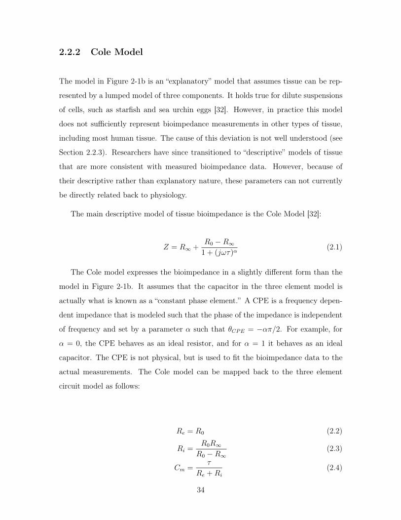
2.2.2 Cole Model
The model in Figure 2-1b is an “explanatory” model that assumes tissue can be rep-
resented by a lumped model of three components. It holds true for dilute suspensions
of cells, such as starfish and sea urchin eggs [32]. However, in practice this model
does not sufficiently represent bioimpedance measurements in other types of tissue,
including most human tissue. The cause of this deviation is not well understood (see
Section 2.2.3). Researchers have since transitioned to “descriptive” models of tissue
that are more consistent with measured bioimpedance data. However, because of
their descriptive rather than explanatory nature, these parameters can not currently
be directly related back to physiology.
The main descriptive model of tissue bioimpedance is the Cole Model [32]:
𝑍 = 𝑅∞ +𝑅0 −𝑅∞
1 + (𝑗𝜔𝜏)𝛼(2.1)
The Cole model expresses the bioimpedance in a slightly different form than the
model in Figure 2-1b. It assumes that the capacitor in the three element model is
actually what is known as a “constant phase element.” A CPE is a frequency depen-
dent impedance that is modeled such that the phase of the impedance is independent
of frequency and set by a parameter 𝛼 such that 𝜃𝐶𝑃𝐸 = −𝛼𝜋/2. For example, for
𝛼 = 0, the CPE behaves as an ideal resistor, and for 𝛼 = 1 it behaves as an ideal
capacitor. The CPE is not physical, but is used to fit the bioimpedance data to the
actual measurements. The Cole model can be mapped back to the three element
circuit model as follows:
𝑅𝑒 = 𝑅0 (2.2)
𝑅𝑖 =𝑅0𝑅∞
𝑅0 −𝑅∞(2.3)
𝐶𝑚 =𝜏
𝑅𝑒 + 𝑅𝑖
(2.4)
34

2.2.3 The 𝛼 Term
Measured bioimpedance data of human tissue does not match the three element circuit
model described in 2.2.1. Rather, the Cole model described in Section 2.2.2 is a better
approximation of the bioimpedance spectrum. Though parameters 𝑅0, 𝑅∞, and 𝜏
can be mapped back to the three element circuit model, the 𝛼 term does not have a
concrete physiological meaning. There have been many attempts to explain why the
term appears in bioimpedance data, but there is no agreement on its meaning.
Some researchers suggest that the 𝛼 term is caused by heterogeneity of cell sizes
and shapes in living tissue. This heterogeneity would result in a distribution of
relaxation times (i.e. time constants) that can produce a bioimpedance spectrum
that replicates the effect observed in tissue (see e.g. [33]). However, Ivorra et al.
argue that the amount of heterogeneity required to achieve an 𝛼 term of 0.8 (typical
for bioimpedance measurements), a non-physiologically broad distribution of cell sizes
and shapes would be required [34]. They provide some evidence that the 𝛼 term is
related to extracellular morphology; however, their experimental results do not fully
support their simulations.
2.2.4 Stray Capacitance in Bioimpedance Measurements
Bioimpedance measurements for fluid status are typically performed in a frequency
range of 1 kHz – 1 MHz. Unfortunately, as with all systems, bioimpedance measure-
ments have parasitic capacitances (referred to as “stray capacitance”) that impact
measurements at frequencies above 100 kHz. Any parasitics from the cabling and
instrumentation itself can be calibrated out, but stray capacitance from the body will
remain and needs to be accounted for.
The impact of the stray capacitance can be modeled as a capacitor in parallel
with the body (see Figure 2-3). This parallel capacitance causes significant negative
phase deviations at frequencies above 100 kHz (see Figure 2-4). The magnitude is
less affected by the stray capacitance, but can be impacted at frequencies above 500
kHz.
35

Figure 2-3: Stray capacitance in the bioimpedance measurement is in parallelwith the body impedance.
Because the magnitude of the impedance is less affected than the phase, one
approach to minimizing the impact of stray capacitance is to fit to only the magnitude.
Other possibilities include correcting for the stray capacitance in some fashion, and/or
extrapolating the desired parameters from lower frequency measurements.
2.3 Estimating Fluid Volume
While bioimpedance is related to volume status, it must be transformed to estimate
actual fluid volume. Fitting bioimpedance data to the Cole Model (Equation 2.1) re-
turns parameters 𝑅0, 𝑅∞, 𝛼 and 𝜏 , which can be readily converted to 𝑅𝑒, 𝑅𝑖, and 𝐶𝑚
from Figure 2-1b. However, 𝑅𝑒 and 𝑅𝑖 only indicate the resistance of the measured
tissue, rather than the fluid volume. In this section, the two main methods for esti-
mated fluid volume from measured resistance are presented: bioelectrical impedance
analysis (BIA) and bioimpedance spectroscopy (BIS).
2.3.1 Bioelectrical Impedance Analysis
BIA estimates TBW, ECW, and ICW for an individual from a population of simi-
lar individuals. Measurements include “whole body” (wrist-to-ankle) measurements
and “segmental” measurements (measurements of individual body segments such as
arm, trunk, leg, etc.) that are performed at a single frequency (SFBIA) or multiple
36

Figure 2-4: Calculated changes in magnitude and phase with the addition of straycapacitance values of 50 pF (red) and 100 pF (yellow). Stray capacitance acts inparallel with the body impedance and causes significant deviations in the phase athigh frequencies (red and yellow lines) when compared with no stray capacitance(blue line).
frequencies (MFBIA). SFBIA is typically measured at 50 kHz. MFBIA is measured
over a range of frequencies, typically from 1 kHz to 500 kHz.
Whole body BIA measurements assume that the body is a single conductive cylin-
der with homogeneous composition and constant geometry. The resistance of such a
cylinder is:
𝑅 =𝜌𝐻
𝐴(2.5)
where 𝜌 is the resistivity of the cylinder, H is the height of the individual (i.e.
the length of the cylinder), and A is the cross sectional area. This equation can be
rearranged to relate the resistance of the cylinder to the volume of the cylinder 𝑉 𝑜𝑙:
37
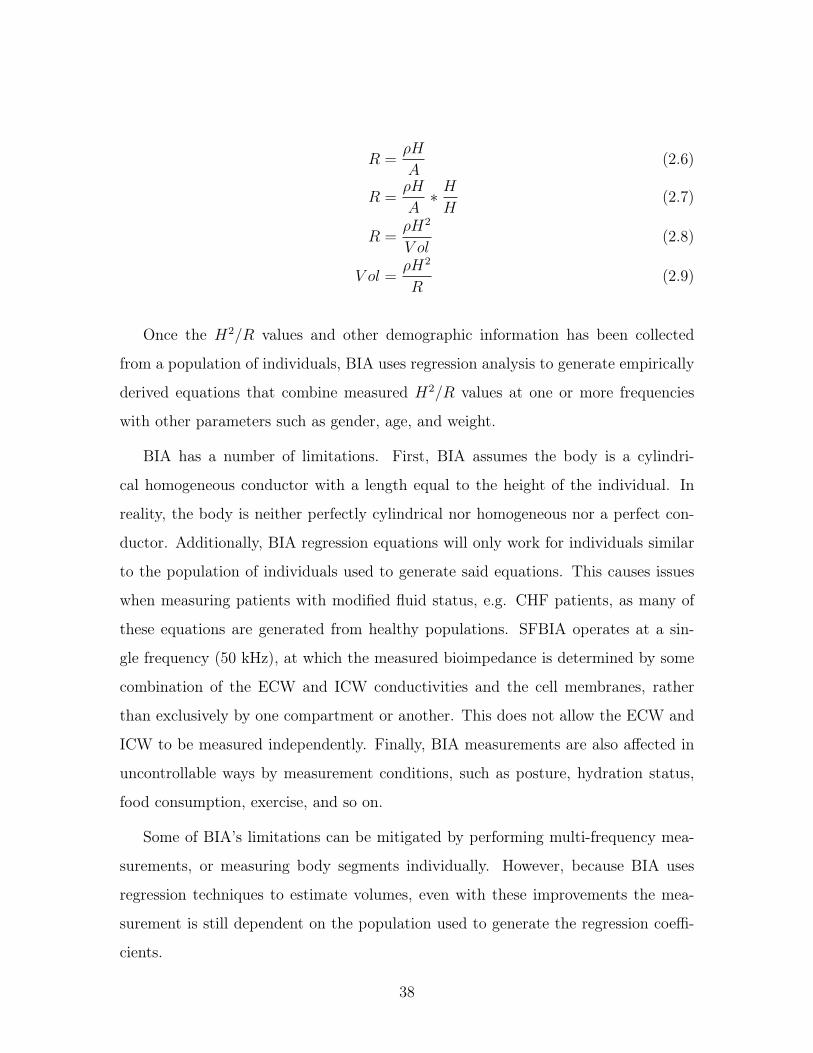
𝑅 =𝜌𝐻
𝐴(2.6)
𝑅 =𝜌𝐻
𝐴* 𝐻
𝐻(2.7)
𝑅 =𝜌𝐻2
𝑉 𝑜𝑙(2.8)
𝑉 𝑜𝑙 =𝜌𝐻2
𝑅(2.9)
Once the 𝐻2/𝑅 values and other demographic information has been collected
from a population of individuals, BIA uses regression analysis to generate empirically
derived equations that combine measured 𝐻2/𝑅 values at one or more frequencies
with other parameters such as gender, age, and weight.
BIA has a number of limitations. First, BIA assumes the body is a cylindri-
cal homogeneous conductor with a length equal to the height of the individual. In
reality, the body is neither perfectly cylindrical nor homogeneous nor a perfect con-
ductor. Additionally, BIA regression equations will only work for individuals similar
to the population of individuals used to generate said equations. This causes issues
when measuring patients with modified fluid status, e.g. CHF patients, as many of
these equations are generated from healthy populations. SFBIA operates at a sin-
gle frequency (50 kHz), at which the measured bioimpedance is determined by some
combination of the ECW and ICW conductivities and the cell membranes, rather
than exclusively by one compartment or another. This does not allow the ECW and
ICW to be measured independently. Finally, BIA measurements are also affected in
uncontrollable ways by measurement conditions, such as posture, hydration status,
food consumption, exercise, and so on.
Some of BIA’s limitations can be mitigated by performing multi-frequency mea-
surements, or measuring body segments individually. However, because BIA uses
regression techniques to estimate volumes, even with these improvements the mea-
surement is still dependent on the population used to generate the regression coeffi-
cients.
38

2.3.2 Bioimpedance Spectroscopy
The second commonly used bioimpedance volume estimation method is called bio-
impedance spectroscopy (BIS). BIS, as the name suggests, measures bioimpedance
over a range of frequencies, often 1 kHz to 1 MHz. Like BIA, BIS assumes the
body is cylindrical. However, rather than assuming the body is a single homogeneous
cylinder, BIS assumes the body consists of three conductive cylinders with different
dimensions in series: one for the arm, one for the leg, and one for the trunk [31].
For the calculation of ECW, three series cylinders are assumed to be filled with
conductive fluid and suspended non-conductive spherical elements (i.e. cells). The
apparent resistivity of such a suspension is:
𝜌𝑎 =𝜌
(1 − 𝑐)3/2(2.10)
where 𝜌 is the resistivity of the conductive fluid and c is a dimensionless volume
fraction of the non-conducting spheres. If the non-conducting spheres have a volume
equal to the ICW, c becomes:
𝑐 = 1 − 𝑉 𝑜𝑙𝐸𝐶𝑊
𝑉 𝑜𝑙𝐵(2.11)
where 𝑉 𝑜𝑙𝐸𝐶𝑊 is the volume of ECW in the cylinder and 𝑉 𝑜𝑙𝐵 is the total volume
of body (cylinder). Assuming the ECW has a resistivity 𝜌𝑒, the apparent resistivity
of the cylinder at low frequencies (cells non-conducting) is then:
𝜌𝑎𝑒 = 𝜌𝑒
(𝑉 𝑜𝑙𝐵
𝑉 𝑜𝑙𝐸𝐶𝑊
)3/2
(2.12)
Now assume each of the cylinders has the same resistivity 𝜌𝑎𝑒 (which, by definition,
requires a common 𝑉 𝑜𝑙𝐵𝑉 𝑜𝑙𝐸𝐶𝑊
ratio for each cylinder). The “total body” resistance is then
the sum of the resistance of each of the three cylinders:
𝑅𝑡𝑜𝑡𝑎𝑙 = 𝜌𝑎𝑒4𝜋
(𝐿𝑎
𝐶2𝑎
+𝐿𝑙
𝐶2𝑙
+𝐿𝑡
𝐶2𝑡
)(2.13)
where 𝐿𝑎 and 𝐶𝑎 are the length and circumference of the arm, respectively, 𝐿𝑙 and
39

𝐶𝑙 are the length and circumference of the leg, respectively, and 𝐿𝑡 and 𝐶𝑡 are the
length and circumference of the trunk, respectively. In practice and for simplicity’s
sake, however, standard BIS measurements use the height of the individual, and not
the lengths and circumferences of an arm, trunk, and leg. Instead, it is assumed that
human anthropometrics can be accounted for with a “shape factor” 𝐾𝑏. Then the
whole body resistance can be related to the volume as in Equation 2.8 multiplied by
𝐾𝑏:
𝑅 =𝐾𝑏𝜌𝑎𝑒𝐻
2
𝑉 𝑜𝑙𝐵(2.14)
where 𝐾𝑏 is a constant derived from anthropometric ratios usually assumed to
be 4.3 for all individuals [35], 𝐻 is the individual’s height, and 𝑉 𝑜𝑙𝐵 is the total
body volume. Plugging the expression of 𝜌𝑎𝑒 into Equation 2.14, the resistance of the
volume at low frequencies then becomes:
𝑅𝑒 = 𝐾𝑏𝐻2𝑉 𝑜𝑙
1/2𝐵 𝜌𝑒𝑉 𝑜𝑙
−3/2𝐸𝐶𝑊 (2.15)
and then the volume of ECW can be calculated as:
𝑉 𝑜𝑙𝐸𝐶𝑊 = 𝑘𝑒
(𝐻2𝑊 1/2
𝑅𝑒
)2/3
(2.16)
with:
𝑘𝑒 = 10−2
(𝐾𝑏𝜌𝑒
𝐷1/2𝑏
)2/3
(2.17)
where W is body weight (kg), H is height (cm), 𝜌𝑒 is the 𝜌 of ECW (Ω· cm), and
𝐷𝑏 is body density (kg/l).
For calculation of TBW, one could follow a procedure analogous to what has been
described for ECW, and obtain:
𝑉 𝑜𝑙𝑇𝐵𝑊 = 𝑘𝑡
(𝐻2𝑊 1/2
𝑅∞
)2/3
(2.18)
40

with:
𝑘𝑡 = 10−2
(𝐾𝑏𝜌∞
𝐷1/2𝑏
)2/3
(2.19)
where 𝜌𝐼𝐶𝑊 = 3 − 6𝜌𝐸𝐶𝑊 [36].
This method requires estimation of TBW resistivity 𝜌∞. There are multiple ap-
proaches to estimate this resistivity. One method is to assume it is linearly related to
ECW and ICW resistivities in proportion to their respective volumes [35,37]. Another
method is to assume 𝜌∞ is non-linearly related to the ECW and ICW resistivities,
and also related to the measured resistances 𝑅0 and 𝑅∞ (from [37,38]):
𝜌∞ = 𝜌𝐼𝐶𝑊 − (𝜌𝐼𝐶𝑊 − 𝜌𝐸𝐶𝑊 )
(𝑅∞
𝑅0
)2/3
(2.20)
In practice, it can be very difficult to determine the mean resistivity of ICW as
it varies depending on the type of cells. It may be most appropriate to determine 𝑘𝑡
empirically.
ICW is the most difficult compartment to estimate independently. It is repre-
sented by both the intracellular resistance 𝑅𝑖 and the membrane capacitance 𝐶𝑚,
so one cannot solve the analogous equations for ECW and TBW with the 𝑅𝑖 term.
Additionally, because the relationship of TBW resistivity and ECW/ICW ratio is
non-linear, these equations will not account for those effects. It appears that the best
way to calculate ICW is to subtract ECW from TBW (ICW = TBW - ECW) [37].
Like BIA, BIS relies on a number of assumptions. Some variables in the above
equations are measured, and others are assumed (see Table 2.1). Assumptions include
1) that the anthropometric factor 𝐾𝑏 is accurate for the patient, 2) that tissue behaves
like a mixture of non-conducting spheres in a conducting medium, 3) that the 𝑅𝑒 and
𝑅𝑖 extrapolated from measured bioimpedance data do in fact correspond to resistances
at DC and infinity frequency, 4) that the ECW and ICW are electrically homogeneous
fluids on a macroscopic scale, and 5) that the resistivities of the ECW and ICW are
known and constant.
BIS measurements tend to perform well in aggregate, though there are limitations
41

Var. Descr. Units Meas.? Male Female Ref.𝐾𝑏 Shape Factor unitless No 4.3 4.3 [35]𝜌𝑒 ECW Resistivity Ω cm No 40.3 42.3, 39.0 [37]𝜌∞ TBW Resistivity Ω cm No see Eq. 2.20 see Eq. 2.20 [38]𝐻 Height cm Yes n/a n/a n/a𝐷𝑏 Body Density kg/L No 1.05 1.05 [37]𝑅0 R @ DC Ω Yes n/a n/a n/a𝑅inf R @ ∞ Ω Yes n/a n/a n/a𝑊 Weight kg Yes n/a n/a n/a
𝑘𝑒 10−2
(𝐾𝑏𝜌𝑒
𝐷1/2𝑏
)2/3
unitless No 0.306 0.316 or 0.299 [37]
𝑘𝑡 10−2
(𝐾𝑏𝜌∞
𝐷1/2𝑏
)2/3
unitless No see Eq. 2.20 see Eq. 2.20 [37,38]
Table 2.1: Variables in BIS measurements.
in how well these measurements perform in any one individual [37]. Factors that
limit accuracy include similar factors that limit BIA accuracy (hydration, eating,
posture, etc.) and also the assumptions of the BIS models. BIS measurements may
be improved by performing segmental measurements, or by modifying the equations
presented in this section. However, even with a robust estimation of key BIS parame-
ters from over 170 patients, there are fundamental limitations to the BIS method [37].
Additionally, the effort of this estimation does not produce significantly better volume
estimates. According to Buendia et al., ECW estimation appears to be most limited
by the anisotropy inherent in actual tissue and TBW due to the uncertainty of 𝜌𝑖.
ICW estimated independently is limited by the issues described in a previous para-
graph in this section. Improvements to BIS do not seem likely without developing
entirely new models or techniques.
BIS may be good enough at estimating ECW, TBW, and ICW for CHF applica-
tions. However, a limitation of using standard BIS is the lack of a reference in order to
classify hydration status. Knowing an individual’s compartment volumes (i.e. ECW,
ICW, and TBW) does not make a statement as to whether that patient has excess
fluid or not, and so classification is necessary.
42
2.4 Classifying Patients Based on Bioimpedance Data
In the previous section, two methods of relating measured bioimpedance data to
volume were presented: bioelectrical impedance analysis (BIA) and bioimpedance
spectroscopy (BIS). The challenge with using BIA and BIS for management of CHF
is that even with knowledge of an individual’s fluid volumes (ECW/ICW/TBW), it
is challenging to determine whether that patient has excess fluid or not [39]. Ideally,
such a method would both determine whether a patient is fluid overloaded or not,
and if they are, by how much. In this section, methods for classifying patients based
on bioimpedance data will be presented. Some of these methods can be combined
with BIA/BIS, and others are standalone.
2.4.1 Bioelectrical Impedance Vector Analysis
Bioelectrical Impedance Vector Analysis is a single frequency measurement (usu-
ally 50 kHz) performed from hand-to-foot or on a body segment. BIVA measures
bioimpedance and compares a conductor length (i.e. height or segment length) nor-
malized bioimpedance value with a probabilistic distribution of fluid status to de-
termine whether a patient has fluid overload [40]. Patients with bioimpedance mea-
surements outside the 75% percentile are considered dehydrated or fluid overloaded
depending on the direction of the deviation.
BIVA assumes that an individual’s hydration state can be determined with respect
to a population with similar demographics. It also assumes that the phase angle is
accurate enough for proper characterization. BIVA suffers from some similar limi-
tations to that of standard BIA, including lack of differentiation between ECW and
ICW. Though BIVA allows for categorization with respect to a population, it does
not provide any estimate of how much fluid overload a patient has.
2.4.2 ECW/TBW ratio
The ECW/TBW ratio can be to classify patients as fluid-overloaded vs. normally
hydrated. It has been shown that CHF patients tend to have higher ECW/TBW ratio
43

than healthy participants [41]. A patient’s ECW/TBW ratio could be measured, for
example, using BIS techniques, and compared with a threshold determined from
healthy participants of a similar demographic.
The ECW/TBW ratio is independent of geometry. When calculating ECW and
TBW as indicated in Equations 2.16 and 2.18, the ratio reduces to a function of
resistivities and measured resistances:
𝑉 𝑜𝑙𝐸𝐶𝑊
𝑉 𝑜𝑙𝑇𝐵𝑊
=
(𝜌𝐸𝐶𝑊𝑅∞
𝜌∞𝑅𝑒
)2/3
(2.21)
Unfortunately, in practice, there are a wide range of “healthy” ECW/TBW ratios
[42]. This makes it difficult to use ECW/TBW ratio to determine any individual
person’s normal hydration status. ECW/TBW ratio can distinctly determine that an
individual is fluid overloaded if their ECW/TBW ratio is sufficiently high, but not
what a healthy number for that patient should be. ECW/TBW ratio seems like a
metric that may be useful to use in combination with other metrics, but not as a sole
classifier of fluid status.
2.4.3 Body Composition Monitor
One investigatory method to classify fluid overloaded patients is a technique that has
been integrated into a device called the Body Composition Monitor. This technique
uses regression methods to estimate the amount of fluid overload directly (i.e. the
equations are empirical from the patient population). It takes ECW and ICW volume
estimates from BIS measurements and the patient’s current weight, applies a regres-
sion based on data from a similar patient population, and outputs a fluid overload
estimate in liters. The fluid overload volume can then inform the ultrafiltration rate
or diuretic dosage for overloaded patients. One BCM equation used in the literature
is:
𝐹𝑂 = 1.136 * 𝑉 𝑜𝑙𝐸𝐶𝑊 − 0.43 * 𝑉 𝑜𝑙𝐼𝐶𝑊 − 0.114 *𝑊𝑝𝑟𝑒−𝐻𝐷 (2.22)
where 𝐹𝑂 is the total fluid overload, 𝑉 𝑜𝑙𝐸𝐶𝑊 and 𝑉 𝑜𝑙𝐼𝐶𝑊 are patient-specific
44

measured ECW and ICW volumes, and 𝑊𝑝𝑟𝑒−𝐻𝐷 is the weight pre-hemodialysis.
The BCM assumes that the fluid overload state of a patient can be determined from
a regression of similar patients. In practice, this appears to be performing well in
trials [43, 44], though more data from diverse populations is required. As with all
regression techniques, BCM is limited in its efficacy to the population used to generate
said regressions and the patient’s relationship to that population.
2.4.4 Healthy CNR Range
Figure 2-5: Electrode placement for the calf measurement used in [45].
The last method to be discussed in this section is a method introduced by Zhu et
al [45]. Unlike previous methods that measure complex bioimpedance at 50 kHz and
from hand-to-foot, this method measures 5 kHz resistance at the calf. The method
was developed for use with hemodialysis patients to determine their dry weight toward
the end of a session. The authors compare the calf normalized resistivity (CNR, calf
resistivity divided by body mass index) with measurements of healthy individuals’
CNR to verify the patient is in a healthy range (18.3 ·10−2Ω𝑀3𝑘𝑔−1 for male patients
and 20 · 10−2Ω𝑀3𝑘𝑔−1 for female patients).
Electrodes are placed in the middle of the calf with an inter-electrode distance
for the voltage electrodes of 10 cm (see Figure 2-5). The average calf circumference
is measured at the beginning and end of the hemodialysis session and used in com-
bination with the inter-electrode distance (10 cm) and the resistance at 5 kHz to
calculate the resistivity of the calf. Because the circumference of the calf will change
45

continuously throughout the course of the hemodialysis sessions, the authors derived
an equation to calculate the circumference during hemodialysis:
𝐶(𝑡) =
√𝐶(0)2 − 4𝜋𝜌(0)𝐿
𝑅(0)
(1 − 𝑅(0)
𝑅(𝑡)
)(2.23)
where 𝐶(0) and 𝑅(0) are the circumference and the low frequency resistance at the
start of the hemodialysis session, 𝜌(0) is a experimentally calibrated initial resistivity
of the calf, L is the inter-electrode distance (10 cm), and 𝐶(𝑡) and 𝑅(𝑡) are the
circumference and the low frequency resistance at time 𝑡.
The resistivity as a function of time is then:
𝜌(𝑡) =𝐶(𝑡)2 ·𝑅(𝑡)
4𝜋𝐿Ω 𝑐𝑚 (2.24)
The instantaneous calf resistivity 𝜌(𝑡) can be normalized by BMI (Weight / 𝐻2)
to obtain the calf normalized resistivity” (CNR). Resistivity is normalized by BMI
because body fat can impact the measurement, especially with a short inter-electrode
distance. A typical measurement is pictured in Figure 2-6.
This method assumes that the calf can be modeled as a cylinder with a uniform
resistivity. The method also assumes that fluid in the calf is the last segment to lose
its excess fluid, and so when the calf is in a healthy range, so is the rest of the body.
Zhu et al.’s method has been developed specifically for determining dry weight
in real-time during a hemodialysis session. In this sense, it has an advantage over
methods standard BIA, BIS, and BIVA in that those methods have been developed
for body composition in general, whereas this method was developed specifically for
determining fluid overload. Additionally, Zhu et al. argue that their method is
more robust than using the ECW/TBW ratio, as the ECW/TBW ratio has greater
variability. Placement at the calf does require the patient to keep one leg still for the
course of the session, but this is preferable compared to keeping an entire side still as
in the hand to foot cases.
One of the limitations of this method is that it cannot not estimate fluid overload
before the start of the hemodialysis session; it can only tell when a patient reaches a
46

Figure 2-6: Changes in calf normalized resistivity as a function of time duringa hemodialysis session (pink curve) [26]. The blue curve represents the currentmeasured resistance divided by the initial measured resistance.
healthy CNR range. In this sense, the Body Composition Monitor has an advantage
over this method. However, a recent paper suggests that it may be possible to use
CNR measurements to estimate fluid overload before the start of a hemodialysis
session [42].
2.5 Discussion
Two methods of volume estimation (Section 2.3) and four methods for classifying
patients and/or estimating dry weight (Section 2.4) have been presented. In this
section, the functional requirements of the BIS system to be developed in this thesis
will be re-examined, and the methods presented evaluated.
Recall the function requirements first outlined in Section 1.4. For translation to a
wearable form factor, it is important that a particular method satisfies the following:
1. Distinguish between ECW and ICW.
2. Accurately determine changes in ECW or its correlates.
3. Classify a patient’s hydration status.
47

4. Perform robustly in an every day setting.
5. Integrate with a wearable system.
6. Maintain patient comfort and compliance.
An evaluation of each of the methods presented in this thesis thus far, including the
two volume estimation methods (BIA and BIS), and the four classification methods
(BIVA, ECW/TBW ratio, BCM, and CNR), is presented in Table 2.2.
Functional Requirement 1 2 3 4 5 6Distinguish ECW and ICW No Yes No Yes Yes YesAccurately track ECW changes No Yes No Yes Yes Yes*Hydration classification No No Yes Yes Yes YesRobust Measurement Least Middle Least Middle Middle MostIntegration into wearable Least Least Least Least Least MostPatient compliance Least Least Least Least Least Most
Table 2.2: Functional Requirements of the evaluated methodologies. Methods: 1- BIA, 2 - BIS, 3 - BIVA, 4 - ECW/TBW ratio, 5 - BCM, 6 - CNR. * Method 6tracks ECW indirectly.
2.5.1 Distinguish ECW and ICW
Four out of the six methods (BIS, ECW/TBW ratio, BCM, and CNR) are capable
of distinguishing between ECW and ICW. This is particularly important because
fluid overload involves the expansion of the extracellular space. BIS, ECW/TBW
ratio, and BCM distinguish between ECW and ICW by measuring bioimpedance at
multiple frequencies. The CNR method distinguishes ECW by only measuring ECW.
It measures resistance at 5 kHz, which is a frequency at which most if not all of
current driven through the body flows through the extracellular space and around
cells. BIA and BIVA cannot distinguish between ECW because they typically only
measure bioimpedance at 50 kHz. Multiple and/or low frequency implementations of
these methods would be able to distinguish ECW.
48

2.5.2 Accurately Track ECW Changes
The same four methods that can distinguish between ECW and ICW can also track
ECW over time. In the case of BIS and its derivatives, this is achieved by performing
subsequent measurements and comparing the volume estimates to that of previous
estimates. The CNR estimate method measures ECW indirectly by comparing the
resistivity over time. It is not yet understood how well these technologies will be able
to track ECW changes over time in an ambulatory environment.
2.5.3 Hydration Classification
As described in Section 2.4, one requires more than volume alone to classify a patient
as fluid overloaded. BIA and BIS both cannot classify hydration status without
additional information. The other methods (BIVA, ECW/TBW ratio, BCM, CNR)
are all intended to classify patients and/or estimate fluid overload. BIVA classifies
patients based on population data from similar individuals. ECW/TBW ratio uses
a threshold to determine whether a patient is fluid-overloaded or not. BCM uses
equations derived from a similar patient population to estimate fluid overload in
an individual patient. Finally, the CNR method does not classify patients directly;
rather it determines when the patient has returned to healthy fluid status with real-
time monitoring of calf bioimpedance during a hemodialysis session.
2.5.4 Robust Measurement
In order for bioimpedance measurements to be practical in an ambulatory environ-
ment, the methods used have to be robust to changing conditions such as motion,
eating, temperature, etc. Unfortunately, all bioimpedance methods will be affected
somewhat by conditions such as food intake and exercise. However, methods that are
hand-to-foot are likely more affected than the CNR method, as it is only on the calf,
and most vital organs that influence bioimpedance measurements are in the trunk.
As for noise considerations, BIA and BIVA are both single frequency measure-
ments and can be considered the “least” robust. It seems it will be the most challeng-
49

ing to ensure robust measurements with only one data point. BIS and its derivatives
(ECW/TBW ratio and BCM) involve multiple frequency measurements. The data
are fitted, minimizing the impact of a small number of noisy data points. Additionally,
with an entire frequency spectrum, it is easier to determine whether the measurement
is “valid” or needs to be repeated.
Electrode placement presents another problem. In this case, the CNR is considered
to be the most robust, because the geometry of the calf in the region of measurement
is relatively uniform. It has been shown that the measurement is minimally sensitive
to electrode placement [45], and correlates well with gold standard hydration markers
such as the ECW volume (derived using sodium bromide dilution) divided by the
fat-free mass (derived from MRI) [42].
2.5.5 Integration into Wearable
Integrating a hand-to-foot measurement into a wearable appears to be the most chal-
lenging. It would require something like a suit that covered both the wrist and ankle,
or a way to complete the circuit to perform a measurement (such as touching the
hand or wrist to a contact on the leg). Calf measurements appear best suited for
integration into a wearable, as electrodes for measuring bioimpedance to derive CNR
and calf volumes could be integrated into a sock or a band.
2.5.6 Patient Compliance
The last functional requirement is patient compliance. It is difficult to assess patient
compliance without speaking with patients directly. However, similar to the wearable
functional requirement, it seems likely that integration into a sock or a band would
be most comfortable for the patient, and integrate into their daily life. Many CHF
patients already wear compression socks, and one could imagine them wearing a sock
with sensors inside.
50

2.5.7 Measurements in this Thesis
Given the discussion above, measurements in this thesis will be at the calf. A multi-
frequency measurement at the calf can measure calf extracellular water, calf intracel-
lular water, and calf total water, track volume changes over time, and afford a robust
measurement in a hopefully compliant form factor. Methods such as the BCM method
or the CNR method could be incorporated with these measurements to classify pa-
tients according to fluid status, and alert patients and physicians of decompensation,
ideally preventing hospitalization.
2.6 Chapter Summary
Bioimpedance measures the electrical properties of tissue, which can in turn be related
to compartment volumes. Bioimpedance measurement spectra can be modeled as a
three element circuit with two resistors and a constant phase element. Fluid volume
can be estimated using regression techniques (Bioimpedance Analysis) or by using the
high and low frequency resistances with equations for resistivity of a suspension of cells
(Bioimpedance Spectroscopy). Fluid volumes alone are not sufficient to determine
whether a patient has fluid overload and classification is needed. Classification can
be achieved using probabilistic diagrams (Bioimpedance Vector Analysis), regression
(Body Composition Monitor), compartment ratios (ECW/TBW), and/or by tracking
normalized calf resistivity over time (Healthy CNR range). Measurements can be
performed from wrist-to-ankle or on a specific body segment. It was determined that
multi-frequency, calf based measurements are preferred for this thesis, as they are
more robust to changes in electrode placement in a hopefully more compliant form
factor.
51

52

Chapter 3
Fluid Status Changes in the Calf
During Hemodialysis
This Chapter addresses Aim 1 of the thesis: how are calf bioimpedance changes
measured during hemodialysis related to fluid removed during hemodialysis?
3.1 Introduction to Hemodialysis
3.1.1 The Process of Hemodialysis
Hemodialysis is a therapy used when patients have impaired renal function. A filter
known as a dialyzer acts as an artificial kidney that removes waste products and fluid
from the blood (see Figure 3-1). The dialyzer is a semipermeable membrane that is
filled with a solution called dialysate. Standard hemodialysis today consists of two
processes: diffusive hemodialysis for the removal of solutes, and ultrafiltration for
the removal of fluid and solutes using a pressure gradient. Blood is removed from
the body, filtered, and then returned back to the body, plus/minus solutes diffused
across the dialyzer membrane, and minus fluid and solutes removed by ultrafiltration.
This section will provide an overview for the fluid and solute shifts that occur during
hemodialysis.
53
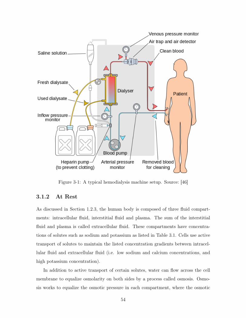
Figure 3-1: A typical hemodialysis machine setup. Source: [46]
3.1.2 At Rest
As discussed in Section 1.2.3, the human body is composed of three fluid compart-
ments: intracellular fluid, interstitial fluid and plasma. The sum of the interstitial
fluid and plasma is called extracellular fluid. These compartments have concentra-
tions of solutes such as sodium and potassium as listed in Table 3.1. Cells use active
transport of solutes to maintain the listed concentration gradients between intracel-
lular fluid and extracellular fluid (i.e. low sodium and calcium concentrations, and
high potassium concentration).
In addition to active transport of certain solutes, water can flow across the cell
membrane to equalize osmolarity on both sides by a process called osmosis. Osmo-
sis works to equalize the osmotic pressure in each compartment, where the osmotic
54

Substance and Units ECW ICW*Na+ (mEq/L) 140 14K+ (mEq/L) 4 120Ca2+, ionized (mEq/L) 2.5 1𝑒−4
Cl− (mEq/L) 105 10HCO−
3 (mEq/L) 24 10pH 7.4 7.1Osmolarity (mOsm/L) 290 290
Table 3.1: Major solutes in ECW and ICW. * The major anions of ICW areproteins and organic phosphates not included in the table. Table adapted from[47]. Solute concentrations are expressed in milliequivalents per liter (mEq/L). Amilliequivalent (mEq) is 10−3 times the number of moles of the solute multipliedby its valence. For example, one mole of NaCl in solution dissociates into oneequivalent of Na+ and one equivalent of Cl−. An osmole (osm) is the number ofparticles into which a solute dissociates in solution. For the case of NaCl, theosmolarity for 1 mmol/L NaCl is 2 mOsm/L.
pressure (𝜋) is defined as:
𝜋 = CRT (3.1)
where C is the concentration of solutes in osmoles per liter, R is the ideal gas
constant, and T is the absolute temperature in kelvin.
Permeant vs. Impermeant Solutes
The properties of different solutes within each compartment affect how they change
compartment volumes. Solutes in the body can be permeant or impermeant. Per-
meant solutes move across the cell membrane by a process called diffusion, which
is a function of the concentration gradient across the membrane. Permeant solute
concentrations will eventually settle to their equilibrium values with time and there-
fore increasing or decreasing the number of permeant solutes will not cause changes
in fluid shifts at equilibrium. However, permeant solutes may cause transient fluid
shifts as water flows more quickly than the concentration of most solutes equilibrate.
Impermeant solutes, on the other hand, do not move freely across membranes. Ad-
dition or subtraction of an impermeant solute will result in changes in compartment
55

volumes at equilibrium.
In cells, proteins are impermeant. Additionally, because the concentration of
solutes like sodium, potassium, and calcium are controlled by active processes, one
can consider these solutes impermeant as well. The waste product urea is permeant.
In extracellular fluid, the interstitial fluid contains sodium, potassium, calcium, and
urea (all permeant), and the plasma contains sodium, potassium, calcium, and urea
as permeant solutes and proteins as impermeant solutes.
3.1.3 Diffusive Hemodialysis
Diffusive hemodialysis involves the removal of waste products such as urea and the
adjustment of plasma sodium and potassium concentrations as needed. Sodium and
potassium will move in or out of the plasma depending on the concentration gradient
between the dialysate and the plasma (see Figure 3-2). There is also a large gradient
to move urea and creatinine out of the plasma.
During diffusive hemodialysis, permeant solutes begin to diffuse across the various
membranes. If the concentration of dialysate sodium and potassium are in equilibrium
with plasma concentrations, there will be no changes in compartment volumes at
equilibrium. However, the diffusion of permeant solutes such as urea can transiently
shift fluid into and out of cells. Consider for example, the simplified case of a system
with only sodium and urea. The concentration of sodium is at equilibrium across all
membranes (see Figure 3-3). As urea is cleared by the dialyzer, the osmolarity of the
extracellular space decreases. Urea will begin diffusing across the cell membranes to
increase the osmolarity of the extracellular fluid, but water will begin to flow first and
faster, leading to a transient fluid shift from the extracellular space to the intracellular
space. This fluid shift causes an increase in extracellular osmolarity, which induces
a fluid shift back out of cells. The net effect can be a small increase in intracellular
fluid that dissipates over the course of the session and is completely eliminated after
the session.
Mismatched solute concentrations such as that of sodium, for example, can result
in increases or decreases in solute concentrations that can influence compartment vol-
56
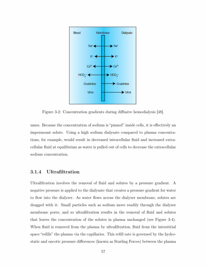
Figure 3-2: Concentration gradients during diffusive hemodialysis [48].
umes. Because the concentration of sodium is “pinned” inside cells, it is effectively an
impermeant solute. Using a high sodium dialysate compared to plasma concentra-
tions, for example, would result in decreased intracellular fluid and increased extra-
cellular fluid at equilibrium as water is pulled out of cells to decrease the extracellular
sodium concentration.
3.1.4 Ultrafiltration
Ultrafiltration involves the removal of fluid and solutes by a pressure gradient. A
negative pressure is applied to the dialysate that creates a pressure gradient for water
to flow into the dialyzer. As water flows across the dialyzer membrane, solutes are
dragged with it. Small particles such as sodium move readily through the dialyzer
membrane pores, and so ultrafiltration results in the removal of fluid and solutes
that leaves the concentration of the solutes in plasma unchanged (see Figure 3-4).
When fluid is removed from the plasma by ultrafiltration, fluid from the interstitial
space “refills” the plasma via the capillaries. This refill rate is governed by the hydro-
static and oncotic pressure differences (known as Starling Forces) between the plasma
57

Figure 3-3: Fluid flow during diffusive hemodialysis.
volume and the interstitial space as:
𝐽 = 𝐿𝑝𝑆([𝑃𝑐 − 𝑃𝑖] − 𝜎[𝜋𝑐 − 𝜋𝑖]) (3.2)
where 𝐽 is the net flow with positive 𝐽 indicating flow out of capillaries, 𝐿𝑝 is the
hydraulic conductivity of the membrane, 𝑆 is the surface area for filtration, 𝑃𝑐 − 𝑃𝑖
is the hydrostatic pressure gradient between the capillaries and the interstitial space,
𝜎 is the reflection coefficient, and 𝜋𝑐−𝜋𝑖 is the oncotic pressure gradient between the
capillaries and the interstitial space. Hydrostatic pressure is the pressure of blood
against the vessel walls, and oncotic pressure is a form of osmotic pressure exerted
specifically by proteins.
Fluid removal from the plasma reduces plasma hydrostatic pressure and increases
plasma oncotic pressure (proteins are too large to pass through the dialyzer), which
induces fluid flow into plasma at a rate called the “plasma refill rate.” As fluid leaves
the interstitial space, the interstitial osmolarity increases. With time, solutes will
diffuse from the interstitial space to the plasma to reduce the osmolarity gradient.
58

Figure 3-4: Fluid flow during isolated ultrafiltration. OP = oncotic pressure, HP= hydrostatic pressure.
However, if the ultrafiltration rate is sufficiently fast, fluid will temporarily flow out
from cells in order to reduce the interstitial osmolarity.
3.1.5 Combined Hemodialysis
Combined hemodialysis involves both diffusion and ultrafiltration. The resulting
compartment volume shifts will depend on fluid and solute shifts induced by each
process. Fluid flow in or out of cells, for example, will be determined by a combination
of three mechanisms: 1) Urea that freely diffuses across the cell membrane, which
induces a small transient fluid shift into cells, 2) dialysate concentrations that induce
fluid shifts in or out of cells depending on the concentration gradient with respect to
the dialyzer, and 3) transient fluid shifts out of cells that occur at sufficiently high
ultrafiltration rates. Fluid flow in or out of the interstitial space will be governed by a
combination of the Starling forces and the intracellular fluid shifts. Finally, fluid flow
in or out of the plasma will be governed by ultrafiltration and the Starling Forces.
59

3.1.6 Calf Bioimpedance Changes During Hemodialysis
Previous literature measuring changes in bioimpedance during hemodialysis have
found that the leg is disproportionately recruited for fluid removal as compared with
the trunk and arms in routine hemodialysis patients [49–53]. Additionally, Zhu et al.
have documented that the leg tends to empty last, making the calf an ideal measure-
ment location for determining a patient has reached a healthy fluid status [26, 51].
These studies cite one or both of two hypotheses to explain this presentation: 1)
differences in regional blood flow and 2) a greater amount of fluid overload in the leg
relative to other parts of the body. It has also been hypothesized that the fluid from
the calf is recruited to refill the trunk [51].
3.2 Clinical Testing Methods
The goal of clinical testing was to relate changes in calf bioimpedance to fluid removed
during hemodialysis. Calf bioimpedance measurements were performed with patients
presenting to the Massachusetts General Hospital (MGH) Inpatient Units undergoing
hemodialysis using a commercial measurement system (Impedimed SFB7). Patient
vital signs, calf circumference, relevant hemodialysis parameters, and relevant patient
information were also recorded. All patients received standard clinical care, including
routine clinical assessments, laboratory testing, and diagnostic imaging.
3.2.1 Inclusion / Exclusion Criteria
Inclusion criteria:
1. Age > 18 years
2. Inpatients undergoing hemodialysis
Exclusion criteria:
1. Pregnant women
2. Inability to consent
60

3. Amputations
4. Metal in body (in current path and/or active device)
5. Inability to place electrodes at test location (calf)
Inclusion criteria were intentionally broad to increase the rate of patient recruit-
ment, which at times even with these criteria could be less than one scheduled
patient every two weeks. Exclusion criteria were driven by concerns for patient
safety/ethics (pregnant women, inability to consent), or concerns about an influence
on the bioimpedance measurements (metal in body, inability to place electrodes) or
patient circulation (amputations).
3.2.2 Study Procedures
After the patient gave informed consent, the researcher attended the patient’s next
hemodialysis session. Upon patient arrival, nursing staff assisted the patient in per-
forming a standing weight (referred to as the patient’s “Initial Weight”). The patient
then laid back down on a bed in a “semi-supine” position with their legs at the same
level as their buttocks and their torso slightly elevated on pillows. Four Ag/AgCl elec-
trodes were placed on the side of the patient’s calf (see Figure 3-5). The researcher
measured the distance between the middle of the patella (knee) and lateral malleolus
(ankle) and placed the voltage electrodes 5 cm on either side of the midpoint of this
distance. Current electrodes were placed 5 cm outside each voltage electrode.
The patient was allowed to choose which leg the electrodes were placed on. After
electrodes were placed on the patient, the calf circumference was measured at the
location of each voltage electrode. The mean of these two measurements was used in
subsequent analyses. After the calf circumference was measured, five measurements
were performed with a commercial bioimpedance spectroscopy measurement system
(Impedimed SFB7). All inputs / outputs (blood draws, eating/drinking) and rele-
vant vital signs (blood pressure, and heart rate and blood oxygenation when available)
were recorded throughout the session. At the end of the session, the experimental
61

Figure 3-5: Electrodes are placed along the side of the calf. The inner electrodesare voltage electrodes spaced 5 cm on either side of the “center” of the calf, definedas half the distance between the center of the patella and the center of the fibularprotrusion at the ankle. The outer electrodes are current electrodes that arespaced 5 cm apart from the inner electrodes. The positive current and voltageelectrodes are the more proximal pair of electrodes and the negative current andvoltage electrodes are the more distal pair.
system was removed from the patient and an additional five measurements were per-
formed with the commercial system. The calf circumference was measured again and
the patient performed another standing weight (referred to as the patient’s “Final
Weight”).
3.2.3 Calculating Bioimpedance Parameters
Bioimpedance parameters were extracted using MATLAB’s lsqcurvefit algorithm,
which performed a non-linear least squares fit to the Cole model (see Section 2.2.2).
The magnitude of the impedance was selected as input data and fitted to the Cole
62

model with the parameters 𝑅0, 𝑅∞, 𝜏, and 𝛼. The lsqcurvefit algorithm implemen-
tation allows the user to specify lower/upper bounds and starting values for each
parameter. The lower/upper bounds were configured as follows:
15 ≤𝑅0 ≤ 100 Ω (3.3)
15 ≤𝑅∞ ≤ 100 Ω (3.4)1
80 𝑘𝐻𝑧 * 2𝜋≤𝜏 ≤ 1
20 𝑘𝐻𝑧 * 2𝜋𝑠 (3.5)
0.65 ≤𝛼 ≤ 1 (3.6)
with starting values of:
𝑅0 = 60 Ω (3.7)
𝑅∞ = 20 Ω (3.8)
𝜏 =1
50 𝑘𝐻𝑧 * 2𝜋𝑠 (3.9)
𝛼 = 0.8 (3.10)
These bounds were selected both to constrain parameters to their possible physi-
cal values (in this case, all parameters must be positive), and to constrain parameters
to an empirically determined “physiological range.” For example, the 𝛼 parameter
bounds were originally set to 0 ≤ 𝛼 ≤ 1, but in some cases this resulted in 𝛼 param-
eters outside a physiological range, so the lower bound was increased to 0.65. The
resistive upper bounds were set assuming all fitted bioimpedance data was measured
at the calf, which in the measured patient population did not result in an 𝑅0 value
greater than 80 Ω. The bounds of both 𝑅0 and 𝑅∞ were set to be the same, though
technically 𝑅∞ should be strictly less than 𝑅0. The 𝜏 parameter was set assuming
that the time constant associated with 𝜏 must be in the range of 20 kHz and 80 kHz,
which allows for a 30 kHz deviation around the nominal value of 50 kHz. The starting
63

values were selected based on an actual bioimpedance measurement performed at the
calf in a healthy participant.
3.2.4 Calculating Calf Volumes
Calf Volume Abbreviations
As described in Section 1.2.3, the body is divided into extra- and intracellular fluid
(abbreviated ECW and ICW, respectively), the sum of which equals the total body
water (abbreviated TBW). When measuring bioimpedance in the calf, compartment
volumes will also consist of extra- and intracellular fluid for that measured volume.
For clarity, any reference to calf volumes will have a small c in front: calf extracellular
water is abbreviated cECW, calf intracellular water is abbreviated cICW, and calf
total water is abbreviated cTW.
Calculating cECW
The main difference between calculation of compartment volumes in the calf versus
the whole body (see Section 2.3) is that the calf is a single cylinder of known length
rather than three cylinders with a total length equal to the patient’s height. To
calculate cECW it is assumed that the cECW is the only contributing factor to the
resistance at low frequencies (i.e. 𝑅0), and that the measured volume is a single
conductive cylinder with homogeneous composition and constant geometry. In this
case the resistance of such a cylinder is:
𝑅0 =𝜌𝐿
𝐴(3.11)
where 𝜌 is the resistivity of the cylinder, L is the length of the segment, and A is
the cross sectional area. By multiplying the right half of the equation by 𝐿/𝐿, this
equation can relate the resistance of the cylinder to its volume:
64

𝑅0 =𝜌𝐿
𝐴(3.12)
𝑅0 =𝜌𝐿
𝐴* 𝐿
𝐿(3.13)
𝑅0 =𝜌𝐿2
𝑉 𝑜𝑙𝑐𝑎𝑙𝑓(3.14)
𝑉 𝑜𝑙𝑐𝑎𝑙𝑓 =𝜌𝐿2
𝑅0
(3.15)
where 𝑉 𝑜𝑙𝑐𝑎𝑙𝑓 = 𝐿 * 𝐴. Calculating the resistivity of the cylinder will allow the
measured resistance to be related specifically to the cECW volume.
The apparent resistivity of a medium filled with conductive fluid and suspended
non-conductive spherical elements is:
𝜌 =𝜌𝐸𝐶𝑊
(1 − 𝑐)3/2(3.16)
where 𝜌𝐸𝐶𝑊 is the resistivity of the conductive fluid and c is a dimensionless
volume fraction of the nonconducting spheres [54]. A typical value for 𝜌𝐸𝐶𝑊 is
40.5 Ω 𝑐𝑚 [36].1 If one assumes only the cECW is conducting at low frequencies,
c becomes:
𝑐 = 1 − 𝑉 𝑜𝑙𝑐𝐸𝐶𝑊
𝑉 𝑜𝑙𝑐𝑎𝑙𝑓(3.17)
where 𝑉 𝑜𝑙𝑐𝐸𝐶𝑊 is the volume of the cECW in the cylinder. Plugging in Equation
3.17 to Equation 3.16, the resistivity of the cylinder becomes:
𝜌 = 𝜌𝐸𝐶𝑊
(𝑉 𝑜𝑙𝑐𝑎𝑙𝑓𝑉 𝑜𝑙𝑐𝐸𝐶𝑊
)3/2
(3.18)
By plugging in the resistivity to Equation 3.11, 𝑉 𝑜𝑙𝑐𝐸𝐶𝑊 can be solved for:
𝑉 𝑜𝑙𝑐𝐸𝐶𝑊 =
(𝐿2𝜌𝐸𝐶𝑊
√𝑉 𝑜𝑙𝑐𝑎𝑙𝑓
𝑅0
)2/3
(3.19)
1There may be small changes in 𝜌𝐸𝐶𝑊 over the course of the hemodialysis session. See AppendixA for an analysis of how these changes affect measured results.
65

Calculating cTW
An analogous approach can be used to solve for cTW. The resistance at high frequen-
cies 𝑅∞ can be related to the volume by:
𝑅∞ =𝜌𝐿2
𝑉 𝑜𝑙𝑐𝑎𝑙𝑓(3.20)
with
𝜌 =𝜌∞
(1 − 𝑐)3/2(3.21)
If 𝑐 = 1 − 𝑉 𝑜𝑙𝑐𝑇𝑊
𝑉 𝑜𝑙𝑐𝑎𝑙𝑓, the cTW volume is:
𝑉 𝑜𝑙𝑐𝑇𝑊 =
(𝐿2𝜌∞
√𝑉 𝑜𝑙𝑐𝑎𝑙𝑓
𝑅0
)2/3
(3.22)
where 𝜌∞ has been shown by Matthie et al. to be [38]:
𝜌∞ = 𝜌𝐼𝐶𝑊 − (𝜌𝐼𝐶𝑊 − 𝜌𝐸𝐶𝑊 )
(𝑅∞
𝑅0
)2/3
(3.23)
where 𝜌𝐼𝐶𝑊 = 4.5𝜌𝐸𝐶𝑊 . The value of 4.5𝜌𝐸𝐶𝑊 was selected because results from
different studies range between 3 to 6 times 𝜌𝐸𝐶𝑊 [36]. A change of 𝜌𝐼𝐶𝑊 to 3𝜌𝐸𝐶𝑊
or 6𝜌𝐸𝐶𝑊 would change 𝑉 𝑜𝑙𝑐𝑇𝑊 by -10% and 10%, respectively. It would change
𝑉 𝑜𝑙𝑐𝐼𝐶𝑊 by -25% and 25%, respectively.
Calculating cICW
It is assumed that:
𝑐𝐼𝐶𝑊 = 𝑐𝑇𝑊 − 𝑐𝐸𝐶𝑊 (3.24)
A change of 𝜌𝐼𝐶𝑊 to 3𝜌𝐸𝐶𝑊 or 6𝜌𝐸𝐶𝑊 would change 𝑉 𝑜𝑙𝑐𝐼𝐶𝑊 by -25% and 25%,
respectively.
66

Measuring the “Total Volume” of the Calf
The compartment calculations in the previous sections use a volume 𝑉 𝑜𝑙𝑐𝑎𝑙𝑓 = 𝐿 *𝐴.
In the present measurements, 𝐿 is assumed to be 10 cm, which is the inter-electrode
distance of the voltage pickup electrodes placed on the calf (see Figure 3-5). If
one assumes the calf is a cylinder, the cross-sectional area can be related to the
circumference by:
𝐴 =𝑐𝑖𝑟𝑐2
4𝜋(3.25)
For this testing, the circumference 𝑐𝑖𝑟𝑐 is the average of the circumference mea-
surement at each voltage electrode.
3.2.5 Evaluation of Fluid Status
Three different metrics were used to assess patient fluid status: total body fluid over-
load, pedal edema, and calf normalized resistivity. Total fluid overload was calculated
as the difference between the patient’s weight at the start of the hemodialysis session
and a clinician’s assessment of a patient’s estimated dry weight (EDW) as obtained
from patient medical records. The clinician performs this assessment using a com-
bination of vital signs, physical exam, symptoms, labs and/or imaging. The fluid
overload can be calculated using the patient’s weight and their EDW as:
Fluid Overload (kg) = Initial Weight (kg) − Estimated Dry Weight (kg) (3.26)
Pedal edema was scored on a scale of 0 to 3 by clinicians (also as obtained from pa-
tient medical records), where: 0 = no visible edema, 1 = trace edema, 2 = significant
edema, and 3 = pitting edema. The assessment was made based on a combination of
visual inspection and palpation.
Finally, the calf normalized resistivity (CNR) was calculated as a metric of hy-
67
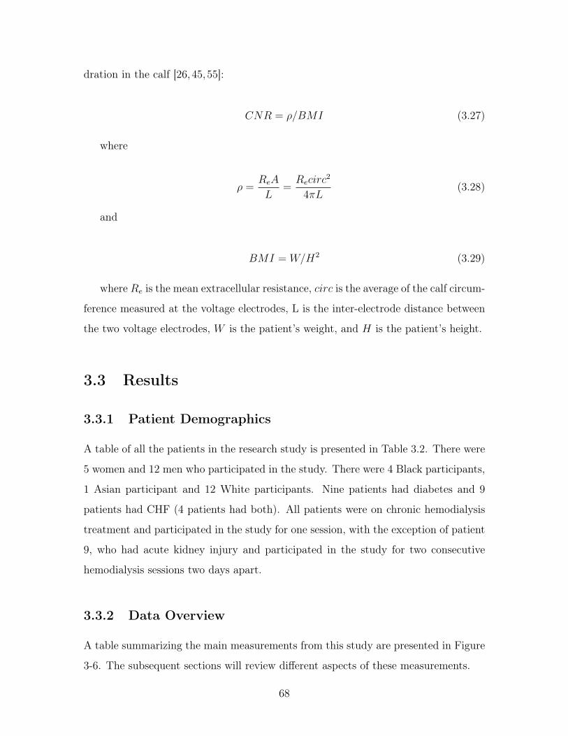
dration in the calf [26, 45,55]:
𝐶𝑁𝑅 = 𝜌/𝐵𝑀𝐼 (3.27)
where
𝜌 =𝑅𝑒𝐴
𝐿=
𝑅𝑒𝑐𝑖𝑟𝑐2
4𝜋𝐿(3.28)
and
𝐵𝑀𝐼 = 𝑊/𝐻2 (3.29)
where 𝑅𝑒 is the mean extracellular resistance, 𝑐𝑖𝑟𝑐 is the average of the calf circum-
ference measured at the voltage electrodes, L is the inter-electrode distance between
the two voltage electrodes, 𝑊 is the patient’s weight, and 𝐻 is the patient’s height.
3.3 Results
3.3.1 Patient Demographics
A table of all the patients in the research study is presented in Table 3.2. There were
5 women and 12 men who participated in the study. There were 4 Black participants,
1 Asian participant and 12 White participants. Nine patients had diabetes and 9
patients had CHF (4 patients had both). All patients were on chronic hemodialysis
treatment and participated in the study for one session, with the exception of patient
9, who had acute kidney injury and participated in the study for two consecutive
hemodialysis sessions two days apart.
3.3.2 Data Overview
A table summarizing the main measurements from this study are presented in Figure
3-6. The subsequent sections will review different aspects of these measurements.
68

Patient Sex Age H (cm) IW (kg) Race Leg DM CHF1 F 71 163 113.5 White R 1 12 M 62 178 93.7 White R 0 13 M 62 178 85.0 White L 0 14 F 58 163 74.1 Black R 1 15 M 66 185 99.8 White R 1 06 M 67 175 59 White R 0 17 M 56 188 127.4 White L 1 08 M 51 173 83.6 Black L 0 19 M 43 188 80.2 White R 0 010 M 74 180 56.3 Black R 0 011 F 88 155 57.9 White R 0 112 M 59 178 104.9 White L 1 013 M 65 168 73.3 White R 1 114 M 56 163 71.1 Black R 1 015 M 66 175 103.7 White R 1 116 F 70 160 53.3 White R 0 017 F 66 155 72.7 Asian R 1 0
Table 3.2: Patient demographics for all patients included in the clinical testing.H = height (cm), IW = initial weight (kg), DM = diabetes mellitus, CHF =congestive heart failure.
3.3.3 Ultrafiltration Measurement Reliability
Patients undergoing hemodialysis have fluid removed from the vasculature by a hemo-
dialysis machine. The hemodialysis machine displays the rate of fluid removal (ul-
trafiltration rate or UFR) and the total amount of fluid removed during the ses-
sion (ultrafiltration volume or UFV). It is important to determine the reliability of
the recorded ultrafiltration measurements before they are used as a metric of fluid
status changes. Two comparisons are performed in this section: 1) the predicted
UFV removed as determined by UFRs is compared with the recorded UFV from the
hemodialysis machine at the end of the session, and 2) the predicted weight change es-
timated from recorded inputs/outputs is compared with the measured weight change
over the course of the hemodialysis session.
69

Figure 3-6: Fluid status indicators, fluid removal, and bioimpedance changesfor all patients. FO = fluid overload, UFV = ultrafiltration volume, CNR =calf normalized resistivity. Data points in bold indicate negative bioimpedancechanges that are discussed in Section 3.3.10.
Predicted vs. Recorded Ultrafiltration Volume
The UFR is set at the beginning of the session and may change throughout the course
of the session. It is displayed in real-time on the hemodialysis machine, along with
the total UFV. For example, one patient started the session with a UFR of 940 ml/h,
and the UFR was increased an hour before the end of the session to 1160 ml/h (see
Table 3.3 and Figure 3-7). The predicted UFV is obtained by discrete integration of
the UFR over time at one second intervals. The recorded and predicted UFV for each
patient was consistent within ±5% for 16/18 patient runs, and within ±10% for the
other two patients (see Table 3.4). The larger % difference for the latter two patients
appears to be due to an incorrect recording of the time of a UFR change.
Predicted vs. Recorded Weight
A patient’s weight change between the beginning and end of the hemodialysis ses-
sion can be predicted using the UFV and other inputs and outputs that occur over
70

Time Rate (ml/h) Predicted (ml) Recorded (ml) Difference (%)7:34:49 940 0 0 010:01:11 1160 2293 2300 -0.3011:03:54 0 3506 3500 0.17
Table 3.3: An example UFR table used to determine the researcher’s accuracy inrecording UFR and UFV during the session.
07:00 08:00 09:00 10:00 11:00 12:00Time
0
500
1000
1500
2000
2500
3000
3500
4000
Tota
l U
FV
Rem
oved (
ml)
UFV removed versus time - HEM010
Predicted
Recorded
Figure 3-7: An example graph showing the consistency of the predicted vs.recorded UFV during a hemodialysis session.
71
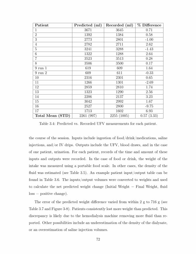
Patient Predicted (ml) Recorded (ml) % Difference1 3671 3645 0.712 1392 1384 0.583 2773 2801 -1.004 2782 2711 2.625 3241 3288 -1.436 1322 1288 2.647 3523 3513 0.288 3506 3500 0.179 run 1 619 609 1.649 run 2 609 611 -0.3310 2316 2301 0.6511 1266 1301 -2.6912 2859 2810 1.7413 1323 1290 2.5614 2206 2137 3.2315 3042 2992 1.6716 2527 2800 -9.7517 1713 1602 6.93Total Mean (STD) 2261 (997) 2255 (1005) 0.57 (3.33)
Table 3.4: Predicted vs. Recorded UFV measurements for each patient.
the course of the session. Inputs include ingestion of food/drink/medications, saline
injections, and/or IV drips. Outputs include the UFV, blood draws, and in the case
of one patient, urination. For each patient, records of the time and amount of these
inputs and outputs were recorded. In the case of food or drink, the weight of the
intake was measured using a portable food scale. In other cases, the density of the
fluid was estimated (see Table 3.5). An example patient input/output table can be
found in Table 3.6. The inputs/output volumes were converted to weights and used
to calculate the net predicted weight change (Initial Weight − Final Weight, fluid
loss = positive change).
The error of the predicted weight difference varied from within 2 g to 716 g (see
Table 3.7 and Figure 3-8). Patients consistently lost more weight than predicted. This
discrepancy is likely due to the hemodialysis machine removing more fluid than re-
ported. Other possibilities include an underestimation of the density of the dialysate,
or an overestimation of saline injection volumes.
72
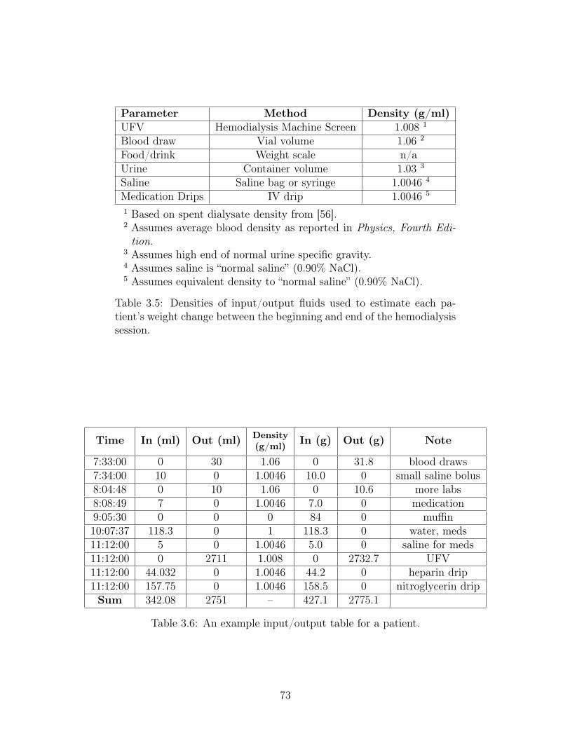
Parameter Method Density (g/ml)UFV Hemodialysis Machine Screen 1.008 1
Blood draw Vial volume 1.06 2
Food/drink Weight scale n/aUrine Container volume 1.03 3
Saline Saline bag or syringe 1.0046 4
Medication Drips IV drip 1.0046 5
1 Based on spent dialysate density from [56].2 Assumes average blood density as reported in Physics, Fourth Edi-tion.
3 Assumes high end of normal urine specific gravity.4 Assumes saline is “normal saline” (0.90% NaCl).5 Assumes equivalent density to “normal saline” (0.90% NaCl).
Table 3.5: Densities of input/output fluids used to estimate each pa-tient’s weight change between the beginning and end of the hemodialysissession.
Time In (ml) Out (ml) Density(g/ml) In (g) Out (g) Note
7:33:00 0 30 1.06 0 31.8 blood draws7:34:00 10 0 1.0046 10.0 0 small saline bolus8:04:48 0 10 1.06 0 10.6 more labs8:08:49 7 0 1.0046 7.0 0 medication9:05:30 0 0 0 84 0 muffin10:07:37 118.3 0 1 118.3 0 water, meds11:12:00 5 0 1.0046 5.0 0 saline for meds11:12:00 0 2711 1.008 0 2732.7 UFV11:12:00 44.032 0 1.0046 44.2 0 heparin drip11:12:00 157.75 0 1.0046 158.5 0 nitroglycerin dripSum 342.08 2751 – 427.1 2775.1
Table 3.6: An example input/output table for a patient.
73

Patient
Initial
Weight
(kg)
Measu
redW
eightD
iff.
(g)
Pred
ictedW
eightD
iff.
(g)
Absolu
teD
ifferen
ce(g)
Percent
Dif-
ference
(%)
1113.5
––
––
293.7
13001021.0
-279.0-21.46
385.0
25002358.1
-141.9-5.67
474.1
24002348.0
-52.0-2.17
599.8
––
––
659.0
––
––
7127.4
39003231.8
-668.2-17.13
883.6
34003349.7
-50.3-1.48
9run
180.2
-400-579.2
-179.244.81
10run
280.5
-100-233.2
-133.2133.22
1156.3
21001943.7
-156.3-7.4
1257.9
800660.7
-139.3-17.4
13104.9
24001683.4
-716.6-29.9
1473.3
800727.8
-72.2-9.0
1571.1
17001536.9
-163.1-9.6
16103.7
23002298.1
-1.9-0.1
1753.3
24002153.3
-246.7-10.3
1872.7
11001074.4
-25.6-2.3
Total
82.7(20.9)
1773(1197)
1571(1138)
-202(214)
2.9(39.6)
Table3.7:
Atable
summ
arizingthe
accuracyof
thepredicted
weight
changesduring
thehem
odialysissessions
vs.the
measured
weight
changes.T
heA
bsoluteD
ifferenceand
Percent
Difference
columns
presentthe
absoluteand
percentdifference
between
thepredicted
andm
easuredw
eightdifferences.
FinalW
eightsfor
threepatients
were
notavailable.
74

Figure 3-8: Predicted vs. Measured Weight Differences (Initial Weight − FinalWeight, positive change = weight loss) across all patient runs with available Initialand Final Weights. The red line is the identity (Predicted Weight Difference =Measured Weight Difference).
Reliability of UFV
Estimation of UFV based on recorded UFR were all consistent within less than 10%
error, with most patients consistent within less than 5% error. Estimated weight
changes were consistently lower than actual weight changes, with errors up to 716
g. Most errors were within 200 g, which is within the ±0.1 kg resolution of the
weight scale. Net UFV measurements should be suitable to use, with knowledge that
UFV may be underestimating actual weight loss, particularly in those patients with
differences larger than 200 g.
3.3.4 Calf Circumference Measurements
Methods
Calf circumference measurements were performed at the beginning and end of the
hemodialysis session at each voltage electrode and averaged to produce a single calf
circumference value in centimeters. The individual measurement sites will be referred
to as V+ and V-. For the first 11 patient runs, a single measurement was taken before
75

and after the session, for a total of two measurements. For the last 7 patient runs,
three measurements were performed before and after, for a total of six measurements.
There is no gold standard to measure the accuracy of the calf circumference mea-
surements. However, Zhu et al. developed a method to at least compare measured
calf circumference changes over the course of hemodialysis with estimated calf circum-
ference changes using bioimpedance data [57]. This method assumes that changes in
bioimpedance during hemodialysis are solely due to changes in fluid, and so the fi-
nal calf circumference can be predicted from the starting calf circumference and the
measured resistances.
Assume a cylinder that is a model of the calf and starts with a radius 𝑟(0) at time
t=0 and changes to 𝑟(𝑡) at time t=t. The change in volume from time t=0 to time
t=t is:
∆𝑉 𝑜𝑙 = 𝜋𝐿(𝑟(0)2 − 𝑟(𝑡)2) = 𝜋𝐿(2𝑟(0)∆𝑟 − ∆𝑟2) (3.30)
where ∆𝑟 = 𝑟(0) − 𝑟(𝑡). If the change in circumference ∆𝐶 = 2𝜋∆𝑟, the change
in volume can be expressed in terms of the circumference as:
∆𝑉 𝑜𝑙 = 𝐿
(2𝐶(0)∆𝐶 − ∆𝐶2
4𝜋
)(3.31)
The circumference at a given time 𝐶(𝑡) = 𝐶 − ∆𝐶 is then equal to:
𝐶(𝑡) =
√𝐶(0)2 − 4𝜋
𝐿∆𝑉 𝑜𝑙 (3.32)
The change in volume ∆𝑉 𝑜𝑙 can also be expressed as a function of the measured
resistance of the cylinder:
∆𝑉 𝑜𝑙 = 𝜌𝐿2
(1
𝑅(0)− 1
𝑅(𝑡)
)=
𝜌𝐿2
𝑅(0)
(1 − 𝑅(0)
𝑅(𝑡)
)(3.33)
where 𝜌 is the resistivity of the cylinder, 𝑅(0) is the resistance at time t = 0 and
𝑅(𝑡) is the resistance at time t.
Combining these two equations, the circumference as a function of time can be ex-
76

pressed in terms of the initial measured circumference, the initial measured resistivity,
and the measured resistances at time t = 0 and time t:
𝐶(𝑡) =
√𝐶(0)2 − 4𝜋𝜌𝐿
𝑅(0)
(1 − 𝑅(0)
𝑅(𝑡)
)(3.34)
Results
A comparison of the measured calf circumference using measuring tape and the es-
timated calf circumference measurements using Equation 3.34 is presented in Figure
3-9. The data were highly correlated (𝑟2 = 0.94). However, there was a statistically
significant error of -0.55 cm ±1.18 (p < 0.001) between the two measurements, with
the estimated calf circumference underestimating the measured calf circumference.2
The average measured change in calf circumference was -0.4 cm, which is on
the same order as the difference between the measured and estimated circumference.
This high error suggests that calf circumference measurements may not be sufficiently
reliable for assessing changes in fluid status (such as calculations of changes in com-
partment volumes), and should be used for the purpose of determining an “operating
point” of calf circumference only. One possible explanation for these results could be
that the calf circumference measurement was performed around the electrode after
the electrode had been placed, which could alter the results.
Measurement Repeatability
Calf circumference data for patients who had their calf circumference measured more
than once at the beginning and end of the hemodialysis session can be found in Table
3.8. The mean standard deviation across all measurements was 0.16 cm. Standard
deviations for individual measurement sessions (i.e. V+ in a patient) varied between
0.00 cm and 0.47 cm. Based on these data, one can infer that the repeatability of calf
measurements is about 0.2 cm in most cases, which is repeatable to less than 1% at
a calf circumference of 30 cm.
2By comparison, Zhu et al. found a much smaller deviation of 0.07 ± 0.56 cm.
77

Figure 3-9: Measured calf circumference vs. estimated calf circumference basedon bioimpedance data.
Patient V- Before V+ Before V- After V+ After11 29.90 ± 0.26 36.17 ± 0.31 28.63 ± 0.47 35.60 ± 0.1012 33.33 ± 0.15 41.77 ± 0.06 33.67 ± 0.31 41.43 ± 0.0613 25.53 ± 0.06 32.50 ± 0.10 24.13 ± 0.06 31.67 ± 0.1514 26.53 ± 0.15 29.90 ± 0.10 25.67 ± 0.21 32.10 ± 0.0015 35.47 ± 0.23 39.90 ± 0.00 33.73 ± 0.35 40.47 ± 0.0616 24.73 ± 0.15 32.20 ± 0.17 24.00 ± 0.10 30.67 ± 0.3217 34.37 ± 0.15 41.97 ± 0.12 32.77 ± 0.12 40.80 ± 0.26
Total 29.98 ± 4.47 36.34 ± 4.95 28.94 ± 4.44 36.10 ± 4.74
Table 3.8: Calf circumference measurements (cm) in patients with three measure-ments at the beginning and end of each session. Each measurement is the mean ofthree measurements plus/minus the standard deviation of the measurements. V+measurements are measurements performed at the positive voltage electrode andV- measurements are measurements performed at the negative voltage electrode.
78
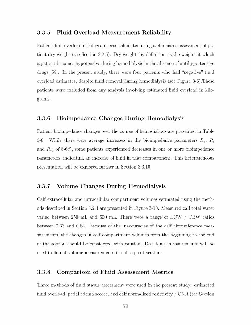
3.3.5 Fluid Overload Measurement Reliability
Patient fluid overload in kilograms was calculated using a clinician’s assessment of pa-
tient dry weight (see Section 3.2.5). Dry weight, by definition, is the weight at which
a patient becomes hypotensive during hemodialysis in the absence of antihypertensive
drugs [58]. In the present study, there were four patients who had “negative” fluid
overload estimates, despite fluid removal during hemodialysis (see Figure 3-6).These
patients were excluded from any analysis involving estimated fluid overload in kilo-
grams.
3.3.6 Bioimpedance Changes During Hemodialysis
Patient bioimpedance changes over the course of hemodialysis are presented in Table
3-6. While there were average increases in the bioimpedance parameters 𝑅𝑒, 𝑅𝑖
and 𝑅∞ of 5-6%, some patients experienced decreases in one or more bioimpedance
parameters, indicating an increase of fluid in that compartment. This heterogeneous
presentation will be explored further in Section 3.3.10.
3.3.7 Volume Changes During Hemodialysis
Calf extracellular and intracellular compartment volumes estimated using the meth-
ods described in Section 3.2.4 are presented in Figure 3-10. Measured calf total water
varied between 250 mL and 600 mL. There were a range of ECW / TBW ratios
between 0.33 and 0.84. Because of the inaccuracies of the calf circumference mea-
surements, the changes in calf compartment volumes from the beginning to the end
of the session should be considered with caution. Resistance measurements will be
used in lieu of volume measurements in subsequent sections.
3.3.8 Comparison of Fluid Assessment Metrics
Three methods of fluid status assessment were used in the present study: estimated
fluid overload, pedal edema scores, and calf normalized resistivity / CNR (see Section
79

Figure 3-10: Calf volume estimates calculated using bioimpedance data and calfcircumference measurements.
3.2.5). There was a weak correlation between clinician assessed fluid overload (ex-
pressed as % of body weight) and CNR (r = 0.50). Other researchers have observed
correlations between CNR and gold standard assessments of whole body ECW [42].
These results could be due to inaccurate clinical assessments of dry weight, or imply
that calf edema does not correlate with overall fluid status. A lack of correlation
between clinician assessed FO and CNR would not be entirely surprising, as fluid
buildup in the calf vs. rest of the body likely depends on a variety of factors such as
posture, etiology of a patient’s fluid overload, and individual patient factors.
There was a strong correlation between pedal edema scores and CNR (r = -0.75).
Pedal edema scores at higher CNR tend to be either one or zero, and increase as
CNR lowers (see Figure 3-11). There can be 10% changes in body weight without
perceptible changes in edema, which could explain the variable pedal edema scores
at higher CNR [59].
3.3.9 Changes in Total Calf Water
Patients with the highest ultrafiltration rates (8 mL/h/kg and above) tended to have
the largest changes in 𝑅∞, with patients with lower ultrafiltration rates having a
80
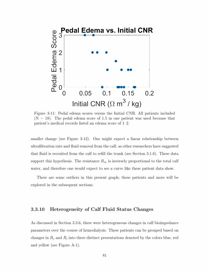
Figure 3-11: Pedal edema scores versus the Initial CNR. All patients included(N = 18). The pedal edema score of 1.5 in one patient was used because thatpatient’s medical records listed an edema score of 1–2.
smaller change (see Figure 3-12). One might expect a linear relationship between
ultrafiltration rate and fluid removal from the calf, as other researchers have suggested
that fluid is recruited from the calf to refill the trunk (see Section 3.1.6). These data
support this hypothesis. The resistance 𝑅∞ is inversely proportional to the total calf
water, and therefore one would expect to see a curve like these patient data show.
There are some outliers in this present graph; these patients and more will be
explored in the subsequent sections.
3.3.10 Heterogeneity of Calf Fluid Status Changes
As discussed in Section 3.3.6, there were heterogeneous changes in calf bioimpedance
parameters over the course of hemodialysis. These patients can be grouped based on
changes in 𝑅𝑒 and 𝑅𝑖 into three distinct presentations denoted by the colors blue, red
and yellow (see Figure A-1).
81
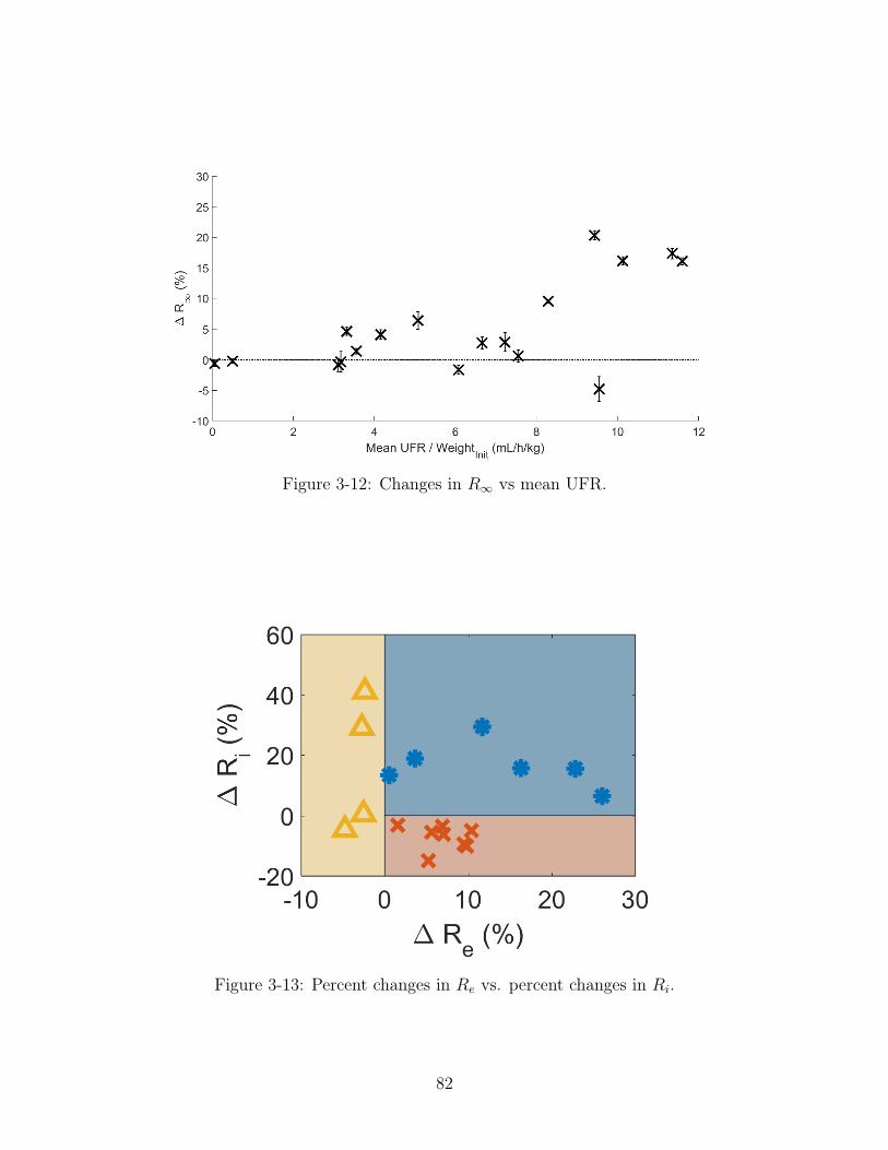
Figure 3-12: Changes in 𝑅∞ vs mean UFR.
Figure 3-13: Percent changes in 𝑅𝑒 vs. percent changes in 𝑅𝑖.
82

Blue patients
Patients in the blue group had increases in 𝑅𝑒 and 𝑅𝑖, which implies fluid removal
from both cECW and cICW. They had initial cECW/cTW ratios of 0.48±0.07, which
suggests moderate calf edema (an ECW/TBW ratio of 0.33 is considered normal [60]).
Figure 3-14a provides a visual representation of the fluid status changes. Blue patients
present as one might expect during standard hemodialysis: as fluid is removed from
plasma, it is partially refilled by the interstitial space, which in turn is partially refilled
by the intracellular space. This results in a decrease in both cECW and cICW.
Red patients
Patients in the red group have increases in 𝑅𝑒, but decreases in 𝑅𝑖, implying a shift
of fluid from cECW to cICW. They had initial cECW/cTW ratios of 0.48 ± 0.11,
which suggests moderate calf edema that was not statistically different from patients
in the blue group (p = 0.96). Figure 3-14b provides a visual representation of the
fluid status changes. Half the red patients also had an increase in 𝑅∞, implying
that cECW was moved both to cICW and out of the calf. Red patients tended to
have lower ultrafiltration rates than blue patients, but similar CNR in addition to
cECW/cTBW ratios (for CNR data, see Figure 3-15).
Other researchers have shown that overall ICW can increase over the course
of hemodialysis, particularly in patients with low ultrafiltration rates or diffusive
hemodialysis (see Section 3.1.3) [60,61]. Additionally, simulations performed by Akc-
ahuseyin et al. suggest that these fluid shifts into cells tend to be more pronounced in
low perfusion areas like the legs [60]. These data corroborate these findings as there
were fluid shifts into cells at low ultrafiltration rates and fluid shifts out of cells at
higher ultrafiltration rates for patients with similar CNR values.
One exception to the ultrafiltration rate relationship was a blue patient that had a
much lower ultrafiltration rate and lower CNR than other blue patients; this patient’s
ultrafiltration rate was in the same range as the red patients (see Figure 3-15). It
is possible that in this patient, a lower ultrafiltration rate was required to “prevent”
83

(a) (b)
Figure 3-14: Representative changes in calf volume in the (a) blue and (b)red groups. Dashed lines represent the original compartment volumes beforehemodialysis.
shifts into cICW due to higher plasma refill rates due to fluid overload.
Yellow patients
Yellow patients all had decreases in 𝑅𝑒, which implies increases in cECW. They had
cECW/cTW ratios of 0.65 ± 0.13, which suggests high calf fluid overload that is
statistically significantly higher than patients in the blue group (p = 0.02) and in
the red group (p = 0.03). Figure 3-14b provides a visual representation of the fluid
status changes. Two patients had no net change in 𝑅𝑖 as represented in the figure
(see error bars in Figure 3-16b), and two patients had increases in 𝑅𝑖. This means
that while all patients had increases in cECW, in two cases this increase appears to
come from elsewhere in the body, and in the other two cases it appears to come from
cICW in addition to the body. Yellow patients were also characterized by lower CNR
compared with patients in other groups (see Figure 3-15b), although there were two
red patients and one blue patient that had similar fluid overload levels.
Increases in cECW with no change in cICW could be due to posture / gravity.
Changes in posture result in fluid shifts in extracellular fluid via plasma, with shifts
into and out of the interstitial spaces in different segments of the body [62]. When
sitting or standing, fluid pools in the legs, which reverses when lying in a supine
or “semi-supine” position (i.e. legs and buttocks at same level, torso supported by
84

(a) Changes in 𝑅𝑖 as a function of meanUFR.
(b) Changes in 𝑅𝑖 as a function of InitialCNR.
Figure 3-15: Changes in the intracellular resistor 𝑅𝑖 as a function of: a)meanUFR, and b) CNR.
pillows or bed frame).
The patients in this study were all in a “semi-supine” position. While it is generally
assumed that patients in the “semi-supine” position will experience fluid shifts from
the calf to the trunk, this is the opposite of what was observed here. One study did
find that there was fluid pooling in the leg in a subset of patients when those patients
sat up in bed during their hemodialysis session [63], which suggests that postural
changes that result in pooling in the leg are possible. However, the present study
did not monitor posture. Additionally, it is not clear whether increases in cECW due
to posture only happen with low CNR, or could happen with a patient with higher
CNR. Future research should examine the role of posture and calf hydration in fluid
accumulation in the calf during hemodialysis.
The last two patients had increases in cECW and decreases in cICW, which implies
fluid flow into the extracellular space from cells. One of these patients had net zero
cTW change, whereas the other patient had a decrease in cTW. These two patients
had the lowest CNR of all patients, with moderate/low UFR. Fluid flows out of
cells when the interstitial fluid has higher osmotic pressure, which in this case could
occur due to the dialysate sodium concentration gradient and/or plasma refill (see
Section 3.1.3). Sodium is the main solute that could pull fluid out of cells. This
85

(a)(b)
Figure 3-16: (b) Percent changes in 𝑅𝑒 vs. percent changes in 𝑅𝑖; (a) changes incalf volume in the yellow group. Dashed lines represent the original compartmentvolumes before hemodialysis.
would occur if the dialysate sodium concentration is higher than the plasma sodium
concentration. However, both patients had dialysate sodium concentrations lower
than equilibrium, which would imply flow into cells rather than out of them. Another
possibility is that interstitial osmolarity is increased due to high plasma refill rates
due to low CNR. Other researchers have documented increases in plasma volume at
the end of hemodialysis [64]. However, this effect was documented several hours after
hemodialysis, so further research is needed to determine the mechanism behind this
effect.
3.4 Chapter Summary
In this study, calf bioimpedance measurements from hemodialysis patients were recorded
before and after each session. Total fluid removal from the calf was related to the
mean ultrafiltration rate, with higher ultrafiltration rates resulting in larger changes
in total calf water.
Changes in calf extracellular and calf intracellular volumes were heterogeneous
and were grouped into three different categories. The first group of patients had
decreases in both calf extracellular and intracellular fluid. This was in line with what
86

was originally expected. The second group of patients had fluid shifts from the calf
intracellular space to the calf extracellular space. This appears to be due to low
ultrafiltration rates compared to the patients in the previous group. The final group
of patients had increases in calf extracellular fluid. These patients had the most fluid
overload in the calf.
These findings suggest that fluid from the calf is recruited more readily at higher
ultrafiltration rates for patients with low to moderate edema levels in the calf. Pa-
tients with high calf edema have less fluid recruitment, or even fluid increases, in the
calf. These findings are contrary to what one might expect from the literature, in
that patients with the most overload had the lowest fluid removal from the calf.
The ultrafiltration relationship here support the hypothesis that fluid from the calf
is recruited to replenish fluid lost in the trunk. Higher ultrafiltration rates mean more
fluid removed from the trunk, which in this study led to larger decreases in calf total
water. The dependence of fluid recruitment on calf edema supports the hypothesis
that regional blood flow may play a role in fluid changes in the calf. If fluid was
removed from everywhere at the same rate, one would not expect any increases in
calf fluid to occur, which is what was observed here.
Some caution must be taken when considering the fluid shifts into and out of cells
presented here. Because compartment volumes can take hours to equilibrate after
hemodialysis, measurements performed immediately after the hemodialysis session
may not be at equilibrium. It is therefore likely that some portion of the fluid shifts
into and out of cells observed here would not persist at equilibrium (see Section 3.1).
Additionally, changes in fluid conductivity could account for some fraction of the
measured bioimpedance changes (see Appendix A).
87

88

Chapter 4
Determining Ideal Calf Electrode
Placement to Measure Fluid Status
Changes
The aim of this chapter is to determine the ideal electrode placement at the calf to
measure changes in fluid status. Calf impedance measurements during hemodialysis
range from 10–70Ω and change by single digit Ω values in most patients over the course
of their sessions. Because these changes are small, it is important to place electrodes
on the calf in a way that will maximize the impedance change due to fluid status
changes. The purpose of this section is to 1) determine an ideal electrode placement
topology and spacing for fluid status measurements at the calf and 2) determine an
ideal electrode placement around the calf.
4.1 Topology Simulations
There are two main functional requirements for a successful electrode configuration:
to maximize resistance changes due to fluid overload, and to maximize uniformity of
current distribution in the tissue. Finite element simulations were performed using
commercial software (COMSOL) to evaluate these requirements.
89
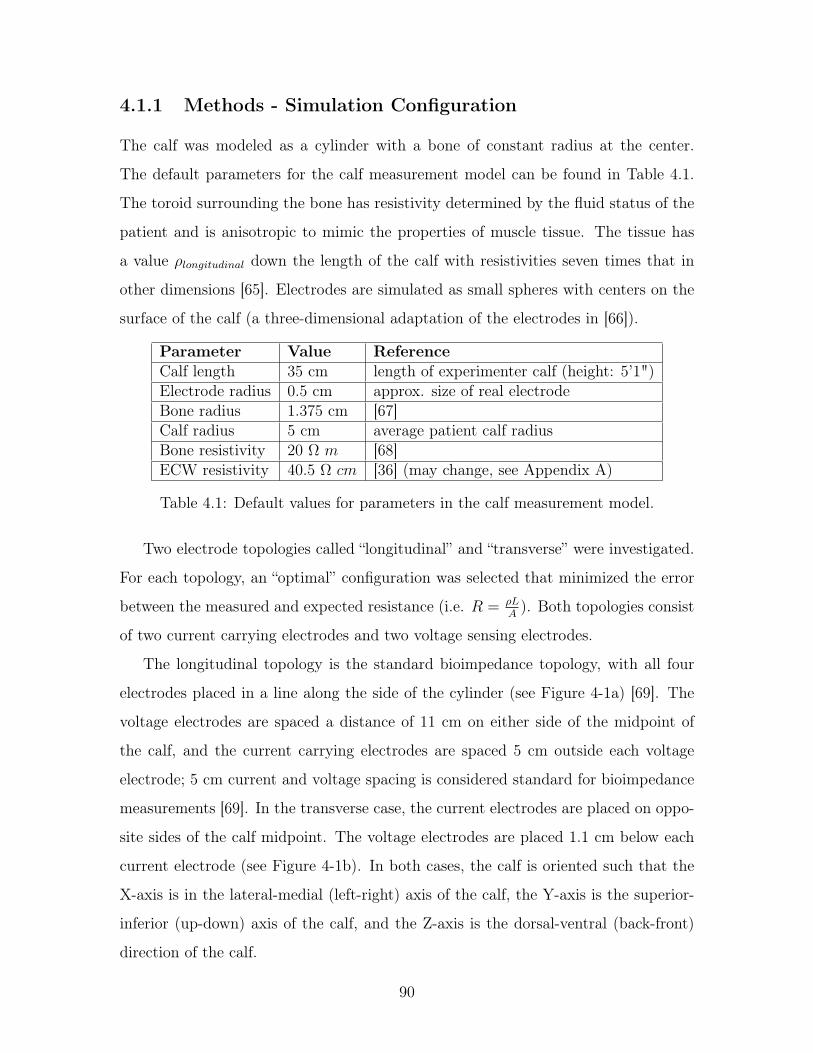
4.1.1 Methods - Simulation Configuration
The calf was modeled as a cylinder with a bone of constant radius at the center.
The default parameters for the calf measurement model can be found in Table 4.1.
The toroid surrounding the bone has resistivity determined by the fluid status of the
patient and is anisotropic to mimic the properties of muscle tissue. The tissue has
a value 𝜌𝑙𝑜𝑛𝑔𝑖𝑡𝑢𝑑𝑖𝑛𝑎𝑙 down the length of the calf with resistivities seven times that in
other dimensions [65]. Electrodes are simulated as small spheres with centers on the
surface of the calf (a three-dimensional adaptation of the electrodes in [66]).
Parameter Value ReferenceCalf length 35 cm length of experimenter calf (height: 5’1")Electrode radius 0.5 cm approx. size of real electrodeBone radius 1.375 cm [67]Calf radius 5 cm average patient calf radiusBone resistivity 20 Ω 𝑚 [68]ECW resistivity 40.5 Ω 𝑐𝑚 [36] (may change, see Appendix A)
Table 4.1: Default values for parameters in the calf measurement model.
Two electrode topologies called “longitudinal” and “transverse” were investigated.
For each topology, an “optimal” configuration was selected that minimized the error
between the measured and expected resistance (i.e. 𝑅 = 𝜌𝐿𝐴
). Both topologies consist
of two current carrying electrodes and two voltage sensing electrodes.
The longitudinal topology is the standard bioimpedance topology, with all four
electrodes placed in a line along the side of the cylinder (see Figure 4-1a) [69]. The
voltage electrodes are spaced a distance of 11 cm on either side of the midpoint of
the calf, and the current carrying electrodes are spaced 5 cm outside each voltage
electrode; 5 cm current and voltage spacing is considered standard for bioimpedance
measurements [69]. In the transverse case, the current electrodes are placed on oppo-
site sides of the calf midpoint. The voltage electrodes are placed 1.1 cm below each
current electrode (see Figure 4-1b). In both cases, the calf is oriented such that the
X-axis is in the lateral-medial (left-right) axis of the calf, the Y-axis is the superior-
inferior (up-down) axis of the calf, and the Z-axis is the dorsal-ventral (back-front)
direction of the calf.
90

(a) COMSOL model for the longitudinalelectrode configuration. The inner voltageelectrodes are spaced 22 cm apart and theouter current electrodes are 5 cm outsideeach voltage electrode.
(b) COMSOL model for the transverseelectrode configuration. The current elec-trodes are on on either side of the legsat the midpoint of the calf. The voltageelectrodes are 1.1 cm below the currentelectrodes.
Figure 4-1: The two electrode configurations used for simulations. The longi-tudinal configuration is shown in subfigure a and the transverse configuration isshown in subfigure b.
4.1.2 Methods - Fluid Overload
To simulate the tissue undergoing increasing fluid overload, it was assumed that in
the presence of edema, the length of the calf and the calf intracellular volume 𝑉𝑐𝐼𝐶𝑊
stay constant, and that increasing fluid in the calf causes an outward expansion of
the calf (i.e. increase in cross-sectional area). For an increase in edema ∆, the calf
volume 𝑉𝑐𝑎𝑙𝑓 and cECW volume 𝑉𝑐𝐸𝐶𝑊 change as:
𝑉𝑐𝑎𝑙𝑓,𝑛𝑒𝑤 = 𝑉𝑐𝑎𝑙𝑓,𝑜𝑟𝑖𝑔 + ∆ (4.1)
𝑉𝑐𝐸𝐶𝑊,𝑛𝑒𝑤 = 𝑉𝑐𝐸𝐶𝑊,𝑜𝑟𝑖𝑔 + ∆ (4.2)
As edema increases, the calf resistivity decreases. Recall that the apparent re-
sistivity 𝜌 (i.e. the 𝜌 used to calculate the resistance of the calf 𝑅 = 𝜌𝐿𝐴
) of tissue
91

is:
𝜌 =𝜌𝐸𝐶𝑊
(1 − 𝑐)3/2(4.3)
where 𝜌𝐸𝐶𝑊 is the resistivity of the extracellular fluid and 𝑐 is the volume fraction
of non-conducting tissue. In this case, 𝑐 = 1− 𝑉 𝑜𝑙𝑐𝐸𝐶𝑊
𝑉 𝑜𝑙𝑐𝑎𝑙𝑓, so the resistivity 𝜌 before and
after edema are:
𝜌𝑜𝑟𝑖𝑔 =𝜌𝐸𝐶𝑊𝑉 𝑜𝑙
3/2𝑐𝑎𝑙𝑓
𝑉 𝑜𝑙3/2𝑐𝐸𝐶𝑊
(4.4)
𝜌𝑛𝑒𝑤 =𝜌𝐸𝐶𝑊 (𝑉 𝑜𝑙𝑐𝑎𝑙𝑓 + ∆)3/2
(𝑉 𝑜𝑙𝑐𝐸𝐶𝑊 + ∆)3/2(4.5)
As both the volume of the cECW and the total volume of the calf increase at the
same rate, 𝜌 decreases. For the simulations, the initial radius of the calf was 5 cm,
and fluid was added or removed in increments of 1 cm of calf radius.
4.1.3 Methods - Current Uniformity
The second requirement to choose between the two electrode topologies is the unifor-
mity of current distribution in the tissue. This is important to ensure that current
penetrates into the tissue and as little preference is given to the surface of the skin
(which can be affected by non-fluid related parameters such as body temperature or
sweat) as possible.
Bioimpedance measurements performed in this thesis are four-point measure-
ments. Current is driven between two electrodes, and the resulting voltage is picked
up by a separate pair of electrodes. Both the distribution of driven current through
the tissue and the “pickup” of the voltage electrodes must be considered to determine
the uniformity of the measurement. Sensitivity is a measure of how much a volume
of tissue contributes to the overall measured resistance. The sensitivity 𝑆 is defined
92

as [66]:
𝑆 =𝐽𝑐𝑐𝐽𝑟𝑒𝑐𝑖
𝐼2(4.6)
where 𝐽𝑐𝑐 is the current density that results from a current 𝐼 driven between the
two current electrodes and 𝐽𝑟𝑒𝑐𝑖 is the current density that results from a current 𝐼
driven between the two voltage electrodes. The measured resistance 𝑅 for sensitivity
𝑆 is the integration in volume of the sensitivity times the resistivity:
𝑅 =
∫𝜌𝑆𝑑𝑣 =
∫𝜌𝐽𝑐𝑐𝐽𝑟𝑒𝑐𝑖
𝐼2𝑑𝑣 (4.7)
See Figure 4-2 for an example.
Current must be driven through both pairs of electrodes to calculate sensitivity.
One electrode of each pair is assigned to be a current source of 100𝜇𝐴 in COMSOL
and the other electrode is assigned to be ground. Then the sensitivity is calculated
as the normalized dot product of the resulting current densities in the calf. The
resistance is calculated as the integration of the sensitivity over the volume of the
calf, minus the space occupied by the electrodes. All simulations are performed at
DC, which corresponds to the low frequency bioimpedance case used to calculate
cECW.
To compare the two topologies, the sensitivity was analyzed at the midpoint of the
calf (𝐿𝑐𝑎𝑙𝑓/2) in both the X (left/right) direction and in the Z (front/back) direction.
The uniformity was calculated as the percent change between the maximum sensitivity
value in tissue and the minimum sensitivity value in tissue.
93

(a) Current density dis-tribution of the currentdriving electrodes (i.e.𝐽𝑐𝑐 in Equation 4.7).
(b) Current density dis-tribution of the voltagesensing electrodes (i.e.𝐽𝑟𝑒𝑐𝑖 in Equation 4.7).
(c) Sensitivity distribu-tion (log scale) that isthe dot product of sub-figures a and b, mul-tiplied by the resistiv-ity 𝜌 and normalized bythe squared current 𝐼2.
Figure 4-2: An example sensitivity distribution for a scenario with four electrodesplaced along the length of a rectangle. The current density of a constant currentdriven through the current electrodes (subfigure a) is multiplied by the currentdensity of a constant current driven through the voltage electrodes (subfigure b)to produce the sensitivity distribution in subfigure c.
94

Figure 4-3: The resistance changes as a result of changing fluid status (i.e. edema)for the longitudinal case (blue) and the transverse case (yellow).
4.1.4 Results
The longitudinal topology consistently had larger changes in resistance as a function
of edema (see Figure 4-3). For example, the change between 5 cm and 6 cm was
-36.7% in the longitudinal configuration and -16.0% in the transverse configuration.
There was poor sensitivity uniformity in both topologies. The best case in the X
direction was a change of -92% from the maximum sensitivity value in tissue to the
minimum value in the longitudinal configuration and -99% in the transverse configu-
ration (see Figure 4-4). The best case in the Z direction was -23% in the longitudinal
configuration and -87% in the transverse configuration (see Figure 4-5).
4.1.5 Discussion
The measured resistance in the longitudinal configuration changed about two times
more with edema than the transverse configuration (-36.7% vs. -16.0%). The absolute
change between the different configurations was less pronounced (−8.2 Ω vs. −6.0 Ω).
The larger percent change is due both to a larger starting resistance and a larger
absolute change in resistance.
Both configurations had poor sensitivity uniformity at maximum depth in the
95

(a) (b) (c)
Figure 4-4: A comparison of the longitudinal and transverse topologies in the XDirection (left to right) for Y = 𝐿𝑐𝑎𝑙𝑓/2 and 𝑍 = 0. (a:) graph of log sensitivityfor both topologies; (b:) Current distribution for the driving electrode pair forthe longitudinal topology; (c:) Current distribution for the driving electrode pairfor the transverse topology.
(a) (b) (c)
Figure 4-5: A comparison of the longitudinal and transverse topologies in the ZDirection (back-front) for Y = 𝐿𝑐𝑎𝑙𝑓/2 and 𝑋 = 0. (a:) graph of log sensitivityfor both topologies; (b:) Current distribution for the driving electrode pair forthe longitudinal topology; (c:) Current distribution for the driving electrode pairfor the transverse topology.
96

X-direction (-92% for longitudinal, -99% for transverse), with improvement in the
Z-direction for both configurations (-22.1% and -82.84% values, respectively). The
large decreases over the calf were due to both the anisotropy of the muscle tissue
(which causes current to prefer to flow down the leg rather than across it), and due
to the relatively short length of the calf. The calf length of 35 cm was chosen as a
conservative value, and the sensitivity should improve for longer calf lengths in the
longitudinal case (but will not affect the results in the transverse case).
Overall, the longitudinal configuration is more suitable for the impedance mea-
surement in hemodialysis than the transverse configuration. The measured resistance
changes more as cECW is added and the current is less concentrated in any one
particular region.
4.1.6 Improving Current Uniformity With Ring Electrodes
Placing electrodes in a longitudinal configuration increases expected changes in bio-
impedance during a simulated hemodialysis session. The main limitation of this
method is poor sensitivity uniformity due to the use of point electrodes.
One method to improve sensitivity is to use ring electrodes rather than point
electrodes. Previously, point electrodes were simulated as spheres with radii equal to
the electrode radius 𝑅𝑒𝑙𝑒𝑐. The center of each sphere was located on the calf surface.
If the electrodes are instead simulated as toroids with outer radii equal to the calf
radius 𝑅𝑐𝑎𝑙𝑓 and inner radii equal to the electrode radius 𝑅𝑒𝑙𝑒𝑐 (see Figure 4-6), the
sensitivity uniformity in both directions improves substantially to a change of -10%
in both the X-direction and the Z-direction compared with -92% and -23% in the
longitudinal configuration, respectively (see Figure 4-7).
Point electrodes are used for bioimpedance measurements primarily for conve-
nience. Ring electrodes can be more difficult to work with due to the need for gel
and adhesive around the whole leg. In patients with hair, it also means shaving more
of the leg. Ring electrodes should be more feasible to implement in the wearable
implementation using fabrics.
97

(a)(b)
Figure 4-6: (a) COMSOL model for the ring electrode configuration. The elec-trodes are spaced the same as in the longitudinal case, but with rings instead ofpoint electrodes. (b) A top down schematic view of a ring electrode. The lightestgray is calf muscle, the middle gray is bone, and the darkest gray is the electrode.The dashed line indicates the calf surface, with the ring electrode on either sideof it.
(a) (b)
Figure 4-7: (a) Comparison of sensitivity distribution in the longitudinal config-uration with and without the use of ring electrodes. (b) Current distribution forthe driving electrode pair in the longitudinal configuration using ring electrodes.
98

4.2 Placement Measurements
In this section, electrode placement is investigated through measurements with pa-
tients undergoing hemodialysis and COMSOL simulations.
4.2.1 Study Procedures - Electrode Placement
It was hypothesized that placing electrodes at the back of the calf instead of on
the side of the calf would result in higher impedance changes over the course of
hemodialysis. To evaluate this hypothesis, a variation of the protocol in Section 3.2.2
was implemented. Eight electrodes were placed on the body, with four in the same
locations as the previous protocol and four along the back of the calf. The electrodes
on the back of the calf were spaced the same as the four electrodes on the side and
at equivalent locations along the leg. Measurements with the side electrodes were
performed, followed by measurements with the back electrodes.
4.2.2 Results - Changes in 𝑅𝑒
Changes in 𝑅𝑒 between the beginning and end of the hemodialysis session for patients
enrolled in this part of the study is shown in Figure 4-8. There were larger changes
in 𝑅𝑒 in the back of the calf vs. the side of the calf in 4/7 patients. Of those patients
with larger changes at the back, two of those patients had a decrease in 𝑅𝑒 at the side
of the calf and an increase in 𝑅𝑒 at the back of the calf. The other two had increasing
𝑅𝑒 in both positions. One patient had equal changes in both locations, and the final
two patients had greater changes in the side of the calf than the back of the calf.
4.2.3 Results - Changes in 𝑅∞
Changes in 𝑅∞ between the beginning and end of the hemodialysis session for patients
enrolled in this part of the study is shown in Figure 4-9.There were larger changes
in 𝑅∞ in the back of the calf vs. the side of the calf in 5/7 patients. Two of those
patients had 𝑅∞ moving in opposite directions, with a decrease at the side and an
99

Figure 4-8: 𝑅𝑒 changes at the side and back of the calf over the course of thehemodialysis session.
increase at the back in patient 11, and an increase at the side and a decrease at the
back in patient 15. One patient had greater 𝑅∞ changes at the side of the leg, and
the last patient had about equal changes but in opposite directions (increase at the
side, decrease at the back).
4.2.4 Discussion
There appears to be a benefit in measuring at the back of the leg versus the side of
the leg in some patients, with higher impedance changes of up to 4% at the back
of the leg than at the side of the leg. However, in other patients there is a larger
change at the side of the leg. There were three patients that had bioimpedance
values move in different directions depending on the calf location. These patients
all had high calf fluid overload, and hence small calf bioimpedance values. It is not
known whether the difference in presentation at the side vs. back is a reflection of
a physiological difference in these patients or whether these differences are due to
systematic measurement error.
100

Figure 4-9: 𝑅∞ changes recorded at the side and back of the calf over the courseof the hemodialysis session.
4.3 Placement - Simulations
Heterogeneity in patient presentation has been observed when measuring bioimpedance
at the side and the back of the calf. COMSOL simulations were conducted to elu-
cidate the patterns observed. In particular, the effect of bone location and size on
impedance measurements and changes in impedance were investigated.
4.3.1 Methods
For these simulations, the calf was simulated as a cylinder with up to two bones
(the tibia and the fibula). Both bones were assumed to be cylinders with radii listed
in Table 4.3. Bone resistivity was assumed to be constant. Muscle resistivity was
set to the average calf resistivity calculated from all patients before and after the
hemodialysis session (see Table 4.2).
Voltage electrodes were placed in a longitudinal configuration (see Section 4.1)
spaced 10 cm apart. The current electrodes were spaced 5 cm from the voltage
electrodes. The location of the electrodes on the surface was moved along the cir-
cumference of the calf in 20 degree increments from 𝜃 = 0∘ to 𝜃 = 360∘, where 𝜃 = 0∘
is located on the calf as indicated in Figure 4-10.
101
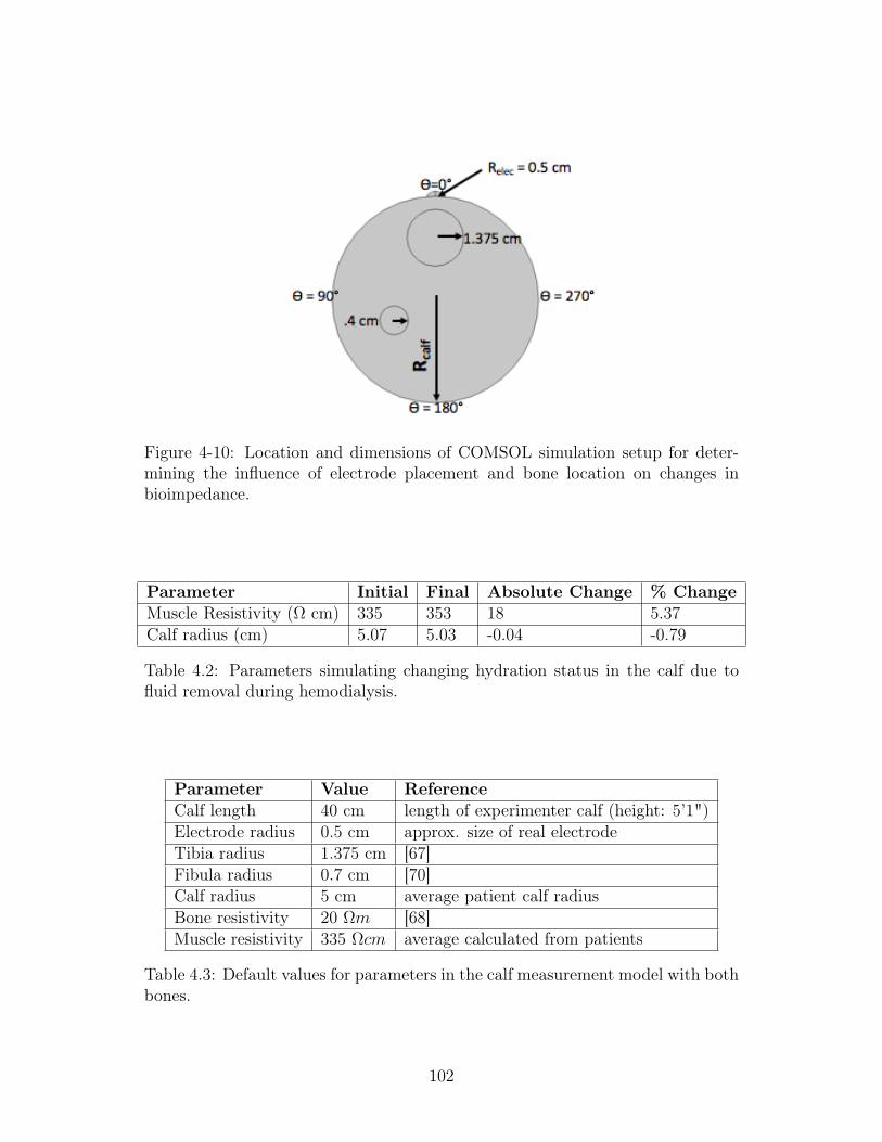
Figure 4-10: Location and dimensions of COMSOL simulation setup for deter-mining the influence of electrode placement and bone location on changes inbioimpedance.
Parameter Initial Final Absolute Change % ChangeMuscle Resistivity (Ω cm) 335 353 18 5.37Calf radius (cm) 5.07 5.03 -0.04 -0.79
Table 4.2: Parameters simulating changing hydration status in the calf due tofluid removal during hemodialysis.
Parameter Value ReferenceCalf length 40 cm length of experimenter calf (height: 5’1")Electrode radius 0.5 cm approx. size of real electrodeTibia radius 1.375 cm [67]Fibula radius 0.7 cm [70]Calf radius 5 cm average patient calf radiusBone resistivity 20 Ω𝑚 [68]Muscle resistivity 335 Ω𝑐𝑚 average calculated from patients
Table 4.3: Default values for parameters in the calf measurement model with bothbones.
102

Figure 4-11: Simulated resistance for different combinations of bones in the calf.
4.3.2 Results
Simulations for the calf with different combinations of bone/no bone are presented in
Figure 4-11. When no bones are present in the calf, the resistance is flat as a function
of 𝜃 with a resistance of 47 Ω. With the tibia only, the impedance peaks at 74 Ω at
𝜃 = 0∘ and the baseline resistance increases from 47 Ω in the no bone case to 50 Ω.
With the fibula only, the baseline resistance increases to 48 Ω with a peak of 51Ω
at 𝜃 = 120∘. With both bones, there are multiple peaks in resistance, with the tibia
peaking at 81 Ω at 𝜃 = 0∘ and the fibula peaking at 54 Ω at 𝜃 = 120∘.
Simulated changes in resistance due to simulated hemodialysis were consistently
around 7% across all theta (see Figure 4-12). The percent changes near the tibia
were slightly larger than those near the fibula (7.4% at 𝜃 = 0∘ vs. 6.9% at 𝜃 = 100∘),
and there was no difference between percent changes near the fibula and changes on
the opposite side of the leg (6.9% at 𝜃 = 100∘ vs. 6.9% at 𝜃 = 260∘). The changing
resistivity dominated the total resistance change, accounting for about 70% of the
total change in resistance.
103

Figure 4-12: Simulated change in resistance (%) in the simulated calf with twobones, including the total change and the change due to changing resistivity andradius independently.
4.3.3 Discussion
In this section, results from longitudinal measurements performed at the side of the
calf and at the back of the calf were presented. It was hypothesized that placement of
the electrodes in the back of the leg would result in higher changes in calf resistance
during hemodialysis because the back of the leg is further from the bones in the calf.
However, results from patients were mixed, with some patients having higher changes
at the back of the calf, and others having higher changes at the side.
Simulations were conducted to understand the influence of bone on the bio-
impedance measurement. Electrode placement was varied around the leg in 20∘ incre-
ments and the resistance was measured in a simulated before and after hemodialysis
state. There were higher absolute resistance values closer to calf bones than away
from them. Percent changes in calf resistance were consistent around the leg, with
only slightly larger changes (0.5% out of a total change of 7.5%) occurring near the
tibia. The changes in calf resistance were dominated by changing resistivity, which
accounted for 70% of the measured change, with area accounting for the other 30%.
There is a discrepancy between measured changes in bioimpedance during hemodial-
104

ysis, in which there were higher resistance changes at the back in some patients, and
the simulations, which suggest that there should be minimal influence of bone in gen-
eral, and the fibula in particular. The most likely explanation for these discrepancies
is that the resistivity of the calf is not uniform. This could be due to a number of
factors, such as resistivity differences in different muscle groups and fluid pooling in
different locations.
In practice, it is likely that the ideal electrode placement will depend on each
patient, with the ideal location somewhere between 90∘ and 270∘. Although there
were slightly larger percentage changes near the front of the leg, it is hypothesized that
these changes would be smaller when accounting for regional resistivity differences,
as more fluid is expected to pool in the back of the leg due to gravity.
4.4 Chapter Summary
In this Chapter, electrode topologies and placement for measurements of calf fluid
status via bioimpedance have been evaluated. Simulations were conducted to compare
the changes in resistance and the sensitivity in longitudinal and transverse topologies.
It was found that the longitudinal topology has greater changes in resistance due to
fluid status changes and improved current uniformity throughout the calf muscle
compared with the transverse topology. However, the current uniformity was limited
in both topologies. This can be substantially improved with ring electrodes in a
longitudinal topology using fabrics in the eventual wearable implementation.
Measurements were performed using the longitudinal topology and point elec-
trodes at the side and back of the leg. It was hypothesized that there would be
larger changes in the back of the leg than the side of the leg, but experimental results
were mixed. Simulations showed that when simulated with uniform resistivity in the
calf, there are larger changes in impedance near bone, not away from it. In practice,
ideal electrode placement will depend on that patient’s individual resistivity and fluid
distribution throughout the calf.
105

106

Chapter 5
Portable BIS System
This chapter will review the results of the final two thesis aims: to design and verify
a portable bioimpedance spectroscopy system on the bench (Thesis Aim 3) and in a
clinical setting (Thesis Aim 4).
5.1 Portable Bioimpedance System
A portable bioimpedance system that measures body impedance from 1 kHz to 1
MHz was designed and fabricated to the specifications shown in Table 5.1. It drives
an AC current of 100 𝜇𝐴 through two Ag/Ag-Cl electrodes placed on the body and
measures the resulting voltage between two neighboring Ag/Ag-Cl electrodes. The
device consists of the following components:
1. Custom-Designed Impedance Measurement PCB “Daughter Board”
2. ADI Bluetooth Low Energy (BTLE) and Microcontroller (MCU) PCB “Mother
Board”
3. Metal Enclosure
4. BNC cables w/ snap button attachments
Components 1 and 2 are mounted within a metal enclosure (Component 3). The
daughter board impedance measurement PCB (Component 1) is an analog front end
(AFE) designed by the author, and the mother board BTLE/MCU PCB (Component
2) is manufactured by Analog Devices. The device is connected to the Ag/Ag-Cl
107

Parameter Specification ActualFrequency range 1 kHz to 1 MHz 1 kHz to 1 MHz
Current 100𝜇𝐴𝑟𝑚𝑠 100𝜇𝐴𝑟𝑚𝑠
# Frequencies 10 / decade 10 / decadeMagnitude range 100 – 1000 Ω 35.1 – 3510Ω
Phase range 0 – -90∘ 0 – -90∘
Battery Life Several hours 4+ hrs
Table 5.1: Specifications for the portable bioimpedance spectroscopy system.
electrodes by BNC cables with snap-button connectors on the end (Component 4).
5.1.1 System Design
The Analog Front End drives current through the body and measures the resulting
voltage using the magnitude-ratio and phase-difference detection method (see Figure
5-2). A direct digital synthesizer (AD9833, ADI) is used to generate a sinusoidal
voltage that is converted to a sinusoidal current by an op-amp placed in the inverting
configuration (ADA4891, ADI). The resulting current is driven through the body by a
set of two electrodes. The current is in series with a known, non-inductive resistance
(350 Ω). The voltage across the body and the reference resistance are both amplified
by instrumentation amplifiers and converted to single-ended voltages (AD8231, ADI).
The resulting single ended voltages are then placed through a Gain-Phase Detector
(AD8302, ADI). The Gain-Phase Detector outputs a voltage proportional to the ratio
of the magnitudes and phase difference between the two signals. These two outputs
are sampled by two ADC input lines on the ADI mother board and sent to an iOS
device using Bluetooth Low Energy.
Power for the device is provided by a single-cell 3.7V Lithium-Ion battery with 600
mAH nominal charge capacity. A 3V analog and 3V digital supply are generated from
this voltage using an ADP3301-3 (ADI) voltage regulator for the analog supply and
a REF193 (ADI) voltage regulator for the digital supply. Power to the analog front
end and to the Bluetooth module can be toggled on and off by the microcontroller.
The voltages corresponding to the magnitude ratio and phase difference are sam-
pled by an ADC on the Analog Devices mother board. These data are then trans-
108

Figure 5-1: The portable bioimpedance spectroscopy measurement system insidethe enclosure.
mitted to a modified version of an Analog Devices iOS app. The iOS app visualizes
the magnitude and phase data and transmits them over Bluetooth Low Energy to an
MIT server using SFTP.
Four BNC cables with snap button attachments are used to connect the electrodes
to the participant (see Figure 5-3). The BNC cable shields are connected to battery
ground and the BNC conductor is connected directly to the electrode. Two different
electrode connectors were used during the experiments (see Figure 5-4). The custom-
designed electrode connectors were used during the first round of clinical testing. The
connectors were switched to using extensions of standard snap button connectors for
the second round of clinical testing due to concern for patient comfort when the
patient rested on the comparatively bulky connectors.
109

Figure 5-2: A schematic overview of the Magnitude-Ratio and Phase DifferenceDetection method. A fixed sinusoidal current is driven through the body and asense resistance. The voltage is amplified and measured by a Gain-Phase Detectorchip (AD8302).
5.1.2 Calibration
The system is calibrated with three RC networks using quadratic Lagrange interpo-
lation prior to each measurement session [71]. Each RC network is configured with
three circuit elements to mimic the electrical properties of the body (see Figure 5-5a).
Circuit parameters for each RC network are listed in Table 5-5b and a bode plot of
the calibration impedances can be found in Figure 5-6. All resistors in the RC net-
works had at least ± 1% tolerance and all capacitors had at least ± 10% tolerance.
Additionally, the impedance of each RC network was independently verified using an
Agilent 4294A precision impedance analyzer.
5.1.3 Data Processing
Data from the bioimpedance spectroscopy system are analyzed in MATLAB to ex-
tract circuit parameters according to the Cole model (see Section 2.2.2). MATLAB’s
lsqcurvefit algorithm was selected to achieve a non-linear least squares fit (see Section
3.2.3).
110

Figure 5-3: Electrode placement of the leg with one set of the electrode connectors.
5.2 Device Validation
A distinct set of four RC networks (Test 1 – 4 in Figure 5-5b) were used to validate the
experimental bioimpedance measurement system. For each network, bioimpedance
spectroscopy data from 1 kHz to 1 MHz was collected and the circuit parameters for
each model were extracted assuming a three element circuit model (see Sections 5.1.3
and 2.2.1). The percent error of the extracted parameters for each test RC network
is presented in Table 5.2. The error of the two resistances 𝑅𝑒 and 𝑅𝑖 were all less
than 1%, and the error for the capacitance 𝐶𝑚 was less than 3% with the exception
of Test 3, which was about 7%.
RC Network Re Error (%) Ri Error (%) Cm Error (%)Test 1 -0.02 -0.02 0.54Test 2 -0.11 0.37 2.7Test 3 0.56 -0.41 7.04Test 4 0.33 0.7 1.79
Table 5.2: The percent error of the experimental bioimpedance spectroscopy sys-tem measuring four different test RC networks (parameter values in Table 5-5b).
111

(a) The custom designed electrode con-nectors and the 3M-2560 Ag/Ag-Cl elec-trodes used during the first round of clin-ical testing.
(b) The re-purposed standard electrodeconnectors used during the second roundof clinical testing.
Figure 5-4: The two types of electrode connectors used during the hemodialysisstudies.
5.3 Device Repeatability
Human subjects testing with two healthy volunteers was performed to evaluate the re-
peatability of the bioimpedance spectroscopy system and compare BIS measurements
from opposite sides of the body. All testing took place at MIT’s Clinical Research
Center under the supervision of a trained nurse and informed consent was obtained
from all participants. After obtaining appropriate consent, 20 Ag/AgCl electrodes
(3M-2560) were placed in pairs on five different parts of both sides of the body. In
all cases, effort was made to place the electrodes in identical locations on both sides
of the body.
∙ Wrist/Hand: Two electrodes were placed on the palmar side of each arm (the
side with the palm of the hand on it). For each side, one electrode was at least 2
cm proximal from the process of the radial and ulna bones; the other electrode
was placed at least 5 cm proximal from the first electrode.
∙ Neck: Two electrodes were placed on the lateral sides of the neck and shoulder.
For each side, one electrode was placed on the lateral side of the neck 5-10 cm
below the hair line. The other electrode was placed superior to the clavicle,
112

(a) The three element circuitmodel used for the RC calibra-tion networks.
RC Network Re(Ω) Ri(Ω) Cm(nF)Calibration 1 60.4 12 70Calibration 2 316 1620 1.8Calibration 3 1000 953 2.2Test 1 402 402 5.6Test 2 464 499 2.3Test 3 300 300 2.7Test 4 60 100 11.2
(b) Values for each of the RC networks used forcalibration and testing.
Figure 5-5: The RC networks used to calibrate the system (topology in Figure5-5a) with component values in Figure 5-5b.
ideally at least 5 cm apart from the first electrode.
∙ Hips: Two electrodes were placed on the left and right side of the anterior side
of the trunk. For each side, one electrode was placed at least 5 cm superior to
the midpoint of the iliac crest. The other electrode was placed at least 5 cm
proximal from the first electrode.
∙ Knee: Two electrodes were placed on the anterior side around both knees. For
each side, one electrode was placed on the proximal side of the knee, at least 2
cm proximal to the patella (kneecap) and 2-5 cm lateral. The other electrode
was placed 2-5 cm distal and 2-5 cm lateral to the knee.
∙ Ankle/Foot: Two electrodes were placed on the medial surface of each leg. One
electrode was placed at least 2 cm proximal to the ankle. The other electrode
was placed at least 5 cm proximal from the first electrode.
After all the electrodes were placed on the participant, the participant laid down
on a hospital bed in the supine position for 5 minutes. After 5 minutes has elapsed,
the experimenter began taking bioimpedance measurements. Each frequency sweep
consists of 10 points per decade from 1 kHz to 1 MHz for a total of 31 points. Each
bioimpedance run consists of 5 continuous frequency sweeps, and runs are repeated
113

Figure 5-6: Bode plot of the RCs used to calibrate the experimental system.Component values are listed in Table 5-5b.
3 times per measurement type (see Figure 5-7). The BNC cables are removed and
replaced between measurements.
A total of 10 different types of measurements are made in the order shown below.
1. Hand (+) to foot (-) (left side)
2. Neck (+) to foot (-) (left side)
3. Hip (+) to foot (-) (left side)
4. Knee (+) to foot (-) (left side)
5. Hand (+) to foot (-) (right side)
6. Neck (+) to foot (-) (right side)
7. Hip (+) to foot (-) (right side)
8. Knee (+) to foot (-) (right side)
9. Foot (L/+) to foot (R/-)
10. Knee (L/+) to foot (R/-)
114

Figure 5-7: A schematic overview of repeatability measurements performed foreach measurement type. This method was repeated 10 times, once for each of thedifferent measurement types.
Repeatability is determined separately for magnitude and phase at each frequency
of interest. It is determined both “within run” (i.e. between the 5 different sweeps),
“across runs” (i.e. between the 3 different runs, which are each the average of 5
sweeps), and “across sides” (i.e. between the two different sides, if applicable). To
calculate the magnitude repeatability, the standard deviation of the measured mag-
nitude at the frequency of interest is calculated (this will be 5 points for “within run”
calculations and 3 points for “across run” calculations). The resulting standard devia-
tion is divided by the mean magnitude at that frequency and multiplied by 100. This
calculation is repeated for all frequencies, and the maximum (worst case) percent
error is reported. The repeatability calculation for the phase is the same, with the
exception that the absolute standard deviation is reported, not the percentage error.
Results for the two participants are shown in Figure 5.3. In BIS001, deviations
were smallest within runs and increased both across runs and across sides of the body.
BIS002 had a single run with high error (Neck to foot (left) 3) that skews the within
run results. Without this run the worst case within run repeatability was 2.45 % for
magnitude and 4.96∘ for phase. Error between runs was comparable between BIS001
and BIS002. Repeatability between sides was slightly higher between sides for BIS002
compared with BIS001.
115

Participant Within Runs B/W Runs Across SidesM (%) P (∘) M (%) P (∘) M (%) P (∘)
BIS001 2.65 1.42 3.09 1.48 5.01 4.94BIS002 10.57 7.15 3.18 4.93 6.94 6.41
Table 5.3: Standard Deviations of the worst case error within runs, across runs,and across sides. The worst case magnitude error is expressed in percentage pointsand the worst case phase error is expressed in degrees.
5.4 Comparing Commercial and Experimental Mea-
surement System
The experimental system has been verified on the bench (Thesis Aim 3). The final
aim is to verify the system in a clinical setting (Thesis Aim 4). Bioimpedance mea-
surements with patients undergoing hemodialysis were performed with a commercial
measurement system (Impedimed SFB7) and the experimental measurement system
described here. Measurements were performed with the same set of electrodes for each
system, with a configuration as shown in Figure 3-5. As described in Section 3.2, five
bioimpedance measurements were performed with the commercial system before and
after hemodialysis. In addition, continuous measurements were performed with the
experimental measurement system throughout the session. Five bioimpedance mea-
surements at the beginning and end of these continuous measurements were selected
for comparison with the commercial measurement system. To compare the two de-
vices, circuit parameters 𝑅𝑒 and 𝑅∞ were extracted from the bioimpedance spectra
using MATLAB (see Section 5.1.3).
5.4.1 Evaluation Criteria for Experimental System
The most important requirement for the experimental system is to be able to track
changes in bioimpedance consistently over an extended period of time. In this thesis,
the time period of evaluation is about 4 hours over the course of a hemodialysis
session. Bioimpedance measurements from the experimental system were compared
with measurements from a commercial measurement system. While the commercial
116

system may have errors of it’s own, for the sake of this work it is assumed to be the
“gold standard.”
The requirements for the experimental system in comparison with the commercial
measurement system are listed in Table 5.4. Because these measurements cannot be
readily compared with physiology, the specifications were selected based on the actual
impedance values and changes that need to be measured, namely impedances between
12 and 70 Ω with changes of single digit Ω values. The absolute difference specification
is present to evaluate the system’s ability to calculate absolute impedance values for
calculating the ECW/TBW ratio and calf resistivity (see Sections 2.4.2 and 2.4.4),
which depend on absolute bioimpedance values. The specification of 3 Ω represents
a much higher % error at low impedances than at high impedances. However, the
accuracy of calf bioimpedance at very low bioimpedances is less important as patients
with sufficiently low impedance values are almost certainly fluid overloaded.
Absolute differences between measurements do not include systematic error be-
tween systems. If, for example, there is a bias of 1 Ω between the two devices, this
will not count toward the absolute difference as it is a bias that can be calibrated out.
When relevant, Bland-Altman plots will be presented. A Bland-Altman plot is
commonly used in clinical testing to compare an experimental measurement with a
gold standard. In this case, this would be the experimental system and the commercial
measurement system. The measured data are plotted against each other on the
left side of the graph, with the unity line of Experimental = Commercial indicated
in dashed gray line and a solid line indicating the line of best fit based on linear
regression. Relevant equations and statistics are listed in the top left-hand corner of
the graph. The mean of the commercial and experimental systems is plotted on the X
access of the right side of each figure, with the difference Experimental - Commercial
presented on the Y-axis. In this case, the dashed black lines correspond to the limits of
agreement for the data set, which is defined as a 95% confidence interval or 1.96 times
the standard deviation of the points on the graph. The reproducibility coefficient
discussed in the text is 1.96 times the standard deviation.
117

5.4.2 Electrode Connectors
Two different electrode connectors were used for the measurements (see Figure 5-
4). The electrode connectors were switched after the first 10 patient runs both to
perform measurements at the back of the leg and because there were large absolute
differences in bioimpedance measurements between the two devices, particularly at
high frequencies after the run (see Figure 5-8). It was hypothesized that the electrode
connectors were contributing to loose electrode connections that were affecting mea-
surements with the experimental system. The electrodes were adjusted at the end of
the hemodialysis session and before performing measurements with the commercial
system, which appears to have artificially degraded the performance of the experi-
mental system. As such, graphs will present data with all or just the 7 patients with
new connectors as is relevant.
Specification ValueAbsolute difference between measurements ≤ 3 Ω
Difference in change ≤ 2 ΩDirection of change same direction (positive/negative)
Table 5.4: Specifications to compare the experimental measurement system withthe commercial measurement system.
5.4.3 Absolute Data
There were strong correlations between 𝑅𝑒 data as measured by the two devices (r =
1.00 before the hemodialysis session, r = 0.99 after the hemodialysis session). There
was an offset of 1.6 Ω between the two devices before the hemodialysis session and
1.2 Ω between the two devices after the hemodialysis session. The reproducibility
coefficients were 2.8 Ω and 4.3 Ω, respectively. Data from all but one patient was
within the limits of agreement (i.e. 1.96 SD) both before and after the session. The
repeatability coefficient of 𝑅𝑒 final data improved to 3.2 Ω after switching electrode
connectors.
𝑅𝑒 data from before the hemodialysis session satisfied the absolute difference func-
tional requirement (i.e. difference ≤ 3 Ω) with the exception of a single patient (16/17
118

= 94%), who had the lowest bioimpedance values measured. Although there does not
appear to be consistently higher errors at lower resistance values, it is likely that this
difference is due to limitations of both measurement systems resolving impedances
below 20 Ω.
𝑅𝑒 data from after the hemodialysis session satisfied the absolute difference func-
tional requirement for 14/17 (82%) of patients. Values that did not satisfy the func-
tional requirement included 𝑅𝑒 data from the patient that did not satisfy the func-
tional requirement with data from before the hemodialysis as well. The other two
patients were patients measured before the switch to the new connectors.
There were greater differences between the two devices for 𝑅∞ compared with 𝑅𝑒.
The correlations between the two devices before and after the session were r=0.94
and r=0.46, respectively. 𝑅∞ was underestimated both before the session by 3.4 Ω
and after the session by 5.6 Ω. The reproducibility coefficients were 6.6 Ω and 13.4
Ω. Data from all but one patient after the dialysis session was within the limits of
agreement.
𝑅∞ can be more difficult to estimate because of poor electrode connection and/or
stray capacitance. This may explain why there was both greater variation and ab-
solute differences between measurements from the two devices (as compared with 𝑅𝑒
data) both before and after the session. The differences between the two devices after
the hemodialysis session were much greater than before the session. This is most
likely due to loose electrodes toward the end of the hemodialysis session. After the
first round of testing, the type of electrode connectors were switched and the final
measurements were taken after the electrodes had been adjusted. Data using only
these patients is much improved (compare Figures 5-8 and 5-9). The offset reduced
from 5.6 Ω to 2.1 Ω (p = 0.07), with a new reproducibility coefficient of 4.8 Ω (down
from 13.4 Ω).
𝑅∞ data before the hemodialysis session satisfied the absolute difference require-
ment with 13/17 patients (76%). Of those not satisfying the requirements, three
patients were measured before transitioning to the new electrode connectors. 𝑅∞
data after the hemodialysis session satisfied the absolute difference requirement with
119

10/17 (58 %) with both sets of electrode connectors and 5/7 (71 %) with only the
new electrode connectors.
Figure 5-8: 𝑅∞ Final Data: a Bland-Altman plot comparing measured 𝑅∞ dataacquired at the end of the dialysis session.
120

Figure 5-9: 𝑅∞ Final Data (second round of patients only): a Bland-Altman plot comparing measured 𝑅∞ data acquired at the end of the dialysissession for only the patients with the new electrode connectors and improvedprotocol.
121
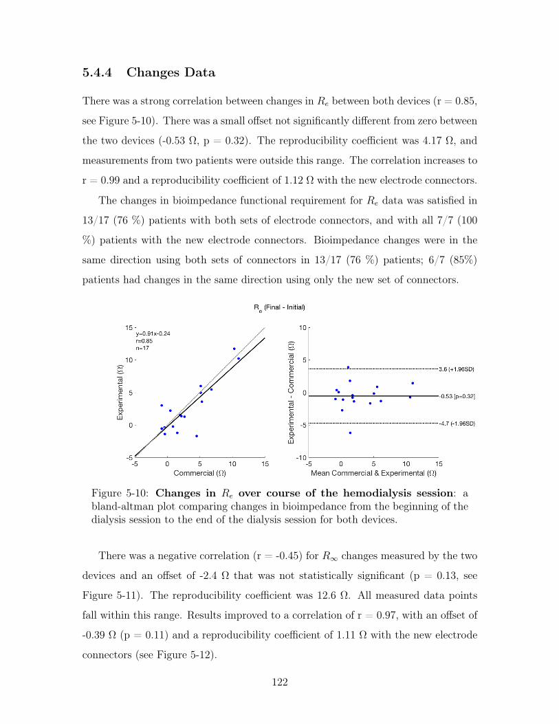
5.4.4 Changes Data
There was a strong correlation between changes in 𝑅𝑒 between both devices (r = 0.85,
see Figure 5-10). There was a small offset not significantly different from zero between
the two devices (-0.53 Ω, p = 0.32). The reproducibility coefficient was 4.17 Ω, and
measurements from two patients were outside this range. The correlation increases to
r = 0.99 and a reproducibility coefficient of 1.12 Ω with the new electrode connectors.
The changes in bioimpedance functional requirement for 𝑅𝑒 data was satisfied in
13/17 (76 %) patients with both sets of electrode connectors, and with all 7/7 (100
%) patients with the new electrode connectors. Bioimpedance changes were in the
same direction using both sets of connectors in 13/17 (76 %) patients; 6/7 (85%)
patients had changes in the same direction using only the new set of connectors.
Figure 5-10: Changes in 𝑅𝑒 over course of the hemodialysis session: abland-altman plot comparing changes in bioimpedance from the beginning of thedialysis session to the end of the dialysis session for both devices.
There was a negative correlation (r = -0.45) for 𝑅∞ changes measured by the two
devices and an offset of -2.4 Ω that was not statistically significant (p = 0.13, see
Figure 5-11). The reproducibility coefficient was 12.6 Ω. All measured data points
fall within this range. Results improved to a correlation of r = 0.97, with an offset of
-0.39 Ω (p = 0.11) and a reproducibility coefficient of 1.11 Ω with the new electrode
connectors (see Figure 5-12).
122

Changes in 𝑅∞ were within the functional requirement for 9/17 (53 %) patients
using both connectors, and for 7/7 patients (100 %) using the new connector. 7/17
(41 %) changes in 𝑅∞ were in the same direction using both sets of connectors; 4/7
(57 %) were in the same direction using the new connectors only. The changes in
𝑅∞ were small overall, which could explain why there are discrepancies between the
direction of changes even with the new connectors.
Figure 5-11: Changes in 𝑅∞ over course of the hemodialysis session: abland-altman plot comparing changes in bioimpedance from the beginning of thedialysis session to the end of the dialysis session for both devices.
Specification 𝑅𝑒 % Met 𝑅∞ % Met
Absolute difference between measurements (3 Ω) Initial: 94 (86)Final: 82 (86)
Initial: 76 (86)Final: 58 (71)
Difference in change (2 Ω) 76 (100) 53 (100)Direction of change (same) 76 (85) 41 (57)
Table 5.5: Percentage satisfaction of the functional requirements comparing theexperimental measurement system with the commercial measurement system.Each percentage is the total percentage (N = 17) with the percentage from usingthe new connectors only (N = 7).
123

Figure 5-12: Changes in 𝑅∞ over course of the hemodialysis session(second round of patients only): a bland-altman plot comparing changes inbioimpedance from the beginning of the dialysis session to the end of the dialysissession for both devices.
124

5.5 Chapter Summary
A portable bioimpedance spectroscopy system that measured bioimpedance in the
range of 1 kHz to 1 MHz was developed and verified both on the bench and in a
clinical setting (hemodialysis). Resistance and capacitance values extracted from
experimental system data were within 2% and 1.1 nF of the actual values, respec-
tively. The device repeatability for magnitude measurements was within 3% between
consecutive sweeps.
Calf bioimpedance measurements were performed before and after hemodialysis
patients using a commercial device and the experimental device developed in this
thesis. Ten patients were measured with a custom made electrode connector and the
final seven patients were measured using a standard button connector (see Figure
5-4). Functional requirements for such a comparison were presented in Table 5.4.
𝑅𝑒 absolute bioimpedance values and changes from beginning to end of hemodial-
ysis more closely satisfied the functional requirements than 𝑅∞ measurements. This
is not unexpected as stray capacitance and electrode contact disproportionately af-
fect 𝑅∞ measurements compared with 𝑅𝑒 measurements. The implementation of the
new electrode connectors improved the satisfaction of all functional requirements for
both measurement types both before and after the hemodialysis session. Because the
new connectors improved results both before and after, it’s likely that the connectors
themselves contributed to discrepancies between the measurements, in addition to
electrode contact issues at the end of the hemodialysis session. Ultimately, results
between the two devices were comparable, especially when the changes were greater
than 2 Ω.
125

126
Chapter 6
Conclusion
6.1 Summary of Contributions
This thesis had four aims:
1. Determine how changes in calf impedance are related to fluid removed during
hemodialysis
2. Determine the best electrode placement to perform the calf bioimpedance mea-
surement
3. Develop and verify a portable bioimpedance measurement system on the bench
4. Evaluate experimental system against a commercial system in a clinical setting
This work presents several contributions that addressed each of these aims:
1. A clinical test was conducted with 17 patients undergoing hemodialysis that
demonstrated that changes in the calf bioimpedance parameters 𝑅𝑒, 𝑅𝑖 and
𝑅∞ between the beginning and end of the hemodialysis session depend on calf
hydration and ultrafiltration rate (Thesis Aim 1).
2. Simulations were conducted that support using a longitudinal electrode topology
with ring electrodes for performing calf bioimpedance measurements (Thesis
Aim 2).
127

3. A clinical test was conducted with 7 patients undergoing hemodialysis that
demonstrated that changes in the calf bioimpedance parameter 𝑅𝑒 during hemodial-
ysis depends on electrode location along the calf (Thesis Aim 2).
4. A discrete, portable bioimpedance spectroscopy system was designed, built, and
verified on both the bench and in a clinical setting (Thesis Aims 3 and 4).
6.2 Progress Toward Wearable Bioimpedance Vision
and Future Work
The ultimate goal of this research project is to develop a wearable bioimpedance
measurement system to reduce heart failure readmissions in patients with Congestive
Heart Failure. This thesis focused on measuring calf bioimpedance in a controlled
environment (hemodialysis) and on improving the electrode placement for fluid status
monitoring. In this section, a summary of the findings of this thesis will be presented,
along with a discussion of how these results could be translated to an ambulatory CHF
setting and future work to achieve this vision.
6.2.1 Summary of Findings
Changes in the bioimpedance parameters 𝑅𝑒 and 𝑅∞ between the beginning of
hemodialysis and the end of hemodialysis were heterogeneous and categorized into
three distinct groups (see Section 3.3.6). There were two main findings relating to
different patient presentation: 1) that calf fluid overload affects changes in calf com-
partment volumes, and 2) that fluid flow in or out of cells is dependent on the mean
ultrafiltration rate in patients with lower calf fluid overload. In particular, patients
with lower fluid overload in the calf had fluid removal from the calf that was propor-
tional to the mean ultrafiltration rate. This was consistent with what was expected.
However, patients with higher fluid overload in the calf displayed greater heterogene-
ity, and a subset of these patients actually retained fluid in the calf despite a decrease
in Total Body Water.
128

Fluid shifts into or out of cells depended on the mean ultrafiltration rate for
patients with lower calf fluid overload. Fluid shifted out of cells at higher mean
ultrafiltration rates, and into cells at lower mean ultrafiltration rates. A portion of
these fluid shifts are transient and will not persist at equilibrium.
A combination of simulations and measurements were performed to determine the
ideal electrode placement for calf bioimpedance measurements. Simulation results
showed that measuring in a longitudinal topology (i.e. up and down the leg) resulted
in larger changes in calf bioimpedance and improved current uniformity compared
with measuring in a transverse topology (i.e. across the leg). Simulations also showed
that point electrodes have poor uniformity, but that that uniformity can be improved
almost ten times by using ring electrodes. Longitudinal measurements at the side
of the leg and the back of the leg revealed that electrode placement around the calf
depends on the individual patient. This is likely due to regional resistivity differences.
Measurements with ring electrodes would eliminate the need for evaluating the best
placement.
6.2.2 Translation to Ambulatory CHF
Findings from this thesis suggest that changes in calf bioimpedance will depend on
calf fluid overload and on the fluid removal rate (i.e. ultrafiltration rate). Patients
with high fluid overload had a heterogeneous and less predictable presentation than
those with lower levels of fluid overload. In an eventual ambulatory setting, patients
would have the wearable bioimpedance monitor placed when a clinician assesses a
patient to be at their “dry weight” (i.e. no fluid overload). This means that patients
should be at lower calf fluid overload levels, which had a more clear relationship
with changes in fluid status than patients with higher levels of fluid overload. Addi-
tionally, the wearable implementation will involve a feedback loop and intervention
to help minimize fluid overload in the calf. Should a patient reach sufficiently high
levels of fluid overload as observed in a subset of the hemodialysis patients, medical
intervention (i.e. hospitalization) would be necessary.
In a hemodialysis setting, fluid is removed rapidly from the body, resulting in
129
transient fluid shifts into and out of cells that do not persist at equilibrium. The rate
of fluid accumulation and removal in an ambulatory CHF setting will be an order of
magnitude slower than fluid accumulation/removal in hemodialysis (0 to 1 L / hour
in hemodialysis vs. 0 to 1 L / day in ambulatory CHF); this means that the system
should effectively be at equilibrium at all times and any changes in fluid status should
reflect longer lasting changes rather than transient ones.
Another consideration in translation to an ambulatory CHF setting is the expected
volume changes in that setting. In hemodialysis, patients have up to 0-4 kg of fluid
removed every other day. In ambulatory CHF, patients are instructed to consult a
physician when their weight increases by more than 2 kg over the course of a few
days. Because these changes are on the same order, the calf bioimpedance system
should be able to detect these changes so long as the device can consistently measure
bioimpedance over a period of several days. Ideally, the calf bioimpedance system
would measure bioimpedance over the period of a year without recalibration.
6.2.3 Future Work
Future work should integrate the measurements performed here in a wearable form
factor and determine the relationship between posture and fluid accumulation. In
particular, results from this thesis show that such a system should use ring electrodes
placed in a longitudinal configuration to perform calf bioimpedance measurements
from 1 kHz to 1 MHz. Using ring electrodes will ensure current uniformity throughout
the entire measurement volume and average out any regional resistivity differences in
the calf.
Additionally, future research should consider integration of strain gauges into the
wearable system. Strain gauges could allow for continuous assessment of calf cir-
cumference, which can be used for calf resistivity measurements (one metric of fluid
overload used in this thesis).
Fluid accumulation is affected by patient posture, so future research should con-
sider how different postures affect fluid accumulation in the calf. Accelerometers
could be integrated into the wearable system to enable correction for changes in pa-
130

tient posture.
131

Appendices
132

Appendix A
Conductivity Changes During
Hemodialysis
A.1 Motivation
Changes in bioimpedance were measured in patients in a hemodialysis unit. There
was a heterogeneous patient presentation in changes of the extracellular resistor 𝑅𝑒
and the intracellular resistor 𝑅𝑖 (see Figure A-1). These changes were presumed
to be due to fluid volume changes in the calf. However, there are other possible
explanations for these changes, such as a change in the extracellular conductivity.
This appendix will evaluate the possible influence of changes in fluid conductivity on
the measurements.
A.2 Relationship of Measured Resistance to Fluid
Conductivity
Assuming the calf is a cylinder, the measured low frequency resistance 𝑅𝑒 is a function
of the resistivity of the calf 𝜌 and the cross-sectional area 𝐴:
𝑅𝑒 =𝜌𝐿
𝐴(A.1)
133

Figure A-1: Percent changes in 𝑅𝑒 vs. percent changes in 𝑅𝑖.
Equation A.1 can also be expressed as a function of the calf volume 𝑉𝑐𝑎𝑙𝑓 :
𝑅𝑒 =𝜌𝐿
𝐴(A.2)
𝑅𝑒 =𝜌𝐿
𝐴* 𝐿
𝐿(A.3)
𝑅𝑒 =𝜌𝐿2
𝑉 𝑜𝑙𝑐𝑎𝑙𝑓(A.4)
If one assumes tissue is a conductive fluid with suspended non-conductive spherical
elements (i.e. cells), the resistivity 𝜌 is related to the volume fraction of the non-
conducting spheres 𝑐 and the resistivity of the conductive medium 𝜌𝐸𝐶𝑊 :
𝜌 =𝜌𝐸𝐶𝑊
(1 − 𝑐)3/2(A.5)
Assuming the non-conductive spheres have a volume equal to the total calf volume
𝑉 𝑜𝑙𝑐𝑎𝑙𝑓 minus the extracellular volume 𝑉 𝑜𝑙𝑐𝐸𝐶𝑊 , the volume fraction 𝑐 is:
𝑐 = 1 − 𝑉 𝑜𝑙𝑐𝐸𝐶𝑊
𝑉 𝑜𝑙𝑐𝑎𝑙𝑓(A.6)
134

The resistivity 𝜌 can then be expressed as:
𝜌 = 𝜌𝐸𝐶𝑊
(𝑉 𝑜𝑙𝑐𝑎𝑙𝑓𝑉 𝑜𝑙𝑐𝐸𝐶𝑊
)3/2
(A.7)
The equation for 𝑅𝑒 can then be expressed as:
𝑅𝑒 =𝜌𝐸𝐶𝑊
𝑉 𝑜𝑙𝑐𝑎𝑙𝑓𝑉 𝑜𝑙𝑐𝐸𝐶𝑊
3/2𝐿2
𝑉 𝑜𝑙𝑐𝑎𝑙𝑓(A.8)
𝑅𝑒 = 𝜌𝐸𝐶𝑊
√𝑉 𝑜𝑙𝑐𝑎𝑙𝑓𝑉 𝑜𝑙
3/2𝑐𝐸𝐶𝑊𝐿2 (A.9)
The conductivity of extracellular fluid 𝜎𝐸𝐶𝑊 is the inverse of the extracellular
resistivity 𝜌𝐸𝐶𝑊 , and so the final equation is:
𝑅𝑒 =
√𝑉 𝑜𝑙𝑐𝑎𝑙𝑓𝑉 𝑜𝑙
3/2𝑐𝐸𝐶𝑊𝐿2
𝜎𝐸𝐶𝑊
(A.10)
A.3 Determinants of Extracellular Conductivity
The extracellular conductivity is a function of the ionic content of the extracellular
fluid:
𝜎𝐸𝐶𝑊 =∑𝑖
= 𝜆𝑖𝑐𝑖 (A.11)
where 𝜆𝑖s are the ionic conductivities of extracellular solutes and 𝑐𝑖s are the con-
centration of those solutes. It is assumed that sodium is the dominant solute that will
dictate the conductivity, and any changes in conductivity are attributed to changes in
sodium concentration. The resistivity of extracellular fluid is assumed to be around
41 Ω𝑐𝑚 [37]. This translates to a conductivity of 0.02 𝑆/𝑐𝑚.
135
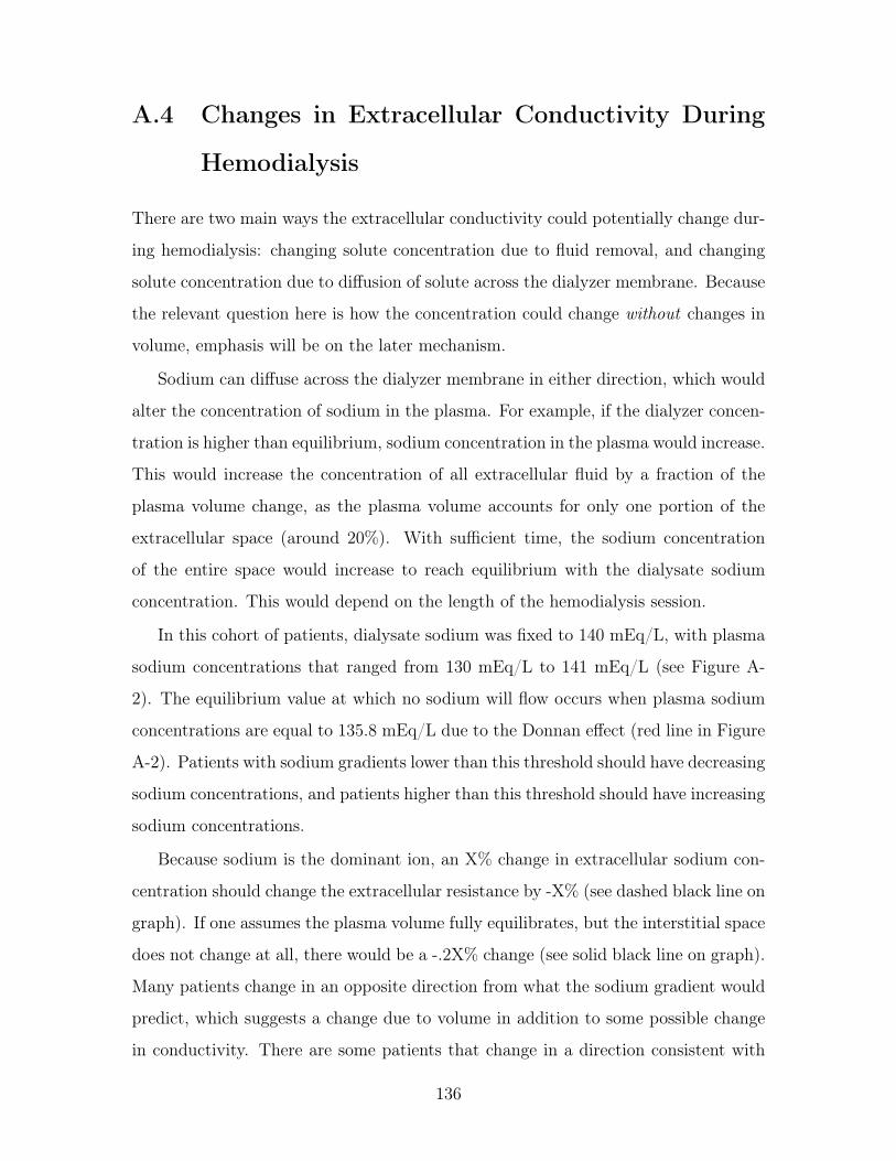
A.4 Changes in Extracellular Conductivity During
Hemodialysis
There are two main ways the extracellular conductivity could potentially change dur-
ing hemodialysis: changing solute concentration due to fluid removal, and changing
solute concentration due to diffusion of solute across the dialyzer membrane. Because
the relevant question here is how the concentration could change without changes in
volume, emphasis will be on the later mechanism.
Sodium can diffuse across the dialyzer membrane in either direction, which would
alter the concentration of sodium in the plasma. For example, if the dialyzer concen-
tration is higher than equilibrium, sodium concentration in the plasma would increase.
This would increase the concentration of all extracellular fluid by a fraction of the
plasma volume change, as the plasma volume accounts for only one portion of the
extracellular space (around 20%). With sufficient time, the sodium concentration
of the entire space would increase to reach equilibrium with the dialysate sodium
concentration. This would depend on the length of the hemodialysis session.
In this cohort of patients, dialysate sodium was fixed to 140 mEq/L, with plasma
sodium concentrations that ranged from 130 mEq/L to 141 mEq/L (see Figure A-
2). The equilibrium value at which no sodium will flow occurs when plasma sodium
concentrations are equal to 135.8 mEq/L due to the Donnan effect (red line in Figure
A-2). Patients with sodium gradients lower than this threshold should have decreasing
sodium concentrations, and patients higher than this threshold should have increasing
sodium concentrations.
Because sodium is the dominant ion, an X% change in extracellular sodium con-
centration should change the extracellular resistance by -X% (see dashed black line on
graph). If one assumes the plasma volume fully equilibrates, but the interstitial space
does not change at all, there would be a -.2X% change (see solid black line on graph).
Many patients change in an opposite direction from what the sodium gradient would
predict, which suggests a change due to volume in addition to some possible change
in conductivity. There are some patients that change in a direction consistent with
136

Figure A-2: Percent changes in 𝑅𝑒 as a function of ∆𝑁𝑎+ (Dialysate Sodium -Serum Sodium). The red line represents the equilibrium difference due to theDonnan effect. The solid black line represents the expected change in resistancedue to changes in sodium conductivity when only the plasma equilibrates (as-sumed 20% of cECW). The dashed black line represents the expected change inresistance when the entire cECW equilibrates.
the sodium gradient. In all of these patients, the change in resistance exceeds the pre-
dicted change, even if the entire extracellular space has reached equilibrium. In two
patients, the difference is only slightly larger than the change predicted by plasma
equilibration. Therefore, it is reasonable to conclude that resistance changes mea-
sured over the course of hemodialysis are a combination of conductivity and volume
changes, as conductivity alone cannot explain the measured changes in resistance.
A.5 Conclusion
Changes in calf bioimpedance were heterogeneous. It was hypothesized that these
differences were due to different changes in calf compartment volumes. This assump-
tion did not consider the possible effect of changing extracellular conductivity on the
137

measurements. Here it was shown that the changes measured during hemodialysis
exceed that which would be expected to be due to changes in extracellular conduc-
tivity, supporting the previous hypothesis that these changes are due to changes in
volume status.
138

Chapter 7
Bibliography
[1] D. Mozaffarian, E. J. Benjamin, A. S. Go et al., “Heart Disease and Stroke
Statistics - 2016 Update A Report From the American Heart Association,”
Circulation, p. CIR.0000000000000350, Dec. 2015. [Online]. Available: http:
//circ.ahajournals.org/content/early/2015/12/16/CIR.0000000000000350
[2] P. A. Heidenreich, N. M. Albert, L. A. Allen et al., “Forecasting the Impact
of Heart Failure in the United States A Policy Statement From the American
Heart Association,” Circulation: Heart Failure, p. HHF.0b013e318291329a, Apr.
2013. [Online]. Available: http://circheartfailure.ahajournals.org/content/early/
2013/04/24/HHF.0b013e318291329a
[3] L. R. Loehr, W. D. Rosamond, P. P. Chang et al., “Heart Failure Incidence
and Survival (from the Atherosclerosis Risk in Communities Study),” The
American Journal of Cardiology, vol. 101, no. 7, pp. 1016–1022, Apr.
2008. [Online]. Available: http://www.sciencedirect.com/science/article/pii/
S0002914907023636
[4] V. L. Roger, “Epidemiology of Heart Failure,” Circulation Research,
vol. 113, no. 6, pp. 646–659, Aug. 2013. [Online]. Available: http:
//circres.ahajournals.org/content/113/6/646
139

[5] C. W. Yancy, M. Jessup, B. Bozkurt et al., “2013 ACCF/AHA Guideline for the
Management of Heart Failure A Report of the American College of Cardiology
Foundation/American Heart Association Task Force on Practice Guidelines,”
Circulation, vol. 128, no. 16, pp. e240–e327, Oct. 2013. [Online]. Available:
http://circ.ahajournals.org/content/128/16/e240
[6] S. A. Hunt, W. T. Abraham, M. H. Chin et al., “2009 Focused Update
Incorporated Into the ACC/AHA 2005 Guidelines for the Diagnosis and
Management of Heart Failure in Adults A Report of the American College
of Cardiology Foundation/American Heart Association Task Force on Practice
Guidelines: Developed in Collaboration With the International Society for
Heart and Lung Transplantation,” Circulation, vol. 119, no. 14, pp. e391–e479,
Apr. 2009. [Online]. Available: http://circ.ahajournals.org/content/119/14/e391
[7] M. Dolgin, Nomenclature and Criteria for Diagnosis of Diseases of the Heart
and Great Vessels, 9th ed. Boston: Little Brown & Co, Mar. 1994.
[8] P. B. Adamson, “Pathophysiology of the transition from chronic compensated
and acute decompensated heart failure: New insights from continuous monitoring
devices,” Current Heart Failure Reports, vol. 6, no. 4, pp. 287–292, Dec. 2009.
[Online]. Available: http://link.springer.com/article/10.1007/s11897-009-0039-z
[9] M. R. Zile, T. D. Bennett, M. S. J. Sutton et al., “Transition From Chronic
Compensated to Acute Decompensated Heart Failure Pathophysiological
Insights Obtained From Continuous Monitoring of Intracardiac Pressures,”
Circulation, vol. 118, no. 14, pp. 1433–1441, Sep. 2008. [Online]. Available:
http://circ.ahajournals.org/content/118/14/1433
[10] C. Fantoni, S. Raffa, F. Regoli et al., “Cardiac Resynchronization Therapy
Improves Heart Rate Profile and Heart Rate Variability of Patients With
Moderate to Severe Heart Failure,” Journal of the American College of
Cardiology, vol. 46, no. 10, pp. 1875–1882, Nov. 2005. [Online]. Available:
http://www.sciencedirect.com/science/article/pii/S073510970501990X
140

[11] C.-M. Yu, L. Wang, E. Chau et al., “Intrathoracic Impedance Monitoring in
Patients With Heart Failure Correlation With Fluid Status and Feasibility of
Early Warning Preceding Hospitalization,” Circulation, vol. 112, no. 6, pp.
841–848, Aug. 2005. [Online]. Available: http://circ.ahajournals.org/content/
112/6/841
[12] K. F. Adams Jr., G. C. Fonarow, C. L. Emerman et al., “Characteristics
and outcomes of patients hospitalized for heart failure in the United States:
Rationale, design, and preliminary observations from the first 100,000 cases in the
Acute Decompensated Heart Failure National Registry (ADHERE),” American
Heart Journal, vol. 149, no. 2, pp. 209–216, Feb. 2005. [Online]. Available:
http://www.sciencedirect.com/science/article/pii/S0002870304004995
[13] W. T. Abraham, S. Compton, G. Haas et al., “Intrathoracic impedance vs daily
weight monitoring for predicting worsening heart failure events: results of the
Fluid Accumulation Status Trial (FAST),” Congestive Heart Failure (Greenwich,
Conn.), vol. 17, no. 2, pp. 51–55, Apr. 2011.
[14] mddiadmin, “FDA Panel Rejects Medtronic Remote Monitoring System,”
MDDI Online, Mar. 2007. [Online]. Available: http://www.mddionline.com/
article/fda-panel-rejects-medtronic-remote-monitoring-system
[15] hmpeditor, “Some Things We Just Can’t Have: The Demise of LAP-
TOP,” Jul. 2014. [Online]. Available: http://www.eplabdigest.com/articles/
Some-Things-We-Just-Can%E2%80%99t-Have-Demise-LAPTOP
[16] “FDA Okays Champion HF Monitoring System.” [Online]. Available: http:
//www.medscape.com/viewarticle/825805
[17] “No Coverage For CardioMEMS Decides Local Medicare Contractor |
MDDI Medical Device and Diagnostic Industry News Products and
Suppliers.” [Online]. Available: http://www.mddionline.com/blog/devicetalk/
no-coverage-cardiomems-decides-local-medicare-contractor-2-23-16
141

[18] X.-W. Yang, W. Hua, L.-G. Ding et al., “OptiVol fluid index predicts acute
decompensation of heart failure with a high rate of unexplained events,” Journal
of Geriatric Cardiology : JGC, vol. 10, no. 3, pp. 253–257, Sep. 2013. [Online].
Available: http://www.ncbi.nlm.nih.gov/pmc/articles/PMC3796699/
[19] D. J. v. Veldhuisen, F. Braunschweig, V. Conraads et al., “Intrathoracic
Impedance Monitoring, Audible Patient Alerts, and Outcome in Patients With
Heart Failure,” Circulation, vol. 124, no. 16, pp. 1719–1726, Oct. 2011. [Online].
Available: http://circ.ahajournals.org/content/124/16/1719
[20] V. M. Conraads, L. Tavazzi, M. Santini et al., “Sensitivity and positive
predictive value of implantable intrathoracic impedance monitoring as a
predictor of heart failure hospitalizations: the SENSE-HF trial,” European
Heart Journal, vol. 32, no. 18, pp. 2266–2273, Sep. 2011. [Online]. Available:
http://eurheartj.oxfordjournals.org/content/32/18/2266
[21] Medgadget, “Piix Wireless Home Cardiac Monitoring to Undergo Randomized
Trial,” Jun. 2009. [Online]. Available: http://www.medgadget.com/2009/06/
wireless_home_cardiac_monitoring_to_undergo_randomized_trials.html
[22] “toSense website.” [Online]. Available: http://www.tosense.com/
[23] I. S. Anand, W. H. W. Tang, B. H. Greenberg et al., “Design and performance
of a multisensor heart failure monitoring algorithm: results from the multisen-
sor monitoring in congestive heart failure (MUSIC) study,” Journal of Cardiac
Failure, vol. 18, no. 4, pp. 289–295, Apr. 2012.
[24] M. K. Shochat, A. Shotan, D. S. Blondheim et al., “Non-Invasive Lung
IMPEDANCE-Guided Preemptive Treatment in Chronic Heart Failure Patients:
a Randomized Controlled Trial (IMPEDANCE-HF Trial).” Journal of Cardiac
Failure, Apr. 2016. [Online]. Available: http://www.sciencedirect.com/science/
article/pii/S1071916416300082
142

[25] L. Beckmann, A. Cordes, E. Saygili et al., “Monitoring of body fluid in
patients with chronic heart failure using Bioimpedance - Spectroscopy,” in
World Congress on Medical Physics and Biomedical Engineering, September 7
- 12, 2009, Munich, Germany, ser. IFMBE Proceedings, O. Dössel and W. C.
Schlegel, Eds. Springer Berlin Heidelberg, 2009, no. 25/7, pp. 532–535. [Online].
Available: http://link.springer.com/chapter/10.1007/978-3-642-03885-3_148
[26] F. Zhu, M. K. Kuhlmann, P. Kotanko et al., “A method for the estimation
of hydration state during hemodialysis using a calf bioimpedance technique,”
Physiological Measurement, vol. 29, no. 6, pp. S503–516, Jun. 2008.
[27] T. Schlebusch, L. Röthlingshöfer, S. Kim et al., “On the Road to a Textile Inte-
grated Bioimpedance Early Warning System for Lung Edema,” in 2010 Interna-
tional Conference on Body Sensor Networks (BSN), Jun. 2010, pp. 302–307.
[28] J. Ramos, J. L. Ausin, G. Torelli, and J. F. Duque-Carrillo, “BioBee:
A Wireless Bioelectrical Impedance Monitoring System.” [Online]. Available:
http://dcis2009.unizar.es/FILES/CR2/p31.pdf
[29] M. Shochat, G. Charach, S. Meyler et al., “Prediction of cardiogenic
pulmonary edema onset by monitoring right lung impedance,” Intensive Care
Medicine, vol. 32, no. 8, pp. 1214–1221, Aug. 2006. [Online]. Available:
http://link.springer.com/article/10.1007/s00134-006-0237-z
[30] H. C. Lukaski, “Evolution of bioimpedance: a circuitous journey from
estimation of physiological function to assessment of body composition
and a return to clinical research,” European Journal of Clinical Nutrition,
vol. 67, no. S1, pp. S2–S9, Jan. 2013. [Online]. Available: http:
//www.nature.com/ejcn/journal/v67/n1s/full/ejcn2012149a.html
[31] S. Weyer, L. Röthlingshöfer, M. Walter, and S. Leonhardt, “Evaluation of
Bioelectrical Impedance Spectroscopy for the Assessment of Extracellular Body
Water,” Acta Polytechnica, vol. 52, no. 5, Jan. 2012. [Online]. Available:
https://ojs.cvut.cz/ojs/index.php/ap/article/view/1660
143

[32] K. S. Cole, “Permeability and Impermeability of Cell Membranes for Ions,” Cold
Spring Harbor Symposia on Quantitative Biology, vol. 8, pp. 110–122, Jan. 1940.
[Online]. Available: http://symposium.cshlp.org/content/8/110
[33] K. R. Foster and H. P. Schwan, “Dielectric properties of tissues and biological
materials: a critical review,” Critical Reviews in Biomedical Engineering, vol. 17,
no. 1, pp. 25–104, 1989.
[34] A. Ivorra, M. Genescà, A. Sola et al., “Bioimpedance dispersion width as a
parameter to monitor living tissues,” Physiological Measurement, vol. 26, no. 2, p.
S165, 2005. [Online]. Available: http://stacks.iop.org/0967-3334/26/i=2/a=016
[35] A. D. Lorenzo, A. Andreoli, J. Matthie, and P. Withers, “Predicting body cell
mass with bioimpedance by using theoretical methods: a technological review,”
Journal of Applied Physiology, vol. 82, no. 5, pp. 1542–1558, May 1997. [Online].
Available: http://jap.physiology.org/content/82/5/1542
[36] M. Y. Jaffrin and H. Morel, “Body fluid volumes measurements by impedance:
A review of bioimpedance spectroscopy (BIS) and bioimpedance analysis (BIA)
methods,” Medical Engineering & Physics, vol. 30, no. 10, pp. 1257–1269,
Dec. 2008. [Online]. Available: http://www.sciencedirect.com/science/article/
pii/S1350453308001100
[37] R. Buendia, F. Seoane, K. Lindecrantz et al., “Estimation of body fluids with
bioimpedance spectroscopy: state of the art methods and proposal of novel
methods,” Physiological Measurement, vol. 36, no. 10, p. 2171, 2015. [Online].
Available: http://stacks.iop.org/0967-3334/36/i=10/a=2171
[38] J. R. Matthie, “Second generation mixture theory equation for estimating
intracellular water using bioimpedance spectroscopy,” Journal of Applied
Physiology, vol. 99, no. 2, pp. 780–781, Aug. 2005. [Online]. Available:
http://jap.physiology.org/content/99/2/780
144

[39] S. R. Abbas, F. Zhu, and N. W. Levin, “Bioimpedance Can Solve Problems
of Fluid Overload,” Journal of Renal Nutrition, vol. 25, no. 2, pp. 234–237,
Mar. 2015. [Online]. Available: http://www.sciencedirect.com/science/article/
pii/S1051227614002118
[40] S. Grimnes and Ø. G. Martinsen, Bioimpedance & Bioelectricity Basics, 3rd ed.
Academic Press / Elsevier, 2015.
[41] G. Sergi, L. Lupoli, S. Volpato et al., “Body Fluid Distribution in Elderly
Subjects with Congestive Heart Failure,” Annals of Clinical & Laboratory
Science, vol. 34, no. 4, pp. 416–422, Oct. 2004. [Online]. Available:
http://www.annclinlabsci.org/content/34/4/416
[42] F. Zhu and N. W. Levin, “Estimation of Body Composition and
Normal Fluid Status Using a Calf Bioimpedance Technique,” Blood
Purification, vol. 39, no. 1-3, pp. 25–31, Jan. 2015. [Online]. Available:
http://www.karger.com/?doi=10.1159/000368937
[43] V. Wizemann, P. Wabel, P. Chamney et al., “The mortality risk of
overhydration in haemodialysis patients,” Nephrology Dialysis Transplantation,
vol. 24, no. 5, pp. 1574–1579, May 2009. [Online]. Available: http:
//ndt.oxfordjournals.org/content/24/5/1574
[44] U. Mulasi, A. J. Kuchnia, A. J. Cole, and C. P. Earthman, “Bioimpedance at
the bedside: current applications, limitations, and opportunities,” Nutrition in
Clinical Practice: Official Publication of the American Society for Parenteral and
Enteral Nutrition, vol. 30, no. 2, pp. 180–193, Apr. 2015.
[45] F. Zhu, S. Sarkar, C. Kaitwatcharachai et al., “Methods and reproducibility of
measurement of resistivity in the calf using regional bioimpedance analysis,”
Blood Purification, vol. 21, no. 1, pp. 131–136, 2003.
[46] “Dialysis,” Nov. 2017, page Version ID: 812966776. [Online]. Available:
https://en.wikipedia.org/w/index.php?title=Dialysis&oldid=812966776
145

[47] L. S. Costanzo, “Physiology - 4th Edition,” 2009. [Online]. Available:
https://www.elsevier.com/books/physiology/costanzo/978-1-4160-6216-5
[48] R. W. Schrier, Atlas of Diseases of the Kidney: Volume 5, volume 5 edition ed.,
W. M. Bennett and W. L. Henrich, Eds. Philadelphia: Wiley-Blackwell, May
1999.
[49] D. F. Keane, P. Baxter, E. Lindley et al., “The Body Composition Monitor: a
flexible tool for routine fluid management across the haemodialysis population,”
Biomedical Physics & Engineering Express, vol. 3, no. 3, p. 035017, 2017.
[Online]. Available: http://stacks.iop.org/2057-1976/3/i=3/a=035017
[50] T. Shulman, A. P. Heidenheim, C. Kianfar et al., “Preserving central blood vol-
ume: changes in body fluid compartments during hemodialysis,” ASAIO journal
(American Society for Artificial Internal Organs: 1992), vol. 47, no. 6, pp. 615–
618, Dec. 2001.
[51] F. Zhu, E. F. Leonard, and N. W. Levin, “Extracellular fluid redistribution dur-
ing hemodialysis: bioimpedance measurement and model,” Physiological Mea-
surement, vol. 29, no. 6, pp. S491–501, Jun. 2008.
[52] T. Chanchairujira and R. L. Mehta, “Assessing fluid change in hemodialysis:
Whole body versus sum of segmental bioimpedance spectroscopy,” Kidney
International, vol. 60, no. 6, pp. 2337–2342, Dec. 2001. [Online]. Available: http:
//www.kidney-international.theisn.org/article/S0085-2538(15)48127-X/fulltext
[53] S. R. Abbas, F. Zhu, G. A. Kaysen et al., “Effect of change in fluid distribution
in segments in hemodialysis patients at different ultrafiltration rates on accu-
racy of whole body bioimpedance measurement,” Journal of Applied Physiology
(Bethesda, Md.: 1985), vol. 116, no. 11, pp. 1382–1389, Jun. 2014.
[54] T. Hanai, “Theory of the dielectric dispersion due to the interfacial polarization
and its application to emulsions,” Kolloid-Zeitschrift, vol. 171, no. 1, pp.
146

23–31, Jul. 1960. [Online]. Available: https://link.springer.com/article/10.1007/
BF01520320
[55] F. Zhu, P. Kotanko, G. J. Handelman et al., “Estimation of normal hydration
in dialysis patients using whole body and calf bioimpedance analysis,”
Physiological Measurement, vol. 32, no. 7, p. 887, 2011. [Online]. Available:
http://stacks.iop.org/0967-3334/32/i=7/a=S12
[56] S. Eloot, “Experimental and Numerical Modeling of Dialysis,” Doctorate, Ghent
University. [Online]. Available: https://biblio.ugent.be/publication/468038/file/
1876450.pdf
[57] F. Zhu, E. F. Leonard, M. Carter, and N. W. Levin, “Continuous Measurement
of Calf Resistivity in Hemodialysis Patients using Bioimpedance Analysis,” in
2006 International Conference of the IEEE Engineering in Medicine and Biology
Society, Aug. 2006, pp. 5126–5128.
[58] B. Charra, “Fluid balance, dry weight, and blood pressure in dialysis,”
Hemodialysis International, vol. 11, no. 1, pp. 21–31, Jan. 2007. [Online].
Available: http://onlinelibrary.wiley.com/doi/10.1111/j.1542-4758.2007.00148.
x/abstract
[59] E. J. Mees, “Volaemia and blood pressure in renal failure: have old truths been
forgotten?” Nephrology, Dialysis, Transplantation: Official Publication of the
European Dialysis and Transplant Association - European Renal Association,
vol. 10, no. 8, pp. 1297–1298, 1995.
[60] E. Akcahuseyin, R. W. Nette, H. H. Vincent et al., “Simulation study of the in-
tercompartmental fluid shifts during hemodialysis,” ASAIO JOURNAL, vol. 46,
no. 1, pp. 81–94, Feb. 2000.
[61] S. Pastan and C. Colton, “Transcellular urea gradients cause minimal depletion
of extracellular volume during hemodialysis,” ASAIO transactions, vol. 35, no. 3,
pp. 247–250, Sep. 1989.
147

[62] G. Medrano, F. Eitner, A. H. Ismail et al., “Influence of body position,
food and beverage consumption on BIS measurements,” Journal of Physics:
Conference Series, vol. 224, no. 1, p. 012106, 2010. [Online]. Available:
http://stacks.iop.org/1742-6596/224/i=1/a=012106
[63] M. Fenech, M. Y. Jaffrin, and U. Malmen, “Reversibility of artifacts of fluid vol-
ume measurements by bioimpedance caused by position changes during dialysis,”
The International Journal of Artificial Organs, vol. 25, no. 3, pp. 217–222, Mar.
2002.
[64] H. A. Koomans, A. B. Geers, and E. J. Dorhout Mees, “Plasma volume recovery
after ultrafiltration in patients with chronic renal failure,” Kidney International,
vol. 26, no. 6, p. 848, Dec. 1984.
[65] B. R. Epstein and K. R. Foster, “Anisotropy in the dielectric properties of
skeletal muscle,” Medical and Biological Engineering and Computing, vol. 21,
no. 1, p. 51, Jan. 1983. [Online]. Available: https://link.springer.com/article/
10.1007/BF02446406
[66] Ø. Martinsen and S. Grimnes, “Some examples of electrode systems and their
sensitivity fields,” 2010. [Online]. Available: http://bioimpedance.bme.ufl.edu/
icebi/BioelectricityBasics.pdf
[67] A. Hrdlicka, “Study Of the Normal Tibia,” American Anthropologist,
vol. A11, no. 10, pp. 307–312, Oct. 1898. [Online]. Available: http:
//onlinelibrary.wiley.com/doi/10.1525/aa.1898.11.10.02a00010/abstract
[68] S. Gabriel, R. W. Lau, and C. Gabriel, “The dielectric properties of biological
tissues: II. Measurements in the frequency range 10 Hz to 20 GHz,” Physics
in Medicine and Biology, vol. 41, no. 11, p. 2251, 1996. [Online]. Available:
http://stacks.iop.org/0031-9155/41/i=11/a=002
148

[69] R. N. Baumgartner, W. C. Chumlea, and A. F. Roche, “Estimation of body com-
position from bioelectric impedance of body segments,” The American Journal
of Clinical Nutrition, vol. 50, no. 2, pp. 221–226, Aug. 1989.
[70] Y. Ide, S. Matsunaga, J. Harris et al., “Anatomical examination of the fibula:
digital imaging study for osseointegrated implant installation,” Journal of
Otolaryngology - Head & Neck Surgery, vol. 44, no. 1, Feb. 2015. [Online].
Available: https://www.ncbi.nlm.nih.gov/pmc/articles/PMC4349317/
[71] Y. Yang, J. Wang, G. Yu et al., “Design and preliminary evaluation
of a portable device for the measurement of bioimpedance spectroscopy,”
Physiological Measurement, vol. 27, no. 12, p. 1293, 2006. [Online]. Available:
http://stacks.iop.org/0967-3334/27/i=12/a=004
149