1

A new, high-resolution digital elevation model of Greenland fully validated with airborne laser altimeter data Jonathan L. Bamber Bristol Glaciology Centre, School of Geographical Sciences, University of Bristol, University Road, Bristol, BS8 1SS, UK, phone +44 117 928 8900, fax + 44 117 928 7878, email j.l.bamber@bris.ac.uk Simon Ekholm Kort & Matrikelstyelsen (National Survey and Cadastre), Rentemestervej 8, DK-2400 Copenhagen NV Denmark, phone +45-3587-5319, fax +45-3587-5052, William B. Krabill NASA/GSFC Wallops Flight Facility, Wallops Island, VA 23337, USA, phone + 1 804 824 1417, fax 1 804 824 1036 ABSTRACT A new digital elevation model of the Greenland ice sheet and surrounding rock outcrops has been produced at 1 km postings from a comprehensive suite of satellite remote sensing and cartographic data sets. Height data over the ice sheet were mainly from ERS-1 and Geosat radar altimetry. These data were corrected for a slope dependent bias that had been identified in a previous study. The radar altimetry was supplemented with stereo photogrammetric data sets, synthetic aperture radar interferometry, and digitised cartographic maps over regions of bare rock and where gaps in the satellite altimeter coverage existed. The data were interpolated onto a regular grid with a spacing of approximately one km. The accuracy of the resultant digital elevation model over the ice sheet was assessed using independent and spatially extensive measurements from an airborne laser altimeter that had an accuracy of between 10 and 12 cm. In a comparison with the laser altimetry, the digital elevation model was found to have a slope dependent accuracy ranging from –1.04±1.98 m to –0.06±14.33 m over the ice sheet for a slope range of 0.0-1.0°. The mean accuracy over the whole ice sheet was –0.33±6.97 m. Over the bare rock areas the accuracy ranged from 20-200 m, dependent on the data source available. The new digital elevation model was used as an input data set for a positive degree day model of ablation. The new elevation model was found to reduce ablation by only two percent compared with using an older, 2.5 km resolution model, which suggests that resolution-induced errors in estimating ablation are no longer important. 1. INTRODUCTION Digital Elevation Models (DEMs) are important in many geophysical applications and particularly so in glaciology. As a consequence, a number of models covering parts of the two ice sheets of Greenland and Antarctica have been published in recent years. Satellite radar altimeter (SRA) data from the GEOS-3 mission was first used to produce a DEM of the southern tip of Greenland [Brooks et al., 1978]. Seasat [Zwally et al., 1983] and Geosat [Zwally et al., 1987] SRA data were later used to produce DEMs covering the southern half of the ice sheet up to 72° N. It was not until the launch of ERS-1, in 1991, however, that coverage extended to almost the northern limit of Greenland enabling computation of a DEM of nearly the whole ice sheet [ Rapley et al., 1993, Ekholm, 1996]. In April 1994, ERS-1 was placed in its geodetic phase providing a single 336-day cycle giving across-track spacing at the southern tip of Greenland of 4 km. Data from this phase of the mission were used to produce a higher resolution (2.5 km) and accuracy DEM of the ice sheet [Bamber et al., 1997]. Here, we present a new DEM of the whole of Greenland, that has been improved in both resolution and accuracy, especially near the margins, by combining the ERS-1 geodetic-

2

phase data, described above, with a complementary suite of other satellite and airborne height data, and a new SRA bias correction scheme providing the most accurate, highest-resolution, and comprehensive DEM of the ice sheet and surrounding rock outcrops yet available. The accuracy of the ice-sheet-related part of the DEM was validated using independent measurements from a laser system known as the Airborne Topographic Mapper (ATM) [Krabill et al., 1995a]. The new DEM was used to recalculate surface runoff over the ice sheet and to examine short-wavelength features related to the ice dynamics and basal conditions. 2 DATA SETS SRA data from the geodetic phases of both ERS-1 and Geosat were used to provide maximum coverage over the ice sheet. Digital aerial photogrammetry and digitised topographic maps were used for the ice-free areas and also in some marginal regions where there were not sufficient SRA data. In this section, we provide a brief description of the various data sources employed. Figure 1 shows the coverage of all the data sources used in the generation of the DEM. 2.1 Satellite radar altimeter data SRA data from two different missions were used to provide good coverage over the whole of the ice sheet as explained below. 2.1.2 ERS data The dense track spacing of the Geodetic phase of ERS-1 and the improved tracking capability over ice has resulted in unprecedented coverage by SRA data of almost all of the ice sheet. The onboard SRA data recorder saved returned waveforms at 20 Hz, equivalent to an along-track ground separation of 335 m. The data were supplied by the U.K Processing and Archiving Facility (UK PAF) in a format known as the waveform product (WAP) and included 20 Hz waveforms and engineering and quality-control data. A large amount of auxiliary data were included in the WAP. Some of these data were used for quality assurance purposes, described in the appendix, and the rest were discarded. As a routine processing step the original orbits were replaced with more accurate ones provided by the Technical University of Delft (TUD), utilising the JGM-3 geopotential model [Tapley et al., 1996]. The orbits used here have a global accuracy of about 15 cm with higher accuracy in the northern hemisphere and lower in the southern [Scharroo and Visser, 1997]. Cross-over analysis over ocean areas surrounding Greenland had a RMS of 10 cm, which provides an upper limit to the regional orbit accuracy as these also include random errors due to uncertainties in the atmospheric corrections. 2.1.2 Geosat The ERS-1 geodetic phase data provide excellent coverage of the northern half of the ice sheet. At its southern limit, of about 60° N, however, the track spacing is about 4 km, limiting the across-track resolution of the data. To overcome this, Geosat Geodetic Mission data were used. They were provided by Goddard Space Flight Center (GSFC)/Hughes STX as part of NASA's Mission to Planet Earth Program [NASA, 1997], and were collected over a period of 18 months from 1985-'86. We used the Ice Data Record (IDR), which contains a number of instrument and geophysical corrections. The IDR is a geophysical product, unlike the WAP, which, consequently, required relatively little error checking and less manipulation to extract the fully corrected elevation. Details of the processing steps applied to this data set are presented in the appendix. Several orbits are available in the IDR product and we used those calculated using the JGM-3 gravity model, as for the ERS-1 data. 2.2 Laser Data

3

The laser altimeter data were acquired with a circular scanning system known as the Airborne Topographic Mapper (ATM) that collected dense 200-m-wide swaths of points [Krabill et al., 1995b]. The laser spot diameter on the surface was about 1 m, in contrast to the footprint of the altimeter, which can be as large as 20 km, and the laser data accuracy is generally of the order of 10 cm. The ATM data were compressed to averaged values at about 25 m intervals along the flight-line. Standard deviations in range for each averaged point proved useful for identifying occurrences of the laser "losing" the surface due to clouds, diamond dust or other atmospheric interference [Bamber et al., 1998]. Erroneous ATM data affected by atmospheric influences were removed from the comparison by excluding any averaged ATM point with a standard deviation greater than 1 m. The laser data were not used directly for incorporation into the final DEM but they served as a useful calibration of the satellite SRA (see sections 3.1 and 5). The coverage of ATM data is shown in Figure 2. 2.3 Photogrammetric and cartographic data Kort & Matrikelstyrelsen (KMS) and Geologiske Undersøgelser (GEUS, The Geological Survey of Denmark and Greenland) have, over several years, produced digital height data by photogrammetric analysis of aerial photos. KMS has produced coverage of all ice-free areas, and some ice-covered regions as well, north of 78° N. The photography was scanned along profiles with a separation of 220 m, which also defines the along-track resolution of the resultant topographic data. This analysis produced an easily manipulated data set of uniform coverage. The remaining digital photogrammetric data were obtained by GEUS in areas of particular geological interest. The GEUS data were extracted along contour lines at 100 m intervals. Previous analyses of these data suggest that they have an RMS error of about 20 m [Ekholm, 1996]. The U.S. National Imaging and Mapping Agency, NIMA, (formerly the Defense Mapping Agency) has generated digital elevation models at various resolutions and levels of accuracy, covering a substantial part of the earth. A large fraction of these are classified but a number of the finest resolution versions, called DTED level 0 products, have become available to the scientific community. These include three models that incorporate parts of the Greenland coast (south, central east and north-west, respectively) with a resolution of approximately 1 km. Preliminary examination indicates that the accuracy of the NIMA models is of the order of 50-75 m RMS which is significantly poorer than the products from GEUS and KMS and. A technique of importance for future topographic mapping of Greenland is synthetic aperture radar interferometry (InSAR). We have obtained some preliminary results using InSAR tandem data from ERS-1 and ERS-2 over Jameson Land on the central Greenland east coast (Figure 1). This data set, which was included in the computation of the new DEM, was produced with a horizontal resolution of 100 m and a vertical accuracy of 20 to 30 m, which is comparable to the photogrammetric data. On a considerable part of the coast, however, no reliable digital data exist and KMS has consequently manually digitised elevation information from paper maps. This digitising was performed using a fairly primitive technique with a variable resolution. Furthermore, the maps are of a highly variable quality. Contour lines on the margins of the ice sheet, in particular, are of dubious accuracy, and were included only if no other data existed. It is difficult to determine the mean error for these data but we estimate that it is not less than 100 m. 3 RADAR ALTIMETER DATA REDUCTION SRAs were designed, primarily, for operation over oceans. Over non-ocean surfaces a number of corrections need to be applied due to the undulating nature of the surface. The first of these

4

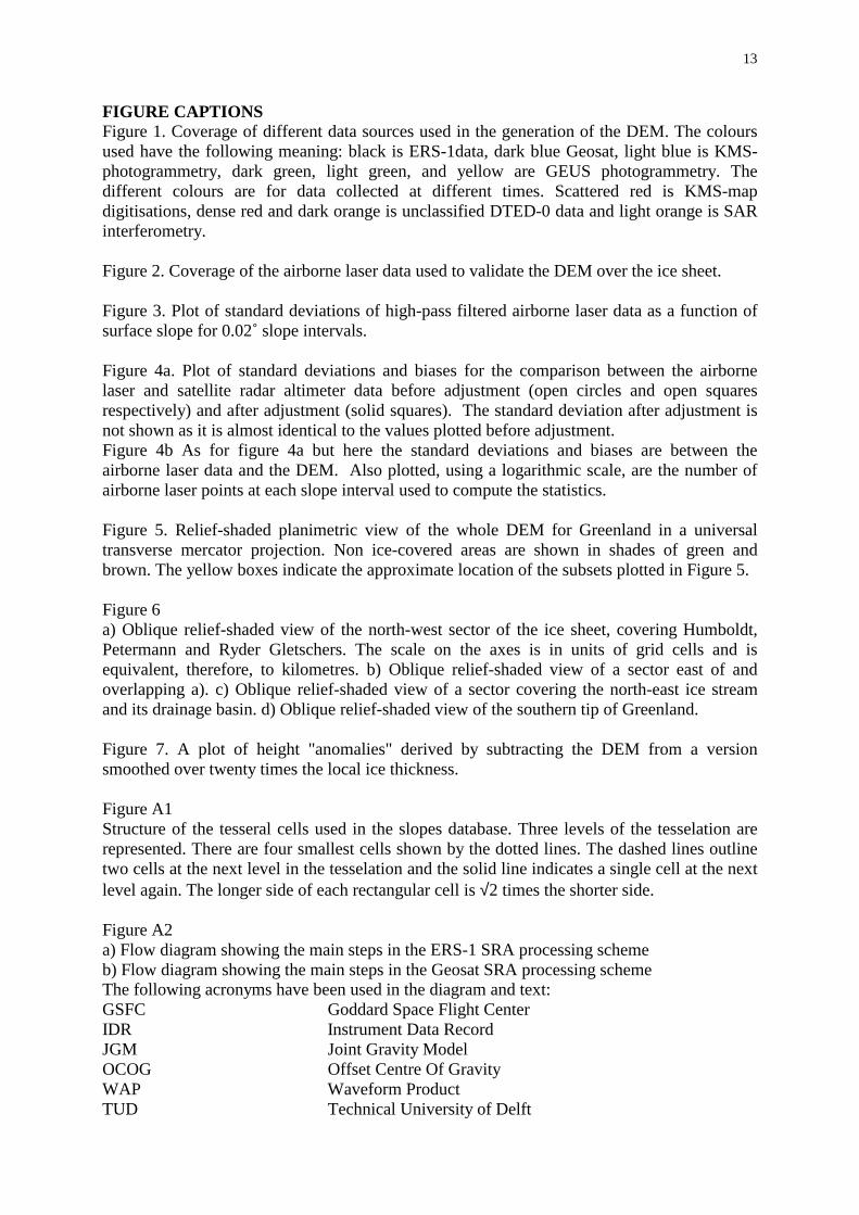
is a range-estimate refinement procedure known as waveform retracking. The second corrects for the slope-induced error that results from the fact that the altimeter ranges to the nearest point on the ground rather than the nadir point. Finally, various quality assurance tests are required due to the frequent "loss of lock" of the surface over undulating terrain and the tendency for the instrument to track noise in these cases [Scott et al., 1992]. The methodolo-gies employed to carry out these tasks can have an important impact on the accuracy of the results [Bamber, 1994]. The details are, however, of a technical nature and are, therefore, relegated to Appendix I. In this section we concentrate only on a procedure that is unique to this study and that relates to the removal of a bias that is inherent in the SRA data (for reasons explained below) even after the aforementioned corrections have been applied. 3.1 Adjustment for bias in radar altimetry. A consequence of using the relocation method for slope correction is that the corrected SRA points tend to cluster on local topographic peaks of the surface whereas the troughs are less well sampled (if at all) by the adjusted data. This is not an error, as it reflects the fact that these areas are indeed those that are ranged to by the SRA. It does, however, introduce a significant bias in the sampling of the surface. In order to determine the relationship between the local surface slope, α, and this bias, a comprehensive analysis of the ATM laser profiles was undertaken. The full details are given elsewhere [Ekholm et al. 2000] and, consequently, only the key points are presented here. The bias in the data is related to the average magnitude of the local undulations that have a wavelength less than the size of the beam limited footprint. To assess the distribution of this bias, the ATM profiles were high-pass filtered along-track using a filter with a cut-off wavelength of 30 km, corresponding roughly to the maximum size of the footprint. The high-pass filtered residuals were grouped in 0.02° intervals of slope, α. Means and standard deviations, σ, were computed for each group. The standard deviations calculated within each interval are taken as a measure of the mean amplitude of the undulations. Figure 3 shows the relationship between α and σ. For slopes of about 0.8° or less, a linear fit gives a correlation coefficient of 0.92 [Ekholm et al., 2000]. Above 0.8°, the relationship is less clear and there is more scatter in the data due, we believe, to the relatively poor areal distribution of ATM data for the higher slope intervals and the more noisy SRA-derived heights for slopes greater than the half-power beam-width of the instrument. A least squares fit to the data for slopes less than 0.8° gave the relation: σ = 12.0 α + 0.5 (1) The straight line in figure 3 represents this equation graphically. Equation 1 was used to correct the SRA data up to 0.8°. The local surface slope estimate at the sub-satellite point was used once its position had been corrected for the slope-induced error (see Appendix I). Above 0.8° a constant bias of 10.1 m was applied. There is no theoretical reason for expecting a linear relationship between α and σ and Figure 3 suggests that at higher slopes a linear fit may not be appropriate. The limited spatial extent of the higher slope data, however, made it impossible to determine reliably what kind of relationship existed for angles above 0.8°. Nonetheless, we found that employing this correction reduced the bias markedly for all slope intervals without increasing the standard deviations. After applying the correction the SRA data were compared with the observed ATM heights. Overall the bias and the standard deviation between the ATM and SRA data were reduced from 3.10 m to -0.68 m and from 7.15 m to 6.68 m, respectively. Implementing the bias correction reduced the correlation coefficient between the residual height differences and slope from 0.4 to less than 0.1. The effect on the bias and standard deviation is shown in figure 4a, plotted against surface slope.

5

It should be noted that the data for slopes above about 1° were obtained from around fifteen spatially extremely limited areas and cannot, therefore, be considered a statistically representative spatial sample of the surface. This is illustrated by the trend in the number of ATM points found within a particular slope interval, which is plotted in Figure 4b. 4 DEM GENERATION The distribution of the ice sheet data and the majority of the coastal data was consistent with a model with a horizontal resolution of approximately 1 km. To reduce the noise in the SRA data, they were averaged locally at this resolution. A least squares collocation technique with a second order Markov model defining the covariances between data and modeled elevation was used to generate the DEM from the data [Kasper, 1971]. This approach has been shown to be effective for elevation modeling as it takes into account variations in data accuracy in the determination of the weighting matrix so that the detail in the DEM reflects the local data quality [Ekholm, 1996]. The data used to estimate each modeled height were selected by defining a north-south and an east-west axis through each model point, and the 3 closest data points from each quadrant were then used. The model was generated as a grid in geographical polar co-ordinates with a spacing of 0.01° and 0.025° in latitude and longitude, respectively (corresponding to approximately 1 km). The true spatial resolution of the DEM (as opposed to the grid spacing) depends on the local data source, however. The stereo-photogrammetric and InSAR data have a resolution of better than 1 km (section 3.2). The SRA data, however, have a variable spatial resolution dependent on the roughness of the surface. For a specular surface the pulse-limited footprint of the ERS-1 SRA is about 2 km and this represents the best resolution using the processing methodology used here. In general, due to the spreading of the pulse by surface undulations the resolution will be somewhat poorer than that. An analysis of the covariance in SRA data from West Greenland suggested that height measurements were correlated at distances below about 4 km [Lingle et al., 1990]. The resolution of the SRA data lies, therefore, somewhere between these two limits. 5 VALIDATION OF THE NEW DEM This is presented in two parts based on surface type: the ice sheet and the ice-free regions. On the rock outcrops, there is a large set of reference points available. These data have been extracted from aerial photogrammetry. They have an RMS accuracy of about 10 m. A comparison with an earlier DEM of Greenland [Ekholm, 1996] indicated that the accuracy of the part computed from the aerial-photogrammetry was of the order of 25-30 m RMS. For the considerable part of the coast that is covered only by elevations extracted from maps, the error is much larger however (200-300 m RMS), and the model only provides the general long-wavelength topography of those regions. Figure 1 shows the coverage by different data sets and, therefore, the accuracy of the DEM in these regions. On the ice sheet the most accurate and extensive validation data set comprised the ATM measurements. It should be noted that these were used to estimate the bias in the SRA data (section 3.1) so the model and the control data are not entirely uncorrelated in terms of biases. However, the ATM data were only used to determine the parameters of the regression line that was used to adjust the SRA data. The model was not locally adjusted in any way to fit the airborne observations. The comparison between the SRA and ATM data was made by estimating the DEM elevation at each ATM point using bilinear interpolation. In the vicinities of Thule and Petermann Gletscher (see Figure 6a for locations) there was a significant mismatch between the aero-photogrammetry and the SRA-data. These two areas incorporate about ten percent of the higher slope ATM data coverage but are considerably more poorly

6

mapped than the rest of the DEM. They are the only parts of the ice sheet where DTED level 0 data were used exclusively. Consequently, the ATM data for these areas were excluded from the comparison as the DEM accuracy was unrepresentative of any other ice sheet area. The results, as a function of surface slope, are shown in Figure 4b. As would be expected, the overall bias between the DEM and ATM data is small but, more importantly, the standard deviation for all the points is only 6.96 m. This level of agreement is a significant improvement on the hitherto best DEM where a standard deviation of 10-11 m was obtained [Ekholm, 1996] when compared with a more limited ATM data set, which did not include some of the higher-slope regions incorporating non-satellite data. Taking this into account, the random error in the DEM is a factor of two less, which we attribute, primarily, to the slope correction scheme used here, which employed the relocation method rather than the simpler but less accurate direct approach [Bamber, 1994; Brenner et al., 1983]. 6 RESULTS AND DISCUSSION For the purposes of presentation the DEM was interpolated into a Cartesian co-ordinate system with a grid spacing of 1 km. Figure 5 is a shaded relief map in a planimetric view of the DEM in Universal Transverse Mercator co-ordinates. Using this projection the size of the grid required to cover Greenland was 1550 x 2770. It is not possible to see the full level of detail in the DEM when viewing the whole of Greenland and, consequently, four smaller regions are displayed in Figures 6a-d to illustrate the detail present and some of the DEM’s attributes. The locations of the four “sub-scenes” are indicated by the yellow boxes in Figure 5. A number of features are apparent in these images. Figure 6a covers Humboldt, Petermann and Ryder Gletscher. The latter two glaciers are clearly identifiable and well defined all the way to the calving front. Figure 6b, which partially overlaps with 6a, is further to the east. The northern limit of the ERS-1 SRA data can be identified here by the change in roughness of the surface marked by an arrow. The smoother, northern section of ice-covered terrain was derived from stereo-photogrammetric data. Figure 6c covers the north-east ice stream, previously identified in ERS SAR imagery [Fahnestock et al., 1993]. Small-scale undulations and a generally rougher surface combined with a slight depression at the lateral borders of the ice stream provide a distinctive surface expression of the enhanced flow in this region. The undulations have typical amplitudes of between 5 and 20 m and the total vertical height change in this sub-scene is about 3000 m. Figure 6d includes both ice-free and glacierised surfaces for the southern limit of the island. Even at 1 km resolution the rough, complex topography of the ice-free areas around the margins is not properly represented resulting in a “smoother” surface than is the case in reality. On the ice sheet, the central ice divide is clearly visible (marked by arrows) and appears to extend as far as the southern limit of ice-covered terrain. To highlight features such as ice divides and short wavelength “anomalies” a grid of residual heights was produced by subtracting a version of the DEM that had been smoothed using a variable distance of twenty times the ice thickness from the original. This is the approximate scale over which longitudinal stresses in the ice are smoothed out [Bamber et al., 2000; Paterson, 1994]. The assumption that ice flows downhill over this scale-length is known as the shallow ice approximation and is most likely to be valid in areas of steady, slow flow and away from ice divides. An image of the residual heights, showing differences up to ±10 m, is shown in Figure 7. Points closer to the margin than the smoothing distance were not calculated and are thus plotted with zero difference. Areas where longitudinal stresses are important to the local flow conditions are clearly visible. The main ice divides, for example, are easily identified as ridges (i.e. high spots) relative to the smoothed topography. The amplitude and density of “anomalies” tend to increase towards the margins of the ice sheet for

7

two reasons: i) ice thickness decreases allowing the influence of basal topography to become more apparent at the surface (c.f. section 3.1) and ii) flow rates increase towards the margins. The north-east ice stream, visible in Figure 6c, is clearly evident in the residual height plot as an extensive area of highs and lows. Much of the basin surrounding this feature contains significant “anomalies” especially in the area just south of the upstream limit of the ice stream. It seems likely that these are linked in some way to the existence of the ice stream. A recently discovered surface anomaly [Ekholm et al, 1998] in the central, northern part of the ice sheet (indicated by A1 in Figure 6a and Figure 7) is also clearly visible. Interestingly, however, the basin containing this feature appears to be the least affected by short-wavelength undulations, despite incorporating one of the highest discharging and fastest flowing glaciers in northern Greenland: Petermann Gletscher [Rignot et al., 1997]. This glacier appears to have only a small influence on the short-wavelength topography. Similarly for Jakobshavn Isbrae, which appears to have no discernable signature in Figure 7, despite being one of the fastest flowing outlet glaciers observed [Abdalati and Krabill, 1999]. This is in marked contrast to the north-east ice stream and the basin containing it. Examination of ice penetrating radar data from these two basins suggests that this may be due to rougher basal topography for the basin containing the ice stream [Layberry and Bamber, submitted]. A particularly important application of an accurate DEM for mass balance studies is in the calculation of surface runoff or ablation. This is usually estimated using a model of surface melt known as the Positive Degree Day (PDD) model [Huybrechts et al., 1991; Reeh, 1991]. In this approach the amount of melting at a point is taken to be proportional to the number of days above 0°C and the annual temperature cycle is parameterised as a function of latitude, longitude and elevation. Using a PDD model for the ice sheet it was found that the amount of ablation calculated was not only sensitive to the accuracy of the topographic data set but also to its resolution [Reeh and Starzer, 1996]. A DEM with a similar accuracy, but at a finer resolution of about 3 km, was found to produce a 15 percent higher estimate of ablation when compared with a DEM of about 10 km resolution. The difference amounts to 40 km3 of ice which is equivalent to about 13 percent of the surface balance of the ice sheet. The discrepancy was attributed to the better representation of low elevation areas near the margin in the 3 km resolution DEM. This effect is a function of the width of valleys and depressions near the margins and how well they are represented in a DEM. To investigate whether a resolution of 3 km is sufficient or if it is necessary to use a finer resolution to calculate ablation we applied the PDD model to our new DEM and an older one with about 2.5 km resolution [Ekholm, 1996]. We used a standard PDD model and constants [Huybrechts, 1991] with a new accumulation data set for the ice sheet [Jung-Rothenhäusler et al., 1999]. Both DEMs were resampled onto the same 1 km grid in a polar stereographic projection. The estimated ablation was 325.0 km3 and 331.3 km3 for the new and old DEMs respectively. This is about 10 percent higher than the previous estimate [Reeh and Starzer, 1996] which we attribute to the use of the new accumulation data set. The difference between the ablation estimates using the two different resolution DEMs, however, is insignificant suggesting that a resolution of 2.5 km or better is adequate for capturing the detail required for ablation calculations. This does not mean, however, that improvements to the ice sheet component of the DEM are not relevant to this application or will not affect estimates of ablation. This is because they are very sensitive to the accuracy of the topography [van de Wal and Ekholm ,1996] and ablation is greatest in the steeper, low elevation margins, where the DEM has some of its largest errors. 7 CONCLUSIONS A digital elevation model has been produced, from a variety of satellite-derived and terrestrial

8

data sources, for the whole of Greenland with a grid spacing of about 1 km. The DEM was fully validated using airborne laser data and the comparison showed that the accuracy of the ice sheet DEM has improved by about a factor two over its predecessor. Over the ice-free areas the accuracy was assessed using photogrammetric data and it was found to vary between about 20 and 300 m depending on the data sources available. The DEM represents, therefore, the highest resolution, most accurate, validated elevation data set available for both the ice sheet and the ice-free parts of Greenland. It is freely available for scientific research applications by contacting the lead author. It was used here to recalculate ablation over the ice sheet using a positive degree-day model. We found that the improved resolution of our new model (compared with an older lower resolution one) did not significantly affect the estimate of ablation, indicating that resolution-induced errors in modelling runoff for Greenland can be ignored at scales of 2.5 km or less. 8 ACKNOWLEDGEMENTS The authors would like to thank Dr. Anita Brenner, Raytheon Corp. for supplying the Geosat data and providing invaluable support during its processing and Finn K. Andersen (KMS) for extended assistance with the graphics. We would also like to thank Prof Charles Bentley and an anonymous referee for helpful comments on the text. JLBs contribution was funded by NERC grant GR3/9791.

9

Appendix I. Radar altimeter data reduction methodology We describe here details of the methods used for waveform retracking, slope correction and data filtering of the radar altimeter data. I.1 Waveform retracking A threshold retracking technique was employed, wherein the amplitude of the waveform was estimated using the offset centre-of-gravity method [Bamber, 1994]. The amplitude threshold used was 25 percent as this best represents the mean height over an undulating ice sheet surface [Partington et al., 1989]. In the case of the Geosat IDR records, only 20 and 50 percent thresholds were available, so the 25 percent threshold was estimated from these two values using linear interpolation. I.2 Slope correction Slope correction was applied using the relocation method with several modifications [Bamber, 1994]. All the valid ERS-1 SRA data were used to construct a two-dimensional range-rate surface. This is produced from the along- and across-track rate of change of range measured by the SRA. This differs from surface slope as the rate of change of range measured by the SRA includes changes in altitude of the satellite as well as changes in surface elevation. The range rate surface was divided into a series of cells and stored in a tesseral database. The database was defined using a rectangular tesseral addressing system allowing efficient access and storage of the data [Lusby-Taylor, 1986]. Each rectangular tesselation had dimensions of 5 km by √2 x 5 km. There are several computational advantages of this approach. One of these is the ability to generate larger cells from combinations of smaller ones. This may be necessary if the smallest cell does not have adequate data or coverage to provide a reliable range-rate estimate (see below). This concept is shown schematically in Figure A1. Three different size cells are illustrated. The smallest has dimensions 5x7.07 km. There are two cells with a shorter side of size 7.07 km and a longer side of 10 km. The largest cell has dimensions √2 larger again, and so on. The tesselation scheme used allowed easy calculation of a larger cell, if required. Another advantage of the tesseral addressing scheme is the computational efficiency of estimating the slope correction for data points that have a random geographical distribution. The equations and geometry related to the slope correction procedure have been presented fully elsewhere [Bamber, 1994]. A slope-correction quality flag was generated for each cell providing a measure of the amount of data and quality of fit achieved for each cell. This flag indicates not only the total number of data in a given cell but also whether these points came from a single, or multiple tracks. SRA data lying in cells containing only a single track (preventing calculation of the across-track range-rate) were not used in generation of the DEM. Range-rates were then used to determine the true location of the closest point to the satellite. This method leads to a clustering of the points around the peak of an undulation and an absence of points in the intervening troughs (Fig. 10, Bamber, 1994). This clustering has important consequences for the methodology adopted for comparing the two data sets and the introduction of biases in the radar data, discussed in earlier sections. I.3 Data Filtering Quality checks were made at various stages of the ERS-1 processing to remove erroneous height estimates. A flow diagram indicating the main steps applied to the SRA data is shown in A2. After merging improved orbits three tests were applied using flags and information contained within the WAP. Then the waveform peakiness was calculated as: peakiness= 32 * P / S (4)

10

where P is the peak power in the waveform and S is the sum of the power in the 64 range gates in the waveform. If the peakiness lay outside the range 1-3.5 the record was discarded [Strawbridge and Laxon, 1994]. Also if the backscatter coefficient was less than 0 dB the record was discarded as returns from snow should be stronger than this. The values used were determined from physical principles and a detailed quality assessment exercise undertaken early in the ERS-1 mission [Scott et al., 1994; Strawbridge and Laxon, 1994]. The rest of the editing took place, mainly, during the calculation of the retracking parameters from the Offset Centre Of Gravity (OCOG) algorithm. This algorithm produced an estimate of the waveform amplitude, width, and the leading edge width [Bamber, 1994]. These values were used to identify anomalous waveforms. In the case of the Geosat data, much of the error checking had already been carried out and it was only necessary to ensure that valid corrections existed in the editing procedure. A further step was required to remove the occasional spurious orbit. These were identified by comparing one track with another at the point where they cross each other (known as cross-over analysis). The majority of poor orbits were found to be close, in time, to orbit manoeuvres of the satellite, even though the orbit manoeuvre flag in the data product was not set and had not been for one or two revolutions of the satellite, indicating that problems existed with the orbits for some time after the flag was unset. 10. REFERENCES Abdalati, W., and W.B. Krabill, Calculation of ice velocities in the Jakobshavn Isbrae area

using airborne laser altimetry, Remote Sensing of Environment, 67 (2), 194-204, 1999. Bamber, J.L., Ice sheet altimeter processing scheme, Int. J. Rem. Sens., 14 (4), 925-938, 1994. Bamber, J.L., S. Ekholm, and W.B. Krabill, A digital elevation model of the Greenland Ice

Sheet and validation with airborne laser altimeter data, in Proc. of the 3rd ERS Symposium - Space at the service of the environment, pp. 843-847, Florence, 1997.

Bamber, J.L., S. Ekholm, and W.B. Krabill, The accuracy of satellite radar altimeter data over the Greenland ice sheet determined from airborne laser data, Geophysical Research Letters, 25 (16), 3177-3180, 1998.

Bamber, J.L., R.J. Hardy, and I. Joughin, An analysis of balance velocities over the Greenland ice sheet and comparison with synthetic aperture radar interferometry., Journal of Glaciology, 46 (152), 67-74, 2000.

Brenner, A.C., R.A. Bindschadler, R.H. Thomas, and H.J. Zwally, Slope-induced errors in radar altimetry over continental ice sheets, J. Geophys. Res., 88 (C3), 1617-1623, 1983.

Brooks, R.L., W.J. Campbell, R.O. Ramseier, H.R. Stanley, and H.J. Zwally, Ice sheet topography by satellite altimetry, Nature, 274 (5671), 539-543, 1978.

Ekholm, S., A full coverage, high-resolution, topographic model of Greenland computed from a variety of digital elevation data, Journal of Geophysical Research-Solid Earth, 101 (B10), 21961-21972, 1996.

Ekholm, S., K. Keller, J.L. Bamber, and S.P. Gogineni, Unusual surface morphology from digital elevation models of the Greenland ice sheet, Geophysical Research Letters, 25 (19), 3623-3626, 1998.

Fahnestock, M., R. Bindschadler, R. Kwok, and K. Jezek, Greenland ice sheet surface properties and ice dynamics from ERS-1 SAR imagery, Science, 262 (5139), 1530-1534, 1993.

Francis, C.R., The ERS-1 altimeter: an overview, in ERS-1 radar altimeter data products, edited by T.D. Guyenne, and J.J. Hunt, pp. 9-16, ESA, Scientific and Technical Publ. Branch, Holland, 1984.

11

Huybrechts, P., A. Letreguilly, and N. Reeh, The Greenland ice sheet and greenhouse warming, Palaeogeogr., Palaeoclimatol., Palaeoecol. (Global Planet. Change Sect.), 89, 399-412, 1991.

Joughin, I., M. Fahnestock, S. Ekholm, and R. Kwok, Balance velocities of the Greenland ice sheet, Geophysical Research Letters, 24 (23), 3045-3048, 1997.

Joughin, I.R., D.P. Winebrenner, and M.A. Fahnestock, Observations of ice sheet motion in Greenland using satellite radar interferometry, Geophys. Res. Lett., 22 (5), 571-574, 1995.

Jung-Rothenhäusler, F., M. Schwager, J. Firestone, F. Wilhelms, H. Fischer, S. Sommer, T. Thorsteinsson, C. Mayer, S. Kipfstuhl, D. Wagenbach, P. Huybrechts, K. Zahnen, and H. Miller, Greenland accumulation distribution: a GIS-based approach, Journal of Glaciology, (in press).

Kasper, J.F., A second-order Markov gravity anomaly model, J. Geophys. Res. 76, 7844-7849, 1971.

Krabill, W., R. Thomas, K. Jezek, K. Kuivinen, and S. Manizade, Greenland ice-sheet thickness changes measured by laser altimetry, Geophysical Research Letters, 22 (17), 2341-2344, 1995a.

Krabill, W.B., R.H. Thomas, C.F. Martin, R.N. Swift, and E.B. Frederick, Accuracy of airborne laser altimetry over the Greenland ice sheet, Int J. Remote Sens., 16 (7), 1211-1222, 1995b.

Layberry, R., and J.L. Bamber, Bedrock dataset part II: Basal properties and their influence on ice dynamics, Journal Geophysical Research, submitted.

Lingle, C.S., A.C. Brenner, and H.J. Zwally, Satellite altimetry, semivariograms, and seasonal elevation changes in the ablation zone of west Greenland, Ann. Glaciol., 14, 158-163, 1990.

Lusby-Taylor, C., A rectangular tesselation with computational and database advantages, in Spatial Data Processing using Tesseral Methods, edited by B.M. Diaz, and S.B.M. Bell, pp. 391-402, Natural Environment Research Council, 1986.

NASA, GSFC Ice Altimetry Home Page, GSFC, Raytheon ITSS, 1997. Partington, K.C., J.K. Ridley, C.G. Rapley, and H.J. Zwally, Observations of the surface

properties of the ice sheets by satellite radar altimetry, Journ. Glaciol., 35 (120), 267-275, 1989.

Paterson, W.S.B., The physics of glaciers, 480 pp., Pergamon, Oxford, 1994. Rapley, C.G., J.L. Bamber, and J.G.e.a. Morley, Analysis of ERS-1 altimeter data over the

Polar ice sheets, ESA SP-359, 1, 235-240, 1993. Reeh, N., Parameterization of melt rate and surface temperature on the Greenland ice sheet.,

Polarforschung, 59 (3), 113-128, 1991. Reeh, N., and W. Starzer, Spatial resolution of ice-sheet topography: influence on Greenland

mass-balance modelling, in Mass balance and related topics of the Greenland ice sheet, edited by O.B. Olsen, pp. 85-94, GEUS, Copenhagen, 1996.

Rignot, E.J., S.P. Gogineni, W.B. Krabill, and S. Ekholm, North and northeast Greenland ice discharge from satellite radar interferometry, Science, 276 (5314), 934-937, 1997.

Scharroo, R., and P. Visser, ERS Tandem Mission orbits: Is 5 cm still a challenge?, in 3rd ERS Symposium on Space at the Service of our Environment, FLORENCE, ITALY, 14-21 Mar 1997, pp. 1643-1648, ESA Information Retrieval Service, Rue Mario Nikis 8-10, Mme Luong, 75738 Paris 15, France, 1997.

Scott, R.F., S.G. Baker, C.M. Birkett, W. Cudlip, S.W. Laxon, J.A.D. Mansley, D.R. Mantripp, J.G. Morley, M. Munro, D. Palmer, J.K. Ridley, F. Strawbridge, C.G. Rapley, and D.J. Wingham, An investigation of the tracking performance of the ERS-1 radar altimeter over non-ocean surfaces, UK-PAF report, PF-RP-MSL-AL-0100, ESA-ESRIN, 1992.

12

Scott, R.F., S.G. Baker, C.M. Birkett, W. Cudlip, S.W. Laxon, D.R. Mantripp, J.A. Mansley, J.G. Morley, C.G. Rapley, J.K. Ridley, F. Strawbridge, and D.J. Wingham, A comparison of the performance of the ice and ocean tracking modes of the ERS-1 radar altimeter over non-ocean surfaces, Geophysical Research Letters, 21 (7), 553-556, 1994.

Strawbridge, F., and S. Laxon, ERS-1 altimeter fast delivery data quality flagging over land surfaces, Geophysical Research Letters, 21 (18), 1995-1998, 1994.

Tapley, B.D., M.M. Watkins, J.C. Ries, G.W. Davis, R.J. Eanes, S.R. Poole, H.J. Rim, B.E. Schutz, C.K. Shum, R.S. Nerem, F.J. Lerch, J.A. Marshall, S.M. Klosko, N.K. Pavlis, and R.G. Williamson, The joint gravity model 3, Journal of Geophysical Research-Solid Earth, 101 (B12), 28029-28049, 1996.

van de Wal, R. S. W., and S. Ekholm, On elevation models as input for mass-balance calculations of the Greenland ice sheet, in International Symposium on Ice Sheet Modelling, edited by K. Hutter, International Glaciological Society, Chamonix, France, 1996.

van de Wal, R.S.W., and J. Oerlemans, Modelling the short-term response of the Greenland ice-sheet to global warming, Climate Dynamics, 13 (10), 733-744, 1997.

Zwally, H.J., R.A. Bindschaler, A.C. Brenner, T.V. Martin, and R.H. Thomas, Surface elevation contours of Greenland and Antarctic ice sheets, J. Geophys. Res., 88 (C3), 1589-1596, 1983.

Zwally, H.J., J.A. Major, A.C. Brenner, and R.A. Bindschaler, Ice measurements by Geosat radar altimetry., Johns Hopkins APL, Tech. Dig., 8 (2), 251-254, 1987.

13

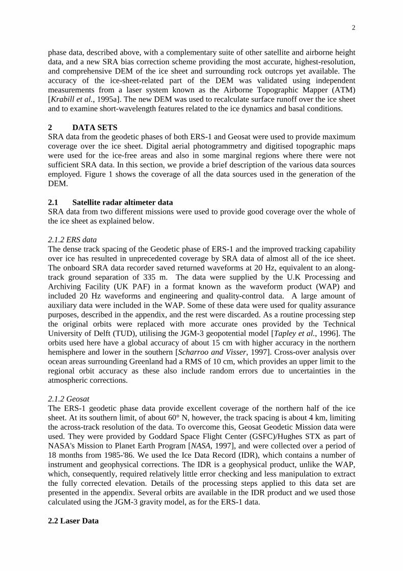
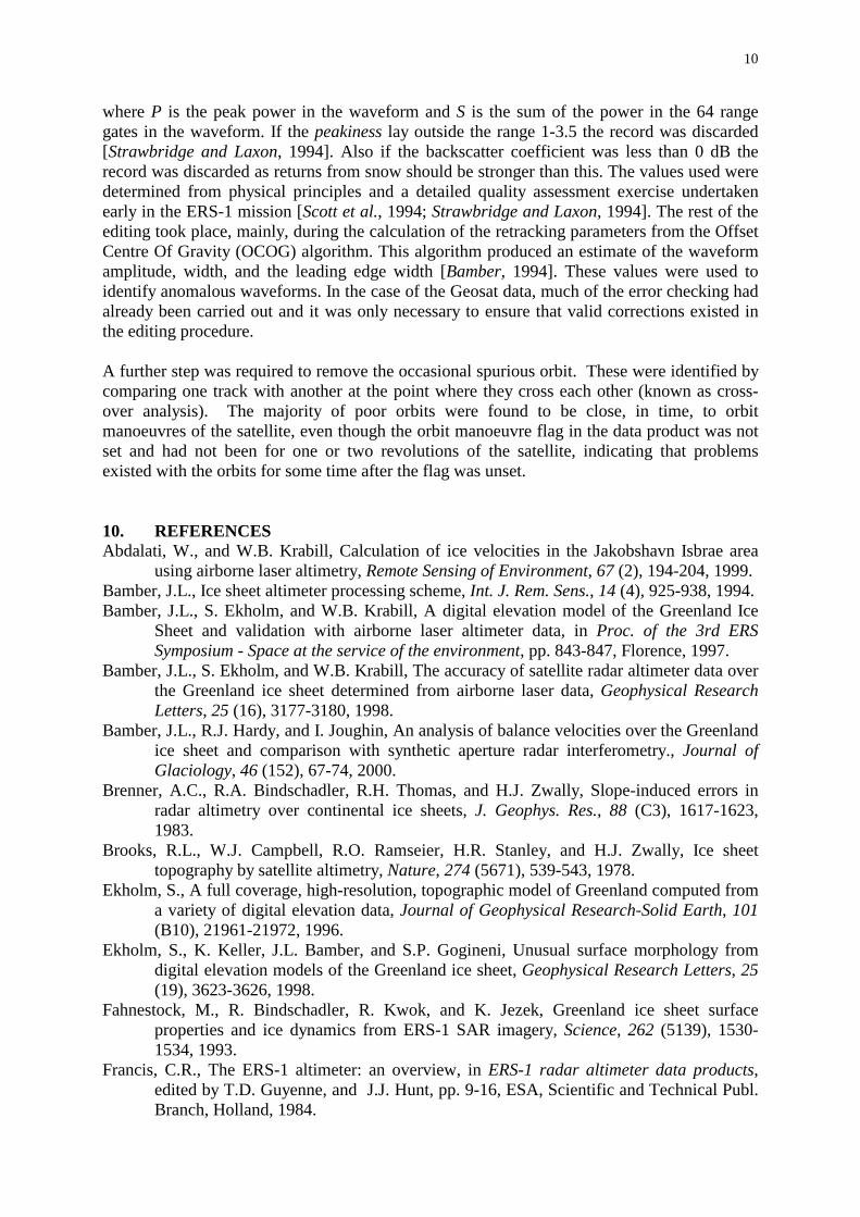
FIGURE CAPTIONS Figure 1. Coverage of different data sources used in the generation of the DEM. The colours used have the following meaning: black is ERS-1data, dark blue Geosat, light blue is KMS-photogrammetry, dark green, light green, and yellow are GEUS photogrammetry. The different colours are for data collected at different times. Scattered red is KMS-map digitisations, dense red and dark orange is unclassified DTED-0 data and light orange is SAR interferometry. Figure 2. Coverage of the airborne laser data used to validate the DEM over the ice sheet. Figure 3. Plot of standard deviations of high-pass filtered airborne laser data as a function of surface slope for 0.02˚ slope intervals. Figure 4a. Plot of standard deviations and biases for the comparison between the airborne laser and satellite radar altimeter data before adjustment (open circles and open squares respectively) and after adjustment (solid squares). The standard deviation after adjustment is not shown as it is almost identical to the values plotted before adjustment. Figure 4b As for figure 4a but here the standard deviations and biases are between the airborne laser data and the DEM. Also plotted, using a logarithmic scale, are the number of airborne laser points at each slope interval used to compute the statistics. Figure 5. Relief-shaded planimetric view of the whole DEM for Greenland in a universal transverse mercator projection. Non ice-covered areas are shown in shades of green and brown. The yellow boxes indicate the approximate location of the subsets plotted in Figure 5. Figure 6 a) Oblique relief-shaded view of the north-west sector of the ice sheet, covering Humboldt, Petermann and Ryder Gletschers. The scale on the axes is in units of grid cells and is equivalent, therefore, to kilometres. b) Oblique relief-shaded view of a sector east of and overlapping a). c) Oblique relief-shaded view of a sector covering the north-east ice stream and its drainage basin. d) Oblique relief-shaded view of the southern tip of Greenland. Figure 7. A plot of height "anomalies" derived by subtracting the DEM from a version smoothed over twenty times the local ice thickness. Figure A1 Structure of the tesseral cells used in the slopes database. Three levels of the tesselation are represented. There are four smallest cells shown by the dotted lines. The dashed lines outline two cells at the next level in the tesselation and the solid line indicates a single cell at the next level again. The longer side of each rectangular cell is √2 times the shorter side. Figure A2 a) Flow diagram showing the main steps in the ERS-1 SRA processing scheme b) Flow diagram showing the main steps in the Geosat SRA processing scheme The following acronyms have been used in the diagram and text: GSFC Goddard Space Flight Center IDR Instrument Data Record JGM Joint Gravity Model OCOG Offset Centre Of Gravity WAP Waveform Product TUD Technical University of Delft

14

Figure 1 Figure 2

15

16

Figure 5.

Figure 6

17

18