________________________________________________________________________ Danielson, Tyler. 2013. Utilizing a High Resolution Digital Elevation Model (DEM) to Apply Stream Power

Index (SPI) to the Gilmore Creek Watershed in Winona County, Minnesota. Volume 15, Papers in Resource

Analysis. 11 pp. Saint Mary’s University of Minnesota University Central Services Press. Winona, MN.

Retrieved (date) http://www.gis.smumn.edu

Utilizing a High Resolution Digital Elevation Model (DEM) to Develop a Stream Power

Index (SPI) for the Gilmore Creek Watershed in Winona County, Minnesota

Tyler Danielson

Department of Resource Analysis, Saint Mary’s University of Minnesota, Winona, MN 55987

Keywords: GIS, Winona County, Agriculture, Erosion, ArcGIS, Slope, Aspect, Flow

Direction, Flow Accumulation, Stream Point Index, SPI, Critical Threshold, Digital

Elevation Model, DEM, LiDAR, Gully Erosion

Abstract

Erosion on the landscape usually happens in small increments and over thousands of years.

With the advent of the agricultural and industrial revolutions many areas within the United

States have witnessed increased top soil erosion. Much of this erosion has originated on

agricultural lands, usually being attributed to the lack of adequate ground cover and not

taking advantage of “best management practices.” These “best management practices”

include: terracing, conservation dams and/or grass flow ways. The objective of this project

was to utilize a high resolution digital elevation model developed using LiDAR (Light

detection and ranging) paired with the SPI model of erosion prediction to test the model’s

applicability to an entire watershed as a way to quickly identify areas at risk of gully erosion.

Introduction

Topography defines the pathways of

surface water movement across a

watershed and is a major factor watershed

hydrologic response to rainfall inputs.

Raster-based digital elevation models

(DEMs) have been widely applied to

efficiently derive topographic attributes

used in hydrologic modeling such as slope

and upslope contributing area (Wu, Li, and

Huang, 2008). Numerous soil erosion

models have been developed during the

last fifty years to estimate rates of soil

erosion under different land use systems

(Wilson and Lorang, 2000).

Erosion analysis models such as

USLE (Universal Soil Loss Equation) and

RUSLE (Revised Universal Soil Loss

Equation) developed and used by the

United States Department of Agriculture

(USDA) can be very cumbersome in

practice.

USLE is a multiplicative model

that was empirically derived from over

10,000 plot years of data (Wischmeier and

Smith, 1965; Wischmeier, 1976). The

equation consists of the following formula:

Where A is the mean soil loss in

tons per hectare over the entire slope

length, R is the rainfall-runoff erosivity

factor, K is the soil erodibility factor, C is

a cover management factor, P is a

supporting practices factor, L is a slope

length factor and S is a slope steepness

factor. R is the product of the storm total

kinetic energy and the maximum 30

minute intensity for qualifying storms

(Meyer, 1984; USDA 2013).

2

The model is used to compare soil

erosion from individual farm fields to that

expected from a ‘standard’ soil-loss plot.

The USLE defines soil loss as the amount

of eroded soil and how far it has moved

down slope (Yoder and Lown, 1995).

RUSLE retains the basic structure of the

original model but incorporated new factor

values that were based on the analysis of

thousands of new erosion measurements

(Renard, Foster, Weesies, and Porter,

1991; Renard, Foster, Weesies, McCool,

and Yoder, 1993; Renard, Foster, Yoder,

and McCool, 1994).

In general, the improvements to the

USLE model included; revising the R

factor values, allowing the ability to adjust

K and C factor values and to improve the

LS factor equations.

These models calculate the mass of

soil eroded by a rain event. This can be

helpful in many instances. However in

other instances, it may not be important to

know exactly how many tons of soil were

moved during an event but rather knowing

the spatial location of where gully erosion

is occurring on the landscape thus

allowing a land manager to more quickly

and effectively mitigate the erosion issue.

In contrast, to the efforts during the

last decades to investigate sheet and rill

soil erosion processes, relatively few

studies have been focused on quantifying

and/or predicting gully erosion. The

expansion of the use of modern spatial

information technologies such as

geographical information systems (GIS),

digital elevation modeling (DEM) and

remote sensing have created new

possibilities for research in this field

(Martinez-Casasnovas, 2003).

Terrain Analysis

LiDAR based DEM data allows the cell

resolution to be as small as 1 meter, this

brings a dataset with 900 times more detail

than a 30 meter resolution DEM (Nelson,

2010).

High resolution data allows

predictions of erosion without the need of

lengthy volume calculations. Digital

Terrain Analysis (DTA or TA) can be used

as a way to interpret LiDAR elevation

data. DTA is a remote sensing

methodology that combines DEM-based

topographic data analysis in GIS with

imagery, field-based observation and the

study of landscape processes. The purpose

of Digital Terrain Analysis is to predict

landscape processes reliably while

minimizing the time and effort invested in

field work and modeling procedures

(Dogwiler, Dockter, and Omoth, 2010).

Primary attributes are calculated

directly from elevation data. These include

aspect, slope, and flow accumulation as

well many others. Stream Power Index

(SPI) is a secondary attribute calculated

from several primary attributes. Secondary

or compound attributes involve the

combinations of primary attributes; these

are indices (Nelson, 2010). Indices

describe the spatial variability of specific

landscape processes, such as the potential

for sheet erosion (Moore, Grayson, and

Ladson, 1991).

According to Wilson and Lorang

(2000) SPI is the measure of erosive

power associated with flowing water based

on the assumption that discharge is

proportional to the specific catchment area

and it predicts net erosion in areas of

profile convexity and tangential concavity

(flow acceleration and convergence zones)

as well as the net deposition in areas of

profile concavity (zones of decreasing

flow velocity).

Study Area

The study area for this project was the

3

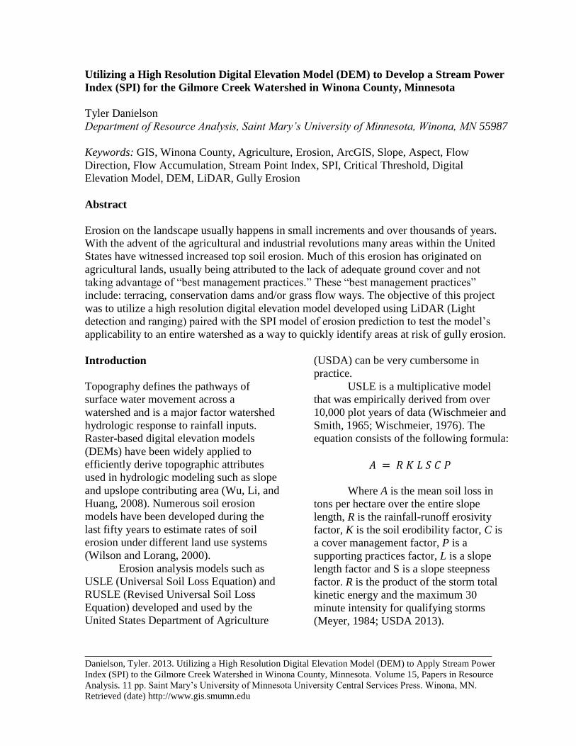
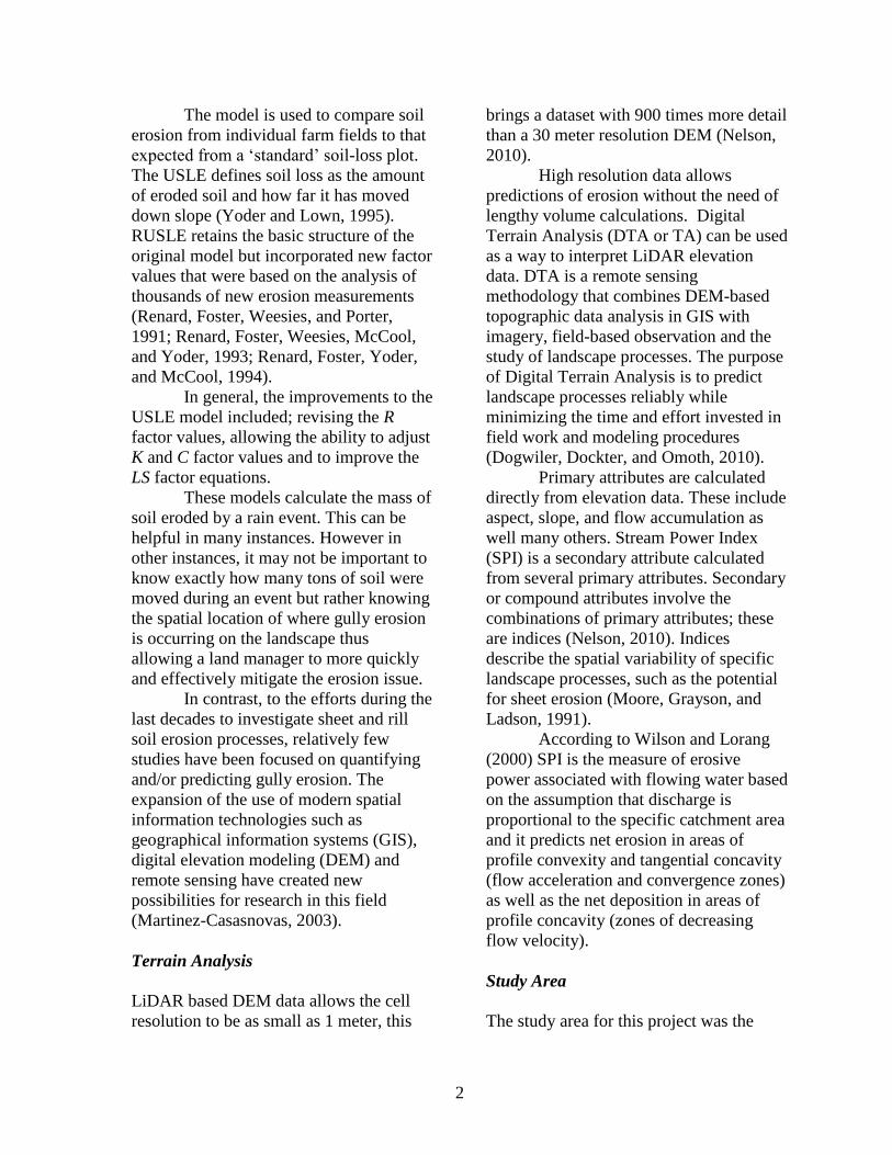
Gilmore Creek, Minnesota, USA

watershed, which is 6216 acres. Gilmore

Creek starts in the hills and bluffs and

flows downstream through the towns of

Goodview and Winona, Minnesota before

draining into the Mississippi River. Large

bluffs dominate the areas between the

farming uplands and the suburban style

subdivision housing developments in the

lower elevations. Nearing the northern

(downstream) portion of the watershed,

Gilmore Creek passes through the Saint

Mary’s University of Minnesota’s Winona

campus (Figures 1 and 2).

Figure 1. General location of the Gilmore Creek

Watershed.

Figure 2. General outline of the Gilmore Creek

Watershed.

Methods/Analysis

Software Used

GIS software used to perform the SPI

analysis were the ESRI ArcGIS v10.1 with

the ESRI Spatial Analyst extension.

GIS Data

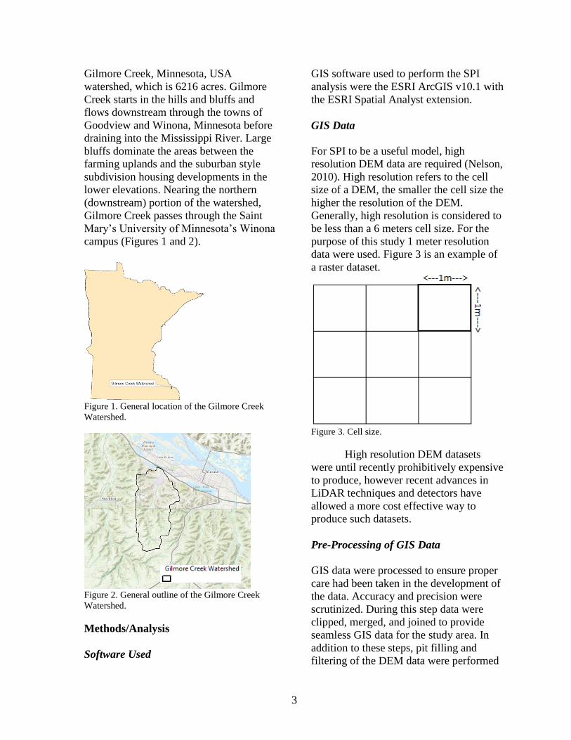
For SPI to be a useful model, high

resolution DEM data are required (Nelson,

2010). High resolution refers to the cell

size of a DEM, the smaller the cell size the

higher the resolution of the DEM.

Generally, high resolution is considered to

be less than a 6 meters cell size. For the

purpose of this study 1 meter resolution

data were used. Figure 3 is an example of

a raster dataset.

Figure 3. Cell size.

High resolution DEM datasets

were until recently prohibitively expensive

to produce, however recent advances in

LiDAR techniques and detectors have

allowed a more cost effective way to

produce such datasets.

Pre-Processing of GIS Data

GIS data were processed to ensure proper

care had been taken in the development of

the data. Accuracy and precision were

scrutinized. During this step data were

clipped, merged, and joined to provide

seamless GIS data for the study area. In

addition to these steps, pit filling and

filtering of the DEM data were performed

4

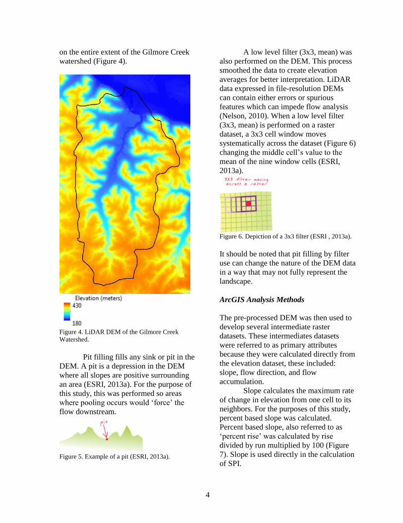
on the entire extent of the Gilmore Creek

watershed (Figure 4).

Figure 4. LiDAR DEM of the Gilmore Creek

Watershed.

Pit filling fills any sink or pit in the

DEM. A pit is a depression in the DEM

where all slopes are positive surrounding

an area (ESRI, 2013a). For the purpose of

this study, this was performed so areas

where pooling occurs would ‘force’ the

flow downstream.

Figure 5. Example of a pit (ESRI, 2013a).

A low level filter (3x3, mean) was

also performed on the DEM. This process

smoothed the data to create elevation

averages for better interpretation. LiDAR

data expressed in file-resolution DEMs

can contain either errors or spurious

features which can impede flow analysis

(Nelson, 2010). When a low level filter

(3x3, mean) is performed on a raster

dataset, a 3x3 cell window moves

systematically across the dataset (Figure 6)

changing the middle cell’s value to the

mean of the nine window cells (ESRI,

2013a).

Figure 6. Depiction of a 3x3 filter (ESRI , 2013a).

It should be noted that pit filling by filter

use can change the nature of the DEM data

in a way that may not fully represent the

landscape.

ArcGIS Analysis Methods

The pre-processed DEM was then used to

develop several intermediate raster

datasets. These intermediates datasets

were referred to as primary attributes

because they were calculated directly from

the elevation dataset, these included:

slope, flow direction, and flow

accumulation.

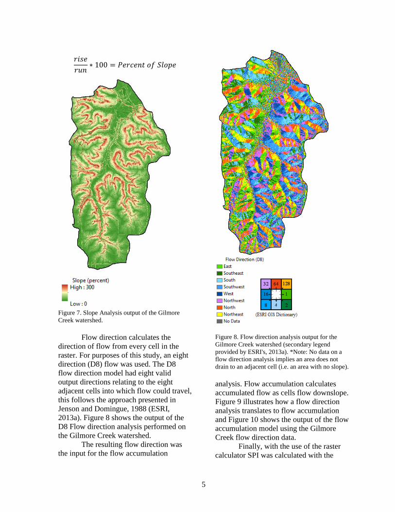
Slope calculates the maximum rate

of change in elevation from one cell to its

neighbors. For the purposes of this study,

percent based slope was calculated.

Percent based slope, also referred to as

‘percent rise’ was calculated by rise

divided by run multiplied by 100 (Figure

7). Slope is used directly in the calculation

of SPI.

5

Figure 7. Slope Analysis output of the Gilmore

Creek watershed.

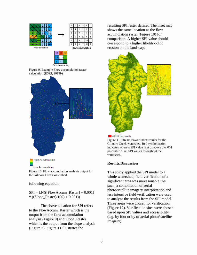
Flow direction calculates the

direction of flow from every cell in the

raster. For purposes of this study, an eight

direction (D8) flow was used. The D8

flow direction model had eight valid

output directions relating to the eight

adjacent cells into which flow could travel,

this follows the approach presented in

Jenson and Domingue, 1988 (ESRI,

2013a). Figure 8 shows the output of the

D8 Flow direction analysis performed on

the Gilmore Creek watershed.

The resulting flow direction was

the input for the flow accumulation

Figure 8. Flow direction analysis output for the

Gilmore Creek watershed (secondary legend

provided by ESRI's, 2013a). *Note: No data on a

flow direction analysis implies an area does not

drain to an adjacent cell (i.e. an area with no slope).

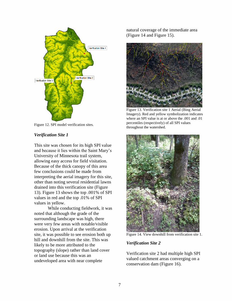
analysis. Flow accumulation calculates

accumulated flow as cells flow downslope.

Figure 9 illustrates how a flow direction

analysis translates to flow accumulation

and Figure 10 shows the output of the flow

accumulation model using the Gilmore

Creek flow direction data.

Finally, with the use of the raster

calculator SPI was calculated with the

6

Figure 9. Example Flow accumulation raster

calculation (ESRI, 2013b).

Figure 10. Flow accumulation analysis output for

the Gilmore Creek watershed.

following equation:

SPI = LN(([FlowAccum_Raster] + 0.001)

* ((Slope_Raster]/100) + 0.001))

The above equation for SPI refers

to the FlowAccum_Raster which is the

output from the flow accumulation

analysis (Figure 9) and Slope_Raster

which is the output from the slope analysis

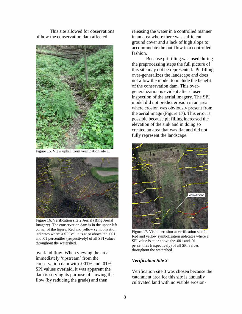
(Figure 7). Figure 11 illustrates the

resulting SPI raster dataset. The inset map

shows the same location as the flow

accumulation raster (Figure 10) for

comparison. A higher SPI value should

correspond to a higher likelihood of

erosion on the landscape.

Figure 11. Stream Power Index results for the

Gilmore Creek watershed. Red symbolization

indicates where a SPI value is at or above the .001

percentile of all SPI values throughout the

watershed.

Results/Discussion

This study applied the SPI model to a

whole watershed; field verification of a

significant area was unreasonable. As

such, a combination of aerial

photo/satellite imagery interpretation and

less intensive field verification were used

to analyze the results from the SPI model.

Three areas were chosen for verification

(Figure 12). Verification sites were chosen

based upon SPI values and accessibility

(e.g. by foot or by of aerial photo/satellite

imagery).

7

Figure 12. SPI model verification sites.

Verification Site 1

This site was chosen for its high SPI value

and because it lies within the Saint Mary’s

University of Minnesota trail system,

allowing easy access for field visitation.

Because of the thick canopy of this area

few conclusions could be made from

interpreting the aerial imagery for this site,

other than noting several residential lawns

drained into this verification site (Figure

13). Figure 13 shows the top .001% of SPI

values in red and the top .01% of SPI

values in yellow.

While conducting fieldwork, it was

noted that although the grade of the

surrounding landscape was high, there

were very few areas with notable/visible

erosion. Upon arrival at the verification

site, it was possible to see erosion both up

hill and downhill from the site. This was

likely to be more attributed to the

topography (slope) rather than land cover

or land use because this was an

undeveloped area with near complete

natural coverage of the immediate area

(Figure 14 and Figure 15).

Figure 13. Verification site 1 Aerial (Bing Aerial

Imagery). Red and yellow symbolization indicates

where an SPI value is at or above the .001 and .01

percentiles (respectively) of all SPI values

throughout the watershed.

Figure 14. View downhill from verification site 1.

Verification Site 2

Verification site 2 had multiple high SPI

valued catchment areas converging on a

conservation dam (Figure 16).

8

This site allowed for observations

of how the conservation dam affected

Figure 15. View uphill from verification site 1.

Figure 16. Verification site 2 Aerial (Bing Aerial

Imagery). The conservation dam is in the upper left

corner of the figure. Red and yellow symbolization

indicates where a SPI value is at or above the .001

and .01 percentiles (respectively) of all SPI values

throughout the watershed.

overland flow. When viewing the area

immediately ‘upstream’ from the

conservation dam with .001% and .01%

SPI values overlaid, it was apparent the

dam is serving its purpose of slowing the

flow (by reducing the grade) and then

releasing the water in a controlled manner

in an area where there was sufficient

ground cover and a lack of high slope to

accommodate the out-flow in a controlled

fashion.

Because pit filling was used during

the preprocessing steps the full picture of

this site may not be represented. Pit filling

over-generalizes the landscape and does

not allow the model to include the benefit

of the conservation dam. This over-

generalization is evident after closer

inspection of the aerial imagery. The SPI

model did not predict erosion in an area

where erosion was obviously present from

the aerial image (Figure 17). This error is

possible because pit filling increased the

elevation of the sink and in doing so

created an area that was flat and did not

fully represent the landscape.

Figure 17. Visible erosion at verification site 2.

Red and yellow symbolization indicates where a

SPI value is at or above the .001 and .01

percentiles (respectively) of all SPI values

throughout the watershed.

Verification Site 3

Verification site 3 was chosen because the

catchment area for this site is annually

cultivated land with no visible erosion-

9

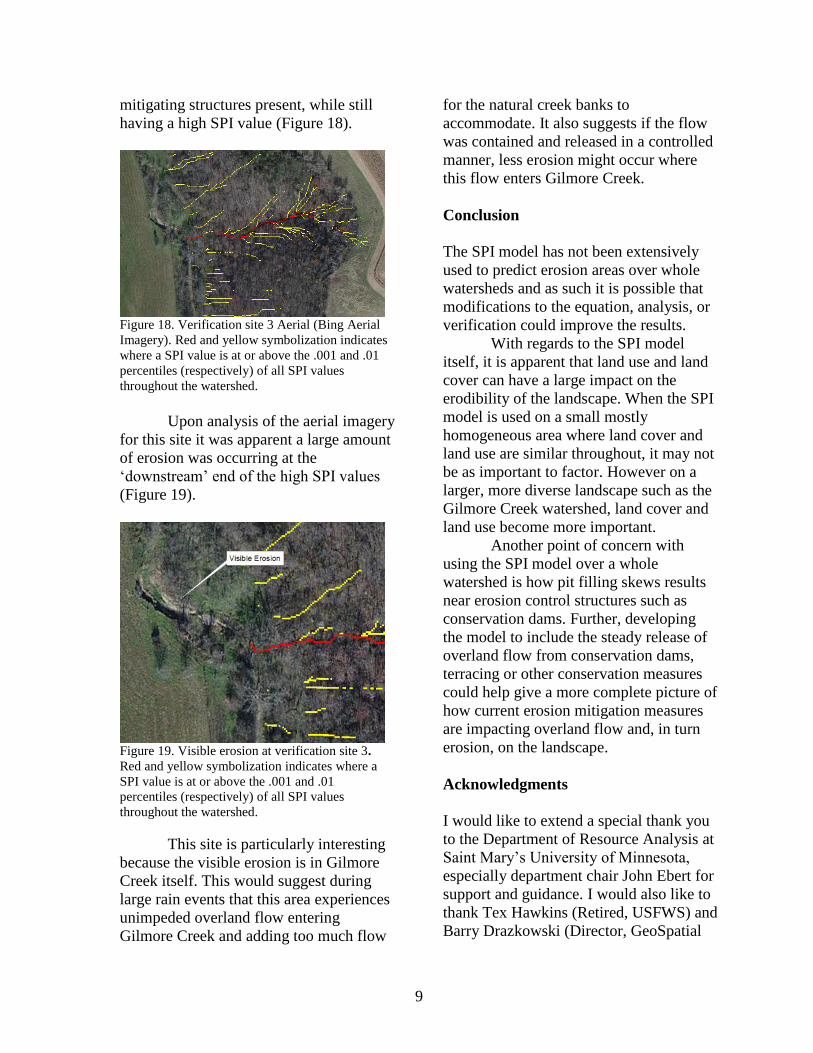
mitigating structures present, while still

having a high SPI value (Figure 18).

Figure 18. Verification site 3 Aerial (Bing Aerial

Imagery). Red and yellow symbolization indicates

where a SPI value is at or above the .001 and .01

percentiles (respectively) of all SPI values

throughout the watershed.

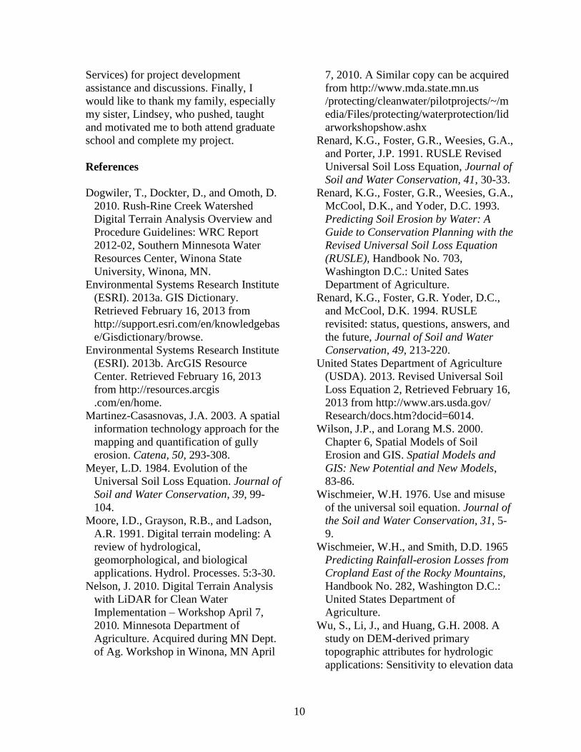
Upon analysis of the aerial imagery

for this site it was apparent a large amount

of erosion was occurring at the

‘downstream’ end of the high SPI values

(Figure 19).

Figure 19. Visible erosion at verification site 3.

Red and yellow symbolization indicates where a

SPI value is at or above the .001 and .01

percentiles (respectively) of all SPI values

throughout the watershed.

This site is particularly interesting

because the visible erosion is in Gilmore

Creek itself. This would suggest during

large rain events that this area experiences

unimpeded overland flow entering

Gilmore Creek and adding too much flow

for the natural creek banks to

accommodate. It also suggests if the flow

was contained and released in a controlled

manner, less erosion might occur where

this flow enters Gilmore Creek.

Conclusion

The SPI model has not been extensively

used to predict erosion areas over whole

watersheds and as such it is possible that

modifications to the equation, analysis, or

verification could improve the results.

With regards to the SPI model

itself, it is apparent that land use and land

cover can have a large impact on the

erodibility of the landscape. When the SPI

model is used on a small mostly

homogeneous area where land cover and

land use are similar throughout, it may not

be as important to factor. However on a

larger, more diverse landscape such as the

Gilmore Creek watershed, land cover and

land use become more important.

Another point of concern with

using the SPI model over a whole

watershed is how pit filling skews results

near erosion control structures such as

conservation dams. Further, developing

the model to include the steady release of

overland flow from conservation dams,

terracing or other conservation measures

could help give a more complete picture of

how current erosion mitigation measures

are impacting overland flow and, in turn

erosion, on the landscape.

Acknowledgments

I would like to extend a special thank you

to the Department of Resource Analysis at

Saint Mary’s University of Minnesota,

especially department chair John Ebert for

support and guidance. I would also like to

thank Tex Hawkins (Retired, USFWS) and

Barry Drazkowski (Director, GeoSpatial

10

Services) for project development

assistance and discussions. Finally, I

would like to thank my family, especially

my sister, Lindsey, who pushed, taught

and motivated me to both attend graduate

school and complete my project.

References

Dogwiler, T., Dockter, D., and Omoth, D.

2010. Rush-Rine Creek Watershed

Digital Terrain Analysis Overview and

Procedure Guidelines: WRC Report

2012-02, Southern Minnesota Water

Resources Center, Winona State

University, Winona, MN.

Environmental Systems Research Institute

(ESRI). 2013a. GIS Dictionary.

Retrieved February 16, 2013 from

http://support.esri.com/en/knowledgebas

e/Gisdictionary/browse.

Environmental Systems Research Institute

(ESRI). 2013b. ArcGIS Resource

Center. Retrieved February 16, 2013

from http://resources.arcgis

.com/en/home.

Martinez-Casasnovas, J.A. 2003. A spatial

information technology approach for the

mapping and quantification of gully

erosion. Catena, 50, 293-308.

Meyer, L.D. 1984. Evolution of the

Universal Soil Loss Equation. Journal of

Soil and Water Conservation, 39, 99-

104.

Moore, I.D., Grayson, R.B., and Ladson,

A.R. 1991. Digital terrain modeling: A

review of hydrological,

geomorphological, and biological

applications. Hydrol. Processes. 5:3-30.

Nelson, J. 2010. Digital Terrain Analysis

with LiDAR for Clean Water

Implementation – Workshop April 7,

2010. Minnesota Department of

Agriculture. Acquired during MN Dept.

of Ag. Workshop in Winona, MN April

7, 2010. A Similar copy can be acquired

from http://www.mda.state.mn.us

/protecting/cleanwater/pilotprojects/~/m

edia/Files/protecting/waterprotection/lid

arworkshopshow.ashx

Renard, K.G., Foster, G.R., Weesies, G.A.,

and Porter, J.P. 1991. RUSLE Revised

Universal Soil Loss Equation, Journal of

Soil and Water Conservation, 41, 30-33.

Renard, K.G., Foster, G.R., Weesies, G.A.,

McCool, D.K., and Yoder, D.C. 1993.

Predicting Soil Erosion by Water: A

Guide to Conservation Planning with the

Revised Universal Soil Loss Equation

(RUSLE), Handbook No. 703,

Washington D.C.: United Sates

Department of Agriculture.

Renard, K.G., Foster, G.R. Yoder, D.C.,

and McCool, D.K. 1994. RUSLE

revisited: status, questions, answers, and

the future, Journal of Soil and Water

Conservation, 49, 213-220.

United States Department of Agriculture

(USDA). 2013. Revised Universal Soil

Loss Equation 2, Retrieved February 16,

2013 from http://www.ars.usda.gov/

Research/docs.htm?docid=6014.

Wilson, J.P., and Lorang M.S. 2000.

Chapter 6, Spatial Models of Soil

Erosion and GIS. Spatial Models and

GIS: New Potential and New Models,

83-86.

Wischmeier, W.H. 1976. Use and misuse

of the universal soil equation. Journal of

the Soil and Water Conservation, 31, 5-

9.

Wischmeier, W.H., and Smith, D.D. 1965

Predicting Rainfall-erosion Losses from

Cropland East of the Rocky Mountains,

Handbook No. 282, Washington D.C.:

United States Department of

Agriculture.

Wu, S., Li, J., and Huang, G.H. 2008. A

study on DEM-derived primary

topographic attributes for hydrologic

applications: Sensitivity to elevation data

11

resolution, Applied Geography, 28, 210-

223.

Yoder, D., and Lown, J. 1995. The future

of RUSLE: inside the new Revised

Universal Soil Loss Equation, Journal of

Soil and Water Conservation, 50, 484-

489.