2007 annual energy outlook
TRANSCRIPT

7/28/2019 2007 Annual Energy Outlook
http://slidepdf.com/reader/full/2007-annual-energy-outlook 1/243

7/28/2019 2007 Annual Energy Outlook
http://slidepdf.com/reader/full/2007-annual-energy-outlook 2/243
DOE/EIA-0383(2007)
February 2007
Annual Energy Outlook 2007 With Projections to 2030
Energy Information Administration
Office of Integrated Analysis and Forecasting
U.S. Department of Energy
Washington, DC 20585

7/28/2019 2007 Annual Energy Outlook
http://slidepdf.com/reader/full/2007-annual-energy-outlook 3/243
For Further Information . . .
The Annual Energy Outlook 2007 was prepared by the Energy Information Administration, under the direc-tion of John J. Conti ([email protected], 202-586-2222), Director, Integrated Analysis and Forecasting;
Paul D. Holtberg ([email protected], 202/586-1284), Director, Demand and Integration Division; Joseph A. Beamon ([email protected], 202/586-2025), Director, Coal and Electric Power Division; A. Michael Schaal ([email protected], 202/586-5590), Director, Oil and Gas Division; Glen E.Sweetnam ([email protected], 202/586-2188), Director, International, Economic, and GreenhouseGases Division; and Andy S. Kydes ([email protected], 202/586-2222), Senior Technical Advisor.
For ordering information and questions on other energy statistics available from the Energy Information
Administration, please contact the National Energy Information Center. Addresses, telephone numbers, andhours are as follows:
National Energy Information Center, EI-30Energy Information AdministrationForrestal Building
Washington, DC 20585Telephone: 202/586-8800 E-mail: [email protected]: 202/586-0727 Web Site: http://www.eia.doe.gov/ TTY: 202/586-1181 FTP Site: ftp://ftp.eia.doe.gov/ 9 a.m. to 5 p.m., eastern time, M-F
Specific questions about the information in this report may be directed to:
Overview . . . . . . . . . . . . . . . Paul D. Holtberg ([email protected], 202/586-1284)
Economic Activity . . . . . . . . . . Ronald F. Earley ([email protected], 202/586-1398)International Oil Markets . . . . . . John L. Staub ([email protected], 202/586-6344)Residential Demand . . . . . . . . . John H. Cymbalsky ([email protected], 202/586-4815)Commercial Demand . . . . . . . . . Erin E. Boedecker ([email protected], 202/586-4791)
Industrial Demand . . . . . . . . . . T. Crawford Honeycutt ([email protected], 202/586-1420)Transportation Demand . . . . . . . John D. Maples ([email protected], 202/586-1757)Electricity Generation, Capacity. . . Jeff S. Jones ([email protected], 202/586-2038)Electricity Generation, Emissions . . Robert K. Smith ([email protected], 202/586-9413)Electricity Prices . . . . . . . . . . . Lori B. Aniti ([email protected], 202/586-2867)
Nuclear Energy . . . . . . . . . . . . Laura K. Martin ([email protected], 202/586-1494)Renewable Energy . . . . . . . . . . Chris R. Namovicz ([email protected], 202/586-7120)Oil and Natural Gas Production . . . Eddie L. Thomas, Jr. ([email protected], 202/586-5877)Natural Gas Markets . . . . . . . . . Philip M. Budzik ([email protected], 202/586-2847)Oil Refining and Markets . . . . . . Albert J. Walgreen ([email protected], 202/586-5748)Coal Supply and Prices. . . . . . . . Michael L. Mellish ([email protected], 202/586-2136)Greenhouse Gas Emissions . . . . . Daniel H. Skelly ([email protected], 202/586-1722)
The Annual Energy Outlook 2007 will be available on the EIA web site at www.eia.doe.gov/oiaf/aeo/ in early2007. Assumptions underlying the projections, tables of regional results, and other detailed results will also beavailable in early 2007, at web sites www.eia.doe.gov/oiaf/assumption/ and /supplement/. Model documenta-tion reports for the National Energy Modeling System are available at web site www.eia.doe.gov/bookshelf/ docs.html and will be updated for the Annual Energy Outlook 2007 during the first few months of 2007.
Other contributors to the report include Joseph Benneche, Bill Brown, John Cochener, Margie Daymude,
Linda Doman, Robert Eynon, Bryan Haney, James Hewlett, Elizabeth Hossner, Diane Kearney, Nasir Khilji,Paul Kondis, Thomas Lee, Phyllis Martin, Ted McCallister, Chetha Phang, Anthony Radich, Eugene Reiser,Laurence Sanders, Bhima Sastri, Sharon Shears, Yvonne Taylor, Brian Unruh, Dana Van Wagener, Steven
Wade, Peggy Wells, and Peter Whitman.

7/28/2019 2007 Annual Energy Outlook
http://slidepdf.com/reader/full/2007-annual-energy-outlook 4/243
DOE/EIA-0383(2007)
Annual Energy Outlook 2007
With Projections to 2030
February 2007
Energy Information Administration
Office of Integrated Analysis and Forecasting
U.S. Department of Energy
Washington, DC 20585
This report was prepared by the Energy Information Administration, the independent statistical and
analytical agency within the U.S. Department of Energy. The information contained herein should be
attributed to the Energy Information Administration and should not be construed as advocating or
reflecting any policy position of the Department of Energy or any other organization.
This publication is on the WEB at:www.eia.doe.gov/oiaf/aeo/

7/28/2019 2007 Annual Energy Outlook
http://slidepdf.com/reader/full/2007-annual-energy-outlook 5/243
The Annual Energy Outlook 2007 ( AEO2007 ), pre-pared by the Energy Information Administration(EIA), presents long-term projections of energy sup-
ply, demand, and prices through 2030. The projec-tions are based on results from EIA’s National
Energy Modeling System (NEMS).
The report begins with an “Overview” summarizing the AEO2007 reference case. The next section, “Leg-islation and Regulations,” discusses evolving legisla-tion and regulatory issues, including recently enactedlegislation and regulation, such as the new Corporate
Average Fuel Economy (CAFE) standards for light-
duty trucks finalized by the National Highway TrafficSafety Administration (NHTSA) in March 2006. Italso provides an update on the handling of key provi-sions in the Energy Policy Act of 2005 (EPACT2005)
that could not be incorporated in the Annual EnergyOutlook 2006 ( AEO2006) because of the absence of implementing regulations or funding appropriations.Finally, it provides a summary of how sunset provi-sions in selected Federal fuel taxes and tax credits are
handled in AEO2007 .
The “Issues in Focus” section includes discussions of the potential for biofuels in U.S. transportation mar-kets, the relationship between oil and natural gasprices, and the impact of rising construction costs onenergy markets. It also discusses possible construc-tion of an Alaska natural gas pipeline; renewed inter-
est in nuclear generating capacity; and the demandresponse to higher energy prices in end-use sectors.
The “Market Trends” section summarizes the AEO-
2007 projections for energy markets. The projectionsfor 2006 and 2007 incorporate the short-term projec-tions from EIA’s September 2006 Short-Term Energy
Outlook, where the data are comparable. The analysisin AEO2007 focuses primarily on a reference case,lower and higher economic growth cases, and lower
and higher energy price cases. Results from a numberof other alternative cases are also presented, illustrat-
ing uncertainties associated with the reference caseprojections for energy demand, supply, and prices.Readers are encouraged to review the full range of cases, which address many of the uncertainties inher-ent in long-term projections. Complete tables for thefive primary cases are provided in Appendixes A through C. Major results from many of the alterna-
tive cases are provided in Appendix D. Appendix Ebriefly describes NEMS and the alternative cases.
AEO2007 projections generally are based on Federal,State, and local laws and regulations in effect on or
before October 31, 2006. The potential impacts of
pending or proposed legislation, regulations, andstandards (and sections of existing legislation that re-quire implementing regulations or funds that havenot been appropriated) are not reflected in theprojections.
In general, historical data used in the AEO2006 pro- jections are based on EIA’s Annual Energy Review
2005 , published in August 2006; however, only partialor preliminary 2005 data were available in somecases. Other historical data, taken from multiplesources, are presented in this report for comparativepurposes; documents referenced in the source notesshould be consulted for official data values.
AEO2007 is published in accordance with Section205c of the Department of Energy Organization Actof 1977 (Public Law 95-91), which requires the EIA
Administrator to prepare annual reports on trends
and projections for energy use and supply.
ii Energy Information Administration / Annual Energy Outlook 2007
Preface
The projections in the Annual Energy Outlook 2007 arenot statements of what will happen but of what mighthappen, given the assumptions and methodologies used.The projections are business-as-usual trend estimates,given known technology and technological and demo-graphic trends. AEO2007 generally assumes that current
laws and regulations are maintained throughout the pro- jections. Thus, the projections provide a policy-neutralreference case that can be used to analyze policy initia-tives. EIA does not propose, advocate, or speculate onfuture legislative and regulatory changes. Most laws areassumed to remain as currently enacted; however, theimpacts of emerging regulatory changes, when defined,are reflected.
Because energy markets are complex, models are simpli-fied representations of energy production and con-sumption, regulations, and producer and consumerbehavior. Projections are highly dependent on the data,
methodologies, model structures, and assumptions used intheir development. Behavioral characteristics are indica-tive of real-world tendencies rather than representationsof specific outcomes.
Energy market projections are subject to much uncer-
tainty. Many of the events that shape energy markets arerandom and cannot be anticipated, including severeweather, political disruptions, strikes, and technologicalbreakthroughs. In addition, future developments in tech-nologies, demographics, and resources cannot be foreseenwith certainty. Many key uncertainties in the AEO2007 projections are addressed through alternative cases.
EIA has endeavored to make these projections as objective,reliable, and useful as possible; however, they should serveas an adjunct to, not a substitute for, a complete andfocused analysis of public policy initiatives.

7/28/2019 2007 Annual Energy Outlook
http://slidepdf.com/reader/full/2007-annual-energy-outlook 6/243
Page
Overview . . . . . . . . . . . . . . . . . . . . . . . . . . . . . . . . . . . . . . . . . . . . . . . . . . . . . . . . . . . . . . . . . . . . . . . . . . 1
Legislation and Regulations . . . . . . . . . . . . . . . . . . . . . . . . . . . . . . . . . . . . . . . . . . . . . . . . . . . . . . . . . . 15
Issues in Focus . . . . . . . . . . . . . . . . . . . . . . . . . . . . . . . . . . . . . . . . . . . . . . . . . . . . . . . . . . . . . . . . . . . . . 33
Market Trends. . . . . . . . . . . . . . . . . . . . . . . . . . . . . . . . . . . . . . . . . . . . . . . . . . . . . . . . . . . . . . . . . . . . . . 67
Energy Information Administration / Annual Energy Outlook 2007 iii
Contents
Energy Trends to 2030 . . . . . . . . . . . . . . . . . . . . . . . . . . . . . . . . . . . . . . . . . . . . . . . . . . . . . . . . . . . . . . . . . . 2Economic Growth. . . . . . . . . . . . . . . . . . . . . . . . . . . . . . . . . . . . . . . . . . . . . . . . . . . . . . . . . . . . . . . . . . . . . . . 4Energy Prices . . . . . . . . . . . . . . . . . . . . . . . . . . . . . . . . . . . . . . . . . . . . . . . . . . . . . . . . . . . . . . . . . . . . . . . . . . 4Energy Consumption . . . . . . . . . . . . . . . . . . . . . . . . . . . . . . . . . . . . . . . . . . . . . . . . . . . . . . . . . . . . . . . . . . . . 6Energy Intensity . . . . . . . . . . . . . . . . . . . . . . . . . . . . . . . . . . . . . . . . . . . . . . . . . . . . . . . . . . . . . . . . . . . . . . . 8Electricity Generation . . . . . . . . . . . . . . . . . . . . . . . . . . . . . . . . . . . . . . . . . . . . . . . . . . . . . . . . . . . . . . . . . . . 9Energy Production and Imports . . . . . . . . . . . . . . . . . . . . . . . . . . . . . . . . . . . . . . . . . . . . . . . . . . . . . . . . . . . 10Energy-Related Carbon Dioxide Emissions . . . . . . . . . . . . . . . . . . . . . . . . . . . . . . . . . . . . . . . . . . . . . . . . . . 12
Trends in Economic Activity. . . . . . . . . . . . . . . . . . . . . . . . . . . . . . . . . . . . . . . . . . . . . . . . . . . . . . . . . . . . . . 68International Oil Markets . . . . . . . . . . . . . . . . . . . . . . . . . . . . . . . . . . . . . . . . . . . . . . . . . . . . . . . . . . . . . . . . 70Energy Demand . . . . . . . . . . . . . . . . . . . . . . . . . . . . . . . . . . . . . . . . . . . . . . . . . . . . . . . . . . . . . . . . . . . . . . . . 72Residential Sector Energy Demand . . . . . . . . . . . . . . . . . . . . . . . . . . . . . . . . . . . . . . . . . . . . . . . . . . . . . . . . 74Commercial Sector Energy Demand. . . . . . . . . . . . . . . . . . . . . . . . . . . . . . . . . . . . . . . . . . . . . . . . . . . . . . . . 75Industrial Sector Energy Demand . . . . . . . . . . . . . . . . . . . . . . . . . . . . . . . . . . . . . . . . . . . . . . . . . . . . . . . . . 77Transportation Sector Energy Demand . . . . . . . . . . . . . . . . . . . . . . . . . . . . . . . . . . . . . . . . . . . . . . . . . . . . . 80Electricity Demand and Supply. . . . . . . . . . . . . . . . . . . . . . . . . . . . . . . . . . . . . . . . . . . . . . . . . . . . . . . . . . . . 82
Electricity Supply. . . . . . . . . . . . . . . . . . . . . . . . . . . . . . . . . . . . . . . . . . . . . . . . . . . . . . . . . . . . . . . . . . . . . . . 83Electricity Prices . . . . . . . . . . . . . . . . . . . . . . . . . . . . . . . . . . . . . . . . . . . . . . . . . . . . . . . . . . . . . . . . . . . . . . . 88Natural Gas Demand. . . . . . . . . . . . . . . . . . . . . . . . . . . . . . . . . . . . . . . . . . . . . . . . . . . . . . . . . . . . . . . . . . . . 89Natural Gas Prices. . . . . . . . . . . . . . . . . . . . . . . . . . . . . . . . . . . . . . . . . . . . . . . . . . . . . . . . . . . . . . . . . . . . . . 91Natural Gas Supply . . . . . . . . . . . . . . . . . . . . . . . . . . . . . . . . . . . . . . . . . . . . . . . . . . . . . . . . . . . . . . . . . . . . . 93Oil Production . . . . . . . . . . . . . . . . . . . . . . . . . . . . . . . . . . . . . . . . . . . . . . . . . . . . . . . . . . . . . . . . . . . . . . . . . 95Liquid Fuels Production and Demand . . . . . . . . . . . . . . . . . . . . . . . . . . . . . . . . . . . . . . . . . . . . . . . . . . . . . . 97Coal Production . . . . . . . . . . . . . . . . . . . . . . . . . . . . . . . . . . . . . . . . . . . . . . . . . . . . . . . . . . . . . . . . . . . . . . . . 98Coal Demand and Supply . . . . . . . . . . . . . . . . . . . . . . . . . . . . . . . . . . . . . . . . . . . . . . . . . . . . . . . . . . . . . . . . 99Coal Prices . . . . . . . . . . . . . . . . . . . . . . . . . . . . . . . . . . . . . . . . . . . . . . . . . . . . . . . . . . . . . . . . . . . . . . . . . . . . 100Emissions From Energy Use . . . . . . . . . . . . . . . . . . . . . . . . . . . . . . . . . . . . . . . . . . . . . . . . . . . . . . . . . . . . . . 101
Introduction . . . . . . . . . . . . . . . . . . . . . . . . . . . . . . . . . . . . . . . . . . . . . . . . . . . . . . . . . . . . . . . . . . . . . . . . . . . 16EPACT2005: Status of Provisions . . . . . . . . . . . . . . . . . . . . . . . . . . . . . . . . . . . . . . . . . . . . . . . . . . . . . . . . . 17Fuel Economy Standards for New Light Trucks . . . . . . . . . . . . . . . . . . . . . . . . . . . . . . . . . . . . . . . . . . . . . . 21Regulation of Emissions from Stationary Diesel Engines. . . . . . . . . . . . . . . . . . . . . . . . . . . . . . . . . . . . . . . 23Federal and State Ethanol and Biodiesel Requirements. . . . . . . . . . . . . . . . . . . . . . . . . . . . . . . . . . . . . . . . 23Federal Fuels Taxes and Tax Credits . . . . . . . . . . . . . . . . . . . . . . . . . . . . . . . . . . . . . . . . . . . . . . . . . . . . . . . 24
Electricity Prices in Transition . . . . . . . . . . . . . . . . . . . . . . . . . . . . . . . . . . . . . . . . . . . . . . . . . . . . . . . . . . . . 25State Renewable Energy Requirements and Goals: Update Through 2006. . . . . . . . . . . . . . . . . . . . . . . . . 28State Regulations on Airborne Emissions: Update Through 2006 . . . . . . . . . . . . . . . . . . . . . . . . . . . . . . . . 30
Introduction . . . . . . . . . . . . . . . . . . . . . . . . . . . . . . . . . . . . . . . . . . . . . . . . . . . . . . . . . . . . . . . . . . . . . . . . . . . 34 World Oil Prices in AEO2007 . . . . . . . . . . . . . . . . . . . . . . . . . . . . . . . . . . . . . . . . . . . . . . . . . . . . . . . . . . . . . 34Impacts of Rising Construction and Equipment Costs on Energy Industries . . . . . . . . . . . . . . . . . . . . . . . 36Energy Demand: Limits on the Response to Higher Energy Prices in the End-Use Sectors . . . . . . . . . . . 41Miscellaneous Electricity Services in the Buildings Sector. . . . . . . . . . . . . . . . . . . . . . . . . . . . . . . . . . . . . . 45Industrial Sector Energy Demand: Revisions for Non-Energy-Intensive Manufacturing . . . . . . . . . . . . . 47Loan Guarantees and the Economics of Electricity Generating Technologies . . . . . . . . . . . . . . . . . . . . . . 48Impacts of Increased Access to Oil and Natural Gas Resources in the Lower 48 Federal
Outer Continental Shelf . . . . . . . . . . . . . . . . . . . . . . . . . . . . . . . . . . . . . . . . . . . . . . . . . . . . . . . . . . . . . . . 50 Alaska Natural Gas Pipeline Developments. . . . . . . . . . . . . . . . . . . . . . . . . . . . . . . . . . . . . . . . . . . . . . . . . . 52Coal Transportation Issues . . . . . . . . . . . . . . . . . . . . . . . . . . . . . . . . . . . . . . . . . . . . . . . . . . . . . . . . . . . . . . . 54Biofuels in the U.S. Transportation Sector . . . . . . . . . . . . . . . . . . . . . . . . . . . . . . . . . . . . . . . . . . . . . . . . . . 57

7/28/2019 2007 Annual Energy Outlook
http://slidepdf.com/reader/full/2007-annual-energy-outlook 7/243
Page
Comparison with Other Projections . . . . . . . . . . . . . . . . . . . . . . . . . . . . . . . . . . . . . . . . . . . . . . . . . . . 105
List of Acronyms . . . . . . . . . . . . . . . . . . . . . . . . . . . . . . . . . . . . . . . . . . . . . . . . . . . . . . . . . . . . . . . . . . . . 118
Notes and Sources . . . . . . . . . . . . . . . . . . . . . . . . . . . . . . . . . . . . . . . . . . . . . . . . . . . . . . . . . . . . . . . . . . 119
Appendixes A. Reference Case . . . . . . . . . . . . . . . . . . . . . . . . . . . . . . . . . . . . . . . . . . . . . . . . . . . . . . . . . . . . . . . . . . . . . . 135B. Economic Growth Case Comparisons . . . . . . . . . . . . . . . . . . . . . . . . . . . . . . . . . . . . . . . . . . . . . . . . . . . . 169C. Price Case Comparisons. . . . . . . . . . . . . . . . . . . . . . . . . . . . . . . . . . . . . . . . . . . . . . . . . . . . . . . . . . . . . . . 177D. Results from Side Cases . . . . . . . . . . . . . . . . . . . . . . . . . . . . . . . . . . . . . . . . . . . . . . . . . . . . . . . . . . . . . . . 190E. NEMS Overview and Brief Description of Cases . . . . . . . . . . . . . . . . . . . . . . . . . . . . . . . . . . . . . . . . . . . 207F. Regional Maps. . . . . . . . . . . . . . . . . . . . . . . . . . . . . . . . . . . . . . . . . . . . . . . . . . . . . . . . . . . . . . . . . . . . . . . 221G. Conversion Factors. . . . . . . . . . . . . . . . . . . . . . . . . . . . . . . . . . . . . . . . . . . . . . . . . . . . . . . . . . . . . . . . . . . 229
Tables
Figures
iv Energy Information Administration / Annual Energy Outlook 2007
Contents
1. Total energy supply and disposition in the AEO2007 and AEO2006 reference cases, 2005-2030. . . . . 14
2. Changes in Standard Offer Supply price determinations by supply region and State . . . . . . . . . . . . . . 273. OPEC and non-OPEC oil production in three AEO2007 world oil price cases, 2005-2030 . . . . . . . . . . 364. Changes in surface coal mining equipment costs, 2002-2005 . . . . . . . . . . . . . . . . . . . . . . . . . . . . . . . . . 395. Miscellaneous electricity uses in the residential sector, 2005, 2015, and 2030. . . . . . . . . . . . . . . . . . . . 456. Electricity use and market share for televisions by type, 2005 and 2015 . . . . . . . . . . . . . . . . . . . . . . . . 467. Miscellaneous electricity uses in the commercial sector, 2005, 2015, and 2030 . . . . . . . . . . . . . . . . . . . 468. Revised subgroups for the non-energy-intensive manufacturing industries in AEO2007 :
energy demand and value of shipments, 2002 . . . . . . . . . . . . . . . . . . . . . . . . . . . . . . . . . . . . . . . . . . . . . 479. Effects of DOE’s loan guarantee program on the economics of electric power plant
generating technologies, 2015 . . . . . . . . . . . . . . . . . . . . . . . . . . . . . . . . . . . . . . . . . . . . . . . . . . . . . . . . . . 5010. Technically recoverable undiscovered oil and natural gas resources in the lower 48
Outer Continental Shelf as of January 1, 2003. . . . . . . . . . . . . . . . . . . . . . . . . . . . . . . . . . . . . . . . . . . . . 5111. U.S. motor fuels consumption, 2000-2005. . . . . . . . . . . . . . . . . . . . . . . . . . . . . . . . . . . . . . . . . . . . . . . . . 5712. Energy content of biofuels . . . . . . . . . . . . . . . . . . . . . . . . . . . . . . . . . . . . . . . . . . . . . . . . . . . . . . . . . . . . . 5913. U.S. production and values of biofuel co-products . . . . . . . . . . . . . . . . . . . . . . . . . . . . . . . . . . . . . . . . . . 6214. Vehicle fueling stations in the United States as of July 2006 . . . . . . . . . . . . . . . . . . . . . . . . . . . . . . . . . 6315. Potential U.S. market for biofuel blends, 2005. . . . . . . . . . . . . . . . . . . . . . . . . . . . . . . . . . . . . . . . . . . . . 6416. Costs of producing electricity from new plants, 2015 and 2030. . . . . . . . . . . . . . . . . . . . . . . . . . . . . . . . 8317. Technically recoverable U.S. natural gas resources as of January 1, 2005 . . . . . . . . . . . . . . . . . . . . . . . 9118. Projections of annual average economic growth, 2005-2030 . . . . . . . . . . . . . . . . . . . . . . . . . . . . . . . . . . 10619. Projections of world oil prices, 2010-2030 . . . . . . . . . . . . . . . . . . . . . . . . . . . . . . . . . . . . . . . . . . . . . . . . . 10620. Projections of average annual growth rates for energy consumption, 2005-2030 . . . . . . . . . . . . . . . . . 10721. Comparison of electricity projections, 2015 and 2030 . . . . . . . . . . . . . . . . . . . . . . . . . . . . . . . . . . . . . . . 10922. Comparison of natural gas projections, 2015, 2025, and 2030. . . . . . . . . . . . . . . . . . . . . . . . . . . . . . . . . 11123. Comparison of petroleum projections, 2015, 2025, and 2030. . . . . . . . . . . . . . . . . . . . . . . . . . . . . . . . . . 114
24. Comparison of coal projections, 2015, 2025, and 2030 . . . . . . . . . . . . . . . . . . . . . . . . . . . . . . . . . . . . . . . 115
1. Energy prices, 1980-2030 . . . . . . . . . . . . . . . . . . . . . . . . . . . . . . . . . . . . . . . . . . . . . . . . . . . . . . . . . . . . . . 42. Delivered energy consumption by sector, 1980-2030 . . . . . . . . . . . . . . . . . . . . . . . . . . . . . . . . . . . . . . . . 63. Energy consumption by fuel, 1980-2030 . . . . . . . . . . . . . . . . . . . . . . . . . . . . . . . . . . . . . . . . . . . . . . . . . . 74. Energy use per capita and per dollar of gross domestic product, 1980-2030 . . . . . . . . . . . . . . . . . . . . . 85. Electricity generation by fuel, 1980-2030 . . . . . . . . . . . . . . . . . . . . . . . . . . . . . . . . . . . . . . . . . . . . . . . . . 96. Total energy production and consumption, 1980-2030 . . . . . . . . . . . . . . . . . . . . . . . . . . . . . . . . . . . . . . 107. Energy production by fuel, 1980-2030. . . . . . . . . . . . . . . . . . . . . . . . . . . . . . . . . . . . . . . . . . . . . . . . . . . . 108. U.S. carbon dioxide emissions by sector and fuel, 1990-2030 . . . . . . . . . . . . . . . . . . . . . . . . . . . . . . . . . 13

7/28/2019 2007 Annual Energy Outlook
http://slidepdf.com/reader/full/2007-annual-energy-outlook 8/243
Figures (Continued) Page
Energy Information Administration / Annual Energy Outlook 2007 v
Contents
9. Reformed CAFE standards for light trucks, by model year and vehicle footprint . . . . . . . . . . . . . . . . . 2210. World oil prices in three AEO2007 cases, 1990-2030 . . . . . . . . . . . . . . . . . . . . . . . . . . . . . . . . . . . . . . . . 3411. Changes in construction commodity costs, 1973-2006 . . . . . . . . . . . . . . . . . . . . . . . . . . . . . . . . . . . . . . . 3612. Drilling costs for onshore natural gas development wells at depths of 7,500 to 9,999 feet,
1996-2004 . . . . . . . . . . . . . . . . . . . . . . . . . . . . . . . . . . . . . . . . . . . . . . . . . . . . . . . . . . . . . . . . . . . . . . . . . . 3713. Changes in iron and steel, mining equipment and machinery, and railroad equipment costs,
1973-2006 . . . . . . . . . . . . . . . . . . . . . . . . . . . . . . . . . . . . . . . . . . . . . . . . . . . . . . . . . . . . . . . . . . . . . . . . . . 3814. Changes in construction commodity costs and electric utility construction costs, 1973-2006. . . . . . . . 4115. Additions to electricity generation capacity in the electric power sector, 1990-2030. . . . . . . . . . . . . . . 4116. Energy intensity of industry subgroups in the metal-based durables group of
non-energy-intensive manufacturing industries, 2002. . . . . . . . . . . . . . . . . . . . . . . . . . . . . . . . . . . . . . . 4817. Average annual growth rates of value of shipments for metal-based durables industries
in the AEO2006 and AEO2007 reference case projections, 2005-2030 . . . . . . . . . . . . . . . . . . . . . . . . . . 4818. Average annual increases in energy demand for metal-based durables industries
in the AEO2006 and AEO2007 reference case projections, 2005-2030 . . . . . . . . . . . . . . . . . . . . . . . . . . 4819. Annual delivered energy demand for the non-energy-intensive manufacturing industry groups
in the AEO2006 and AEO2007 reference case projections, 2005-2030 . . . . . . . . . . . . . . . . . . . . . . . . . . 49
20. Lower 48 offshore crude oil production in two cases, 1990-2030. . . . . . . . . . . . . . . . . . . . . . . . . . . . . . . 5221. Lower 48 offshore natural gas production in two cases, 1990-2030 . . . . . . . . . . . . . . . . . . . . . . . . . . . . 5222. U.S. ethanol production and production capacity, 1999-2007 . . . . . . . . . . . . . . . . . . . . . . . . . . . . . . . . . 6023. Average U.S. prices for ethanol and gasoline, 2003-2006. . . . . . . . . . . . . . . . . . . . . . . . . . . . . . . . . . . . . 6024. Average annual growth rates of real GDP, labor force, and productivity, 2005-2030 . . . . . . . . . . . . . . 6825. Average annual inflation, interest, and unemployment rates, 2005-2030 . . . . . . . . . . . . . . . . . . . . . . . 6826. Sectoral composition of industrial output growth rates, 2005-2030 . . . . . . . . . . . . . . . . . . . . . . . . . . . . 6927. Energy expenditures in the U.S. economy, 1990-2030. . . . . . . . . . . . . . . . . . . . . . . . . . . . . . . . . . . . . . . 6928. Energy expenditures as a share of gross domestic product, 1970-2030. . . . . . . . . . . . . . . . . . . . . . . . . . 6929. World oil prices, 1980-2030 . . . . . . . . . . . . . . . . . . . . . . . . . . . . . . . . . . . . . . . . . . . . . . . . . . . . . . . . . . . . 7030. U.S. gross petroleum imports by source, 2005-2030. . . . . . . . . . . . . . . . . . . . . . . . . . . . . . . . . . . . . . . . . 7031. Unconventional resources as a share of the world liquids market, 1990-2030. . . . . . . . . . . . . . . . . . . . 7132. World liquids production shares by region, 2005 and 2030 . . . . . . . . . . . . . . . . . . . . . . . . . . . . . . . . . . . 7133. Energy use per capita and per dollar of gross domestic product, 1980-2030 . . . . . . . . . . . . . . . . . . . . . 7234. Primary energy use by fuel, 2005-2030 . . . . . . . . . . . . . . . . . . . . . . . . . . . . . . . . . . . . . . . . . . . . . . . . . . . 7235. Delivered energy use by fuel, 1980-2030 . . . . . . . . . . . . . . . . . . . . . . . . . . . . . . . . . . . . . . . . . . . . . . . . . . 7336. Primary energy consumption by sector, 1980-2030 . . . . . . . . . . . . . . . . . . . . . . . . . . . . . . . . . . . . . . . . . 7337. Residential delivered energy consumption per capita, 1990-2030 . . . . . . . . . . . . . . . . . . . . . . . . . . . . . . 7438. Residential delivered energy consumption by fuel, 2005, 2015, and 2030 . . . . . . . . . . . . . . . . . . . . . . . 7439. Efficiency indicators for selected residential appliances, 2005 and 2030 . . . . . . . . . . . . . . . . . . . . . . . . 7540. Commercial delivered energy consumption per capita, 1980-2030 . . . . . . . . . . . . . . . . . . . . . . . . . . . . . 7541. Commercial delivered energy consumption by fuel, 2005, 2015, and 2030 . . . . . . . . . . . . . . . . . . . . . . . 7642. Efficiency indicators for selected commercial energy end uses, 2005 and 2030 . . . . . . . . . . . . . . . . . . . 7643. Buildings sector electricity generation from advanced technologies, 2030. . . . . . . . . . . . . . . . . . . . . . . 7744. Industrial delivered energy consumption, 1980-2030. . . . . . . . . . . . . . . . . . . . . . . . . . . . . . . . . . . . . . . . 77
45. Average output growth in the manufacturing subsectors, 2005-2030. . . . . . . . . . . . . . . . . . . . . . . . . . . 7846. Average growth of delivered energy consumption in the manufacturing subsectors, 2005-2030 . . . . . 7847. Industrial delivered energy intensity, 1980-2030 . . . . . . . . . . . . . . . . . . . . . . . . . . . . . . . . . . . . . . . . . . . 7948. Average change in energy intensity in the manufacturing subsectors, 2005-2030. . . . . . . . . . . . . . . . . 7949. Delivered energy consumption for transportation, 1980-2030 . . . . . . . . . . . . . . . . . . . . . . . . . . . . . . . . 8050. Delivered energy consumption in light-duty vehicles, 1980-2030 . . . . . . . . . . . . . . . . . . . . . . . . . . . . . . 8051. Average fuel economy of new light-duty vehicles, 1980-2030 . . . . . . . . . . . . . . . . . . . . . . . . . . . . . . . . . 8152. Sales of unconventional light-duty vehicles by fuel type, 2005, 2015, and 2030. . . . . . . . . . . . . . . . . . . 8153. Annual electricity sales by sector, 1980-2030 . . . . . . . . . . . . . . . . . . . . . . . . . . . . . . . . . . . . . . . . . . . . . . 8254. Electricity generation by fuel, 2005 and 2030. . . . . . . . . . . . . . . . . . . . . . . . . . . . . . . . . . . . . . . . . . . . . . 82

7/28/2019 2007 Annual Energy Outlook
http://slidepdf.com/reader/full/2007-annual-energy-outlook 9/243
Figures (Continued) Page
vi Energy Information Administration / Annual Energy Outlook 2007
Contents
55. Electricity generation capacity additions by fuel type, including combined heat and power,2006-2030 . . . . . . . . . . . . . . . . . . . . . . . . . . . . . . . . . . . . . . . . . . . . . . . . . . . . . . . . . . . . . . . . . . . . . . . . . . 83
56. Levelized electricity costs for new plants, 2015 and 2030 . . . . . . . . . . . . . . . . . . . . . . . . . . . . . . . . . . . . 8357. Electricity generation capacity additions, including combined heat and power, by region and fuel,
2006-2030 . . . . . . . . . . . . . . . . . . . . . . . . . . . . . . . . . . . . . . . . . . . . . . . . . . . . . . . . . . . . . . . . . . . . . . . . . . 8458. Electricity generation from nuclear power, 1973-2030 . . . . . . . . . . . . . . . . . . . . . . . . . . . . . . . . . . . . . . 8459. Levelized electricity costs for new plants by fuel type, 2015 and 2030 . . . . . . . . . . . . . . . . . . . . . . . . . . 8560. Nonhydroelectric renewable electricity generation by energy source, 2005-2030 . . . . . . . . . . . . . . . . . 8561. Grid-connected electricity generation from renewable energy sources, 1990-2030 . . . . . . . . . . . . . . . . 8662. Levelized and avoided costs for new renewable plants in the Northwest, 2030 . . . . . . . . . . . . . . . . . . . 8663. Renewable electricity generation, 2005-2030 . . . . . . . . . . . . . . . . . . . . . . . . . . . . . . . . . . . . . . . . . . . . . . 8764. Cumulative new generating capacity by technology type, 2006-2030 . . . . . . . . . . . . . . . . . . . . . . . . . . . 8765. Fuel prices to electricity generators, 1995-2030 . . . . . . . . . . . . . . . . . . . . . . . . . . . . . . . . . . . . . . . . . . . . 8866. Average U.S. retail electricity prices, 1970-2030 . . . . . . . . . . . . . . . . . . . . . . . . . . . . . . . . . . . . . . . . . . . 8867. Natural gas consumption by sector, 1990-2030 . . . . . . . . . . . . . . . . . . . . . . . . . . . . . . . . . . . . . . . . . . . . 8968. Total natural gas consumption, 1990-2030. . . . . . . . . . . . . . . . . . . . . . . . . . . . . . . . . . . . . . . . . . . . . . . . 8969. Natural gas consumption in the electric power and other end-use sectors
in alternative price cases, 1990-2030. . . . . . . . . . . . . . . . . . . . . . . . . . . . . . . . . . . . . . . . . . . . . . . . . . . . . 9070. Natural gas consumption in the electric power and other end-use sectors
in alternative growth cases, 1990-2030 . . . . . . . . . . . . . . . . . . . . . . . . . . . . . . . . . . . . . . . . . . . . . . . . . . 9071. Lower 48 wellhead and Henry Hub spot market prices for natural gas, 1990-2030 . . . . . . . . . . . . . . . 9172. Lower 48 wellhead natural gas prices, 1990-2030 . . . . . . . . . . . . . . . . . . . . . . . . . . . . . . . . . . . . . . . . . . 9173. Natural gas prices by end-use sector, 1990-2030 . . . . . . . . . . . . . . . . . . . . . . . . . . . . . . . . . . . . . . . . . . . 9274. Average natural gas transmission and distribution margins, 1990-2030 . . . . . . . . . . . . . . . . . . . . . . . . 9275. Natural gas production by source, 1990-2030. . . . . . . . . . . . . . . . . . . . . . . . . . . . . . . . . . . . . . . . . . . . . . 9376. Total U.S. natural gas production, 1990-2030 . . . . . . . . . . . . . . . . . . . . . . . . . . . . . . . . . . . . . . . . . . . . . 9377. Net U.S. imports of natural gas by source, 1990-2030 . . . . . . . . . . . . . . . . . . . . . . . . . . . . . . . . . . . . . . . 9478. Net U.S. imports of liquefied natural gas, 1990-2030. . . . . . . . . . . . . . . . . . . . . . . . . . . . . . . . . . . . . . . . 9479. Domestic crude oil production by source, 1990-2030 . . . . . . . . . . . . . . . . . . . . . . . . . . . . . . . . . . . . . . . . 9581. Total U.S. crude oil production, 1990-2030. . . . . . . . . . . . . . . . . . . . . . . . . . . . . . . . . . . . . . . . . . . . . . . . 9581. Total U.S. unconventional oil production, 2005-2030 . . . . . . . . . . . . . . . . . . . . . . . . . . . . . . . . . . . . . . . 9682. Liquid fuels consumption by sector, 1990-2030 . . . . . . . . . . . . . . . . . . . . . . . . . . . . . . . . . . . . . . . . . . . . 9683. Net import share of U.S. liquid fuels consumption, 1990-2030 . . . . . . . . . . . . . . . . . . . . . . . . . . . . . . . . 9784. Average U.S. delivered prices for motor gasoline, 1990-2030 . . . . . . . . . . . . . . . . . . . . . . . . . . . . . . . . . 9785. Cellulose ethanol production, 2005-2030. . . . . . . . . . . . . . . . . . . . . . . . . . . . . . . . . . . . . . . . . . . . . . . . . . 9886. Coal production by region, 1970-2030 . . . . . . . . . . . . . . . . . . . . . . . . . . . . . . . . . . . . . . . . . . . . . . . . . . . . 9887. Distribution of coal to domestic markets by supply and demand regions, including imports,
2005 and 2030 . . . . . . . . . . . . . . . . . . . . . . . . . . . . . . . . . . . . . . . . . . . . . . . . . . . . . . . . . . . . . . . . . . . . . . . 9988. U.S. coal production, 2005, 2015, and 2030. . . . . . . . . . . . . . . . . . . . . . . . . . . . . . . . . . . . . . . . . . . . . . . . 9989. Average minemouth price of coal by region, 1990-2030 . . . . . . . . . . . . . . . . . . . . . . . . . . . . . . . . . . . . . . 10090. Average delivered coal prices, 1980-2030 . . . . . . . . . . . . . . . . . . . . . . . . . . . . . . . . . . . . . . . . . . . . . . . . . 10091. Coal consumption in the industrial and buildings sectors and at coal-to-liquids plants,
2005, 2015, and 2030 . . . . . . . . . . . . . . . . . . . . . . . . . . . . . . . . . . . . . . . . . . . . . . . . . . . . . . . . . . . . . . . . . 10192. Carbon dioxide emissions by sector and fuel, 2005 and 2030 . . . . . . . . . . . . . . . . . . . . . . . . . . . . . . . . . 10193. Carbon dioxide emissions, 1990-2030 . . . . . . . . . . . . . . . . . . . . . . . . . . . . . . . . . . . . . . . . . . . . . . . . . . . . 10294. Sulfur dioxide emissions from electricity generation, 1995-2030 . . . . . . . . . . . . . . . . . . . . . . . . . . . . . . 10295. Nitrogen oxide emissions from electricity generation, 1995-2030. . . . . . . . . . . . . . . . . . . . . . . . . . . . . . 10396. Mercury emissions from electricity generation, 1995-2030 . . . . . . . . . . . . . . . . . . . . . . . . . . . . . . . . . . . 103

7/28/2019 2007 Annual Energy Outlook
http://slidepdf.com/reader/full/2007-annual-energy-outlook 10/243
Overview

7/28/2019 2007 Annual Energy Outlook
http://slidepdf.com/reader/full/2007-annual-energy-outlook 11/243
Energy Trends to 2030
EIA, in preparing projections for the AEO2007 , evalu-ated a wide range of trends and issues that could havemajor implications for U.S. energy markets between
today and 2030. This overview focuses on one case,the reference case, which is presented and comparedwith the AEO2006 reference case (see Table 1). Read-
ers are encouraged to review the full range of alterna -tive cases included in other sections of AEO2007 . Asin previous editions of the Annual Energy Outlook
( AEO), the reference case assumes that current poli-cies affecting the energy sector remain unchangedthroughout the projection period. Some possible pol-icy changes—notably, the adoption of policies to limitor reduce greenhouse gas emissions—could changethe reference case projections significantly.
Trends in energy supply and demand are affected bymany factors that are difficult to predict, such as en-ergy prices, U.S. economic growth, advances in tech-nologies, changes in weather patterns, and futurepublic policy decisions. It is clear, however, that en-ergy markets are changing gradually in response to
such readily observable factors as the higher energyprices that have been experienced since 2000, thegreater influence of developing countries on world-wide energy requirements, recently enacted legisla-tion and regulations in the United States, andchanging public perceptions of issues related to the
use of alternative fuels, emissions of air pollutantsand greenhouse gases, and the acceptability of vari-
ous energy technologies, among others. Such changesare reflected in the AEO2007 reference case, whichprojects increased consumption of biofuels (both eth-anol and biodiesel), growth in coal-to-liquids (CTL)
capacity and production, growing demand for uncon-ventional transportation technologies (such as flex-fuel, hybrid, and diesel vehicles), growth in nuclear
power capacity and generation, and accelerated im-provements in energy efficiency throughout the
economy.
Despite the rapid growth projected for biofuels andother nonhydroelectric renewable energy sources andthe expectation that orders will be placed for new nu-clear power plants for the first time in more than 25
years, oil, coal, and natural gas still are projected toprovide roughly the same 86-percent share of the to-tal U.S. primary energy supply in 2030 that they did
in 2005 (assuming no changes in existing laws andregulations). The expected rapid growth in the use of biofuels and other nonhydropower renewable energysources begins from a very low current share of totalenergy use; hydroelectric power production, whichaccounts for the bulk of current renewable electricitysupply, is nearly stagnant; and the share of total elec-tricity supplied from nuclear power falls despite the
projected new plant builds, which more than offset re-tirements, because the overall market for electricitycontinues to expand rapidly in the projection.
World oil prices since 2000 have been substantially
higher than those of the 1990s, as have the prices of natural gas and coal (although coal prices began torise somewhat later than oil and natural gas prices).
The sustained increase in world oil prices caused EIA to reevaluate earlier oil price expectations in produc-ing AEO2006. The long-term path of world oil pricesin the AEO2007 reference case is similar to that inthe AEO2006 reference case, although near-termprices in AEO2007 are somewhat higher than those
in AEO2006.
In the AEO2007 reference case, real world crude oilprices, expressed in terms of the average price of im-
ported light, low-sulfur crude oil to U.S. refiners, areprojected to decline gradually from their 2006 aver-age level through 2015, as expanded investment in ex-
ploration and development brings new supplies to theworld market. After 2015, real prices begin to rise asdemand continues to grow and higher cost suppliesare brought to market. In 2030, the average real priceof crude oil is projected to be above $59 per barrel in2005 dollars, or about $95 per barrel in nominal
dollars.
The energy price projections for natural gas and coalin the AEO2007 reference case also are similar tothose in AEO2006. The real wellhead price of natural
2 Energy Information Administration / Annual Energy Outlook 2007
Overview
World Oil Price Concept Used in AEO2007
The world oil price in AEO2007 is defined as theaverage price of low-sulfur, light crude oil importedinto the United States—the same definition used
in AEO2006. This price is approximately equal tothe price of the light, sweet crude oil contracttraded on the NYMEX exchange and the price of
West Texas Intermediate (WTI) crude oil deliveredto Cushing, Oklahoma. Prior to AEO2006, theworld crude oil price was defined on the basis of theU.S. average imported refiners’ acquisition cost of crude oil (IRAC), which represented the weightedaverage of all imported crude oil. On average, theIRAC price is $5 to $8 per barrel less than the priceof imported low-sulfur, light crude oil.

7/28/2019 2007 Annual Energy Outlook
http://slidepdf.com/reader/full/2007-annual-energy-outlook 12/243
gas is projected to decline from current levels through2015, when new supplies enter the market, but it doesnot return to the levels of the 1990s. After 2015, the
natural gas price rises to nearly $6.00 per thousandcubic feet in 2030 in 2005 dollars (about $9.60 per
thousand cubic feet in nominal dollars). For coal, theaverage minemouth price ranges between $1.08 and$1.18 (2005 dollars) per million British thermal units(Btu) over the projection period; in 2030, the price of coal is projected to be roughly the same as it was in2005, at $1.15 per million Btu ($1.85 per million Btuin nominal dollars). The 2030 price projection is
higher than the AEO2006 reference case projection of $1.11 per million Btu and much higher than projectedin earlier AEOs—typically, below $0.90 per millionBtu. Greater price increases are avoided, because low-er cost production from surface mines in the West is
projected to capture a growing share of the U.S.market.
The use of alternative fuels, such as ethanol, bio-diesel, and CTL, is projected to increase substantiallyin the reference case as a result of the higher pricesprojected for traditional fuels and the support for al-ternative fuels provided in recently enacted Federallegislation. Ethanol use grows in the AEO2007 refer-ence case from 4 billion gallons in 2005 to 14.6 billiongallons in 2030 (about 8 percent of total gasoline con-
sumption by volume). Ethanol use for gasoline blend-ing grows to 14.4 billion gallons and E85 consumption
to 0.2 billion gallons in 2030. The ethanol supply isexpected to be produced from both corn and cellulosefeedstocks, both of which are supported by ethanoltax credits included in EPACT2005 [1], but domesti-cally grown corn is expected to be the primary source,accounting for 13.6 billion gallons of ethanol produc-tion in 2030.
Alternative sources of distillate fuel oil are projectedto be key contributors to total supply (particularly,low-sulfur diesel fuels) in 2030. Consumption of biodiesel, also supported by tax credits in EPACT-2005, reaches 0.4 billion gallons in 2030, and distillatefuel oil produced from CTL reaches 5.7 billion gallonsin 2030. In total, these two alternative sources of dis-
tillate fuel oil account for more than 7 percent of thetotal distillate pool in 2030.
The AEO2007 reference case also reflects growing market penetration by unconventional vehicle tech-nologies, such as flex-fuel, hybrid, and diesel vehicles.Sales of flex-fuel vehicles (FFVs), which are capable of using gasoline and E85, reach 2 million per year in2030, or 10 percent of total sales of new light-duty
vehicles. Sales of hybrids, including both full and mildhybrids [ 2], are projected to reach 2 million per yearby 2030, accounting for another 10 percent of total
light-duty vehicles sales. Diesel vehicles sales reach1.2 million per year in 2030, or 6 percent of new
light-duty vehicle sales. Including other alternativevehicle technologies (such as gaseous, electric, andfuel cell), all the projected sales of alternative vehicletechnologies account for nearly 28 percent of pro-
jected new light-duty vehicle sales in 2030, up from just over 8 percent in 2005.
In the electric power sector, the last new nuclear gen-erating unit brought on line in the United States be-gan operation in 1996. Since then, changes in U.S.nuclear capacity have resulted only from uprating of existing units and retirements. The AEO2007 refer-ence case projects total operable nuclear generating capacity of 112.6 gigawatts in 2030, including 3gigawatts of additional capacity uprates, 9 gigawatts
of new capacity built primarily in response toEPACT2005 tax credits, 3.5 gigawatts added in later
years in response to higher fossil fuel prices, and 2.6gigawatts of older plant retirements. As a result of thegrowth in available capacity, total nuclear generationis projected to grow from 780 billion kilowatthours in2005 to 896 billion kilowatthours in 2030. Even withthe projected increase in nuclear capacity and genera-
tion, however, the nuclear share of total electricitygeneration is expected to fall from 19 percent in 2005
to 15 percent in 2030.
Natural gas consumption is projected to grow to 26.1trillion cubic feet in 2030, down from the projection of 26.9 trillion cubic feet in 2030 in the AEO2006 refer-ence case and well below the projections of 30 trillion
cubic feet or more included in AEO reference casesonly a few years ago. The generally higher natural gasprices projected in the AEO2007 reference case resultin lower projected growth of natural gas use for elec-tricity generation over the last decade of the projec-tion period. Total natural gas consumption is almostflat from 2020 through 2030, when growth in residen-tial, commercial, and industrial consumption is offsetby a decline in natural gas use for electricity genera-
tion as a result of greater coal use.
As in AEO2006, coal is projected to play a major rolein the AEO2007 reference case, particularly for elec-tricity generation. Coal consumption is projected toincrease from 22.9 quadrillion Btu (1,128 millionshort tons) in 2005 to more than 34 quadrillion Btu(1,772 million short tons) in 2030, with significantadditions of new coal-fired generation capacity over
Energy Information Administration / Annual Energy Outlook 2007 3
Overview

7/28/2019 2007 Annual Energy Outlook
http://slidepdf.com/reader/full/2007-annual-energy-outlook 13/243
the last decade of the projection period, when rising natural gas prices are projected. The reference caseprojections for coal consumption are particularly sen-
sitive to the underlying assumption that currentenergy and environmental policies remain unchanged
throughout the projection period. Recent EIA servicereports have shown that steps to reduce greenhousegas emissions through the use of an economy-wideemissions tax or cap-and-trade system could have a significant impact on coal use [3].
Economic Growth
U.S. gross domestic product (GDP) is projected togrow at an average annual rate of 2.9 percent from
2005to 2030in the AEO2007 reference case—0.1 per-centage point lower than projected for the same pe-riod in the AEO2006 reference case. The main factors
influencing the change in long-term GDP are growthin the labor force and labor productivity. The slightlylower rate of growth in the AEO2007 reference casereflects a slowing of the economy as a result of higherenergy prices in the near term.
The projections for key interest rates (the Federalfunds rate, the nominal yield on the 10-year Treasurynote, and the AA utility bond rate) in the AEO2007
reference case are slightly lower than those in the AEO2006 reference case during most of the projec-tion period, based on an expected lower rate of infla-
tion over the long term. The projected value of industrial shipments is also lower in AEO2007 , re-flecting higher energy prices in the early years of theperiod.
Energy Prices
In the reference case—one of several cases included in AEO2007 —the average world crude oil price declines
slowly in real terms (2005 dollars), from a 2006 aver-age of more than $69 per barrel ($11.56 per millionBtu) to just under $50 per barrel ($8.30 per million
Btu) in 2014 as new supplies enter the market, thenrises slowly to about $59 per barrel ($9.89 per million
Btu) in 2030 (Figure 1). The 2030 world oil price inthe AEO2007 reference case is slightly above the 2030price in the AEO2006 reference case. Alternative AEO2007 cases address higher and lower world oilprices and U.S. natural gas prices.
Oil prices are currently above EIA’s estimate of long-run equilibrium prices, a situation that couldpersist for several more years. Temporary shortagesof experienced personnel, equipment, and construc-tion materials in the oil industry; political instabilityin some major producing regions; and recent strong
economic growth in major consuming nations havecombined to push oil prices well above equilibrium
levels. Although some analysts believe that currenthigh oil prices signal an unanticipated scarcity of pe-troleum resources, EIA’s expectations regarding theultimate size and cost of both conventional and un-conventional liquid resources have not changed sincelast year’s AEO.
This year’s reference case anticipates substantialincreases in conventional oil production in severalOrganization of the Petroleum Exporting Countries(OPEC) and non-OPEC countries over the next
10 years, as well as substantial development of un-conventional production over the next 25 years. Theprices in the AEO2007 reference case are high enoughto trigger entry into the market of some alternative
energy supplies that are expected to become economi-cally viable in the range of $25 to $50 per barrel. Theyinclude oil sands, ultra-heavy oils, gas-to-liquids(GTL), and CTL.
The AEO2007 reference case represents EIA’s cur-rent judgment about the expected behavior of OPEC
in the mid-term. In the projection, OPEC increases
production at a rate that keeps average prices in therange of $50 to $60 per barrel (2005 dollars) through2030. This would not preclude the possibility thatprices could move outside the $50 to $60 range forshort periods of time over the next 25 years. OPEC isexpected to recognize that allowing oil prices to re-main above that level for an extended period couldlower the long-run profits of OPEC producers by en-
couraging more investment in non-OPEC conven-tional and unconventional supplies and discouraging consumption of liquids worldwide.
4 Energy Information Administration / Annual Energy Outlook 2007
Overview
1980 1990 2005 2020 20300
5
10
15
20
25
30
35
Coal
Natural gas
Electricity
Petroleum
History Projections
Figure 1. Energy prices, 1980-2030 (2005 dollars per
million Btu)

7/28/2019 2007 Annual Energy Outlook
http://slidepdf.com/reader/full/2007-annual-energy-outlook 14/243
The reference case also projects significant long-termsupply potential from non-OPEC producers. In sev-eral resource-rich regions, with wars ending, new
pipelines being built, new exploration and drilling technologies becoming available, and world oil prices
rising, access to resources has increased and produc-tion has risen. For example, oil production in Angola has nearly doubled since the end of a 27-year civil warin 2002. In Azerbaijan and Kazakhstan, new invest-ment has been stimulated by the 2006 opening of theBaku-Tbilisi-Ceyhan (BTC) pipeline connecting theCaspian and Mediterranean seas, and production in
both countries is expected to increase by more than1 million barrels per day from 2006 to 2010. Brazil’spioneering development of offshore deepwater drill-ing, coupled with clear government policies, has at-tracted foreign investment and steadily increased
production. In Canada, where the economic viabilityof the country’s oil sands has been enhanced byhigher world oil prices and advances in production
technology, production from those resources is ex-pected to reach 3.7 million barrels per day in 2030.
In the AEO2007 reference case, world liquids demandis projected to increase from about 84 million barrelsper day in 2005 to 117 million barrels per day in 2030.OPEC liquids production is projected to total 48 mil-lion barrels per day in 2030, 40 percent higher thanthe 34 million barrels per day produced in 2005 andalmost 2 million barrels per day above the AEO2006
reference case projection of 46 million barrels per day
in 2030. The Middle East OPEC producers and Venezuela have the resources to boost their outputsubstantially over the period. Non-OPEC liquidsproduction is projected to increase from 50 millionbarrels per day in 2005 to 70 million in 2030, as com-pared with the AEO2006 reference case projection of 72 million barrels per day.
The average U.S. wellhead price for natural gas in the
AEO2007 reference case declines gradually from the
current level, as increased drilling brings on new sup-
plies and new import sources become available. Theaverage price falls to just under $5 per thousand cubicfeet in 2015 (2005 dollars), then rises gradually toabout $6 per thousand cubic feet in 2030 (equivalentto $9.63 per thousand cubic feet in nominal dollars).Imports of liquefied natural gas (LNG), new naturalgas production in Alaska, and production from uncon-
ventional sources in the lower 48 States are not ex-
pected to increase sufficiently to offset the impacts of resource decline and increased demand. The trend inprojected wellhead natural gas prices in the AEO2007
reference case is similar to that in the AEO2006 refer-ence case.
Minemouth coal prices in the AEO2007 referencecase are higher in most regions of the country than
was projected in the AEO2006 reference case, becauseof higher mining costs. The largest price increase rel-ative to the AEO2006 reference case is expected in
Appalachia, an area that has been extensively mined,and where mining costs appear to be rising. At the na-tional level, higher Appalachian coal prices are offsetover the 25-year projection period by the increasing share of total coal production expected to come fromrelatively low-cost western mines, such as those inthe Powder River Basin in Wyoming.
Average real minemouth coal prices (in 2005 dollars)are expected to fall from $1.15 per million Btu ($23.34
per short ton) in 2005 to $1.08 per million Btu ($21.51per short ton) in 2019 in the reference case, as pricesmoderate following a rapid run-up over the past few
years. After 2019, new coal-fired power plants are ex-pected to increase total coal demand, and prices areprojected to rise to $1.15 per million Btu ($22.60 pershort ton) in 2030. The projected 2020 and 2030prices are 4.2 percent and 1.4 percent higher, respec-tively, than those in the AEO2006 reference case.
Without adjustment for inflation, the average mine-mouth price of coal in the AEO2007 reference caserises to $1.85 per million Btu ($36.38 per ton) in 2030.
The projected price of coal delivered to power plants isalso higher in the AEO2007 reference case than in the
AEO2006 reference case, reflecting higher mine-
mouth prices and higher transportation costs. In-
creases in diesel fuel prices in recent years have ledrailroads to implement fuel adjustment charges,which are incorporated in the AEO2007 referencecase. The average delivered price of coal to powerplants is projected to increase from $1.53 per millionBtu ($30.83 per short ton) in 2005 to $1.69 per millionBtu ($33.52 per short ton) in 2030 in 2005 dollars, 7.0percent higher than in the AEO2006 reference case.
In nominal dollars, the average delivered price of coalto power plants is projected to reach $2.72 per millionBtu ($53.98 per short ton) in 2030.
Electricity prices follow the prices of fuels to power
plants in the reference case, falling initially as fuelprices retreat after the rapid increases of recent yearsand then rising slowly. From a peak of 8.3 cents perkilowatthour (2005 dollars) in 2006, average deliv-ered electricity prices decline to a low of 7.7 cents perkilowatthour in 2015 and then increase to 8.1 cents
Energy Information Administration / Annual Energy Outlook 2007 5
Overview

7/28/2019 2007 Annual Energy Outlook
http://slidepdf.com/reader/full/2007-annual-energy-outlook 15/243
per kilowatthour in 2030. In the AEO2006 referencecase, with lower expectations for delivered fuel pricesand the added costs of maintaining reliability, elec-
tricity prices increased to 7.7 cents per kilowatthour(2005 dollars) in 2030. Without adjustment for infla-
tion, average delivered electricity prices in the AEO- 2007 reference case are projected to reach 13 centsper kilowatthour in 2030.
Energy Consumption
Total primary energy consumption in the AEO2007
reference case is projected to increase at an averagerate of 1.1 percent per year, from 100.2 quadrillionBtu in 2005 to 131.2 quadrillion Btu in 2030—3.4
quadrillion Btu less than in the AEO2006 referencecase. In 2030, the projected consumption levels forliquid fuels, natural gas, and coal all are lower in the
AEO2007 reference case than in the AEO2006 refer-ence case. Among the most important factors ac-counting for the differences are higher energy prices,particularly for coal, but also for natural gas and pe-troleum in the earlier part of the projection, slightlylower economic growth and greater use of more
efficient appliances that reduces energy consumption
in the residential and commercial sectors and slowsthe growth of electricity demand.
As a result of demographic trends and housing prefer-ences, residential delivered energy consumption in
the AEO2007 reference case is projected to grow from11.6 quadrillion Btu in 2005 to 13.8 quadrillion Btu in2030, or by 0.7 percent per year (Figure 2). In compar-ison, the corresponding AEO2006 projection was 14.0quadrillion Btu in 2030. Higher projected electricityprices in the AEO2007 reference case and increases in
end-use efficiency for most services contribute to theslightly lower level of residential energy use.
Consistent with projected growth in commercialfloorspace in the AEO2007 reference case, deliveredcommercial energy consumption is projected to growfrom 8.5 quadrillion Btu in 2005 to 12.4 quadrillion
Btu in 2030, about the same as the AEO2006 refer-ence case projection. Higher projected electricityprices, along with revisions to provide better account-ing of miscellaneous uses of electricity, lead to lowergrowth in commercial electricity consumption in the AEO2007 reference case than was projected in the AEO2006 reference case. That reduction is offset,however, by a higher projected level of natural gas usein the commercial sector (as compared with the
AEO2006 reference case), because higher electricityprices are expected to prompt more use of combinedheat and power (CHP) to satisfy electricity and space
conditioning requirements. After falling to relatively low levels in the early 1980s,industrial energy consumption recovered and peakedin 1997. In the 2000 to 2003 period, industrial sector
activity was reduced by an economic recession; insome industrial subsectors, the hurricanes of 2005also resulted in reduced activity. In the AEO2007 ref-erence case, the industrial sector is projected to
6 Energy Information Administration / Annual Energy Outlook 2007
Overview
1980 1990 2005 2020 20300
10
20
30
40
Industrial
Transportation
History Projections
Commercial Residential
Figure 2. Delivered energy consumption by sector,
1980-2030 (quadrillion Btu)
Reorganization of Fuel Categoriesin AEO2007
AEO2007 includes, for the first time, a reorganizedbreakdown of fuel categories that reflects the in-creasing importance, both now and in the future, of conversion technologies that can produce liquid fu-els from natural gas, coal, and biomass. In the past,petroleum production, net imports of petroleum,and refinery gain could be balanced against thesupply of liquid fuels and other petroleum prod-ucts. Now, with other primary energy sources be-
ing used to produce significant amounts of liquidfuels, those inputs must be added in order to bal-ance production and supply. Conversely, the use of coal, biomass, and natural gas for liquid fuels pro-duction must be accounted for in order to balancenet supply against net consumption for each pri-mary fuel. In AEO2007 , the conversion of non-petroleum primary fuels to liquid fuels is explicitly
modeled, along with petroleum refining, as part of a broadly defined refining activity that is includedin the industrial sector. Unlike earlier AEOs, AEO2007 specifically accounts for conversionlosses and co-product outputs in the broadly de-fined refining activity.

7/28/2019 2007 Annual Energy Outlook
http://slidepdf.com/reader/full/2007-annual-energy-outlook 16/243
return to more typical output growth rates, and in-dustrial energy consumption is expected to reflect thetrend. The industrial value of shipments in the refer-
ence case is projected to grow by 2.0 percent per yearfrom 2005 to 2030—more slowly than in the AEO-
2006 reference case (2.1 percent per year) due to a slight slowdown in projected investment spending,higher energy prices, and increased competition fromimports. Delivered industrial energy consumption inthe AEO2007 reference case is projected to reach 30.5quadrillion Btu in 2030, significantly lower than the
AEO2006 reference case projection of 32.9 quadrillion
Btu.
Total industrial energy consumption is boosted in AEO2007 by strong growth in the production of non-traditional fuels, such as CTL and biofuels. Approxi-
mately 0.9 quadrillion Btu of coal is projected to beused to produce liquids in 2030, up from virtually noCTL production in 2005. Biofuels consumption inthe industrial sector is projected to grow from 0.2quadrillion Btu in 2005 to 0.9 quadrillion Btu in 2030.
Much of the nontraditional fuel consumption is ac-counted for in the refining sector. Excluding energyconsumption by refiners from the industrial total re-veals that delivered energy consumption in 2030 fornonrefining industrial uses is projected to be onlyabout 3 quadrillion Btu above 2005 levels (24.2 qua-drillion Btu in 2030 compared with 21.1 quadrillionBtu in 2005).
Delivered energy consumption in the transportation
sector is projected to total 39.3 quadrillion Btu in2030 in the AEO2007 reference case, 0.4 quadrillionBtu lower than the AEO2006 projection. The slightlylower level of consumption predominantly reflectsthe influence of slower economic growth. Travel de-mand for light-duty vehicles is a significant determi-nant of total transportation energy demand, andover the past 20 years it has grown by about 3 percentannually. In the AEO2007 reference case it is pro-
jected to grow at an average rate of 1.9 percent
per year through 2030, reflecting demographic fac-tors (for example, a leveling off of the increase in thelabor force participation rate for women) and higherenergy prices. The projected average fuel economy of new light-duty vehicles in 2030 is 29.2 miles pergallon, or 4 miles per gallon higher than the currentaverage. Projected increases in new vehicle fuel
economy are due not only to new Federal CAFEstandards for light trucks but also to market-drivenincreases in the sale of unconventional vehicletechnologies, such as flex-fuel, hybrid, and diesel
vehicles, and a slowdown in the growth of new lighttruck sales.
Total electricity consumption, including both pur-chases from electric power producers and on-site
generation, is projected to grow from 3,821 billionkilowatthours in 2005 to 5,478 billion kilowatthoursin 2030, increasing at an average annual rate of 1.5percent in the AEO2007 reference case. In compari-son, total electricity consumption of 5,619 billion
kilowatthours in 2030 was projected in the AEO2006
reference case. A larger portion of the projectedgrowth in electricity use for computers, office equip-ment, and a variety of electrical appliances is off-set in the AEO2007 reference case by improvedefficiency in those and other, more traditional electri-cal applications.
Total consumption of natural gas in the AEO2007 ref-erence case is projected to increase from 22.0 trillioncubic feet in 2005 to 26.1 trillion cubic feet in 2030(Figure 3), with virtually no growth over the last de-cade of the projection. Compared with AEO2006, in-dustrial natural gas use is lower (8.6 trillion cubic feetin 2030 in the AEO2007 reference case, versus 8.8trillion cubic feet in the AEO2006 reference case) as a
result of better efforts to account for natural gas de-mand in the metal durables and balance of manufac-turing sectors than in previous AEOs. In comparisonwith AEO2006, lower projected natural gas consump-
tion in the residential, industrial, and electric powersectors more than offsets higher projected consump-tion in the commercial sector in the AEO2007 refer-ence case (4.2 trillion cubic feet in 2030 in AEO2007
compared with 4.0 trillion cubic feet in AEO2006).The increase results from lower delivered natural gasprices projected for the commercial sector in the AEO2007 reference case.
Energy Information Administration / Annual Energy Outlook 2007 7
Overview
1980 1990 2005 2020 20300
10
20
30
40
50
60
Coal
Natural gas
Nuclear
Liquids
History Projections
Nonhydrorenewables
Hydropower
Figure 3. Energy consumption by fuel, 1980-2030
(quadrillion Btu)

7/28/2019 2007 Annual Energy Outlook
http://slidepdf.com/reader/full/2007-annual-energy-outlook 17/243
Total coal consumption is projected to increase from22.9 quadrillion Btu in 2005 to 34.1 quadrillion Btu in2030 in the AEO2007 reference case, or from 1,128
million short tons in 2005 to 1,772 million short tonsin 2030. As in the AEO2006 reference case, coal con-
sumption is projected to grow at a faster rate towardthe end of the projection period in the AEO2007 refer-ence case, particularly after 2020, as coal use for newcoal-fired generating capacity and for CTL produc-tion grows rapidly. In the AEO2007 reference case,coal consumption in the electric power sector is pro-
jected to increase from 25.1 quadrillion Btu in 2020 to
31.1 quadrillion Btu in 2030, and coal use at CTLplants is projected to increase from 0.4 quadrillionBtu in 2020 to 1.8 quadrillion Btu in 2030.
Total consumption of liquid fuels and other petro-
leum products is projected to grow from 20.7 millionbarrels per day in 2005 to 26.9 million barrels per day
in 2030in the AEO2007 reference case (Figure 3), lessthan the AEO2006 reference case projection of 27.6million barrels per day in 2030. In 2030, liquid fuelsconsumption in the residential sector is slightlyhigher in the AEO2007 reference case, due to a lowerprojection for distillate fuel oil prices; lower in the in-dustrial sector, due to higher liquefied petroleum gasprices and slower growth in industrial production;
and lower in the transportation sector, due to slowereconomic growth.
Total consumption of marketed renewable fuels inthe AEO2007 reference case (including ethanol forgasoline blending, of which 1.2 quadrillion Btu in2030 is included with liquid fuels consumption) is
projected to grow from 6.5 quadrillion Btu in 2005 to10.2 quadrillion Btu in 2030 (Figure 3). The robustgrowth is a result of State renewable portfolio stan-dard (RPS) programs, mandates, and goals for renew-able electricity generation; technological advances;high petroleum and natural gas prices; and Federaltax credits, including those in EPACT2005.
Ethanol consumption grows more rapidly in AEO- 2007 than was projected in the AEO2006 referencecase, but total consumption of marketed renewablefuels in 2030 is somewhat lower in the AEO2007 ref-erence case. The AEO2007 reference case projectsslower growth in geothermal generation of electricpower (0.5 quadrillion Btu in the AEO2007 referencecase compared with 1.5 quadrillion Btu in AEO2006
in 2030), based on a reevaluation of historical prog -ress in installing new geothermal capacity and theavailability of resources. In the AEO2007 reference
case, more than 50 percent of the projected demandfor renewables is for grid-connected electricity gener-ation, including CHP, and the rest is for dispersed
heating and cooling, industrial uses, and fuelblending.
The AEO2007 reference case projects 21 percentmore ethanol consumption in 2030 than was pro-
jected in the AEO2006 reference case—14.6 billiongallons, compared with 12.1 billion gallons. As corn
and biofeedstock supplies increase, and with price ad-vantages over other motor gasoline blending compo-nents, ethanol consumption grows from 4.0 billiongallons in 2005 to 11.2 billion gallons in 2012 in the AEO2007 reference case. This far exceeds the re-quired 7.5 billion gallons in the Renewable Fuel Stan-dard (RFS) that was enacted as part of EPACT2005.
Ethanol supply in AEO2007 is dominated by corn-based production, as a result of its cost advantages
and eligibility for tax credits. Production of cellulosicethanol is projected to total only 0.3 billion gallons in2030, and ethanol imports are projected to total 0.8billion gallons—a level consistent with the AEO2006
reference case projection.
Energy Intensity
Energy intensity, measured as energy use per dollarof GDP (in 2000 dollars), is projected to decline at anaverage annual rate of 1.8 percent from 2005 to 2030
in the AEO2007 reference case (Figure 4), about thesame rate as in the AEO2006 reference case (1.7 per-cent). Although energy use generally increases as theeconomy grows, continuing improvement in the en-ergy efficiency of the U.S. economy and a shift to lessenergy-intensive activities are projected to keep therate of energy consumption growth lower than theGDP growth rate.
8 Energy Information Administration / Annual Energy Outlook 2007
Overview
1980 1990 2005 2020 20300.0
0.2
0.4
0.6
0.8
1.0
1.2
History Projections
Energyuse perdollar
of GDP
Energy
use per capita
Figure 4. Energy use per capita and per dollar of
gross domestic product, 1980-2030 (index, 1980 = 1)

7/28/2019 2007 Annual Energy Outlook
http://slidepdf.com/reader/full/2007-annual-energy-outlook 18/243
Since 1992, the energy intensity of the U.S. economyhas declined on average by 1.9 percent per year, inpart because the share of industrial shipments ac-
counted for by the energy-intensive industries hasfallen from 30 percent in 1992 to 26 percent in 2005.
In the AEO2007 reference case, the energy-intensiveindustries’ share of total industrial shipments is pro-
jected to continue declining, although at a slowerrate, to 24 percent in 2030.
Population is a key determinant of energy consump-tion, influencing demand for travel, housing, con-sumer goods, and services. Since 1990, both popula-tion and energy consumption in the United Stateshave increased by about 18 percent, with annual vari-ations in energy use per capita resulting from varia-tions in weather and economic factors. The age, in-
come, and geographic distribution of the populationalso affects energy consumption growth. The aging of
the population, a gradual shift from the North to theSouth, and rising per-capita income will influence fu-ture trends. Overall, population in the reference caseis projected to increase by 23 percent from 2005 to2030. Over the same period, energy consumption isprojected to increase by 31 percent. The result is a projected increase in energy consumption per capita,at an annual rate of 0.3 percent per year from 2005 to
2030—about the same rate as projected in the AEO2006 reference case.
Recently, as energy prices have risen, the potentialfor more energy conservation has received increasedattention. Although some additional energy conserva-tion is induced by higher energy prices in the AEO-
2007 reference case, no policy-induced conservationmeasures are assumed beyond those in existing legis-lation and regulation, nor does the reference case as-sume behavioral changes beyond those observed inthe past.
Electricity Generation
U.S. electricity consumption—including both pur-
chases from electric power producers and on-sitegeneration—is projected to increase steadily in the
AEO2007 reference case, at an average rate of 1.5 per-
cent per year. In comparison, electricity consumptiongrew by annual rates of 4.2 percent, 2.6 percent, and2.3 percent in the 1970s, 1980s, and 1990s, respec-tively. The growth rate in the AEO2007 projection islower than was projected in the AEO2006 referencecase, and it leads to lower projections for new plantadditions and electricity generation.
In the AEO2007 reference case, electricity generationfrom natural-gas-fired power plants is projected to in-crease from 2005 to 2020, as recently built plants are
used more intensively to meet growing demand.Coal-fired generation is projected to increase less rap-
idly than was projected in the AEO2006 referencecase. After 2020, however, generation from new coaland nuclear plants is expected to displace some natu-ral-gas-fired generation (Figure 5). In the AEO2007
reference case, 937 billion kilowatthours of electricityis projected to be generated from natural gas in 2030,6 percent less than the AEO2006 reference case pro-
jection of 993 billion kilowatthours in 2030.
In the AEO2007 reference case, the natural gas shareof electricity generation (including generation in theend-use sectors) is projected to increase from 19 per-
cent in 2005 to 22 percent around 2016, before falling to 16 percent in 2030. The coal share is projected to
decline slightly, from 50 percent in 2005 to 49 percentin 2020, before increasing to 57 percent in 2030.
Additions to coal-fired generating capacity in the AEO2007 reference case are projected to total 156gigawatts from 2005 to 2030 (as compared with 174gigawatts in the AEO2006 reference case), including 11 gigawatts at CTL plants and 67 gigawatts at inte-grated gasification combined-cycle (IGCC) plants.
Given the assumed continuation of current energyand environmental policies in the reference case, car-bon capture and sequestration (CCS) technology isnot projected to come into use during the projectionperiod.
Nuclear generating capacity in the AEO2007 refer-
ence case is projected to increase from 100 gigawattsin 2005 to 112.6 gigawatts in 2030. The increaseincludes 12.5 gigawatts of capacity at newly built
Energy Information Administration / Annual Energy Outlook 2007 9
Overview
1980 1990 2005 2020 20300
1,000
2,000
3,000
4,000
Coal
Natural gas Nuclear
Renewables
Petroleum
History Projections
1980 2030
Electricity demand
2,094
5,478
Figure 5. Electricity generation by fuel, 1980-2030
(billion kilowatthours)

7/28/2019 2007 Annual Energy Outlook
http://slidepdf.com/reader/full/2007-annual-energy-outlook 19/243
nuclear power plants (more than double the 6 giga-watts of new additions projected in the AEO2006 ref-erence case) and 3 gigawatts expected from uprates of
existing plants, offset by 2.6 gigawatts of retirements.
Rules issued by the Internal Revenue Service (IRS) in2006 for the EPACT2005 production tax credit (PTC)for new nuclear plants allow the credits to be shared
out on a prorated basis to more than the 6 gigawattsof new capacity assumed in the AEO2006 referencecase. In the AEO2007 reference case it is assumedthat the credits will be shared out to 9 gigawatts of new nuclear capacity, and that 3.5 additional giga-watts of capacity will be built without credits. AEO2007 also reflects the change in the PTC for newnuclear power plants that was included in the Gulf
Opportunity Zone Act of 2005 (P.L. 109-135), elimi-nating the indexing provision in the value of thecredit that had been provided in EPACT2005.
Total electricity generation from nuclear power
plants is projected to grow from 780 billion kilowatt-hours in 2005 to 896 billion kilowatthours in 2030 inthe AEO2007 reference case, accounting for about15 percent of total generation in 2030. Additionalnuclear capacity is projected in some of the alterna-tive AEO2007 cases, particularly those that projecthigher demand for electricity or even higher fossilfuel prices.
The use of renewable technologies for electricity gen-
eration is projected to grow, stimulated by improvedtechnology, higher fossil fuel prices, and extendedtax credits in EPACT2005. Like the AEO2006 refer-ence case, the AEO2007 reference case also includesthe extension and expansion of the Federal PTC forrenewable generation through December 31, 2007, asenacted in EPACT2005. Total renewable generation
in the AEO2007 reference case, including CHP and
end-use generation, is projected to grow by 1.5 per-cent per year, from 357 billion kilowatthours in 2005to 519 billion kilowatthours in 2030. The projection
for renewable generation in the AEO2007 referencecase is lower than the comparable AEO2006 projec-
tion, because new, less positive cost and performancecharacteristics are assumed for several renewabletechnologies.
In the AEO2007 reference case, projected emissions
of sulfur dioxide (SO2) from electric power plants in2030 are 64 percent lower, emissions of nitrogen ox-ides (NOx) are 37 percent lower, and emissions of mercury are 70 percent lower than their 2005 levels.The reductions are about the same as those projectedin the AEO2006 reference case.
Energy Production and Imports
Net imports of energy on a Btu basis are projected tomeet a growing share of total U.S. energy demand(Figure 6). In the AEO2007 reference case, net im-
ports are expected to constitute 32 percent of totalU.S. energy consumption in 2030 (about the same asin the AEO2006 reference case), up from 30 percentin 2005. Rising fuel prices over the projection periodare expected to spur increases in domestic energyproduction (Figure 7) and to moderate the growth indemand, thus tempering the projected growth inimports.
The projections for U.S. crude oil production in the AEO2007 reference case are significantly differentfrom those in the AEO2006 reference case. U.S. crudeoil production in the AEO2007 reference case isprojected to increase from 5.2 million barrels per dayin 2005 to a peak of 5.9 million barrels per day in
2017 as a result of increased production offshore, pre-
dominantly from the deep waters of the Gulf of
10 Energy Information Administration / Annual Energy Outlook 2007
Overview
1980 1990 2005 2020 20300
25
50
75
100
125
150 History Projections
Production
Consumption
Net imports
Figure 6. Total energy production and
consumption, 1980-2030 (quadrillion Btu)
1980 1990 2005 2020 20300
5
10
15
20
25
30
35 Coal
Natural gas
Nuclear
Liquids
History Projections
Nonhydrorenewables
Hydropower
Figure 7. Energy production by fuel, 1980-2030
(quadrillion Btu)

7/28/2019 2007 Annual Energy Outlook
http://slidepdf.com/reader/full/2007-annual-energy-outlook 20/243
Mexico. Production is subsequently projected to fallto 5.4 million barrels per day in 2030. The AEO2006
reference case projected a much steeper decline in
production from 2017 to 2030, with crude oil produc-tion falling from a slightly lower level of 5.8 million
barrels per day in 2017 to 4.6 million barrels per dayin 2030. The difference is attributable primarily to a slower decline in lower 48 onshore oil production inthe AEO2007 reference case, mostly as a result of in-creased production from enhanced oil recovery tech-nology and, to a lesser extent, significantly higherresource assumptions for the Bakken Shale forma-
tion in the Williston Basin.
Total domestic liquids production, including crude
oil, natural gas plant liquids, refinery processing gains, and other refinery inputs, is projected to in-
crease steadily throughout the projection in the AEO2007 reference case, as growth in refinery pro-cessing gains and other refinery inputs offsets theprojected decline in crude oil production after 2017.Total supply is projected to grow from 8.3 million bar-rels per day in 2005 to 10.5 million barrels per day in2030. In the AEO2006 reference case, total domestic
liquids supply in 2030 was slightly lower, at 10.4 mil-lion barrels per day. The higher crude oil productionin the AEO2007 reference case, when compared withthe AEO2006 reference case, is partially offset bylower production of natural gas liquids and lower re-finery processing gains.
In the AEO2007 reference case, the net liquids importshare of total supply, including both crude oil and re-fined products, drops from 60 percent of total liquidssupply in 2005 to 54 percent in 2009, before increas-ing to 61 percent in 2030. In the AEO2006 referencecase, net liquids imports accounted for 62 percent of
product supplied in 2030. Net crude oil imports in2030 are 0.4 million barrels per day lower, and netproduct imports are 0.5 million barrels per day lower,in the AEO2007 reference case than projected in the AEO2006 reference case.
The primary reason for the difference between the AEO2006 and AEO2007 projections for net imports of liquid fuels is a lower level of total liquids consump-tion, by 0.6 million barrels per day in 2030 in the
AEO2007 reference case, and a greater increase in re-finery distillation capacity, which increases from 17.1
million barrels per day in 2005 to 20.0 million barrelsper day in 2030 in the AEO2007 reference case, ascompared with 19.3 million barrels per day in 2030 in
the AEO2006 reference case. In addition, the AEO-
2007 reference case includes greater investment inheavy oil processing as a result of changes in expected
crude slates and pricing differentials. Imports of re-fined petroleum products account for 20 percent of to-
tal net imports in 2030 (about the same as in 2005) inthe AEO2007 reference case, as compared with 22percent in the AEO2006 reference case.
Total domestic natural gas production, including sup-plemental natural gas supplies, increases from 18.3trillion cubic feet in 2005 to 21.1 trillion cubic feet in2022, before declining to 20.6 trillion cubic feet in2030 in the AEO2007 reference case. In comparison,domestic natural gas production was projected topeak at 21.6 trillion cubic feet in 2019 in the AEO2006
reference case. Through 2012, natural gas production
in the AEO2007 reference case is generally higherthan in the AEO2006 reference case. After 2012, pro-duction in the AEO2007 reference case is consistentlybelow that in the AEO2006 reference case. Lowernatural gas consumption in the last 18 years of theprojection results in lower domestic natural gasproduction—primarily, offshore and onshore non-
associated conventional production—in the AEO2007
reference case.
In the AEO2007 reference case, lower 48 offshore pro-
duction of natural gas grows from 3.4 trillion cubicfeet in 2005 to a peak of 4.6 trillion cubic feet in 2015
as new resources come online in the Gulf of Mexico. After 2015, lower 48 offshore production declines to3.3 trillion cubic feet in 2030, as investment is inade-quate to maintain production levels. In the AEO2006
reference case, offshore natural gas production wasprojected to peak at 5.1 trillion cubic feet in 2015 be-fore falling to 4.0 trillion cubic feet in 2030. Onshore
nonassociated conventional production of natural gasin the AEO2007 reference case is higher than wasprojected in the AEO2006 reference case through2012, after which it falls below the projection in the AEO2006 reference case.
Lower 48 production of unconventional natural gas isexpected to be a major contributor to growth in U.S.natural gas supplies. In the AEO2007 reference case,unconventional natural gas production is projected toaccount for 50 percent of domestic U.S. natural gasproduction in 2030 (compared with a 45-percent
share in the AEO2006 reference case). Throughoutthe projection period, the level of unconventional nat-ural gas production in the AEO2007 reference case is
Energy Information Administration / Annual Energy Outlook 2007 11
Overview

7/28/2019 2007 Annual Energy Outlook
http://slidepdf.com/reader/full/2007-annual-energy-outlook 21/243
higher, reaching 10.2 trillion cubic feet in 2030, thanin the AEO2006 reference case (9.5 trillion cubic feetin 2030), due to the addition of the Fayetteville and
Woodford shale resources and generally higher natu-ral gas prices.
Construction planning for the Alaska natural gaspipeline is expected to start 3 years later than pro-
jected in the AEO2006 reference case due to startupdelays and a longer than anticipated construction
time period, with pipeline completion in 2018. Afterthe pipeline goes into operation, Alaska’s total natu-ral gas production is projected to increase from 0.5trillion cubic feet in 2005 to 2.2 trillion cubic feet in2021 in the AEO2007 reference case. Although thetiming differs, this is the same level that was pro-
jected in the AEO2006 reference case.
With the exception of the last few years of the projec-tion, net pipeline imports of natural gas from Canada and Mexico, predominantly from Canada, in the AEO2007 reference case are higher than in the AEO-
2006 reference case. Net pipeline imports vary be-tween 2.6 and 3 trillion cubic feet from 2005 to 2013in the AEO2007 reference case, then decline to 0.9trillion cubic feet in 2030—0.3 trillion cubic feet lower
than projected in the AEO2006 reference case. Thedecline reflects resource depletion in Alberta, grow-ing domestic demand in Canada, and a downwardreassessment of the potential for unconventional nat-
ural gas production from coal seams and tight forma-tions in Canada.
The AEO2007 reference case projects that LNG im-ports will meet much of the increased U.S. demandfor natural gas, as was the case in the AEO2006 refer-ence case. In addition to new terminals, including four that are currently under construction, expan-sions of three of the four existing onshore U.S. LNGterminals (Cove Point, Maryland; Elba Island, Geor-gia; and Lake Charles, Louisiana) are included in the
AEO2007 reference case. Because of liquefaction pro-
ject delays, supply constraints at a number of lique-faction facilities, and rapid growth in global LNGdemand, the U.S. LNG market is expected to be tightuntil 2012. Total net imports of LNG to the UnitedStates in the AEO2007 reference case are projected toincrease from 0.6 trillion cubic feet in 2005 to 4.5 tril-lion cubic feet in 2030 (0.2 trillion cubic feet higherthan in the AEO2006 reference case).
As domestic coal demand grows in the AEO2007 ref-erence case, U.S. coal production increases at an aver-age rate of 1.6 percent per year, from 1,131 million
short tons in 2005 to 1,691 million short tons in 2030,slightly less than in the AEO2006 reference case. Pro-
duction from mines west of the Mississippi River isexpected to provide the largest share of the incremen-tal coal production. In 2030, almost 68 percent of do-mestic coal production is projected to originate fromStates west of the Mississippi.
Typically, trends in U.S. coal production are linked
to its use for electricity generation, which currentlyaccounts for more than 90 percent of total coalconsumption. Projected coal consumption in the elec-tric power sector in the AEO2007 reference case isslightly higher than projected in the AEO2006 refer-
ence case (1,570 million short tons versus 1,502 mil-lion short tons in 2030), because coal captures a largershare of total electricity generation in the AEO2007
reference case. Another fast-growing market for coal
is CTL. Coal use in CTL plants is projected to growfrom 26 million short tons in 2020 to 112 million shorttons in 2030. By 2025, coal use for CTL production be-comes the second largest use of coal in the AEO2007
reference case, after electric power generation.
Energy-Related Carbon DioxideEmissions
Absent the application of CCS technology, which isnot expected to come into use without changes in cur-rent policies that are not included in the referencecase, carbon dioxide (CO2) emissions from the com-bustion of fossil fuels are proportional to fuel con-sumption and carbon content, with coal having thehighest carbon content, natural gas the lowest, andpetroleum in between. In the AEO2007 referencecase, the coal share of total energy use increases from23 percent in 2005 to 26 percent in 2030, while
the share of natural gas falls from 23 percent to20 percent, and the liquids share remains at about
40 percent. The combined share of carbon-neutralrenewable and nuclear energy is stable from 2005 to2030 at about 14 percent.
Taken together, projected growth in the absolutelevel of primary energy consumption and a shift to-ward a fuel mix with slightly higher average carboncontent cause projected energy-related emissions of
12 Energy Information Administration / Annual Energy Outlook 2007
Overview
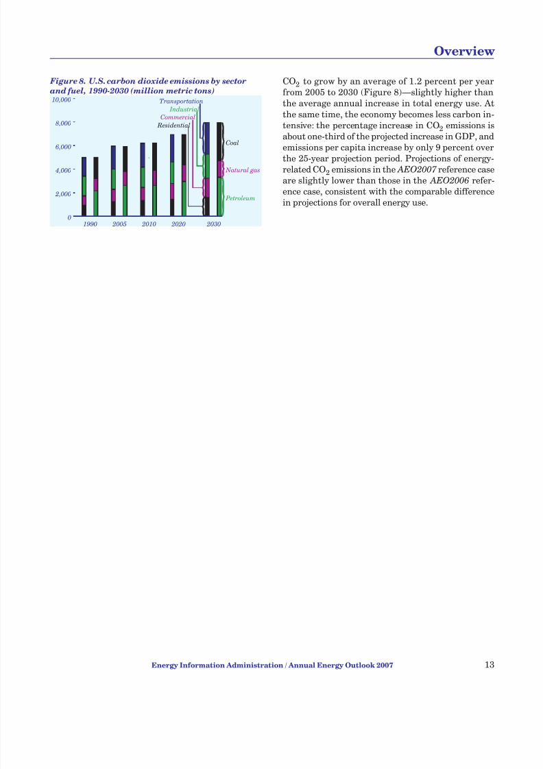
7/28/2019 2007 Annual Energy Outlook
http://slidepdf.com/reader/full/2007-annual-energy-outlook 22/243
CO2 to grow by an average of 1.2 percent per yearfrom 2005 to 2030 (Figure 8)—slightly higher thanthe average annual increase in total energy use. At
the same time, the economy becomes less carbon in-tensive: the percentage increase in CO2 emissions is
about one-third of the projected increase in GDP, andemissions per capita increase by only 9 percent overthe 25-year projection period. Projections of energy-related CO2 emissions in the AEO2007 reference caseare slightly lower than those in the AEO2006 refer-ence case, consistent with the comparable differencein projections for overall energy use.
Energy Information Administration / Annual Energy Outlook 2007 13
Overview
1990 2005 2010 2020 20300
2,000
4,000
6,000
8,000
10,000
Industrial
Commercial
Residential
Transportation
Natural gas
Coal
Petroleum
Figure 8. U.S. carbon dioxide emissions by sector
and fuel, 1990-2030 (million metric tons)

7/28/2019 2007 Annual Energy Outlook
http://slidepdf.com/reader/full/2007-annual-energy-outlook 23/243
14 Energy Information Administration / Annual Energy Outlook 2007
Overview
Table 1. Total energy supply and disposition in the AEO2007 and AEO2006 reference cases, 2005-2030
Energy and economic factors 2005
2010 2020 2030
AEO2007 AEO2006 AEO2007 AEO2006 AEO2007 AEO2006
Primary energy production (quadrillion Btu)
Petroleum . . . . . . . . . . . . . . . . . . . . . . . . . . . . . . . . . . . . . . 13.30 14.42 14.83 14.85 14.41 13.71 12.25
Dry natural gas . . . . . . . . . . . . . . . . . . . . . . . . . . . . . . . . . . 18.77 19.93 19.13 21.41 22.09 21.15 21.45
Coal . . . . . . . . . . . . . . . . . . . . . . . . . . . . . . . . . . . . . . . . . . 23.20 24.47 25.78 26.61 27.30 33.52 34.10
Nuclear power . . . . . . . . . . . . . . . . . . . . . . . . . . . . . . . . . . 8.13 8.23 8.44 9.23 9.09 9.33 9.09
Hydropower . . . . . . . . . . . . . . . . . . . . . . . . . . . . . . . . . . . . 2.71 3.02 3.03 3.08 3.04 3.09 3.04
Biomass . . . . . . . . . . . . . . . . . . . . . . . . . . . . . . . . . . . . . . . 2.71 4.22 3.90 4.69 4.66 5.26 5.07
Other renewable energy . . . . . . . . . . . . . . . . . . . . . . . . . . . 0.76 1.18 1.27 1.33 1.92 1.44 2.61
Other . . . . . . . . . . . . . . . . . . . . . . . . . . . . . . . . . . . . . . . . . 0.22 0.67 0.97 0.89 1.22 1.12 1.39
Total . . . . . . . . . . . . . . . . . . . . . . . . . . . . . . . . . . . . . . . . . 69.80 76.13 77.36 82.09 83.73 88.63 89.00
Net imports (quadrillion Btu)
Petroleum . . . . . . . . . . . . . . . . . . . . . . . . . . . . . . . . . . . . . . 26.94 25.19 26.25 28.92 30.46 34.74 36.56
Natural gas . . . . . . . . . . . . . . . . . . . . . . . . . . . . . . . . . . . . . 3.67 4.67 4.45 5.48 5.15 5.59 5.72
Coal/other (- indicates export) . . . . . . . . . . . . . . . . . . . . . . -0.42 -0.19 -0.58 0.93 0.90 1.57 2.02
Total . . . . . . . . . . . . . . . . . . . . . . . . . . . . . . . . . . . . . . . . . 30.19 29.66 30.12 35.33 36.50 41.90 44.30
Consumption (quadrillion Btu)
Liquid fuels . . . . . . . . . . . . . . . . . . . . . . . . . . . . . . . . . . . . . 40.61 41.76 43.14 46.52 48.15 52.17 53.59Natural gas . . . . . . . . . . . . . . . . . . . . . . . . . . . . . . . . . . . . . 22.63 24.73 24.04 27.04 27.70 26.89 27.65
Coal . . . . . . . . . . . . . . . . . . . . . . . . . . . . . . . . . . . . . . . . . . 22.87 24.24 25.09 27.29 27.65 34.14 34.49
Nuclear power . . . . . . . . . . . . . . . . . . . . . . . . . . . . . . . . . . 8.13 8.23 8.44 9.23 9.09 9.33 9.09
Hydropower . . . . . . . . . . . . . . . . . . . . . . . . . . . . . . . . . . . . 2.71 3.02 3.03 3.08 3.04 3.09 3.04
Biomass . . . . . . . . . . . . . . . . . . . . . . . . . . . . . . . . . . . . . . . 2.38 3.30 3.25 3.64 3.73 4.06 4.09
Other renewable energy . . . . . . . . . . . . . . . . . . . . . . . . . . . 0.76 1.18 1.27 1.33 1.92 1.44 2.61
Net electricity imports . . . . . . . . . . . . . . . . . . . . . . . . . . . . . 0.08 0.04 0.07 0.04 0.05 0.04 0.05
Total. . . . . . . . . . . . . . . . . . . . . . . . . . . . . . . . . . . . . . . . . 100.19 106.50 108.34 118.16 121.32 131.16 134.60
Liquid fuels (million barrels per day)
Domestic crude oil production . . . . . . . . . . . . . . . . . . . . . . 5.18 5.67 5.88 5.89 5.55 5.39 4.57
Other domestic production . . . . . . . . . . . . . . . . . . . . . . . . . 3.04 4.03 3.98 4.49 4.87 5.08 5.82
Net imports . . . . . . . . . . . . . . . . . . . . . . . . . . . . . . . . . . . . . 12.57 11.79 12.36 13.56 14.47 16.37 17.29
Consumption . . . . . . . . . . . . . . . . . . . . . . . . . . . . . . . . . . . 20.75 21.59 22.18 24.03 24.82 26.95 27.57
Natural gas (trillion cubic feet)
Production . . . . . . . . . . . . . . . . . . . . . . . . . . . . . . . . . . . . . 18.30 19.42 18.65 20.86 21.52 20.61 20.90
Net imports . . . . . . . . . . . . . . . . . . . . . . . . . . . . . . . . . . . . . 3.57 4.55 4.35 5.35 5.02 5.45 5.57
Consumption . . . . . . . . . . . . . . . . . . . . . . . . . . . . . . . . . . . 21.98 24.02 23.35 26.26 26.92 26.12 26.86
Coal (million short tons)
Production . . . . . . . . . . . . . . . . . . . . . . . . . . . . . . . . . . . . . 1,131 1,189 1,261 1,323 1,355 1,691 1,703
Net imports . . . . . . . . . . . . . . . . . . . . . . . . . . . . . . . . . . . . . -21 -7 -26 41 36 68 83
Consumption . . . . . . . . . . . . . . . . . . . . . . . . . . . . . . . . . . . 1,128 1,195 1,233 1,377 1,390 1,772 1,784
Prices (2005 dollars)
Imported low-sulfur, light crude oil (dollars per barrel ) . . . . 56.76 57.47 48.50 52.04 52.00 59.12 58.42
Imported crude oil (doll ars per barrel) . . . . . . . . . . . . . . . . 49.19 51.20 45.12 46.47 46.14 51.63 51.27
Domestic natural gas at wellhead(dollars per thousand cubic feet) . . . . . . . . . . . . . . . . . . . . 7.51 5.76 5.15 5.22 5.02 5.98 6.07
Domestic coal at minemouth (dollars per short ton) . . . . . . 23.34 24.20 22.80 21.58 20.72 22.60 22.29
Average electricity price (cents per kilowatthour). . . . . . . . 8.1 8.1 7.5 7.9 7.4 8.1 7.7
Economic indicatorsReal gross domestic product (billion 2000 dollars). . . . . . . 11,049 12,790 13,043 17,077 17,541 22,494 23,112
GDP chain-type price index (i ndex, 2000=1.000). . . . . . . . 1.127 1.253 1.235 1.495 1.597 1.815 2.048
Real disposable personal income (bil lion 2000 dollars) . . . 8,105 9,568 9,622 13,000 13,057 17,535 17,562
Value of manufacturing shipments (billion 2000 doll ars) . . 5,763 6,298 6,355 7,779 7,778 9,502 9,578
Primary energy intensity(thousand Btu per 2000 dollar of GDP) . . . . . . . . . . . . . . 9.07 8.33 8.31 6.92 6.92 5.83 5.82
Carbon dioxid e emissions (million metric tons) . . . . . . . 5,945 6,214 6,365 6,944 7,119 7,950 8,114
Notes: Quantities are derived from historical volumes and assumed thermal conversion factors. Other production includes liquid hydrogen,methanol, and some inputs to refineries. Net imports of petroleum include crude oil, petroleum products, unfinished oils, alcohols, ethers, andblending components. Other net imports include coal coke and electricity.
Sources: AEO2007 National Energy Modeling System, run AEO2007.D112106A; and AEO2006 National Energy Modeling System, run AEO2006.D111905A.

7/28/2019 2007 Annual Energy Outlook
http://slidepdf.com/reader/full/2007-annual-energy-outlook 24/243
Legislation andRegulations

7/28/2019 2007 Annual Energy Outlook
http://slidepdf.com/reader/full/2007-annual-energy-outlook 25/243
Introduction
Because analyses by EIA are required to be policy-neutral, the projections in AEO2007 generally arebased on Federal and State laws and regulations in
effect on or before October 31, 2006 (although thereare exceptions to this rule, as discussed below). The
potential impacts of pending or proposed legis-
lation, regulations, and standards—or of sec-
tions of legislation that have been enacted but
that require implementing regulations or ap-
propriation of funds that are not provided or
specified in the legislation itself—are not re-
flected in the projections.
Selected examples of Federal and State legislation in-corporated in the projections include the following:
The new CAFE standards finalized in March2006, which establish higher minimum fuel econ-omy performance requirements by vehicle foot-print for light-duty trucks
• EPACT2005, which includes mandatory energyconservation standards; creates numerous taxcredits for businesses and individuals; creates anRFS and eliminates the oxygen content require-ment; extends royalty relief for offshore oil andnatural gas producers; and extends and expandsthe PTC for electricity generated from renewablefuels
• The Military Construction Appropriations Actof 2005, which contains provisions to supportconstruction of the Alaska natural gas pipeline,including Federal loan guarantees during con-struction
• The Working Families Tax Relief Act of 2004,which includes tax deductions for qualified clean-fuel and electric vehicles; and changes in the rulesgoverning oil and natural gas well depletion
• The American Jobs Creation Act of 2004, whichincludes incentives and tax credits for biodiesel
fuels and a modified depreciation schedule for the Alaska natural gas pipeline
• The Maritime Security Act of 2002, whichamended the Deepwater Port Act of 1974 to in-clude offshore natural gas facilities
• State RPS programs, including the California RPS passed on September 12, 2002
• The Clean Air Act Amendments of 1990 (CAAA-90), which included new standards for motor
gasoline and diesel fuel and for heavy-duty vehicleemissions
• The National Appliance Energy Conservation Actof 1987
• State programs for restructuring of the electricityindustry.
AEO2007 assumes that State taxes on gasoline, die-sel, jet fuel, and E85 [ 4] will increase with inflationand that Federal taxes on those fuels will remain atthe nominal rate established in 2003 (the last timethe Federal taxes were changed). AEO2007 also as-sumes that the ethanol tax credit, as modified underthe American Jobs Creation Act of 2004, will be ex-tended when it expires in 2010 and will remain in
force indefinitely. Although the ethanol tax credit
includes a “sunset” clause that limits its duration,historically it has been extended regularly, and AEO-
2007 assumes its continuation throughout the pro- jection [5 ]. AEO2007 also includes the biodiesel taxcredits that were created under the American JobsCreation Act and extended through 2008 underEPACT2005; however, they are not assumed to be ex-tended further, because they have minimal history of
legislative extension.
The Safe, Accountable, Flexible, Efficient Transpor-
tation Equity Act: A Legacy for Users (SAFETEA-LU) increased the Federal tax on compressed natural
gas used in vehicles to 18.3 cents per equivalent gal-lon of gasoline and provided a credit of 50 cents pergallon through September 2009. AEO2007 assumesthat State and Federal taxes on compressed naturalgas for vehicles will continue at 2006 levels in nomi-nal terms and that the tax credit will not be extended.
The PTC for wind, geothermal, landfill gas (LFG),and some types of hydroelectric and biomass-fueledplants, established initially by the Energy Policy Actof 1992 [6] also is represented in AEO2007 . Only new
plants that come on line before January 1, 2008, are
eligible to receive the credit. AEO2007 does not as-sume extension of the PTC, whichhas been allowed toexpire in the past, even though it has typically beenrenewed retroactively. In most of the extensions, thecredit has been modified significantly: additional re-sources have been included, resources previously eli-gible have been excluded, and the structure and
treatment of the credit itself have been changed.
Selected examples of Federal and State regulationsincorporated in AEO2007 include the following:
16 Energy Information Administration / Annual Energy Outlook 2007
Legislation and Regulations

7/28/2019 2007 Annual Energy Outlook
http://slidepdf.com/reader/full/2007-annual-energy-outlook 26/243
• New stationary diesel regulations issued by theU.S. Environmental Protection Agency (EPA) on
July 11, 2006, which limit emissions of NOx,
particulate matter, SO2, carbon monoxide, andhydrocarbons to the same levels required by the
EPA’s nonroad diesel engine regulations
• The Clean Air Interstate Rule (CAIR) and Clean Air Mercury Rule (CAMR), promulgated by the
EPA in March 2005 and published in the Federal
Register as final rules in May 2005, which willlimit emissions of SO2, NOx, and mercury frompower plants in the United States
• New boiler limits established by the EPA on Feb-ruary 26, 2004, which limit emissions of hazard-ous air pollutants from industrial, commercial,and institutional boilers and process heaters by
requiring that they comply with a Maximum Achievable Control Technology floor.
AEO2007 does not include consideration of California Assembly Bill (A.B.) 32 (discussed below), whichmandates a 25-percent reduction in California’sgreenhouse gas emissions by 2020. Implementing regulations have not been drafted and are not due tobe finalized until January 2012.
In addition, California’s A.B. 1493, which establishesgreenhouse gas emissions standards for light-duty ve-hicles, is not considered in the AEO2007 referencecase. A.B. 1493 was signed into law in July 2002, and
regulations were released by the California Air Re-sources Board in August 2004 and approved by Cali-fornia’s Office of Administrative Law in September2005; however, the automotive industry has filed suitto block their implementation, and the Board has not
yet obtained a Clean Air Act waiver from the EPA,which is required before the regulations can beimplemented.
In August 2006, seven northeastern States released a model rule for implementation of the Regional Green-house Gas Initiative (RGGI) [7 ], as discussed below,
clarifying what had been laid out in December 2005when the States entered into the agreement [8]. TheRGGI, which would cap greenhouse gas emissionsfrom power producers, requires each State to enactlegislation for accomplishing the emissions reduc-tions. Although the State RGGI caps and timelinesare known, many aspects of their implementation re-main uncertain, because the participating Stateshave not yet enacted the necessary legislation. There-fore, the RGGI provisions are not modeled in the
AEO2007 reference case.
AEO2007 does include the CAAA90 requirement of a phased-in reduction in vehicle emissions of regulatedpollutants. It also reflects “Tier 2” Motor Vehicle
Emissions Standards and Gasoline Sulfur Control Re-quirements finalized by the EPA in February 2000
under CAAA90. The Tier 2 standards for reformu-lated gasoline (RFG) were required by 2004, but be-cause they included allowances for small refineries,they will not be fully realized for conventional gaso-line until 2008. AEO2007 also incorporates the ul-tra-low-sulfur diesel fuel (ULSD) regulation finalizedby the EPA in December 2000, which requires the
production of at least 80 percent ULSD (less than orequal to 15 parts sulfur per million) highway dieselbetween June 2006 and June 2010 and 100 percentULSD thereafter. It also includes the rules fornonroad diesel issued by the EPA on May 11, 2004,
regulating nonroad diesel engine emissions and sul-fur content in fuel.
More detailed information on recent and proposedlegislative and regulatory developments is providedbelow.
EPACT2005: Status of Provisions
EPACT2005 was signed into law by President Bushon August 8, 2005, and became Public Law 109-058[9]. A number of provisions from EPACT2005 wereincluded in the AEO2006 projections [10]. Many oth-
ers were not considered in AEO2006—particularly,those that require funding appropriations or furtherspecification by Federal agencies or Congress beforeimplementation.
A number of the EPACT2005 provisions not includedin AEO2006 could affect the projections. In the prepa-
ration of AEO2007 their status was reviewed, andwhere possible, additional provisions were includedin the projections; however, AEO2007 still excludesthose EPACT2005 provisions whose impacts arehighly uncertain or that address a level of detail be-
yond that modeled in NEMS. Furthermore, EIA does
not try to anticipate policy responses to the manystudies required by EPACT2005 nor predict the im-pacts of research and development (R&D) funding au-
thorizations included in the bill.
The following summary examines the status of EPACT2005 provisions that initially could not be in-cluded in AEO2006 but potentially could be modeledin NEMS. It focuses on provisions that are newly in-cluded in AEO2007 , as well as those that might be
added in future AEOs. The discussion below does not
Energy Information Administration / Annual Energy Outlook 2007 17
Legislation and Regulations
7/28/2019 2007 Annual Energy Outlook
http://slidepdf.com/reader/full/2007-annual-energy-outlook 27/243
provide a complete summary of all the sections of
EPACT2005. More extensive summaries are avail-
able from other sources [11].
End-Use Demand Provisions
This section summarizes provisions of EPACT2005that affect the end-use demand sectors.
Buildings
EPACT2005 includes provisions with the potential to
affect energy demand in the residential and commer-
cial buildings sector. Many are included in Title I,
“Energy Efficiency.” Others can be found in the re-
newable energy, R&D, and tax titles. Most of the
provisions that have been funded or for which imple-
menting regulations have been put in place since the
publication of AEO2006, cannot be modeled in
NEMS. The status of those provisions that could po-tentially be included in NEMS is summarized below.
Section 122 of Title I, “Weatherization Assistance,”
authorizes $600 million to weatherize low-income
households. The weatherization program, in exis-
tence since 1976, uses Federal funds to increase the
energy efficiency of low-income houses. In fiscal year
(FY) 2006, funding for this program was $242 million.
FY 2007 funding proposed by the U.S. House of Rep-
resentatives is set at $250 million. The increase in
funding could allow up to 3,200 more homes to be
weatherized in FY 2007 than in FY 2006. TheAEO-
2007 reference case includes increases in energy effi-
ciency in existing building envelopes to account for
programs such as weatherization. At current funding
levels, roughly 100,000 homes are weatherized each
year. The impact of this section is considered in
AEO2007 .
Section 204 of Title II, “Use of Photovoltaic Energy in
Public Buildings,” authorizes funds for the establish-
ment of a photovoltaic (PV) energy commercializa-
tion program to procure, install, and evaluate PV
solar electric systems in public buildings. No funding
has been appropriated to date for this measure. It isnot included in AEO2007 .
Section 206 of Title II, “Renewable Energy Security,”
authorizes funds for the establishment of rebates for
the purchase of renewable energy systems, including
PV, ground-source heat pumps, and solar water heat-
ers. This program was to be in place starting in calen-
dar year 2006 and last through 2010; however, no
funding has been appropriated for the measure to
date, and it is not included in AEO2007 .
Section 783 of Title VII, “Federal Procurement of
Stationary, Portable, and Micro Fuel Cells,” autho-
rizes funds for Federal procurement of stationary,
portable, and micro fuel cells. No funding has been
appropriated for the measure to date, and it is not
considered in AEO2007 .
Industrial
EPACT2005 includes few provisions that would spe-
cifically affect industrial sector energy demand. Pro-
visions in the R&D titles that may affect industrial
energy consumption over the long term are not in-
cluded in AEO2007 .
Section 108 requires that federally funded projects in-
volving cement or concrete increase the amount of re-
covered mineral component (e.g., fly ash or blast
furnace slag) used in the cement. Such use of mineralcomponents is a standard industry practice, and in-
creasing the amount could reduce both the quantity
of energy used for cement clinker production and the
level of process-related CO2 emissions. The propor-
tion of mineral component is not specified in the
legislation but is to be determined by Federal pro-
curement rules; however, as of mid-September 2006
the rules had not been promulgated. Section 108 also
requires that the energy-saving impact of the rules be
assessed by the EPA, in cooperation with the U.S. De-
partment of Energy (DOE) and Department of Trans-
portation (DOT), within 30 months of enactment.
Because regulations have not been promulgated, this
section is not considered in AEO2007 . When the regu-
lations are promulgated, their estimated impacts
could be modeled in NEMS.
Section 1321 provides for the extension of tax credits
for producers of coke or coke gas, effective for tax
years beginning after December 31, 2005. Otherwise,
the status of Section 1321 is unchanged. Because the
bulk of the credits will go to plants already operating
or under construction, there is likely to be little im-
pact on coke plant capacity. Consequently, the provi-
sion is expected to have no impact on the AEO2007 projections.
Coal Gasification Provisions
This section provides updates to the funding and im-
plementation status of key tax incentive provisions in
Title XIII of EPACT2005 related to coal gasification
that were not addressed in AEO2006.
Section 1307 creates an investment tax credit pro-
gram for qualifying advanced clean coal projects,
18 Energy Information Administration / Annual Energy Outlook 2007
Legislation and Regulations

7/28/2019 2007 Annual Energy Outlook
http://slidepdf.com/reader/full/2007-annual-energy-outlook 28/243
funded at $1.3 billion. The section also includes an ad-ditional $350 million for qualifying gasification pro-
jects. The gasification credit for any taxable year is
equal to 20 percent of the basis of any equipment to beused in the gasification process that is placed in ser-
vice during the year as part of a gasification projectthat has been certified by DOE as eligible for thecredit. The amount eligible for credit is limited to$650 million per project. Only domestic projects thatemploy domestic gasification applications are eligible.
Applicants must, among other criteria, satisfy certainfinancial requirements, prove that a market exists for
the project’s products, and demonstrate competencyin the development and operation of the project.Credits are not allowed for gasification projects re-ceiving credits under the program for advanced coalprojects. A certificate of eligibility is valid for 10 fiscal
years, beginning on October 1, 2005.
In February 2006, the IRS issued guidance for theSection 1307 program. Certifications are to be issuedand credits allocated to projects in annual allocationrounds. The first round of submissions began on Feb-ruary 21, 2005, and closed on October 2, 2006. Over-all, the period for submission of applications is to runfor 3 years, starting on February 21, 2006. As of Au-gust 2006, 49 applications had been received, 27 of
which fell under the gasification technology programand were for CTL plants in 17 States. The 27 projectsare valued at $30 billion and request tax credits of $2.7 billion. Selection of projects to receive the creditsis scheduled for the end of November 2006.
Credits will be allocated first to projects that have
CO2 capture capability, use renewable fuel, or haveproject teams with experience that demonstrates suc-cessful operation of the gasification technology. If therequested allocations exceed $350 million, the creditswill be allocated to the projects that provide the high-est ratio of synthetic gas supplied to the requested al-location of credits. Any remaining credits will beapplied to non-priority projects that provide the high-
est amount of nameplate capacity. If funds remain inthe program, additional rounds will be conducted in2007 and 2008. The $1.3 billion in tax credits for theadvanced clean coal program was accounted for in AEO2006 in the NEMS Electricity Market Module.CTL projects are eligible for the gasification credits,because gasification is the first step in the CTL pro-cess; however, because the level of interest in coalgasification projects was not known at the time, the
gasification program credits were not included in
AEO2006. Given the extent of interest in the programto date, they are included in the Electricity MarketModule for AEO2007 .
Oil and Natural Gas Provisions
This section provides updates to the funding and im-plementation status of key oil and natural gas provi-sions of EPACT2005 that were not addressed in
AEO2006. Most of the oil and natural gas provisionsin EPACT2005 are included in Title III, “Oil andGas.” Others, covering R&D, are included in Title IX.
The Federal Energy Regulatory Commission (FERC)was authorized by Section 312 to allow natural gasstorage facilities to charge market-based rates if itwas believed that they would not exert market power.On June 15, 2006, FERC finalized rules implement-
ing the provisions that would allow an applicant forinterstate natural gas storage facilities to request au-thority to charge market-based rates even if a lack of market power had not been demonstrated. The rulesare intended to mitigate natural gas price volatility byencouraging the development of new natural gas stor-age capacity. They apply in circumstances where mar-ket-based rates are in the public interest andnecessary to encourage the construction of storage ca-pacity and to ensure that customers are adequately
protected, even in circumstances where marketpower may not have been demonstrated. In previous AEO
s, storage rates were allowed to vary from regula-tion-based rates, depending on market conditions.
In compliance with Section 354, DOE established a competitive program to provide grants for cost-shared projects to enhance oil and natural gas recov-ery through CO2 injection, while at the same time se-questering CO2 produced from the combustion of
fossil fuels in power plants and large industrial pro-cesses. Reports issued by DOE indicate that an addi-tional 89 billion barrels of oil could be recovered in theUnited States through CO2 injection. Under the pro-gram, grants of up to $3 million will be provided to
each project selected. On September 6, 2006, DOE an-nounced the selection of the first project to receiveone of the grants, a project sponsored by the Univer-sity of Alabama-Birmingham to implement a demon-
stration project in the Citronelle oilfield in MobileCounty, AL. The total project cost is estimated at$6 million, with DOE’s maximum share at just under$3 million. Estimates indicate that an additional64 million barrels of oil could be recovered from theCitronelle field by this technique.
Energy Information Administration / Annual Energy Outlook 2007 19
Legislation and Regulations

7/28/2019 2007 Annual Energy Outlook
http://slidepdf.com/reader/full/2007-annual-energy-outlook 29/243
The implementation of Section 354 was not includedin previous AEOs, because NEMS does not representproject-level activities and because of the consider-
able uncertainty surrounding the eventual scope of the program. For AEO2007 , however, additional oil
resources have been added to account for increaseduse of CO2-enhanced oil recovery technology.
Section 311 clarified the role of FERC as the finaldecisionmaking body on any issues concerning on-shore facilities that export, import, or process LNG.On October 7, 2005, FERC established mandatoryprocedures requiring prospective applicants for LNG
terminals, related jurisdictional pipelines, and otherrelated natural gas facilities to begin the Commis-sion’s pre-filing review process at least 6 months be-fore filing an application to site and/or construct such
a facility. The procedures, which also apply to applica-tions for modifications of existing or authorized LNGterminals, are designed to encourage applicants to co-operate with State and local officials.
In March 2005 and June 2006, FERC and DOE, in co-
operation with DOT and the U.S. Department of Homeland Security, conducted three public forumson LNG designed to promote public education andencourage cooperation between State and Federalofficials in areas where LNG terminals are being con-sidered for construction. They were held in Boston,MA; Astoria, OR; and Los Angeles, CA. An additional
forum is planned for Houston, TX, in the 4th quarterof 2006, fully satisfying the Section 317 requirement
that a minimum of three such forums be held. Al-though this provision is not explicitly represented inthe AEO2007 NEMS, the model includes an assump-tion that there are no major regulatory impedimentsto the siting of new LNG facilities.
Section 301 authorized DOE to increase the capacityof the Strategic Petroleum Reserve (SPR) to 1 billionbarrels from its current capacity of 727 million bar-rels. DOE has announced plans to add additional stor-
age capacity to its SPR storage sites in Big Hill, TX;Bayou Choctaw, LA; West Hackberry, LA; and onenew site in Richton, MS. DOE filed a draft site selec-tion Environmental Impact Statement with the EPA on May 19, 2006, for the selection of a new site,and comments have been received. In order for theadditional storage capacity to be authorized, con-structed, and ultimately filled, further actions byCongress and the Executive Branch will be required;
therefore, it is not considered in AEO2007 .
Section 369 requires DOE to initiate a process for theleasing of Federal lands for research on oil shale, tarsands, and other unconventional fuels. Several indus-
try research proposals were evaluated, and on Janu-ary 17, 2006, the U.S. Department of the Interior’s
Bureau of Land Management announced the selec-tion of six applicants for oil shale leases to receive fur-ther consideration. Because the lease applications arestill under consideration, this provision is not ac-counted for in AEO2007 .
Coal Provisions
This section provides updates to the funding and im-plementation status of provisions in EPACT2005 that
will affect coal supply and prices but were not ad-dressed in AEO2006. Many of the provisions can befound in Titles IV and XIII of EPACT2005.
A number of coal-related provisions that were autho-rized by EPACT2005 but not included in AEO2006
continue to be excluded from AEO2007 . They includefour loan guarantee or cost-sharing programs. Sec-tion 411 authorized a loan guarantee for a coal projectin the Upper Great Plains, which must employ bothrenewable and advanced IGCC technologies. A loanguarantee for the Clean Coal Project in Healy, AK,
authorized by Section 412, also is excluded from AEO2007 . In Section 413, EPACT2005 authorized a cost-sharing program in support of a high-altitude (at
least 4,000 feet) Western IGCC Demonstration Pro- ject. Finally, a loan guarantee for an IGCC plantlocated in a deregulated region was authorized bySection 414.
These provisions have spurred some activity and in-terest. For instance, Xcel Energy, which has proposedbuilding a facility in Colorado with 300 to 350 mega-watts of generating capacity, is a potential applicantfor the Western IGCC Demonstration Project. On Au-gust 7, 2006, DOE released its plans to form a pro-gram office with functions that include the drafting of application guidelines for the various loan programs.
It will also be charged with the task of awarding theloan guarantees. Although NEMS has the capabilityto represent these coal provisions, Congress had notappropriated funds for the provisions as of September1, 2006, and they are not considered in AEO2007 .
Nuclear Energy Provisions
EPACT2005 includes numerous provisions that ad-dress nuclear power generation. This section provides
20 Energy Information Administration / Annual Energy Outlook 2007
Legislation and Regulations

7/28/2019 2007 Annual Energy Outlook
http://slidepdf.com/reader/full/2007-annual-energy-outlook 30/243
updates to the funding and implementation status of nuclear power generation provisions in EPACT2005that were not addressed in AEO2006.
Section 1306 of Title 13 extends the PTC of 1.8 cents
per kilowatthour (not adjusted for inflation) to anynuclear power plant with a “new” design that has a construction start date before January 1, 2014, andenters commercial operation by January 1, 2021. Un-der this program, the owner of the eligible plant can
reduce its tax liability by up to 1.8 cents for eachkilowatthour of plant output. For the purposes of thislaw, construction begins when a utility “that has ap-plied for or been granted a combined operating li-cense . . . initiates the pouring of safety-relatedconcrete for the reactor building.” The IRS publishedan initial set of guidelines for the program in May
2006 and eventually will publish a set of formal rulesthat will become part of the Tax Code. In EPACT-
2005, the per-kilowatthour tax credit was indexed tothe rate of inflation; however, the indexing provisionwas eliminated in the Gulf Opportunity Zone Act of 2005 (P.L. 109-135). Consequently, the credit wouldbe constant in nominal dollars over time. Because theearliest date at which the first new nuclear unit eligi-ble for the tax credit could become operational isabout 2015, the “de-indexing” of the credit has the ef-
fect of reducing its real value by about 25 to 30percent.
There are at least three limitations on the amount of tax credits a utility can receive. First, tax credits inany given year are limited to a maximum of $125 perkilowatt ($125 million for a 1,000-megawatt unit).
Second, the tax credit can be applied only in the first 8 years of a plant’s operation. Third, the credit is lim-ited to a maximum of 6 gigawatts of new nuclear ca-pacity nationally. If the total capacity qualifying forthe tax credit exceeds 6 gigawatts, the amount of thecredit per kilowatthour will be reduced proportion-ally. AEO2007 assumes that up to 9 gigawatts of newcapacity will receive the Title 13 PTC at 1.2 cents per
kilowatthour. ( AEO2006 assumed that 6 gigawattswould receive the full 1.8 cents per kilowatthour.) AEO2007 also assumes that participating utilitieswill be able to take all the tax credits in each of thefirst 8 years of their qualifying units’ operation.
Title 17 of EPACT2005 allows the Governmentto guarantee loans used to construct new energy tech-
nologies “that reduce or avoid greenhouse gases,” in-cluding new nuclear power plants. The Secretary of Energy can guarantee a loan of upto 80 percent of the
project’s cost; however, DOE will not guarantee morethan 80 percent of the total debt. Thus, if a utility de-cided to fund a project with 80 percent debt and 20
percent equity, DOE would only guarantee up to 64percent of the project’s total cost. Such loan guaran-
tees would affect the economics of nuclear power, be-cause they would reduce the effective interest rateson the debt and allow utilities to use much more debtfinancing.
The Secretary of Energy will choose the projects thatwill receive the loan guarantees. The factors to beconsidered in the selection of projects include:
• A relatively low probability of failure
• The extent to which the project avoids, reduces, orsequesters air pollutants or emissions of green-house gases
• The extent to which the project will advance thegoals of the President’s Advanced Energy Initia-tive
• The extent to which the technology is ready to beemployed commercially in the United States andcan yield a commercially viable product.
Because of the lack of appropriating legislation, thisprogram is not included in AEO2007 .
Fuel Economy Standards for New LightTrucks
In March 2006, NHTSA finalized CAFE standards re-quiring higher fuel economy performance for light-duty trucks in MY 2008 through 2011 [12]. Unlike theproposed CAFE standards discussed in AEO2006
[13], which would have established minimum fueleconomy requirements by six footprint size classes,the final reformed CAFE standards specify a continu-
ous mathematical function that determines mini-mum fuel economy requirements by vehicle footprint,defined as the wheelbase (the distance from the frontaxle to the center of the rear axle) times the averagetrack width (the distance between the center lines of
the tires) of the vehicle in square feet.
As shown in Figure 9, the new fuel economy stan-dards vary by model year (MY) and by vehicle foot-print. By eliminating the categories laid out in theproposed rule, the final rule removes the opportunityfor manufacturers to reduce fuel economy require-ments by altering vehicle sizes just enough to reachlower target levels. Instead, under a continuous func-tion approach, each footprint value has an assigned
fuel economy target, and small changes in vehicle
Energy Information Administration / Annual Energy Outlook 2007 21
Legislation and Regulations

7/28/2019 2007 Annual Energy Outlook
http://slidepdf.com/reader/full/2007-annual-energy-outlook 31/243
footprint are not rewarded with large decreases intarget values.
In addition to reforming the structure of the lighttruck CAFE program, NHTSA has also increased the
gross vehicle weight rating (GVWR) of light truckscovered under CAFE. NHTSA defines light-dutytrucks as trucks with a GVWR of 10,000 pounds orless, including pickups, vans, truck-based stationwagons, and sport utility vehicles (SUVs). Current
CAFE standards apply to light-duty trucks that havea GVWR of 8,500 pounds or less.
Starting in MY 2011, light truck CAFE standards willalso apply to medium-duty passenger vehicles(MDPVs), which are defined as complete heavy-dutyvehicles less than 10,000 pounds GVWR that are de-
signed primarily for transportation of passengers.The definition of an MDPV does not include vehiclessold as incomplete trucks (i.e., a truck cab on chassis);vehicles that have a seating capacity of more than 12persons; vehicles designed for more than 9 persons inseating rearward of the driver’s seat; or vehiclesequipped with an open cargo area (e.g., a pickup truckbox or bed) of 6 feet or more in interior length. Hence,the definition of an MDPV essentially includes SUVs,
short-bed pickup trucks, and passenger vans that arewithin the specified weight and weight-rated ranges.This implies that, starting in MY 2011, all SUVsgreater than 8,500 GVWR that are currently excluded
from CAFE consideration and all passenger vansless than 10,000 pounds GVWR will be included indetermining a manufacturer’s light truck CAFEcompliance.
To provide manufacturers adequate time to adjusttheir product plans to the new provision, NHTSA is
making the new definition effective beginning in MY 2011. As a result, the change will not have an immedi-ate impact on MY 2008-2010 vehicles. In addition,
NHTSA is permitting manufacturers to rely on eitherthe old or the revised definition of light trucks until
MY 2011.
NHTSA has also amended the “flat floor provision” to
include only vehicles that have at least three rows of seats, of which the second and third rows can be de-tached or folded to create a flat cargo surface. Manu-facturers currently offering minivans with folding seats will be able to take advantage of the new defini-tion immediately. The new CAFE standards continueto exclude most medium- and heavy-duty pickups andmost medium- and heavy-duty cargo vans that areused primarily for agricultural and commercial pur-poses. The change in the definition of a light truckcan also have an impact on the product mix that a manufacturer will offer, because some light trucksunder the current definition could be categorized ascars under the new definition, with a higher CAFErequirement.
The reformed CAFE standards impose a unique fueleconomy standard on each manufacturer, based onthe product mix sold in a given MY. For MY 2008through 2010, manufacturers have the option of com-plying with either the new reformed CAFE standardor an unreformed CAFE standard. The unreformed
CAFE standard requires manufacturers to meet anaverage light truck fleet standard of 22.5 miles pergallon in MY 2008, 23.1 miles per gallon in MY 2009,and 23.5 miles per gallon in MY 2010. All light truckmanufacturers must adhere to the new reformedstandards for MY 2011 and subsequent years.
Each manufacturer is subject to an identical fueleconomy target for light truck models with the samefootprint. Moreover, the same formula is applied todetermine each manufacturer’s required CAFE level,using the fuel economy targets for different foot-prints, the targets specific for each model, and the
production levels of each model. Individual manufac-turers face different required CAFE levels only to theextent that they produce different volumes of vehiclesby footprint.
To determine compliance with the reformed CAFEstandard, each manufacturer’s production-weightedaverage fuel economy will be calculated and comparedto the calculated reformed CAFE. If the weighted av-erage fuel economy of all the manufacturer’s modelsis at least equal to the manufacturer’s calculated
22 Energy Information Administration / Annual Energy Outlook 2007
Legislation and Regulations
35 40 45 50 55 60 65 70 75 780
10
20
30
MY 2010 MY 2011
MY 2009 MY 2008
Vehicle footprint
C A F E s t a n d a r d
Figure 9. Reformed CAFE standards (miles per
gallon) for light trucks, by model year and vehicle
footprint (square feet)

7/28/2019 2007 Annual Energy Outlook
http://slidepdf.com/reader/full/2007-annual-energy-outlook 32/243
reformed CAFE, then the manufacturer will be incompliance with the reformed CAFE standard. If itsactual fleet-wide average fuel economy is greater than
its required CAFE level, the manufacturer will earncredits equal to the difference, which can be applied to
any of the three preceding or subsequent model years. With this allowance, manufacturers will not be penal-ized for occasionally failing to meet the targets (due tomarket conditions, for example) but only for persis-tent failure to meet them. If the average fuel economyof a manufacturer’s annual car or truck productionfalls below the defined standard, the manufacturer
will be required to pay a penalty proportional to its to-tal production for the U.S. domestic market.
The new CAFE standards are captured in the AEO-
2007 projections. For MY 2008 through 2011, manu-facturers are assumed to adhere to the increases inunreformed light truck standards. For MY 2011, the
AEO2007 applies a fleet-wide standard of 24 miles pergallon, based loosely on the change between 2010 and2011 in the proposed footprint-based standards. Be-cause no further changes in fuel economy standardsbeyond 2011 are assumed, the projected increase inlight truck fuel economy after 2011 reflects projectedtechnology adoption resulting from other marketforces.
Regulation of Emissions from Stationary Diesel Engines
On July 11, 2006, the EPA issued regulations cover-ing emissions from stationary diesel engines [14]—New Source Performance Standards that limit emis-sions of NOx, particulate matter, SO2, carbon monox-ide, and hydrocarbons to the same levels required fornonroad diesel engines [15 ]. The regulation affects
new, modified, and reconstructed diesel engines. Be-ginning with MY 2007 [16], engine manufacturersmust specify that new engines less than 3,000 horse-power meet the same emissions standard as nonroaddiesel engines. For engines greater than 3,000 horse-power, the standard will be fully effective in 2011
[17 ]. Stationary diesel engine fuel will also be subjectto the same standard as nonroad diesel engine fuel,which reduces the sulfur content of the fuel to 500
parts per million by mid-2007 and 15 parts per millionby mid-2010.
Stationary diesel engines are used to generate elec-tricity, to power pumps and compressors, and inirrigation systems. It has been estimated that therewere 663,780 such engines larger than 50 horsepower
in use in 1998 [18]. The EPA estimates that 81,500
engines will be subject to the controls by 2015 andthat total pollutant reductions will be more than68,000 tons per year.
The new standards for stationary diesel engines are
included in AEO2007 , but they are unlikely to affectthe projections materially. The nonroad diesel stan-dards were incorporated in the AEO projections pre-viously, beginning with AEO2005 .
Federal and State Ethanol and BiodieselRequirements
EPACT2005 requires that the use of renewable motorfuels be increased from the 2004 level of just over 4billion gallons to a minimum of 7.5 billion gallons in2012, after which the requirement grows at a rateequal to the growth of the gasoline pool [19]. The law
does not require that every gallon of gasoline or dieselfuel be blended with renewable fuels. Refiners arefree to use renewable fuels, such as ethanol andbiodiesel, in geographic regions and fuel formulationsthat make the most sense, as long as they meet theoverall standard. Conventional gasoline and dieselcan be blended with renewables without any changeto the petroleum components, although fuels used inareas with air quality problems are likely to requireadjustment to the base gasoline or diesel fuel if they
are to be blended with renewables.
Before EPACT2005, a major portion of the RFG pool
was blended with methyl tertiary butyl ether (MTBE)to meet required oxygen levels, increase volume, im-prove octane, and maintain compatibility with exist-ing petroleum product pipelines without a large
increase in gasoline volatility. The oxygen contentwas required under CAAA90 [ 20]. Ethanol is the onlyother economically feasible oxygenate, but it is incom-patible with existing pipelines because of its affinityfor water and causes substantial increases in gasolinevolatility. Because MTBE was easier to blend andship, refiners preferred to meet oxygen requirementswith MTBE. Over the past several years, however,
various State and local governments have banned theuse of MTBE, and some have even brought lawsuitsagainst MTBE producers over concerns that spilledMTBE and gasoline containing MTBE were polluting groundwater.
In EPACT2005, Congress repealed the oxygen re-
quirement for Federal RFG but declined to prohibitdefective product claims against producers and blend-ers of MTBE. Refiners believed that the lack of an ox-
ygenate requirement would increase their liability in
Energy Information Administration / Annual Energy Outlook 2007 23
Legislation and Regulations

7/28/2019 2007 Annual Energy Outlook
http://slidepdf.com/reader/full/2007-annual-energy-outlook 33/243
future groundwater contamination cases and volun-tarily eliminated MTBE from the gasoline pool in thesummer of 2006.
Several of the largest MTBE-consuming States had
already banned the use of MTBE and switched toethanol-blended gasoline by the time EPACT2005was passed. California, New York, and Connecticutimplemented MTBE bans in 2004 [ 21]. Ethanol dis-tillers, petroleum refiners, and petroleum product
terminal operators invested in process changes andadditional tanks to accommodate the ethanol. Despitethe flexibility allowed by the EPACT2005 RFS and itsrepeal of the oxygen content requirement, refinersbegan using ethanol in all RFG in summer 2006.
Overall levels of ethanol and biodiesel use are pro-
jected to exceed the EPACT2005 requirement in all AEO2007 cases, given the projected prices for cornand crude oil, the lack of viable substitutes for MTBE,and extension of the tax credit for ethanol blending [ 22]. EPACT2005 requires the use of 250 million gal-lons per year of ethanol produced from cellulose after2013. Production of cellulosic ethanol rises only to theminimum requirement in the AEO2007 reference
case, because the projected capital costs of cellulosicethanol plants are significantly higher than those of corn ethanol plants.
An older Federal energy law has been used specifi-
cally to promote biodiesel. The Energy Policy Act of 1992 required certain vehicle fleets to purchase alter-native-fueled light vehicles, but the vehicles were notactually required to run on alternative fuels. The En-
ergy Conservation Reauthorization Act of 1998 al-lowed the purchase of 450 gallons of pure biodiesel tooffset the requirement to purchase one alterna-tive-fueled light vehicle [ 23]. In AEO2007 , biodieseldemand for Federal fleet purchase offsets is projectedto be 7.4 million gallons per year in 2012 and 8.8 mil-lion gallons per year in 2030.
Several States have their own requirements forethanol and biodiesel in their motor fuel supplies,which are reflected in AEO2007 . Minnesota, a majorproducer of ethanol, has required all gasoline tocontain at least 7.7 percent ethanol since 1997 [ 24].Hawaii requires 85 percent of its gasoline to contain10 percent ethanol, effective on April 2, 2006 [ 25 ].The intention of the law is to spur local production of ethanol from sugar, but the ethanol could also comefrom the U.S. mainland or from Brazil.
Minnesota was also the first State to require biodieselblending into diesel fuel, at 2 percent by volume [ 26].The requirement became effective in mid-2005, when
two new biodiesel plants, each with 30 million gallonsper year capacity, began operation in the State. The
law was waived several times because of quality prob-lems with the biodiesel, but it is again in effect.
Washington requires 2 percent ethanol in gasolineand 2 percent biodiesel in diesel fuel no later thanNovember 30, 2008. The requirement will increase to5 percent once the State can produce biodiesel equalto 3 percent of its diesel demand [ 27 ]. Louisiana en-
acted a requirement for 2 percent ethanol in gasolineand 2 percent biodiesel in diesel fuel, once sufficientcapacity is built in-State [ 28, 29]. Assuming thatLouisiana’s 2-percent and Washington’s 5-percentrequirements are triggered, Louisiana, Minnesota,
and Washington will require 102 million gallons of biodiesel in 2012 and 146 million gallons in 2030.
The Federal and State policies on renewable fuelshave various effects on gasoline supply and price. Thesubstitution of ethanol for MTBE in RFG reduces the
yield of gasoline and gasoline components from a given refinery configuration. In the long run, refinersare expected to make additional investments to getback some of the gasoline capacity they lost.
Because ethanol currently is economically competi-
tive as a gasoline blending component in Minnesota,
its use in that State is not dependent on the ethanolcontent requirement, which is estimated to have noadverse impact on gasoline prices. Hawaii, on theother hand, must either produce ethanol from costlysugar or ship ethanol from the U.S. mainland orBrazil. Because both options are expected to be expen-sive, it is likely that Hawaii’s program will raise gaso-line prices. The biodiesel requirements in Minnesota,
Louisiana, and Washington may increase the avail-ability of diesel fuel in the short run and are likely toincrease diesel prices after the Federal motor fuels ex-cise tax credits for blending biodiesel expire. In the
longer run, renewable fuels requirements do not af-fect the availability of gasoline and diesel fuel, be-cause refiners are expected to adjust refineryexpansion plans in light of these mandates.
Federal Fuels Taxes and Tax Credits
The AEO2007 reference case and alternative casesgenerally assume compliance with current laws andregulations affecting the energy sector. Some provi-
sions of the U.S. Tax Code are scheduled to expire, or
24 Energy Information Administration / Annual Energy Outlook 2007
Legislation and Regulations
7/28/2019 2007 Annual Energy Outlook
http://slidepdf.com/reader/full/2007-annual-energy-outlook 34/243
may be subject to adjustment, before the end of theprojection period. In general, scheduled expirationsand adjustments provided in legislation or regula-
tions are assumed to occur, unless there is significanthistorical evidence to support an alternative assump-
tion. This section examines the AEO2007 treatmentof three provisions that could have significant im-pacts on U.S. energy markets: the gasoline excise tax,biofuel (ethanol and biodiesel) tax credits, and thePTC for electricity generation from certain renewableresources.
Excise Taxes on Highway Fuels
Excise taxes on highway fuels have been a dedicatedsource of funding for the Federal Highway TrustFund since its creation in 1956. The Federal Govern-ment levies a tax of 18.4 cents per gallon on domestic
gasoline sales and 24.4 cents per gallon on diesel fuel.The tax levels were last adjusted in 2003. Since 1932,when the first Federal excise tax on gasoline was im-posed, it has been adjusted by Congress almost 20times.
Because the statutes do not specify that the Federal
excise taxes on highway fuels will be adjusted for in-flation, and because they have not been adjusted atregular intervals in the past, they are assumed toremain at current levels in nominal terms through2030. This assumption can, however, result in seem-
ingly inconsistent results. For example, both theFederal Highway Administration and the Congressio-nal Budget Office (CBO) project that the Highway Ac-
count in the Highway Trust Fund will have a negativebalance by 2009, based on their respective receiptsand outlays [30, 31]. Because EIA does not trackexpenditures on specific transportation infrastruc-ture requirements, the AEO2007 projections for vehi-cle miles traveled are not affected by the loss of funding for upkeep of the Nation’s transit system,including maintenance of highways and bridges,which would be necessary to support the projected
levels of vehicle use.
In addition to the Federal excise tax on highway fuels,the States and some local governments also levy ex-cise or sales taxes on highway fuels. State and localfuel taxes are kept constant in real terms in
AEO2007 , based on analysis of aggregate historical
adjustments to State and local fuel taxes, and reflect-ing the calculation of State sales taxes as a percentageof the sales price of the fuel [32].
Biofuels Tax Credits
The ethanol tax credit provides a credit against Fed-eral gasoline taxes that is worth 51 cents for everygallon of ethanol blended into the gasoline pool. For a
typical gasoline blend with 10 percent ethanol, thecredit reduces the Federal excise tax (18.4 cents pergallon) by 5.1 cents, resulting in an effective tax rateof 13.3 cents per gallon for the blender. Currently, theethanol tax credit is scheduled to expire in 2010; how-ever, it has been in effect since 1978, and while it has
been adjusted both up and down, it has consistentlybeen extended [33]. AEO2007 assumes that reauth-orizations will continue throughout the projections.
Biodiesel also receives a tax credit, at $1.00 per gallonfor biodiesel produced from virgin oils and 50 centsper gallon for biodiesel produced from recycled oils.
The credit is scheduled to expire in 2008, and AEO2007 assumes that it will not be reauthorized.The biodiesel tax credit was established by the Ameri-can Jobs Creation Act of 2004, with a 2006 expirationdate. It was extended to 2008 in EPACT2005, afterthe industry had sought an extension to 2010 [34]. If the credit is reauthorized after 2008, it will have a sig-nificant impact on biodiesel production.
Production Tax Credit for Renewable
Electricity Generation
A PTC of 0.95 to 1.9 cents per kilowatthour [35 ] is
provided for sales of electricity generated from cer-tain renewable resources at qualifying facilities for
the first 10 years of their operation. The PTC is ad- justed by the IRS each year, based on the annual in-flation rate. First established in 1992, the PTC hasbeen allowed to expire three times, followed by after-the-fact reauthorizations [36]. It has been modifiedsignificantly with each extension, including changesin the qualifying resources (adding some, removing others), the value and duration of the credit for cer-
tain resources, and the interaction with other aspectsof the Tax Code (such as the alternative minimum
tax). While the AEO2007 reference case assumes thatthe PTC will expire at the end of 2007, both AEO2007
and previous AEOs include alternative cases that con-sider the impacts of a PTC extension.
Electricity Prices in Transition
The push by some States to restructure electricitymarkets progressed rapidly throughout the late1990s. Although the energy crisis in California during
Energy Information Administration / Annual Energy Outlook 2007 25
Legislation and Regulations

7/28/2019 2007 Annual Energy Outlook
http://slidepdf.com/reader/full/2007-annual-energy-outlook 35/243
2000 and 2001 slowed the momentum, 19 States andthe District of Columbia currently have some form of restructuring in place. In addition, Washington State,
which has not restructured its electricity market, al-lows its largest industrial customers to choose their
suppliers.
Many States put in place special regulations to pro-tect customers during the transition. For most, thismeant a specified period of guaranteed price stabilityin the form of rate cuts or rate freezes, after which themarket was expected to be sufficiently competitive toreduce the need for price regulation. Low transitionalrates in most cases were mandated by State utilitycommissions and offered by regulated utilities to cus-tomers who could not or did not choose a competitive
supplier—a service often referred to as StandardOffer Service (SOS). Some States required utilities tooffer a separate service, often called Provider of LastResort (POLR) service, for customers who left, orwere dropped by, their competitive suppliers. POLRservice sometimes offered less price protection thanSOS.
The late 1990s saw a promising start to competition.The fuel prices paid by generators were low enoughfor competitive electricity suppliers to offer ratesslightly lower than SOS prices. From 2000 on, how-ever, rapidly increasing fuel prices caused many com-petitive suppliers to go out of business, because the
price of wholesale electricity rose above the price atwhich they had contracted to sell it.
Since 2004 many State-mandated transition periods
with fixed prices have been coming to a close, withcompetitive retail markets still not developed forlarge groups of customers. Most residential and smallcommercial customers have no offers from competi-tive suppliers, leading many State utility commis-sions to consider the possibility of extending regulated, cost-of-service rates for SOS customers.Most of those States are now trying to jump-startcompetitive markets by having electricity suppliers
bid for the right to sell energy to SOS customers.Table 2 summarizes the changes that have been madeto SOS pricing in key regions and States since thestart of restructuring. It also shows the percentagesof retail load currently being sold directly to consum-ers by competitive retailers.
Most States initially required distribution utilitiesto offer SOS at a discount from regulated ratesthroughout the transition period, while a few Statesexperimented with options that encouraged some
competition. Texas and Massachusetts required utili-ties to offer both SOS and POLR service. The SOSprovided rate stability and price reductions; the price
of POLR service was determined by competitive bid.New York offered rate cuts for only 1 year and re-
quired most of its large SOS energy users to pay hour-ly market prices. In Maine, winners of competitivebids supplied SOS load—a method that was soonadopted by Pennsylvania for its largest utility. BothStates still had mandated rate caps, however, so thatin years when fuel prices were too high for load to beserved at prices below capped rates, too few suppliers
bid to provide SOS at competitive prices. Maine re-sponded by raising rate caps, which has allowed theauction program for SOS to attract multiple biddersand competitive suppliers to attract more retailcustomers.
In 2002, New Jersey held the first auction to supply
Basic Generation Service (its name for SOS) for thelast year of its designated transition period. The auc-tion attracted sufficient bidders, and New Jersey hascontinued to hold an annual descending clock auctionto supply SOS. In a descending clock auction the bid-ding starts high, and prices “tick down” when supplyis greater than demand. The auction ends with theprice at which the amount of supply equals demand.Other States have considered the descending clock
auction as a means of providing SOS competitively tocustomers who do not have access or have not chosenretail competitive suppliers. Illinois, which adoptedthe method, recently held an auction for its 2007 SOSload.
Other States have decided to jump-start competitionas transition periods end, rather than extend ratecaps. In the East, Maryland (starting in 2004), theDistrict of Columbia and Massachusetts (since 2005),and Delaware and New Hampshire (since 2006) haverequired utilities to submit requests for proposalsto serve load for SOS customers and have chosenthe lowest bidding supplier. Pennsylvania has been
negotiating with more utilities to offer SOS forcompetitive bid. Currently, the State has a proposedrulemaking out for comment that seeks to requireeach utility at the termination of its transition periodto pass through the cost of competitively bid SOS.
In Ohio, FirstEnergy has tried to hold an auction forthe supply of its SOS obligation but has not attractedmany bidders. In Texas, where SOS customers wereautomatically transferred to retail affiliates at thestart of competition, utilities whose districts have at
26 Energy Information Administration / Annual Energy Outlook 2007
Legislation and Regulations

7/28/2019 2007 Annual Energy Outlook
http://slidepdf.com/reader/full/2007-annual-energy-outlook 36/243
least 40 percent of their load supplied competitivelycan now offer SOS if it is bid out competitively. In ad-dition to bidding out SOS, New York, Maryland, and
New Jersey require large commercial and industrialcustomers to pay hourly market prices if they have
not chosen a competitive supplier; subsequently,most large customers in the three States have chosencompetitive suppliers that offer price hedges to de-crease possible price volatility or, in the case of New
York, have bought hedging products separate fromenergy supply.
Each State has a slightly different requirement forthe provision of SOS, but usually the competitive pro-posals are to supply load for periods of several months
to 3 years, depending on the customer group or theamount of load in each customer group. The supply
decrement or “tranche” is chosen on the basis of thelowest bid. Providing load in this manner is thoughtto allow prices to be determined competitively, butwith much less volatility than would occur if energywere bought hourly on the open market. SOS loadsfor residential and small commercial customers
Energy Information Administration / Annual Energy Outlook 2007 27
Legislation and Regulations
Electricity supply region State
Competitive(non-SOS) portion of
retail loadSOS price determination,
transition periodSOS price determination,
post-transition period
ECAR MI 10% Rate reductions (6/00-1/06). Rate case.
OH 17% Rate reductions (1/01-12/05). Rate case, new rate caps, some competitivebid.
Some PA, MD,and VA load
See State rules under MAAC and SERC.
ERCOT TX 42% SOS: rate reductions, competitive bid byutility if 40% retail load purchased competitively. POLR: competitive bid(1/01-1/07).
POLR for any requesting customer. Energy charges calculated at 130% of average ERCOT spot market prices: hourly for small customers, 15-minute intervals forlarge customers (1/07-12/08).
MAAC DE DC MD
8%59% 28%
Rate reductions and caps (10/99-12/08,depending on State and utility).
Competitive bid. Large MD SOS customers pay hourly market rates.
NJ 12% Rate case/price caps (8/1/99-7/31/02). Competitive auction: 8/1/02. Large customers pay hourly market rates.
PA 7% Rate reductions and caps, shopping credits(1/99-12/10 depending on utility).
Some competitive bid for PECO and some other utilities (since 1/01).
MAIN IL 19% Rate reductions and caps(10/1/99-12/31/06).
Competitive auction (since 1/07).
NPCC- NY
NY 38% Rate reductions (5/99-7/01). Large commercial and industrial customers intwo major utilities put on hourly marketrates.
Rate case for small customers. All large customers pay hourly market rates(since 9/05).
NPCC- New England
CT RI
2%11%
Rate reductions (7/97-12/03).Generation charges passed through withan administrative charge (11/04-11/09).
ME 38% Competitive bid (3/00-5/05). Competitive bid (since 5/05).
MA 28% SOS: rate reductions.
POLR: competitive bid (3/98-3/05).
Competitive bid: SOS customers moved to
POLR (since 3/05). NH 1% Rate case (8/98-4/06). Competitive bid (since 5/06).
SERC VA 0.02% Rate caps (1/02-12/10). Not decided.
WECC- NWP
MT 21% No SOS: regulated supply for small customers, supplier contract for large customers.
—OR 3%
WA 2%
WECC- Rocky Mountain, AZ/NM/SNV
AZ 0% Rate reductions (10/99-12/02). Rate case with competitive bid for 50% of load (since 1/03).
NV 0% Rate case. Not decided.
WECC-CA CA 11% Rate reductions (3/98-3/01).Suspension of competition (9/01).
—
Table 2. Changes in Standard Offer Supply price determinations by supply region and State

7/28/2019 2007 Annual Energy Outlook
http://slidepdf.com/reader/full/2007-annual-energy-outlook 37/243
usually are fixed for longer periods than are loads forcustomers who use larger amounts of electricity.
In AEO2007 , electricity prices are projected for 13electricity supply regions. The weighted average of
the prices constitutes the national electricity priceprojection. For competitive regions, price projectionsare based on marginal price calculations to simulatethe pricing methods of hourly spot markets. It isassumed that a region will take 10 years after the im-
plementation of competitive markets to become fullycompetitive, and so the amount of competitive loadincreases by 10 percent each year until 100 percent of electricity load is priced by marginal energy calcula-tions. Until then, part of the load (as well as any otherload from regulated States) is priced using cost-of-service calculations. Reliability costs and taxes are
added to the weighted average of hourly marginalenergy costs and are passed directly to the consumer.
Transition price cuts and freezes have been factoredinto the AEO2007 cases, although most have beenphased out as initial transition periods have come toan end.
In regulated areas, unless a utility has an automaticfuel adjustment clause, customers do not immediately
experience increases or decreases in generating costs,since utilities must wait until the next rate case inorder to change rates. As a result, time lags betweenchanges in electricity costs and changes in final prices
to consumers are factored into the projections of regu-lated prices.
In past AEOs it was assumed that prices in fully com-petitive regions would reflect spot market prices andwould be passed on to consumers immediately. Theend of price reductions and caps in many States, along with the increase in competitively bid SOS load, is ex-pected to push competitive regions closer to that rep-resentation of competition; however, most customersin fully competitive regions will not experience price
changes immediately in response to changes in mar-
ket generation costs.
In the interest of balancing the growth of competitivemarkets with price stability for customers, regulatorsin some States have mandated that SOS contracts bebased on spot market prices but fixed for some period
of time. Also, competitive supply often is offered atfixed prices for the contract period. Consequently, for AEO2007 , lags have been built into the calculation of competitive energy prices to simulate the delay fromthe time suppliers experience cost changes to the time
consumers experience price changes as a result of thelength of fixed-price contracts for SOS and competi-tive retail service. Markets in deregulated regions are
expected to become increasingly competitive over thelong term, and it is assumed that the lag between the
time when energy suppliers pay for energy on the spotmarket and the time when customer charges reflectthose costs will be 6 months. For the short term, thelag is assumed to average 1 year in some regions.
State Renewable Energy Requirementsand Goals: Update Through 2006
AEO2006 provided a review of renewable energy pro-grams that were in effect in 23 States at the end of 2005 [37 ]. Since then (as of September 1, 2006), nonew State programs have been adopted; however, sev-eral States with renewable energy programs in place
have made changes as they have gained experienceand identified areas for improvement. Revisions
made over the past year range from clarification ormodification of program definitions, such as which re-sources qualify, to substantial increases in targets forrenewable electricity generation or capacity. The fol-lowing paragraphs provide an overview of substantivechanges in the design or implementation of State re-newable energy programs.
The Arizona Corporation Commission currently isengaged in a rulemaking process for the State’s en-
ergy portfolio standard (EPS), scheduled to runthrough the end of 2006 [38], which could lead to sub-
stantial changes in the Arizona program [39]. Themost significant change proposed is an increase in theState’s renewable electricity generation target. Pend-ing final approval by the Commission and the Arizona
Attorney General, the EPS target would increasefrom 1.25 percent of affected electricity sales to 15percent. The new requirement would also allow trad-ing of renewable energy credits among utilities tofacilitate compliance. In addition, several new re-
sources would be qualified to meet program require-
ments, including new small hydroelectric facilities(less than 10 megawatts) and geothermal power.
The original legislative authority for California’sRPS, Senate Bill (S.B.) 1078, established a target of 20 percent renewable electricity generation by 2017.Subsequently, the California Energy Commissionand California Public Utility Commission set an ad-ministrative goal of 20 percent by 2010 and 33 per-cent by 2020 [ 40]; however, key funding mechanismswere still tied to the legislative 2017 target [ 41]. On
28 Energy Information Administration / Annual Energy Outlook 2007
Legislation and Regulations

7/28/2019 2007 Annual Energy Outlook
http://slidepdf.com/reader/full/2007-annual-energy-outlook 38/243
September 26, 2006, Governor Schwarzenegger ap-proved S.B. 107, which codifies the target of 20 per-cent by 2010 and calls for a formal study of the 2020
target [ 42]. S.B. 107 also modifies requirements forelectricity generation from other States to qualify for
the California RPS. Out-of-State generators are nowlimited to 10 percent of associated supplemental en-ergy payments (SEPs) but have fewer restrictions onphysical deliveries of power into the California market.
Connecticut has received new statutory authority toexpand the area in which qualifying credits can begenerated for the State’s RPS program and to use re-newable energy credits in lieu of physical energy de-livery for program compliance [ 43]. In addition to theNew England Independent System Operator terri-
tory, credits generated in New York, Pennsylvania,New Jersey, Delaware, and Maryland may also be
used to satisfy program requirements, upon a finding that each State has a comparable RPS program.
With one of the oldest RPS programs, Maine haspassed an additional requirement that 10 percent of all electricity generation growth must come from re-newable resources [ 44]. Maine’s existing target, 30
percent of total generation, had already been ex-ceeded when the original RPS-enabling statute wasenacted. The new law presumably will require the ad-dition of new generating resources to meet the incre-
mental requirement.
Changes in the Massachusetts RPS program, al-though more incremental than structural, havereceived significant notice among the affected parties.The changes refine the rules governing the types of biomass electricity generation facility that can qualifyfor the RPS program [ 45 ]. Previous regulations didnot allow generation from “retooled” biomass plants—those in service before 1998 but subsequently up-graded to meet current environmental specifica-
tions—to qualify for the RPS, except by waiver. The
changes allow that portion of the output from re-tooled biomass plants that is in excess of historicalgeneration levels to qualify. This clarification is par-ticularly significant given the importance of biomasselectricity generation in meeting the Massachusettstarget. In 2004, the latest year for which data areavailable, 35 percent of the compliance target camefrom biomass generation [ 46].
Nevada has issued a number of new rules within thecontext of the current statutory authority for the
State’s EPS [ 47 ]. Perhaps most significant is the es-tablishment of a credit trading system to facilitatecompliance by individual utilities. Credit trading is a
common feature of State RPS policy, which allowsutilities to purchase compliance credits from other
utilities that have excess renewable electricity gener-ation, in lieu of actually generating renewable electricpower. Energy efficiency programs can now also beused to offset a portion of Nevada’s renewable energytarget.
The New Jersey Board of Public Utilities adopted reg-ulations in 2006 that increase the State’s renewableelectricity generation target from 6.5 percent of salesby 2008 to 22.5 percent by 2021 [ 48]. The new re-quirement includes 17.88 percent of sales from “ClassI” renewable resources, 2.5 percent of sales from
“Class II” resources, and the remainder (2.12 percentof sales) from solar resources. Solar generation in
excess of the target may be used to meet Class I orII requirements, and excess Class I generation maybe used to meet Class II requirements. Class I facili-ties can use a broad range of renewable resources,including wind, ocean, geothermal, LFG, and ap-proved biomass resources. Class II facilities in-clude hydropower facilities less than 30 megawattsand approved “resource recovery” facilities (trash
incinerators).
Wisconsin has passed new legislation increasing the
State’s RPS target from 2.2 percent of electricity salesby 2012 to 10 percent by 2015 [ 49]. Under the newlegislation, the Wisconsin Public Service Commissionis required to provide a report by 2016 indicating
whether the goal of 10 percent has been achieved and,if not, what steps are required to achieve it.
The AEO2007 reference case includes new renewableelectric power projects that have been identified. Itdoes not include additional renewable projects thatmight be required for full compliance with some
State programs, because it is not clear whether those
requirements will be enforced, in light of provi-sions for granting of compliance waivers, alternativecompliance mechanisms, and other discretionaryenforcement options. A case where compliance withnondiscretionary enforcement is assumed projectsthat most State renewable energy targets should beachievable, with varying impacts on regional electric-ity markets.
Some regions with State targets could see substan-tially more renewable electricity generation with
Energy Information Administration / Annual Energy Outlook 2007 29
Legislation and Regulations

7/28/2019 2007 Annual Energy Outlook
http://slidepdf.com/reader/full/2007-annual-energy-outlook 39/243
nondiscretionary compliance than is projected in the AEO2007 reference case. State standards in the Mid- Atlantic and New England regions could result in
approximately 350 percent and 20 percent more re-newable generation by 2030, respectively, than pro-
jected in the reference case. Biomass is expected topredominate as the fuel of choice in those regions,which lack exploitable geothermal resources and haveonly limited low-cost wind resources. While the totalincrease in renewable generation in New York is justover 10 percent by 2030, generation from nonhydro-power renewable resources is nearly double the refer-
ence case projection.
In other regions, the impact of the standards is pro- jected to be less pronounced. For example, Texas, theSouthwest, and the Northwest have either largely
met their renewable electricity requirements with ex-isting and planned capacity or are projected to build
sufficient renewable capacity based on economic mer-its within the reference case. Aggregated nationally,State renewable energy standards would result in ap-proximately 30 percent more electricity generationfrom nonhydropower renewables in 2030 than is pro-
jected in the AEO2007 reference case.
Although this analysis projects that most Stateswould meet their RPS targets without triggering compliance “safety valves” (such as alternative com-pliance payments), it also suggests that limitations on
the funding of California’s RPS program could causethat State not to reach its legislated targets [50]. Un-der current law, California utilities may apply forSEPs from the State to cover above-market costs of
acquiring renewable energy resources. The SEPs arefunded through a dedicated surcharge on consumerutility bills. As of September 2006, the California En-ergy Commission, which is responsible for adminis-tering the SEP program, had not awarded any SEPsand had developed a current account of around $300million. Funding authorizations through 2011 shouldprovide an additional $77 million per year in new
funds. The surcharge authority must be renewed by2012.
With the expiration of the Federal PTC at the end of 2007, as assumed in this case, and limits on supple-mental funding (without which compliance iswaived), California is projected to achieve a non-hydropower renewable electricity generation share of
12 percent by 2012. Thereafter, the State’s qualifying renewable generation is projected to grow only to the
extent that such power is economically competitivewithout the SEP. This projection may underestimateoverall compliance with the California RPS program,
however, to the extent that recently passed programmodifications facilitate increased use of resources
from other States.
State Regulations on Airborne Emissions:Update Through 2006
Implementation of the Clean Air Interstate
Rule and Clean Air Mercury Rule
In May 2005, the EPA published two final rules aimedat reducing emissions from coal-fired power plants.CAIR [51] requires 28 States and the District of Co-lumbia to reduce emissions of SO2 and/or NOx. CAMR[52] requires the States to reduce emissions of mer-
cury from new and existing coal-fired plants [53].
The two rules cap emissions at the regional and na-tional levels; however, each State can decide how tomeet its own cap, as long as the minimum programmilestones are met. For CAIR, the States have untilMarch 2007 to submit implementation plans to the
EPA, which then will have until September 2007 toreview the plans and identify modifications, if neces-sary. For CAMR, the States must present their plansby November 2007, and the EPA then will have 6months to accept the plans or require modifications.
Both CAIR and CAMR provide States the flexibility toparticipate in a regional cap and trade program. Sev-eral States, including most of those in the Northeast,have said as of September 2006 that they will not par-ticipate in the cap and trade program for mercuryemissions under CAMR [54], because they plan toadopt more stringent standards. In addition, someStates plan to place mandatory restrictions on indi-vidual coal-fired plants in order to reduce the possibil-ity that localized areas will continue to have high
levels of mercury emissions. Those restrictions differfrom the Federal plan of enforcing only statewide
caps.
Final decisions regarding the structure of State pro-grams and participation in the regional trading pro-gram will not be made until after November 2007.
Currently, both CAIR and CAMR are represented asregional cap and trade programs in AEO2007 . Thisapproach will be reevaluated when the final Stateprograms have been submitted and reviewed by theEPA.
30 Energy Information Administration / Annual Energy Outlook 2007
Legislation and Regulations

7/28/2019 2007 Annual Energy Outlook
http://slidepdf.com/reader/full/2007-annual-energy-outlook 40/243
Regional Greenhouse Gas Initiative
The governors of the seven States participating in theRGGI—Connecticut, Delaware, Maine, New Hamp-shire, New Jersey, New York, and Vermont—have
committed to enact legislation individually for achiev-ing the desired emission reductions under the agree-ment. The group originally consisted of nine States,but Massachusetts and Rhode Island have with-drawn. In Maryland, recently adopted legislation re-quires the State to join the RGGI by June 2007 [ 55 ].
Pennsylvania, the District of Columbia, and severalCanadian provinces are observers to the program.
When the original RGGI agreement was signed in De-cember 2005, each participating State agreed to capits greenhouse gas emissions from power production
beginning in January 2009. The States were provided
CO2 allocations based on their average emissions forthe 3-year period from 2000 to 2002, with exceptions.States that had built or were anticipating new plantsbetween 2002 and 2009 were allowed additional al-lowances to reflect the level of emissions expected in
January 2009. The governors of the seven States cur-rently participating have already agreed to their re-spective allowance allotments.
For the seven northeastern States, the annual cap isapproximately 121 million short tons, representing a 6.1-percent increase over their combined CO2 emis-
sions in 2000. After January 2009, the RGGI requireseach participating State to hold its emissions at or be-
low its CO2 allotment. The caps remain unchangeduntil the end of 2014, after which they are reduced by2.5 percent annually. Thus, by the end of 2018, CO2emissions in the participating States will be 10 per-cent below the levels at which the allocations wereissued.
The August 2006 model rule clarifies several provi-sions on how States can achieve their emission reduc-tions. It also provides compliance flexibility if pricesrise beyond what is anticipated, although thresholdlevels have not been determined. One-quarter of po-tential revenue from the auction or sale of emissioncredits must go to consumer benefits or strategic en-ergy purposes. This broad category includes energy
price discounts, renewable and low-carbon energy in-
vestments, and energy efficiency programs. Also, CO2emission reductions by power producers before the
January 2009 start date will be credited for use dur-ing the cap period.
Other States and provinces may participate in theRGGI through carbon offset programs. If the price of credits remains below $7 (2005 dollars) per short ton
of CO2, power producers may account for 3.3 percentof their emissions through offset programs in any
State or province, including capture of landfill meth-ane and sulfur hexafluoride, afforestation, end-useefficiency programs, and agricultural emission reduc-tions. For each ton of CO2 avoided or sequestered inthe projects, the power producer will be provided oneemission credit for use or sale. In order for an offsetprogram to be eligible, it cannot be part of any other
State mandate and must be attributable only to theRGGI. If the price of CO2 credits is sustained above$7 for more than 12 months, power producers will beable to offset up to 5 percent of their CO2 emissions.If credit prices surpass $10 for a sustained 12-month
period, then producers will be able to offset 10 percentof their emissions and may participate in interna-tional credit markets.
The individual States still must enact their own legis-lation to achieve the RGGI milestones. State legisla-tion will determine compliance issues, such as creditallocations, enforcement methods, and options for ex-
iting the agreement. Each State will be responsiblefor issuing its own allowances. Some States maychoose to sell them at a certain price; others may holdauctions. They may also be given away, or the Statesmay use a combination of methods.
Although the State RGGI caps and timelines areknown, many aspects of their implementation remainuncertain, because the participating States have not
yet enacted the necessary legislation. Therefore, theRGGI provisions are not modeled in AEO2007 .
California Greenhouse Gas Legislation
A.B. 32, “California Global Warming Solutions Act of
2006,” which was signed into law by Governor ArnoldSchwarzenegger on September 27, 2006 [56], calls fora 25-percent reduction in CO2 emissions by 2020. Thefirst major controls, for the industrial sector, arescheduled to take effect in 2012. The plan grants theCalifornia Air Resources Board lead authority for es-tablishing how much industry groups contribute toglobal warming pollution, assigning emission targets,
and setting noncompliance penalties. It sets a 2009date for establishing how the system will work andthen allows 3 years for the State’s industries to pre-pare for the 2012 startup of mandatory emissions re-ductions [57 ].
Energy Information Administration / Annual Energy Outlook 2007 31
Legislation and Regulations

7/28/2019 2007 Annual Energy Outlook
http://slidepdf.com/reader/full/2007-annual-energy-outlook 41/243
It is not yet known what sources of greenhouse gasemissions will be subject to the restrictions, althoughthe bill states that all major sources of CO2 will be
included. The bill does not mention the transporta -tion sector, which is covered in separate legislation.
A.B. 32 also specifies that all emissions from the gen-eration of power consumed within the State are ex-pected to be subject to the new laws. BecauseCalifornia imports power from neighboring States,emissions in those States may also be affected. In ad-dition, California collaborates on its greenhouse gaspolicy with the States of Washington and Oregon
through the West Coast Governors’ Global Warming Initiative [58].
A.B. 32 delegates most of the responsibility for imple-mentation and enforcement to the California Air
Resources Board. Although the bill indicates that thereduction program will rely on market-based compli-
ance mechanisms, it does not indicate the course
of action that will be taken to reduce emissions.Reliance on a market-based compliance mechanismsuggests the possible use of a credit trading program.
If this is the case, issues such as credit distribution,offset allowances, price caps, and other restrictions
will be decided by January 2009.
The Air Resources Board will also coordinate enforce-ment issues with the State’s Public Utilities Com-mission and Energy Resources Conservation and
Development Commission. Regulations on the moni-toring of greenhouse gas emissions must be in placeby 2008, when accurate reports on emissions fromall major sources will be mandatory. Final regula-tions for the emissions reduction program will bepresented in January 2011 and will become operativein January 2012. Because the program specifics
have not been developed, A.B. 32 is not modeled in AEO2007 .
32 Energy Information Administration / Annual Energy Outlook 2007
Legislation and Regulations

7/28/2019 2007 Annual Energy Outlook
http://slidepdf.com/reader/full/2007-annual-energy-outlook 42/243
Issues in Focus

7/28/2019 2007 Annual Energy Outlook
http://slidepdf.com/reader/full/2007-annual-energy-outlook 43/243
Introduction
This section of the AEO provides in-depth discussionson topics of special interest that may affect the projec-tions, including significant changes in assumptions
and recent developments in technologies for energyproduction, energy consumption, and energy supply.In view of recent increases in energy prices, this
year’s topics include discussions of the underlying cost factors in key industries and how consumers re-spond to higher energy prices. The potential impactsof developing oil and natural gas resources in theOuter Continental Shelf (OCS), developments relatedto an Alaska natural gas pipeline, and key issues forthe development of new nuclear and biomass-to-liquids technologies are also discussed.
World Oil Prices in AEO2007
Over the long term, the AEO2007 projection for world
oil prices—defined as the average price of importedlow-sulfur, light crude oil to U.S. refiners—is similarto the AEO2006 projection. In the near term, how-ever, AEO2007 projects prices that are $8 to $10higher than those in AEO2006 [59].
The AEO2007 reference case remains optimisticabout the long-term supply potential of non-OPECproducers. In the reference case, increased non-OPEC and OPEC supplies are expected to cause a price decline from 2006 levels to under $50 per barrel
(2005 dollars) in 2014. After that, a gradual rise in oilprices, averaging 1.1 percent per year in constant dol-
lar terms or about 3.0 percent in nominal terms, is ex-pected through 2030. The AEO2007 reference caseworld oil price in 2030 is $59 per barrel in 2005 dol-lars, or about $95 per barrel in nominal terms.
Any long-term projection of world oil prices is highlyuncertain. Above-ground factors that contribute toprice uncertainty include the extent of access to oil re-sources, investment constraints, the economic andother objectives of countries where major reservesand resources are located, the cost and availability of
substitutes, and economic and policy developmentsthat affect the demand for oil. Below-ground factorscontributing to oil price uncertainty include the ex-
tent of reserves and resources and the physical andengineering challenges of producing oil.
The three world oil price paths in AEO2007 are
shown in Figure 10. Compared with the referencecase, the world oil price in 2030 is 69 percent (about$41 per barrel) higher in the high price case and 40percent (about $23 per barrel) lower in the low price
case. As a result, world oil consumption in 2030 is 14percent lower in the high price case and 9 percenthigher in the low price case than in the reference case.
Prices in the low price case decline from 2006 levels to$34 per barrel in 2016 and remain relatively stable in
real dollar terms thereafter, rising only slightly to $36per barrel in 2030. In the high price case, the world oilprice dips somewhat in 2007 from 2006 levels, thenincreases steadily to $101 per barrel (2005 dollars) in2030. The AEO2007 high and low oil price cases illus-trate alternative oil market futures, but they do notbound the set of all possible outcomes.
The high and low oil price cases in AEO2007 arebased on different assumptions about world oil sup-ply. The AEO2007 reference case uses the mean esti-mates of oil and natural gas resources published by
the U.S. Geological Survey (USGS) [60]. The highprice case assumes that the worldwide crude oil re-
source is 15 percent smaller and is more costly to pro-duce than assumed in the reference case. The lowprice case assumes that the worldwide resource is 15percent larger and is cheaper to produce than as-sumed in the reference case.
The AEO2007 reference case represents EIA’s cur-
rent best judgment regarding the expected behaviorof key members of OPEC. In the reference case,OPEC members increase production at a rate thatkeeps world oil prices in the range of $50 to $60 per
barrel (2005 dollars) over the projection period, re-flecting a view that allowing oil prices to remainabove that level for an extended period could lowertheir long-run profits by encouraging more invest-
ment in non-OPEC conventional and unconventionalsupplies and discouraging consumption of liquidsworldwide.
34 Energy Information Administration / Annual Energy Outlook 2007
Issues in Focus
1990 2000 2005 2010 2020 20300
20
40
60
80
100
Reference
Low price
History Projections
High price
Figure 10. World oil prices in three AEO2007 cases,
1990-2030 (2005 dollars per barrel)

7/28/2019 2007 Annual Energy Outlook
http://slidepdf.com/reader/full/2007-annual-energy-outlook 44/243
The prices in the reference case are high enough totrigger the entry into the market of some alternativeenergy supplies, including oil sands, ultra-heavy oils,
GTL, CTL, and biomass-to-liquids, which are ex-pected to become economically viable when oil prices
are in the range of $30 to $50 per barrel. The sameprice range also increases the likelihood of greater in-vestment in unconventional oil production.
Several non-OPEC countries, including Russia, Azer-
baijan, Kazakhstan, Brazil, and Canada, are expectedto increase production over the projection period, pur-suing projects that are economically attractive withoil prices at or somewhat below those in the referencecase. In Russia, oil production has recovered from a low of 6.0 million barrels per day in 1996, reaching 9.6 million barrels per day in 2006 [61]. While the
Russian government has sought to increase its con-trol of oil exploration, development, and production
and recent actions have resulted in a markedly lessdesirable climate for foreign investment in Russianpetroleum—a development that does not bode wellfor higher levels of petroleum production in the fu-ture—higher world oil prices have allowed the gov-ernment to invest in additional exploration andproduction (E&P), which suggests continued produc-tion growth. The recent investments are projected to
add 1 to 2 million barrels per day to Russia’s oil pro-duction by 2030.
The Caspian Sea nations of Azerbaijan and Kazakh-stan control large deposits of oil and natural gas. Be-cause the two countries are landlocked, however,there was little incentive to develop their resources
until pipelines began to be built. With the opening of the BTC oil pipeline in 2006 between the Caspian andMediterranean Seas, production in Azerbaijan’s Cas-pian offshore is expected to rise quickly, to 1.2 millionbarrels per day in 2010 [62]. Azerbaijan’s productionalready has begun to surge, rising by more than 40percent from 2005 to 2006, with similar volumegrowth expected in 2007 [63]. Production is expected
to decline slowly in the future, however, to 1.0 millionbarrels per day in 2030.
Kazakhstan produced 1.4 million barrels per day in2005 [64]. Recent access to the BTC pipeline is ex-pected to lower its total production and export costs.The Kazakh government has stated goals of produc-ing 3.5 million barrels per day by 2015. Kazakhstan’s
geology and economics might support that productionlevel; however, uncertainties with regard to regula-tory and tax policy could slow the rate of production
growth. In addition, its success in reaching the statedtarget depends on access to export pipelines and ade-quate investment. In the AEO2007 reference case,
Kazakhstan’s production is projected to reach 3.3 mil-lion barrels per day in 2030.
Brazil produced 1.7 million barrels per day of crudeoil in 2006. Its production is expected to continue
growing, based on proven reserves of more than 11billion barrels, clear government policy objectives toincrease production, and an increasingly competitiveproduction market following the 1999 reforms thatbegan to allow foreign oil companies to compete withthe national oil company, Petrobras [65 ]. More thanone-half of the country’s oil reserves are in deepwaterfields, and Brazil has long been a leader in developing deepwater production technology. Total liquids pro-duction from Brazil is projected to reach 4.6 millionbarrels per day in 2030.
Canada’s conventional oil production is projected to
remain relatively constant at 2.0 million barrels perday through 2015, but oil sands production is pro-
jected to grow rapidly. In recent years, net growth inproduction from Canada’s oil sands has averaged150,000 barrels per day [66], and production is pro-
jected to reach 2.3 million barrels per day in 2015 and3.7 million barrels per day in 2030.
The production outlook for the countries highlightedhere informs the three EIA world oil price cases. Sus-tained higher oil prices support the development andproduction of oil from more remote, technically chal-lenging, and unconventional resources. Oil prices are
significantly affected by assumptions about the ulti-
mate size of world resources. Smaller resource esti-mates strengthen OPEC producers’ influence overprices and raise their profits; however, the resulting higher prices encourage more extensive developmentof non-OPEC oil supplies, limiting the extent of OPEC’s influence on prices. Oil production aroundthe world over the next 25 years will also depend onthe stability of government regulations and tax poli-
cies, access to export pipelines and ships, and ade-quate investment.
The projections for world petroleum production in2030 are 101.6, 117.3, and 128.1 million barrels perday in the AEO2007 high price, reference, and lowprice cases. The projected market share of world pe-troleum liquids production from OPEC in 2030 isabout 33 percent in the high price case, 41 percent in
the reference case, and 43 percent in the low pricecase. Because assumed production costs rise from the
Energy Information Administration / Annual Energy Outlook 2007 35
Issues in Focus

7/28/2019 2007 Annual Energy Outlook
http://slidepdf.com/reader/full/2007-annual-energy-outlook 45/243
low price case to the reference case to the high pricecase, the differences in net profits among the threecases are smaller than they might have been if the un-
derlying supply curves for OPEC and non-OPEC pro-ducers had remained unchanged. In the absence of
tighter resources and higher costs, an OPEC strategythat attempted to pursue the output path in the highprice case would subject OPEC to the risk of losing market share to other producers, as well as to alterna-tives to oil. The AEO2007 projections for world oilproduction are shown in Table 3. Further discussionsof the three world oil price cases and their implica-
tions for energy markets appear in the “MarketTrends” section.
Impacts of Rising Construction andEquipment Costs on Energy Industries
Costs related to the construction industry have beenvolatile in recent years. Some of the volatility maybe related to higher energy prices. Prices for iron
and steel, cement, and concrete—commodities usedheavily in the construction of new energy projects—rose sharply from 2004 to 2006, and shortages havebeen reported. How such price fluctuations may af-fect the cost or pace of new development in the energyindustries is not known with any certainty, andshort-term changes in commodity prices are not ac-counted for in the 25-year projections in AEO2007 .Most projects in the energy industries require long
planning and construction lead times, which canlessen the impacts of short-term trends.
From the late 1970s through 2002, steel, cement, andconcrete prices followed a general downward trend.Since then, however, iron and steel prices have
increased by 9 percent from 2002 to 2003, 9 percentfrom 2003 to 2004, and 31 percent from 2004 to 2005.(Early data from 2006 indicate that iron and steel
prices have started to decline, but the direction of fu-ture prices remains to be seen.) Cement and concrete
prices, as well as the composite cost index for all con-struction commodities, have shown similar trends, al-though with smaller increases, from 2004 to 2005 and2005 to 2006 (Figure 11).
The cost index for construction materials has shownan average annual increase of 7 percent over the past3 years in real terms. Over the past 30 years, however,it has shown an average annual decrease of 0.5 per-cent, with decreases following periods of increases inthe early 1970s and early 1990s. AEO2007 assumesthat, for the purposes of long-term planning in the en-
ergy industries, costs will revert to the stable orslightly declining trend of the past 30 years.
Oil and Natural Gas Industry
Exploration and Production Costs
The American Petroleum Institute publishes anannual survey, Joint Association Survey of Drilling
Costs [67 ], which reports the cost of drilling oil andnatural gas wells in the United States. As shown inFigure 12, the average real cost of drilling an onshorenatural gas development well to a depth of 7,500 to9,999 feet roughly doubled from 2003 to 2004 [68].
Offshore drilling costs largely reflect the cost of rent-ing an offshore drilling rig. ODS-Petrodata, Inc., hasreported that, in real dollar terms from August 2004to August 2006, daily rental costs for offshore jack-uprigs drilling at water depths of 250 to 300 feet in-creased by about 225 percent, while fleet utilization
36 Energy Information Administration / Annual Energy Outlook 2007
Issues in Focus
Low price Reference High price
OPEC
2005 34.0 34.0 34.0 2010 34.7 34.7 31.2
2015 39.3 37.5 29.1
2020 43.9 40.2 29.3
2025 49.2 43.7 31.4
2030 54.7 47.6 33.3
Non-OPEC
2005 50.3 50.3 50.3
2010 57.5 56.3 55.6
2015 62.1 60.2 60.9
2020 66.2 63.1 64.1
2025 70.1 66.3 66.0
2030 73.4 69.7 68.3
Table 3. OPEC and non-OPEC oil production in
three AEO2007 world oil price cases, 2005-2030
(million barrels per day)
1973 1981 1985 1990 1995 2000 20060
20
40
60
80
100
120
140
Construction commodities composite
Concrete products
Iron and steel
Cement
Figure 11. Changes in construction commodity
costs, 1973-2006 (constant dollar index, 1973=100;
1981=100 for cement costs)

7/28/2019 2007 Annual Energy Outlook
http://slidepdf.com/reader/full/2007-annual-energy-outlook 46/243
increased from about 80 percent to 89 percent; forsemisubmersible rigs drilling at water depths of 2,001to 5,000 feet, daily rental costs increased by approxi-
mately 340 percent, while fleet utilization increasedfrom about 80 percent to just under 100 percent; and
for floating rigs drilling at water depths of 5,001 feetor more, daily rental costs increased by approxi-mately 266 percent, while fleet utilization increasedfrom about 88 percent to 100 percent [69].
Petroleum Refinery Costs
Oil & Gas Journal uses Nelson-Farrar refinery con-struction cost indexes to track the overall cost of re-finery construction. According to the Nelson-Farrarindexes, refinery construction costs increased overallby about 17 percent from 2002 to 2005 in real dollarterms. The escalation rate associated with petroleum
refinery construction is lower than the rate for oil andnatural gas drilling, because refinery costs in somecategories have either declined or increased onlyslightly. Specifically, from 2002 to 2005, the following escalation rates for refinery construction were re-ported by Oil & Gas Journal: refinery composite in-dex, 9 percent; pumps and compressors, 3 percent;electrical machinery, -10 percent; internal combus-
tion engines, -5 percent; instruments, -3 percent; heatexchangers, 36 percent; materials, 22 percent; andconstruction labor, 5 percent [70].
In the aggregate, the large increases for heat ex-changers and materials were largely offset by smallerincreases or decreases for the other categories. More
importantly, the 5-percent increase in labor costs islargely responsible for keeping the overall cost in-crease low, because labor costs account for about 60percent of the overall cost of refinery construction.
Discussion
Although the cost of steel and other commoditiesused in the oil and natural gas industry have postedsignificant cost increases over the past few years, the
escalation of industry costs has not been caused bycommodity cost increases alone, but also by highercrude oil and natural gas prices and the resulting increase in demand for exploration services (contractdrilling, seismic data collection, well logging, fractur-ing, etc.). While iron and steel prices increased by 72
percent from May 2002 to June 2006 [71], onshoredrilling costs increased by 100 percent and rentalrates for offshore drilling rigs by 200 percent or more.
The growth in demand for services has occurredprimarily in the E&P segment of the industry ratherthan refining sector. Higher crude oil and natural gas
prices increase both producer cash flows and rates of return; greater potential profitability provides pro-ducers with the incentive to invest in and produce
more oil and natural gas; and increased cash flowgives them more money to invest in more projects.
The increase in demand for services in the oil andnatural gas industry is best illustrated by offshoredrilling rig rates and fleet utilization. Similarly, theincrease in demand for onshore drilling services isbest illustrated by the growth in the number of on-shore drilling rigs operating. Baker-Hughes, Inc., has
reported that 1,656 onshore drilling rigs were in oper-ation at the end of August 2006, compared with 738 atthe end of August 2002 [72].
The refining sector has not experienced the same de-gree of cost escalation, largely because there has notbeen a significant increase in U.S. refining construc-tion activity over the past few years. Consequently,cost increases in the petroleum refining sector largelymirror the increases associated with the various com-
modities used in refineries (steel, nickel, cobalt, etc.)rather than a significant increase in demand for refin-ery services and equipment.
Future cost changes in the E&P and refinery sectorsof the oil and natural gas industry are expected to fol-low different patterns. Over the long term, new ser-vice capacity will be added to meet demand in theE&P sector; and if oil and natural gas prices stabilize,
the demand—and consequently prices—for E&P ser-
vices will decline. Conversely, if oil and natural gasprices increase in the future, it will take longer forE&P service capacity to catch up with the increased
Energy Information Administration / Annual Energy Outlook 2007 37
Issues in Focus
1996 1998 2000 2002 20040
500
1,000
1,500
2,000
2,500
Average
Median
Figure 12. Drilling costs for onshore natural gas
development wells at depths of 7,500 to 9,999 feet,
1996-2004 (2004 dollars per well)

7/28/2019 2007 Annual Energy Outlook
http://slidepdf.com/reader/full/2007-annual-energy-outlook 47/243
level of demand. In the refinery sector, constructioncosts are more likely to follow the path of constructioncommodity costs, barring a significant surge or reduc-
tion in demand for refinery equipment and construc-tion services.
In NEMS, the real-world interaction between escalat-ing petroleum E&P costs and the supply and demandfor E&P services is captured in two ways. First, as oiland natural gas prices rise, E&P activities, such as
the number of wells drilled, also increase. The in-crease in E&P activity, in turn, causes the cost of E&P activities to increase in the NEMS projections.Second, changes in E&P costs are addressed throughannual econometric reestimations of equations re-lated to oil and natural gas supply activities. The an-nual reestimations capture the latest trends in E&P
costs and their impacts on E&P activity levels andoutcomes. For example, for the AEO2007 projections,
the reestimations capture all the cost increases andoutcomes for E&P activity that occurred throughDecember 31, 2004. With regard to petroleum refin-ing, the recent cost escalation for refining equipmentresulting from higher commodity prices (including steel and concrete) is considered to be temporary andself-correcting over the long term, both through theaddition of new commodity supplies and through a re-
duction in demand for those commodities. As a result,equipment costs for the petroleum refining sector areexpected to rise at the overall rate of inflation over thelong term.
Coal Industry
In the coal industry, both the mining and transporta-tion sectors have been susceptible to the volatility of steel prices over the past few years. Higher pricesfor steel can make investments in machinery andequipment for coal mining more expensive; and coaltransportation—predominantly by rail—depends oninvestments in freight cars, locomotives, and track,all of which require steel as a raw material.
The costs of rail equipment and, to a lesser extent,mining equipment and machinery followed the gen-eral pattern of declining steel prices from the mid-1970s through 2001 and 2002 (Figure 13). Althoughsteel prices began to rise in 2003, rail equipment andmining machinery and equipment prices did not be-
gin rising until 2005 and 2006, respectively. Althoughthe early 2006 data suggest that steel prices havestarted to decline, there is no evidence yet of a declinein the equipment prices.
Coal Mining
The U.S. Census Bureau, in its Current IndustrialReports, combines surface mining equipment withconstruction machinery. In the construction machin-
ery category, some subcategories provide better indi-cators than others of the price changes that haveaffected the surface mining industry. For example,the subcategory that includes draglines, excavators,and mining equipment has increased by 26 percent(average value in constant dollars) since 2002, while
the number of units shipped has increased by 10 per-cent (Table 4). A smaller subcategory that includesdraglines has increased by 33 percent in averagevalue since 2002, with a 59-percent increase in quan-tity shipped. Larger hydraulically operated excava-tors show a different pattern, with a 10-percentdecline in average value and a 57-percent increase inquantity shipped over the same time period, as doesthe subcategory that includes coal haulers, which did
not show a significant increase in value between 2004and 2005. For the subcategories with increases in av-erage value, the largest increases occurred in 2004,coinciding with higher steel prices.
Both surface and underground mines rely on machin-ery made largely from steel to produce coal efficiently.
Although specific costs typically are not publiclyavailable, many of the major mining companies, in-cluding Peabody, CONSOL, and Massey, have indi-
cated in their annual reports that they are susceptibleto higher costs for machinery purchases as a result of increases in the cost of steel. Census Bureau data in-dicate that the mining industry as a whole (including coal mining) spent $597 million on underground min-
ing machinery in 2005, as compared with $393 millionin 2004 (constant 2005 dollars) [73]. In addition to
38 Energy Information Administration / Annual Energy Outlook 2007
Issues in Focus
1973 1980 1985 1990 1995 2000 20060
20
40
60
80
100
120
140 Mining equipment and machinery
Railroad equipment
Iron and steel
Figure 13. Changes in iron and steel, mining
equipment and machinery, and railroad equipment
costs, 1973-2006 (constant dollar index, 1973=100)

7/28/2019 2007 Annual Energy Outlook
http://slidepdf.com/reader/full/2007-annual-energy-outlook 48/243
higher steel costs, the increase may also be due in partto the amount or mix of mining machinery purchasedand in part to increases in other manufacturing costs.
Peabody listed the value of its mining and machinery
assets at $1.2 billion in 2005, up from $910 million in2004 and $759 million in 2003 (2005 dollars) [74]. Themore recent annual increase, from 2004 to 2005, islarger than the earlier one, but the portion attribut-able to the effect of higher steel prices on the cost of newly acquired equipment is not publicly known. Thecompany’s operating costs, in constant dollars, roseby 8.4 percent from 2003 to 2005, from $11.23 per ton
to $12.17 per ton of coal produced [75 ]. CONSOLcited both higher labor costs and higher commodityprices as the reasons for a 5.9-percent real increase inoperating costs (to $30.06 per ton) in 2005 compared
with 2004 [76]. For Massey, the average cash cost perton of coal has risen to $35.62 per ton in 2005 from$26.58 per ton in 2001 (2005 dollars) [77 ].
Joy Global, a manufacturer of mining machinery [78],has mentioned in its annual report that some custom-ers have delayed orders for manufacturing equipmentin response to the short-term price volatility for steeland steel parts and that steel availability, in additionto prices, has been a problem in recent years. In gen-eral, the company has long-term contracts with steelsuppliers, which help maintain steel availability, but
those contracts also have surcharge provisions for
increases in raw material costs. Caterpillar, Inc., an-other mining equipment manufacturer, has also beenpaying surcharges for steel.
As of February 2005, some steel prices paid by Joy
Global were 100 percent higher than they had been 15months earlier [79]. The company appears to havebeen able to pass through the higher steel prices to itscustomers (including coal producers), increasing itsoverall gross profit margins from 2004 to 2005.
Although the coal mining sector is hurt by highercosts for steel as an input factor in the production pro-cess, higher demand for steel and steel products alsohelps to boost metallurgical coal prices. Some coalcompanies are paying more for steel-based equip-ment, but at the same time their profit margins may
be protected by their ability to sell their coal at higherprices.
The cost increases for coal mining equipment that oc-curred in 2006 are included in the AEO2007 referencecase. Thereafter, mine equipment costs are assumedto return to the long-term trend, increasing at the
general rate of inflation.
Coal Transportation
Railroads are the primary mode for coal transporta-tion in the United States, carrying about two-thirds of
all coal shipments. The railroads use both steel and
Energy Information Administration / Annual Energy Outlook 2007 39
Issues in Focus
Category 2002 2003 2004 2005
Power cranes, draglines, and excavators, including surface mining equipment, and attachments Million 2005 dollars 2,640.6 2,762.9 2,939.8 3,652.2
Quantity 178,823 182,065 165,868 196,974
Index (2002=1.00) 1.00 1.02 0.93 1.10
Average value (thousand dollars per unit) 14.77 15.18 17.72 18.54
Constant dollar index (2002=100) 1.00 1.03 1.20 1.26
Excavators, hydraulic operated, more than 40 metric tonsThousand 2005 dollars 301,650 326,440 421,429 424,010
Quantity 1,159 1,265 1,662 1,818
Index (2002=1.00) 1.00 1.09 1.43 1.57
Average value (thousand dollars per unit) 260.27 258.05 253.57 233.23
Constant dollar index (2002=1.00) 1.00 0.99 0.97 0.90 Excavators and draglines and some cranes not meeting other category classifications Thousand 2005 dollars 125,538 139,998 201,910 265,411
Quantity 777 840 1,036 1,232
Index (2002=1.00) 1.00 1.08 1.33 1.59
Average value (thousand dollars per unit) 161.57 166.66 194.89 215.43
Constant dollar index (2002=1.00) 1.00 1.03 1.21 1.33
Off-highway trucks, coal haulers, truck-type tractor chassis, trailers, and wagons Thousand 2005 dollars — — 208,596 265,506
Quantity — — 3,054 3,845
Index (2004=1.00) — — 1.00 1.26
Average value (thousand dollars per unit) — — 68.30 69.05
Constant dollar index (2004=1.00) — — 1.00 1.01
Table 4. Changes in surface coal mining equipment costs, 2002-2005

7/28/2019 2007 Annual Energy Outlook
http://slidepdf.com/reader/full/2007-annual-energy-outlook 49/243
concrete to keep pace with the increased traffic de-mands placed on their network. (Concrete is used toprovide a foundation for rail beds and, increasingly, is
being used to make ties for tracks that carry heavierloads.) Consistent with the recent increase in steel
prices, BNSF Railway Company, one of the largestcoal haulers in the United States, has cited a $70 mil-lion increase in material costs associated with locomo-tive, freight car, and track structure in 2005 [80].Freight cars and locomotive orders and new track in-stallation often represent long-term decisions by rail-roads. BNSF, for instance, has contracted to take
delivery of 845 locomotives by 2009. As of 2005, it hadacquired 405 of the total [81]. Dependingon the termsof those contracts, BNSF may or may not be suscepti-ble to variation in steel prices.
For new freight car acquisitions, aluminum cars,lighter than steel cars and thus capable of carrying
larger volumes of coal, tend to be preferred. The con-struction of aluminum cars still depends on somesteel components, however, because more than 50percent of the weight of a 42,000-pound aluminumcar is made up of steel [82].
In 2005, more than 40,000 new freight cars of all
types were acquired, representing an investment of roughly $3 billion. Some industry experts project thatan additional 40,000 new freight cars per year is theminimum level that will be required to replace retired
cars and maintain current capacity [83]. The averagecost of all freight cars, including coal cars, orderedfrom Freight Car America was $68,000 both in 2004and in 2005, as compared with $60,000 in 2003 (2005
dollars) [84]. In addition to reflecting the increase insteel prices in 2004 and 2005, the averages may varyaccording to the mix of cars delivered; however, 93percent of the cars sold by Freight Car America in2005 are used for coal transportation. Freight Car
America has also indicated in its annual report thatraw steel prices increased by 155 percent from Octo-ber 2003 to December 2005, and that the company
has successfully passed the increase on to purchasersfor 96 percent of its car deliveries [85 ].
The railroads have already added a record numberof locomotives to their fleets in recent years. In2004, Class I railroads purchased or leased 1,121 newlocomotives—91 percent more than in 2003 and 21percent more than the previous high since 1988. In
2005, Norfolk Southern (NS) added 102 locomotivesto its fleet, bringing its total to 4,000. In the same
year, Union Pacific (UP) had plans to add 315 new
locomotives. In 2004, Kansas City Southern ordered30 new locomotives that were capable of transporting 9.6 percent more 110-ton cars than the rest of its ex-
isting fleet [86]. In 2006, BNSF has plans to add 310locomotives to its fleet, at an estimated cost of $550
million [87 ]. Each new piece of equipment can have a much larger marginal impact on a railroad’s capacitythan its older existing equipment. Over time, theadded economic benefit of more efficient equipmentcapable of moving heavier, longer train sets is likelyto outweigh the recent increase in steel costs.
Finally, with increasingly heavy loads of coal being moved, the repair and maintenance cycle for existing railroad infrastructure becomes shorter, and themaintenance is more likely to be affected by short-term volatility in steel (and labor) prices. In 2004, for
example, the seven Class I railroads spent $403 mil-lion (constant 2005 dollars) on rail and other materi-
als for repair and maintenance of existing track [88].In addition, over the next few years, the major rail-roads have plans to expand their network by adding multiple track systems and sidings. New track mustbe laid to handle higher freight volumes, and withheavier loads, more steel will be needed. For instance,track weighing 131 pounds per yard might be needed,as compared with 90 to 110 pounds per yard for lessheavily used track. BNSF laid 749, 695, and 711 miles
of track in 2003, 2004, and 2005, and an additional884 miles is planned for 2006 [89].
The AEO2007 reference case assumes that railroadequipment costs will rise in real terms through 2009,then return to their long-term declining trend.
Electric Power Industry
The Handy-Whitman index for electric utility con-struction provides an average cost index for sixregions in the United States, starting from 1973.
A simple average of the regional indexes for con-struction of electricity generation plants is used inFigure 14 to show a national cost trend relative to
the cost index for construction materials. Becauseequipment and materials generally represent two-thirds to three-quarters of total power plant con-struction costs, it is not surprising that the trends aresimilar.
The long-term trend for construction costs in the elec-tric power industry shows declining costs from 1975to around 2000, after which it is relatively flat in realterms. The two indexes diverge in the early 2000s,with electric power construction costs showing a flat
40 Energy Information Administration / Annual Energy Outlook 2007
Issues in Focus

7/28/2019 2007 Annual Energy Outlook
http://slidepdf.com/reader/full/2007-annual-energy-outlook 50/243
to slightly increasing trend, while general construc-tion costs continue to decline. The difference coin-cides with a construction boom in the electric power
sector from 2000 to 2004, when annual capacity addi-tions averaged 38 gigawatts per year—well above pre-
vious build patterns (Figure 15). Over those yearsthere were shortages and price increases specific toconstruction in the electric power industry due to thepace of building. For the past 3 years, the Handy-
Whitman index shows an average annual increase of 5 percent, slightly less than that for the overall con-struction cost index.
Currently, new construction in the electric power sec-tor is slowing down, with generating capacity addi-tions averaging 16 gigawatts per year from 2004 to2006. The slowdown is more likely a response to the
oversupply of available capacity than a response tohigher commodity prices. It is typical for investment
in the power industry to cycle through patterns of in-creased building and slower growth, responding tochanges in the expectations for future demand andfuel prices, as well as changes in the industry, such asrestructuring.
AEO2007 does not project significant increases in
new generating capacity in the electric power sectoruntil after 2015. A total of 258 gigawatts of new ca-pacity is expected between 2006 and 2030, represent-ing a total investment of approximately $412 billion
(2005 dollars). If construction costs were 5 to 10 per-cent higher than assumed in the reference case, thetotal investment over the period could increase by $21billion to $41 billion.
Energy Demand: Limits on the Responseto Higher Energy Prices in the End-UseSectors
Energy consumption in the end-use demand sec-tors—residential, commercial, industrial, and trans-portation—generally shows only limited change whenenergy prices increase. Several factors that limit thesensitivity of end-use energy demand to price signalsare common across the end-use sectors. For example,because energy generally is consumed in long-lived
capital equipment, short-run consumer responses tochanges in energy prices are limited to reductions inthe use of energy services or, in a few cases, fuelswitching; and because energy services affect suchcritical lifestyle areas as personal comfort, medicalservices, and travel, end-use consumers often are will-ing to absorb price increases rather than cut back on
energy use, especially when they are uncertainwhether price increases will be long-lasting. Manu-
facturers, on the other hand, often are able to passalong higher energy costs, especially in cases whereenergy inputs are a relatively minor component of production costs. In economic terms, short-run en-ergy demand typically is inelastic, and long-run en-ergy demand is less inelastic or moderately elastic atbest [90].
Beyond the short-run inelasticity of demand in theend-use sectors, several factors make the long-run de-
mand response to changes in energy prices relativelymodest, including:
• Infrastructure—such as the network of roads,rails, and airports—that is unlikely to be substan-
tially altered even in the long term
Energy Information Administration / Annual Energy Outlook 2007 41
Issues in Focus
1973 1980 1985 1990 1995 2000 20060
20
40
60
80
100
120
140
Construction commodities composite
Electric utility construction
Figure 14. Changes in construction commodity costs
and electric utility construction costs, 1973-2006
(constant dollar index, 1973=100)
1990 1995 2000 2005 2010 2015 2020 2025 20300
20
40
60
Coal
Natural gas and oil
Other
History Projections
Figure 15. Additions to electricity generation
capacity in the electric power sector, 1990-2030
(gigawatts, net summer capacity)

7/28/2019 2007 Annual Energy Outlook
http://slidepdf.com/reader/full/2007-annual-energy-outlook 51/243
• General lack of fuel-switching capability in capitalequipment
• Unattractive attributes of some energy-saving equipment, such as differences in quality or com-
fort and high cost• Structural features of energy markets—including
builder/owner versus buyer/renter incentives; in-complete information on energy-using equip-
ment, such as consumption levels and potentialsavings; and inadequate price signals to consum-ers, resulting from rate design or other issues [91]
Uncertainty with regard to the value of potential en-ergy savings and the opportunity costs of technologychoices for long-lived equipment.
Buildings Sector
In the buildings sector, which includes residentialand commercial end uses, building structures arelong-lived assets that affect energy consumptionthrough their overall design and “shell integrity”
against unwanted heat transfers in or out of thebuilding. A typical building may remain in the stockfor 75 years. Beyond the structure itself, the energy-consuming equipment in a building typically lastsfrom 10 to 30 years. As a result, adjustments to thestock of buildings and equipment take many years,even if energy prices change dramatically. Becausemost previous disruptions in energy prices have beentransitory, there is little evidence to indicate how
quickly and how much the buildings sector could re-spond to a decades-long trend of increasing energyprices.
Limited capability for fuel switching is the rule ratherthan exception for equipment in buildings. In the res-
idential sector, consumers have some limited choicesbetween electricity and other fuels for a given energyservice. For example, the thermostat on a natural gaswater heater can be adjusted to reduce the use of theelectric heating element in a clothes washer or dish-
washer. In the commercial sector, some boilers havetrue dual-fuel capability; however, fuel-switching opportunities are available for only 3 percent of com-mercial buildings, accounting for 16 percent of total
commercial floorspace, which use both oil and naturalgas as fuel sources [92].
In some cases, energy services provided by more effi-cient equipment may be less desirable, and consum-ers may be slow to adopt the more efficient optionwhen energy prices are high. For example, early
versions of compact fluorescent lights (CFLs) had sev-eral quality issues, including bulky sizes that did notfit standard fixtures, poor light quality (flickering,
poor color rendering, low light levels), and prematurefailures that caused life-cycle energy savings to be less
than advertised [93]. Today’s CFLs typically performmuch better than the early models, and they aremuch less expensive. Even with those gains, however,some of their features remain less desirable thanthose of incandescent lights. CFLs typically have a warmup period, requiring several seconds to reachfull output, and they cannot be dimmed. Other exam-
ples include lower outlet air temperatures for heatpumps than for other heating equipment and slowerrecovery times for heat pump water heaters.
Structural features of energy markets also contribute
to the limited demand response. For example, invest-ment decisions often are made by home builders,
landlords, and property managers rather than theenergy service consumers. In such cases, the decision-makers may prefer to purchase and install less costly,less efficient equipment, because they will not pay thefuture energy bills. Builders may choose less efficientequipment or offer fewer options to buyers in order toreduce design costs and increase profitability, eventhough consumers might be willing to pay higherhome purchase prices or higher rents if they could
lower their energy bills over the long term. A relatedissue arises from the inability of most consumers toevaluate the tradeoffs between capital cost and effi-ciency. Green building rating systems, such as theEPA’s ENERGY STAR and DOE’s Building America,do attempt to provide reliable information on the en-ergy efficiency of buildings and potential energy sav-ings [94].
In addition, because building equipment generally isexpected to last for more than 10 years, many tenantswill move before their cumulative energy savings canmake up for the added expense of installing en-ergy-efficient equipment. Residential homeowners on
average stay in the same house for only 8 years [95 ],and while the value of potential energy savings mightbe expected to increase the sale price of a house, thereare no guarantees (although there is some evidencethat energy efficiency investments are capitalized in a home’s market value) [96].
Replacement of equipment before failure is un-
common in buildings, especially in the residential sec-tor. An example often cited is replacement of waterheaters. Typically, a consumer waits until the water
42 Energy Information Administration / Annual Energy Outlook 2007
Issues in Focus

7/28/2019 2007 Annual Energy Outlook
http://slidepdf.com/reader/full/2007-annual-energy-outlook 52/243
heater completely fails before replacing it. Becausethe failure creates considerable inconvenience, theconsumer is likely to buy a new water heater as
quickly as possible, without comparing price and effi-ciency tradeoffs before making a purchase decision.
In the commercial sector, an exception is lighting retrofits, which often are made before the existing equipment wears out.
The potential for disruption of operations during
equipment replacement can also affect decisionsby purchasers, especially in the commercial sector,where energy costs are only a small fraction of busi-ness expenses for a typical commercial establishment.Efficiency investments may not be seen as cost-effective if the cost of the disruption outweighs poten-tial savings, as is often the case with retrofits to
improve the efficiency of building shells.
Demand response can also be attenuated by price sig-nals that are incomplete or do not represent marginalcosts. For example, because residential renters oftenpay electric bills but not natural gas bills, they maysee the costs of air conditioning (electric) but notheating (natural gas, except for the electricity that
powers the fan in a forced-air furnace). In commercialbuildings, energy consumption choices (turning off computers or lights, for example) often are made byoffice workers who see no cost implications. Residen-tial consumers, who typically see only monthly elec-
tric bills based on average costs, have no incentive toreduce their use of air conditioning on peak days.Under nonseasonal time-of-use rates, they would paythe higher marginal cost; but nonseasonal time-of-
use rates currently are available in only about 5percent of the residential market. For commercialcustomers, who tend to be larger consumers of elec-tricity, the additional cost of more sophisticated de-mand metering or nonseasonal time-of-use metering is less significant, and their rates more often approxi-mate the marginal cost of the electricity they use.
Industrial Sector
The industrial sector is more responsive to pricechanges for all inputs; however, the speed at whichoperational changes can be introduced to mitigate thecost impacts of rising energy prices is limited. Limita-
tions arise from the fuel mix required by the existing capital stock (for example, it is not feasible in generalto operate a natural-gas-fired boiler using coal), slowstock turnover, and falling capital investment rates.In addition, a strategy to reduce the demand for
energy services by reducing production rates couldprove to be more costly than the value of the energysavings if the reduction in output increased the prob-
ability of losing market share, reduced overall profit-ability, or led to contractual penalties.
Over a longer period, existing equipment could bescrapped and replaced with new equipment that usesdifferent fuels or uses the same fuel more efficiently.The investments required to implement such changes
would, however, compete with other uses of the fundsavailable. Given the inherent uncertainty of energyprices, firms may be less than eager to invest in suchmeasures as alternate fuel capability. Because mostenergy prices rise and fall together, dual-fuel invest-ments may not be expected to have attractive pay-backs. If high energy prices were sustained, however,
companies might find previously neglected opportu-nities to reduce energy losses resulting from poor
maintenance or other housekeeping items. Further,firms might find low-cost or no-cost options for reduc-ing energy expenditures while maintaining the samelevel of energy services [97 ]. Successful examples in-clude motor system optimization and steam line insu-lation, with implementation costs recovered in lessthan 1 year [98].
Energy costs account for only 2.8 percent of annu-al operating costs for U.S. manufacturing [99]. As a result, energy-saving investments may be less impor-
tant than other factor-saving investments. Indeed, if energy prices rose substantially, corporate cash flowand the financial capital available for such invest-ments could be reduced.
According to EIA’s 2002 Manufacturing Energy Con-sumption Survey (MECS), more than 90 percent of petroleum consumption in the manufacturing sectoris in the form of feedstocks [100]. In 2002, the sector’spetroleum consumption for energy totaled only 450trillion Btu, of which 140 trillion Btu was reported as
switchable. Consumption of natural gas in the manu-
facturing sector totaled 6.5 quadrillion Btu in 2002,about 10 percent of which was used for feedstock. The2002 MECS data indicate that 18 percent of the natu-ral gas used for energy could be switched to anotherfuel, primarily petroleum. If all such switching didtake place, the sector’s petroleum consumption forenergy would more than triple, increasing by 1 qua-drillion Btu.
In summary, the manufacturing sector does respondto higher factor input prices, including energy prices,
Energy Information Administration / Annual Energy Outlook 2007 43
Issues in Focus

7/28/2019 2007 Annual Energy Outlook
http://slidepdf.com/reader/full/2007-annual-energy-outlook 53/243
but energy expenditures do not constitute a large por-tion of most manufacturers’ operating costs. Overtime, however, the overall energy intensity of manu-
facturing does tend to decline in response to higherenergy prices [101].
Transportation Sector
In the transportation sector, when consumers seek
out energy-saving products and other cost-effectiveways to service their travel needs, the energy cost sav-ings are weighed against the perceived value of otherfactors considered in the decisionmaking process.Those factors include—but are not limited to—mobil-ity, safety, comfort, quality, reliability, emissions, andcapital cost.
The transportation sector is served primarily by four
modes of travel: highway, air, rail, and water. Most of the energy consumed in the transportation sector isfor highway vehicle travel, which accounts for ap-proximately 85 percent of total consumption, fol-lowed by air (9 percent) and rail and water (6 percentcombined). Energy consumption in the transporta-tion sector consists almost exclusively (98 percent) of
petroleum fuels. Thus, when there are appreciable in-creases in fuel prices, opportunities for reducing fuelexpenditures through fuel switching are limited. As a result, savings can be realized only through reduc-tions in travel demand, mode switching, improve-
ments in system efficiency, and/or improvements invehicle fuel efficiency.
The amount of efficiency improvement that could po-tentially be achieved varies greatly across modes andis limited by infrastructure constraints, vehicle life-time and use patterns, and vehicle design criteria. Forexample, rail is a very energy-efficient way to movefreight, about 11.5 times more energy-efficient on a Btu per ton-mile basis than heavy trucks. Opportu-
nities for efficiency improvement in the rail mode areminimal, limited primarily to increases in system effi-ciency through higher equipment utilization and
more efficient equipment operation—for example, byusing unit and shuttle trains and by reducing locomo-tive idling. Limits are imposed by very long equip-ment lives, available infrastructure, and vehicle dutycycles. Similarly, waterborne travel is very efficient,and opportunities for energy savings are limited to
improvements in system efficiency.
Air travel is serviced by a very competitive industrywith significant investments in long-lived capitalstock that operates in a constrained infrastructure.
Immediate improvements in fuel efficiency can begained through increased utilization of available in-frastructure and increased load factors (ratio of pas-
sengers to available seats), but the desire of eachcompany to maintain or increase market share limits
opportunities for market players to act.
Long-term efficiency gains in air travel are realizedthrough the adoption of technologies that improve ei-ther infrastructure efficiency (increased aircraftthroughput at gates) or aircraft fuel efficiency (im-proved engine efficiency and lightweight materials);however, efficiency losses that result from changes in
market structure to meet continued demand for in-creased flight availability and convenience generallycancel out efficiency gains. For example, the amountof air travel serviced by regional jets, which are about40 percent less efficient than narrow-body jets, con-tinues to increase as consumers look for improveddestination and flight availability. As the share of themarket served by regional jets increases, the overall
fuel efficiency of the active aircraft stock is reduced,regardless of gains in the efficiency of larger aircraft.
Unlike the other transportation modes, highway ve-hicles have a relatively short life. The average age of the existing passenger car fleet is 9 years, and the av-erage age of trucks (light and heavy) is 8 years, re-flecting, in part, the shift toward light trucks forpersonal transportation over the past decade. In addi-
tion, the car stock turns over at a rate of about 6 per-cent per year. Heavy truck stocks turn over at a muchslower rate, approximately 4 percent per year. Thoseslow stock replacement rates, coupled with consumerattitudes toward fuel economy improvement relativeto other, more highly desired vehicle attributes, makeit difficult to realize short-term increases in fuel econ-omy for the vehicle stock as a whole.
Further limiting increases in vehicle fuel economy is
the scarcity of cost-effective alternatives within thevehicle categories preferred by consumers. Whetherthe consumer rates the desirability of a vehicle pur-
chase by quality, safety, seating capacity, storage ca-pacity, towing capacity, luxury, or performance, oncethe criteria are established they limit the vehicletypes considered. For example, someone shopping fora van or sport utility vehicle is unlikely to view a com-
pact as a viable alternative.
In addition to efficiency improvements made withina mode, transportation efficiency can be improvedby switching to more efficient modes of travel. Forexample, passenger and freight travel can be served
44 Energy Information Administration / Annual Energy Outlook 2007
Issues in Focus

7/28/2019 2007 Annual Energy Outlook
http://slidepdf.com/reader/full/2007-annual-energy-outlook 54/243
by a variety of travel modes (highway, air, and rail),with mode selection determined by cost of service, ac-cess, convenience, mobility afforded, and time bud-
gets. When energy prices increase, consumers seeking reductions in travel costs examine the expected sav-
ings associated with alternative mode choices in rela-tion to the values placed on other considerations. Formost consumers, alternative mode choices are lim-ited, providing little opportunity for cost reductions.For others, the cost savings that would result fromthe choice of an alternative mode of travel are likely tobe outweighed by the value placed on travel time, con-
venience, and mobility.
Miscellaneous Electricity Services in theBuildings Sector
Residential and commercial electricity consumption
for miscellaneous services has grown significantlyin recent years and currently accounts for more elec-tricity use than any single major end-use service in
either sector (including space heating, space cooling,water heating, and lighting). In the residential sector,a proliferation of consumer electronics and informa-tion technology equipment has driven much of thegrowth. In the commercial sector, telecommunica-tions and network equipment and new advances inmedical imaging have contributed to recent growth inmiscellaneous electricity use [102].
Until recently, energy consumption for most miscel-laneous electricity uses has not been well quantified. A September 2006 report prepared for EIA by TIAX LLC [103] provides much-needed information aboutmany miscellaneous electricity services. For the re-port, TIAX developed estimates of current and futureelectricity consumption for the 10 largest miscella-
neous electricity loads in the residential sector andfor 10 key contributors to miscellaneous electricityuse in the commercial sector, based on current usageand technology trends. The information has allowedEIA to disaggregate components of the “other” elec-tricity consumption category and refine the AEO2007
projections for the buildings sector. Based on theconclusions of the TIAX study, which allows a finer
breakout of smaller electric uses in the buildings sec-tor, the projected growth rate for miscellaneous elec-tricity use in the AEO2007 reference case is lowerthan was projected in the AEO2006 reference case.
Residential Sector
The 10 miscellaneous electricity uses evaluated byTIAX account for about 40 percent of the comparable
miscellaneous electricity use in 2005 (11 percent of to-tal residential electricity use). Televisions (TVs),which were accounted for separately in previous
AEOs, account for one-third of residential miscella-neous electricity use in 2005 in the TIAX study, and
TVs and set-top boxes are projected to account for 80percent of the growth in electricity use for the 10 mis-cellaneous loads from 2005 to 2030. It should be notedthat considerable uncertainty surrounds the projec-tions, in that technological change and innovation, aswell as consumer preferences, can lead to rapidchanges in the market for these products. Table 5
summarizes electricity use in 2005, 2015, and 2030for the 10 residential loads included in the study.
As shown in Table 5, electricity use for TVs and set-top boxes nearly doubles from 2005 to 2030. This pro-
jection is based on factors such as number of TVs perhouse, screen size, technology type, satellite/cable
penetration, and the transition away from analog todigital broadcasts. For most TVs in the current stock,the transition to digital broadcasts will require a set-top box to decode the signal, as reflected in thesharp increase of electricity use for set-top boxes from2005 to 2015. After 2015, when newer TVs are ex-pected to have the decoder built in, the rate of in-crease slows. Continued penetration of satellite and
cable systems, as well as multi-function digital videorecorders (DVRs) contributes to the increase inset-top boxes over the projection period.
There are many uncertainties that could affect futuregrowth in electricity use for TVs. Although it is cer-tain that screen sizes have increased over time in the
past, and likely that they will continue to increase,it is far less certain which technology will come to
Energy Information Administration / Annual Energy Outlook 2007 45
Issues in Focus
Electricity use 2005 2015 2030
Coffee makers 4.0 4.7 5.5
Home audio 11.8 12.6 14.0Ceiling fans 16.8 20.1 23.5
Microwave ovens 14.3 16.3 19.0
Security systems 1.9 1.8 2.4
Spas 8.3 9.6 12.7
Set-top boxes 17.1 30.0 32.7
Color TVs 52.1 72.9 92.5
Hand-held rechargeable devices 9.8 9.0 10.6
DVRs/VCRs 15.6 12.0 9.8
Total, miscellaneous uses studied 151.7 188.9 222.7
Other miscellaneous uses 232.5 325.2 432.7
Total miscellaneous 384.2 514.1 655.4
Total residential sector electricity use 1,364.8 1,591.2 1,896.5
Table 5. Miscellaneous electricity uses in the
residential sector, 2005, 2015, and 2030
(billion kilowatthours)

7/28/2019 2007 Annual Energy Outlook
http://slidepdf.com/reader/full/2007-annual-energy-outlook 55/243
dominate the market. Plasma, liquid crystal display,and digital light processing screen technologies allhave footholds in the current market for TVs, and
they vary in electricity use. Moreover, future technol-ogies, such as carbon nanotube displays, may use sig-
nificantly less power than today’s technologies, andTVs with point-of-deployment slots could makeset-top boxes obsolete.
The projections in Table 5 assume that all TVs will
meet the current ENERGY STAR requirementsfor off power (less than 1 watt); however, overall elec-tricity use for TVs is largely insensitive to thatassumption, because hours of use and screen sizepredominantly determine their electricity use. Asshown in Table 6, bigger TVs with high-definitionscreens that require more energy per unit are pro-
jected to double in market share from 2005 to 2015,resulting in a 24-percent increase in active power
draw per set, on average.
The eight other devices listed in Table 5 contributelittle (about 20 percent) to the projected growth in to-tal miscellaneous electricity use for the residentialsector. Their functions are diverse, ranging from com-mon appliances (microwave ovens) to less common
products (spas). Their annual electricity consumptionalso varies widely, from 74 kilowatthours per year forsecurity systems to more than 2,500 kilowatthoursper year for spas.
Of the eight other devices, electricity use for ceiling
fans (not including attached lights) is projected to in-crease the most through 2030, as newly constructedhomes tend to have more ceiling fans installed, andmore new homes are builtin warmer areas where ceil-ing fans are used more intensively. Microwave ovensshow a slight increase in household saturation, from96 percent in 2005 to 98 percent in 2030, but energyuse will grow faster as the number of households in-creases. For spas, electricity use per unit is expected
to decrease as efficiency standards tighten [104], butmore units are expected to be installed, leading to anoverall increase in electricity consumption. Hand-
held rechargeable devices (mobile phones, cordlessphones, hand-held power tools, and others) also are
projected to use less electricity per unit, again, in re-sponse to tighter efficiency standards.
Commercial Sector
The 10 commercial uses evaluated in the TIAX studycurrently account for 137 billion kilowatthours of electricity demand (about 470 trillion Btu), or approx-imately 37 percent of miscellaneous electricity use inthe commercial sector (Table 7). Two well-establishedareas of commercial electricity use, distributiontransformers used to decrease the voltage of electric-ity received from suppliers to usable levels and water
services (purification, distribution, and wastewatertreatment) account for a large share of the electricityconsumption evaluated in the study. Although thosetwo uses are expected to continue accounting for a significant amount of commercial electricity use,neither shows rapid growth in the projections.EPACT2005 includes efficiency standards to limitelectricity losses from low-voltage dry-type distribu-tion transformers—the type most prevalent in the
commercial sector—which should limit their contri-bution to growth in commercial electricity use.Trends in water conservation and wastewater reuse
are expected to offset the increasing energy intensityof treatment, resulting in total projected growth inelectricity use for public water services of more than15 percent from 2005 to 2030—slightly less than thegrowth implied by the 0.8-percent average annual
46 Energy Information Administration / Annual Energy Outlook 2007
Issues in Focus
Television type
Screen size
(inches)
Active power draw
(watts)
Market share(percent)
2005 2015
Analog <40 86 69 10
>40 156 16 2
Digital, standard definition
<40 96 <1 34
>40 166 <1 <1
Digital, enhanced/high definition
<40 150 8 34
>40 234 8 19
Table 6. Electricity use and market share for
televisions by type, 2005 and 2015
Electricity use 2005 2015 2030
Coffee makers 2.7 3.0 3.5
Distribution transformers 54.5 54.6 54.9
Non-road electric vehicles 4.0 5.1 7.1 Magnetic resonance imaging (MRI) 0.6 1.9 4.5
Computed tomography (CT) scanners 0.9 1.8 2.8
X-ray machines 4.0 6.8 12.0
Elevators 4.4 4.7 5.5
Escalators 0.7 0.8 1.0
Water supply: distribution 40.0 42.0 47.0
Water supply: purification 1.1 1.2 1.3
Wastewater treatment 24.5 25.3 27.2
Total, miscellaneous uses studied 137.4 147.2 166.8
Other miscellaneous uses 229.5 357.9 601.6
Total miscellaneous 366.9 505.1 768.4
Total commercial sector electricity use 1,266.7 1,548.2 2,061.6
Table 7. Miscellaneous electricity uses in the
commercial sector, 2005, 2015, and 2030
(billion kilowatthours)

7/28/2019 2007 Annual Energy Outlook
http://slidepdf.com/reader/full/2007-annual-energy-outlook 56/243
rate of population growth projected in the AEO2007
reference case.
Growth rates in electricity use for the remaining com-
mercial uses included in the TIAX study are governed
by the specific market segments serviced and by tech-nology advances. The electricity requirements formedical imaging equipment—magnetic resonanceimaging systems (MRIs), computed tomography (CT)scanners, and fixed-location x-ray machines—are ex-pected to grow more quickly than consumption forthe other commercial services studied. MRIs and CTscanners are relatively new technologies. They are ex-
pected to continue penetrating the healthcare arena,and the technology is expected to advance, leading tofuture increases in their total electricity use. Al-though x-ray machines have been in use for many
years, the move toward digital x-ray systems andsteady growth in the healthcare sector are expected toincrease their electricity use as well.
Electricity use for non-road electric vehicles, includ-ing lift trucks, forklifts, golf carts, and floor burnish-
ers, is projected to grow slightly faster than commer-cial floorspace in the AEO2007 reference case, led bygrowing sales of electric golf carts. Commercial-stylecoffee makers are expected to grow with the foodservice and office segments, reflecting the two majormarkets for commercial coffee services. Electricityconsumption for vertical transport (elevators and
escalators) is expected to follow growth in the com-mercial sector, tempered by the expectation that in-
creasing numbers of elevators will have the capabilityto enter standby mode, turning off lights and ventila-tion, for up to 12 hours per night.
Industrial Sector Energy Demand:Revisions for Non-Energy-IntensiveManufacturing
For the industrial sector, EIA’s analysis and projec-tion efforts generally have focused on the energy-intensive industries—food, bulk chemicals, refining,
glass, cement, steel, and aluminum—where energycost averages 4.8 percent of annual operating cost.Detailed process flows and energy intensity indica-tors have been developed for narrowly defined indus-
try groups in the energy-intensive manufacturing sector. The non-energy-intensive manufacturing in-dustries, where energy cost averages 1.9 percent of annual operating cost, previously have received some-what less attention, however. In AEO2006, energydemand projections were provided for two broadly ag-gregated industry groups in the non-energy-intensive
manufacturing sector: metal-based durables andother non-energy-intensive. In the AEO2006 projec-tions, the two groups accounted for more than 50 per-
cent of the projected increase in industrial natural gasconsumption from 2004 to 2030.
With the non-energy-intensive industries making upsuch a significant share of industrial natural gasdemand, a more detailed review of the individual in-dustries that made up the two groups has been con-
ducted. The review showed that aggregation withinthose groups created a bias that contributed stronglyto the projected increase in their natural gas usein AEO2006. The least energy-intensive component(computers and electronics) had the highest projectedgrowth rate for value of shipments, whereas the moreenergy-intensive components had lower growth
projections. To address the disparity, the AEO2007 projections are based on more narrowly defined sub-
groups in the non-energy-intensive manufacturing sector, as shown in Table 8.
Among the non-energy-intensive industry subgroupsanalyzed for AEO2007 , the computers and electronicsgroup has the lowest energy intensity in the metal-based durables manufacturing sector (Figure 16) and
the highest projected growth rate (Figure 17). Con-versely, fabricated metals has the highest energy in-tensity and the lowest projected growth rate in valueof shipments. Consequently, although the projected
growth in value of shipments for metal-based dur-ables as a whole is higher in AEO2007 than it was in AEO2006, because of the disaggregation, its deliveredenergy consumption in 2030 is 15 percent lower in
AEO2007 than in AEO2006 (Figure 18), and its
Energy Information Administration / Annual Energy Outlook 2007 47
Issues in Focus
Manufacturing group
and subgroups
NAICS
code
Energy demand(trillion
Btu)
Value of shipments
(billion
2000 dollars) Metal-based durables
Fabricated metals 332 386 244.2
Machinery 333 174 250.3
Computers and electronics 334 211 438.9
Transportation equipment 336 391 641.1
Electrical equipment 335 169 91.2
Total 1,331 1,665.7
Other non-energy-intensive
Wood products 321 361 91.5
Plastics and rubber products 326 344 172.7
Balance of manufacturing NA 1,876 918.9
Total 2,581 1,183.1
Table 8. Revised subgroups for the non-energy-
intensive manufacturing industries in AEO2007:
energy demand and value of shipments, 2002

7/28/2019 2007 Annual Energy Outlook
http://slidepdf.com/reader/full/2007-annual-energy-outlook 57/243
natural gas consumption in 2030 is nearly 200 trillionBtu (19 percent) lower.
In the “other non-energy-intensive” sector of thenon-energy-intensive manufacturing industries, data
limitations and the lack of a dominant energy usermake it more difficult to disaggregate industry sub-groups. Based on EIA’s 2002 MECS data, however,two specific industries—wood products (North Amer-ican Industry Classification System [NAICS] 321)
and plastics manufacturing (NAICS 326)—have beenseparated in the AEO2007 projections, with the re-mainder of the other non-energy-intensive sectortreated as a third subgroup. Wood products is of inter-est because that industry derives 58 percent of the en-ergy it consumes (209 trillion Btu out of a total 361trillion Btu in 2002) from biomass in the form of wood
waste and residue. In the plastics manufacturing
industry, which produces goods by processing plasticmaterials (it does not produce the plastic), one-half of the energy consumed (182 trillion Btu out of a total
344 trillion Btu in 2002) is in the form of electricity.Together, the two industries account for 4 percent of
the total energy demand for all manufacturing (about700 trillion Btu) and 7 percent of the value of ship-ments for all manufacturing.
In addition to the disaggregation described above,
EIA has also reexamined the use of steam as an en-ergy source in the non-energy-intensive manufactur-ing industries. For the other non-energy-intensivegroup, it was found that steam is used primarily forspace heating in buildings rather than in manufactur-ing processes. As a result, AEO2007 projects slowergrowth in its demand for steam than was projected
in AEO2006. In combination, the two revisions de-scribed here result in a significantly lower projection
of energy demand for non-energy-intensive manufac-turing in 2030 in the AEO2007 reference case, about20 percent lower than was projected in AEO2006
(Figure 19).
Loan Guarantees and the Economics of Electricity Generating Technologies
The loan guarantee program authorized in Title XVII
of EPACT2005 is not included in AEO2007 , becausethe Federal Credit Reform Act of 1990 requires con-
gressional authorization of loan guarantees in an ap-propriations act before a Federal agency can make a binding loan guarantee agreement. As of October2006, Congress had not provided the legislation nec-essary for DOE to implement the loan guarantee pro-gram (see “Legislation and Regulations”). In August
48 Energy Information Administration / Annual Energy Outlook 2007
Issues in Focus
Metal-based durables
Fabricated metals
Machinery
Computers and electronics
Transportation equipment
Electrical equipment
0.0 0.2 0.4 0.6 0.8 1.0
Electricity
Natural gas
Figure 16. Energy intensity of industry subgroups in
the metal-based durables group of non-energy-
intensive manufacturing industries, 2002
(thousand Btu per 2000 dollar value of shipments)
AEO2006
Metal-based durables
AEO2007
Metal-based durables
Fabricated metals
Machinery
Computers and electronics
Transportation equipment
Electrical equipment
0 1 2 3 4 5
Figure 17. Average annual growth rates of value of
shipments for metal-based durables industries
in the AEO2006 and AEO2007 reference case
projections, 2005-2030 (percent per year)
AEO2006
Metal-based durables
AEO2007
Metal-based durables
Fabricated metals
Machinery
Computers and electronics
Transportation equipment
Electrical machinery
0 1 2 3
Figure 18. Average annual increases in energy
demand for metal-based durables industries in the
AEO2006 and AEO2007 reference case projections,
2005-2030 (percent per year)

7/28/2019 2007 Annual Energy Outlook
http://slidepdf.com/reader/full/2007-annual-energy-outlook 58/243
2006, however, DOE invited firms to submit “pre ap-plications” for the first $2 billion in potential loanguarantees.
The EPACT2005 loan guarantee program could pro-
vide incentives for a wide array of new energy tech-nologies. Technologies potentially eligible for loanguarantees include renewable energy systems, ad-vanced fossil energy technologies, hydrogen fuel celltechnologies, advanced nuclear energy facilities, CCS
technologies, efficient generation, transmission, anddistribution technologies for electric power, efficientend-use technologies, production facilities for fuel-efficient vehicles, pollution control technologies, andnew refineries.
In the electric power sector, the loan guarantee pro-
gram could substantially affect the economics of newpower plants, for three reasons. First, Federal loanguarantees would allow lenders to be reimbursed incases of default, but only for certain electric powersector technologies. Consequently, they would bewilling to provide loans for power plant constructionat lower interest rates, which would reduce borrow-ing costs. For example, a number of private compa-nies guarantee loans made by State and local
governments. Such insured loans typically are rated AAA (very low risk) and therefore have relatively low yields. Indeed, municipalities purchase such insur-ance because the decrease in interest rate is greater
than the insurance premiums.
Second, firms typically finance construction projectsby using a capital structure that consists of a mixof debt (loans) and equity (funds supplied from theowners of the firm). Debt financing usually is less
expensive than equity financing, and up to somepoint, the average cost of capital (the weighted aver-age cost of debt and equity financing) can be reduced
by substituting debt for equity financing. (The substi-tution of debt for equity is called leveraging.) After
that point, however, projects financed with largeamounts of debt can be very risky, and additional debtfinancing can increase the average cost of capitalrather than lower it. Thus, there are constraints onthe use of leverage. In many industries, capital struc-tures tend to include 40 to 60 percent debt. With loanguarantees, however, the risks of highly leveraged
projects are shifted to the guarantor, and more lever-aging can be used to reduce the average cost of capitalfor construction projects.
Federal loan guarantees also can allow potential
sponsors to participate in one or more major projectswhile avoiding the risk of possible failure, which
might be caused by factors such as construction costoverruns or lower than expected electricity pricesand, potentially, could threaten the financial viabilityof the sponsoring firm. To avoid this problem, begin-ning in the 1990s, many firms used project financing to build electric power plants, including a number of merchant natural-gas-fired plants that were built inthe late 1990s and early 2000s.
Under project financing, a power plant under con-struction is treated as if it were owned by a separate
entity whose sole asset is that new power plant. Thus,the loan is secured only by the new plant. This is alsoreferred to as non-recourse financing. Because lend-ers for the plant’s construction have claims only on
the power plant in case of default, the project’s risk isquarantined. That is, the lenders have no claims onthe firm’s other assets in case of default, and the pro-
ject’s failure will have only limited effect on the firm’screditworthiness and overall financial health.
From the firm’s perspective, there are clear advan-tages to using project financing. From the lender’s
perspective, however, project (non-recourse) financ-ing can be very risky, especially if the project is highlyleveraged. If the project fails and the firm defaultson its loans, the power plant will be sold; but if marketelectricity prices and thus the value of the asset aredepressed at the time of the sale, the lender may notbe able to recover all its costs. In addition, the admin-istrative costs associated with bond default can besubstantial. Consequently, given the inherent riskof large-scale projects, it could be very difficult to ob-
tain project financing for a multi-billion-dollar power
Energy Information Administration / Annual Energy Outlook 2007 49
Issues in Focus
2005 2010 2015 2020 2025 20300
1,000
2,000
3,000
4,000
Metal-based durables
AEO2007
AEO2007
AEO2006
AEO2006
Other non-energy-intensive
Figure 19. Annual delivered energy demand for the
non-energy-intensive manufacturing industry
groups in the AEO2006 and AEO2007 reference case
projections, 2005-2030 (trillion Btu)

7/28/2019 2007 Annual Energy Outlook
http://slidepdf.com/reader/full/2007-annual-energy-outlook 59/243
plant at a cost that would allow the project to remaineconomical. Federal loan guarantees would thus pro-vide an incentive program for potential lenders.
To examine the potential impacts of DOE’s loan guar-
antee program on the economics of various capi-tal-intensive electricity generating technologies, thelevelized costs of electricity generation from newlybuilt power plants financed with and without loanguarantees were computed, using plant cost and per-formance assumptions from the AEO2007 referencecase. In the case without guarantees, financial as-sumptions from the reference case were also used, in-
cluding average equity financing costs of about 14percent over the 2006-2030 period, average debt fi-nancing costs of about 8.0 percent, capital structuresconsisting of 55 percent equity and 45 percent debt,
and a capital recovery period of 20 years. In the casewith loan guarantees, capital structures of 20 percentequity and 80 percent debt were assumed.
The capital structure assumption in the loan guaran-tees case is typical of the financing for construction
projects for some merchant natural-gas-fired powerplant that have been built by companies withlong-term power purchase contracts. In addition,DOE has stated that its loan guarantees under thenew program will cover no more than 80 percent of the debt for any project. It was assumed that the
yields on such guaranteed debt would be halfway be-
tween risk-free 10-year Treasury bonds and very lowbut not riskless AAA corporate bonds. Based on aver-
age yields over the past 25 years, this assumption im-plies that, with the loan guarantees, the cost of theinsured portion of the debt would fall by about 1.5percentage points, to about 6.5 percent on averageover the 2006-2030 period.
The uninsured portion of the debt (20 percent of 80percent) would be relatively risky, however, and prob-ably would be rated below investment grade. Thus, it
was assumed that the cost of the uninsured debtwould be at the lower end of the yields to high-yield(fairly risky) corporate bonds, or about 1.5 percentage
points higher than the 8.0 percent assumed in thecase without guarantees. In total, the cost of debt av-
eraged over the insured and uninsured portions of project debt financing in the case with loan guaran-tees would be 7.1 percent—about 0.9 percentagepoint below the 8.0 percent assumed in the case with-out loan guarantees.
Projections from the two alternative cases are shownin Table 9 for the levelized costs of generating elec-tricity from various technologies at power plants be-coming operational in 2015. The results show thatloan guarantees would significantly lower thelevelized costs for eligible generating technologies.
(Conventional coal-fired and combined-cycle natu-ral-gas-fired plants do not qualify for the loan guaran-
tee program.) In addition, because the loan guaranteeprogram reduces financing costs, the greater a tech-nology’s capital intensity, the greater would be thepercentage reduction in total generation costs. For a (capital-intensive) new nuclear power plant or windfarm that received a loan guarantee, the levelized costof its electricity production is reduced by about 25percent under the assumptions outlined above.
Impacts of Increased Access to Oil andNatural Gas Resources in the Lower 48
Federal Outer Continental Shelf
The OCS is estimated to contain substantial re-
sources of crude oil and natural gas; however, someareas of the OCS are subject to drilling restrictions.
With energy prices rising over the past several years,there has been increased interest in the developmentof more domestic oil and natural gas supply, including OCS resources. In the past, Federal efforts to encour-age exploration and development activities in thedeep waters of the OCS have been limited primarily to
50 Energy Information Administration / Annual Energy Outlook 2007
Issues in Focus
Technology
Levelized cost of generation
Without loan guarantee
With loan guarantee Cost reduction
Percent cost reduction
Pulverized coal 5.36 5.36 0.00 0
Integrated coal gasification combined cycle (IGCC) 5.61 4.66 0.95 17
IGCC with carbon sequestration 7.37 6.03 1.34 18
Advanced combined cycle 5.53 5.53 0.00 0
Advanced combined cycle with carbon sequestration 7.59 6.70 0.89 12
Wind 6.80 5.06 1.75 26
Nuclear 6.33 4.78 1.55 25
Table 9. Effects of DOE’s loan guarantee program on the economics of electric power plant generating
technologies, 2015 (2005 cents per kilowatthour)

7/28/2019 2007 Annual Energy Outlook
http://slidepdf.com/reader/full/2007-annual-energy-outlook 60/243
regulations that would reduce royalty payments bylease holders. More recently, the States of Alaska and
Virginia have asked the Federal Government to con-
sider leasing in areas off their coastlines that are off limits as a result of actions by the President or Con-
gress. In response, the Minerals Management Service(MMS) of the U.S. Department of the Interior has in-cluded in its proposed 5-year leasing plan for2007-2012 sales of one lease in the Mid-Atlantic area off the coastline of Virginia and two leases in theNorth Aleutian Basin area of Alaska. Development inboth areas still would require lifting of the current
ban on drilling.
For AEO2007 , an OCS access case was prepared to ex-amine the potential impacts of the lifting of Federalrestrictions on access to the OCS in the Pacific, the
Atlantic, and the eastern Gulf of Mexico. Currently,except for a relatively small tract in the eastern Gulf,
resources in those areas are legally off limits to explo-ration and development. Mean estimates from theMMS indicate that technically recoverable resourcescurrently off limits in the lower 48 OCS total 18 bil-lion barrels of crude oil and 77 trillion cubic feet of natural gas (Table 10).
Although existing moratoria on leasing in the OCSwill expire in 2012, the AEO2007 reference case as-sumes that they will be reinstated, as they have in thepast. Current restrictions are therefore assumed to
prevail for the remainder of the projection period,with no exploration or development allowed in areascurrently unavailable to leasing. The OCS accesscase assumes that the current moratoria will not be
reinstated, and that exploration and development of resources in those areas will begin in 2012.
Assumptions about exploration, development, andproduction of economical fields (drilling schedules,
costs, platform selection, reserves-to-production ra-tios, etc.) in the OCS access case are based on data forfields in the western Gulf of Mexico that are of similarwater depth and size. Exploration and developmenton the OCS in the Pacific, the Atlantic, and the east-
ern Gulf are assumed to proceed at rates similarto those seen in the early development of theGulf region. In addition, it is assumed that localinfrastructure issues and other potential non-Federalimpediments will be resolved after Federal access re-strictions have been lifted. With these assumptions,technically recoverable undiscovered resources in the
lower 48 OCS increase to 59 billion barrels of oil and288 trillion cubic feet of natural gas, as compared
with the reference case levels of 41 billion barrels and210 trillion cubic feet.
The projections in the OCS access case indicate thataccess to the Pacific, Atlantic, and eastern Gulf re-gions would not have a significant impact on domesticcrude oil and natural gas production or prices before
2030. Leasing would begin no sooner than 2012, andproduction would not be expected to start before2017. Total domestic production of crude oil from2012 through 2030 in the OCS access case is projected
to be 1.6 percent higher than in the reference case,and 3 percent higher in 2030 alone, at 5.6 millionbarrels per day. For the lower 48 OCS, annual crudeoil production in 2030 is projected to be 7 percent
higher—2.4 million barrels per day in the OCS accesscase compared with 2.2 million barrels per day in thereference case (Figure 20). Because oil prices are de-termined on the international market, however, anyimpact on average wellhead prices is expected to beinsignificant.
Similarly, lower 48 natural gas production is not pro-
jected to increase substantially by 2030 as a result of increased access to the OCS. Cumulatively, lower 48natural gas production from 2012 through 2030 isprojected to be 1.8 percent higher in the OCS accesscase than in the reference case. Production levels inthe OCS access case are projected at 19.0 trillion cubicfeet in 2030, a 3-percent increase over the referencecase projection of 18.4 trillion cubic feet. However,
natural gas production from the lower 48 offshore in2030 is projected to be 18 percent (590 billion cubicfeet) higher in the OCS access case (Figure 21). In
Energy Information Administration / Annual Energy Outlook 2007 51
Issues in Focus
OCS areasCrude oil
(billion barrels)
Natural gas(trillion
cubic feet)
Available for leasing and development
Eastern Gulf of Mexico 2.27 10.14
Central Gulf of Mexico 22.67 113.61Western Gulf of Mexico 15.98 86.62
Total available 40.92 210.37
Unavailable for leasing and development
Washington-Oregon 0.40 2.28
Northern California 2.08 3.58
Central California 2.31 2.41
Southern California 5.58 9.75
Eastern Gulf of Mexico 3.98 22.16
Atlantic 3.82 36.99
Total unavailable 18.17 77.17
Total Lower 48 OCS 59.09 287.54
Table 10. Technically recoverable undiscovered
oil and natural gas resources in the lower 48
Outer Continental Shelf as of January 1, 2003
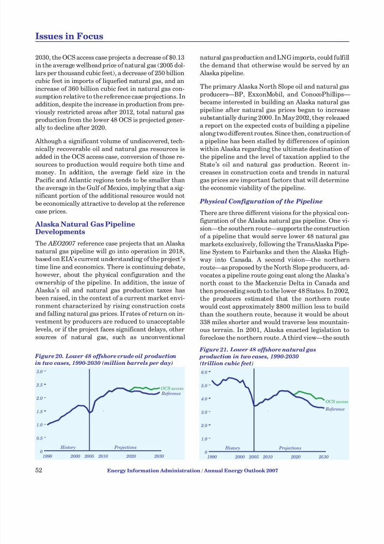
7/28/2019 2007 Annual Energy Outlook
http://slidepdf.com/reader/full/2007-annual-energy-outlook 61/243
2030, the OCS access case projects a decrease of $0.13in the average wellhead price of natural gas (2005 dol-lars per thousand cubic feet), a decrease of 250 billion
cubic feet in imports of liquefied natural gas, and anincrease of 360 billion cubic feet in natural gas con-
sumption relative to the reference case projections. Inaddition, despite the increase in production from pre-viously restricted areas after 2012, total natural gasproduction from the lower 48 OCS is projected gener-ally to decline after 2020.
Although a significant volume of undiscovered, tech-nically recoverable oil and natural gas resources isadded in the OCS access case, conversion of those re-sources to production would require both time andmoney. In addition, the average field size in thePacific and Atlantic regions tends to be smaller than
the average in the Gulf of Mexico, implying that a sig-nificant portion of the additional resource would not
be economically attractive to develop at the referencecase prices.
Alaska Natural Gas PipelineDevelopments
The AEO2007 reference case projects that an Alaska natural gas pipeline will go into operation in 2018,based on EIA’s current understanding of the project’s
time line and economics. There is continuing debate,however, about the physical configuration and the
ownership of the pipeline. In addition, the issue of Alaska’s oil and natural gas production taxes hasbeen raised, in the context of a current market envi-ronment characterized by rising construction costsand falling natural gas prices. If rates of return on in-vestment by producers are reduced to unacceptable
levels, or if the project faces significant delays, othersources of natural gas, such as unconventional
natural gas production and LNG imports, could fulfillthe demand that otherwise would be served by an
Alaska pipeline.
The primary Alaska North Slope oil and natural gas
producers—BP, ExxonMobil, and ConocoPhillips—became interested in building an Alaska natural gaspipeline after natural gas prices began to increasesubstantially during 2000. In May 2002, they releaseda report on the expected costs of building a pipeline
along two different routes. Since then, construction of a pipeline has been stalled by differences of opinionwithin Alaska regarding the ultimate destination of the pipeline and the level of taxation applied to theState’s oil and natural gas production. Recent in-creases in construction costs and trends in naturalgas prices are important factors that will determine
the economic viability of the pipeline.
Physical Configuration of the Pipeline
There are three different visions for the physical con-figuration of the Alaska natural gas pipeline. One vi-sion—the southern route—supports the constructionof a pipeline that would serve lower 48 natural gas
markets exclusively, following the TransAlaska Pipe-line System to Fairbanks and then the Alaska High-way into Canada. A second vision—the northernroute—as proposed by the North Slope producers, ad-vocates a pipeline route going east along the Alaska’s
north coast to the Mackenzie Delta in Canada andthen proceeding south to the lower 48 States. In 2002,the producers estimated that the northern route
would cost approximately $800 million less to buildthan the southern route, because it would be about338 miles shorter and would traverse less mountain-ous terrain. In 2001, Alaska enacted legislation toforeclose the northern route. A third view—the south
52 Energy Information Administration / Annual Energy Outlook 2007
Issues in Focus
1990 2000 2005 2010 2020 20300.0
0.5
1.0
1.5
2.0
2.5
3.0
Reference
History Projections
OCS access
Figure 20. Lower 48 offshore crude oil production
in two cases, 1990-2030 (million barrels per day)
1990 2000 2005 2010 2020 20300.0
1.0
2.0
3.0
4.0
5.0
6.0
Reference
History Projections
OCS access
Figure 21. Lower 48 offshore natural gas
production in two cases, 1990-2030
(trillion cubic feet)

7/28/2019 2007 Annual Energy Outlook
http://slidepdf.com/reader/full/2007-annual-energy-outlook 62/243
central design—supports the construction of a pipe-line that would transport natural gas to south central
Alaska, both to serve local consumers and to provide
LNG to overseas consumers.
The three pipeline proposals are based on fundamen-tally different priorities. The northern and southernroutes are premised on the notion that an Alaska nat-ural gas pipeline would be economically feasible onlyif it captured the greatest possible economies of scale
(the greatest pipeline throughput), thereby ensuring the highest possible wellhead price for North Slopenatural gas and the greatest State royalty collection.The south central design is premised largely on theidea that, because natural gas reserves in the Cook In-let region are declining, North Slope productionshould be transported to south central Alaska to en-
sure the future availability of natural gas to that re-gion’s consumers.
Production Taxes
The Alaska Stranded Natural Gas Development Actwas signed in 1998 to make a natural gas pipeline pro-
ject in Alaska commercially feasible. When the Act
was passed, lower 48 wellhead natural gas prices av-eraged $1.96 per thousand cubic feet. Since then, aslower 48 prices have increased, the political climate in
Alaska has changed from one in which financial in-centives were thought to be crucial to the construc-
tion of a pipeline to one in which some interestsbelieve that State taxes on oil and natural gas produc-tion are not high enough.
In May 2006, a draft stranded gas contract was madepublicly available. In the draft, the North Slope pro-ducers and the State agreed to a 20-percent produc-tion tax with a 20-percent tax credit for futureinvestments in Alaska’s oil and natural gas develop-ment. The terms and conditions were negotiated to
remain in effect for the next 30 years. After the re-lease of the draft contact, opponents argued that thecontract’s production tax rate was too low and the in-
vestment credits too large.
In August 2006, the Alaska legislature in a special ses-sion passed an oil and natural gas production tax,
which raised the oil production tax from the negoti-ated 20 percent up to 22.5 percent. The legislation,which was signed into law that same month, also re-duced the level of investment tax credits that NorthSlope producers could use to offset their productiontax liabilities.
At a minimum, the discrepancy between the provi-sions in the August 2006 law and the draft standardgas contract will necessitate renegotiation between
the producers and the State. The governor who nego-tiated the draft contract and signed the August 2006
law was defeated in his bid for reelection. The pipelinewas a major issue in the campaign, and the new gover-nor may not want to use the existing draft contract asthe starting point for negotiation.
Other Issues
Until the State of Alaska and the North Slope produc-ers come to some agreement on an Alaska natural gaspipeline, a number of other issues will remain unre-
solved. One issue is whether the State should be anequity investor and owner of the pipeline [105 ]. An-other involves the issuing of environmental permits
for the pipeline route, a process that has been conten-tious for other pipeline projects, sometimes resulting in significant delays.
A third issue is who will construct, own, and operatethe portion of an Alaska natural gas pipeline thatruns through Canada. TransCanada Pipelines main-tains that it has the legislated right to be the ownerand operator of the Canadian portion, as specified
in Canada’s Northern Pipeline Act of 1978 [106].Finally, the pipeline’s regulatory framework couldprove contentious. For the portion located within
the confines of the State, Alaska’s Regulatory Com-mission will have jurisdiction over rates and tariffs,including the terms and conditions associated withthird-party access to the pipeline. These other issueswill not be fully addressed until after all the issues be-tween the State and the North Slope producers have
been resolved, and it is not clear how contentious theissues will be or how quickly they can be settled.
Construction Costs and Natural Gas Prices
In May 2002, the three primary Alaska North Slopeproducers estimated the cost of construction for a
proposed southern route pipeline to the Chicago area and its associated facilities at approximately $19.4billion [107 ]. On the basis of that capital cost, theyestimated a pipeline transportation tariff of $2.39
per thousand cubic feet for natural gas moving fromthe North Slope to Chicago. From May 2002 to June2006, however, iron and steel prices increased by 72percent [108]. Although it has been estimated thatonly 25 percent of the total pipeline cost would be as-sociated with steel pipe, construction costs have been
Energy Information Administration / Annual Energy Outlook 2007 53
Issues in Focus

7/28/2019 2007 Annual Energy Outlook
http://slidepdf.com/reader/full/2007-annual-energy-outlook 63/243
increasing across the board, as equipment, labor, andcontractor costs have also risen.
A Federal law enacted in 2004 permits the Secretaryof Energy to issue Federal loan guarantees for the
construction of an Alaska natural gas pipeline. Theguarantees would be limited to 80 percent of the pipe-line’s total cost, up to a maximum of $18 billion. Be -cause the Federal loan guarantees would lower therisk associated with recovery of the project’s capitalcosts, pipeline sponsors would be able to secure debtfinancing at a lower interest rate than they could inthe absence of such guarantees, and the pipeline’s fi-nancial viability would be enhanced.
Recent increases in natural gas prices, which began in2000, have also improved the economic outlook foran Alaska natural gas pipeline. Lower 48 wellhead
prices, which averaged $2.19 per thousand cubic feetin 1999, rose to an average of $7.51 per thousand cu-bic feet in 2005. Although prices have declined since
then, the AEO2007 reference case price projectionsare at a level at which an Alaska natural gas pipelinewould remain economically viable if other issues sur-rounding the project could be resolved in a mannerthat met the needs of all parties. The parties wouldhave to agree on a division of the projected benefitsbefore the pipeline could be built.
Coal Transportation Issues
Most of the coal delivered to U.S. consumers is trans-ported by railroads, which accounted for 64 percent of total domestic coal shipments in 2004 [109]. Truckstransported approximately 12 percent of the coal con-sumed in the United States in 2004, mainly in shorthauls from mines in the East to nearby coal-fired elec-
tricity and industrial plants. A number of minemouthpower plants in the West also use trucks to haul coalfrom adjacent mining operations. Other significantmodes of coal transportation in 2004 included con-veyor belt and slurry pipeline (12 percent) and watertransport on inland waterways, the Great Lakes, andtidewater areas (9 percent) [110].
Rail is particularly important for long-haul ship-ments of coal, such as the transport of subbituminouscoal from mines in Wyoming to power plants in theeastern United States. In 2004, rail was the primarymode of transportation for 98 percent of the coal
shipped from Wyoming to customers in other States.
Rail Transportation Rates
When the railroad industry was deregulated in theearly 1980s, consumers benefited from a long period
of declining coal transportation rates. For coal ship-ments to electric utilities, rates in constant dollarsper ton fell by 42 percent from 1984 to 2001 [111].
More recently, railroads have been raising base trans-portation rates and implementing fuel surcharge pro-
grams. There are also concerns that railroads arefailing to meet their common carrier obligation withregard to reliability of service [112].
The national average rate for coal transportation in
2005 was approximately 6 percent higher (in constantdollars) than in 2004 [113]; and according to BNSF,average revenue per car in the first 6 months of 2006was 7 percent higher than in the same period of 2005as a result of contract rate escalations, fuel sur-charges, and increases in hauling distances [114]. Re-cent increases in rates have caused shippers to
question their fairness and to raise the possibilitythat the railroads may be exercising market power.
Since deregulation, four railroads have dominatedrail transportation of coal: CSX Transportation (CSX)and NS in the East and UP and BNSF in the West.
The concentration of coal freight business among a few carriers has led to claims of pricing power, in par-ticular from coal shippers that have no alternative to
relying on a single railroad. In 2004, when both UPand BNSF made their rates public by posting them ontheir web sites, some called it price collusion, in thatthe two companies could see each other’s rates and,
potentially, harmonize them. In February 2005, theU.S. Department of Justice initiated an investigationof their pricing activities. In October 2006, while notdrawing any conclusions, the Government Account-
ability Office recommended that the state of competi-tion in the freight railroad industry be analyzed [115 ].
The U.S. Department of Transportation’s Surface
Transportation Board (STB) has also been asked toreview the reasonableness of rates imposed on somecaptive customers. Typically, for a rate case to bebrought before the STB, there must be evidence sug-
gesting not only that the railroads charge more than180 percent of their variable cost to the captive ship-per but also that construction of a new rail line toserve the captive customer’s needs would be moreeconomical than the prices currently charged. In
cases decided from 2004 through June 2006, oneshowed an unreasonable rate, three were settled vol-untarily, and two were decided in favor of the rail-roads [116]. Because concerns have been raised aboutthe cost and time involved in preparing rate cases, theSTB instituted a series of rulemakings in 2006 to
54 Energy Information Administration / Annual Energy Outlook 2007
Issues in Focus

7/28/2019 2007 Annual Energy Outlook
http://slidepdf.com/reader/full/2007-annual-energy-outlook 64/243
improve the process by modifying its methods andprocedures for large rail rate disputes and revising itssimplified guidelines for smaller rate disputes.
A number of factors, including railroad profitability,
the need for more investment, and increased fuel ex-penses in recent years, may be contributing to the re-cent increase in coal transportation rates. One motivefor price increases by the railroads is to improve theirrate of return on investment. The STB identifies a
railroad as “revenue adequate” if its return on invest-ment exceeds the industry’s average cost of capital, asestimated by the STB. By this standard, only NS wasconsidered revenue adequate in 2004 and 2005,whereas none of the railroads was considered revenueadequate in 2003 [117 ].
The railroads have argued that, after deregulation,savings resulting from consolidation of redundant in-frastructure were passed on to their customers, butthat such savings are no longer attainable. Instead,they typically state that higher prices are needed toadd infrastructure in order to keep pace with demand.Most recently, each of the railroads has instituted a fuel surcharge program in response to rising fuelprices. The surcharge programs have been cited by
many of the railroads as a success, and they have con-tributed to record-breaking profits. UP, for instance,reported profits for the fourth quarter of 2005 thatwere triple those of the fourth quarter of 2004 [118].
Some rail customers in the coal industry have in turnclaimed that the railroads are “double dipping,” re-covering more through the surcharges than theyspend on fuel.
The railroads have maintained that their fuel sur-charge programs are transparent, but most custom-ers appear to disagree. Each of the railroads hasimplemented its program differently, choosing differ-ent fuel price targets and thresholds that trigger thesurcharge. For instance, BNSF and UP use EIA’s
on-highway diesel price as the basis for determining
whether a fuel surcharge will be implemented,whereas NS and CSX use the WTI crude oil price. Asof July 1, 2006, NS was applying a surcharge whenthe monthly WTI average price exceeded $64 per bar-rel [119]. CSX begins its price adjustments when the
WTI price reaches $23.01 per barrel [120].
The STB has stated that the surcharge programs,while not unreasonable, were implemented in an un-reasonable manner that lacked transparency. It si-multaneously recommended the use of a program
that would be linked more tightly to actual fuel usageand would require all carriers to use the same fuel in-dex [121]. The response from the railroads has been
mixed, with BNSF stating that the STB lacks author-ity to make a ruling unless a formal shipper’s com-
plaint is brought forward [122] and CSX expressing a willingness to comply “under future guidance fromthe STB” [123].
Wyoming Powder River Basin
One of the most important U.S. coal-producing areas
is Wyoming’s Powder River Basin. Almost all the coalproduced there is carried out by rail, and disruptionsin the rail transportation network can have signifi-cant effects on the flow of coal from the region. Keyfactors that can lead to disruptions include the needto perform major maintenance on important seg-
ments of a rail corridor and the development of bottle-necks due to unforeseen growth in the demand for rail
transportation services. The problems that arose inthe Powder River Basin in 2005 and 2006 illustratethe potential impact of these factors.
In May 2005, adverse weather conditions and accu-mulated coal dust in the roadbed of the Joint Linerailroad combined to create track instability that con-
tributed to two train derailments. The Joint LineRailroad, a 103-mile stretch of dedicated coal railway,is jointly owned and operated by BNSF and UP. It
serves 8 of the 14 active coal mines in Wyoming’sPowder River Basin and is one of the most heavilyused sections of rail line in the world.
During 2005 and 2006, coal shippers expressed theirconcerns about operating conditions on the Joint Linein testimony before both houses of Congress and theFERC. Some power plant operators indicated that in-adequate shipments of coal from the Powder River
Basin had forced them to draw down their on-sitestockpiles of coal to unprecedented levels in early tomid-2006. Others said they were forced to dispatchmore expensive generating capacity, purchase elec-tricity from other generators to meet customer de-mand, or buy high-priced coal on the spot market orfrom offshore suppliers. In testimony before the U.S.Senate in May 2006, EIA indicated that monthly data reported by electric power plants did show a drop in
inventories of subbituminous coal (most of which co-mes from Wyoming) from mid-2005 through early2006, consistent with press reports that generatorsrelying on subbituminous coal were taking steps toconserve coal supplies [124].
Energy Information Administration / Annual Energy Outlook 2007 55
Issues in Focus

7/28/2019 2007 Annual Energy Outlook
http://slidepdf.com/reader/full/2007-annual-energy-outlook 65/243
A study recently produced for the U.S. Bureau of Land Management found that capacity utilization of the Joint Line in 2003 exceeded 88 percent, as com-
pared with 22 percent for the BNSF rail line thatserved five active Wyoming mines north of the Joint
Line in 2003 (Wyodak, Dry Fork, Rawhide, EagleButte, and Buckskin). The combined output of thosemines has increased significantly, from 55 milliontons in 2003 to 65 million tons in 2005, and is likely tosurpass 70 million tons in 2006. As a result, utiliza-tion of the BNSF line is now slightly higher than itwas in 2003. The mines served by the Joint Line pro-
duced and shipped 325 million tons of coal in 2005, ac-counting for 29 percent of the year’s total U.S. coalproduction. Joint Line shipments for the year were 3million tons higher than in 2004 but still 20 milliontons less than had been planned [125 ].
BNSF and UP have completed maintenance work re-
lated to the 2005 train derailments and have em-barked on major upgrades to increase haulagecapacity on the Joint Line; however, demand in 2006was expected to exceed the capability of the railroadsand mines to supply coal from the area to the market.In mid-2006, a representative from BNSF indicatedthat the potential demand for Powder River Basincoal for the year probably would exceed supply by 20
to 25 million tons [126]. Through August 2006, coalshipments on the Joint Line were 9 percent higherthan in the same period of 2005, corresponding to anannualized increase of approximately 25 million tons.
Beyond 2006, investments in new track and railequipment for the Joint Line indicate an improved
outlook for shipping capacity. Recently announcedplans for investments in 2005 through 2007, totaling about $200 million, will add nearly 80 miles of thirdand fourth mainline track to the Joint Line, increas-ing annual shipping capacity to almost 420 milliontons [127 ]. In a recent study for BNSF and UP, theconsulting firm CANAC identified investments thatcould further increase the Joint Line’s capacity to ap-
proximately 500 million tons by 2012 [128]. The po-tential increase in shipments was arrived at throughdiscussions with individual mine operators along the
Joint Line. According to the study, an additional 80million tons of shipping capacity after 2007 would re-quire the construction of 12 new loading spots atmines and 45 additional miles of mainline track. Alsokey to meeting the target of 500 million tons is the ex-pectation that railroads will be able to move graduallyto longer trains over the next few years, from current
lengths of 125 to 130 cars to approximately 150 cars[129].
The authors of the CANAC report indicated that thetiming of investments will depend on the market for
Powder River Basin coal in coming years and coulddeviate from the schedule outlined. Although produc-tion from mines on the Joint Line were not explicitlymodeled by EIA, the projected growth of coal produc-tion from Wyoming’s Powder River Basin in the
AEO2007 reference case is not inconsistent with theexpansion potential identified in the CANAC report.In all the cases modeled for AEO2007 , the projectedincrease in annual coal production from active minesin Wyoming’s Powder River Basin is less than 175million tons (the sum of Joint Line expansion projectsidentified in the report) until after 2019.
Another potential investment under consideration isan expansion of the Dakota Minnesota & EasternRailroad (DM&E) westward to the Powder River Ba-sin. The project would include 280 miles of new con-struction and provide an alternative rail option for
Wyoming coal. It would provide access to the minescurrently active south of Gillette, Wyoming, andwould be independent of the existing Joint Line [130].
The extension would provide enough rail capacity forthe transport of 100 million tons of coal annually ac-cording to DM&E, which is seeking a loan from theFederal Railroad Administration to support it.
Coal Production and Consumption Projections
in AEO2007
In the AEO2007 reference case, coal remains the pri-mary fuel for electricity generation through 2030.Coal production is projected to increase significantly,particularly in the Powder River Basin. From 2005 to2030, production in the Wyoming Powder River Basinis projected to grow by 289 million tons, but the pro-
jected annual increases do not exceed 30 million tons.The resulting increase in coal transport requirementsis not beyond the level of expansion projects currently
being discussed.
The Rocky Mountain, Central West, and East NorthCentral regions are projected to show the largest in-
creases in coal demand, by about 100 million tonseach, from 2005 to 2030. The majority of the coal de-livered to the Rocky Mountain region is projected tocontinue to come from Colorado and Utah. In addi-tion, most of the growth in the region is projected tocome from new plants that are likely to be built as
56 Energy Information Administration / Annual Energy Outlook 2007
Issues in Focus

7/28/2019 2007 Annual Energy Outlook
http://slidepdf.com/reader/full/2007-annual-energy-outlook 66/243
close as possible to supply sources, potentially reduc-ing the need for extensive new development of rail in-frastructure. At a minimum, new plants will be
located only after careful consideration of transporta -tion options, to reduce the potential for rail bottle-
necks. For the Central West region, 42 percent of theincrease in coal demand is projected to be supplied by
Wyoming Powder River Basin coal; however, the larg-est supply increase (meeting 55 percent of the re-gion’s total increase in demand) is projected to comefrom the Dakota lignite supply region, to providefeedstocks for new CTL plants that are likely to be sit-
uated as close to their supply sources as possible.
In the East North Central region, most of the coalsupply to meet the projected growth in consumption(120 million tons from 2005 to 2030) is expected tocome from the Wyoming Powder River Basin. The in-crease in the region’s demand for coal could lead to
congestion on heavily traveled rail lines, such as thosesurrounding the Chicago area, where coal and otherbulk commodities already make heavy use of the sys-tem. The strongest growth in the region’s coal con-sumption is projected to occur between 2020 and2025, when deliveries from Wyoming’s Powder RiverBasin are projected to grow by 43 million tons, withthe largest single-year increase being 12 million tons.
Biofuels in the U.S. TransportationSector
Sustained high world oil prices and the passage of theEPACT2005 have encouraged the use of agriculture-based ethanol and biodiesel in the transportation sec-tor; however, both the continued growth of thebiofuels industry and the long-term market potentialfor biofuels depend on the resolution of critical issues
that influence the supply of and demand for biofuels.For each of the major biofuels—corn-based ethanol,cellulosic ethanol, and biodiesel—resolution of tech-nical, economic, and regulatory issues remains criti-cal to further development of biofuels in the UnitedStates.
In the transportation sector, ethanol is the mostwidely used liquid biofuel in the world. In the UnitedStates, nearly all ethanol is blended into gasoline atup to 10 percent by volume to produce a fuel calledE10 or “gasohol.” In 2005, total U.S. ethanol produc-tion was 3.9 billion gallons, or 2.9 percent of the totalgasoline pool. Preliminary data for 2006 indicate thatethanol use rose to 5.4 billion gallons. Biodiesel pro-duction was 91 million gallons, or 0.21 percent of
the U.S. distillate fuel oil market, including diesel, in
2005 (Table 11). All cars and light trucks built for theU.S. market since the late 1970s can run on the etha-nol blend E10. Automakers also produce a limited
number of FFVs for the U.S. market that can run onany blend of gasoline and ethanol up to 85 percent
ethanol by volume (E85). Because auto manufactur-ers have been able to use FFV sales to offset CAFE re-quirements, more than 5 million FFVs were producedfor the U.S. market from 1992 through 2005. E10 fuelis widely available in many States. E85 has limitedavailability, at stations clustered mostly in the mid-western States.
In the AEO2007 reference case, ethanol use increasesrapidly from current levels. Ethanol blended into gas-oline is projected to account for 4.3 percent of the to-tal gasoline pool by volume in 2007, 7.5 percent in
2012, and 7.6 percent in 2030. As a result, gasoline de-mand increases more rapidly in terms of fuel volume
(but not in terms of energy content) than it would inthe absence of ethanol blending. Overall, gasolineconsumption is projected to increase by 32 percent onan energy basis, and by 34 percent on a volume basis,from 2007 to 2030.
Ethanol can be produced from any feedstock that con-
tains plentiful natural sugars or starch that can bereadily converted to sugar. Popular feedstocks in-clude sugar cane (Brazil), sugar beets (Europe), andmaize/corn (United States). Ethanol is produced by
fermenting sugars. Corn grain is processed to removethe sugar in wet and dry mills (by crushing, soaking,and/or chemical treatment), the sugar is fermented,and the resulting mix is distilled and purified to ob-
tain anhydrous ethanol. Major byproducts from theethanol production process include dried distillers’
Energy Information Administration / Annual Energy Outlook 2007 57
Issues in Focus
Gasoline Ethanol Percent of
gasoline pool
2000 128,662 1,630 1.27
2001 129,312 1,770 1.37 2002 132,782 2,130 1.60
2003 134,089 2,800 2.09
2004 137,022 3,400 2.48
2005 136,949 3,904 2.85
Diesel Biodiesel Percent of
diesel fuel pool
2000 37,238 — —
2001 38,155 9 0.02
2002 38,881 11 0.03
2003 40,856 18 0.04
2004 42,773 28 0.07
2005 43,180 91 0.21
Table 11. U.S. motor fuels consumption, 2000-2005
(million gallons per year)

7/28/2019 2007 Annual Energy Outlook
http://slidepdf.com/reader/full/2007-annual-energy-outlook 67/243
grains and solubles (DDGS), which can be used as ani-mal feed. On a smaller scale, corn gluten meal, glutenfeed, corn oil, CO2, and sweeteners are also byprod-
ucts of the ethanol production process used in theUnited States.
With additional processing, plants and other biomass
residues (including urban wood waste, forestry resi-due, paper and pulp liquors, and agricultural residue)can be processed into fermentable sugars. Such po-tentially low-cost resources could be exploited to yieldsignificant quantities of fuel-quality ethanol, generi-cally termed “cellulosic ethanol.” Cellulose andhemicellulose in biomass can be broken down into fer-mentable sugars by either acid or enzymatic hydroly-
sis. The main byproduct, lignin, can be burned forsteam or power generation. Alternatively, biomass
can be converted to synthesis gas (hydrogen and car-bon monoxide) and made into ethanol by the Fischer-Tropsch process or by using specialized microbes.
Capital costs for a first-of-a-kind cellulosic ethanolplant with a capacity of 50 million gallon per year areestimated by one leading producer to be $375 million(2005 dollars) [131], as compared with $67 million fora corn-based plant of similar size, and investment riskis high for a large-scale cellulosic ethanol productionfacility. Other studies have provided lower cost esti-
mates. A detailed study by the National RenewableEnergy Laboratory in 2002 estimated total capital
costs for a cellulosic ethanol plant with a capacity of 69.3 million gallons per year at $200 million [132].The study concluded that the costs (including capitaland operating costs) remained too high in 2002 for a company to begin construction of a first-of-its-kindplant without significant short-term advantages,such as low costs for feedstocks, waste treatment, or
energy.
If future oil prices follow a path close to that in the
AEO2007 reference case, significant reductions in thecapital cost and operating costs of a cellulosic ethanol
plant will be needed for cellulosic ethanol to be eco-nomically competitive with petroleum-based fuels.The extent to which costs can be reduced through a combination of advances in the production process forcellulosic ethanol and learning as plants are con-structed in series will be important to the future com-petitiveness of cellulosic ethanol. World oil price
developments also will play a central role.
Currently, no large-scale cellulosic ethanol produc-
tion facilities are operating or under construction.
EPACT2005 provides financial incentives that in the AEO2007 reference case are projected to bring thefirst cellulosic ethanol production facilities on line
between 2010 and 2015, with a total capacity of 250million gallons per year. Cellulosic ethanol currently
is not cost-competitive with gasoline or corn-basedethanol, but considerable R&D by the National Re-newable Energy Laboratory and its partners hassignificantly reduced the estimated cost of enzymeproduction. Although technological breakthroughsare inherently unpredictable, further significant suc-cesses in R&D could make cellulosic ethanol a viable
economic option for expanded ethanol production inthe future.
Biodiesel is a renewable-based diesel substitute usedin Europe with early commercial market develop-
ment in the United States. Biodiesel is composed of mono-alkyl esters of long-chain fatty acids derived
from vegetable oils or animal fats [133]. Itis similar todistillate fuel oil (diesel fuel) and can be used in thesame applications, but it has different chemical, han-dling, and combustion characteristics. Biodiesel canbe blended with petroleum diesel in any fraction andused in compression-ignition engines, so long as thefuel system that uses it is constructed of materialsthat are compatible with the blend. The high lubricity
of biodiesel helps to offset the impact of adopting low-sulfur diesel.
Common blends of biodiesel are 2 percent, 5 percent,and 20 percent (B2, B5, and B20). Individual enginemanufacturers determine which blends are war-ranted for use in their engines, but generally B5
blends are permissible and some manufacturers sup-port B20 blends. Blends of biodiesel are distributed atstations throughout the United States. Some Stateshave mandated levels of biodiesel use when in-Stateproduction reaches prescribed levels.
Predominant feedstocks for biodiesel production are
soybean oil in the United States, rapeseed and sun-
flower oil in Europe, and palm oil in Malaysia.Biodiesel also can be produced from a variety of otherfeedstocks, including vegetable oils, tallow and ani-mal fats, and restaurant waste and trap grease. Toproduce biodiesel, raw vegetable oil is chemicallytreated in a process called transesterification. Theproperties of the biodiesel (cloud point, pour point,and cetane number) depend on the type of feedstock
used. Crude glycerin, a major byproduct of the reac-tion, usually is sold to the pharmaceutical, food, andcosmetic industries.
58 Energy Information Administration / Annual Energy Outlook 2007
Issues in Focus

7/28/2019 2007 Annual Energy Outlook
http://slidepdf.com/reader/full/2007-annual-energy-outlook 68/243
Energy Content and Fuel Volume
On a volumetric basis, ethanol and biodiesel havelower energy contents than do gasoline and distillatefuel oil, respectively. Table 12 compares the energy
contents of various fuels on the basis of Btu per gallonand gallons of gasoline equivalent. The table showsboth the low heating value (the amount of heat re-leased by the fuel, ignoring the latent heat of vapor-ization of water) and the high heating value (theamount of heat released by the fuel, including the la-
tent heat of vaporization of water). The lower energycontent of ethanol and biodiesel generally results in a commensurate reduction in miles per gallon whenthey are used in engines designed to run on gasolineor diesel. Small-percentage blends of ethanol andbiodiesel (E10, B2, and B5) result in smaller losses of fuel economy than do biofuel-rich blends (E85 andB20).
Today, most fuel ethanol is used in gasoline blends,where it accounts for as much as 10 percent of eachgallon of fuel—a level that all cars can accommodate.In higher blends, ethanol can make up as much as 85percent of each gallon of fuel by volume. In the future,increased use of ethanol as a transportation fuel will
raise the issue of fuel volume versus energy content.Ethanol contains less energy per gallon than doesconventional gasoline. A gallon of ethanol has onlytwo-thirds the energy of a gallon of conventional gaso-
line, and the number of miles traveled by a given vehi-cle per gallon of fuel is directly proportional to theenergy contained in the fuel.
E10 (10 percent ethanol) has 3.3 percent less energycontent per gallon than conventional gasoline. E85(which currently averages 74 percent ethanol by vol-ume) has 24.7 percent less energy per gallon thanconventional gasoline. AEO2007 assumes that enginethermal efficiency remains the same whether the ve-hicle burns conventional gasoline, E10, or E85. Thismeans that 1.03 gallons of E10 or 1.33 gallons of E85
are needed for a vehicle to cover the same distancethat it would with a gallon of conventional gasoline.
Although the difference is not expected to have a
significant effect on purchases of E10, AEO2007 as-sumes that motorists whose vehicles are able to runon E85 or conventional gasoline will compare the two
fuels on the basis of price per unit of energy.
The issue of gasoline energy content first arose inthe early 1990s with the introduction of oxygenatedgasoline made by blending conventional gasoline with15 percent MTBE or 7.7 percent ethanol by volume.
When oxygenated gasoline was introduced, MTBE
was the blending agent of choice. Since then, ethanolhas steadily replaced MTBE in oxygenated and RFGblends. The fuel economy impact of switching fromMTBE-blended gasoline to an ethanol blend issmaller than the impact of switching from conven-tional gasoline. For example, changing from 15 per-cent MTBE to 7.7 percent ethanol in blended gasoline
results in a reduction in energy content of only 1.2percent per gallon of fuel, and changing from 15 per-
cent MTBE to 10 percent ethanol results in a reduc-tion of 1.9 percent.
Current State of the Biofuels Industry
The nascent U.S. biofuel industry has recently begun
a period of rapid growth. Over the past 6 years,biofuel production has been growing both in absoluteterms and as a percentage of the gasoline and dieselfuel pools (see Table 11). High world oil prices, firmgovernment support, growing environmental and en-
ergy security concerns, and the availability of low-cost corn and soybean feedstocks provide favor-able market conditions for biofuels. Ethanol, in par-
ticular, has been buoyed by the need to replace theoctane and clean-burning properties of MTBE, whichhas been removed from gasoline because of concernsabout groundwater contamination. About 3.9 billiongallons of ethanol and 91 million gallons of biodieselwere produced in the United States in 2005. Accord-ing to estimates based on the number of plants underconstruction, ethanol production capacity could riseto about 7.5 billion gallons and biodiesel capacity to
about 1.1 billion gallons by 2008, possibly resulting inexcess capacity in the near term (Figure 22).
Energy Information Administration / Annual Energy Outlook 2007 59
Issues in Focus
Fuel Btu per gallon
(low heating value) Btu per gallon
(high heating value)Gallons of gasoline equivalent
(high heating value)
Conventional gasoline 115,500 125,071 1.00
Fuel ethanol (E100) 76,000 84,262 0.67
E85 (74% blend on average) — 94,872 0.76
Distillate fuel oil (diesel) 128,500 138,690 1.11
Biodiesel (B100) 118,296 128,520 0.95
Table 12. Energy content of biofuels
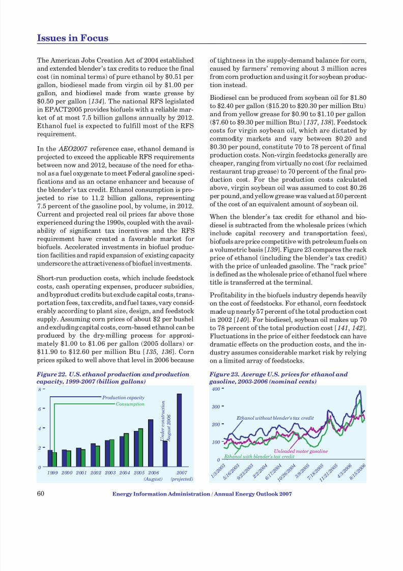
7/28/2019 2007 Annual Energy Outlook
http://slidepdf.com/reader/full/2007-annual-energy-outlook 69/243
The American Jobs Creation Act of 2004 establishedand extended blender’s tax credits to reduce the finalcost (in nominal terms) of pure ethanol by $0.51 per
gallon, biodiesel made from virgin oil by $1.00 pergallon, and biodiesel made from waste grease by
$0.50 per gallon [134]. The national RFS legislatedin EPACT2005 provides biofuels with a reliable mar-ket of at most 7.5 billion gallons annually by 2012.Ethanol fuel is expected to fulfill most of the RFSrequirement.
In the AEO2007 reference case, ethanol demand isprojected to exceed the applicable RFS requirementsbetween now and 2012, because of the need for etha-nol as a fuel oxygenate to meet Federal gasoline speci-
fications and as an octane enhancer and because of the blender’s tax credit. Ethanol consumption is pro-
jected to rise to 11.2 billion gallons, representing 7.5 percent of the gasoline pool, by volume, in 2012.Current and projected real oil prices far above thoseexperienced during the 1990s, coupled with the avail-ability of significant tax incentives and the RFSrequirement have created a favorable market forbiofuels. Accelerated investments in biofuel produc-
tion facilities and rapid expansion of existing capacityunderscore the attractiveness of biofuel investments.
Short-run production costs, which include feedstock
costs, cash operating expenses, producer subsidies,and byproduct credits but exclude capital costs, trans-
portation fees, tax credits, and fuel taxes, vary consid-erably according to plant size, design, and feedstocksupply. Assuming corn prices of about $2 per busheland excluding capital costs, corn-based ethanol can beproduced by the dry-milling process for approxi-mately $1.00 to $1.06 per gallon (2005 dollars) or$11.90 to $12.60 per million Btu [135 , 136]. Corn
prices spiked to well above that level in 2006 because
of tightness in the supply-demand balance for corn,caused by farmers’ removing about 3 million acresfrom corn production and using it for soybean produc-
tion instead.
Biodiesel can be produced from soybean oil for $1.80to $2.40 per gallon ($15.20 to $20.30 per million Btu)and from yellow grease for $0.90 to $1.10 per gallon
($7.60 to $9.30 per million Btu) [137 , 138]. Feedstockcosts for virgin soybean oil, which are dictated bycommodity markets and vary between $0.20 and$0.30 per pound, constitute 70 to 78 percent of finalproduction costs. Non-virgin feedstocks generally arecheaper, ranging from virtually no cost (for reclaimedrestaurant trap grease) to 70 percent of the final pro-duction cost. For the production costs calculatedabove, virgin soybean oil was assumed to cost $0.26
per pound, and yellow grease was valued at 50 percentof the cost of an equivalent amount of soybean oil.
When the blender’s tax credit for ethanol and bio-
diesel is subtracted from the wholesale prices (whichinclude capital recovery and transportation fees),biofuels are price competitive with petroleum fuels ona volumetric basis [139]. Figure 23 compares the rackprice of ethanol (including the blender’s tax credit)with the price of unleaded gasoline. The “rack price”is defined as the wholesale price of ethanol fuel wheretitle is transferred at the terminal.
Profitability in the biofuels industry depends heavilyon the cost of feedstocks. For ethanol, corn feedstockmade up nearly 57 percent of the total production costin 2002 [140]. For biodiesel, soybean oil makes up 70
to 78 percent of the total production cost [141, 142].Fluctuations in the price of either feedstock can havedramatic effects on the production costs, and the in-dustry assumes considerable market risk by relying on a limited array of feedstocks.
60 Energy Information Administration / Annual Energy Outlook 2007
Issues in Focus
1 / 3 / 2 0
0 3
5 / 1 6
/ 2 0 0
3
9 / 2 3
/ 2 0 0
3
2 / 2 / 2 0
0 4
6 / 1 7
/ 2 0 0
4
1 0 / 2 6 / 2 0
0 4
3 / 9 / 2 0
0 5
7 / 1 8
/ 2 0 0
5
1 1 / 2 1 / 2 0
0 5
4 / 3 / 2 0
0 6
8 / 1 5
/ 2 0 0
6
0
100
200
300
400
Ethanol without blender's tax credit
Unleaded motor gasoline Ethanol with blender's tax credit
Figure 23. Average U.S. prices for ethanol and
gasoline, 2003-2006 (nominal cents)
1999 2000 2001 2002 2003 2004 2005 2006
(August)
2007
(projected)
0
2
4
6
8
Production capacity
Consumption
U n
d e r
c o n s t r u c t i o n
A u g u s t
2 0 0 6
Figure 22. U.S. ethanol production and production
capacity, 1999-2007 (billion gallons)

7/28/2019 2007 Annual Energy Outlook
http://slidepdf.com/reader/full/2007-annual-energy-outlook 70/243
The U.S. ethanol industry relies almost exclusively oncorn, consuming 20 percent of the available corn sup-ply in 2006[143]. At current production levels, corn—
which is produced domestically in large volumes—isthe most attractive feedstock for ethanol. As ethanol
production increases, competition for corn suppliesamong the fuel, food, and export markets, along witha decline in the marginal value of ethanol co-products,is expected to make production more expensive [144].
Assuming the development of cost-effective produc-tion facilities, cellulosic biomass feedstocks likeswitchgrass, agricultural residues, and hybrid poplartrees could supply a growing ethanol industry withlarge quantities of less expensive raw materials. Todifferentiate the current use of corn with the futureuse of cellulosic biomass and the differences in pro-
duction technology, corn is generally characterized asa “first generation” energy crop, whereas switchgrass
and other cellulosic materials are “second genera-tion” energy crops.
The U.S. biodiesel industry relies almost exclusivelyon soybean oil as a feedstock. Soybean oil has histori-cally been a surplus product of the oilmeal crushing industry, available in large quantities at relatively
low prices. At production levels nearing 300 to 600million gallons of biodiesel per year (less than 2 per-cent of the diesel fuel pool), the marginal cost of using soybean oil as a feedstock rises to the point where
other oilseeds—canola, rapeseed, sunflower, and cot-tonseed—become viable feedstocks [145 ]. There areno significant differences in processing for the nu-merous biodiesel feedstocks, and they cannot easily
be grouped into first- and second-generation catego-ries. The major differences among biodiesel feed-stocks are regional availability, co-product value, andthe composition of fatty acids in the refined vegetableoil.
Resource Utilization and Land Availability
Currently, corn and soybean feedstocks for biofuels
are grown almost exclusively on prime agriculturalland in the Midwest. Increases in the supply of biofuelfeedstocks could come from a combination of threestrategies: increasing the amount of land used ascropland, boosting the yields of existing energy crops,and replacing or supplementing corn with cellulosic
biomass and soybeans with oilseeds more appropriatefor biodiesel production. All three strategies may berequired to overcome the constraints of currentlyavailable feedstocks and sustain biofuel production
levels that could displace at least 10 percent of gaso-line consumption.
According to the most recent Agricultural Census(2002), the amount of cropland available in the lower
48 United States is 434 million acres [146], or 23 per-cent of the total land area [147 ]. The total amount of
cropland—defined as the sum of land used for crops,idle land, and pasture—has been declining for thepast 50 years and, increasingly, is becoming concen-trated in the Midwest. The trend is expected to con-tinue as population pressure leads to permanentconversion of some agricultural lands to other uses. Itis unlikely that additional cropland will be added inthe United States to accommodate increases in thedemand for biofuels. Instead, the cultivation of
biofuels will compete with other agricultural uses,
such as pastureland and idle land, much of which is inthe Conservation Reserve Program (CRP) [148].
The potential use of CRP acreage to grow corn andsoybeans is constrained by productivity, environmen-tal, and contractual limitations. Nevertheless, theremay be significant opportunities in the future to usesome CRP acres to grow such “low-impact” energycrops as native grasses (switchgrass) and short-rotation trees (willows or poplars) to generate cellu-losic biomass. Pilot programs are underway in Minne-
sota, Iowa, New York, and Pennsylvania to determinewhether CRP acres can be used to grow energy crops
while preserving the environmental mandate of theCRP.
Land Use and Productivity
With a limited supply of cropland available for biofuelfeedstocks, increasing yield (bushels per acre) on anannual basis could significantly boost available sup-plies of corn and soybeans without requiring addi-
tional land. With more than 81 million acres devotedto corn and nearly 72 million acres devoted to soy-beans (2005 U.S. planted acres), even small increasesin annual yield could boost supplies significantly[149].
There have been large annual increases in yields of both corn and soybeans over the past 30 years. Corn
yields increased from 86.4 bushels per acre in 1975 to151.2 bushels per acre in 2006, and soybean yields in-creased from 28.9 bushels per acre to 43 bushels peracre over the same period [150]. If corn yields con-tinue to increase at the same rate (approximately 1.8
bushels per acre per year), production could increase
Energy Information Administration / Annual Energy Outlook 2007 61
Issues in Focus

7/28/2019 2007 Annual Energy Outlook
http://slidepdf.com/reader/full/2007-annual-energy-outlook 71/243
by more than 3.1 billion bushels (29 percent) by 2030without requiring any additional acreage. Similarly,soybean production could increase by nearly 1.0 bil-
lion bushels per year by 2030 with no additional acre-age requirement if yields continue to grow at the rate
of 0.5 bushels per acre per year [151]. Improvementsin biofuel collection and refining and bioengineering of corn and soybeans also could contribute to im-proved biofuel yields. Research on methods to in-crease the starch content of corn and the oil content of soybeans is also ongoing.
Crop Competition
A key uncertainty is the availability of sufficient landresources for large-scale expansion of the cultivationof biofuel crops, given the intense competition withconventional agricultural products for arable land.
Competition will favor those crops most profitable forfarmers, accounting for such factors as growing re-gion, farming practice, and soil type. Currently, cornand soybeans are competitive energy crops, becausethey provide high value to farmers at prices lowenough to allow the biofuel industry to produce a product competitive with petroleum fuels.
Cellulosic biomass from switchgrass, hybrid willowand poplar trees, agricultural residues, and othersources has significant supply potential, possibly upto 4 times the potential of corn [152]. Switchgrass and
poplars could be grown on CRP lands, where corncannot be grown economically, but they would not becompetitive with corn until corn prices rose or the
capital and non-feedstock production costs of cellu-losic ethanol were significantly reduced. To expandbeyond a production level of 15 to 20 billion gallons
per year without seriously affecting food cropproduction and prices, the industry must make a
transition to crops with higher yields per acre andgrow crops in an environmentally permissible man-ner on CRP lands, while continuing to provide profitsfor producers.
Role of Co-products in Biofuel Economics
The value of co-products will play a significant role indetermining which crops are most profitable for farm-ers to grow and biofuel producers to use. High pricesfor raw crop material are desirable for farmers butundesirable for biofuel producers. High prices forco-products, on the other hand, increase revenues for
agricultural processors, sustain high prices for rawcrop materials, and offset feedstock costs for biodieselproducers. Corn and soybeans not only provide starchand oil for biofuel production but also generate signif-icant quantities of co-products, such as DDGS, glutenfeed, gluten meal, corn oil, and soybean oil meal withhigh protein content (Table 13). As a result, corngrain and soybean oil can be offered at prices lowerthan those of other feedstocks, and currently they are
the most competitive biofuel crops.
Co-products of the 3.9 billion gallons of ethanol pro-
duced in 2005 were significant, including 10 millionshort tons of DDGS, 473,000 short tons of corn glutenmeal, 2.6 million short tons of corn gluten feed, and
62 Energy Information Administration / Annual Energy Outlook 2007
Issues in Focus
Biofuel feedstock Co-products
Volume produced(pounds per
100 pounds of feedstock) Approximate value(dollars per pound)
Ethanol
Corn, wet mill Corn gluten feed 24.0 0.033
Corn gluten meal 4.5 0.135
Corn oil 2.9 0.260
Corn, dry mill Dried distillers’ grains and solubles 30.5 0.045
Sugar Sugar stalks, bagasse 27.0 —
Cellulosic ethanol
Switchgrass
Lignin27.0 — Hybrid poplar
Forest residue
Agricultural residue
Biodiesel
Soybeans Meal (44-48% protein) 80-82 0.097
Canola Meal (28-36% protein) 60-62 0.079
Sunflower Meal (28% protein) 60-63 0.035
Mustard Meal (28-36% protein) 60-62 —
Cotton Meal (41% protein) 84-86 0.088
Crude glycerin 10 0.050
Table 13. U.S. production and values of biofuel co-products

7/28/2019 2007 Annual Energy Outlook
http://slidepdf.com/reader/full/2007-annual-energy-outlook 72/243
283,000 short tons of corn oil [153]. As biofuel produc-tion continues to expand to the level of 7.5 billion gal-lons per year mandated in EPACT2005, production of
DDGS, used primarily as animal feed, will grow tomore than 12 million short tons annually and may de-
press prices in the feed market.
Biodiesel production in 2005 was considerably lessthan ethanol production, at 90.8 million gallons. Be-cause U.S. biodiesel production currently uses sur-
plus soybean oil (generated as a co-product in thesoybean meal industry), it has little effect on othermarkets for soybeans; however, annual production of 300 to 600 million gallons of biodiesel would begin tocompete with food and feed markets for soybeans[154]. For every 100 pounds of biodiesel production,about 10 pounds of crude glycerin is generated as a
co-product [155 ]. The glycerin generated by a 300 to600 million gallon per year biodiesel industry could
displace nearly one-half of the 692 million pounds of glycerin produced domestically in North America [156] and result in substantial oversupply.
Market Effects of Biofuel Growth
The feedstocks used to produce biofuels currentlymake up only 15 percent of available crop matter andare located at the end of a long agricultural supplychain. The markets for biofuels, biofuel co-products,and crop commodities are linked and susceptible to
changes in the prices and availability of crops. Surg-ing demand for biofuel feedstocks is likely to exert up-ward price pressure on corn and soybean commodities
and influence export, food, and industrial feedstockmarkets, particularly in the short term.
Co-product production also increases with biofuelproduction. At higher levels of biofuel production inthe future, co-products may be oversupplied, result-ing in depressed prices for the co-products and lower
revenues from their sale to offset fuel productioncosts. Finding new, high-value uses for co-productscould ensure that market prices for co-products re-
main stable. To the extent that other energy crops,such as switchgrass and inedible oilseeds, could begrown on less productive land (like the CRP), upwardpressure on the prices of corn, soybeans, and otherhigh-value food crops could also be mitigated.
Some studies have suggested that up to 16 billion gal-lons of ethanol (slightly more than 10 percent of thetotal gasoline pool by volume) can be produced fromcorn in 2015 without adversely affecting the priceof corn and upsetting domestic food, feed, and export
markets [157 ]. A growing corn supply—the result of increasing yields and relatively slow growth in the de-mand for corn in the food, feed, and export markets—
contributes to stable corn prices [158]. Between 33and 38 percent of domestic corn production would be
needed to produce 12 to 16 billion gallons of ethanolin 2015/2016, as compared with the 14.6 percent of domestic production that was used for ethanol feed-stocks in 2005 [159].
Biofuel Distribution Infrastructure
Another issue that could limit the growth of the U.S.biofuels industry is development of the necessary in-frastructure for collecting, processing, and distribut-ing large volumes of biofuels. Currently, nearly allU.S. biofuel production facilities are located close tocorn and soybean acreage in the Midwest, minimizing
the transportation costs for bulky, unrefined materi-als. The facilities are far from the major biofuel con-sumption centers on the East and West Coasts.Further complicating matters is the fact that bio-diesel and ethanol cannot be blended at the refineryand batched through existing pipelines. Ethanol caneasily be contaminated by water, and biodiesel dis-solves entrained residues in the pipelines. As a result,railroad cars and tanker trucks made from biofuel-
compatible materials are needed to transport largevolumes of biofuels to market.
Limited rail and truck capacity has complicated thedelivery of ethanol, contributing to regional ethanolsupply shortages and price spikes between April and
June 2006. Feedstock and product transportation
costs and concerns remain problematic for the biofuelindustry and have led many biofuel producers to ex-plore the prospect of locating near a dedicatedfeedstock supply or large demand center to minimizetransportation costs and susceptibility to bottlenecks.
Distribution of biofuels to end-use markets is alsohampered by a number of other factors. Although E10is readily obtainable throughout the United States,
there are limited numbers of fueling stations forbiodiesel and E85 (Table 14). Further, some stationowners may be averse to carrying B20 or E85, because
Energy Information Administration / Annual Energy Outlook 2007 63
Issues in Focus
Fuel Number of stations Percent of total
All fuels 169,000 100.0
Biofuels 1,767 1.0
E85 799 0.5
Biodiesel 968 0.5
Table 14. Vehicle fueling stations in the United
States as of July 2006

7/28/2019 2007 Annual Energy Outlook
http://slidepdf.com/reader/full/2007-annual-energy-outlook 73/243
the unique physical properties of the blends mayrequire costly retrofits to storage and dispensing equipment.
Recent EIA estimates for replacing one gasoline dis-
penser and retrofitting existing equipment to carryE85 at an existing fueling station range from $22,000to $80,000 (2005 dollars), depending on the scale of the retrofit. Some newer fueling stations may be ableto make smaller upgrades, with costs ranging be-
tween $2,000 and $3,000. Investment in an E85 pumpthat dispenses one-half the volume of an averageunleaded gasoline pump (about 160,000 gallons per
year) would require an increase in retail prices of 2 to7 cents per gallon if the costs were to be recouped overa 15-year period. The costs would vary, depending on annual pump volumes and the extent of the sta-
tion retrofit. The installation cost of E85-compatibleequipment for a new station is nearly identical to the
cost of standard gasoline-only equipment.
Independent station owners may also be uncomfort-able with the relative novelty of biofuels and themurky regulatory environment that surrounds theiruse and distribution at retail locations. For gasolineoutlets operated by major distributors, owners are
more likely to be aware of the environmental regula-tions and more willing to seek appropriate permitswhen confronted with favorable biofuel economics.
Awareness of various biofuels is limited, and station
operators will need to post appropriate labels, plac-ards, and warning signs to ensure that customers putthe appropriate fuels in their vehicles. With the rapidgrowth and change in the biofuels industry, quality
control programs are also critical to ensure thatbiofuels meet accepted quality specifications from the
American Society for Testing and Materials for etha-nol (ASTM D4806) and biodiesel (ASTM D6751).
Consumer Demand, Awareness, and Attitudes
Biofuel production capacity is expanding rapidly inresponse to heightened market demand resulting
from high petroleum prices, favorable tax incentives,
and consumer concerns over environmental and en-ergy security issues. The market potential for biofuelblends (E10, B5, and B20) remains significantly
larger than current production levels and will con-tinue to absorb the biofuel supply for the foreseeable
future (Table 15). Consumer behavior, however, willplay an increasingly important role in determining demand for biofuels. Consumer attitudes about fuelprices, relative fuel performance, biofuel-capable ve-hicles, and the environment will affect the volumeand type of biofuels sold.
Price, availability, and familiarity are the primary at-tributes by which many consumers judge the value of biofuels. Biofuel-rich blends, such as E85 and B20,are much less common in the United States than arepetroleum-rich blends, such as gasohol (E10). Consis-tent with economic theories of adoption, consumerswho are generally unfamiliar with biofuels have been
hesitant to use them, even where they are available.On a gallon of gasoline equivalent basis, biofuels havehistorically been more expensive than gasoline anddiesel. Because of high prices, low availability, andlack of familiarity, there has been little consumer de-mand for biofuels for many years. Current use of eth-anol in E10 blends does not require any explicitconsumer choice, because E10 and conventional gaso-line have similar attributes and are rarely, if ever,
offered as alternatives.
Availability of Biofuel Vehicles
The long-term market potential for biofuels will alsodepend on the availability of light-duty vehicles capa-ble of using rich biofuel blends. For ethanol demandto grow beyond the market for E10, fuel containing up to 85 percent ethanol must be marketed and sold.
Although the incremental cost for vehicle manufac-turers to make some models E85-capable at the fac-tory is low (about $200 per vehicle), virtually all FFVsbuilt since 1992 have been produced for the sole pur-pose of acquiring CAFE credits. About 5 million FFVshave been produced since 1992. There is also no regu-
latory requirement that FFVs actually use E85, andbuyers often are unaware that they own FFVs.
Currently, ethanol has higher value in the light-dutyvehicle fuel market as a blending component inE10 than as dedicated E85 fuel. Consequently,the vast majority of the first 16 to 20 billion gallonsof ethanol produced per year is projected to be usedin E10. When the E10 market is nearly saturated, in-cremental ethanol production would presumably
be consumed as E85, displacing gasoline. The issue is
64 Energy Information Administration / Annual Energy Outlook 2007
Issues in Focus
Fuel Production Motor fuel
consumption BlendCurrent blend consumption
Ethanol 3.90 136.9 E10 13.70
Biodiesel 0.08 43.2 B2 0.86
B5 2.16
B20 8.64
Table 15. Potential U.S. market for biofuel blends,
2005 (billion gallons)

7/28/2019 2007 Annual Energy Outlook
http://slidepdf.com/reader/full/2007-annual-energy-outlook 74/243
similar for biodiesel. For biodiesel to penetrate thelight-duty vehicle fleet beyond the B10 or B5 blending levels, additional biofuel-capable vehicles must be
produced and marketed to consumers. Higher con-sumer demand for biofuels—resulting from evolving
market dynamics or government intervention—would encourage expanded production of biofuel-capable vehicles by auto manufacturers.
Market Effects of Government Policy
Federal and State government policy and regulationof biofuels will affect the development of the biofuelsindustry, both now and in the future. Support for
biofuels has resulted in a number of Federal and Statepolicies aimed at reducing their cost, increasing theiravailability, and ensuring continued market demandduring periods of low petroleum prices. The RFS es-tablished by EPACT2005 guarantees a market of 7.5billion gallons per year for ethanol by 2012, providing some long-term stability for the industry. In addition,the blender’s tax credits reduce the cost of biofuels,
making them more competitive with petroleum fuels.Significant funding is also provided by the FederalGovernment for research, development, and commer-cialization of cellulosic ethanol technology.
State support for biofuels varies, but many Stateshave instituted RFSs, reduced fuel taxes, and pro-vided grants and loans for distribution infrastruc-
ture. Hawaii, Iowa, Louisiana, Minnesota, Missouri,Montana, and Washington have enacted standards
specifying that transportation fuels sold in the Statecontain a minimum percentage of either ethanol orbiodiesel [160], and similar legislation has been pro-
posed in California, Colorado, Idaho, Illinois, Indiana,Kansas, New Mexico, Pennsylvania, Virginia, and
Wisconsin.
Government support has fueled the rapid growth of the biofuel industry and may have reduced long-termrisk for biofuel investments. Changes in laws and reg-ulations can have large impacts on the sector. Prelim-inary discussions surrounding the 2007 Farm Billindicate that the final version may contain significant
provisions related to the role of energy crops in the ag-ricultural sector and how CRP lands can be used[161]. The Federal and State RFS programs may berevised as more experience is gained in their imple-
mentation and to accommodate shifts in the politicaland economic environment. If R&D efforts on cellu-losic ethanol significantly reduce the costs of biofuels,tax and regulatory policy may need to be changed toaccommodate new market realities.
Finally, Federal and State budgetary issues couldaffect gasoline taxes and the blender’s tax credit. Atlevels of 16 billion gallons of ethanol and 1 billion gal-lons of biodiesel, the loss of Federal revenue as a re-sult of the blender’s tax credit would be roughly $8billion for ethanol and $1 billion for biodiesel in nomi-nal terms, as compared with a current total loss of
about $2.4 billion. Increasing budgetary impacts maylead to future reconsideration of the subsidy levels.
Energy Information Administration / Annual Energy Outlook 2007 65
Issues in Focus

7/28/2019 2007 Annual Energy Outlook
http://slidepdf.com/reader/full/2007-annual-energy-outlook 75/243

7/28/2019 2007 Annual Energy Outlook
http://slidepdf.com/reader/full/2007-annual-energy-outlook 76/243
Market Trends
The projections in the Annual Energy Outlook 2007 are not statements of what will happen but of whatmight happen, given the assumptions and method-ologies used. The projections are business-as-usualtrend estimates, given known technology and tech-
nological and demographic trends. AEO2007 gener-ally assumes that current laws and regulations aremaintained throughout the projections. Thus, theprojections provide a policy-neutral reference casethat can be used to analyze policy initiatives. EIA does not propose, advocate, or speculate on futurelegislative and regulatory changes. Most laws are
assumed to remain as currently enacted; however,the impacts of emerging regulatory changes, when
defined, are reflected.
Because energy markets are complex, models aresimplified representations of energy production andconsumption, regulations, and producer and con-sumer behavior. Projections are highly dependent
on the data, methodologies, model structures, andassumptions used in their development. Behavioralcharacteristics are indicative of real-world ten-dencies rather than representations of specificoutcomes.
Energy market projections are subject to much un-certainty. Many of the events that shape energymarkets are random and cannot be anticipated,including severe weather, political disruptions,strikes, and technological breakthroughs. In addi-tion, future developments in technologies, demo-graphics, and resources cannot be foreseen with
certainty. Many key uncertainties in the AEO2007 projections are addressed through alternative cases.
EIA has endeavored to make these projections asobjective, reliable, and useful as possible; however,they should serve as an adjunct to, not a substitutefor, a complete and focused analysis of public policyinitiatives.

7/28/2019 2007 Annual Energy Outlook
http://slidepdf.com/reader/full/2007-annual-energy-outlook 77/243
Strong Economic Growth Is ExpectedTo Continue Through 2030
Figure 24. Average annual growth rates of real
GDP, labor force, and productivity, 2005-2030
(percent per year)
AEO2007 presents three views of economic growthfor the projection period from 2005 through 2030. Inthe reference case, the Nation’s economic growth,measured in terms of real GDP, is projected to aver-age 2.9 percent per year (Figure 24). The labor force isprojected to grow by 0.8 percent per year on average;labor productivity growth in the nonfarm businesssector is projected to average 2.3 percent per year;and investment growth is projected to average 3.8
percent per year. Disposable income grows by 3.1 per-cent per year in the reference case and disposable in-come per capita by 2.3 percent per year. Nonfarm
employment grows by 1.0 percent per year, while em-ployment in manufacturing shrinks by 0.5 percentper year.
The high and low economic growth cases show the ef-fects of alternative economic growth assumptions onthe energy market projections. In the high growthcase, real GDP growth is projected to average 3.4 per-cent per year as a result of higher assumed growthrates for the labor force (1.0 percent per year), non-farm employment (1.3 percent), and productivity (2.8percent). With higher productivity gains and employ-
ment growth, projected inflation and interest ratesare lower than in the reference case. In the lowgrowth case, slower growth in real GDP growth isprojected, averaging 2.2 percent per year, as a resultof lower assumed growth rates for the labor force (0.5percent per year), nonfarm employment (0.6 percentper year), and productivity (1.9 percent per year).Consequently, the low growth case projects higher in-flation and interest rates and slower growth in indus-trial output.
Inflation, Interest, and Jobless RatesFall Below Historical Averages
Figure 25. Average annual inflation, interest, and
unemployment rates, 2005-2030 (percent per year)
Common indicators for inflation, interest rates andemployment are, respectively, the all-urban con-sumer price index (CPI-U), the interest rate (yield) on10-year U.S. Treasury notes, and the unemploymentrate, which are widely viewed as barometers of condi-tions in the markets for goods and services, credit,and labor, respectively. In AEO2007 , the projected av-erage annual inflation rate over the 2005-2030 pe-riod, as measured by the all-urban CPI, is 2 percent in
the reference case, 1.5 percent in the high economicgrowth case, and 2.5 percent in the low growth case(Figure 25). Annual yields on the 10-year Treasury
note are projected to average 5.6 percent in the refer-ence case, 5.1 percent in the high growth case, and 6.1percent in the low growth case. The projections for av-erage unemployment rates are 4.7 percent in the ref-erence case, 4.6 percent in the high growth case, and4.9 percent in the low growth case. Relative to the ref-
erence case, the higher inflation, interest, and unem-ployment rates in the low growth case and the lowerrates in the high growth case depend on different as-sumptions about labor productivity and populationgrowth rates.
Historically, from 1980 to 2005, inflation has aver-aged 3.5 percent per year, the average yield on10-year Treasury notes has been 7.7 percent per year,and the unemployment rate has averaged 6.2 percent.In the reference case and also in the high and low eco-nomic growth cases for AEO2007 , projected gains inlabor productivity are generally higher than thehistorical averages of the 1980s, leading to more opti-mistic projections for inflation, interest, and unem-ployment rates.
68 Energy Information Administration / Annual Energy Outlook 2007
Trends in Economic Activity
Real GDP Labor force Productivity0.0
1.0
2.0
3.0
4.0 Reference
High g rowth
Low g rowth
Inflation Interest Unemployment0.0
2.0
4.0
6.0
8.0 Reference
High growth
Low growth

7/28/2019 2007 Annual Energy Outlook
http://slidepdf.com/reader/full/2007-annual-energy-outlook 78/243
Output Growth for Energy-IntensiveIndustries Is Expected To Slow
Figure 26. Sectoral composition of industrial
output growth rates, 2005-2030 (percent per year)
The industrial sector (all non-service industries) hasshown slower output growth than the economy as a whole in recent decades, with imports meeting a growing share of demand for industrial goods. Thattrend is expected to continue in the AEO2007 refer-ence case. The average annual growth rate for realGDP from 2005 to 2030 is 2.9 percent in the referencecase, whereas the industrial sector averages 2.0 per-cent. Within the industrial sector, manufacturing
output is projected to grow more rapidly thannonmanufacturing output (which includes agricul-ture, mining, and construction). With higher energy
prices and more foreign competition expected, theenergy-intensive manufacturing sectors are projectedto grow by only 1.4 percent per year from 2005through 2030, compared with a projected 2.6-percentaverage annual rate of growth for the non-energy-intensive manufacturing sectors (Figure 26). The
energy-intensive manufacturing sectors include food,paper, bulk chemicals, petroleum refining, glass, ce-ment, steel, and aluminum.
In the high economic growth case, output from the in-dustrial sector as a whole is projected to grow by an
average of 2.8 percent per year, still below the pro- jected average of 3.4 percent for real GDP. In the loweconomic growth case, with real GDP growth pro-
jected to average 2.2 percent per year from 2005through 2030, industrial output averages 1.2 percentannual growth. In both cases, the highest growthrates are expected for the non-energy-intensive man-ufacturing segment of the industrial sector, withlower rates projected for the energy-intensive manu-facturing and nonmanufacturing segments.
Energy Expenditures Relative to GDP Are Projected To Decline
Figure 27. Energy expenditures in the U.S. economy,
1990-2030 (billion 2005 dollars)
Total expenditures for energy services in the U.S.economy were $1.0 trillion in 2005. In the AEO2007
projections, energy expenditures in 2030 rise to $1.3trillion (2005 dollars) in the reference case and $1.5trillion in the high economic growth case (Figure 27).For the economy as a whole, ratios of energy ex-penditures to GDP in 2005 were 8.4 percent for allenergy, 4.8 percent for petroleum, and 1.6 percent fornatural gas. Although recent developments in the
world oil market have pushed the expenditure sharesupward, in the reference case they are expected to de-cline from current levels as the energy intensity of the
U.S. economy—measured as energy consumption(thousand Btu) per dollar of real GDP—continues todecline and world oil prices return to a relativelylower price path. Total energy expenditures are pro-
jected to equal 5.3 percent of GDP in 2030, petroleumexpenditures 3.0 percent, and natural gas expendi-
tures less than 1 percent (Figure 28).
Figure 28. Energy expenditures as a share of gross
domestic product, 1970-2030 (nominal expenditures
as percent of nominal GDP)
Energy Information Administration / Annual Energy Outlook 2007 69
Trends in Economic Activity
1990 2000 2005 2010 2020 20300
500
1,000
1,500
Reference
High growth
Low growth
History Projections Industrial sector total
Non-energy-intensive
manufacturing
Energy-intensive
manufacturing
Nonmanufacturing
0.0 1.0 2.0 3.0 4.0
Reference High growth
Low growth
1970 1980 1990 2000 2010 2020 20300
5
10
15
20
25
All energy
Natural gas
Petroleum
History Projections
1973 2005 2030
Energy intensity
(thousand Btu per
real dollar of GDP)
5.8
17.49.1

7/28/2019 2007 Annual Energy Outlook
http://slidepdf.com/reader/full/2007-annual-energy-outlook 79/243
Oil Price Cases Show Uncertainty in Prospects for World Oil Markets
Figure 29. World oil prices, 1980-2030
(2005 dollars per barrel)
World oil price projections in the AEO2007 , in termsof the average price of imported low-sulfur, lightcrude oil to U.S. refiners, are higher for 2006-2014than those presented in the AEO2006. The higherprice path reflects lower estimates of oil consumers’sensitivity to higher prices (given that the demand foroil has continued to grow despite the high prices of 2005-2006), an anticipation of lower levels of futureinvestment in production capacity in key resource-
rich regions due to political instability, access restric-tions, and a reassessment of OPEC producers’ abilityto influence prices during periods of volatility.
The historical record shows substantial variability inworld oil prices, and there is arguably even more un-certainty about future prices in the long term.
AEO2007 considers three price cases to illustrate theuncertainty of prospects for future world oil resourcesand economics. In the reference case, world oil pricesmoderate from current levels to about $50 per barrelin 2014, before rising to $59 per barrel in 2030 (2005dollars). The low and high price cases reflect a widerange of potential world oil price paths, ranging from$36 to $100 per barrel in 2030 (Figure 29), but they do
not bound the set of all possible future outcomes.In all three price cases, non-OPEC suppliers produceat maximum capacity based on world oil price levels.Thus, the variation in price paths has the greatest im-pact on the need for OPEC supply in the long term. In2030, OPEC is expected to supply 47.6 million barrelsper day in the reference case and 54.7 million barrels
per day in the low price case, but only 33.3 millionbarrels per day in the high price case—less than cur-rent OPEC production levels.
Oil Imports in 2030 Approach18 Million Barrels per Day
Figure 30. U.S. gross petroleum imports by source,
2005-2030 (million barrels per day)
Total U.S. gross petroleum imports increase in thereference case from 13.7 million barrels per day in2005 to 17.7 million in 2030 (Figure 30), deepening U.S. reliance on imported oil in the long term. In2030, gross petroleum imports account for 66 percentof total U.S. petroleum supply in the reference case,up from 60 percent in 2005.
U.S. gross petroleum imports in the high world oilprice case are 25 percent lower in 2030 than projectedin the reference case, at 13.4 million barrels per day.The higher price assumptions lead to increased profit-
ability from domestic production and reduced de-mand. In the low world oil price case, importsincrease to 20.8 million barrels per day in 2030. Theprojected import shares of total U.S. petroleum sup-
ply in 2030 are 54 percent in the high price case and72 percent in the low price case.
Of the increase in gross imports in the reference case,37 percent comes from OPEC suppliers. West Coastrefiners increase their imports of crude oil from theFar East, to replace a decline in Alaskan oil supplies.
Canada and Mexico continue to be important sourcesof U.S. petroleum supply. Much of the Canadian con-
tribution comes from the development of its enor-mous oil sands resource base.
Across the three price cases, U.S. gross petroleum im-ports shift toward heavier crude oil and fewer refined
petroleum products. Vigorous growth in demand forlighter, low-sulfur petroleum in developing countriesmeans that U.S. refiners are likely to import smallervolumes of low-sulfur, light crude oil and to increasethe technical complexity of their refining operations.
70 Energy Information Administration / Annual Energy Outlook 2007
International Oil Markets
1980 1995 2005 2015 20300
20
40
60
80
100
Reference
Low price
History Projections
High price
2005 2010 2015 2020 2025 20300
5
10
15
20
Caribbean
Europe
North America
Far EastOther
Other OPEC
OPEC
Persian Gulf

7/28/2019 2007 Annual Energy Outlook
http://slidepdf.com/reader/full/2007-annual-energy-outlook 80/243
Unconventional ResourcesGain Market Share as Prices Rise
Figure 31. Unconventional resources as a share of
the world liquids market, 1990-2030 (percent)
The world’s total production of liquid fuels from un-conventional resources in 2005 was 2.8 million bar-rels per day, equal to about 3 percent of total liquidsproduction. Production from unconventional sourcesincluded 1.1 million barrels per day from oil sands inCanada, 600,000 barrels per day from very heavy oilsin Venezuela, and 260,000 barrels per day of ethanol(172,000 barrels per day oil equivalent) in the UnitedStates. In the AEO2007 reference case, unconven-
tional production is projected to make up 9 percent of total liquids production (10.9 million barrels per day)in 2030.
Unconventional liquids production grows twice asfast in the high price case as in the reference case(Figure 31), because unconventional supplies are
more competitive with conventional sources whenmarket prices are higher. In the high price case, un-conventional production increases to about 20.1 mil-lion barrels per day worldwide in 2030, representing 20 percent of total liquids production around theworld. In the low price case, unconventional produc-tion totals only 6.4 million barrels per day in 2030, or5 percent of total production.
More than 80 percent of the world’s unconventionalresources are controlled by non-OPEC nations. Thetotal volumes of liquids production in non-OPECcountries are fairly constant across the three world oilprice cases in AEO2007 , but non-OPEC unconven-tional production is significantly higher in the highprice case.
World Liquids Supply Is ProjectedTo Remain Diversified in All Cases
Figure 32. World liquids production shares
by region, 2005 and 2030 (percent)
In 2005, OPEC producers in the Persian Gulf ac-counted for 27 percent of the world’s total oil supply,and other OPEC producers accounted for 13 percent.Europe and Eurasia produced 21 percent of the totalsupply, North America 18 percent, and the rest of theworld 20 percent (Figure 32). In the reference caseprojections, those regional shares remain relativelyconstant though 2030.
The largest change in regional production share isprojected for non-OPEC suppliers in Africa and theMiddle East, which increase their share of the world
total from 6 percent in 2005 to 11 percent in 2030 inthe reference case. OPEC producers in the PersianGulf are projected to increase their share of the totalby 2 percentage points from 2005 to 2030, and the
share of OPEC producers in other regions is projectedto fall by 2 percentage points.
In the low and high oil price cases, the OPEC PersianGulf share in 2030 varies from 31 percent to 22 per-cent, respectively, as compared with 29 percent in thereference case. The changes across the three cases re-
flect an expectation that OPEC suppliers will varytheir production levels in attempts to influence world
oil prices. In the projections, OPEC revenues andprofits from oil exports vary by less than export vol-umes across the cases.
Energy Information Administration / Annual Energy Outlook 2007 71
International Oil Markets
1990 2000 2005 2010 2020 20300
5
10
15
20
Reference
High price
Low price
History Projections
2005 Reference Low price
2030
High price0
20
40
60
80
100
Central/South America
Europe and Eurasia
North America
Far East
Africa/Middle East
Other OPEC
OPEC Persian Gulf

7/28/2019 2007 Annual Energy Outlook
http://slidepdf.com/reader/full/2007-annual-energy-outlook 81/243

7/28/2019 2007 Annual Energy Outlook
http://slidepdf.com/reader/full/2007-annual-energy-outlook 82/243
Liquid Fuels and Electricity LeadGrowth in Energy Consumption
Figure 35. Delivered energy use by fuel, 1980-2030
(quadrillion Btu)
Delivered energy use (excluding losses in electricitygeneration) grows by 1.1 percent per year from 2005to 2030 in the reference case. Liquid fuels use, whichmakes up more than one-half of total delivered energyuse, grows by about the same percentage (Figure 35).
About 93 percent of the projected increase is in thetransportation sector, which depends heavily on liq-uid fuels. Even in the high price case, liquid fuels usefor transportation grows by 0.9 percent per year on
average through 2030. Growing population, incomes,and economic output spur travel demand, while fuelefficiency improves only slightly. With varying as-
sumptions on population and economic growth, aver-age annual growth in delivered energy use from 2005to 2030 ranges from 0.7 percent in the low growthcase to 1.5 percent in the high growth case.
Recent trends in electricity use are expected to con-tinue, given strong growth in commercial floorspace,continued penetration of electric appliances, and in-creases in industrial output. Natural gas use growsmore slowly than overall delivered energy demand, incontrast to its more rapid growth during the 1990s.Natural gas consumption in the residential sector is
projected to grow by less than 10 percent over the25-year projection.
End-use demand for energy from marketed renew-ables, such as wood, grows by 1.1 percent per year. In-dustrial biomass, mostly a byproduct fuel in the pulpand paper industry, is the largest component of end-use renewable fuel. Renewable energy from solar and
geothermal heat pumps more than doubles over theprojection, but those sources remain at less than1 percent of residential delivered energy use.
U.S. Primary Energy Use Climbsto 131 Quadrillion Btu in 2030
Figure 36. Primary energy consumption by sector,
1980-2030 (quadrillion Btu)
Primary energy use (including electricity generationlosses) is projected to increase by 31 percent over thenext 25 years in the reference case (Figure 36). Theprojected growth rate of energy consumption approxi-mately matches the average from 1981 to 2005. De-mand for energy in the early 1980s fell in the face of recession, high energy prices, and changing regula-tions; but beginning in the mid-1980s, declining realenergy prices and economic expansion contributed to
a marked increase in energy consumption. The long-term upward trend in energy use is projected to con-tinue in the AEO2007 reference case, but the growth
is moderated by rising energy prices.
The most rapid growth in sectoral energy use is in thecommercial sector, where services continue to expand
more rapidly than the economy as a whole. Thegrowth rate for residential energy use is about half that for the commercial sector, with demographictrends being a dominant factor. Transportation en-ergy use grows by 1.4 percent per year from 2005 to2030 (about the same as the growth rate from 1980 to2005), despite relatively high fuel prices. Increases intravel by personal and commercial vehicles are only
partially offset by vehicle efficiency gains.In the reference case, primary energy use grows moreslowly in the industrial sector than in the other sec-tors, with efficiency gains, higher real energy prices,and shifts to less energy-intensive industries moder-ating the expected growth. In the high economicgrowth case, however, the projected increase in indus-
trial energy use is almost double that in the referencecase.
Energy Information Administration / Annual Energy Outlook 2007 73
Energy Demand
1980 1995 2005 2015 20300
10
20
30
40
50
60
Coal
Natural gas
Electricity
Liquid fuels
History Projections
Renewables
1980 1990 2000 2010 2020 20300
10
20
30
40
50
60 Residential
Industrial
Transportation
Commercial
History Projections

7/28/2019 2007 Annual Energy Outlook
http://slidepdf.com/reader/full/2007-annual-energy-outlook 83/243
Residential Energy Use per CapitaVaries With Technology Assumptions
Figure 37. Residential delivered energy
consumption per capita, 1990-2030
(index, 1990 = 1)
Residential energy use per person has remained fairlyconstant since 1990 (taking into account year-to-yearfluctuations in weather), with increases in energyefficiency offset by consumer preference for largerhomes and by new residential uses for energy. As theU.S. population has shifted to the South and West,all-electric homes have become more prevalent andelectricity use for air conditioning has increased,leading to a rise in electricity consumption per capita
while natural gas use and liquid fuels use per capita have fallen. In the reference case, however, as thepopulation shift to warmer climates continues, slower
penetration of new energy-using appliances and in-creases in efficiency are projected to reduce energyuse per capita.
In the AEO2007 projections, residential energy useper capita changes with assumptions about the rate atwhich more efficient technologies are adopted. The2006 technology case assumes no increase in the effi-ciency of equipment or building shells beyond thoseavailable in 2006. The high technology case assumeslower costs, higher efficiencies, and earlier availabil-ity of some advanced equipment. In the reference
case, residential energy use per capita is projected tofall below the 1990 level after 2020. The 2006 technol-ogy case approximates an upper bound on energy useper capita in the future: delivered energy use per ca-pita remains above the 1990 level through 2030, whenit is 4 percent higher than projected in the referencecase (Figure 37). The high technology case indicates a lower bound for energy use per capita in the casesconsidered here, falling below the 1990 level after2013 and reaching a 2030 level that is 7 percent below
the reference case projection.
Household Uses for Electricity Continue To Expand
Figure 38. Residential delivered energy
consumption by fuel, 2005, 2015, and 2030
(quadrillion Btu)
Over the past several decades, residential electricitydemand has increased as more uses for electricityhave emerged. The reference case projects further in-creases in residential electricity consumption, averag-ing 1.3 percent per year from 2005 to 2030 (Figure38), as more electric devices and larger television setswith digital capability continue to penetrate residen-tial markets. Two alternative cases—the high eco-nomic growth case and the high technology case—
provide high and low ranges, respectively, for the pro- jections. In the high growth case, population in-creases lead to more households, which use more
electric appliances. In the high technology case, moreefficient houses and appliances lead to lower electric-ity use. The 2030 projections for residential electricityuse in the two cases are 0.4 quadrillion Btu higherand 0.6 quadrillion Btu lower, respectively, than thereference case projection of 6.5 quadrillion Btu.
Changes in natural gas and liquid fuels consumptionin the residential sector over the past 20 years havebeen less dramatic. For residential natural gas con-sumption, the reference case projects annual growthaveraging 0.4 percent from 2005 to 2030, and for liq-
uid fuels use a slight decrease is projected. In the higheconomic growth case, the sector’s natural gas use in2030 is 0.3 quadrillion Btu higher than the referencecase level of 5.5 quadrillion Btu; in the high technol-ogy case it is 0.3 quadrillion Btu lower. For liquidfuels use, the low and high price cases provide highand low estimates, respectively, both varying in 2030by 0.1 quadrillion Btu from the reference case level(1.5 quadrillion Btu). With relatively few new homesusing oil furnaces, the economic growth cases do not
have as much effect on residential liquid fuels use.
74 Energy Information Administration / Annual Energy Outlook 2007
Residential Sector Energy Demand
Electricity Natural gas Liquid fuels0
2
4
6
8 2005
2030
2015
1990 2000 2005 2010 2020 20300.8
0.9
1.0
1.1 History Projections
2006 technology
High technology
Reference
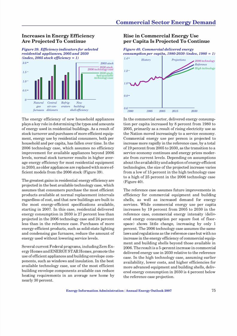
7/28/2019 2007 Annual Energy Outlook
http://slidepdf.com/reader/full/2007-annual-energy-outlook 84/243
Increases in Energy Efficiency Are Projected To Continue
Figure 39. Efficiency indicators for selected
residential appliances, 2005 and 2030
(index, 2005 stock efficiency = 1)
The energy efficiency of new household appliancesplays a key role in determining the types and amountsof energy used in residential buildings. As a result of stock turnover and purchases of more efficient equip-ment, energy use by residential consumers, both perhousehold and per capita, has fallen over time. In the2006 technology case, which assumes no efficiencyimprovement for available appliances beyond 2006levels, normal stock turnover results in higher aver-
age energy efficiency for most residential equipmentin 2030, as older appliances are replaced with more ef-ficient models from the 2006 stock (Figure 39).
The greatest gains in residential energy efficiency areprojected in the best available technology case, whichassumes that consumers purchase the most efficient
products available at normal replacement intervalsregardless of cost, and that new buildings are built tothe most energy-efficient specifications available,starting in 2007. In this case, residential deliveredenergy consumption in 2030 is 27 percent less thanprojected in the 2006 technology case and 24 percentless than in the reference case. Purchases of moreenergy-efficient products, such as solid-state lighting
and condensing gas furnaces, reduce the amount of energy used without lowering service levels.
Several current Federal programs, including Zero En-ergy Homes and ENERGY STAR Homes, promote theuse of efficient appliances and building envelope com-ponents, such as windows and insulation. In the bestavailable technology case, use of the most efficient
building envelope components available can reduceheating requirements in an average new home bynearly 30 percent.
Rise in Commercial Energy Useper Capita Is Projected To Continue
Figure 40. Commercial delivered energy
consumption per capita, 1980-2030 (index, 1980 = 1)
In the commercial sector, delivered energy consump-tion per capita increased by 8 percent from 1980 to2005, primarily as a result of rising electricity use asthe Nation moved increasingly to a service economy.Commercial energy use per person is projected toincrease more rapidly in the reference case, by a totalof 19 percent from 2005 to 2030, as the transition to a service economy continues and energy prices moder-ate from current levels. Depending on assumptions
about the availability and adoption of energy-efficienttechnologies, the size of the projected increase variesfrom a low of 15 percent in the high technology case
to a high of 25 percent in the 2006 technology case(Figure 40).
The reference case assumes future improvements in
efficiency for commercial equipment and building shells, as well as increased demand for energyservices. While commercial energy use per capita increases by 19 percent from 2005 to 2030 in thereference case, commercial energy intensity (deliv-ered energy consumption per square foot of floor-space) shows little change, increasing by only 1percent. The 2006 technology case assumes the same
laws and regulations as the reference case but with noincrease in the energy efficiency of commercial equip-ment and building shells beyond those available in2006. The result is a 5-percent increase in commercialdelivered energy use in 2030 relative to the referencecase. In the high technology case, assuming earlieravailability, lower costs, and higher efficiencies formore advanced equipment and building shells, deliv-ered energy consumption in 2030 is 4 percent belowthe reference case projection.
Energy Information Administration / Annual Energy Outlook 2007 75
Commercial Sector Energy Demand
Natural
gas
furnaces
Central
air con-
ditioners
Refrig-
erators
New
building
shell efficiency
0.0
0.5
1.0
1.5
2.0 2005 stock
2030 stock, 2006 technology case
2030 stock,best available
technology case
1980 1995 2005 2015 20300.6
0.8
1.0
1.2
1.4 History Projections 2006 technology
High technology
Reference

7/28/2019 2007 Annual Energy Outlook
http://slidepdf.com/reader/full/2007-annual-energy-outlook 85/243
Electricity Leads Expected Growthin Commercial Energy Use
Figure 41. Commercial delivered energy
consumption by fuel, 2005, 2015, and 2030
(quadrillion Btu)
Commercial floorspace growth and, in turn, commer-cial energy use are driven by trends in economic andpopulation growth. In the AEO2007 projections,growth in disposable income leads to increased de-mand for services from hotels, restaurants, stores,theaters, galleries, arenas, and other commercial es-tablishments, which in turn are increasingly depend-ent on electricity both for basic services and forbusiness services and customer transactions. In addi-
tion, the growing share of the population over age 65increases demand for healthcare and assisted living facilities and for electricity to power medical and
monitoring equipment in those facilities. The refer-ence case projects further increases in commercialelectricity use, averaging 2.0 percent per year from2005 to 2030 (Figure 41). The high and low economicgrowth cases provide high and low ranges for the av-erage annual growth rate of commercial electricity
demand from 2005 to 2030, at 2.3 percent and 1.6 per-cent, respectively.
For commercial natural gas use (primarily for spaceheating and water heating), the reference case pro-
jects average annual growth of 1.3 percent from 2005
to 2030, and for liquid fuels use the projected averageannual growth rate is 0.2 percent. The alternativeprojections for natural gas use in 2030 range from a high of 4.7 quadrillion Btu in the high growth case to4.0 in the low growth case, compared with 4.4 in thereference case. For liquid fuels use, the low and highoil price cases provide high and low estimates, respec-tively, which in 2030 vary by 0.2 and 0.1 quadrillionBtu from the reference case projection of 0.8 quadril-lion Btu.
Current Technologies ProvidePotential Energy Savings
Figure 42. Efficiency indicators for selected
commercial energy end uses, 2005 and 2030
(index, 2005 stock efficiency = 1)
The stock efficiency of energy-using equipment in thecommercial sector increases in the AEO2007 refer-ence case. Adoption of more energy-efficient equip-ment is expected to moderate the projected growth indemand, in part because of building codes for newconstruction and minimum efficiency standards, in-cluding those in EPACT2005; however, the long ser-vice lives of many kinds of energy-using equipmentlimit the pace of efficiency improvements.
The most rapid increase in overall energy efficiencyfor the commercial sector is projected in the best tech-
nology case, which assumes that only the most effi-cient technologies are chosen, regardless of cost, andthat building shells in 2030 are 50 percent more effi-cient than projected in the reference case. With the
adoption of improved heat exchangers for space heat-ing and cooling equipment, solid-state lighting, andmore efficient compressors for commercial refrigera-tion, commercial delivered energy consumption in2030 in the best technology case is 13 percent lessthan projected in the reference case and 17 percentless than in the 2006 technology case.
In the 2006 technology case, which assumes equip-
ment and building shell efficiencies limited to thoseavailable in 2006, energy efficiency in the commercialsector still is projected to improve from 2005 to 2030(Figure 42), because the technologies available in2006 can provide savings relative to commercialequipment currently in place. When businesses con-sider equipment purchases, however, the additional
capital investment needed to buy the most efficienttechnologies often carries more weight than do futureenergy savings.
76 Energy Information Administration / Annual Energy Outlook 2007
Commercial Sector Energy Demand
Electricity Natural gas Liquid fuels0
2
4
6
8 2005
2030
2015
Natural
gas
heating
Electric
cooling
Light-
ing
Refrigera-
tion
0.0
0.5
1.0
1.5
2.0
2.5 2005 stock
2030 stock, 2006 technology case
2030 stock,best available
technology case

7/28/2019 2007 Annual Energy Outlook
http://slidepdf.com/reader/full/2007-annual-energy-outlook 86/243
Advanced Technologies Could Slow Electricity Consumption in Buildings
Figure 43. Buildings sector electricity generation
from advanced technologies, 2030
(percent change from reference case)
Alternative technology cases for the residential andcommercial sectors vary the assumptions aboutavailability and market penetration of distributedgeneration technologies. In the high technology case,buildings generate 6.2 billion kilowatthours (38 per-cent) more electricity in 2030 than the 16.1 billionkilowatthours projected in the reference case (Figure43), most of which offsets residential and commercialelectricity purchases. In the best available technology
case, electricity generation in buildings in 2030 is 27.4billion kilowatthours (171 percent) higher than in thereference case, with solar systems responsible for 78
percent of the increase. The optimistic assumptionsof the best technology case benefit solar PV systemsin particular, because there are no fuel expenses forsolar systems. In the 2006 technology case, assuming no technological progress or cost reductions after2006, electricity generation in buildings in 2030 is 6.1
billion kilowatthours (38 percent) lower than in thereference case.
Some of the heat produced by fossil-fuel-fired gener-ating systems may be used to satisfy heating needs inCHP applications, increasing system efficiency and
enhancing the attractiveness of distributed genera-tion technologies for buildings. On the other hand,additional natural gas use for distributed generationsystems in the high technology and best technologycases offsets some of the energy cost reductions thatresult from improvements in end-use equipmentand building shells. In addition, if natural gas pricesincreased substantially, commercial establishmentscould find electricity purchases more economicalthan the installation of distributed generation
technologies.
Economic Growth Cases Show Rangefor Projected Industrial Energy Use
Figure 44. Industrial delivered energy consumption,
1980-2030 (quadrillion Btu)
In the AEO2007 projections, the path of industrial de-livered energy consumption varies significantly, de-pending on the assumptions used in different cases.The projections for industrial sector energy consump-tion in 2030 range from 26.0 quadrillion Btu in thelow economic growth case to 35.3 quadrillion Btu inthe high growth case, with the reference case projec-tion approximately midway between the two at 30.5quadrillion Btu (Figure 44).
In the refining industry, reliance on nonconventionalinputs for liquid fuels production is projected to in-
crease rapidly. As a result, energy consumption by re-fineries in the reference case increases from 3.7quadrillion Btu in 2005 to 6.3 quadrillion Btu in 2030.More than 60 percent of the increase is the result of
increased coal use for CTL production and biomassuse for ethanol production.
Non-fuel uses of energy transform normal energy in-puts into other, non-energy products. In 2005, theU.S. chemical industry converted petroleum productswith an estimated energy value of 3.4 quadrillion Btu
into products such as plastics and fertilizers. Suchnon-fuel use is projected to increase in the reference
case, to 3.9 quadrillion Btu in 2030. In addition, pe-troleum use to make asphalt and road oil, which arenecessary components of construction industry activ-ities, is projected to increase from 1.3 quadrillion Btuin 2005 to 1.4 quadrillion Btu in 2030. If energy con-sumption in the refining sector were excluded, non-fuel uses of petroleum would account for all the pro-
jected increase in industrial sector petroleum use inthe reference case.
Energy Information Administration / Annual Energy Outlook 2007 77
Industrial Sector Energy Demand
Distributed
generation
(all technologies)
Photo-
voltaics
Fuel
cells
Microturbines0
250
500
750
Best available technology High tech nology
1980 1995 2005 2015 20300
10
20
30
40 History Projections
Low growth
High growth
Reference

7/28/2019 2007 Annual Energy Outlook
http://slidepdf.com/reader/full/2007-annual-energy-outlook 87/243
Energy-Intensive Industries Grow Less Rapidly Than Industrial Average
Figure 45. Average output growth in the
manufacturing subsectors, 2005-2030
(percent per year)
One of the most important determinants of industrialsector energy consumption is growth in value of ship-ments. In AEO2007 , average annual growth in valueof shipments for the industrial sector from 2005 to2030 ranges from 1.2 percent per year in the low eco-nomic growth case to 2.8 percent per year in the highgrowth case, with the reference case projection ap-proximately midway between the two at 2.0 percentper year. The range of growth in the individual
subsectors is even wider.
By manufacturing subsector, the projected rate of
growth in value of shipments in the reference caseranges from a low of 0.6 percent per year (wood prod-ucts) to a high of 4.6 percent per year (computers). Ingeneral, the projected growth rates for the energy-
intensive manufacturing subsectors are lower thanthose for the non-energy-intensive subsectors. Glassis the only energy-intensive subsector with a pro-
jected growth rate above 2 percent per year in the ref-erence case.
The projected growth rates for value of shipments in
the industrial subsectors in the high and loweconomic growth cases generally are symmetrical
around the reference case (Figure 45). Industrieswith the most rapid projected growth in the referencecase show the widest ranges, so that the pattern of faster value of shipments growth for the non-energy-intensive manufacturing sectors in the reference caseis also evident in the high and low economic cases.
Energy Consumption Growth Varies Widely Across Industry Sectors
Figure 46. Average growth of delivered energy
consumption in the manufacturing subsectors,
2005-2030 (percent per year)
The average annual growth rate for total deliveredenergy consumption in the industrial sector from2005 to 2030 ranges from an increase of 0.2 percentper year to an increase of 1.4 percent per year in thealternative cases for AEO2007 . The widest variationis across the economic growth cases. Again, the rangeof the projections for individual subsectors is wider.
In the reference case, energy consumption growthrates for the manufacturing subsectors range from anincrease of 3.0 percent per year (computers andelectronics) to a decrease of 0.5 percent per year (alu-
minum). Delivered energy consumption growth insome of the energy-intensive industries (aluminumand steel) is held down by expected changes in pro-duction technology over the projection period. In gen-
eral, the subsectors with the highest projected growthrates in energy consumption are those with the high-est projected growth rates in value of shipments (com-puters and glass). The petroleum refining sector is anexception. As more refineries shift to alternativefeedstocks for liquids production (biomass, coal,heavier crude oil) they use more energy per unit of output than is used for traditional petroleum-based
refining.The projected rates of growth in energy consumptionin the alternative economic growth cases are gener-ally symmetric around the reference case (Figure 46);however, the rate of growth is moderated by the levelof investment in each case.
78 Energy Information Administration / Annual Energy Outlook 2007
Industrial Sector Energy Demand
Energy-intensive Food
Paper Petroleum refineries
Bulk chemicalsGlass
Cement Iron and steel
Aluminum
Non-energy-intensive Fabricated metals
MachineryComputers and electronicsTransportation equipment
Electrical equipmentWood products
Plastics and rubber products Balance of manufacturing
0.0 1.0 2.0 3.0 4.0 5.0 6.0-1.0
Reference High growth
Low growt h
Energy-intensive Food
Paper Petroleum refineries
Bulk chemicalsGlass
Cement Iron and steel
Aluminum
Non-energy-intensive Fabricated metals
MachineryComputers and electronicsTransportation equipment
Electrical equipmentWood products
Plastics and rubber products Balance of manufacturing
0.0 1.0 2.0 3.0 4.0 5.0-1.0-2.0
Reference High growth
Low growth

7/28/2019 2007 Annual Energy Outlook
http://slidepdf.com/reader/full/2007-annual-energy-outlook 88/243
Energy Intensity in the IndustrialSector Continues To Decline
Figure 47. Industrial delivered energy intensity,
1980-2030 (thousand Btu per 2000 dollar
value of shipments)
From 1980 to 2004 [162], energy consumption in theindustrial sector was virtually unchanged, growing bya total of 3.1 percent, while value of shipments in-creased by 50 percent. Thus, industrial delivered en-ergy use per dollar of industrial value of shipmentsdeclined by an average of 1.6 percent per year from1980 to 2004 (Figure 47). Since 1990, however, therate of decline in the sector’s energy intensity hasslowed: a 29-percent increase in industrial output
from 1990 to 2004 resulted in a 6.5-percent increasein energy use and a 1.4-percent average annual de-cline in energy intensity.
Factors contributing to the decline in industrialenergy intensity include a greater focus on energyefficiency after the energy price shocks of the 1970s
and 1980s and a reduction in the share of industrialactivity accounted for by the most energy-intensiveindustries. The energy-intensive industries’ share of industrial output fell from 24 percent in 1980 to 21percent in 2004.
The industrial value of shipments is projected to grow
by 65 percent overall from 2005 to 2030, and theshare attributed to the energy-intensive industries is
projected to fall from 20 percent in 2005 to 17 percentin 2030. Consequently, even if no specific industryshowed a reduction in energy intensity, the aggregateenergy intensity of the industrial sector as a wholewould decline [163].
Expected Declines in Energy Intensity Vary by Industry and Technology
Figure 48. Average change in energy intensity
in the manufacturing subsectors, 2005-2030
(percent per year)
Energy intensity in the industrial subsectors canchange for a variety of reasons. For example, no newprimary smelting capacity is expected to be con-structed in the U.S. aluminum industry, and second-ary smelting, a less energy-intensive process of melting scrap, is expected to become the subsector‘sdominant technology. As a result, the reference caseprojection for energy intensity in the aluminum in-dustry in 2030 is nearly one-third less than the 2005
level. In the petroleum refining industry, projectedincreases in coal use for CTL production result in in-creasing energy intensity, at an average rate of 1.0
percent per year from 2005 to 2030 [164].
A range of potential energy intensity and energy con-sumption outcomes for the industrial sector were
developed for AEO2007 . Energy intensity in the re-fining industry does not change in the 2006 tech-nology and high technology cases [165 ]. Excluding refineries, projected average annual decreases in ag-gregate industrial energy intensity range from 1.0percent per year in the 2006 technology case to 1.7percent per year in the high technology case (Figure48). In the high technology case, industrial delivered
energy consumption in 2030 (excluding refining) is1.4 quadrillion Btu less than in the reference case forthe same level of output; in the 2006 technology case,it is 2.9 quadrillion Btu higher than in the referencecase. Although the energy efficiency of new equip-ment is assumed to remain at 2006 levels in the 2006technology case, average efficiency improves as oldequipment is retired.
Energy Information Administration / Annual Energy Outlook 2007 79
Industrial Sector Energy Demand
Energy-intensive Food
Paper Petroleum refineries
Bulk chemicalsGlass
Cement Iron and steel
Aluminum
Non-energy-intensive Fabricated metals
MachineryComputers and electronicsTransportation equipment
Electrical equipmentWood products
Plastics and rubber products Balance of manufacturing
0.0 0.5 1.0-0.5 -1.0-1.5 -2.0-2.5
Reference 2006 technology
High technology
1980 1995 2004 2015 20300
2
4
6
8 History Projections
2006 technology
High technology Reference

7/28/2019 2007 Annual Energy Outlook
http://slidepdf.com/reader/full/2007-annual-energy-outlook 89/243
Transportation Energy UseIs Expected To Increase
Figure 49. Delivered energy consumption for
transportation, 1980-2030 (quadrillion Btu)
Total delivered energy consumption in the transpor-tation sector is projected to grow at an average annualrate of 1.4 percent in the AEO2007 reference case,from 28.1 quadrillion Btu in 2005 to 39.3 quadrillionBtu in 2030 (Figure 49). The reference case projectionis consistent with recent historical trends.
Energy demand for transportation is influenced by a
variety of factors, including economic growth, popula-tion growth, fuel prices, and vehicle fuel efficiency(for example, economic growth drives energy demandfor heavy vehicle travel, and fuel prices and economic
growth drive energy demand for light-duty vehicletravel). AEO2007 provides several cases to examinethe impacts of those factors on delivered energy de-mand. In 2030, the sector’s delivered energy demand
is about 10 percent higher in the high economicgrowth case and 10 percent lower in the low economicgrowth case than projected in the reference case, andit is about 10 percent lower in the high world oil pricecase and 5 percent higher in the low oil price case thanin the reference case.
By transportation mode, the most rapid increase inthe share of total delivered energy demand for trans-
portation is projected for heavy vehicle travel, whichincludes medium and large freight trucks and buses.Energy demand for heavy vehicles accounted for 18percent of the sector’s total delivered energy demandin 2005, and in 2030 it accounts for 20 percent of thetotal in the reference case. Energy demand for airtravel accounts for 10 percent of the total in 2030, the
same as in 2005, because infrastructure constraintslimit the potential growth of air travel in the UnitedStates.
Higher Prices Slow Increase inDemand for Light-Duty Vehicle Fuels
Figure 50. Delivered energy consumption in
light-duty vehicles, 1980-2030 (quadrillion Btu)
Delivered energy consumption for light-duty vehicletravel is projected to grow at an average annual rateof 1.3 percent in the reference case, from 16.9 quadril-lion Btu in 2005 to 23.5 quadrillion Btu in 2030(Figure 50). In 1980, energy use for light-duty vehicletravel totaled 11.8 quadrillion Btu.
The two factors that have the greatest impact on en-
ergy demand for light-duty vehicles in AEO2007 arefuel price and, to a lesser extent, disposable income.The high economic growth case and high world oilprice case provide higher and lower ranges, respec-
tively, for the projections. The high growth case pro- jects 25.3 quadrillion Btu, and the high price caseprojects 20.3 quadrillion Btu, for light-duty vehicleenergy use in 2030.
The projections in the low world oil price case arenearly the same as those in the high economic growthcase. As compared with the reference case, increasedtravel demand in the high growth case results in an8-percent increase in energy use for light-duty vehi-cles in 2030; in the low price case, the combination of
lower vehicle fuel economy and higher travel demandleads to a 7-percent increase.
Energy demand for light-duty vehicle travel in 2030is lower in both the high price case and the lowgrowth case than projected in the reference case, by14 percent and 8 percent, respectively. Lower travel
demand is the chief reason for the decrease in bothcases. In addition, the high price case projects a 9-percent increase in light-duty vehicle fuel economyin 2030 relative to the reference case projection.
80 Energy Information Administration / Annual Energy Outlook 2007
Transportation Sector Energy Demand
1980 1995 2005 2015 20300
5
10
15
20
25 History Projections
Low growth
High growth Reference Low price
High price
1980 1995 2005 2015 20300
10
20
30
40
50 History Projections
Low growth
High growth
Reference Low price
High price
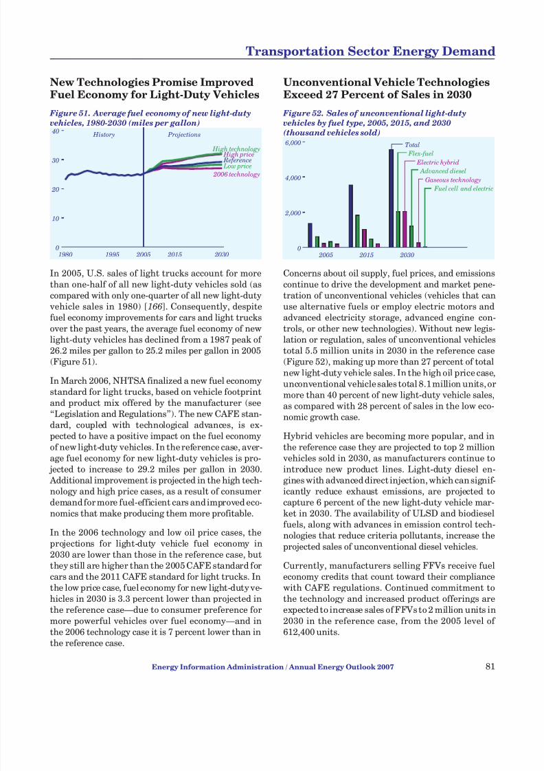
7/28/2019 2007 Annual Energy Outlook
http://slidepdf.com/reader/full/2007-annual-energy-outlook 90/243
New Technologies Promise ImprovedFuel Economy for Light-Duty Vehicles
Figure 51. Average fuel economy of new light-duty
vehicles, 1980-2030 (miles per gallon)
In 2005, U.S. sales of light trucks account for morethan one-half of all new light-duty vehicles sold (ascompared with only one-quarter of all new light-dutyvehicle sales in 1980) [166]. Consequently, despitefuel economy improvements for cars and light trucksover the past years, the average fuel economy of newlight-duty vehicles has declined from a 1987 peak of 26.2 miles per gallon to 25.2 miles per gallon in 2005(Figure 51).
In March 2006, NHTSA finalized a new fuel economystandard for light trucks, based on vehicle footprint
and product mix offered by the manufacturer (see“Legislation and Regulations”). The new CAFE stan-dard, coupled with technological advances, is ex-pected to have a positive impact on the fuel economy
of new light-duty vehicles. In the reference case, aver-age fuel economy for new light-duty vehicles is pro-
jected to increase to 29.2 miles per gallon in 2030. Additional improvement is projected in the high tech-nology and high price cases, as a result of consumerdemand for more fuel-efficient cars and improved eco-nomics that make producing them more profitable.
In the 2006 technology and low oil price cases, the
projections for light-duty vehicle fuel economy in2030 are lower than those in the reference case, butthey still are higher than the 2005 CAFE standard forcars and the 2011 CAFE standard for light trucks. Inthe low price case, fuel economy for new light-duty ve-hicles in 2030 is 3.3 percent lower than projected inthe reference case—due to consumer preference for
more powerful vehicles over fuel economy—and inthe 2006 technology case it is 7 percent lower than inthe reference case.
Unconventional Vehicle TechnologiesExceed 27 Percent of Sales in 2030
Figure 52. Sales of unconventional light-duty
vehicles by fuel type, 2005, 2015, and 2030
(thousand vehicles sold)
Concerns about oil supply, fuel prices, and emissionscontinue to drive the development and market pene-tration of unconventional vehicles (vehicles that canuse alternative fuels or employ electric motors andadvanced electricity storage, advanced engine con-trols, or other new technologies). Without new legis-lation or regulation, sales of unconventional vehiclestotal 5.5 million units in 2030 in the reference case(Figure 52), making up more than 27 percent of total
new light-duty vehicle sales. In the high oil price case,unconventional vehicle sales total 8.1 million units, ormore than 40 percent of new light-duty vehicle sales,
as compared with 28 percent of sales in the low eco-nomic growth case.
Hybrid vehicles are becoming more popular, and in
the reference case they are projected to top 2 millionvehicles sold in 2030, as manufacturers continue tointroduce new product lines. Light-duty diesel en-gines with advanced direct injection, which can signif-icantly reduce exhaust emissions, are projected tocapture 6 percent of the new light-duty vehicle mar-ket in 2030. The availability of ULSD and biodieselfuels, along with advances in emission control tech-
nologies that reduce criteria pollutants, increase theprojected sales of unconventional diesel vehicles.
Currently, manufacturers selling FFVs receive fueleconomy credits that count toward their compliancewith CAFE regulations. Continued commitment tothe technology and increased product offerings areexpected to increase sales of FFVs to 2 million units in
2030 in the reference case, from the 2005 level of 612,400 units.
Energy Information Administration / Annual Energy Outlook 2007 81
Transportation Sector Energy Demand
2005 2015 20300
2,000
4,000
6,000 Total
Gaseous technology
Advanced diesel
Flex-fuel
Electric hybrid
Fuel cell and electric
1980 1995 2005 2015 20300
10
20
30
40 History Projections
2006 technology
High technology
Reference Low price
High price

7/28/2019 2007 Annual Energy Outlook
http://slidepdf.com/reader/full/2007-annual-energy-outlook 91/243

7/28/2019 2007 Annual Energy Outlook
http://slidepdf.com/reader/full/2007-annual-energy-outlook 92/243
Early Capacity Additions Use NaturalGas, Coal Plants Are Added Later
Figure 55. Electricity generation capacity additions
by fuel type, including combined heat and power,
2006-2030 (gigawatts)
In the reference case, 292 gigawatts of new generat-ing capacity (including end-use CHP) is required by2030 to meet growth in electricity demand and to re-place inefficient, older generating plants that are re-tired. Capacity decisions depend on the costs andoperating efficiencies of different options, fuel prices,demand growth, and the availability of Federal taxcredits for investments in some technologies.
Coal-fired capacity, which typically is expensive tobuild but has relatively low operating costs, accountsfor about 54 percent of the total capacity additions
from 2006 to 2030 (Figure 55). Natural-gas-firedplants, which generally are the least expensive capac-ity to build but have comparatively high fuel costs,represent 36 percent of the projected additions. Re-
newable and nuclear plants, which have high invest-ment costs and low operating costs, account for 6percent and 4 percent of total additions, respectively.Of the 12 gigawatts of new nuclear capacity expectedby 2030, 3 gigawatts is added after the EPACT2005PTC expires in 2020.
Different fuel price paths or growth rates for electric-ity demand can affect the quantity and mix of capac-
ity additions. In the low and high price cases,variations in fuel prices have little impact on total ca-pacity additions but do affect the mix of capacitytypes. Because fuel costs are a larger share of total ex-penditures for new natural-gas-fired capacity, higherfuel prices lead to more coal-fired additions. In theeconomic growth cases, capacity additions range from
191 gigawatts in the low growth case to 398 gigawattsin the high growth case, but with similar shares forthe different generating technologies in both cases.
Least Expensive Technology Options Are Likely Choices for New Capacity
Figure 56. Levelized electricity costs for new plants,
2015 and 2030 (2005 mills per kilowatthour)
Technology choices for new generating capacity aremade to minimize cost while meeting local and Fed-eral emissions constraints. The choice of technologyfor capacity additions is based on the least expensiveoption available (Figure 56) [167 ]. The AEO2007 ref-erence case assumes a capital recovery period of 20
years. In addition, the cost of capital is based on com-petitive market rates, to account for the risks of siting new units.
Capital costs decline over time (Table 16), at ratesthat depend on the current stage of development for
each technology. For the newest technologies, capitalcosts are initially adjusted upward to reflect the opti-mism inherent in early estimates of project costs. Asproject developers gain experience, the costs are as-
sumed to decline. The decline continues at a progres-sively slower rate as more units are built. Theefficiency of new plants is also assumed to improvethrough 2015, with heat rates for advanced combinedcycle and coal gasification units declining from 6,572and 8,309 Btu per kilowatthour, respectively, in 2005to 6,333 and 7,200 Btu per kilowatthour in 2015.
Energy Information Administration / Annual Energy Outlook 2007 83
Electricity Supply
2006-
2010
2011-
2015
2016-
2020
2021-
2025
2026-
2030
0
40
80
120 Natural gas
Coal
Renewables
Nuclear
Coal Gas
combined
cycle
2015
Wind Nuclear Coal Gas
combined
cycle
2030
Wind Nuclear
0
20
40
60
80
Capital costs
Variable costs, including fuel Fixed c osts
Incremental transmission costs
Table 16. Costs of producing electricity
from new plants, 2015 and 2030
Costs
2015 2030
Advanced coal
Advanced combined
cycle Advanced
coal
Advanced combined
cycle
2005 mills per kilowatthour
Capital 32.64 12.16 28.71 11.12 Fixed 4.89 1.44 4.89 1.44Variable 14.82 37.97 16.49 41.17 Incremental
transmission 3.72 3.67 3.64 3.49
Total 56.07 55.24 53.73 57.22

7/28/2019 2007 Annual Energy Outlook
http://slidepdf.com/reader/full/2007-annual-energy-outlook 93/243
Largest Capacity Additions Expectedin the Southeast and the West
Figure 57. Electricity generation capacity
additions, including combined heat and power,
by region and fuel, 2006-2030 (gigawatts)
Most areas of the United States currently have excessgeneration capacity, but all electricity demand re-gions (see Appendix F for definitions) are expected toneed additional, currently unplanned, capacity by2030. The largest amounts of new capacity are ex-pected in the Southeast (FL and SERC) and the West(NWP, RA, and CA). In the Southeast, electricity de-mand represents a relatively large share of total U.S.electricity sales, and its need for new capacity is
greater than in other regions (Figure 57).
With natural gas prices rising in the reference case,
coal-fired plants make up most of the capacityadditions through 2030, given the assumption thatcurrent environmental policies are maintained indefi-nitely. The largest concentrations of new coal-fired
plants are in the Southeast and the West. In theSoutheast, new coal-fired plants are built in view of the size of the electricity market and the correspond-ing need for additional capacity. In the West, wherethe capacity requirement is much smaller, the choiceto build mostly coal-fired plants is based on theregion’s lower-than-average coal prices and higher-than-average natural gas prices.
Nationwide, some new natural-gas-fired plants arebuilt to maintain a diverse capacity mix or to serve asreserve capacity. Most are located in the Midwest(MAPP, MAIN, and ECAR) and Southeast (FL andSERC). The Midwest has a surplus of coal-fired gen-erating capacity and does not need to add many newcoal-fired plants. In the Southeast, natural-gas-fired
plants are needed along with coal-fired plants tomaintain diversity in the capacity mix.
EPACT2005 Tax Credits Are ExpectedTo Stimulate New Nuclear Builds
Figure 58. Electricity generation from nuclear
power, 1973-2030 (billion kilowatthours)
In the AEO2007 reference case, nuclear capacity in-creases from 100.0 gigawatts in 2005 to 112.6 giga-watts in 2030. The change includes 2.7 gigawatts of capacity expansion at existing plants, 12.5 gigawattsof capacity at new plants, and 2.6 gigawatts of retire-ments of older units. EPACT2005 provides an 8-yearPTC of 1.8 cents per kilowatthour for up to 6gigawatts of new nuclear capacity built before 2021;however, the credit can be shared for additional ca-
pacity at a lower credit value. The reference case as-sumes that 9.0 gigawatts will be built by 2020 and willreceive tax credits worth 1.2 cents per kilowatthour.
The increase in capacity at existing units assumesthat all uprates approved, pending, or expected by theNRC will be carried out.
Most existing nuclear units are expected to continueoperating through 2030, based on the assumptionthat they will apply for and receive license renewals.Four units, totaling 2.6 gigawatts, are projected tobe retired in 2030, when the date of their originallicenses plus a 20-year renewal is reached.
Projected nuclear capacity additions vary, depending on overall demand for electricity and the prices of
other fuels. Across the five main AEO2007 cases,nuclear generation grows from 780 billion kilowatt-hours in 2005 to between 799 and 1,010 billion kilo-watthours in 2030 (Figure 58). In the low price case,the delivered price of natural gas in 2030 is 10 percentlower than in the reference case, and new nuclearplants are not economical. In the high price and high
growth cases, respectively, 24 and 27 gigawatts of new nuclear capacity are projected, because more ca-pacity is needed and the cost of alternatives is higher.
84 Energy Information Administration / Annual Energy Outlook 2007
Electricity Supply
1970 1980 1995 2005 2015 20300
300
600
900
1,200 History Projections
Low growth
High growth
Reference
Low price
High price
ECAR
ERCOT
MAAC
MAIN
MAPP
NY
NE
FL
SERC
SPP
NWP
RA
CA
0 20 40 60 80
Nuclear
Natural gas
Renewable/ other
Coal

7/28/2019 2007 Annual Energy Outlook
http://slidepdf.com/reader/full/2007-annual-energy-outlook 94/243
When Lower Costs Are Assumed, New Nuclear Plants Are More Competitive
Figure 59. Levelized electricity costs for new plants
by fuel type, 2015 and 2030
(2005 cents per kilowatthour)
The reference case assumptions for the cost and per-formance characteristics of new technologies arebased on cost estimates by government and industryanalysts, allowing for uncertainties about new de-signs. Because no new nuclear plants have been or-dered in this country since 1977, there is no reliableestimate of what they might cost. To test the signifi-cance of uncertainty in the assumptions, alternativecases vary key parameters. The low nuclear cost case
assumes capital and operating costs 10 percent belowthose in the reference case in 2030, reflecting a 25-percent reduction in overnight capital costs from
2006 to 2030. The high nuclear cost case assumes nochange in capital costs for advanced nuclear technolo-gies from their 2006 levels.
Nuclear generating costs in the low nuclear cost caseare more competitive with the generating costs fornew coal- and natural-gas-fired units toward the endof the projection period (Figure 59). (The figure showsaverage generating costs, assuming generation at themaximum capacity factor for each technology; thecosts and relative competitiveness of the technologiescould vary by region.) In the reference case, Federal
tax credits result in 9.0 gigawatts of new nuclear ca-pacity by 2020, leading to lower costs in the futureand an additional 3.5 gigawatts after the tax creditsexpire. In the low nuclear cost case, 28.5 gigawatts of new nuclear capacity is added between 2005 and2030. The additional nuclear capacity displaces pri-marily new coal-fired capacity. In the high nuclearcost case, where capital costs are higher than ex-pected, only 6 gigawatts of nuclear capacity is pro-
jected to be built, all due to the Federal tax credits.
Biomass and Wind Lead ProjectedGrowth in Renewable Generation
Figure 60. Nonhydroelectric renewable electricity
generation by energy source, 2005-2030
(billion kilowatthours)
There is considerable uncertainty about the growthpotential of wind power, which depends on a varietyof factors, including fossil fuel costs, State renewableenergy programs, technology improvements, accessto transmission grids, public concerns about environ-mental and other impacts, and the future of the Fed-eral PTC, which was set to expire at the end of 2007but has been extended to 2008. In the AEO2007 refer-ence case, generation from wind power increases from
0.4 percent of total generation in 2005 to 0.9 percentin 2030 (Figure 60). Generation from geothermal fa-cilities, while increasing, is not projected to gain mar-
ket share and remains at its 2005 level of 0.4 percentof total generation in 2030, because opportunities forthe development of new sites are limited. Most of thesuitable sites, restricted mainly to Nevada and Cali-fornia, involve relatively high up-front costs and per-formance risks; and although geothermal power
plants are eligible for the Federal PTC, the long con-struction lead times required make it unlikely thatsignificant new capacity could be built in time to ben-efit from the current credit.
Among the other alternative fuel technologies, gener-
ation from municipal solid waste (MSW) and LFGstays at 0.5 percent of total generation. Solar technol-ogies in general remain too costly for grid-connectedapplications, but demonstration programs and Statepolicies support some growth in central-station solarPV, and small-scale customer-sited PV applicationsgrow rapidly [168]. Grid-connected solar generationincreases to 0.1 percent of total generation in 2030.
Energy Information Administration / Annual Energy Outlook 2007 85
Electricity Supply
2005 2010 2020 20300
50
100
150
200
250
MSW/LFG
Biomass
Wind
SolarGeothermal
Coal Natural gas
combined
cycle
Reference
case
Nuclear
Low
cost case
High
cost case
0
2
4
6
8
10
2015 2030 Variable costs, including fuel
Fixed costsCapital costs
Incremental transmission costs

7/28/2019 2007 Annual Energy Outlook
http://slidepdf.com/reader/full/2007-annual-energy-outlook 95/243
Technology Advances, Tax ProvisionsIncrease Renewable Generation
Figure 61. Grid-connected electricity generation
from renewable energy sources, 1990-2030
(billion kilowatthours)
Despite technology improvements, rising fossil fuelcosts, and public support, the contribution of renew-able fuels to U.S. electricity supply remains relativelysmall in the AEO2007 reference case at 9.0 percent of total generation in 2030—about the same as theirshare in 2005 (Figure 61). Although conventionalhydropower remains the largest source of renewablegeneration through 2030, environmental concernsand the scarcity of untapped large-scale sites limit its
growth, and its share of total generation falls from 6.6percent in 2005 to 5.3 percent in 2030. Electricitygeneration from nonhydroelectric alternative fuels
increases, however, bolstered by technology advancesand State and Federal supports. The share of nonhydropower renewable generation increases by60 percent, from 2.3 percent of total generation in2005 to 3.6 percent in 2030.
Biomass is the largest source of renewable electricitygeneration among the nonhydropower renewablefuels. Co-firing with coal is relatively inexpensivewhen low-cost biomass resources are available. Aslow-cost feedstocks begin to be exhausted, however,more costly biomass resources are used, and new ded-
icated biomass facilities, such as IGCC plants, arebuilt. Electricity generation from biomass increasesfrom 1.0 percent of total generation in 2005 to 1.8 per-cent in 2030, with approximately 47 percent of the in-crease coming from biomass co-firing, 29 percentfrom dedicated power plants, and 25 percent fromnew on-site CHP capacity.
Renewables Are Expected To BecomeMore Competitive Over Time
Figure 62. Levelized and avoided costs for new
renewable plants in the Northwest, 2030
(2005 mills per kilowatthour)
The competitiveness of both conventional and renew-able generation resources is based on the most cost-effective mix of capacity that satisfies the demand forelectricity across all hours and seasons. Baseloadtechnologies tend to have low operating costs and setthe market price for power only during the hours of least demand. Dispatchable geothermal and biomassresources compete directly with new coal and nuclearplants, which to a large extent determine the avoided
cost [169] for baseload energy. In some regions and years, new geothermal or biomass plants may be com-petitive with new coal-fired plants, but their develop-
ment is limited by the availability of geothermalresources or competitive biomass fuels.
Wind and solar are intermittent technologies that can
be used only when resources are available. With rela-tively low operating costs and limited resource avail-ability, their avoided costs are determined largely bythe operating costs of the most expensive units in op-eration when their resources are available. Solar gen-erators tend to operate during peak load periods,when natural-gas-fired combustion turbines andcombined-cycle units with higher fuel costs deter-
mine avoided costs. The levelized cost of solar ther-mal generation is significantly higher than its avoidedcost through 2030 (Figure 62). The availability of wind resources varies among regions, but wind plantstend to displace intermediate load generation. Thus,the avoided costs of wind power are determinedlargely by the low-to-moderate operating costs of combined-cycle and coal-fired plants, which set powerprices during intermediate load hours. In some re-gions and years, levelized costs for wind power are ap-
proximately equal to its avoided costs.
86 Energy Information Administration / Annual Energy Outlook 2007
Electricity Supply
GeothermalSolar thermal
BiomassWind
GeothermalSolar thermal
BiomassWind
GeothermalSolar thermal
BiomassWind
0 50 100 150 200
Levelized cost Avoided cost
Reference
Low renewables
High renewables
1990 2000 2005 2010 2020 20300
100
200
300
400
Conventional
hydropower
Other
renewables
History Projections

7/28/2019 2007 Annual Energy Outlook
http://slidepdf.com/reader/full/2007-annual-energy-outlook 96/243
State Portfolio Standards IncreaseGeneration from Renewable Fuels
Figure 63. Renewable electricity generation,
2005-2030 (billion kilowatthours)
In 2005, 23 States and the District of Columbia hadRPS or similar programs in effect. An alternative casewas prepared for AEO2007 to examine the potentialimpacts of full compliance with those programs. Be-cause NEMS does not provide projections at the Statelevel, the AEO2007 regional RPS case assumed thatall States would reach their goals within each pro-gram’s legislative framework, and the results wereaggregated at the regional level. In some States, how-
ever, compliance could be limited by authorized fund-ing levels for the programs. For example, California isnot expected to meet its renewable energy targets
because of restraints on the funding of its RPSprogram.
In the regional RPS case, State renewable energy pro-
grams are projected to result in a national total of 61billion kilowatthours of additional nonhydropowerrenewable generation in 2030 relative to the refer-ence case, a 29-percent increase (Figure 63). Most of the additional generation is projected to come frombiomass resources, with smaller increases for wind,municipal waste, and geothermal generation, whichtogether account for 8 percent of the projected
increase.Nearly 5 gigawatts of additional new dedicated bio-mass capacity is projected for the mid-Atlantic regionin the RPS case, as a result of the implementation of aggressive standards and the limited availability of other renewable resources. Florida, New York, andNew England each would add 500 megawatts or more
biomass capacity, whereas States in the West wouldadd little new capacity beyond that projected in thereference case.
Fossil-Fired Capacity Additions Vary With Cost and Performance
Figure 64. Cumulative new generating capacity by
technology type, 2006-2030 (gigawatts)
The cost and performance of various generating tech-nologies in the reference case are determined in con-sultation with industry and government specialists.To test the significance of uncertainty in the assump-tions, alternative cases vary key parameters. In thehigh fossil technology case, capital costs, heat rates,and operating costs for advanced fossil-fired generat-ing technologies in 2030 are assumed to be 10 percentlower than in the reference case. The low fossil tech-
nology case assumes no change from the 2006 capitalcosts and heat rates for advanced technologies.
With different cost and performance assumptions,the mix of generating technologies changes (Figure64). In all cases, assuming continuation of current en-vironmental policies, coal technologies account for at
least 50 percent of new capacity additions; in the highfossil technology case, 70 percent of coal-fired addi-tions use advanced technologies, compared with only2 percent in the low fossil case. Natural-gas-fired ca-pacity makes up 35 to 42 percent of new additions inall cases. Advanced technologies represent 72 percentof those additions in the high fossil case and 55 per-cent in the low fossil case. The improved economics of
advanced fossil technologies in the high fossil case re-sult in fewer nuclear and renewable builds and moreretirements of older steam units. Electricity pricesare 2 percent lower in 2030 in the high fossil case thanin the reference case. Because fossil-fired capacity ismore costly in the low fossil case, more nuclear capac-ity (11 gigawatts) and slightly more renewable capac-ity are added; however, the higher costs of operating less efficient fossil-fired capacity in the low fossil tech-nology case cause projected electricity prices in 2030
to be 2 percent higher than in the reference case.
Energy Information Administration / Annual Energy Outlook 2007 87
Electricity Supply
2005 2010 2015 2020 2025 20300
50
100
150
200
250
Reference
Regional RPS
Low fossil Reference High fossil0
50
100
150
200
250 Coal
Natural gas
Advanced coal
Renewable/
Advanced gas
Nuclear other

7/28/2019 2007 Annual Energy Outlook
http://slidepdf.com/reader/full/2007-annual-energy-outlook 97/243
Fuel Costs Drop from Recent Highs,Then Increase Gradually
Figure 65. Fuel prices to electricity generators,
1995-2030 (2005 dollars per million Btu)
Electricity production costs are a function of fuel,operation and maintenance, and capital costs. In thereference case, fuel costs account for about two-thirdsof production costs for new natural-gas-fired plants,less than one-third for new coal-fired units, and aboutone-tenth for new nuclear power plants in 2030.Generation from natural-gas-fired power plants in-creased in the early 2000s, but rising natural gasprices have increased their generation costs. After a
34-percent jump from 2004, natural gas prices were$8.18 per million Btu (2005 dollars) in 2005.
In the reference case, the price of natural gas deliv-ered to the electric power sector drops to $5.50 permillion Btu in 2013, then rises to $6.33 per millionBtu in 2030 (Figure 65). Coal prices to the electric
power sector remain relatively low, peaking at $1.71per million Btu in 2010, falling to $1.69 per millionBtu in 2018, and remaining at that level through2030. Accordingly, the natural gas share of genera-tion (including utilities, independent power produc-ers, and end-use CHP) peaks at 22 percent in 2016,then drops to 16 percent in 2030 as prices rise, whilethe coal share increases from 50 percent in 2016 to 57
percent in 2030. Nuclear fuel costs rise steadily, to$0.62 per million Btu in 2030.
In the low and high price cases, coal prices to thepower sector in 2030 are $1.51 and $1.80 per millionBtu, respectively, and natural gas prices are $5.71and $7.79 per million Btu. As a result, the respectivecoal and natural gas shares of total generation in 2030
are projected to be 45 percent and 27 percent in thelow price case, as compared with 61 percent and 11percent in the high price case.
Electricity Prices Moderate in theNear Term, Then Rise Gradually
Figure 66. Average U.S. retail electricity prices,
1970-2030 (2005 cents per kilowatthour)
In the reference case, retail electricity prices peak at8.3 cents per kilowatthour (2005 dollars) in 2006,then fall to 7.7 cents per kilowatthour in 2015 as newsources of natural gas and coal are brought on line.
After 2013, fossil fuel prices rise slowly but steadily,and retail electricity prices also rise gradually after2015, to 8.1 cents per kilowatthour in 2030 (Figure66). Customers in States with competitive retail mar-kets for electricity are expected to see the effects of
changes in natural gas prices in their electricity billsmore rapidly than those in regulated States, becausecompetitive prices are determined by the marginal
cost of energy rather than the average of all plantcosts, and natural-gas-fired plants, with their higheroperating costs, often set hourly marginal prices.
Electricity distribution costs are projected to declineby 8 percent from 2005 to 2030, as technology im-provements and a growing customer base lower thecost of the distribution infrastructure. Transmissioncosts, on the other hand, increase by 29 percent,because additional investment is needed to meet con-sumers’ growing demand for electricity and to facili-tate competition in wholesale energy markets.
Economic expansion increases electricity consump-tion by businesses, factories, and residents as theybuy and use more electrical equipment. Thus, overthe long term, the rate of economic growth has a greater effect on the range of electricity prices than dooil and natural gas prices, because power supplierscan substitute coal, nuclear, and renewable fuels for
expensive natural gas. In the low and high economicgrowth cases, electricity prices are 7.8 and 8.4 centsper kilowatthour, respectively, in 2030.
88 Energy Information Administration / Annual Energy Outlook 2007
Electricity Prices
1970 1985 1995 2005 2015 20300
2
4
6
8
10
12 History Projections
1970 2030
Average price
(nominal cents)13.0
1.7
1995 2005 2010 2015 2020 2025 20300
2
4
6
8
10
Coal
Natural gas
History Projections
Liquid fuels
Nuclear

7/28/2019 2007 Annual Energy Outlook
http://slidepdf.com/reader/full/2007-annual-energy-outlook 98/243
Projected Natural Gas Use forElectricity Generation Peaks in 2020
Figure 67. Natural gas consumption by sector,
1990-2030 (trillion cubic feet)
Total natural gas consumption in the United States isprojected to increase from 22.0 trillion cubic feet in2005 to 26.1 trillion cubic feet in 2030 in the AEO2007 reference case. Much of the growth is ex-pected before 2020, with demand for natural gas inthe electric power sector growing from 5.8 trillion cu-bic feet in 2005 to a peak of 7.2 trillion cubic feet in2020 (Figure 67). Natural gas use in the electricpower sector declines after 2020, to 5.9 trillion cubic
feet in 2030, as new coal-fired generating capacitydisplaces natural-gas-fired generation. Much of theprojected decline in natural gas consumption for elec-
tricity generation results from higher delivered pricesfor natural gas in the reference case projection after2020.
Continued growth in residential, commercial, and in-dustrial consumption of natural gas is roughly offsetby the projected decline in natural gas demand forelectricity generation. As a result, overall natural gasconsumption is almost flat between 2020 and 2030 inthe AEO2007 reference case, and the natural gasshare of total projected energy consumption dropsfrom 23 percent in 2005 to 20 percent in 2030.
Natural Gas Consumption Varies withFuel Prices and Economic Growth
Figure 68. Total natural gas consumption,
1990-2030 (trillion cubic feet)
In the AEO2007 projections, domestic natural gasconsumption is influenced by the level of natural gasprices and the rate of economic growth. Higher (orlower) natural gas prices reduce (or increase) con-sumption, while higher (or lower) rates of economicgrowth increase (or reduce) gas consumption. Thegreatest variation occurs in the high and low pricecases, where natural gas consumption in 2030 rangesfrom 29.7 trillion cubic feet in the low price case to
24.1 trillion cubic feet in the high price case (Figure68). The high and low economic growth cases projectnatural gas consumption in 2030 at 28.4 trillion cubic
feet and 24.2 trillion cubic feet, respectively.
The effects of economic growth on natural gas con-sumption are not as large as the effects of prices,
because only a part of the incremental change in dis-posable personal income in the high and low economicgrowth cases is directed toward energy purchases.For example, when higher GDP growth is assumed,energy purchases make up a smaller proportions of GDP and of personal expenditures.
In contrast, the price of natural gas directly affectsthe level of natural gas consumption. High prices pro-
vide a direct economic incentive for users to reducetheir natural gas consumption, and low prices encour-age more consumption. The strength of the relation-ship between natural gas prices and consumptiondepends on the short- and long-term capabilities forfuel conservation and substitution in each consuming sector.
Energy Information Administration / Annual Energy Outlook 2007 89
Natural Gas Demand
1990 2000 2005 2010 2020 20300
2
4
6
8
10
12
Residential
Commercial
Industrial
History Projections
Electricity generators
Transportation
1990 2000 2005 2010 2020 20300
10
20
30
40 History Projections
Low growth
High growth Reference
Low price
High price
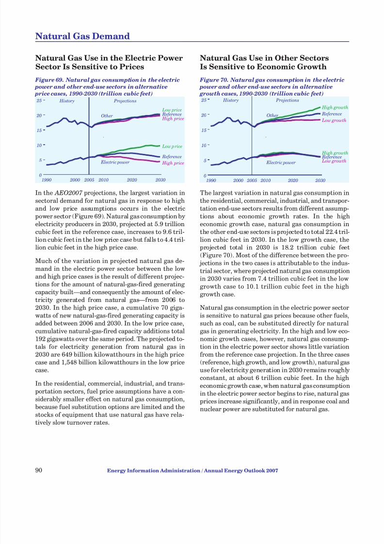
7/28/2019 2007 Annual Energy Outlook
http://slidepdf.com/reader/full/2007-annual-energy-outlook 99/243
Natural Gas Use in the Electric PowerSector Is Sensitive to Prices
Figure 69. Natural gas consumption in the electric
power and other end-use sectors in alternative
price cases, 1990-2030 (trillion cubic feet)
In the AEO2007 projections, the largest variation insectoral demand for natural gas in response to highand low price assumptions occurs in the electricpower sector (Figure 69). Natural gas consumption byelectricity producers in 2030, projected at 5.9 trillioncubic feet in the reference case, increases to 9.6 tril-lion cubic feet in the low price case but falls to 4.4 tril-lion cubic feet in the high price case.
Much of the variation in projected natural gas de-mand in the electric power sector between the lowand high price cases is the result of different projec-
tions for the amount of natural-gas-fired generating capacity built—and consequently the amount of elec-tricity generated from natural gas—from 2006 to2030. In the high price case, a cumulative 70 giga-
watts of new natural-gas-fired generating capacity isadded between 2006 and 2030. In the low price case,cumulative natural-gas-fired capacity additions total192 gigawatts over the same period. The projected to-tals for electricity generation from natural gas in2030 are 649 billion kilowatthours in the high pricecase and 1,548 billion kilowatthours in the low pricecase.
In the residential, commercial, industrial, and trans-portation sectors, fuel price assumptions have a con-siderably smaller effect on natural gas consumption,because fuel substitution options are limited and thestocks of equipment that use natural gas have rela-tively slow turnover rates.
Natural Gas Use in Other SectorsIs Sensitive to Economic Growth
Figure 70. Natural gas consumption in the electric
power and other end-use sectors in alternative
growth cases, 1990-2030 (trillion cubic feet)
The largest variation in natural gas consumption inthe residential, commercial, industrial, and transpor-tation end-use sectors results from different assump-tions about economic growth rates. In the higheconomic growth case, natural gas consumption inthe other end-use sectors is projected to total 22.4 tril-lion cubic feet in 2030. In the low growth case, theprojected total in 2030 is 18.2 trillion cubic feet(Figure 70). Most of the difference between the pro-
jections in the two cases is attributable to the indus-trial sector, where projected natural gas consumptionin 2030 varies from 7.4 trillion cubic feet in the low
growth case to 10.1 trillion cubic feet in the highgrowth case.
Natural gas consumption in the electric power sector
is sensitive to natural gas prices because other fuels,such as coal, can be substituted directly for naturalgas in generating electricity. In the high and low eco-nomic growth cases, however, natural gas consump-tion in the electric power sector shows little variationfrom the reference case projection. In the three cases(reference, high growth, and low growth), natural gasuse for electricity generation in 2030 remains roughly
constant, at about 6 trillion cubic feet. In the higheconomic growth case, when natural gas consumptionin the electric power sector begins to rise, natural gasprices increase significantly, and in response coal andnuclear power are substituted for natural gas.
90 Energy Information Administration / Annual Energy Outlook 2007
Natural Gas Demand
1990 2000 2005 2010 2020 20300
5
10
15
20
25 History Projections
High price
Low p rice
Reference
Low price
High price
Reference
Electric power
Other
1990 2000 2005 2010 2020 20300
5
10
15
20
25 History Projections
Low growth
High growth Reference
High growth
Low growth
Reference
Electric power
Other
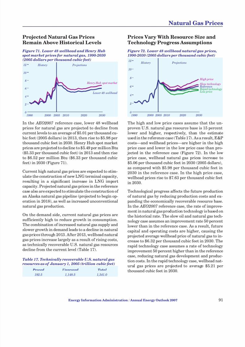
7/28/2019 2007 Annual Energy Outlook
http://slidepdf.com/reader/full/2007-annual-energy-outlook 100/243
Projected Natural Gas PricesRemain Above Historical Levels
Figure 71. Lower 48 wellhead and Henry Hub
spot market prices for natural gas, 1990-2030
(2005 dollars per thousand cubic feet)
In the AEO2007 reference case, lower 48 wellheadprices for natural gas are projected to decline fromcurrent levels to an average of $5.01 per thousand cu-bic feet (2005 dollars) in 2013, then rise to $5.98 perthousand cubic feet in 2030. Henry Hub spot marketprices are projected to decline to $5.49 per million Btu($5.33 per thousand cubic feet) in 2013 and then riseto $6.52 per million Btu ($6.33 per thousand cubicfeet) in 2030 (Figure 71).
Current high natural gas prices are expected to stim-ulate the construction of new LNG terminal capacity,
resulting in a significant increase in LNG importcapacity. Projected natural gas prices in the referencecase also are expected to stimulate the construction of an Alaska natural gas pipeline (projected to begin op-
eration in 2018), as well as increased unconventionalnatural gas production.
On the demand side, current natural gas prices aresufficiently high to reduce growth in consumption.The combination of increased natural gas supply andslower growth in demand leads to a decline in natural
gas prices through 2013. After 2013, wellhead naturalgas prices increase largely as a result of rising costs,
as technically recoverable U.S. natural gas resourcesdecline from the current level (Table 17).
Prices Vary With Resource Size andTechnology Progress Assumptions
Figure 72. Lower 48 wellhead natural gas prices,
1990-2030 (2005 dollars per thousand cubic feet)
The high and low price cases assume that the un-proven U.S. natural gas resource base is 15 percentlower and higher, respectively, than the estimateused in the reference case (Table 17). As a result, E&Pcosts—and wellhead prices—are higher in the highprice case and lower in the low price case than pro-
jected in the reference case (Figure 72). In the lowprice case, wellhead natural gas prices increase to$5.06 per thousand cubic feet in 2030 (2005 dollars),
as compared with $5.98 per thousand cubic feet in2030 in the reference case. In the high price case,wellhead prices rise to $7.63 per thousand cubic feet
in 2030.
Technological progress affects the future productionof natural gas by reducing production costs and ex-
panding the economically recoverable resource base.In the AEO2007 reference case, the rate of improve-ment in natural gas production technology is based onthe historical rate. The slow oil and natural gas tech-nology case assumes an improvement rate 50 percentlower than in the reference case. As a result, futurecapital and operating costs are higher, causing theprojected average wellhead price of natural gas to in-
crease to $6.32 per thousand cubic feet in 2030. Therapid technology case assumes a rate of technologyimprovement 50 percent higher than in the referencecase, reducing natural gas development and produc-tion costs. In the rapid technology case, wellhead nat-ural gas prices are projected to average $5.21 perthousand cubic feet in 2030.
Energy Information Administration / Annual Energy Outlook 2007 91
Natural Gas Prices
1990 2000 2005 2010 2020 20300
2
4
6
8
10
12 History Projections
High price
Rapid technology
Slow technology
Low price
Reference
1990 2000 2005 2010 2020 20300
2
4
6
8
10
12 History Projections
Henry Hub spot market
Lower 48 wellhead
Table 17. Technically recoverable U.S. natural gas
resources as of January 1, 2005 (trillion cubic feet)
Proved Unproved Total
192.5 1,148.5 1,341.0

7/28/2019 2007 Annual Energy Outlook
http://slidepdf.com/reader/full/2007-annual-energy-outlook 101/243
Delivered Natural Gas Prices Follow Trends in Wellhead Prices
Figure 73. Natural gas prices by end-use sector,
1990-2030 (2005 dollars per thousand cubic feet)
Trends in delivered natural gas prices largely reflectchanges in projected wellhead prices. In the AEO2007
reference case, prices for natural gas delivered to theend-use sectors decline through 2015 as wellhead gasprices decline, then increase along with wellheadprices over the rest of the projection period (Figure73).
On average, projected end-use transmission and dis-tribution margins remain relatively constant, be-cause the cost of adding new facilities largely offsetsthe reduced depreciation expenses of existing facili-
ties. Transmission and distribution margins in theend-use sectors reflect both the volumes of naturalgas delivered and the infrastructure arrangements of the different sectors. The industrial and electricity
generation sectors have the lowest end-use prices,because they receive most of their natural gas directlyfrom interstate pipelines, avoiding local distributioncharges. In addition, summer-peaking electricity gen-erators reduce transmission costs by using interrupt-ible transportation services during the summer,when there is spare pipeline capacity. As power gener-ators take a larger share of the natural gas market,
however, they are expected to rely more on highercost firm transportation service.
The reference case assumes that sufficient trans-mission and distribution capacity will be built toaccommodate the projected growth in natural gasconsumption. If public opposition were to preventinfrastructure expansion, however, delivered prices
could be higher than projected in the reference case.
Transmission and Distribution Costs Are Reduced With Higher Volumes
Figure 74. Average natural gas transmission and
distribution margins, 1990-2030
(2005 dollars per thousand cubic feet)
The transmission and distribution margin for naturalgas delivered to end users is the difference betweenthe average delivered price and the average sourceprice, which is the quantity-weighted average of thelower 48 wellhead price and the average import price.It reflects both the capital and operating costs forpipelines and the volume of natural gas transported.
Although operating costs vary with the level of pipe-line utilization, capital costs are fixed for the most
part. Variations in pipeline throughput result inhigher or lower transmission and distribution costsper thousand cubic feet of natural gas transported.
Thus, because the high and low price case projectionsshow the greatest variation in total natural gas con-sumption, the greatest variation in transmission anddistribution margins is also seen in those cases.
In the high price case, total natural gas consumptionin 2030 is projected to be only 24.1 trillion cubic feet.
As a result, the average transmission and distributionmargin for delivered natural gas is projected to in-crease from $2.38 per thousand cubic feet in 2005 to$2.44 per thousand cubic feet in 2030 (2005 dollars).In the low price case, total natural gas consumption in
2030 grows to 29.7 trillion cubic feet, and the averagetransmission and distribution margin in 2030 dropsto $2.07 per thousand cubic feet. In the referencecase, with projected natural gas consumption of 26.1trillion cubic feet in 2030, the projected averagetransmission and distribution margin in 2030 is $2.24per thousand cubic feet (Figure 74).
92 Energy Information Administration / Annual Energy Outlook 2007
Natural Gas Prices
1990 2000 2005 2010 2020 20300
1
2
3
4
Reference
High price
Low price
History Projections
1990 2000 2005 2010 2020 20300
4
8
12
16 History Projections
Residential
CNG vehicles
Commercial
Industrial ElectricityWellhead

7/28/2019 2007 Annual Energy Outlook
http://slidepdf.com/reader/full/2007-annual-energy-outlook 102/243
Unconventional Production Is aGrowing Source of U.S. Gas Supply
Figure 75. Natural gas production by source,
1990-2030 (trillion cubic feet)
A large proportion of the onshore lower 48 conven-tional natural gas resource base has been discovered.Discoveries of new conventional natural gas reser-voirs are expected to be smaller and deeper, and thusmore expensive and riskier to develop and produce.
Accordingly, total lower 48 onshore conventional nat-ural gas production declines in the AEO2007 refer-ence case from 6.4 trillion cubic feet in 2005 to 4.9trillion cubic feet in 2030 (Figure 75).
Incremental production of lower 48 onshore naturalgas comes primarily from unconventional resources,
including coalbed methane, tight sandstones, andgas shales. Lower 48 unconventional production in-creases in the reference case from 8.0 trillion cubicfeet in 2005 to 10.2 trillion cubic feet in 2030, when it
accounts for 50 percent of projected domestic U.S.natural gas production.
The Alaska natural gas pipeline is expected to begintransporting natural gas to the lower 48 States in2018. In 2030, Alaska’s natural gas production totals2.2 trillion cubic feet in the reference case.
Considerable natural gas resources remain in the off-
shore Gulf of Mexico, especially in the deep waters.Deepwater natural gas production in the Gulf of Mex-ico increases in the reference case from 1.4 trillion cu-bic feet in 2005 to a peak volume of 3.1 trillion cubicfeet in 2015, then declines to 2.1 trillion cubic feet in
2030. Production in the shallow waters declinesthroughout the projection period, from 2.0 trillion cu-bic feet in 2005 to 1.1 trillion cubic feet in 2030.
Natural Gas Supply ProjectionsReflect Rates of Technology Progress
Figure 76. Total U.S. natural gas production,
1990-2030 (trillion cubic feet)
Exploration for and production of natural gas be-comes more profitable when prices increase and whenexploration and development costs decline. The rapidand slow technology cases show the effects of differ-ent assumed rates of technology improvement in theoil and natural gas industries. The high and low pricecases show the effects of different assumptions for oilprices and unproved oil and natural gas resources.
Technological progress generally reduces the cost of natural gas production, leading to lower wellheadprices, more end-use consumption, and more produc-
tion. More rapid progress increases domestic naturalgas production and slower progress lowers productionin the technology cases. U.S. natural gas productionin 2030 is 14.2 percent higher in the rapid technology
case and 9.1 percent lower in the slow technology casethan in the reference case (Figure 76).
The high and low price cases show smaller effects ontotal production than do the technology cases. Do-mestic natural gas production is determined by bal-ancing total U.S. natural gas supply and demand.
Higher world oil prices—in combination with a smaller world natural gas resource base—lead to
higher costs for developing domestic resources,higher wellhead natural gas prices, and lower levels of U.S. consumption and imports of natural gas. Lowerworld oil prices—and a larger oil and natural gas re-source base—lead to lower resource developmentcosts, lower prices, and higher levels of consumptionand imports. The net effect in each case is a small
variation in U.S. natural gas production, as changesin production costs, consumption, and imports coun-ter the impacts of higher or lower natural gas prices.
Energy Information Administration / Annual Energy Outlook 2007 93
Natural Gas Supply
1990 2000 2005 2010 2020 20300
2
4
6
8
10
12
Lower 48 NA conventional onshore
History Projections
Lower 48 AD
Alaska
Lower 48 NA unconventional
Lower 48 NA offshore
1990 2000 2005 2010 2020 20300
5
10
15
20
25
History Projections
High price
Rapid technology
Slow technology Low price Reference

7/28/2019 2007 Annual Energy Outlook
http://slidepdf.com/reader/full/2007-annual-energy-outlook 103/243
Net Imports of Natural Gas Grow in the Projections
Figure 77. Net U.S. imports of natural gas
by source, 1990-2030 (trillion cubic feet)
With U.S. natural gas production remaining rela-tively constant, imports of natural gas are projectedto rise to meet an increasing share of domestic con-sumption. Most of the expected growth in U.S. natu-ral gas imports is in the form of LNG. The totalcapacity of U.S. LNG receiving terminals increasesfrom 1.4 trillion cubic feet in 2005 to 6.5 trillion cubicfeet in 2030 in the reference case, and net LNG im-ports grow from 0.6 trillion cubic feet in 2005 to 4.5
trillion cubic feet in 2030 (Figure 77). Nevertheless,the U.S. LNG market is expected to be tight until2012, because of supply constraints at a number of
liquefaction facilities, delays in the completion of newliquefaction projects, and rapid growth in global LNGdemand.
A projected decline in Canada’s non-Arctic conven-tional natural gas production is only partly offset byan increase in its Arctic and unconventional produc-tion. Although a MacKenzie Delta natural gas pipe-line is expected to begin transporting natural gas in2012 in the AEO2007 reference case, its impact is off-set by an expected decline in conventional natural gasresources in Alberta and increases in Canada’s do-
mestic consumption. Accordingly, net imports of nat-ural gas from Canada are projected to fall in thereference case from 3.3 trillion cubic feet in 2005 to1.2 trillion cubic feet in 2030.
Net exports of U.S. natural gas to Mexico are pro- jected to decline from nearly 400 billion cubic feet in2007 to 35 billion in 2019. After 2019 they are ex-
pected to increase steadily to nearly 250 billion cubicfeet in 2030.
LNG Imports Are the Source of Supply Most Affected in the Price Cases
Figure 78. Net U.S. imports of liquefied natural gas,
1990-2030 (trillion cubic feet)
Changes in LNG imports account for most of the vari-ation in net U.S. natural gas imports across the alter-native price and economic growth cases. Unlike thesituation in Canada and the United States, in much of the rest of the world the natural gas resource base hasnot been significantly exploited. Thus, there is amplepotential for growth in LNG supply.
The AEO2007 reference case projects net U.S. im-ports of LNG totaling 4.5 trillion cubic feet in 2030.The alternative projections of net LNG imports in2030 are 7.5 trillion cubic feet in the low price case,
2.3 trillion cubic feet in the high price case, 5.7 trillioncubic feet in the high economic growth case, and 3.5trillion cubic feet in the low economic growth case(Figure 78).
Higher oil prices are expected to reduce world petro-leum consumption and increase natural gas consump-tion. In addition, some LNG contract prices are tieddirectly to crude oil prices, which could exert upwardpressure on LNG prices. Higher oil prices are alsoprojected to spur greater GTL production around the
world, further increasing the pressure on natural gasprices. Collectively, these trends are expected to in-
crease natural gas and LNG prices in both U.S. andinternational energy markets. Higher LNG prices, inturn, are projected to slow the rate of expansion of U.S. LNG terminal capacity and lower the capacityutilization rates at existing LNG terminals.
94 Energy Information Administration / Annual Energy Outlook 2007
Natural Gas Supply
1990 2000 2005 2010 2020 2030
0
1
2
3
4
5
-1
Mexico
History Projections
Canada
Overseas LNG
1990 2000 2005 2010 2020 20300
2
4
6
8
10 History Projections
Low growth
High growth
Reference
Low price
High price

7/28/2019 2007 Annual Energy Outlook
http://slidepdf.com/reader/full/2007-annual-energy-outlook 104/243
U.S. Crude Oil Production Is ExpectedTo Grow Over the Next Decade
Figure 79. Domestic crude oil production by source,
1990-2030 (million barrels per day)
A large portion of the total U.S. resource base of on-shore conventional oil has been produced. New oilreservoir discoveries are likely to be smaller, more re-mote (e.g., Alaska), and increasingly costly to exploit.However, higher oil prices, increased production withenhanced oil recovery techniques, and recent re-source discoveries in the Bakken shale formation inMontana allow lower 48 onshore production to re-main relatively constant at about 2.9 million barrels
per day over the projection period in the AEO2007
reference case (Figure 79).
Because drilling currently is prohibited in the ArcticNational Wildlife Refuge (ANWR), the reference casedoes not project any production from ANWR.
Alaska’s projected oil production declines from
860,000 barrels per day in 2005 to 270,000 barrels perday in 2030.
Considerable oil resources remain offshore, especiallyin the deep waters of the Gulf of Mexico. Deepwateroil production in the Gulf of Mexico is projected to in-crease from 840,000 barrels per day in 2005 to a peak
of 2.0 million barrels per day in 2015 and then fluctu-ate between 1.8 and 1.9 million barrels per day over
the last 15 years of the projection. Production fromthe shallow waters of the Gulf is projected to continuedeclining, from 470,000 barrels per day in 2005 to290,000 barrels per day in 2030. As a result, total do-mestic offshore oil production increases in the refer-ence case from 1.4 million barrels per day in 2005 to a peak of 2.3 million barrels per day in 2015, then de-
clines to 2.2 million barrels per day in 2030.
More Rapid Technology AdvancesCould Raise U.S. Oil Production
Figure 80. Total U.S. crude oil production,
1990-2030 (million barrels per day)
The rapid and slow oil and gas technology cases as-sume rates of technological progress in the petroleumindustry that are 50 percent higher and 50 percentlower, respectively, than the historical rate. The rateof technological progress determines the projectedcost of developing and producing the remaining do-mestic oil resource base. Higher (or lower) rates of technological progress result in lower (or higher) oildevelopment and production costs, which in turn al-
low more (or less) oil production.
With domestic oil consumption determined largely by
oil prices and economic growth rates, oil consumptiondoes not change significantly in the technology cases.Domestic crude oil production in 2030, which is 5.4million barrels per day in the reference case, in-
creases to 5.7 million barrels per day in the rapid tech-nology case and drops to 4.8 million barrels per day inthe slow technology case (Figure 80). The projectedchanges in domestic oil production result in differentprojections for petroleum imports. In 2030, projectednet crude oil and petroleum product imports rangefrom 16.0 million barrels per day in the rapid technol-ogy case to 17.0 million barrels per day in the slow
technology case, as compared with 16.4 million bar-rels per day in the reference case.
Cumulative U.S. crude oil production from 2006through 2030 is projected to be 2.6 billion barrels (4.9percent) higher in the rapid technology case and 3.3billion barrels (6.4 percent) lower in the slow technol-ogy case than the reference case projection of 51.8 bil-
lion barrels.
Energy Information Administration / Annual Energy Outlook 2007 95
Oil Production
1990 2000 2005 2010 2020 20300
2
4
6
8
Total
Deepwater offshore Alaska
History Projections
Shallow water offshore
Lower 48 onshore
1990 2000 2005 2010 2020 20300
2
4
6
8
10
Slow technology
Reference
Rapid technology
History Projections

7/28/2019 2007 Annual Energy Outlook
http://slidepdf.com/reader/full/2007-annual-energy-outlook 105/243
Unconventional Liquids ProductionIncreases With Higher Oil Prices
Figure 81. Total U.S. unconventional oil
production, 2005-2030 (thousand barrels per day)
The future of unconventional oil and liquids produc-tion (such as oil shale, CTL, and GTL) will depend onoil prices. For example, CTL production is projectedin both the reference and high price cases; GTL andoil shale production are projected only in the highprice case; and no unconventional oil production of any kind is projected in the low price case.
In the reference case, CTL production is projected tostart at about 40,000 barrels per day in 2011 and in-crease to about 440,000 barrels per day in 2030. In thehigh price case, CTL, oil shale, and GTL production
are projected to be economically feasible, and total do-mestic production of unconventional oil is projectedto reach 2.1 million barrels per day in 2030 (Figure81). Of that total, CTL is projected to account for 1.6
million barrels per day and oil shale 405,000 barrelsper day. Because natural gas prices are relatively highthroughout the projections, GTL production reachesonly about 100,000 barrels per day in 2030 in the highprice case.
The costs of unconventional oil production are uncer-
tain. As an example, current CTL technology pro-duces significant amounts of CO2, and if Federal
restrictions on CO2 emissions were enacted in the fu-ture, CTL production costs could rise substantially.
Transportation Uses Lead Growthin Liquid Fuels Consumption
Figure 82. Liquid fuels consumption by sector,
1990-2030 (million barrels per day)
U.S. consumption of liquid fuels—including fuelsfrom petroleum-based sources and, increasingly,those derived from such nonpetroleum primary fuelsas coal, biomass, and natural gas—is projected to total26.9 million barrels per day in 2030, an increase of 6.2million barrels per day over the 2005 total. Most of the increase is in the transportation sector, which isprojected to account for 73 percent of total liquid fuelsconsumption in 2030, up from 67 percent in 2005
(Figure 82).
Liquid fuels use for transportation increases by 5.8
million barrels per day from 2005 to 2030 in the AEO2007 reference case, by 7.8 million barrels perday in the high economic growth case, and by 3.8 mil-lion barrels per day in the high price case. Gasoline,
ULSD, and jet fuel are the main transportation fuels.The reference case includes the effects of technologyimprovements that are expected to increase the effi-ciency of motor vehicles and aircraft, but the pro-
jected growth in demand for each mode outpacesthose improvements as the demand for transporta-tion services grows in proportion to increases in popu-lation and GDP.
Consumption of liquid fuels from nonpetroleumsources increases substantially over the projectionperiod. Ethanol, which made up 3 percent of themotor gasoline pool in 2005, increases to approxi-mately 8 percent of the total motor gasoline pool in2030. Total production of liquid fuels from CTLplants, which are expected to commence operation
in 2011, increases in the reference case to 440,000barrels per day—equivalent to 7 percent of the totalpool of distillate fuel—in 2030.
96 Energy Information Administration / Annual Energy Outlook 2007
Oil Production
2005 2010 2015 2020 2025 20300
500
1,000
1,500
2,000
2,500
Reference
High price
1990 2000 2005 2010 2020 20300
5
10
15
20
Transportation
Industrial
Electricity generators
Buildings
History Projections

7/28/2019 2007 Annual Energy Outlook
http://slidepdf.com/reader/full/2007-annual-energy-outlook 106/243
Imports of Liquid Fuels Increase With Rising U.S. Demand
Figure 83. Net import share of U.S. liquid fuels
consumption, 1990-2030 (percent)
In 2005, net imports of liquid fuels, primarily petro-leum, accounted for 60 percent of domestic consump-tion. The United States is expected to continue itsdependence on liquid fuel imports in the AEO2007
reference case. The import share of domestic con-sumption declines slightly to 55 percent in 2015before climbing to 61 percent in 2030 (Figure 83).Dependence on imports is tied to total consumption.In the high price case, net imports as a share of do-
mestic consumption of liquid fuels fall to 49 percentin 2030. In the low price case, dependence on petro-leum imports increases to 67 percent in 2030 as U.S.
demand for lower priced fuels increases more rapidlythan domestic production.
In the reference case, demand for refined products
continues to increase more rapidly than refining ca-pacity. Historically, the availability of product im-ports has been limited by a lack of foreign refineriescapable of meeting the stringent U.S. standards forliquids products. More recently, however, liquids de-mand has grown rapidly in some countries of EasternEurope and Asia, and those nations are moving toadopt the same quality standards as the developed
world. As a result, refineries throughout the worldare becoming more sophisticated, and in the futuremore of them will be able to provide products suitablefor the U.S. market, which they may do if it isprofitable.
U.S. Motor Gasoline Prices Rise andFall With Changes in World Oil Price
Figure 84. Average U.S. delivered prices
for motor gasoline, 1990-2030
(2005 dollars per gallon)
The retail prices of petroleum products largely followchanges in crude oil prices. In the reference case, theworld oil price path reaches a low of about $50 perbarrel in 2014, then increases slowly to about $59 in2030 (2005 dollars). The reference case projections foraverage U.S. average motor gasoline prices follow thesame trend, rising from $1.95 per gallon in 2014 to$2.15 in 2030.
In the high price case, with the price of importedcrude oil projected to rise to more than $100 per bar-rel in 2030, the average price of U.S. motor gasoline
follows the higher price path of world oil prices, in-creasing from $2.61 per gallon in 2014 to a high of $3.20 per gallon in 2030. In the low price case, gaso-line prices decline to a low of $1.64 per gallon in 2017,
increase slowly through the early 2020s, and level off at about $1.76 per gallon through 2030 (Figure 84).
Because changes from the reference case assumptionsfor economic growth rates have less pronounced ef-fects on projected motor gasoline prices than dochanges in oil price assumptions, the projected aver-
age prices for U.S. motor gasoline in the high and loweconomic growth cases are close to those in the refer-
ence case. In the high growth case, the average gaso-line price falls to a low of $2.00 per gallon in 2016,then rises to $2.21 per gallon in 2030. In the lowgrowth case, the average price reaches a low of $1.92per gallon in 2014, then rises to $2.08 per gallon in2030.
Energy Information Administration / Annual Energy Outlook 2007 97
Liquid Fuels Production and Demand
1990 2000 2005 2010 2020 20300
1
2
3
4
Reference
High price
Low price
History Projections
1990 2000 2005 2010 2020 20300
20
40
60
80 History Projections
Low price
High price
Reference Low growth
High growth

7/28/2019 2007 Annual Energy Outlook
http://slidepdf.com/reader/full/2007-annual-energy-outlook 107/243
Lower Costs, Greater Demand CouldSpur Cellulose Ethanol Production
Figure 85. Cellulose ethanol production, 2005-2030
(billion gallons per year)
For AEO2007 , two alternative ethanol cases examinethe potential impact on ethanol demand of lower costsfor cellulosic ethanol production, in combination withpolicies that increase sales of FFVs [170]. The refer-ence case projects that 10.5 percent of new light-dutyvehicles will be capable of burning E85 in 2016. Thelower cost ethanol case using reference energy pricesassumes that capital and operating costs for celluloseethanol plants in 2018 are 20 percent lower than pro-
jected in the reference case, that at least 80 percent of new light-duty vehicles in 2016 can run on E85, andthat energy prices will be the same as projected in the
reference case. The lower cost ethanol case using highenergy prices is based on the same assumptions forcellulose ethanol plant costs and FFV sales but withenergy prices from the high price case.
E85 is projected to be competitive with gasoline inboth alternative ethanol cases, and projected demandfor ethanol fuels increases accordingly. In the lowercost ethanol case with reference prices, E85 demandin 2030 is projected to be 1.9 billion gallons, or 1.7 bil-lion gallon higher than in the reference case. In thelower cost ethanol case with high energy prices, E85
demand in 2030 is projected to be 27.9 billion gallons,or 24.7 billion gallons higher than in the high pricecase. Increased demand for E85 and reduced produc-tion costs in the alternative ethanol cases result inincreased production of cellulosic ethanol, which ex-ceeds the mandated level in 2015 in both cases, grow-ing to 3.9 billion gallons per year in 2030 in the lowercost ethanol case with reference prices and to 10.1 bil-lion gallons per year in 2030 in the lower cost ethanolcase with high energy prices (Figure 85).
Western Coal Production ContinuesTo Increase Through 2030
Figure 86. Coal production by region, 1970-2030
(quadrillion Btu)
In the AEO2007 reference case, increasing coal usefor electricity generation at existing plants and con-struction of a few new coal-fired plants lead to annualproduction increases that average 1.1 percent per
year from 2005 to 2015, when total production is 25.7quadrillion Btu. The growth in coal production iseven stronger from 2015 to 2030, averaging 1.8 per-cent per year, as substantial amounts of newcoal-fired generating capacity are added and several
CTL plants are brought on line.
Western coal production, which has grown steadily
since 1970, continues to increase through 2030(Figure 86). Much of the projected growth is in outputfrom the Powder River Basin, where producers arewell positioned to increase production from the vast
remaining surface-minable reserves. Constraints onrail capacity limited growth in coal production fromthe Basin during 2005 and 2006, but recent andplanned maintenance and investment in the railinfrastructure serving the region should allow forsubstantial growth in future production.
Appalachian coal production declines slightly in thereference case. Although producers in Central Appa-
lachia are well situated to supply coal to new generat-ing capacity in the Southeast, the Appalachian basinhas been mined extensively, and production costshave been increasing more rapidly than in other re-gions. The eastern portion of the Interior coal basin(Illinois, Indiana, and western Kentucky), with ex-tensive reserves of mid- and high-sulfur bituminous
coals, benefits from the new coal-fired generating capacity in the Southeast.
98 Energy Information Administration / Annual Energy Outlook 2007
Coal Production
2005 2010 2015 2020 2025 20300
2
4
6
8
10
12
Lower cost,
reference energy price
High price
Lower cost, high energy price
1970 1980 1990 2000 2010 2020 20300
10
20
30
40
Appalachia
West
Total
History Projections
Interior

7/28/2019 2007 Annual Energy Outlook
http://slidepdf.com/reader/full/2007-annual-energy-outlook 108/243
Eastern Power Plants Are ExpectedTo Use More Western Coal
Figure 87. Distribution of coal to domestic markets
by supply and demand regions, including imports,
2005 and 2030 (quadrillion Btu)
In the reference case, coal use is expected to grow sub-stantially throughout the United States. For Stateseast of the Mississippi River, coal demand is projectedto increase by 5.9 quadrillion Btu, or 39 percent, from2005 to 2030. Much of that increase is expected to bemet by western coal—particularly in those Statesthat are relatively close to the Powder River Basinsupply region. Coal supply from Appalachian produc-ers to markets east of the Mississippi River remains
close to current levels, but increases in shipmentsfrom mines in the Eastern Interior region and in coalimports contribute to the overall decline in Appala-
chia’s share of the market east of the Mississippi,from 61 percent in 2005 to 42 percent in 2030.
West of the Mississippi River, coal demand is pro-
jected to increase by 6.1 quadrillion Btu, or 79 per-cent, from 2005 to 2030, with western coal producersas the primary source of supply (Figure 87). Most of the remainder is expected to be supplied from lignitemines in the Gulf Coast area, primarily in Texas.
East of the Mississippi River, an increase in utiliza-
tion rates for existing coal-fired power plants—from71 percent in 2005 to 82 percent in 2030—accounts
for approximately 30 percent of the projected increasein coal demand for the electric power sector. In con-trast, west of the Mississippi, existing coal-firedplants already are operating at an average utilizationrate of 80 percent. Therefore, increased utilization ac-counts for only a small amount of the projected in-crease in the region’s coal demand over the projection
period.
Long-Term Production Outlook Varies Considerably Across Cases
Figure 88. U.S. coal production, 2005, 2015,
and 2030 (quadrillion Btu)
In all the AEO2007 cases, U.S. coal production is pro- jected to increase from 2005 to 2030; however, differ-ent assumptions about economic growth and the costsof producing fossil fuels lead to different results. Thereference case projects a 44-percent increase from2005 to 2030, whereas the alternative cases show in-creases ranging from as little as 15 percent to as muchas 65 percent (Figure 88). Because the level of uncer-tainty is higher in the longer term, the projected in-
creases in coal production from 2005 to 2015 showsignificantly less variation, ranging from 6 percent to15 percent.
Regional coal production trends generally follow thenational trend. For example, production of sub-bituminous coal in Wyoming’s Powder River Basin is
projected to increase by 73 percent from 2005 to 2030in the reference case, as compared with 45 percent inthe low price case and 95 percent in the high pricecase. The projected regional shares of total coal pro-duction in 2030 (from the Appalachian, Interior, and
Western supply regions) do not vary by much among the reference, high and low price, and high and loweconomic growth cases.
In the high coal cost case, higher mining and trans-portation costs for coal from the Powder River Basinhold the projected increase in the region’s annual coalproduction from 2005 to 2030 to a relatively small 0.2quadrillion Btu, or 2 percent. As a result, the Wyo-ming Powder River Basin share of total U.S. coal pro-duction in 2030 is 26 percent in the high coal cost
case, as compared with 33 percent to 36 percent in theother cases.
Energy Information Administration / Annual Energy Outlook 2007 99
Coal Demand and Supply
Supply region
Appalachia
Interior
West
Imports
Total
Supply region
Interior
West
Total
0 5 10 15 20 25
Demand east of the Mississ ippi River
Demand west of t he Mississip pi River
2030
2005
2005 2015 20300
10
20
30
40
50
High growth Low g rowth
Reference
Low p rice High price
High coal cost Low c oal cost

7/28/2019 2007 Annual Energy Outlook
http://slidepdf.com/reader/full/2007-annual-energy-outlook 109/243
Minemouth Coal Prices in the Westernand Interior Regions Increase Slowly
Figure 89. Average minemouth price of coal
by region, 1990-2030 (2005 dollars per million Btu)
From 1990 to 1999, the average minemouth price of coal declined by 4.5 percent per year, from $1.38 permillion Btu (2005 dollars) to $0.91 per million Btu(Figure 89). Increases in U.S. coal mining productiv-ity of 6.3 percent per year helped to reduce mining costs and contributed to the price decline. Since 1999,U.S. coal mining productivity has declined by 0.6 per-cent per year, and the average minemouth coal pricehas increased by 3.9 percent per year, to $1.15 per
million Btu in 2005.
In the reference case, the average minemouth coal
price drops slightly from 2010 to 2019, as mine capac-ity utilization declines and production shifts awayfrom higher cost Central Appalachian mines. After2019, rising natural gas prices and the need for addi-
tional generating capacity result in the constructionof 119 gigawatts of new coal-fired generating plants.The substantial investment in new mining capacityrequired to meet increasing demand during the pe-riod, combined with low productivity growth and ris-ing utilization of mining capacity, leads to an increasein the average minemouth price, from $1.08 per mil-lion Btu in 2019 to $1.15 per million Btu in 2030. In
the projection, the increasing share of lower rankcoals (subbituminous and lignite) in the U.S. produc-tion mix tempers the price increase.
Strong growth in production in the Interior and West-ern supply regions, combined with limited improve-ment in coal mining productivity, results in mine-mouth price increases of 1.0 and 1.1 percent per year,
respectively, for the two regions from 2005 through2030. Average minemouth prices in Appalachia de-cline by 0.2 percent per year over the same period.
Higher Mining and TransportationCosts Raise Delivered Coal Prices
Figure 90. Average delivered coal prices, 1980-2030
(2005 dollars per million Btu)
Alternative assumptions for coal mining and trans-portation costs affect coal prices and demand. Two al-ternative coal cost cases developed for AEO2007
examine the impacts on U.S. coal markets of alterna-tive assumptions about mining productivity, laborcosts, and mine equipment costs on the productionside, and about railroad productivity and rail equip-ment costs on the transportation side.
In the high coal cost case, the average delivered coalprice in 2005 dollars is $2.54 per million Btu in2030—49 percent higher than in the reference case
(Figure 90). As a result, U.S. coal consumption is 6.4quadrillion Btu (18 percent) lower than in the refer-ence case in 2030, reflecting both a switch from coal tonatural gas, nuclear, and renewables in the electricity
sector and reduced CTL production. In the low coalcost case, the average delivered coal price in 2030 is$1.25 per million Btu—27 percent lower than in thereference case—and total coal consumption is 2.3quadrillion Btu (9 percent) higher than in the refer-ence case.
Because the high and low economic growth and highand low price cases use the reference case assump-
tions for coal mining and rail transportation produc-tivity and equipment costs, they show smallervariations in average delivered coal prices than do thetwo coal cost cases. Different coal price projections inthe high and low economic growth cases and high andlow price cases result mainly from higher and lowerprojected levels of demand for coal. In the price cases,
higher and lower fuel costs for both coal producersand railroads contribute to the variations in projectedcoal prices.
100 Energy Information Administration / Annual Energy Outlook 2007
Coal Prices
1990 2000 2005 2010 2020 20300.00
1.00
2.00
3.00
4.00
U.S. average
West
Appalachia
History Projections
Interior
1990 2005 2030
Average price(nominal dollars) 1.84
1.00
1990 2000 2005 2010 2020 20300.0
0.5
1.0
1.5
2.0
2.5
3.0
Low p rice Low g rowth
History Projections
Reference
Low coal cost
High growth High price
High coal cost
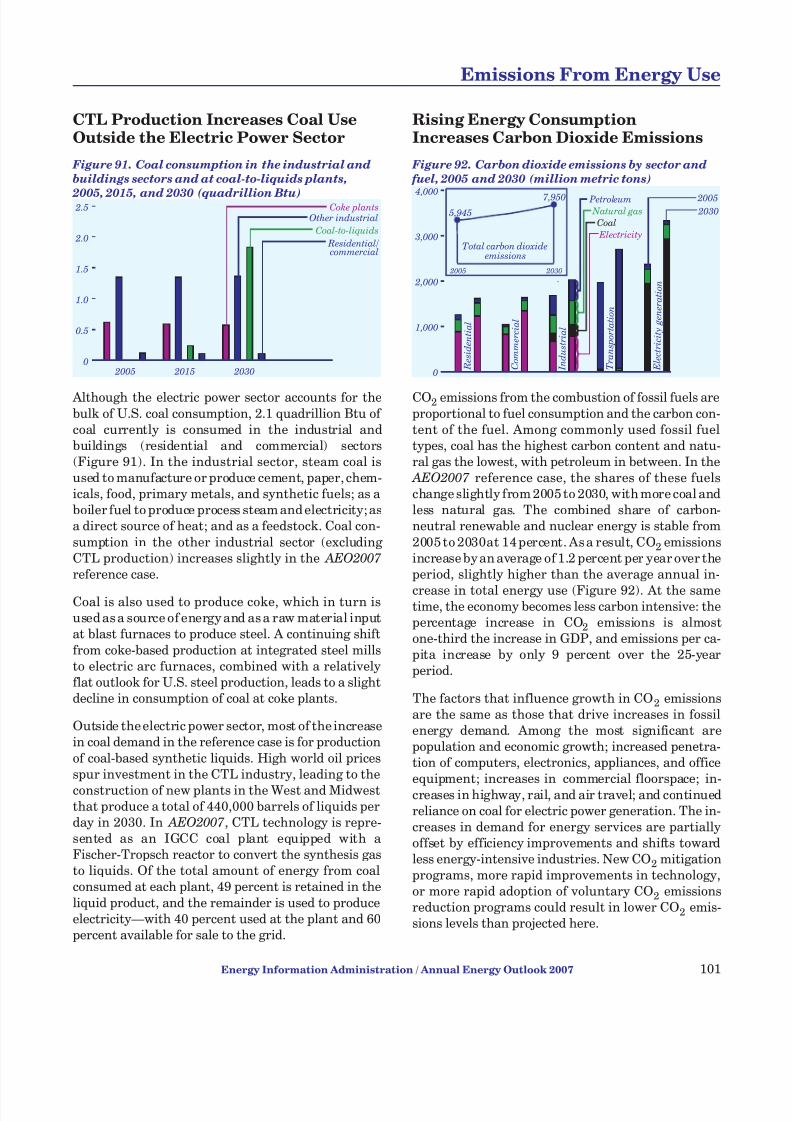
7/28/2019 2007 Annual Energy Outlook
http://slidepdf.com/reader/full/2007-annual-energy-outlook 110/243
CTL Production Increases Coal UseOutside the Electric Power Sector
Figure 91. Coal consumption in the industrial and
buildings sectors and at coal-to-liquids plants,
2005, 2015, and 2030 (quadrillion Btu)
Although the electric power sector accounts for thebulk of U.S. coal consumption, 2.1 quadrillion Btu of coal currently is consumed in the industrial andbuildings (residential and commercial) sectors(Figure 91). In the industrial sector, steam coal isused to manufacture or produce cement, paper, chem-icals, food, primary metals, and synthetic fuels; as a boiler fuel to produce process steam and electricity; asa direct source of heat; and as a feedstock. Coal con-
sumption in the other industrial sector (excluding CTL production) increases slightly in the AEO2007
reference case.
Coal is also used to produce coke, which in turn isused as a source of energy and as a raw material inputat blast furnaces to produce steel. A continuing shift
from coke-based production at integrated steel millsto electric arc furnaces, combined with a relativelyflat outlook for U.S. steel production, leads to a slightdecline in consumption of coal at coke plants.
Outside the electric power sector, most of the increasein coal demand in the reference case is for production
of coal-based synthetic liquids. High world oil pricesspur investment in the CTL industry, leading to the
construction of new plants in the West and Midwestthat produce a total of 440,000 barrels of liquids perday in 2030. In AEO2007 , CTL technology is repre-sented as an IGCC coal plant equipped with a Fischer-Tropsch reactor to convert the synthesis gasto liquids. Of the total amount of energy from coalconsumed at each plant, 49 percent is retained in the
liquid product, and the remainder is used to produceelectricity—with 40 percent used at the plant and 60percent available for sale to the grid.
Rising Energy ConsumptionIncreases Carbon Dioxide Emissions
Figure 92. Carbon dioxide emissions by sector and
fuel, 2005 and 2030 (million metric tons)
CO2 emissions from the combustion of fossil fuels areproportional to fuel consumption and the carbon con-tent of the fuel. Among commonly used fossil fueltypes, coal has the highest carbon content and natu-ral gas the lowest, with petroleum in between. In the AEO2007 reference case, the shares of these fuelschange slightly from 2005 to 2030, with more coal andless natural gas. The combined share of carbon-neutral renewable and nuclear energy is stable from
2005 to 2030at 14 percent. As a result, CO2 emissionsincrease by an average of 1.2 percent per year over theperiod, slightly higher than the average annual in-
crease in total energy use (Figure 92). At the sametime, the economy becomes less carbon intensive: thepercentage increase in CO2 emissions is almostone-third the increase in GDP, and emissions per ca-pita increase by only 9 percent over the 25-yearperiod.
The factors that influence growth in CO2 emissionsare the same as those that drive increases in fossilenergy demand. Among the most significant arepopulation and economic growth; increased penetra-tion of computers, electronics, appliances, and office
equipment; increases in commercial floorspace; in-creases in highway, rail, and air travel; and continuedreliance on coal for electric power generation. The in-creases in demand for energy services are partiallyoffset by efficiency improvements and shifts towardless energy-intensive industries. New CO2 mitigationprograms, more rapid improvements in technology,or more rapid adoption of voluntary CO2 emissionsreduction programs could result in lower CO2 emis-sions levels than projected here.
Energy Information Administration / Annual Energy Outlook 2007 101
Emissions From Energy Use
2005 2015 20300.0
0.5
1.0
1.5
2.0
2.5 Coke plants
Coal-to-liquids
Residential/ commercial
Other industrial
0
1,000
2,000
3,000
4,000
Electricity
E l e c t r i c i t y
g e n e r a
t i o n
Natural gas
Coal
Petroleum
T r a n s p o r t a
t i o n
I n d
u s t r i a
l
C o m m e r c i a
l
R e s i d e n
t i a l
2005
2030
2005 2030
Total carbon dioxide
7,950
5,945
emissions

7/28/2019 2007 Annual Energy Outlook
http://slidepdf.com/reader/full/2007-annual-energy-outlook 111/243
Emissions Projections Change WithEconomic Growth Assumptions
Figure 93. Carbon dioxide emissions, 1990-2030
(million metric tons)
Higher growth in population, labor force, and produc-tivity is assumed in the high economic growth casethan in the AEO2007 reference case, leading to high-er industrial output, higher disposable income, lowerinflation, and lower interest rates. The low economicgrowth case assumes the reverse. In the high and lowgrowth cases, GDP projections vary by about 15 per-cent and population projections by about 8 percentfrom the reference case projections for 2030.
Alternative projections for industrial output, com-mercial floorspace, housing, and transportation in the
economic growth cases influence the demand forenergy and result in variations in CO2 emissions(Figure 93). Emissions in 2030 are 10 percent lower inthe low economic growth case and 10 percent higher
in the high growth case than in the reference case.The strength of the relationship between economicgrowth and emissions varies by end-use sector. It isstrongest for the industrial sector and, to a lesser ex-tent, the transportation sector, where economic activ-ity strongly influences energy use and emissions, andwhere fuel choices are limited. It is weaker in thecommercial and residential sectors, where population
and building characteristics have large influences andvary less across the three cases.
In the electricity sector, changes in electricity salesacross the cases affect the amount of new, more effi-cient generating capacity required, reducing some-what the sensitivity of energy use to GDP. However,the choice of coal for most new baseload capacity in-
creases CO2 intensity in the high growth case whiledecreasing it in the low growth case, offsetting theeffects of changes in efficiency across the cases.
Clean Air Interstate Rule ReducesSulfur Dioxide Emissions
Figure 94. Sulfur dioxide emissions from electricity
generation, 1995-2030 (million short tons)
In March 2005, EPA promulgated the CAIR to limitformation of fine particles and ozone in nonattain-ment areas [171]. States can achieve mandated emis-sions reductions in two ways: by requiring powerplants to participate in the EPA’s national cap andtrade program or by requiring them to meet State-specific emissions milestones through measures cho-sen by the State.
The reference case projects a drop in national SO2emissions from electricity generation, from 10.2 mil-lion short tons in 2005 to 3.6 million in 2030 (Figure
94). The reduction results from both use of lower sul-fur coal and projected additions of flue gas desulfuri-zation equipment on 143 gigawatts of capacity. SO2allowance prices are projected to rise to $900 per ton
in 2015, remain between $900 and $1,100 per ton un-til 2025, and then fall to $800 per ton in 2030.
SO2 emissions projections are not greatly affected byeconomic growth assumptions. In the AEO2007 highgrowth case, with more coal-fired power plants added,the new plants are equipped for SO2 capture before
beginning operation, which is less costly than retrofit-ting existing plants. Therefore, allowance prices do
not differ by much from those in the reference case.Fuel price assumptions have a greater effect on SO2allowance prices. More CTL plants are constructed inthe high price case, and they are expected to havemore efficient SO2 capture equipment than advancedpulverized coal plants. Thus, in the last few years of the projections, SO2 allowance prices are nearly 50
percent lower in the high price case than in the refer-ence case, while the inflexible CAIR cap keeps emis-sions at nearly the same level in all cases.
102 Energy Information Administration / Annual Energy Outlook 2007
Emissions From Energy Use
1990 2000 2005 2010 2020 20300
2,000
4,000
6,000
8,000
10,000
Reference
Low growth
High growth
History Projections
11.4 11.210.2
6.6
4.5 3.9 3.7 3.6
1995 2000 2005 2010 2015 2020 2025 20300
5
10
15
20 History Projections

7/28/2019 2007 Annual Energy Outlook
http://slidepdf.com/reader/full/2007-annual-energy-outlook 112/243
Nitrogen Oxide Emissions Also Fall As CAIR Takes Effect
Figure 95. Nitrogen oxide emissions from electricity
generation, 1995-2030 (million short tons)
CAIR also mandates NOx emission reductions in 28States and the District of Columbia [172]. The re-quired reductions are intended to reduce the forma-tion of ground-level ozone, for which NOx emissionsare a major precursor. As with the CAIR-mandatedSO2 reductions, each State can determine a preferredmethod for reducing NOx emissions. Options include
joining the EPA’s cap and trade program and enforc-ing individual State regulations. Each State will be
subject to two NOx limits: a 5-month summer seasonlimit and an annual limit.
In the reference case, national NOx emissions fromthe electric power sector are projected to fall from 3.6million short tons in 2005 to 2.3 million short tons in2030 (Figure 95). Because the CAIR caps are inflexi-
ble, different assumptions in the high and low growthand high and low fuel price cases do not affect the pro-
jections for aggregate NOx emissions.
Between 2009 and 2030, after mandatory compliancebegins, NOx allowance prices are projected to rangefrom $2,400 to $3,300 per ton emitted in the reference
case, tending to rise as the emission caps tighten. By2030, selective catalytic reduction equipment is pro-
jected to be added to an additional 116 gigawatts of coal-fired generating capacity. In the high price case,with more CTL capacity built, allowances are pro-
jected to be less costly, because CTL plants emit lessNOx than the coal-fired power plants they would dis-place. In the high economic growth case, with morecoal-fired capacity in operation, allowance prices are
projected to be slightly higher than in the referencecase, even with the requirement for NOx emissioncontrols on all new plants.
Clean Air Mercury Rule ReducesMercury Emissions
Figure 96. Mercury emissions from electricity
generation, 1995-2030 (short tons)
EPA’s CAMR, also promulgated in 2005, imposes a national cap on emissions of mercury, to be imple-mented in two phases [173]. As with CAIR, States canenact their own programs or participate in the EPA cap and trade system. Although no States have madefinal decisions, more stringent regulations have beenproposed by several States in the East where manypower plants use coal with higher mercury content.
AEO2007 assumes that all States will participate inthe cap and trade program and meet the CAMR re-strictions, with no mandates for further reductions.
In the reference case, national mercury emissions areprojected to be reduced by 70 percent, from 51.3 shorttons in 2005 to 15.5 short tons in 2030 (Figure 96).Nationally, power producers are projected to retrofit
133 gigawatts of coal-fired capacity with activatedcarbon injection technology. (Mercury controls alsoare expected to help the States to meet CAIR targets,because the retrofits reduce SO2 and NOx emissionsas well.) The 2030 projection is slightly higher thanthe final EPA cap of 15 short tons, however, becauseallowances banked from earlier years could be used bysome power plants. Allowance prices are expected to
climb to a high of $68,000 per pound in 2030.Overall trends in mercury allowance prices are notgreatly affected by economic growth or fuel price as-sumptions. The AEO2007 high growth case projectsmore coal-fired generation than the reference case,causing allowance prices to rise more rapidly than inthe reference case. In the high price case, more effi-
cient CTL facilities are built, leading to a 6-percentdecrease in total annual mercury emissions in 2030relative to the reference case projection.
Energy Information Administration / Annual Energy Outlook 2007 103
Emissions From Energy Use
7.2
5.1
3.6
2.4 2.2 2.2 2.3 2.3
1995 2000 2005 2010 2015 2020 2025 20300
2
4
6
8
10 History Projections
47.850 51.3
37.2
24.6
19.216.9 15.5
1995 2000 2005 2010 2015 2020 2025 20300
10
20
30
40
50
60 History Projections
50.0

7/28/2019 2007 Annual Energy Outlook
http://slidepdf.com/reader/full/2007-annual-energy-outlook 113/243

7/28/2019 2007 Annual Energy Outlook
http://slidepdf.com/reader/full/2007-annual-energy-outlook 114/243
Comparison with Other Projections

7/28/2019 2007 Annual Energy Outlook
http://slidepdf.com/reader/full/2007-annual-energy-outlook 115/243
Only Global Insights, Inc. (GII) produces a compre-hensive energy projection with a time horizon similarto that of AEO2007 . Other organizations, however,
address one or more aspects of the energy markets.The most recent projection from GII, as well as others
that concentrate on economic growth, internationaloil prices, energy consumption, electricity, naturalgas, petroleum, and coal, are compared here with the AEO2007 projections.
Economic Growth
In the AEO2007 reference case, the projected growthin real GDP, based on 2000 chain-weighted dollars, is2.9 percent per year from 2005 to 2030. The AEO2007
projections for economic growth are based on the Au-gust short-term projection of GII, extended by EIA through 2030 and modified to reflect EIA’s view on
energy prices, demand, and production.
Projections of the average annual GDP growth ratefor the United States from 2005 through 2010 range
from 2.9 percent to 3.2 percent (Table 18). The AEO2007 reference case projects annual growth of 3.0 percent over the period, matching the projectionmade by the Social Security Administration (SSA)and GII, but it is slightly lower than the 3.2-percentreal GDP growth projected by the Office of Manage-ment and Budget (OMB), the CBO, and Energy Ven-tures Analysis, Inc. (EVA). The consensus Blue Chip
projection is for 3.0-percent average annual growthfrom 2005 to 2010. Three other organizations—Interindustry Forecasting at the University of Mary-land (INFORUM), the Bureau of Labor Statistics(BLS), and the International Energy Agency (IEA)—project somewhat lower annual growth of 2.9 percent
over the same period. The IEA projection of 2.9-percent average annual growth covers the periodfrom 2004 through 2015.
Over the period from 2010 to 2015, the uncertainty in
the projected rate of GDP growth is greater, with pro- jections ranging from 2.2 to 3.0 percent per year (ex-cluding the AEO2007 alternative cases); however, allbut one projection falls in the range of 2.7 to 3.0 per-cent—SSA with projected average growth of 2.2 per-
cent per year. The AEO2007 reference case projectionof 2.8 percent average annual economic growth from2010 to 2015 is in the middle of the range, excluding the SSA projection. The Blue Chip consensus projec-tion is 3.0 percent, and both BLS and the IEA project2.9 percent, from 2010 to 2015. Projections slightlybelow the AEO2007 reference case, at 2.7 percent, in-
clude GII, CBO, INFORUM, and EVA.
There are few public or private projections of GDPgrowth rates for the United States that extend to2030. The AEO2007 reference case projection reflectsa slowing of the GDP growth rate after 2020, consis-tent with an expected slowing of population growth.
World Oil Prices
Comparisons of the AEO2007 projections with otheroil price projections are shown in Table 19. The world
oil prices in the AEO2007 reference case generally arehigher than other world oil price projections available
for comparison. Three of the six publicly availablelong-term projections—Deutsche Bank AG (DB),Strategic Energy and Economic Research, Inc.(SEER), and EVA—anticipate that world oil priceswill decline faster than in the AEO2007 referencecase in the near term, with their projections for 2010
falling below that in the AEO2007 low price case. All
106 Energy Information Administration / Annual Energy Outlook 2007
Comparison with Other Projections
Table 18. Projections of annual average economic
growth, 2005-2030
Average annual percentage growth
Projection 2005-2010 2010-2015 2015-2020 2020-2030
AEO2006 3.2 2.9 3.1 2.8
AEO2007
Reference 3.0 2.8 3.0 2.8 Low growth 2.3 2.2 2.6 2.1
High growth 3.7 3.4 3.4 3.4
GII 3.0 2.7 2.9 2.8
OMB 3.2 NA NA NA
CBO 3.2 2.7 NA NA
Blue Chip 3.0 3.0 NA NA
INFORUM 2.9 2.7 2.7 NA
SSA 3.0 2.2 2.1 1.9
BLS 2.9 2.9 NA NA
EVA 3.2 2.7 2.3 NA
IEA 2.9 2.9 1.9 1.9
NA = not available.
Table 19. Projections of world oil prices, 2010-2030
(2005 dollars per barrel)
Projection 2010 2015 2020 2025 2030
AEO2006 (reference case) 48.72 49.24 52.24 55.72 58.69
AEO2007
Reference 57.47 49.87 52.04 56.37 59.12
Low price 49.21 33.99 34.10 34.89 35.68
High price 69.21 79.57 89.12 94.40 100.14
GII 57.11 46.54 45.06 43.21 40.25
IEA (reference) 51.50 47.80 50.20 52.60 55.00
EEA 56.94 49.80 47.42 45.16 NA
DB 39.66 40.11 39.73 39.95 40.16
SEER 44.21 45.27 45.87 46.23 46.60
EVA 42.28 42.35 45.76 49.45 NA

7/28/2019 2007 Annual Energy Outlook
http://slidepdf.com/reader/full/2007-annual-energy-outlook 116/243
the projections—except for the price projection fromEVA, which was not available for comparison in last
year’s outlook—have raised their price expectations
for 2010 and in the longer term relative to last year’sreleases.
The world oil price measures are, by and large, com-parable across projections. For AEO2007 , EIA reportsthe price of imported low-sulfur, light crude oil, ap-proximately the same as the WTI prices that are
widely cited as a proxy for world oil prices in the tradepress. The only series that does not report projectionsin WTI terms is the IEA’s World Energy Outlook
2006, where prices are expressed as the IEA crude oilimport price.
Recent variability in crude oil prices demonstrates
the uncertainty inherent in the projections. The AEO2007 reference case and DB define the range of projected prices among the comparative seriesthroughout the projection period. The range among the projections is $18 per barrel in 2010 (from a lowprice of $39.66 per barrel to a high of $57.47 per bar-rel), declining to $10 per barrel in 2015 and then wid-ening to $19 per barrel in 2030 (from a low of $40.16per barrel to a high of $59.12 per barrel).
Excluding the AEO2007 high and low price cases,there are four distinct views proffered by the compar-ative series beginning in 2010: (1) prices moderate by
2015 before beginning a steady increase; (2) prices donot moderate over the mid-term but increase toward
the end of the projection; (3) prices decline through-out the projection; and (4) prices remain relativelyflat throughout. In the AEO2007 reference case,prices decline from about $57 per barrel in 2010 to$50 per barrel in 2015 and rise steadily to $59 per bar-rel in 2030 (all prices expressed in real 2005 dollars).IEA projects a similar trend. In the EVA projection,prices remain flat until after 2015, then begin to rise.
Although GII and Energy and Environmental Analy-
sis, Inc. (EEA) anticipate a (rather sharper) decline in
prices over the 2010 to 2015 period compared to the AEO2007 reference case, both expect the decline tocontinue, albeit slowly, through the end of their re-spective projection periods. Finally, DB and SEER ex-pect oil prices to remain relatively flat or increaseslightly from 2010 to 2030.
Total Energy Consumption
The AEO2007 reference case projects higher growthin end-use sector consumption of petroleum, natural
gas, and coal than occurred from 1980 to 2005 but
lower growth in electricity consumption (Table 20).Much of the projected growth in petroleum consump-tion is driven by increased demand in the transporta-
tion sector, with continued growth in personal traveland freight transport projected to result from demo-
graphic trends and economic expansion. Natural gasconsumption is expected to increase in the residen-tial, commercial, and industrial sectors, despite rela-tively high prices. Natural gas is cleaner than otherfuels, does not require on-site storage, and has tendedto be priced competitively with oil for heating. Coalconsumption as a boiler fuel in the commercial and in-
dustrial sectors is expected to decline slightly, withpotential use in new boilers limited by environmentalrestrictions; however, the projections for industrialcoal include its use in CTL plants, a technology that isexpected to become competitive at the level of oil
prices assumed in the AEO2007 reference case.
While strong growth in electricity use is projected tocontinue in the AEO2007 reference case, the paceslows from historical rates. Some rapidly growing ap-plications, such as air conditioning and computers,slow as penetration approaches saturation levels.Electrical efficiency also continues to improve, due inlarge part to efficiency standards, and the impactstend to accumulate with the gradual turnover of ap-
pliance stocks.
The AEO2007 reference case generally includes
greater growth in primary energy consumptionthrough 2030 than is shown in the outlook fromGII. GII projects little growth in end-use natural gasconsumption, whereas the AEO2007 reference case
projects continued growth in the industrial andbuildings sectors. Some of the difference can be at-tributed to the higher natural gas price assumptionsin the GII projection. End-use natural gas prices in
Energy Information Administration / Annual Energy Outlook 2007 107
Comparison with Other Projections
Table 20. Projections of average annual growth
rates for energy consumption, 2005-2030 (percent)
Energy use
History
1980-2005
Projections
AEO2007 GII Petroleum* 0.9 1.0 0.9
Natural gas* 0.0 0.9 0.1
Coal* -1.7 1.4 -0.2
Electricity 2.2 1.4 1.3
Delivered energy 0.7 1.1 0.8
Electricity losses 1.9 1.0 0.7
Primary energy 1.0 1.1 0.7
*Excludes consumption by electricity generators in the electric power sector; includes consumption for end-use combined heat and power generation.

7/28/2019 2007 Annual Energy Outlook
http://slidepdf.com/reader/full/2007-annual-energy-outlook 117/243
the AEO2007 reference case decline rapidly from2006 to 2013 before resuming a slow upward trend. Incontrast, GII projects a more moderate decline in nat-
ural gas prices from 2005 to 2015, with little furtherchange by 2025. GII projects an industrial natural gas
price of $7.91 per thousand cubic feet in 2025, com-pared with $6.40 per thousand cubic feet in the AEO2007 reference case (2005 dollars). GII’s pro- jected growth rates for petroleum and electricity con-sumption are similar to those in the AEO2007
reference case. Differences between the AEO2007 ref-erence case and the GII projections for end-use coal
consumption result from a projected increase in coaluse for CTL in the AEO2007 reference case.
Electricity
The AEO2007 projections of retail electricity prices
are based on average costs for electricity. The projec-tions include supply regions that still are regulated,regions that are competitive and where marginalrather than average prices are assumed, and regionswith a mix of regulated and competitive marketswhere average and marginal prices are weighted by
the amount of load that serves regulated and competi-tive markets. As of 2005, 4 of the 13 electricity marketregions had fully competitive retail markets in opera-tion, 7 regions had mixed competitive and regulatedretail markets, and 2 regions had fully regulated mar-kets. The AEO2007 cases assume that no additional
retail markets will be restructured and that partialrestructuring (in wholesale markets) will lead to in-
creased competition in the electric power industry.Competition is assumed to lower operating and main-tenance costs and to cause the retirement of uneco-nomical generating units. The AEO2007 electricityprojections assume continuation of current laws andregulations. Other projections may reflect explicit as-sessments of the nature and likelihood of policy devel-opments over the next 25 years.
Comparisons of the AEO2007 projections and those
from other organizations are shown in Table 21. Theprojections for electricity sales in 2015 range from a low of 4,133 billion kilowatthours in the AEO2007
low economic growth case to a high of 4,433 billionkilowatthours in the EVA projection. EVA projectshigher sales in the commercial and residential sec-tors, with somewhat less growth in industrial sales,than are projected by the AEO2007 reference case,GII, and EEA. The projections for total electricity
sales in 2030 range from 4,682 billion kilowatthours( AEO2007 low economic growth case) to 5,654 billion
kilowatthours ( AEO2007 high economic growthcase). The annual rate of demand growth ranges from1.0 percent ( AEO2007 low economic growth case) to
1.8 percent ( AEO2007 high economic growth case).GII projects lower growth in the commercial sector
and higher growth in the industrial and, to a lesserextent, residential sectors in 2030 than is projected inthe AEO2007 reference case.
The AEO2007 reference case shows a decline in realelectricity prices early in the projection period andthen rising prices at the end of the period because of increases in the cost of fuels used for generation and
increases in capital expenditures for construction of new capacity. The rising fossil fuel prices and in-creased capital outlays in the AEO2007 reference caselead to an increase in average electricity prices, from
7.7 cents per kilowatthour in 2015 to 8.1 cents perkilowatthour in 2030. GII projects increases in pricesinitially and then a slight decline at the end of theperiod.
Projections of total electricity generation in 2015 are
similar for the AEO2007 reference case, EVA, andEEA. In contrast, the projection by GII is lower thanthe others because of lower projected growth in elec-tricity sales. The GII projection of total electricitygeneration in 2015 is similar to that in the AEO2007
low economic growth case. Although GII projects a lower level of total electricity generation in 2030 than
is projected in the AEO2007 reference and high eco-nomic growth cases, its projection for renewable gen-
eration in 2030 is considerably higher than the AEO2007 reference case projection.
The need for new generating capacity is driven bygrowth in electricity sales and the need to replace ex-isting units that are no longer economical to operate.Consistent with its projection of higher growth inelectricity sales, EVA projects greater growth in re-quirements for new fossil-fuel-fired generating plantsas well as nuclear plants in 2015 compared with the
AEO2007 reference case and GII. Except for nuclearplants, the EVA projections for generating capacityare similar to EEA’s projections for 2015. As notedabove, the GII projections for renewable capacity in2030 are higher than those in the AEO2007 referenceand high and low economic growth cases. The projec-tions for nuclear capacity additions from 2005 to2030 as a result of the incentives in EPACT2005range from 28 gigawatts in the AEO2007 high eco-
nomic growth case to 6 gigawatts in the AEO2007 loweconomic growth case. The AEO2007 cases assume
108 Energy Information Administration / Annual Energy Outlook 2007
Comparison with Other Projections

7/28/2019 2007 Annual Energy Outlook
http://slidepdf.com/reader/full/2007-annual-energy-outlook 118/243
Energy Information Administration / Annual Energy Outlook 2007 109
Comparison with Other Projections
Table 21. Comparison of electricity projections, 2015 and 2030 (billion kilowatthours, except where noted)
Projection 2005
AEO2007 Other projections
Reference Low
economic growth
High economic
growthGII EVA EEA
2015
Average end-use price(2005 cents per kilowatthour) 8.1 7.7 7.5 7.9 8.6 NA NA
Residential 9.4 8.9 8.7 9.1 10.0 9.7 NA
Commercial 8.6 8.0 7.7 8.2 9.2 8.7 NA
Industrial 5.7 5.6 5.4 5.9 5.8 5.6 NA
Total generation plus imports 4,063 4,729 4,597 4,865 4,610 4,720 4,766
Coal 2,015 2,295 2,235 2,353 2,244 2,336 NA
Oil 122 103 100 105 92 NA NA
Natural gas a 756 1,023 959 1,068 934 982 NA
Nuclear 780 812 809 837 829 860 NA
Hydroelectric/other b 365 487 485 493 492 523 NA
Net imports 25 8 8 10 20 20 NA
Electricity sales 3,660 4,251 4,133 4,370 4,186 4,433 4,302
Residential 1,365 1,591 1,560 1,622 1,592 1,665 1,597 Commercial/other c 1,274 1,557 1,532 1,583 1,485 1,709 1,507
Industrial 1,021 1,103 1,041 1,165 1,110 1,059 1,198
Capability, including CHP (gigawatts) d 988 997 981 1,018 1,011 1,045 1,035
Coal 315 329 322 336 333 351 346
Oil and natural gas 448 430 422 440 429 453 457
Nuclear 100 102 102 106 104 108 102
Hydroelectric/other 125 136 135 136 146 132 130
2030
Average end-use price(2005 cents per kilowatthour) 8.1 8.1 7.8 8.4 8.5 NA NA
Residential 9.4 9.1 8.8 9.6 9.9 NA NA
Commercial 8.6 8.3 7.9 8.7 9.1 NA NA
Industrial 5.7 5.9 5.6 6.3 5.6 NA NA
Total generation plus imports 4,065 5,810 5,255 6,375 5,586 NA NACoal 2,015 3,330 2,871 3,672 2,999 NA NA
Oil 122 107 104 112 76 NA NA
Natural gas a 756 942 924 1,010 952 NA NA
Nuclear 780 896 845 1,010 826 NA NA
Hydroelectric/other b 365 522 499 555 719 NA NA
Net imports 25 13 12 15 15 NA NA
Electricity sales 3,660 5,168 4,682 5,654 5,071 NA NA
Residential 1,365 1,896 1,773 2,016 1,921 NA NA
Commercial/other c 1,274 2,073 1,907 2,234 1,872 NA NA
Industrial 1,021 1,199 1,003 1,403 1,278 NA NA
Capability, including CHP (gigawatts) d 988 1,220 1,112 1,331 1,157 NA NA
Coal 315 465 403 511 443 NA NA
Oil and natural gas 448 500 464 544 404 NA NA
Nuclear 100 113 106 127 109 NA NA
Hydroelectric/other 125 142 138 149 202 NA NA
a Includes supplemental gaseous fuels. For EVA, represents total oil and natural gas. b“Other” includes conventional hydroelectric,pumped storage, geothermal, wood, wood waste, municipal waste, other biomass, solar and wind power, batteries, chemicals, hydrogen,pitch, purchased steam, sulfur, petroleum coke, and miscellaneous technologies. c“Other” includes sales of electricity to government,railways, and street lighting authorities. dEIA capacity is net summer capability, including combined heat and power plants. GII capacity isnameplate, excluding cogeneration plants.
CHP = combined heat and power. NA = not available.Sources: 2005 and AEO2007: AEO2007 National Energy Modeling System, runs AEO2007.D112106A (reference case), LM2007.
D112106A (low economic growth case), and HM2007.D112106A (high economic growth case). GII: Global Insight, Inc., 2006 U.S. EnergyOutlook (November 2006). EVA: Energy Ventures Analysis, Inc., FUELCAST: Long-Term Outlook (August 2006). EEA: Energy andEnvironmental Analysis, Inc., EEA’s Compass Service Base Case (October 2006).

7/28/2019 2007 Annual Energy Outlook
http://slidepdf.com/reader/full/2007-annual-energy-outlook 119/243
that 2.6 gigawatts of nuclear capacity will be retiredby 2030 because their operating licenses will haveexpired.
Environmental regulations have an important influ-
ence on the technology choices made for electricitygeneration. EVA assumes that legislation similar tothe Clear Skies Act (including new restrictions onSO2, NOx, and mercury emissions) will be in effect by2010. EVA also includes a tax of $6 per ton on CO2emissions beginning in 2013. The combination of stronger environmental restrictions, a tax on CO2emissions, and aggregate State-level RPS program re-quirements leads to greater growth in nonhydro-electric renewable generation in the EVA projectionthan in the other projections in 2015. The AEO2007
cases reflect EPA’s recently enacted CAIR and CAMR
regulations. Because AEO2007 generally includesonly current laws and regulations, it does not assume
any policies to address CO2 emissions. As notedabove, restrictions on CO2 emissions could change themix of technologies used to generate electricity.
Natural Gas
In the AEO2007 reference case, natural gas consump-tion is projected to grow steadily through 2020 andthen level off as higher projected natural gas pricescause natural gas to lose market share to coal for elec-tricity generation. With the exception of GII, this is a
major difference between the AEO2007 reference andhigh price cases and the other projections (Table 22),
which show natural gas consumption generally in-creasing throughout the projection period, both over-all and for electricity generation. The lowest projectedoverall growth is in the GII projection, with 2030 con-sumption that is 2.4 trillion cubic feet less than in the AEO2007 reference case. The DB, SEER, and Altosprojections expect natural gas consumption in 2030 toexceed the AEO2007 reference case projection by 1.1,4.1, and 4.8 trillion cubic feet, respectively; the two
latter projections even exceed the AEO2007 low price
case projection. Although GII projects less total natu-ral gas consumption than does the AEO2007 refer-ence case, the GII projection for consumption byelectricity generators exceeds that in the AEO2007
reference case, further highlighting a fundamentaldifference between the AEO2007 reference case andthe other projections.
Natural gas consumption by electricity generatorsgrows from 2005 to 2015 in all the projections. Withthe exception of the AEO2007 reference and high
price cases, the projected growth continues through2025. DB is the only projection with less growth innatural gas consumption by electricity generators
than the AEO2007 reference case from 2005 to 2015.Natural gas consumption in the DB projection in 2015
is 6 percent below the AEO2007 reference case value,and the other projections are between 2 percent (GII)and 32 percent (Altos) above the AEO2007 referencecase. In 2025, natural gas consumption by electricitygenerators in all the other projections exceeds that inthe AEO2007 reference case by 6 percent (DB) to 69percent (Altos). In 2030, consumption in the other
projections is 20 percent (DB) to 109 percent (Altos)higher than in the AEO2007 reference case. Only theGII and DB projections for natural gas consumptionby electricity generators are consistently lower thanthose in the AEO2007 low price case.
All the projections show steady growth in natural gas
consumption in the combined residential and com-mercial sectors, with the exception of GII, which ex-pects a slight decline in consumption from 2025 to2030. The AEO2007 reference case shows higher in-dustrial natural gas consumption than all the otherprojections over the entire 2005-2030 period. Withthe exception of GII and EEA, all the other organiza-tions project growth in industrial natural gas con-
sumption from 2005 to 2015 and through the end of the projection period. Growth in residential, commer-cial, and industrial natural gas consumption in the AEO2007 reference case is offset, however, by thedecline in natural gas consumption by electricitygenerators.
Domestic natural gas production is projected to de-cline in the GII, EVA, and Altos projections over thenext decade; in all the other projections it increases
over the same period. GII and EVA expect the declineto be reversed in 2025, with production slightly ex-ceeding 2005 production levels. DB and Altos aremore pessimistic, projecting that natural gas produc-tion will have declined by about 10 percent in 2025
relative to 2005 levels. Altos expects domestic naturalgas production in 2030 to be 21 percent below 2005levels. The AEO2007 high price case shows domesticnatural gas production of 20.9 trillion cubic feet in
2030, one of the more optimistic projections. It is ex-ceeded only by the SEER projection of 21.2 trillion cu-bic feet in 2030.
With the exception of the AEO2007 high price case,net imports increase significantly from 2005 to 2030in all the projections, with increases ranging from
110 Energy Information Administration / Annual Energy Outlook 2007
Comparison with Other Projections

7/28/2019 2007 Annual Energy Outlook
http://slidepdf.com/reader/full/2007-annual-energy-outlook 120/243
approximately 50 percent in the AEO2007 referencecase and GII projections to 255 percent in the Altosprojection. The increase is expected to come from
LNG. With the exception of the DB projection and the AEO2007 high price case, all the projections show
higher LNG imports than the AEO2007 referencecase in 2015. Net LNG imports in 2015 in the Altosprojection, at 6.8 trillion cubic feet, are significantlyhigher than those in the other projections; and Altosremains the most optimistic projection in 2030, at12.0 trillion cubic feet of net LNG imports. Net LNGimports are 4.5 trillion cubic feet in 2030 in the
AEO2007 reference case, by far the lowest level of
imports of any of the projections, with DB and Altosprojecting more than double that level. LNG importsin the AEO2007 high price case are even lower, at 2.3
trillion cubic feet in 2030. The AEO2007 referencecase also projects the lowest percentage of consump-
tion accounted for by LNG imports. LNG imports ac-count for slightly under 17 percent of total naturalgas consumption in 2025 in the AEO2007 referencecase—about the same as in the EEA projection—whereas the other organizations expect LNG importsto account for between 21 and 40 percent of consumption.
Energy Information Administration / Annual Energy Outlook 2007 111
Comparison with Other Projections
Table 22. Comparison of natural gas projections, 2015, 2025, and 2030 (trillion cubic feet, except where noted)
Projection 2005
AEO2007 Other projections
Refer- ence
Low price
High price
GII a EVA EEAb DB SEER Altos
2015
Dry gas production c 18.23 19.60 19.82 18.77 17.45 17.93 20.42 19.53 18.87 18.19
Net imports 3.57 5.62 6.46 4.81 5.73 7.95 5.40 4.90 6.50 8.06
Pipeline 3.01 2.63 2.48 2.52 NA 3.73 2.26 2.60 2.80 1.22
LNG 0.57 2.99 3.98 2.29 NA 4.22 3.13 2.29 3.70 6.84
Consumption 21.98 25.32 26.40 23.71 23.38 25.67 26.00 24.20 25.37 25.87 d
Residential 4.84 5.19 5.29 5.11 4.99 5.14 5.49 5.30 5.12 5.41
Commercial 3.05 3.53 3.65 3.42 3.05 3.11 3.40 3.42 3.18 3.54
Industrial e 6.64 7.67 7.71 7.44 6.48 6.95 6.39 7.19 6.99 7.53 f
Electricity generators g 5.78 7.11 7.89 5.99 7.26 8.50 8.53 6.71 8.10 9.39
Other h 1.66 1.83 1.86 1.75 1.61 1.97 2.18 1.59 1.99 NA
Lower 48 wellhead price (2005 dollars per thousand cubic feet) i
7.51 4.99 4.01 5.83 6.10 5.55 6.51 6.07 5.12 5.60
End-use prices (2005 dollars per thousand cubic feet)
Residential 12.80 10.55 9.48 11.48 11.28 NA 10.95 NA 10.59 NA
Commercial 11.54 8.73 7.68 9.64 10.05 NA 9.98 NA 8.83 NA
Industrial j 8.41 5.82 4.80 6.70 7.87 NA 7.95 NA 6.45 NA
Electricity generators 8.42 5.66 4.74 6.40 6.68 NA 7.54 NA 6.11 NA
2025
Dry gas production c 18.23 20.59 20.44 20.73 18.26 18.82 22.61 16.67 20.91 16.41
Net imports 3.57 5.58 8.70 3.32 5.23 9.93 6.28 9.54 7.80 12.59
Pipeline 3.01 1.20 1.58 1.03 NA 2.11 1.24 1.25 1.80 1.10
LNG 0.57 4.38 7.11 2.29 NA 7.82 5.04 8.29 6.00 11.49
Consumption 21.98 26.30 29.27 24.13 23.69 28.53 29.03 26.18 28.71 29.01 d
Residential 4.84 5.29 5.38 5.21 4.97 5.18 5.86 5.85 5.64 6.03
Commercial 3.05 3.98 4.06 3.82 3.07 3.42 3.55 3.87 3.45 4.14 Industrial e 6.64 8.42 8.09 7.94 6.53 7.95 7.10 7.94 7.66 7.69 f
Electricity generators g 5.78 6.59 9.71 4.82 7.45 9.74 10.25 6.98 9.78 11.15
Other h 1.66 2.02 2.03 1.99 1.67 2.24 2.27 1.54 2.18 NA
Lower 48 wellhead price (2005 dollars per thousand cubic feet) i
7.51 5.62 4.75 6.70 6.21 6.06 6.83 5.71 5.61 6.96
End-use prices (2005 dollars per thousand cubic feet)
Residential 12.80 11.30 10.32 12.43 11.21 NA 10.95 NA 11.19 NA
Commercial 11.54 9.23 8.29 10.34 10.02 NA 10.08 NA 9.51 NA
Industrial j 8.41 6.40 5.52 7.51 7.91 NA 8.22 NA 7.12 NA
Electricity generators 8.42 6.22 5.56 7.18 6.78 NA 7.85 NA 6.78 NA
NA = not available. See notes and sources at end of table.

7/28/2019 2007 Annual Energy Outlook
http://slidepdf.com/reader/full/2007-annual-energy-outlook 121/243
For the most part, all the projections expect naturalgas wellhead prices to decline significantly from the2005 level of $7.51 per thousand cubic feet. The
AEO2007 low price case shows the lowest projectionfor natural gas wellhead prices in 2015 [174], followed
by the AEO2007 reference case. Natural gas wellheadprices in the AEO2007 reference and low price casesin 2025 are at or below the levels in all the other pro-
jections. Among the other organizations, only DBprojects a natural gas wellhead price below that inthe AEO2007 reference case for 2030, and only Altosprojects a price that exceeds the 2005 price. In the GII
and SEER projections, natural gas wellhead prices in2030 exceed the AEO2007 reference case projectionby less than 2 percent, and the Altos price projectionfor 2030 exceeds the AEO2007 reference case projec-tion by 26 percent.
Delivered natural gas price margins [175 ] to electric-ity generators are consistently the lowest in the
AEO2007 high price case and GII projections. Both
are notably lower than the historically high marginsin 2005. The margins in the SEER projection exceed
those in the AEO2007 reference case in all years by upto 120 percent. While the industrial sector margins inthe other projections exceed those in the AEO2007
reference case in all years by as much as 120 percent[176], the disparity is largely attributable to defini-tional differences, which can be seen by comparing the 2005 values provided with the other projections.
All projections show a decline in industrial marginsacross the projection period relative to their 2005 val-ues. SEER shows the greatest percentage declinefrom 2005 to 2025, at 17 percent; EEA shows thesmallest decline at 5 percent; and the rest show
112 Energy Information Administration / Annual Energy Outlook 2007
Comparison with Other Projections
Table 22. Comparison of natural gas projections, 2015, 2025, and 2030 (continued)
(trillion cubic feet, except where noted)
Projection 2005
AEO2007 Other projections
Refer- ence
Low price
High price
GII a
EVA EEAb
DB SEER Altos
2030
Dry gas production c 18.23 20.53 20.64 20.90 18.27 NA NA 16.32 21.17 14.33
Net imports 3.57 5.45 8.85 3.17 5.25 NA NA 10.72 9.08 12.67
Pipeline 3.01 0.92 1.31 0.84 NA NA NA 1.25 1.44 0.70
LNG 0.57 4.53 7.54 2.33 NA NA NA 9.47 7.64 11.97
Consumption 21.98 26.12 29.74 24.09 23.74 NA NA 27.20 30.26 30.95 d
Residential 4.84 5.31 5.40 5.20 4.92 NA NA 6.15 5.92 6.34
Commercial 3.05 4.24 4.32 4.01 3.07 NA NA 4.06 3.56 4.44
Industrial e 6.64 8.65 8.34 8.18 6.79 NA NA 8.34 7.82 7.78 f
Electricity generators g 5.78 5.92 9.64 4.37 7.27 NA NA 7.12 10.74 12.39
Other h 1.66 2.01 2.05 2.00 1.68 NA NA 1.52 2.22 NA
Lower 48 wellhead price (2005 dollars per thousand cubic feet) i
7.51 5.98 5.06 7.63 6.08 NA NA 5.45 6.07 7.55
End-use prices (2005 dollars per thousand cubic feet)
Residential 12.80 11.77 10.71 13.52 10.98 NA NA NA 11.58 NA
Commercial 11.54 9.58 8.58 11.32 9.81 NA NA NA 9.96 NA
Industrial j 8.41 6.76 5.82 8.46 7.74 NA NA NA 7.58 NA
Electricity generators 8.42 6.51 5.88 8.02 6.65 NA NA NA 7.25 NA
NA = not available.a Previously DRI-WEFA. Conversion factors: 1,000 cubic feet = 1.027 million Btu for production, 1.028 million Btu for end-useconsumption, 1.019 million Btu for electric power. bThe EEA projection shows a cyclical price trend; projected values for isolated years maybe misleading. cDoes not include supplemental fuels. dExcludes consumption for transportation and pipeline fuels. eIncludes consumptionfor industrial CHP plants and a small number of electricity-only plants; excludes consumption by nonutility generators. f Includes lease andplant fuel. g Includes consumption of energy by electricity-only and CHP plants whose primary business is to sell electricity, or electricityand heat, to the public. Includes electric utilities, small power producers, and exempt wholesale generators. hIncludes lease, plant, andpipeline fuel andfuel consumed in natural gasvehicles. i2005wellhead natural gasprices for EEA, EVA, and DB are $7.77, $8.84, and $8.36,respectively. jThe 2005 industrial natural gas prices in other projections are nearly a dollar higher than EIA’s.
Sources: 2005 and AEO2007 : AEO2007 National Energy Modeling System, runs AEO2007.D112106A (reference case), LP2007.D112106A (low price case), HP2007.D112106A (high price case). GII: Global Insight, Inc., 2006 U.S. Energy Outlook (November 2006).EVA: Energy Ventures Analysis, Inc., FUELCAST: Long-Term Outlook (August 2006). EEA: Energy and Environmental Analysis, Inc., EEA’s Compass Service Base Case (October 2006). DB: Deutsche Bank AG, e-mail from Adam Sieminski on November 27, 2006. SEER:Strategic Energy and Economic Research, Inc., Natural Gas Outlook (April 2006). Altos: Altos Partners North American Regional GasModel (NARG) Long-Term Base Case (November 2006).

7/28/2019 2007 Annual Energy Outlook
http://slidepdf.com/reader/full/2007-annual-energy-outlook 122/243
declines of around 13 percent. Residential and com-mercial sector margins are, on average, about $5.40and $3.70, respectively, with residential sector mar-
gins in the AEO2007 reference case generally higherthan those in the projections from other organiza-
tions, and commercial sector margins generallylower.
Petroleum
With significantly lower crude oil prices, the DB pro- jections of U.S. petroleum demand in 2015 and 2030
are only 2 percent higher than those in the AEO2007
reference case (Table 23). In the IEA reference case,total petroleum consumption in 2015 is within 1 per-cent of the total petroleum consumption in the AEO2007 reference case; but in 2030, IEA’s totalpetroleum demand projection is 7 percent lower than
in the AEO2007 reference case. Although the crudeoil price is almost $19 per barrel lower than that in
the AEO2007 reference case in 2030, total petroleumdemand in the GII projection is lower than in the AEO2007 reference case throughout the projectionperiod. The GII projection shows the lowest level of petroleum demand among the projections reviewed,lower than the AEO2007 high price case projection.The AEO2007 low price case shows the highest levelsof total petroleum demand in 2015 and 2030 among all the projections. The AEO2007 high price case also
shows higher petroleum demand than the GII projec-
tion in 2030, with projected crude oil prices that arealmost $60 per barrel higher. The extent to which theprojections from other organizations reviewed aboveand summarized in Table 24 incorporate expectationsof changes in vehicle efficiency standards or other pol-icy actions that could influence petroleum demand isnot clear.
The projection of domestic crude oil production in the AEO2007 reference case differs significantly from theother projections; rising from 5.2 million barrels in2005 to a peak of 5.9 million barrels per day in 2017
and then declining to 5.4 million barrels per day in2030. With the exception of the IEA reference case,domestic crude oil production in the other projectionsdeclines throughout the projection period to levelsmore than a million barrels per day lower than in the AEO2007 reference case. Domestic crude oil produc-tion falls to 3.4 million barrels per day in 2025 in theEVA projection and 3.5 million barrels per day in
2030 in the DB projection. In the IEA projection, do-
mestic crude oil production increases until 2010, thendeclines to 4.0 million barrels per day in 2030.
The higher crude oil prices in the AEO2007 referencecase alone do not fully explain the differences in theprojections for domestic crude oil production. For ex-
ample, crude oil prices in the IEA projection areslightly higher than in the AEO2007 reference case
from 2012 through 2030, but domestic crude oil pro-duction in 2030 is more than 1 million barrels per daybelow domestic crude oil production in the AEO2007
reference case. The AEO2007 low price case, withcrude oil prices in the mid-$30 per barrel range from2015 through 2030, shows the same pattern of domes-tic crude oil production as the AEO2007 reference
case. Production rises from current levels, peaks in2015, and then gradually declines but still ends upslightly higher in 2030 than the current level of pro-duction. The AEO2007 high price case projects in-creasing domestic crude oil production, peaking in
2030 at more than 6.0 million barrels per day.
The projections also differ on domestic NGL produc-tion. In the AEO2007 reference case, NGL productionincreases from current levels to a peak of 1.8 millionbarrels per day in 2017 before falling back to 1.7 mil-lion barrels per day in 2030, about equal to the 2005level. NGL production is 17 percent lower in 2015 in
the DB projection and 37 percent lower in 2030 thanin the AEO2007 reference case. The GII projection ismore bullish, with 2030 NGL production slightlyhigher than in the AEO2007 reference case.
The differences in domestic crude oil production leadto very different conclusions about U.S. dependenceon imported petroleum. In the AEO2007 reference
case, the import share of product supplied decreasesfrom 60 percent in 2005 to below 55 percent in 2009and then slowly rises back to 61 percent in 2030. Theshare of imported petroleum increases from 2005 lev-els in the DB and GII projections throughout the pro-
jection period, to 77 percent in 2030 in the DBprojection and 75 percent in 2030 in the GII projec-tion. Despite higher petroleum demand in the
AEO2007 low price case, the projected import share
rises to only 67 percent in 2030. In the AEO2007 highprice case, the import share is projected to decline to49 percent in 2030, well below 2005 levels.
Coal
The coal consumption, production, and price projec-tions vary considerably, reflecting uncertainty aboutenvironmental regulations and economic growth,
among many factors (Table 24). The coal projectionsfrom the AEO2007 cases reflect existing environmen-tal regulations, including CAAA90, CAIR, and CAMR,
Energy Information Administration / Annual Energy Outlook 2007 113
Comparison with Other Projections

7/28/2019 2007 Annual Energy Outlook
http://slidepdf.com/reader/full/2007-annual-energy-outlook 123/243
which restrict SO2, NOx, and mercury emissions be-ginning in 2010. The EVA projection incorporatessimilar regulations and also includes a carbon tax of
$6 per metric ton CO2 equivalent beginning in 2013.In addition to differences in environmental assump-
tions, the AEO2007 , EVA, and GII projections reflectdifferent assumptions about the outlook for economic
growth rates, the natural gas prices, and world oilprices.
All the projections show increases in total coal con-sumption over their projection periods. Despite early
similarities between the projections, total coal con-sumption in the AEO2007 reference case after 2015
114 Energy Information Administration / Annual Energy Outlook 2007
Comparison with Other Projections
Table 23. Comparison of petroleum projections, 2015, 2025, and 2030
(million barrels per day, except where noted)
Projection 2005 AEO2007 Other projections
Reference Low price High price GII EVA DB IEA
2015
Crude oil and NGL production 6.90 7.73 8.02 7.41 6.47 6.09 6.28 NACrude oil 5.18 5.91 6.18 5.67 4.80 4.45 4.78 5.00 Natural gas liquids 1.72 1.82 1.84 1.74 1.67 1.64 1.50 NA
Total net imports 12.57 12.52 13.29 11.79 13.75 NA 15.37 NACrude oil 10.09 10.49 10.62 10.18 NA NA NA NA Petroleum products 2.48 2.03 2.67 1.61 NA NA NA NA
Petroleum demand 20.75 22.86 23.61 21.87 20.22 NA 23.26 23.10 Motor gasoline 9.16 10.18 10.45 9.53 NA NA 10.32 NA Jet fuel 1.68 2.10 2.12 2.08 NA NA 1.87 NA Distillate fuel 4.12 4.86 5.04 4.72 NA NA 4.81 NA Residual fuel 0.92 0.82 1.03 0.73 NA NA 0.78 NAOther 4.87 4.89 4.96 4.81 NA NA 5.48 NA
Import share of product supplied(percent) 60 55 56 54 68 NA 66 NA
2025
Crude oil and NGL production 6.90 7.30 7.34 7.68 6.02 4.95 5.11 NACrude oil 5.18 5.58 5.60 5.97 4.27 3.35 3.91 NA Natural gas liquids 1.72 1.72 1.74 1.70 1.75 1.60 1.20 NA
Total net imports 12.57 14.87 16.98 11.70 17.03 NA 19.31 NACrude oil 10.09 12.20 13.27 10.19 NA NA NA NA
Petroleum products 2.48 2.67 3.71 1.51 NA NA NA NA Petroleum demand 20.75 25.34 26.77 23.50 23.05 NA 26.15 NA
Motor gasoline 9.16 11.71 12.26 10.14 NA NA 11.57 NA Jet fuel 1.68 2.22 2.24 2.12 NA NA 2.14 NA Distillate fuel 4.12 5.48 5.88 5.35 NA NA 5.47 NA Residual fuel 0.92 0.82 1.11 0.75 NA NA 0.83 NAOther 4.87 5.11 5.29 5.14 NA NA 6.15 NA
Import share of product supplied(percent) 60 59 64 50 74 NA 74 NA
2030
Crude oil and NGL production 6.90 7.10 6.98 7.75 5.79 NA 4.62 NACrude oil 5.18 5.39 5.25 6.04 4.04 NA 3.53 4.00 Natural gas liquids 1.72 1.72 1.73 1.71 1.75 NA 1.08 NA
Total net imports 12.57 16.37 19.31 12.04 17.03 NA 21.13 NACrude oil 10.09 13.09 14.35 10.59 NA NA NA NA
Petroleum products 2.48 3.28 4.95 1.45 NA NA NA NA Petroleum demand 20.75 26.95 28.84 24.58 22.82 NA 27.54 25.00 Motor gasoline 9.16 12.53 13.23 10.47 NA NA 12.16 NA Jet fuel 1.68 2.27 2.29 2.06 NA NA 2.27 NA Distillate fuel 4.12 5.95 6.64 5.85 NA NA 5.81 NA Residual fuel 0.92 0.83 1.16 0.76 NA NA 0.85 NAOther 4.87 5.36 5.53 5.45 NA NA 6.46 NA
Import share of product supplied(percent) 60 61 67 49 75 NA 77 NA
NA = Not available.Sources: 2005 and AEO2007: AEO2007 National Energy Modeling System, runs AEO2007.D112106A (reference case), LP2007.
D112106A (low price case), HP2007.D112106A (high price case). GII: Global Insight, Inc., 2006 U.S. Energy Outlook (November 2006).EVA: Energy Ventures Analysis, Inc., FUELCAST: Long-Term Outlook (August 2006). DB: Deutsche Bank AG, e-mail from AdamSieminski on November 27, 2006. IEA: International Energy Agency, World Energy Outlook 2006 (Paris, France, November 2006).
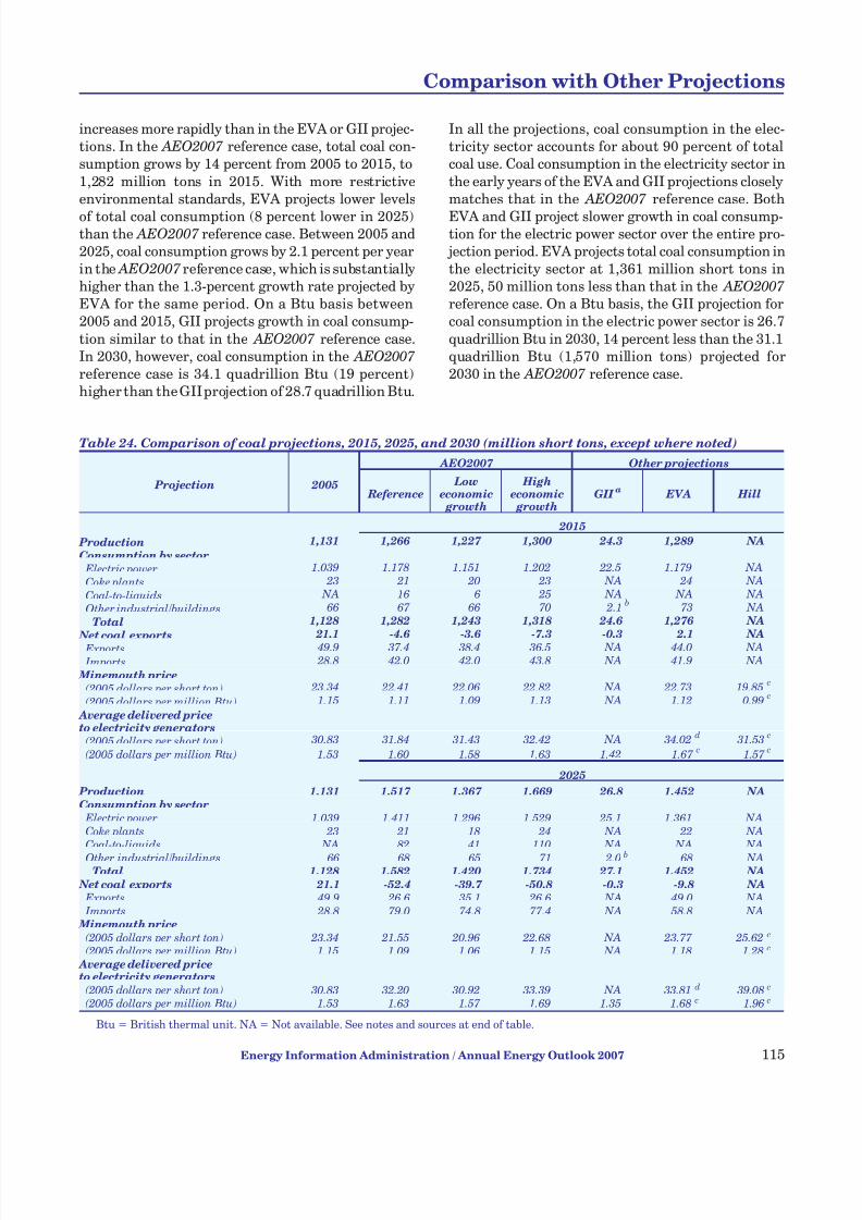
7/28/2019 2007 Annual Energy Outlook
http://slidepdf.com/reader/full/2007-annual-energy-outlook 124/243
increases more rapidly than in the EVA or GII projec-tions. In the AEO2007 reference case, total coal con-sumption grows by 14 percent from 2005 to 2015, to
1,282 million tons in 2015. With more restrictiveenvironmental standards, EVA projects lower levels
of total coal consumption (8 percent lower in 2025)than the AEO2007 reference case. Between 2005 and2025, coal consumption grows by 2.1 percent per yearin the AEO2007 reference case, which is substantiallyhigher than the 1.3-percent growth rate projected byEVA for the same period. On a Btu basis between2005 and 2015, GII projects growth in coal consump-
tion similar to that in the AEO2007 reference case.In 2030, however, coal consumption in the AEO2007
reference case is 34.1 quadrillion Btu (19 percent)higher than the GII projection of 28.7 quadrillion Btu.
In all the projections, coal consumption in the elec-tricity sector accounts for about 90 percent of totalcoal use. Coal consumption in the electricity sector in
the early years of the EVA and GII projections closelymatches that in the AEO2007 reference case. Both
EVA and GII project slower growth in coal consump-tion for the electric power sector over the entire pro-
jection period. EVA projects total coal consumption inthe electricity sector at 1,361 million short tons in2025, 50 million tons less than that in the AEO2007
reference case. On a Btu basis, the GII projection forcoal consumption in the electric power sector is 26.7
quadrillion Btu in 2030, 14 percent less than the 31.1quadrillion Btu (1,570 million tons) projected for2030 in the AEO2007 reference case.
Energy Information Administration / Annual Energy Outlook 2007 115
Comparison with Other Projections
Table 24. Comparison of coal projections, 2015, 2025, and 2030 (million short tons, except where noted)
Projection 2005
AEO2007 Other projections
Reference Low
economic growth
High economic
growthGII a EVA Hill
2015
Production 1,131 1,266 1,227 1,300 24.3 1,289 NA
Consumption by sector Electric power 1,039 1,178 1,151 1,202 22.5 1,179 NA
Coke plants 23 21 20 23 NA 24 NA
Coal-to-liquids NA 16 6 25 NA NA NA
Other industrial/buildings 66 67 66 70 2.1b
73 NA
Total 1,128 1,282 1,243 1,318 24.6 1,276 NA
Net coal exports21.1 -4.6 -3.6 -7.3 -0.3 2.1 NA
Exports 49.9 37.4 38.4 36.5 NA 44.0 NA
Imports 28.8 42.0 42.0 43.8 NA 41.9 NA
Minemouth price(2005 dollars per short ton) 23.34 22.41 22.06 22.82 NA 22.73 19.85
c
(2005 dollars per million Btu) 1.15 1.11 1.09 1.13 NA 1.12 0.99 c
Average delivered priceto electricity generators
(2005 dollars per short ton) 30.83 31.84 31.43 32.42 NA 34.02d
31.53 c
(2005 dollars per million Btu) 1.53 1.60 1.58 1.63 1.42 1.67 c
1.57 c
2025
Production 1,131 1,517 1,367 1,669 26.8 1,452 NAConsumption by sector Electric power 1,039 1,411 1,296 1,529 25.1 1,361 NACoke plants 23 21 18 24 NA 22 NACoal-to-liquids NA 82 41 110 NA NA NA
Other industrial/buildings 66 68 65 71 2.0 b 68 NATotal 1,128 1,582 1,420 1,734 27.1 1,452 NA
Net coal exports 21.1 -52.4 -39.7 -50.8 -0.3 -9.8 NA Exports 49.9 26.6 35.1 26.6 NA 49.0 NA Imports 28.8 79.0 74.8 77.4 NA 58.8 NA
Minemouth price(2005 dollars per short ton) 23.34 21.55 20.96 22.68 NA 23.77 25.62 c
(2005 dollars per million Btu) 1.15 1.09 1.06 1.15 NA 1.18 1.28 c
Average delivered priceto electricity generators
(2005 dollars per short ton) 30.83 32.20 30.92 33.39 NA 33.81 d 39.08 c
(2005 dollars per million Btu) 1.53 1.63 1.57 1.69 1.35 1.68 c 1.96 c
Btu = British thermal unit. NA = Not available. See notes and sources at end of table.
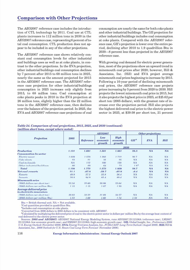
7/28/2019 2007 Annual Energy Outlook
http://slidepdf.com/reader/full/2007-annual-energy-outlook 125/243
The AEO2007 reference case includes the introduc-tion of CTL technology by 2011. Coal use at CTLplants increases to 112 million tons in 2030 in the
AEO2007 reference case, representing 6 percent of to-tal coal consumption. CTL production does not ap-
pear to be included in any of the other projections.
The AEO2007 reference case shows relatively con-stant coal consumption levels for other industrialand buildings uses as well as at coke plants, in con-
trast to the other projections. In the EVA projection,other industrial/buildings coal consumption declinesby 7 percent after 2015 to 68 million tons in 2025,nearly the same as the amount projected for 2015in the AEO2007 reference case. The AEO2007 refer-ence case projection for other industrial/buildingsconsumption in 2025 increases only slightly from
2015, to 68 million tons. Coal consumption atcoke plants peaks in 2010 in the EVA projection at
26 million tons, slightly higher than the 22 milliontons in the AEO2007 reference case, then declinesover the balance of the projection period. In 2025, theEVA and AEO2007 reference case projections of coal
consumption are nearly the same for both coke plantsand other industrial/buildings. The GII projection forother industrial/buildings includes coal consumption
at coke plants. Compared with the AEO2007 refer-ence case, GII’s projection is lower over the entire pe-
riod, declining after 2010 to 1.9 quadrillion Btu in2030—8 percent less than projected in the AEO2007
reference case.
With growing coal demand for electric power genera-
tion, most of the projections show an upward trend inminemouth coal prices after 2020; however, Hill &
Associates, Inc. (Hill) and EVA project averageminemouth coal prices beginning to increase by 2015.Following a 10-year period of declining minemouthcoal prices, the AEO2007 reference case projectsprices increasing by 5 percent from 2020 to 2030. Hill
projects the lowest minemouth coal price in 2015, butit also projects the highest price in 2025, at $25.62 per
short ton (2005 dollars), with the greatest rate of in-crease over the projection period. Hill also projectsthe highest delivered coal price to the electric powersector in 2025, at $39.08 per short ton, 21 percent
116 Energy Information Administration / Annual Energy Outlook 2007
Comparison with Other Projections
Table 24. Comparison of coal projections, 2015, 2025, and 2030 (continued)
(million short tons, except where noted)
Projection 2005
AEO2007 Other projections
Reference Low
economic growth
High economic
growthGII
a EVA Hill
2030
Production 1,131 1,691 1,501 1,861 28.3 NA NAConsumption by sector Electric power 1,039 1,570 1,393 1,712 26.7 NA NACoke plants 23 21 16 25 NA NA NACoal-to-liquids NA 112 100 130 NA NA NAOther industrial/buildings 66 69 64 73 1.9 b NA NA
Total 1,128 1,772 1,573 1,939 28.7 NA NA Net coal exports 21.1 -67.8 -59.7 -62.9 -0.4 NA NA
Exports 49.9 27.2 25.8 26.4 NA NA NA Imports 28.8 94.9 85.4 89.4 NA NA NA
Minemouth price(2005 dollars per short ton) 23.34 22.60 20.99 23.64 NA NA NA(2005 dollars per million Btu) 1.15 1.15 1.07 1.20 NA NA NA
Average delivered priceto electricity generators
(2005 dollars per short ton) 30.83 33.52 31.69 34.57 NA NA NA(2005 dollars per million Btu) 1.53 1.69 1.60 1.74 1.34 NA NA
Btu = British thermal unit. NA = Not available.a Coal quantities provided in quadrillion Btu.bIncludes coal consumption at coke plants.cConverted from 2006 dollars to 2005 dollars to be consistent with AEO2007 .dCalculated by multiplying the delivered price of coal to the electric power sector in dollars per million Btu by the average heat content of
coal delivered to the electric power sector.Sources: 2005 and AEO2007: AEO2007 National Energy Modeling System, runs AEO2007.D112106A (reference case), LM2007.
D112106A (low economic growth case), and HM2007.D112106A (high economic growth case). GII: Global Insight, Inc., Preliminary 2006U.S. Energy Outlook (November 2006). EVA: Energy Ventures Analysis, Inc., FUELCAST: Long-Term Outlook (August 2006). Hill: Hill &
Associates, Inc., 2006 Outlook for U.S. Steam Coal Long-Term Forecast (November 2006).

7/28/2019 2007 Annual Energy Outlook
http://slidepdf.com/reader/full/2007-annual-energy-outlook 126/243
greater than in the AEO2007 reference case. In con-trast to the other projections, GII projects declining delivered coal prices to the electric power sector
through 2030, falling from $1.53 per million Btu(2005 dollars) in 2010 to $1.34 per million Btu in
2030—$0.26 per million Btu (16 percent) less than inthe AEO2007 low economic growth case.
Coal demand is met primarily through domestic pro-duction in all the projections. Both the AEO2007 and
EVA projections show U.S. coal production increasing at an average rate of just over 1 percent per year from2005 to 2015. EVA projects coal production in 2025 at1,452 million short tons, 65 million short tons (4 per-cent) less than in the AEO2007 reference case. The AEO2007 reference case shows the largest increase incoal production over the entire projection period, with
output reaching 1,691 million tons in 2030, nearly 50percent higher than in 2005. The GII projection for
coal production in 2030 is 5.1 quadrillion Btu (15 per-cent) below the AEO2007 reference case projection,
at a level below that in the AEO2007 low economicgrowth case.
U.S. coal exports represent a small percentage of do-mestic coal production in all the projections. EVA pro-
jects the highest level of coal exports, 49 million tonsin 2025, but in contrast with the other projectionsshows exports growing after 2010. Coal exports de-cline to 27 million short tons or less in 2030 in all the
AEO2007 cases. On a Btu basis, coal exports in the
GII projection are lower than those in the AEO2007
reference case in 2030. All the projections expect theUnited States to become a net importer of coal by2020, with the AEO2007 and GII projections antici-pating the transition by 2015. U.S. coal imports reach59 million tons in 2025 in the EVA projection, 20 mil-lion tons less than projected in the AEO2007 refer-
ence case. The AEO2007 reference case projects thehighest level of coal imports, more than tripling over
the projection period to 95 million tons in 2030.
Energy Information Administration / Annual Energy Outlook 2007 117
Comparison with Other Projections
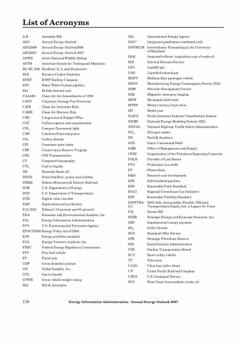
7/28/2019 2007 Annual Energy Outlook
http://slidepdf.com/reader/full/2007-annual-energy-outlook 127/243
A.B. Assembly Bill
AEO Annual Energy Outlook
AEO2006 Annual Energy Outlook2006
AEO2007 Annual Energy Outlook 2007
ANWR Arctic National Wildlife Refuge
ASTM American Society for Testing and Materials
B2, B5, B20 Biodiesel (2, 5, and 20 percent)
BLS Bureau of Labor Statistics
BNSF BNSF Railway Company
BTC Baku-Tbilisi-Ceyhan pipeline
Btu British thermal unit
CAAA90 Clean Air Act Amendments of 1990
CAFE Corporate Average Fuel Economy
CAIR Clean Air Interstate Rule
CAMR Clean Air Mercury Rule
CBO Congressional Budget Office
CCS Carbon capture and sequestration
CFL Compact fluorescent light
CHP Combined heat and power
CO2 Carbon dioxide
CPI Consumer price index
CRP Conservation Reserve Program
CSX CSX Transportation
CT Computed tomography
CTL Coal-to-liquids
DB Deutsche Bank AG
DDGS Dried distillers’ grains and solubles
DM&E Dakota Minnesota & Eastern RailroadDOE U.S. Department of Energy
DOT U.S. Department of Transportation
DVR Digital video recorder
E&P Exploration and production
E10, E85 Ethanol (10 percent and 85 percent)
EEA Economic and Environmental Analysis, Inc.
EIA Energy Information Administration
EPA U.S. Environmental Protection Agency
EPACT2005 Energy Policy Act of 2005
EPS Energy portfolio standard
EVA Energy Ventures Analysis, Inc.
FERC Federal Energy Regulatory Commission
FFV Flex-fuel vehicle
FY Fiscal year
GDP Gross domestic product
GII Global Insights, Inc.
GTL Gas-to-liquids
GVWR Gross vehicle weight rating
Hill Hill & Associates
IEA International Energy Agency
IGCC Integrated gasification combined cycle
INFORUM Interindustry Forecasting at the Universityof Maryland
IRAC Imported refiners’ acquisition cost of crude oil
IRS Internal Revenue Service
LFG Landfill gas
LNG Liquefied natural gas
MDPV Medium-duty passenger vehicle
MECS Manufacturing Energy Consumption Survey (EIA)
MMS Minerals Management Service
MRI Magnetic resonance imaging
MSW Municipal solid waste
MTBE Methyl tertiary butyl ether
MY Model year
NAICS North American Industry Classification System
NEMS National Energy Modeling System (EIA)NHTSA National Highway Traffic Safety Administration
NOx Nitrogen oxides
NS Norfolk Southern
OCS Outer Continental Shelf
OMB Office of Management and Budget
OPEC Organization of the Petroleum Exporting Countries
POLR Provider of Last Resort
PTC Production tax credit
PV Photovoltaic
R&D Research and development
RFG Reformulated gasoline
RFS Renewable Fuels Standard
RGGI Regional Greenhouse Gas Initiative
RPS Renewable Portfolio Standard
SAFETEA- 2005 Safe, Accountable, Flexible, EfficientLU Transportation Equity Act: A Legacy for Users
S.B. Senate Bill
SEER Strategic Energy and Economic Research, Inc.
SEP Supplemental energy payment
SO2 Sulfur dioxide
SOS Standard Offer Service
SPR Strategic Petroleum Reserve
SSA Social Security AdministrationSTB Surface Transportation Board
SUV Sport utility vehicle
TV Television
ULSD Ultra-low-sulfur diesel
UP Union Pacific Railroad Company
USGS U.S. Geological Survey
WTI West Texas Intermediate (crude oil)
118 Energy Information Administration / Annual Energy Outlook 2007
List of Acronyms

7/28/2019 2007 Annual Energy Outlook
http://slidepdf.com/reader/full/2007-annual-energy-outlook 128/243
Text Notes
Overview
Legislation and Regulations
Energy Information Administration / Annual Energy Outlook 2007 119
Notes and Sources
1.For the complete text of the Energy Policy Act of 2005,see web site http://frwebgate.access.gpo.gov/cgi-bin/
getdoc.cgi?dbname=109_cong_public_laws&docid=f:publ058.109.pdf.
2.Full hybrids include an integrated starter-generatorthat allows improved efficiency by shutting the engineoff when the vehicle is idling and an electric motor thatprovides tractive power to the vehicle when it is mov-ing. Mild hybrids include only an integrated starter.
3.Energy Information Administration, Impacts of Modeled Recommendations of the National Commis- sion on Energy Policy, SR/OIAF/2005-02 (Washington,DC, April 2005), web site www.eia.doe.gov/oiaf/ servicerpt/bingaman, and Energy Market Impacts of
Alternative Greenhouse Gas Intensity ReductionGoals, SR/OIAF/2006-01 (Washington, DC, March
2006), web site www.eia.doe.gov/oiaf/service_rpts.htm.
4.E85 is a fuel containing a blend of 70 to 85 percent eth-anol and 30 to 15 percent gasoline by volume.
5.The ethanol tax credit was first established in 1978. Ithas been extended in 1980, 1983,1984, 1990, 1998,and2005.
6.The PTC was subsequently extended in 1999, 2002,2004, and 2005. Some extensions have included signifi-cant modifications, including changes in eligibleresources, changes in the value and duration of the
credit for certain resources, and changes in the treat-ment of the credit with respect to the Alternative Mini-mum Tax.
7.Regional Greenhouse Gas Initiative, “Model Rule & Amended Memorandum of Understanding” (August2006), web site www.rggi.org/modelrule.htm.
8.Regional Greenhouse Gas Initiative, “Memorandum of Understanding” (December 2005), web site www.rggi.org/agreement.htm.
9.For the complete text of the Energy Policy Act of 2005,see web site http://frwebgate.access.gpo.gov/cgi-bin/ getdoc.cgi?dbname=109_cong_public_laws&docid=f:publ058.109.pdf.
10.Energy Information Administration, “EPACT2005
Summary,” Annual Energy Outlook 2006, DOE/EIA-0383(2006) (Washington, DC, February 2006), pp.15-22, web site www.eia.doe.gov/oiaf/archive/aeo06.
11.See, for example, web site http://energy.senate.gov/ public/_files/PostConferenceBillSummary.doc.
12.U.S. Department of Transportation, National High-way Traffic Safety Administration, “Average FuelEconomy Standards for Light Trucks Model Years2008-2011,” 49 CFR Parts 523, 533 and 537 (DocketNo. 2006-24306, RIN 2127-AJ61), web site www.nhtsa.dot.gov/staticfiles/DOT/NHTSA/Rulemaking/ Rules/Associated%20Files/2006FinalRule.pdf.
13.Energy Information Administration, “Proposed Revi-sions to Light Truck Fuel Economy Standards,”
Annual Energy Outlook 2006, DOE/EIA-0383(2006)(Washington, DC, February 2006), pp. 23-24, web sitewww.eia.doe.gov/oiaf/archive/aeo06.
14.U.S. Environmental Protection Agency, “Standards of Performance for Stationary Compression IgnitionInternal Combustion Engines,” 40 CFR Parts 60, 85,89, 94, 1039, 1065, and 1068 (EPA-HQ-OAR-2005-0029, FRL-8190-7, RIN 2060-AM82), web site www.epa.gov/fedrgstr/EPA-AIR/2006/July/Day-11/a5968.htm.
15.See Energy Information Administration, “Clean AirNonroad Diesel Rule,” Annual Energy Outlook 2005 ,DOE/EIA-0383(2005) (Washington, DC, February2005), pp. 14-17, web site www.eia.doe.gov/oiaf/ archive/aeo05.
16.Transition regulations apply to engines constructed orordered after July 11, 2005, and manufactured after
April 1, 2006.17.The regulations specify different time tables and limits
for emergency and fire pump engines.
18.Alpha-Gamma Technologies, Inc., “Population andProjection of Stationary Engines” (Memorandum, June 20, 2005), p. 3, web site www.epa.gov/ttn/atw/ nsps/cinsps/nsps_population_projection4.pdf.
19.Energy Policy Act of 2005, Section 1501. For completetext, see web site http://frwebgate.access.gpo.gov/ cgi-bin/getdoc.cgi?dbname=109_cong_public_laws&docid=f:publ058.109.pdf.
20.Energy Information Administration, “Status andImpact of State MTBE Bans” (March 2003), p. 1, website http://tonto.eia.doe.gov/FTPROOT/service/mtbe.
pdf.21.U.S. Environmental Protection Agency, “State
Actions Banning MTBE” (June 2004), web site www.epa.gov/mtbe/420b04009.pdf.
22.The Federal motor fuels excise tax credit for blending ethanol has been in place since 1978, at 51 cents pergallon. Its expiration date has been extended severaltimes by Congress. Most recently, the American JobsCreation Act of 2004, Section 301, extended the creditthrough 2010.
23.U.S. Department of Energy, Energy Efficiency andRenewable Energy, “Federal Fleet Requirements”(May 2006), web site www1.eere.energy.gov/ vehiclesandfuels/epact/federal.
24.The requirement is actually for 2.7 percent oxygen byweight, which corresponds to 7.7 percent ethanol byvolume. See Minnesota Department of Agriculture,“Economic Impact of the Ethanol Industry in Minne-sota” (May 2003), p. 8, web site www.mda.state.mn.us/ ethanol/economicimpact.pdf.
25.State of Hawaii, “New-Fuel.com—Your Source forInformation About Hawaii’s Transition to Ethanol-Blended Fuel,” web site www.hawaii.gov/dbedt/ert/ new-fuel.
26.National Biodiesel Board, “Minnesota Diesel NowContains Two Percent Biodiesel Statewide” (Press

7/28/2019 2007 Annual Energy Outlook
http://slidepdf.com/reader/full/2007-annual-energy-outlook 129/243
120 Energy Information Administration / Annual Energy Outlook 2007
Notes and Sources
Release, September 29, 2005), web site www.biodiesel.org/resources/pressreleases/gen/20050929_mn_mandate_implemented.pdf.
27.National Biodiesel Board, “Washington State AdoptsBiodiesel Requirement” (Press Release, March30, 2006), web site www.biodiesel.org/resources/ pressreleases/gen/20060330_WA_B2.pdf.
28.Green Car Congress, “Louisiana Legislature Passes2% Renewable Fuels Standard” (June 9, 2006), website www.greencarcongress.com/2006/06/louisiana_legis.html.
29.State of Louisiana, “Governor Blanco Signs HB 685”(Press Release, June 12, 2006), web site www.gov.state.la.us/index.cfm?md=newsroom&tmp=detail&articleID=1945.
30.Testimony of Robert Carroll, Deputy Assistant Secre-tary, Tax Analysis, U.S. Department of the Treasury,before the Subcommittee on Highways, Transit, andPipelines, Committee on Transportation and Infra-
structure, U.S. House of Representatives (April 4,2006).
31.Testimony of Donald Marron, Acting Director, Con-gressional Budget Office, before the Subcommittee onHighways, Transit, and Pipelines, Committee onTransportation and Infrastructure, U.S. House of Rep-resentatives (April 4, 2006).
32.The U.S. Department of Defense maintains a detailedcompilation of Federal, State, and local fuel taxes,inspection fees, and other environmental taxes andfees that apply to the sale of fuel. This compilation,which was last updated in August 2006, can befound at web site www.desc.dla.mil/DCM/Files/Taxcompilation 2006-12.doc.
33.The ethanol tax credit was first established in 1978and has been modifiedor extended in 1980, 1983, 1984,1990, 1998, and 2005.
34.D. Nilles, R. Kotrba, J. Williams, and T. Bryan, “A Boost for Biodiesel,” Biodiesel Magazine (August/Sep-tember 2005), web site www.biodieselmagazine.com/ article.jsp?article_id=376.
35.Eligible wind, poultry litter, geothermal, and certainhydroelectric and biomass facilities can claim the full1.9-cent tax credit. Facilities burning eligible wastestreams, including municipal waste, landfill gases,agricultural and landscaping residues, and forestryand mill wastes receive one-half the value of the creditgiven to other facilities, currently 0.95 cents.
36.Expiration on June 30, 1999, reauthorized on Decem-ber 17, 1999; expiration on December 31, 2001,reauthorized on March 9, 2002; expiration on Decem-ber 31, 2003, reauthorized on October 4, 2004.Reauthorized on August 8, 2005, before scheduledexpiration at the end of 2005. Current expirationscheduled for December 31, 2007.
37.Energy Information Administration, “State Renew-able Energy Requirements and Goals: UpdateThrough 2005,” Annual Energy Outlook 2006, DOE/ EIA-0383(2006) (Washington, DC, February 2006),
pp. 24-27, web site www.eia.doe.gov/oiaf/archive/ aeo06.
38.E-mail communication with Ray Williamson, Arizona Corporation Commission, August 28, 2006.
39.Arizona Corporation Commission, “In the Matter of the Proposed Rulemaking for the Renewable EnergyStandard and Tariff Rules,” Docket No. RE-00000C-05-0030, web site www.cc.state.az.us/utility/electric/ RES-03-14-06.pdf (March 14, 2006).
40.California Public Utilities Commission, “RenewableEnergy,” web site www.cpuc.ca.gov/static/energy/ electric/renewableenergy.
41.California Energy Commission, Renewable Energy Program: Overall Program Guidebook, CEC-300-2006-008-F (Sacramento, CA, April 2006), web sitewww.energy.ca.gov/2006publications/CEC-300-2006-008/CEC-300-2006-008-F.pdf.
42.See web sites www.leginfo.ca.gov/pub/bill/sen/sb_0101-0150/sb_107_bill_20060926_history.html and
www.leginfo.ca.gov/pub/bill/sen/sb_0101-0150/sb_107_bill_20060926_chaptered.pdf.
43.State of Connecticut, “An Act Concerning Biomass,”Substitute Senate Bill No. 212, Public Act No. 06-74,web site www.cga.ct.gov/2006/ACT/PA/2006PA-00074-R00SB-00212-PA.htm.
44.State of Maine, “An Act To Enhance Maine’s EnergyIndependence and Security,” Chapter 677, H.P. 1439 -L.D. 2041, web site www.mainelegislature.org/legis/ bills/chapdocs/PUBLIC677.doc.
45.Commonwealth of Massachusetts, Office of Consumer Affairs and Business Regulation, “Policy Statement onthe RPS Eligibility of Retooled Biomass Plants” (Octo-ber 27, 2005), web site www.mass.gov/doer/rps/rps-
pol-stat-elig-biomass.pdf.46.Commonwealth of Massachusetts, Office of Consumer
Affairs and Business Regulation, “Annual RPS Com-pliance Report for 2004” (January 9, 2006), web sitewww.mass.gov/doer/rps/rps-2004annual-rpt.pdf.
47.Public Utilities Commission of Nevada, “Revised Adopted Regulation of the Public Utilities Commissionof Nevada,” LCB File No. R167-05 ( February 23,2006), web site www.leg.state.nv.us/Register/2005Register/R167-05RA.pdf.
48.New Jersey Board of Public Utilities, New Jersey Administrative Code Title 14, Chapter 8, Subchapter2, “Renewable Portfolio Standards (RPS) Rules Adop-tion” (April 13, 2006), web site www.state.nj.us/
bpu/wwwroot/secretary/RPS_148.2.pdf.49.Wisconsin State Legislature, “Engrossed 2005 Senate
Bill 459” (February 22, 2006), web site www.legis.state.wi.us/2005/data/SB-459eng.pdf.
50.Note that the AEO2007 reference case is based on theCalifornia legislative target (as of September 1, 2006)of 10 percent by 2017. Legislation accelerating thedeadline to 2010 was signed into law too late to beincluded in the AEO2007 projections.
51. Federal Register, Vol. 70, No. 91 (May 12, 2005), 40CFR Parts 51, 72, 73, 74, 77, 78, and 96.

7/28/2019 2007 Annual Energy Outlook
http://slidepdf.com/reader/full/2007-annual-energy-outlook 130/243
Issues in Focus
Energy Information Administration / Annual Energy Outlook 2007 121
Notes and Sources
52. Federal Register, Vol. 70, No. 95 (May 18, 2005), 40CFR Parts 60, 72, and 75.
53.Energy Information Administration, “Federal AirEmissions Regulations,” Annual Energy Outlook
2006, DOE/EIA-0383(2006) (Washington, DC, Febru-ary 2006), pp. 28-29, web site www.eia.doe.gov/oiaf/ archive/aeo06.
54.State and Territorial Air Pollution Program Adminis-trators (STAPPA) and the Association of Local Air Pol-lution Control Officials (ALAPCO), “State MercuryPrograms for Utilities” (August/September 2006), website www.4cleanair.org/StateTable.doc.
55.State of Maine, “States Reach Agreement on ProposedRules for the Nation’s First Cap-and-Trade Programto Address Climate Change” (Press Release, August15, 2006), web site http://mobile.maine.gov/news/ ?sid=22966.
56.M. Finnegan and M. Lifsher, “State’s Greenhouse GasBill Signed,” Los Angeles Times (September 27, 2006).
57.F. Barringer, “Officials Reach California Deal To CutEmissions,” New York Times (August 31, 2006).
58.West Coast Governors’ Global Warming Initiative,web site www.ef.org/westcoastclimate.
59.The AEO2007 near-term world oil prices (for 2006 and2007) are those published in EIA’s September 2006Short-Term Energy Outlook, web site www.eia.doe.gov/pub/forecasting/steo/oldsteos/sep06.pdf.
60.The USGS provides three point estimates for undis-covered and inferred resources: the mean, a 5-percentconfidence interval, and a 95-percent confidence inter-
val, with no price relationship. AEO2007 assumes thatproven reserves are not subject to much uncertainty.
61.Includes crude oil, condensates, natural gas liquids,and refinery gains.
62.M.S. Crandall, Energy, Economics, and Politics in theCaspian Region (Westport, CT: Praeger SecurityInternational, 2006), p. 64.
63.International Energy Agency, Oil Market Report(October 6, 2006), p. 24, web site http://omrpublic.iea.org.
64.BP, Statistical Review of World Energy 2006, web sitewww.bp.com/productlanding.do?categoryId=6842&contentId=7021390 (October 12, 2006).
65.Global Insight, “Brazil Country Brief” (October 18,2006).
66.International Energy Agency, Oil Market Report(October 6, 2006), p. 22, web site http://omrpublic.iea.org.
67.American Petroleum Institute, Joint Association Sur-
vey on Drilling Costs (1996-2004), web site www.api.org/statistics/accessapi/surveys/survey-description.cfm.
68.This well category—that is, a natural gas developmentwell drilled between 7,500 feet and 9,999 feet—waschosen because: (1) about 75 percent of the wells
drilled in the United States are natural gas wells; (2)more than 18 development wells are drilled for everyexploration well; (3) exploration wells can have signifi-cant and unforeseen cost overruns, whereas the drill-ing of development wells is a more routine operation;and (4) the depth category of 7,500 to 9,999 feet
accounts for the greatest number and proportion of natural gas development wells drilled. Consequently,this category is reasonably representative of the oilindustry overall.
69.ODS-Petrodata, Inc., web site https://www.ods-petrodata.com/RigPoint.
70. Oil & Gas Journal, Nelson-Farrar Cost Indices (pub-lished quarterly in January, April, July, and October).
71.Source: Bureau of Labor Statistics, Seasonally Adjusted Producer Price Indices (PPI), Series WPS101. In May 2002, the iron and steel PPI was112.9; by June 2006 it had risen to 194.0(preliminary).
72.Baker-Hughes, Inc., “North American Rotary Rig
Count,” web site www.bhinet.com/investor/rig/rig_na.htm.
73.U.S. Census Bureau, web site www.census.gov/ industry/ma333f05.xls, product code 3331311 forunderground mining machinery.
74.Peabody Energy, Inc., web site www.peabodyenergy.com/pdfs/05_AR_FINANCIALS.pdf.
75.Peabody Energy, Inc., web site www.peabodyenergy.com/pdfs/05_AR_FINANCIALS.pdf.
76.CONSOL Energy, web site http://media.corporate-ir.net/media_files/irol/66/66439/pdfs/AR05.pdf.
77.Massey Energy Company, web site http://library.corporate-ir.net/library/ 10/102/102864/items/195646/ 2005AR.pdf.
78.The subsidiaries of Joy Global manufacture mining machinery that includes continuous miners, longwallshearers, powered roof supports, armored face convey-ors, shuttle cars, flexible conveyor trains, roof bolters,electric mining shovels, rotary blasthole drills, andwalking draglines.
79.R. Barrett, “Mining Boom Brightens Joy GlobalProfits, Developments in China, Milwaukee Journal
Sentinel (February 25, 2005).
80.BNSF Railway, 2005 Annual Report, web site www.bnsf.com/investors/annualreports/2005annrpt.pdf.
81.BNSF Railway, 2005 Annual Report, web site www.bnsf.com/investors/annualreports/2005annrpt.pdf.
82.Toby Kolstad, Rail Theory Forecasts, LLC, personalcommunication, October 22, 2006.
83.“Acquisitions by Railroads and Others,” Progressive
Railroading, Vol. 48, No. 5 (May 2005), p. 49.
84.Imputed from the number and value of backloggedorders reported in Freight Car America’s 2005 AnnualReport, web site www.johnstownamerica.com.
85.Freight Car America, 2005 Annual Report, web sitewww.johnstownamerica.com.
86.P. Foran, “Powergrabs: Traffic Volumes Prompt Rail-roads To Pursue Locomotive Power—and Lots of It,”

7/28/2019 2007 Annual Energy Outlook
http://slidepdf.com/reader/full/2007-annual-energy-outlook 131/243
122 Energy Information Administration / Annual Energy Outlook 2007
Notes and Sources
Progressive Railroading, Vol.48, No. 5 (May2005), pp.50-51.
87.BNSF Railway, 2005 Annual Report, web site www.bnsf.com/investors/annualreports/2005annrpt.pdf.
88.Surface Transportation Board, U.S. Department of Transportation, “Statistics of Class I Freight Rail-roads in the United States,” web site www.stb.dot.gov/ econdata.nsf.
89.BNSF Railway, 2005 Annual Report, web site www.bnsf.com/investors/annualreports/2005annrpt.pdf.
90.Reviews of energy demand elasticities include C. Dahl, A Survey of Energy Demand Elasticities in Support of
the Development of the NEMS, Contract NumberDE-AP01-93EI23499 (Washington, DC, October1993).
91.Federal Energy Regulatory Commission, Assessment
of Demand Response and Advanced Metering, Staff Report, Docket AD-06-2-000 (Washington, DC, August2006), web site www.ferc.gov/legal/staff-reports/
demand-response.pdf.92.Energy Information Administration, Commercial
Buildings Energy Consumption Survey (2003 data),web site www.eia.doe.gov/emeu/cbecs.
93.L.J. Sandahl, T.L. Gilbride, M.R. Ledbetter, H.E.Steward, and C. Calwell, Compact Fluorescent
Lighting in America: Lessons Learned on the Way to Market, PNNL-15730 (Richland, WA: Pacific North-west National Laboratory, June 2006), web sitewww.eere.energy.gov/buildings/info/documents/pdfs/ cfl_lessons_learned_web.pdf.
94.Web sites www.energystar.gov and www.eere.energy.gov/buildings/building_america.
95.K.A. Hanson, “Seasonality of Moves and Duration of
Residence,” U.S. Census Bureau, Current PopulationReports, Household Economic Studies (October 1998),web site www.census.gov/prod/3/98pubs/p70-66.pdf.
96.R. Nevin and G. Watson, “Evidence of Rational Market Valuations for Home Energy Efficiency,” Appraisal
Journal (October 1998).
97.Apparently, some very low-cost projects are neverundertaken. See S.T. Anderson and R.G. Newell,“Information Programs for Technology Adoption: TheCase of Energy-Efficiency Audits,” Resource and
Energy Economics, Vol. 26, No. 1 (March 2004),pp. 27-50. See web site www.rff.org/~newell/ ResEnergyEcon.pdf.
98.R.B. Lung, A. McKane, and M. Olszewski, “Industrial
Motor System Optimization Projects in the US: AnImpact Study,” TAPPI, web site www.tappi.org/ s_tappi/sec_publications.asp?CID=4583&DID=510344; and U.S. Department of Energy, Office of Industrial Technologies, “Georgia Pacific’s InsulationUpgrade Leads to Reduced Fuel Costs and IncreasedProcess Efficiency,” web site www1.eere.energy.gov/ industry/bestpractices/pdfs/insulation.pdf.
99.Based on data from the U.S. Census Bureau’s 2004 Annual Survey of Manufactures, published in Statis-
tics for Industry Groups and Industries: 2004,
M04(AS)-1 (Washington, DC, December 2005), website www.census.gov/mcd/asm-as1.html.
100.Based on data from EIA’s 2002 Manufacturing EnergyConsumption Survey (MECS), Tables 10.2 to 10.13,web site www.eia.doe.gov/emeu/mecs/mecs2002/ data02/shelltables.html. Petrochemical feedstocks arenot reported separately in MECS but are included inthis calculation.
101.See W.A. Pizer, W. Harrington, R.J. Kopp, R.D.Morgenstern, and J-S Shih, “Technology Adoption and Aggregate Energy Efficiency,” Discussion Paper 02-52(Washington, DC: Resources for the Future, December2002), web site www.rff.org/Documents/RFF-DP-02-52.pdf.
102.Electricity demand for commercial office equipment isan end-use category separate from miscellaneous con-sumption.
103.TIAX LLC, Commercial and Residential Sector Miscel-laneous Electricity Consumption: Y2005 and Projec-
tions to 2030 , EIA contract report (September 2006).104.The decline in electricity use per unit is driven by thenew California standard that requires less electricityuse while in standby mode, which accounts for morethan 99 percent of hours of use over the course of a year. See California Energy Commission, 2006 Appli-ance Efficiency Regulations, CEC-400-2006-002 (Sac-ramento, CA, January 2006).
105.Alaska’s former governor, Frank Murkowski, sup-ported 20-percent equity ownership for the State,which would also bear 20 percent of the constructioncosts.
106.The Northern Pipeline Act awarded Foothills PipeLines Ltd. the certificate for construction of the Cana-
dian portion of the Alaska Natural Gas TransportationSystem along the Alaska Highway. After the passage of the Northern Pipeline Act, TransCanada purchasedFoothills Pipe Line.
107.BP, ExxonMobil, and ConocoPhillips, “Alaska Pro-ducer Pipeline Update” (May 2002), Slide 15, web sitewww.arcticgaspipeline.com/Reference/Documents&Presentations/ProducerInformation/5-02Alaska ProducerUpdate.ppt.
108.U.S. Department of Labor, Bureau of Labor Statistics,Seasonally Adjusted Producer Price Indices (PPI),Series WPS101. In May 2002 the PPI for iron and steelwas 112.9; in June 2006 it was 194.0.
109.Energy Information Administration, “Coal Distribu-
tion Back Issues,” web site www.eia.doe.gov/cneaf/ coal/page/coaldistrib/coal_distributions.html.
110.EIA’s coal distribution data for 2004 indicate that themode of transportation for 28 million tons (3 percent)of domestic coal shipments was “unknown.”
111.Energy Information Administration, “Coal Transpor-tation: Rates and Trends in the United States,1979-2001 (with Supplementary Data to 2002),”Table 2.06, web site www.eia.doe.gov/cneaf/coal/page/ trans/ratesntrends.html.

7/28/2019 2007 Annual Energy Outlook
http://slidepdf.com/reader/full/2007-annual-energy-outlook 132/243
Energy Information Administration / Annual Energy Outlook 2007 123
Notes and Sources
112.U.S. Senate, Committee on Energy and NaturalResources, “Coal-Based Generation Reliability,”Statement of David Wilks, President of Energy Sup-ply, Xcel Energy, on behalf of the Edison Electric Insti-tute and Consumers United for Rail Equity (May 25,2006).
113.Average transportation rates are imputed from the dif -ference between average delivered prices, excluding imports, and average minemouth prices.
114.BNSF Railway Company, Quarterly Report (June 30,2006) web site www.bnsf.com/investors/secfilings/ 10Q_Railway_2Q_2006.pdf.
115.U.S. Government Accountability Office, Freight Rail-roads: Industry Health Has Improved, But Concerns
about Competition and Capacity Should Be Addressed,GAO-07-94 (Washington, DC, October 2006), web sitewww.gao.gov/new.items/d0794.pdf.
116.U.S. Senate, Subcommittee on Surface Transportationand Merchant Marine, “Economics, Service and
Capacity in the Freight Railroad Industry,” Statementof W. Douglas Buttrey, Chairman, Surface Transpor-tation Board (June 21, 2006).
117.Surface Transportation Board, web site www.stb.dot.gov.
118.N. Carey, “Margins, Fuel Charges Boost Union Pacific4th Qtr,” Reuters.com (January 2006).
119.Norfolk Southern, web site www.nscorp.com/ nscorphtml/marketing/pricing/NS8003_terms.html.
120.CSX, web site http://shipcsx.com/public/ec.shipcsxpublic/Main?module_url=/ec.pricingpublic/About.
121.Surface Transportation Board Decision, Rail Fuel
Surcharges, Ex Parte No. 661 (August 3, 2006), website www.stb.dot.gov.
122.Surface Transportation Board , Rail Fuel Surcharge,Comments of BNSF Railway (October 2, 2006).
123.“CSX STB Fuel Surcharge Filing” (October 3, 2006)web site www.csx.com.
124.U.S. Senate, Committee on Energy and NaturalResources, “Coal-Based Generation Reliability,”Statement of Howard Gruenspecht, Deputy Adminis-trator, Energy Information Administration (May 25,2006).
125.R. Smith and D. Machalaba, “As Utilities Seek MoreCoal, Railroads Struggle To Deliver,“ Wall Street Jour-
nal (March 15, 2006), p. A1; and “Coal Stocks Outper-form S&P, Metals Securities,” Platts Coal Trader(November 15, 2005), pp. 2-3.
126.S. Bobb, Group Vice President of Coal Marketing,BNSF Railway, “June 2006 Coal Update,” paper pre-sented to staff at the Energy Information Administra-tion (Washington, DC, June 27, 2006).
127.U.S. Senate, Committee on Energy and NaturalResources, “Coal-Based Generation Reliability,”Statement of Edward Hamberger, President and Chief Executive Officer, Association of American Railroads(May 15, 2006); and S. Bobb, Group Vice President of Coal Marketing, BNSF Railway, “June 2006 CoalUpdate,” paper presented to staff at the Energy Infor-
mation Administration (Washington, DC, June 27,2006).
128.A.J. Cebula, Vice President of Planning & Engi-neering, CANAC Inc., “Southern Powder River Basin,BNSF/UP Joint Line, Towards Sustainable Opera-tions of 500 mmT,” paper presented at the NationalCoal Transportation Association Annual Fall Meeting & Conference (Denver, CO, September 13, 2006).
129.“CANAC Sees 50 Percent Jump in SPRB Output by2012,” Argus Coal Transportation, Vol. 25, No. 17(September 14, 2006), p. 1.
130.Personal communication to EIA from Doug Conway,General Manager–Coal, DM&E and IC&E Railroads(November 16, 2006).
131.O. Port, “Not Your Father’s Ethanol,” Business Week(February 21, 2005), web site www.businessweek.com/ magazine/content/05_08/b3921117.htm.
132.National Renewable Energy Laboratory, Ligno-
cellulosic Biomass to Ethanol Process Design and Eco-
nomics Utilizing Co-Current Dilute Acid Prehydrolysisand Enzymatic Hydrolysis for Corn Stover, NREL/ TP-510-32438 (Golden, CO, June 2002), web site www.nrel.gov/docs/fy02osti/32438.pdf.
133.National Biodiesel Board, “Biodiesel—Commonly Asked Questions,” web site www.nbb.org/pdf_files/ fuelfactsheets/CommonlyAsked.PDF.
134.U.S. Department of Energy, Energy Efficiency andRenewable Energy, Alternative Fuels Data Center,“State and Federal Incentives and Laws,” web sitewww.eere.energy.gov/afdc/progs/view_ind_mtx.cgi?in/ TAX/US/0.
135.U.S. Department of Agriculture, The Economic Feasi-
bility of Ethanol Production from Sugar in the United
States (Washington, DC, July 2006), Table 19, web sitewww.usda.gov/oce/EthanolSugarFeasibilityReport3.pdf.
136.U.S. Department of Agriculture, USDA’s 2002 Etha-
nol Cost-of-Production Survey (Washington, DC, July2005), Table 3, web site www.usda.gov/oce/reports/ energy/USDA_2002_ETHANOL.pdf.
137.Promar International, Evaluation and Analysis of
Vegetable Oil Market: The Implication of Increased Demand for Industrial Uses on Markets & USB Strat-
egy (November 2005), pp. 37-41, web site www.nbb.org/resources/reportsdatabase/reports/gen/20051101_gen-368.pdf.
138.National Renewable Energy Laboratory, Biomass Oil
Analysis: Research Needs and Recommendations,NREL/TP-510-34796 (June 2004), Table 23, web sitewww.nrel.gov/docs/fy04osti/34796.pdf.
139.In 2005, the wholesale price of gasoline was imputed tobe $1.74 per gallon and the wholesale price of diesel$1.78 per gallon. In 2012, the average U.S. wholesaleprices are projected to be $1.52 and $ 1.48 per gallon,respectively, as some of the unusual margins of therefinery market are projected to return to the histori-cal pattern.
140.U.S. Department of Agriculture, USDA’s 2002 Etha-nol Cost-of-Production Survey (Washington, DC, July

7/28/2019 2007 Annual Energy Outlook
http://slidepdf.com/reader/full/2007-annual-energy-outlook 133/243
Market Trends
124 Energy Information Administration / Annual Energy Outlook 2007
Notes and Sources
2005), Table 3, web site www.usda.gov/oce/reports/ energy/USDA_2002_ETHANOL.pdf.
141.S. Howell, “Time To Take the Biodiesel Plunge?” Ren-
der Magazine (February 2005), pp. 10-14.
142.R. Pruszko, “Rendered Fats and Oils as a Biodiesel
Feedstock: The Opportunities and Challenges,” Ren-der Magazine (February 2006), pp. 10-12.
143.K. Collins, Chief Economist, U.S. Department of Agri-culture, “Statement Before the U.S. Senate Commit-tee on Agriculture, Nutrition, and Forestry” (January10, 2007), p. 2, web site www.usda.gov/oce/newsroom/ congressional_testimony/Collins_011007.pdf.
144.A. Baker and S. Zahniser, “Ethanol Reshapes the CornMarket,” Amber Waves Magazine, Vol. 4, No. 2 (2006),pp. 30-35, web site www.ers.usda.gov/AmberWaves/ April06/Features/Ethanol.htm.
145.Promar International, Evaluation and Analysis of Vegetable Oil Market: The Implication of Increased
Demand for Industrial Uses on Markets & USB Strat-
egy (November 2005), pp. 25-35, web site www.nbb.org/resources/reportsdatabase/reports/gen/20051101_gen-368.pdf.
146.U.S. Department of Agriculture, 2002 Census of Agri-
culture (Washington, DC, June 2004), Vol. 1, Chapter1, “U.S. National Level Data,” Table 8, “Land: 2002and 1997,” web site www.nass.usda.gov/census/ census02/volume1/us/st99_1_008_008.pdf.
147.U.S. Department of Agriculture, Summary Report:1997 National Resources Inventory (Washington, DC,December 2000), Figure 1, “How Our Land Is Used,1997,” web site www.nrcs.usda.gov/Technical/NRI/ 1997/summary_report/figures.html#figure1.
148.For a description of the Conservation Reserve Pro-
gram, see web site www.nrcs.usda.gov/programs/crp.149.U.S. Department of Agriculture, Baseline Projection
(Washington, DC, February 2006), Tables 8 and 13,“Planted Acres, 2005/06 Marketing Year.”
150.Historic crop yields tabulated by U.S. Department of Agriculture, National Agriculture Statistics Service,web site www.nass.usda.gov/Data_and_Statistics/ Quick_Stats/index.asp.
151.Average yield increase calculated from 30-year historicdata supplied by U.S. Department of Agriculture,National Agriculture Statistics Service.
152.U.S. Department of Agriculture and U.S. Departmentof Energy, Biomass as a Feedstock for a Bioenergy and
Bioproducts Industry: The Technical Feasibility of a
Billion-Ton Annual Supply, DOE/GO-102995-2135(Washington, DC, April 2005), web site http:// feedstockreview.ornl.gov/pdf/billion_ton_vision.pdf.
153.Renewable Fuels Association, From Niche to Nation:
Ethanol Industry Outlook 2006 (Washington, DC, Feb-ruary 2006), pp. 14-15, web site www.ethanolrfa.org/ objects/pdf/outlook/outlook_2006.pdf.
154.Promar International, Evaluation and Analysis of Vegetable Oil Market: The Implication of Increased
Demand for Industrial Uses on Markets & USB Strat- egy (November 2005), pp. 25-35, web site www.nbb.
org/resources/reportsdatabase/reports/gen/20051101_gen-368.pdf.
155.National Biodiesel Board, “Biodiesel Production,” website www.nbb.org/pdf_files/fuelfactsheets/Production.pdf.
156.F. Luxem, “Glycerin as a C-3 Raw Material,” pre-sented at the 2006 National Biodiesel Conference.
157.National Corn Grower’s Association, “How Much Eth-anol Can Come From Corn?” (May 2006), web sitewww.ncga.com/ethanol/pdfs/2006/HowMuchEthanolCan ComeFromCorn.v.2.pdf.
158.U.S. Department of Agriculture, “Agricultural Base-line Projections 2006-2015,” web site www.ers.usda.gov/Briefing/Baseline/crops.htm.
159.National Corn Growers Association, “U.S. Corn Usageby Segment, 2005” (pie chart), web site www.ncga.com/WorldOfCorn/main/consumption1.asp.
160.U.S. Department of Energy, Energy Efficiency andRenewable Energy, Alternative Fuels Data Center,
web site www.eere.energy.gov/afdc/progs/reg_matrx.cgi.
161.K. Collins, Chief Economist, U.S. Department of Agri-culture, “Statement before the U.S. Senate Committeeon Environment and Public Works” (September 6,2006), p. 8, web site www.usda.gov/oce/newsroom/ congressional_testimony/Biofuels Testimony 9-6-2006.doc.
162.The year 2004 was used as the end point (as opposed to2005, which is the base year of the AEO2007 projec-tions) because of the precipitous drop in industrialenergy consumption between 2004 and 2005 caused by
the impact of hurricanes Katrina and Rita.
163.When the reference case industrial energy intensityprojections are decomposed using the Divisia index,structural change accounts for 61 percent of the pro- jected change in energy intensity. A discussion of theindex can be found in Boyd et al., “Separating theChanging Effects of U.S. Manufacturing Productionfrom Energy Efficiency Improvements,” Energy Jour-nal, Vol. 8, No. 2 (1987).
164.The refining portion of the industrial sector is pro- jected to become more energy-intensive over time. Itsenergy intensity is projected to increase as a result of declining crude oil quality, higher quality products,and the use of alternative inputs and technologies toproduce liquid fuels. Coal-to-liquids and biofuel tech-niques are more energy-intensive than standard refin-ing processes.
165.The alternative technology cases change technologycharacterizations only for sectors represented in theNEMS industrial model. Consequently, in the technol-ogy cases portrayed in Figure 48, refining values areunchanged from those in the reference case projec-tions. The petroleum refining industry displays a range of intensity changes in other alternative AEO-
2007 cases but responds differently from the other

7/28/2019 2007 Annual Energy Outlook
http://slidepdf.com/reader/full/2007-annual-energy-outlook 134/243
Comparison with Other Projections
Table Notes and Sources
Note: Tables indicated as sources in these notes referto the tables in Appendixes A, B, C, and D of this
report.
Table 1. Total energy supply and disposition in the AEO2007 and AEO2006 reference cases, 2005-2030: AEO2006: AEO2006 National Energy Modeling System ,run AEO2006.D111905A. AEO2007 : AEO2007 NationalEnergy Modeling System, run AEO2007.D112106A. Notes:Quantities are derived from historical volumes and as-sumed thermal conversion factors. Other production in-cludes liquid hydrogen, methanol, and some inputs to refin-eries. Net imports of petroleum include crude oil, petroleumproducts, unfinished oils, alcohols, ethers, and blending
components. Other net imports include coal coke and elec-tricity.
Table 2. Changes in Standard Offer Supply price de-terminations by supply region and State: Brubakerand Associates, Inc., “Customer Choice Update: State byState Summary of Restructuring Activities Around the Na-tion,” in Retail Competition Struggles As Fuel Costs Rise
And Rate Caps Expire (Spring 2006), web site www.consultbai.com/publications/newsletter/spring06_newslet-ter.pdf. Energy Information Administration Survey Data:2005 preliminary f-861 database for the Arizona, Connecti-cut, Delaware, District of Columbia, Illinois, Montana, Ne-vada, New Hampshire, New York, Ohio, Oregon, Pennsyl-vania, Rhode Island, and Virginia percent of competitiveload. Energy Information Administration, “Status of State
Electric Industry Restructuring Activity—as of February2003,” web site www.eia.doe.gov/cneaf/electricity/chg_str/ restructure.pdf. Connecticut Department of Public UtilityControl, “Decision: Docket No. 06-01-08PH01, DPUC De-velopment and Review of Standard Service and Supplier of Last Report Service—Phase I” (June 21, 2006). District of Columbia Public Service Commission, “Questions And An-swers Regarding Pepco’s 2004 Request for Proposals forStandard Offer Service, web site www.dcpsc.org/pdf_files/ hottopics/RisingElectricityPrices_FAQ.pdf. Illinois Com-merce Commission, “Electric Switching Statistics” (April
Energy Information Administration / Annual Energy Outlook 2007 125
Notes and Sources
174.Because EVA reports a 2005 price of $8.84 (2005 dol-lars per thousand cubic feet), its projection actuallyshows a greater decline relative to the reported 2005price than does the AEO2007 reference case.
175.A delivered natural gas price margin equals theend-use sector natural gas price minus the wellheadnatural gas price.
176.It should be noted that the 2005 industrial pricereported by the other organizations is about a dollarhigher than that reported in AEO2007 .
industrial subsectors. For example, because of in-creased CTL production in the high price case, energyintensity in the petroleum refining industry is higherthan in the reference case. In all the other industrialsubsectors, energy intensity is lower in the high pricecase.
166.S.C. Davis and S.W. Diegel, Transportation Energy Data Book: Edition 25 , ORNL-6974 (Oak Ridge, TN,May 2006), Chapter 3, “All Highway Vehicles andCharacteristics,” web site http://cta.ornl.gov/data/ chapter3.shtml.
167.Unless otherwise noted, the term “capacity” in the dis-cussion of electricity generation indicates utility,nonutility, and combined heat and power capacity.Costs reflect the weighted average of regional costs.
168.Does not include off-grid photovoltaics (PV). Based onannual PV shipments from 1989 through 2004, EIA estimates that as much as 167 megawatts of remote PV applications for electricity generation (off-grid powersystems) was in service in 2004, plus an additional 447megawatts in communications, transportation, andassorted other non-grid-connected, specialized appli-cations. See Energy Information Administration,
Annual Energy Review 2005 , DOE/EIA-0384(2005)(Washington, DC, July 2006), Table 10.6 (annual PV shipments, 1989-2004). The approach used to developthe estimate, based on shipment data, provides anupper estimate of the size of the PV stock, including both grid-based and off-grid PV. It overestimates thesize of the stock, because shipments include a substan-tial number of units that are exported, and each yearsome of the PV units installed earlier are retired fromservice or abandoned.
169.Avoided cost estimates the incremental cost of fuel andcapacity displaced by a unit of the specified resourceand more accurately reflects its as-dispatched energyvalue than comparison to the levelized cost of otherindividual technologies. It does not reflect system reli-ability cost, nor does it necessarily indicate the lowestcost alternative for meeting system energy and capac-ity needs.
170.Although cellulosic ethanol technology currently is nota commercially proven process, researchers and devel-opers are vigorously pursuing cost reduction goals inthe technology and production processes that wouldsubstantially exceed those considered in the AEO2007 “lower cost” cases. These even lower production costgoals may be possible, but it is uncertain at presentwhether, and when, the technology advances neces-sary to achieve the lowest of the production cost goalswill occur. Nevertheless, even the relatively modestreductions in production costs assumed in the AEO-
2007 “lower cost” cases can be seen to result in a sig-nificant increase in cellulosic ethanol production.
171.CAIR mandates SO2 emissions caps in 28 eastern andmidwestern States and the District of Columbia. Thefirst compliance period begins in 2010, and a second,more stringent cap takes effect in 2015.
172.The first milestone for reducing NOx emissions fromelectric power generation becomes effective in 2009. A lower limit is mandated for 2015.
173.The Phase I mercury cap is 38 short tons, beginning in2010. The Phase II cap is 15 short tons, beginning in2018.

7/28/2019 2007 Annual Energy Outlook
http://slidepdf.com/reader/full/2007-annual-energy-outlook 135/243
2006), web site www.icc.illinois.gov/en/switchstats.aspx.Maine State Legislature, Office of the Revisor of Statutes,“Maine Public Utilities/Standard Offer Law, Title 35-A,Public Utilities, Part 3, Electric Power, Chapter 32, ElectricIndustry Restructuring, §3212,” web site http://janus.state.me.us/legis/statutes/35-A/title35-Asec3212.html.
Maine Public Utility Commission, Standard Offer ServiceRule, Chapter 301, web site http://Mainegov-Images.Informe.Org/Mpuc/Doing_Business/Rules/Part_3/Ch-301.pdf. Maine Public Utilities Commission, “Maine’s LoadServed by Competitive Providers as of June 1, 2006,” website http://mainegov-images.informe.org/mpuc/industries/ electricity/electric%20restructuring/Migration_Rates_Monthly-June06.pdf. Maryland Public Service Commis-sion, Case No. 8908, “In the Matter of the Commission’s In-quiry into the Competitive Selection of Electricity Sup-plier/Standard Offer Service, The Commission Staff’s Re-port/Observations on the Standard Offer Service Bidding Process and Results” (March 7, 2006). Maryland Public Ser-vice Commission, “Electric Choice Enrollment Monthly Re-port” (July 19, 2006), web site www.psc.state.md.us/psc/ electric/enrollmentrpt.htm. Massachusetts Department of Technology and Energy, Electric Restructuring in Massa-chusetts, “Default Service” (2006), web site www.mass.gov/dte/restruct/competition/defaultservice.htm. Massa-chusetts Division of Energy Resources, “2006 ElectricPower Customer Migration Data” (May 2006), web sitewww.mass.gov/Eoca/docs/doer/2006migrate.pdf. MichiganPublic Service Commission, “Electric Customer Choice,Program Status: MPSC Reports on the Status of ElectricCompetition in Michigan, as of July 31, 2006,” web sitewww.dleg.state.mi.us/mpsc/electric/restruct/status.htm.Public Utilities Company of Ohio, “Electric Rate Stabiliza-tion Plans: Ensuring Rate Certainty in Ohio,” web sitewww.puco.ohio.gov/PUCO/Consumer/information.cfm?doc_id=1449. New Hampshire Public Utilities Commis-sion, Electric Division, web site www.puc.state.nh.us/Elec-
tric/electric.htm. New York Public Service Commission,“Mandatory Hourly Pricing,” web site www.dps.state.ny.us/Mandatory_Hourly_Pricing.html. New York PublicService Commission, “Retail Access Plans,” web sitewww.dps.state.ny.us/Retail_Access_Plans.html. New YorkPublic Service Commission, “Staff Report on the State of Competitive Energy Markets: Progress to Date and FutureOpportunities” (March 2, 2006), web site www.dps.state.ny.us/StaffReportCompetition.pdf. New York PublicService Commission, Case 00-M-0504, “Proceeding on Mo-tion of the Commission Regarding Provider of Last ResortResponsibilities: The Role of Utilities in Competitive En-ergy Markets and Fostering Development of Retail Compet-itive Opportunities. Statement of Policy on Further StepsToward Competition in Retail Energy Markets” (August
25, 2004) web site http://www3.dps.state.ny.us/pscweb/ WebFileRoom.nsf/ArticlesByCategory/F4746B665D1C642685256EFB00622E91/$File/201a.00m0504.pdf?OpenElement. Ohio Public Utilities Commission, “The End of theMarket Development Period for Retail Electric Choice,”web site www.puco.ohio.gov/puco/mediaroom/annualpublications.cfm?doc_id=1679#Electric. Oregon PublicUtility Commission, “Competitive Power Market for Ore-gon Business Customers,” web site www.puc.state.or.us/ PUC/electric_restruc/ORDA03-05.pdf. Oregon Public Util-ity Commission, “Restructuring for Residential Con-sumers,” web site www.oregon.gov/PUC/electric_restruc/ consumer/resident.shtml. Oregon Public Utility Commis-
sion, “Status Report: Oregon Electric Industry Restruc-turing,” (September, 2006), web site www.puc.state.or.us/ PUC/electric_restruc/statrpt/2006/092006_status_report.pdf. Pennsylvania Public Utility Commission, “Metropoli-tan Edison Company & Pennsylvania Electric CompanyRate Filing,” “Duquesne Light Company Rate Filing,” and
“Penn Power’s POLR Filing,” web site www.puc.state.pa.us/electric/electric_index.aspx. Pennsylvania Public UtilityCommission, “Provider of Last Resort,” web site www.puc.state.pa.us/electric/electric_last_resort.aspx. Pennsylvania Public Utility Commission, “Rulemaking Re Electric Distri-bution Companies,” Docket No. L-00040169, and “Obliga-tion to Serve Retail Customers at the Conclusion of theTransition Period Pursuant to 66 Pa. C.S. §2807(e)(2), Pro-vider of Last Resort Roundtable, Docket No. M-00041792,Proposed Rulemaking Order” (December 14, 2004), website www.puc.state.pa.us/PcDocs/514337.doc. Texas PublicUtility Commission, “Report to the 79th Texas Legislature:Scope of Competition in Electric Markets in Texas” (Janu-ary 2005), web site www.puc.state.tx.us/electric/reports/ scope/2005/2005scope_elec.pdf.
Table 3. OPEC and non-OPEC oil production inthree AEO2007 world oil price cases, 2005-2030: AEO2007 National Energy Modeling System, runs AEO2007.D112106A, HP2007.D112106A, and LP2007.D112106A; and Energy Information Administration,Short-Term Energy Outlook (September 2006), web sitewww.eia.doe.gov/pub/forecasting/steo/oldsteos/sep06.pdf.
Table 4. Changes in surface coal mining equipmentcosts, 2002-2005: 2002 and 2003: Previous editions, website www.census.gov/cir/www. 2004 and 2005: U.S. De-partment of Commerce, Economics and Statistics Adminis-tration, U.S. Census Bureau, Current Industrial Reports,Construction Machinery: 2005 , MA333D(05)-1 (Washing-ton, DC, July 2006).
Table 5. Miscellaneous electricity uses in the resi-dential sector, 2005, 2015, and 2030: TIAX LLC, “Com-mercial and Residential Sector Miscellaneous ElectricityConsumption: Y2005 and Projections to 2030” (September2006); and AEO2007 National Energy Modeling System,run AEO2007.D112106A.
Table 6. Electricity use and market share for televi-sions by type, 2005 and 2015: TIAX LLC, “Commercialand Residential Sector Miscellaneous Electricity Consump-tion: Y2005 and Projections to 2030” (September 2006).
Table 7. Miscellaneous electricity uses in the com-mercial sector, 2005, 2015, and 2030: TIAX LLC, “Com-mercial and Residential Sector Miscellaneous ElectricityConsumption: Y2005 and Projections to 2030” (September2006); and AEO2007 National Energy Modeling System,
run AEO2007.D112106A.Table 8. Revised subgroups for the non-energy-intensive manufacturing industries in AEO2007 : en-ergy demand and value of shipments, 2002: Office of Management and Budget, North American Industry Classi-
fication System—United States (Springfield, VA, 2002). En-ergy: Energy Information Administration, Manufacturing Energy Consumption Survey 2002. Value of Shipments:Global Insight, Inc., 2006 U.S. Energy Outlook (November2006).
Table 9. Effects of DOE’s loan guarantee program onthe economics of electric power plant generating
126 Energy Information Administration / Annual Energy Outlook 2007
Notes and Sources

7/28/2019 2007 Annual Energy Outlook
http://slidepdf.com/reader/full/2007-annual-energy-outlook 136/243
technologies, 2015: AEO2007 National Energy Modeling System, runs AEO2007.D112106A and NUCLOAN.D020207A.
Table 10. Technically recoverable undiscovered oiland natural gas resources in the lower 48 Outer Con-tinental Shelf as of January 1, 2003: U.S. Department
of the Interior, Minerals Management Service, Report toCongress: Comprehensive Inventory of U.S. OCS Oil and
Natural Gas Resources (February 2006), web site www.mms.gov/revaldiv/PDFs/FinalInvRptToCongress050106.pdf.
Table 11. U.S. motor fuels consumption, 2000-2005:Energy Information Administration, Annual Energy Re-view 2005 , DOE/EIA-0384(2005) (Washington, DC, July2006), Table 5.13c, web site www.eia.doe.gov/emeu/aer; Re-newable Fuels Association, “Industry Statistics 2006,” website www.ethanolrfa.org/industry/statistics; National Bio-diesel Board, “Estimated U.S. Biodiesel Production,” website www.biodiesel.org/pdf_files/fuelfactsheets/Production_Graph_Slide.pdf.
Table 12. Energy content of biofuels: Energy Informa-
tion Administration, Annual Energy Review 2005 , DOE/ EIA-0384(2005) (Washington, DC, July 2006), Table A.1,web site www.eia.doe.gov/emeu/aer; U.S. EnvironmentalProtection Agency, A Comprehensive Analysis of Biodiesel
Impacts on Exhaust Emissions, EPA420-P-02-001 (Wash-ington, DC, October 2002), web site http://65.166.250.34/ resources/reportsdatabase/reports/gen/20021001_gen-323.pdf; Argonne National Laboratory, Center for Transporta-tion Research, GREET 1.5 Transportation Fuel Cycle
Model: Volume 1, Methodology, Development Use and Re- sults,” ANL/ESD-39 (Argonne, IL, August 1999), Table 3.3,web site www.transportation.anl.gov/software/GREET/ pdfs/esd_39v1.pdf. Note: E85 is rarely blended as 85 per-cent ethanol and 15 percent gasoline. The more typicalblend is 77 percent ethanol and 23 percent gasoline, but the
term E85 is still used.Table 13. U.S. production and values of biofuel co-products: U.S. Department of Agriculture, “USDA’s 2002Ethanol Cost-of-Production Survey” (Washington, DC, July 2005), web site www.usda.gov/oce/reports/energy/ USDA_2002_ETHANOL.pdf; USDA NASS Statistical Da-tabase, web site www.nass.usda.gov/index.asp; RenewableFuels Association, 2005 Annual Industry Outlook, web sitewww.ethanolrfa.org/industry/outlook.
Table 14. Vehicle fueling stations in the UnitedStates as of July 2006: National Ethanol Vehicle Coali-tion E85 Retails Locations Database, web sitewww.e85refueling.org; National Biodiesel Board BiodieselRetail Locations, web site www.biodiesel.org/buying biodiesel/retailfuelingsites/showall.asp.
Table 15. Potential U.S. market for biofuel blends,2005: Energy Information Administration, Office of Inte-grated Analysis and Forecasting.
Table 16. Costs of producing electricity from new plants, 2015 and 2030: AEO2007 National EnergyModeling System, run AEO2007.D112106A.
Table 17. Technically recoverable U.S. natural gasresources as of January 1, 2005: Energy Information Administration, Office of Integrated Analysis and Fore-casting.
Figure Notes and Sources
Note: Tables indicated as sources in these notes referto the tables in Appendixes A, B, C, and D of this
report.
Figure 1. Energy prices, 1980-2030: History: Energy
Information Administration, Annual Energy Review 2005 ,DOE/EIA-0384(2005) (Washington, DC, July 2006). Pro-
jections: Table A1.
Figure 2. Delivered energy consumption by sector,1980-2030: History: Energy Information Administration,
Annual Energy Review 2005 , DOE/EIA-0384(2005) (Wash-ington, DC, July 2006). Projections: Table A2.
Figure 3. Energy consumption by fuel, 1980-2030:History: Energy Information Administration, Annual En-
ergy Review 2005 , DOE/EIA-0384(2005) (Washington, DC, July 2006). Projections: Tables A1 and A17.
Figure 4. Energy use per capita and per dollar of gross domestic product, 1980-2030: History: EnergyInformation Administration, Annual Energy Review 2005 ,DOE/EIA-0384(2005) (Washington, DC, July 2006). Pro-
jections: Energy use per capita: Calculated from data inTable A2. Energy use per dollar of GDP: Table A19.
Figure 5. Electricity generation by fuel, 1980-2030:History: Energy Information Administration (EIA), FormEIA-860B, “Annual Electric Generator Report—Nonutil-ity”; EIA, Annual Energy Review 2005 , DOE/EIA-0384(2005) (Washington, DC, July 2006); and Edison ElectricInstitute. Projections: Table A8.
Figure 6. Total energy production and consumption,1980-2030: History: Energy Information Administration,
Annual Energy Review 2005 , DOE/EIA-0384(2005) (Wash-ington, DC, July 2006). Projections: Table A1.
Figure 7. Energy production by fuel, 1980-2030: His-tory: Energy Information Administration, Annual Energy
Review 2005 , DOE/EIA-0384(2005) (Washington, DC, July2006). Projections: Tables A1 and A17.
Figure 8. U.S. carbon dioxide emissions by sectorand fuel, 1990-2030: History: Energy Information Ad-ministration, Emissions of Greenhouse Gases in the UnitedStates 2005 , DOE/EIA-0573(2005) (Washington, DC, No-vember 2006). Projections: Table A18.
Figure 9. Reformed CAFE standards for light trucks,by model year and vehicle footprint: U.S. Departmentof Transportation, National Highway Traffic Safety Admin-istration, 49 CFR Part 523, 533 and 537 [Docket No.2006-24306] RIN 2127-AJ61, “Average Fuel EconomyStandards for Light Trucks, Model Years 2008-2011.”
Figure 10. World oil prices in three AEO2007 cases,1990-2030: History: Energy Information Administration,
Annual Energy Review 2005 , DOE/EIA-0384(2005) (Wash-ington, DC, July 2006). Projections: Table C1.
Figure 11. Changes in construction commodity costs, 1973-2006: U.S. Department of Labor, Bureau of Labor Statistics, Producer Price Index for WPU112, WPU101, WPU133, and WPU1322.
Figure 12. Drilling costs for onshore natural gas de-velopment wells at depths of 7,500 to 9,999 feet,1996-2004: American Petroleum Institute, 2004 Joint As-sociation Survey of Drilling Costs.
Energy Information Administration / Annual Energy Outlook 2007 127
Notes and Sources

7/28/2019 2007 Annual Energy Outlook
http://slidepdf.com/reader/full/2007-annual-energy-outlook 137/243
Figure 13. Changes in iron and steel, mining equip-ment and machinery, and railroad equipment costs,1973-2006: U.S. Department of Labor, Bureau of LaborStatistics, Producer Price Indexes for Iron and Steel, SeriesID WPU101; Mining Machinery and Equipment Manufac-turing, Series ID PCU333131333131; and Railroad Equip-
ment, Series ID WPU144.Figure 14. Changes in construction commodity costsand electric utility construction costs, 1973-2006:
Handy-Whitman Bulletin, No. 163, “Cost Trends of ElectricUtility Construction”; and U.S. Department of Labor, Bu-reau of Labor Statistics, Producer Price Index, Series ID WPU112.
Figure 15. Additions to electricity generation capac-ity in the electric power sector, 1990-2030: History:Energy Information Administration, Form EIA-860, “An-nual Electric Generator Report.” Projections: AEO2007National Energy Modeling System, run AEO2007.D112106A.
Figure 16. Energy intensity of industry subgroups inthe metal-based durables group of non-energy-intensive manufacturing industries, 2002: Computedfrom Energy Information Administration, Manufacturing Energy Consumption Survey 2002, and Global Insight, Inc.,
2006 U.S. Energy Outlook (November 2006).
Figure 17. Average annual growth rates of value of shipments for metal-based durables industries inthe AEO2006 and AEO2007 reference case projec-tions, 2005-2030: AEO2006: AEO2006 National EnergyModeling System, run AEO2006.D111905A. AEO2007 : AEO2007 National Energy Modeling System, run AEO2007.D112106A.
Figure 18. Average annual increases in energy de-mand for metal-based durables industries in the
AEO2006 and AEO2007 reference case projections,
2005-2030: AEO2006: AEO2006 National Energy Model-ing System, run AEO2006.D111905A. AEO2007 : AEO2007National Energy Modeling System, run AEO2007.D112106A.
Figure 19. Annual delivered energy demand for thenon-energy-intensive manufacturing industry groups in the AEO2006 and AEO2007 reference caseprojections, 2005-2030: AEO2006: AEO2006 NationalEnergy Modeling System, run AEO2006.D111905A. AEO-
2007 : National Energy Modeling System, run AEO2007.D112106A.
Figure 20. Lower 48 offshore crude oil production intwo cases, 1990-2030: History: Energy Information Ad-ministration, Office of Integrated Analysis and Forecasting.Projections: AEO2007 National Energy Modeling Sys-
tem, runs AEO2007.D112106A and OCSACC.D112706A.Figure 21. Lower 48 offshore natural gas productionin two cases, 1990-2030: History: Energy Information Administration, Office of Integrated Analysis and Fore-casting. Projections: AEO2007 National Energy Modeling System, runs AEO2007.D112106A and OCSACC.D112706A.
Figure 22. U.S. ethanol production and productioncapacity, 1999-2007: Renewable Fuels Association, “In-dustry Statistics 2006,” web site www.ethanolrfa.org/in-dustry/statistics. Note: In some years, the production ca-pacity is less than the actual amount of consumption, be-
cause the industry as a whole operated above reportednameplate capacity.
Figure 23. Average U.S. prices for ethanol and gaso-line, 2003-2006: Bloomberg Data Service, Regular Gaso-line Average Rack Price (point of first sale)and Ethanol Av-erage Rack Prices (accessed 8/20/06). Notes: The large
price spike in June 2006 resulted from supply bottlenecksduring transition from winter to summer reformulated gas-oline blends that incorporated ethanol for the firsttime as a result of EPACT2005. Corn-based ethanol prices are ex-pected to remain competitive with gasoline over the long term.
Figure 24. Average annual growth rates of real GDP,labor force, and productivity, 2005-2030: Table B4.
Figure 25. Average annual inflation, interest, andunemployment rates, 2005-2030: Table B4.
Figure 26. Sectoral composition of industrial outputgrowth rates, 2005-2030: AEO2007 National EnergyModeling System, runs AEO2007.D112106A, HM2007.D112106A, and LM2007.D112106A.
Figure 27. Energy expenditures in the U.S. economy,1990-2030: History: Energy Information Administration, Annual Energy Review 2005 , DOE/EIA-0384(2005) (Wash-ington, DC, July 2006). Projections: AEO2007 NationalEnergy Modeling System, run AEO2007.D112106A.
Figure 28. Energy expenditures as share of gross do-mestic product, 1970-2030: History: U.S. Departmentof Commerce, Bureau of Economic Analysis; and EnergyInformation Administration, Annual Energy Review 2005 ,DOE/EIA-0384(2005) (Washington, DC, July 2006). Pro-
jections: AEO2007 National Energy Modeling System, run AEO2007.D112106A.
Figure 29. World oil prices, 1980-2030: History: En-ergy Information Administration, Annual Energy Review
2005 , DOE/EIA-0384(2005) (Washington, DC, July 2006).
Projections: Table C1.Figure 30. U.S. gross petroleum imports by source,2005-2030: AEO2007 National Energy Modeling System,run AEO2007.D112106A.
Figure 31. Unconventional resources as a share of the world liquids market, 1990-2030: History: Derivedfrom Energy Information Administration, International
Energy Annual 2004, DOE/EIA-0219(2004) (Washington,DC, July 2006), Table G.4. Projections: Table A20. Note:Data from Table G.4 are used as a proxy for historical un-conventional oil production, because international data arelimited. In addition, estimates of historical production fromCanadian oil sands and Venezuelan ultra-heavy oil wereadded to Table G.4. Assumptions about future unconven-tional oil production are based on current investment re-
ports, published production targets, resource availabilities,and marketplace competition.
Figure 32. World liquids production shares by re-gion, 2005 and 2030: AEO2007 National Energy Model-ing System, runs AEO2007.D112106A, HP2007.D112106A,and LP2007.D112106A.
Figure 33. Energy use per capita and per dollar of gross domestic product, 1980-2030: History: EnergyInformation Administration, Annual Energy Review 2005 ,DOE/EIA-0384(2005) (Washington, DC, July 2006). Pro-
jections: Energy use per capita: Calculated from data inTable A2. Energy use per dollar of GDP: Table A19.
128 Energy Information Administration / Annual Energy Outlook 2007
Notes and Sources

7/28/2019 2007 Annual Energy Outlook
http://slidepdf.com/reader/full/2007-annual-energy-outlook 138/243
Figure 34. Primary energy use by fuel, 2005-2030:History: Energy Information Administration, Annual En-
ergy Review 2005 , DOE/EIA-0384(2005) (Washington, DC, July 2006). Projections: Tables A1 and A17.
Figure 35. Delivered energy use by fuel, 1980-2030:History: Energy Information Administration, Annual En-
ergy Review 2005 , DOE/EIA-0384(2005) (Washington, DC, July 2006). Projections: Table A2.
Figure 36. Primary energy consumption by sector,1980-2030: History: Energy Information Administration,
Annual Energy Review 2005 , DOE/EIA-0384(2005) (Wash-ington, DC, July 2006). Projections: Table A2.
Figure 37. Residential delivered energy consump-tion per capita, 1990-2030: History: Energy Informa-tion Administration, “State Energy Consumption, Price,and Expenditure Estimates (SEDS),” (Washington, DC, Oc-tober 2006), web site www.eia.doe.gov/emeu/states/_seds.html, and Annual Energy Review 2005 , DOE/EIA-0384(2005) (Washington, DC, July 2006). Projections: AEO-2007 National Energy Modeling System, runs AEO2007.D112106A, BLDFRZN.D112206A, and BLDHIGH.D112206A.
Figure 38. Residential delivered energy consump-tion by fuel, 2005, 2015, and 2030: AEO2007 NationalEnergy Modeling System, run AEO2007.D112106A.
Figure 39. Efficiency indicators for selected residen-tial appliances, 2005 and 2030: Energy Information Ad-ministration, Technology Forecast Updates—Residentialand Commercial Building Technologies—Advanced Adop-tion Case (Navigant Consulting, Inc., September 2004); and AEO2007 National Energy Modeling System, runs AEO-2007.D112106A, BLDFRZN.D112206A, and BLDBEST.D112206A.
Figure 40. Commercial delivered energy consump-tion per capita, 1980-2030: History: Energy Informa-
tion Administration, “State Energy Consumption, Price,and Expenditure Estimates (SEDS)” (Washington, DC, Oc-tober 2006), web site www.eia.doe.gov/emeu/states/_seds.html, and Annual Energy Review 2005 , DOE/EIA-0384(2005) (Washington, DC, July 2006). Projections: AEO2007 National Energy Modeling System, runs AEO-2007.D112106A, BLDFRZN.D112206A, and BLDHIGH.D112206A.
Figure 41. Commercial delivered energy consump-tion by fuel, 2005, 2015, and 2030: AEO2007 NationalEnergy Modeling System, run AEO2007.D112106A.
Figure 42. Efficiency indicators for selected com-mercial energy end uses, 2005 and 2030: Energy Infor-mation Administration, Technology Forecast Updates—
Residential and Commercial Building Technologies—Ad-
vanced Adoption Case (Navigant Consulting, Inc., Septem-ber 2004); and AEO2007 National Energy Modeling Sys-tem, runs AEO2007.D112106A, BLDFRZN.D112206A, andBLDBEST.D112206A.
Figure 43. Buildings sector electricity generationfrom advanced technologies, 2030: AEO2007 NationalEnergy Modeling System, runs AEO2007.D112106A,BLDHIGH.D112206A, and BLDBEST.D112206A.
Figure 44. Industrial delivered energy consumption,1980-2030: History: Energy Information Administration,
Annual Energy Review 2005 , DOE/ EIA-0384(2005) (Wash-
ington, DC, July 2006). Projections: AEO2007 NationalEnergy Model System, runs AEO2007.D112106A, HM2007.D112106A, and LM2007. D112106A.
Figure 45. Average output growth in the manufac-turing subsectors, 2005-2030: AEO2007 National En-ergy Model System, runs AEO2007.D112106A, HM2007.
D112106A, and LM2007.D112106A.Figure 46. Average growth of delivered energy con-sumption in the manufacturing subsectors, 2005-2030: AEO2007 National Energy Model System, runs AEO2007.D112106A, HM2007.D112106A, and LM2007.D112106A.
Figure 47. Industrial delivered energy intensity,1980-2030: History: Energy Information Administration,
Annual Energy Review 2005 , DOE/EIA-0384 (2005) (Wash-ington, DC, July 2006); and Global Insight, Inc., 2006 U.S.
Energy Outlook (November 2006). Projections: AEO2007National Energy Model System, runs AEO2007.D112106A,INDHIGH.D112406A, and INDFRZN.D112406A.
Figure 48. Average change in energy intensity in
the manufacturing subsectors, 2005-2030: AEO2007National Energy Model System, runs AEO2007.D112106A,INDHIGH.D112406A, and INDFRZN.D112406A.
Figure 49. Delivered energy consumption for trans-portation, 1980-2030: History: Energy Information Ad-ministration, Annual Energy Review 2005 , DOE/EIA-0384(2005) (Washington, DC, July 2006). Projections: AEO-2007 National Energy Modeling System, runs AEO2007.D112106A, HM2007.D112106A, LM2007.D112106A,HP2007.D112106A, and LP2007.D112106A.
Figure 50. Delivered energy consumption in light-duty vehicles, 1980-2030: History: S.C. Davis and S.W.Diegel, Transportation Energy Data Book: Edition 25,ORNL-6974 (Oak Ridge, TN, May 2006), Chapter 2, Table2.6, p. 2-8. Projections: AEO2007 National Energy
Modeling System, runs AEO2007.D112106A, HM2007.D112106A, LM2007.D112106A, HP2007.D112106A, andLP2007.D112106A.
Figure 51. Average fuel economy of new light-duty vehicles, 1980-2030: History: U.S. Department of Trans-portation, National Highway Traffic Safety Administra-tion, Summary of Fuel Economy Performance (Washington,DC, March 2005), web site www. nhtsa.dot.gov/staticfiles/ DOT/NHTSA/Vehicle%20Safety/Articles/Associated%20Files/SummaryFuelEconomyPerformance-2005.pdf. Pro-
jections: AEO2007 National Energy Modeling System,runs AEO2007.D112106A, TRNFRZN.D120806A,TRNHIGH.D120806A, HP2007.D112106A, and LP2007.D112106A.
Figure 52. Sales of unconventional light-duty vehi-
cles by fuel type, 2005, 2015, and 2030: AEO2007 Na-tional Energy Modeling System, run AEO2007.D112106A.
Figure 53. Annual electricity sales by sector,1980-2030: History: Energy Information Administration,
Annual Energy Review 2005 , DOE/EIA-0384(2005) (Wash-ington, DC, July 2006). Projections: Table A8.
Figure 54. Electricity generation by fuel, 2005 and2030: Table A8.
Figure 55. Electricity generation capacity additionsby fuel type, including combined heat and power,2006-2030: Table A9.
Energy Information Administration / Annual Energy Outlook 2007 129
Notes and Sources

7/28/2019 2007 Annual Energy Outlook
http://slidepdf.com/reader/full/2007-annual-energy-outlook 139/243
Figure 56. Levelized electricity costs for new plants,2015 and 2030: AEO2007 National Energy Modeling Sys-tem, run AEO2007.D112106A.
Figure 57. Electricity generation capacity additions,including combined heat and power, by region andfuel, 2006-2030: AEO2007 National Energy Modeling Sys-
tem, run AEO2007.D112106A.Figure 58. Electricity generation from nuclearpower, 1973-2030: History: Energy Information Admin-istration, Annual Energy Review 2005 , DOE/EIA-0384(2005) (Washington, DC, July 2006). Projections: AEO-2007 National Energy Modeling System, runs AEO2007.D112106A, HM2007.D112106A, LM2007.D112106A,HP2007.D112106A, and LP2007.D112106A.
Figure 59. Levelized electricity costs for new plantsby fuel type, 2015 and 2030: AEO2007 National EnergyModeling System, runs AEO2007.D112106A, LONUC07.D112706A, and ADVNUC07.D112906A. Note: Includesgeneration and interconnection costs.
Figure 60. Nonhydroelectric renewable electricity generation by energy source, 2005-2030: Table A16.
Figure 61. Grid-connected electricity generationfrom renewable energy sources, 1990-2030: History:Energy Information Administration, Annual Energy Re-view 2005 , DOE/EIA-0384(2005) (Washington, DC, July2006). Projections: Table A16. Note: Data for nonutilityproducers are not available before 1989.
Figure 62. Levelized and avoided costs for new re-newable plants in the Northwest, 2030: AEO2007 Na-tional Energy Modeling System, runs AEO2007.D112106A,LOREN07.D120806A, and HIREN07.D120806A.
Figure 63. Renewable electricity generation, 2005-2030: AEO2007 National Energy Modeling System, runs AEO2007.D112106A and RGRPS07.D121206C.
Figure 64. Cumulative new generating capacity by
technology type, 2006-2030: Table D6.Figure 65. Fuel prices to electricity generators,1995-2030: History: Energy Information Administration,
Annual Energy Review 2005 , DOE/EIA-0384(2005) (Wash-ington, DC, July 2006). Projections: AEO2007 NationalEnergy Modeling System, run AEO2007.D112106A.
Figure 66. Average U.S. retail electricity prices,1970-2030: History: Energy Information Administration,
Annual Energy Review 2005 , DOE/EIA-0384(2005) (Wash-ington, DC, July 2006). Projections: Table A8.
Figure 67. Natural gas consumption by sector, 1990-2030: History: Energy Information Administration, An-nual Energy Review 2005 , DOE/EIA-0384 (2004) (Washing-ton, DC, July 2006). Projections: AEO2007 National En-
ergy Modeling System, run AEO2007.D112106A.Figure 68. Total natural gas consumption, 1990-2030: History: Energy Information Administration, An-nual Energy Review 2005 , DOE/EIA-0384(2005) (Washing-ton, DC, July 2006). Projections: AEO2007 NationalEnergy Modeling System, runs AEO2007.D112106A,HP2007.D112106A, LP2007.D112106A, HM2007.D112106A, and LM2007.D112106A.
Figure 69. Natural gas consumption in the electricpower and other end-use sectors in alternative pricecases, 1990-2030: History: Energy Information Adminis-tration, Annual Energy Review 2005 , DOE/EIA-0384(2005)(Washington, DC, July 2006). Projections: AEO2007 Na-
tional Energy Modeling System, runs AEO2007.D112106A,HP2007.D112106A, and LP2007.D112106A.
Figure 70. Natural gas consumption in the electricpower and other end-use sectors in alternativegrowth cases, 1990-2030: History: Energy Information Administration, Annual Energy Review 2005 , DOE/EIA-
0384(2005) (Washington, DC, July 2006). Projections: AEO2007 National Energy Modeling System, runs AEO2007.D112106A, HM2007.D112106A, and LM2007.D112106A.
Figure 71. Lower 48 wellhead and Henry Hub spotmarket prices for natural gas, 1990-2030: History:For lower 48 wellhead prices: Energy Information Adminis-tration, Annual Energy Review 2005 , DOE/EIA-0384(2005)(Washington, DC, July 2006). For Henry Hub natural gasprices: Energy Information Administration, Short-Term
Energy Outlook Query System, Monthly Natural Gas Data, Variable NGHHMCF. Projections: AEO2007 NationalEnergy Modeling System, run AEO2007.D112106A.
Figure 72. Lower 48 wellhead natural gas prices,1990-2030: History: Energy Information Administration,
Annual Energy Review 2005 , DOE/EIA-0384(2005) (Wash-ington, DC, July 2006). Projections: AEO2007 NationalEnergy Modeling System, runs AEO2007.D112106A,HP2007.D112106A, LP2007.D112106A, OGHTEC07.D112706A, and OGLTEC07.D112706A.
Figure 73. Natural gas prices by end-use sector,1990-2030: History: Energy Information Administration,
Annual Energy Review 2005 , DOE/EIA-0384(2005) (Wash-ington, DC, July 2006). Projections: AEO2007 NationalEnergy Modeling System, run AEO2007.D112106A.
Figure 74. Average natural gas transmission and dis-tribution margins, 1990-2030: History: Calculated asthe difference between natural gas end-use prices and lower48 wellhead natural gas prices; Energy Information Admin-istration, Annual Energy Review 2005 , DOE/EIA-0384(2005) (Washington, DC, July 2006). Projections: AEO-2007 National Energy Modeling System, runs AEO2007.D112106A, HP2007.D112106A, and LP2007. D112106A.
Figure 75. Natural gas production by source, 1990-2030: History: Energy Information Administration, Officeof Integrated Analysis and Forecasting. Projections: AEO2007 National Energy Modeling System, run AEO2007.D112106A.
Figure 76. Total U.S. natural gas production, 1990-2030: History: Energy Information Administration, An-nual Energy Review 2005 , DOE/ EIA-0384(2005) (Washing-ton, DC, July 2006). Projections: AEO2007 National En-ergy Modeling System, runs AEO2007.D112106A, HP2007.D112106A, LP2007.D112106A, OGHTEC07.D112706A,
and OGLTEC07.D112706A.Figure 77. Net U.S. imports of natural gas by source,1990-2030: History: Energy Information Administration,
Annual Energy Review 2005 , DOE/EIA-0384(2005) (Wash-ington, DC, July 2006). Projections: AEO2007 NationalEnergy Modeling System, run AEO2007.D112106A.
Figure 78. Net U.S. imports of liquefied natural gas,1990-2030: History: Energy Information Administration,
Annual Energy Review 2005 , DOE/ EIA-0384(2005) (Wash-ington, DC, July 2006). Projections: AEO2007 NationalEnergy Modeling System, runs AEO2007.D112106A,LP2007.D112106A, HP2007.D112106A, HM2007.D112106A, and LM2007.D112106A.
130 Energy Information Administration / Annual Energy Outlook 2007
Notes and Sources

7/28/2019 2007 Annual Energy Outlook
http://slidepdf.com/reader/full/2007-annual-energy-outlook 140/243
Figure 79. Domestic crude oil production by source,1990-2030: History: Energy Information Administration,Office of Integrated Analysis and Forecasting. Projec-tions: AEO2007 National Energy Modeling System, run AEO2007.D112106A.
Figure 80. Total U.S. crude oil production, 1990-
2030: History: Energy Information Administration, An-nual Energy Review 2005 , DOE/ EIA-0384(2005) (Washing-ton, DC, July 2006). Projections: AEO2007 NationalEnergy Modeling System, runs AEO2007.D112106A,OGHTEC07.D112706A, and OGLTEC07.D112706A.
Figure 81. Total U.S. unconventional oil production,2005-2030: AEO2007 National Energy Modeling System,runs AEO2007.D112106A and HP2007.D112106A.
Figure 82. Liquid fuels consumption by sector,1990-2030: History: Energy Information Administration,
Annual Energy Review 2005 , DOE/EIA-0384(2005) (Wash-ington, DC, July 2006). Projections: AEO2007 NationalEnergy Modeling System, run AEO2007.D112106A.
Figure 83. Net import share of U.S. liquid fuels con-
sumption, 1990-2030: History: Energy Information Ad-ministration, Annual Energy Review 2005 , DOE/EIA-0384(2005) (Washington, DC, July 2006). Projections: AEO-2007 National Energy Modeling System, runs AEO2007.D112106A, LP2007.D112106A, HP2007.D112106A,HM2007.D112106A, and LM2007.D112106A.
Figure 84. Average U.S. delivered prices for motorgasoline, 1990-2030: History: Energy Information Ad-ministration, Annual Energy Review 2005 , DOE/EIA-0384(2005) (Washington, DC, July 2006). Projections: AEO2007 National Energy Modeling System, runs AEO2007.D112106A, LP2007.D112106A, and HP2007.D112106A.
Figure 85. Cellulose ethanol production, 2005-2030: AEO2007 National Energy Modeling System, runs
HP2007.D112106A, CT_80PCT_7l.D120406A, and CT_80PCT_7l_RF.D120406A.
Figure 86. Coal production by region, 1970-2030: His-tory (short tons): 1970-1990: Energy Information Ad-ministration (EIA), The U.S. Coal Industry, 1970-1990:Two Decades of Change, DOE/EIA-0559 (Washington, DC,November 2002). 1991-2000: EIA, Coal Industry Annual,DOE/EIA-0584 (various years). 2001-2005: EIA, AnnualCoal Report 2005 , DOE/EIA-0584(2005) (Washington, DC,October 2006), and previous issues. History (conversionto quadrillion Btu): 1970-2005: Estimation Proce-dure: EIA, Office of Integrated Analysis and Forecasting.Estimates of average heat content by region and year arebased on coal quality data for 2005, collected in various en-ergy surveys (see sources), and national-level estimates of
U.S. coal production by year in units of quadrillion Btu,published in EIA’s Annual Energy Review. Sources: EIA,
Annual Energy Review 2005 , DOE/EIA-0384(2005) (Wash-ington, DC, July 2006), Table 1.2; Form EIA-3, “QuarterlyCoal Consumption and Quality Report, Manufacturing Plants”; Form EIA-5, “Quarterly Coal Consumption andQuality Report, Coke Plants”; Form EIA-6A, “Coal Distri-bution Report”; Form EIA-7A, “Coal Production Report”;Form EIA-423, “Monthly Cost and Quality of Fuels forElectric Plants Report”; Form EIA-906, “Power Plant Re-port”; Form EIA-920, “Combined Heat and Power PlantReport”; U.S. Department of Commerce, Bureau of theCensus, “Monthly Report EM 545”; and Federal Energy
Regulatory Commission, Form 423, “Monthly Report of Cost and Quality of Fuels for Electric Plants.” Projec-tions: AEO2007 National Energy Modeling System, run AEO2007. D112106A. Note: For 2004-2030, the data for“Total Coal Production” include waste coal.
Figure 87. Distribution of coal to domestic markets
by supply and demand regions, including imports,2005 and 2030: 2005: Energy Information Administration(EIA), Form EIA-3, “Quarterly Coal Consumption andQuality Report, Manufacturing Plants”; Form EIA-5,“Quarterly Coal Consumption and Quality Report, CokePlants”; Form EIA-6A, “Coal Distribution Report”; FormEIA-7A, “Coal Production Report”; Form EIA-423,“Monthly Cost and Quality of Fuels for Electric Plants Re-port”; Form EIA-906, “Power Plant Report”; FormEIA-920, “Combined Heat and Power Plant Report”; U.S.Department of Commerce, Bureau of the Census, “MonthlyReport IM 145”; and Federal Energy Regulatory Commis-sion, Form 423, “Monthly Report of Cost and Quality of Fuels for Electric Plants.” Projections: AEO2007 Na-tional Energy Modeling System, run AEO2007.D112106A.
Note: The region labeled “Demand east of the MississippiRiver” includes the New England, Middle Atlantic, South Atlantic, East North Central, and East South Central Cen-sus divisions. The region labeled “Demand west of the Mis-sissippi River” includes the West North Central, WestSouth Central, Mountain, and Pacific Census divisions.
Figure 88. U.S. coal production, 2005, 2015, and 2030: AEO2007 National Energy Modeling System, runsHCCST07.D112906A; LP2007.D112106A, LM2007.D112106A, AEO2007.D112106A, HM2007.D112106A,HP2007.D112106A, and LCCST07.D112906A. Note: Coalproduction totals include waste coal.
Figure 89. Average minemouth price of coal by re-gion, 1990-2030: History (dollars per short ton):1990-2000: Energy Information Administration (EIA),Coal Industry Annual, DOE/EIA-0584 (various years).2001-2005: EIA, Annual Coal Report 2005 , DOE/EIA-0584(2005) (Washington, DC, October 2006), and previous is-sues. History (conversion to dollars per million Btu):1990-2005: Estimation Procedure: EIA, Office of Inte-grated Analysis and Forecasting. Estimates of average heatcontentby region and year are basedon coal quality data for2005, collected in various energy surveys (see sources), andnational-level estimates of U.S. coal production by year inunits of quadrillion Btu published in EIA’s Annual Energy
Review. Sources: EIA, Annual Energy Review 2005 ,DOE/EIA-0384(2005) (Washington, DC, July 2006), Table1.2; Form EIA-3, “Quarterly Coal Consumption and Qual-ity Report, Manufacturing Plants”; Form EIA-5, “Quar-terly Coal Consumption and Quality Report, Coke Plants”;
Form EIA-6A, “Coal Distribution Report”; Form EIA-7A,“Coal Production Report”; Form EIA-423, “Monthly Costand Quality of Fuels for Electric Plants Report”; FormEIA-906, “Power Plant Report”; Form EIA-920, “Com-bined Heat and Power Plant Report”; U.S. Department of Commerce, Bureau of the Census, “Monthly Report EM545”; and Federal Energy Regulatory Commission, Form423, “Monthly Report of Cost and Quality of Fuels for Elec-tric Plants.” Projections: AEO2007 National EnergyModeling System, run AEO2007.D112106A. Note: In-cludes reported prices for both open market and captivemines.
Energy Information Administration / Annual Energy Outlook 2007 131
Notes and Sources

7/28/2019 2007 Annual Energy Outlook
http://slidepdf.com/reader/full/2007-annual-energy-outlook 141/243
Figure 90. Average delivered coal prices, 1980-2030:History: Energy Information Administration (EIA), Quar-terly Coal Report, October-December 2005 , DOE/EIA-0121(2005/4Q) (Washington, DC, March 2006), and previous is-sues; EIA, Electric Power Monthly, October 2006, DOE/ EIA-0226(2006/10) (Washington, DC, October 2006); and
EIA, Annual Energy Review 2005 , DOE/EIA-0384(2005)(Washington, DC, July 2006). Projections: AEO2007 Na-tional Energy Modeling System, runs AEO2007.D112106A,LP2007.D112106A, HP2007.D112106A, LM2007.D112106A, HM2007.D112106A, LCCST07.D112906A, andHCCST07.D112906A. Note: Historical prices are weightedby consumption but exclude residential/commercial pricesand export free-alongside-ship (f.a.s.) prices.
Figure 91. Coal consumption in the industrial andbuildings sectors and at coal-to-liquids plants, 2005,2015, and 2030: AEO2007 National Energy Modeling Sys-tem, run AEO2007.D112106A.
Figure 92. Carbon dioxide emissions by sector andfuel, 2005 and 2030: 2005: Energy Information Adminis-tration, Emissions of Greenhouse Gases in the United States
2005 , DOE/EIA-0573(2005) (Washington, DC, November2006). Projections: Table A18.
Figure 93. Carbon dioxide emissions, 1990-2030: His-tory: Energy Information Administration, Emissions of Greenhouse Gases in the United States 2005 , DOE/EIA-
0573(2005) (Washington, DC, November 2006). Projec-tions: Table B2.
Figure 94. Sulfur dioxide emissions from electricity generation, 1995-2030: History: 1995: U.S. Environ-mental Protection Agency, National Air Pollutant Emis-
sions Trends, 1990-1998, EPA-454/R-00-002 (Washington,
DC, March 2000). 2000: U.S. Environmental Protection Agency, Acid Rain Program Preliminary Summary Emis- sions Report, Fourth Quarter 2004, web site www.epa.gov/ airmarkets/emissions/prelimarp/index.html. Projections: AEO2007 National Energy Modeling System, run AEO2007.D112106A.
Figure 95. Nitrogen oxide emissions from electricity generation, 1995-2030: History: 1995: U.S. Environ-mental Protection Agency, National Air Pollutant Emis-
sions Trends, 1990-1998, EPA-454/R-00-002 (Washington,DC, March 2000). 2000: U.S. Environmental Protection Agency, Acid Rain Program Preliminary Summary Emis- sions Report, Fourth Quarter 2004, web site www.epa.gov/ airmarkets/emissions/prelimarp/index.html. Projections: AEO2007 National Energy Modeling System, run
AEO2007.D112106A.Figure 96. Mercury emissions from electricity gener-ation, 1995-2030: History: 1995, 2000, and 2005: En-ergy Information Administration, Office of Integrated Analysis and Forecasting. Projections: AEO2007 Na-tional Energy Modeling System, run AEO2007.D112106A.
132 Energy Information Administration / Annual Energy Outlook 2007
Notes and Sources

7/28/2019 2007 Annual Energy Outlook
http://slidepdf.com/reader/full/2007-annual-energy-outlook 142/243
Appendixes

7/28/2019 2007 Annual Energy Outlook
http://slidepdf.com/reader/full/2007-annual-energy-outlook 143/243

7/28/2019 2007 Annual Energy Outlook
http://slidepdf.com/reader/full/2007-annual-energy-outlook 144/243
Energy Information Administration / Annual Energy Outlook 2007 135
Appendix A
Reference Case
Table A1. Total Energy Supply and Disposition Summary(Quadrillion Btu per Year, Unless Otherwise Noted)
Supply, Disposition, and Prices
Reference Case AnnualGrowth
2005-2030(percent)2004 2005 2010 2015 2020 2025 2030
Production
Crude Oil and Lease Condensate . . . . . . . . . . . . 11.58 10.96 11.99 12.52 12.48 11.82 11.40 0.2%
Natural Gas Plant Liquids . . . . . . . . . . . . . . . . . . 2.46 2.33 2.43 2.45 2.38 2.32 2.31 -0.0%
Dry Natural Gas . . . . . . . . . . . . . . . . . . . . . . . . . . 19.32 18.77 19.93 20.19 21.41 21.21 21.15 0.5%
Coal1 . . . . . . . . . . . . . . . . . . . . . . . . . . . . . . . . . . 22.85 23.20 24.47 25.74 26.61 30.09 33.52 1.5%
Nuclear Power . . . . . . . . . . . . . . . . . . . . . . . . . . . 8.22 8.13 8.23 8.47 9.23 9.23 9.33 0.6%
Hydropower . . . . . . . . . . . . . . . . . . . . . . . . . . . . . 2.71 2.71 3.02 3.07 3.08 3.09 3.09 0.5%
Biomass2 . . . . . . . . . . . . . . . . . . . . . . . . . . . . . . . 2.81 2.71 4.22 4.45 4.69 5.04 5.26 2.7%
Other Renewable Energy3 . . . . . . . . . . . . . . . . . . 0.74 0.76 1.18 1.26 1.33 1.37 1.44 2.6%
Other4 . . . . . . . . . . . . . . . . . . . . . . . . . . . . . . . . . 0.29 0.22 0.67 0.98 0.89 0.89 1.12 6.8%
Total . . . . . . . . . . . . . . . . . . . . . . . . . . . . . . . . . 70.98 69.80 76.13 79.12 82.09 85.06 88.63 1.0%
Imports
Crude Oil5 . . . . . . . . . . . . . . . . . . . . . . . . . . . . . . 22.02 22.09 21.88 22.96 24.72 26.70 28.63 1.0%
Liquid Fuels and Other Petroleum6 . . . . . . . . . . . 6.11 7.16 6.02 6.56 7.05 7.81 9.02 0.9%
Natural Gas . . . . . . . . . . . . . . . . . . . . . . . . . . . . . 4.36 4.42 5.36 6.43 6.17 6.53 6.47 1.5%Other Imports7 . . . . . . . . . . . . . . . . . . . . . . . . . . . 0.82 0.85 0.92 1.02 1.73 1.89 2.26 4.0%
Total . . . . . . . . . . . . . . . . . . . . . . . . . . . . . . . . . 33.30 34.52 34.18 36.97 39.66 42.93 46.37 1.2%
Exports
Petroleum8 . . . . . . . . . . . . . . . . . . . . . . . . . . . . . . 2.07 2.31 2.71 2.77 2.84 2.85 2.90 0.9%
Natural Gas . . . . . . . . . . . . . . . . . . . . . . . . . . . . . 0.87 0.75 0.69 0.66 0.69 0.80 0.87 0.6%
Coal . . . . . . . . . . . . . . . . . . . . . . . . . . . . . . . . . . . 1.25 1.27 1.12 0.96 0.80 0.67 0.69 -2.4%
Total . . . . . . . . . . . . . . . . . . . . . . . . . . . . . . . . . 4.19 4.33 4.52 4.39 4.33 4.32 4.47 0.1%
Discrepancy9 . . . . . . . . . . . . . . . . . . . . . . . . . . . . . -0.58 -0.20 -0.70 -0.58 -0.74 -0.73 -0.63 N/A
Consumption
Liquid Fuels and Other Petroleum10 . . . . . . . . . . 40.79 40.61 41.76 44.26 46.52 49.05 52.17 1.0%
Natural Gas . . . . . . . . . . . . . . . . . . . . . . . . . . . . . 23.05 22.63 24.73 26.07 27.04 27.08 26.89 0.7%
Coal . . . . . . . . . . . . . . . . . . . . . . . . . . . . . . . . . . . 22.60 22.87 24.24 25.64 27.29 30.62 34.14 1.6%
Nuclear Power . . . . . . . . . . . . . . . . . . . . . . . . . . . 8.22 8.13 8.23 8.47 9.23 9.23 9.33 0.6%
Hydropower . . . . . . . . . . . . . . . . . . . . . . . . . . . . . 2.71 2.71 3.02 3.07 3.08 3.09 3.09 0.5%
Biomass11 . . . . . . . . . . . . . . . . . . . . . . . . . . . . . . 2.53 2.38 3.30 3.48 3.64 3.91 4.06 2.2%
Other Renewable Energy3 . . . . . . . . . . . . . . . . . . 0.74 0.76 1.18 1.26 1.33 1.37 1.44 2.6%Other12 . . . . . . . . . . . . . . . . . . . . . . . . . . . . . . . . . 0.04 0.08 0.04 0.03 0.04 0.04 0.04 -2.6%
Total . . . . . . . . . . . . . . . . . . . . . . . . . . . . . . . . . 100.67 100.19 106.50 112.28 118.16 124.39 131.16 1.1%

7/28/2019 2007 Annual Energy Outlook
http://slidepdf.com/reader/full/2007-annual-energy-outlook 145/243
136 Energy Information Administration / Annual Energy Outlook 2007
Reference Case
Table A1. Total Energy Supply and Disposition Summary (Continued)(Quadrillion Btu per Year, Unless Otherwise Noted)
Supply, Disposition, and Prices
Reference Case AnnualGrowth
2005-2030(percent)2004 2005 2010 2015 2020 2025 2030
Prices (2005 dollars per unit)
Petroleum (dollars per barrel)
Imported Low Sulfur Light Crude Oil Price13 . . 42.87 56.76 57.47 49.87 52.04 56.37 59.12 0.2%
Imported Crude Oil Price13 . . . . . . . . . . . . . . . . 37.09 49.19 51.20 44.61 46.47 49.57 51.63 0.2%
Natural Gas (dollars per million Btu)
Price at Henry Hub . . . . . . . . . . . . . . . . . . . . . . 6.08 8.60 6.28 5.46 5.71 6.14 6.52 -1.1%
Wellhead Price14 . . . . . . . . . . . . . . . . . . . . . . . . 5.63 7.29 5.59 4.84 5.07 5.46 5.80 -0.9%
Natural Gas (dollars per thousand cubic feet)
Wellhead Price14 . . . . . . . . . . . . . . . . . . . . . . . . 5.80 7.51 5.76 4.99 5.22 5.62 5.98 -0.9%
Coal (dollars per ton)
Minemouth Price15 . . . . . . . . . . . . . . . . . . . . . . 20.68 23.34 24.20 22.41 21.58 21.55 22.60 -0.1%
Coal (dollars per million Btu)
Minemouth Price15 . . . . . . . . . . . . . . . . . . . . . . 1.01 1.15 1.18 1.11 1.08 1.09 1.15 -0.0%
Average Delivered Price16 . . . . . . . . . . . . . . . . 1.45 1.61 1.77 1.65 1.62 1.66 1.71 0.2%
Average Electricity Price (cents per kilowatthour) 7.9 8.1 8.1 7.7 7.9 8.0 8.1 -0.0%
1Includes waste coal.2Includes grid-connected electricity from wood and waste; biomass, such as corn, used for liquid fuels production; and non-electric energy demand from wood.
Refer to Table A17 for details.3Includes grid-connected electricity from landfill gas; municipal solid waste; wind; photovoltaic and solar thermal sources; and non-electric energy from
renewable sources, such as active and passive solar systems. Excludes electricity imports using renewable sources and nonmarketed renewable energy. SeeTable A17 for selected nonmarketed residential and commercial renewable energy.
4Includes liquid hydrogen, methanol, and some domestic inputs to refineries.5Includes imports of crude oil for the Strategic Petroleum Reserve.6Includes imports of finished petroleum products, unfinished o ils, alcohols, ethers, blending components, and renewable fuels such as ethanol.7Includes coal, coal coke (net), and electricity (net).8Includes crude oil and petroleum products.9Balancing item. Includes unaccounted for supply, losses, gains, and net storage withdrawals.10Includes petroleum-derived fuels and non-petroleum derived fuels, such as ethanol and biodiesel. Petroleum coke, which is a solid, is included. Also included
are natural gas plant liquids, crude oil consumed as a fuel, and liquid hydrogen. Refer to Table A17 for detailed renewable liquid fuels consumption.11Includes grid-connected electricity from wood and wood waste, non-electric energy from wood, and biofuels heat and coproducts used in the production of
liquid fuels, but excludes the energy content of the liquid fuels.12Includes net electricity imports.13Weighted average price delivered to U.S. refiners.14Represents lower 48 onshore and offshore supplies.15Includes reported prices for both open market and captive mines.16Prices weighted by consumption; weighted average excludes residential and commercial prices, and export free-alongside-ship (f.a.s.) prices.
Btu = British thermal unit.N/A = Not applicable.Note: Totals may not equal sum of components due to independent rounding. Data for 2004 and 2005 are model results and may differ slightly from official EIA
data reports.Sources: 2004 natural gas supply values: Energy Information Administration (EIA), Natural Gas Annual 2004 , DOE/EIA-0131(2004) (Washington, DC,
December 2005). 2005 natural gas supply values and natural gas wellhead price: EIA, Natural Gas Monthly , DOE/EIA-0130(2006/04) (Washington, DC, April2006). 2004 natural gas wellhead price: Minerals Management Service and EIA, Natural Gas Annual 2004 , DOE/EIA-0131(2004) (Washington, DC, December2005). 2004 and 2005 coal minemouth and delivered coal prices: EIA, Annual Coal Report 2005 , DOE/EIA-0584(2005) (Washington, DC, October 2006). 2005petroleum supply values and 2004 crude oil and lease condensate production: EIA, Petroleum Supply Annual 2005, DOE/EIA-0340(2005)/1 (Washington, DC,October 2006). Other 2004 petroleum supply values: EIA, Petroleum Supply Annual 2004, DOE/EIA-0340(2004)/1 (Washington, DC, June 2005). 2004 and 2005low sulfur light crude oil price: EIA, Form EIA-856, “Monthly Foreign Crude Oil Acquisition Report.” Other 2004 and 2005 coal values: Quarterly Coal Report,October-December 2005 , DOE/EIA-0121(2005/4Q) (Washington, DC, March 2006). Other 2004 and 2005 values: EIA, Annual Energy Review 2005 , DOE/EIA-0384(2005) (Washington, DC, July 2006). Projections: EIA, AEO2007 National Energy Modeling System run AEO2007.D112106A.

7/28/2019 2007 Annual Energy Outlook
http://slidepdf.com/reader/full/2007-annual-energy-outlook 146/243
Energy Information Administration / Annual Energy Outlook 2007 137
Reference Case
Table A2. Energy Consumption by Sector and Source(Quadrillion Btu per Year, Unless Otherwise Noted)
Sector and Source
Reference Case AnnualGrowth
2005-2030(percent)2004 2005 2010 2015 2020 2025 2030
Energy Consumption
Residential
Liquefied Petroleum Gases . . . . . . . . . . . . . . . 0.54 0.51 0.53 0.56 0.58 0.60 0.62 0.8%
Kerosene . . . . . . . . . . . . . . . . . . . . . . . . . . . . . 0.09 0.10 0.10 0.10 0.10 0.09 0.09 -0.3%
Distillate Fuel Oil . . . . . . . . . . . . . . . . . . . . . . . 0.93 0.93 0.90 0.89 0.85 0.80 0.76 -0.8%
Liquid Fuels and Other Petroleum Subtotal 1.55 1.54 1.53 1.55 1.53 1.49 1.46 -0.2%
Natural Gas . . . . . . . . . . . . . . . . . . . . . . . . . . . 5.02 4.98 5.18 5.35 5.43 5.45 5.47 0.4%
Coal . . . . . . . . . . . . . . . . . . . . . . . . . . . . . . . . . 0.01 0.01 0.01 0.01 0.01 0.01 0.01 -1.2%
Renewable Energy1 . . . . . . . . . . . . . . . . . . . . . 0.40 0.41 0.43 0.41 0.40 0.40 0.39 -0.2%
Electricity . . . . . . . . . . . . . . . . . . . . . . . . . . . . . 4.41 4.66 5.06 5.43 5.80 6.13 6.47 1.3%
Delivered Energy . . . . . . . . . . . . . . . . . . . . . 11.39 11.60 12.21 12.74 13.17 13.48 13.80 0.7%
Electricity Related Losses . . . . . . . . . . . . . . . . 9.75 10.15 10.90 11.44 12.08 12.50 12.89 1.0%
Total . . . . . . . . . . . . . . . . . . . . . . . . . . . . . . . 21.15 21.75 23.11 24.18 25.26 25.98 26.70 0.8%
Commercial
Liquefied Petroleum Gases . . . . . . . . . . . . . . . 0.10 0.09 0.09 0.09 0.10 0.10 0.10 0.4%Motor Gasoline2 . . . . . . . . . . . . . . . . . . . . . . . . 0.05 0.05 0.05 0.05 0.05 0.05 0.05 0.6%
Kerosene . . . . . . . . . . . . . . . . . . . . . . . . . . . . . 0.02 0.02 0.03 0.03 0.03 0.03 0.03 0.4%
Distillate Fuel Oil . . . . . . . . . . . . . . . . . . . . . . . 0.47 0.48 0.45 0.48 0.48 0.48 0.49 0.1%
Residual Fuel Oil . . . . . . . . . . . . . . . . . . . . . . . 0.12 0.14 0.14 0.14 0.14 0.14 0.14 0.2%
Liquid Fuels and Other Petroleum Subtotal 0.76 0.77 0.75 0.79 0.80 0.81 0.81 0.2%
Natural Gas . . . . . . . . . . . . . . . . . . . . . . . . . . . 3.23 3.15 3.31 3.64 3.86 4.10 4.36 1.3%
Coal . . . . . . . . . . . . . . . . . . . . . . . . . . . . . . . . . 0.10 0.10 0.10 0.10 0.10 0.10 0.10 -0.1%
Renewable Energy3 . . . . . . . . . . . . . . . . . . . . . 0.12 0.12 0.12 0.12 0.12 0.12 0.12 0.0%
Electricity . . . . . . . . . . . . . . . . . . . . . . . . . . . . . 4.19 4.32 4.77 5.28 5.78 6.36 7.03 2.0%
Delivered Energy . . . . . . . . . . . . . . . . . . . . . 8.40 8.46 9.05 9.93 10.66 11.48 12.43 1.6%
Electricity Related Losses . . . . . . . . . . . . . . . . 9.27 9.42 10.27 11.13 12.03 12.97 14.01 1.6%
Total . . . . . . . . . . . . . . . . . . . . . . . . . . . . . . . 17.67 17.88 19.33 21.06 22.69 24.45 26.44 1.6%
Industrial4
Liquefied Petroleum Gases . . . . . . . . . . . . . . . 2.27 2.13 2.26 2.24 2.26 2.31 2.40 0.5%
Motor Gasoline2 . . . . . . . . . . . . . . . . . . . . . . . . 0.32 0.32 0.32 0.32 0.33 0.35 0.36 0.4%
Distillate Fuel Oil . . . . . . . . . . . . . . . . . . . . . . . 1.21 1.23 1.18 1.19 1.22 1.23 1.26 0.1%Residual Fuel Oil . . . . . . . . . . . . . . . . . . . . . . . 0.22 0.23 0.18 0.18 0.17 0.18 0.18 -0.9%
Petrochemical Feedstocks . . . . . . . . . . . . . . . 1.54 1.38 1.48 1.49 1.50 1.52 1.57 0.5%
Other Petroleum5 . . . . . . . . . . . . . . . . . . . . . . . 4.53 4.45 4.05 4.26 4.34 4.48 4.78 0.3%
Liquid Fuels and Other Petroleum Subtotal 10.09 9.73 9.47 9.68 9.82 10.07 10.55 0.3%
Natural Gas . . . . . . . . . . . . . . . . . . . . . . . . . . . 7.45 6.84 7.86 7.90 8.26 8.68 8.90 1.1%
Natural-Gas-to-Liquids Heat and Power . . . . . 0.00 0.00 0.00 0.00 0.00 0.00 0.00 N/A
Lease and Plant Fuel6 . . . . . . . . . . . . . . . . . . . 1.13 1.10 1.10 1.10 1.21 1.17 1.15 0.2%
Natural Gas Subtotal . . . . . . . . . . . . . . . . . . . 8.58 7.94 8.95 9.00 9.46 9.85 10.05 0.9%
Metallurgical Coal . . . . . . . . . . . . . . . . . . . . . . 0.65 0.62 0.60 0.59 0.57 0.57 0.57 -0.3%
Other Industrial Coal . . . . . . . . . . . . . . . . . . . . 1.40 1.35 1.37 1.35 1.34 1.35 1.36 0.0%
Coal-to-Liquids Heat and Power . . . . . . . . . . . 0.00 0.00 0.00 0.12 0.21 0.67 0.93 N/A
Net Coal Coke Imports . . . . . . . . . . . . . . . . . . 0.14 0.04 0.02 0.02 0.02 0.02 0.02 -3.4%
Coal Subtotal . . . . . . . . . . . . . . . . . . . . . . . . . 2.18 2.01 2.00 2.07 2.14 2.61 2.89 1.5%
Biofuels Heat and Coproducts . . . . . . . . . . . . 0.21 0.24 0.69 0.74 0.78 0.83 0.88 5.2%
Renewable Energy7 . . . . . . . . . . . . . . . . . . . . . 1.70 1.44 1.60 1.71 1.81 1.93 2.05 1.4%
Electricity . . . . . . . . . . . . . . . . . . . . . . . . . . . . . 3.48 3.48 3.63 3.76 3.83 3.94 4.09 0.6%
Delivered Energy . . . . . . . . . . . . . . . . . . . . . 26.24 24.85 26.33 26.97 27.84 29.23 30.51 0.8%
Electricity Related Losses . . . . . . . . . . . . . . . . 7.68 7.60 7.81 7.93 7.98 8.03 8.15 0.3%
Total . . . . . . . . . . . . . . . . . . . . . . . . . . . . . . . 33.92 32.45 34.14 34.89 35.82 37.26 38.66 0.7%

7/28/2019 2007 Annual Energy Outlook
http://slidepdf.com/reader/full/2007-annual-energy-outlook 147/243
138 Energy Information Administration / Annual Energy Outlook 2007
Reference Case
Table A2. Energy Consumption by Sector and Source (Continued)(Quadrillion Btu per Year, Unless Otherwise Noted)
Sector and Source
Reference Case AnnualGrowth
2005-2030(percent)2004 2005 2010 2015 2020 2025 2030
Transportation
Liquefied Petroleum Gases . . . . . . . . . . . . . . . 0.03 0.04 0.05 0.05 0.06 0.07 0.08 2.8%
E858 . . . . . . . . . . . . . . . . . . . . . . . . . . . . . . . . . 0.00 0.00 0.00 0.00 0.01 0.02 0.02 11.8%
Motor Gasoline2 . . . . . . . . . . . . . . . . . . . . . . . . 17.01 17.00 17.37 18.57 19.95 21.38 22.89 1.2%
Jet Fuel9 . . . . . . . . . . . . . . . . . . . . . . . . . . . . . 3.38 3.37 4.04 4.34 4.54 4.59 4.70 1.3%
Distillate Fuel Oil10 . . . . . . . . . . . . . . . . . . . . . . 5.93 6.02 6.64 7.28 7.81 8.59 9.58 1.9%
Residual Fuel Oil . . . . . . . . . . . . . . . . . . . . . . . 0.74 0.81 0.82 0.84 0.85 0.86 0.87 0.3%
Liquid Hydrogen . . . . . . . . . . . . . . . . . . . . . . . 0.00 0.00 0.00 0.00 0.00 0.00 0.00 43.1%
Other Petroleum11 . . . . . . . . . . . . . . . . . . . . . . 0.15 0.18 0.18 0.19 0.19 0.19 0.19 0.2%
Liquid Fuels and Other Petroleum Subtotal 27.25 27.42 29.11 31.26 33.41 35.69 38.34 1.3%
Pipeline Fuel Natural Gas . . . . . . . . . . . . . . . . 0.59 0.58 0.66 0.70 0.79 0.79 0.79 1.3%
Compressed Natural Gas . . . . . . . . . . . . . . . . 0.03 0.03 0.06 0.08 0.09 0.11 0.12 5.5%
Electricity . . . . . . . . . . . . . . . . . . . . . . . . . . . . . 0.02 0.02 0.03 0.03 0.03 0.04 0.04 1.8%
Delivered Energy . . . . . . . . . . . . . . . . . . . . . 27.89 28.05 29.86 32.07 34.33 36.63 39.29 1.4%
Electricity Related Losses . . . . . . . . . . . . . . . . 0.05 0.05 0.06 0.07 0.07 0.07 0.08 1.5%
Total . . . . . . . . . . . . . . . . . . . . . . . . . . . . . . . 27.94 28.11 29.92 32.14 34.40 36.71 39.37 1.4%
Delivered Energy Consumption for AllSectors
Liquefied Petroleum Gases . . . . . . . . . . . . . . . 2.93 2.77 2.93 2.95 2.99 3.07 3.19 0.6%
E858 . . . . . . . . . . . . . . . . . . . . . . . . . . . . . . . . . 0.00 0.00 0.00 0.00 0.01 0.02 0.02 11.8%
Motor Gasoline2 . . . . . . . . . . . . . . . . . . . . . . . . 17.38 17.37 17.74 18.94 20.34 21.78 23.30 1.2%
Jet Fuel9 . . . . . . . . . . . . . . . . . . . . . . . . . . . . . 3.38 3.37 4.04 4.34 4.54 4.59 4.70 1.3%
Kerosene . . . . . . . . . . . . . . . . . . . . . . . . . . . . . 0.13 0.14 0.14 0.15 0.14 0.14 0.14 -0.2%
Distillate Fuel Oil . . . . . . . . . . . . . . . . . . . . . . . 8.54 8.65 9.17 9.84 10.36 11.11 12.09 1.3%
Residual Fuel Oil . . . . . . . . . . . . . . . . . . . . . . . 1.08 1.17 1.13 1.15 1.16 1.18 1.19 0.1%
Petrochemical Feedstocks . . . . . . . . . . . . . . . 1.54 1.38 1.48 1.49 1.50 1.52 1.57 0.5%
Liquid Hydrogen . . . . . . . . . . . . . . . . . . . . . . . 0.00 0.00 0.00 0.00 0.00 0.00 0.00 43.1%
Other Petroleum12 . . . . . . . . . . . . . . . . . . . . . . 4.66 4.61 4.22 4.42 4.51 4.65 4.96 0.3%
Liquid Fuels and Other Petroleum Subtotal 39.65 39.46 40.86 43.29 45.55 48.06 51.17 1.0%
Natural Gas . . . . . . . . . . . . . . . . . . . . . . . . . . . 15.71 15.01 16.41 16.96 17.65 18.33 18.86 0.9%
Natural-Gas-to-Liquids Heat and Power . . . . . 0.00 0.00 0.00 0.00 0.00 0.00 0.00 N/A
Lease and Plant Fuel6 . . . . . . . . . . . . . . . . . . . 1.13 1.10 1.10 1.10 1.21 1.17 1.15 0.2%
Pipeline Natural Gas . . . . . . . . . . . . . . . . . . . . 0.59 0.58 0.66 0.70 0.79 0.79 0.79 1.3%Natural Gas Subtotal . . . . . . . . . . . . . . . . . . . 17.44 16.68 18.17 18.76 19.64 20.30 20.80 0.9%
Metallurgical Coal . . . . . . . . . . . . . . . . . . . . . . 0.65 0.62 0.60 0.59 0.57 0.57 0.57 -0.3%
Other Coal . . . . . . . . . . . . . . . . . . . . . . . . . . . . 1.51 1.46 1.48 1.46 1.45 1.46 1.47 0.0%
Coal-to-Liquids Heat and Power . . . . . . . . . . . 0.00 0.00 0.00 0.12 0.21 0.67 0.93 N/A
Net Coal Coke Imports . . . . . . . . . . . . . . . . . . 0.14 0.04 0.02 0.02 0.02 0.02 0.02 -3.4%
Coal Subtotal . . . . . . . . . . . . . . . . . . . . . . . . . 2.30 2.12 2.11 2.18 2.24 2.71 2.99 1.4%
Biofuels Heat and Coproducts . . . . . . . . . . . . 0.21 0.24 0.69 0.74 0.78 0.83 0.88 5.2%
Renewable Energy13 . . . . . . . . . . . . . . . . . . . . 2.21 1.97 2.14 2.24 2.34 2.44 2.56 1.1%
Electricity . . . . . . . . . . . . . . . . . . . . . . . . . . . . . 12.11 12.49 13.49 14.51 15.45 16.47 17.63 1.4%
Delivered Energy . . . . . . . . . . . . . . . . . . . . . 73.92 72.97 77.46 81.71 86.00 90.82 96.03 1.1%
Electricity Related Losses . . . . . . . . . . . . . . . . 26.75 27.23 29.04 30.56 32.17 33.57 35.13 1.0%
Total . . . . . . . . . . . . . . . . . . . . . . . . . . . . . . . 100.67 100.19 106.50 112.28 118.16 124.39 131.16 1.1%
Electric Power14
Distillate Fuel Oil . . . . . . . . . . . . . . . . . . . . . . . 0.15 0.19 0.24 0.24 0.25 0.28 0.28 1.5%
Residual Fuel Oil . . . . . . . . . . . . . . . . . . . . . . . 0.99 0.96 0.67 0.74 0.72 0.71 0.72 -1.1%
Liquid Fuels and Other Petroleum Subtotal 1.14 1.16 0.90 0.97 0.97 0.99 1.01 -0.6%
Natural Gas . . . . . . . . . . . . . . . . . . . . . . . . . . . 5.61 5.95 6.56 7.31 7.40 6.78 6.09 0.1%
Steam Coal . . . . . . . . . . . . . . . . . . . . . . . . . . . 20.30 20.75 22.13 23.45 25.05 27.90 31.14 1.6%
Nuclear Power . . . . . . . . . . . . . . . . . . . . . . . . . 8.22 8.13 8.23 8.47 9.23 9.23 9.33 0.6%
Renewable Energy15 . . . . . . . . . . . . . . . . . . . . 3.55 3.64 4.67 4.83 4.93 5.09 5.15 1.4%
Electricity Imports . . . . . . . . . . . . . . . . . . . . . . 0.04 0.08 0.04 0.03 0.04 0.04 0.04 -2.6%
Total . . . . . . . . . . . . . . . . . . . . . . . . . . . . . . . 38.86 39.71 42.53 45.07 47.62 50.04 52.77 1.1%

7/28/2019 2007 Annual Energy Outlook
http://slidepdf.com/reader/full/2007-annual-energy-outlook 148/243
Energy Information Administration / Annual Energy Outlook 2007 139
Reference Case
Table A2. Energy Consumption by Sector and Source (Continued)(Quadrillion Btu per Year, Unless Otherwise Noted)
Sector and Source
Reference Case AnnualGrowth
2005-2030(percent)2004 2005 2010 2015 2020 2025 2030
Total Energy Consumption
Liquefied Petroleum Gases . . . . . . . . . . . . . . . 2.93 2.77 2.93 2.95 2.99 3.07 3.19 0.6%
E858 . . . . . . . . . . . . . . . . . . . . . . . . . . . . . . . . . 0.00 0.00 0.00 0.00 0.01 0.02 0.02 11.8%
Motor Gasoline2 . . . . . . . . . . . . . . . . . . . . . . . . 17.38 17.37 17.74 18.94 20.34 21.78 23.30 1.2%
Jet Fuel9 . . . . . . . . . . . . . . . . . . . . . . . . . . . . . 3.38 3.37 4.04 4.34 4.54 4.59 4.70 1.3%
Kerosene . . . . . . . . . . . . . . . . . . . . . . . . . . . . . 0.13 0.14 0.14 0.15 0.14 0.14 0.14 -0.2%
Distillate Fuel Oil . . . . . . . . . . . . . . . . . . . . . . . 8.69 8.84 9.40 10.08 10.61 11.38 12.37 1.4%
Residual Fuel Oil . . . . . . . . . . . . . . . . . . . . . . . 2.07 2.14 1.80 1.89 1.88 1.89 1.91 -0.4%
Petrochemical Feedstocks . . . . . . . . . . . . . . . 1.54 1.38 1.48 1.49 1.50 1.52 1.57 0.5%
Liquid Hydrogen . . . . . . . . . . . . . . . . . . . . . . . 0.00 0.00 0.00 0.00 0.00 0.00 0.00 43.1%
Other Petroleum12 . . . . . . . . . . . . . . . . . . . . . . 4.66 4.61 4.22 4.42 4.51 4.65 4.96 0.3%
Liquid Fuels and Other Petroleum Subtotal 40.79 40.61 41.76 44.26 46.52 49.05 52.17 1.0%
Natural Gas . . . . . . . . . . . . . . . . . . . . . . . . . . . 21.33 20.96 22.97 24.27 25.05 25.11 24.95 0.7%
Natural-Gas-to-Liquids Heat and Power . . . . . 0.00 0.00 0.00 0.00 0.00 0.00 0.00 N/A
Lease and Plant Fuel6 . . . . . . . . . . . . . . . . . . . 1.13 1.10 1.10 1.10 1.21 1.17 1.15 0.2%
Pipeline Natural Gas . . . . . . . . . . . . . . . . . . . . 0.59 0.58 0.66 0.70 0.79 0.79 0.79 1.3%
Natural Gas Subtotal . . . . . . . . . . . . . . . . . . . 23.05 22.63 24.73 26.07 27.04 27.08 26.89 0.7%Metallurgical Coal . . . . . . . . . . . . . . . . . . . . . . 0.65 0.62 0.60 0.59 0.57 0.57 0.57 -0.3%
Other Coal . . . . . . . . . . . . . . . . . . . . . . . . . . . . 21.81 22.21 23.61 24.91 26.50 29.36 32.61 1.5%
Coal-to-Liquids Heat and Power . . . . . . . . . . . 0.00 0.00 0.00 0.12 0.21 0.67 0.93 N/A
Net Coal Coke Imports . . . . . . . . . . . . . . . . . . 0.14 0.04 0.02 0.02 0.02 0.02 0.02 -3.4%
Coal Subtotal . . . . . . . . . . . . . . . . . . . . . . . . . 22.60 22.87 24.24 25.64 27.29 30.62 34.14 1.6%
Nuclear Power . . . . . . . . . . . . . . . . . . . . . . . . . 8.22 8.13 8.23 8.47 9.23 9.23 9.33 0.6%
Biofuels Heat and Coproducts . . . . . . . . . . . . 0.21 0.24 0.69 0.74 0.78 0.83 0.88 5.2%
Renewable Energy16 . . . . . . . . . . . . . . . . . . . . 5.76 5.61 6.81 7.07 7.27 7.54 7.71 1.3%
Electricity Imports . . . . . . . . . . . . . . . . . . . . . . 0.04 0.08 0.04 0.03 0.04 0.04 0.04 -2.6%
Total . . . . . . . . . . . . . . . . . . . . . . . . . . . . . . . 100.67 100.19 106.50 112.28 118.16 124.39 131.16 1.1%
Energy Use and Related Statistics
Delivered Energy Use . . . . . . . . . . . . . . . . . . . . 73.92 72.97 77.46 81.71 86.00 90.82 96.03 1.1%
Total Energy Use . . . . . . . . . . . . . . . . . . . . . . . . 100.67 100.19 106.50 112.28 118.16 124.39 131.16 1.1%
Ethanol Consumed in Motor Gasoline and E85 0.29 0.33 0.91 0.98 1.06 1.15 1.22 5.3%
Population (millions) . . . . . . . . . . . . . . . . . . . . . 294.23 296.94 310.26 323.70 337.13 350.78 364.94 0.8%Gross Domestic Product (billion 2000 dollars) 10704 11049 12790 14698 17077 19666 22494 2.9%
Carbon Dioxide Emissions (million metric tons) 5923.1 5945.3 6214.0 6588.9 6944.5 7424.6 7950.2 1.2%
1Includes wood used for residential heating. See Table A4 and/or Table A17 for estimates of nonmarketed renewable energy consumption for geothermal heatpumps, solar thermal hot water heating, and solar photovoltaic electricity generation.
2Includes ethanol (blends of 10 percent or less) and ethers blended into gasoline.3Includes commercial sector consumption of wood and wood waste, landfill gas, municipal solid waste, and other biomass for combined heat and power. See
Table A5 and/or Table A17 for estimates of nonmarketed renewable energy consumption for solar thermal hot water heating and solar photovoltaic electricitygeneration.
4Includes energy for combined heat and power plants, except those whose primary business is to sell electricity, or electricity and heat, to the public.5Includes petroleum coke, asphalt, road oil, lubricants, still gas, tire-derived fuel, and miscellaneous petroleum products.6Represents natural gas used in well, field, and lease operations, and in natural gas processing plant machinery.7Includes consumption of energy produced from hydroelectric, wood and wood waste, municipal solid waste, and other biomass sources.8E85 refers to a blend of 85 percent ethanol (renewable) and 15 percent motor gasoline (nonrenewable). To address cold starting issues, the percentage of
ethanol actually varies seasonally. The annual average ethanol content of 74 percent is used for this forecast.9Includes only kerosene type.10Diesel fuel for on- and off- road use.11Includes aviation gasoline and lubricants.12Includes unfinished oils, natural gasoline, motor gasoline blending components, aviation gasoline, lubricants, still gas, asphalt, road oil, petroleum coke, tire-
derived fuel, and miscellaneous petroleum products.13Includes electricity generated for sale to the grid and for own use from renewable sources, and non-electric energy from renewable sources. Excludes
nonmarketed renewable energy consumption for geothermal heat pumps, bui ldings photovoltaic systems, and solar thermal hot water heaters.14Includes consumption of energy by electricity-only and combined heat and power plants whose primary business is to sell electricity, or electricity and heat, to
the public. Includes small power producers and exempt wholesale generators.15Includes conventional hydroelectric, geothermal, wood and wood waste, municipal solid waste, other biomass, petroleum coke, wind, photovoltaic and solar
thermal sources. Excludes net electricity imports.16Includes hydroelectric, geothermal, wood and wood waste, municipal solid waste, other biomass, wind, photovoltaic and solar thermal sources. Includes
ethanol components of E85; excludes ethanol blends (10 percent or less) in motor gasoline. Excludes net electricity imports and nonmarketed renewable energyconsumption for geothermal heat pumps, buildings photovoltaic systems, and solar thermal hot water heaters.
Btu = British thermal unit.N/A = Not applicable.Note: Totals may not equal sum of components due to independent rounding. Data for 2004 and 2005 are model results and may differ slightly from official EIA
data reports. Consumption values of 0.00 are values that round to 0.00, because they are less than 0.005.Sources: 2004 and 2005 consumption based on: Energy Information Administration (EIA), Annual Energy Review 2005 , DOE/EIA-0384(2005) (Washington,
DC, July 2006). 2004 and 2005 population and gross domestic product: Global Insight macroeconomic model CTL0806. 2004 and 2005 carbon dioxide emissions:EIA, Emissions of Greenhouse Gases in the United States 2005, DOE/EIA-0573(2005) (Washington, DC, November 2006). Projections: EIA, AEO2007 NationalEnergy Modeling System run AEO2007.D112106A.

7/28/2019 2007 Annual Energy Outlook
http://slidepdf.com/reader/full/2007-annual-energy-outlook 149/243
140 Energy Information Administration / Annual Energy Outlook 2007
Reference Case
Table A3. Energy Prices by Sector and Source(2005 Dollars per Million Btu, Unless Otherwise Noted)
Sector and Source
Reference Case AnnualGrowth
2005-2030(percent)2004 2005 2010 2015 2020 2025 2030
Residential
Liquefied Petroleum Gases . . . . . . . . . . . . . . . . 18.21 19.29 23.67 22.88 23.18 23.53 23.91 0.9%
Distillate Fuel Oil . . . . . . . . . . . . . . . . . . . . . . . . 12.89 14.73 14.87 12.60 13.15 13.56 14.13 -0.2%
Natural Gas . . . . . . . . . . . . . . . . . . . . . . . . . . . . 10.72 12.43 10.98 10.24 10.54 10.97 11.43 -0.3%
Electricity . . . . . . . . . . . . . . . . . . . . . . . . . . . . . . 27.10 27.59 26.91 25.99 26.37 26.61 26.76 -0.1%
Commercial
Distillate Fuel Oil . . . . . . . . . . . . . . . . . . . . . . . . 10.48 12.68 12.72 10.73 11.35 11.85 12.45 -0.1%
Residual Fuel Oil . . . . . . . . . . . . . . . . . . . . . . . . 6.25 8.41 7.54 6.49 7.07 7.17 7.31 -0.6%
Natural Gas . . . . . . . . . . . . . . . . . . . . . . . . . . . . 9.40 11.20 9.34 8.48 8.67 8.96 9.30 -0.7%
Electricity . . . . . . . . . . . . . . . . . . . . . . . . . . . . . . 24.59 25.25 24.50 23.33 23.95 24.23 24.27 -0.2%
Industrial1
Liquefied Petroleum Gases . . . . . . . . . . . . . . . . 11.18 16.96 16.42 15.57 15.91 16.22 16.55 -0.1%
Distillate Fuel Oil . . . . . . . . . . . . . . . . . . . . . . . . 10.99 13.08 12.95 11.40 12.04 12.62 13.25 0.1%
Residual Fuel Oil . . . . . . . . . . . . . . . . . . . . . . . . 5.77 7.77 9.50 8.21 8.91 9.26 9.58 0.8%
Natural Gas2
. . . . . . . . . . . . . . . . . . . . . . . . . . . 6.47 8.16 6.43 5.65 5.90 6.21 6.56 -0.9%Metallurgical Coal . . . . . . . . . . . . . . . . . . . . . . . 2.31 3.06 3.09 2.72 2.71 2.70 2.75 -0.4%
Other Industrial Coal . . . . . . . . . . . . . . . . . . . . . 1.80 2.15 2.26 2.20 2.18 2.23 2.29 0.2%
Coal to Liquids . . . . . . . . . . . . . . . . . . . . . . . . . . 0.00 0.00 0.00 0.89 0.97 1.23 1.33 N/A
Electricity . . . . . . . . . . . . . . . . . . . . . . . . . . . . . . 15.88 16.69 18.01 16.46 17.07 17.35 17.43 0.2%
Transportation
Liquefied Petroleum Gases3 . . . . . . . . . . . . . . . 19.68 23.92 24.34 23.49 23.66 23.95 24.29 0.1%
E854 . . . . . . . . . . . . . . . . . . . . . . . . . . . . . . . . . . 20.91 23.10 21.29 20.09 20.61 21.26 21.50 -0.3%
Motor Gasoline5 . . . . . . . . . . . . . . . . . . . . . . . . . 15.72 18.64 17.90 16.06 16.63 17.32 17.76 -0.2%
Jet Fuel6 . . . . . . . . . . . . . . . . . . . . . . . . . . . . . . 9.22 13.14 10.91 9.89 10.51 11.10 11.75 -0.4%
Distillate Fuel Oil7 . . . . . . . . . . . . . . . . . . . . . . . 13.58 17.52 16.81 14.86 15.42 15.91 16.47 -0.2%
Residual Fuel Oil . . . . . . . . . . . . . . . . . . . . . . . . 4.85 5.51 8.05 7.04 7.36 7.90 8.27 1.6%
Natural Gas8 . . . . . . . . . . . . . . . . . . . . . . . . . . . 11.91 14.76 13.97 12.86 12.98 13.22 13.45 -0.4%
Electricity . . . . . . . . . . . . . . . . . . . . . . . . . . . . . . 26.10 25.22 24.86 23.81 24.22 24.47 24.46 -0.1%
Electric Power9
Distillate Fuel Oil . . . . . . . . . . . . . . . . . . . . . . . . 9.52 11.38 11.71 9.26 9.84 10.25 10.79 -0.2%Residual Fuel Oil . . . . . . . . . . . . . . . . . . . . . . . . 4.99 6.96 6.58 5.60 6.08 6.58 6.85 -0.1%
Natural Gas . . . . . . . . . . . . . . . . . . . . . . . . . . . . 6.11 8.18 6.22 5.50 5.76 6.05 6.33 -1.0%
Steam Coal . . . . . . . . . . . . . . . . . . . . . . . . . . . . 1.40 1.53 1.71 1.60 1.58 1.63 1.69 0.4%
Average Price to All Users10
Liquefied Petroleum Gases . . . . . . . . . . . . . . . . 12.69 17.48 18.02 17.24 17.62 17.96 18.30 0.2%
E854 . . . . . . . . . . . . . . . . . . . . . . . . . . . . . . . . . . 20.91 23.10 21.29 20.09 20.61 21.26 21.50 -0.3%
Motor Gasoline5 . . . . . . . . . . . . . . . . . . . . . . . . . 15.71 18.60 17.90 16.06 16.63 17.32 17.75 -0.2%
Jet Fuel . . . . . . . . . . . . . . . . . . . . . . . . . . . . . . . 9.22 13.14 10.91 9.89 10.51 11.10 11.75 -0.4%
Distillate Fuel Oil . . . . . . . . . . . . . . . . . . . . . . . . 12.91 16.22 15.70 13.92 14.53 15.08 15.70 -0.1%
Residual Fuel Oil . . . . . . . . . . . . . . . . . . . . . . . . 5.10 6.59 7.61 6.55 7.00 7.47 7.79 0.7%
Natural Gas . . . . . . . . . . . . . . . . . . . . . . . . . . . . 7.83 9.65 7.83 7.06 7.32 7.68 8.09 -0.7%
Metallurgical Coal . . . . . . . . . . . . . . . . . . . . . . . 2.31 3.06 3.09 2.72 2.71 2.70 2.75 -0.4%
Other Coal . . . . . . . . . . . . . . . . . . . . . . . . . . . . . 1.43 1.57 1.74 1.63 1.61 1.66 1.72 0.4%
Coal to Liquids . . . . . . . . . . . . . . . . . . . . . . . . . . N/A N/A N/A 0.89 0.97 1.23 1.33 N/A
Electricity . . . . . . . . . . . . . . . . . . . . . . . . . . . . . . 23.01 23.73 23.66 22.55 23.15 23.47 23.60 -0.0%

7/28/2019 2007 Annual Energy Outlook
http://slidepdf.com/reader/full/2007-annual-energy-outlook 150/243
Energy Information Administration / Annual Energy Outlook 2007 141
Reference Case
Table A3. Energy Prices by Sector and Source (Continued)(2005 Dollars per Million Btu, Unless Otherwise Noted)
Sector and Source
Reference Case AnnualGrowth
2005-2030(percent)2004 2005 2010 2015 2020 2025 2030
Non-Renewable Energy Expenditures by
Sector (billion 2005 dollars)
Residential . . . . . . . . . . . . . . . . . . . . . . . . . . . . . 195.99 215.13 220.44 221.00 236.03 248.99 262.21 0.8%
Commercial . . . . . . . . . . . . . . . . . . . . . . . . . . . . 141.78 154.38 157.97 163.37 181.74 201.11 222.08 1.5%
Industrial . . . . . . . . . . . . . . . . . . . . . . . . . . . . . . 184.23 196.07 200.48 184.11 194.88 206.98 222.08 0.5%
Transportation . . . . . . . . . . . . . . . . . . . . . . . . . . 385.00 474.66 476.38 459.42 511.07 570.28 632.79 1.2%
Total Non-Renewable Expenditures . . . . . . . . 907.00 1040.25 1055.27 1027.91 1123.73 1227.35 1339.16 1.0%
Transportation Renewable Expenditures . . . . 0.02 0.03 0.06 0.09 0.15 0.32 0.51 11.5%
Total Expenditures . . . . . . . . . . . . . . . . . . . . 907.02 1040.29 1055.33 1028.00 1123.89 1227.67 1339.68 1.0%
1Includes energy for combined heat and power plants, except those whose primary business is to sell electricity, or electricity and heat, to the public.2Excludes use for lease and plant fuel.3Includes Federal and State taxes while excluding county and local taxes.4E85 refers to a blend of 85 percent ethanol (renewable) and 15 percent motor gasoline (nonrenewable). To address cold starting issues, the percentage of
ethanol actually varies seasonally. The annual average ethanol content of 74 percent is used for this forecast.5Sales weighted-average price for all grades. Includes Federal, State and local taxes.6Kerosene-type jet fuel. Includes Federal and State taxes while excluding county and local taxes.7Diesel fuel for on-road use. Includes Federal and State taxes while excluding county and local taxes.8Compressed natural gas used as a vehicle fuel. Includes estimated motor vehicle fuel taxes and estimated dispensing costs or charges.9Includes electricity-only and combined heat and power plants whose primary business is to sell electricity, or electricity and heat, to the public.10Weighted averages of end-use fuel prices are derived from the prices shown in each sector and the corresponding sectoral consumption.Btu = British thermal unit.N/A = Not applicable.Note: Data for 2004 and 2005 are model results and may differ slightly from official EIA data reports.Sources: 2004 and 2005 prices for motor gasoline, distillate fuel oil, and jet fuel are based on prices in the Energy Information Administration (EIA), Petroleum
Marketing Annual 2005 , DOE/EIA-0487(2005) (Washington, DC, August 2006). 2004 residential and commercial natural gas delivered prices: EIA,Natural Gas Annual 2004 , DOE/EIA-0131(2004) (Washington, DC, December 2005). 2005 residential and commercial natural gas delivered prices: EIA, Natural Gas Monthly ,DOE/EIA-0130(2006/04) (Washington, DC, April 2006). 2004 and 2005 industrial natural gas delivered prices are estimated based on: EIA, Manufacturing Energy Consumption Survey 1994 and industrial and wellhead prices from the Natural Gas Annual 2004 , DOE/EIA-0131(2004) (Washington, DC, December 2005) and theNatural Gas Monthly , DOE/EIA-0130(2006/04) (Washington, DC, April 2006). 2004 transportation sector natural gas delivered prices are based on: EIA, Natural Gas Annual 2004 , DOE/EIA-0131(2004) (Washington, DC, December 2005) and estimated state taxes, federal taxes, and dispensing costs or charges. 2005transportation sector natural gas delivered prices are model results. 2004 and 2005 electric power sector natural gas prices: EIA, Electric Power Monthly ,DOE/EIA-0226, May 2003 through April 2004, Table 4.11.A. 2004 and 2005 coal prices based on: EIA, Quarterly Coal Report, October-December 2005 ,DOE/EIA-0121(2005/4Q) (Washington, DC, March 2006) and EIA, AEO2007 National Energy Modeling System run AEO2007.D112106A. 2004 and 2005electricity prices: EIA, Annual Energy Review 2005 , DOE/EIA-0384(2005) (Washington, DC, July 2006). 2004 and 2005 ethanol prices derived from weekly spotprices in the Oxy Fuel News. Projections: EIA, AEO2007 National Energy Modeling System run AEO2007.D112106A.

7/28/2019 2007 Annual Energy Outlook
http://slidepdf.com/reader/full/2007-annual-energy-outlook 151/243
142 Energy Information Administration / Annual Energy Outlook 2007
Reference Case
Table A4. Residential Sector Key Indicators and Consumption(Quadrillion Btu per Year, Unless Otherwise Noted)
Key Indicators and Consumption
Reference Case AnnualGrowth
2005-2030(percent)2004 2005 2010 2015 2020 2025 2030
Key Indicators
Households (millions)
Single-Family . . . . . . . . . . . . . . . . . . . . . . . . . . 77.46 78.95 84.84 90.34 95.57 100.32 104.76 1.1%
Multifamily . . . . . . . . . . . . . . . . . . . . . . . . . . . . 27.37 27.67 29.10 30.39 31.81 33.31 34.88 0.9%
Mobile Homes . . . . . . . . . . . . . . . . . . . . . . . . . 6.72 6.70 6.77 7.03 7.32 7.59 7.85 0.6%
Total . . . . . . . . . . . . . . . . . . . . . . . . . . . . . . . 111.56 113.32 120.71 127.75 134.70 141.21 147.49 1.1%
Average House Square Footage . . . . . . . . . . 1755 1770 1830 1883 1929 1969 2004 0.5%
Energy Intensity
(million Btu per household)
Delivered Energy Consumption . . . . . . . . . . . 102.1 102.3 101.1 99.7 97.8 95.4 93.6 -0.4%
Total Energy Consumption . . . . . . . . . . . . . . . 189.6 191.9 191.4 189.3 187.5 184.0 181.0 -0.2%
(thousand Btu per square foot)
Delivered Energy Consumption . . . . . . . . . . . 58.2 57.8 55.3 53.0 50.7 48.5 46.7 -0.9%
Total Energy Consumption . . . . . . . . . . . . . . . 108.0 108.4 104.6 100.5 97.2 93.4 90.3 -0.7%
Delivered Energy Consumption by Fuel
Electricity
Space Heating . . . . . . . . . . . . . . . . . . . . . . . . . 0.39 0.40 0.44 0.47 0.49 0.50 0.51 1.0%
Space Cooling . . . . . . . . . . . . . . . . . . . . . . . . . 0.65 0.74 0.73 0.76 0.80 0.85 0.90 0.8%
Water Heating . . . . . . . . . . . . . . . . . . . . . . . . . 0.37 0.37 0.39 0.40 0.41 0.41 0.42 0.4%
Refrigeration . . . . . . . . . . . . . . . . . . . . . . . . . . 0.40 0.39 0.36 0.35 0.35 0.36 0.38 -0.1%
Cooking . . . . . . . . . . . . . . . . . . . . . . . . . . . . . . 0.10 0.11 0.12 0.12 0.13 0.14 0.15 1.3%
Clothes Dryers . . . . . . . . . . . . . . . . . . . . . . . . . 0.24 0.25 0.26 0.27 0.29 0.30 0.32 1.0%
Freezers . . . . . . . . . . . . . . . . . . . . . . . . . . . . . 0.13 0.12 0.12 0.12 0.12 0.13 0.13 0.2%
Lighting . . . . . . . . . . . . . . . . . . . . . . . . . . . . . . 0.72 0.73 0.79 0.87 0.94 0.99 1.03 1.3%
Clothes Washers1 . . . . . . . . . . . . . . . . . . . . . . 0.03 0.03 0.03 0.03 0.03 0.03 0.03 -0.8%
Dishwashers1 . . . . . . . . . . . . . . . . . . . . . . . . . . 0.02 0.02 0.03 0.03 0.03 0.03 0.03 1.2%
Color Televisions and Set-Top Boxes . . . . . . . 0.30 0.30 0.38 0.39 0.40 0.45 0.50 2.0%
Personal Computers . . . . . . . . . . . . . . . . . . . . 0.07 0.08 0.12 0.14 0.17 0.20 0.21 4.1%
Furnace Fans . . . . . . . . . . . . . . . . . . . . . . . . . 0.08 0.08 0.10 0.11 0.11 0.12 0.13 1.6%
Other Uses2 . . . . . . . . . . . . . . . . . . . . . . . . . . . 0.89 1.01 1.21 1.36 1.53 1.63 1.74 2.2%
Delivered Energy . . . . . . . . . . . . . . . . . . . . . 4.41 4.66 5.06 5.43 5.80 6.13 6.47 1.3%
Natural Gas
Space Heating . . . . . . . . . . . . . . . . . . . . . . . . . 3.53 3.52 3.69 3.82 3.88 3.89 3.89 0.4%
Space Cooling . . . . . . . . . . . . . . . . . . . . . . . . . 0.00 0.00 0.00 0.00 0.00 0.00 0.00 31.8%
Water Heating . . . . . . . . . . . . . . . . . . . . . . . . . 1.16 1.14 1.15 1.17 1.18 1.18 1.20 0.2%
Cooking . . . . . . . . . . . . . . . . . . . . . . . . . . . . . . 0.21 0.22 0.23 0.23 0.24 0.25 0.26 0.7%
Clothes Dryers . . . . . . . . . . . . . . . . . . . . . . . . . 0.07 0.07 0.07 0.08 0.08 0.09 0.09 1.0%
Other Uses3 . . . . . . . . . . . . . . . . . . . . . . . . . . . 0.04 0.04 0.04 0.04 0.04 0.04 0.04 -0.3%
Delivered Energy . . . . . . . . . . . . . . . . . . . . . 5.02 4.98 5.18 5.35 5.43 5.45 5.47 0.4%
Distillate Fuel Oil
Space Heating . . . . . . . . . . . . . . . . . . . . . . . . . 0.81 0.82 0.79 0.79 0.76 0.72 0.68 -0.7%
Water Heating . . . . . . . . . . . . . . . . . . . . . . . . . 0.12 0.12 0.11 0.10 0.09 0.08 0.08 -1.6%
Other Uses4 . . . . . . . . . . . . . . . . . . . . . . . . . . . 0.00 0.00 0.00 0.00 0.00 0.00 0.00 -0.5%
Delivered Energy . . . . . . . . . . . . . . . . . . . . . 0.93 0.93 0.90 0.89 0.85 0.80 0.76 -0.8%
Liquefied Petroleum Gases
Space Heating . . . . . . . . . . . . . . . . . . . . . . . . . 0.29 0.26 0.27 0.27 0.27 0.27 0.27 0.1%
Water Heating . . . . . . . . . . . . . . . . . . . . . . . . . 0.05 0.05 0.05 0.05 0.05 0.05 0.05 0.2%
Cooking . . . . . . . . . . . . . . . . . . . . . . . . . . . . . . 0.03 0.03 0.03 0.03 0.03 0.03 0.03 0.7%
Other Uses3 . . . . . . . . . . . . . . . . . . . . . . . . . . . 0.17 0.17 0.18 0.21 0.23 0.25 0.27 1.8%
Delivered Energy . . . . . . . . . . . . . . . . . . . . . 0.54 0.51 0.53 0.56 0.58 0.60 0.62 0.8%
Marketed Renewables (wood)5 . . . . . . . . . . . . . 0.40 0.41 0.43 0.41 0.40 0.40 0.39 -0.2%
Other Fuels6 . . . . . . . . . . . . . . . . . . . . . . . . . . . 0.10 0.11 0.11 0.11 0.11 0.10 0.10 -0.4%

7/28/2019 2007 Annual Energy Outlook
http://slidepdf.com/reader/full/2007-annual-energy-outlook 152/243
Energy Information Administration / Annual Energy Outlook 2007 143
Reference Case
Table A4. Residential Sector Key Indicators and Consumption (Continued)(Quadrillion Btu per Year, Unless Otherwise Noted)
Key Indicators and Consumption
Reference Case AnnualGrowth
2005-2030(percent)2004 2005 2010 2015 2020 2025 2030
Delivered Energy Consumption by End Use
Space Heating . . . . . . . . . . . . . . . . . . . . . . . . . 5.52 5.51 5.73 5.87 5.91 5.87 5.83 0.2%
Space Cooling . . . . . . . . . . . . . . . . . . . . . . . . . 0.65 0.74 0.73 0.76 0.80 0.85 0.90 0.8%
Water Heating . . . . . . . . . . . . . . . . . . . . . . . . . 1.70 1.68 1.69 1.72 1.73 1.73 1.74 0.2%
Refrigeration . . . . . . . . . . . . . . . . . . . . . . . . . . 0.40 0.39 0.36 0.35 0.35 0.36 0.38 -0.1%
Cooking . . . . . . . . . . . . . . . . . . . . . . . . . . . . . . 0.35 0.35 0.37 0.39 0.41 0.42 0.44 0.9%
Clothes Dryers . . . . . . . . . . . . . . . . . . . . . . . . . 0.31 0.32 0.34 0.35 0.37 0.39 0.41 1.0%
Freezers . . . . . . . . . . . . . . . . . . . . . . . . . . . . . 0.13 0.12 0.12 0.12 0.12 0.13 0.13 0.2%
Lighting . . . . . . . . . . . . . . . . . . . . . . . . . . . . . . 0.72 0.73 0.79 0.87 0.94 0.99 1.03 1.3%
Clothes Washers . . . . . . . . . . . . . . . . . . . . . . . 0.03 0.03 0.03 0.03 0.03 0.03 0.03 -0.8%
Dishwashers . . . . . . . . . . . . . . . . . . . . . . . . . . 0.02 0.02 0.03 0.03 0.03 0.03 0.03 1.2%
Color Televisions and Set-Top Boxes . . . . . . . 0.30 0.30 0.38 0.39 0.40 0.45 0.50 2.0%
Personal Computers . . . . . . . . . . . . . . . . . . . . 0.07 0.08 0.12 0.14 0.17 0.20 0.21 4.1%
Furnace Fans . . . . . . . . . . . . . . . . . . . . . . . . . 0.08 0.08 0.10 0.11 0.11 0.12 0.13 1.6%
Other Uses7 . . . . . . . . . . . . . . . . . . . . . . . . . . . 1.11 1.22 1.43 1.61 1.80 1.92 2.05 2.1%
Delivered Energy . . . . . . . . . . . . . . . . . . . . . 11.39 11.60 12.21 12.74 13.17 13.48 13.80 0.7%
Electricity Related Losses . . . . . . . . . . . . . . . . 9.75 10.15 10.90 11.44 12.08 12.50 12.89 1.0%
Total Energy Consumption by End Use
Space Heating . . . . . . . . . . . . . . . . . . . . . . . . . 6.39 6.40 6.67 6.85 6.92 6.89 6.86 0.3%
Space Cooling . . . . . . . . . . . . . . . . . . . . . . . . . 2.08 2.36 2.30 2.37 2.47 2.57 2.70 0.5%
Water Heating . . . . . . . . . . . . . . . . . . . . . . . . . 2.52 2.49 2.53 2.57 2.59 2.57 2.57 0.1%
Refrigeration . . . . . . . . . . . . . . . . . . . . . . . . . . 1.28 1.24 1.15 1.09 1.09 1.10 1.13 -0.4%
Cooking . . . . . . . . . . . . . . . . . . . . . . . . . . . . . . 0.58 0.58 0.62 0.65 0.68 0.71 0.73 0.9%
Clothes Dryers . . . . . . . . . . . . . . . . . . . . . . . . . 0.86 0.86 0.90 0.93 0.97 1.01 1.05 0.8%
Freezers . . . . . . . . . . . . . . . . . . . . . . . . . . . . . 0.41 0.40 0.37 0.37 0.38 0.39 0.39 -0.1%
Lighting . . . . . . . . . . . . . . . . . . . . . . . . . . . . . . 2.33 2.34 2.48 2.69 2.89 3.00 3.07 1.1%
Clothes Washers . . . . . . . . . . . . . . . . . . . . . . . 0.11 0.11 0.10 0.09 0.08 0.08 0.08 -1.0%
Dishwashers . . . . . . . . . . . . . . . . . . . . . . . . . . 0.08 0.08 0.08 0.09 0.09 0.10 0.10 1.0%
Color Televisions and Set-Top Boxes . . . . . . . 0.95 0.96 1.20 1.21 1.24 1.35 1.49 1.8%
Personal Computers . . . . . . . . . . . . . . . . . . . . 0.24 0.25 0.37 0.45 0.52 0.60 0.63 3.9%
Furnace Fans . . . . . . . . . . . . . . . . . . . . . . . . . 0.27 0.27 0.30 0.33 0.35 0.36 0.38 1.3%
Other Uses7 . . . . . . . . . . . . . . . . . . . . . . . . . . . 3.07 3.42 4.03 4.49 4.98 5.24 5.51 1.9%Total . . . . . . . . . . . . . . . . . . . . . . . . . . . . . . . 21.15 21.75 23.11 24.18 25.26 25.98 26.70 0.8%
Nonmarketed Renewables8
Geothermal Heat Pumps . . . . . . . . . . . . . . . . . 0.00 0.00 0.01 0.01 0.01 0.01 0.02 6.8%
Solar Hot Water Heating . . . . . . . . . . . . . . . . . 0.03 0.03 0.03 0.04 0.05 0.06 0.06 3.5%
Solar Photovoltaic . . . . . . . . . . . . . . . . . . . . . . 0.00 0.00 0.00 0.00 0.00 0.00 0.00 11.1%
Total . . . . . . . . . . . . . . . . . . . . . . . . . . . . . . . 0.03 0.03 0.04 0.05 0.06 0.07 0.08 4.0%
1Does not include water heating portion of load.2Includes small electric devices, heating elements, and motors not listed above.3Includes such appliances as swimming pool heaters, outdoor grills, and outdoor lighting (natural gas).4Includes such appliances as swimming pool and spa heaters.5Includes wood used for primary and secondary heating in wood stoves or fireplaces as reported in the Residential Energy Consumption Survey 2001.6Includes kerosene and coal.7Includes all other uses listed above.8Represents primary energy displaced.Btu = British thermal unit.
Note: Totals may not equal sum of components due to independent rounding. Data for 2004 and 2005 are model results and may differ slightly from official EIAdata reports.Sources: 2004 and 2005 based on: Energy Information Administration (EIA), Annual Energy Review 2005 , DOE/EIA-0384(2005) (Washington, DC, July 2006).
Projections: EIA, AEO2007 National Energy Modeling System run AEO2007.D112106A.

7/28/2019 2007 Annual Energy Outlook
http://slidepdf.com/reader/full/2007-annual-energy-outlook 153/243
144 Energy Information Administration / Annual Energy Outlook 2007
Reference Case
Table A5. Commercial Sector Key Indicators and Consumption(Quadrillion Btu per Year, Unless Otherwise Noted)
Key Indicators and Consumption
Reference Case AnnualGrowth
2005-2030(percent)2004 2005 2010 2015 2020 2025 2030
Key Indicators
Total Floorspace (billion square feet)
Surviving . . . . . . . . . . . . . . . . . . . . . . . . . . . . 71.1 72.4 78.5 84.6 90.8 97.8 105.5 1.5%
New Additions . . . . . . . . . . . . . . . . . . . . . . . . 1.9 1.9 1.8 1.9 2.1 2.3 2.5 1.1%
Total . . . . . . . . . . . . . . . . . . . . . . . . . . . . . . 73.0 74.3 80.4 86.5 92.9 100.1 108.0 1.5%
Energy Consumption Intensity
(thousand Btu per square foot)
Delivered Energy Consumption . . . . . . . . . . 115.1 113.9 112.6 114.8 114.7 114.7 115.1 0.0%
Electricity Related Losses . . . . . . . . . . . . . . . 127.0 126.8 127.8 128.6 129.6 129.5 129.7 0.1%
Total Energy Consumption . . . . . . . . . . . . . . 242.1 240.8 240.4 243.4 244.3 244.2 244.8 0.1%
Delivered Energy Consumption by Fuel
Purchased Electricity
Space Heating1
. . . . . . . . . . . . . . . . . . . . . . . 0.17 0.17 0.17 0.18 0.18 0.18 0.19 0.4%Space Cooling1 . . . . . . . . . . . . . . . . . . . . . . . 0.46 0.55 0.50 0.52 0.54 0.57 0.61 0.4%
Water Heating1 . . . . . . . . . . . . . . . . . . . . . . . 0.18 0.18 0.18 0.18 0.19 0.19 0.20 0.5%
Ventilation . . . . . . . . . . . . . . . . . . . . . . . . . . . 0.19 0.19 0.19 0.21 0.22 0.23 0.25 1.1%
Cooking . . . . . . . . . . . . . . . . . . . . . . . . . . . . . 0.04 0.04 0.04 0.04 0.04 0.04 0.04 -0.2%
Lighting . . . . . . . . . . . . . . . . . . . . . . . . . . . . . 1.19 1.18 1.19 1.26 1.33 1.41 1.51 1.0%
Refrigeration . . . . . . . . . . . . . . . . . . . . . . . . . 0.23 0.23 0.24 0.25 0.26 0.28 0.30 1.0%
Office Equipment (PC) . . . . . . . . . . . . . . . . . 0.14 0.18 0.30 0.35 0.38 0.39 0.40 3.2%
Office Equipment (non-PC) . . . . . . . . . . . . . . 0.32 0.35 0.48 0.57 0.67 0.78 0.92 3.9%
Other Uses2 . . . . . . . . . . . . . . . . . . . . . . . . . . 1.28 1.25 1.48 1.72 1.98 2.28 2.62 3.0%
Delivered Energy . . . . . . . . . . . . . . . . . . . . 4.19 4.32 4.77 5.28 5.78 6.36 7.03 2.0%
Natural Gas
Space Heating1 . . . . . . . . . . . . . . . . . . . . . . . 1.38 1.35 1.45 1.57 1.64 1.71 1.78 1.1%
Space Cooling1 . . . . . . . . . . . . . . . . . . . . . . . 0.02 0.02 0.02 0.03 0.03 0.04 0.04 2.3%
Water Heating1 . . . . . . . . . . . . . . . . . . . . . . . 0.59 0.57 0.56 0.64 0.69 0.75 0.82 1.5%
Cooking . . . . . . . . . . . . . . . . . . . . . . . . . . . . . 0.24 0.23 0.26 0.29 0.31 0.34 0.36 1.8%
Other Uses3 . . . . . . . . . . . . . . . . . . . . . . . . . . 1.00 0.97 1.02 1.12 1.19 1.26 1.36 1.3%Delivered Energy . . . . . . . . . . . . . . . . . . . . 3.23 3.15 3.31 3.64 3.86 4.10 4.36 1.3%
Distillate Fuel Oil
Space Heating1 . . . . . . . . . . . . . . . . . . . . . . . 0.20 0.20 0.20 0.22 0.22 0.22 0.23 0.6%
Water Heating1 . . . . . . . . . . . . . . . . . . . . . . . 0.07 0.07 0.06 0.07 0.07 0.07 0.07 -0.0%
Other Uses4 . . . . . . . . . . . . . . . . . . . . . . . . . . 0.20 0.21 0.18 0.19 0.19 0.19 0.19 -0.4%
Delivered Energy . . . . . . . . . . . . . . . . . . . . 0.47 0.48 0.45 0.48 0.48 0.48 0.49 0.1%
Marketed Renewables (biomass) . . . . . . . . . . 0.12 0.12 0.12 0.12 0.12 0.12 0.12 0.0%
Other Fuels5 . . . . . . . . . . . . . . . . . . . . . . . . . . 0.39 0.40 0.40 0.41 0.41 0.42 0.42 0.2%
Delivered Energy Consumption by End Use
Space Heating1 . . . . . . . . . . . . . . . . . . . . . . . 1.75 1.71 1.83 1.96 2.04 2.12 2.20 1.0%
Space Cooling1 . . . . . . . . . . . . . . . . . . . . . . . 0.48 0.57 0.53 0.55 0.57 0.61 0.65 0.5%
Water Heating1 . . . . . . . . . . . . . . . . . . . . . . . 0.84 0.82 0.80 0.89 0.95 1.02 1.09 1.2%
Ventilation . . . . . . . . . . . . . . . . . . . . . . . . . . . 0.19 0.19 0.19 0.21 0.22 0.23 0.25 1.1%
Cooking . . . . . . . . . . . . . . . . . . . . . . . . . . . . . 0.27 0.27 0.29 0.33 0.35 0.37 0.40 1.6%
Lighting . . . . . . . . . . . . . . . . . . . . . . . . . . . . . 1.19 1.18 1.19 1.26 1.33 1.41 1.51 1.0%
Refrigeration . . . . . . . . . . . . . . . . . . . . . . . . . 0.23 0.23 0.24 0.25 0.26 0.28 0.30 1.0%
Office Equipment (PC) . . . . . . . . . . . . . . . . . 0.14 0.18 0.30 0.35 0.38 0.39 0.40 3.2%
Office Equipment (non-PC) . . . . . . . . . . . . . . 0.32 0.35 0.48 0.57 0.67 0.78 0.92 3.9%
Other Uses6 . . . . . . . . . . . . . . . . . . . . . . . . . . 2.98 2.95 3.21 3.57 3.90 4.28 4.71 1.9%
Delivered Energy . . . . . . . . . . . . . . . . . . . . 8.40 8.46 9.05 9.93 10.66 11.48 12.43 1.6%

7/28/2019 2007 Annual Energy Outlook
http://slidepdf.com/reader/full/2007-annual-energy-outlook 154/243
Energy Information Administration / Annual Energy Outlook 2007 145
Reference Case
Table A5. Commercial Sector Key Indicators and Consumption (Continued)(Quadrillion Btu per Year, Unless Otherwise Noted)
Key Indicators and Consumption
Reference Case AnnualGrowth
2005-2030(percent)2004 2005 2010 2015 2020 2025 2030
Electricity Related Losses . . . . . . . . . . . . . . . . 9.27 9.42 10.27 11.13 12.03 12.97 14.01 1.6%
Total Energy Consumption by End Use
Space Heating1 . . . . . . . . . . . . . . . . . . . . . . . 2.12 2.08 2.20 2.34 2.41 2.49 2.57 0.9%
Space Cooling1 . . . . . . . . . . . . . . . . . . . . . . . 1.50 1.77 1.61 1.64 1.69 1.76 1.86 0.2%
Water Heating1 . . . . . . . . . . . . . . . . . . . . . . . 1.22 1.20 1.18 1.27 1.34 1.41 1.49 0.9%
Ventilation . . . . . . . . . . . . . . . . . . . . . . . . . . . 0.60 0.60 0.61 0.64 0.67 0.70 0.74 0.8%
Cooking . . . . . . . . . . . . . . . . . . . . . . . . . . . . . 0.36 0.35 0.37 0.40 0.43 0.45 0.47 1.2%
Lighting . . . . . . . . . . . . . . . . . . . . . . . . . . . . . 3.82 3.76 3.74 3.92 4.09 4.29 4.53 0.7%
Refrigeration . . . . . . . . . . . . . . . . . . . . . . . . . 0.74 0.74 0.76 0.78 0.81 0.85 0.90 0.8%
Office Equipment (PC) . . . . . . . . . . . . . . . . . 0.46 0.58 0.96 1.08 1.18 1.20 1.21 3.0%
Office Equipment (non-PC) . . . . . . . . . . . . . . 1.03 1.12 1.50 1.78 2.05 2.37 2.74 3.6%
Other Uses6 . . . . . . . . . . . . . . . . . . . . . . . . . . 5.81 5.68 6.40 7.20 8.03 8.93 9.93 2.3%
Total . . . . . . . . . . . . . . . . . . . . . . . . . . . . . . 17.67 17.88 19.33 21.06 22.69 24.45 26.44 1.6%
Nonmarketed Renewable Fuels7
Solar Thermal . . . . . . . . . . . . . . . . . . . . . . . . . 0.02 0.02 0.03 0.03 0.03 0.03 0.03 0.6%Solar Photovoltaic . . . . . . . . . . . . . . . . . . . . . . 0.00 0.00 0.00 0.00 0.00 0.01 0.01 11.3%
Total . . . . . . . . . . . . . . . . . . . . . . . . . . . . . . . 0.02 0.03 0.03 0.03 0.03 0.03 0.04 2.1%
1Includes fuel consumption for district services.2Includes miscellaneous uses, such as service station equipment, automated teller machines, telecommunications equipment, and medical equipment.3Includes miscellaneous uses, such as pumps, emergency generators, combined heat and power in commercial buildings, and manufacturing performed in
commercial buildings.4Includes miscellaneous uses, such as cooking, emergency generators, and combined heat and power in commercial buildings.5Includes residual fuel oil, liquefied petroleum gas, coal, motor gasoline, and kerosene.6Includes miscellaneous uses, such as service station equipment, automated teller machines, telecommunications equipment, medical equipment, pumps,
emergency generators, combined heat and power in commercial buildings, manufacturing performed in commercial buildings, and cooking (distillate), plus residualfuel oil, liquefied petroleum gas, coal, motor gasoline, and kerosene.
7Represents primary energy displaced by solar thermal space heating and water heating, and electricity generation by solar photovoltaic systems.Btu = British thermal unit.PC = Personal computer.Note: Totals may not equal sum of components due to independent rounding. Data for 2004 and 2005 are model results and may differ slightly from official EIA
data reports.Sources: 2004 and 2005 based on: Energy Information Administration (EIA), Annual Energy Review 2005 , DOE/EIA-0384(2005) (Washington, DC, July 2006).
Projections: EIA, AEO2007 National Energy Modeling System run AEO2007.D112106A.

7/28/2019 2007 Annual Energy Outlook
http://slidepdf.com/reader/full/2007-annual-energy-outlook 155/243
146 Energy Information Administration / Annual Energy Outlook 2007
Reference Case
Table A6. Industrial Sector Key Indicators and Consumption
Key Indicators and Consumption
Reference Case AnnualGrowth
2005-2030(percent)2004 2005 2010 2015 2020 2025 2030
Key Indicators
Value of Shipments (billion 2000 dollars)Manufacturing . . . . . . . . . . . . . . . . . . . . . . . . . 4157 4225 4702 5332 5933 6645 7478 2.3%
Nonmanufacturing . . . . . . . . . . . . . . . . . . . . . . 1494 1538 1596 1701 1846 1940 2023 1.1%
Total . . . . . . . . . . . . . . . . . . . . . . . . . . . . . . . 5651 5763 6298 7033 7779 8585 9502 2.0%
Energy Prices (2005 dollars per million Btu)
Liquefied Petroleum Gases . . . . . . . . . . . . . . . 11.18 16.96 16.42 15.57 15.91 16.22 16.55 -0.1%
Motor Gasoline . . . . . . . . . . . . . . . . . . . . . . . . 14.98 16.63 17.83 16.00 16.56 17.25 17.68 0.2%
Distillate Fuel Oil . . . . . . . . . . . . . . . . . . . . . . . 10.99 13.08 12.95 11.40 12.04 12.62 13.25 0.1%
Residual Fuel Oil . . . . . . . . . . . . . . . . . . . . . . . 5.77 7.77 9.50 8.21 8.91 9.26 9.58 0.8%
Petrochemical Feedstocks . . . . . . . . . . . . . . . 13.75 8.30 8.67 7.67 8.44 8.40 9.13 0.4%
Asphalt and Road Oil . . . . . . . . . . . . . . . . . . . 10.05 6.06 8.24 7.14 7.40 7.82 8.28 1.3%
Natural Gas Heat and Power . . . . . . . . . . . . . 5.42 7.17 5.52 4.73 5.04 5.38 5.72 -0.9%
Natural Gas Feedstocks . . . . . . . . . . . . . . . . . 7.16 8.81 7.13 6.34 6.59 6.90 7.24 -0.8%
Metallurgical Coal . . . . . . . . . . . . . . . . . . . . . . 2.31 3.06 3.09 2.72 2.71 2.70 2.75 -0.4%
Other Industrial Coal . . . . . . . . . . . . . . . . . . . . 1.80 2.15 2.26 2.20 2.18 2.23 2.29 0.2%
Coal to Liquids . . . . . . . . . . . . . . . . . . . . . . . . . N/A N/A N/A 0.89 0.97 1.23 1.33 N/A
Electricity . . . . . . . . . . . . . . . . . . . . . . . . . . . . . 15.88 16.69 18.01 16.46 17.07 17.35 17.43 0.2%
Energy Consumption (quadrillion Btu)1
Industrial Consumption Excluding Refining
Liquefied Petroleum Gases Heat and Power 0.13 0.13 0.08 0.08 0.08 0.08 0.08 -1.8%
Liquefied Petroleum Gases Feedstocks . . . . . 2.13 1.98 2.17 2.16 2.18 2.21 2.29 0.6%
Motor Gasoline . . . . . . . . . . . . . . . . . . . . . . . . 0.32 0.32 0.32 0.32 0.33 0.35 0.36 0.4%
Distillate Fuel Oil . . . . . . . . . . . . . . . . . . . . . . . 1.21 1.22 1.18 1.19 1.22 1.23 1.26 0.1%
Residual Fuel Oil . . . . . . . . . . . . . . . . . . . . . . . 0.20 0.22 0.14 0.14 0.14 0.14 0.14 -1.6%
Petrochemical Feedstocks . . . . . . . . . . . . . . . 1.54 1.38 1.48 1.49 1.50 1.52 1.57 0.5%
Petroleum Coke . . . . . . . . . . . . . . . . . . . . . . . . 0.36 0.33 0.31 0.31 0.31 0.32 0.34 0.1%
Asphalt and Road Oil . . . . . . . . . . . . . . . . . . . 1.27 1.31 1.24 1.24 1.29 1.33 1.37 0.2%
Miscellaneous Petroleum2 . . . . . . . . . . . . . . . . 0.55 0.59 0.45 0.40 0.38 0.38 0.38 -1.7%
Petroleum Subtotal . . . . . . . . . . . . . . . . . . . . 7.72 7.48 7.38 7.34 7.43 7.58 7.79 0.2%
Natural Gas Heat and Power . . . . . . . . . . . . . 5.80 5.30 5.83 6.00 6.22 6.57 6.97 1.1%
Natural Gas Feedstocks . . . . . . . . . . . . . . . . . 0.60 0.57 0.58 0.57 0.57 0.57 0.58 0.0%
Lease and Plant Fuel3
. . . . . . . . . . . . . . . . . . . 1.13 1.10 1.10 1.10 1.21 1.17 1.15 0.2%Natural Gas Subtotal . . . . . . . . . . . . . . . . . . 7.54 6.97 7.51 7.68 7.99 8.31 8.70 0.9%
Metallurgical Coal and Coke4 . . . . . . . . . . . . . 0.79 0.66 0.63 0.60 0.59 0.59 0.59 -0.5%
Other Industrial Coal . . . . . . . . . . . . . . . . . . . . 1.30 1.23 1.26 1.23 1.23 1.24 1.25 0.1%
Coal Subtotal . . . . . . . . . . . . . . . . . . . . . . . . 2.08 1.89 1.88 1.84 1.81 1.82 1.84 -0.1%
Renewables5 . . . . . . . . . . . . . . . . . . . . . . . . . . 1.70 1.44 1.60 1.71 1.81 1.93 2.05 1.4%
Purchased Electricity . . . . . . . . . . . . . . . . . . . . 3.34 3.35 3.44 3.56 3.63 3.73 3.87 0.6%
Delivered Energy . . . . . . . . . . . . . . . . . . . . 22.38 21.14 21.81 22.13 22.67 23.36 24.24 0.5%
Electricity Related Losses . . . . . . . . . . . . . . . . 7.39 7.31 7.41 7.51 7.56 7.60 7.70 0.2%
Total . . . . . . . . . . . . . . . . . . . . . . . . . . . . . . . 29.77 28.45 29.22 29.64 30.23 30.96 31.94 0.5%
Refining Consumption
Liquefied Petroleum Gases Heat and Power 0.01 0.02 0.00 0.00 0.00 0.01 0.03 2.5%
Distillate Fuel Oil . . . . . . . . . . . . . . . . . . . . . . . 0.00 0.00 0.00 0.00 0.00 0.00 0.00 N/A
Residual Fuel Oil . . . . . . . . . . . . . . . . . . . . . . . 0.01 0.01 0.03 0.03 0.03 0.04 0.04 4.0%
Petroleum Coke . . . . . . . . . . . . . . . . . . . . . . . . 0.57 0.56 0.60 0.67 0.77 0.84 0.87 1.8%
Still Gas . . . . . . . . . . . . . . . . . . . . . . . . . . . . . . 1.74 1.62 1.44 1.62 1.56 1.57 1.78 0.4%
Miscellaneous Petroleum2 . . . . . . . . . . . . . . . . 0.03 0.03 0.02 0.02 0.03 0.03 0.04 1.0%Petroleum Subtotal . . . . . . . . . . . . . . . . . . . . 2.37 2.25 2.09 2.35 2.39 2.49 2.76 0.8%
Natural Gas Heat and Power . . . . . . . . . . . . . 1.04 0.97 1.45 1.32 1.47 1.54 1.36 1.4%
Natural-Gas-to-Liquids Heat and Power . . . . . 0.00 0.00 0.00 0.00 0.00 0.00 0.00 N/A
Natural Gas Subtotal . . . . . . . . . . . . . . . . . . 1.04 0.97 1.45 1.32 1.47 1.54 1.36 1.4%
Other Industrial Coal . . . . . . . . . . . . . . . . . . . . 0.10 0.12 0.11 0.11 0.11 0.11 0.11 -0.0%
Coal-to-Liquids Heat and Power . . . . . . . . . . . 0.00 0.00 0.00 0.12 0.21 0.67 0.93 N/A
Coal Subtotal . . . . . . . . . . . . . . . . . . . . . . . . 0.10 0.12 0.11 0.24 0.32 0.78 1.05 9.2%
Biofuels Heat and Coproducts . . . . . . . . . . . . 0.21 0.24 0.69 0.74 0.78 0.83 0.88 5.2%
Purchased Electricity . . . . . . . . . . . . . . . . . . . . 0.13 0.13 0.19 0.20 0.20 0.22 0.22 2.1%
Delivered Energy . . . . . . . . . . . . . . . . . . . . 3.86 3.72 4.52 4.83 5.17 5.86 6.26 2.1%
Electricity Related Losses . . . . . . . . . . . . . . . . 0.29 0.29 0.40 0.42 0.42 0.44 0.45 1.8%
Total . . . . . . . . . . . . . . . . . . . . . . . . . . . . . . . 4.15 4.01 4.92 5.25 5.59 6.30 6.71 2.1%
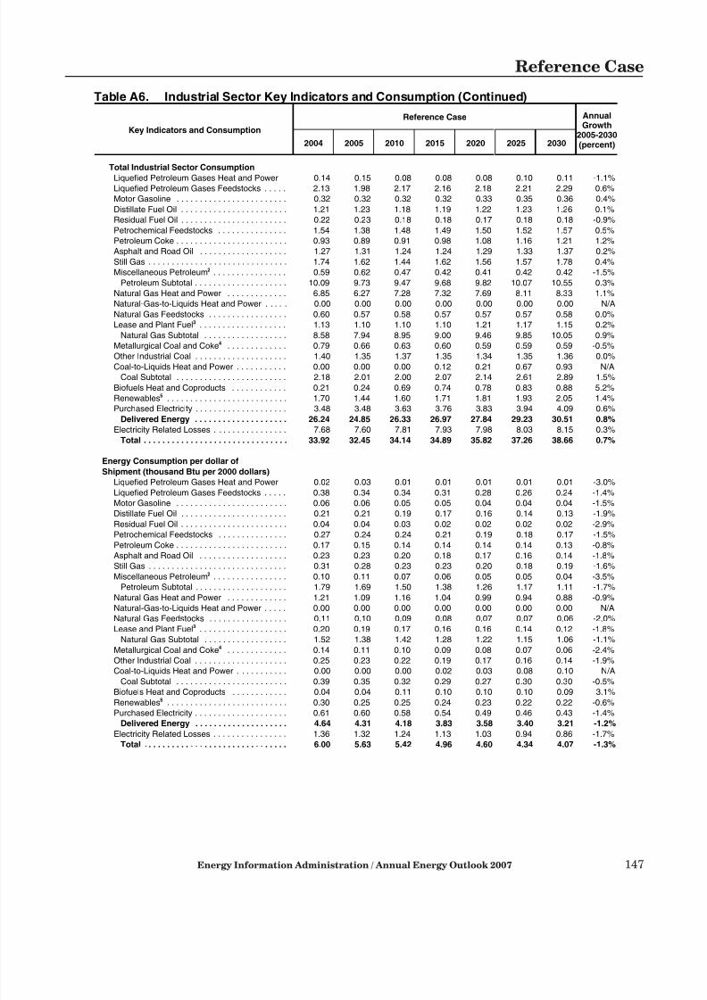
7/28/2019 2007 Annual Energy Outlook
http://slidepdf.com/reader/full/2007-annual-energy-outlook 156/243
Energy Information Administration / Annual Energy Outlook 2007 147
Reference Case
Table A6. Industrial Sector Key Indicators and Consumption (Continued)
Key Indicators and Consumption
Reference Case AnnualGrowth
2005-2030(percent)2004 2005 2010 2015 2020 2025 2030
Total Industrial Sector Consumption
Liquefied Petroleum Gases Heat and Power 0.14 0.15 0.08 0.08 0.08 0.10 0.11 -1.1%Liquefied Petroleum Gases Feedstocks . . . . . 2.13 1.98 2.17 2.16 2.18 2.21 2.29 0.6%
Motor Gasoline . . . . . . . . . . . . . . . . . . . . . . . . 0.32 0.32 0.32 0.32 0.33 0.35 0.36 0.4%
Distillate Fuel Oil . . . . . . . . . . . . . . . . . . . . . . . 1.21 1.23 1.18 1.19 1.22 1.23 1.26 0.1%
Residual Fuel Oil . . . . . . . . . . . . . . . . . . . . . . . 0.22 0.23 0.18 0.18 0.17 0.18 0.18 -0.9%
Petrochemical Feedstocks . . . . . . . . . . . . . . . 1.54 1.38 1.48 1.49 1.50 1.52 1.57 0.5%
Petroleum Coke . . . . . . . . . . . . . . . . . . . . . . . . 0.93 0.89 0.91 0.98 1.08 1.16 1.21 1.2%
Asphalt and Road Oil . . . . . . . . . . . . . . . . . . . 1.27 1.31 1.24 1.24 1.29 1.33 1.37 0.2%
Still Gas . . . . . . . . . . . . . . . . . . . . . . . . . . . . . . 1.74 1.62 1.44 1.62 1.56 1.57 1.78 0.4%
Miscellaneous Petroleum2 . . . . . . . . . . . . . . . . 0.59 0.62 0.47 0.42 0.41 0.42 0.42 -1.5%
Petroleum Subtotal . . . . . . . . . . . . . . . . . . . . 10.09 9.73 9.47 9.68 9.82 10.07 10.55 0.3%
Natural Gas Heat and Power . . . . . . . . . . . . . 6.85 6.27 7.28 7.32 7.69 8.11 8.33 1.1%
Natural-Gas-to-Liquids Heat and Power . . . . . 0.00 0.00 0.00 0.00 0.00 0.00 0.00 N/A
Natural Gas Feedstocks . . . . . . . . . . . . . . . . . 0.60 0.57 0.58 0.57 0.57 0.57 0.58 0.0%
Lease and Plant Fuel3 . . . . . . . . . . . . . . . . . . . 1.13 1.10 1.10 1.10 1.21 1.17 1.15 0.2%
Natural Gas Subtotal . . . . . . . . . . . . . . . . . . 8.58 7.94 8.95 9.00 9.46 9.85 10.05 0.9%
Metallurgical Coal and Coke4 . . . . . . . . . . . . . 0.79 0.66 0.63 0.60 0.59 0.59 0.59 -0.5%
Other Industrial Coal . . . . . . . . . . . . . . . . . . . . 1.40 1.35 1.37 1.35 1.34 1.35 1.36 0.0%
Coal-to-Liquids Heat and Power . . . . . . . . . . . 0.00 0.00 0.00 0.12 0.21 0.67 0.93 N/A
Coal Subtotal . . . . . . . . . . . . . . . . . . . . . . . . 2.18 2.01 2.00 2.07 2.14 2.61 2.89 1.5%
Biofuels Heat and Coproducts . . . . . . . . . . . . 0.21 0.24 0.69 0.74 0.78 0.83 0.88 5.2%
Renewables5 . . . . . . . . . . . . . . . . . . . . . . . . . . 1.70 1.44 1.60 1.71 1.81 1.93 2.05 1.4%
Purchased Electricity . . . . . . . . . . . . . . . . . . . . 3.48 3.48 3.63 3.76 3.83 3.94 4.09 0.6%
Delivered Energy . . . . . . . . . . . . . . . . . . . . 26.24 24.85 26.33 26.97 27.84 29.23 30.51 0.8%
Electricity Related Losses . . . . . . . . . . . . . . . . 7.68 7.60 7.81 7.93 7.98 8.03 8.15 0.3%
Total . . . . . . . . . . . . . . . . . . . . . . . . . . . . . . . 33.92 32.45 34.14 34.89 35.82 37.26 38.66 0.7%
Energy Consumption per dollar of
Shipment (thousand Btu per 2000 dollars)
Liquefied Petroleum Gases Heat and Power 0.02 0.03 0.01 0.01 0.01 0.01 0.01 -3.0%
Liquefied Petroleum Gases Feedstocks . . . . . 0.38 0.34 0.34 0.31 0.28 0.26 0.24 -1.4%
Motor Gasoline . . . . . . . . . . . . . . . . . . . . . . . . 0.06 0.06 0.05 0.05 0.04 0.04 0.04 -1.5%
Distillate Fuel Oil . . . . . . . . . . . . . . . . . . . . . . . 0.21 0.21 0.19 0.17 0.16 0.14 0.13 -1.9%
Residual Fuel Oil . . . . . . . . . . . . . . . . . . . . . . . 0.04 0.04 0.03 0.02 0.02 0.02 0.02 -2.9%Petrochemical Feedstocks . . . . . . . . . . . . . . . 0.27 0.24 0.24 0.21 0.19 0.18 0.17 -1.5%
Petroleum Coke . . . . . . . . . . . . . . . . . . . . . . . . 0.17 0.15 0.14 0.14 0.14 0.14 0.13 -0.8%
Asphalt and Road Oil . . . . . . . . . . . . . . . . . . . 0.23 0.23 0.20 0.18 0.17 0.16 0.14 -1.8%
Still Gas . . . . . . . . . . . . . . . . . . . . . . . . . . . . . . 0.31 0.28 0.23 0.23 0.20 0.18 0.19 -1.6%
Miscellaneous Petroleum2 . . . . . . . . . . . . . . . . 0.10 0.11 0.07 0.06 0.05 0.05 0.04 -3.5%
Petroleum Subtotal . . . . . . . . . . . . . . . . . . . . 1.79 1.69 1.50 1.38 1.26 1.17 1.11 -1.7%
Natural Gas Heat and Power . . . . . . . . . . . . . 1.21 1.09 1.16 1.04 0.99 0.94 0.88 -0.9%
Natural-Gas-to-Liquids Heat and Power . . . . . 0.00 0.00 0.00 0.00 0.00 0.00 0.00 N/A
Natural Gas Feedstocks . . . . . . . . . . . . . . . . . 0.11 0.10 0.09 0.08 0.07 0.07 0.06 -2.0%
Lease and Plant Fuel3 . . . . . . . . . . . . . . . . . . . 0.20 0.19 0.17 0.16 0.16 0.14 0.12 -1.8%
Natural Gas Subtotal . . . . . . . . . . . . . . . . . . 1.52 1.38 1.42 1.28 1.22 1.15 1.06 -1.1%
Metallurgical Coal and Coke4 . . . . . . . . . . . . . 0.14 0.11 0.10 0.09 0.08 0.07 0.06 -2.4%
Other Industrial Coal . . . . . . . . . . . . . . . . . . . . 0.25 0.23 0.22 0.19 0.17 0.16 0.14 -1.9%
Coal-to-Liquids Heat and Power . . . . . . . . . . . 0.00 0.00 0.00 0.02 0.03 0.08 0.10 N/A
Coal Subtotal . . . . . . . . . . . . . . . . . . . . . . . . 0.39 0.35 0.32 0.29 0.27 0.30 0.30 -0.5%
Biofuels Heat and Coproducts . . . . . . . . . . . . 0.04 0.04 0.11 0.10 0.10 0.10 0.09 3.1%
Renewables5 . . . . . . . . . . . . . . . . . . . . . . . . . . 0.30 0.25 0.25 0.24 0.23 0.22 0.22 -0.6%Purchased Electricity . . . . . . . . . . . . . . . . . . . . 0.61 0.60 0.58 0.54 0.49 0.46 0.43 -1.4%
Delivered Energy . . . . . . . . . . . . . . . . . . . . 4.64 4.31 4.18 3.83 3.58 3.40 3.21 -1.2%
Electricity Related Losses . . . . . . . . . . . . . . . . 1.36 1.32 1.24 1.13 1.03 0.94 0.86 -1.7%
Total . . . . . . . . . . . . . . . . . . . . . . . . . . . . . . . 6.00 5.63 5.42 4.96 4.60 4.34 4.07 -1.3%

7/28/2019 2007 Annual Energy Outlook
http://slidepdf.com/reader/full/2007-annual-energy-outlook 157/243
148 Energy Information Administration / Annual Energy Outlook 2007
Reference Case
Table A6. Industrial Sector Key Indicators and Consumption (Continued)
Key Indicators and Consumption
Reference Case AnnualGrowth
2005-2030(percent)2004 2005 2010 2015 2020 2025 2030
Industrial Combined Heat and Power
Capacity (gigawatts) . . . . . . . . . . . . . . . . . . . . . 26.31 25.53 29.28 34.19 39.05 48.82 56.54 3.2%Generation (billion kilowatthours) . . . . . . . . . . . 153.21 143.13 169.93 206.73 243.02 317.63 375.86 3.9%
1Includes energy for combined heat and power plants, except those whose primary business is to sell electricity, or electricity and heat, to the public.2Includes lubricants and miscellaneous petroleum products.3Represents natural gas used in well, field, and lease operations, and in natural gas processing plant machinery.4Includes net coal coke imports.5Includes consumption of energy produced from hydroelectric, wood and wood waste, municipal solid waste, and other biomass sources.Btu = British thermal unit.N/A = Not applicable.Note: Totals may not equal sum of components due to independent rounding. Data for 2004 and 2005 are model results and may differ slightly from official EIA
data reports.Sources: 2004 and 2005 prices for motor gasoline and distillate fuel oil are based on: Energy Information Administration (EIA), Petroleum Marketing Annual
2005 , DOE/EIA-0487(2005) (Washington, DC, August 2006). 2004 and 2005 coal prices are based on: EIA, Quarterly Coal Report, October-December 2005 ,DOE/EIA-0121(2005/4Q) (Washington, DC, March 2006) and EIA, AEO2007 National Energy Modeling System run AEO2007.D112106A. 2004 and 2005electricity prices: EIA, Annual Energy Review 2005 , DOE/EIA-0384(2005) (Washington, DC, July 2006). 2004 and 2005 natural gas prices are based on: EIA,Manufacturing Energy Consumption Survey 1994 and industrial and wellhead prices from the Natural Gas Annual 2004 , DOE/EIA-0131(2004) (Washington, DC,December 2005) and the Natural Gas Monthly , DOE/EIA-0130(2006/04) (Washington, DC, April 2006). 2004 refining consumption based on: Petroleum Supply Annual 2004, DOE/EIA-0340(2004)/1 (Washington, DC, June 2005). 2005 refining consumption based on: Petroleum Supply Annual 2005,DOE/EIA-0340(2005)/1 (Washington, DC, October 2006). Other 2004 and 2005 consumption values are based on: EIA, Annual Energy Review 2005 , DOE/EIA-0384(2005) (Washington, DC, July 2006). 2004 and 2005 shipments: Global Insight industry model, July 2006. Projections: EIA, AEO2007 National EnergyModeling System run AEO2007.D112106A.

7/28/2019 2007 Annual Energy Outlook
http://slidepdf.com/reader/full/2007-annual-energy-outlook 158/243
Energy Information Administration / Annual Energy Outlook 2007 149
Reference Case
Table A7. Transportation Sector Key Indicators and Delivered Energy Consumption
Key Indicators and Consumption
Reference Case AnnualGrowth
2005-2030(percent)2004 2005 2010 2015 2020 2025 2030
Key Indicators
Travel Indicators
(billion vehicle miles traveled)
Light-Duty Vehicles less than 8,500 pounds 2652 2655 2799 3125 3474 3839 4226 1.9%
Commercial Light Trucks1 . . . . . . . . . . . . . . 66 67 72 81 89 99 110 2.0%
Freight Trucks greater than 10,000 pounds 226 230 255 287 318 355 397 2.2%
(billion seat miles available)
Air . . . . . . . . . . . . . . . . . . . . . . . . . . . . . . . . 992 1027 1172 1302 1410 1478 1544 1.6%
(billion ton miles traveled)
Rail . . . . . . . . . . . . . . . . . . . . . . . . . . . . . . . 1590 1590 1714 1864 2000 2223 2445 1.7%
Domestic Shipping . . . . . . . . . . . . . . . . . . . 618 613 661 699 730 751 775 0.9%
Energy Efficiency Indicators
(miles per gallon)
New Light-Duty Vehicle2 . . . . . . . . . . . . . . . 24.6 25.2 27.3 27.9 28.2 28.9 29.2 0.6%
New Car2 . . . . . . . . . . . . . . . . . . . . . . . . . 29.1 30.0 31.7 32.4 32.8 33.4 33.7 0.5%
New Light Truck2 . . . . . . . . . . . . . . . . . . . 21.5 21.8 23.7 24.7 25.3 26.1 26.5 0.8%
Light-Duty Stock
3
. . . . . . . . . . . . . . . . . . . . . 19.6 19.6 19.8 20.6 21.2 21.8 22.2 0.5%New Commercial Light Truck1 . . . . . . . . . . . 14.5 14.6 15.8 16.4 16.7 17.2 17.4 0.7%
Stock Commercial Light Truck1 . . . . . . . . . . 14.0 14.1 14.7 15.5 16.2 16.7 17.0 0.8%
Freight Truck . . . . . . . . . . . . . . . . . . . . . . . . 6.0 6.0 6.0 6.2 6.4 6.6 6.7 0.4%
(seat miles per gallon)
Aircraft . . . . . . . . . . . . . . . . . . . . . . . . . . . . . 55.5 55.7 58.2 61.9 66.4 71.6 75.6 1.2%
(ton miles per thousand Btu)
Rail . . . . . . . . . . . . . . . . . . . . . . . . . . . . . . . 2.9 2.9 2.9 2.9 3.0 3.0 3.0 0.1%
Domestic Shipping . . . . . . . . . . . . . . . . . . . 2.4 2.4 2.4 2.4 2.4 2.5 2.5 0.1%
Energy Use by Mode
(quadrillion Btu)
Light-Duty Vehicles . . . . . . . . . . . . . . . . . . . . . . 16.34 16.36 16.76 17.99 19.44 20.98 22.66 1.3%
Commercial Light Trucks1 . . . . . . . . . . . . . . . . . 0.59 0.59 0.61 0.65 0.69 0.75 0.81 1.3%
Bus Transportation . . . . . . . . . . . . . . . . . . . . . . 0.26 0.26 0.27 0.28 0.28 0.29 0.30 0.5%
Freight Trucks . . . . . . . . . . . . . . . . . . . . . . . . . . 4.70 4.77 5.29 5.80 6.18 6.71 7.40 1.8%
Rail, Passenger . . . . . . . . . . . . . . . . . . . . . . . . . 0.04 0.04 0.05 0.05 0.05 0.05 0.06 1.1%
Rail, Freight . . . . . . . . . . . . . . . . . . . . . . . . . . . . 0.55 0.55 0.59 0.63 0.68 0.75 0.82 1.6%Shipping, Domestic . . . . . . . . . . . . . . . . . . . . . . 0.26 0.26 0.27 0.29 0.30 0.31 0.32 0.9%
Shipping, International . . . . . . . . . . . . . . . . . . . 0.69 0.76 0.77 0.78 0.79 0.80 0.80 0.2%
Recreational Boats . . . . . . . . . . . . . . . . . . . . . . 0.19 0.18 0.20 0.23 0.24 0.25 0.27 1.5%
Air . . . . . . . . . . . . . . . . . . . . . . . . . . . . . . . . . . . 2.85 2.84 3.50 3.79 3.97 4.00 4.11 1.5%
Military Use . . . . . . . . . . . . . . . . . . . . . . . . . . . . 0.71 0.71 0.73 0.75 0.77 0.79 0.80 0.5%
Lubricants . . . . . . . . . . . . . . . . . . . . . . . . . . . . . 0.15 0.15 0.15 0.15 0.16 0.16 0.16 0.4%
Pipeline Fuel . . . . . . . . . . . . . . . . . . . . . . . . . . . 0.59 0.58 0.66 0.70 0.79 0.79 0.79 1.3%
Total . . . . . . . . . . . . . . . . . . . . . . . . . . . . . . . . 27.92 28.05 29.86 32.07 34.33 36.63 39.29 1.4%

7/28/2019 2007 Annual Energy Outlook
http://slidepdf.com/reader/full/2007-annual-energy-outlook 159/243
150 Energy Information Administration / Annual Energy Outlook 2007
Reference Case
Table A7. Transportation Sector Key Indicators and Delivered Energy Consumption(Continued)
Key Indicators and Consumption
Reference Case AnnualGrowth
2005-2030(percent)2004 2005 2010 2015 2020 2025 2030
Energy Use by Mode
(million barrels per day oil equivalent)
Light-Duty Vehicles . . . . . . . . . . . . . . . . . . . . . . 8.57 8.58 9.00 9.66 10.43 11.25 12.15 1.4%
Commercial Light Trucks1 . . . . . . . . . . . . . . . . . 0.31 0.31 0.33 0.35 0.37 0.40 0.44 1.4%
Bus Transportation . . . . . . . . . . . . . . . . . . . . . . 0.13 0.13 0.13 0.13 0.14 0.14 0.14 0.6%
Freight Trucks . . . . . . . . . . . . . . . . . . . . . . . . . . 2.24 2.27 2.53 2.78 2.96 3.21 3.54 1.8%
Rail, Passenger . . . . . . . . . . . . . . . . . . . . . . . . . 0.02 0.02 0.02 0.02 0.02 0.03 0.03 1.1%
Rail, Freight . . . . . . . . . . . . . . . . . . . . . . . . . . . . 0.26 0.26 0.28 0.30 0.32 0.36 0.39 1.7%
Shipping, Domestic . . . . . . . . . . . . . . . . . . . . . . 0.12 0.12 0.13 0.13 0.14 0.14 0.15 0.9%
Shipping, International . . . . . . . . . . . . . . . . . . . 0.30 0.33 0.34 0.34 0.35 0.35 0.35 0.2%
Recreational Boats . . . . . . . . . . . . . . . . . . . . . . 0.10 0.10 0.11 0.12 0.13 0.14 0.15 1.6%
Air . . . . . . . . . . . . . . . . . . . . . . . . . . . . . . . . . . . 1.38 1.37 1.69 1.83 1.92 1.94 1.99 1.5%
Military Use . . . . . . . . . . . . . . . . . . . . . . . . . . . . 0.34 0.34 0.35 0.36 0.37 0.38 0.38 0.5%
Lubricants . . . . . . . . . . . . . . . . . . . . . . . . . . . . . 0.07 0.07 0.07 0.07 0.07 0.08 0.08 0.4%
Pipeline Fuel . . . . . . . . . . . . . . . . . . . . . . . . . . . 0.30 0.29 0.33 0.35 0.40 0.40 0.40 1.3%
Total . . . . . . . . . . . . . . . . . . . . . . . . . . . . . . . . 14.14 14.19 15.31 16.45 17.62 18.81 20.18 1.4%
1Commercial trucks 8,500 to 10,000 pounds.2Environmental Protection Agency rated miles per gallon.3Combined car and light truck “on-the-road” estimate.Btu = British thermal unit.Note: Totals may not equal sum of components due to independent rounding. Data for 2004 and 2005 are model results and may differ slightly from official EIA
data reports.Sources: 2004 and 2005: Energy Information Administration (EIA), Natural Gas Annual 2004 , DOE/EIA-0131(2004) (Washington, DC, December 2005); EIA,
Annual Energy Review 2005 , DOE/EIA-0384(2005) (Washington, DC, July 2006); Federal Highway Administration, Highway Statistics 2004 (Washington, DC,October 2005); Oak Ridge National Laboratory, Transportation Energy Data Book: Edition 25 and Annual (Oak Ridge, TN, 2005); National Highway Traffic andSafety Administration, Summary of Fuel Economy Performance (Washington, DC, March 2004); U.S. Department of Commerce, Bureau of the Census, “VehicleInventory and Use Survey,” EC97TV (Washington, DC, October 1999); EIA, State Energy Data Report 2002 , DOE/EIA-0214(2002) (Washington, DC, December2005); EIA, Estimated Number of Alternative-Fueled Vehicles , http://www.eia.doe.gov/cneaf/alternate/page/datatables/aft1-13_03.html; U.S. Department ofTransportation, Research and Special Programs Administration, Air Carrier Statistics Monthly, December 2005/2004 (Washington, DC, 2005); EIA, Fuel Oil and Kerosene Sales 2004 , DOE/EIA-0535(2004) (Washington, DC, November 2005); and United States Department of Defense, Defense Fuel Supply Center.Projections: EIA, AEO2007 National Energy Modeling System run AEO2007.D112106A.

7/28/2019 2007 Annual Energy Outlook
http://slidepdf.com/reader/full/2007-annual-energy-outlook 160/243
Energy Information Administration / Annual Energy Outlook 2007 151
Reference Case
Table A8. Electricity Supply, Disposition, Prices, and Emissions(Billion Kilowatthours, Unless Otherwise Noted)
Supply, Disposition, and Prices
Reference Case AnnualGrowth
2005-2030(percent)2004 2005 2010 2015 2020 2025 2030
Generation by Fuel Type
Electric Power Sector1
Power Only2
Coal . . . . . . . . . . . . . . . . . . . . . . . . . . . . . . . . 1921 1956 2090 2233 2418 2766 3191 2.0%
Petroleum . . . . . . . . . . . . . . . . . . . . . . . . . . . . 111 111 82 89 89 91 92 -0.7%
Natural Gas3 . . . . . . . . . . . . . . . . . . . . . . . . . . 491 546 658 756 776 702 609 0.4%
Nuclear Power . . . . . . . . . . . . . . . . . . . . . . . . 789 780 789 812 885 886 896 0.6%
Pumped Storage/Other . . . . . . . . . . . . . . . . . -8 -7 -9 -9 -9 -9 -9 1.1%
Renewable Sources4 . . . . . . . . . . . . . . . . . . . 321 319 426 440 445 458 461 1.5%
Distributed Generation (Natural Gas) . . . . . . . 0 0 0 0 1 2 5 N/A
Total . . . . . . . . . . . . . . . . . . . . . . . . . . . . . . 3624 3705 4037 4322 4605 4897 5245 1.4%
Combined Heat and Power5
Coal . . . . . . . . . . . . . . . . . . . . . . . . . . . . . . . . 36 37 31 29 29 29 29 -1.0%
Petroleum . . . . . . . . . . . . . . . . . . . . . . . . . . . . 5 5 1 1 1 1 1 -5.3%
Natural Gas . . . . . . . . . . . . . . . . . . . . . . . . . . 137 129 137 145 142 132 123 -0.2%
Renewable Sources . . . . . . . . . . . . . . . . . . . . 4 4 4 3 3 3 4 0.1%
Total . . . . . . . . . . . . . . . . . . . . . . . . . . . . . . 185 178 172 179 176 166 157 -0.5%Total Net Generation . . . . . . . . . . . . . . . . . . . . 3808 3883 4209 4501 4781 5063 5402 1.3%
Less Direct Use . . . . . . . . . . . . . . . . . . . . . . . . . 35 35 34 34 34 34 34 -0.1%
Net Available to the Grid . . . . . . . . . . . . . . . . . . 3773 3849 4175 4467 4747 5029 5368 1.3%
End-Use Generation6
Coal . . . . . . . . . . . . . . . . . . . . . . . . . . . . . . . . . 22 22 22 33 41 85 110 6.6%
Petroleum . . . . . . . . . . . . . . . . . . . . . . . . . . . . . 6 6 11 13 13 13 14 3.4%
Natural Gas . . . . . . . . . . . . . . . . . . . . . . . . . . . 82 77 97 117 142 169 200 3.9%
Other Gaseous Fuels7 . . . . . . . . . . . . . . . . . . . 6 5 4 5 5 5 6 0.8%
Renewable Sources4 . . . . . . . . . . . . . . . . . . . . 37 34 37 40 44 48 54 1.9%
Other8 . . . . . . . . . . . . . . . . . . . . . . . . . . . . . . . . 14 12 11 11 11 11 11 -0.0%
Total . . . . . . . . . . . . . . . . . . . . . . . . . . . . . . . 167 155 183 220 256 332 395 3.8%
Less Direct Use . . . . . . . . . . . . . . . . . . . . . . . . 136 126 144 168 194 236 276 3.2%
Total Sales to the Grid . . . . . . . . . . . . . . . . 31 29 39 51 62 96 119 5.9%
Total Electricity Generation . . . . . . . . . . . . . . . . . 3975 4038 4392 4721 5037 5395 5797 1.5%Total Net Generation to the Grid . . . . . . . . . . . . . 3804 3877 4214 4519 4810 5125 5487 1.4%
Net Imports . . . . . . . . . . . . . . . . . . . . . . . . . . . . . . 11 25 11 8 11 13 13 -2.6%
Electricity Sales by Sector
Residential . . . . . . . . . . . . . . . . . . . . . . . . . . . . . . 1294 1365 1483 1591 1701 1797 1896 1.3%
Commercial . . . . . . . . . . . . . . . . . . . . . . . . . . . . . 1229 1267 1398 1548 1694 1864 2062 2.0%
Industrial . . . . . . . . . . . . . . . . . . . . . . . . . . . . . . . 1018 1021 1063 1103 1123 1155 1199 0.6%
Transportation . . . . . . . . . . . . . . . . . . . . . . . . . . . 7 7 8 9 10 11 12 1.8%
Total . . . . . . . . . . . . . . . . . . . . . . . . . . . . . . . . . 3548 3660 3953 4251 4528 4827 5168 1.4%
Direct Use . . . . . . . . . . . . . . . . . . . . . . . . . . . . . . 171 161 178 202 228 270 310 2.6%
Total Electricity Use . . . . . . . . . . . . . . . . . . . . 3719 3821 4132 4453 4756 5097 5478 1.5%
End-Use Prices
(2005 cents per kilowatthour)
Residential . . . . . . . . . . . . . . . . . . . . . . . . . . . . . . 9.2 9.4 9.2 8.9 9.0 9.1 9.1 -0.1%
Commercial . . . . . . . . . . . . . . . . . . . . . . . . . . . . . 8.4 8.6 8.4 8.0 8.2 8.3 8.3 -0.2%
Industrial . . . . . . . . . . . . . . . . . . . . . . . . . . . . . . . 5.4 5.7 6.1 5.6 5.8 5.9 5.9 0.2%
Transportation . . . . . . . . . . . . . . . . . . . . . . . . . . . 8.9 8.6 8.5 8.1 8.3 8.3 8.3 -0.1%
All Sectors Average . . . . . . . . . . . . . . . . . . . . 7.9 8.1 8.1 7.7 7.9 8.0 8.1 -0.0%
Prices by Service Category
(2005 cents per kilowatthour)
Generation . . . . . . . . . . . . . . . . . . . . . . . . . . . . . . 5.2 5.4 5.4 5.0 5.2 5.4 5.4 0.0%
Transmission . . . . . . . . . . . . . . . . . . . . . . . . . . . . 0.6 0.6 0.6 0.7 0.7 0.7 0.7 1.0%
Distribution . . . . . . . . . . . . . . . . . . . . . . . . . . . . . 2.1 2.1 2.1 2.1 2.0 2.0 1.9 -0.3%

7/28/2019 2007 Annual Energy Outlook
http://slidepdf.com/reader/full/2007-annual-energy-outlook 161/243
152 Energy Information Administration / Annual Energy Outlook 2007
Reference Case
Table A8. Electricity Supply, Disposition, Prices, and Emissions (Continued)(Billion Kilowatthours, Unless Otherwise Noted)
Supply, Disposition, and Prices
Reference Case AnnualGrowth
2005-2030(percent)2004 2005 2010 2015 2020 2025 2030
Electric Power Sector Emissions1
Sulfur Dioxide (million tons) . . . . . . . . . . . . . . . . 10.26 10.21 6.56 4.46 3.90 3.68 3.63 -4.1%
Nitrogen Oxide (million tons) . . . . . . . . . . . . . . . . 3.75 3.60 2.41 2.20 2.22 2.25 2.28 -1.8%
Mercury (tons) . . . . . . . . . . . . . . . . . . . . . . . . . . . 47.15 51.25 37.21 24.64 19.24 16.86 15.48 -4.7%
1Includes electricity-only and combined heat and power plants whose primary business is to sell electricity, or electricity and heat, to the public.2Includes plants that only produce electricity.3Includes electricity generation from fuel cells.4Includes conventional hydroelectric, geothermal, wood, wood waste, municipal solid waste, landfill gas, other biomass, solar, and wind power.5Includes combined heat and power plants whose primary business is to sell electricity and heat to the public (i.e., those that report North American Industry
Classification System code 22).6Includes combined heat and power plants and electricity-only plants in the commercial and industrial sectors; and small on-site generating systems in the
residential, commercial, and industrial sectors used primarily for own-use generation, but which may also sell some power to the grid.7Includes refinery gas and still gas.8Includes batteries, chemicals, hydrogen, pitch, purchased steam, sulfur, and miscellaneous technologies.N/A = Not applicable.Note: Totals may not equal sum of components due to independent rounding. Data for 2004 and 2005 are model results and may differ slightly from official EIA
data reports.Sources: 2004 and 2005 electric power sector generation; sales to utilities; net imports; electricity sales; and emissions: Energy Information Administration
(EIA), Annual Energy Review 2005 , DOE/EIA-0384(2005) (Washington, DC, July 2006), and supporting databases. 2004 and 2005 prices: EIA, AEO2007National Energy Modeling System run AEO2007.D112106A. Projections: EIA, AEO2007 National Energy Modeling System run AEO2007.D112106A.
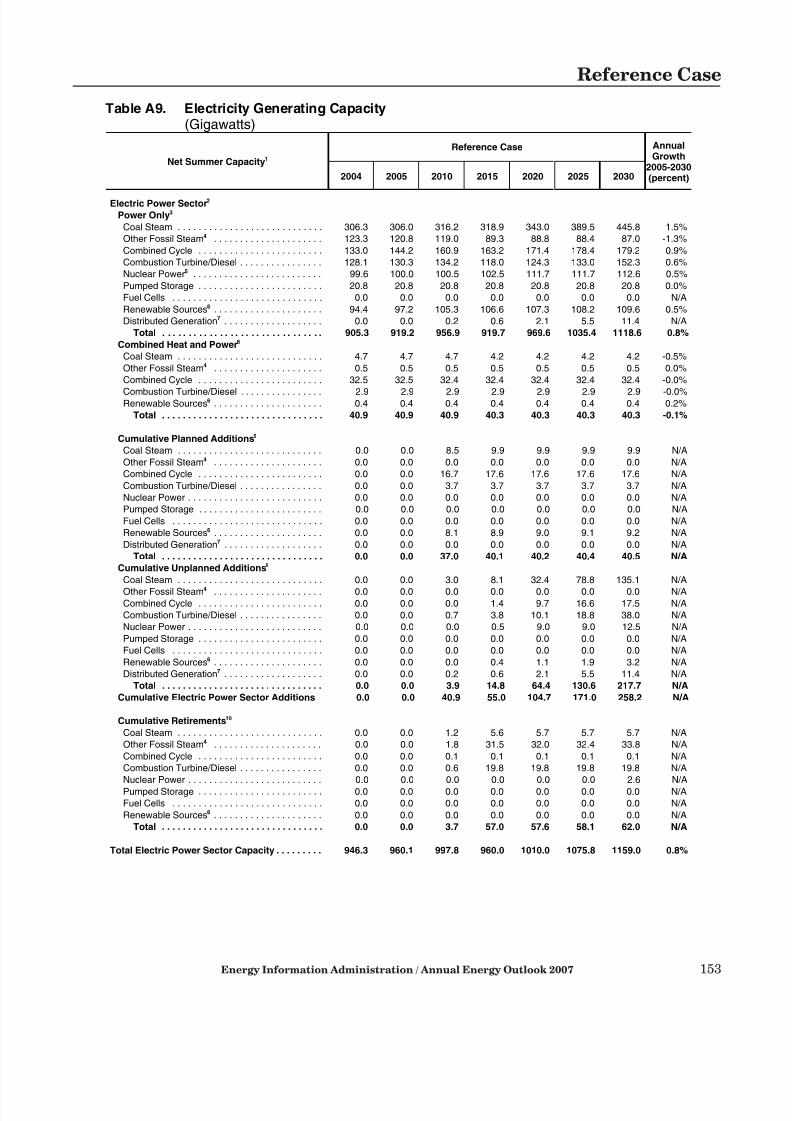
7/28/2019 2007 Annual Energy Outlook
http://slidepdf.com/reader/full/2007-annual-energy-outlook 162/243
Energy Information Administration / Annual Energy Outlook 2007 153
Reference Case
Table A9. Electricity Generating Capacity(Gigawatts)
Net Summer Capacity1
Reference Case AnnualGrowth
2005-2030(percent)2004 2005 2010 2015 2020 2025 2030
Electric Power Sector2
Power Only3
Coal Steam . . . . . . . . . . . . . . . . . . . . . . . . . . . . 306.3 306.0 316.2 318.9 343.0 389.5 445.8 1.5%
Other Fossil Steam4 . . . . . . . . . . . . . . . . . . . . . 123.3 120.8 119.0 89.3 88.8 88.4 87.0 -1.3%
Combined Cycle . . . . . . . . . . . . . . . . . . . . . . . . 133.0 144.2 160.9 163.2 171.4 178.4 179.2 0.9%
Combustion Turbine/Diesel . . . . . . . . . . . . . . . . 128.1 130.3 134.2 118.0 124.3 133.0 152.3 0.6%
Nuclear Power5 . . . . . . . . . . . . . . . . . . . . . . . . . 99.6 100.0 100.5 102.5 111.7 111.7 112.6 0.5%
Pumped Storage . . . . . . . . . . . . . . . . . . . . . . . . 20.8 20.8 20.8 20.8 20.8 20.8 20.8 0.0%
Fuel Cells . . . . . . . . . . . . . . . . . . . . . . . . . . . . . 0.0 0.0 0.0 0.0 0.0 0.0 0.0 N/A
Renewable Sources6 . . . . . . . . . . . . . . . . . . . . . 94.4 97.2 105.3 106.6 107.3 108.2 109.6 0.5%
Distributed Generation7 . . . . . . . . . . . . . . . . . . . 0.0 0.0 0.2 0.6 2.1 5.5 11.4 N/A
Total . . . . . . . . . . . . . . . . . . . . . . . . . . . . . . . 905.3 919.2 956.9 919.7 969.6 1035.4 1118.6 0.8%
Combined Heat and Power8
Coal Steam . . . . . . . . . . . . . . . . . . . . . . . . . . . . 4.7 4.7 4.7 4.2 4.2 4.2 4.2 -0.5%
Other Fossil Steam4 . . . . . . . . . . . . . . . . . . . . . 0.5 0.5 0.5 0.5 0.5 0.5 0.5 0.0%
Combined Cycle . . . . . . . . . . . . . . . . . . . . . . . . 32.5 32.5 32.4 32.4 32.4 32.4 32.4 -0.0%
Combustion Turbine/Diesel . . . . . . . . . . . . . . . . 2.9 2.9 2.9 2.9 2.9 2.9 2.9 -0.0%Renewable Sources6 . . . . . . . . . . . . . . . . . . . . . 0.4 0.4 0.4 0.4 0.4 0.4 0.4 0.2%
Total . . . . . . . . . . . . . . . . . . . . . . . . . . . . . . . 40.9 40.9 40.9 40.3 40.3 40.3 40.3 -0.1%
Cumulative Planned Additions9
Coal Steam . . . . . . . . . . . . . . . . . . . . . . . . . . . . 0.0 0.0 8.5 9.9 9.9 9.9 9.9 N/A
Other Fossil Steam4 . . . . . . . . . . . . . . . . . . . . . 0.0 0.0 0.0 0.0 0.0 0.0 0.0 N/A
Combined Cycle . . . . . . . . . . . . . . . . . . . . . . . . 0.0 0.0 16.7 17.6 17.6 17.6 17.6 N/A
Combustion Turbine/Diesel . . . . . . . . . . . . . . . . 0.0 0.0 3.7 3.7 3.7 3.7 3.7 N/A
Nuclear Power . . . . . . . . . . . . . . . . . . . . . . . . . . 0.0 0.0 0.0 0.0 0.0 0.0 0.0 N/A
Pumped Storage . . . . . . . . . . . . . . . . . . . . . . . . 0.0 0.0 0.0 0.0 0.0 0.0 0.0 N/A
Fuel Cells . . . . . . . . . . . . . . . . . . . . . . . . . . . . . 0.0 0.0 0.0 0.0 0.0 0.0 0.0 N/A
Renewable Sources6 . . . . . . . . . . . . . . . . . . . . . 0.0 0.0 8.1 8.9 9.0 9.1 9.2 N/A
Distributed Generation7 . . . . . . . . . . . . . . . . . . . 0.0 0.0 0.0 0.0 0.0 0.0 0.0 N/A
Total . . . . . . . . . . . . . . . . . . . . . . . . . . . . . . . 0.0 0.0 37.0 40.1 40.2 40.4 40.5 N/A
Cumulative Unplanned Additions9
Coal Steam . . . . . . . . . . . . . . . . . . . . . . . . . . . . 0.0 0.0 3.0 8.1 32.4 78.8 135.1 N/A
Other Fossil Steam4 . . . . . . . . . . . . . . . . . . . . . 0.0 0.0 0.0 0.0 0.0 0.0 0.0 N/ACombined Cycle . . . . . . . . . . . . . . . . . . . . . . . . 0.0 0.0 0.0 1.4 9.7 16.6 17.5 N/A
Combustion Turbine/Diesel . . . . . . . . . . . . . . . . 0.0 0.0 0.7 3.8 10.1 18.8 38.0 N/A
Nuclear Power . . . . . . . . . . . . . . . . . . . . . . . . . . 0.0 0.0 0.0 0.5 9.0 9.0 12.5 N/A
Pumped Storage . . . . . . . . . . . . . . . . . . . . . . . . 0.0 0.0 0.0 0.0 0.0 0.0 0.0 N/A
Fuel Cells . . . . . . . . . . . . . . . . . . . . . . . . . . . . . 0.0 0.0 0.0 0.0 0.0 0.0 0.0 N/A
Renewable Sources6 . . . . . . . . . . . . . . . . . . . . . 0.0 0.0 0.0 0.4 1.1 1.9 3.2 N/A
Distributed Generation7 . . . . . . . . . . . . . . . . . . . 0.0 0.0 0.2 0.6 2.1 5.5 11.4 N/A
Total . . . . . . . . . . . . . . . . . . . . . . . . . . . . . . . 0.0 0.0 3.9 14.8 64.4 130.6 217.7 N/A
Cumulative Electric Power Sector Additions 0.0 0.0 40.9 55.0 104.7 171.0 258.2 N/A
Cumulative Retirements10
Coal Steam . . . . . . . . . . . . . . . . . . . . . . . . . . . . 0.0 0.0 1.2 5.6 5.7 5.7 5.7 N/A
Other Fossil Steam4 . . . . . . . . . . . . . . . . . . . . . 0.0 0.0 1.8 31.5 32.0 32.4 33.8 N/A
Combined Cycle . . . . . . . . . . . . . . . . . . . . . . . . 0.0 0.0 0.1 0.1 0.1 0.1 0.1 N/A
Combustion Turbine/Diesel . . . . . . . . . . . . . . . . 0.0 0.0 0.6 19.8 19.8 19.8 19.8 N/A
Nuclear Power . . . . . . . . . . . . . . . . . . . . . . . . . . 0.0 0.0 0.0 0.0 0.0 0.0 2.6 N/A
Pumped Storage . . . . . . . . . . . . . . . . . . . . . . . . 0.0 0.0 0.0 0.0 0.0 0.0 0.0 N/A
Fuel Cells . . . . . . . . . . . . . . . . . . . . . . . . . . . . . 0.0 0.0 0.0 0.0 0.0 0.0 0.0 N/A
Renewable Sources6 . . . . . . . . . . . . . . . . . . . . . 0.0 0.0 0.0 0.0 0.0 0.0 0.0 N/A
Total . . . . . . . . . . . . . . . . . . . . . . . . . . . . . . . 0.0 0.0 3.7 57.0 57.6 58.1 62.0 N/A
Total Electric Power Sector Capacity . . . . . . . . . 946.3 960.1 997.8 960.0 1010.0 1075.8 1159.0 0.8%

7/28/2019 2007 Annual Energy Outlook
http://slidepdf.com/reader/full/2007-annual-energy-outlook 163/243
154 Energy Information Administration / Annual Energy Outlook 2007
Reference Case
Table A9. Electricity Generating Capacity (Continued)(Gigawatts)
Net Summer Capacity1
Reference Case AnnualGrowth
2005-2030(percent)2004 2005 2010 2015 2020 2025 2030
End-Use Generators11
Coal . . . . . . . . . . . . . . . . . . . . . . . . . . . . . . . . . . . 4.1 4.2 4.1 5.6 6.6 12.2 15.4 5.4%
Petroleum . . . . . . . . . . . . . . . . . . . . . . . . . . . . . . 1.6 1.6 1.6 1.8 1.8 1.9 1.9 0.7%
Natural Gas . . . . . . . . . . . . . . . . . . . . . . . . . . . . . 13.9 13.5 16.9 19.5 22.8 26.4 30.4 3.3%
Other Gaseous Fuels . . . . . . . . . . . . . . . . . . . . . 1.8 1.8 1.9 1.9 1.9 2.0 2.0 0.4%
Renewable Sources6 . . . . . . . . . . . . . . . . . . . . . . 5.8 5.6 6.4 7.0 7.7 8.7 10.7 2.6%
Other . . . . . . . . . . . . . . . . . . . . . . . . . . . . . . . . . . 1.1 0.8 0.8 0.8 0.8 0.8 0.8 0.0%
Total . . . . . . . . . . . . . . . . . . . . . . . . . . . . . . . . . 28.2 27.5 31.7 36.7 41.7 52.0 61.3 3.3%
Cumulative Capacity Additions9 0.0 0.0 4.2 9.2 14.2 24.5 33.8 N/A
1Net summer capacity is the steady hourly output that generating equipment is expected to supply to system load (exclusive of auxiliary power), asdemonstrated by tests during summer peak demand.
2Includes electricity-only and combined heat and power plants whose primary business is to sell electricity, or electricity and heat, to the public.3Includes plants that only produce electricity. Includes capacity increases (uprates) at existing units.4Includes oil-, gas-, and dual-fired capacity.5Nuclear capacity includes 2.7 gigawatts of uprates through 2030.6
Includes conventional hydroelectric, geothermal, wood, wood waste, municipal solid waste, landfill gas, other biomass, solar, and wind power. Facilities co-firing biomass and coal are classified as coal.7Primarily peak load capacity fueled by natural gas.8Includes combined heat and power plants whose primary business is to sell electricity and heat to the public (i.e., those that report North American Industry
Classification System code 22).9Cumulative additions after December 31, 2005.10Cumulative retirements after December 31, 2005.11Includes combined heat and power plants and electricity-only plants in the commercial and industrial sectors; and small on-site generating systems in the
residential, commercial, and industrial sectors used primarily for own-use generation, but which may also sell some power to the grid.N/A = Not applicable.Note: Totals may not equal sum of components due to independent rounding. Data for 2004 and 2005 are model results and may differ slightly from official EIA
data reports.Sources: 2004 and 2005 capacity and projected planned additions: Energy Information Administration (EIA), Form EIA-860, "Annual Electric Generator
Report” (preliminary). Projections: EIA, AEO2007 National Energy Modeling System run AEO2007.D112106A.

7/28/2019 2007 Annual Energy Outlook
http://slidepdf.com/reader/full/2007-annual-energy-outlook 164/243
Energy Information Administration / Annual Energy Outlook 2007 155
Reference Case
Table A10. Electricity Trade(Billion Kilowatthours, Unless Otherwise Noted)
Electricity Trade
Reference Case AnnualGrowth
2005-2030(percent)2004 2005 2010 2015 2020 2025 2030
Interregional Electricity Trade
Gross Domestic Sales
Firm Power . . . . . . . . . . . . . . . . . . . . . . . . . . . . . . 142.4 127.0 105.5 82.4 50.6 37.9 37.9 -4.7%
Economy . . . . . . . . . . . . . . . . . . . . . . . . . . . . . . . 118.3 180.5 178.6 181.7 167.6 164.1 149.9 -0.7%
Total . . . . . . . . . . . . . . . . . . . . . . . . . . . . . . . . . 260.7 307.5 284.0 264.1 218.2 201.9 187.7 -2.0%
Gross Domestic Sales (million 2005 dollars)
Firm Power . . . . . . . . . . . . . . . . . . . . . . . . . . . . . . 7675.9 6845.3 5684.4 4441.8 2727.5 2041.8 2041.8 -4.7%
Economy . . . . . . . . . . . . . . . . . . . . . . . . . . . . . . . 7058.7 11082.0 8729.7 7772.8 7568.7 7572.2 7117.4 -1.8%
Total . . . . . . . . . . . . . . . . . . . . . . . . . . . . . . . . . 14734.6 17927.2 14414.1 12214.6 10296.2 9613.9 9159.2 -2.7%
International Electricity Trade
Imports from Canada and Mexico
Firm Power . . . . . . . . . . . . . . . . . . . . . . . . . . . . . . 12.5 13.1 2.5 1.9 0.8 0.4 0.4 -13.2%
Economy . . . . . . . . . . . . . . . . . . . . . . . . . . . . . . . 21.7 31.4 26.7 23.9 25.9 26.0 26.1 -0.7%Total . . . . . . . . . . . . . . . . . . . . . . . . . . . . . . . . . 34.2 44.5 29.2 25.7 26.7 26.4 26.5 -2.1%
Exports to Canada and Mexico
Firm Power . . . . . . . . . . . . . . . . . . . . . . . . . . . . . . 7.4 2.9 1.0 0.7 0.2 0.0 0.0 N/A
Economy . . . . . . . . . . . . . . . . . . . . . . . . . . . . . . . 15.5 16.9 17.1 16.6 15.6 13.7 13.7 -0.8%
Total . . . . . . . . . . . . . . . . . . . . . . . . . . . . . . . . . 22.9 19.8 18.1 17.2 15.8 13.7 13.7 -1.5%
N/A = Not applicable.Note: Totals may not equal sum of components due to independent rounding. Data for 2004 and 2005 are model results and may differ slightly from official EIA
data reports. Firm Power Sales are capacity sales, meaning the delivery of the power is scheduled as part of the normal operating conditions of the affectedelectric systems. Economy Sales are subject to curtailment or cessation of delivery by the supplier in accordance with prior agreements or under specifiedconditions.
Sources: 2004 and 2005 interregional firm electricity trade data: North American Electric Reliability Council (NERC), Electricity Sales and Demand Database2004. 2004 and 2005 Mexican electricity trade data: Energy Information Administration (EIA), Electric Power Annual 2004 DOE/EIA-0348(2004) (Washington, DC,November 2005). 2004 Canadian international electricity trade data: National Energy Board, Annual Report 2003 . 2005 Canadian electricity trade data: NationalEnergy Board, Annual Report 2004 . Projections: EIA, AEO2007 National Energy Modeling System run AEO2007.D112106A.
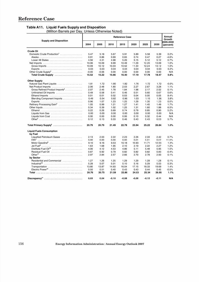
7/28/2019 2007 Annual Energy Outlook
http://slidepdf.com/reader/full/2007-annual-energy-outlook 165/243
156 Energy Information Administration / Annual Energy Outlook 2007
Reference Case
Table A11. Liquid Fuels Supply and Disposition(Million Barrels per Day, Unless Otherwise Noted)
Supply and Disposition
Reference Case AnnualGrowth
2005-2030(percent)2004 2005 2010 2015 2020 2025 2030
Crude Oil
Domestic Crude Production1 . . . . . . . . . . . . . . . . . 5.47 5.18 5.67 5.91 5.89 5.58 5.39 0.2%
Alaska . . . . . . . . . . . . . . . . . . . . . . . . . . . . . . . . . 0.91 0.86 0.69 0.65 0.74 0.47 0.27 -4.6%
Lower 48 States . . . . . . . . . . . . . . . . . . . . . . . . . 4.56 4.31 4.98 5.26 5.15 5.12 5.12 0.7%
Net Imports . . . . . . . . . . . . . . . . . . . . . . . . . . . . . . 10.06 10.09 9.99 10.49 11.29 12.20 13.09 1.0%
Gross Imports . . . . . . . . . . . . . . . . . . . . . . . . . . . 10.09 10.12 10.03 10.52 11.33 12.24 13.12 1.0%
Exports . . . . . . . . . . . . . . . . . . . . . . . . . . . . . . . . 0.03 0.03 0.04 0.04 0.04 0.04 0.03 0.2%
Other Crude Supply2 . . . . . . . . . . . . . . . . . . . . . . . -0.00 -0.06 0.00 0.00 0.00 0.00 0.00 N/A
Total Crude Supply . . . . . . . . . . . . . . . . . . . . . 15.52 15.22 15.66 16.40 17.19 17.78 18.47 0.8%
Other Supply
Natural Gas Plant Liquids . . . . . . . . . . . . . . . . . . . 1.81 1.72 1.80 1.82 1.76 1.72 1.72 -0.0%
Net Product Imports . . . . . . . . . . . . . . . . . . . . . . . 2.06 2.48 1.80 2.03 2.27 2.67 3.28 1.1%
Gross Refined Product Imports3 . . . . . . . . . . . . . 2.07 2.45 1.78 1.84 1.98 2.17 2.52 0.1%
Unfinished Oil Imports . . . . . . . . . . . . . . . . . . . . 0.49 0.58 0.41 0.46 0.51 0.60 0.67 0.6%
Ethanol Imports . . . . . . . . . . . . . . . . . . . . . . . . . 0.01 0.01 0.02 0.03 0.04 0.05 0.05 8.4%
Blending Component Imports . . . . . . . . . . . . . . . 0.49 0.54 0.82 0.96 1.03 1.15 1.36 3.8%Exports . . . . . . . . . . . . . . . . . . . . . . . . . . . . . . . . 0.96 1.07 1.23 1.25 1.29 1.30 1.33 0.9%
Refinery Processing Gain4 . . . . . . . . . . . . . . . . . . 1.05 0.99 1.21 1.27 1.41 1.45 1.49 1.7%
Other Inputs . . . . . . . . . . . . . . . . . . . . . . . . . . . . . . 0.34 0.39 1.02 1.25 1.31 1.60 1.88 6.5%
Ethanol . . . . . . . . . . . . . . . . . . . . . . . . . . . . . . . . 0.22 0.26 0.69 0.74 0.79 0.85 0.90 5.2%
Liquids from Gas . . . . . . . . . . . . . . . . . . . . . . . . 0.00 0.00 0.00 0.00 0.00 0.00 0.00 N/A
Liquids from Coal . . . . . . . . . . . . . . . . . . . . . . . . 0.00 0.00 0.00 0.06 0.10 0.32 0.44 N/A
Other5 . . . . . . . . . . . . . . . . . . . . . . . . . . . . . . . . . 0.12 0.13 0.33 0.46 0.43 0.43 0.53 5.7%
Total Primary Supply6 . . . . . . . . . . . . . . . . . . . . . . 20.79 20.79 21.49 22.78 23.94 25.22 26.84 1.0%
Liquid Fuels Consumption
by Fuel
Liquefied Petroleum Gases . . . . . . . . . . . . . . . . 2.13 2.03 2.22 2.23 2.26 2.33 2.42 0.7%
E857 . . . . . . . . . . . . . . . . . . . . . . . . . . . . . . . . . . 0.00 0.00 0.00 0.00 0.01 0.01 0.02 11.9%
Motor Gasoline8 . . . . . . . . . . . . . . . . . . . . . . . . . 9.10 9.16 9.53 10.18 10.93 11.71 12.53 1.3%
Jet Fuel9 . . . . . . . . . . . . . . . . . . . . . . . . . . . . . . . 1.63 1.68 1.95 2.10 2.19 2.22 2.27 1.2%
Distillate Fuel Oil10 . . . . . . . . . . . . . . . . . . . . . . . 4.06 4.12 4.53 4.86 5.11 5.48 5.95 1.5%Residual Fuel Oil . . . . . . . . . . . . . . . . . . . . . . . . 0.87 0.92 0.79 0.82 0.82 0.82 0.83 -0.4%
Other11 . . . . . . . . . . . . . . . . . . . . . . . . . . . . . . . . 2.97 2.84 2.57 2.66 2.70 2.78 2.93 0.1%
by Sector
Residential and Commercial . . . . . . . . . . . . . . . 1.27 1.26 1.25 1.29 1.29 1.28 1.28 0.1%
Industrial12 . . . . . . . . . . . . . . . . . . . . . . . . . . . . . 5.28 5.07 5.01 5.10 5.16 5.29 5.53 0.3%
Transportation . . . . . . . . . . . . . . . . . . . . . . . . . . 13.80 13.87 14.93 16.04 17.15 18.33 19.69 1.4%
Electric Power13 . . . . . . . . . . . . . . . . . . . . . . . . . 0.50 0.51 0.40 0.43 0.43 0.44 0.45 -0.5%
Total . . . . . . . . . . . . . . . . . . . . . . . . . . . . . . . . . . . 20.76 20.75 21.59 22.86 24.03 25.34 26.95 1.1%
Discrepancy14 . . . . . . . . . . . . . . . . . . . . . . . . . . . . . 0.03 0.04 -0.10 -0.08 -0.09 -0.12 -0.11 N/A

7/28/2019 2007 Annual Energy Outlook
http://slidepdf.com/reader/full/2007-annual-energy-outlook 166/243
Energy Information Administration / Annual Energy Outlook 2007 157
Reference Case
Table A11. Liquid Fuels Supply and Disposition (Continued)(Million Barrels per Day, Unless Otherwise Noted)
Supply and Disposition
Reference Case AnnualGrowth
2005-2030(percent)2004 2005 2010 2015 2020 2025 2030
Domestic Refinery Distillation Capacity15 . . . . . . . . . 16.9 17.1 17.8 18.0 18.7 19.4 20.0 0.6%
Capacity Utilization Rate (percent)16 . . . . . . . . . . . . 93.0 91.0 89.1 92.2 93.4 93.1 93.5 0.1%
Net Import Share of Product Supplied (percent) . . . 58.3 60.5 54.9 55.0 56.6 59.0 61.0 0.0%
Net Expenditures for Imported Crude Oil and
Petroleum Products (billion 2005 dollars) . . . . . . . 179.47 236.65 222.76 203.97 229.80 264.31 300.51 1.0%
1Includes lease condensate.2Strategic petroleum reserve stock additions plus unaccounted for crude oil and crude stock withdrawals minus crude product supplied.3Includes other hydrocarbons and alcohols.4Represents volumetric gain in refinery distillation and cracking processes.5Includes petroleum product stock withdrawals, domestic sources of blending components, other hydrocarbons, ethers, and renewable fuels such as biodiesel.6Total crude supply plus natural gas plant liquids, other inputs, refinery processing gain, and net product imports.7E85 refers to a blend of 85 percent ethanol (renewable) and 15 percent motor gasoline (nonrenewable). To address cold starting issues, the percentage of
ethanol actually varies seasonally. The annual average ethanol content of 74 percent is used for this forecast.8Includes ethanol and ethers blended into gasoline.9Includes only kerosene type.10Includes distillate fuel oil and kerosene from petroleum and biomass feedstocks.11
Includes aviation gasoline, petrochemical feedstocks, lubricants, waxes, asphalt, road oil, still gas, special naphthas, petroleum coke, crude oil productsupplied, tire-derived fuel, methanol, liquid hydrogen,and miscellaneous petroleum products.12Includes consumption for combined heat and power, which produces electricity and other useful thermal energy.13Includes consumption of energy by electricity-only and combined heat and power plants whose primary business is to sell electricity, or electricity and heat, to
the public. Includes small power producers and exempt wholesale generators.14Balancing item. Includes unaccounted for supply, losses, and gains.15End-of-year operable capacity.16Rate is calculated by dividing the gross annual input to atmospheric crude oil distillation units by their operable refining capacity in barrels per calendar day.N/A = Not applicable.Note: Totals may not equal sum of components due to independent rounding. Data for 2004 and 2005 are model results and may differ slightly from official EIA
data reports.Sources: 2004 and 2005 imported crude oil price and petroleum product supplied based on: Energy Information Administration (EIA), Annual Energy Review
2005 , DOE/EIA-0384(2005) (Washington, DC, July 2006). 2004 and 2005 imported low sulfur light crude oil price: EIA, Form EIA-856, “Monthly Foreign Crude OilAcquisition Report.” Other 2004 data: EIA, Petroleum Supply Annual 2004, DOE/EIA-0340(2004)/1 (Washington, DC, June 2005). Other 2005 data: EIA,Petroleum Supply Annual 2005, DOE/EIA-0340(2005)/1 (Washington, DC, October 2006). Projections: EIA, AEO2007 National Energy Modeling System runAEO2007.D112106A.

7/28/2019 2007 Annual Energy Outlook
http://slidepdf.com/reader/full/2007-annual-energy-outlook 167/243
158 Energy Information Administration / Annual Energy Outlook 2007
Reference Case
Table A12. Petroleum Product Prices(2005 Cents per Gallon, Unless Otherwise Noted)
Sector and Fuel
Reference Case AnnualGrowth
2005-2030(percent)2004 2005 2010 2015 2020 2025 2030
Crude Oil Prices (2005 dollars per barrel)
Imported Low Sulfur Light Crude Oil1 . . . . . . . . 42.87 56.76 57.47 49.87 52.04 56.37 59.12 0.2%
Imported Crude Oil1 . . . . . . . . . . . . . . . . . . . . . . 37.09 49.19 51.20 44.61 46.47 49.57 51.63 0.2%
Delivered Sector Product Prices
Residential
Liquefied Petroleum Gases . . . . . . . . . . . . . . 156.9 166.3 204.0 197.2 199.8 202.8 206.1 0.9%
Distillate Fuel Oil . . . . . . . . . . . . . . . . . . . . . . 178.8 204.3 206.3 174.7 182.3 188.1 195.9 -0.2%
Commercial
Distillate Fuel Oil . . . . . . . . . . . . . . . . . . . . . . 145.0 175.4 175.5 147.9 156.5 163.4 171.7 -0.1%
Residual Fuel Oil . . . . . . . . . . . . . . . . . . . . . . 93.5 126.0 112.8 97.2 105.8 107.3 109.4 -0.6%
Residual Fuel Oil (2005 dollars per barrel) . . 39.29 52.90 47.39 40.83 44.44 45.08 45.97 -0.6%
Industrial2
Liquefied Petroleum Gases . . . . . . . . . . . . . . 96.3 146.2 141.5 134.1 137.1 139.8 142.6 -0.1%Distillate Fuel Oil . . . . . . . . . . . . . . . . . . . . . . 152.2 181.1 178.1 156.5 165.3 173.2 181.8 0.0%
Residual Fuel Oil . . . . . . . . . . . . . . . . . . . . . . 86.4 116.3 142.2 122.9 133.4 138.6 143.5 0.8%
Residual Fuel Oil (2005 dollars per barrel) . . 36.30 48.86 59.74 51.64 56.04 58.21 60.25 0.8%
Transportation
Liquefied Petroleum Gases . . . . . . . . . . . . . . 169.5 206.1 209.8 202.4 203.9 206.4 209.3 0.1%
Ethanol (E85)3 . . . . . . . . . . . . . . . . . . . . . . . . 196.5 217.1 198.5 187.3 192.1 198.2 200.4 -0.3%
Ethanol Wholesale Price . . . . . . . . . . . . . . . . 177.2 180.4 181.4 166.0 168.2 171.1 170.2 -0.2%
Motor Gasoline4 . . . . . . . . . . . . . . . . . . . . . . . 195.2 231.6 217.3 194.9 201.9 210.2 215.4 -0.3%
Jet Fuel5 . . . . . . . . . . . . . . . . . . . . . . . . . . . . . 124.4 177.4 147.2 133.5 141.8 149.8 158.6 -0.4%
Diesel Fuel (distillate fuel oil)6 . . . . . . . . . . . . 187.1 241.3 230.4 203.6 211.2 218.1 225.7 -0.3%
Residual Fuel Oil . . . . . . . . . . . . . . . . . . . . . . 72.7 82.4 120.5 105.4 110.2 118.2 123.8 1.6%
Residual Fuel Oil (2005 dollars per barrel) . . 30.51 34.62 50.60 44.27 46.27 49.65 52.02 1.6%
Electric Power7
Distillate Fuel Oil . . . . . . . . . . . . . . . . . . . . . . 132.0 157.9 162.3 128.4 136.5 142.2 149.6 -0.2%
Residual Fuel Oil . . . . . . . . . . . . . . . . . . . . . . 74.7 104.2 98.5 83.8 91.0 98.5 102.5 -0.1%Residual Fuel Oil (2005 dollars per barrel) . . 31.38 43.76 41.37 35.20 38.24 41.37 43.05 -0.1%
Refined Petroleum Product Prices8
Liquefied Petroleum Gases . . . . . . . . . . . . . . 109.3 150.7 155.3 148.6 151.9 154.8 157.7 0.2%
Motor Gasoline4 . . . . . . . . . . . . . . . . . . . . . . . 195.0 231.1 217.3 194.9 201.8 210.2 215.4 -0.3%
Jet Fuel5 . . . . . . . . . . . . . . . . . . . . . . . . . . . . . 124.4 177.4 147.2 133.5 141.8 149.8 158.6 -0.4%
Distillate Fuel Oil . . . . . . . . . . . . . . . . . . . . . . 178.3 223.9 215.9 191.0 199.4 207.0 215.5 -0.2%
Residual Fuel Oil . . . . . . . . . . . . . . . . . . . . . . 76.3 98.6 113.9 98.0 104.7 111.9 116.6 0.7%
Residual Fuel Oil (2005 dollars per barrel) . . 32.05 41.42 47.84 41.16 43.98 46.99 48.96 0.7%
Average . . . . . . . . . . . . . . . . . . . . . . . . . . . 168.6 204.5 195.0 175.7 183.4 191.3 198.1 -0.1%
1Weighted average price delivered to U.S. refiners.2Includes energy for combined heat and power plants, except those whose primary business is to sell electricity, or electricity and heat, to the public.3E85 refers to a blend of 85 percent ethanol (renewable) and 15 percent motor gasoline (nonrenewable). To address cold starting issues, the percentage of
ethanol actually varies seasonally. The annual average ethanol content of 74 percent is used for this forecast.4Sales weighted-average price for all grades. Includes Federal, State and local taxes.5Includes only kerosene type.6Diesel fuel for on-road use. Includes Federal and State taxes while excluding county and local taxes.7Includes electricity-only and combined heat and power plants whose primary business is to sell electricity, or electricity and heat, to the public. Includes small
power producers and exempt wholesale generators.8Weighted averages of end-use fuel prices are derived from the prices in each sector and the corresponding sectoral consumption.Note: Data for 2004 and 2005 are model results and may differ slightly from official EIA data reports.Sources: 2004 and 2005 imported low sulfur light crude oil price: Energy Information Administration (EIA), Form EIA-856, “Monthly Foreign Crude Oil
Acquisition Report.” 2004 and 2005 imported crude oil price: EIA, Annual Energy Review 2005 , DOE/EIA-0384(2005) (Washington, DC, July 2006). 2004 and2005 prices for motor gasoline, distillate fuel oil, and jet fuel are based on: EIA, Petroleum Marketing Annual 2005 , DOE/EIA-0487(2005) (Washington, DC, August2006). 2004 and 2005 residential, commercial, industrial, and transportation sector petroleum product prices are derived from: EIA, Form EIA-782A,“Refiners’/Gas Plant Operators’ Monthly Petroleum Product Sales Report.” 2004 and 2005 electric power prices based on: Federal Energy RegulatoryCommission, FERC Form 423, “Monthly Report of Cost and Quality of Fuels for Electric Plants.” 2004 and 2005 ethanol prices derived from weekly spot prices inthe Oxy Fuel News. 2004 and 2005 wholesale ethanol prices derived from Bloomburg U.S. average rack price. Projections: EIA, AEO2007 National EnergyModeling System run AEO2007.D112106A.

7/28/2019 2007 Annual Energy Outlook
http://slidepdf.com/reader/full/2007-annual-energy-outlook 168/243
Energy Information Administration / Annual Energy Outlook 2007 159
Reference Case
Table A13. Natural Gas Supply, Disposition, and Prices(Trillion Cubic Feet per Year, Unless Otherwise Noted)
Supply, Disposition, and Prices
Reference Case AnnualGrowth
2005-2030(percent)2004 2005 2010 2015 2020 2025 2030
Production
Dry Gas Production1 . . . . . . . . . . . . . . . . . . . . . 18.76 18.23 19.35 19.60 20.79 20.59 20.53 0.5%
Supplemental Natural Gas2 . . . . . . . . . . . . . . . . 0.07 0.07 0.07 0.07 0.07 0.07 0.07 0.1%
Net Imports . . . . . . . . . . . . . . . . . . . . . . . . . . . . . 3.40 3.57 4.55 5.62 5.35 5.58 5.45 1.7%
Pipeline3 . . . . . . . . . . . . . . . . . . . . . . . . . . . . . . 2.81 3.01 2.74 2.63 1.65 1.20 0.92 -4.6%
Liquefied Natural Gas . . . . . . . . . . . . . . . . . . . . 0.59 0.57 1.81 2.99 3.69 4.38 4.53 8.7%
Total Supply . . . . . . . . . . . . . . . . . . . . . . . . . . . . 22.22 21.87 23.97 25.29 26.21 26.24 26.06 0.7%
Consumption by Sector
Residential . . . . . . . . . . . . . . . . . . . . . . . . . . . . . 4.87 4.84 5.03 5.19 5.27 5.29 5.31 0.4%
Commercial . . . . . . . . . . . . . . . . . . . . . . . . . . . . 3.13 3.05 3.22 3.53 3.75 3.98 4.24 1.3%
Industrial4 . . . . . . . . . . . . . . . . . . . . . . . . . . . . . . 7.22 6.64 7.63 7.67 8.02 8.42 8.65 1.1%
Natural-Gas-to-Liquids Heat and Power5 . . . . . 0.00 0.00 0.00 0.00 0.00 0.00 0.00 N/A
Natural Gas to Liquids Production6 . . . . . . . . . . 0.00 0.00 0.00 0.00 0.00 0.00 0.00 N/A
Electric Power7 . . . . . . . . . . . . . . . . . . . . . . . . . 5.48 5.78 6.38 7.11 7.19 6.59 5.92 0.1%
Transportation8 . . . . . . . . . . . . . . . . . . . . . . . . . 0.03 0.03 0.06 0.08 0.09 0.11 0.12 5.7%
Pipeline Fuel . . . . . . . . . . . . . . . . . . . . . . . . . . . 0.57 0.56 0.64 0.68 0.76 0.77 0.77 1.3%
Lease and Plant Fuel9 . . . . . . . . . . . . . . . . . . . . 1.10 1.07 1.07 1.07 1.17 1.14 1.12 0.2%
Total . . . . . . . . . . . . . . . . . . . . . . . . . . . . . . . . 22.39 21.98 24.02 25.32 26.26 26.30 26.12 0.7%
Discrepancy10 . . . . . . . . . . . . . . . . . . . . . . . . . . . -0.17 -0.11 -0.05 -0.03 -0.05 -0.06 -0.06 N/A
Natural Gas Prices
(2005 dollars per million Btu)
Henry Hub Spot Price . . . . . . . . . . . . . . . . . . . 6.08 8.60 6.28 5.46 5.71 6.14 6.52 -1.1%
Average Lower 48 Wellhead Price11 . . . . . . . 5.63 7.29 5.59 4.84 5.07 5.46 5.80 -0.9%
(2005 dollars per thousand cubic feet)
Average Lower 48 Wellhead Price11 . . . . . . . 5.80 7.51 5.76 4.99 5.22 5.62 5.98 -0.9%
Delivered Prices
Residential . . . . . . . . . . . . . . . . . . . . . . . . . . . 11.05 12.80 11.31 10.55 10.86 11.30 11.77 -0.3%Commercial . . . . . . . . . . . . . . . . . . . . . . . . . . 9.69 11.54 9.62 8.73 8.93 9.23 9.58 -0.7%
Industrial4 . . . . . . . . . . . . . . . . . . . . . . . . . . . . 6.67 8.41 6.62 5.82 6.08 6.40 6.76 -0.9%
Electric Power7 . . . . . . . . . . . . . . . . . . . . . . . . 6.27 8.42 6.40 5.66 5.93 6.22 6.51 -1.0%
Transportation12 . . . . . . . . . . . . . . . . . . . . . . . 12.28 15.20 14.38 13.25 13.36 13.62 13.86 -0.4%
Average13 . . . . . . . . . . . . . . . . . . . . . . . . . . 8.06 9.94 8.07 7.28 7.54 7.91 8.33 -0.7%
1Marketed production (wet) minus extraction losses.2Synthetic natural gas, propane air, coke oven gas, refinery gas, biomass gas, air injected for Btu stabilization, and manufactured gas commingled and
distributed with natural gas.3Includes any natural gas regasified in the Bahamas and transported via pipeline to Florida.4Includes energy for combined heat and power plants, except those whose primary business is to sell electricity, or electricity and heat, to the public.5Includes any natural gas used in the process of converting natural gas to liquid fuel that is not actually converted.6Includes any natural gas that is converted into liquid fuel.7Includes consumption of energy by electricity-only and combined heat and power plants whose primary business is to sell electricity, or electricity and heat, to
the public. Includes small power producers and exempt wholesale generators.8Compressed natural gas used as vehicle fuel.9Represents natural gas used in well, field, and lease operations, and in natural gas processing plant machinery.10Balancing item. Natural gas lost as a result of converting flow data measured at varying temperatures and pressures to a standard temperature and pressure
and the merger of different data reporting systems which vary in scope, format, definition, and respondent type. In addition, 2004 and 2005 values include net
storage injections.11Represents lower 48 onshore and offshore supplies.12Compressed natural gas used as a vehicle fuel. Price includes estimated motor vehicle fuel taxes and estimated dispensing costs or charges.13Weighted average prices. Weights used are the sectoral consumption values excluding lease, plant, and pipeline fuel.N/A = Not applicable.Note: Totals may not equal sum of components due to independent rounding. Data for 2004 and 2005 are model results and may differ slightly from official EIA
data reports.Sources: 2004 supply values; and lease, plant, and pipeline fuel consumption: Energy Information Administration (EIA), Natural Gas Annual 2004 , DOE/EIA-
0131(2004) (Washington, DC, December 2005). 2005 supply values; and lease, plant, and pipeline fuel consumption; and wellhead price: EIA, Natural Gas Monthly , DOE/EIA-0130(2006/04) (Washington, DC, April 2006). Other 2004 and 2005 consumption based on: EIA, Annual Energy Review 2005 , DOE/EIA-0384(2005) (Washington, DC, July 2006). 2004 wellhead price: Minerals Management Service and EIA, Natural Gas Annual 2004 , DOE/EIA-0131(2004)(Washington, DC, December 2005). 2004 residential and commercial delivered prices: EIA, Natural Gas Annual 2004 , DOE/EIA-0131(2004) (Washington, DC,December 2005). 2005 residential and commercial delivered prices: EIA, Natural Gas Monthly , DOE/EIA-0130(2006/04) (Washington, DC, April 2006). 2004 and2005 electric power prices: EIA, Electric Power Monthly , DOE/EIA-0226, May 2005 through April 2006, Table 4.11.A. 2004 and 2005 industrial delivered pricesare estimated based on: EIA, Manufacturing Energy Consumption Survey 1994 and industrial and wellhead prices from the Natural Gas Annual 2004 , DOE/EIA-0131(2004) (Washington, DC, December 2005) and the Natural Gas Monthly , DOE/EIA-0130(2006/04) (Washington, DC, April 2006). 2004 transportation sectordelivered prices are based on: EIA, Natural Gas Annual 2004 , DOE/EIA-0131(2004) (Washington, DC, December 2005) and estimated state taxes, federal taxes,and dispensing costs or charges. 2005 transportation sector delivered prices are model results. Projections: EIA, AEO2007 National Energy Modeling Systemrun AEO2007.D112106A.

7/28/2019 2007 Annual Energy Outlook
http://slidepdf.com/reader/full/2007-annual-energy-outlook 169/243
160 Energy Information Administration / Annual Energy Outlook 2007
Reference Case
Table A14. Oil and Gas Supply
Production and Supply
Reference Case AnnualGrowth
2005-2030(percent)2004 2005 2010 2015 2020 2025 2030
Crude Oil
Lower 48 Average Wellhead Price1
(2005 dollars per barrel) . . . . . . . . . . . . . . . . . . . 38.69 50.76 48.54 41.71 44.88 48.37 51.25 0.0%
Production (million barrels per day)2
United States Total . . . . . . . . . . . . . . . . . . . . . . . 5.45 5.18 5.67 5.91 5.89 5.58 5.39 0.2%
Lower 48 Onshore . . . . . . . . . . . . . . . . . . . . . . 2.94 2.89 2.93 2.91 2.94 2.95 2.92 0.0%
Lower 48 Offshore . . . . . . . . . . . . . . . . . . . . . . 1.61 1.42 2.05 2.35 2.21 2.16 2.20 1.8%
Alaska . . . . . . . . . . . . . . . . . . . . . . . . . . . . . . . . 0.91 0.86 0.69 0.65 0.74 0.47 0.27 -4.6%
Lower 48 End of Year Reserves2
(billion barrels) . . . . . . . . . . . . . . . . . . . . . . . . . . . 18.27 16.98 19.53 20.46 19.98 19.47 17.94 0.2%
Natural Gas
Lower 48 Average Wellhead Price1
(2005 dollars per million Btu)
Henry Hub Spot Price . . . . . . . . . . . . . . . . . . . . . 6.08 8.60 6.28 5.46 5.71 6.14 6.52 -1.1%Average Lower 48 Wellhead Price1 . . . . . . . . . . 5.63 7.29 5.59 4.84 5.07 5.46 5.80 -0.9%
(2005 dollars per thousand cubic feet)
Average Lower 48 Wellhead Price1 . . . . . . . . . . 5.80 7.51 5.76 4.99 5.22 5.62 5.98 -0.9%
Dry Production (trillion cubic feet)3
United States Total . . . . . . . . . . . . . . . . . . . . . . . 18.76 18.23 19.35 19.60 20.79 20.59 20.53 0.5%
Lower 48 Onshore . . . . . . . . . . . . . . . . . . . . . . 14.10 14.36 15.22 14.79 14.66 14.84 15.13 0.2%
Associated-Dissolved4 . . . . . . . . . . . . . . . . . . 1.40 1.43 1.39 1.32 1.28 1.23 1.19 -0.8%
Non-Associated . . . . . . . . . . . . . . . . . . . . . . . 12.69 12.93 13.83 13.46 13.38 13.61 13.94 0.3%
Conventional . . . . . . . . . . . . . . . . . . . . . . . 5.19 4.94 5.27 4.71 4.30 3.98 3.75 -1.1%
Unconventional . . . . . . . . . . . . . . . . . . . . . . 7.50 7.99 8.56 8.75 9.09 9.63 10.19 1.0%
Lower 48 Offshore . . . . . . . . . . . . . . . . . . . . . . 4.23 3.41 3.88 4.56 4.09 3.55 3.25 -0.2%
Associated-Dissolved4 . . . . . . . . . . . . . . . . . . 0.88 0.71 0.92 1.13 1.05 0.94 0.85 0.7%
Non-Associated . . . . . . . . . . . . . . . . . . . . . . . 3.35 2.69 2.96 3.43 3.04 2.61 2.40 -0.5%
Alaska . . . . . . . . . . . . . . . . . . . . . . . . . . . . . . . . 0.44 0.45 0.25 0.25 2.05 2.20 2.16 6.4%
Lower 48 End of Year Dry Reserves3
(trillion cubic feet) . . . . . . . . . . . . . . . . . . . . . . . . 184.11 189.91 205.23 210.31 208.32 208.61 210.60 0.4%
Supplemental Gas Supplies (trillion cubic feet)5 0.07 0.07 0.07 0.07 0.07 0.07 0.07 0.1%
Total Lower 48 Wells Drilled (thousands) . . . . . . 32.67 41.66 37.17 32.01 31.84 32.78 30.65 -1.2%
1Represents lower 48 onshore and offshore supplies.2Includes lease condensate.3Marketed production (wet) minus extraction losses.4Gas which occurs in crude oil reservoirs either as free gas (associated) or as gas in solution with crude oil (dissolved).5Synthetic natural gas, propane air, coke oven gas, refinery gas, biomass gas, air injected for Btu stabilization, and manufactured gas commingled and
distributed with natural gas.Note: Totals may not equal sum of components due to independent rounding. Data for 2004 and 2005 are model results and may differ slightly from official EIA
data reports.Sources: 2004 and 2005 crude oil lower 48 average wellhead price: Energy Information Administration (EIA), Petroleum Marketing Annual 2005 , DOE/EIA-
0487(2005) (Washington, DC, August 2006). 2004 and 2005 lower 48 onshore, lower 48 offshore, and Alaska crude oil production: EIA, Petroleum Supply Annual
2005, DOE/EIA-0340(2005)/1 (Washington, DC, October 2006). 2004 U.S. crude oil and natural gas reserves: EIA, U.S. Crude Oil, Natural Gas, and Natural Gas Liquids Reserves , DOE/EIA-0216(2004) (Washington, DC, November 2005). 2004 Alaska and total natural gas production, and supplemental gas supplies: EIA,Natural Gas Annual 2004 , DOE/EIA-0131(2004) (Washington, DC, December 2005). 2004 natural gas lower 48 average wellhead price: Minerals ManagementService and EIA, Natural Gas Annual 2004 , DOE/EIA-0131(2004) (Washington, DC, December 2005). 2005 natural gas lower 48 average wellhead price, Alaskaand total natural gas production, and supplemental gas supplies: EIA, Natural Gas Monthly , DOE/EIA-0130(2006/04) (Washington, DC, April 2006). Other 2004and 2005 values: EIA, Office of Integrated Analysis and Forecasting. Projections: EIA, AEO2007 National Energy Modeling System run AEO2007.D112106A.

7/28/2019 2007 Annual Energy Outlook
http://slidepdf.com/reader/full/2007-annual-energy-outlook 170/243
Energy Information Administration / Annual Energy Outlook 2007 161
Reference Case
Table A15. Coal Supply, Disposition, and Prices(Million Short Tons per Year, Unless Otherwise Noted)
Supply, Disposition, and Prices
Reference Case AnnualGrowth
2005-2030(percent)2004 2005 2010 2015 2020 2025 2030
Production1
Appalachia . . . . . . . . . . . . . . . . . . . . . . . . . . . . . 391 397 381 371 348 351 373 -0.3%
Interior . . . . . . . . . . . . . . . . . . . . . . . . . . . . . . . . 146 149 171 199 203 215 247 2.0%
West . . . . . . . . . . . . . . . . . . . . . . . . . . . . . . . . . 575 585 637 697 772 951 1072 2.5%
East of the Mississippi . . . . . . . . . . . . . . . . . . . . 485 494 498 507 487 499 545 0.4%
West of the Mississippi . . . . . . . . . . . . . . . . . . . 627 638 691 759 837 1018 1146 2.4%
Total . . . . . . . . . . . . . . . . . . . . . . . . . . . . . . . . 1112 1131 1189 1266 1323 1517 1691 1.6%
Waste Coal Supplied2 . . . . . . . . . . . . . . . . . . . . . 11 13 13 13 13 13 13 -0.0%
Net Imports
Imports3 . . . . . . . . . . . . . . . . . . . . . . . . . . . . . . . 26 29 37 42 72 79 95 4.9%
Exports . . . . . . . . . . . . . . . . . . . . . . . . . . . . . . . 48 50 44 37 31 27 27 -2.4%
Total . . . . . . . . . . . . . . . . . . . . . . . . . . . . . . . . -22 -21 -7 5 41 52 68 N/A
Total Supply4
. . . . . . . . . . . . . . . . . . . . . . . . . . . . 1101 1124 1195 1284 1377 1582 1772 1.8%
Consumption by Sector
Residential and Commercial . . . . . . . . . . . . . . . 5 5 5 5 5 5 5 -0.3%
Coke Plants . . . . . . . . . . . . . . . . . . . . . . . . . . . . 24 23 22 21 21 21 21 -0.5%
Other Industrial5 . . . . . . . . . . . . . . . . . . . . . . . . . 62 61 64 62 63 63 64 0.2%
Coal-to-Liquids Heat and Power . . . . . . . . . . . . 0 0 0 8 13 42 57 N/A
Coal to Liquids Production . . . . . . . . . . . . . . . . 0 0 0 8 13 40 55 N/A
Electric Power6 . . . . . . . . . . . . . . . . . . . . . . . . . 1016 1039 1104 1178 1262 1411 1570 1.7%
Total . . . . . . . . . . . . . . . . . . . . . . . . . . . . . . . . 1107 1128 1195 1282 1377 1582 1772 1.8%
Discrepancy and Stock Change7 . . . . . . . . . . . -6 -5 0 1 0 0 0 N/A
Average Minemouth Price8
(2005 dollars per short ton) . . . . . . . . . . . . . . . . 20.68 23.34 24.20 22.41 21.58 21.55 22.60 -0.1%
(2005 dollars per million Btu) . . . . . . . . . . . . . . 1.01 1.15 1.18 1.11 1.08 1.09 1.15 -0.0%
Delivered Prices (2005 dollars per short ton)9
Coke Plants . . . . . . . . . . . . . . . . . . . . . . . . . . . . 63.36 83.79 84.86 74.51 74.25 73.93 75.55 -0.4%
Other Industrial5 . . . . . . . . . . . . . . . . . . . . . . . . . 40.49 47.63 48.86 47.45 46.55 47.60 48.54 0.1%
Coal to Liquids . . . . . . . . . . . . . . . . . . . . . . . . . . N/A N/A N/A 13.79 15.05 19.82 21.89 N/A
Electric Power
(2005 dollars per short ton) . . . . . . . . . . . . . . 28.12 30.83 34.17 31.84 31.39 32.20 33.52 0.3%
(2005 dollars per million Btu) . . . . . . . . . . . . . 1.40 1.53 1.71 1.60 1.58 1.63 1.69 0.4%
Average . . . . . . . . . . . . . . . . . . . . . . . . . . 29.58 32.82 35.89 33.10 32.42 32.72 33.82 0.1%
Exports10 . . . . . . . . . . . . . . . . . . . . . . . . . . . . . . 55.75 67.10 69.35 64.51 64.49 61.66 63.81 -0.2%
1Includes anthracite, bituminous coal, and lignite.2Includes waste coal consumed by the electric power and industrial sectors. Waste coal supplied is counted as a supply-side item to balance the same amount
of waste coal included in the consumption data.3Excludes imports to Puerto Rico and the U.S. Virgin Islands.4Production plus waste coal supplied plus net imports.5Includes consumption for combined heat and power plants, except those plants whose primary business is to sell electricity, or electricity and heat, to the
public. Excludes all coal use in the coal-to-liquids process.6Includes all electricity-only and combined heat and power plants whose primary business is to sell electricity, or electricity and heat, to the public.7
Balancing item: the sum of production, net imports, and waste coal supplied minus total consumption.8Includes reported prices for both open market and captive mines.9Prices weighted by consumption; weighted average excludes residential and commercial prices, and export free-alongside-ship (f.a.s.) prices.10F.a.s. price at U.S. port of exit.N/A = Not applicable.Btu = British thermal unit.Note: Totals may not equal sum of components due to independent rounding. Data for 2004 and 2005 are model results and may differ slightly from official EIA
data reports.Sources: 2004 and 2005 data based on: Energy Information Administration (EIA), Annual Coal Report 2005 , DOE/EIA-0584(2005) (Washington, DC, October
2006); EIA, Quarterly Coal Report, October-December 2005 , DOE/EIA-0121(2005/4Q) (Washington, DC, March 2006); and EIA, AEO2007 National EnergyModeling System run AEO2007.D112106A. Projections: EIA, AEO2007 National Energy Modeling System run AEO2007.D112106A.
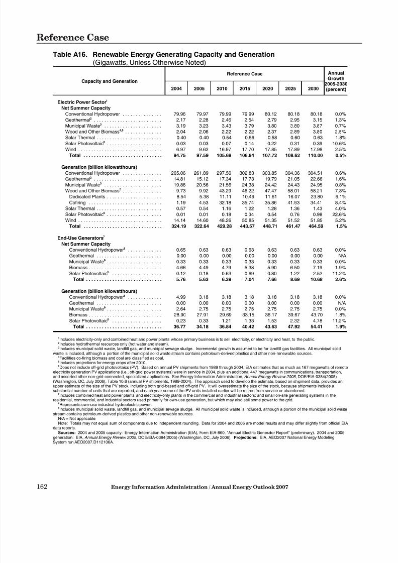
7/28/2019 2007 Annual Energy Outlook
http://slidepdf.com/reader/full/2007-annual-energy-outlook 171/243
162 Energy Information Administration / Annual Energy Outlook 2007
Reference Case
Table A16. Renewable Energy Generating Capacity and Generation(Gigawatts, Unless Otherwise Noted)
Capacity and Generation
Reference Case AnnualGrowth
2005-2030(percent)2004 2005 2010 2015 2020 2025 2030
Electric Power Sector1
Net Summer Capacity
Conventional Hydropower . . . . . . . . . . . . . . . 79.96 79.97 79.99 79.99 80.12 80.18 80.18 0.0%
Geothermal2 . . . . . . . . . . . . . . . . . . . . . . . . . . 2.17 2.28 2.46 2.54 2.79 2.95 3.15 1.3%
Municipal Waste3 . . . . . . . . . . . . . . . . . . . . . . 3.19 3.23 3.43 3.79 3.80 3.80 3.87 0.7%
Wood and Other Biomass4,5 . . . . . . . . . . . . . . 2.04 2.06 2.22 2.22 2.37 2.89 3.80 2.5%
Solar Thermal . . . . . . . . . . . . . . . . . . . . . . . . . 0.40 0.40 0.54 0.56 0.58 0.60 0.63 1.8%
Solar Photovoltaic6 . . . . . . . . . . . . . . . . . . . . . 0.03 0.03 0.07 0.14 0.22 0.31 0.39 10.6%
Wind . . . . . . . . . . . . . . . . . . . . . . . . . . . . . . . . 6.97 9.62 16.97 17.70 17.85 17.89 17.98 2.5%
Total . . . . . . . . . . . . . . . . . . . . . . . . . . . . . . 94.75 97.59 105.69 106.94 107.72 108.62 110.00 0.5%
Generation (billion kilowatthours)
Conventional Hydropower . . . . . . . . . . . . . . . 265.06 261.89 297.50 302.83 303.85 304.36 304.51 0.6%
Geothermal2 . . . . . . . . . . . . . . . . . . . . . . . . . . 14.81 15.12 17.34 17.73 19.79 21.05 22.66 1.6%
Municipal Waste3 . . . . . . . . . . . . . . . . . . . . . . 19.86 20.56 21.56 24.38 24.42 24.43 24.95 0.8%
Wood and Other Biomass5 . . . . . . . . . . . . . . . 9.73 9.92 43.29 46.22 47.47 58.01 58.21 7.3%
Dedicated Plants . . . . . . . . . . . . . . . . . . . . . 8.54 5.38 11.11 10.49 11.61 16.07 23.80 6.1%Cofiring . . . . . . . . . . . . . . . . . . . . . . . . . . . . 1.19 4.53 32.18 35.74 35.86 41.93 34.41 8.4%
Solar Thermal . . . . . . . . . . . . . . . . . . . . . . . . . 0.57 0.54 1.16 1.22 1.28 1.36 1.43 4.0%
Solar Photovoltaic6 . . . . . . . . . . . . . . . . . . . . . 0.01 0.01 0.18 0.34 0.54 0.76 0.98 22.6%
Wind . . . . . . . . . . . . . . . . . . . . . . . . . . . . . . . . 14.14 14.60 48.26 50.85 51.35 51.52 51.85 5.2%
Total . . . . . . . . . . . . . . . . . . . . . . . . . . . . . . 324.19 322.64 429.28 443.57 448.71 461.47 464.59 1.5%
End-Use Generators7
Net Summer Capacity
Conventional Hydropower8 . . . . . . . . . . . . . 0.65 0.63 0.63 0.63 0.63 0.63 0.63 0.0%
Geothermal . . . . . . . . . . . . . . . . . . . . . . . . . 0.00 0.00 0.00 0.00 0.00 0.00 0.00 N/A
Municipal Waste9 . . . . . . . . . . . . . . . . . . . . . 0.33 0.33 0.33 0.33 0.33 0.33 0.33 0.0%
Biomass . . . . . . . . . . . . . . . . . . . . . . . . . . . . 4.66 4.49 4.79 5.38 5.90 6.50 7.19 1.9%
Solar Photovoltaic6 . . . . . . . . . . . . . . . . . . . 0.12 0.18 0.63 0.69 0.80 1.22 2.52 11.2%
Total . . . . . . . . . . . . . . . . . . . . . . . . . . . . . 5.76 5.63 6.39 7.04 7.66 8.69 10.68 2.6%
Generation (billion kilowatthours)
Conventional Hydropower8 . . . . . . . . . . . . . 4.99 3.18 3.18 3.18 3.18 3.18 3.18 0.0%Geothermal . . . . . . . . . . . . . . . . . . . . . . . . . 0.00 0.00 0.00 0.00 0.00 0.00 0.00 N/A
Municipal Waste9 . . . . . . . . . . . . . . . . . . . . . 2.64 2.75 2.75 2.75 2.75 2.75 2.75 0.0%
Biomass . . . . . . . . . . . . . . . . . . . . . . . . . . . . 28.90 27.91 29.69 33.15 36.17 39.67 43.70 1.8%
Solar Photovoltaic6 . . . . . . . . . . . . . . . . . . . 0.23 0.33 1.21 1.33 1.53 2.32 4.78 11.2%
Total . . . . . . . . . . . . . . . . . . . . . . . . . . . . . 36.77 34.18 36.84 40.42 43.63 47.92 54.41 1.9%
1Includes electricity-only and combined heat and power plants whose primary business is to sell electricity, or electricity and heat, to the public.2Includes hydrothermal resources only (hot water and steam).3Includes municipal solid waste, landfill gas, and municipal sewage sludge. Incremental growth is assumed to be for landfill gas facilities. All municipal solid
waste is included, although a portion of the municipal solid waste stream contains petroleum-derived plastics and other non-renewable sources.4Facilities co-firing biomass and coal are classified as coal.5Includes projections for energy crops after 2010.6Does not include off-grid photovoltaics (PV). Based on annual PV shipments from 1989 through 2004, EIA estimates that as much as 167 megawatts of remote
electricity generation PV applications (i.e., off-grid power systems) were in service in 2004, plus an additional 447 megawatts in communications, transportation,and assorted other non-grid-connected, specialized applications. See Energy Information Administration, Annual Energy Review 2005 , DOE/EIA-0384(2005)(Washington, DC, July 2006), Table 10.6 (annual PV shipments, 1989-2004). The approach used to develop the estimate, based on shipment data, provides anupper estimate of the size of the PV stock, including both grid-based and off-grid PV. It will overestimate the size of the stock, because shipments include asubstantial number of units that are exported, and each year some of the PV units installed earlier will be retired from service or abandoned.
7Includes combined heat and power plants and electricity-only plants in the commercial and industrial sectors; and small on-site generating systems in theresidential, commercial, and industrial sectors used primarily for own-use generation, but which may also sell some power to the grid.
8Represents own-use industrial hydroelectric power.9Includes municipal solid waste, landfill gas, and municipal sewage sludge. All municipal solid waste is included, although a portion of the municipal solid waste
stream contains petroleum-derived plastics and other non-renewable sources.N/A = Not applicable.Note: Totals may not equal sum of components due to independent rounding. Data for 2004 and 2005 are model results and may differ slightly from official EIA
data reports.Sources: 2004 and 2005 capacity: Energy Information Administration (EIA), Form EIA-860, "Annual Electric Generator Report" (preliminary). 2004 and 2005
generation: EIA, Annual Energy Review 2005 , DOE/EIA-0384(2005) (Washington, DC, July 2006). Projections: EIA, AEO2007 National Energy ModelingSystem run AEO2007.D112106A.
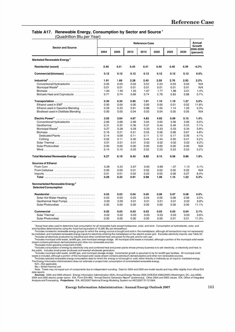
7/28/2019 2007 Annual Energy Outlook
http://slidepdf.com/reader/full/2007-annual-energy-outlook 172/243
Energy Information Administration / Annual Energy Outlook 2007 163
Reference Case
Table A17. Renewable Energy, Consumption by Sector and Source1
(Quadrillion Btu per Year)
Sector and Source
Reference Case AnnualGrowth
2005-2030(percent)2004 2005 2010 2015 2020 2025 2030
Marketed Renewable Energy2
Residential (wood) . . . . . . . . . . . . . . . . . . . . . . 0.40 0.41 0.43 0.41 0.40 0.40 0.39 -0.2%
Commercial (biomass) . . . . . . . . . . . . . . . . . . . 0.12 0.12 0.12 0.12 0.12 0.12 0.12 0.0%
Industrial3 . . . . . . . . . . . . . . . . . . . . . . . . . . . . . . 1.91 1.69 2.28 2.45 2.59 2.76 2.93 2.2%
Conventional Hydroelectric . . . . . . . . . . . . . . . 0.05 0.03 0.03 0.03 0.03 0.03 0.03 N/A
Municipal Waste4 . . . . . . . . . . . . . . . . . . . . . . . 0.01 0.01 0.01 0.01 0.01 0.01 0.01 N/A
Biomass . . . . . . . . . . . . . . . . . . . . . . . . . . . . . . 1.64 1.40 1.55 1.67 1.77 1.88 2.01 1.4%
Biofuels Heat and Coproducts . . . . . . . . . . . . . 0.21 0.24 0.69 0.74 0.78 0.83 0.88 5.2%
Transportation . . . . . . . . . . . . . . . . . . . . . . . . . . 0.30 0.34 0.95 1.01 1.10 1.19 1.27 5.5%
Ethanol used in E855 . . . . . . . . . . . . . . . . . . . . 0.00 0.00 0.00 0.00 0.00 0.01 0.02 11.8%
Ethanol used in Gasoline Blending . . . . . . . . . 0.29 0.33 0.91 0.98 1.05 1.14 1.20 5.3%
Biodiesel used in Distillate Blending . . . . . . . . 0.00 0.00 0.04 0.03 0.04 0.05 0.05 N/A
Electric Power6 . . . . . . . . . . . . . . . . . . . . . . . . . 3.55 3.64 4.67 4.83 4.93 5.09 5.15 1.4%
Conventional Hydroelectric . . . . . . . . . . . . . . . 2.66 2.68 2.99 3.04 3.05 3.06 3.06 0.5%
Geothermal . . . . . . . . . . . . . . . . . . . . . . . . . . . . 0.31 0.32 0.36 0.37 0.44 0.48 0.53 2.1%
Municipal Waste7 . . . . . . . . . . . . . . . . . . . . . . . 0.27 0.28 0.29 0.33 0.33 0.33 0.34 0.8%
Biomass . . . . . . . . . . . . . . . . . . . . . . . . . . . . . . 0.16 0.21 0.51 0.55 0.56 0.68 0.67 4.8%
Dedicated Plants . . . . . . . . . . . . . . . . . . . . . . 0.14 0.09 0.11 0.11 0.12 0.17 0.26 4.1%
Cofiring . . . . . . . . . . . . . . . . . . . . . . . . . . . . . 0.02 0.11 0.40 0.44 0.44 0.50 0.41 5.2%
Solar Thermal . . . . . . . . . . . . . . . . . . . . . . . . . . 0.01 0.01 0.01 0.02 0.02 0.02 0.02 6.2%
Solar Photovoltaic . . . . . . . . . . . . . . . . . . . . . . 0.00 0.00 0.00 0.00 0.00 0.00 0.00 N/A
Wind . . . . . . . . . . . . . . . . . . . . . . . . . . . . . . . . . 0.14 0.15 0.50 0.52 0.53 0.53 0.53 5.2%
Total Marketed Renewable Energy . . . . . . . . . . . 6.27 6.19 8.45 8.82 9.15 9.56 9.86 1.9%
Sources of Ethanol
From Corn . . . . . . . . . . . . . . . . . . . . . . . . . . . . . . 0.28 0.33 0.87 0.93 0.99 1.07 1.13 5.1%
From Cellulose . . . . . . . . . . . . . . . . . . . . . . . . . . 0.00 0.00 0.01 0.02 0.02 0.02 0.02 N/A
Imports . . . . . . . . . . . . . . . . . . . . . . . . . . . . . . . . 0.01 0.01 0.02 0.03 0.05 0.06 0.07 8.4%Total . . . . . . . . . . . . . . . . . . . . . . . . . . . . . . . . . 0.29 0.33 0.91 0.98 1.06 1.15 1.22 5.3%
Nonmarketed Renewable Energy8
Selected Consumption
Residential . . . . . . . . . . . . . . . . . . . . . . . . . . . . . 0.03 0.03 0.04 0.05 0.06 0.07 0.08 4.0%
Solar Hot Water Heating . . . . . . . . . . . . . . . . . 0.03 0.03 0.03 0.04 0.05 0.06 0.06 3.5%
Geothermal Heat Pumps . . . . . . . . . . . . . . . . . 0.00 0.00 0.01 0.01 0.01 0.01 0.02 6.8%
Solar Photovoltaic . . . . . . . . . . . . . . . . . . . . . . 0.00 0.00 0.00 0.00 0.00 0.00 0.00 11.1%
Commercial . . . . . . . . . . . . . . . . . . . . . . . . . . . . 0.02 0.03 0.03 0.03 0.03 0.03 0.04 2.1%
Solar Thermal . . . . . . . . . . . . . . . . . . . . . . . . . . 0.02 0.02 0.03 0.03 0.03 0.03 0.03 0.6%
Solar Photovoltaic . . . . . . . . . . . . . . . . . . . . . . 0.00 0.00 0.00 0.00 0.00 0.01 0.01 11.3%
1Actual heat rates used to determine fuel consumption for all renewable fuels except hydropower, solar, and wind. Consumption at hydroelectric, solar, andwind facilities determined by using the fossil fuel equivalent of 10,280 Btu per kilowatthour.
2Includes nonelectric renewable energy groups for which the energy source is bought and sold in the marketplace, although all transactions may not necessarilybe marketed, and marketed renewable energy inputs for electricity entering the marketplace on the electric power grid. Excludes electricity imports; see Table A2.
3Includes all electricity production by industrial and other combined heat and power for the grid and for own use.4Includes municipal solid waste, landfill gas, and municipal sewage sludge. All municipal solid waste is included, although a portion of the municipal solid waste
stream contains petroleum-derived plastics and other non-renewable sources.5Excludes motor gasoline component of E85.6Includes consumption of energy by electricity-only and combined heat and power plants whose primary business is to sell electricity, or electricity and heat, to
the public. Includes small power producers and exempt wholesale generators.7Includes municipal solid waste, landfill gas, and municipal sewage sludge. Incremental growth is assumed to be for landfill gas facilities. All municipal solid
waste is included, although a portion of the municipal solid waste stream contains petroleum-derived plastics and other non-renewable sources.8Includes selected renewable energy consumption data for which the energy is not bought or sold, either directly or indirectly as an input to marketed energy.
The Energy Information Administration does not estimate or project total consumption of nonmarketed renewable energy.N/A = Not applicable.Btu = British thermal unit.Note: Totals may not equal sum of components due to independent rounding. Data for 2004 and 2005 are model results and may differ slightly from official EIA
data reports.Sources: 2004 and 2005 ethanol: Energy Information Administration (EIA), Annual Energy Review 2005 , DOE/EIA-0384(2005) (Washington, DC, July 2006).
2004 and 2005 electric power sector: EIA, Form EIA-860, "Annual Electric Generator Report” (preliminary). Other 2004 and 2005 values: EIA, Office of IntegratedAnalysis and Forecasting. Projections: EIA, AEO2007 National Energy Modeling System run AEO2007.D112106A.

7/28/2019 2007 Annual Energy Outlook
http://slidepdf.com/reader/full/2007-annual-energy-outlook 173/243
164 Energy Information Administration / Annual Energy Outlook 2007
Reference Case
Table A18. Carbon Dioxide Emissions by Sector and Source(Million Metric Tons, Unless Otherwise Noted)
Sector and Source
Reference Case AnnualGrowth
2005-2030(percent)2004 2005 2010 2015 2020 2025 2030
Residential
Petroleum . . . . . . . . . . . . . . . . . . . . . . . . . . . . . . 106 105 105 107 105 102 100 -0.2%
Natural Gas . . . . . . . . . . . . . . . . . . . . . . . . . . . . . 265 262 274 282 287 288 289 0.4%
Coal . . . . . . . . . . . . . . . . . . . . . . . . . . . . . . . . . . . 1 1 1 1 1 1 1 -0.2%
Electricity1 . . . . . . . . . . . . . . . . . . . . . . . . . . . . . . 842 886 940 1002 1064 1143 1225 1.3%
Total . . . . . . . . . . . . . . . . . . . . . . . . . . . . . . . . . 1214 1254 1320 1392 1456 1534 1614 1.0%
Commercial
Petroleum . . . . . . . . . . . . . . . . . . . . . . . . . . . . . . 54 55 54 57 57 58 59 0.2%
Natural Gas . . . . . . . . . . . . . . . . . . . . . . . . . . . . . 170 166 175 192 204 216 230 1.3%
Coal . . . . . . . . . . . . . . . . . . . . . . . . . . . . . . . . . . . 10 8 9 9 9 9 9 0.6%
Electricity1 . . . . . . . . . . . . . . . . . . . . . . . . . . . . . . 800 822 886 975 1059 1185 1332 1.9%
Total . . . . . . . . . . . . . . . . . . . . . . . . . . . . . . . . . 1034 1051 1124 1233 1330 1469 1630 1.8%
Industrial2
Petroleum . . . . . . . . . . . . . . . . . . . . . . . . . . . . . . 437 431 406 419 423 433 457 0.2%
Natural Gas3
. . . . . . . . . . . . . . . . . . . . . . . . . . . . 435 400 466 468 493 513 524 1.1%Coal . . . . . . . . . . . . . . . . . . . . . . . . . . . . . . . . . . . 201 189 186 194 199 243 269 1.4%
Electricity1 . . . . . . . . . . . . . . . . . . . . . . . . . . . . . . 663 663 674 694 702 734 774 0.6%
Total . . . . . . . . . . . . . . . . . . . . . . . . . . . . . . . . . 1736 1682 1732 1775 1817 1924 2024 0.7%
Transportation
Petroleum4 . . . . . . . . . . . . . . . . . . . . . . . . . . . . . . 1902 1922 1994 2142 2288 2443 2626 1.3%
Natural Gas5 . . . . . . . . . . . . . . . . . . . . . . . . . . . . 32 32 38 41 47 48 48 1.7%
Electricity1 . . . . . . . . . . . . . . . . . . . . . . . . . . . . . . 5 5 5 6 6 7 7 1.8%
Total . . . . . . . . . . . . . . . . . . . . . . . . . . . . . . . . . 1939 1958 2037 2189 2341 2498 2682 1.3%
Electric Power6
Petroleum . . . . . . . . . . . . . . . . . . . . . . . . . . . . . . 98 100 69 75 74 76 77 -1.1%
Natural Gas . . . . . . . . . . . . . . . . . . . . . . . . . . . . . 296 319 346 385 390 357 321 0.0%
Coal . . . . . . . . . . . . . . . . . . . . . . . . . . . . . . . . . . . 1904 1944 2078 2203 2354 2623 2927 1.6%
Other7 . . . . . . . . . . . . . . . . . . . . . . . . . . . . . . . . . 11 12 12 14 14 14 14 0.8%
Total . . . . . . . . . . . . . . . . . . . . . . . . . . . . . . . . . 2309 2375 2505 2677 2832 3070 3338 1.4%
Total by Fuel
Petroleum3 . . . . . . . . . . . . . . . . . . . . . . . . . . . . . . 2598 2614 2629 2799 2947 3112 3318 1.0%
Natural Gas . . . . . . . . . . . . . . . . . . . . . . . . . . . . . 1198 1178 1298 1369 1420 1422 1412 0.7%
Coal . . . . . . . . . . . . . . . . . . . . . . . . . . . . . . . . . . . 2115 2142 2275 2407 2563 2877 3206 1.6%
Other7 . . . . . . . . . . . . . . . . . . . . . . . . . . . . . . . . . 11 12 12 14 14 14 14 0.8%
Total . . . . . . . . . . . . . . . . . . . . . . . . . . . . . . . . . 5923 5945 6214 6589 6944 7425 7950 1.2%
Carbon Dioxide Emissions
(tons per person) . . . . . . . . . . . . . . . . . . . . . . . . . 20.1 20.0 20.0 20.4 20.6 21.2 21.8 0.3%
1Emissions from the electric power sector are distributed to the end-use sectors.2Fuel consumption includes energy for combined heat and power plants (CHP), except those plants whose primary business is to sell electricity, or electricity
and heat, to the public.3Includes lease and plant fuel.4This includes carbon dioxide from international bunker fuels, both civilian and military, which are excluded from the accounting of carbon dioxide emissions
under the United Nations convention. From 1990 through 2004, international bunker fuels accounted for 83 to 115 million metric tons annually.5Includes pipeline fuel natural gas and compressed natural gas used as vehicle fuel.6Includes electricity-only and combined heat and power plants whose primary business is to sell electricity, or electricity and heat, to the public.7Includes emissions from geothermal power and nonbiogenic emissions from municipal solid waste.Note: Totals may not equal sum of components due to independent rounding. Data for 2004 and 2005 are model results and may differ slightly from official EIA
data reports.Sources: 2004 and 2005 emissions and emission factors: Energy Information Administration (EIA), Emissions of Greenhouse Gases in the United States
2005, DOE/EIA-0573(2005) (Washington, DC, November 2006). Projections: EIA, AEO2007 National Energy Modeling System run AEO2007.D112106A.

7/28/2019 2007 Annual Energy Outlook
http://slidepdf.com/reader/full/2007-annual-energy-outlook 174/243
Energy Information Administration / Annual Energy Outlook 2007 165
Reference Case
Table A19. Macroeconomic Indicators(Billion 2000 Chain-Weighted Dollars, Unless Otherwise Noted)
Indicators
Reference Case AnnualGrowth
2005-2030(percent)2004 2005 2010 2015 2020 2025 2030
Real Gross Domestic Product . . . . . . . . . . . . . 10704 11049 12790 14698 17077 19666 22494 2.9%
Components of Real Gross Domestic Product
Real Consumption . . . . . . . . . . . . . . . . . . . . . . . 7577 7841 9111 10423 12006 13731 15590 2.8%
Real Investment . . . . . . . . . . . . . . . . . . . . . . . . 1771 1866 2139 2478 3030 3773 4735 3.8%
Real Government Spending . . . . . . . . . . . . . . . 1941 1958 2117 2242 2396 2541 2709 1.3%
Real Exports . . . . . . . . . . . . . . . . . . . . . . . . . . . 1120 1196 1767 2543 3584 4894 6581 7.1%
Real Imports . . . . . . . . . . . . . . . . . . . . . . . . . . . 1711 1815 2321 2911 3761 4963 6649 5.3%
Energy Intensity
(thousand Btu per 2000 dollar of GDP)
Delivered Energy . . . . . . . . . . . . . . . . . . . . . . . . 6.91 6.60 6.06 5.56 5.04 4.62 4.27 -1.7%
Total Energy . . . . . . . . . . . . . . . . . . . . . . . . . . . 9.41 9.07 8.33 7.64 6.92 6.33 5.83 -1.8%
Price Indices
GDP Chain-type Price Index (2000=1.000) . . . 1.094 1.127 1.253 1.366 1.495 1.648 1.815 1.9%
Consumer Price Index (1982-4=1.00)
All-urban . . . . . . . . . . . . . . . . . . . . . . . . . . . . . 1.89 1.95 2.16 2.36 2.61 2.90 3.23 2.0%Energy Commodities and Services . . . . . . . . 1.51 1.77 1.93 1.94 2.19 2.48 2.80 1.8%
Wholesale Price Index (1982=1.00)
All Commodities . . . . . . . . . . . . . . . . . . . . . . . 1.47 1.57 1.68 1.72 1.82 1.94 2.06 1.1%
Fuel and Power . . . . . . . . . . . . . . . . . . . . . . . 1.27 1.57 1.64 1.62 1.84 2.11 2.39 1.7%
Interest Rates (percent, nominal)
Federal Funds Rate . . . . . . . . . . . . . . . . . . . . . . 1.35 3.21 4.71 4.93 5.11 5.07 5.14 N/A
10-Year Treasury Note . . . . . . . . . . . . . . . . . . . 4.27 4.29 5.52 5.66 5.75 5.78 5.80 N/A
AA Utility Bond Rate . . . . . . . . . . . . . . . . . . . . . 6.04 5.44 7.36 7.64 7.72 7.78 7.77 N/A
Value of Shipments (billion 2000 dollars)
Total Industrial . . . . . . . . . . . . . . . . . . . . . . . . . . 5651 5763 6298 7033 7779 8585 9502 2.0%
Nonmanufacturing . . . . . . . . . . . . . . . . . . . . . 1494 1538 1596 1701 1846 1940 2023 1.1%
Manufacturing . . . . . . . . . . . . . . . . . . . . . . . . . 4157 4225 4702 5332 5933 6645 7478 2.3%
Energy-Intensive . . . . . . . . . . . . . . . . . . . . . 1161 1160 1262 1347 1426 1522 1631 1.4%
Non-energy Intensive . . . . . . . . . . . . . . . . . 2996 3065 3440 3985 4507 5123 5848 2.6%
Population and Employment (millions)
Population, with Armed Forces Overseas . . . . . 294.2 296.9 310.3 323.7 337.1 350.8 364.9 0.8%
Population, aged 16 and over . . . . . . . . . . . . . . 229.2 231.8 244.2 254.7 265.4 276.7 288.6 0.9%
Population, over age 65 . . . . . . . . . . . . . . . . . . 36.4 36.8 40.4 47.0 54.9 63.8 71.6 2.7%
Employment, Nonfarm . . . . . . . . . . . . . . . . . . . . 131.4 133.4 141.9 147.0 154.6 162.3 169.2 1.0%
Employment, Manufacturing . . . . . . . . . . . . . . . 14.3 14.2 13.8 13.7 13.4 13.0 12.5 -0.5%
Key Labor Indicators
Labor Force (millions) . . . . . . . . . . . . . . . . . . . . 147.4 149.3 157.5 162.2 167.0 172.7 180.4 0.8%
Nonfarm Labor Productivity (1992=1.00) . . . . . 1.32 1.36 1.50 1.69 1.90 2.15 2.42 2.3%
Unemployment Rate (percent) . . . . . . . . . . . . . 5.52 5.06 4.83 4.98 4.46 4.55 4.71 N/A
Key Indicators for Energy Demand
Real Disposable Personal Income . . . . . . . . . . 8011 8105 9568 11077 13000 15172 17535 3.1%
Housing Starts (millions) . . . . . . . . . . . . . . . . . . 2.08 2.22 1.94 1.91 1.90 1.85 1.80 -0.8%
Commercial Floorspace (billion square feet) . . . 73.0 74.3 80.4 86.5 92.9 100.1 108.0 1.5%
Unit Sales of Light-Duty Vehicles (millions) . . . 16.87 16.95 17.14 18.05 19.04 20.01 21.10 0.9%
GDP = Gross domestic product.Btu = British thermal unit.N/A = Not applicable.Sources: 2004 and 2005: Global Insight macroeconomic model CTL0806 and Global Insight industry model, July 2005. Projections: Energy Information
Administration, AEO2007 National Energy Modeling System run AEO2007.D112106A.

7/28/2019 2007 Annual Energy Outlook
http://slidepdf.com/reader/full/2007-annual-energy-outlook 175/243
166 Energy Information Administration / Annual Energy Outlook 2007
Reference Case
Table A20. International Petroleum Supply and Disposition Summary(Million Barrels per Day, Unless Otherwise Noted)
Supply and Disposition
Reference Case AnnualGrowth
2005-2030(percent)2004 2005 2010 2015 2020 2025 2030
Crude Oil Prices (2005 dollars per barrel)1
Imported Low Sulfur Light Crude Oil . . . . . . . . . . 42.87 56.76 57.47 49.87 52.04 56.37 59.12 0.2%
Imported Crude Oil . . . . . . . . . . . . . . . . . . . . . . . 37.09 49.19 51.20 44.61 46.47 49.57 51.63 0.2%
Conventional Production (Conventional)2
OPEC3
Asia . . . . . . . . . . . . . . . . . . . . . . . . . . . . . . . . 1.18 1.17 1.11 1.10 1.09 1.08 1.10 -0.2%
Middle East . . . . . . . . . . . . . . . . . . . . . . . . . . 22.60 22.96 22.23 24.03 26.60 29.72 33.20 1.5%
North Africa . . . . . . . . . . . . . . . . . . . . . . . . . . 3.55 3.78 4.29 4.51 4.24 4.07 3.93 0.2%
West Africa . . . . . . . . . . . . . . . . . . . . . . . . . . 2.47 2.78 3.07 3.81 4.10 4.32 4.48 1.9%
South America . . . . . . . . . . . . . . . . . . . . . . . . 2.75 2.71 2.59 2.42 2.30 2.24 2.24 -0.8%
Total OPEC . . . . . . . . . . . . . . . . . . . . . . . . 32.55 33.41 33.30 35.87 38.33 41.44 44.95 1.2%
Non-OPEC
OECD
United States (50 states) . . . . . . . . . . . . . . . . 8.46 8.03 8.98 9.45 9.48 9.18 9.12 0.5%
Canada . . . . . . . . . . . . . . . . . . . . . . . . . . . . . 2.12 2.12 1.93 2.01 1.89 1.76 1.62 -1.1%
Mexico . . . . . . . . . . . . . . . . . . . . . . . . . . . . . . 3.85 3.78 3.15 3.01 3.18 3.35 3.52 -0.3%OECD Europe4 . . . . . . . . . . . . . . . . . . . . . . . 6.39 5.96 5.73 4.91 4.22 3.64 3.16 -2.5%
Japan . . . . . . . . . . . . . . . . . . . . . . . . . . . . . . . 0.12 0.10 0.10 0.10 0.10 0.10 0.10 0.0%
Australia and New Zealand . . . . . . . . . . . . . . 0.58 0.60 0.56 0.51 0.51 0.55 0.60 -0.0%
Total OECD . . . . . . . . . . . . . . . . . . . . . . . . 21.53 20.59 20.45 20.00 19.39 18.57 18.12 -0.5%
Non-OECD
Russia . . . . . . . . . . . . . . . . . . . . . . . . . . . . . . 9.27 9.51 9.98 10.30 10.79 11.23 11.54 0.8%
Other Eurasia5 . . . . . . . . . . . . . . . . . . . . . . . . 2.21 2.48 3.98 4.91 5.41 5.99 6.55 4.0%
China . . . . . . . . . . . . . . . . . . . . . . . . . . . . . . . 3.64 3.74 3.53 3.20 3.30 3.30 3.20 -0.6%
Other Asia6 . . . . . . . . . . . . . . . . . . . . . . . . . . 2.80 2.53 2.29 2.50 2.60 2.60 2.50 -0.1%
Middle East7 . . . . . . . . . . . . . . . . . . . . . . . . . 1.68 1.67 2.00 2.20 2.40 2.70 2.90 2.2%
Africa . . . . . . . . . . . . . . . . . . . . . . . . . . . . . . . 3.40 3.59 5.19 6.45 7.38 8.51 9.83 4.1%
Brazil . . . . . . . . . . . . . . . . . . . . . . . . . . . . . . . 1.58 1.76 2.39 2.90 3.20 3.50 3.90 3.2%
Other Central and South America . . . . . . . . . 2.35 2.31 2.32 2.54 2.66 2.75 2.90 0.9%
Total Non-OECD . . . . . . . . . . . . . . . . . . . . 26.94 27.59 31.67 35.00 37.75 40.59 43.32 1.8%
Total Conventional Production . . . . . . . . . . . . . . 81.01 81.59 85.42 90.86 95.47 100.59 106.40 1.1%
Unconventional Production8
United States (50 states) . . . . . . . . . . . . . . . . . . . 0.22 0.25 0.71 0.81 0.91 1.20 1.37 7.0%
Other North America . . . . . . . . . . . . . . . . . . . . . . 1.09 1.09 1.91 2.32 2.74 3.25 3.66 5.0%
OECD Europe3 . . . . . . . . . . . . . . . . . . . . . . . . . . 0.04 0.08 0.15 0.18 0.19 0.23 0.27 5.1%
Middle East7 . . . . . . . . . . . . . . . . . . . . . . . . . . . . 0.08 0.02 0.57 0.64 0.75 0.89 1.11 16.8%
Africa. . . . . . . . . . . . . . . . . . . . . . . . . . . . . . . . . . 0.16 0.16 0.32 0.42 0.52 0.62 0.73 6.3%
Central and South America . . . . . . . . . . . . . . . . . 0.83 0.93 1.35 1.59 1.81 2.18 2.40 3.9%
Other . . . . . . . . . . . . . . . . . . . . . . . . . . . . . . . . . . 0.02 0.28 0.62 0.81 0.90 1.05 1.41 6.7%
Total Unconventional Production . . . . . . . . . 2.44 2.80 5.63 6.78 7.83 9.42 10.93 5.6%
Total Production . . . . . . . . . . . . . . . . . . . . . . . . . . 83.45 84.39 91.05 97.64 103.29 110.01 117.33 1.3%

7/28/2019 2007 Annual Energy Outlook
http://slidepdf.com/reader/full/2007-annual-energy-outlook 176/243
Energy Information Administration / Annual Energy Outlook 2007 167
Reference Case
Table A20. International Petroleum Supply and Disposition Summary (Continued)(Million Barrels per Day, Unless Otherwise Noted)
Supply and Disposition
Reference Case AnnualGrowth
2005-2030(percent)2004 2005 2010 2015 2020 2025 2030
Consumption9
OECD
United States (50 states) . . . . . . . . . . . . . . . . . 20.76 20.75 21.59 22.85 24.02 25.33 26.93 1.0%
United States Territories . . . . . . . . . . . . . . . . . . 0.37 0.38 0.43 0.47 0.51 0.54 0.59 1.8%
Canada . . . . . . . . . . . . . . . . . . . . . . . . . . . . . . . 2.32 2.28 2.42 2.54 2.49 2.56 2.59 0.5%
Mexico . . . . . . . . . . . . . . . . . . . . . . . . . . . . . . . 2.00 2.09 2.22 2.47 2.68 2.93 3.19 1.7%
OECD Europe3 . . . . . . . . . . . . . . . . . . . . . . . . . 15.86 15.73 15.82 15.89 15.76 16.00 16.26 0.1%
Japan . . . . . . . . . . . . . . . . . . . . . . . . . . . . . . . . 5.43 5.58 5.42 5.48 5.43 5.46 5.45 -0.1%
South Korea . . . . . . . . . . . . . . . . . . . . . . . . . . . 2.18 2.30 2.58 2.85 3.04 3.24 3.45 1.6%
Australia and New Zealand . . . . . . . . . . . . . . . 1.04 1.05 1.08 1.10 1.13 1.17 1.22 0.6%
Total OECD . . . . . . . . . . . . . . . . . . . . . . . . . 49.95 50.16 51.54 53.65 55.05 57.25 59.69 0.7%
Non-OECD
Russia . . . . . . . . . . . . . . . . . . . . . . . . . . . . . . . 2.81 2.75 2.85 3.05 3.11 3.28 3.39 0.8%
Other Non-OECD Eurasia5 . . . . . . . . . . . . . . . . 2.03 2.33 2.63 2.95 3.18 3.46 3.75 1.9%
China . . . . . . . . . . . . . . . . . . . . . . . . . . . . . . . . 6.49 6.86 8.70 9.99 11.66 13.24 15.05 3.2%
India . . . . . . . . . . . . . . . . . . . . . . . . . . . . . . . . . 2.48 2.52 2.94 3.32 3.66 4.07 4.45 2.3%Other Non-OECD Asia . . . . . . . . . . . . . . . . . . . 6.03 6.02 6.89 7.70 8.51 9.36 10.29 2.2%
Middle East7 . . . . . . . . . . . . . . . . . . . . . . . . . . . 5.74 5.56 6.06 6.60 7.00 7.43 7.81 1.4%
Africa . . . . . . . . . . . . . . . . . . . . . . . . . . . . . . . . 2.83 3.01 3.70 4.05 4.30 4.54 4.93 2.0%
Brazil . . . . . . . . . . . . . . . . . . . . . . . . . . . . . . . . 2.17 2.20 2.39 2.63 2.82 3.09 3.29 1.6%
Other Central and South America . . . . . . . . . . 2.94 2.99 3.36 3.71 4.00 4.29 4.68 1.8%
Total Non-OECD . . . . . . . . . . . . . . . . . . . . . 33.50 34.23 39.52 44.00 48.23 52.76 57.64 2.1%
Total Consumption . . . . . . . . . . . . . . . . . . . . . . . . 83.45 84.39 91.05 97.64 103.29 110.01 117.33 1.3%
OPEC Production10 . . . . . . . . . . . . . . . . . . . . . . . . . 33.20 34.04 34.72 37.47 40.19 43.71 47.65 1.4%
Non-OPEC Production10 . . . . . . . . . . . . . . . . . . . . . 50.25 50.35 56.34 60.18 63.10 66.30 69.68 1.3%
Net Eurasia Exports . . . . . . . . . . . . . . . . . . . . . . . . 8.24 8.67 10.87 12.10 13.12 13.98 14.85 2.2%
OPEC Market Share . . . . . . . . . . . . . . . . . . . . . . . . 39.8 40.3 38.1 38.4 38.9 39.7 40.6 0.0%
1Weighted average price delivered to U.S. refiners.2Includes production of crude oil (including lease condensates), natural gas plant liquids, other hydrogen and hydrocarbons for refinery feedstocks, alcohol and
other sources, and refinery gains.3OPEC = Organization of Petroleum Exporting Countries - Algeria, Indonesia, Iran, Iraq, Kuwait, Libya, Nigeria, Qatar, Saudi Arabia, the United Arab Emirates,and Venezuela. Does not include Angola, which was admitted as a full member to OPEC on December 14, 2006.
4OECD Europe = Organization for Economic Cooperation and Development - Austria, Belgium, Czech Republic, Denmark, Finland, France, Germany, Greece,Hungary, Iceland, Ireland, Italy, Luxembourg, the Netherlands, Norway, Poland, Portugal, Slovakia, Spain, Sweden, Switzerland, Turkey, and the United Kingdom.
5Eurasia consists of Armenia, Azerbaijan, Belarus, Estonia, Georgia, Kazakhstan, Kyrgyzstan, Latvia, Lithuania, Moldova, Russia, Tajikistan, Turkmenistan,Ukraine, and Uzbekistan.
6Other Asia = Afghanistan, Bangladesh, Bhutan, Brunei, Cambodia (Kampuchea), Fiji, French Polynesia, Guam, Hong Kong, Indonesia, Kiribati, Laos, Malaysia,Macau, Maldives, Mongolia, Myanmar (Burma), Nauru, Nepal, New Caledonia, Niue, North Korea, Pakistan, Papua New Guinea, Philippines, Samoa, Singapore,Solomon Islands, Sri Lanka, Taiwan, Thailand, Tonga, Vanuatu, and Vietnam.
7Non-OPEC Middle East includes Turkey.8Includes liquids produced from energy crops, natural gas, coal, oil sands, and shale. Includes both OPEC and non-OPEC producers in the regional
breakdown.9Includes both OPEC and non-OPEC consumers in the regional breakdown.10Includes both conventional and nonconventional liquids production.Note: Totals may not equal sum of components due to independent rounding. Data for 2004 and 2005 are model results and may differ slightly from official EIA
data reports.Sources: 2004 and 2005 low sulfur light crude oil price: Energy Information Administration (EIA), Form EIA-856, “Monthly Foreign Crude Oil Acquisition
Report.” 2004 and 2005 imported crude oil price: EIA, Annual Energy Review 2005 , DOE/EIA-0384(2005) (Washington, DC, July 2006). 2004 quantities derivedfrom: EIA, International Energy Annual 2004 , DOE/EIA-0219(2004) (Washington, DC, May-July 2006). 2005 quantities and projections: EIA, AEO2007National Energy Modeling System run AEO2007.D112106A.

7/28/2019 2007 Annual Energy Outlook
http://slidepdf.com/reader/full/2007-annual-energy-outlook 177/243

7/28/2019 2007 Annual Energy Outlook
http://slidepdf.com/reader/full/2007-annual-energy-outlook 178/243
Energy Information Administration / Annual Energy Outlook 2007 169
Appendix B
Economic Growth Case Comparisons
Table B1. Total Energy Supply and Disposition Summary(Quadrillion Btu per Year, Unless Otherwise Noted)
Supply, Disposition, and Prices 2005
Projections
2010 2020 2030
LowEconomic
GrowthReference
HighEconomic
Growth
LowEconomic
GrowthReference
HighEconomic
Growth
LowEconomic
GrowthReference
HighEconomic
Growth
Production
Crude Oil and Lease Condensate . . . . . . . . . . 10.96 11.98 11.99 12.01 12.25 12.48 12.65 11.25 11.40 11.53
Natural Gas Plant Liquids . . . . . . . . . . . . . . . . 2.33 2.39 2.43 2.46 2.30 2.38 2.42 2.22 2.31 2.39
Dry Natural Gas . . . . . . . . . . . . . . . . . . . . . . . . 18.77 19.61 19.93 20.19 20.81 21.41 21.80 20.36 21.15 21.88
Coal1 . . . . . . . . . . . . . . . . . . . . . . . . . . . . . . . . 23.20 24.36 24.47 24.58 25.19 26.61 28.22 29.64 33.52 36.90
Nuclear Power . . . . . . . . . . . . . . . . . . . . . . . . . 8.13 8.23 8.23 8.23 8.91 9.23 9.28 8.80 9.33 10.53
Hydropower . . . . . . . . . . . . . . . . . . . . . . . . . . . 2.71 3.02 3.02 3.02 3.09 3.08 3.08 3.09 3.09 3.10
Biomass2 . . . . . . . . . . . . . . . . . . . . . . . . . . . . . 2.71 4.15 4.22 4.32 4.47 4.69 5.04 4.66 5.26 6.06
Other Renewable Energy3 . . . . . . . . . . . . . . . . 0.76 1.20 1.18 1.18 1.28 1.33 1.32 1.38 1.44 1.51
Other4 . . . . . . . . . . . . . . . . . . . . . . . . . . . . . . . 0.22 0.66 0.67 0.73 0.90 0.89 1.09 0.99 1.12 1.21
Total . . . . . . . . . . . . . . . . . . . . . . . . . . . . . . . 69.80 75.60 76.13 76.71 79.20 82.09 84.91 82.37 88.63 95.10
Imports
Crude Oil5 . . . . . . . . . . . . . . . . . . . . . . . . . . . . 22.09 21.39 21.88 22.55 23.16 24.72 26.54 25.19 28.63 33.17Liquid Fuels and Other Petroleum6 . . . . . . . . . 7.16 5.64 6.02 6.27 6.30 7.05 7.80 7.27 9.02 10.13
Natural Gas . . . . . . . . . . . . . . . . . . . . . . . . . . . 4.42 5.12 5.36 5.59 5.63 6.17 6.80 5.41 6.47 8.03
Other Imports7 . . . . . . . . . . . . . . . . . . . . . . . . . 0.85 0.92 0.92 0.94 1.66 1.73 1.81 2.03 2.26 2.16
Total . . . . . . . . . . . . . . . . . . . . . . . . . . . . . . . 34.52 33.07 34.18 35.34 36.75 39.66 42.96 39.89 46.37 53.49
Exports
Petroleum8 . . . . . . . . . . . . . . . . . . . . . . . . . . . . 2.31 2.69 2.71 2.75 2.78 2.84 2.92 2.80 2.90 3.03
Natural Gas . . . . . . . . . . . . . . . . . . . . . . . . . . . 0.75 0.70 0.69 0.68 0.72 0.69 0.66 0.95 0.87 0.78
Coal . . . . . . . . . . . . . . . . . . . . . . . . . . . . . . . . . 1.27 1.12 1.12 1.12 0.88 0.80 0.74 0.66 0.69 0.67
Total . . . . . . . . . . . . . . . . . . . . . . . . . . . . . . . 4.33 4.50 4.52 4.55 4.38 4.33 4.31 4.41 4.47 4.49
Discrepancy9 . . . . . . . . . . . . . . . . . . . . . . . . . . . -0.20 -0.66 -0.70 -0.71 -0.60 -0.74 -0.60 -0.64 -0.63 -0.30
Consumption
Liquid Fuels and Other Petroleum10 . . . . . . . . 40.61 40.80 41.76 42.78 43.72 46.52 49.44 46.52 52.17 57.99
Natural Gas . . . . . . . . . . . . . . . . . . . . . . . . . . . 22.63 24.17 24.73 25.23 25.86 27.04 28.10 24.94 26.89 29.28
Coal . . . . . . . . . . . . . . . . . . . . . . . . . . . . . . . . . 22.87 24.13 24.24 24.35 25.80 27.29 28.97 30.16 34.14 37.29Nuclear Power . . . . . . . . . . . . . . . . . . . . . . . . . 8.13 8.23 8.23 8.23 8.91 9.23 9.28 8.80 9.33 10.53
Hydropower . . . . . . . . . . . . . . . . . . . . . . . . . . . 2.71 3.02 3.02 3.02 3.09 3.08 3.08 3.09 3.09 3.10
Biomass11 . . . . . . . . . . . . . . . . . . . . . . . . . . . . 2.38 3.24 3.30 3.38 3.47 3.64 3.91 3.56 4.06 4.66
Other Renewable Energy3 . . . . . . . . . . . . . . . . 0.76 1.20 1.18 1.18 1.28 1.33 1.32 1.38 1.44 1.51
Other12 . . . . . . . . . . . . . . . . . . . . . . . . . . . . . . . 0.08 0.04 0.04 0.05 0.04 0.04 0.04 0.04 0.04 0.05
Total . . . . . . . . . . . . . . . . . . . . . . . . . . . . . . . 100.19 104.83 106.50 108.21 112.16 118.16 124.14 118.50 131.16 144.40

7/28/2019 2007 Annual Energy Outlook
http://slidepdf.com/reader/full/2007-annual-energy-outlook 179/243
170 Energy Information Administration / Annual Energy Outlook 2007
Economic Growth Case Comparisons
Table B1. Total Energy Supply and Disposition Summary (Continued)(Quadrillion Btu per Year, Unless Otherwise Noted)
Supply, Disposit ion, and Prices 2005
Projections
2010 2020 2030
LowEconomic
Growth
ReferenceHigh
Economic
Growth
LowEconomic
Growth
ReferenceHigh
Economic
Growth
LowEconomic
Growth
ReferenceHigh
Economic
Growth
Prices (2005 dollars per unit)
Petroleum (dollars per barrel)
Imported Low Sulfur Light Crude Oil Price13 56.76 57.47 57.47 57.13 52.51 52.04 52.04 59.12 59.12 59.12
Imported Crude Oil Price13 . . . . . . . . . . . . . . 49.19 51.20 51.20 51.20 46.47 46.47 46.47 51.63 51.63 51.63
Natural Gas (dollars per million Btu)
Price at Henry Hub . . . . . . . . . . . . . . . . . . . . 8.60 6.05 6.28 6.50 5.41 5.71 5.73 6.16 6.52 6.87
Wellhead Price14 . . . . . . . . . . . . . . . . . . . . . . 7.29 5.38 5.59 5.79 4.80 5.07 5.09 5.48 5.80 6.13
Natural Gas (dollars per thousand cubic feet)
Wellhead Price14 . . . . . . . . . . . . . . . . . . . . . . 7.51 5.54 5.76 5.96 4.95 5.22 5.24 5.64 5.98 6.31
Coal (dollars per ton)
Minemouth Price15 . . . . . . . . . . . . . . . . . . . . 23.34 23.98 24.20 24.38 20.95 21.58 22.17 20.99 22.60 23.64
Coal (dollars per million Btu)
Minemouth Price15 . . . . . . . . . . . . . . . . . . . . 1.15 1.17 1.18 1.19 1.05 1.08 1.11 1.07 1.15 1.20
Average Delivered Price16 . . . . . . . . . . . . . . 1.61 1.76 1.77 1.78 1.59 1.62 1.66 1.62 1.71 1.77
Average Electricity Price
(cents per kilowatthour) . . . . . . . . . . . . . . . . . . 8.1 7.9 8.1 8.2 7.6 7.9 8.1 7.8 8.1 8.4
1Includes waste coal.2Includes grid-connected electricity from wood and waste; biomass, such as corn, used for liquid fuels production; and non-electric energy demand from wood. Refer to
Table A17 for details.3Includes grid-connected electricity from landfill gas; municipal solid waste; wind; photovoltaic and solar thermal sources; and non-electric energy from renewable sources,
such as active and passive solar systems. Excludes electricity imports using renewable sources and nonmarketed renewable energy. See Table A17 for selectednonmarketed residential and commercial renewable energy.
4Includes liquid hydrogen, methanol, and some domestic inputs to refineries.5Includes imports of crude oil for the Strategic Petroleum Reserve.6Includes imports of finished petroleum products, unfinished oils, alcohols, ethers, blending components, and renewable fuels such as ethanol.7Includes coal, coal coke (net), and electricity (net).8Includes crude oil and petroleum products.9Balancing item. Includes unaccounted for supply, losses, gains, and net storage withdrawals.10Includes petroleum-derived fuels and non-petroleum derived fuels, such as ethanol and biodiesel. Petroleum coke, which is a solid, is included. Also included are natural
gas plant liquids, crude oil consumed as a fuel, and liquid hydrogen. Refer to Table A17 for detailed renewable liquid fuels consumption.11Includes grid-connected electricity from wood and wood waste, non-electric energy from wood, and biofuels heat and coproducts used in the production of liquid fuels, but
excludes the energy content of the liquid fuels.12Includes net electricity imports.13Weighted average price delivered to U.S. refiners.14Represents lower 48 onshore and offshore supplies.15Includes reported prices for both open market and captive mines.16Prices weighted by consumption; weighted average excludes residential and commercial prices, and export free-alongside-ship (f.a.s.) prices.Btu = British thermal unit.N/A = Not applicable.Note: Totals may not equal sum of components due to independent rounding. Data for 2005 are model results and may differ slightly from official EIA data reports.Sources: 2005 natural gas supply values and natural gas wellhead price: EIA, Natural Gas Monthly , DOE/EIA-0130(2006/04) (Washington, DC, April 2006). 2005 coal
minemouth and delivered coal prices: EIA, Annual Coal Report 2005 , DOE/EIA-0584(2005) (Washington, DC, October 2006). 2005 petroleum supply values: EIA, Petroleum Supply Annual 2005, DOE/EIA-0340(2005)/1 (Washington, DC, October 2006). 2005 low sulfur light crude oil price: EIA, Form EIA-856, “Monthly Foreign Crude Oil AcquisitionReport.” Other 2005 coal values: Quarterly Coal Report, October-December 2005 , DOE/EIA-0121(2005/4Q) (Washington, DC, March 2006). Other 2005 values: EIA, Annual Energy Review 2005 , DOE/EIA-0384(2005) (Washington, DC, July 2006). Projections: EIA, AEO2007 National Energy Modeling System runs LM2007.D112106A,AEO2007.D112106A, and HM2007.D112106A.

7/28/2019 2007 Annual Energy Outlook
http://slidepdf.com/reader/full/2007-annual-energy-outlook 180/243
Energy Information Administration / Annual Energy Outlook 2007 171
Economic Growth Case Comparisons
Table B2. Energy Consumption by Sector and Source(Quadrillion Btu per Year, Unless Otherwise Noted)
Sector and Source 2005
Projections
2010 2020 2030
LowEconomic
Growth
ReferenceHigh
Economic
Growth
LowEconomic
Growth
ReferenceHigh
Economic
Growth
LowEconomic
Growth
ReferenceHigh
Economic
Growth
Energy Consumption
Residential
Liquefied Petroleum Gases . . . . . . . . . . . . . . 0.51 0.53 0.53 0.54 0.56 0.58 0.60 0.58 0.62 0.66
Kerosene . . . . . . . . . . . . . . . . . . . . . . . . . . . . 0.10 0.10 0.10 0.10 0.09 0.10 0.10 0.09 0.09 0.09
Distillate Fuel Oil . . . . . . . . . . . . . . . . . . . . . . 0.93 0.90 0.90 0.90 0.85 0.85 0.85 0.75 0.76 0.76
Liquid Fuels and Other Petroleum Subtotal 1.54 1.52 1.53 1.53 1.50 1.53 1.55 1.41 1.46 1.51
Natural Gas . . . . . . . . . . . . . . . . . . . . . . . . . . 4.98 5.16 5.18 5.20 5.30 5.43 5.58 5.19 5.47 5.74
Coal . . . . . . . . . . . . . . . . . . . . . . . . . . . . . . . . 0.01 0.01 0.01 0.01 0.01 0.01 0.01 0.01 0.01 0.01
Renewable Energy1 . . . . . . . . . . . . . . . . . . . . 0.41 0.42 0.43 0.43 0.40 0.40 0.41 0.38 0.39 0.41
Electricity . . . . . . . . . . . . . . . . . . . . . . . . . . . . 4.66 5.02 5.06 5.10 5.62 5.80 6.00 6.05 6.47 6.88
Delivered Energy . . . . . . . . . . . . . . . . . . . . 11.60 12.14 12.21 12.27 12.82 13.17 13.55 13.04 13.80 14.55
Electricity Related Losses . . . . . . . . . . . . . . . 10.15 10.87 10.90 10.93 11.79 12.08 12.32 12.32 12.89 13.52
Total . . . . . . . . . . . . . . . . . . . . . . . . . . . . . . 21.75 23.01 23.11 23.20 24.61 25.26 25.87 25.36 26.70 28.07
CommercialLiquefied Petroleum Gases . . . . . . . . . . . . . . 0.09 0.09 0.09 0.09 0.09 0.10 0.10 0.10 0.10 0.10
Motor Gasoline2 . . . . . . . . . . . . . . . . . . . . . . . 0.05 0.05 0.05 0.05 0.05 0.05 0.05 0.05 0.05 0.06
Kerosene . . . . . . . . . . . . . . . . . . . . . . . . . . . . 0.02 0.03 0.03 0.03 0.03 0.03 0.03 0.03 0.03 0.03
Distillate Fuel Oil . . . . . . . . . . . . . . . . . . . . . . 0.48 0.45 0.45 0.45 0.47 0.48 0.49 0.47 0.49 0.51
Residual Fuel Oil . . . . . . . . . . . . . . . . . . . . . . 0.14 0.14 0.14 0.14 0.14 0.14 0.14 0.14 0.14 0.14
Liquid Fuels and Other Petroleum Subtotal 0.77 0.75 0.75 0.75 0.78 0.80 0.81 0.78 0.81 0.85
Natural Gas . . . . . . . . . . . . . . . . . . . . . . . . . . 3.15 3.31 3.31 3.31 3.73 3.86 4.02 4.01 4.36 4.71
Coal . . . . . . . . . . . . . . . . . . . . . . . . . . . . . . . . 0.10 0.10 0.10 0.10 0.10 0.10 0.10 0.10 0.10 0.10
Renewable Energy3 . . . . . . . . . . . . . . . . . . . . 0.12 0.12 0.12 0.12 0.12 0.12 0.12 0.12 0.12 0.12
Electricity . . . . . . . . . . . . . . . . . . . . . . . . . . . . 4.32 4.76 4.77 4.78 5.59 5.78 5.98 6.47 7.03 7.58
Delivered Energy . . . . . . . . . . . . . . . . . . . . 8.46 9.04 9.05 9.07 10.32 10.66 11.03 11.48 12.43 13.36
Electricity Related Losses . . . . . . . . . . . . . . . 9.42 10.30 10.27 10.26 11.74 12.03 12.30 13.18 14.01 14.90
Total . . . . . . . . . . . . . . . . . . . . . . . . . . . . . . 17.88 19.34 19.33 19.32 22.06 22.69 23.32 24.66 26.44 28.26
Industrial4
Liquefied Petroleum Gases . . . . . . . . . . . . . . 2.13 2.15 2.26 2.37 1.97 2.26 2.56 1.88 2.40 3.00
Motor Gasoline2 . . . . . . . . . . . . . . . . . . . . . . . 0.32 0.30 0.32 0.34 0.30 0.33 0.37 0.31 0.36 0.41Distillate Fuel Oil . . . . . . . . . . . . . . . . . . . . . . 1.23 1.11 1.18 1.24 1.11 1.22 1.33 1.09 1.26 1.44
Residual Fuel Oil . . . . . . . . . . . . . . . . . . . . . . 0.23 0.17 0.18 0.18 0.17 0.17 0.18 0.17 0.18 0.20
Petrochemical Feedstocks . . . . . . . . . . . . . . 1.38 1.40 1.48 1.57 1.30 1.50 1.72 1.19 1.57 1.99
Other Petroleum5 . . . . . . . . . . . . . . . . . . . . . . 4.45 3.89 4.05 4.26 4.00 4.34 4.75 4.17 4.78 5.30
Liquid Fuels and Other Petroleum Subtotal 9.73 9.02 9.47 9.95 8.84 9.82 10.91 8.81 10.55 12.33
Natural Gas . . . . . . . . . . . . . . . . . . . . . . . . . . 6.84 7.65 7.86 8.01 7.58 8.26 8.76 7.58 8.90 10.42
Natural-Gas-to-Liquids Heat and Power . . . . 0.00 0.00 0.00 0.00 0.00 0.00 0.00 0.00 0.00 0.00
Lease and Plant Fuel6 . . . . . . . . . . . . . . . . . . 1.10 1.08 1.10 1.11 1.17 1.21 1.22 1.11 1.15 1.18
Natural Gas Subtotal . . . . . . . . . . . . . . . . . . 7.94 8.74 8.95 9.12 8.75 9.46 9.98 8.69 10.05 11.60
Metallurgical Coal . . . . . . . . . . . . . . . . . . . . . 0.62 0.59 0.60 0.62 0.51 0.57 0.62 0.44 0.57 0.69
Other Industrial Coal . . . . . . . . . . . . . . . . . . . 1.35 1.35 1.37 1.39 1.29 1.34 1.39 1.27 1.36 1.45
Coal-to-Liquids Heat and Power . . . . . . . . . . 0.00 0.00 0.00 0.00 0.13 0.21 0.28 0.82 0.93 1.07
Net Coal Coke Imports . . . . . . . . . . . . . . . . . 0.04 0.02 0.02 0.02 0.01 0.02 0.02 0.00 0.02 0.03
Coal Subtotal . . . . . . . . . . . . . . . . . . . . . . . . 2.01 1.96 2.00 2.04 1.95 2.14 2.32 2.54 2.89 3.25
Biofuels Heat and Coproducts . . . . . . . . . . . 0.24 0.68 0.69 0.71 0.74 0.78 0.83 0.80 0.88 0.98
Renewable Energy7 . . . . . . . . . . . . . . . . . . . . 1.44 1.54 1.60 1.65 1.67 1.81 1.97 1.74 2.05 2.38
Electricity . . . . . . . . . . . . . . . . . . . . . . . . . . . . 3.48 3.51 3.63 3.75 3.53 3.83 4.16 3.42 4.09 4.79
Delivered Energy . . . . . . . . . . . . . . . . . . . . 24.85 25.46 26.33 27.21 25.48 27.84 30.17 25.99 30.51 35.34
Electricity Related Losses . . . . . . . . . . . . . . . 7.60 7.60 7.81 8.03 7.40 7.98 8.55 6.97 8.15 9.41
Total . . . . . . . . . . . . . . . . . . . . . . . . . . . . . . 32.45 33.06 34.14 35.24 32.88 35.82 38.72 32.96 38.66 44.74

7/28/2019 2007 Annual Energy Outlook
http://slidepdf.com/reader/full/2007-annual-energy-outlook 181/243
172 Energy Information Administration / Annual Energy Outlook 2007
Economic Growth Case Comparisons
Table B2. Energy Consumption by Sector and Source (Continued)(Quadrillion Btu per Year, Unless Otherwise Noted)
Sector and Source 2005
Projections
2010 2020 2030
LowEconomic
Growth
ReferenceHigh
Economic
Growth
LowEconomic
Growth
ReferenceHigh
Economic
Growth
LowEconomic
Growth
ReferenceHigh
Economic
Growth
Transportation
Liquefied Petroleum Gases . . . . . . . . . . . . . . 0.04 0.05 0.05 0.05 0.06 0.06 0.07 0.07 0.08 0.09
E858 . . . . . . . . . . . . . . . . . . . . . . . . . . . . . . . . 0.00 0.00 0.00 0.00 0.01 0.01 0.01 0.02 0.02 0.04
Motor Gasoline2 . . . . . . . . . . . . . . . . . . . . . . . 17.00 17.17 17.37 17.60 19.03 19.95 20.86 21.02 22.89 24.72
Jet Fuel9 . . . . . . . . . . . . . . . . . . . . . . . . . . . . 3.37 3.98 4.04 4.09 4.41 4.54 4.70 4.32 4.70 5.20
Distillate Fuel Oil10 . . . . . . . . . . . . . . . . . . . . . 6.02 6.42 6.64 6.88 7.14 7.81 8.53 8.07 9.58 11.11
Residual Fuel Oil . . . . . . . . . . . . . . . . . . . . . . 0.81 0.82 0.82 0.83 0.84 0.85 0.85 0.85 0.87 0.88
Liquid Hydrogen . . . . . . . . . . . . . . . . . . . . . . 0.00 0.00 0.00 0.00 0.00 0.00 0.00 0.00 0.00 0.00
Other Petroleum11 . . . . . . . . . . . . . . . . . . . . . 0.18 0.18 0.18 0.18 0.19 0.19 0.19 0.19 0.19 0.20
Liquid Fuels and Other Petroleum Subtotal 27.42 28.62 29.11 29.63 31.66 33.41 35.21 34.55 38.34 42.24
Pipeline Fuel Natural Gas . . . . . . . . . . . . . . . 0.58 0.65 0.66 0.67 0.77 0.79 0.81 0.75 0.79 0.83
Compressed Natural Gas . . . . . . . . . . . . . . . 0.03 0.06 0.06 0.06 0.09 0.09 0.10 0.10 0.12 0.14
Electricity . . . . . . . . . . . . . . . . . . . . . . . . . . . . 0.02 0.03 0.03 0.03 0.03 0.03 0.03 0.04 0.04 0.04
Delivered Energy . . . . . . . . . . . . . . . . . . . . 28.05 29.35 29.86 30.39 32.55 34.33 36.16 35.44 39.29 43.25
Electricity Related Losses . . . . . . . . . . . . . . . 0.05 0.06 0.06 0.06 0.07 0.07 0.07 0.08 0.08 0.08
Total . . . . . . . . . . . . . . . . . . . . . . . . . . . . . . 28.11 29.42 29.92 30.45 32.62 34.40 36.23 35.52 39.37 43.33
Delivered Energy Consumption for AllSectors
Liquefied Petroleum Gases . . . . . . . . . . . . . . 2.77 2.82 2.93 3.05 2.68 2.99 3.32 2.62 3.19 3.84
E858 . . . . . . . . . . . . . . . . . . . . . . . . . . . . . . . . 0.00 0.00 0.00 0.00 0.01 0.01 0.01 0.02 0.02 0.04
Motor Gasoline2 . . . . . . . . . . . . . . . . . . . . . . . 17.37 17.51 17.74 17.98 19.38 20.34 21.28 21.38 23.30 25.18
Jet Fuel9 . . . . . . . . . . . . . . . . . . . . . . . . . . . . 3.37 3.98 4.04 4.09 4.41 4.54 4.70 4.32 4.70 5.20
Kerosene . . . . . . . . . . . . . . . . . . . . . . . . . . . . 0.14 0.14 0.14 0.14 0.14 0.14 0.14 0.14 0.14 0.14
Distillate Fuel Oil . . . . . . . . . . . . . . . . . . . . . . 8.65 8.88 9.17 9.46 9.56 10.36 11.20 10.38 12.09 13.82
Residual Fuel Oil . . . . . . . . . . . . . . . . . . . . . . 1.17 1.13 1.13 1.14 1.14 1.16 1.18 1.16 1.19 1.22
Petrochemical Feedstocks . . . . . . . . . . . . . . 1.38 1.40 1.48 1.57 1.30 1.50 1.72 1.19 1.57 1.99
Liquid Hydrogen . . . . . . . . . . . . . . . . . . . . . . 0.00 0.00 0.00 0.00 0.00 0.00 0.00 0.00 0.00 0.00
Other Petroleum12 . . . . . . . . . . . . . . . . . . . . . 4.61 4.05 4.22 4.43 4.17 4.51 4.92 4.34 4.96 5.48
Liquid Fuels and Other Petroleum Subtotal 39.46 39.92 40.86 41.86 42.78 45.55 48.47 45.55 51.17 56.93
Natural Gas . . . . . . . . . . . . . . . . . . . . . . . . . . 15.01 16.19 16.41 16.59 16.69 17.65 18.46 16.89 18.86 21.02
Natural-Gas-to-Liquids Heat and Power . . . . 0.00 0.00 0.00 0.00 0.00 0.00 0.00 0.00 0.00 0.00
Lease and Plant Fuel6 . . . . . . . . . . . . . . . . . . 1.10 1.08 1.10 1.11 1.17 1.21 1.22 1.11 1.15 1.18Pipeline Natural Gas . . . . . . . . . . . . . . . . . . . 0.58 0.65 0.66 0.67 0.77 0.79 0.81 0.75 0.79 0.83
Natural Gas Subtotal . . . . . . . . . . . . . . . . . . 16.68 17.92 18.17 18.37 18.63 19.64 20.49 18.75 20.80 23.03
Metallurgical Coal . . . . . . . . . . . . . . . . . . . . . 0.62 0.59 0.60 0.62 0.51 0.57 0.62 0.44 0.57 0.69
Other Coal . . . . . . . . . . . . . . . . . . . . . . . . . . . 1.46 1.46 1.48 1.50 1.40 1.45 1.50 1.37 1.47 1.56
Coal-to-Liquids Heat and Power . . . . . . . . . . 0.00 0.00 0.00 0.00 0.13 0.21 0.28 0.82 0.93 1.07
Net Coal Coke Imports . . . . . . . . . . . . . . . . . 0.04 0.02 0.02 0.02 0.01 0.02 0.02 0.00 0.02 0.03
Coal Subtotal . . . . . . . . . . . . . . . . . . . . . . . . 2.12 2.07 2.11 2.14 2.06 2.24 2.43 2.64 2.99 3.36
Biofuels Heat and Coproducts . . . . . . . . . . . 0.24 0.68 0.69 0.71 0.74 0.78 0.83 0.80 0.88 0.98
Renewable Energy13 . . . . . . . . . . . . . . . . . . . 1.97 2.09 2.14 2.20 2.19 2.34 2.50 2.23 2.56 2.91
Electricity . . . . . . . . . . . . . . . . . . . . . . . . . . . . 12.49 13.33 13.49 13.66 14.76 15.45 16.18 15.98 17.63 19.29
Delivered Energy . . . . . . . . . . . . . . . . . . . . 72.97 76.00 77.46 78.93 81.17 86.00 90.90 85.96 96.03 106.50
Electricity Related Losses . . . . . . . . . . . . . . . 27.23 28.83 29.04 29.28 31.00 32.17 33.24 32.54 35.13 37.90
Total . . . . . . . . . . . . . . . . . . . . . . . . . . . . . . 100.19 104.83 106.50 108.21 112.16 118.16 124.14 118.50 131.16 144.40
Electric Power14
Distillate Fuel Oil . . . . . . . . . . . . . . . . . . . . . . 0.19 0.23 0.24 0.23 0.24 0.25 0.27 0.26 0.28 0.31
Residual Fuel Oil . . . . . . . . . . . . . . . . . . . . . . 0.96 0.66 0.67 0.68 0.70 0.72 0.71 0.71 0.72 0.74
Liquid Fuels and Other Petroleum Subtotal 1.16 0.89 0.90 0.91 0.94 0.97 0.97 0.97 1.01 1.06
Natural Gas . . . . . . . . . . . . . . . . . . . . . . . . . . 5.95 6.25 6.56 6.86 7.23 7.40 7.60 6.19 6.09 6.25
Steam Coal . . . . . . . . . . . . . . . . . . . . . . . . . . 20.75 22.06 22.13 22.21 23.74 25.05 26.54 27.52 31.14 33.93
Nuclear Power . . . . . . . . . . . . . . . . . . . . . . . . 8.13 8.23 8.23 8.23 8.91 9.23 9.28 8.80 9.33 10.53
Renewable Energy15 . . . . . . . . . . . . . . . . . . . 3.64 4.69 4.67 4.67 4.91 4.93 4.99 4.99 5.15 5.37
Electricity Imports . . . . . . . . . . . . . . . . . . . . . 0.08 0.04 0.04 0.05 0.04 0.04 0.04 0.04 0.04 0.05
Total . . . . . . . . . . . . . . . . . . . . . . . . . . . . . . 39.71 42.15 42.53 42.93 45.76 47.62 49.42 48.52 52.77 57.19

7/28/2019 2007 Annual Energy Outlook
http://slidepdf.com/reader/full/2007-annual-energy-outlook 182/243
Energy Information Administration / Annual Energy Outlook 2007 173
Economic Growth Case Comparisons
Table B2. Energy Consumption by Sector and Source (Continued)(Quadrillion Btu per Year, Unless Otherwise Noted)
Sector and Source 2005
Projections
2010 2020 2030
LowEconomic
Growth
ReferenceHigh
Economic
Growth
LowEconomic
Growth
ReferenceHigh
Economic
Growth
LowEconomic
Growth
ReferenceHigh
Economic
Growth
Total Energy Consumption
Liquefied Petroleum Gases . . . . . . . . . . . . . . 2.77 2.82 2.93 3.05 2.68 2.99 3.32 2.62 3.19 3.84
E858 . . . . . . . . . . . . . . . . . . . . . . . . . . . . . . . . 0.00 0.00 0.00 0.00 0.01 0.01 0.01 0.02 0.02 0.04
Motor Gasoline2 . . . . . . . . . . . . . . . . . . . . . . . 17.37 17.51 17.74 17.98 19.38 20.34 21.28 21.38 23.30 25.18
Jet Fuel9 . . . . . . . . . . . . . . . . . . . . . . . . . . . . 3.37 3.98 4.04 4.09 4.41 4.54 4.70 4.32 4.70 5.20
Kerosene . . . . . . . . . . . . . . . . . . . . . . . . . . . . 0.14 0.14 0.14 0.14 0.14 0.14 0.14 0.14 0.14 0.14
Distillate Fuel Oil . . . . . . . . . . . . . . . . . . . . . . 8.84 9.11 9.40 9.70 9.79 10.61 11.47 10.64 12.37 14.13
Residual Fuel Oil . . . . . . . . . . . . . . . . . . . . . . 2.14 1.78 1.80 1.82 1.85 1.88 1.88 1.87 1.91 1.97
Petrochemical Feedstocks . . . . . . . . . . . . . . 1.38 1.40 1.48 1.57 1.30 1.50 1.72 1.19 1.57 1.99
Liquid Hydrogen . . . . . . . . . . . . . . . . . . . . . . 0.00 0.00 0.00 0.00 0.00 0.00 0.00 0.00 0.00 0.00
Other Petroleum12 . . . . . . . . . . . . . . . . . . . . . 4.61 4.05 4.22 4.43 4.17 4.51 4.92 4.34 4.96 5.48
Liquid Fuels and Other Petroleum Subtotal 40.61 40.80 41.76 42.78 43.72 46.52 49.44 46.52 52.17 57.99
Natural Gas . . . . . . . . . . . . . . . . . . . . . . . . . . 20.96 22.44 22.97 23.45 23.92 25.05 26.06 23.08 24.95 27.27
Natural-Gas-to-Liquids Heat and Power . . . . 0.00 0.00 0.00 0.00 0.00 0.00 0.00 0.00 0.00 0.00
Lease and Plant Fuel6 . . . . . . . . . . . . . . . . . . 1.10 1.08 1.10 1.11 1.17 1.21 1.22 1.11 1.15 1.18
Pipeline Natural Gas . . . . . . . . . . . . . . . . . . . 0.58 0.65 0.66 0.67 0.77 0.79 0.81 0.75 0.79 0.83Natural Gas Subtotal . . . . . . . . . . . . . . . . . . 22.63 24.17 24.73 25.23 25.86 27.04 28.10 24.94 26.89 29.28
Metallurgical Coal . . . . . . . . . . . . . . . . . . . . . 0.62 0.59 0.60 0.62 0.51 0.57 0.62 0.44 0.57 0.69
Other Coal . . . . . . . . . . . . . . . . . . . . . . . . . . . 22.21 23.52 23.61 23.71 25.14 26.50 28.05 28.89 32.61 35.49
Coal-to-Liquids Heat and Power . . . . . . . . . . 0.00 0.00 0.00 0.00 0.13 0.21 0.28 0.82 0.93 1.07
Net Coal Coke Imports . . . . . . . . . . . . . . . . . 0.04 0.02 0.02 0.02 0.01 0.02 0.02 0.00 0.02 0.03
Coal Subtotal . . . . . . . . . . . . . . . . . . . . . . . . 22.87 24.13 24.24 24.35 25.80 27.29 28.97 30.16 34.14 37.29
Nuclear Power . . . . . . . . . . . . . . . . . . . . . . . . 8.13 8.23 8.23 8.23 8.91 9.23 9.28 8.80 9.33 10.53
Biofuels Heat and Coproducts . . . . . . . . . . . 0.24 0.68 0.69 0.71 0.74 0.78 0.83 0.80 0.88 0.98
Renewable Energy16 . . . . . . . . . . . . . . . . . . . 5.61 6.78 6.81 6.87 7.10 7.27 7.49 7.22 7.71 8.28
Electricity Imports . . . . . . . . . . . . . . . . . . . . . 0.08 0.04 0.04 0.05 0.04 0.04 0.04 0.04 0.04 0.05
Total . . . . . . . . . . . . . . . . . . . . . . . . . . . . . . 100.19 104.83 106.50 108.21 112.16 118.16 124.14 118.50 131.16 144.40
Energy Use and Related Statistics
Delivered Energy Use . . . . . . . . . . . . . . . . . . . 72.97 76.00 77.46 78.93 81.17 86.00 90.90 85.96 96.03 106.50
Total Energy Use . . . . . . . . . . . . . . . . . . . . . . . 100.19 104.83 106.50 108.21 112.16 118.16 124.14 118.50 131.16 144.40
Ethanol Consumed in Motor Gasoline and E85 0.33 0.90 0.91 0.94 1.00 1.06 1.13 1.12 1.22 1.37Population (millions) . . . . . . . . . . . . . . . . . . . . . 296.94 308.47 310.26 312.77 323.58 337.13 351.39 334.24 364.94 395.64
Gross Domestic Product (billion 2000 dollars) . 11049 12359 12790 13219 15686 17077 18490 19249 22494 25757
Carbon Dioxide Emissions (million metric tons) 5945.3 6124.7 6214.0 6304.2 6582.8 6944.5 7322.2 7141.4 7950.2 8711.2
1Includes wood used for residential heating. See Table A4 and/or Table A17 for estimates of nonmarketed renewable energy consumption for geothermal heat pumps, solarthermal hot water heating, and solar photovoltaic electricity generation.
2Includes ethanol (blends of 10 percent or less) and ethers blended into gasoline.3Includes commercial sector consumption of wood and wood waste, landfill gas, municipal solid waste, and other biomass for combined heat and power. See Table A5
and/or Table A17 for estimates of nonmarketed renewable energy consumption for solar thermal hot water heating and solar photovoltaic electricity generation.4Includes energy for combined heat and power plants, except those whose primary business is to sell electricity, or electricity and heat, to the public.5Includes petroleum coke, asphalt, road oil, lubricants, still gas, tire-derived fuel, and miscellaneous petroleum products.6Represents natural gas used in well, field, and lease operations, and in natural gas processing plant machinery.7Includes consumption of energy produced from hydroelectric, wood and wood waste, municipal solid waste, and other biomass sources.8E85 refers to a blend of 85 percent ethanol (renewable) and 15 percent motor gasoline (nonrenewable). To address cold starting issues, the percentage of ethanol actually
varies seasonally. The annual average ethanol content of 74 percent is used for this forecast.9Includes only kerosene type.10Diesel fuel for on- and off- road use.11Includes aviation gasoline and lubricants.12Includes unfinished oils, natural gasoline, motor gasoline blending components, aviation gasoline, lubricants, still gas, asphalt, road oil, petroleum coke, tire-derived fuel,
and miscellaneous petroleum products.13Includes electricity generated for sale to the grid and for own use from renewable sources, and non-electric energy from renewable sources. Excludes nonmarketed
renewable energy consumption for geothermal heat pumps, buildings photovoltaic systems, and solar thermal hot water heaters.14Includes consumption of energy by electricity-only and combined heat and power plants whose primary business is to sell electricity, or electricity and heat, to the public.
Includes small power producers and exempt wholesale generators.15Includes conventional hydroelectric, geothermal, wood and wood waste, municipal solid waste, other biomass, petroleum coke, wind, photovoltaic and solar thermal
sources. Excludes net electricity imports.16Includes hydroelectric, geothermal, wood and wood waste, municipal solid waste, other biomass, wind, photovoltaic and solar thermal sources. Includes ethanol
components of E85; excludes ethanol blends (10 percent or less) in motor gasoline. Excludes net electricity imports and nonmarketed renewable energy consumption forgeothermal heat pumps, buildings photovoltaic systems, and solar thermal hot water heaters.
Btu = British thermal unit.N/A = Not applicable.Note: Totals may not equal sum of components due to independent rounding. Data for 2005 are model results and may differ slightly from official EIA data reports.
Consumption values of 0.00 are values that round to 0.00, because they are less than 0.005.Sources: 2005 consumption based on: Energy Information Administration (EIA), Annual Energy Review 2005 , DOE/EIA-0384(2005) (Washington, DC, July 2006). 2005
population and gross domestic product: Global Insight macroeconomic model CTL0806. 2005 carbon dioxide emissions: EIA, Emissions of Greenhouse Gases in the United States 2005, DOE/EIA-0573(2005) (Washington, DC, November 2006). Projections: EIA, AEO2007 National Energy Modeling System runs LM2007.D112106A,AEO2007.D112106A, and HM2007.D112106A.

7/28/2019 2007 Annual Energy Outlook
http://slidepdf.com/reader/full/2007-annual-energy-outlook 183/243
174 Energy Information Administration / Annual Energy Outlook 2007
Economic Growth Case Comparisons
Table B3. Energy Prices by Sector and Source(2005 Dollars per Million Btu, Unless Otherwise Noted)
Sector and Source 2005
Projections
2010 2020 2030
LowEconomic
Growth
ReferenceHigh
Economic
Growth
LowEconomic
Growth
ReferenceHigh
Economic
Growth
LowEconomic
Growth
ReferenceHigh
Economic
Growth
Residential
Liquefied Petroleum Gases . . . . . . . . . . . . . . . 19.29 23.46 23.67 23.88 22.88 23.18 23.24 23.54 23.91 24.26
Distillate Fuel Oil . . . . . . . . . . . . . . . . . . . . . . . 14.73 14.82 14.87 14.98 12.95 13.15 13.54 13.59 14.13 14.60
Natural Gas . . . . . . . . . . . . . . . . . . . . . . . . . . . 12.43 10.77 10.98 11.18 10.23 10.54 10.62 11.00 11.43 11.83
Electricity . . . . . . . . . . . . . . . . . . . . . . . . . . . . . 27.59 26.50 26.91 27.31 25.50 26.37 27.03 25.70 26.76 28.05
Commercial
Distillate Fuel Oil . . . . . . . . . . . . . . . . . . . . . . . 12.68 12.65 12.72 12.82 11.01 11.35 11.68 11.87 12.45 13.01
Residual Fuel Oil . . . . . . . . . . . . . . . . . . . . . . . 8.41 7.53 7.54 7.55 7.07 7.07 7.09 7.32 7.31 7.35
Natural Gas . . . . . . . . . . . . . . . . . . . . . . . . . . . 11.20 9.13 9.34 9.53 8.40 8.67 8.70 8.98 9.30 9.62
Electricity . . . . . . . . . . . . . . . . . . . . . . . . . . . . . 25.25 24.03 24.50 24.96 23.00 23.95 24.61 23.24 24.27 25.59
Industrial1
Liquefied Petroleum Gases . . . . . . . . . . . . . . . 16.96 16.22 16.42 16.63 15.66 15.91 15.90 16.36 16.55 16.80
Distillate Fuel Oil . . . . . . . . . . . . . . . . . . . . . . . 13.08 12.87 12.95 13.04 11.64 12.04 12.37 12.64 13.25 13.88
Residual Fuel Oil . . . . . . . . . . . . . . . . . . . . . . . 7.77 9.44 9.50 9.60 8.90 8.91 9.05 9.61 9.58 10.28Natural Gas2 . . . . . . . . . . . . . . . . . . . . . . . . . . 8.16 6.22 6.43 6.62 5.64 5.90 5.95 6.24 6.56 6.86
Metallurgical Coal . . . . . . . . . . . . . . . . . . . . . . 3.06 3.08 3.09 3.11 2.72 2.71 2.71 2.69 2.75 2.83
Other Industrial Coal . . . . . . . . . . . . . . . . . . . . 2.15 2.25 2.26 2.27 2.14 2.18 2.23 2.19 2.29 2.36
Coal to Liquids . . . . . . . . . . . . . . . . . . . . . . . . . 0.00 0.00 0.00 0.00 0.90 0.97 1.02 1.20 1.33 1.40
Electricity . . . . . . . . . . . . . . . . . . . . . . . . . . . . . 16.69 17.59 18.01 18.40 16.28 17.07 17.57 16.55 17.43 18.53
Transportation
Liquefied Petroleum Gases3 . . . . . . . . . . . . . . 23.92 24.13 24.34 24.55 23.37 23.66 23.72 23.90 24.29 24.65
E854 . . . . . . . . . . . . . . . . . . . . . . . . . . . . . . . . . 23.10 21.03 21.29 21.35 20.38 20.61 20.74 21.26 21.50 21.56
Motor Gasoline5 . . . . . . . . . . . . . . . . . . . . . . . . 18.64 17.79 17.90 18.01 16.30 16.63 16.99 17.16 17.76 18.20
Jet Fuel6 . . . . . . . . . . . . . . . . . . . . . . . . . . . . . 13.14 10.82 10.91 11.01 10.15 10.51 10.93 11.14 11.75 12.80
Distillate Fuel Oil7 . . . . . . . . . . . . . . . . . . . . . . 17.52 16.72 16.81 16.90 14.87 15.42 15.88 15.70 16.47 17.38
Residual Fuel Oil . . . . . . . . . . . . . . . . . . . . . . . 5.51 7.91 8.05 8.14 7.37 7.36 7.42 8.26 8.27 9.36
Natural Gas8 . . . . . . . . . . . . . . . . . . . . . . . . . . 14.76 13.75 13.97 14.18 12.59 12.98 13.22 12.93 13.45 13.98
Electricity . . . . . . . . . . . . . . . . . . . . . . . . . . . . . 25.22 24.38 24.86 25.35 23.50 24.22 24.64 23.80 24.46 25.53
Electric Power9
Distillate Fuel Oil . . . . . . . . . . . . . . . . . . . . . . . 11.38 11.63 11.71 11.83 9.68 9.84 10.17 10.33 10.79 11.39
Residual Fuel Oil . . . . . . . . . . . . . . . . . . . . . . . 6.96 6.54 6.58 6.63 6.04 6.08 6.20 6.74 6.85 7.43
Natural Gas . . . . . . . . . . . . . . . . . . . . . . . . . . . 8.18 5.98 6.22 6.45 5.47 5.76 5.79 6.02 6.33 6.63
Steam Coal . . . . . . . . . . . . . . . . . . . . . . . . . . . 1.53 1.70 1.71 1.72 1.55 1.58 1.62 1.60 1.69 1.74
Average Price to All Users10
Liquefied Petroleum Gases . . . . . . . . . . . . . . . 17.48 17.87 18.02 18.17 17.49 17.62 17.52 18.30 18.30 18.38
E854 . . . . . . . . . . . . . . . . . . . . . . . . . . . . . . . . . 23.10 21.03 21.29 21.35 20.38 20.61 20.74 21.26 21.50 21.56
Motor Gasoline5 . . . . . . . . . . . . . . . . . . . . . . . . 18.60 17.79 17.90 18.01 16.30 16.63 16.99 17.16 17.75 18.20
Jet Fuel . . . . . . . . . . . . . . . . . . . . . . . . . . . . . . 13.14 10.82 10.91 11.01 10.15 10.51 10.93 11.14 11.75 12.80
Distillate Fuel Oil . . . . . . . . . . . . . . . . . . . . . . . 16.22 15.62 15.70 15.81 14.03 14.53 14.98 14.95 15.70 16.54
Residual Fuel Oil . . . . . . . . . . . . . . . . . . . . . . . 6.59 7.53 7.61 7.68 6.98 7.00 7.09 7.73 7.79 8.57
Natural Gas . . . . . . . . . . . . . . . . . . . . . . . . . . . 9.65 7.65 7.83 8.01 7.06 7.32 7.36 7.76 8.09 8.37
Metallurgical Coal . . . . . . . . . . . . . . . . . . . . . . 3.06 3.08 3.09 3.11 2.72 2.71 2.71 2.69 2.75 2.83
Other Coal . . . . . . . . . . . . . . . . . . . . . . . . . . . . 1.57 1.73 1.74 1.75 1.58 1.61 1.65 1.63 1.72 1.77
Coal to Liquids . . . . . . . . . . . . . . . . . . . . . . . . . 0.00 0.00 0.00 0.00 0.90 0.97 1.02 1.20 1.33 1.40
Electricity . . . . . . . . . . . . . . . . . . . . . . . . . . . . . 23.73 23.27 23.66 24.04 22.35 23.15 23.70 22.74 23.60 24.71

7/28/2019 2007 Annual Energy Outlook
http://slidepdf.com/reader/full/2007-annual-energy-outlook 184/243
Energy Information Administration / Annual Energy Outlook 2007 175
Economic Growth Case Comparisons
Table B3. Energy Prices by Sector and Source (Continued)(2005 Dollars per Million Btu, Unless Otherwise Noted)
Sector and Source 2005
Projections
2010 2020 2030
LowEconomic
Growth
ReferenceHigh
Economic
Growth
LowEconomic
Growth
ReferenceHigh
Economic
Growth
LowEconomic
Growth
ReferenceHigh
Economic
Growth
Non-Renewable Energy Expenditures by
Sector (billion 2005 dollars)
Residential . . . . . . . . . . . . . . . . . . . . . . . . . . . . 215.13 215.77 220.44 225.03 222.24 236.03 247.96 237.41 262.21 289.21
Commercial . . . . . . . . . . . . . . . . . . . . . . . . . . . 154.38 154.68 157.97 161.22 169.35 181.74 192.39 196.37 222.08 250.92
Industrial . . . . . . . . . . . . . . . . . . . . . . . . . . . . . 196.07 188.55 200.48 212.61 169.48 194.88 220.13 174.11 222.08 276.29
Transportation . . . . . . . . . . . . . . . . . . . . . . . . . 474.66 465.42 476.38 488.17 471.76 511.07 552.61 548.13 632.79 724.25
Total Non-Renewable Expenditures . . . . . . . 1040.25 1024.42 1055.27 1087.03 1032.83 1123.73 1213.09 1156.01 1339.16 1540.67
Transportation Renewable Expenditures . . . 0.03 0.06 0.06 0.07 0.13 0.15 0.19 0.39 0.51 0.79
Total Expenditures . . . . . . . . . . . . . . . . . . . 1040.29 1024.49 1055.33 1087.10 1032.96 1123.89 1213.28 1156.40 1339.68 1541.47
1Includes energy for combined heat and power plants, except those whose primary business is to sell electricity, or electricity and heat, to the public.2Excludes use for lease and plant fuel.3Includes Federal and State taxes while excluding county and local taxes.4E85 refers to a blend of 85 percent ethanol (renewable) and 15 percent motor gasoline (nonrenewable). To address cold starting issues, the percentage of ethanol actually
varies seasonally. The annual average ethanol content of 74 percent is used for this forecast.5Sales weighted-average price for all grades. Includes Federal, State and local taxes.6
Kerosene-type jet fuel. Includes Federal and State taxes while excluding county and local taxes.7Diesel fuel for on-road use. Includes Federal and State taxes while excluding county and local taxes.8Compressed natural gas used as a vehicle fuel. Includes estimated motor vehicle fuel taxes and estimated dispensing costs or charges.9Includes electricity-only and combined heat and power plants whose primary business is to sell electricity, or electricity and heat, to the public.10Weighted averages of end-use fuel prices are derived from the prices shown in each sector and the corresponding sectoral consumption.Btu = British thermal unit.N/A = Not applicable.Note: Data for 2005 are model results and may differ slightly from official EIA data reports.Sources: 2005 prices for motor gasoline, distillate fuel oil, and jet fuel are based on prices in the Energy Information Administration (EIA), Petroleum Marketing Annual
2005 , DOE/EIA-0487(2005) (Washington, DC, August 2006). 2005 residential and commercial natural gas delivered prices: EIA, Natural Gas Monthly , DOE/EIA-0130(2006/04) (Washington, DC, April 2006). 2005 industrial natural gas delivered prices are estimated based on: EIA, Manufacturing Energy Consumption Survey 1994 andindustrial and wellhead prices from the Natural Gas Annual 2004 , DOE/EIA-0131(2004) (Washington, DC, December 2005) and the Natural Gas Monthly , DOE/EIA-0130(2006/04) (Washington, DC, April 2006). 2005 transportation sector natural gas delivered prices are model results. 2005 electric power sector natural gas prices: EIA,Electric Power Monthly , DOE/EIA-0226, May 2003 through April 2004, Table 4.11.A. 2005 coal prices based on: EIA, Quarterly Coal Report, October-December 2005 ,DOE/EIA-0121(2005/4Q) (Washington, DC, March 2006) and EIA, AEO2007 National Energy Modeling System run AEO2007.D112106A. 2005 electricity prices: EIA, Annual Energy Review 2005 , DOE/EIA-0384(2005) (Washington, DC, July 2006). 2005 ethanol prices derived from weekly spot prices in the Oxy Fuel News. Projections: EIA,AEO2007 National Energy Modeling System runs LM2007.D112106A, AEO2007.D112106A, and HM2007.D112106A.

7/28/2019 2007 Annual Energy Outlook
http://slidepdf.com/reader/full/2007-annual-energy-outlook 185/243

7/28/2019 2007 Annual Energy Outlook
http://slidepdf.com/reader/full/2007-annual-energy-outlook 186/243
Energy Information Administration / Annual Energy Outlook 2007 177
Appendix C
Price Case Comparisons
Table C1. Total Energy Supply and Disposition Summary(Quadrillion Btu per Year, Unless Otherwise Noted)
Supply, Disposition, and Prices 2005
Projections
2010 2020 2030
LowPrice
ReferenceHighPrice
LowPrice
ReferenceHighPrice
LowPrice
ReferenceHighPrice
Production
Crude Oil and Lease Condensate . . . . . . . . . . 10.96 12.31 11.99 11.66 12.59 12.48 12.67 11.11 11.40 12.79
Natural Gas Plant Liquids . . . . . . . . . . . . . . . . 2.33 2.45 2.43 2.37 2.39 2.38 2.28 2.33 2.31 2.31
Dry Natural Gas . . . . . . . . . . . . . . . . . . . . . . . . 18.77 20.23 19.93 19.38 21.34 21.41 21.01 21.26 21.15 21.53
Coal1 . . . . . . . . . . . . . . . . . . . . . . . . . . . . . . . . 23.20 24.09 24.47 24.68 24.56 26.61 29.80 27.22 33.52 38.32
Nuclear Power . . . . . . . . . . . . . . . . . . . . . . . . . 8.13 8.23 8.23 8.23 8.49 9.23 9.39 8.32 9.33 10.31
Hydropower . . . . . . . . . . . . . . . . . . . . . . . . . . . 2.71 3.02 3.02 3.02 3.07 3.08 3.09 3.09 3.09 3.09
Biomass2 . . . . . . . . . . . . . . . . . . . . . . . . . . . . . 2.71 4.00 4.22 4.30 4.18 4.69 4.96 4.51 5.26 5.62
Other Renewable Energy3 . . . . . . . . . . . . . . . . 0.76 1.18 1.18 1.22 1.24 1.33 1.41 1.34 1.44 1.51
Other4 . . . . . . . . . . . . . . . . . . . . . . . . . . . . . . . 0.22 0.77 0.67 0.85 1.03 0.89 0.98 1.24 1.12 1.12
Total . . . . . . . . . . . . . . . . . . . . . . . . . . . . . . . 69.80 76.27 76.13 75.70 78.89 82.09 85.58 80.42 88.63 96.61
Imports
Crude Oil5 . . . . . . . . . . . . . . . . . . . . . . . . . . . . 22.09 21.77 21.88 21.92 25.59 24.72 21.94 31.38 28.63 23.18
Liquid Fuels and Other Petroleum6 . . . . . . . . . 7.16 6.54 6.02 5.78 9.66 7.05 5.35 12.83 9.02 5.24Natural Gas . . . . . . . . . . . . . . . . . . . . . . . . . . . 4.42 5.45 5.36 4.99 8.12 6.17 4.34 10.32 6.47 3.74
Other Imports7 . . . . . . . . . . . . . . . . . . . . . . . . . 0.85 0.92 0.92 0.93 1.51 1.73 1.89 1.90 2.26 2.23
Total . . . . . . . . . . . . . . . . . . . . . . . . . . . . . . . 34.52 34.68 34.18 33.62 44.88 39.66 33.53 56.43 46.37 34.39
Exports
Petroleum8 . . . . . . . . . . . . . . . . . . . . . . . . . . . . 2.31 2.76 2.71 2.69 2.92 2.84 2.75 3.15 2.90 2.81
Natural Gas . . . . . . . . . . . . . . . . . . . . . . . . . . . 0.75 0.70 0.69 0.68 0.84 0.69 0.56 1.24 0.87 0.49
Coal . . . . . . . . . . . . . . . . . . . . . . . . . . . . . . . . . 1.27 1.12 1.12 1.11 0.81 0.80 0.83 0.65 0.69 0.69
Total . . . . . . . . . . . . . . . . . . . . . . . . . . . . . . . 4.33 4.59 4.52 4.49 4.58 4.33 4.15 5.04 4.47 3.98
Discrepancy9 . . . . . . . . . . . . . . . . . . . . . . . . . . . -0.20 -0.54 -0.70 -0.63 -0.11 -0.74 -0.79 0.07 -0.63 -0.74
Consumption
Liquid Fuels and Other Petroleum10 . . . . . . . . 40.61 42.25 41.76 41.32 49.08 46.52 43.68 56.22 52.17 47.52
Natural Gas . . . . . . . . . . . . . . . . . . . . . . . . . . . 22.63 25.11 24.73 23.83 28.78 27.04 24.70 30.62 26.89 24.60
Coal . . . . . . . . . . . . . . . . . . . . . . . . . . . . . . . . . 22.87 23.86 24.24 24.45 25.20 27.29 29.60 28.43 34.14 36.39
Nuclear Power . . . . . . . . . . . . . . . . . . . . . . . . . 8.13 8.23 8.23 8.23 8.49 9.23 9.39 8.32 9.33 10.31Hydropower . . . . . . . . . . . . . . . . . . . . . . . . . . . 2.71 3.02 3.02 3.02 3.07 3.08 3.09 3.09 3.09 3.09
Biomass11 . . . . . . . . . . . . . . . . . . . . . . . . . . . . 2.38 3.22 3.30 3.35 3.40 3.64 3.85 3.69 4.06 4.24
Other Renewable Energy3 . . . . . . . . . . . . . . . . 0.76 1.18 1.18 1.22 1.24 1.33 1.41 1.34 1.44 1.51
Other12 . . . . . . . . . . . . . . . . . . . . . . . . . . . . . . . 0.08 0.04 0.04 0.05 0.04 0.04 0.04 0.04 0.04 0.08
Total . . . . . . . . . . . . . . . . . . . . . . . . . . . . . . . 100.19 106.90 106.50 105.46 119.29 118.16 115.75 131.75 131.16 127.74

7/28/2019 2007 Annual Energy Outlook
http://slidepdf.com/reader/full/2007-annual-energy-outlook 187/243
178 Energy Information Administration / Annual Energy Outlook 2007
Price Case Comparisons
Table C1. Total Energy Supply and Disposition Summary (Continued)(Quadrillion Btu per Year, Unless Otherwise Noted)
Supply, Disposit ion, and Prices 2005
Projections
2010 2020 2030
LowPrice
ReferenceHighPrice
LowPrice
ReferenceHighPrice
LowPrice
ReferenceHighPrice
Prices (2005 dollars per unit)
Petroleum (dollars per barrel)
Imported Low Sulfur Light Crude Oil Price13 56.76 49.21 57.47 69.21 34.10 52.04 89.12 35.68 59.12 100.14
Imported Crude Oil Price13 . . . . . . . . . . . . . . 49.19 44.06 51.20 62.53 28.91 46.47 82.60 28.91 51.63 92.93
Natural Gas (dollars per million Btu)
Price at Henry Hub . . . . . . . . . . . . . . . . . . . . 8.60 5.62 6.28 6.91 4.66 5.71 6.46 5.53 6.52 8.27
Wellhead Price14 . . . . . . . . . . . . . . . . . . . . . . 7.29 4.99 5.59 6.16 4.12 5.07 5.75 4.91 5.80 7.41
Natural Gas (dollars per thousand cubic feet)
Wellhead Price14 . . . . . . . . . . . . . . . . . . . . . . 7.51 5.14 5.76 6.35 4.25 5.22 5.92 5.06 5.98 7.63
Coal (dollars per ton)
Minemouth Price15 . . . . . . . . . . . . . . . . . . . . 23.34 23.64 24.20 24.54 20.31 21.58 23.46 20.23 22.60 24.45
Coal (dollars per million Btu)
Minemouth Price15 . . . . . . . . . . . . . . . . . . . . 1.15 1.16 1.18 1.20 1.01 1.08 1.17 1.02 1.15 1.25
Average Delivered Price16 . . . . . . . . . . . . . . 1.61 1.74 1.77 1.80 1.54 1.62 1.73 1.56 1.71 1.83
Average Electricity Price(cents per kilowatthour) . . . . . . . . . . . . . . . . . . 8.1 7.8 8.1 8.3 7.5 7.9 8.1 7.8 8.1 8.3
1Includes waste coal.2Includes grid-connected electricity from wood and waste; biomass, such as corn, used for liquid fuels production; and non-electric energy demand from wood. Refer to
Table A17 for details.3Includes grid-connected electricity from landfill gas; municipal solid waste; wind; photovoltaic and solar thermal sources; and non-electric energy from renewable sources,
such as active and passive solar systems. Excludes electricity imports using renewable sources and nonmarketed renewable energy. See Table A17 for selectednonmarketed residential and commercial renewable energy.
4Includes liquid hydrogen, methanol, and some domestic inputs to refineries.5Includes imports of crude oil for the Strategic Petroleum Reserve.6Includes imports of finished petroleum products, unfinished oils, alcohols, ethers, blending components, and renewable fuels such as ethanol.7Includes coal, coal coke (net), and electricity (net).8Includes crude oil and petroleum products.9Balancing item. Includes unaccounted for supply, losses, gains, and net storage withdrawals.10Includes petroleum-derived fuels and non-petroleum derived fuels, such as ethanol and biodiesel. Petroleum coke, which is a solid, is included. Also included are natural
gas plant liquids, crude oil consumed as a fuel, and liquid hydrogen. Refer to Table A17 for detailed renewable liquid fuels consumption.11Includes grid-connected electricity from wood and wood waste, non-electric energy from wood, and biofuels heat and coproducts used in the production of liquid fuels, but
excludes the energy content of the liquid fuels.12Includes net electricity imports.13Weighted average price delivered to U.S. refiners.14Represents lower 48 onshore and offshore supplies.15Includes reported prices for both open market and captive mines.16Prices weighted by consumption; weighted average excludes residential and commercial prices, and export free-alongside-ship (f.a.s.) prices.Btu = British thermal unit.N/A = Not applicable.Note: Totals may not equal sum of components due to independent rounding. Data for 2005 are model results and may differ slightly from official EIA data reports.Sources: 2005 natural gas supply values and natural gas wellhead price: EIA, Natural Gas Monthly , DOE/EIA-0130(2006/04) (Washington, DC, April 2006). 2005 coal
minemouth and delivered coal prices: EIA, Annual Coal Report 2005 , DOE/EIA-0584(2005) (Washington, DC, October 2006). 2005 petroleum supply values: EIA, Petroleum Supply Annual 2005, DOE/EIA-0340(2005)/1 (Washington, DC, October 2006). 2005 low sulfur light crude oil price: EIA, Form EIA-856, “Monthly Foreign Crude Oil AcquisitionReport.” Other 2005 coal values: Quarterly Coal Report, October-December 2005 , DOE/EIA-0121(2005/4Q) (Washington, DC, March 2006). Other 2005 values: EIA, Annual Energy Review 2005 , DOE/EIA-0384(2005) (Washington, DC, July 2006). Projections: EIA, AEO2007 National Energy Modeling System runs LP2007.D112106A,AEO2007.D112106A, and HP2007.D112106A.

7/28/2019 2007 Annual Energy Outlook
http://slidepdf.com/reader/full/2007-annual-energy-outlook 188/243
Energy Information Administration / Annual Energy Outlook 2007 179
Price Case Comparisons
Table C2. Energy Consumption by Sector and Source(Quadrillion Btu per Year, Unless Otherwise Noted)
Sector and Source 2005
Projections
2010 2020 2030
LowPrice
ReferenceHighPrice
LowPrice
ReferenceHighPrice
LowPrice
ReferenceHighPrice
Energy Consumption
Residential
Liquefied Petroleum Gases . . . . . . . . . . . . . . 0.51 0.54 0.53 0.53 0.58 0.58 0.57 0.62 0.62 0.61
Kerosene . . . . . . . . . . . . . . . . . . . . . . . . . . . . 0.10 0.10 0.10 0.09 0.10 0.10 0.09 0.10 0.09 0.08
Distillate Fuel Oil . . . . . . . . . . . . . . . . . . . . . . 0.93 0.92 0.90 0.88 0.94 0.85 0.76 0.86 0.76 0.65
Liquid Fuels and Other Petroleum Subtotal 1.54 1.55 1.53 1.51 1.63 1.53 1.42 1.58 1.46 1.34
Natural Gas . . . . . . . . . . . . . . . . . . . . . . . . . . 4.98 5.23 5.18 5.14 5.53 5.43 5.37 5.56 5.47 5.35
Coal . . . . . . . . . . . . . . . . . . . . . . . . . . . . . . . . 0.01 0.01 0.01 0.01 0.01 0.01 0.01 0.01 0.01 0.01
Renewable Energy1 . . . . . . . . . . . . . . . . . . . . 0.41 0.42 0.43 0.43 0.38 0.40 0.43 0.37 0.39 0.41
Electricity . . . . . . . . . . . . . . . . . . . . . . . . . . . . 4.66 5.08 5.06 5.04 5.85 5.80 5.77 6.50 6.47 6.46
Delivered Energy . . . . . . . . . . . . . . . . . . . . 11.60 12.29 12.21 12.13 13.40 13.17 13.00 14.02 13.80 13.57
Electricity Related Losses . . . . . . . . . . . . . . . 10.15 10.86 10.90 10.91 11.88 12.08 12.05 12.67 12.89 12.54
Total . . . . . . . . . . . . . . . . . . . . . . . . . . . . . . 21.75 23.15 23.11 23.04 25.28 25.26 25.05 26.69 26.70 26.11
Commercial
Liquefied Petroleum Gases . . . . . . . . . . . . . . 0.09 0.09 0.09 0.09 0.10 0.10 0.09 0.10 0.10 0.10Motor Gasoline2 . . . . . . . . . . . . . . . . . . . . . . . 0.05 0.05 0.05 0.05 0.05 0.05 0.05 0.05 0.05 0.05
Kerosene . . . . . . . . . . . . . . . . . . . . . . . . . . . . 0.02 0.03 0.03 0.03 0.03 0.03 0.03 0.03 0.03 0.03
Distillate Fuel Oil . . . . . . . . . . . . . . . . . . . . . . 0.48 0.46 0.45 0.44 0.57 0.48 0.44 0.63 0.49 0.45
Residual Fuel Oil . . . . . . . . . . . . . . . . . . . . . . 0.14 0.14 0.14 0.14 0.16 0.14 0.13 0.16 0.14 0.13
Liquid Fuels and Other Petroleum Subtotal 0.77 0.78 0.75 0.74 0.91 0.80 0.74 0.98 0.81 0.76
Natural Gas . . . . . . . . . . . . . . . . . . . . . . . . . . 3.15 3.37 3.31 3.26 3.97 3.86 3.75 4.45 4.36 4.13
Coal . . . . . . . . . . . . . . . . . . . . . . . . . . . . . . . . 0.10 0.10 0.10 0.10 0.10 0.10 0.10 0.10 0.10 0.10
Renewable Energy3 . . . . . . . . . . . . . . . . . . . . 0.12 0.12 0.12 0.12 0.12 0.12 0.12 0.12 0.12 0.12
Electricity . . . . . . . . . . . . . . . . . . . . . . . . . . . . 4.32 4.79 4.77 4.75 5.87 5.78 5.71 7.13 7.03 6.94
Delivered Energy . . . . . . . . . . . . . . . . . . . . 8.46 9.15 9.05 8.97 10.97 10.66 10.41 12.77 12.43 12.05
Electricity Related Losses . . . . . . . . . . . . . . . 9.42 10.25 10.27 10.28 11.92 12.03 11.90 13.89 14.01 13.48
Total . . . . . . . . . . . . . . . . . . . . . . . . . . . . . . 17.88 19.40 19.33 19.25 22.88 22.69 22.31 26.66 26.44 25.53
Industrial4
Liquefied Petroleum Gases . . . . . . . . . . . . . . 2.13 2.26 2.26 2.25 2.28 2.26 2.25 2.46 2.40 2.38
Motor Gasoline2 . . . . . . . . . . . . . . . . . . . . . . . 0.32 0.32 0.32 0.31 0.33 0.33 0.33 0.35 0.36 0.35
Distillate Fuel Oil . . . . . . . . . . . . . . . . . . . . . . 1.23 1.19 1.18 1.16 1.25 1.22 1.19 1.33 1.26 1.25Residual Fuel Oil . . . . . . . . . . . . . . . . . . . . . . 0.23 0.18 0.18 0.17 0.20 0.17 0.15 0.22 0.18 0.15
Petrochemical Feedstocks . . . . . . . . . . . . . . 1.38 1.50 1.48 1.47 1.53 1.50 1.48 1.57 1.57 1.53
Other Petroleum5 . . . . . . . . . . . . . . . . . . . . . . 4.45 4.17 4.05 4.10 4.51 4.34 4.16 5.06 4.78 4.53
Liquid Fuels and Other Petroleum Subtotal 9.73 9.62 9.47 9.47 10.10 9.82 9.56 10.99 10.55 10.19
Natural Gas . . . . . . . . . . . . . . . . . . . . . . . . . . 6.84 7.76 7.86 7.52 8.10 8.26 7.93 8.59 8.90 8.42
Natural-Gas-to-Liquids Heat and Power . . . . 0.00 0.00 0.00 0.00 0.00 0.00 0.15 0.00 0.00 0.15
Lease and Plant Fuel6 . . . . . . . . . . . . . . . . . . 1.10 1.11 1.10 1.07 1.20 1.21 1.19 1.16 1.15 1.18
Natural Gas Subtotal . . . . . . . . . . . . . . . . . . 7.94 8.87 8.95 8.60 9.29 9.46 9.27 9.75 10.05 9.75
Metallurgical Coal . . . . . . . . . . . . . . . . . . . . . 0.62 0.62 0.60 0.59 0.59 0.57 0.55 0.59 0.57 0.55
Other Industrial Coal . . . . . . . . . . . . . . . . . . . 1.35 1.37 1.37 1.37 1.33 1.34 1.34 1.34 1.36 1.37
Coal-to-Liquids Heat and Power . . . . . . . . . . 0.00 0.00 0.00 0.00 0.00 0.21 1.26 0.00 0.93 3.49
Net Coal Coke Imports . . . . . . . . . . . . . . . . . 0.04 0.02 0.02 0.02 0.02 0.02 0.02 0.02 0.02 0.02
Coal Subtotal . . . . . . . . . . . . . . . . . . . . . . . . 2.01 2.01 2.00 1.98 1.94 2.14 3.16 1.95 2.89 5.43
Biofuels Heat and Coproducts . . . . . . . . . . . 0.24 0.59 0.69 0.71 0.60 0.78 0.78 0.62 0.88 0.96
Renewable Energy7 . . . . . . . . . . . . . . . . . . . . 1.44 1.61 1.60 1.58 1.84 1.81 1.78 2.07 2.05 2.02
Electricity . . . . . . . . . . . . . . . . . . . . . . . . . . . . 3.48 3.66 3.63 3.58 3.87 3.83 3.81 4.00 4.09 4.22
Delivered Energy . . . . . . . . . . . . . . . . . . . . 24.85 26.36 26.33 25.92 27.65 27.84 28.36 29.37 30.51 32.57
Electricity Related Losses . . . . . . . . . . . . . . . 7.60 7.82 7.81 7.75 7.85 7.98 7.95 7.80 8.15 8.20
Total . . . . . . . . . . . . . . . . . . . . . . . . . . . . . . 32.45 34.18 34.14 33.67 35.50 35.82 36.32 37.17 38.66 40.77
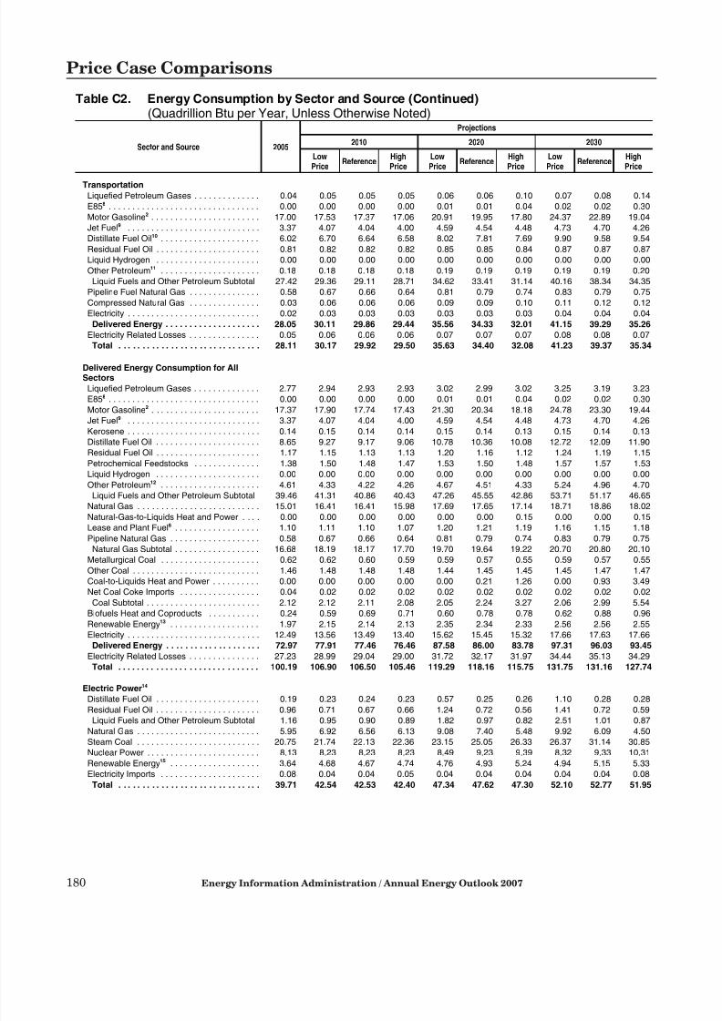
7/28/2019 2007 Annual Energy Outlook
http://slidepdf.com/reader/full/2007-annual-energy-outlook 189/243
180 Energy Information Administration / Annual Energy Outlook 2007
Price Case Comparisons
Table C2. Energy Consumption by Sector and Source (Continued)(Quadrillion Btu per Year, Unless Otherwise Noted)
Sector and Source 2005
Projections
2010 2020 2030
LowPrice
ReferenceHighPrice
LowPrice
ReferenceHighPrice
LowPrice
ReferenceHighPrice
Transportation
Liquefied Petroleum Gases . . . . . . . . . . . . . . 0.04 0.05 0.05 0.05 0.06 0.06 0.10 0.07 0.08 0.14
E858 . . . . . . . . . . . . . . . . . . . . . . . . . . . . . . . . 0.00 0.00 0.00 0.00 0.01 0.01 0.04 0.02 0.02 0.30
Motor Gasoline2 . . . . . . . . . . . . . . . . . . . . . . . 17.00 17.53 17.37 17.06 20.91 19.95 17.80 24.37 22.89 19.04
Jet Fuel9 . . . . . . . . . . . . . . . . . . . . . . . . . . . . 3.37 4.07 4.04 4.00 4.59 4.54 4.48 4.73 4.70 4.26
Distillate Fuel Oil10 . . . . . . . . . . . . . . . . . . . . . 6.02 6.70 6.64 6.58 8.02 7.81 7.69 9.90 9.58 9.54
Residual Fuel Oil . . . . . . . . . . . . . . . . . . . . . . 0.81 0.82 0.82 0.82 0.85 0.85 0.84 0.87 0.87 0.87
Liquid Hydrogen . . . . . . . . . . . . . . . . . . . . . . 0.00 0.00 0.00 0.00 0.00 0.00 0.00 0.00 0.00 0.00
Other Petroleum11 . . . . . . . . . . . . . . . . . . . . . 0.18 0.18 0.18 0.18 0.19 0.19 0.19 0.19 0.19 0.20
Liquid Fuels and Other Petroleum Subtotal 27.42 29.36 29.11 28.71 34.62 33.41 31.14 40.16 38.34 34.35
Pipeline Fuel Natural Gas . . . . . . . . . . . . . . . 0.58 0.67 0.66 0.64 0.81 0.79 0.74 0.83 0.79 0.75
Compressed Natural Gas . . . . . . . . . . . . . . . 0.03 0.06 0.06 0.06 0.09 0.09 0.10 0.11 0.12 0.12
Electricity . . . . . . . . . . . . . . . . . . . . . . . . . . . . 0.02 0.03 0.03 0.03 0.03 0.03 0.03 0.04 0.04 0.04
Delivered Energy . . . . . . . . . . . . . . . . . . . . 28.05 30.11 29.86 29.44 35.56 34.33 32.01 41.15 39.29 35.26
Electricity Related Losses . . . . . . . . . . . . . . . 0.05 0.06 0.06 0.06 0.07 0.07 0.07 0.08 0.08 0.07
Total . . . . . . . . . . . . . . . . . . . . . . . . . . . . . . 28.11 30.17 29.92 29.50 35.63 34.40 32.08 41.23 39.37 35.34
Delivered Energy Consumption for AllSectors
Liquefied Petroleum Gases . . . . . . . . . . . . . . 2.77 2.94 2.93 2.93 3.02 2.99 3.02 3.25 3.19 3.23
E858 . . . . . . . . . . . . . . . . . . . . . . . . . . . . . . . . 0.00 0.00 0.00 0.00 0.01 0.01 0.04 0.02 0.02 0.30
Motor Gasoline2 . . . . . . . . . . . . . . . . . . . . . . . 17.37 17.90 17.74 17.43 21.30 20.34 18.18 24.78 23.30 19.44
Jet Fuel9 . . . . . . . . . . . . . . . . . . . . . . . . . . . . 3.37 4.07 4.04 4.00 4.59 4.54 4.48 4.73 4.70 4.26
Kerosene . . . . . . . . . . . . . . . . . . . . . . . . . . . . 0.14 0.15 0.14 0.14 0.15 0.14 0.13 0.15 0.14 0.13
Distillate Fuel Oil . . . . . . . . . . . . . . . . . . . . . . 8.65 9.27 9.17 9.06 10.78 10.36 10.08 12.72 12.09 11.90
Residual Fuel Oil . . . . . . . . . . . . . . . . . . . . . . 1.17 1.15 1.13 1.13 1.20 1.16 1.12 1.24 1.19 1.15
Petrochemical Feedstocks . . . . . . . . . . . . . . 1.38 1.50 1.48 1.47 1.53 1.50 1.48 1.57 1.57 1.53
Liquid Hydrogen . . . . . . . . . . . . . . . . . . . . . . 0.00 0.00 0.00 0.00 0.00 0.00 0.00 0.00 0.00 0.00
Other Petroleum12 . . . . . . . . . . . . . . . . . . . . . 4.61 4.33 4.22 4.26 4.67 4.51 4.33 5.24 4.96 4.70
Liquid Fuels and Other Petroleum Subtotal 39.46 41.31 40.86 40.43 47.26 45.55 42.86 53.71 51.17 46.65
Natural Gas . . . . . . . . . . . . . . . . . . . . . . . . . . 15.01 16.41 16.41 15.98 17.69 17.65 17.14 18.71 18.86 18.02
Natural-Gas-to-Liquids Heat and Power . . . . 0.00 0.00 0.00 0.00 0.00 0.00 0.15 0.00 0.00 0.15
Lease and Plant Fuel6 . . . . . . . . . . . . . . . . . . 1.10 1.11 1.10 1.07 1.20 1.21 1.19 1.16 1.15 1.18
Pipeline Natural Gas . . . . . . . . . . . . . . . . . . . 0.58 0.67 0.66 0.64 0.81 0.79 0.74 0.83 0.79 0.75Natural Gas Subtotal . . . . . . . . . . . . . . . . . . 16.68 18.19 18.17 17.70 19.70 19.64 19.22 20.70 20.80 20.10
Metallurgical Coal . . . . . . . . . . . . . . . . . . . . . 0.62 0.62 0.60 0.59 0.59 0.57 0.55 0.59 0.57 0.55
Other Coal . . . . . . . . . . . . . . . . . . . . . . . . . . . 1.46 1.48 1.48 1.48 1.44 1.45 1.45 1.45 1.47 1.47
Coal-to-Liquids Heat and Power . . . . . . . . . . 0.00 0.00 0.00 0.00 0.00 0.21 1.26 0.00 0.93 3.49
Net Coal Coke Imports . . . . . . . . . . . . . . . . . 0.04 0.02 0.02 0.02 0.02 0.02 0.02 0.02 0.02 0.02
Coal Subtotal . . . . . . . . . . . . . . . . . . . . . . . . 2.12 2.12 2.11 2.08 2.05 2.24 3.27 2.06 2.99 5.54
Biofuels Heat and Coproducts . . . . . . . . . . . 0.24 0.59 0.69 0.71 0.60 0.78 0.78 0.62 0.88 0.96
Renewable Energy13 . . . . . . . . . . . . . . . . . . . 1.97 2.15 2.14 2.13 2.35 2.34 2.33 2.56 2.56 2.55
Electricity . . . . . . . . . . . . . . . . . . . . . . . . . . . . 12.49 13.56 13.49 13.40 15.62 15.45 15.32 17.66 17.63 17.66
Delivered Energy . . . . . . . . . . . . . . . . . . . . 72.97 77.91 77.46 76.46 87.58 86.00 83.78 97.31 96.03 93.45
Electricity Related Losses . . . . . . . . . . . . . . . 27.23 28.99 29.04 29.00 31.72 32.17 31.97 34.44 35.13 34.29
Total . . . . . . . . . . . . . . . . . . . . . . . . . . . . . . 100.19 106.90 106.50 105.46 119.29 118.16 115.75 131.75 131.16 127.74
Electric Power14
Distillate Fuel Oil . . . . . . . . . . . . . . . . . . . . . . 0.19 0.23 0.24 0.23 0.57 0.25 0.26 1.10 0.28 0.28
Residual Fuel Oil . . . . . . . . . . . . . . . . . . . . . . 0.96 0.71 0.67 0.66 1.24 0.72 0.56 1.41 0.72 0.59
Liquid Fuels and Other Petroleum Subtotal 1.16 0.95 0.90 0.89 1.82 0.97 0.82 2.51 1.01 0.87
Natural Gas . . . . . . . . . . . . . . . . . . . . . . . . . . 5.95 6.92 6.56 6.13 9.08 7.40 5.48 9.92 6.09 4.50
Steam Coal . . . . . . . . . . . . . . . . . . . . . . . . . . 20.75 21.74 22.13 22.36 23.15 25.05 26.33 26.37 31.14 30.85
Nuclear Power . . . . . . . . . . . . . . . . . . . . . . . . 8.13 8.23 8.23 8.23 8.49 9.23 9.39 8.32 9.33 10.31
Renewable Energy15 . . . . . . . . . . . . . . . . . . . 3.64 4.68 4.67 4.74 4.76 4.93 5.24 4.94 5.15 5.33
Electricity Imports . . . . . . . . . . . . . . . . . . . . . 0.08 0.04 0.04 0.05 0.04 0.04 0.04 0.04 0.04 0.08
Total . . . . . . . . . . . . . . . . . . . . . . . . . . . . . . 39.71 42.54 42.53 42.40 47.34 47.62 47.30 52.10 52.77 51.95

7/28/2019 2007 Annual Energy Outlook
http://slidepdf.com/reader/full/2007-annual-energy-outlook 190/243
Energy Information Administration / Annual Energy Outlook 2007 181
Price Case Comparisons
Table C2. Energy Consumption by Sector and Source (Continued)(Quadrillion Btu per Year, Unless Otherwise Noted)
Sector and Source 2005
Projections
2010 2020 2030
LowPrice
ReferenceHighPrice
LowPrice
ReferenceHighPrice
LowPrice
ReferenceHighPrice
Total Energy Consumption
Liquefied Petroleum Gases . . . . . . . . . . . . . . 2.77 2.94 2.93 2.93 3.02 2.99 3.02 3.25 3.19 3.23
E858 . . . . . . . . . . . . . . . . . . . . . . . . . . . . . . . . 0.00 0.00 0.00 0.00 0.01 0.01 0.04 0.02 0.02 0.30
Motor Gasoline2 . . . . . . . . . . . . . . . . . . . . . . . 17.37 17.90 17.74 17.43 21.30 20.34 18.18 24.78 23.30 19.44
Jet Fuel9 . . . . . . . . . . . . . . . . . . . . . . . . . . . . 3.37 4.07 4.04 4.00 4.59 4.54 4.48 4.73 4.70 4.26
Kerosene . . . . . . . . . . . . . . . . . . . . . . . . . . . . 0.14 0.15 0.14 0.14 0.15 0.14 0.13 0.15 0.14 0.13
Distillate Fuel Oil . . . . . . . . . . . . . . . . . . . . . . 8.84 9.51 9.40 9.30 11.36 10.61 10.34 13.82 12.37 12.17
Residual Fuel Oil . . . . . . . . . . . . . . . . . . . . . . 2.14 1.86 1.80 1.79 2.44 1.88 1.68 2.65 1.91 1.74
Petrochemical Feedstocks . . . . . . . . . . . . . . 1.38 1.50 1.48 1.47 1.53 1.50 1.48 1.57 1.57 1.53
Liquid Hydrogen . . . . . . . . . . . . . . . . . . . . . . 0.00 0.00 0.00 0.00 0.00 0.00 0.00 0.00 0.00 0.00
Other Petroleum12 . . . . . . . . . . . . . . . . . . . . . 4.61 4.33 4.22 4.26 4.67 4.51 4.33 5.24 4.96 4.70
Liquid Fuels and Other Petroleum Subtotal 40.61 42.25 41.76 41.32 49.08 46.52 43.68 56.22 52.17 47.52
Natural Gas . . . . . . . . . . . . . . . . . . . . . . . . . . 20.96 23.33 22.97 22.12 26.77 25.05 22.62 28.63 24.95 22.52
Natural-Gas-to-Liquids Heat and Power . . . . 0.00 0.00 0.00 0.00 0.00 0.00 0.15 0.00 0.00 0.15
Lease and Plant Fuel6 . . . . . . . . . . . . . . . . . . 1.10 1.11 1.10 1.07 1.20 1.21 1.19 1.16 1.15 1.18
Pipeline Natural Gas . . . . . . . . . . . . . . . . . . . 0.58 0.67 0.66 0.64 0.81 0.79 0.74 0.83 0.79 0.75
Natural Gas Subtotal . . . . . . . . . . . . . . . . . . 22.63 25.11 24.73 23.83 28.78 27.04 24.70 30.62 26.89 24.60Metallurgical Coal . . . . . . . . . . . . . . . . . . . . . 0.62 0.62 0.60 0.59 0.59 0.57 0.55 0.59 0.57 0.55
Other Coal . . . . . . . . . . . . . . . . . . . . . . . . . . . 22.21 23.22 23.61 23.84 24.59 26.50 27.78 27.82 32.61 32.32
Coal-to-Liquids Heat and Power . . . . . . . . . . 0.00 0.00 0.00 0.00 0.00 0.21 1.26 0.00 0.93 3.49
Net Coal Coke Imports . . . . . . . . . . . . . . . . . 0.04 0.02 0.02 0.02 0.02 0.02 0.02 0.02 0.02 0.02
Coal Subtotal . . . . . . . . . . . . . . . . . . . . . . . . 22.87 23.86 24.24 24.45 25.20 27.29 29.60 28.43 34.14 36.39
Nuclear Power . . . . . . . . . . . . . . . . . . . . . . . . 8.13 8.23 8.23 8.23 8.49 9.23 9.39 8.32 9.33 10.31
Biofuels Heat and Coproducts . . . . . . . . . . . 0.24 0.59 0.69 0.71 0.60 0.78 0.78 0.62 0.88 0.96
Renewable Energy16 . . . . . . . . . . . . . . . . . . . 5.61 6.83 6.81 6.87 7.10 7.27 7.57 7.50 7.71 7.89
Electricity Imports . . . . . . . . . . . . . . . . . . . . . 0.08 0.04 0.04 0.05 0.04 0.04 0.04 0.04 0.04 0.08
Total . . . . . . . . . . . . . . . . . . . . . . . . . . . . . . 100.19 106.90 106.50 105.46 119.29 118.16 115.75 131.75 131.16 127.74
Energy Use and Related Statistics
Delivered Energy Use . . . . . . . . . . . . . . . . . . . 72.97 77.91 77.46 76.46 87.58 86.00 83.78 97.31 96.03 93.45
Total Energy Use . . . . . . . . . . . . . . . . . . . . . . . 100.19 106.90 106.50 105.46 119.29 118.16 115.75 131.75 131.16 127.74
Ethanol Consumed in Motor Gasoline and E85 0.33 0.77 0.91 0.95 0.79 1.06 1.05 0.87 1.22 1.30
Population (millions) . . . . . . . . . . . . . . . . . . . . . 296.94 310.26 310.26 310.26 337.13 337.13 337.13 364.94 364.94 364.94Gross Domestic Product (billion 2000 dollars) . 11049 12850 12790 12708 17129 17077 17027 22532 22494 22472
Carbon Dioxide Emissions (million metric tons) 5945.3 6241.2 6214.0 6155.6 7040.2 6944.5 6830.5 7928.6 7950.2 7701.0
1Includes wood used for residential heating. See Table A4 and/or Table A17 for estimates of nonmarketed renewable energy consumption for geothermal heat pumps, solarthermal hot water heating, and solar photovoltaic electricity generation.
2Includes ethanol (blends of 10 percent or less) and ethers blended into gasoline.3Includes commercial sector consumption of wood and wood waste, landfill gas, municipal solid waste, and other biomass for combined heat and power. See Table A5
and/or Table A17 for estimates of nonmarketed renewable energy consumption for solar thermal hot water heating and solar photovoltaic electricity generation.4Includes energy for combined heat and power plants, except those whose primary business is to sell electricity, or electricity and heat, to the public.5Includes petroleum coke, asphalt, road oil, lubricants, still gas, tire-derived fuel, and miscellaneous petroleum products.6Represents natural gas used in well, field, and lease operations, and in natural gas processing plant machinery.7Includes consumption of energy produced from hydroelectric, wood and wood waste, municipal solid waste, and other biomass sources.8E85 refers to a blend of 85 percent ethanol (renewable) and 15 percent motor gasoline (nonrenewable). To address cold starting issues, the percentage of ethanol actually
varies seasonally. The annual average ethanol content of 74 percent is used for this forecast.9Includes only kerosene type.10Diesel fuel for on- and off- road use.11Includes aviation gasoline and lubricants.12Includes unfinished oils, natural gasoline, motor gasoline blending components, aviation gasoline, lubricants, still gas, asphalt, road oil, petroleum coke, tire-derived fuel,
and miscellaneous petroleum products.13Includes electricity generated for sale to the grid and for own use from renewable sources, and non-electric energy from renewable sources. Excludes nonmarketed
renewable energy consumption for geothermal heat pumps, buildings photovoltaic systems, and solar thermal hot water heaters.14Includes consumption of energy by electricity-only and combined heat and power plants whose primary business is to sell electricity, or electricity and heat, to the public.
Includes small power producers and exempt wholesale generators.15Includes conventional hydroelectric, geothermal, wood and wood waste, municipal solid waste, other biomass, petroleum coke, wind, photovoltaic and solar thermal
sources. Excludes net electricity imports.16Includes hydroelectric, geothermal, wood and wood waste, municipal solid waste, other biomass, wind, photovoltaic and solar thermal sources. Includes ethanol
components of E85; excludes ethanol blends (10 percent or less) in motor gasoline. Excludes net electricity imports and nonmarketed renewable energy consumption forgeothermal heat pumps, buildings photovoltaic systems, and solar thermal hot water heaters.
Btu = British thermal unit.N/A = Not applicable.Note: Totals may not equal sum of components due to independent rounding. Data for 2005 are model results and may differ slightly from official EIA data reports.
Consumption values of 0.00 are values that round to 0.00, because they are less than 0.005.Sources: 2005 consumption based on: Energy Information Administration (EIA), Annual Energy Review 2005 , DOE/EIA-0384(2005) (Washington, DC, July 2006). 2005
population and gross domestic product: Global Insight macroeconomic model CTL0806. 2005 carbon dioxide emissions: EIA, Emissions of Greenhouse Gases in the United States 2005, DOE/EIA-0573(2005) (Washington, DC, November 2006). Projections: EIA, AEO2007 National Energy Modeling System runs LP2007.D112106A,AEO2007.D112106A, and HP2007.D112106A.

7/28/2019 2007 Annual Energy Outlook
http://slidepdf.com/reader/full/2007-annual-energy-outlook 191/243
182 Energy Information Administration / Annual Energy Outlook 2007
Price Case Comparisons
Table C3. Energy Prices by Sector and Source(2005 Dollars per Million Btu, Unless Otherwise Noted)
Sector and Source 2005
Projections
2010 2020 2030
LowPrice
ReferenceHighPrice
LowPrice
ReferenceHighPrice
LowPrice
ReferenceHighPrice
Residential
Liquefied Petroleum Gases . . . . . . . . . . . . . . . 19.29 23.03 23.67 24.29 22.18 23.18 23.92 22.98 23.91 25.65
Distillate Fuel Oil . . . . . . . . . . . . . . . . . . . . . . . 14.73 12.63 14.87 16.58 9.09 13.15 18.95 9.66 14.13 19.84
Natural Gas . . . . . . . . . . . . . . . . . . . . . . . . . . . 12.43 10.33 10.98 11.59 9.50 10.54 11.29 10.40 11.43 13.12
Electricity . . . . . . . . . . . . . . . . . . . . . . . . . . . . . 27.59 26.24 26.91 27.58 25.24 26.37 26.96 26.08 26.76 27.24
Commercial
Distillate Fuel Oil . . . . . . . . . . . . . . . . . . . . . . . 12.68 10.58 12.72 14.58 7.15 11.35 16.85 7.88 12.45 18.06
Residual Fuel Oil . . . . . . . . . . . . . . . . . . . . . . . 8.41 6.61 7.54 7.31 4.39 7.07 11.35 4.59 7.31 12.07
Natural Gas . . . . . . . . . . . . . . . . . . . . . . . . . . . 11.20 8.70 9.34 9.94 7.65 8.67 9.41 8.33 9.30 10.99
Electricity . . . . . . . . . . . . . . . . . . . . . . . . . . . . . 25.25 23.69 24.50 25.28 22.58 23.95 24.67 23.39 24.27 25.26
Industrial1
Liquefied Petroleum Gases . . . . . . . . . . . . . . . 16.96 15.79 16.42 17.09 14.89 15.91 16.66 15.75 16.55 18.25
Distillate Fuel Oil . . . . . . . . . . . . . . . . . . . . . . . 13.08 10.93 12.95 14.94 7.90 12.04 17.30 8.84 13.25 18.79
Residual Fuel Oil . . . . . . . . . . . . . . . . . . . . . . . 7.77 8.42 9.50 10.74 6.15 8.91 14.15 6.41 9.58 15.36
Natural Gas2
. . . . . . . . . . . . . . . . . . . . . . . . . . 8.16 5.83 6.43 7.03 4.92 5.90 6.61 5.65 6.56 8.21Metallurgical Coal . . . . . . . . . . . . . . . . . . . . . . 3.06 3.08 3.09 3.11 2.69 2.71 2.76 2.73 2.75 2.78
Other Industrial Coal . . . . . . . . . . . . . . . . . . . . 2.15 2.22 2.26 2.30 2.07 2.18 2.32 2.12 2.29 2.43
Coal to Liquids . . . . . . . . . . . . . . . . . . . . . . . . . 0.00 0.00 0.00 0.00 0.00 0.97 1.42 0.00 1.33 1.78
Electricity . . . . . . . . . . . . . . . . . . . . . . . . . . . . . 16.69 17.35 18.01 18.64 16.11 17.07 17.41 16.95 17.43 17.72
Transportation
Liquefied Petroleum Gases3 . . . . . . . . . . . . . . 23.92 23.72 24.34 24.88 22.68 23.66 24.20 23.35 24.29 25.85
E854 . . . . . . . . . . . . . . . . . . . . . . . . . . . . . . . . . 23.10 22.00 21.29 22.41 18.58 20.61 23.33 19.38 21.50 25.54
Motor Gasoline5 . . . . . . . . . . . . . . . . . . . . . . . . 18.64 16.55 17.90 20.64 13.97 16.63 23.62 14.39 17.76 26.42
Jet Fuel6 . . . . . . . . . . . . . . . . . . . . . . . . . . . . . 13.14 9.66 10.91 12.84 7.43 10.51 15.86 8.21 11.75 17.44
Distillate Fuel Oil7 . . . . . . . . . . . . . . . . . . . . . . 17.52 14.79 16.81 18.76 11.24 15.42 20.72 12.02 16.47 22.20
Residual Fuel Oil . . . . . . . . . . . . . . . . . . . . . . . 5.51 6.89 8.05 9.83 4.76 7.36 12.85 5.03 8.27 14.38
Natural Gas8 . . . . . . . . . . . . . . . . . . . . . . . . . . 14.76 13.27 13.97 14.90 11.66 12.98 14.98 11.99 13.45 16.55
Electricity . . . . . . . . . . . . . . . . . . . . . . . . . . . . . 25.22 23.98 24.86 25.66 22.90 24.22 24.77 23.72 24.46 25.19
Electric Power9
Distillate Fuel Oil . . . . . . . . . . . . . . . . . . . . . . . 11.38 9.44 11.71 13.59 5.07 9.84 15.34 5.43 10.79 15.94Residual Fuel Oil . . . . . . . . . . . . . . . . . . . . . . . 6.96 5.64 6.58 7.59 3.51 6.08 11.24 3.68 6.85 12.57
Natural Gas . . . . . . . . . . . . . . . . . . . . . . . . . . . 8.18 5.64 6.22 6.75 4.93 5.76 6.32 5.71 6.33 7.79
Steam Coal . . . . . . . . . . . . . . . . . . . . . . . . . . . 1.53 1.67 1.71 1.74 1.48 1.58 1.71 1.51 1.69 1.80
Average Price to All Users10
Liquefied Petroleum Gases . . . . . . . . . . . . . . . 17.48 17.39 18.02 18.68 16.60 17.62 18.44 17.44 18.30 20.13
E854 . . . . . . . . . . . . . . . . . . . . . . . . . . . . . . . . . 23.10 22.00 21.29 22.41 18.58 20.61 23.33 19.38 21.50 25.54
Motor Gasoline5 . . . . . . . . . . . . . . . . . . . . . . . . 18.60 16.55 17.90 20.64 13.97 16.63 23.61 14.39 17.75 26.42
Jet Fuel . . . . . . . . . . . . . . . . . . . . . . . . . . . . . . 13.14 9.66 10.91 12.84 7.43 10.51 15.86 8.21 11.75 17.44
Distillate Fuel Oil . . . . . . . . . . . . . . . . . . . . . . . 16.22 13.66 15.70 17.64 10.18 14.53 19.89 10.85 15.70 21.45
Residual Fuel Oil . . . . . . . . . . . . . . . . . . . . . . . 6.59 6.54 7.61 8.90 4.22 7.00 12.31 4.39 7.79 13.68
Natural Gas . . . . . . . . . . . . . . . . . . . . . . . . . . . 9.65 7.22 7.83 8.46 6.30 7.32 8.15 7.04 8.09 9.85
Metallurgical Coal . . . . . . . . . . . . . . . . . . . . . . 3.06 3.08 3.09 3.11 2.69 2.71 2.76 2.73 2.75 2.78
Other Coal . . . . . . . . . . . . . . . . . . . . . . . . . . . . 1.57 1.70 1.74 1.77 1.52 1.61 1.74 1.54 1.72 1.83
Coal to Liquids . . . . . . . . . . . . . . . . . . . . . . . . . 0.00 0.00 0.00 0.00 0.00 0.97 1.42 0.00 1.33 1.78
Electricity . . . . . . . . . . . . . . . . . . . . . . . . . . . . . 23.73 22.94 23.66 24.37 21.98 23.15 23.73 22.92 23.60 24.18

7/28/2019 2007 Annual Energy Outlook
http://slidepdf.com/reader/full/2007-annual-energy-outlook 192/243
Energy Information Administration / Annual Energy Outlook 2007 183
Price Case Comparisons
Table C3. Energy Prices by Sector and Source (Continued)(2005 Dollars per Million Btu, Unless Otherwise Noted)
Sector and Source 2005
Projections
2010 2020 2030
LowPrice
ReferenceHighPrice
LowPrice
ReferenceHighPrice
LowPrice
ReferenceHighPrice
Non-Renewable Energy Expenditures by
Sector (billion 2005 dollars)
Residential . . . . . . . . . . . . . . . . . . . . . . . . . . . . 215.13 212.43 220.44 227.60 222.50 236.03 246.06 250.70 262.21 276.15
Commercial . . . . . . . . . . . . . . . . . . . . . . . . . . . 154.38 151.98 157.97 163.50 170.74 181.74 188.76 212.65 222.08 234.83
Industrial . . . . . . . . . . . . . . . . . . . . . . . . . . . . . 196.07 187.02 200.48 213.85 169.84 194.88 224.73 193.83 222.08 269.71
Transportation . . . . . . . . . . . . . . . . . . . . . . . . . 474.66 437.09 476.38 538.62 424.57 511.07 668.16 517.92 632.79 811.45
Total Non-Renewable Expenditures . . . . . . . 1040.25 988.51 1055.27 1143.57 987.65 1123.73 1327.72 1175.11 1339.16 1592.14
Transportation Renewable Expenditures . . . 0.03 0.05 0.06 0.09 0.13 0.15 0.89 0.40 0.51 7.62
Total Expenditures . . . . . . . . . . . . . . . . . . . 1040.29 988.56 1055.33 1143.66 987.78 1123.89 1328.60 1175.51 1339.68 1599.77
1Includes energy for combined heat and power plants, except those whose primary business is to sell electricity, or electricity and heat, to the public.2Excludes use for lease and plant fuel.3Includes Federal and State taxes while excluding county and local taxes.4E85 refers to a blend of 85 percent ethanol (renewable) and 15 percent motor gasoline (nonrenewable). To address cold starting issues, the percentage of ethanol actually
varies seasonally. The annual average ethanol content of 74 percent is used for this forecast.5Sales weighted-average price for all grades. Includes Federal, State and local taxes.6Kerosene-type jet fuel. Includes Federal and State taxes while excluding county and local taxes.7Diesel fuel for on-road use. Includes Federal and State taxes while excluding county and local taxes.8Compressed natural gas used as a vehicle fuel. Includes estimated motor vehicle fuel taxes and estimated dispensing costs or charges.9Includes electricity-only and combined heat and power plants whose primary business is to sell electricity, or electricity and heat, to the public.10Weighted averages of end-use fuel prices are derived from the prices shown in each sector and the corresponding sectoral consumption.Btu = British thermal unit.N/A = Not applicable.Note: Data for 2005 are model results and may differ slightly from official EIA data reports.Sources: 2005 prices for motor gasoline, distillate fuel oil, and jet fuel are based on prices in the Energy Information Administration (EIA), Petroleum Marketing Annual
2005 , DOE/EIA-0487(2005) (Washington, DC, August 2006). 2005 residential and commercial natural gas delivered prices: EIA, Natural Gas Monthly , DOE/EIA-0130(2006/04) (Washington, DC, April 2006). 2005 industrial natural gas delivered prices are estimated based on: EIA, Manufacturing Energy Consumption Survey 1994 andindustrial and wellhead prices from the Natural Gas Annual 2004 , DOE/EIA-0131(2004) (Washington, DC, December 2005) and the Natural Gas Monthly , DOE/EIA-0130(2006/04) (Washington, DC, April 2006). 2005 transportation sector natural gas delivered prices are model results. 2005 electric power sector natural gas prices: EIA,Electric Power Monthly , DOE/EIA-0226, May 2003 through April 2004, Table 4.11.A. 2005 coal prices based on: EIA, Quarterly Coal Report, October-December 2005 ,DOE/EIA-0121(2005/4Q) (Washington, DC, March 2006) and EIA, AEO2007 National Energy Modeling System run AEO2007.D112106A. 2005 electricity prices: EIA, Annual Energy Review 2005 , DOE/EIA-0384(2005) (Washington, DC, July 2006). 2005 ethanol prices derived from weekly spot prices in the Oxy Fuel News. Projections: EIA,AEO2007 National Energy Modeling System runs LP2007.D112106A, AEO2007.D112106A, and HP2007.D112106A.

7/28/2019 2007 Annual Energy Outlook
http://slidepdf.com/reader/full/2007-annual-energy-outlook 193/243
184 Energy Information Administration / Annual Energy Outlook 2007
Price Case Comparisons
Table C4. Liquid Fuels Supply and Disposition(Million Barrels per Day, Unless Otherwise Noted)
Supply and Disposition 2005
Projections
2010 2020 2030
LowPrice
ReferenceHighPrice
LowPrice
ReferenceHighPrice
LowPrice
ReferenceHighPrice
Crude Oil
Domestic Crude Production1 . . . . . . . . . . . . . . 5.18 5.81 5.67 5.51 5.95 5.89 5.98 5.25 5.39 6.04
Alaska . . . . . . . . . . . . . . . . . . . . . . . . . . . . . . 0.86 0.69 0.69 0.69 0.69 0.74 0.71 0.25 0.27 0.42
Lower 48 States . . . . . . . . . . . . . . . . . . . . . . 4.31 5.12 4.98 4.82 5.25 5.15 5.28 4.99 5.12 5.62
Net Imports . . . . . . . . . . . . . . . . . . . . . . . . . . . 10.09 9.94 9.99 10.01 11.69 11.29 10.02 14.35 13.09 10.59
Gross Imports . . . . . . . . . . . . . . . . . . . . . . . . 10.12 9.98 10.03 10.05 11.73 11.33 10.06 14.38 13.12 10.63
Exports . . . . . . . . . . . . . . . . . . . . . . . . . . . . . 0.03 0.04 0.04 0.03 0.04 0.04 0.04 0.03 0.03 0.04
Other Crude Supply2 . . . . . . . . . . . . . . . . . . . . -0.06 0.00 0.00 0.00 0.00 0.00 0.00 0.00 0.00 0.00
Total Crude Supply . . . . . . . . . . . . . . . . . . 15.22 15.75 15.66 15.52 17.64 17.19 16.00 19.60 18.47 16.63
Other Supply
Natural Gas Plant Liquids . . . . . . . . . . . . . . . . 1.72 1.82 1.80 1.76 1.77 1.76 1.69 1.73 1.72 1.71
Net Product Imports . . . . . . . . . . . . . . . . . . . . 2.48 1.99 1.80 1.72 3.46 2.27 1.53 4.95 3.28 1.45
Gross Refined Product Imports3 . . . . . . . . . . 2.45 1.99 1.78 1.76 2.83 1.98 1.52 3.73 2.52 1.43
Unfinished Oil Imports . . . . . . . . . . . . . . . . . 0.58 0.42 0.41 0.36 0.66 0.51 0.42 0.90 0.67 0.43
Ethanol Imports . . . . . . . . . . . . . . . . . . . . . . 0.01 0.01 0.02 0.02 0.01 0.04 0.04 0.05 0.05 0.05
Blending Component Imports . . . . . . . . . . . . 0.54 0.82 0.82 0.80 1.29 1.03 0.79 1.72 1.36 0.81Exports . . . . . . . . . . . . . . . . . . . . . . . . . . . . . 1.07 1.25 1.23 1.22 1.33 1.29 1.25 1.44 1.33 1.28
Refinery Processing Gain4 . . . . . . . . . . . . . . . 0.99 1.18 1.21 1.16 1.18 1.41 1.28 1.22 1.49 1.37
Other Inputs . . . . . . . . . . . . . . . . . . . . . . . . . . . 0.39 0.96 1.02 1.13 1.07 1.31 1.98 1.19 1.88 3.30
Ethanol . . . . . . . . . . . . . . . . . . . . . . . . . . . . . 0.26 0.59 0.69 0.72 0.60 0.79 0.78 0.63 0.90 0.96
Liquids from Gas . . . . . . . . . . . . . . . . . . . . . 0.00 0.00 0.00 0.00 0.00 0.00 0.10 0.00 0.00 0.10
Liquids from Coal . . . . . . . . . . . . . . . . . . . . . 0.00 0.00 0.00 0.00 0.00 0.10 0.60 0.00 0.44 1.65
Other5 . . . . . . . . . . . . . . . . . . . . . . . . . . . . . . 0.13 0.36 0.33 0.41 0.47 0.43 0.50 0.57 0.53 0.59
Total Primary Supply6 . . . . . . . . . . . . . . . . . . . 20.79 21.70 21.49 21.28 25.13 23.94 22.48 28.70 26.84 24.46
Liquid Fuels Consumption
by Fuel
Liquefied Petroleum Gases . . . . . . . . . . . . . 2.03 2.22 2.22 2.21 2.28 2.26 2.29 2.46 2.42 2.45
E857 . . . . . . . . . . . . . . . . . . . . . . . . . . . . . . . 0.00 0.00 0.00 0.00 0.01 0.01 0.03 0.01 0.02 0.21
Motor Gasoline8 . . . . . . . . . . . . . . . . . . . . . . 9.16 9.58 9.53 9.38 11.37 10.93 9.79 13.23 12.53 10.47
Jet Fuel9 . . . . . . . . . . . . . . . . . . . . . . . . . . . . 1.68 1.97 1.95 1.94 2.22 2.19 2.16 2.29 2.27 2.06
Distillate Fuel Oil10 . . . . . . . . . . . . . . . . . . . . 4.12 4.58 4.53 4.48 5.47 5.11 4.98 6.64 5.95 5.85Residual Fuel Oil . . . . . . . . . . . . . . . . . . . . . 0.92 0.81 0.79 0.78 1.06 0.82 0.73 1.16 0.83 0.76
Other11 . . . . . . . . . . . . . . . . . . . . . . . . . . . . . 2.84 2.63 2.57 2.58 2.79 2.70 2.61 3.06 2.93 2.80
by Sector
Residential and Commercial . . . . . . . . . . . . 1.26 1.28 1.25 1.24 1.39 1.29 1.21 1.41 1.28 1.19
Industrial12 . . . . . . . . . . . . . . . . . . . . . . . . . . 5.07 5.08 5.01 5.00 5.30 5.16 5.04 5.75 5.53 5.37
Transportation . . . . . . . . . . . . . . . . . . . . . . . 13.87 15.01 14.93 14.74 17.71 17.15 15.97 20.55 19.69 17.64
Electric Power13 . . . . . . . . . . . . . . . . . . . . . . 0.51 0.42 0.40 0.40 0.81 0.43 0.37 1.13 0.45 0.39
Total . . . . . . . . . . . . . . . . . . . . . . . . . . . . . . . . 20.75 21.79 21.59 21.37 25.21 24.03 22.59 28.84 26.95 24.60
Discrepancy14 . . . . . . . . . . . . . . . . . . . . . . . . . . 0.04 -0.09 -0.10 -0.09 -0.08 -0.09 -0.11 -0.14 -0.11 -0.13

7/28/2019 2007 Annual Energy Outlook
http://slidepdf.com/reader/full/2007-annual-energy-outlook 194/243
Energy Information Administration / Annual Energy Outlook 2007 185
Price Case Comparisons
Table C4. Liquid Fuels Supply and Disposition (Continued)(Million Barrels per Day, Unless Otherwise Noted)
Supply and Disposition 2005
Projections
2010 2020 2030
LowPrice
ReferenceHighPrice
LowPrice
ReferenceHighPrice
LowPrice
ReferenceHighPrice
Domestic Refinery Distillation Capacity15 . . . . . . 17.1 17.9 17.8 18.0 19.0 18.7 18.1 21.0 20.0 18.5
Capacity Utilization Rate (percent)16 . . . . . . . . . 91.0 89.4 89.1 87.5 94.2 93.4 89.6 94.7 93.5 91.1
Net Import Share of Product Supplied (percent) 60.5 55.0 54.9 55.1 60.3 56.6 51.4 67.3 61.0 49.2
Net Expenditures for Imported Crude Oil and
Petroleum Products (billion 2005 dollars) . . . . 236.65 194.59 222.76 268.39 161.96 229.80 344.40 211.83 300.51 404.77
1Includes lease condensate.2Strategic petroleum reserve stock additions plus unaccounted for crude oil and crude stock withdrawals minus crude product supplied.3Includes other hydrocarbons and alcohols.4Represents volumetric gain in refinery distillation and cracking processes.5Includes petroleum product stock withdrawals, domestic sources of blending components, other hydrocarbons, ethers, and renewable fuels such as biodiesel.6Total crude supply plus natural gas plant liquids, other inputs, refinery processing gain, and net product imports.7E85 refers to a blend of 85 percent ethanol (renewable) and 15 percent motor gasoline (nonrenewable). To address cold starting issues, the percentage of ethanol actually
varies seasonally. The annual average ethanol content of 74 percent is used for this forecast.8Includes ethanol and ethers blended into gasoline.9Includes only kerosene type.10Includes distillate fuel oil and kerosene from petroleum and biomass feedstocks.11
Includes aviation gasoline, petrochemical feedstocks, lubricants, waxes, asphalt, road oil, still gas, special naphthas, petroleum coke, crude oil product supplied, tire-derived fuel, methanol, liquid hydrogen,and miscellaneous petroleum products.12Includes consumption for combined heat and power, which produces electricity and other useful thermal energy.13Includes consumption of energy by electricity-only and combined heat and power plants whose primary business is to sell electricity, or electricity and heat, to the public.
Includes small power producers and exempt wholesale generators.14Balancing item. Includes unaccounted for supply, losses, and gains.15End-of-year operable capacity.16Rate is calculated by dividing the gross annual input to atmospheric crude oil distillation units by their operable refining capacity in barrels per calendar day.N/A = Not applicable.Note: Totals may not equal sum of components due to independent rounding. Data for 2005 are model results and may differ slightly from official EIA data reports.Sources: 2005 imported crude oil price and petroleum product supplied based on: Energy Information Administration (EIA), Annual Energy Review 2005 , DOE/EIA-
0384(2005) (Washington, DC, July 2006). 2005 imported low sulfur light crude oil price: EIA, Form EIA-856, “Monthly Foreign Crude Oil Acquisition Report.” Other 2005 data:EIA, Petroleum Supply Annual 2005, DOE/EIA-0340(2005)/1 (Washington, DC, October 2006). Projections: EIA, AEO2007 National Energy Modeling System runsLP2007.D112106A, AEO2007.D112106A, and HP2007.D112106A.

7/28/2019 2007 Annual Energy Outlook
http://slidepdf.com/reader/full/2007-annual-energy-outlook 195/243
186 Energy Information Administration / Annual Energy Outlook 2007
Price Case Comparisons
Table C5. Petroleum Product Prices(2005 Cents per Gallon, Unless Otherwise Noted)
Sector and Fuel 2005
Projections
2010 2020 2030
LowPrice
ReferenceHighPrice
LowPrice
ReferenceHighPrice
LowPrice
ReferenceHighPrice
Crude Oil Prices (2005 dollars per barrel)
Imported Low Sulfur Light Crude Oil1 . . . . . . . 56.76 49.21 57.47 69.21 34.10 52.04 89.12 35.68 59.12 100.14
Imported Crude Oil1 . . . . . . . . . . . . . . . . . . . . . 49.19 44.06 51.20 62.53 28.91 46.47 82.60 28.91 51.63 92.93
Delivered Sector Product Prices
Residential
Liquefied Petroleum Gases . . . . . . . . . . . . . 166.3 198.5 204.0 209.4 191.1 199.8 206.2 198.0 206.1 221.0
Distillate Fuel Oil . . . . . . . . . . . . . . . . . . . . . 204.3 175.2 206.3 229.9 126.1 182.3 262.8 134.0 195.9 275.1
Commercial
Distillate Fuel Oil . . . . . . . . . . . . . . . . . . . . . 175.4 145.9 175.5 201.2 98.6 156.5 232.3 108.6 171.7 248.9
Residual Fuel Oil . . . . . . . . . . . . . . . . . . . . . 126.0 99.0 112.8 109.5 65.8 105.8 169.8 68.7 109.4 180.7
Residual Fuel Oil (2005 dollars per barrel) . 52.90 41.56 47.39 45.99 27.62 44.44 71.33 28.85 45.97 75.89
Industrial2
Liquefied Petroleum Gases . . . . . . . . . . . . . 146.2 136.1 141.5 147.3 128.3 137.1 143.6 135.7 142.6 157.3Distillate Fuel Oil . . . . . . . . . . . . . . . . . . . . . 181.1 150.3 178.1 205.4 108.5 165.3 237.5 121.4 181.8 257.9
Residual Fuel Oil . . . . . . . . . . . . . . . . . . . . . 116.3 126.0 142.2 160.8 92.1 133.4 211.9 95.9 143.5 230.0
Residual Fuel Oil (2005 dollars per barrel) . 48.86 52.94 59.74 67.52 38.68 56.04 88.98 40.29 60.25 96.58
Transportation
Liquefied Petroleum Gases . . . . . . . . . . . . . 206.1 204.4 209.8 214.4 195.5 203.9 208.6 201.2 209.3 222.8
Ethanol (E85)3 . . . . . . . . . . . . . . . . . . . . . . . 217.1 205.4 198.5 208.8 173.6 192.1 217.3 181.0 200.4 237.9
Ethanol Wholesale Price . . . . . . . . . . . . . . . 180.4 174.8 181.4 184.0 152.3 168.2 174.0 155.3 170.2 183.5
Motor Gasoline4 . . . . . . . . . . . . . . . . . . . . . . 231.6 201.8 217.3 250.1 170.7 201.9 286.1 175.8 215.4 320.1
Jet Fuel5 . . . . . . . . . . . . . . . . . . . . . . . . . . . . 177.4 130.5 147.2 173.3 100.3 141.8 214.1 110.8 158.6 235.5
Diesel Fuel (distillate fuel oil)6 . . . . . . . . . . . 241.3 202.7 230.4 257.2 154.1 211.2 283.9 164.7 225.7 304.2
Residual Fuel Oil . . . . . . . . . . . . . . . . . . . . . 82.4 103.2 120.5 147.2 71.2 110.2 192.4 75.2 123.8 215.2
Residual Fuel Oil (2005 dollars per barrel) . 34.62 43.33 50.60 61.81 29.91 46.27 80.79 31.60 52.02 90.40
Electric Power7
Distillate Fuel Oil . . . . . . . . . . . . . . . . . . . . . 157.9 130.9 162.3 188.5 70.3 136.5 212.7 75.4 149.6 221.1
Residual Fuel Oil . . . . . . . . . . . . . . . . . . . . . 104.2 84.4 98.5 113.7 52.6 91.0 168.3 55.0 102.5 188.1Residual Fuel Oil (2005 dollars per barrel) . 43.76 35.44 41.37 47.75 22.10 38.24 70.69 23.11 43.05 79.02
Refined Petroleum Product Prices8
Liquefied Petroleum Gases . . . . . . . . . . . . . 150.7 149.9 155.3 161.0 143.1 151.9 158.9 150.3 157.7 173.5
Motor Gasoline4 . . . . . . . . . . . . . . . . . . . . . . 231.1 201.8 217.3 250.1 170.6 201.8 286.0 175.8 215.4 320.1
Jet Fuel5 . . . . . . . . . . . . . . . . . . . . . . . . . . . . 177.4 130.5 147.2 173.3 100.3 141.8 214.1 110.8 158.6 235.5
Distillate Fuel Oil . . . . . . . . . . . . . . . . . . . . . 223.9 187.8 215.9 242.5 139.8 199.4 273.0 149.0 215.5 294.4
Residual Fuel Oil . . . . . . . . . . . . . . . . . . . . . 98.6 97.9 113.9 133.3 63.1 104.7 184.3 65.8 116.6 204.8
Residual Fuel Oil (2005 dollars per barrel) . 41.42 41.10 47.84 55.97 26.50 43.98 77.40 27.63 48.96 86.01
Average . . . . . . . . . . . . . . . . . . . . . . . . . . 204.5 177.5 195.0 221.3 145.8 183.4 253.3 153.5 198.1 281.4
1Weighted average price delivered to U.S. refiners.2Includes energy for combined heat and power plants, except those whose primary business is to sell electricity, or electricity and heat, to the public.3E85 refers to a blend of 85 percent ethanol (renewable) and 15 percent motor gasoline (nonrenewable). To address cold starting issues, the percentage of ethanol actually
varies seasonally. The annual average ethanol content of 74 percent is used for this forecast.4Sales weighted-average price for all grades. Includes Federal, State and local taxes.5Includes only kerosene type.6Diesel fuel for on-road use. Includes Federal and State taxes while excluding county and local taxes.7Includes electricity-only and combined heat and power plants whose primary business is to sell electricity, or electricity and heat, to the public. Includes small power
producers and exempt wholesale generators.8Weighted averages of end-use fuel prices are derived from the prices in each sector and the corresponding sectoral consumption.Note: Data for 2005 are model results and may differ slightly from official EIA data reports.Sources: 2005 imported low sulfur light crude oil price: Energy Information Administration (EIA), Form EIA-856, “Monthly Foreign Crude Oil Acquisition Report.” 2005
imported crude oil price: EIA, Annual Energy Review 2005 , DOE/EIA-0384(2005) (Washington, DC, July 2006). 2005 prices for motor gasoline, distillate fuel oil, and jet fuelare based on: EIA, Petroleum Marketing Annual 2005 , DOE/EIA-0487(2005) (Washington, DC, August 2006). 2005 residential, commercial, industrial, and transportationsector petroleum product prices are derived from: EIA, Form EIA-782A, “Refiners’/Gas Plant Operators’ Monthly Petroleum Product Sales Report.” 2005 electric power pricesbased on: Federal Energy Regulatory Commission, FERC Form 423, “Monthly Report of Cost and Quality of Fuels for Electric Plants.” 2005 ethanol prices derived fromweekly spot prices in the Oxy Fuel News. 2005 wholesale ethanol prices derived from Bloomburg U.S. average rack price. Projections: EIA, AEO2007 National EnergyModeling System runs LP2007.D112106A, AEO2007.D112106A, and HP2007.D112106A.

7/28/2019 2007 Annual Energy Outlook
http://slidepdf.com/reader/full/2007-annual-energy-outlook 196/243
Energy Information Administration / Annual Energy Outlook 2007 187
Price Case Comparisons
Table C6. International Petroleum Supply and Disposition Summary(Million Barrels per Day, Unless Otherwise Noted)
Supply and Disposition 2005
Projections
2010 2020 2030
LowPrice
ReferenceHighPrice
LowPrice
ReferenceHighPrice
LowPrice
ReferenceHighPrice
Crude Oil Prices (2005 dollars per barrel)
Imported Low Sulfur Light Crude Oil Price1 . . . 56.76 49.21 57.47 69.21 34.10 52.04 89.12 35.68 59.12 100.14
Imported Crude Oil Price1 . . . . . . . . . . . . . . . . 49.19 44.06 51.20 62.53 28.91 46.47 82.60 28.91 51.63 92.93
Conventional Production (Conventional)2
OPEC3
Asia . . . . . . . . . . . . . . . . . . . . . . . . . . . . . . 1.17 1.11 1.11 0.96 1.17 1.09 0.76 1.30 1.10 0.70
Middle East . . . . . . . . . . . . . . . . . . . . . . . . 22.96 21.81 22.23 20.37 29.34 26.60 17.99 39.85 33.20 21.34
North Africa . . . . . . . . . . . . . . . . . . . . . . . . 3.78 4.33 4.29 3.55 4.57 4.24 2.87 4.48 3.93 2.48
West Africa . . . . . . . . . . . . . . . . . . . . . . . . 2.78 3.10 3.07 2.38 4.22 4.10 2.40 4.61 4.48 2.21
South America . . . . . . . . . . . . . . . . . . . . . . 2.71 2.95 2.59 2.57 3.10 2.30 2.23 3.02 2.24 2.15
Total OPEC . . . . . . . . . . . . . . . . . . . . . . 33.41 33.30 33.30 29.83 42.40 38.33 26.25 53.26 44.95 28.88
Non-OPEC
OECD
United States (50 states) . . . . . . . . . . . . . . 8.03 9.15 8.98 8.81 9.37 9.48 9.29 8.80 9.12 9.19
Canada . . . . . . . . . . . . . . . . . . . . . . . . . . . 2.12 1.95 1.93 1.80 2.18 1.89 1.61 2.11 1.62 1.25
Mexico . . . . . . . . . . . . . . . . . . . . . . . . . . . . 3.78 3.23 3.15 3.08 3.51 3.18 3.04 4.05 3.52 2.99OECD Europe4 . . . . . . . . . . . . . . . . . . . . . 5.96 5.92 5.73 5.64 4.74 4.22 4.01 3.65 3.16 2.62
Japan . . . . . . . . . . . . . . . . . . . . . . . . . . . . . 0.10 0.10 0.10 0.10 0.10 0.10 0.10 0.10 0.10 0.10
Australia and New Zealand . . . . . . . . . . . . 0.60 0.56 0.56 0.56 0.56 0.51 0.51 0.64 0.60 0.56
Total OECD . . . . . . . . . . . . . . . . . . . . . . 20.59 20.90 20.45 19.99 20.46 19.39 18.56 19.34 18.12 16.71
Non-OECD
Russia . . . . . . . . . . . . . . . . . . . . . . . . . . . . 9.51 10.30 9.98 9.88 11.80 10.79 10.39 13.18 11.54 9.60
Other Eurasia5 . . . . . . . . . . . . . . . . . . . . . . 2.48 4.10 3.98 3.88 6.01 5.41 5.22 7.50 6.55 5.53
China . . . . . . . . . . . . . . . . . . . . . . . . . . . . . 3.74 3.63 3.53 3.42 3.70 3.30 3.20 3.80 3.20 2.60
Other Asia6 . . . . . . . . . . . . . . . . . . . . . . . . 2.53 2.39 2.29 2.19 2.90 2.60 2.50 2.90 2.50 2.10
Middle East7 . . . . . . . . . . . . . . . . . . . . . . . 1.67 2.10 2.00 2.00 2.70 2.40 2.30 3.30 2.90 2.30
Africa . . . . . . . . . . . . . . . . . . . . . . . . . . . . . 3.59 5.33 5.19 5.19 7.73 7.38 6.95 10.72 9.83 8.10
Brazil . . . . . . . . . . . . . . . . . . . . . . . . . . . . . 1.76 2.49 2.39 2.39 3.50 3.20 3.10 4.40 3.90 3.20
Other Central and South America . . . . . . . 2.31 2.34 2.32 2.20 2.96 2.66 2.56 3.26 2.90 2.46
Total Non-OECD . . . . . . . . . . . . . . . . . . 27.59 32.68 31.67 31.14 41.31 37.75 36.22 49.05 43.32 35.89
Total Conventional Production . . . . . . . . . . . . 81.59 86.88 85.42 80.97 104.16 95.47 81.03 121.66 106.40 81.48
Unconventional Production8
United States (50 states) . . . . . . . . . . . . . . . . . 0.25 0.61 0.71 0.74 0.61 0.91 1.62 0.64 1.37 3.20
Other North America . . . . . . . . . . . . . . . . . . . . 1.09 1.90 1.91 1.87 2.10 2.74 3.57 2.32 3.66 4.91
OECD Europe3 . . . . . . . . . . . . . . . . . . . . . . . . 0.08 0.14 0.15 0.17 0.18 0.19 0.36 0.24 0.27 0.53
Middle East7 . . . . . . . . . . . . . . . . . . . . . . . . . . 0.02 0.57 0.57 0.57 0.47 0.75 0.97 0.28 1.11 1.28
Africa. . . . . . . . . . . . . . . . . . . . . . . . . . . . . . . . 0.16 0.30 0.32 0.42 0.39 0.52 1.26 0.52 0.73 2.36
Central and South America . . . . . . . . . . . . . . . 0.93 1.35 1.35 1.54 1.64 1.81 2.99 1.82 2.40 4.15
Other . . . . . . . . . . . . . . . . . . . . . . . . . . . . . . . . 0.28 0.50 0.62 0.60 0.57 0.90 1.55 0.60 1.41 3.69
Total Unconventional Production . . . . . . . 2.80 5.36 5.63 5.91 5.95 7.83 12.33 6.41 10.93 20.12
Total Production . . . . . . . . . . . . . . . . . . . . . . . . 84.39 92.24 91.05 86.88 110.11 103.29 93.36 128.07 117.33 101.60

7/28/2019 2007 Annual Energy Outlook
http://slidepdf.com/reader/full/2007-annual-energy-outlook 197/243
188 Energy Information Administration / Annual Energy Outlook 2007
Price Case Comparisons
Table C6. International Petroleum Supply and Disposition Summary (Continued)(Million Barrels per Day, Unless Otherwise Noted)
Supply and Disposition 2005
Projections
2010 2020 2030
LowPrice
ReferenceHighPrice
LowPrice
ReferenceHighPrice
LowPrice
ReferenceHighPrice
Consumption8
OECD
United States (50 states) . . . . . . . . . . . . . . . 20.75 21.78 21.59 21.37 25.20 24.02 22.57 28.83 26.93 24.44
United States Territories . . . . . . . . . . . . . . . . 0.38 0.45 0.43 0.39 0.58 0.51 0.48 0.68 0.59 0.56
Canada . . . . . . . . . . . . . . . . . . . . . . . . . . . . . 2.28 2.44 2.42 2.35 2.55 2.49 2.35 2.68 2.59 2.34
Mexico . . . . . . . . . . . . . . . . . . . . . . . . . . . . . 2.09 2.26 2.22 2.06 2.92 2.68 2.34 3.57 3.19 2.67
OECD Europe3 . . . . . . . . . . . . . . . . . . . . . . . 15.73 15.81 15.82 15.42 16.03 15.76 15.02 16.61 16.26 14.84
Japan . . . . . . . . . . . . . . . . . . . . . . . . . . . . . . 5.58 5.43 5.42 5.28 5.52 5.43 5.17 5.57 5.45 4.97
South Korea . . . . . . . . . . . . . . . . . . . . . . . . . 2.30 2.58 2.58 2.50 3.12 3.04 2.87 3.57 3.45 3.12
Australia and New Zealand . . . . . . . . . . . . . 1.05 1.09 1.08 1.04 1.16 1.13 1.07 1.26 1.22 1.10
Total OECD . . . . . . . . . . . . . . . . . . . . . . . 50.16 51.84 51.54 50.41 57.08 55.05 51.86 62.74 59.69 54.04
Non-OECD
Russia . . . . . . . . . . . . . . . . . . . . . . . . . . . . . 2.75 2.88 2.85 2.68 3.32 3.11 2.79 3.69 3.39 2.91
Other Non-OECD Eurasia5 . . . . . . . . . . . . . . 2.33 2.66 2.63 2.48 3.39 3.18 2.85 4.08 3.75 3.22
China . . . . . . . . . . . . . . . . . . . . . . . . . . . . . . 6.86 8.93 8.70 7.97 12.95 11.66 9.92 17.25 15.05 12.25
India . . . . . . . . . . . . . . . . . . . . . . . . . . . . . . . 2.52 3.02 2.94 2.69 4.06 3.66 3.11 5.10 4.45 3.63
Other Non-OECD Asia . . . . . . . . . . . . . . . . . 6.02 7.07 6.89 6.31 9.45 8.51 7.24 11.79 10.29 8.37Middle East7 . . . . . . . . . . . . . . . . . . . . . . . . . 5.56 6.17 6.06 5.63 7.62 7.00 6.11 8.72 7.81 6.52
Africa . . . . . . . . . . . . . . . . . . . . . . . . . . . . . . 3.01 3.80 3.70 3.39 4.77 4.30 3.66 5.65 4.93 4.02
Brazil . . . . . . . . . . . . . . . . . . . . . . . . . . . . . . 2.20 2.44 2.39 2.23 3.07 2.82 2.46 3.68 3.29 2.75
Other Central and South America . . . . . . . . 2.99 3.44 3.36 3.08 4.43 4.00 3.36 5.36 4.68 3.73
Total Non-OECD . . . . . . . . . . . . . . . . . . . 34.23 40.40 39.52 36.46 53.08 48.23 41.49 65.33 57.64 47.40
Total Consumption . . . . . . . . . . . . . . . . . . . . . . 84.39 92.24 91.05 86.88 110.16 103.29 93.36 128.07 117.33 101.44
OPEC Production10 . . . . . . . . . . . . . . . . . . . . . . . 34.04 34.72 34.72 31.25 43.89 40.19 29.26 54.68 47.65 33.29
Non-OPEC Production10 . . . . . . . . . . . . . . . . . . . 50.35 57.52 56.34 55.63 66.22 63.10 64.10 73.39 69.68 68.30
Net Eurasia Exports . . . . . . . . . . . . . . . . . . . . . . 8.67 11.35 10.87 10.98 14.60 13.12 13.07 17.31 14.85 12.20
OPEC Market Share . . . . . . . . . . . . . . . . . . . . . . 40.3 37.6 38.1 36.0 39.9 38.9 31.3 42.7 40.6 32.8
1Weighted average price delivered to U.S. refiners.2Includes production of crude oil (including lease condensates), natural gas plant liquids, other hydrogen and hydrocarbons for refinery feedstocks, alcohol and other
sources, and refinery gains.3
OPEC = Organization of Petroleum Exporting Countries - Algeria, Indonesia, Iran, Iraq, Kuwait, Libya, Nigeria, Qatar, Saudi Arabia, the United Arab Emirates, andVenezuela. Does not include Angola, which was admitted as a full member to OPEC on December 14, 2006.4OECD Europe = Organization for Economic Cooperation and Development - Austria, Belgium, Czech Republic, Denmark, Finland, France, Germany, Greece, Hungary,
Iceland, Ireland, Italy, Luxembourg, the Netherlands, Norway, Poland, Portugal, Slovakia, Spain, Sweden, Switzerland, Turkey, and the United Kingdom.5Eurasia consists of Armenia, Azerbaijan, Belarus, Estonia, Georgia, Kazakhstan, Kyrgyzstan, Latvia, Lithuania, Moldova, Russia, Tajikistan, Turkmenistan, Ukraine, and
Uzbekistan.6Other Asia = Afghanistan, Bangladesh, Bhutan, Brunei, Cambodia (Kampuchea), Fiji, French Polynesia, Guam, Hong Kong, Indonesia, Kiribati, Laos, Malaysia, Macau,
Maldives, Mongolia, Myanmar (Burma), Nauru, Nepal, New Caledonia, Niue, North Korea, Pakistan, Papua New Guinea, Philippines, Samoa, Singapore, Solomon Islands, SriLanka, Taiwan, Thailand, Tonga, Vanuatu, and Vietnam.
7Non-OPEC Middle East includes Turkey.8Includes liquids produced from energy crops, natural gas, coal, oil sands, and shale. Includes both OPEC and non-OPEC producers in the regional breakdown.9Includes both OPEC and non-OPEC consumers in the regional breakdown.10Includes both conventional and nonconventional liquids production.Note: Totals may not equal sum of components due to independent rounding. Data for 2005 are model results and may differ slightly from official EIA data reports.Sources: 2005 low sulfur light crude oil price: Energy Information Administration (EIA), Form EIA-856, “Monthly Foreign Crude Oil Acquisition Report.” 2005 imported
crude oil price: EIA, Annual Energy Review 2005 , DOE/EIA-0384(2005) (Washington, DC, July 2006). 2005 quantities and projections: Energy Information Administration,AEO2007 National Energy Modeling System runs LP2007.D112106A, AEO2007.D112106A, and HP2007.D112106A.

7/28/2019 2007 Annual Energy Outlook
http://slidepdf.com/reader/full/2007-annual-energy-outlook 198/243

7/28/2019 2007 Annual Energy Outlook
http://slidepdf.com/reader/full/2007-annual-energy-outlook 199/243
190 Energy Information Administration / Annual Energy Outlook 2007
Appendix D
Results from Side Cases
Table D1. Key Results for Residential and Commercial Sector Technology Cases
Energy Consumption 2005
2010 2020
2006Technology
ReferenceHigh
Technology
BestAvailable
Technology
2006Technology
ReferenceHigh
Technology
BestAvailable
Technology
Residential
Energy Consumption
(quadrillion Btu)
Liquefied Petroleum Gases . . . . . . . . 0.51 0.54 0.53 0.53 0.52 0.58 0.58 0.56 0.54
Kerosene . . . . . . . . . . . . . . . . . . . . . . 0.10 0.10 0.10 0.10 0.09 0.10 0.10 0.09 0.09
Distillate Fuel Oil . . . . . . . . . . . . . . . . 0.93 0.91 0.90 0.89 0.87 0.88 0.85 0.83 0.78
Liquid Fuels and Other Petroleum 1.54 1.54 1.53 1.52 1.49 1.56 1.53 1.48 1.41
Natural Gas . . . . . . . . . . . . . . . . . . . . 4.98 5.21 5.18 5.15 4.88 5.55 5.43 5.23 4.38
Coal . . . . . . . . . . . . . . . . . . . . . . . . . . 0.01 0.01 0.01 0.01 0.01 0.01 0.01 0.01 0.01
Renewable Energy1 . . . . . . . . . . . . . . 0.41 0.43 0.43 0.42 0.41 0.42 0.40 0.39 0.38
Electricity . . . . . . . . . . . . . . . . . . . . . . 4.66 5.08 5.06 5.02 4.26 5.95 5.80 5.54 4.27
Delivered Energy . . . . . . . . . . . . . 11.60 12.27 12.21 12.11 11.05 13.48 13.17 12.66 10.45
Electricity Related Losses . . . . . . . . . 10.15 10.95 10.90 10.80 9.18 12.39 12.08 11.53 8.88
Total . . . . . . . . . . . . . . . . . . . . . . . . 21.75 23.22 23.11 22.91 20.23 25.87 25.26 24.18 19.33
Delivered Energy Intensity(million Btu per household) . . . . . . . 102.3 101.7 101.1 100.3 91.6 100.1 97.8 94.0 77.5
Nonmarketed Renewables
Consumption (quadrillion Btu) . . . . 0.03 0.04 0.04 0.04 0.04 0.06 0.06 0.09 0.06
Commercial
Energy Consumption
(quadrillion Btu)
Liquefied Petroleum Gases . . . . . . . . 0.09 0.09 0.09 0.09 0.09 0.10 0.10 0.10 0.10
Motor Gasoline2 . . . . . . . . . . . . . . . . . 0.05 0.05 0.05 0.05 0.05 0.05 0.05 0.05 0.05
Kerosene . . . . . . . . . . . . . . . . . . . . . . 0.02 0.03 0.03 0.03 0.03 0.03 0.03 0.03 0.03
Distillate Fuel Oil . . . . . . . . . . . . . . . . 0.48 0.45 0.45 0.45 0.46 0.52 0.48 0.48 0.55
Residual Fuel Oil . . . . . . . . . . . . . . . . 0.14 0.14 0.14 0.14 0.14 0.14 0.14 0.14 0.14
Liquid Fuels and Other Petroleum 0.77 0.75 0.75 0.75 0.76 0.84 0.80 0.79 0.86
Natural Gas . . . . . . . . . . . . . . . . . . . . 3.15 3.32 3.31 3.31 3.26 3.86 3.86 3.86 3.67Coal . . . . . . . . . . . . . . . . . . . . . . . . . . 0.10 0.10 0.10 0.10 0.10 0.10 0.10 0.10 0.10
Renewable Energy3 . . . . . . . . . . . . . . 0.12 0.12 0.12 0.12 0.12 0.12 0.12 0.12 0.12
Electricity . . . . . . . . . . . . . . . . . . . . . . 4.32 4.83 4.77 4.64 4.37 6.06 5.78 5.44 4.78
Delivered Energy . . . . . . . . . . . . . 8.46 9.12 9.05 8.92 8.61 10.98 10.66 10.31 9.53
Electricity Related Losses . . . . . . . . . 9.42 10.40 10.27 9.98 9.42 12.63 12.03 11.32 9.96
Total . . . . . . . . . . . . . . . . . . . . . . . 17.88 19.52 19.33 18.90 18.03 23.60 22.69 21.63 19.48
Delivered Energy Intensity
(thousand Btu per square foot) . . . . 113.9 113.5 112.6 110.9 107.1 118.2 114.7 111.0 102.6
Commercial Sector Generation
Net Summer Generation Capacity
(megawatts)
Natural Gas . . . . . . . . . . . . . . . . . . 588 591 593 591 591 607 622 658 666
Solar Photovoltaic . . . . . . . . . . . . . 159 209 487 487 487 210 617 622 817
Electricity Generation
(billion kilowatthours)Natural Gas . . . . . . . . . . . . . . . . . . 4.23 4.26 4.27 4.26 4.26 4.37 4.48 4.74 4.80
Solar Photovoltaic . . . . . . . . . . . . . 0.30 0.40 0.93 0.93 0.93 0.40 1.18 1.18 1.55
Nonmarketed Renewables
Consumption (quadrillion Btu) . . . . 0.03 0.03 0.03 0.03 0.03 0.03 0.03 0.03 0.03
1Includes wood used for residential heating . See Table A4 and/or Table A17 for estimates of nonmarketed renewable energy consumption for geothermal heat pumps, solar thermalhot water heating, and solar photovoltaic electricity generation.
2Includes ethanol (blends of 10 percent or less) and ethers blended into gasoline.3Includes commercial sector consumption of wood and wood waste, landfill gas, municipal solid waste, and other biomass for combined heat and power.Btu = British thermal unit.Note: Totals may not equal sum of components due to independent rounding. Data for 2005 are model results and may differ slightly from official EIA data reports. Side cases
were run without the fully integrated modeling system, so not all feedbacks are captured. The reference case ratio of electricity losses to electricity use was used to compute electricitylosses for the technology cases.
Source: Energy Information Administration, AEO2007 National Energy Modeling System, runs BLDFRZN.D112206A, AEO2007.D112106A, BLDHIGH.D112206A, andBLDBEST.D112206A.

7/28/2019 2007 Annual Energy Outlook
http://slidepdf.com/reader/full/2007-annual-energy-outlook 200/243
Energy Information Administration / Annual Energy Outlook 2007 191
Results from Side Cases
2030 Annual Growth 2005-2030 (percent)
2006Technology
ReferenceHigh
TechnologyBest Available
Technology2006
TechnologyReference
HighTechnology
Best AvailableTechnology
0.62 0.62 0.59 0.57 0.8% 0.8% 0.6% 0.5%
0.09 0.09 0.08 0.08 -0.1% -0.3% -0.5% -0.7%
0.81 0.76 0.72 0.66 -0.6% -0.8% -1.0% -1.4%
1.52 1.46 1.40 1.32 -0.0% -0.2% -0.4% -0.6%
5.70 5.47 5.15 4.22 0.5% 0.4% 0.1% -0.7%
0.01 0.01 0.01 0.01 -0.9% -1.2% -1.3% -1.4%
0.42 0.39 0.38 0.36 0.1% -0.2% -0.3% -0.5%
6.75 6.47 5.91 4.54 1.5% 1.3% 1.0% -0.1%
14.39 13.80 12.85 10.44 0.9% 0.7% 0.4% -0.4%
13.44 12.89 11.77 9.04 1.1% 1.0% 0.6% -0.5%
27.84 26.70 24.62 19.49 1.0% 0.8% 0.5% -0.4%
97.6 93.6 87.1 70.8 -0.2% -0.4% -0.6% -1.5%
0.08 0.08 0.14 0.10 4.0% 4.0% 6.4% 5.1%
0.10 0.10 0.10 0.10 0.4% 0.4% 0.4% 0.4%
0.05 0.05 0.05 0.05 0.6% 0.6% 0.6% 0.6%
0.03 0.03 0.03 0.03 0.4% 0.4% 0.4% 0.4%
0.56 0.49 0.49 0.61 0.7% 0.1% 0.1% 1.0%
0.14 0.14 0.14 0.14 0.2% 0.2% 0.2% 0.2%
0.89 0.81 0.81 0.94 0.6% 0.2% 0.2% 0.8%
4.35 4.36 4.38 4.10 1.3% 1.3% 1.3% 1.1%
0.10 0.10 0.10 0.10 -0.1% -0.1% -0.1% -0.1%0.12 0.12 0.12 0.12 0.0% 0.0% 0.0% 0.0%
7.56 7.03 6.54 5.53 2.3% 2.0% 1.7% 1.0%
13.02 12.43 11.95 10.79 1.7% 1.6% 1.4% 1.0%
15.06 14.01 13.03 11.03 1.9% 1.6% 1.3% 0.6%
28.08 26.44 24.98 21.81 1.8% 1.6% 1.3% 0.8%
120.5 115.1 110.6 99.8 0.2% 0.0% -0.1% -0.5%
734 979 1571 1808 0.9% 2.1% 4.0% 4.6%
212 2292 3204 10850 1.1% 11.3% 12.8% 18.4%
5.29 7.08 11.38 13.11 0.9% 2.1% 4.0% 4.6%0.40 4.34 6.04 19.82 1.2% 11.3% 12.7% 18.2%
0.03 0.04 0.05 0.10 0.6% 2.1% 2.6% 5.4%

7/28/2019 2007 Annual Energy Outlook
http://slidepdf.com/reader/full/2007-annual-energy-outlook 201/243
192 Energy Information Administration / Annual Energy Outlook 2007
Results from Side Cases
Table D2. Key Results for Industrial Sector Technology Cases, Excluding Refining
Consumption 2005
2010 2020 2030
2006Technology
ReferenceHigh
Technology2006
TechnologyReference
HighTechnology
2006Technology
ReferenceHigh
Technology
Value of Shipments
(billion 2000 dollars)
Manufacturing . . . . . . . . . . . . . . . . . . . . . . 4002 4462 4462 4462 5666 5666 5666 7183 7183 7183Nonmanufacturing . . . . . . . . . . . . . . . . . . . 1538 1596 1596 1596 1846 1846 1846 2023 2023 2023
Total . . . . . . . . . . . . . . . . . . . . . . . . . . . . 5540 6059 6059 6059 7513 7513 7513 9207 9207 9207
Energy Consumption excluding Refining1
(quadrillion Btu)
Liquefied Petroleum Gases . . . . . . . . . . . . 2.12 2.31 2.26 2.21 2.43 2.26 2.13 2.61 2.37 2.22
Heat and Power . . . . . . . . . . . . . . . . . . . 0.13 0.09 0.08 0.08 0.09 0.08 0.08 0.10 0.08 0.08
Feedstocks . . . . . . . . . . . . . . . . . . . . . . . 1.98 2.22 2.17 2.12 2.33 2.18 2.05 2.51 2.29 2.15
Motor Gasoline . . . . . . . . . . . . . . . . . . . . . 0.32 0.33 0.32 0.31 0.37 0.33 0.31 0.40 0.36 0.32
Distillate Fuel Oil . . . . . . . . . . . . . . . . . . . . 1.22 1.21 1.18 1.14 1.35 1.22 1.11 1.45 1.26 1.13
Residual Fuel Oil . . . . . . . . . . . . . . . . . . . . 0.22 0.15 0.14 0.14 0.16 0.14 0.13 0.17 0.14 0.14
Petrochemical Feedstocks . . . . . . . . . . . . 1.38 1.52 1.48 1.46 1.59 1.50 1.43 1.69 1.57 1.48
Petroleum Coke . . . . . . . . . . . . . . . . . . . . . 0.33 0.33 0.31 0.30 0.36 0.31 0.29 0.41 0.34 0.30
Asphalt and Road Oil . . . . . . . . . . . . . . . . 1.31 1.32 1.24 1.17 1.56 1.29 1.08 1.71 1.37 1.12
Miscellaneous Petroleum2 . . . . . . . . . . . . . 0.59 0.49 0.45 0.44 0.51 0.38 0.37 0.55 0.38 0.35
Petroleum Subtotal . . . . . . . . . . . . . . . . . 7.48 7.66 7.38 7.17 8.32 7.43 6.84 8.98 7.79 7.07
Natural Gas Heat and Power . . . . . . . . . . 5.30 6.12 5.83 5.75 7.06 6.22 5.99 7.96 6.97 6.61Natural Gas Feedstocks . . . . . . . . . . . . . . 0.57 0.59 0.58 0.57 0.60 0.57 0.54 0.62 0.58 0.54
Lease and Plant Fuel3 . . . . . . . . . . . . . . . . 1.10 1.10 1.10 1.10 1.21 1.21 1.21 1.15 1.15 1.15
Natural Gas Subtotal . . . . . . . . . . . . . . . 6.97 7.81 7.51 7.41 8.87 7.99 7.73 9.74 8.70 8.30
Metallurgical Coal and Coke4 . . . . . . . . . . 0.66 0.65 0.63 0.59 0.65 0.59 0.50 0.67 0.59 0.46
Other Industrial Coal . . . . . . . . . . . . . . . . . 1.23 1.29 1.26 1.25 1.32 1.23 1.19 1.36 1.25 1.18
Coal Subtotal . . . . . . . . . . . . . . . . . . . . . 1.89 1.94 1.88 1.84 1.97 1.81 1.68 2.03 1.84 1.64
Renewables5 . . . . . . . . . . . . . . . . . . . . . . . 1.44 1.60 1.60 1.62 1.81 1.81 1.94 2.03 2.05 2.32
Purchased Electricity . . . . . . . . . . . . . . . . . 3.35 3.53 3.44 3.36 3.91 3.63 3.40 4.35 3.87 3.49
Delivered Energy . . . . . . . . . . . . . . . . . . 21.14 22.54 21.81 21.41 24.88 22.67 21.59 27.12 24.24 22.82
Electricity Related Losses . . . . . . . . . . . . . 7.31 7.59 7.41 7.24 8.14 7.56 7.08 8.67 7.70 6.96
Total . . . . . . . . . . . . . . . . . . . . . . . . . . . . 28.45 30.13 29.22 28.65 33.01 30.23 28.67 35.79 31.94 29.78
Delivered Energy Use per Dollar
of Shipments
(thousand Btu per 2000 dollar) . . . . . . . . 3.81 3.72 3.60 3.53 3.31 3.02 2.87 2.95 2.63 2.48
Onsite Industrial Combined Heat andPower
Capacity (gigawatts) . . . . . . . . . . . . . . . . . 21.43 23.48 23.46 23.77 29.71 29.87 31.72 36.15 37.95 42.17
Generation (billion kilowatthours) . . . . . . . 114.89 129.87 129.75 131.74 175.24 176.16 188.16 222.07 234.87 261.67
1Fuel consumption includes energy for combined heat and power plants, except those whose primary business is to sell electricity, or electricity and heat, to the public.2Includes lubricants and miscellaneous petroleum products.3Represents natural gas used in the field gathering and processing plant machinery.4Includes net coal coke imports.5Includes consumption of energy from hydroelectric, wood and wood waste, municipal solid waste, and other biomass.Btu = British thermal unit.Note: Totals may not equal sum of components due to independent rounding. Data for 2005 are model results and may differ slightly from official EIA data reports. Side cases
were run without the fully integrated modeling system, so not all potential feedbacks were captured. The reference case ratio of electricity losses to electricity use was used tocompute electricity losses for the technology cases.
Source: Energy Information Administration, AEO2007 National Energy Modeling System runs INDFRZN.D112406A, AEO2007.D112106A, and INDHIGH.D112406A.

7/28/2019 2007 Annual Energy Outlook
http://slidepdf.com/reader/full/2007-annual-energy-outlook 202/243
Energy Information Administration / Annual Energy Outlook 2007 193
Results from Side Cases
Table D3. Key Results for Transportation Sector Technology Cases
Consumption and Indicators 2005
2010 2020 2030
2006Technology
ReferenceHigh
Technology2006
TechnologyReference
HighTechnology
2006Technology
ReferenceHigh
Technology
Level of Travel(billion vehicle miles traveled)
Light-Duty Vehicles less than 8,500 . . . 2655 2796 2799 2799 3461 3474 3501 4186 4226 4290Commercial Light Trucks1 . . . . . . . . . . 67 72 72 72 89 89 89 109 110 110Freight Trucks greater than 10,000 . . . 230 255 255 255 318 318 319 398 397 398
(billion seat miles available)Air . . . . . . . . . . . . . . . . . . . . . . . . . . . . . 1027 1172 1172 1172 1421 1410 1421 1555 1544 1555
(billion ton miles traveled)Rail . . . . . . . . . . . . . . . . . . . . . . . . . . . . 1590 1715 1714 1717 2002 2000 2004 2446 2445 2449Domestic Shipping . . . . . . . . . . . . . . . . 613 662 661 662 731 730 731 775 775 776
Energy Efficiency Indicators(miles per gallon)
New Light-Duty Vehicle2 . . . . . . . . . . . . 25.2 26.8 27.3 28.6 26.9 28.2 30.7 27.1 29.2 32.1New Car2 . . . . . . . . . . . . . . . . . . . . . . 30.0 30.4 31.7 33.9 30.2 32.8 35.7 30.3 33.7 36.9New Light Truck2 . . . . . . . . . . . . . . . . 21.8 23.7 23.7 24.5 24.5 25.3 27.5 25.0 26.5 29.2
Light-Duty Stock3 . . . . . . . . . . . . . . . . . 19.6 19.6 19.8 19.9 20.6 21.2 22.4 20.9 22.2 24.1New Commercial Light Truck1 . . . . . . . 14.6 15.8 15.8 16.4 16.1 16.7 18.3 16.1 17.4 19.4Stock Commercial Light Truck1 . . . . . . 14.1 14.7 14.7 14.8 16.0 16.2 17.2 16.1 17.0 18.8Freight Truck . . . . . . . . . . . . . . . . . . . . 6.0 6.0 6.0 6.1 6.1 6.4 6.5 6.1 6.7 6.8
(seat miles per gallon)Aircraft . . . . . . . . . . . . . . . . . . . . . . . . . 55.7 57.7 58.2 62.5 60.5 66.4 80.0 61.5 75.6 99.2
(ton miles per thousand Btu)Rail . . . . . . . . . . . . . . . . . . . . . . . . . . . . 2.9 2.9 2.9 3.0 2.9 3.0 3.3 2.9 3.0 3.5Domestic Shipping . . . . . . . . . . . . . . . . 2.4 2.4 2.4 2.5 2.4 2.4 2.6 2.4 2.5 2.7
Energy Use (quadrillion Btu)by Mode
Light-Duty Vehicles . . . . . . . . . . . . . . . 16.36 16.79 16.76 16.58 19.83 19.44 18.45 23.72 22.66 21.06Commercial Light Trucks1 . . . . . . . . . . 0.59 0.61 0.61 0.61 0.70 0.69 0.65 0.85 0.81 0.74Bus Transportation . . . . . . . . . . . . . . . . 0.26 0.27 0.27 0.27 0.30 0.28 0.28 0.33 0.30 0.30Freight Trucks . . . . . . . . . . . . . . . . . . . 4.77 5.29 5.29 5.26 6.55 6.18 6.11 8.15 7.40 7.32Rail, Passenger . . . . . . . . . . . . . . . . . . 0.04 0.05 0.05 0.05 0.05 0.05 0.05 0.06 0.06 0.06Rail, Freight . . . . . . . . . . . . . . . . . . . . . 0.55 0.59 0.59 0.57 0.69 0.68 0.61 0.84 0.82 0.69Shipping, Domestic . . . . . . . . . . . . . . . 0.26 0.28 0.27 0.27 0.30 0.30 0.28 0.32 0.32 0.29Shipping, International . . . . . . . . . . . . . 0.76 0.77 0.77 0.77 0.79 0.79 0.78 0.81 0.80 0.80Recreational Boats . . . . . . . . . . . . . . . . 0.18 0.20 0.20 0.20 0.24 0.24 0.24 0.27 0.27 0.27Air . . . . . . . . . . . . . . . . . . . . . . . . . . . . . 2.84 3.53 3.50 3.26 4.38 3.97 3.31 5.07 4.11 3.14Military Use . . . . . . . . . . . . . . . . . . . . . . 0.71 0.73 0.73 0.73 0.77 0.77 0.77 0.80 0.80 0.80Lubricants . . . . . . . . . . . . . . . . . . . . . . . 0.15 0.15 0.15 0.15 0.16 0.16 0.16 0.16 0.16 0.16Pipeline Fuel . . . . . . . . . . . . . . . . . . . . . 0.58 0.66 0.66 0.66 0.79 0.79 0.79 0.79 0.79 0.79
Total . . . . . . . . . . . . . . . . . . . . . . . . . 28.05 29.92 29.86 29.37 35.55 34.33 32.50 42.17 39.29 36.41by Fuel
Liquefied Petroleum Gases . . . . . . . . . 0.04 0.05 0.05 0.05 0.06 0.06 0.06 0.08 0.08 0.07E854 . . . . . . . . . . . . . . . . . . . . . . . . . . . 0.00 0.00 0.00 0.00 0.01 0.01 0.01 0.02 0.02 0.02Motor Gasoline5 . . . . . . . . . . . . . . . . . . 17.00 17.39 17.37 17.18 20.37 19.95 18.97 24.06 22.89 21.33Jet Fuel6 . . . . . . . . . . . . . . . . . . . . . . . . 3.37 4.07 4.04 3.80 4.96 4.54 3.89 5.67 4.70 3.74Distillate Fuel Oil7 . . . . . . . . . . . . . . . . . 6.02 6.65 6.64 6.59 8.20 7.81 7.63 10.32 9.58 9.25Residual Fuel Oil . . . . . . . . . . . . . . . . . 0.81 0.82 0.82 0.82 0.85 0.85 0.84 0.88 0.87 0.85Liquid Hydrogen . . . . . . . . . . . . . . . . . . 0.00 0.00 0.00 0.00 0.00 0.00 0.00 0.00 0.00 0.00Other Petroleum8 . . . . . . . . . . . . . . . . . 0.18 0.18 0.18 0.18 0.19 0.19 0.19 0.19 0.19 0.19
Liquid Fuels and Other Petroleum . . 27.42 29.17 29.11 28.63 34.64 33.41 31.58 41.22 38.34 35.47Pipeline Fuel Natural Gas . . . . . . . . . . 0.58 0.66 0.66 0.66 0.79 0.79 0.79 0.79 0.79 0.79Compressed Natural Gas . . . . . . . . . . . 0.03 0.06 0.06 0.06 0.09 0.09 0.09 0.12 0.12 0.12Electricity . . . . . . . . . . . . . . . . . . . . . . . 0.02 0.03 0.03 0.03 0.03 0.03 0.03 0.04 0.04 0.04
Delivered Energy . . . . . . . . . . . . . . . 28.05 29.92 29.86 29.37 35.55 34.33 32.50 42.17 39.29 36.41Electricity Related Losses . . . . . . . . . . 0.05 0.06 0.06 0.06 0.07 0.07 0.07 0.08 0.08 0.08
Total . . . . . . . . . . . . . . . . . . . . . . . . . 28.11 29.98 29.92 29.43 35.63 34.40 32.57 42.25 39.37 36.49
1Commercial trucks 8,500 to 10,000 pounds.2Environmental Protection Agency rated miles per gallon.3Combined car and light truck “on-the-road” estimate.4E85 refers to a blend of 85 percent ethanol (renewable) and 15 percent motor gasoline (nonrenewable). To address cold starting issues, the percentage of ethanol actually varies
seasonally. The annual average ethanol content of 74 percent is used for this forecast.5Includes ethanol (blends of 10 percent or less) and ethers blended into gasoline.6Includes only kerosene type.7Diesel fuel for on- and off- road use.8Includes aviation gasoline and lubricants.Btu = British thermal unit.Note: Totals may not equal sum of components due to independent rounding. Data for 2005 are model results and may differ slightly from official EIA data reports. Side cases
were run without the fully integrated modeling system, so not all potential feedbacks were captured. The reference case ratio of electricity losses to electricity use was used tocompute electricity losses for the technology cases.
Source: Energy Information Administration, AEO2007 National Energy Modeling System runs TRNFRZN.D120806A, AEO2007.D112106A, and TRNHIGH.D120806A.

7/28/2019 2007 Annual Energy Outlook
http://slidepdf.com/reader/full/2007-annual-energy-outlook 203/243
194 Energy Information Administration / Annual Energy Outlook 2007
Results from Side Cases
Table D4. Key Results for Integrated Technology Cases
Consumption and Emissions 2005
2010 2020 2030
2006Technology
ReferenceHigh
Technology2006
TechnologyReference
HighTechnology
2006Technology
ReferenceHigh
Technology
Energy Consumption by Sector
(quadrillion Btu)
Residential . . . . . . . . . . . . . . . . . . . . . . . . 11.60 12.25 12.21 12.14 13.44 13.17 12.69 14.30 13.80 12.87Commercial . . . . . . . . . . . . . . . . . . . . . . . 8.46 9.09 9.05 8.95 10.89 10.66 10.36 12.84 12.43 12.00
Industrial 1 . . . . . . . . . . . . . . . . . . . . . . . . 24.85 27.03 26.33 25.95 30.09 27.84 26.71 33.54 30.51 28.90
Transportation . . . . . . . . . . . . . . . . . . . . . 28.05 29.93 29.86 29.41 35.51 34.33 32.60 42.01 39.29 36.64
Electric Power2 . . . . . . . . . . . . . . . . . . . . 39.71 42.89 42.53 41.97 49.24 47.62 45.28 55.63 52.77 48.34
Total . . . . . . . . . . . . . . . . . . . . . . . . . . . 100.19 107.57 106.50 105.14 123.13 118.16 112.93 139.72 131.16 122.41
Energy Consumption by Fuel
(quadrillion Btu)
Liquid Fuels and Other Petroleum 3 . . . . 40.61 42.14 41.76 41.08 48.62 46.52 44.08 56.34 52.17 48.70
Natural Gas . . . . . . . . . . . . . . . . . . . . . . . 22.63 25.24 24.73 24.29 28.29 27.04 26.33 29.24 26.89 26.33
Coal . . . . . . . . . . . . . . . . . . . . . . . . . . . . . 22.87 24.38 24.24 23.96 28.98 27.29 25.47 36.09 34.14 29.81
Nuclear Power . . . . . . . . . . . . . . . . . . . . . 8.13 8.23 8.23 8.23 8.99 9.23 8.93 9.06 9.33 8.81
Renewable Energy 4 . . . . . . . . . . . . . . . . 5.86 7.53 7.50 7.55 8.22 8.05 8.09 8.89 8.59 8.72
Electricity Imports . . . . . . . . . . . . . . . . . . 0.08 0.05 0.04 0.04 0.04 0.04 0.04 0.08 0.04 0.04
Total . . . . . . . . . . . . . . . . . . . . . . . . . . . 100.19 107.57 106.50 105.14 123.13 118.16 112.93 139.72 131.16 122.41
Energy Intensity (thousand Btuper 2000 dollar of GDP) . . . . . . . . . . . . . . 9.07 8.42 8.33 8.21 7.22 6.92 6.60 6.23 5.83 5.43
Carbon Dioxide Emissions by Sector
(million metric tons)
Residential . . . . . . . . . . . . . . . . . . . . . . . . 368 381 380 378 400 393 380 404 390 369
Commercial . . . . . . . . . . . . . . . . . . . . . . . 230 238 238 239 271 270 271 300 298 300
Industrial 1 . . . . . . . . . . . . . . . . . . . . . . . . 1020 1090 1058 1043 1218 1115 1065 1393 1250 1171
Transportation . . . . . . . . . . . . . . . . . . . . . 1953 2037 2032 2001 2416 2335 2217 2861 2674 2493
Electric Power5 . . . . . . . . . . . . . . . . . . . . 2375 2527 2505 2464 2981 2832 2658 3555 3338 2970
Total . . . . . . . . . . . . . . . . . . . . . . . . . . . 5945 6273 6214 6126 7286 6944 6591 8512 7950 7303
Carbon Dioxide Emissions by Fuel
(million metric tons)
Petroleum . . . . . . . . . . . . . . . . . . . . . . . . 2614 2647 2629 2590 3066 2947 2802 3573 3318 3105
Natural Gas . . . . . . . . . . . . . . . . . . . . . . . 1178 1325 1298 1275 1486 1420 1383 1536 1412 1383
Coal . . . . . . . . . . . . . . . . . . . . . . . . . . . . . 2142 2288 2275 2249 2721 2563 2392 3389 3206 2801
Other6 . . . . . . . . . . . . . . . . . . . . . . . . . . . 12 13 12 12 14 14 13 14 14 14
Total . . . . . . . . . . . . . . . . . . . . . . . . . . . 5945 6273 6214 6126 7286 6944 6591 8512 7950 7303
Carbon Dioxide Emissions
(tons per person) . . . . . . . . . . . . . . . . . . . 20.0 20.2 20.0 19.7 21.6 20.6 19.5 23.3 21.8 20.0
1Includes energy for combined heat and power plants, except those whose primary business is to sell electricity, or electricity and heat, to the public.2Includes electricity-only and combined heat and power plants whose primary business is to sell electricity, or electricity and heat, to the public.3Includes petroleum-derived fuels and non-petroleum derived fuels, such as ethanol and biodiesel. Petroleum coke, which is a solid, is included. Also included are natural gas
plant liquids, crude oil consumed as a fuel, and liquid hydrogen.4Includes grid-connected electricity from conventional hydroelectric; wood and wood waste; landfill gas; municipal solid waste; other biomass wind; photovoltaic and solar thermal
sources; and non-electric energy from renewable sources, such as active and passive solar systems, and wood; and both the ethanol and gasoline components of E85, but not theethanol component of blends less than 85 percent. Excludes electricity imports using renewable sources and nonmarketed renewable energy.
5Includes electricity-only and combined heat and power plants whose primary business is to sell electricity, or electricity and heat, to the public. Does not include emissions fromthe nonbiogenic component of municipal solid waste because under international guidel ines these are accounted for as waste, not energy.
6Includes emissions from geothermal power and nonbiogenic emissions from municipal solid waste.Btu = British thermal unit.GDP = Gross domestic product.Note: Includes end-use, fossil electricity, and renewable technology assumptions. Totals may not equal sum of components due to independent rounding. Data for 2005 are
model results and may differ slightly from official EIA data reports.Source: Energy Information Administration, AEO2007 National Energy Modeling System runs LTRKITEN.D121106A, AEO2007.D112106A, and HTRKITEN.D121106A.

7/28/2019 2007 Annual Energy Outlook
http://slidepdf.com/reader/full/2007-annual-energy-outlook 204/243
Energy Information Administration / Annual Energy Outlook 2007 195
Results from Side Cases
Table D5. Key Results for Advanced Nuclear Cost Cases(Gigawatts, Unless Otherwise Noted)
Net Summer Capacity, Generation,Emissions, and Fuel Prices
20052010 2020 2030
High Cost Reference Low Cost High Cost Reference Low Cost High Cost Reference Low Cost
Capacity
Coal Steam . . . . . . . . . . . . . . . . . . . . . . . . . . . 310.6 320.8 320.9 320.9 350.5 347.2 348.2 457.1 449.9 444.5
Other Fossil Steam . . . . . . . . . . . . . . . . . . . . . 121.3 119.5 119.5 119.5 89.8 89.3 90.0 86.9 87.5 85.6
Combined Cycle . . . . . . . . . . . . . . . . . . . . . . . 176.6 193.3 193.3 193.3 202.9 203.9 203.3 213.0 211.6 209.0
Combustion Turbine/Diesel . . . . . . . . . . . . . . . 133.2 137.0 137.0 137.0 127.7 127.2 127.6 152.9 155.1 152.1
Nuclear Power . . . . . . . . . . . . . . . . . . . . . . . . . 100.0 100.5 100.5 100.5 108.5 111.7 111.7 105.9 112.6 128.7
Pumped Storage . . . . . . . . . . . . . . . . . . . . . . . 20.8 20.8 20.8 20.8 20.8 20.8 20.8 20.8 20.8 20.8
Fuel Cells . . . . . . . . . . . . . . . . . . . . . . . . . . . . 0.0 0.0 0.0 0.0 0.0 0.0 0.0 0.0 0.0 0.0
Renewable Sources . . . . . . . . . . . . . . . . . . . . 97.6 105.7 105.7 105.7 107.8 107.7 107.7 110.2 110.0 109.5
Distributed Generation (Natural Gas) . . . . . . . 0.0 0.2 0.2 0.2 2.4 2.1 2.4 12.3 11.4 11.6
Combined Heat and Power1 . . . . . . . . . . . . . . 27.5 31.7 31.7 31.7 41.7 41.7 41.5 61.3 61.3 60.3
Total . . . . . . . . . . . . . . . . . . . . . . . . . . . . . . . 987.6 1029.5 1029.5 1029.5 1052.0 1051.6 1053.0 1220.4 1220.2 1222.1
Cumulative Additions
Coal Steam . . . . . . . . . . . . . . . . . . . . . . . . . . . 0.0 11.5 11.5 11.5 45.8 42.3 43.3 152.4 145.1 139.7
Other Fossil Steam . . . . . . . . . . . . . . . . . . . . . 0.0 0.0 0.0 0.0 0.0 0.0 0.0 0.0 0.0 0.0
Combined Cycle . . . . . . . . . . . . . . . . . . . . . . . 0.0 16.7 16.7 16.7 26.3 27.3 26.7 36.4 35.1 32.4
Combustion Turbine/Diesel . . . . . . . . . . . . . . . 0.0 4.4 4.4 4.4 14.6 13.8 13.9 39.8 41.8 38.5
Nuclear Power . . . . . . . . . . . . . . . . . . . . . . . . . 0.0 0.0 0.0 0.0 5.8 9.0 9.0 5.8 12.5 28.5Pumped Storage . . . . . . . . . . . . . . . . . . . . . . . 0.0 0.0 0.0 0.0 0.0 0.0 0.0 0.0 0.0 0.0
Fuel Cells . . . . . . . . . . . . . . . . . . . . . . . . . . . . 0.0 0.0 0.0 0.0 0.0 0.0 0.0 0.0 0.0 0.0
Renewable Sources . . . . . . . . . . . . . . . . . . . . 0.0 8.1 8.1 8.1 10.2 10.1 10.1 12.6 12.4 11.9
Distributed Generation . . . . . . . . . . . . . . . . . . 0.0 0.2 0.2 0.2 2.4 2.1 2.4 12.3 11.4 11.6
Combined Heat and Power1 . . . . . . . . . . . . . . 0.0 4.2 4.2 4.2 14.2 14.2 14.0 33.8 33.8 32.8
Total . . . . . . . . . . . . . . . . . . . . . . . . . . . . . . . 0.0 45.1 45.1 45.1 119.2 118.9 119.4 293.1 291.9 295.4
Cumulative Retirements . . . . . . . . . . . . . . . . . 0.0 3.7 3.7 3.7 57.6 57.6 56.7 63.1 62.0 63.7
Generation by Fuel (billion kilowatthours)
Coal . . . . . . . . . . . . . . . . . . . . . . . . . . . . . . . . . 1993 2125 2121 2124 2473 2447 2450 3262 3220 3172
Petroleum . . . . . . . . . . . . . . . . . . . . . . . . . . . . 116 83 84 83 90 90 90 94 94 95
Natural Gas . . . . . . . . . . . . . . . . . . . . . . . . . . . 675 795 795 794 912 918 916 733 732 672
Nuclear Power . . . . . . . . . . . . . . . . . . . . . . . . . 780 789 789 789 861 885 886 844 896 1018
Pumped Storage . . . . . . . . . . . . . . . . . . . . . . . -7 -9 -9 -9 -9 -9 -9 -9 -9 -9
Renewable Sources . . . . . . . . . . . . . . . . . . . . 323 427 429 428 452 449 451 471 465 459
Distributed Generation . . . . . . . . . . . . . . . . . . 0 0 0 0 1 1 1 5 5 5Combined Heat and Power1 . . . . . . . . . . . . . . 155 183 183 183 256 256 255 396 395 391
Total . . . . . . . . . . . . . . . . . . . . . . . . . . . . . . . 4035 4393 4392 4393 5036 5037 5039 5797 5797 5805
Carbon Dioxide Emissions by the Electric
Power Sector (million metric tons)2
Petroleum . . . . . . . . . . . . . . . . . . . . . . . . . . . . 100 69 69 69 74 74 74 77 77 78
Natural Gas . . . . . . . . . . . . . . . . . . . . . . . . . . . 319 346 346 345 388 390 389 321 321 299
Coal . . . . . . . . . . . . . . . . . . . . . . . . . . . . . . . . . 1944 2083 2078 2083 2374 2354 2354 2953 2927 2886
Other3 . . . . . . . . . . . . . . . . . . . . . . . . . . . . . . . 12 12 12 12 14 14 14 14 14 14
Total . . . . . . . . . . . . . . . . . . . . . . . . . . . . . . . 2375 2509 2505 2509 2850 2832 2831 3365 3338 3277
Prices to the Electric Power Sector2
(2005 dollars per million Btu)
Petroleum . . . . . . . . . . . . . . . . . . . . . . . . . . . . 7.70 7.91 7.92 7.91 7.08 7.07 7.06 7.97 7.96 7.89
Natural Gas . . . . . . . . . . . . . . . . . . . . . . . . . . . 8.18 6.21 6.22 6.22 5.75 5.76 5.75 6.31 6.33 6.15
Coal . . . . . . . . . . . . . . . . . . . . . . . . . . . . . . . . . 1.53 1.71 1.71 1.71 1.59 1.58 1.58 1.70 1.69 1.67
1Includes combined heat and power plants and electricity-only plants in commercial and industrial sectors. Includes small on-site generating systems in the residential, commercial,and industrial sectors used primarily for own-use generation, but which may also sell some power to the grid. Excludes off-grid photovoltaics and other generators not connectedto the distribution or transmission systems.
2Includes electricity-only and combined heat and power plants whose primary business to sell electricity, or electricity and heat, to the public.3Includes emissions from geothermal power and nonbiogenic emissions from municipal solid waste.Btu = British thermal unit.Note: Totals may not equal sum of components due to independent rounding. Data for 2005 are model results and may differ slightly from official EIA data reports.Source: Energy Information Administration, AEO2007 National Energy Modeling System runs LONUC07.D112706A, AEO2007.D112106A, and ADVNUC07.D112906A.

7/28/2019 2007 Annual Energy Outlook
http://slidepdf.com/reader/full/2007-annual-energy-outlook 205/243
196 Energy Information Administration / Annual Energy Outlook 2007
Results from Side Cases
Table D6. Key Results for Electric Power Sector Fossil Technology Cases(Gigawatts, Unless Otherwise Noted)
Net Summer Capacity, GenerationConsumption, and Emissions
2005
2010 2020 2030
LowFossil
ReferenceHigh
FossilLow
FossilReference
HighFossil
LowFossil
ReferenceHigh
Fossil
Capacity
Pulverized Coal . . . . . . . . . . . . . . . . . . . . . . . . 310.1 320.3 320.3 320.3 346.0 339.7 328.5 430.5 382.7 341.0Coal Gasification Combined-Cycle . . . . . . . . . 0.5 0.5 0.5 1.6 3.5 7.5 15.1 3.9 67.2 112.0
Conventional Natural Gas Combined-Cycle . . 176.6 193.3 193.3 193.3 194.2 194.2 194.2 194.4 194.2 194.2
Advanced Natural Gas Combined-Cycle . . . . 0.0 0.0 0.0 0.0 0.3 9.7 29.7 2.0 17.5 58.4
Conventional Combustion Turbine . . . . . . . . . 133.2 136.5 136.5 136.4 118.2 117.6 117.6 122.8 118.2 117.6
Advanced Combustion Turbine . . . . . . . . . . . . 0.0 0.6 0.6 0.6 11.6 9.6 6.5 37.3 37.0 29.9
Fuel Cells . . . . . . . . . . . . . . . . . . . . . . . . . . . . 0.0 0.0 0.0 0.0 0.0 0.0 0.0 0.0 0.0 0.0
Nuclear . . . . . . . . . . . . . . . . . . . . . . . . . . . . . . 100.0 100.5 100.5 100.5 111.7 111.7 108.7 123.4 112.6 106.1
Oil and Gas Steam . . . . . . . . . . . . . . . . . . . . . 121.3 119.5 119.5 119.5 89.8 89.3 85.4 88.0 87.5 77.8
Renewable Sources/Pumped Storage . . . . . . 118.3 126.4 126.4 126.4 129.9 128.5 128.1 133.3 130.8 128.8
Distributed Generation . . . . . . . . . . . . . . . . . . 0.0 0.2 0.2 0.2 2.8 2.1 1.1 14.6 11.4 7.3
Combined Heat and Power1 . . . . . . . . . . . . . . 27.5 31.7 31.7 31.7 41.7 41.7 41.2 63.3 61.3 58.6
Total . . . . . . . . . . . . . . . . . . . . . . . . . . . . . . . 987.6 1029.5 1029.5 1030.6 1049.7 1051.6 1056.2 1213.6 1220.2 1231.7
Cumulative Additions
Pulverized Coal . . . . . . . . . . . . . . . . . . . . . . . . 0.0 11.5 11.5 11.5 42.0 35.4 24.2 126.5 78.4 36.9
Coal Gasification Combined-Cycle . . . . . . . . . 0.0 0.0 0.0 1.0 3.0 6.9 14.6 3.4 66.7 111.5
Conventional Natural Gas Combined-Cycle . . 0.0 16.7 16.7 16.7 17.6 17.6 17.6 17.8 17.6 17.6Advanced Natural Gas Combined-Cycle . . . . 0.0 0.0 0.0 0.0 0.3 9.7 29.7 2.0 17.5 58.4
Conventional Combustion Turbine . . . . . . . . . 0.0 3.9 3.9 3.8 4.5 4.3 3.8 9.2 4.8 4.1
Advanced Combustion Turbine . . . . . . . . . . . . 0.0 0.6 0.6 0.6 11.6 9.6 6.5 37.3 37.0 29.9
Fuel Cells . . . . . . . . . . . . . . . . . . . . . . . . . . . . 0.0 0.0 0.0 0.0 0.0 0.0 0.0 0.0 0.0 0.0
Nuclear . . . . . . . . . . . . . . . . . . . . . . . . . . . . . . 0.0 0.0 0.0 0.0 9.0 9.0 6.0 23.2 12.5 6.0
Oil and Gas Steam . . . . . . . . . . . . . . . . . . . . . 0.0 0.0 0.0 0.0 0.0 0.0 0.0 0.0 0.0 0.0
Renewable Sources . . . . . . . . . . . . . . . . . . . . 0.0 8.1 8.1 8.1 11.5 10.1 9.8 15.0 12.4 10.5
Distributed Generation . . . . . . . . . . . . . . . . . . 0.0 0.2 0.2 0.2 2.8 2.1 1.1 14.6 11.4 7.3
Combined Heat and Power1 . . . . . . . . . . . . . . 0.0 4.2 4.2 4.2 14.2 14.2 13.7 35.8 33.8 31.1
Total . . . . . . . . . . . . . . . . . . . . . . . . . . . . . . . 0.0 45.1 45.1 46.1 116.7 118.9 127.1 284.8 291.9 313.2
Cumulative Retirements . . . . . . . . . . . . . . . . . 0.0 3.7 3.7 3.7 57.3 57.6 61.2 61.6 62.0 71.9
Generation by Fuel (billion kilowatthours)
Coal . . . . . . . . . . . . . . . . . . . . . . . . . . . . . . . . . 1992.5 2120.4 2120.7 2128.3 2463.5 2447.3 2420.4 3092.9 3219.8 3235.3
Petroleum . . . . . . . . . . . . . . . . . . . . . . . . . . . . 116.0 82.9 83.8 83.2 92.4 89.8 89.6 100.7 93.6 91.6
Natural Gas . . . . . . . . . . . . . . . . . . . . . . . . . . . 675.1 795.8 795.1 789.2 886.1 917.7 977.6 720.4 731.9 818.0
Nuclear Power . . . . . . . . . . . . . . . . . . . . . . . . . 780.5 789.3 789.3 789.3 884.9 885.2 862.4 978.0 895.7 845.9
Renewable Sources/Pumped Storage . . . . . . 316.1 421.3 420.6 419.9 449.0 440.0 441.7 474.0 455.9 441.2
Distributed Generation . . . . . . . . . . . . . . . . . . 0.0 0.1 0.1 0.1 1.2 0.9 0.5 6.4 5.0 3.2
Combined Heat and Power1 . . . . . . . . . . . . . . 155.0 182.7 182.7 182.7 256.8 256.3 253.0 409.2 395.0 377.8
Total . . . . . . . . . . . . . . . . . . . . . . . . . . . . . . . 4035.1 4392.6 4392.2 4392.7 5033.9 5037.2 5045.1 5781.6 5796.9 5812.9
Fuel Consumption by the Electric Power
Sector (quadrillion Btu)2
Coal . . . . . . . . . . . . . . . . . . . . . . . . . . . . . . . . . 20.75 22.13 22.13 22.20 25.25 25.05 24.68 30.73 31.14 30.18
Petroleum . . . . . . . . . . . . . . . . . . . . . . . . . . . . 1.16 0.90 0.90 0.90 0.99 0.97 0.97 1.07 1.01 0.99
Natural Gas . . . . . . . . . . . . . . . . . . . . . . . . . . . 5.95 6.57 6.56 6.52 7.24 7.40 7.55 6.10 6.09 6.29
Nuclear Power . . . . . . . . . . . . . . . . . . . . . . . . . 8.13 8.23 8.23 8.23 9.22 9.23 8.99 10.19 9.33 8.81
Renewable Sources . . . . . . . . . . . . . . . . . . . . 3.64 4.68 4.67 4.67 5.01 4.93 4.94 5.33 5.15 4.97
Total . . . . . . . . . . . . . . . . . . . . . . . . . . . . . . . 39.63 42.50 42.49 42.51 47.71 47.58 47.13 53.42 52.72 51.25
Carbon Dioxide Emissions by the ElectricPower Sector (million metric tons)2
Coal . . . . . . . . . . . . . . . . . . . . . . . . . . . . . . . . . 1944 2078 2078 2085 2372 2354 2319 2889 2927 2837
Petroleum . . . . . . . . . . . . . . . . . . . . . . . . . . . . 100 69 69 69 76 74 74 82 77 76
Natural Gas . . . . . . . . . . . . . . . . . . . . . . . . . . . 319 346 346 343 381 390 398 321 321 331
Other1 . . . . . . . . . . . . . . . . . . . . . . . . . . . . . . . 12 12 12 12 14 14 14 14 14 14
Total . . . . . . . . . . . . . . . . . . . . . . . . . . . . . . . 2375 2505 2505 2509 2843 2832 2805 3305 3338 3258
1Includes combined heat and power plants and electricity-only plants in the commercial and industrial sectors. Includes small on-site generating systems in the residential,commercial, and industrial sectors used primarily for own-use generation, but which may also sell some power to the grid. Excludes off-grid photovoltaics and other generators notconnected to the distribution or transmission systems.
2Includes electricity-only and combined heat and power plants whose primary business to sell electricity, or electricity and heat, to the public.3Includes emissions from geothermal power and nonbiogenic emissions from municipal solid waste.Note: Totals may not equal sum of components due to independent rounding. Data for 2005 are model results and may differ slightly from official EIA data reports.Source: Energy Information Administration, AEO2007 National Energy Modeling System runs LFOSS07.D112706A, AEO2007.D112106A, and HFOSS07.D112706A.

7/28/2019 2007 Annual Energy Outlook
http://slidepdf.com/reader/full/2007-annual-energy-outlook 206/243
Energy Information Administration / Annual Energy Outlook 2007 197
Results from Side Cases
Table D7. Key Results for Renewable Technology Cases
Capacity, Generation, and Emissions 2005
2010 2020 2030
LowTechnology
ReferenceHigh
TechnologyLow
TechnologyReference
HighTechnology
LowTechnology
ReferenceHigh
Technology
Net Summer Capacity (gigawatts)Electric Power Sector1
Conventional Hydropower . . . . . . . . . . . 79.97 79.99 79.99 79.99 80.12 80.12 80.19 80.12 80.18 80.41
Geothermal2 . . . . . . . . . . . . . . . . . . . . . 2.28 2.46 2.46 2.46 2.67 2.79 2.84 2.84 3.15 3.20Municipal Waste3 . . . . . . . . . . . . . . . . . . 3.23 3.43 3.43 3.63 3.79 3.80 3.85 3.81 3.87 3.87Wood and Other Biomass4 . . . . . . . . . . 2.06 2.22 2.22 2.22 2.27 2.37 3.30 2.67 3.80 9.64Solar Thermal . . . . . . . . . . . . . . . . . . . . 0.40 0.54 0.54 0.54 0.58 0.58 0.58 0.63 0.63 0.63Solar Photovoltaic . . . . . . . . . . . . . . . . . 0.03 0.07 0.07 0.07 0.22 0.22 0.22 0.39 0.39 0.39Wind . . . . . . . . . . . . . . . . . . . . . . . . . . . 9.62 16.97 16.97 16.97 17.85 17.85 17.93 17.91 17.98 18.42Total . . . . . . . . . . . . . . . . . . . . . . . . . . 97.59 105.69 105.69 105.88 107.49 107.72 108.91 108.36 110.00 116.55
End-Use Sector5
Conventional Hydropower . . . . . . . . . . . 0.63 0.63 0.63 0.63 0.63 0.63 0.63 0.63 0.63 0.63Geothermal . . . . . . . . . . . . . . . . . . . . . . 0.00 0.00 0.00 0.00 0.00 0.00 0.00 0.00 0.00 0.00Municipal Waste6 . . . . . . . . . . . . . . . . . . 0.33 0.33 0.33 0.33 0.33 0.33 0.33 0.33 0.33 0.33Wood and Other Biomass . . . . . . . . . . . 4.49 4.76 4.79 4.96 5.78 5.90 6.63 6.96 7.19 8.68Solar Photovoltaic . . . . . . . . . . . . . . . . . 0.18 0.23 0.63 0.63 0.23 0.80 0.80 0.24 2.52 3.60Total . . . . . . . . . . . . . . . . . . . . . . . . . . 5.63 5.96 6.39 6.56 6.98 7.66 8.40 8.16 10.68 13.25
Generation (billion kilowatthours)Electric Power Sector1
Coal . . . . . . . . . . . . . . . . . . . . . . . . . . . . 1993 2122 2121 2120 2449 2447 2440 3229 3220 3200Petroleum . . . . . . . . . . . . . . . . . . . . . . . 116 83 84 83 90 90 90 94 94 93Natural Gas . . . . . . . . . . . . . . . . . . . . . . 675 796 795 791 920 918 908 751 732 721Total Fossil . . . . . . . . . . . . . . . . . . . . 2784 3002 3000 2995 3459 3455 3438 4074 4045 4015
Conventional Hydropower . . . . . . . . . . . 261.89 297.50 297.50 297.50 303.85 303.85 304.30 304.15 304.51 305.64Geothermal . . . . . . . . . . . . . . . . . . . . . . 15.12 17.34 17.34 17.34 18.99 19.79 20.08 20.36 22.66 23.16Municipal Waste3 . . . . . . . . . . . . . . . . . . 20.56 21.56 21.56 23.06 24.35 24.42 24.80 24.48 24.95 25.00Wood and Other Biomass4 . . . . . . . . . . 9.92 42.72 43.29 45.78 48.72 47.47 59.62 51.31 58.21 96.35Dedicated Plants . . . . . . . . . . . . . . . . . 5.38 11.07 11.11 11.21 10.80 11.61 19.00 14.63 23.80 68.14Cofiring . . . . . . . . . . . . . . . . . . . . . . . . 4.53 31.65 32.18 34.57 37.92 35.86 40.62 36.67 34.41 28.21
Solar Thermal . . . . . . . . . . . . . . . . . . . . 0.54 1.16 1.16 1.16 1.28 1.28 1.28 1.43 1.43 1.43Solar Photovoltaic . . . . . . . . . . . . . . . . . 0.01 0.18 0.18 0.18 0.54 0.54 0.54 0.98 0.98 0.98Wind . . . . . . . . . . . . . . . . . . . . . . . . . . . 14.60 48.25 48.26 48.25 51.37 51.35 51.68 51.56 51.85 53.41Total Renewable . . . . . . . . . . . . . . . . 322.64 428.70 429.28 433.27 449.10 448.71 462.32 454.27 464.59 505.96
End-Use Sector5
Total Fossil . . . . . . . . . . . . . . . . . . . . . . 105 130 130 130 196 196 196 325 323 322
Conventional Hydropower
7
. . . . . . . . . . 3.18 3.18 3.18 3.18 3.18 3.18 3.18 3.18 3.18 3.18Geothermal . . . . . . . . . . . . . . . . . . . . . . 0.00 0.00 0.00 0.00 0.00 0.00 0.00 0.00 0.00 0.00Municipal Waste6 . . . . . . . . . . . . . . . . . . 2.75 2.75 2.75 2.75 2.75 2.75 2.75 2.75 2.75 2.75Wood and Other Biomass . . . . . . . . . . . 27.91 29.53 29.69 30.70 35.50 36.17 40.45 42.36 43.70 52.43Solar Photovoltaic . . . . . . . . . . . . . . . . . 0.33 0.45 1.21 1.21 0.45 1.53 1.53 0.45 4.78 6.78
Total Renewable . . . . . . . . . . . . . . . . 34.18 35.91 36.84 37.85 41.88 43.63 47.92 48.75 54.41 65.15
Carbon Dioxide Emissions by the
Electric Power Sector(million metric tons)1
Coal . . . . . . . . . . . . . . . . . . . . . . . . . . . . . 1944 2080 2078 2079 2352 2354 2345 2935 2927 2909Petroleum . . . . . . . . . . . . . . . . . . . . . . . . 100 69 69 69 74 74 74 77 77 77Natural Gas . . . . . . . . . . . . . . . . . . . . . . . 319 346 346 344 391 390 387 327 321 317Other 8 . . . . . . . . . . . . . . . . . . . . . . . . . . . 12 12 12 13 14 14 14 14 14 14
Total . . . . . . . . . . . . . . . . . . . . . . . . . . . 2375 2507 2505 2505 2831 2832 2820 3354 3338 3317
1Includes electricity-only and combined heat and power plants whose primary business is to sell electricity, or electricity and heat, to the public.2Includes hydrothermal resources only (hot water and steam).3
Includes municipal solid waste, landfill gas, and municipal sewage sludge. Incremental growth is assumed to be for landfill gas facilities. All municipal solid waste is included,although a portion of the municipal solid waste stream contains petroleum-derived plastics and other non-renewable sources.4Includes projections for energy crops after 2010.5Includes combined heat and power plants and electricity-only plants in the commercial and industrial sectors; and small on-site generating systems in the residential, commercial,
and industrial sectors used primarily for own-use generation, but which may also sell some power to the grid. Excludes off-grid photovoltaics and other generators not connectedto the distribution or transmission systems.
6Includes municipal solid waste, landfill gas, and municipal sewage sludge. All municipal solid waste is included, although a portion of the municipal solid waste stream containspetroleum-derived plastics and other non-renewable sources.
7Represents own-use industrial hydroelectric power.8Includes emissions from geothermal power and nonbiogenic emissions from municipal solid waste.Note: Totals may not equal sum of components due to independent rounding. Data for 2005 are model results and may differ slightly from official EIA data reports.Source: Energy Information Administration, AEO2007 National Energy Modeling System runs LOREN07.D120806A, AEO2007.D112106A, and HIREN07.D120806A.

7/28/2019 2007 Annual Energy Outlook
http://slidepdf.com/reader/full/2007-annual-energy-outlook 207/243
198 Energy Information Administration / Annual Energy Outlook 2007
Results from Side Cases
Table D8. Key Results for Regional Renewable Portfolio Standard Case
Capacity, Generation, and Emissions 20052010 2020 2030
Reference Regional RPS Reference Regional RPS Reference Regional RPS
Net Summer Capacity (gigawatts)Electric Power Sector1
Conventional Hydropower . . . . . . . . . . . . . . . . . . . 79.97 79.99 79.99 80.12 80.15 80.18 80.39
Geothermal2
. . . . . . . . . . . . . . . . . . . . . . . . . . . . . 2.28 2.46 2.51 2.79 2.84 3.15 3.17Municipal Waste3 . . . . . . . . . . . . . . . . . . . . . . . . . . 3.23 3.43 3.91 3.80 4.16 3.87 4.17Wood and Other Biomass4 . . . . . . . . . . . . . . . . . . 2.06 2.22 2.22 2.37 6.89 3.80 11.82Solar Thermal . . . . . . . . . . . . . . . . . . . . . . . . . . . . 0.40 0.54 0.54 0.58 0.58 0.63 0.63Solar Photovoltaic . . . . . . . . . . . . . . . . . . . . . . . . . 0.03 0.07 0.07 0.22 0.22 0.39 0.39Wind . . . . . . . . . . . . . . . . . . . . . . . . . . . . . . . . . . . 9.62 16.97 17.25 17.85 18.55 17.98 18.63Total . . . . . . . . . . . . . . . . . . . . . . . . . . . . . . . . . . 97.59 105.69 106.50 107.72 113.39 110.00 119.20
End-Use Sector5
Conventional Hydropower . . . . . . . . . . . . . . . . . . . 0.63 0.63 0.63 0.63 0.63 0.63 0.63Geothermal . . . . . . . . . . . . . . . . . . . . . . . . . . . . . . 0.00 0.00 0.00 0.00 0.00 0.00 0.00Municipal Waste6 . . . . . . . . . . . . . . . . . . . . . . . . . . 0.33 0.33 0.33 0.33 0.33 0.33 0.33Wood and Other Biomass . . . . . . . . . . . . . . . . . . . 4.49 4.79 4.79 5.90 5.90 7.19 7.19Solar Photovoltaic . . . . . . . . . . . . . . . . . . . . . . . . . 0.18 0.63 0.63 0.80 0.80 2.52 2.53Total . . . . . . . . . . . . . . . . . . . . . . . . . . . . . . . . . . 5.63 6.39 6.39 7.66 7.67 10.68 10.68
Generation (billion kilowatthours)Electric Power Sector1
Coal . . . . . . . . . . . . . . . . . . . . . . . . . . . . . . . . . . . . 1993 2121 2115 2447 2424 3220 3167Petroleum . . . . . . . . . . . . . . . . . . . . . . . . . . . . . . . 116 84 83 90 90 94 94Natural Gas . . . . . . . . . . . . . . . . . . . . . . . . . . . . . . 675 795 792 918 898 732 725Total Fossil . . . . . . . . . . . . . . . . . . . . . . . . . . . . 2784 3000 2990 3455 3412 4045 3987
Conventional Hydropower . . . . . . . . . . . . . . . . . . . 261.89 297.50 297.50 303.85 304.01 304.51 305.55Geothermal . . . . . . . . . . . . . . . . . . . . . . . . . . . . . . 15.12 17.34 17.57 19.79 20.27 22.66 22.97Municipal Waste3 . . . . . . . . . . . . . . . . . . . . . . . . . . 20.56 21.56 25.29 24.42 27.28 24.95 27.34Wood and Other Biomass4 . . . . . . . . . . . . . . . . . . 9.92 43.29 47.84 47.47 88.16 58.21 114.47Dedicated Plants . . . . . . . . . . . . . . . . . . . . . . . . . 5.38 11.11 10.95 11.61 46.47 23.80 84.24Cofiring . . . . . . . . . . . . . . . . . . . . . . . . . . . . . . . . 4.53 32.18 36.89 35.86 41.69 34.41 30.23
Solar Thermal . . . . . . . . . . . . . . . . . . . . . . . . . . . . 0.54 1.16 1.16 1.28 1.28 1.43 1.43Solar Photovoltaic . . . . . . . . . . . . . . . . . . . . . . . . . 0.01 0.18 0.18 0.54 0.54 0.98 0.98Wind . . . . . . . . . . . . . . . . . . . . . . . . . . . . . . . . . . . 14.60 48.26 49.21 51.35 53.65 51.85 53.94Total Renewable . . . . . . . . . . . . . . . . . . . . . . . . 322.64 429.28 438.75 448.71 495.19 464.59 526.69
End-Use Sector5
Total Fossil . . . . . . . . . . . . . . . . . . . . . . . . . . . . . . 105 130 130 196 195 323 323
Conventional Hydropower7 . . . . . . . . . . . . . . . . . . 3.18 3.18 3.18 3.18 3.18 3.18 3.18Geothermal . . . . . . . . . . . . . . . . . . . . . . . . . . . . . . 0.00 0.00 0.00 0.00 0.00 0.00 0.00Municipal Waste6 . . . . . . . . . . . . . . . . . . . . . . . . . . 2.75 2.75 2.75 2.75 2.75 2.75 2.75Wood and Other Biomass . . . . . . . . . . . . . . . . . . . 27.91 29.69 29.69 36.17 36.18 43.70 43.69Solar Photovoltaic . . . . . . . . . . . . . . . . . . . . . . . . . 0.33 1.21 1.21 1.53 1.53 4.78 4.80
Total Renewable . . . . . . . . . . . . . . . . . . . . . . . . 34.18 36.84 36.84 43.63 43.65 54.41 54.42
Carbon Dioxide Emissions by the
Electric Power Sector(million metric tons)1
Coal . . . . . . . . . . . . . . . . . . . . . . . . . . . . . . . . . . . . . 1944 2078 2072 2354 2332 2927 2886Petroleum . . . . . . . . . . . . . . . . . . . . . . . . . . . . . . . . 100 69 69 74 75 77 77Natural Gas . . . . . . . . . . . . . . . . . . . . . . . . . . . . . . . 319 346 344 390 383 321 318Other 8 . . . . . . . . . . . . . . . . . . . . . . . . . . . . . . . . . . . 12 12 14 14 15 14 15Total . . . . . . . . . . . . . . . . . . . . . . . . . . . . . . . . . . . 2375 2505 2499 2832 2804 3338 3297
1Includes electricity-only and combined heat and power plants whose primary business is to sell electricity, or electricity and heat, to the public.2Includes hydrothermal resources only (hot water and steam).3
Includes municipal solid waste, landfill gas, and municipal sewage sludge. Incremental growth is assumed to be for landfill gas facilities. All municipal solid waste is included,although a portion of the municipal solid waste stream contains petroleum-derived plastics and other non-renewable sources.4Includes projections for energy crops after 2010.5Includes combined heat and power plants and electricity-only plants in the commercial and industrial sectors; and small on-site generating systems in the residential, commercial,
and industrial sectors used primarily for own-use generation, but which may also sell some power to the grid. Excludes off-grid photovoltaics and other generators not connectedto the distribution or transmission systems.
6Includes municipal solid waste, landfill gas, and municipal sewage sludge. All municipal solid waste is included, although a portion of the municipal solid waste stream containspetroleum-derived plastics and other non-renewable sources.
7Represents own-use industrial hydroelectric power.8Includes emissions from geothermal power and nonbiogenic emissions from municipal solid waste.RPS = Regional Portfolio StandardNote: Totals may not equal sum of components due to independent rounding. Data for 2005 are model results and may differ slightly from official EIA data reports.Source: Energy Information Administration, AEO2007 National Energy Modeling System runs AEO2007.D112106A, and RGRPS07.D121206C.

7/28/2019 2007 Annual Energy Outlook
http://slidepdf.com/reader/full/2007-annual-energy-outlook 208/243
Energy Information Administration / Annual Energy Outlook 2007 199
Results from Side Cases
Table D9. Natural Gas Supply and Disposition, Oil and Gas Technological Progress Cases(Trillion Cubic Feet per Year, Unless Otherwise Noted)
Supply, Disposition, and Prices 2005
2010 2020 2030
SlowTechnology
ReferenceRapid
TechnologySlow
TechnologyReference
RapidTechnology
SlowTechnology
ReferenceRapid
Technology
Natural Gas Prices
(2005 dollars per million Btu)Henry Hub Spot Price . . . . . . . . . . . . . . 8.60 6.43 6.28 6.21 5.85 5.71 5.41 6.88 6.52 5.69
Average Lower 48 Wellhead Price11 . . 7.29 5.73 5.59 5.53 5.20 5.07 4.80 6.13 5.80 5.05
(2005 dollars per thousand cubic feet)
Average Lower 48 Wellhead Price11 . . 7.51 5.90 5.76 5.69 5.36 5.22 4.94 6.32 5.98 5.21
Dry Gas Production1 . . . . . . . . . . . . . . . . 18.23 19.31 19.35 19.42 20.09 20.79 21.71 18.66 20.53 23.45Lower 48 Onshore . . . . . . . . . . . . . . . . . . 14.36 15.22 15.22 15.35 14.16 14.66 15.34 13.54 15.13 17.93
Associated-Dissolved . . . . . . . . . . . . . . 1.43 1.37 1.39 1.41 1.22 1.28 1.33 1.13 1.19 1.21Non-Associated . . . . . . . . . . . . . . . . . . 12.93 13.85 13.83 13.95 12.94 13.38 14.01 12.41 13.94 16.72
Conventional . . . . . . . . . . . . . . . . . . . 4.94 5.33 5.27 5.26 4.32 4.30 4.21 3.77 3.75 3.59Unconventional . . . . . . . . . . . . . . . . . 7.99 8.53 8.56 8.69 8.62 9.09 9.80 8.64 10.19 13.13
Lower 48 Offshore . . . . . . . . . . . . . . . . . . 3.41 3.84 3.88 3.82 3.89 4.09 4.34 2.96 3.25 3.36Associated-Dissolved . . . . . . . . . . . . . . 0.71 0.91 0.92 0.93 1.01 1.05 1.10 0.77 0.85 0.92Non-Associated . . . . . . . . . . . . . . . . . . 2.69 2.93 2.96 2.89 2.88 3.04 3.24 2.19 2.40 2.44
Alaska . . . . . . . . . . . . . . . . . . . . . . . . . . . 0.45 0.25 0.25 0.25 2.04 2.05 2.04 2.16 2.16 2.16Supplemental Natural Gas2 . . . . . . . . . . . . 0.07 0.07 0.07 0.07 0.07 0.07 0.07 0.07 0.07 0.07
Net Imports . . . . . . . . . . . . . . . . . . . . . . . . 3.57 4.43 4.55 4.71 5.42 5.35 5.28 6.41 5.45 4.33Pipeline3 . . . . . . . . . . . . . . . . . . . . . . . . . 3.01 2.55 2.74 2.93 1.42 1.65 1.88 0.95 0.92 1.05Liquefied Natural Gas . . . . . . . . . . . . . . . 0.57 1.87 1.81 1.78 4.00 3.69 3.40 5.46 4.53 3.28
Total Supply . . . . . . . . . . . . . . . . . . . . . . . 21.87 23.81 23.97 24.20 25.59 26.21 27.06 25.14 26.06 27.85
Consumption by Sector
Residential . . . . . . . . . . . . . . . . . . . . . . . . 4.84 5.02 5.03 5.04 5.25 5.27 5.30 5.27 5.31 5.37Commercial . . . . . . . . . . . . . . . . . . . . . . . 3.05 3.20 3.22 3.23 3.73 3.75 3.78 4.18 4.24 4.32Industrial4 . . . . . . . . . . . . . . . . . . . . . . . . . 6.64 7.58 7.63 7.65 7.95 8.02 8.13 8.44 8.65 8.88Electric Power5 . . . . . . . . . . . . . . . . . . . . 5.78 6.29 6.38 6.56 6.73 7.19 7.82 5.42 5.92 7.15Transportation6 . . . . . . . . . . . . . . . . . . . . 0.03 0.06 0.06 0.06 0.09 0.09 0.09 0.12 0.12 0.12Pipeline Fuel . . . . . . . . . . . . . . . . . . . . . . 0.56 0.64 0.64 0.64 0.75 0.76 0.79 0.73 0.77 0.83Lease and Plant Fuel7 . . . . . . . . . . . . . . . 1.07 1.07 1.07 1.07 1.14 1.17 1.20 1.04 1.12 1.23
Total . . . . . . . . . . . . . . . . . . . . . . . . . . . 21.98 23.86 24.02 24.25 25.64 26.26 27.12 25.20 26.12 27.92
Discrepancy8 . . . . . . . . . . . . . . . . . . . . . . . -0.11 -0.05 -0.05 -0.05 -0.06 -0.05 -0.06 -0.06 -0.06 -0.07
Lower 48 End of Year Reserves . . . . . . . 189.91 202.59 205.23 207.86 197.27 208.32 226.43 180.39 210.60 270.22
1Marketed production (wet) minus extraction losses.2Synthetic natural gas, propane air, coke oven gas, refinery gas, biomass gas, air injected for Btu stabilization, and manufactured gas commingled and distributed with natural
gas.3Includes any natural gas regasified in the Bahamas and transported via pipeline to Florida.4Includes energy for combined heat and power plants, except those whose primary business is to sell electricity, or electricity and heat, to the public.5Includes consumption of energy by electricity-only and combined heat and power plants whose primary business is to sell electricity, or electricity and heat, to the public. Includes
small power producers and exempt wholesale generators.6Compressed natural gas used as a vehicle fuel. Price includes estimated motor vehicle fuel taxes and estimated dispensing costs or charges.7Represents natural gas used in field gathering and processing plant machinery.8Balancing item. Natural gas lost as a result of converting flow data measured at varying temperatures and pressures to a standard temperature and pressure and the merger
of different data reporting systems which vary in scope, format, definition, and respondent type. In addition, 2005 values include net storage injections.Note: Totals may not equal sum of components due to independent rounding. Data for 2005 are model results and may differ slightly from official EIA data reports.Sources: 2005 supply values: Energy Information Administration (EIA),Natural Gas Monthly , DOE/EIA-0130(2006/04) (Washington, DC, April 2006). 2005 consumption based
on: EIA, Annual Energy Review 2005 , DOE/EIA-0384(2005) (Washington, DC, July 2006). Projections: EIA, AEO2007 National Energy Modeling System runsOGLTEC07.D112706A, AEO2007.D112106A, and OGHTEC07.D112706A.

7/28/2019 2007 Annual Energy Outlook
http://slidepdf.com/reader/full/2007-annual-energy-outlook 209/243
200 Energy Information Administration / Annual Energy Outlook 2007
Results from Side Cases
Table D10. Liquid Fuels Supply and Disposition, Oil and Gas Technological Progress Cases(Million Barrels per Day, Unless Otherwise Noted)
Supply, Disposition, and Prices 2005
2010 2020 2030
SlowTechnology
ReferenceRapid
TechnologySlow
TechnologyReference
RapidTechnology
SlowTechnology
ReferenceRapid
Technology
Prices (2005 dollars per barrel)
Imported Low Sulfur Light Crude Oil1 56.76 57.45 57.47 57.47 52.04 52.04 52.51 59.12 59.12 59.12Imported Crude Oil1 . . . . . . . . . . . . . . . . 49.19 51.20 51.20 51.20 46.47 46.47 46.47 51.63 51.63 51.63
Crude Oil Supply
Domestic Crude Oil Production2 . . . . . . . 5.18 5.54 5.67 5.78 5.41 5.89 6.31 4.77 5.39 5.70
Alaska . . . . . . . . . . . . . . . . . . . . . . . . . . 0.86 0.69 0.69 0.69 0.74 0.74 0.65 0.27 0.27 0.24
Lower 48 Onshore . . . . . . . . . . . . . . . . 2.89 2.83 2.93 3.04 2.58 2.94 3.29 2.47 2.92 3.12
Lower 48 Offshore . . . . . . . . . . . . . . . . 1.42 2.02 2.05 2.05 2.10 2.21 2.36 2.03 2.20 2.33
Net Crude Oil Imports . . . . . . . . . . . . . . . 10.09 10.09 9.99 9.88 11.68 11.29 10.97 13.61 13.09 12.82
Other Crude Oil Supply . . . . . . . . . . . . . . -0.06 0.00 0.00 0.00 0.00 0.00 0.00 0.00 0.00 0.00
Total Crude Oil Supply . . . . . . . . . . . . 15.22 15.63 15.66 15.66 17.09 17.19 17.28 18.38 18.47 18.51
Other Petroleum Supply
Natural Gas Plant Liquids . . . . . . . . . . . . 1.72 1.80 1.80 1.80 1.71 1.76 1.84 1.55 1.72 1.86
Net Petroleum Product Imports3 . . . . . . . 2.48 1.83 1.80 1.79 2.34 2.27 2.16 3.39 3.28 3.23
Refinery Processing Gain4 . . . . . . . . . . . 0.99 1.20 1.21 1.21 1.41 1.41 1.38 1.55 1.49 1.47
Other Supply5 . . . . . . . . . . . . . . . . . . . . . 0.39 1.01 1.02 1.02 1.32 1.31 1.28 1.91 1.88 1.85
Total Primary Supply6 . . . . . . . . . . . . . . . 20.79 21.47 21.49 21.49 23.87 23.94 23.95 26.77 26.84 26.91
Refined Petroleum Products Supplied
Residential and Commercial . . . . . . . . . . 1.26 1.25 1.25 1.25 1.28 1.29 1.29 1.27 1.28 1.28
Industrial7 . . . . . . . . . . . . . . . . . . . . . . . . . 5.07 5.00 5.01 5.01 5.14 5.16 5.16 5.51 5.53 5.54
Transportation . . . . . . . . . . . . . . . . . . . . . 13.87 14.92 14.93 14.93 17.11 17.15 17.17 19.61 19.69 19.75
Electric Power8 . . . . . . . . . . . . . . . . . . . . 0.51 0.40 0.40 0.40 0.43 0.43 0.42 0.46 0.45 0.44
Total . . . . . . . . . . . . . . . . . . . . . . . . . . . 20.75 21.57 21.59 21.59 23.96 24.03 24.04 26.86 26.95 27.02
Discrepancy9 . . . . . . . . . . . . . . . . . . . . . . . 0.04 -0.10 -0.10 -0.10 -0.09 -0.09 -0.09 -0.09 -0.11 -0.10
Lower 48 End of Year Reserves(billion barrels)2 . . . . . . . . . . . . . . . . . . . . 16.98 18.95 19.53 20.08 18.24 19.98 21.74 15.85 17.94 18.18
1Weighted average price delivered to U.S. refiners.2
Includes lease condensate.3Includes net imports of finished petroleum products, unfinished oils, other hydrocarbons, alcohols, ethers, and blending components.4Represents volumetric gain in refinery distillation and cracking processes.5Includes alcohols, ethers, petroleum product stock withdrawals, domestic sources of blending components, other hydrocarbons, renewable fuels such as biodiesel, natural gas
converted to liquid fuel, and coal converted to liquid fuel.6Total crude supply plus natural gas plant liquids, other inputs, refinery processing gain, and net product imports.7Includes consumption for combined heat and power, which produces electricity and other useful thermal energy.8Includes consumption of energy by electricity-only and combined heat and power plants whose primary business is to sell electricity, or electricity and heat, to the public. Includes
small power producers and exempt wholesale generators.9Balancing item. Includes unaccounted for supply, losses and gains.Note: Totals may not equal sum of components due to independent rounding. Data for 2005 are model results and may differ slightly from official EIA data reports.Sources: 2005 product supplied data based on: Energy Information Administration (EIA), Annual Energy Review 2005 , DOE/EIA-0384(2005) (Washington, DC, July 2006).
2005 imported low sulfur light crude oil price: EIA, Form EIA-856, “Monthly Foreign Crude Oil Acquisition Report.” Other 2005 data: EIA, Petroleum Supply Annual 2005,DOE/EIA-0340(2005)/1 (Washington, DC, October 2006). Projections: EIA, AEO2007 National Energy Modeling System runs OGLTEC07.D112706A, AEO2007.D112106A, andOGHTEC07.D112706A.

7/28/2019 2007 Annual Energy Outlook
http://slidepdf.com/reader/full/2007-annual-energy-outlook 210/243
Energy Information Administration / Annual Energy Outlook 2007 201
Results from Side Cases
Table D11. Natural Gas Supply and Disposition, Liquefied Natural Gas Supply Cases(Trillion Cubic Feet per Year, Unless Otherwise Noted)
Supply, Disposition, and Prices 20052010 2020 2030
Low LNG Reference High LNG Low LNG Reference High LNG Low LNG Reference High LNG
Dry Gas Production1 . . . . . . . . . . . . . . . . 18.23 19.72 19.35 19.07 21.46 20.79 19.59 21.61 20.53 18.75
Lower 48 Onshore . . . . . . . . . . . . . . . . . . 14.36 15.53 15.22 15.00 15.21 14.66 13.59 16.06 15.13 13.58Associated-Dissolved . . . . . . . . . . . . . . 1.43 1.39 1.39 1.39 1.28 1.28 1.28 1.19 1.19 1.19Non-Associated . . . . . . . . . . . . . . . . . . 12.93 14.14 13.83 13.61 13.93 13.38 12.31 14.87 13.94 12.39
Conventional . . . . . . . . . . . . . . . . . . . 4.94 5.40 5.27 5.16 4.44 4.30 3.99 3.97 3.75 3.42Unconventional . . . . . . . . . . . . . . . . . 7.99 8.74 8.56 8.44 9.49 9.09 8.32 10.91 10.19 8.97
Lower 48 Offshore . . . . . . . . . . . . . . . . . . 3.41 3.95 3.88 3.83 4.21 4.09 3.95 3.39 3.25 3.01Associated-Dissolved . . . . . . . . . . . . . . 0.71 0.92 0.92 0.92 1.05 1.05 1.05 0.87 0.85 0.81Non-Associated . . . . . . . . . . . . . . . . . . 2.69 3.03 2.96 2.91 3.16 3.04 2.91 2.52 2.40 2.20
Alaska . . . . . . . . . . . . . . . . . . . . . . . . . . . 0.45 0.25 0.25 0.25 2.05 2.05 2.05 2.16 2.16 2.16
Supplemental Natural Gas2 . . . . . . . . . . . . 0.07 0.07 0.07 0.07 0.07 0.07 0.07 0.07 0.07 0.07
Net Imports . . . . . . . . . . . . . . . . . . . . . . . . 3.57 3.95 4.55 5.12 3.69 5.35 8.28 3.04 5.45 10.63
Pipeline3 . . . . . . . . . . . . . . . . . . . . . . . . . 3.01 2.86 2.74 2.64 2.10 1.65 1.22 1.40 0.92 0.82
Liquefied Natural Gas . . . . . . . . . . . . . . . 0.57 1.09 1.81 2.48 1.59 3.69 7.06 1.63 4.53 9.80
Total Supply . . . . . . . . . . . . . . . . . . . . . . . 21.87 23.75 23.97 24.27 25.22 26.21 27.94 24.72 26.06 29.45
Consumption by Sector
Residential . . . . . . . . . . . . . . . . . . . . . . . . 4.84 5.02 5.03 5.05 5.25 5.27 5.33 5.26 5.31 5.38
Commercial . . . . . . . . . . . . . . . . . . . . . . . 3.05 3.20 3.22 3.24 3.73 3.75 3.82 4.17 4.24 4.34
Industrial4 . . . . . . . . . . . . . . . . . . . . . . . . . 6.64 7.57 7.63 7.68 7.96 8.02 8.22 8.41 8.65 8.99
Electric Power5 . . . . . . . . . . . . . . . . . . . . 5.78 6.23 6.38 6.60 6.29 7.19 8.62 4.90 5.92 8.82
Transportation6 . . . . . . . . . . . . . . . . . . . . 0.03 0.06 0.06 0.06 0.09 0.09 0.09 0.12 0.12 0.12
Pipeline Fuel . . . . . . . . . . . . . . . . . . . . . . 0.56 0.64 0.64 0.64 0.75 0.76 0.79 0.75 0.77 0.81
Lease and Plant Fuel7 . . . . . . . . . . . . . . . 1.07 1.08 1.07 1.06 1.20 1.17 1.12 1.16 1.12 1.04
Total . . . . . . . . . . . . . . . . . . . . . . . . . . . 21.98 23.80 24.02 24.32 25.28 26.26 28.00 24.78 26.12 29.51
Discrepancy8 . . . . . . . . . . . . . . . . . . . . . . . -0.11 -0.05 -0.05 -0.05 -0.06 -0.05 -0.06 -0.06 -0.06 -0.06
Lower 48 End of Year Reserves . . . . . . . 189.91 206.13 205.23 204.31 213.39 208.32 200.56 217.27 210.60 196.06
Natural Gas Prices
(2005 dollars per million Btu)
Henry Hub Spot Price . . . . . . . . . . . . . . 8.60 6.57 6.28 6.05 5.96 5.71 5.05 7.12 6.52 5.75Average Lower 48 Wellhead Price11 . . 7.29 5.85 5.59 5.37 5.30 5.07 4.47 6.36 5.80 5.10
(2005 dollars per thousand cubic feet)
Average Lower 48 Wellhead Price11 . . 7.51 6.03 5.76 5.54 5.46 5.22 4.60 6.55 5.98 5.26
Delivered Prices
(2005 dollars per thousand cubic feet)
Residential . . . . . . . . . . . . . . . . . . . . . . 12.80 11.56 11.31 11.10 11.08 10.86 10.22 12.34 11.77 10.99
Commercial . . . . . . . . . . . . . . . . . . . . . 11.54 9.88 9.62 9.40 9.16 8.93 8.30 10.16 9.58 8.82
Industrial4 . . . . . . . . . . . . . . . . . . . . . . . 8.41 6.89 6.62 6.40 6.31 6.08 5.44 7.34 6.76 6.01
Electric Power5 . . . . . . . . . . . . . . . . . . . 8.42 6.64 6.40 6.21 6.05 5.93 5.44 6.98 6.51 6.01
Transportation10 . . . . . . . . . . . . . . . . . . 15.20 14.57 14.38 14.23 13.51 13.36 12.95 14.24 13.86 13.38
Average11 . . . . . . . . . . . . . . . . . . . . . 9.94 8.34 8.07 7.85 7.80 7.54 6.86 8.97 8.33 7.46
1Marketed production (wet) minus extraction losses.2Synthetic natural gas, propane air, coke oven gas, refinery gas, biomass gas, air injected for Btu stabilization, and manufactured gas commingled and distributed with natural
gas.3Includes any natural gas regasified in the Bahamas and transported via pipeline to Florida.4Includes energy for combined heat and power plants, except those whose primary business is to sell electricity, or electricity and heat, to the public.5Includes consumption of energy by electricity-only and combined heat and power plants whose primary business is to sell electricity, or electricity and heat, to the public. Includes
small power producers and exempt wholesale generators.6Compressed natural gas used as vehicle fuel.7Represents natural gas used in field gathering and processing plant machinery.8Balancing item. Natural gas lost as a result of converting flow data measured at varying temperatures and pressures to a standard temperature and pressure and the merger
of different data reporting systems which vary in scope, format, definition, and respondent type. In addition, 2005 values include net storage injections.9Represents lower 48 onshore and offshore supplies.10Compressed natural gas used as a vehicle fuel. Price includes estimated motor vehicle fuel taxes and estimated dispensing costs or charges.11Weighted average prices. Weights used are the sectoral consumption values excluding lease, plant, and pipeline fuel.Note: Totals may not equal sum of components due to independent rounding. Data for 2005 are model results and may differ slightly from official EIA data reports.Sources: 2005 supply values: Energy Information Administration (EIA),Natural Gas Monthly , DOE/EIA-0130(2006/04) (Washington, DC, April 2006). 2005 consumption based
on: EIA, Annual Energy Review 2005 , DOE/EIA-0384(2005) (Washington, DC, July 2006). Projections: EIA, AEO2007 National Energy Modeling System runsLOLNG07.D112406A, AEO2007.D112106A, and HILNG07.D112406B.
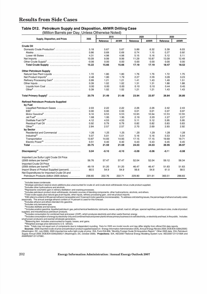
7/28/2019 2007 Annual Energy Outlook
http://slidepdf.com/reader/full/2007-annual-energy-outlook 211/243
202 Energy Information Administration / Annual Energy Outlook 2007
Results from Side Cases
Table D12. Petroleum Supply and Disposition, ANWR Drilling Case(Million Barrels per Day, Unless Otherwise Noted)
Supply, Disposition, and Prices 20052010 2020 2030
Reference ANWR Reference ANWR Reference ANWR
Crude Oil
Domestic Crude Production1 . . . . . . . . . . . . . . . . . . 5.18 5.67 5.67 5.89 6.32 5.39 6.03
Alaska . . . . . . . . . . . . . . . . . . . . . . . . . . . . . . . . . . 0.86 0.69 0.69 0.74 1.15 0.27 0.92
Lower 48 States . . . . . . . . . . . . . . . . . . . . . . . . . . 4.31 4.98 4.98 5.15 5.16 5.12 5.11
Net Imports . . . . . . . . . . . . . . . . . . . . . . . . . . . . . . . 10.09 9.99 9.99 11.29 10.87 13.09 12.49
Other Crude Supply2 . . . . . . . . . . . . . . . . . . . . . . . . -0.06 0.00 0.00 0.00 0.00 0.00 0.00
Total Crude Supply . . . . . . . . . . . . . . . . . . . . . . 15.22 15.66 15.66 17.19 17.19 18.47 18.52
Other Petroleum Supply
Natural Gas Plant Liquids . . . . . . . . . . . . . . . . . . . . 1.72 1.80 1.80 1.76 1.79 1.72 1.75
Net Product Imports3 . . . . . . . . . . . . . . . . . . . . . . . . 2.48 1.80 1.79 2.27 2.26 3.28 3.23
Refinery Processing Gain4 . . . . . . . . . . . . . . . . . . . 0.99 1.21 1.21 1.41 1.43 1.49 1.51
Other Inputs . . . . . . . . . . . . . . . . . . . . . . . . . . . . . . . 0.39 1.02 1.02 1.31 1.31 1.88 1.88
Liquids from Coal . . . . . . . . . . . . . . . . . . . . . . . . . 0.00 0.00 0.00 0.10 0.10 0.44 0.45
Other5 . . . . . . . . . . . . . . . . . . . . . . . . . . . . . . . . . . 0.39 1.02 1.02 1.21 1.21 1.43 1.43
Total Primary Supply6 . . . . . . . . . . . . . . . . . . . . . . . 20.79 21.49 21.48 23.94 23.97 26.84 26.89
Refined Petroleum Products Suppliedby Fuel
Liquefied Petroleum Gases . . . . . . . . . . . . . . . . . 2.03 2.22 2.22 2.26 2.26 2.42 2.43
E857 . . . . . . . . . . . . . . . . . . . . . . . . . . . . . . . . . . . 0.00 0.00 0.00 0.01 0.01 0.02 0.02
Motor Gasoline8 . . . . . . . . . . . . . . . . . . . . . . . . . . 9.16 9.53 9.53 10.93 10.94 12.53 12.55
Jet Fuel9 . . . . . . . . . . . . . . . . . . . . . . . . . . . . . . . . 1.68 1.95 1.95 2.19 2.20 2.27 2.27
Distillate Fuel Oil10 . . . . . . . . . . . . . . . . . . . . . . . . 4.12 4.53 4.53 5.11 5.12 5.95 5.95
Residual Fuel Oil . . . . . . . . . . . . . . . . . . . . . . . . . 0.92 0.79 0.79 0.82 0.82 0.83 0.83
Other11 . . . . . . . . . . . . . . . . . . . . . . . . . . . . . . . . . 2.84 2.57 2.57 2.70 2.69 2.93 2.92
by Sector
Residential and Commercial . . . . . . . . . . . . . . . . 1.26 1.25 1.25 1.29 1.29 1.28 1.28
Industrial12 . . . . . . . . . . . . . . . . . . . . . . . . . . . . . . 5.07 5.01 5.01 5.16 5.16 5.53 5.54
Transportation . . . . . . . . . . . . . . . . . . . . . . . . . . . 13.87 14.93 14.93 17.15 17.15 19.69 19.71
Electric Power13 . . . . . . . . . . . . . . . . . . . . . . . . . . 0.51 0.40 0.40 0.43 0.43 0.45 0.45
Total . . . . . . . . . . . . . . . . . . . . . . . . . . . . . . . . . . . . 20.75 21.59 21.59 24.03 24.03 26.95 26.97
Discrepancy14 . . . . . . . . . . . . . . . . . . . . . . . . . . . . . . 0.04 -0.10 -0.10 -0.09 -0.06 -0.11 -0.08
Imported Low Sulfur Light Crude Oil Price
(2005 dollars per barrel)15 . . . . . . . . . . . . . . . . . . . . . 56.76 57.47 57.47 52.04 52.04 59.12 58.34
Imported Crude Oil Price(2005 dollars per barrel)15 . . . . . . . . . . . . . . . . . . . . . 49.19 51.20 51.20 46.47 46.47 51.63 51.63
Import Share of Product Supplied (percent) . . . . . . . . 60.5 54.9 54.9 56.6 54.8 61.0 58.5
Net Expenditures for Imported Crude Oil and
Petroleum Products (billion 2005 dollars) . . . . . . . . 236.65 222.76 222.71 229.80 221.61 300.51 288.83
1Includes lease condensate.2Strategic petroleum reserve stock additions plus unaccounted for crude oil and crude stock withdrawals minus crude product supplied.3Includes other hydrocarbons and alcohols.4Represents volumetric gain in refinery distillation and cracking processes.5Includes petroleum product stock withdrawals; domestic sources of blending components, other hydrocarbons, alcohols, and ethers.6Total crude supply plus natural gas plant liquids, other inputs, refinery processing gain, and net product imports.7E85 refers to a blend of 85 percent ethanol (renewable) and 15 percent motor gasoline (nonrenewable). To address cold starting issues, the percentage of ethanol actually varies
seasonally. The annual average ethanol content of 74 percent is used for this forecast.8Includes ethanol and ethers blended into gasoline.9Includes only kerosene type.10Includes distillate and kerosene.11Includes aviation gasoline, liquefied petroleum gas, petrochemical feedstocks, lubricants, waxes, asphalt, road oil, still gas, special naphthas, petroleum coke, crude oil product
supplied, and miscellaneous petroleum products.12Includes consumption for combined heat and power (CHP), which produces electricity and other useful thermal energy.13Includes consumption of energy by electricity-only and combined heat and power plants whose primary business is to sell electricity, or electricity and heat, to the public. Includes
small power producers and exempt wholesale generators.14Balancing item. Includes unaccounted for supply, losses, and gains.15Weighted average price delivered to U.S. refiners.Note: Totals may not equal sum of components due to independent rounding. Data for 2005 are model results and may differ slightly from official EIA data reports.Sources: 2005 imported crude oil price and petroleum product supplied based on: Energy Information Administration (EIA), Annual Energy Review 2005 , DOE/EIA-0384(2005)
(Washington, DC, July 2006). 2005 imported low sulfur light crude oil price: EIA, Form EIA-856, “Monthly Foreign Crude Oil Acquisition Report.” Other 2005 data: EIA, Petroleum Supply Annual 2005, DOE/EIA-0340(2005)/1 (Washington, DC, October 2006). Projections: EIA, AEO2007 National Energy Modeling System runs AEO2007.D112106A andANWR2007.D112706C.

7/28/2019 2007 Annual Energy Outlook
http://slidepdf.com/reader/full/2007-annual-energy-outlook 212/243
Energy Information Administration / Annual Energy Outlook 2007 203
Results from Side Cases
Table D13. Petroleum Supply and Disposition, Expanded Outer Continental Shelf Access Case
Supply, Disposition, and Prices 20052010 2020 2030
Reference OCS Access Reference OCS Access Reference OCS Access
Petroleum Supply
Crude Oil
Domestic Crude Production1
. . . . . . . . . . . . . . . . 5.18 5.67 5.67 5.89 5.98 5.39 5.55Alaska . . . . . . . . . . . . . . . . . . . . . . . . . . . . . . . . 0.86 0.69 0.69 0.74 0.74 0.27 0.27
Lower 48 States . . . . . . . . . . . . . . . . . . . . . . . . 4.31 4.98 4.98 5.15 5.23 5.12 5.28
Onshore . . . . . . . . . . . . . . . . . . . . . . . . . . . . . 2.89 2.93 2.93 2.94 2.94 2.92 2.91
Offshore . . . . . . . . . . . . . . . . . . . . . . . . . . . . . 1.42 2.05 2.05 2.21 2.30 2.20 2.36
Net Imports . . . . . . . . . . . . . . . . . . . . . . . . . . . . . . 10.09 9.99 9.99 11.29 11.28 13.09 12.97
Other Crude Supply2 . . . . . . . . . . . . . . . . . . . . . . -0.06 0.00 0.00 0.00 0.00 0.00 0.00
Total Crude Supply . . . . . . . . . . . . . . . . . . . . . 15.22 15.66 15.66 17.19 17.26 18.47 18.52
Other Petroleum Supply
Natural Gas Plant Liquids . . . . . . . . . . . . . . . . . . 1.72 1.80 1.80 1.76 1.78 1.72 1.76
Net Product Imports3 . . . . . . . . . . . . . . . . . . . . . . 2.48 1.80 1.80 2.27 2.24 3.28 3.27
Refinery Processing Gain4 . . . . . . . . . . . . . . . . . . 0.99 1.21 1.21 1.41 1.35 1.49 1.42
Other Inputs . . . . . . . . . . . . . . . . . . . . . . . . . . . . . 0.39 1.02 1.02 1.31 1.30 1.88 1.88
Liquids from Coal . . . . . . . . . . . . . . . . . . . . . . . 0.00 0.00 0.00 0.10 0.10 0.44 0.44
Other5 . . . . . . . . . . . . . . . . . . . . . . . . . . . . . . . . 0.39 1.02 1.02 1.21 1.21 1.43 1.44
Total Petroleum Supply6 . . . . . . . . . . . . . . . . . . . . 20.79 21.49 21.48 23.94 23.93 26.84 26.85
Natural Gas Prices
(2005 dollars per million Btu)
Henry Hub Spot Price . . . . . . . . . . . . . . . . . . . . . . 8.60 6.28 6.27 5.71 5.66 6.52 6.37
Average Lower 48 Wellhead Price11 . . . . . . . . . . 7.29 5.59 5.58 5.07 5.02 5.80 5.67
(2005 dollars per thousand cubic feet)
Average Lower 48 Wellhead Price11 . . . . . . . . . . 7.51 5.76 5.75 5.22 5.18 5.98 5.84
Natural Gas Supply (trillion cubic feet)
Dry Gas Production7 . . . . . . . . . . . . . . . . . . . . . . . 18.23 19.35 19.35 20.79 21.02 20.53 21.14Lower 48 Onshore . . . . . . . . . . . . . . . . . . . . . . . . 14.36 15.22 15.22 14.66 14.63 15.13 15.15
Associated-Dissolved . . . . . . . . . . . . . . . . . . . . 1.43 1.39 1.39 1.28 1.28 1.19 1.19Non-Associated . . . . . . . . . . . . . . . . . . . . . . . . . 12.93 13.83 13.84 13.38 13.35 13.94 13.96
Conventional . . . . . . . . . . . . . . . . . . . . . . . . . 4.94 5.27 5.27 4.30 4.29 3.75 3.70Unconventional . . . . . . . . . . . . . . . . . . . . . . . . 7.99 8.56 8.57 9.09 9.06 10.19 10.26
Lower 48 Offshore . . . . . . . . . . . . . . . . . . . . . . . . 3.41 3.88 3.88 4.09 4.35 3.25 3.84Associated-Dissolved . . . . . . . . . . . . . . . . . . . . 0.71 0.92 0.92 1.05 1.08 0.85 1.04Non-Associated . . . . . . . . . . . . . . . . . . . . . . . . . 2.69 2.96 2.96 3.04 3.27 2.40 2.80
Alaska . . . . . . . . . . . . . . . . . . . . . . . . . . . . . . . . . . 0.45 0.25 0.25 2.05 2.05 2.16 2.16Supplemental Natural Gas8 . . . . . . . . . . . . . . . . . . . 0.07 0.07 0.07 0.07 0.07 0.07 0.07
Net Imports . . . . . . . . . . . . . . . . . . . . . . . . . . . . . . 3.57 4.55 4.55 5.35 5.20 5.45 5.20Pipeline . . . . . . . . . . . . . . . . . . . . . . . . . . . . . . . . . 3.01 2.74 2.74 1.65 1.65 0.92 0.92Liquefied Natural Gas9 . . . . . . . . . . . . . . . . . . . . . 0.57 1.81 1.81 3.69 3.55 4.53 4.28
Total Natural Gas Supply10 . . . . . . . . . . . . . . . . . . 21.87 23.97 23.97 26.21 26.29 26.06 26.41
1Includes lease condensate.2Strategic petroleum reserve stock additions plus unaccounted for crude oil and crude stock withdrawals minus crude product supplied.3Includes other hydrocarbons and alcohols.4Represents volumetric gain in refinery distillation and cracking processes.5Includes petroleum product stock withdrawals; domestic sources of blending components, other hydrocarbons, alcohols, and ethers.6Total crude supply plus natural gas plant liquids, other inputs, refinery processing gain, and net product imports.7Marketed production (wet) minus extraction losses.8Synthetic natural gas, propane air, coke oven gas, refinery gas, biomass gas, air injected for Btu stabilization, and manufactured gas commingled and distributed with natural
gas.9Includes any natural gas regasified in the Bahamas and transported via pipeline to Florida.10Dry gas production plus supplemental natural gas and net imports.Note: Totals may not equal sum of components due to independent rounding. Data for 2005 are model results and may differ slightly from official EIA data reports.Sources: 2005 imported crude oil price and petroleum product supplied based on: Energy Information Administration (EIA), Annual Energy Review 2005 , DOE/EIA-0384(2005)
(Washington, DC, July 2006). 2005 imported low sulfur light crude oil price: EIA, Form EIA-856, “Monthly Foreign Crude Oil Acquisition Report.” Other 2005 data: EIA, Petroleum Supply Annual 2005, DOE/EIA-0340(2005)/1 (Washington, DC, October 2006). Projections: EIA, AEO2007 National Energy Modeling System runs AEO2007.D112106A andOCSACC.D112706A.

7/28/2019 2007 Annual Energy Outlook
http://slidepdf.com/reader/full/2007-annual-energy-outlook 213/243
204 Energy Information Administration / Annual Energy Outlook 2007
Results from Side Cases
Table D14. Ethanol Supply, Disposition, and Prices, Additional Ethanol Cases
Supply, Disposition, and Prices 2005
2015 2030
ReferenceLow CostEthanol
HighPrice
Low CostEthanol andHigh Price
ReferenceLow CostEthanol
HighPrice
Low CostEthanol andHigh Price
Ethanol Supply (billion gallons)
Domestic ProductionCorn Based . . . . . . . . . . . . . . . . . . . . . . . . . . . . . 3.9 11.1 11.1 11.1 12.0 13.6 11.5 14.2 22.3
Cellulose Based . . . . . . . . . . . . . . . . . . . . . . . . . . 0.0 0.2 0.2 0.2 0.3 0.2 3.9 0.6 10.1
Total Domestic Production . . . . . . . . . . . . . . . 3.9 11.4 11.4 11.4 12.3 13.8 15.4 14.8 32.5
Ethanol Imports . . . . . . . . . . . . . . . . . . . . . . . . . . . . 0.1 0.4 0.5 0.5 0.5 0.8 0.8 0.8 1.5
Total Ethanol Supply . . . . . . . . . . . . . . . . . . . . . 4.0 11.7 11.9 11.9 12.8 14.6 16.2 15.6 33.9
Ethanol Consumption (billion gallons)
Used in E851 . . . . . . . . . . . . . . . . . . . . . . . . . . . . . . 0.0 0.0 0.2 0.1 1.0 0.2 1.4 2.4 20.6
Used in Gasoline Blending . . . . . . . . . . . . . . . . . . . 4.0 11.7 11.7 11.8 11.9 14.4 14.8 13.2 13.3
Total Ethanol Consumption . . . . . . . . . . . . . . . 4.0 11.7 11.9 11.9 12.8 14.6 16.2 15.6 33.9
Total Motor Gasoline Consumption (billion gallons) . 140.4 156.1 156.9 146.0 146.3 192.1 195.9 160.5 154.3
Light-Duty Vehicle Energy Consumption
(quadrillion Btu) . . . . . . . . . . . . . . . . . . . . . . . . . . . . . 16.36 17.99 18.03 16.83 16.90 22.66 22.49 19.50 19.84
Ethanol Percent of Motor Gasoline Pool (percent)2 . . 2.9 7.5 7.5 8.1 8.7 7.6 8.2 9.5 18.6
Transportation Sector Indicators
Light-Duty Vehicle Miles Travelled (billion miles) . . 2655 3125 3124 2978 2976 4226 4219 3924 3899New Car Efficiency (miles per gallon)3 . . . . . . . . . . 30.0 32.4 32.5 33.2 33.1 33.7 33.6 36.2 35.8New Light Truck Efficiency (miles per gallon)3 . . . . 21.8 24.7 24.3 25.3 24.8 26.5 25.8 28.2 27.2Light-Duty Stock Efficiency (miles per gallon)4 . . . . 19.6 20.6 20.5 20.9 20.8 22.2 22.2 23.9 23.5
E85-Capable Vehicle Sales (thousands) . . . . . . . . 613 1819 13401 1576 12887 2030 17045 3778 16816
Total Vehicle Sales (thousands) . . . . . . . . . . . . . . . 16235 17268 17270 16838 16828 20187 20176 20076 20063
E85-Capable Vehicle Stock (millions) . . . . . . . . . . . 4 17 48 16 46 31 229 37 225
Total Vehicle Stock (millions) . . . . . . . . . . . . . . . . . 220 263 263 259 259 316 316 312 312
Energy Prices (2005 dollars)
(dollars per gallon)
Imported Low Sulfur Light Crude Oil Price5 . . . . . 1.35 1.19 1.19 1.89 1.89 1.41 1.41 2.38 2.38Imported Crude Oil Price5 . . . . . . . . . . . . . . . . . . 1.17 1.06 1.06 1.76 1.76 1.23 1.23 2.21 2.21Transportation Sector Motor Gasoline6 . . . . . . . . 2.32 1.95 1.95 2.69 2.70 2.15 2.17 3.20 3.23E851 . . . . . . . . . . . . . . . . . . . . . . . . . . . . . . . . . . . 2.17 1.87 1.88 2.08 2.12 2.00 1.91 2.38 2.49Ethanol Wholesale Price . . . . . . . . . . . . . . . . . . . 1.80 1.66 1.68 1.70 1.75 1.70 1.61 1.84 2.28
(dollars per million Btu)
Imported Low Sulfur Light Crude Oil Price5 . . . . . 9.50 8.34 8.35 13.31 13.31 9.89 9.89 16.75 16.76Imported Crude Oil Price5 . . . . . . . . . . . . . . . . . . 8.23 7.46 7.46 12.36 12.36 8.64 8.64 15.55 15.55Transportation Sector Motor Gasoline6 . . . . . . . . 18.64 16.06 16.10 22.19 22.31 17.76 17.85 26.42 26.68E851 . . . . . . . . . . . . . . . . . . . . . . . . . . . . . . . . . . . 23.10 20.09 20.18 22.32 22.74 21.50 20.53 25.54 26.74Ethanol Wholesale Price . . . . . . . . . . . . . . . . . . . 21.65 19.92 20.17 20.44 21.03 20.43 19.37 22.02 27.39
1E85 refers to a blend of 85 percent ethanol (renewable) and 15 percent motor gasoline (nonrenewable). To address cold starting issues, the percentage of ethanol actually variesseasonally. The annual average ethanol content of 74 percent is used for this forecast.
2Calculated as the amount of ethanol consumed divided by the total amount of ethanol and motor gasoline consumed.3Environmental Protection Agency rated miles per gallon.4Combined car and light truck “on-the-road” estimate.5Weighted average price delivered to U.S. refiners.6Sales weighted average price for all grades. Includes Federal, State, and local taxes.Note: Totals may not equal sum of components due to independent rounding. Data for 2005 are model results and may differ slightly from official EIA data reports.
Sources: 2005 consumption and imported crude oil price: Energy Information Administration (EIA), Annual Energy Review 2005 , DOE/EIA-0384(2005) (Washington, DC, July2006). 2005 imported low sulfur light crude oil price: EIA, Form EIA-856, “Monthly Foreign Crude Oil Acquisition Report.” 2005 motor gasoline price based on: EIA, Petroleum Marketing Annual 2005 , DOE/EIA-0487(2005) (Washington, DC, August 2006). 2005 ethanol prices derived from weekly spot prices in the Oxy Fuel News. 2005 wholesale ethanolprices derived from Bloomburg U.S. average rack price. Projections: EIA, AEO2007 National Energy Modeling System runs AEO2007.D112106A, CT_80PCT_7L_RF.D120406A,HP2007.D112106A, and CT_80PCT_7L.D120406A.

7/28/2019 2007 Annual Energy Outlook
http://slidepdf.com/reader/full/2007-annual-energy-outlook 214/243
Energy Information Administration / Annual Energy Outlook 2007 205
Results from Side Cases
Table D15. Key Results for Coal Cost Cases(Million Short Tons per Year, Unless Otherwise Noted)
Supply, Disposition, and Prices 20052015 2030 Growth Rate, 2005-2030
Low Cost Reference High Cost Low Cost Reference High Cost Low Cost Reference High Cost
Production1 . . . . . . . . . . . . . . . . . . . . . . . . 1131 1278 1266 1209 1824 1691 1329 1.9% 1.6% 0.6%
Appalachia . . . . . . . . . . . . . . . . . . . . . . . . 397 381 371 349 420 373 337 0.2% -0.3% -0.7%Interior . . . . . . . . . . . . . . . . . . . . . . . . . . . 149 188 199 204 275 247 255 2.5% 2.0% 2.2%
West . . . . . . . . . . . . . . . . . . . . . . . . . . . . 585 709 697 656 1129 1072 736 2.7% 2.5% 0.9%
Waste Coal Supplied2 . . . . . . . . . . . . . . . . 13 14 13 13 9 13 17 -1.8% -0.0% 0.9%
Net Imports . . . . . . . . . . . . . . . . . . . . . . . . -21 3 5 18 47 68 83 N/A N/A N/A
Total Supply3 . . . . . . . . . . . . . . . . . . . . . . . 1124 1294 1284 1239 1880 1772 1428 2.1% 1.8% 1.0%
Consumption by Sector
Residential and Commercial . . . . . . . . . . 5 5 5 5 5 5 5 -0.3% -0.3% -0.3%
Coke Plants . . . . . . . . . . . . . . . . . . . . . . . 23 21 21 21 21 21 20 -0.4% -0.5% -0.6%
Other Industrial4 . . . . . . . . . . . . . . . . . . . . 61 63 62 62 64 64 63 0.2% 0.2% 0.1%
Coal-to-Liquids Heat and Power . . . . . . . 0 9 8 3 65 57 16 N/A N/A N/A
Coal-to-Liquids Liquids Production . . . . . 0 9 8 3 63 55 15 N/A N/A N/A
Electric Power5 . . . . . . . . . . . . . . . . . . . . 1039 1186 1178 1146 1662 1570 1310 1.9% 1.7% 0.9%
Total Coal Use . . . . . . . . . . . . . . . . . . 1128 1293 1282 1239 1880 1772 1428 2.1% 1.8% 0.9%
Average Minemouth Price6
(2005 dollars per short ton) . . . . . . . . . . . 23.34 18.68 22.41 27.12 14.30 22.60 41.01 -1.9% -0.1% 2.3%(2005 dollars per million Btu) . . . . . . . . . 1.15 0.92 1.11 1.35 0.72 1.15 2.05 -1.9% -0.0% 2.3%
Delivered Prices7
(2005 dollars per short ton)
Coke Plants . . . . . . . . . . . . . . . . . . . . . . . 83.79 66.66 74.51 84.52 57.27 75.55 111.24 -1.5% -0.4% 1.1%
Other Industrial4 . . . . . . . . . . . . . . . . . . . . 47.63 43.03 47.45 52.26 38.01 48.54 65.93 -0.9% 0.1% 1.3%
Coal to Liquids . . . . . . . . . . . . . . . . . . . . . N/A 11.23 13.79 17.09 15.10 21.89 31.59 N/A N/A N/A
Electric Power5
(2005 dollars per short ton) . . . . . . . . . 30.83 28.37 31.84 36.37 24.63 33.52 49.75 -0.9% 0.3% 1.9%
(2005 dollars per million Btu) . . . . . . . . 1.53 1.42 1.60 1.83 1.23 1.69 2.49 -0.9% 0.4% 2.0%
Average . . . . . . . . . . . . . . . . . . . . . 32.82 29.47 33.10 37.91 24.80 33.82 50.93 -1.1% 0.1% 1.8%
Exports8 . . . . . . . . . . . . . . . . . . . . . . . . . . 67.10 58.08 64.51 73.77 51.47 63.81 95.87 -1.1% -0.2% 1.4%
Cumulative Electricity GeneratingCapacity Additions (gigawatts)9
Coal . . . . . . . . . . . . . . . . . . . . . . . . . . . . . 0.0 22.6 19.5 15.7 189.2 156.3 77.0 N/A N/A N/A
Conventional: Pulverized Coal . . . . . . . 0.0 17.9 15.8 12.9 111.5 78.4 44.4 N/A N/A N/A
Advanced: IGCC . . . . . . . . . . . . . . . . . 0.0 4.7 3.6 2.7 77.7 77.9 32.6 N/A N/A N/A
Petroleum . . . . . . . . . . . . . . . . . . . . . . . . 0.0 0.2 0.2 0.2 0.3 0.3 0.3 N/A N/A N/A
Natural Gas . . . . . . . . . . . . . . . . . . . . . . . 0.0 32.3 33.1 33.7 92.7 105.2 133.1 N/A N/A N/A
Nuclear . . . . . . . . . . . . . . . . . . . . . . . . . . 0.0 1.8 0.5 1.3 6.0 12.5 42.3 N/A N/A N/A
Renewables 10 . . . . . . . . . . . . . . . . . . . . . 0.0 10.7 10.8 10.9 15.5 17.5 20.8 N/A N/A N/A
Other . . . . . . . . . . . . . . . . . . . . . . . . . . . . 0.0 0.1 0.1 0.1 0.1 0.2 0.2 N/A N/A N/A
Total . . . . . . . . . . . . . . . . . . . . . . . . . . . 0.0 67.7 64.2 61.9 303.8 291.9 273.7 N/A N/A N/A
Liquids from Coal (million barrels per day) 0.00 0.07 0.06 0.02 0.51 0.44 0.12 N/A N/A N/A
Labor Productivity
Coal Mining(short tons per miner per hour) . . . . . . . . 6.36 8.72 6.80 5.25 14.77 7.84 3.38 3.4% 0.8% -2.5%
Rail: Eastern Railroads (billion freightton-miles per employee per year) . . . . . . 7.57 10.90 8.91 7.25 18.17 10.61 6.11 3.6% 1.4% -0.9%
Rail: Western Railroads (billion freightton-miles per employee per year) . . . . . . 12.19 17.72 14.49 11.79 29.86 17.43 10.05 3.6% 1.4% -0.8%

7/28/2019 2007 Annual Energy Outlook
http://slidepdf.com/reader/full/2007-annual-energy-outlook 215/243
206 Energy Information Administration / Annual Energy Outlook 2007
Results from Side Cases
Table D15. Key Results for Coal Cost Cases (Continued)(Million Short Tons per Year, Unless Otherwise Noted)
Supply, Disposition, and Prices 20052015 2030 Growth Rate, 2005-2030
Low Cost Reference High Cost Low Cost Reference High Cost Low Cost Reference High Cost
Cost Indices(constant dollar index, 2005=1.000)
Transportation Rate Multipliers
Eastern Railroads . . . . . . . . . . . . . . . . . 1.000 1.043 1.064 1.086 0.968 1.042 1.121 -0.1% 0.2% 0.5%
Western Railroads . . . . . . . . . . . . . . . . 1.000 1.029 1.046 1.063 0.971 1.028 1.088 -0.1% 0.1% 0.3%
Equipment Costs
Mining
Underground . . . . . . . . . . . . . . . . . . . 1.000 0.943 1.032 1.129 0.811 1.032 1.311 -0.8% 0.1% 1.1%
Surface . . . . . . . . . . . . . . . . . . . . . . . 1.000 0.927 1.016 1.110 0.798 1.016 1.289 -0.9% 0.1% 1.0%
Railroads . . . . . . . . . . . . . . . . . . . . . . . 1.000 0.905 0.991 1.085 0.743 0.946 1.202 -1.2% -0.2% 0.7%
Average Coal Miner Wage(2005 dollars per hour) . . . . . . . . . . . . . . . 22.06 20.16 22.06 24.13 17.34 22.06 28.02 -1.0% -0.0% 1.0%
1Includes anthracite, bituminous coal, and lignite.2Includes waste coal consumed by the electric power and industrial sectors. Waste coal supplied is counted as a supply-side item to balance the same amount of waste coal
included in the consumption data.3Production plus net imports plus net storage withdrawals.4Includes consumption for combined heat and power plants, except those plants whose primary business is to sell electricity, or electricity and heat, to the public. Excludes all
coal use in the coal to liquids process.5Includes all electricity-only and combined heat and power plants whose primary business is to sell electricity, or electricity and heat, to the public.6Includes reported prices for both open market and captive mines.7Prices weighted by consumption tonnage; weighted average excludes residential and commercial prices, and export free-alongside-ship (f.a.s.) prices.8F.a.s. price at U.S. port of exit.9Cumulative additions after December 31, 2005. Includes all additions of electricity only and combined heat and power plants projected for the electric power, industrial, and
commercial sectors.10Includes conventional hydroelectric, geothermal, wood, wood waste, municipal solid waste, landfill gas, other biomass, solar, and wind power. Facilities co-firing biomass and
coal are classified as coal.N/A = Not applicable.Btu = British thermal unit.IGCC = Integrated gas combined cycle.Note: Totals may not equal sum of components due to independent rounding. Data for 2005 are model results and may differ slightly from official EIA data reports.Sources: 2005 data based on: Energy Information Administration (EIA),Annual Coal Report 2005 , DOE/EIA-0584(2005) (Washington, DC, October 2006); EIA, Quarterly Coal
Report, October-December 2005 , DOE/EIA-0121(2005/4Q) (Washington, DC, March 2006); Securities and Exchange Commission Form 10K fil ings (BNSF, Norfolk Southern, andUnion Pacific), web site www.sec.gov; CSX Corporation, web site www.csx.com; U.S. Department of Labor, Bureau of Labor Statistics, Average Hourly Earnings of ProductionWorkers: Coal Mining, Series ID : ceu1021210006; and EIA, AEO2007 National Energy Modeling System run AEO2007.D112106A. Projections: EIA, AEO2007 National EnergyModeling System runs LCCST07.D112906A, AEO2007.D112106A, and HCCST07.D112906A.

7/28/2019 2007 Annual Energy Outlook
http://slidepdf.com/reader/full/2007-annual-energy-outlook 216/243
The National Energy Modeling System
The projections in the Annual Energy Outlook 2007
( AEO2007 ) are generated from the National EnergyModeling System (NEMS) [1], developed and main-
tained by the Office of Integrated Analysis and
Forecasting (OIAF) of the Energy Information Ad-
ministration (EIA). In addition to its use in the devel-
opment of the AEO projections, NEMS is also used
in analytical studies for the U.S. Congress, the White
House, and other offices within the Department of
Energy. The AEO projections are also used by ana-
lysts and planners in other government agencies and
outside organizations.
The projections in NEMS are developed with the use
of a market-based approach to energy analysis. Foreach fuel and consuming sector, NEMS balances
energy supply and demand, accounting for economic
competition among the various energy fuels and
sources. The time horizon of NEMS is the long-term
period through 2030, approximately 25 years into the
future. In order to represent regional differences in
energy markets, the component modules of NEMS
function at the regional level: the nine Census divi-
sions for the end-use demand modules; production re-
gions specific to oil, natural gas, and coal supply and
distribution; the North American Electric Reliability
Council regions and subregions for electricity; andthe Petroleum Administration for Defense Districts
(PADDs) for refineries.
NEMS is organized and implemented as a modular
system. The modules represent each of the fuel sup-
ply markets, conversion sectors, and end-use con-
sumption sectors of the energy system. NEMS also
includes macroeconomic and international modules.
The primary flows of information among the modules
are the delivered prices of energy to end users and the
quantities consumed by product, region, and sector.
The delivered fuel prices encompass all the activities
necessary to produce, import, and transport fuels toend users. The information flows also include other
data on such areas as economic activity, domestic pro-
duction, and international petroleum supply.
The Integrating Module controls the execution of
each of the component modules. To facilitate modu-
larity, the components do not pass information to
each other directly but communicate through a
central data structure. This modular design provides
the capability to execute modules individually, thus
allowing decentralized development of the system
and independent analysis and testing of individual
modules, and permits the use of the methodologyand level of detail most appropriate for each energy
sector. NEMS calls each supply, conversion, and
end-use demand module in sequence until the deliv-
ered prices of energy and the quantities demanded
have converged within tolerance, thus achieving an
economic equilibrium of supply and demand in the
consuming sectors. A solution is reached annually
through the long-term horizon. Other variables are
also evaluated for convergence, such as petroleum
product imports, crude oil imports, and several mac-
roeconomic indicators.
Each NEMS component represents the impacts and
costs of legislation and environmental regulations
that affect that sector. NEMS accounts for all com-
bustion-related carbon dioxide (CO2) emissions, as
well as emissions of sulfur dioxide, nitrogen oxides,
and mercury from the electricity generation sector.
NEMS generally represents current legislation and
environmental regulations as of October 31, 2006
(such as the Energy Policy Acts of 2005 [EPACT-
2005], the Working Families Tax Relief Act of 2004,
and the American Jobs Creation Act of 2004) and the
costs of compliance with regulations such as the
Clean Air Interstate Rule (CAIR) and Clean Air Mer-
cury Rule (CAMR), both of which were finalized and
published in 2005, the new corporate average fuel
economy (CAFE) standards finalized in March 2006,
and the new stationary diesel regulations issued by
the U.S. Environmental Protection Agency (EPA) in
July 2006. The potential impacts of pending or pro-
posed Federal and State legislation, regulations, or
standards—or of sections of legislation that have
been enacted but that require funds or implementing
regulations that have not been provided or speci-
fied—are not reflected in NEMS.
In general, the historical data used for the AEO2007
projections were based on EIA’s Annual Energy Re-
view 2005 , published in July 2006 [ 2]; however, data
were taken from multiple sources. In some cases, only
partial or preliminary data were available for 2005.
CO2 emissions were calculated by using CO2 coeffi-
cients from the EIA report, Emissions of Greenhouse
Gases in the United States 2005 , published in Novem-
ber 2006 [3].
Appendix E
NEMS Overview and Brief Description of Cases
Energy Information Administration / Annual Energy Outlook 2007 207

7/28/2019 2007 Annual Energy Outlook
http://slidepdf.com/reader/full/2007-annual-energy-outlook 217/243
Historical numbers are presented for comparison
only and may be estimates. Source documents should
be consulted for the official data values. Footnotes to
the AEO2007 appendix tables indicate the definitions
and sources of historical data.
The AEO2007 projections for years 2006 and 2007 in-
corporate short-term projections from EIA’s Septem-
ber 2006 Short-Term Energy Outlook (STEO). For
short-term energy projections, readers are referred to
monthly updates of the STEO [ 4].
Component Modules
The component modules of NEMS represent the indi-
vidual supply, demand, and conversion sectors of
domestic energy markets and also include interna-
tional and macroeconomic modules. In general, the
modules interact through values representing theprices or expenditures of energy delivered to the con-
suming sectors and the quantities of end-use energy
consumption.
Macroeconomic Activity Module
The Macroeconomic Activity Module provides a set of
macroeconomic drivers to the energy modules, and
there is a macroeconomic feedback mechanism within
NEMS. Key macroeconomic variables used in the en-
ergy modules include gross domestic product (GDP),
disposable income, industrial output, new housing
starts, new light-duty vehicle sales, interest rates,prices, and employment. The module uses the follow-
ing models from Global Insight, Inc. (GII): Macroeco-
nomic Model of the U.S. Economy, National Industry
Model, and National Employment Model. In addition,
EIA has constructed a Regional Economic and Indus-
try Model to project regional economic drivers and a
Commercial Floorspace Model to project 13 floorspace
types in 9 Census divisions. The accounting frame-
work for industrial output uses the North American
Industry Classification System (NAICS).
International Module
The International Module represents the response of
world oil markets (supply and demand) to assumed
world oil prices. The results/outputs of the module
are a set of crude oil and product supply curves that
are available to U.S. markets for each case/scenario
analyzed. The petroleum import supply curves are
made available to U.S. markets through the Petro-
leum Market Module (PMM) of NEMS in the form of
5 categories of imported crude oil and 17 interna-
tional petroleum products, including supply curves
for oxygenates and unfinished oils. The supply-curve
calculations are based on historical market data and a
world oil supply/demand balance, which is developed
from the International Energy Outlook 2006, current
investment trends in exploration and development,
and long-term resource economics for 221 coun-tries/territories. The oil production estimates include
both conventional and unconventional supply recov-
ery technologies.
Residential and Commercial Demand Modules
The Residential Demand Module projects energy con-
sumption in the residential sector by housing type
and end use, based on delivered energy prices, the
menu of equipment available, the availability of re-
newable sources of energy, and housing starts. The
Commercial Demand Module projects energy con-
sumption in the commercial sector by building typeand nonbuilding uses of energy and by category of end
use, based on delivered prices of energy, availability of
renewable sources of energy, and macroeconomic
variables representing interest rates and floorspace
construction.
Both modules estimate the equipment stock for the
major end-use services, incorporating assessments of
advanced technologies, including representations of
renewable energy technologies and the effects of both
building shell and appliance standards. The Commer-
cial Demand Module incorporates combined heat andpower (CHP) technology. The modules also include
projections of distributed generation. Both modules
incorporate changes to “normal” heating and cooling
degree-days by Census division, based on State-level
population projections. The Residential Demand
Module projects that the average square footage of
both new construction and existing structures is in-
creasing, based on trends in the size of new construc-
tion and the remodeling of existing homes.
Industrial Demand Module
The Industrial Demand Module projects the con-sumption of energy for heat and power and for feed-
stocks and raw materials in each of 21 industries,
subject to the delivered prices of energy and macro-
economic variables representing employment and the
value of shipments for each industry. As noted in the
description of the Macroeconomic Activity Module,
the value of shipments is based on NAICS. The
industries are classified into three groups—energy-
intensive manufacturing, non-energy-intensive man-
ufacturing, and nonmanufacturing. Of the 8 energy-
208 Energy Information Administration / Annual Energy Outlook 2007
NEMS Overview and Brief Description of Cases

7/28/2019 2007 Annual Energy Outlook
http://slidepdf.com/reader/full/2007-annual-energy-outlook 218/243
intensive industries, 7 are modeled in the Industrial
Demand Module, with components for boiler/steam/
cogeneration, buildings, and process/assembly use of
energy. Bulk chemicals are further disaggregated to
organic, inorganic, resins, and agricultural chemicals.
A representation of cogeneration and a recycling com-ponent are also included. The use of energy for petro-
leum refining is modeled in the PMM, and the pro-
jected consumption is included in the industrial
totals.
Transportation Demand Module
The Transportation Demand Module projects con-
sumption of fuels in the transportation sector, in-
cluding petroleum products, electricity, methanol,
ethanol, compressed natural gas, and hydrogen, by
transportation mode, vehicle vintage, and size class,
subject to delivered prices of energy fuels and macro-economic variables representing disposable personal
income, GDP, population, interest rates, and indus-
trial shipments. Fleet vehicles are represented sepa-
rately to allow analysis of the Clean Air Act Amend-
ments of 1990 (CAAA90) and other legislation and
legislative proposals. The module also includes a com-
ponent to assess the penetration of alternative-fuel
vehicles.
The air transportation component explicitly repre-
sents the industry practice of parking aircraft to re-
duce operating costs and the movement of aircraftfrom passenger to cargo markets as aircraft age [5 ].
For air freight shipments, the model represents fuel
use in narrow-body and wide-body aircraft. An infra-
structure constraint limits overall growth in passen-
ger and freight air travel to levels commensurate with
industry-projected infrastructure expansion and ca-
pacity growth.
Electricity Market Module
The Electricity Market Module represents genera-
tion, transmission, and pricing of electricity, subject
to delivered prices for coal, petroleum products, natu-ral gas, and biofuels; costs of generation by all genera-
tion plants, including capital costs; macroeconomic
variables for costs of capital and domestic invest-
ment; enforced environmental emissions laws and
regulations; and electricity load shapes and demand.
There are three primary submodules—capacity plan-
ning, fuel dispatching, and finance and pricing.
Nonutility generation, distributed generation, and
transmission and trade are modeled in the planning
and dispatching submodules.
All specifically identified CAAA90 compliance options
that have been promulgated by the EPA are explicitly
represented in the capacity expansion and dispatch
decisions; those that have not been promulgated (e.g.,
fine particulate proposals) are not incorporated. All
financial incentives for power generation expansionand dispatch specifically identified in EPACT2005
have been implemented. Several States, primarily in
the Northeast, have recently enacted air emission
regulations that affect the electricity generation sec-
tor. Where firm State compliance plans have been an-
nounced, regulations are represented in AEO2007 .
Renewable Fuels Module
The Renewable Fuels Module (RFM) includes sub-
modules representing renewable resource supply and
technology input information for central-station,
grid-connected electricity generation technologies,
including conventional hydroelectricity, biomass
(wood, energy crops, and biomass co-firing), geo-
thermal, landfill gas, solar thermal electricity, solar
photovoltaics (PV), and wind energy. The RFM con-
tains renewable resource supply estimates represent-
ing the regional opportunities for renewable energy
development. Investment tax credits for renewable
fuels are incorporated, as currently legislated in
the Energy Policy Act of 1992 (EPACT1992) and
EPACT2005. EPACT1992 provides a 10-percent tax
credit for business investment in solar energy (ther-
mal non-power uses as well as power uses) and geo-thermal power; those credits have no expiration date.
EPACT2005 increases the tax credit to 30 percent for
solar energy systems installed before January 1, 2008
(which has since been extended to January 1, 2009,
but is not reflected in the AEO2007 projections).
Production tax credits for wind, geothermal, landfill
gas, and some types of hydroelectric and biomass-
fueled plants are also represented. They provide a tax
credit of up to 1.9 cents per kilowatthour for electric-
ity produced in the first 10 years of plant operation.
At the time AEO2007 was completed, new plantscoming on line before January 1, 2008, were eligible
to receive the credit. Subsequently—after AEO2007
modeling runs were completed—the deadline was ex-
tended to January 1, 2009. Significant changes made
for AEO2007 in the accounting of new renewable en-
ergy capacity resulting from State renewable portfo-
lio standard (RPS) programs, mandates, and goals are
described in Assumptions to the Annual Energy Out-
look 2007 [6].
NEMS Overview and Brief Description of Cases
Energy Information Administration / Annual Energy Outlook 2007 209

7/28/2019 2007 Annual Energy Outlook
http://slidepdf.com/reader/full/2007-annual-energy-outlook 219/243
Oil and Gas Supply Module
The Oil and Gas Supply Module represents domestic
crude oil and natural gas supply within an integrated
framework that captures the interrelationships
among the various sources of supply: onshore, off-
shore, and Alaska by both conventional and uncon-
ventional techniques, including natural gas recovery
from coalbeds and low-permeability formations of
sandstone and shale. This framework analyzes cash
flow and profitability to compute investment and
drilling for each of the supply sources, based on the
prices for crude oil and natural gas, the domestic re-
coverable resource base, and the state of technology.
Oil and gas production functions are computed at a
level of 12 supply regions, including 3 offshore and 3
Alaskan regions. The module also represents foreign
sources of natural gas, including pipeline imports and
exports to Canada and Mexico, and liquefied naturalgas (LNG) imports and exports.
Crude oil production quantities are input to the PMM
in NEMS for conversion and blending into refined
petroleum products. Supply curves for natural gas are
input to the Natural Gas Transmission and Distribu-
tion Module for use in determining natural gas prices
and quantities. International LNG supply sources
and options for construction of new regasification ter-
minals in Canada, Mexico, and the United States as
well as expansions of existing U.S. regasification ter-
minals are represented, based on the projected re-
gional costs associated with international natural gas
supply, liquefaction, transportation, and regasifica-
tion and world natural gas market conditions.
Natural Gas Transmission and Distribution
Module
The Natural Gas Transmission and Distribution
Module represents the transmission, distribution,
and pricing of natural gas, subject to end-use demand
for natural gas and the availability of domestic natu-
ral gas and natural gas traded on the international
market. The module tracks the flows of natural gas
and determines the associated capacity expansion re-quirements in an aggregate pipeline network, con-
necting the domestic and foreign supply regions with
12 demand regions. The flow of natural gas is deter-
mined for both a peak and off-peak period in the year.
Key components of pipeline and distributor tariffs are
included in separate pricing algorithms.
Petroleum Market Module
The PMM projects prices of petroleum products,
crude oil and product import activity, and domestic
refinery operations (including fuel consumption),
subject to the demand for petroleum products, the
availability and price of imported petroleum, and the
domestic production of crude oil, natural gas liquids,
and alcohol and biodiesel fuels. The module repre-
sents refining activities in the five PADDs. It explic-itly models the requirements of CAAA90 and the
costs of automotive fuels, such as conventional and
reformulated gasoline, and includes biofuels produc-
tion for blending in gasoline and diesel.
AEO2007 represents the nationwide phase-in of gaso-
line with an annual average sulfur content of 30 ppm
between 2005 and 2007, regulations that limit the
sulfur content of highway diesel fuel to 15 ppm start-
ing in mid-2006 and of all non-road and locomo-
tive/marine diesel to 15 ppm by mid-2012, and the re-
newable fuels standard of 7.5 billion gallons by 2012.Demand growth and regulatory changes necessitate
capacity expansion for refinery processing units. For
those investments, a financing ratio of 60 percent eq-
uity and 40 percent debt is assumed, with a hurdle
rate and an after-tax return on investment of about 9
percent [7 ]. End-use prices are based on the marginal
costs of production, plus markups representing prod-
uct marketing and distribution costs and State and
Federal taxes [8]. Refinery capacity expansion at ex-
isting sites is permitted in all five refining regions
modeled. AEO2007 accounts for the phasing out of
methyl tertiary butyl ether (MTBE) as a result of de-
cisions made by the petroleum industry to discon-
tinue MTBE blending with gasoline.
Fuel ethanol and biodiesel are included in the PMM,
because they are commonly blended into petroleum
products. The module allows ethanol blending into
gasoline at 10 percent by volume or less, as well as
E85, a blend of up to 85 percent ethanol by volume.
Ethanol is produced primarily in the Midwest from
corn or other starchy crops, and it is expected to be
produced from cellulosic material in other regions in
the future. Biodiesel is produced from soybean oil or
yellow grease (primarily, recycled cooking oil). Bothsoybean oil biodiesel and yellow grease biodiesel are
assumed to be blended into highway diesel.
Alternative fuels such as coal-to-liquids (CTL) and
gas-to-liquids (GTL) are modeled in the PMM, based
on their economics relative to competing feedstocks
and products. CTL facilities are likely to be built at lo-
cations close to coal supply and water sources, where
liquid products and electricity could also be distrib-
uted to nearby demand regions. GTL facilities may be
210 Energy Information Administration / Annual Energy Outlook 2007
NEMS Overview and Brief Description of Cases

7/28/2019 2007 Annual Energy Outlook
http://slidepdf.com/reader/full/2007-annual-energy-outlook 220/243
built on the North Slope of Alaska but would compete
with the Alaska Natural Gas Transportation System
for available natural gas resources.
Ethanol production is modeled from two feedstocks:
corn and cellulosic materials such as switchgrass andpoplar. Corn-based ethanol plants are numerous
(more than 80 in operation, producing more than 4
billion gallons annually) and are based on a well-
known technology that converts sugars into ethanol.
Ethanol from cellulosic sources is a new technology
with no full-sized plants constructed. The two sources
are modeled to compete on an economic basis to meet
the EPACT2005 mandate.
Coal Market Module
The Coal Market Module (CMM) simulates mining,
transportation, and pricing of coal, subject to end-use
demand for coal differentiated by heat and sulfur con-
tent. U.S. coal production is represented in the CMM
by 40 separate supply curves—differentiated by re-
gion, mine type, coal rank, and sulfur content. The
coal supply curves include a response to capacity utili-
zation of mines, mining capacity, labor productivity,
and factor input costs (mining equipment, mining la-
bor, and fuel requirements). Projections of U.S. coal
distribution are determined by minimizing the cost of
coal supplied, given coal demands by demand region
and sector, accounting for minemouth prices, trans-
portation costs, existing coal supply contracts, and
sulfur and mercury allowance costs. Over the projec-tion horizon, coal transportation costs in the CMM
are projected to vary in response to changes in rail-
road productivity and the cost of rail transportation
equipment and diesel fuel.
The CMM produces projections of U.S. steam and
metallurgical coal exports and imports, in the context
of world coal trade. The CMM determines the pattern
of world coal trade flows that minimizes the produc-
tion and transportation costs of meeting a specified
set of regional world coal import demands, subject to
constraints on export capacities and trade flows. The
international coal market component of the module
computes trade in 3 types of coal for 17 export and 20
import regions. U.S. coal production and distribution
are computed for 14 supply and 14 demand regions.
Annual Energy Outlook 2007 Cases
Table E1 provides a summary of the cases used to de-
rive the AEO2007 projections. For each case, the table
gives the name used in this report, a brief description
of the major assumptions underlying the projections,
a designation of the mode in which the case was run in
NEMS (either fully integrated, partially integrated,
or standalone), and a reference to the pages in the
body of the report and in this appendix where the case
is discussed. The following sections describe the cases
listed in Table E1. The reference case assumptions foreach sector are described at web site www.eia.doe.
gov/oiaf/aeo/assumption. Regional results and other
details of the projections are available at web site
www.eia.doe.gov/oiaf/aeo/supplement.
Macroeconomic Growth Cases
In addition to the AEO2007 reference case, the low
economic growth and high economic growth cases
were developed to reflect the uncertainty in projec-
tions of economic growth. The alternative cases are
intended to show the effects of alternative growth as-
sumptions on energy market projections. The casesare described as follows:
The low economic growth case assumes lower
growth rates for population (0.5 percent per year),
non-farm employment (0.6 percent per year), and
productivity (1.9 percent per year), resulting in
higher prices and interest rates and lower growth
in industrial output. In the low economic growth
case, economic output as measured by real GDP
increases by 2.3 percent per year from 2005
through 2030, and growth in real GDP per capita
averages 1.8 percent per year.
• The high economic growth case assumes higher
growth rates for population (1.2 percent per year),
nonfarm employment (1.3 percent per year), and
productivity (2.8 percent per year). With higher
productivity gains and employment growth, infla-
tion and interest rates are lower than in the refer-
ence case, and consequently economic output
grows at a higher rate (3.4 percent per year) than
in the reference case (2.9 percent). GDP per capita
grows by 2.2 percent per year, compared with 2.1
percent in the reference case.
Price Cases
The world oil price in AEO2007 is defined as the aver-
age price of low-sulfur, light crude oil imported into
the United States. The low-sulfur, light crude oil price
is similar to prices for the light sweet crude oil con-
tract traded on the New York Mercantile Exchange.
AEO2007 also includes a projection of the U.S. annual
average imported refiners’ acquisition cost of crude
oil, whichis more representative of the average cost of
all crude oils used by refiners.
NEMS Overview and Brief Description of Cases
Energy Information Administration / Annual Energy Outlook 2007 211

7/28/2019 2007 Annual Energy Outlook
http://slidepdf.com/reader/full/2007-annual-energy-outlook 221/243
212 Energy Information Administration / Annual Energy Outlook 2007
NEMS Overview and Brief Description of Cases
Table E1. Summary of the AEO2007 cases
Case name Description
Integration
mode
Reference
in text
Reference in
Appendix E
Reference Baseline economic growth (2.9 percent per year from
2005 through 2030), world oil price, and technologyassumptions. Complete projection tables in Appendix A.
Fully
integrated
— —
Low Economic Growth Gross domestic product grows at an average annualrate of 2.3 percent from 2005 through 2030. Other assumptions are the same as in the reference case.Partial projection tables in Appendix B.
Fullyintegrated
p. 68 p. 211
High Economic Growth Gross domestic product grows at an average annualrate of 3.4 percent from 2005 through 2030. Other assumptions are the same as in the reference case.Partial projection tables in Appendix B.
Fullyintegrated
p. 68 p. 211
Low Price More optimistic assumptions for worldwide crude oil andnatural gas resources than in the reference case. Worldlight, sweet crude oil prices are $36 per barrel in 2030,
compared with $59 per barrel in the reference case(2005 dollars). Other assumptions are the same as inthe reference case. Partial projection tables in Appendix C.
Fullyintegrated
p. 34 p. 215
High Price More pessimistic assumptions for worldwide crude oiland natural gas resources than in the reference case.World light, sweet crude oil prices are about $100 per barrel in 2030. Other assumptions are the same as inthe reference case. Partial projection tables in Appendix C.
Fullyintegrated
p. 34 p. 215
Residential:2006 Technology
Future equipment purchases based on equipmentavailable in 2006. Existing building shell efficiencies fixedat 2006 levels. Partial projection tables in Appendix D.
Withcommercial
p. 74 p. 215
Residential:High Technology Earlier availability, lower costs, and higher efficienciesassumed for more advanced equipment. Building shellefficiencies for new construction meet ENERGY STARrequirements after 2010. Partial projection tables in Appendix D.
Withcommercial p. 74 p. 215
Residential:Best AvailableTechnology
Future equipment purchases and new building shellsbased on most efficient technologies available by fuel.Building shell efficiencies for new construction meetthe criteria for most efficient components after 2006.Partial projection tables in Appendix D.
Withcommercial
p. 75 p. 215
Commercial:2006 Technology
Future equipment purchases based on equipmentavailable in 2006. Building shell efficiencies fixed at2006 levels. Partial projection tables in Appendix D.
Withresidential
p. 75 p. 215
Commercial:High Technology Earlier availability, lower costs, and higher efficienciesassumed for more advanced equipment. Building shellefficiencies for new and existing buildings increase by8.75 and 6.25 percent, respectively, from 2003 valuesby 2030. Partial projection tables in Appendix D.
Withresidential p. 75 p. 215
Commercial:Best AvailableTechnology
Future equipment purchases based on most efficienttechnologies available by fuel. Building shell efficienciesfor new and existing buildings increase by 10.5 and7.5 percent, respectively, from 2003 values by 2030.Partial projection tables in Appendix D.
Withresidential
p. 76 p. 215
Industrial:2006 Technology
Efficiency of plant and equipment fixed at 2006 levels.Partial projection tables in Appendix D.
Standalone p. 79 p. 216

7/28/2019 2007 Annual Energy Outlook
http://slidepdf.com/reader/full/2007-annual-energy-outlook 222/243
NEMS Overview and Brief Description of Cases
Energy Information Administration / Annual Energy Outlook 2007 213
Table E1. Summary of the AEO2007 cases (continued)
Case name Description
Integration
mode
Reference
in text
Reference in
Appendix E
Industrial:
High Technology
Earlier availability, lower costs, and higher efficiencies
assumed for more advanced equipment. Partial projectiontables in Appendix D.
Standalone p. 79 p. 216
Transportation:2006 Technology
Efficiencies for new equipment in all modes of travel fixedat 2006 levels. Partial projection tables in Appendix D.
Standalone p. 81 p. 216
Transportation:High Technology
Reduced costs and improved efficiencies assumed for advanced technologies. Partial projection tables in Appendix D.
Standalone p. 81 p. 216
Electricity:Low Nuclear Cost
New nuclear capacity assumed to have 10 percent lower capital and operating costs in 2030 than in the referencecase. Partial projection tables in Appendix D.
Fullyintegrated
p. 85 p. 217
Electricity:High Nuclear Cost
Costs for new nuclear technology assumed not toimprove from 2006 levels in the reference case. Partialprojection tables in Appendix D.
Fullyintegrated
p. 85 p. 217
Electricity:High FossilTechnology
Costs and efficiencies for advanced fossil-fired generatingtechnologies improve by 10 percent in 2030 fromreference case values. Partial projection tables in Appendix D.
Fullyintegrated
p. 87 p. 217
Electricity:Low FossilTechnology
New advanced fossil generating technologies assumednot to improve over time from 2006. Partial projectiontables in Appendix D.
Fullyintegrated
p. 87 p. 217
Renewable Fuels:Low Renewables
New renewable generating technologies assumed not toimprove over time from 2006. Partial projection tables in Appendix D.
Fullyintegrated
p. 86 p. 217
Renewable Fuels:High Renewables
Levelized cost of energy for nonhydropower renewablegenerating technologies declines by 10 percent in 2030from reference case values. Partial projection tables in
Appendix D.
Fullyintegrated
p. 86 p. 217
Renewable Fuels:Regional RPS
Represents various State renewable portfolio standard(RPS) programs, with targets aggregated on a regionalbasis. Assumes full compliance with targets, as limited bystatutory authorizations for State funding, whereapplicable. Partial projection tables in Appendix D.
Fullyintegrated
p. 87 p. 218
Oil and Gas:Rapid Technology
Cost, finding rate, and success rate parameters adjustedfor 50-percent more rapid improvement than in thereference case. Partial projection tables in Appendix D.
Fullyintegrated
p. 91 p. 218
Oil and Gas:Slow Technology
Cost, finding rate, and success rate parameters adjustedfor 50-percent slower improvement than in the referencecase. Partial projection tables in Appendix D.
FullyIntegrated
p. 91 p. 218
Oil and Gas:High LNG
LNG imports exogenously set to 30 percent more thanthe results from the low price case, with remainingassumptions from the reference case. Partial projectiontables in Appendix D.
Fullyintegrated
— p. 218
Oil and Gas:Low LNG
LNG imports exogenously set to 30 percent less than theresults from the high price case, with remainingassumptions from the reference case. Partial projectiontables in Appendix D.
Fullyintegrated
— p. 218
Oil and Gas:OCS Access
Drilling moratorium assumed to expire in 2012 for oil andnatural gas exploration and development in the Atlantic,Pacific, and Eastern Gulf of Mexico Outer ContinentalShelf. Partial projection tables in Appendix D.
Fullyintegrated
p. 51 p. 218

7/28/2019 2007 Annual Energy Outlook
http://slidepdf.com/reader/full/2007-annual-energy-outlook 223/243
214 Energy Information Administration / Annual Energy Outlook 2007
NEMS Overview and Brief Description of Cases
Table E1. Summary of the AEO2007 cases (continued)
Case name Description
Integration
mode
Reference
in text
Reference in
Appendix E
Oil and Gas:
ANWR
Federal oil and gas leasing permitted in the Arctic
National Wildlife Refuge starting in 2007. Partialprojection tables in Appendix D.
Fully
integrated
— p. 218
Petroleum Market:Lower Cost Ethanol,Reference EnergyPrice
Capital costs of cellulosic ethanol plants decline by 26percent and operating costs decline by 20 percent by2018 from reference case values in 2012. Biomasssupply assumed to have greater availability than in thereference case, at reference case prices. Assumedpolicies enacted that make market penetration of flex-fuelvehicles exceed 80 percent by 2016, and increase fueldispensing availability for E85 as it becomes morecompetitive. Uses reference cases energy prices. Partialprojection tables in Appendix D.
FullyIntegrated
p. 98 p. 219
Petroleum Market:Lower Cost Ethanol,High Energy Price
Capital costs of cellulosic ethanol plants decline by 26percent and operating costs decline by 20 percent by2018 from reference case values in 2012. Biomasssupply assumed to have greater availability than in thereference case, at reference case prices. Assumedpolicies enacted that make market penetration of flex-fuelvehicles exceed 80 percent by 2016, and increase fueldispensing availability for E85 as it becomes morecompetitive. Uses high price case energy prices. Partialprojection tables in Appendix D.
Fullyintegrated
p. 98 p. 219
Coal Market:Low Coal Cost
Productivity for coal mining and coal transportationassumed to increase more rapidly than in the referencecase. Coal mining wages, mine equipment, and coaltransportation equipment costs assumed to be lower thanin the reference case. Partial projection tables in
Appendix D.
Fullyintegrated
p. 99 p. 219
Coal Market:High Coal Cost
Productivity for coal mining and coal transportationassumed to increase more slowly than in the referencecase. Coal mining wages, mine equipment, and coaltransportation equipment costs assumed to be higher than in the reference case. Partial projection tables in Appendix D.
Fullyintegrated
p. 99 p. 219
Integrated 2006Technology
Combination of the residential, commercial, industrial,and transportation 2006 technology cases, electricity lowfossil technology case, low renewables case, and highnuclear cost case. Partial projection tables in Appendix D.
Fullyintegrated
— p. 219
Integrated HighTechnology
Combination of the residential, commercial, industrial,and transportation high technology cases, electricity high
fossil technology case, high renewables case, and lownuclear cost case. Partial projection tables in Appendix D.
Fullyintegrated
— p. 219

7/28/2019 2007 Annual Energy Outlook
http://slidepdf.com/reader/full/2007-annual-energy-outlook 224/243
The historical record shows substantial variability in
world oil prices, and there is arguably even more un-
certainty about future prices in the long term.
AEO2007 considers three price cases (reference, low
price, and high price) to allow an assessment of alter-
native views on the course of future oil and naturalgas prices. In the reference case, world oil prices mod-
erate from 2006 levels through 2015 before beginning
to rise to $59 per barrel in 2030 (2005 dollars). The
low and high price cases define a wide range of poten-
tial price paths (from $36 to $100 per barrel in 2030).
The two cases reflect different assumptions about the
availability of world oil and natural gas resources;
they do not assume changes in behavior by the Orga-
nization of the Petroleum Exporting Countries
(OPEC). Because the low and high price cases are not
directly integrated with a world economic model, the
impact of world oil prices on international economiesis not accounted for directly.
• The reference case represents EIA’s current judg-
ment regarding the expected behavior of OPEC
producers in the long term, adjusting production
to keep world oil prices in a range of $50 to $60 per
barrel, in keeping with OPEC’s stated goal of
keeping potential competitors from eroding its
market share. Because OPEC (and particularly
the Persian Gulf nations) is expected to be the
dominant supplier of oil in the international mar-
ket over the long term, its production choices will
significantly affect world oil prices.
• The low price case assumes that world crude oil
and natural gas resources, including OPEC’s, are
15 percent higher than assumed in the reference
case.
• The high price case assumes that world crude oil
and natural gas resources, including OPEC’s, are
15 percent lower than assumed in the reference
case.
Buildings Sector Cases
In addition to the AEO2007 reference case, threestandalone technology-focused cases using the Resi-
dential and Commercial Demand Modules of NEMS
were developed to examine the effects of changes to
equipment and building shell efficiencies.
For the residential sector, the three technology-
focused cases are as follows:
• The 2006 technology case assumes that all future
equipment purchases are based only on the range
of equipment available in 2006. Existing building
shell efficiencies are assumed to be fixed at 2006
levels (no further improvements). For new con-
struction, building shell technology options are
constrained to those available in 2006.
• The high technology case assumes earlier avail-
ability, lower costs, and higher efficiencies for
more advanced equipment [9]. For new construc-
tion, building shell efficiencies are assumed to
meet ENERGY STAR requirements after 2010.
• The best available technology case assumes that
all future equipment purchases are made from a
menu of technologies that includes only the most
efficient models available in a particular year for
each fuel, regardless of cost. For new construc-
tion, building shell efficiencies are assumed to
meet the criteria for most efficient components af-ter 2006.
For the commercial sector, the three technology-
focused cases are as follows:
• The 2006 technology case assumes that all future
equipment purchases are based only on the range
of equipment available in 2006. Building shell effi-
ciencies are assumed to be fixed at 2006 levels.
• The high technology case assumes earlier avail-
ability, lower costs, and/or higher efficiencies for
more advanced equipment than in the reference
case [10]. Building shell efficiencies for new and
existing buildings in 2030 are assumed to be 8.75
percent and 6.25 percent higher, respectively,
than their 2003 levels—a 25-percent improve-
ment relative to the reference case.
• The best available technology case assumes that
all future equipment purchases are made from a
menu of technologies that includes only the most
efficient models available in a particular year for
each fuel, regardless of cost. Building shell effi-
ciencies for new and existing buildings in 2030 are
assumed to be 10.5 percent and 7.5 percenthigher, respectively, than their 2003 values—a
50-percent improvement relative to the reference
case.
The Residential and Commercial Demand Modules of
NEMS were also used to complete the high renew-
ables and low renewables cases, which are discussed
in more detail as part of the Renewables Fuels Cases
section below. In combination with assumptions for
electricity generation from renewable fuels in the
NEMS Overview and Brief Description of Cases
Energy Information Administration / Annual Energy Outlook 2007 215

7/28/2019 2007 Annual Energy Outlook
http://slidepdf.com/reader/full/2007-annual-energy-outlook 225/243
electric power sector and industrial sector, these sen-
sitivities analyze the impact of changes in generating
technologies that use renewable fuels and in the
availability of renewable energy sources. For the Res-
idential and Commercial Demand Modules:
• The high renewables case assumes greater im-
provements in residential and commercial PV
systems than in the reference case. The high re-
newables assumptions result in capital cost esti-
mates for 2030 that are approximately 10 percent
lower than reference case costs for distributed PV
technologies.
• The low renewables case assumes that costs and
performance levels for residential and commercial
PV systems remain constant at 2006 levels
through 2030.
Industrial Sector Cases
In addition to the AEO2007 reference case, two stand-
alone cases using the Industrial Demand Module of
NEMS were developed to examine the effects of less
rapid and more rapid technology change and adop-
tion. Because these are standalone cases, the energy
intensity changes discussed in this section exclude
the refining industry. Energy use in the refining in-
dustry is solved as part of the PMM in NEMS. The In-
dustrial Demand Module was also used as part of an
integrated high renewables case. For the industrial
sector:
• The 2006 technology case holds the energy effi-
ciency of plant and equipment constant at the
2006 level over the projection period. In this case,
delivered energy intensity falls by 1.0 percent
annually between 2005 and 2030, as compared
with 1.5 percent in the reference case. Changes
in aggregate energy intensity may result both
from changing equipment and production effi-
ciency and from changing composition of indus-
trial output. Because the level and composition of
industrial output are the same in the reference,
2006 technology, and high technology cases, anychange in energy intensity in the two technology
cases is attributable to efficiency changes. The
2006 technology case was run with only the Indus-
trial Demand Module, rather than in fully inte-
grated NEMS runs. Consequently, no potential
feedback effects from energy market interactions
were captured.
• The high technology case assumes earlier avail-
ability, lower costs, and higher efficiency for more
advanced equipment [11] and a more rapid rate of
improvement in the recovery of biomass byprod-
ucts from industrial processes (0.7 percent per
year, as compared with 0.4 percent per year in the
reference case). The same assumption is incorpo-
rated in the integrated high renewables case,which focuses on electricity generation. While the
choice of 0.7-percent recovery is an assumption of
the high technology case, it is based on the expec-
tation that there would be higher recovery rates
and substantially increased use of CHP in that
case. Delivered energy intensity falls by 1.7 per-
cent annually in the high technology case.
Transportation Sector Cases
In addition to the AEO2007 reference case, two stand-
alone cases using the Transportation Demand Mod-
ule of NEMS were developed to examine the effects of less rapid technology change and adoption and more
rapid technology change and adoption. For the trans-
portation sector:
• The 2006 technology case assumes that new vehi-
cle fuel efficiencies remain constant at 2006 levels
through the projection horizon, unless emissions
and/or efficiency regulations require the imple-
mentation of technology that affects vehicle effi-
ciency. For example, the new light truck CAFE
standards require an increase in fuel economy
through 2011, and increases in heavy truck emis-
sions standards are required through 2010 [12]. As a result, the technology available for light
truck efficiency improvement is frozen at 2011
levels, and the technology available to heavy
trucks is frozen at 2010 levels.
• In the high technology case, the characteristics of
light-duty conventional and alternative-fuel vehi-
cles reflect more optimistic assumptions about in-
cremental improvements in fuel economy and
costs [13]. In the air travel sector, the high tech-
nology case reflects lower costs for improved
thermodynamics, advanced aerodynamics, and
weight-reducing materials. In the freight truck
sector, the high technology case assumes more in-
cremental improvement in fuel efficiency for en-
gine and emissions control technologies [14].
More optimistic assumptions for fuel efficiency
improvements are also made for the rail and ship-
ping sectors.
Both cases were run with only the Transportation De-
mand Module rather than as fully integrated NEMS
runs. Consequently, no potential macroeconomic
216 Energy Information Administration / Annual Energy Outlook 2007
NEMS Overview and Brief Description of Cases

7/28/2019 2007 Annual Energy Outlook
http://slidepdf.com/reader/full/2007-annual-energy-outlook 226/243
feedback on travel demand was captured, nor were
changes in fuel prices incorporated.
Electricity Sector Cases
In addition to the reference case, four integrated
cases with alternative electric power assumptionswere developed to analyze uncertainties about the fu-
ture costs and performance of new generating tech-
nologies. Two of the cases examine alternative as-
sumptions for nuclear power technologies, and two
examine alternative assumptions for fossil fuel tech-
nologies. Reference case values for technology charac-
teristics are determined in consultation with industry
and government specialists; however, there is always
uncertainty surrounding newer, untested designs.
The electricity cases analyze what could happen if
costs of advanced designs were either higher or lower
than assumed in the reference case. The cases arefully integrated to allow feedback between the poten-
tial shifts in fuel consumption and fuel prices.
Nuclear Technology Cases
• The cost assumptions for the low nuclear cost case
reflect a 10-percent reduction in the capital and
operating costs for advanced nuclear technology
in 2030, relative to the reference case. The refer-
ence case projects a 17-percent reduction in the
capital costs of nuclear power plants from 2006 to
2030. The low nuclear cost case assumes a 25-
percent reduction between 2006 and 2030.
• The high nuclear cost case assumes that capital
costs for the advanced nuclear technology do not
decline during the projection period but remain
fixed at the 2006 levels assumed in the reference
case.
Fossil Technology Cases
• In the high fossil technology case, capital costs,
heat rates, and operating costs for advanced coal
and natural gas generating technologies are as-
sumed to be 10 percent lower than reference case
levels in 2030. Because learning is assumed to oc-cur in the reference case, costs and performance
in the high case are reduced from initial levels by
more than 10 percent. Heat rates in the high fossil
technology case fall to between 15 and 22 percent
below initial levels, and capital costs are reduced
by 20 to 24 percent between 2006 and 2030, de-
pending on the technology.
• In the low fossil technology case, capital costs and
heat rates for coal gasification combined-cycle
units and advanced combustion turbine and com-
bined-cycle units do not decline during the
projection period but remain fixed at the 2006 val-
ues assumed in the reference case.
Details about annual capital costs, operating andmaintenance costs, plant efficiencies, and other fac-
tors used in the high and low fossil technology cases
are described in the detailed assumptions, which
are available at web site www.eia.doe.gov/oiaf/aeo/
assumption.
Renewable Fuels Cases
In addition to the AEO2007 reference case, two inte-
grated cases with alternative assumptions about re-
newable fuels were developed to examine the effects
of less aggressive and more aggressive improvement
in renewable technologies. Also included is an inte-grated case estimating the potential impacts of vari-
ous State RPS or similar programs. The cases are as
follows:
• In the low renewables case, capital costs, operat-
ing and maintenance costs, and performance
levels for wind, solar, biomass, and geothermal re-
sources are assumed to remain constant at 2007
levels through 2030.
• In the high renewables case, the levelized costs of
energy for nonhydroelectric generating technolo-
gies using renewable resources are assumed to de-
cline to 10 percent below the reference case costs
for the same resources in 2030. For most renew-
able resources, lower costs are accomplished by
reducing the capital costs of new plant construc-
tion. To reflect recent trends in wind energy cost
reductions, however, it is assumed that wind
plants ultimately achieve the 10-percent cost re-
duction through a combination of performance
improvement (increased capacity factor) and capi-
tal cost reductions. Biomass supplies are also as-
sumed to be 10 percent greater for each supply
step. Other generating technologies and projec-
tion assumptions remain unchanged from thosein the reference case. In the high renewables case,
the rate of improvement in recovery of biomass
byproducts from industrial processes is also
increased.
• Many States have implemented RPS or similar re-
newable generation goals or mandates. Because of
the significant variability among State programs
and uncertainty regarding actual implementation
provisions, the impacts of the programs are not
NEMS Overview and Brief Description of Cases
Energy Information Administration / Annual Energy Outlook 2007 217

7/28/2019 2007 Annual Energy Outlook
http://slidepdf.com/reader/full/2007-annual-energy-outlook 227/243
included in the AEO2007 reference case. The re-
gional RPS case examines the potential impact of
the various State and regional RPS or RPS-like
programs in place as of September 1, 2006. Pro-
gram targets are aggregated as necessary, based
on the electricity regions used in NEMS. The anal- ysis assumes that limits on credit trading prices or
other discretionary limits on requirements to
comply using renewable generation are not limit-
ing; however, statutory constraints on State fi-
nancing of required renewable capacity are con-
sidered. Because of the regional representation of
the RPS programs, it is assumed that otherwise
eligible generation from anywhere within the pri-
mary electricity region serving an affected State
will be allowed to satisfy the RPS obligation, but
that generation from outside that region will not.
In recognition of the tight market coupling be-tween the ECAR and MAAC electricity regions
(both of which are substantially served by the
PJM Interconnect transmission market), wind
energy resources in ECAR are assumed to serve
RPS requirements in MAAC States (there are no
RPS requirements in ECAR States not otherwise
serving MAAC , but most MAAC States have RPS
programs). Otherwise, all technology and market
assumptions are the same as those in the AEO-
2007 reference case.
Oil and Gas Supply Cases
Two alternative technology cases were created to as-
sess the sensitivity of the projections to changes in the
assumed rates of progress in oil and natural gas sup-
ply technologies. In addition, high and low LNG cases
were developed to examine the impacts of variations
in LNG imports on the domestic natural gas market.
Two final cases examine the potential impacts of the
lifting of current moratoria on oil and natural gas ex-
ploration and production (E&P) in specified areas of
Alaska and the offshore.
• In the rapid technology case, the parameters rep-
resenting the effects of technological progress onfinding rates, drilling, lease equipment and oper-
ating costs, and success rates for conventional oil
and natural gas drilling in the reference case are
increased by 50 percent. A number of key E&P
technologies for unconventional natural gas are
also increased by 50 percent in the rapid technol-
ogy case. Key Canadian supply parameters were
also modified to simulate the assumed impacts
of more rapid oil and natural gas technology
penetration on the Canadian supply potential. All
other parameters in the model are kept at the ref-
erence case values, including technology parame-
ters for other modules, parameters affecting for-
eign oil supply, and assumptions about imports
and exports of LNG and natural gas trade be-tween the United States and Mexico. Specific de-
tail by region and fuel category is presented in As-
sumptions to the Annual Energy Outlook 2007 ,
which will be available at web site www.eia.
doe.gov/oiaf/aeo/assumption in early 2007.
• In the slow technology case, the parameters repre-
senting the effects of technological progress on
finding rates, drilling, lease equipment and oper-
ating costs, and success rates for conventional oil
and natural gas drilling in the AEO2007 reference
case are reduced by 50 percent. A number of key
E&P technologies for unconventional natural gas
are also reduced by 50 percent in the slow technol-
ogy case. Key Canadian supply parameters are
also modified to simulate the assumed impacts of
slow oil and natural gas technology penetration
on Canadian supply potential. All other parame-
ters in the model are kept at the reference case
values.
• The high LNG case exogenously specifies LNG
imports at levels 30 percent higher than projected
in the low price case. The intent is to project the
potential impact on domestic markets if LNG im-ports turn out to be higher than projected in the
reference case.
• The low LNG case exogenously specifies LNG im-
ports at levels 30 percent lower than projected in
the high price case. The intent is to project the po-
tential impact on domestic markets if LNG im-
ports turn out to be lower than projected in the
reference case.
• The OCS access case assumes that current mora-
toria on oil and natural gas exploration and devel-
opment drilling in the Atlantic, Pacific, and East-
ern Gulf of Mexico Federal Outer Continental
Shelf will expire in 2012. The AEO2007 reference
case assumes that the moratoria will continue
throughout the projection period.
• The ANWR case assumes that the U.S. Congress
will approve leasing on Federal lands in the 1002
area of the Arctic National Wildlife Refuge for oil
and natural gas E&P. In the reference case, drill-
ing is not allowed in the 1002 area.
218 Energy Information Administration / Annual Energy Outlook 2007
NEMS Overview and Brief Description of Cases

7/28/2019 2007 Annual Energy Outlook
http://slidepdf.com/reader/full/2007-annual-energy-outlook 228/243
Petroleum Market Cases
In addition to the AEO2007 reference case, two addi-
tional integrated cases were developed to evaluate the
impacts of more optimistic assumptions about bio-
mass supplies and progress in the development of cel-lulosic ethanol technologies on the production and
use of cellulosic ethanol. Two ethanol cases were
analyzed.
• The lower cost ethanol, reference energy price case
uses the energy prices from the AEO2007 refer-
ence case.
• The lower cost ethanol, high energy price case uses
the energy prices from the AEO2007 high price
case.
In each case, it is assumed that technological progress
reduces the reference case capital cost of cellulosicethanol technology in 2018 by about 27 percent and
the operating costs in 2018 by about 20 percent from
their reference case values in 2012. As in the high
renewables case, the supply curve for cellulosic etha-
nol is shifted in each projection year relative to the
reference case, making larger quantities of cellulose
available at any given price earlier than in the refer-
ence case. It is also assumed that Federal policies will
increase the market penetration of flex-fuel vehicles
beyond 80 percent of all new light-duty vehicles sold
by 2016, that E85 fuel dispensing availability will in-
crease as E85 becomes cost competitive, and that con-sumers will base their fuel purchase decisions on the
relative economics and availability of E85 and
gasoline.
Coal Market Cases
Two alternative coal cost cases examine the impacts
on U.S. coal supply, demand, distribution, and prices
that result from alternative assumptions about min-
ing productivity, labor costs, and mine equipment
costs on the production side, and railroad productiv-
ity and rail equipment costs on the transportation
side. The alternative productivity and cost assump-tions are applied in every year from 2007 through
2030. For the coal cost cases, adjustments to the refer-
ence case assumptions for coal mining and railroad
productivity are based on variations in growth rates
observed in the data for those industries since 1980.
The low and high coal cost cases represent fully inte-
grated NEMS runs, with feedback from the macroeco-
nomic activity, international, supply, conversion, and
end-use demand modules.
• In the low coal cost case, average annual produc-
tivity growth rates for coal mining and railroad
productivity are 2.9 percent and 2.3 percent
higher, respectively, than in the AEO2007 refer-
ence case. On the mining side, adjustments to ref-
erence case productivity are applied at the supplycurve level, while adjustments to railroad produc-
tivity are made at the regional level. Coal mining
wages and mine equipment costs, which remain
constant in real dollars in the reference case, are
assumed to decline by approximately 1.0 percent
per year in real terms in the low coal cost case.
Railroad equipment costs, which are projected to
decrease by 0.2 percent per year in constant dol-
lars in the reference case, are assumed to decrease
at a faster rate of 1.2 percent per year.
• In the high coal cost case, average annual produc-
tivity growth rates for coal mining and railroad
productivity are 2.9 percent and 2.3 percent
lower, respectively, than in the AEO2007 refer-
ence case. Coal mining wages and mine equip-
ment costs are assumed to increase by approxi-
mately 1.0 percent per year in real terms. Railroad
equipment costs are assumed to increase by 0.7
percent per year.
Additional details about the productivity, wage, and
equipment cost assumptions for the reference and al-
ternative coal cost cases are provided in Appendix D.
Integrated Technology Cases
In addition to the sector-specific cases described
above, two technology cases combine the assumptions
from other technology cases to analyze the impacts of
more rapid and slower technology improvement
rates.
• The integrated 2006 technology case combines the
assumptions from the residential, commercial, in-
dustrial, and transportation 2006 technology
cases, the electricity low fossil technology case,
the low renewables case, and the high nuclear cost
case.
• The integrated high technology case combines the
assumptions from the residential, commercial, in-
dustrial, and transportation high technology
cases, the electricity high fossil technology case,
the high renewables case, and the low nuclear cost
case.
NEMS Overview and Brief Description of Cases
Energy Information Administration / Annual Energy Outlook 2007 219

7/28/2019 2007 Annual Energy Outlook
http://slidepdf.com/reader/full/2007-annual-energy-outlook 229/243
Endnotes
220 Energy Information Administration / Annual Energy Outlook 2007
NEMS Overview and Brief Description of Cases
1.Energy Information Administration, The National
Energy Modeling System: An Overview 2003, DOE/ EIA-0581(2003) (Washington, DC, March 2003).
2.Energy Information Administration, Annual Energy Review 2005 , DOE/EIA-0384(2005) (Washington, DC, July 2006).
3.Energy Information Administration, Emissions of
Greenhouse Gases in the United States 2005 , DOE/ EIA-0573(2005) (Washington, DC, November 2006).
4.Energy Information Administration, Short-Term Energy Outlook, web site www.eia.doe.gov/emeu/steo/ pub/contents.html. Portions of the preliminary infor-mation were also used to initialize the NEMS Petro-leum Market Module projection.
5.Jet Information Services, Inc., World Jet InventoryYear-End 2003 (Woodinville, WA, March 2004); andpersonal communication from Bill Francoins (Jet
Information Services) and Thomas C. Hoang (Boeing).6.Energy Information Administration, Assumptions to
the Annual Energy Outlook 2007 , DOE/EIA-0554(2007) (Washington, DC, to be published).
7.The hurdle rate for a CTL plant is assumed to be 12.3percent because of the higher economic risk associatedwith the technology.
8.For gasoline blended with ethanol, the tax credit of 51cents (nominal) per gallon of ethanol is assumed to beextended through 2030, based on the fact that the eth-anol tax credit has been continuously in force for thepast 25 years and was recently extended from 2007 to2010 by the American Jobs Creation Act of 2004.
9.High technology assumptions are based on Energy
Information Administration, EIA—Technology Fore-
cast Updates—Residential and Commercial Building
Technologies—Advanced Adoption Case (NavigantConsulting, Inc., September 2004) and EIA—Technol-
ogy Forecast—Residential and Commercial BuildingTechnologies—Advanced Case Residential and Com-
mercial Llighting, Ccommercial Rrefrigeration, and
Commercial Ventilation Technologies (Navigant Con-sulting, Inc., January 2006).
10.High technology assumptions are based on EnergyInformation Administration, EIA—Technology Fore-
cast Updates—Residential and Commercial BuildingTechnologies—Advanced Adoption Case (NavigantConsulting, Inc., September 2004) and EIA—Technol-
ogy Forecast—Residential and Commercial BuildingTechnologies—Advanced Case Residential and Com-
mercial Lighting, Commercial Refrigeration, andCommercial Ventilation Technologies (Navigant Con-sulting, Inc., January 2006).
11.These assumptions are based in part on Energy Infor-mation Administration, Industrial Technology and
Data Analysis Supporting the NEMS Industrial Model
(FOCIS Associates, October 2005).
12.National Highway Traffic Safety Administration, Average Fuel Economy Standards for Light Trucks
Model Years 2008-2011, 49 CFR Parts 523, 533, and537, Docket No. 2005-22223, RIN 2127-AJ61 (Wash-ington, DC, August 2005).
13.Energy Information Administration, Documentation
of Technologies Included in the NEMS Fuel Economy Model for Passenger Cars and Light Trucks (Energyand Environmental Analysis, September 2003).
14.A. Vyas, C. Saricks, and F. Stodolsky, Projected Effect
of Future Energy Efficiency and Emissions Improving
Technologies on Fuel Consumption of Heavy Trucks(Argonne, IL: Argonne National Laboratory, 2001).

7/28/2019 2007 Annual Energy Outlook
http://slidepdf.com/reader/full/2007-annual-energy-outlook 230/243
Energy Information Administration / Annual Energy Outlook 2007 221
Appendix F
Regional Maps
2CEKHKE
'CUV5QWVJ%GPVTCN
5QWVJ#VNCPVKE
/KFFNG#VNCPVKE
0GY'PINCPF
9GUV5QWVJ%GPVTCN
9GUV0QTVJ%GPVTCN
'CUV0QTVJ%GPVTCN
/QWPVCKP
#-
9#
/6
9;+&
08
76
%1
#<0/
6:
1-
+#
-5 /1+.
+0
-;
60
/5#.
(.
)#
5%
0%
98
2#0,
/&
&'
0;
%6
86 /'
4+
/#0*
8#
9+
/+
1*
0'
5&
/00&
#4
.#
14
%#
*+
/KFFNG#VNCPVKE0GY'PINCPF
'CUV0QTVJ%GPVTCN9GUV0QTVJ%GPVTCN
2CEKHKE9GUV5QWVJ%GPVTCN'CUV5QWVJ%GPVTCN
5QWVJ#VNCPVKE
/QWPVCKP
(7PKVGF5VCVGU%GPUWU&KXKUKQPU
5QWTEG'PGTI[+PHQTOCVKQP#FOKPKUVTCVKQP1HHKEGQH+PVGITCVGF#PCN[UKUCPF(QTGECUVKPI

7/28/2019 2007 Annual Energy Outlook
http://slidepdf.com/reader/full/2007-annual-energy-outlook 231/243
222 Energy Information Administration / Annual Energy Outlook 2007
Regional Maps
'CUV%GPVTCN#TGC4GNKCDKNKV[%QQTFKPCVKQP#ITGGOGPV'%#4
'NGEVTKE4GNKCDKNKV[%QWPEKNQH6GZCU'4%16/KF#VNCPVKE#TGC%QWPEKN/##%/KF#OGTKEC+PVGTEQPPGEVGF0GVYQTM/#+0
/KF%QPVKPGPV#TGC2QYGT2QQN/#220GY;QTM0;5QWVJGTP0GXCFC4#0GY'PINCPF0'
(NQTKFC4GNKCDKNKV[%QQTFKPCVKPI%QWPEKN(.5QWVJGCUVGTP'NGEVTKE4GNKCDKNKV[%QWPEKN5'4%5QWVJYGUV2QYGT2QQN5220QTVJYGUV2QYGT2QQN092
4QEM[/QWPVCKP2QYGT#TGC#TK\QPC0GY/GZKEQ%CNKHQTPKC%#
('NGEVTKEKV[/CTMGV/QFWNG4GIKQPU
5QWTEG'PGTI[+PHQTOCVKQP#FOKPKUVTCVKQP1HHKEGQH+PVGITCVGF#PCN[UKUCPF(QTGECUVKPI

7/28/2019 2007 Annual Energy Outlook
http://slidepdf.com/reader/full/2007-annual-energy-outlook 232/243
Energy Information Administration / Annual Energy Outlook 2007 223
Regional Maps
#VNCPVKE
9# /6
9;+&
08
76 %1
#< 0/
6:
1-
+#
-5 /1
+.
+0
-;
60
/5#.
(.
)#
5%
0%
98
2# 0,
/&
&'
0;
8#
9+
/+
1*0'
5&
/00&
#4
.#
14
%#
86
)WNHQH/GZKEQ
)WNH%QCUV
2CEKHKE
#-
6:
6:
0/
6:
1PUJQTG0QTVJ5NQRG
1VJGT#NCUMC
(1KNCPF)CU5WRRN[/QFGN4GIKQPU
5QWTEG'PGTI[+PHQTOCVKQP#FOKPKUVTCVKQP1HHKEGQH+PVGITCVGF#PCN[UKUCPF(QTGECUVKPI

7/28/2019 2007 Annual Energy Outlook
http://slidepdf.com/reader/full/2007-annual-energy-outlook 233/243
224 Energy Information Administration / Annual Energy Outlook 2007
Regional Maps
Pacific
(9)
Mountain
(8)
CA
(12)
AZ /NM
(11 )
W. North Central
(4)
W. South Central
(7)
E. South
Central
(6)
E. North
Central
(3)
S. Atlantic
(5)
FL
(10)
Mid.
Atlantic
(2)
New
Engl.
(1)
W. Canada
E. Canada
MacKenzie
AlaskaCanada
Of fshore
and LNG
Mexico
Bahamas
Primary Flows
Secondary Flows
Pipeline Border Crossing
Specific LNG Terminals
Generic LNG Terminals
F4. Natural Gas Transmission and Distribution Model Regions
Source: Energy Information Administration. Office of Integrated Analysis and Forecasting.

7/28/2019 2007 Annual Energy Outlook
http://slidepdf.com/reader/full/2007-annual-energy-outlook 234/243
Energy Information Administration / Annual Energy Outlook 2007 225
Regional Maps
#-
9#
08
#<
14
%#
*+
8
/6
9;
+&
76%1
+8
1-
+#
-5
/1
+.+0
-;
60
9+
/+
1*
0'
5&
/00&
++
0/
6:
/5
#.#4
.#+++
0,
%6
86 /'
4+
/#0*0;
2#+
2#&&KUVTKEV+'CUV%QCUV2#&&KUVTKEV++/KFYGUV2#&&KUVTKEV+++)WNH%QCUV2#&&KUVTKEV+84QEM[/QWPVCKP2#&&KUVTKEV89GUV%QCUV
(2GVTQNGWO#FOKPKUVTCVKQPHQT&GHGPUG&KUVTKEVU
5QWTEG'PGTI[+PHQTOCVKQP#FOKPKUVTCVKQP1HHKEGQH+PVGITCVGF#PCN[UKUCPF(QTGECUVKPI

7/28/2019 2007 Annual Energy Outlook
http://slidepdf.com/reader/full/2007-annual-energy-outlook 235/243
226 Energy Information Administration / Annual Energy Outlook 2007
Regional Maps
9#
+&14
%#
08
76
6:
1-#4
/1
.#
/5
#.
)#
(.
605%
0%
-;8#
98
9;
%1
5&
0&
/+
/0
9+
+.
+01*
/&
2#0,
&'
%6
/#
0*86
0;
/'
4+
/ 6
0'
+#
-5
/+
#<
0/
500 0
SCALE IN MILES
#22#.#%*+#0QTVJGTP#RRCNCEJKC%GPVTCN#RRCNCEJKC5QWVJGTP#RRCNCEJKC
+06'4+14
0146*'40)4'#62.#+05
'CUVGTP+PVGTKQT9GUVGTP+PVGTKQT
)WNH.KIPKVG
&CMQVC.KIPKVG9GUVGTP/QPVCPC9[QOKPI0QTVJGTP2QYFGT4KXGT$CUKP9[QOKPI5QWVJGTP2QYFGT4KXGT$CUKP9GUVGTP9[QOKPI
16*'49'564QEM[/QWPVCKP
5QWVJYGUV
0QTVJYGUV
-;
#-
1000 0
SCALE IN MILES
(%QCN5WRRN[4GIKQPU
5QWTEG'PGTI[+PHQTOCVKQP#FOKPKUVTCVKQP1HHKEGQH+PVGITCVGF#PCN[UKUCPF(QTGECUVKPI

7/28/2019 2007 Annual Energy Outlook
http://slidepdf.com/reader/full/2007-annual-energy-outlook 236/243
Energy Information Administration / Annual Energy Outlook 2007 227
Regional Maps
%6/#/'0*4+86
+0+./+9+
0'
;2
5#
)(
1*
'0
-6
#./5
/0+#0&5&0'/1-5
6:.#1-#4
/69;+&
%17608
#<0/
#-*+9#14%#
#/
%9
95
/6
%7
<0
2%
98/&&%&'8#0%5%
4GIKQP%QPVGPV4GIKQP%QFG
0;2#0,
)#(.
1*
-;60
4GIKQP%QPVGPV4GIKQP%QFG
%7
/6
2%
<0
95
%9
#/)(
-6
5#
'0
1*
;2
0'
(%QCN&GOCPF4GIKQPU
5QWTEG'PGTI[+PHQTOCVKQP#FOKPKUVTCVKQP1HHKEGQH+PVGITCVGF#PCN[UKUCPF(QTGECUVKPI

7/28/2019 2007 Annual Energy Outlook
http://slidepdf.com/reader/full/2007-annual-energy-outlook 237/243

7/28/2019 2007 Annual Energy Outlook
http://slidepdf.com/reader/full/2007-annual-energy-outlook 238/243
Energy Information Administration / Annual Energy Outlook 2007 229
Appendix G
Conversion Factors
Table G1. Heat Rates
Fuel UnitsApproximateHeat Content
Coal1
Production . . . . . . . . . . . . . . . . . . . . . million Btu per short ton 20.363Consumption . . . . . . . . . . . . . . . . . . . million Btu per short ton 20.231Coke Plants . . . . . . . . . . . . . . . . . . . million Btu per short ton 26.291Industrial . . . . . . . . . . . . . . . . . . . . . . million Btu per short ton 22.178Residential and Commercial . . . . . . million Btu per short ton 22.264Electric Power Sector . . . . . . . . . . . . million Btu per short ton 19.970
Imports . . . . . . . . . . . . . . . . . . . . . . . . million Btu per short ton 25.009Exports . . . . . . . . . . . . . . . . . . . . . . . . million Btu per short ton 25.431
Coal Coke . . . . . . . . . . . . . . . . . . . . . . million Btu per short ton 24.800
Crude Oil
Production . . . . . . . . . . . . . . . . . . . . . million Btu per barrel 5.800Imports1 . . . . . . . . . . . . . . . . . . . . . . . million Btu per barrel 5.977
Petroleum ProductsConsumption1 . . . . . . . . . . . . . . . . . . . million Btu per barrel 5.373Motor Gasoline1 . . . . . . . . . . . . . . . . million Btu per barrel 5.218Jet Fuel . . . . . . . . . . . . . . . . . . . . . . . million Btu per barrel 5.670Distillate Fuel Oil1 . . . . . . . . . . . . . . . million Btu per barrel 5.799Residual Fuel Oil . . . . . . . . . . . . . . . million Btu per barrel 6.287Liquefied Petroleum Gas1 . . . . . . . . million Btu per barrel 3.620Kerosene . . . . . . . . . . . . . . . . . . . . . million Btu per barrel 5.670Petrochemical Feedstocks1 . . . . . . . million Btu per barrel 5.523Unfinished Oils . . . . . . . . . . . . . . . . . million Btu per barrel 5.825
Imports1 . . . . . . . . . . . . . . . . . . . . . . . million Btu per barrel 5.496Exports1 . . . . . . . . . . . . . . . . . . . . . . . million Btu per barrel 5.741
Natural Gas Plant LiquidsProduction1 . . . . . . . . . . . . . . . . . . . . . million Btu per barrel 3.724
Natural Gas1
Production, Dry . . . . . . . . . . . . . . . . . . Btu per cubic foot 1,030Consumption . . . . . . . . . . . . . . . . . . . Btu per cubic foot 1,030End-Use Sectors . . . . . . . . . . . . . . . Btu per cubic foot 1,030Electric Power Sector . . . . . . . . . . . . Btu per cubic foot 1,029
Imports . . . . . . . . . . . . . . . . . . . . . . . . Btu per cubic foot 1,024Exports . . . . . . . . . . . . . . . . . . . . . . . . Btu per cubic foot 1,009
Electricity Consumption . . . . . . . . . . Btu per kilowatthour 3,412
Btu = British thermal unit.1Conversion factors vary from year to year. Values correspond to those published by EIA for 2005 and may differ slightly from
model results.Sources: Energy Information Administration (EIA), Annual Energy Review 2005 , DOE/EIA-0384(2005) (Washington, DC, July
2006), and EIA, AEO2007 National Energy Modeling System run AEO2007.D112106A.

7/28/2019 2007 Annual Energy Outlook
http://slidepdf.com/reader/full/2007-annual-energy-outlook 239/243

7/28/2019 2007 Annual Energy Outlook
http://slidepdf.com/reader/full/2007-annual-energy-outlook 240/243
The Energy Information Administration
2007 EIA Energy Outlook, Modeling, and Data Conference Renaissance Hotel, Washington, DC March 28, 2007
8:30 a.m. - 8:45 Opening Remarks - Guy F. Caruso, Administrator , Energy Information Administration
8:50 a.m. - 9:20 Overview of the Annual Energy Outlook 2007 - John Conti , Director ,
Office of Integrated Analysis and Forecasting, Energy Information Administration
9:25 a.m. - 10:25 Keynote Address: Alternative Transportation Fuels and Technologies
- Keith Collins, USDA (invited)
10:40 a.m. - 12:10 Concurrent Sessions A1. Creating a Path to Home Grown Liquid Fuels: Technologies and Initiatives
2. Varying Views on the Future of the Natural Gas Market
3. Short-Term Transportation Fuels Outlook
1:40 p.m. - 3:10 Concurrent Sessions B
1. Renewable Incentive Policy Options
2. Unconventional Oil Supply: How Much, When, and To What Effect?
3. Electricity 2008—The Changing Face of EIA’s Electric Power Surveys
3:25 p.m. - 4:55 Concurrent Sessions C
1. Greenhouse Gas Reduction Strategies
2. Opportunities and Issues for Ethanol and Biodiesel in the U.S. Transportation Market
3. International Mid-to-Long-Term Outlooks
HotelThe conference will be held at the Renaissance Hotel , (202) 898-9000. The Renaissance Hotel is located at
999 Ninth Street, NW, Washington, DC 20001, near the Gallery Place Metro station. EIA has not reserved rooms
and is unable to provide discounted room rates.
InformationFor information, contact Peggy Wells, Energy Information Administration, at (202) 586-8845, [email protected].
Conference HandoutsHandouts provided in advance by the conference speakers will be posted online as available, at www.eia.doe.gov/oiaf/aeo/
conf/handouts.html. They will not be provided at the conference.
Conference RegistrationConference registration is free, but space is limited.
Please register by March 21, 2007.
Register online at www.eia.doe.gov/oiaf/aeo/conf/
Or mail or fax this form to:
Peggy Wells
Energy Information Administration, EI-84
1000 Independence Avenue, SW
Washington, DC 20585
Phone: (202) 586-8845
Fax: (202) 586-3045
Or register by e-mail to [email protected].
Please provide the information requested below:
Name: _____________________________________________
Title: _____________________________________________
Organization: _______________________________________
Address: ___________________________________________
___________________________________________
Phone: ___________________________________________
Fax: ___________________________________________ E-mail: ___________________________________________
Please indicate which sessions you will be attending:
p Opening Remarks/Overview/Keynote Address
Concurrent Sessions A
p Creating a Path to Home Grown Liquid Fuels
p Varying Views on the Natural Gas Market
pShort-Term Transportation Fuels Outlook
Concurrent Sessions B
p Renewable Incentive Policy Options
p Unconventional Oil Supply
p Electricity 2008—The Changing Face of EIA’sElectric Power Surveys
Concurrent Sessions C
p Greenhouse Gas Reduction Strategies
p Opportunities and Issues for Ethanol and Biodieselin the U.S. Transportation Market
p International Mid-to-Long-Term Outlooks

7/28/2019 2007 Annual Energy Outlook
http://slidepdf.com/reader/full/2007-annual-energy-outlook 241/243

7/28/2019 2007 Annual Energy Outlook
http://slidepdf.com/reader/full/2007-annual-energy-outlook 242/243
Announcing
The Fifteenth Annual
EIA Energy Outlook and Modeling Conference
March 28, 2007
Renaissance Hotel
Washington, DC
See Previous Page for Information and
Registration Form

7/28/2019 2007 Annual Energy Outlook
http://slidepdf.com/reader/full/2007-annual-energy-outlook 243/243