10 | NEURAL NETWORKS

Dependencies:

The first learning models you learned about (decision treesand nearest neighbor models) created complex, non-linear decisionboundaries. We moved from there to the perceptron, perhaps themost classic linear model. At this point, we will move back to non-linear learning models, but using all that we have learned aboutlinear learning thus far.

This chapter presents an extension of perceptron learning to non-linear decision boundaries, taking the biological inspiration of neu-rons even further. In the perceptron, we thought of the input datapoint (e.g., an image) as being directly connected to an output (e.g.,label). This is often called a single-layer network because there is onelayer of weights. Now, instead of directly connecting the inputs tothe outputs, we will insert a layer of “hidden” nodes, moving froma single-layer network to a multi-layer network. But introducinga non-linearity at inner layers, this will give us non-linear decisionboundaires. In fact, such networks are able to express almost anyfunction we want, not just linear functions. The trade-off for this flex-ibility is increased complexity in parameter tuning and model design.

10.1 Bio-inspired Multi-Layer Networks

One of the major weaknesses of linear models, like perceptron andthe regularized linear models from the previous chapter, is that theyare linear! Namely, they are unable to learn arbitrary decision bound-aries. In contrast, decision trees and KNN could learn arbitrarilycomplicated decision boundaries.

Figure 10.1: picture of a two-layernetwork with 5 inputs and two hiddenunits

One approach to doing this is to chain together a collection ofperceptrons to build more complex neural networks. An example ofa two-layer network is shown in Figure 10.1. Here, you can see fiveinputs (features) that are fed into two hidden units. These hiddenunits are then fed in to a single output unit. Each edge in this figurecorresponds to a different weight. (Even though it looks like there arethree layers, this is called a two-layer network because we don’t count

Learning Objectives:• Explain the biological inspiration for

multi-layer neural networks.

• Construct a two-layer network thatcan solve the XOR problem.

• Implement the back-propogationalgorithm for training multi-layernetworks.

• Explain the trade-off between depthand breadth in network structure.

• Contrast neural networks with ra-dial basis functions with k-nearestneighbor learning.

TODO –

130 a course in machine learning

the inputs as a real layer. That is, it’s two layers of trained weights.)Prediction with a neural network is a straightforward generaliza-

tion of prediction with a perceptron. First you compute activationsof the nodes in the hidden unit based on the inputs and the inputweights. Then you compute activations of the output unit given thehidden unit activations and the second layer of weights.

The only major difference between this computation and the per-ceptron computation is that the hidden units compute a non-linearfunction of their inputs. This is usually called the activation functionor link function. More formally, if wi,d is the weights on the edgeconnecting input d to hidden unit i, then the activation of hidden uniti is computed as:

hi = f (wi · x) (10.1)

Where f is the link function and wi refers to the vector of weightsfeeding in to node i.

One example link function is the sign function. That is, if theincoming signal is negative, the activation is −1. Otherwise theactivation is +1. This is a potentially useful activiation function,but you might already have guessed the problem with it: it is non-differentiable.

Figure 10.2: picture of sign versus tanh

EXPLAIN BIAS!!!A more popular link function is the hyperbolic tangent function,

tanh. A comparison between the sign function and the tanh functionis in Figure 10.2. As you can see, it is a reasonable approximationto the sign function, but is convenient in that it is differentiable.1

1 It’s derivative is just 1− tanh2(x).Because it looks like an “S” and because the Greek character for “S”is “Sigma,” such functions are usually called sigmoid functions.

Assuming for now that we are using tanh as the link function, theoverall prediction made by a two-layer network can be computedusing Algorithm 10.1. This function takes a matrix of weights Wcorresponding to the first layer weights and a vector of weights v cor-responding to the second layer. You can write this entire computationout in one line as:

y = ∑i

vi tanh(wi · x) (10.2)

= v · tanh(Wx) (10.3)

Where the second line is short hand assuming that tanh can take avector as input and product a vector as output. Is it necessary to use a link function

at all? What would happen if youjust used the identify function as alink?

?

neural networks 131

Algorithm 25 TwoLayerNetworkPredict(W, v, x)1: for i = 1 to number of hidden units do2: hi ← tanh(wi · x) // compute activation of hidden unit i3: end for4: return v · h // compute output unit

y x0 x1 x2

+1 +1 +1 +1

+1 +1 -1 -1-1 +1 +1 -1-1 +1 -1 +1

Table 10.1: Small XOR data set.

The claim is that two-layer neural networks are more expressivethan single layer networks (i.e., perceptrons). To see this, you canconstruct a very small two-layer network for solving the XOR prob-lem. For simplicity, suppose that the data set consists of four datapoints, given in Table 10.1. The classification rule is that y = +1 if anonly if x1 = x2, where the features are just ±1.

You can solve this problem using a two layer network with twohidden units. The key idea is to make the first hidden unit computean “or” function: x1 ∨ x2. The second hidden unit can compute an“and” function: x1 ∧ x2. The the output can combine these into asingle prediction that mimics XOR. Once you have the first hiddenunit activate for “or” and the second for “and,” you need only set theoutput weights as −2 and +1, respectively. Verify that these output weights

will actually give you XOR.?To achieve the “or” behavior, you can start by setting the bias to−0.5 and the weights for the two “real” features as both being 1. Youcan check for yourself that this will do the “right thing” if the linkfunction were the sign function. Of course it’s not, it’s tanh. To gettanh to mimic sign, you need to make the dot product either reallyreally large or really really small. You can accomplish this by set-ting the bias to −500, 000 and both of the two weights to 1, 000, 000.Now, the activation of this unit will be just slightly above −1 forx = 〈−1,−1〉 and just slightly below +1 for the other three examples. This shows how to create an “or”

function. How can you create an“and” function?

?At this point you’ve seen that one-layer networks (aka percep-trons) can represent any linear function and only linear functions.You’ve also seen that two-layer networks can represent non-linearfunctions like XOR. A natural question is: do you get additionalrepresentational power by moving beyond two layers? The answeris partially provided in the following Theorem, due originally toGeorge Cybenko for one particular type of link function, and ex-tended later by Kurt Hornik to arbitrary link functions.

Theorem 10 (Two-Layer Networks are Universal Function Approx-imators). Let F be a continuous function on a bounded subset of D-dimensional space. Then there exists a two-layer neural network F with afinite number of hidden units that approximate F arbitrarily well. Namely,for all x in the domain of F,

∣∣F(x)− F(x)∣∣ < ε.

Or, in colloquial terms “two-layer networks can approximate any

132 a course in machine learning

function.”This is a remarkable theorem. Practically, it says that if you give

me a function F and some error tolerance parameter ε, I can constructa two layer network that computes F. In a sense, it says that goingfrom one layer to two layers completely changes the representationalcapacity of your model.

When working with two-layer networks, the key question is: howmany hidden units should I have? If your data is D dimensionaland you have K hidden units, then the total number of parametersis (D + 2)K. (The first +1 is from the bias, the second is from thesecond layer of weights.) Following on from the heuristic that youshould have one to two examples for each parameter you are tryingto estimate, this suggests a method for choosing the number of hid-den units as roughly bN

D c. In other words, if you have tons and tonsof examples, you can safely have lots of hidden units. If you onlyhave a few examples, you should probably restrict the number ofhidden units in your network.

The number of units is both a form of inductive bias and a formof regularization. In both view, the number of hidden units controlshow complex your function will be. Lots of hidden units⇒ verycomplicated function. As the number increases, training performancecontinues to get better. But at some point, test performance getsworse because the network has overfit the data.

10.2 The Back-propagation Algorithm

The back-propagation algorithm is a classic approach to trainingneural networks. Although it was not originally seen this way, basedon what you know from the last chapter, you can summarize back-propagation as:

back-propagation = gradient descent + chain rule (10.4)

More specifically, the set up is exactly the same as before. You aregoing to optimize the weights in the network to minimize some ob-jective function. The only difference is that the predictor is no longerlinear (i.e., y = w · x + b) but now non-linear (i.e., v · tanh(Wx)).The only question is how to do gradient descent on this more compli-cated objective.

For now, we will ignore the idea of regularization. This is for tworeasons. The first is that you already know how to deal with regular-ization, so everything you’ve learned before applies. The second isthat historically, neural networks have not been regularized. Instead,people have used early stopping as a method for controlling overfit-ting. Presently, it’s not obvious which is a better solution: both are

neural networks 133

valid options.To be completely explicit, we will focus on optimizing squared

error. Again, this is mostly for historic reasons. You could easilyreplace squared error with your loss function of choice. Our overallobjective is:

minW,v

∑n

12

(yn −∑

ivi f (wi · xn)

)2

(10.5)

Here, f is some link function like tanh.The easy case is to differentiate this with respect to v: the weights

for the output unit. Without even doing any math, you should beable to guess what this looks like. The way to think about it is thatfrom vs perspective, it is just a linear model, attempting to minimizesquared error. The only “funny” thing is that its inputs are the activa-tions h rather than the examples x. So the gradient with respect to vis just as for the linear case.

To make things notationally more convenient, let en denote theerror on the nth example (i.e., the blue term above), and let hn denotethe vector of hidden unit activations on that example. Then:

∇v = −∑n

enhn (10.6)

This is exactly like the linear case. One way of interpreting this is:how would the output weights have to change to make the predictionbetter? This is an easy question to answer because they can easilymeasure how their changes affect the output.

The more complicated aspect to deal with is the weights corre-sponding to the first layer. The reason this is difficult is because theweights in the first layer aren’t necessarily trying to produce specificvalues, say 0 or 5 or −2.1. They are simply trying to produce acti-vations that get fed to the output layer. So the change they want tomake depends crucially on how the output layer interprets them.

Thankfully, the chain rule of calculus saves us. Ignoring the sumover data points, we can compute:

L(W) =12

(y−∑

ivi f (wi · x)

)2

(10.7)

∂L∂wi

=∂L∂ fi

∂ fi∂wi

(10.8)

∂L∂ fi

= −(

y−∑i

vi f (wi · x))

vi = −evi (10.9)

∂ fi∂wi

= f ′(wi · x)x (10.10)

134 a course in machine learning

Algorithm 26 TwoLayerNetworkTrain(D, η, K, MaxIter)1: W← D×K matrix of small random values // initialize input layer weights2: v ← K-vector of small random values // initialize output layer weights3: for iter = 1 . . . MaxIter do4: G← D×K matrix of zeros // initialize input layer gradient5: g ← K-vector of zeros // initialize output layer gradient6: for all (x,y) ∈ D do7: for i = 1 to K do8: ai ← wi · x9: hi ← tanh(ai) // compute activation of hidden unit i

10: end for11: y ← v · h // compute output unit12: e ← y− y // compute error13: g ← g − eh // update gradient for output layer14: for i = 1 to K do15: Gi ← Gi − evi(1− tanh2(ai))x // update gradient for input layer16: end for17: end for18: W← W− ηG // update input layer weights19: v ← v− ηg // update output layer weights20: end for21: return W, v

Putting this together, we get that the gradient with respect to wi is:

∇wi = −evi f ′(wi · x)x (10.11)

Intuitively you can make sense of this. If the overall error of thepredictor (e) is small, you want to make small steps. If vi is smallfor hidden unit i, then this means that the output is not particularlysensitive to the activation of the ith hidden unit. Thus, its gradientshould be small. If vi flips sign, the gradient at wi should also flipsigns. The name back-propagation comes from the fact that youpropagate gradients backward through the network, starting at theend.

The complete instantiation of gradient descent for a two layernetwork with K hidden units is sketched in Algorithm 10.2. Note thatthis really is exactly a gradient descent algorithm; the only different isthat the computation of the gradients of the input layer is moderatelycomplicated. What would happen to this algo-

rithm if you wanted to optimizeexponential loss instead of squarederror? What if you wanted to add inweight regularization?

?As a bit of practical advice, implementing the back-propagation

algorithm can be a bit tricky. Sign errors often abound. A useful trickis first to keep W fixed and work on just training v. Then keep vfixed and work on training W. Then put them together.

If you like matrix calculus, derivethe same algorithm starting fromEq (10.3).

?

neural networks 135

10.3 Initialization and Convergence of Neural Networks

Based on what you know about linear models, you might be temptedto initialize all the weights in a neural network to zero. You mightalso have noticed that in Algorithm 10.2, this is not what’s done:they’re initialized to small random values. The question is why?

The answer is because an initialization of W = 0 and v = 0 willlead to “uninteresting” solutions. In other words, if you initialize themodel in this way, it will eventually get stuck in a bad local optimum.To see this, first realize that on any example x, the activation hi of thehidden units will all be zero since W = 0. This means that on the firstiteration, the gradient on the output weights (v) will be zero, so theywill stay put. Furthermore, the gradient w1,d for the dth feature onthe ith unit will be exactly the same as the gradient w2,d for the samefeature on the second unit. This means that the weight matrix, aftera gradient step, will change in exactly the same way for every hiddenunit. Thinking through this example for iterations 2 . . . , the values ofthe hidden units will always be exactly the same, which means thatthe weights feeding in to any of the hidden units will be exactly thesame. Eventually the model will converge, but it will converge to asolution that does not take advantage of having access to the hiddenunits.

This shows that neural networks are sensitive to their initialization.In particular, the function that they optimize is non-convex, meaningthat it might have plentiful local optima. (One of which is the triviallocal optimum described in the preceding paragraph.) In a sense,neural networks must have local optima. Suppose you have a twolayer network with two hidden units that’s been optimized. You haveweights w1 from inputs to the first hidden unit, weights w2 from in-puts to the second hidden unit and weights (v1, v2) from the hiddenunits to the output. If I give you back another network with w1 andw2 swapped, and v1 and v2 swapped, the network computes exactlythe same thing, but with a markedly different weight structure. Thisphenomena is known as symmetric modes (“mode” referring to anoptima) meaning that there are symmetries in the weight space. Itwould be one thing if there were lots of modes and they were allsymmetric: then finding one of them would be as good as findingany other. Unfortunately there are additional local optima that arenot global optima.

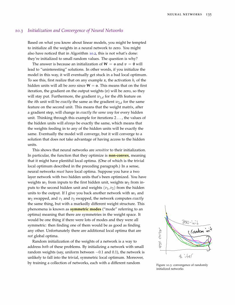
Figure 10.3: convergence of randomlyinitialized networks

Random initialization of the weights of a network is a way toaddress both of these problems. By initializing a network with smallrandom weights (say, uniform between −0.1 and 0.1), the network isunlikely to fall into the trivial, symmetric local optimum. Moreover,by training a collection of networks, each with a different random

136 a course in machine learning

initialization, you can often obtain better solutions that with justone initialization. In other words, you can train ten networks withdifferent random seeds, and then pick the one that does best on held-out data. Figure 10.3 shows prototypical test-set performance for tennetworks with different random initialization, plus an eleventh plotfor the trivial symmetric network initialized with zeros.

One of the typical complaints about neural networks is that theyare finicky. In particular, they have a rather large number of knobs totune:

1. The number of layers

2. The number of hidden units per layer

3. The gradient descent learning rate η

4. The initialization

5. The stopping iteration or weight regularization

The last of these is minor (early stopping is an easy regularizationmethod that does not require much effort to tune), but the othersare somewhat significant. Even for two layer networks, having tochoose the number of hidden units, and then get the learning rateand initialization “right” can take a bit of work. Clearly it can beautomated, but nonetheless it takes time.

Another difficulty of neural networks is that their weights canbe difficult to interpret. You’ve seen that, for linear networks, youcan often interpret high weights as indicative of positive examplesand low weights as indicative of negative examples. In multilayernetworks, it becomes very difficult to try to understand what thedifferent hidden units are doing.

10.4 Beyond Two Layers

Figure 10.4: multi-layer network

The definition of neural networks and the back-propagation algo-rithm can be generalized beyond two layers to any arbitrary directedacyclic graph. In practice, it is most common to use a layered net-work like that shown in Figure 10.4 unless one has a very strongreason (aka inductive bias) to do something different. However, theview as a directed graph sheds a different sort of insight on the back-propagation algorithm.

Figure 10.5: DAG network

Suppose that your network structure is stored in some directedacyclic graph, like that in Figure 10.5. We index nodes in this graphas u, v. The activation before applying non-linearity at a node is au

and after non-linearity is hu. The graph has a single sink, which isthe output node y with activation ay (no non-linearity is performed

neural networks 137

Algorithm 27 ForwardPropagation(x)1: for all input nodes u do2: hu ← corresponding feature of x3: end for4: for all nodes v in the network whose parent’s are computed do5: av ← ∑u∈par(v) w(u,v)hu6: hv ← tanh(av)

7: end for8: return ay

Algorithm 28 BackPropagation(x, y)1: run ForwardPropagation(x) to compute activations2: ey ← y− ay // compute overall network error3: for all nodes v in the network whose error ev is computed do4: for all u ∈ par(v) do5: gu,v ← −evhu // compute gradient of this edge6: eu ← eu + evwu,v(1− tanh2(au)) // compute the “error” of the parent node7: end for8: end for9: return all gradients ge

on the output unit). The graph has D-many inputs (i.e., nodes withno parent), whose activations hu are given by an input example. Anedge (u, v) is from a parent to a child (i.e., from an input to a hiddenunit, or from a hidden unit to the sink). Each edge has a weight wu,v.We say that par(u) is the set of parents of u.

There are two relevant algorithms: forward-propagation and back-propagation. Forward-propagation tells you how to compute theactivation of the sink y given the inputs. Back-propagation computesderivatives of the edge weights for a given input.

Figure 10.6: picture of forward prop

The key aspect of the forward-propagation algorithm is to iter-atively compute activations, going deeper and deeper in the DAG.Once the activations of all the parents of a node u have been com-puted, you can compute the activation of node u. This is spelled outin Algorithm 10.4. This is also explained pictorially in Figure 10.6.

Figure 10.7: picture of back prop

Back-propagation (see Algorithm 10.4) does the opposite: it com-putes gradients top-down in the network. The key idea is to computean error for each node in the network. The error at the output unit isthe “true error.” For any input unit, the error is the amount of gradi-ent that we see coming from our children (i.e., higher in the network).These errors are computed backwards in the network (hence thename back-propagation) along with the gradients themselves. This isalso explained pictorially in Figure 10.7.

Given the back-propagation algorithm, you can directly run gradi-ent descent, using it as a subroutine for computing the gradients.

138 a course in machine learning

10.5 Breadth versus Depth

At this point, you’ve seen how to train two-layer networks and howto train arbitrary networks. You’ve also seen a theorem that saysthat two-layer networks are universal function approximators. Thisbegs the question: if two-layer networks are so great, why do we careabout deeper networks?

To understand the answer, we can borrow some ideas from CStheory, namely the idea of circuit complexity. The goal is to showthat there are functions for which it might be a “good idea” to use adeep network. In other words, there are functions that will require ahuge number of hidden units if you force the network to be shallow,but can be done in a small number of units if you allow it to be deep.The example that we’ll use is the parity function which, ironicallyenough, is just a generalization of the XOR problem. The function isdefined over binary inputs as:

parity(x) = ∑d

xd mod 2 (10.12)

=

{1 if the number of 1s in x is odd0 if the number of 1s in x is even

(10.13)

Figure 10.8: nnet:paritydeep: deepfunction for computing parity

It is easy to define a circuit of depth O(log2 D) with O(D)-manygates for computing the parity function. Each gate is an XOR, ar-ranged in a complete binary tree, as shown in Figure 10.8. (If youwant to disallow XOR as a gate, you can fix this by allowing thedepth to be doubled and replacing each XOR with an AND, OR andNOT combination, like you did at the beginning of this chapter.)

This shows that if you are allowed to be deep, you can construct acircuit with that computes parity using a number of hidden units thatis linear in the dimensionality. So can you do the same with shallowcircuits? The answer is no. It’s a famous result of circuit complexitythat parity requires exponentially many gates to compute in constantdepth. The formal theorem is below:

Theorem 11 (Parity Function Complexity). Any circuit of depth K <

log2 D that computes the parity function of D input bits must contain OeD

gates.

This is a very famous result because it shows that constant-depthcircuits are less powerful that deep circuits. Although a neural net-work isn’t exactly the same as a circuit, the is generally believed thatthe same result holds for neural networks. At the very least, thisgives a strong indication that depth might be an important considera-tion in neural networks. What is it about neural networks

that makes it so that the theoremabout circuits does not apply di-rectly?

?One way of thinking about the issue of breadth versus depth hasto do with the number of parameters that need to be estimated. By

neural networks 139

the heuristic that you need roughly one or two examples for everyparameter, a deep model could potentially require exponentiallyfewer examples to train than a shallow model!

This now flips the question: if deep is potentially so much better,why doesn’t everyone use deep networks? There are at least twoanswers. First, it makes the architecture selection problem moresignificant. Namely, when you use a two-layer network, the onlyhyperparameter to choose is how many hidden units should go inthe middle layer. When you choose a deep network, you need tochoose how many layers, and what is the width of all those layers.This can be somewhat daunting.

A second issue has to do with training deep models with back-propagation. In general, as back-propagation works its way downthrough the model, the sizes of the gradients shrink. You can workthis out mathematically, but the intuition is simpler. If you are thebeginning of a very deep network, changing one single weight isunlikely to have a significant effect on the output, since it has togo through so many other units before getting there. This directlyimplies that the derivatives are small. This, in turn, means that back-propagation essentially never moves far from its initialization whenrun on very deep networks. While these small derivatives might

make training difficult, they mightbe good for other reasons: whatreasons?

?Finding good ways to train deep networks is an active researcharea. There are two general strategies. The first is to attempt to ini-tialize the weights better, often by a layer-wise initialization strategy.This can be often done using unlabeled data. After this initializa-tion, back-propagation can be run to tweak the weights for whateverclassification problem you care about. A second approach is to use amore complex optimization procedure, rather than gradient descent.You will learn about some such procedures later in this book.

10.6 Basis Functions

At this point, we’ve seen that: (a) neural networks can mimic linearfunctions and (b) they can learn more complex functions. A rea-sonable question is whether they can mimic a KNN classifier, andwhether they can do it efficiently (i.e., with not-too-many hiddenunits).

A natural way to train a neural network to mimic a KNN classifieris to replace the sigmoid link function with a radial basis function(RBF). In a sigmoid network (i.e., a network with sigmoid links),the hidden units were computed as hi = tanh(wi, x·). In an RBFnetwork, the hidden units are computed as:

hi = exp[−γi ||wi − x||2

](10.14)

140 a course in machine learning

Figure 10.9: nnet:rbfpicture: a one-Dpicture of RBF bumps

Figure 10.10: nnet:unitsymbols: pictureof nnet with sigmoid/rbf units

In other words, the hidden units behave like little Gaussian “bumps”centered around locations specified by the vectors wi. A one-dimensionalexample is shown in Figure 10.9. The parameter γi specifies the widthof the Gaussian bump. If γi is large, then only data points that arereally close to wi have non-zero activations. To distinguish sigmoidnetworks from RBF networks, the hidden units are typically drawnwith sigmoids or with Gaussian bumps, as in Figure 10.10.

Training RBF networks involves finding good values for the Gas-sian widths, γi, the centers of the Gaussian bumps, wi and the con-nections between the Gaussian bumps and the output unit, v. Thiscan all be done using back-propagation. The gradient terms for v re-main unchanged from before, the the derivates for the other variablesdiffer (see Exercise ??).

One of the big questions with RBF networks is: where shouldthe Gaussian bumps be centered? One can, of course, apply back-propagation to attempt to find the centers. Another option is to spec-ify them ahead of time. For instance, one potential approach is tohave one RBF unit per data point, centered on that data point. If youcarefully choose the γs and vs, you can obtain something that looksnearly identical to distance-weighted KNN by doing so. This has theadded advantage that you can go futher, and use back-propagationto learn good Gaussian widths (γ) and “voting” factors (v) for thenearest neighbor algorithm.

Consider an RBF network withone hidden unit per training point,centered at that point. What badthing might happen if you use back-propagation to estimate the γs andv on this data if you’re not careful?How could you be careful?

?

10.7 Further Reading

TODO further reading