4 | THE PERCEPTRON

Dependencies: Chapter 1, Chapter 3

So far, you’ve seen two types of learning models: in decisiontrees, only a small number of features are used to make decisions; innearest neighbor algorithms, all features are used equally. Neither ofthese extremes is always desirable. In some problems, we might wantto use most of the features, but use some more than others.

In this chapter, we’ll discuss the perceptron algorithm for learn-ing weights for features. As we’ll see, learning weights for featuresamounts to learning a hyperplane classifier: that is, basically a di-vision of space into two halves by a straight line, where one half is“positive” and one half is “negative.” In this sense, the perceptroncan be seen as explicitly finding a good linear decision boundary.

4.1 Bio-inspired Learning

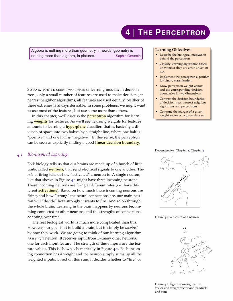
Figure 4.1: a picture of a neuron

Folk biology tells us that our brains are made up of a bunch of littleunits, called neurons, that send electrical signals to one another. Therate of firing tells us how “activated” a neuron is. A single neuron,like that shown in Figure 4.1 might have three incoming neurons.These incoming neurons are firing at different rates (i.e., have dif-ferent activations). Based on how much these incoming neurons arefiring, and how “strong” the neural connections are, our main neu-ron will “decide” how strongly it wants to fire. And so on throughthe whole brain. Learning in the brain happens by neurons becom-ming connected to other neurons, and the strengths of connectionsadapting over time.

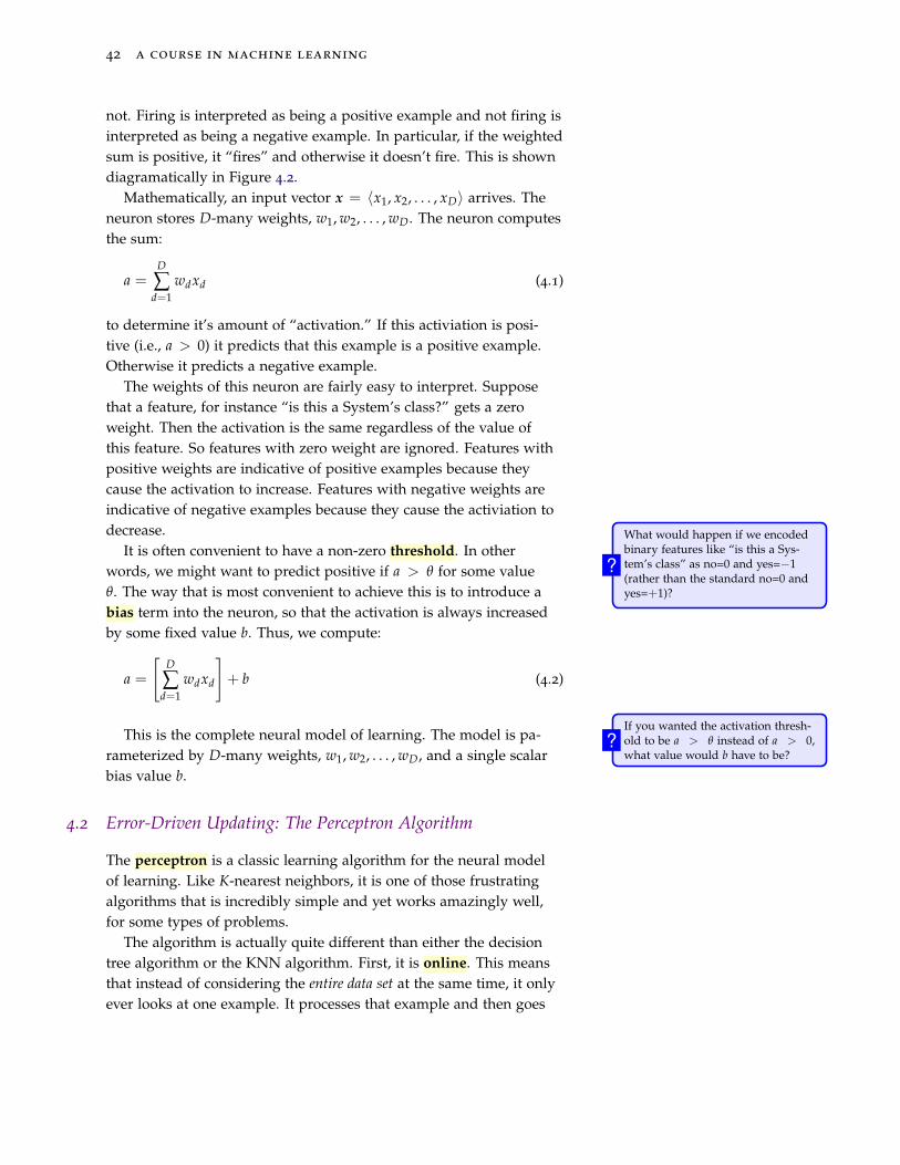
Figure 4.2: figure showing featurevector and weight vector and productsand sum

The real biological world is much more complicated than this.However, our goal isn’t to build a brain, but to simply be inspiredby how they work. We are going to think of our learning algorithmas a single neuron. It receives input from D-many other neurons,one for each input feature. The strength of these inputs are the fea-ture values. This is shown schematically in Figure 4.1. Each incom-ing connection has a weight and the neuron simply sums up all theweighted inputs. Based on this sum, it decides whether to “fire” or

Learning Objectives:• Describe the biological motivation

behind the perceptron.

• Classify learning algorithms basedon whether they are error-driven ornot.

• Implement the perceptron algorithmfor binary classification.

• Draw perceptron weight vectorsand the corresponding decisionboundaries in two dimensions.

• Contrast the decision boundariesof decision trees, nearest neighboralgorithms and perceptrons.

• Compute the margin of a givenweight vector on a given data set.

Algebra is nothing more than geometry, in words; geometry isnothing more than algebra, in pictures. – Sophie Germain

42 a course in machine learning

not. Firing is interpreted as being a positive example and not firing isinterpreted as being a negative example. In particular, if the weightedsum is positive, it “fires” and otherwise it doesn’t fire. This is showndiagramatically in Figure 4.2.

Mathematically, an input vector x = 〈x1, x2, . . . , xD〉 arrives. Theneuron stores D-many weights, w1, w2, . . . , wD. The neuron computesthe sum:

a =D

∑d=1

wdxd (4.1)

to determine it’s amount of “activation.” If this activiation is posi-tive (i.e., a > 0) it predicts that this example is a positive example.Otherwise it predicts a negative example.

The weights of this neuron are fairly easy to interpret. Supposethat a feature, for instance “is this a System’s class?” gets a zeroweight. Then the activation is the same regardless of the value ofthis feature. So features with zero weight are ignored. Features withpositive weights are indicative of positive examples because theycause the activation to increase. Features with negative weights areindicative of negative examples because they cause the activiation todecrease. What would happen if we encoded

binary features like “is this a Sys-tem’s class” as no=0 and yes=−1(rather than the standard no=0 andyes=+1)?

?It is often convenient to have a non-zero threshold. In other

words, we might want to predict positive if a > θ for some valueθ. The way that is most convenient to achieve this is to introduce abias term into the neuron, so that the activation is always increasedby some fixed value b. Thus, we compute:

a =

[D

∑d=1

wdxd

]+ b (4.2)

If you wanted the activation thresh-old to be a > θ instead of a > 0,what value would b have to be?

?This is the complete neural model of learning. The model is pa-rameterized by D-many weights, w1, w2, . . . , wD, and a single scalarbias value b.

4.2 Error-Driven Updating: The Perceptron Algorithm

The perceptron is a classic learning algorithm for the neural modelof learning. Like K-nearest neighbors, it is one of those frustratingalgorithms that is incredibly simple and yet works amazingly well,for some types of problems.

The algorithm is actually quite different than either the decisiontree algorithm or the KNN algorithm. First, it is online. This meansthat instead of considering the entire data set at the same time, it onlyever looks at one example. It processes that example and then goes

the perceptron 43

Algorithm 5 PerceptronTrain(D, MaxIter)1: wd ← 0, for all d = 1 . . . D // initialize weights2: b ← 0 // initialize bias3: for iter = 1 . . . MaxIter do4: for all (x,y) ∈ D do5: a ← ∑D

d=1 wd xd + b // compute activation for this example6: if ya ≤ 0 then7: wd ← wd + yxd, for all d = 1 . . . D // update weights8: b ← b + y // update bias9: end if

10: end for11: end for12: return w0, w1, . . . , wD, b

Algorithm 6 PerceptronTest(w0, w1, . . . , wD, b, x)1: a ← ∑D

d=1 wd xd + b // compute activation for the test example2: return sign(a)

on to the next one. Second, it is error driven. This means that, solong as it is doing well, it doesn’t bother updating its parameters.

The algorithm maintains a “guess” at good parameters (weightsand bias) as it runs. It processes one example at a time. For a givenexample, it makes a prediction. It checks to see if this predictionis correct (recall that this is training data, so we have access to truelabels). If the prediction is correct, it does nothing. Only when theprediction is incorrect does it change its parameters, and it changesthem in such a way that it would do better on this example nexttime around. It then goes on to the next example. Once it hits thelast example in the training set, it loops back around for a specifiednumber of iterations.

The training algorithm for the perceptron is shown in Algo-rithm 4.2 and the corresponding prediction algorithm is shown inAlgorithm 4.2. There is one “trick” in the training algorithm, whichprobably seems silly, but will be useful later. It is in line 6, when wecheck to see if we want to make an update or not. We want to makean update if the current prediction (just sign(a)) is incorrect. Thetrick is to multiply the true label y by the activation a and comparethis against zero. Since the label y is either +1 or −1, you just needto realize that ya is positive whenever a and y have the same sign.In other words, the product ya is positive if the current prediction iscorrect. It is very very important to check

ya ≤ 0 rather than ya < 0. Why??The particular form of update for the perceptron is quite simple.The weight wd is increased by yxd and the bias is increased by y. Thegoal of the update is to adjust the parameters so that they are “bet-ter” for the current example. In other words, if we saw this example

44 a course in machine learning

twice in a row, we should do a better job the second time around.To see why this particular update achieves this, consider the fol-

lowing scenario. We have some current set of parameters w1, . . . , wD, b.We observe an example (x, y). For simplicity, suppose this is a posi-tive example, so y = +1. We compute an activation a, and make anerror. Namely, a < 0. We now update our weights and bias. Let’s callthe new weights w′1, . . . , w′D, b′. Suppose we observe the same exam-ple again and need to compute a new activation a′. We proceed by alittle algebra:

a′ =D

∑d=1

w′dxd + b′ (4.3)

=D

∑d=1

(wd + xd)xd + (b + 1) (4.4)

=D

∑d=1

wdxd + b +D

∑d=1

xdxd + 1 (4.5)

= a +D

∑d=1

x2d + 1 > a (4.6)

So the difference between the old activation a and the new activa-tion a′ is ∑d x2

d + 1. But x2d ≥ 0, since it’s squared. So this value is

always at least one. Thus, the new activation is always at least the oldactivation plus one. Since this was a positive example, we have suc-cessfully moved the activation in the proper direction. (Though notethat there’s no guarantee that we will correctly classify this point thesecond, third or even fourth time around!) This analysis hold for the case pos-

itive examples (y = +1). It shouldalso hold for negative examples.Work it out.

?

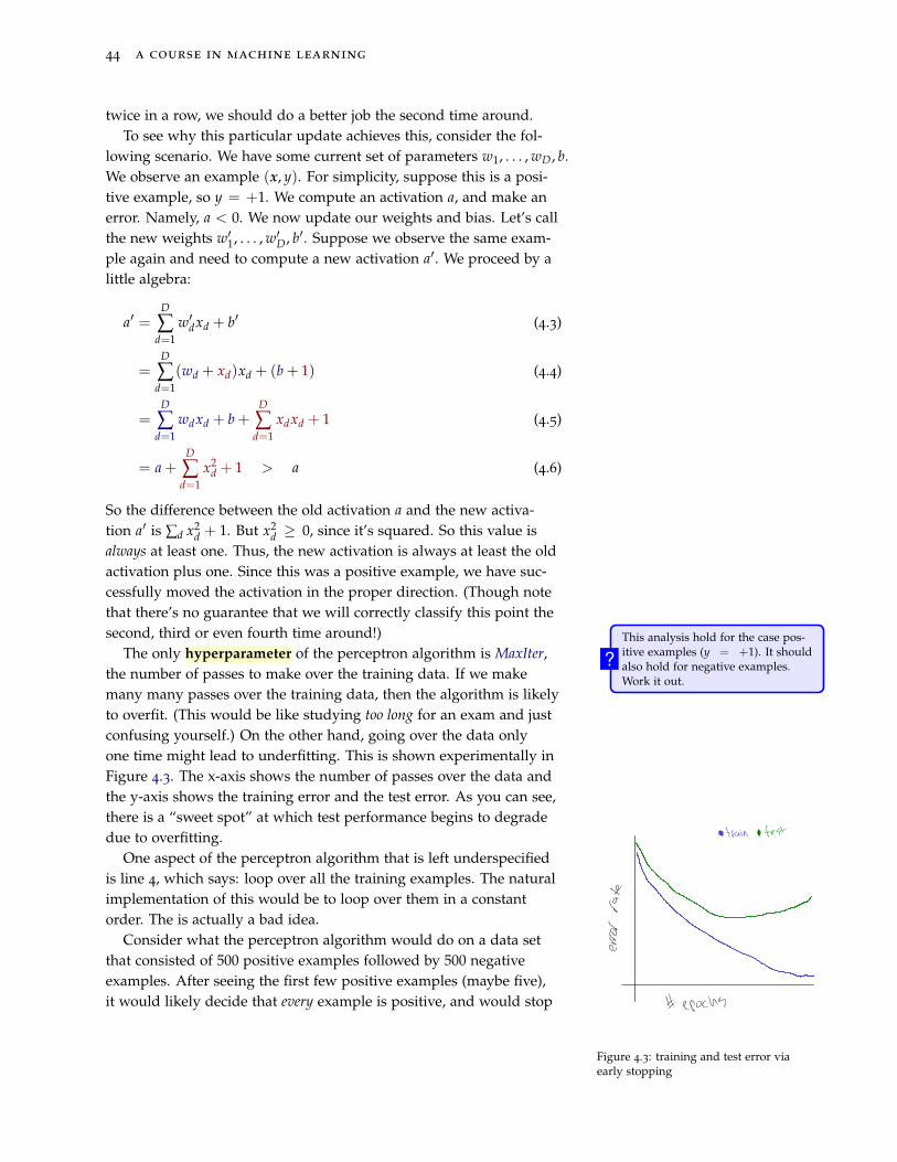
Figure 4.3: training and test error viaearly stopping

The only hyperparameter of the perceptron algorithm is MaxIter,the number of passes to make over the training data. If we makemany many passes over the training data, then the algorithm is likelyto overfit. (This would be like studying too long for an exam and justconfusing yourself.) On the other hand, going over the data onlyone time might lead to underfitting. This is shown experimentally inFigure 4.3. The x-axis shows the number of passes over the data andthe y-axis shows the training error and the test error. As you can see,there is a “sweet spot” at which test performance begins to degradedue to overfitting.

One aspect of the perceptron algorithm that is left underspecifiedis line 4, which says: loop over all the training examples. The naturalimplementation of this would be to loop over them in a constantorder. The is actually a bad idea.

Consider what the perceptron algorithm would do on a data setthat consisted of 500 positive examples followed by 500 negativeexamples. After seeing the first few positive examples (maybe five),it would likely decide that every example is positive, and would stop

the perceptron 45

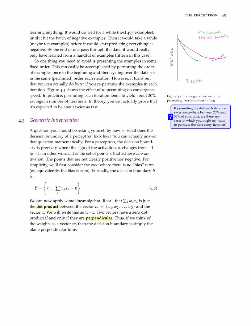
learning anything. It would do well for a while (next 495 examples),until it hit the batch of negative examples. Then it would take a while(maybe ten examples) before it would start predicting everything asnegative. By the end of one pass through the data, it would reallyonly have learned from a handful of examples (fifteen in this case).

Figure 4.4: training and test error forpermuting versus not-permuting

So one thing you need to avoid is presenting the examples in somefixed order. This can easily be accomplished by permuting the orderof examples once in the beginning and then cycling over the data setin the same (permuted) order each iteration. However, it turns outthat you can actually do better if you re-permute the examples in eachiteration. Figure 4.4 shows the effect of re-permuting on convergencespeed. In practice, permuting each iteration tends to yield about 20%savings in number of iterations. In theory, you can actually prove thatit’s expected to be about twice as fast. If permuting the data each iteration

saves somewhere between 20% and50% of your time, are there anycases in which you might not wantto permute the data every iteration?

?4.3 Geometric Intrepretation

A question you should be asking yourself by now is: what does thedecision boundary of a perceptron look like? You can actually answerthat question mathematically. For a perceptron, the decision bound-ary is precisely where the sign of the activation, a, changes from −1to +1. In other words, it is the set of points x that achieve zero ac-tivation. The points that are not clearly positive nor negative. Forsimplicity, we’ll first consider the case where there is no “bias” term(or, equivalently, the bias is zero). Formally, the decision boundary Bis:

B =

{x : ∑

dwdxd = 0

}(4.7)

We can now apply some linear algebra. Recall that ∑d wdxd is justthe dot product between the vector w = 〈w1, w2, . . . , wD〉 and thevector x. We will write this as w · x. Two vectors have a zero dotproduct if and only if they are perpendicular. Thus, if we think ofthe weights as a vector w, then the decision boundary is simply theplane perpendicular to w.

46 a course in machine learning

u

v }a} b

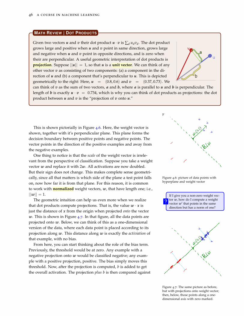
Given two vectors u and v their dot product u · v is ∑d udvd. The dot productgrows large and positive when u and v point in same direction, grows largeand negative when u and v point in opposite directions, and is zero whentheir are perpendicular. A useful geometric interpretation of dot products isprojection. Suppose ||u|| = 1, so that u is a unit vector. We can think of anyother vector v as consisting of two components: (a) a component in the di-rection of u and (b) a component that’s perpendicular to u. This is depictedgeometrically to the right: Here, u = 〈0.8, 0.6〉 and v = 〈0.37, 0.73〉. Wecan think of v as the sum of two vectors, a and b, where a is parallel to u and b is perpendicular. Thelength of b is exactly u · v = 0.734, which is why you can think of dot products as projections: the dotproduct between u and v is the “projection of v onto u.”

MATH REVIEW | DOT PRODUCTS

Figure 4.5:

Figure 4.6: picture of data points withhyperplane and weight vector

This is shown pictorially in Figure 4.6. Here, the weight vector isshown, together with it’s perpendicular plane. This plane forms thedecision boundary between positive points and negative points. Thevector points in the direction of the positive examples and away fromthe negative examples.

One thing to notice is that the scale of the weight vector is irrele-vant from the perspective of classification. Suppose you take a weightvector w and replace it with 2w. All activations are now doubled.But their sign does not change. This makes complete sense geometri-cally, since all that matters is which side of the plane a test point fallson, now how far it is from that plane. For this reason, it is commonto work with normalized weight vectors, w, that have length one; i.e.,||w|| = 1. If I give you a non-zero weight vec-

tor w, how do I compute a weightvector w′ that points in the samedirection but has a norm of one?

?

Figure 4.7: The same picture as before,but with projections onto weight vector;then, below, those points along a one-dimensional axis with zero marked.

The geometric intuition can help us even more when we realizethat dot products compute projections. That is, the value w · x isjust the distance of x from the origin when projected onto the vectorw. This is shown in Figure 4.7. In that figure, all the data points areprojected onto w. Below, we can think of this as a one-dimensionalversion of the data, where each data point is placed according to itsprojection along w. This distance along w is exactly the activiation ofthat example, with no bias.

From here, you can start thinking about the role of the bias term.Previously, the threshold would be at zero. Any example with anegative projection onto w would be classified negative; any exam-ple with a positive projection, positive. The bias simply moves thisthreshold. Now, after the projection is computed, b is added to getthe overall activation. The projection plus b is then compared against

the perceptron 47

zero.

Figure 4.8: perc:bias: perceptronpicture with bias

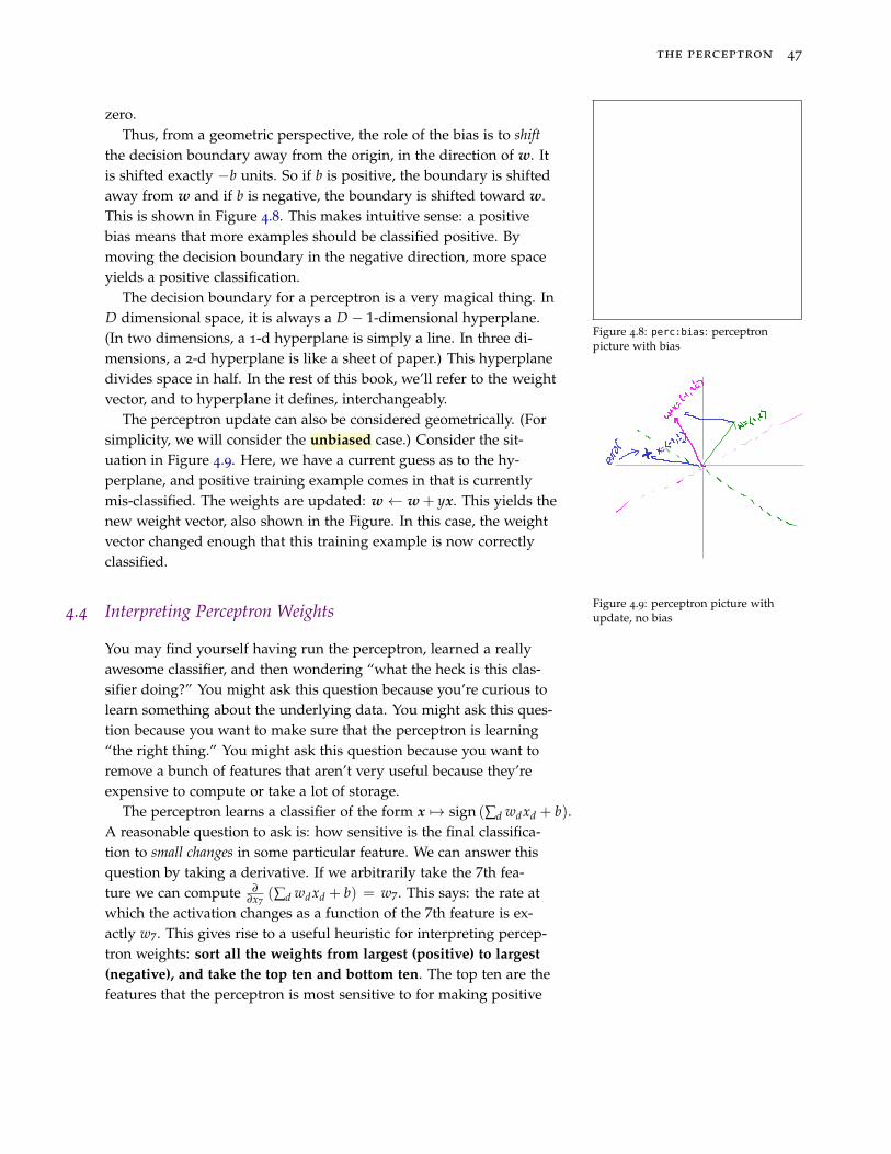
Thus, from a geometric perspective, the role of the bias is to shiftthe decision boundary away from the origin, in the direction of w. Itis shifted exactly −b units. So if b is positive, the boundary is shiftedaway from w and if b is negative, the boundary is shifted toward w.This is shown in Figure 4.8. This makes intuitive sense: a positivebias means that more examples should be classified positive. Bymoving the decision boundary in the negative direction, more spaceyields a positive classification.

The decision boundary for a perceptron is a very magical thing. InD dimensional space, it is always a D − 1-dimensional hyperplane.(In two dimensions, a 1-d hyperplane is simply a line. In three di-mensions, a 2-d hyperplane is like a sheet of paper.) This hyperplanedivides space in half. In the rest of this book, we’ll refer to the weightvector, and to hyperplane it defines, interchangeably.

Figure 4.9: perceptron picture withupdate, no bias

The perceptron update can also be considered geometrically. (Forsimplicity, we will consider the unbiased case.) Consider the sit-uation in Figure 4.9. Here, we have a current guess as to the hy-perplane, and positive training example comes in that is currentlymis-classified. The weights are updated: w← w + yx. This yields thenew weight vector, also shown in the Figure. In this case, the weightvector changed enough that this training example is now correctlyclassified.

4.4 Interpreting Perceptron Weights

You may find yourself having run the perceptron, learned a reallyawesome classifier, and then wondering “what the heck is this clas-sifier doing?” You might ask this question because you’re curious tolearn something about the underlying data. You might ask this ques-tion because you want to make sure that the perceptron is learning“the right thing.” You might ask this question because you want toremove a bunch of features that aren’t very useful because they’reexpensive to compute or take a lot of storage.

The perceptron learns a classifier of the form x 7→ sign (∑d wdxd + b).A reasonable question to ask is: how sensitive is the final classifica-tion to small changes in some particular feature. We can answer thisquestion by taking a derivative. If we arbitrarily take the 7th fea-ture we can compute ∂

∂x7(∑d wdxd + b) = w7. This says: the rate at

which the activation changes as a function of the 7th feature is ex-actly w7. This gives rise to a useful heuristic for interpreting percep-tron weights: sort all the weights from largest (positive) to largest(negative), and take the top ten and bottom ten. The top ten are thefeatures that the perceptron is most sensitive to for making positive

48 a course in machine learning

predictions. The bottom ten are the features that the perceptron ismost sensitive to for making negative predictions.

This heuristic is useful, especially when the inputs x consist en-tirely of binary values (like a bag of words representation). Theheuristic is less useful when the range of the individual featuresvaries significantly. The issue is that if you have one feat x5 that’s ei-ther 0 or 1, and another feature x7 that’s either 0 or 100, but w5 = w7,it’s reasonable to say that w7 is more important because it is likely tohave a much larger influence on the final prediction. The easiest wayto compensate for this is simply to scale your features ahead of time:this is another reason why feature scaling is a useful preprocessingstep.

4.5 Perceptron Convergence and Linear Separability

You already have an intuitive feeling for why the perceptron works:it moves the decision boundary in the direction of the training exam-ples. A question you should be asking yourself is: does the percep-tron converge? If so, what does it converge to? And how long does ittake?

It is easy to construct data sets on which the perceptron algorithmwill never converge. In fact, consider the (very uninteresting) learn-ing problem with no features. You have a data set consisting of onepositive example and one negative example. Since there are no fea-tures, the only thing the perceptron algorithm will ever do is adjustthe bias. Given this data, you can run the perceptron for a bajillioniterations and it will never settle down. As long as the bias is non-negative, the negative example will cause it to decrease. As long asit is non-positive, the positive example will cause it to increase. Adinfinitum. (Yes, this is a very contrived example.)

Figure 4.10: separable data

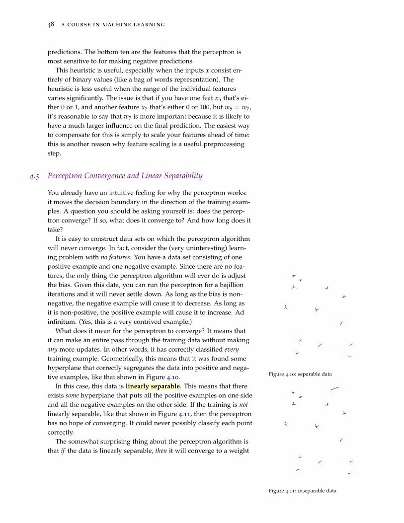
What does it mean for the perceptron to converge? It means thatit can make an entire pass through the training data without makingany more updates. In other words, it has correctly classified everytraining example. Geometrically, this means that it was found somehyperplane that correctly segregates the data into positive and nega-tive examples, like that shown in Figure 4.10.

Figure 4.11: inseparable data

In this case, this data is linearly separable. This means that thereexists some hyperplane that puts all the positive examples on one sideand all the negative examples on the other side. If the training is notlinearly separable, like that shown in Figure 4.11, then the perceptronhas no hope of converging. It could never possibly classify each pointcorrectly.

The somewhat surprising thing about the perceptron algorithm isthat if the data is linearly separable, then it will converge to a weight

the perceptron 49

vector that separates the data. (And if the data is inseparable, then itwill never converge.) This is great news. It means that the perceptronconverges whenever it is even remotely possible to converge.

The second question is: how long does it take to converge? By“how long,” what we really mean is “how many updates?” As is thecase for much learning theory, you will not be able to get an answerof the form “it will converge after 5293 updates.” This is asking toomuch. The sort of answer we can hope to get is of the form “it willconverge after at most 5293 updates.”

What you might expect to see is that the perceptron will con-verge more quickly for easy learning problems than for hard learningproblems. This certainly fits intuition. The question is how to define“easy” and “hard” in a meaningful way. One way to make this def-inition is through the notion of margin. If I give you a data set andhyperplane that separates itthen the margin is the distance betweenthe hyperplane and the nearest point. Intuitively, problems with largemargins should be easy (there’s lots of “wiggle room” to find a sepa-rating hyperplane); and problems with small margins should be hard(you really have to get a very specific well tuned weight vector).

Formally, given a data set D, a weight vector w and bias b, themargin of w, b on D is defined as:

margin(D, w, b) =

{min(x,y)∈D y

(w · x + b

)if w separates D

−∞ otherwise(4.8)

In words, the margin is only defined if w, b actually separate the data(otherwise it is just −∞). In the case that it separates the data, wefind the point with the minimum activation, after the activation ismultiplied by the label. So long as the margin is not −∞,

it is always positive. Geometricallythis makes sense, but why doesEq (4.8) yield this?

?For some historical reason (that is unknown to the author), mar-gins are always denoted by the Greek letter γ (gamma). One oftentalks about the margin of a data set. The margin of a data set is thelargest attainable margin on this data. Formally:

margin(D) = supw,b

margin(D, w, b) (4.9)

In words, to compute the margin of a data set, you “try” every possi-ble w, b pair. For each pair, you compute its margin. We then take thelargest of these as the overall margin of the data.1 If the data is not 1 You can read “sup” as “max” if you

like: the only difference is a technicaldifference in how the −∞ case ishandled.

linearly separable, then the value of the sup, and therefore the valueof the margin, is −∞.

There is a famous theorem due to Rosenblatt2 that shows that the 2 Rosenblatt 1958

number of errors that the perceptron algorithm makes is bounded byγ−2. More formally:

50 a course in machine learning

Theorem 2 (Perceptron Convergence Theorem). Suppose the perceptronalgorithm is run on a linearly separable data set D with margin γ > 0.Assume that ||x|| ≤ 1 for all x ∈ D. Then the algorithm will converge afterat most 1

γ2 updates.

The proof of this theorem is elementary, in the sense that it doesnot use any fancy tricks: it’s all just algebra. The idea behind theproof is as follows. If the data is linearly separable with margin γ,then there exists some weight vector w∗ that achieves this margin.Obviously we don’t know what w∗ is, but we know it exists. Theperceptron algorithm is trying to find a weight vector w that pointsroughly in the same direction as w∗. (For large γ, “roughly” can bevery rough. For small γ, “roughly” is quite precise.) Every time theperceptron makes an update, the angle between w and w∗ changes.What we prove is that the angle actually decreases. We show this intwo steps. First, the dot product w ·w∗ increases a lot. Second, thenorm ||w|| does not increase very much. Since the dot product isincreasing, but w isn’t getting too long, the angle between them hasto be shrinking. The rest is algebra.

Proof of Theorem 2. The margin γ > 0 must be realized by some setof parameters, say x∗. Suppose we train a perceptron on this data.Denote by w(0) the initial weight vector, w(1) the weight vector afterthe first update, and w(k) the weight vector after the kth update. (Weare essentially ignoring data points on which the perceptron doesn’tupdate itself.) First, we will show that w∗ · w(k) grows quicky asa function of k. Second, we will show that

∣∣∣∣w(k)∣∣∣∣ does not grow

quickly.First, suppose that the kth update happens on example (x, y). We

are trying to show that w(k) is becoming aligned with w∗. Because weupdated, know that this example was misclassified: yw(k-1) · x < 0.After the update, we get w(k) = w(k-1) + yx. We do a little computa-tion:

w∗ ·w(k) = w∗ ·(

w(k-1) + yx)

definition of w(k) (4.10)

= w∗ ·w(k-1) + yw∗ · x vector algebra (4.11)

≥ w∗ ·w(k-1) + γ w∗ has margin γ (4.12)

Thus, every time w(k) is updated, its projection onto w∗ increases byat least γ. Therefore: w∗ ·w(k) ≥ kγ.

Next, we need to show that the increase of γ along w∗ occursbecause w(k) is getting closer to w∗, not just because it’s getting ex-ceptionally long. To do this, we compute the norm of w(k):∣∣∣∣∣∣w(k)

∣∣∣∣∣∣2

the perceptron 51

=∣∣∣∣∣∣w(k-1) + yx

∣∣∣∣∣∣2 def. of w(k) (4.13)

=∣∣∣∣∣∣w(k-1)

∣∣∣∣∣∣2 + y2 ||x||2 + 2yw(k-1) · x quadratic rule (4.14)

≤∣∣∣∣∣∣w(k-1)

∣∣∣∣∣∣2 + 1 + 0 assumption and a < 0 (4.15)

Thus, the squared norm of w(k) increases by at most one every up-date. Therefore:

∣∣∣∣w(k)∣∣∣∣2 ≤ k.

Now we put together the two things we have learned before. Byour first conclusion, we know w∗ ·w(k) ≥ kγ. But our second con-clusion,

√k ≥

∣∣∣∣w(k)∣∣∣∣2. Finally, because w∗ is a unit vector, we know

that∣∣∣∣w(k)

∣∣∣∣ ≥ w∗ ·w(k). Putting this together, we have:

√k ≥

∣∣∣∣∣∣w(k)∣∣∣∣∣∣ ≥ w∗ ·w(k) ≥ kγ (4.16)

Taking the left-most and right-most terms, we get that√

k ≥ kγ.Dividing both sides by k, we get 1√

k≥ γ and therefore k ≤ 1

γ2 .

This means that once we’ve made 1γ2 updates, we cannot make any

more!

Perhaps we don’t want to assumethat all x have norm at most 1. Ifthey have all have norm at mostR, you can achieve a very simi-lar bound. Modify the perceptronconvergence proof to handle thiscase.

?

It is important to keep in mind what this proof shows and whatit does not show. It shows that if I give the perceptron data thatis linearly separable with margin γ > 0, then the perceptron willconverge to a solution that separates the data. And it will convergequickly when γ is large. It does not say anything about the solution,other than the fact that it separates the data. In particular, the proofmakes use of the maximum margin separator. But the perceptronis not guaranteed to find this maximum margin separator. The datamay be separable with margin 0.9 and the perceptron might stillfind a separating hyperplane with a margin of only 0.000001. Later(in Chapter 8), we will see algorithms that explicitly try to find themaximum margin solution. Why does the perceptron conver-

gence bound not contradict theearlier claim that poorly ordereddata points (e.g., all positives fol-lowed by all negatives) will causethe perceptron to take an astronom-ically long time to learn?

?4.6 Improved Generalization: Voting and Averaging

In the beginning of this chapter, there was a comment that the per-ceptron works amazingly well. This was a half-truth. The “vanilla”perceptron algorithm does well, but not amazingly well. In order tomake it more competitive with other learning algorithms, you needto modify it a bit to get better generalization. The key issue with thevanilla perceptron is that it counts later points more than it counts earlierpoints.

To see why, consider a data set with 10, 000 examples. Supposethat after the first 100 examples, the perceptron has learned a really

52 a course in machine learning

good classifier. It’s so good that it goes over the next 9899 exam-ples without making any updates. It reaches the 10, 000th exampleand makes an error. It updates. For all we know, the update on this10, 000th example completely ruins the weight vector that has done sowell on 99.99% of the data!

What we would like is for weight vectors that “survive” a longtime to get more say than weight vectors that are overthrown quickly.One way to achieve this is by voting. As the perceptron learns, itremembers how long each hyperplane survives. At test time, eachhyperplane encountered during training “votes” on the class of a testexample. If a particular hyperplane survived for 20 examples, thenit gets a vote of 20. If it only survived for one example, it only gets avote of 1. In particular, let (w, b)(1), . . . , (w, b)(K) be the K + 1 weightvectors encountered during training, and c(1), . . . , c(K) be the survivaltimes for each of these weight vectors. (A weight vector that getsimmediately updated gets c = 1; one that survives another roundgets c = 2 and so on.) Then the prediction on a test point is:

y = sign

(K

∑k=1

c(k)sign(

w(k) · x + b(k)))

(4.17)

This algorithm, known as the voted perceptron works quite well inpractice, and there is some nice theory showing that it is guaranteedto generalize better than the vanilla perceptron. Unfortunately, it isalso completely impractical. If there are 1000 updates made duringperceptron learning, the voted perceptron requires that you store1000 weight vectors, together with their counts. This requires anabsurd amount of storage, and makes prediction 1000 times slowerthan the vanilla perceptron. The training algorithm for the voted

perceptron is the same as thevanilla perceptron. In particular,in line 5 of Algorithm 4.2, the ac-tivation on a training example iscomputed based on the currentweight vector, not based on the votedprediction. Why?

?

A much more practical alternative is the averaged perceptron.The idea is similar: you maintain a collection of weight vectors andsurvival times. However, at test time, you predict according to theaverage weight vector, rather than the voting. In particular, the predic-tion is:

y = sign

(K

∑k=1

c(k)(

w(k) · x + b(k)))

(4.18)

The only difference between the voted prediction, Eq (4.17), and theaveraged prediction, Eq (4.18), is the presense of the interior signoperator. With a little bit of algebra, we can rewrite the test-timeprediction as:

y = sign

((K

∑k=1

c(k)w(k)

)· x +

K

∑k=1

c(k)b(k)

)(4.19)

The advantage of the averaged perceptron is that we can simplymaintain a running sum of the averaged weight vector (the blue term)

the perceptron 53

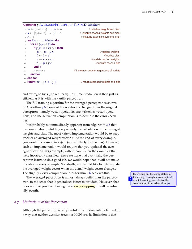
Algorithm 7 AveragedPerceptronTrain(D, MaxIter)1: w ← 〈0, 0, . . . 0〉 , b ← 0 // initialize weights and bias2: u ← 〈0, 0, . . . 0〉 , β ← 0 // initialize cached weights and bias3: c← 1 // initialize example counter to one4: for iter = 1 . . . MaxIter do5: for all (x,y) ∈ D do6: if y(w · x + b) ≤ 0 then7: w ← w + y x // update weights8: b ← b + y // update bias9: u ← u + y c x // update cached weights

10: β ← β + y c // update cached bias11: end if12: c← c + 1 // increment counter regardless of update13: end for14: end for15: return w - 1

c u, b - 1c β // return averaged weights and bias

and averaged bias (the red term). Test-time prediction is then just asefficient as it is with the vanilla perceptron.

The full training algorithm for the averaged perceptron is shownin Algorithm 4.6. Some of the notation is changed from the originalperceptron: namely, vector operations are written as vector opera-tions, and the activation computation is folded into the error check-ing.

It is probably not immediately apparent from Algorithm 4.6 thatthe computation unfolding is precisely the calculation of the averagedweights and bias. The most natural implementation would be to keeptrack of an averaged weight vector u. At the end of every example,you would increase u ← u + w (and similarly for the bias). However,such an implementation would require that you updated the aver-aged vector on every example, rather than just on the examples thatwere incorrectly classified! Since we hope that eventually the per-ceptron learns to do a good job, we would hope that it will not makeupdates on every example. So, ideally, you would like to only updatethe averaged weight vector when the actual weight vector changes.The slightly clever computation in Algorithm 4.6 achieves this. By writing out the computation of

the averaged weights from Eq (4.18)as a telescoping sum, derive thecomputation from Algorithm 4.6.

?The averaged perceptron is almost always better than the percep-tron, in the sense that it generalizes better to test data. However, thatdoes not free you from having to do early stopping. It will, eventu-ally, overfit.

4.7 Limitations of the Perceptron

Although the perceptron is very useful, it is fundamentally limited ina way that neither decision trees nor KNN are. Its limitation is that

54 a course in machine learning

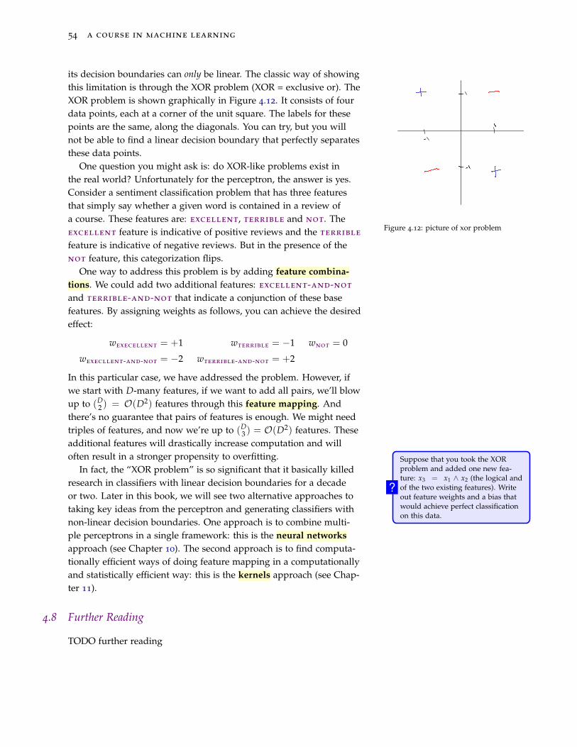
its decision boundaries can only be linear. The classic way of showingthis limitation is through the XOR problem (XOR = exclusive or). TheXOR problem is shown graphically in Figure 4.12. It consists of fourdata points, each at a corner of the unit square. The labels for thesepoints are the same, along the diagonals. You can try, but you willnot be able to find a linear decision boundary that perfectly separatesthese data points.

Figure 4.12: picture of xor problem

One question you might ask is: do XOR-like problems exist inthe real world? Unfortunately for the perceptron, the answer is yes.Consider a sentiment classification problem that has three featuresthat simply say whether a given word is contained in a review ofa course. These features are: excellent, terrible and not. Theexcellent feature is indicative of positive reviews and the terrible

feature is indicative of negative reviews. But in the presence of thenot feature, this categorization flips.

One way to address this problem is by adding feature combina-tions. We could add two additional features: excellent-and-not

and terrible-and-not that indicate a conjunction of these basefeatures. By assigning weights as follows, you can achieve the desiredeffect:

wexecellent = +1 wterrible = −1 wnot = 0

wexecllent-and-not = −2 wterrible-and-not = +2

In this particular case, we have addressed the problem. However, ifwe start with D-many features, if we want to add all pairs, we’ll blowup to (D

2 ) = O(D2) features through this feature mapping. Andthere’s no guarantee that pairs of features is enough. We might needtriples of features, and now we’re up to (D

3 ) = O(D2) features. Theseadditional features will drastically increase computation and willoften result in a stronger propensity to overfitting. Suppose that you took the XOR

problem and added one new fea-ture: x3 = x1 ∧ x2 (the logical andof the two existing features). Writeout feature weights and a bias thatwould achieve perfect classificationon this data.

?

In fact, the “XOR problem” is so significant that it basically killedresearch in classifiers with linear decision boundaries for a decadeor two. Later in this book, we will see two alternative approaches totaking key ideas from the perceptron and generating classifiers withnon-linear decision boundaries. One approach is to combine multi-ple perceptrons in a single framework: this is the neural networksapproach (see Chapter 10). The second approach is to find computa-tionally efficient ways of doing feature mapping in a computationallyand statistically efficient way: this is the kernels approach (see Chap-ter 11).

4.8 Further Reading

TODO further reading