wsrc-sti-2007-00061, rev. 2, 'life estimation of hlw tank ... · life estimation of high level...

WSRC-STI-2007-00061, Rev. 2

Life Estimation of High Level Waste Tank Steel for F-Tank Farm Closure Performance Assessment, Rev.2

K. H. Subramanian

Savannah River National Laboratory Materials Science and Technology Directorate

Publication Date: June 2008

Washington Savannah River Company Savannah River Site Aiken SC 29808

This document was prepared in connection with work done under Contract No. DE-AC09-96SR18500 with the U. S. Department of Energy

WSRC-STI-2007-00061, Rev. 2

ii

DISCLAIMER

This report was prepared as an account of work sponsored by an agency of the United States Government. Neither the United States Government nor any agency thereof, nor any of their employees, makes any warranty, express or implied, or assumes any legal liability or responsibility for the accuracy, completeness, or usefulness of any information, apparatus, product, or process disclosed, or represents that its use would not infringe privately owned rights. Reference herein to any specific commercial product, process, or service by trade name, trademark, manufacturer, or otherwise does not necessarily constitute or imply its endorsement, recommendation, or favoring by the United States Government or any agency thereof. The views and opinions of authors expressed herein do not necessarily state or reflect those of the United States Government or any agency thereof.

WSRC-STI-2007-00061, Rev. 2

iii

DOCUMENT: WSRC-STI-2007-00061, Rev. 2

TITLE: Life Estimation of High Level Waste Tank Steel for F-Tank Farm Closure Performance Assessment

APPROVALS

WSRC-STI-2007-00061, Rev. 2

iv

Table of Contents

1 SUMMARY ........................................................................................................................................................8 2 INTRODUCTION AND BACKGROUND....................................................................................................11

2.1 F-TANK FARM TANK DESIGN AND CONSTRUCTION ..................................................................................11 2.1.1 Type I Tanks.........................................................................................................................................11 2.1.2 Type III and Type IIIA Tanks ...............................................................................................................12 2.1.3 Type IV Tanks ......................................................................................................................................13

2.2 CURRENT CONDITION OF F-TANK FARM TANKS .......................................................................................13 2.2.1 Service-Induced Corrosion Mechanisms .............................................................................................14 2.2.2 Compilation of F-Tank Farm Condition..............................................................................................14 2.2.3 Stress Corrosion Crack Opening Area ................................................................................................16

3 TANK STEEL LIFE ESTIMATION TECHNICAL APPROACH.............................................................19 3.1 TANK EXPOSURES .....................................................................................................................................19 3.2 CORROSION MECHANISM IN CONTAMINATION ZONE ................................................................................21 3.3 CORROSION MECHANISMS IN CONCRETE/GROUT......................................................................................22

3.3.1 Carbonation.........................................................................................................................................23 3.3.2 Chloride Induced Corrosion................................................................................................................25 3.3.3 Microcell/Macrocell Corrosion ...........................................................................................................28 3.3.4 Microbially Induced Corrosion ...........................................................................................................29

3.4 CORROSION OF TANK STEEL EXPOSED TO SOIL ........................................................................................29 3.4.1 General Corrosion...............................................................................................................................29 3.4.2 Pitting Corrosion .................................................................................................................................30

4 TANK STEEL LIFE ESTIMATION RESULTS ..........................................................................................31 4.1 GROUTED CONDITIONS .............................................................................................................................31

4.1.1 Estimation of Type I Tank Steel Life Exposed to Grouted Conditions.................................................32 4.1.2 Estimation of Type III Tank Steel Life Exposed to Grouted Conditions ..............................................32 4.1.3 Estimation of Type IV Tank Steel Life Exposed to Grouted Conditions ..............................................33

4.2 SOIL CONDITIONS......................................................................................................................................34 4.2.1 Estimation of Type I Tank Steel Life Exposed to Soil ..........................................................................34 4.2.2 Estimation of Type III Tank Steel Life Exposed to Soil........................................................................36 4.2.3 Estimation of Type IV Tank Steel Life Exposed to Soil ........................................................................37

4.3 HUMID AIR PIPE CONDITIONS ...................................................................................................................39 5 STOCHASTIC LIFE ESTIMATION METHODOLOGY ..........................................................................42

5.1 TECHNICAL APPROACH .............................................................................................................................42 5.1.1 Initial Tank Concrete Vault Thickness.................................................................................................43 5.1.2 Tank Steel Liner Thickness ..................................................................................................................44

5.2 CORROSION INITIATION BY CHLORIDE ......................................................................................................46 5.2.1 Water to Cement Ratio Distribution ....................................................................................................46 5.2.2 Concentration of Chloride Distribution...............................................................................................46

5.3 CORROSION BY CARBONATION .................................................................................................................47 5.3.1 Inorganic Carbon Content Distribution ..............................................................................................47 5.3.2 Bulk Concentration of Ca(OH)2 Distribution (‘Cg’) ............................................................................48

5.4 CASES OF POTENTIAL CORROSION ............................................................................................................50 5.4.1 Case 1: IF tinitiation [Cl-] ≥ tinitiation [Carbonation] ................................................................................50 5.4.2 Case 2: IF tinitiation [Cl-] < tinitiation [Carbonation] .........................................................................................51 5.4.3 Case 3: IF tfailure [Cl-] ≥ tinitiation [Carbonation]............................................................................................57

6 RESULTS OF PARTIAL STOCHASTIC APPROACH .............................................................................58

WSRC-STI-2007-00061, Rev. 2

v

6.1 TYPE I TANK : DI(CO2) = 1X10-8CM2/SEC, VARIED DI (O2) ........................................................................58 6.2 TYPE I TANK : DI(CO2) = 1X10-6CM2/SEC, VARIED DI (O2) ........................................................................59 6.3 TYPE I TANK : DI(CO2) = 1X10-4CM2/SEC, VARIED DI (O2) ........................................................................60 6.4 TYPE III TANK : DI(CO2) = 1X10-8CM2/SEC, VARIED DI (O2) .....................................................................61 6.5 TYPE III TANK : DI(CO2) = 1X10-6CM2/SEC, VARIED DI (O2) .....................................................................62 6.6 TYPE III TANK : DI(CO2) = 1X10-4CM2/SEC, VARIED DI (O2) .....................................................................63 6.7 TYPE IV TANK : DI(CO2) = 1X10-8CM2/SEC, VARIED DI (O2) .....................................................................64 6.8 TYPE IV TANK : DI(CO2) = 1X10-6CM2/SEC, VARIED DI (O2) .....................................................................65 6.9 TYPE IV TANK : DI(CO2) = 1X10-4CM2/SEC, VARIED DI (O2) .....................................................................66

7 COMPREHENSIVE STOCHASTIC METHODOLOGY ...........................................................................67 7.1 CORROSION RATE DISTRIBUTION..............................................................................................................67 7.2 DISTRIBUTION OF CARBON DIOXIDE/OXYGEN DIFFUSION COEFFICIENTS.................................................69

8 RESULTS OF COMPREHENSIVE STOCHASTIC ANALYSIS ..............................................................71 9 CONCLUSION.................................................................................................................................................74 10 ACKNOWLEDGEMENTS.............................................................................................................................74 REFERENCES ..........................................................................................................................................................75

WSRC-STI-2007-00061, Rev. 2

vi

List of Tables

TABLE 1: SUMMARY OF TANK STEEL LIFE ESTIMATION RESULTS IN GROUTED CONDITIONS........................................8 TABLE 2: SUMMARY OF TANK STEEL LIFE ESTIMATION RESULTS IN SOIL CONDITIONS ................................................8 TABLE 3: LIFE ESTIMATION RESULTS FROM COMPREHENSIVE STOCHASTIC APPROACH..............................................10 TABLE 4: ASTM REQUIREMENTS FOR CHEMICAL COMPOSITION FOR A285-50T, GRADE B FIREBOX QUALITY[].......11 TABLE 5: NOMINAL COMPOSITIONS OF A516-70 AND A537-CL.1[,]............................................................................12 TABLE 6: THICKNESS OF PLATES USED IN TYPE III TANKS ..........................................................................................13 TABLE 7: CONDITION OF F-TANK FARM TANKS [5,] ....................................................................................................14 TABLE 8: CRACK OPENING AREA FOR STRESS CORROSION CRACKS............................................................................19 TABLE 9: TYPE I TANK STEEL EXPOSURE IN CLOSURE CONFIGURATION .....................................................................19 TABLE 10: TYPE III/IIIA TANK STEEL EXPOSURE IN CLOSURE CONFIGURATION.........................................................20 TABLE 11: TYPE IV TANK STEEL EXPOSURE IN CLOSURE CONDITION.........................................................................20 TABLE 12: R-VALUE OF CONTAMINATION ZONE EXPOSURE........................................................................................22 TABLE 13: INITIATION TIME FOR CHLORIDE INDUCED CORROSION..............................................................................27 TABLE 14: SOIL CONDITIONS USED FOR ANALYSIS......................................................................................................29 TABLE 15: WEIGHT LOSS OF CARBON STEEL IN CECIL CLAY LOAM SOIL....................................................................30 TABLE 16: CORROSION RATES OF VAPOR SPACE TEST COUPONS IN YUCCA MOUNTAIN STUDY .................................41 TABLE 17: TIME TO CONSUMPTION OF TANK WALL BASED UPON HUMID AIR CORROSION ........................................42 TABLE 18: DISTRIBUTIONS OF TANK CONCRETE VAULT THICKNESSES .......................................................................44 TABLE 19: DISTRIBUTION OF TANK STEEL THICKNESSES.............................................................................................45 TABLE 20: CORROSION RATES DUE TO OXALIC ACID CHEMICAL CLEANING PROCESS ................................................45 TABLE 21: FIXED VARIABLES IN CG CALCULATIONS. ...................................................................................................48 TABLE 22: UNIFORMLY DISTRIBUTED VARIABLES IN CG CALCULATIONS ....................................................................49 TABLE 23: RELATED VARIABLES IN CG CALCULATIONS...............................................................................................49 TABLE 24: CALCULATED CORROSION RATE AFTER CHLORIDE INDUCED DEPASSIVATION FOR TYPE I TANKS ............52 TABLE 25: CALCULATED CORROSION RATE AFTER CHLORIDE INDUCED DEPASSIVATION FOR TYPE III TANKS..........53 TABLE 26: CALCULATED CORROSION RATE AFTER CHLORIDE INDUCED DEPASSIVATION FOR TYPE IV TANKS..........54 TABLE 27: CORROSION RATE USED FOR SIMULATIONS AFTER CHLORIDE INDUCED DEPASSIVATION FOR TYPE I TANKS

...........................................................................................................................................................................55 TABLE 28: CORROSION RATE USED FOR SIMULATIONS AFTER CHLORIDE INDUCED DEPASSIVATION FOR TYPE III

TANKS ................................................................................................................................................................56 TABLE 29: CORROSION RATE USED FOR SIMULATIONS AFTER CHLORIDE INDUCED DEPASSIVATION FOR TYPE IV

TANKS ................................................................................................................................................................57 TABLE 30: TIME TO FAILURE FOR TYPE I TANK WHERE DI(CO2) = 1X10-8CM2/SEC, VARIED DI (O2)............................59 TABLE 31: TIME TO FAILURE FOR TYPE I TANK WHERE DI(CO2) = 1X10-6CM2/SEC, VARIED DI (O2)............................60 TABLE 32: TIME TO FAILURE FOR TYPE I TANK WHERE DI(CO2) = 1X10-4CM2/SEC, VARIED DI (O2)............................61 TABLE 33: TIME TO FAILURE FOR TYPE III TANK WHERE DI(CO2) = 1X10-8CM2/SEC, VARIED DI (O2) .........................62 TABLE 34: TIME TO FAILURE FOR TYPE III TANK WHERE DI(CO2) = 1X10-6CM2/SEC, VARIED DI (O2) .........................63 TABLE 35: TIME TO FAILURE FOR TYPE III TANK WHERE DI(CO2) = 1X10-4CM2/SEC, VARIED DI (O2) .........................64 TABLE 36: TIME TO FAILURE FOR TYPE IV TANK WHERE DI(CO2) = 1X10-8CM2/SEC, VARIED DI (O2) .........................65 TABLE 37: TIME TO FAILURE FOR TYPE IV TANK WHERE DI(CO2) = 1X10-6CM2/SEC, VARIED DI (O2) .........................66 TABLE 38: TIME TO FAILURE FOR TYPE IV TANK WHERE DI(CO2) = 1X10-4CM2/SEC, VARIED DI (O2) .........................67 TABLE 39: CORRESPONDING PASSIVE CURRENT DENSITIES FOR CORROSION RATE DISTRIBUTION.............................68 TABLE 40: TIME TO FAILURE FOR TYPE I TANK USING COMPREHENSIVE STOCHASTIC METHODOLOGY .....................71 TABLE 41: TIME TO FAILURE FOR TYPE III/IIIA TANK USING COMPREHENSIVE STOCHASTIC METHODOLOGY...........72 TABLE 42: TIME TO FAILURE FOR TYPE IV TANK USING COMPREHENSIVE STOCHASTIC METHODOLOGY ..................73

WSRC-STI-2007-00061, Rev. 2

vii

List of Figures

FIGURE 1: TYPE I TANK................................................................................................................................................11 FIGURE 2: TYPE III HIGH LEVEL WASTE TANK SCHEMATIC ........................................................................................12 FIGURE 3: TYPE IV TANK.............................................................................................................................................13 FIGURE 4: SCHEMATIC OF STRESS CORROSION CRACKING MECHANISM[] ...................................................................14 FIGURE 5: AXIAL FLAW IN A CYLINDER .......................................................................................................................17 FIGURE 6: CIRCUMFERENTIAL FLAW IN A CYLINDER [12]............................................................................................18 FIGURE 7: MODEL OF TANK IN CLOSED CONDITION FOR LIFETIME ASSESSMENT. .......................................................21 FIGURE 8: TIME TO CARBONATION FRONT TO REACH CONCRETE/TANK STEEL INTERFACE AS A FUNCTION OF

DIFFUSION COEFFICIENT.....................................................................................................................................24 FIGURE 9: EFFECT OF PH ON THE CORROSION OF IRON EXPOSED TO AERATED WATER AT ROOM TEMPERATURE [] ...25 FIGURE 10: INITIATION TIME FOR CHLORIDE INDUCED ATTACK AS A FUNCTION OF CHLORIDE CONCENTRATION IN

GROUNDWATER. .................................................................................................................................................27 FIGURE 11: CORROSION RATE AS A FUNCTION OF OXYGEN DIFFUSIVITY ONCE CHLORIDE INDUCED CORROSION IS

INITIATED. ..........................................................................................................................................................28 FIGURE 12: CORROSION RATE AND MAXIMUM PENETRATION RATE AS A FUNCTION OF TIME.....................................30 FIGURE 13: MODEL OF GROUTED TANK.......................................................................................................................31 FIGURE 14: TYPE I TANK PENETRATION CALCULATION...............................................................................................32 FIGURE 15: TYPE III TANK PENETRATION CALCULATION ............................................................................................33 FIGURE 16: TYPE IV TANK PENETRATION CALCULATION............................................................................................34 FIGURE 17: CORROSION OF TYPE I TANK EXPOSED TO SOIL ........................................................................................35 FIGURE 18: PERCENTAGE OF TYPE I TANK WALL BREACHED DUE TO PITTING AS A FUNCTION OF TIME.....................35 FIGURE 19: CORROSION OF TYPE III TANK EXPOSED TO SOIL......................................................................................36 FIGURE 20: PERCENTAGE OF TYPE III TANK WALL BREACHED DUE TO PITTING AS A FUNCTION OF TIME. .................37 FIGURE 21: CORROSION OF TYPE IV TANK EXPOSED TO SOIL .....................................................................................38 FIGURE 22: PERCENTAGE OF TYPE IV TANK WALL BREACHED DUE TO PITTING AS A FUNCTION OF TIME. .................39 FIGURE 23: CORROSION OF IRON AS A FUNCTION OF RELATIVE HUMIDITY AND CONTAMINANTS []............................40 FIGURE 24: FORMATION OF HUMID AIR BETWEEN GROUT AND TANK STEEL ..............................................................41 FIGURE 25: WATER-TO-CEMENT RATIO DISTRIBUTION ...............................................................................................46 FIGURE 26:CHLORIDE DISTRIBUTION PER SRS GROUNDWATER ..................................................................................47 FIGURE 27:INORGANIC CARBON DISTRIBUTION PER SRS GROUNDWATER ..................................................................48 FIGURE 28: BULK CA(OH)2 (‘CG’)CONCENTRATION DISTRIBUTION.............................................................................50 FIGURE 29: DISTRIBUTION OF CORROSION RATES........................................................................................................68 FIGURE 30:DISTRIBUTION OF DIFFUSION COEFFICIENTS ..............................................................................................70 FIGURE 31:DISTRIBUTION OF THE LOGARITHM OF DIFFUSION COEFFICIENTS ..............................................................70

WSRC-STI-2007-00061, Rev. 2

8

1 SUMMARY

High level radioactive waste (HLW) is stored in underground storage tanks at the Savannah River Site. The SRS is proceeding with closure of the 22 tanks located in F-Area. Closure consists of removing the bulk of the waste, chemical cleaning, heel removal, stabilizing remaining residuals with tailored grout formulations and severing/sealing external penetrations. A performance assessment is being performed in support of closure of the F-Tank Farm. Initially, the carbon steel construction materials of the high level waste tanks will provide a barrier to the leaching of radionuclides into the soil. However, the carbon steel liners will degrade over time, most likely due to corrosion, and no longer provide a barrier. The tank life estimation in support of the performance assessment has been completed. The estimation considered general and localized corrosion mechanisms of the tank steel exposed to the contamination zone, grouted, and soil conditions. The life estimation was done deterministically as well as stochastically and was completed for Type I, Type III, and Type IV tanks in the F-Tank Farm.

Consumption of the tank steel encased in grouted conditions was determined to occur either due to carbonation of the concrete leading to low pH conditions, or the chloride-induced de-passivation of the steel leading to accelerated corrosion. A deterministic approach was initially followed to estimate the life of the tank liner in grouted conditions or in soil conditions. The results of this life estimation are shown in Table 1 and Table 2 for grouted and soil conditions respectively.

Table 1: Summary of Tank Steel Life Estimation Results in Grouted Conditions

Tank Type Thickness/Location Mechanism Time (years)

Type I 0.5-in. Bottom 0.5-in. Wall

Chloride attack initiation Tank Consumption

3550 years 5809 years

Type III 0.5-in. Top/Bottom/Top knuckle 0.5-in. Upper Band

Chloride Attack Initiation Tank Consumption


Type III 0.625-in. Middle Band



Type III 0.75-in. Lower Band Chloride Attack Initiation Tank Consumption


Type III 0.875-in. Lower Knuckle Chloride Attack Initiation Tank Consumption


Type IV 0.375-in. Bottom/Wall Chloride Attack Initiation Tank Consumption


Type IV 0.4375-in. Bottom Knuckle



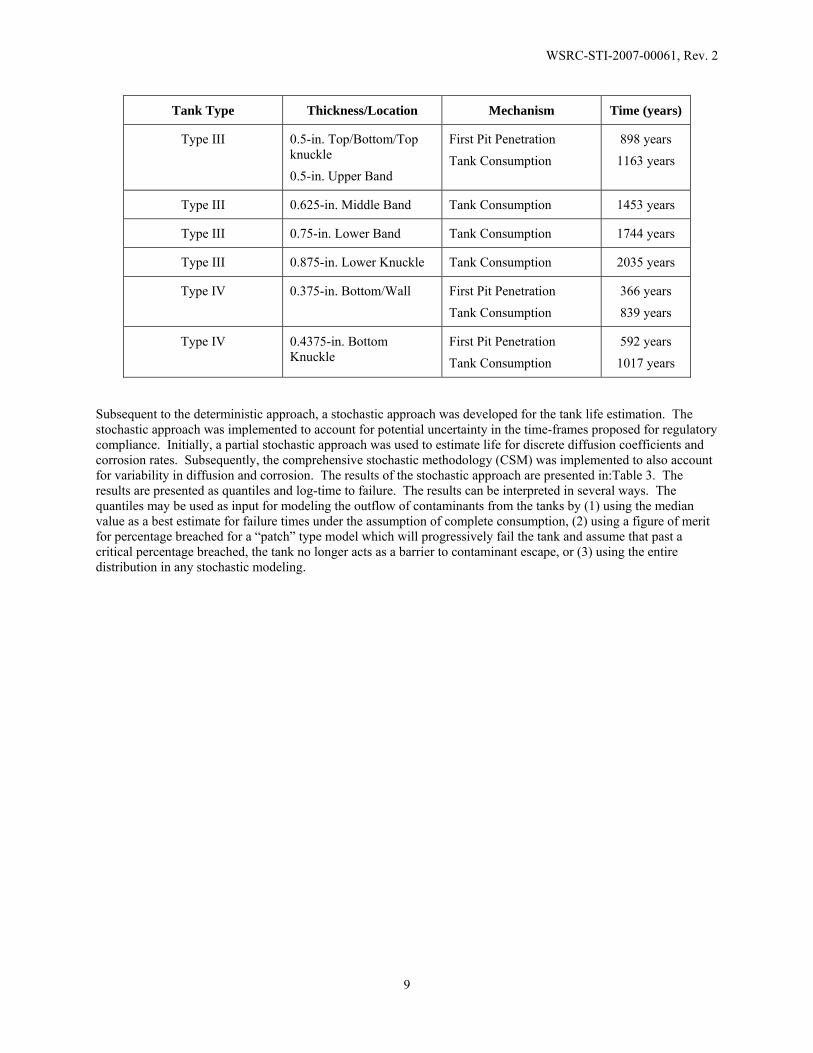
Table 2: Summary of Tank Steel Life Estimation Results in Soil Conditions


Type I 0.5-in. Bottom 0.5-in. Wall

First Pit Penetration Tank Consumption


WSRC-STI-2007-00061, Rev. 2

9


Type III 0.5-in. Top/Bottom/Top knuckle 0.5-in. Upper Band



Type III 0.625-in. Middle Band Tank Consumption 1453 years

Type III 0.75-in. Lower Band Tank Consumption 1744 years

Type III 0.875-in. Lower Knuckle Tank Consumption 2035 years

Type IV 0.375-in. Bottom/Wall First Pit Penetration Tank Consumption

366 years 839 years

Type IV 0.4375-in. Bottom Knuckle



Subsequent to the deterministic approach, a stochastic approach was developed for the tank life estimation. The stochastic approach was implemented to account for potential uncertainty in the time-frames proposed for regulatory compliance. Initially, a partial stochastic approach was used to estimate life for discrete diffusion coefficients and corrosion rates. Subsequently, the comprehensive stochastic methodology (CSM) was implemented to also account for variability in diffusion and corrosion. The results of the stochastic approach are presented in:Table 3. The results are presented as quantiles and log-time to failure. The results can be interpreted in several ways. The quantiles may be used as input for modeling the outflow of contaminants from the tanks by (1) using the median value as a best estimate for failure times under the assumption of complete consumption, (2) using a figure of merit for percentage breached for a “patch” type model which will progressively fail the tank and assume that past a critical percentage breached, the tank no longer acts as a barrier to contaminant escape, or (3) using the entire distribution in any stochastic modeling.

WSRC-STI-2007-00061, Rev. 2

10

Table 3: Life Estimation Results from Comprehensive Stochastic Approach

Type I Tanks Time to Failure Type III Tanks Time to Failure Time to IV Tanks Failure

0

10000

20000

30000

40000

50000

Log (Time to Failure)

2

3

4

Quantiles 100.0% maximum 52887 99.5% 46227 97.5% 36154 90.0% 23481 75.0% quartile 14679 50.0% median 7630 25.0% quartile 1925 10.0% 115 2.5% 55 0.5% 51 0.0% minimum 49

Moments Mean 9982.4153 Std Dev 9791.9605 Std Err Mean 8.8182837 upper 95% Mean 9999.6988 lower 95% Mean 9965.1317 N 1233023

0

10000

20000

30000

40000

50000


2

3

4

Quantiles 100.0% maximum 5293799.5% 4649497.5% 3675490.0% 2412375.0% quartile 1528950.0% median 827225.0% quartile 339710.0% 2132.5% 590.5% 530.0% minimum 49

Moments Mean 10650.171Std Dev 9763.8428Std Err Mean 8.7929618upper 95% Mean 10667.405lower 95% Mean 10632.937N 1233023

0

10000

20000

30000

40000


2

3

4



WSRC-STI-2007-00061, Rev. 2

11

2 INTRODUCTION AND BACKGROUND

High level radioactive waste (HLW) is stored in underground storage tanks at the Savannah River Site. The SRS is proceeding with closure of the 22 tanks located in F-Area. Closure consists of removing the bulk of the waste, chemical cleaning, heel removal, and filling the tank with tailored grout formulations and severing/sealing external penetrations. A performance assessment is being developed in support of closure of the F-Tank Farm. Initially, the carbon steel construction materials of the high level waste tanks will provide a barrier to the leaching of radionuclides into the soil. However, the carbon steel liners will degrade over time, most likely due to corrosion, and no longer provide a barrier. A corrosion assessment of the F-tank farm high level waste tank primary and secondary tanks will provide the necessary inputs for the radionuclide transport modeling. The corrosion assessment began with the expected initial condition of each of the tanks at closure, and considered general and pitting corrosion once grouted.

2.1 F-Tank Farm Tank Design and Construction

The F-Tank Farm consists of Type I, Type III, IIIA, and Type IV tanks. The Type I tanks are double shell tanks with partial secondary containment encased in a concrete vault. The Type III tanks are double shell tanks with full secondary containment encased in a concrete vault. The Type IV tanks are single shell tanks with steel lined concrete vaults.

2.1.1 Type I Tanks

The Type I waste tanks were made of ASTM Type A285-50T, Grade B steel, with the nominal composition shown in Table 4. The material was melted in an open-hearth furnace, semi-killed, and the hot-rolled into plate.

Table 4: ASTM Requirements for Chemical Composition for A285-50T, Grade B Firebox Quality[1]

Composition, %

C max Mn max P max S max For plates ≤ 0.75” thickness

0.2* 0.8 0.035 0.04

*C = 0.22 wt.% for plate of 0.75”< thickness ≤ 2”

Type I tanks (shown in Figure 1) have a nominal capacity of 750,000 gallons, are 75 feet in diameter, and 24.5 feet high. The primary tanks are a closed cylindrical tank with flat top and bottom constructed from 0.5-in. thick steel plate. The top and bottom are joined to the cylindrical sidewall by curved knuckle plates. The tanks are constructed with a top weld to the top of the tank, middle welds between plates, and bottom welds to the bottom of the plate. A 5-foot high steel pan provides partial secondary containment for the tanks and a concrete vault encompassing the primary tank and the steel pan provides additional containment. The Type I tanks are not stress relieved.

Figure 1: Type I Tank

WSRC-STI-2007-00061, Rev. 2

12

The primary tank rests on a three inch grout layer between the primary tank bottom and the secondary tank bottom. The secondary tank rests on the base slab.

2.1.2 Type III and Type IIIA Tanks

The most recently constructed tanks, designated Type III or IIIA, were built from hot rolled ASTM A516-Grade 70 or hot-rolled ASTM A537-Class 1 normalized steel. The normalizing heat treatment (analogous to annealing) optimizes notch toughness and hence increases resistance to brittle fracture. The nominal compositions according to ASTM Standards are shown in Table 5.

Table 5: Nominal Compositions of A516-70 and A537-Cl.1[2,3]

Steel Specification Cmax (wt%) Mnmax (wt%) Pmax (wt%) Smax (wt%)

A516 – Grade 70 t ≤ 0.5in. 0.5 < t ≤0.2 in.

0.27 0.28

0.6 – 0.9 0.6 – 1.2

0.035 0.035

0.035 0.035

A537 – Class 1 0.24 t ≤ 1.5in. 0.7 – 1.35 0.035 0.035

Each tank (as shown in Figure 2) is 85 feet in diameter and 33 feet high with a capacity of 1,300,000 gallons. Each primary vessel is made of two concentric cylinders joined to washer-shaped top and bottom plates by curved knuckle plates. The plates used to form the primary were of varying thicknesses as summarized in Table 6. The secondary vessel is 90 feet in diameter and 33 feet high (i.e., the full height of the primary tank) and is nominally 0.375-in. thick steel.

Figure 2: Type III High Level Waste Tank Schematic

The primary tank sits on a 6-in. bed of insulating grout within the secondary containment vessel. The grout bed is grooved radially so that ventilating air can flow from the inner annulus to the outer annulus. Any liquid leaking from the tank bottom or center annulus wall would move through the slots and would be detected at the outer annulus. The secondary vessel is 5 feet larger in diameter than the primary vessel, with an outer annulus 2.5-ft. wide. The secondary vessel is made of 0.375-in. steel throughout. Its sidewalls rise to the full height of the primary tank. The nested two-vessel assembly is surrounded by a cylindrical reinforced concrete enclosure with a 30-in. wall. The enclosure has a 48-in., flat, reinforced concrete roof which is supported by the concrete wall and a central column that fits within the inner cylinder of the secondary vessel.

WSRC-STI-2007-00061, Rev. 2

13

Table 6: Thickness of Plates Used in Type III Tanks

Plate Thickness (in.) Top and Bottom 0.5 Outer Cylinder Wall Upper Band Middle Band Lower Band

0.5

0.625 0.75

Inner Cylinder Wall Upper Band Lower Band

0.5

0.625 Lower Knuckle Outer Cylinder Inner Cylinder

0.875 0.625

2.1.3 Type IV Tanks

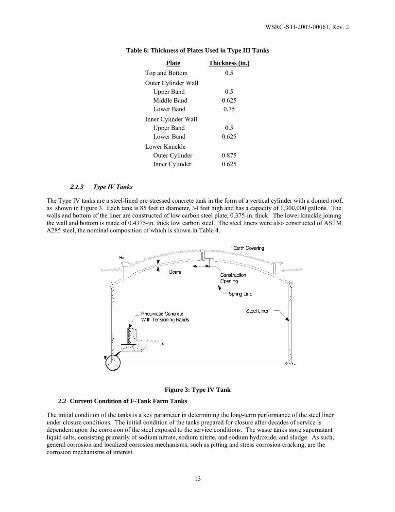
The Type IV tanks are a steel-lined pre-stressed concrete tank in the form of a vertical cylinder with a domed roof, as shown in Figure 3. Each tank is 85 feet in diameter, 34 feet high and has a capacity of 1,300,000 gallons. The walls and bottom of the liner are constructed of low carbon steel plate, 0.375-in. thick. The lower knuckle joining the wall and bottom is made of 0.4375-in. thick low carbon steel. The steel liners were also constructed of ASTM A285 steel, the nominal composition of which is shown in Table 4.

Figure 3: Type IV Tank

2.2 Current Condition of F-Tank Farm Tanks

The initial condition of the tanks is a key parameter in determining the long-term performance of the steel liner under closure conditions. The initial condition of the tanks prepared for closure after decades of service is dependent upon the corrosion of the steel exposed to the service conditions. The waste tanks store supernatant liquid salts, consisting primarily of sodium nitrate, sodium nitrite, and sodium hydroxide, and sludge. As such, general corrosion and localized corrosion mechanisms, such as pitting and stress corrosion cracking, are the corrosion mechanisms of interest.

WSRC-STI-2007-00061, Rev. 2

14

2.2.1 Service-Induced Corrosion Mechanisms

General corrosion of the waste tank steels in high pH environments that are typical of waste tanks (i.e. greater than 11) is considered insignificant.[4] This general corrosion of the waste tanks has been measured and validated through a comprehensive in-service inspection program and laboratory testing. Steel thickness measurements made using ultrasonic techniques indicated that there has been no general thinning of the waste tanks.[5] Corrosion coupons immersed in various tanks for approximately 15 years also showed little evidence of general corrosion.[6,7]

Localized corrosion in the forms of pitting and stress corrosion cracking were determined to be the two most significant and likely degradation mechanisms. Pitting is a form of extremely localized corrosion that leads to the creation of small holes in the metal, due to breakdown in passive film on metal surfaces. The morphology of pits in low carbon steel tends to be broad and shallow, with low aspect ratios. The stochastic nature of pitting typically leads to a statistical treatment of the data to determine significance.

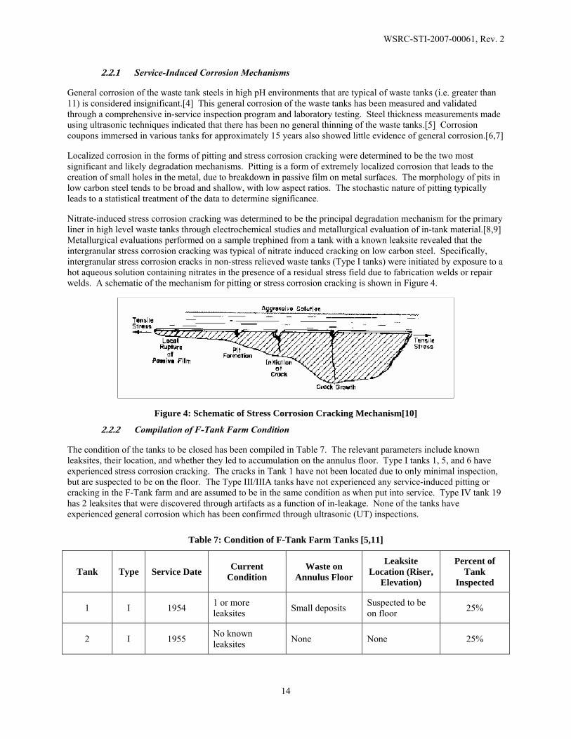
Nitrate-induced stress corrosion cracking was determined to be the principal degradation mechanism for the primary liner in high level waste tanks through electrochemical studies and metallurgical evaluation of in-tank material.[8,9] Metallurgical evaluations performed on a sample trephined from a tank with a known leaksite revealed that the intergranular stress corrosion cracking was typical of nitrate induced cracking on low carbon steel. Specifically, intergranular stress corrosion cracks in non-stress relieved waste tanks (Type I tanks) were initiated by exposure to a hot aqueous solution containing nitrates in the presence of a residual stress field due to fabrication welds or repair welds. A schematic of the mechanism for pitting or stress corrosion cracking is shown in Figure 4.

Figure 4: Schematic of Stress Corrosion Cracking Mechanism[10]

2.2.2 Compilation of F-Tank Farm Condition

The condition of the tanks to be closed has been compiled in Table 7. The relevant parameters include known leaksites, their location, and whether they led to accumulation on the annulus floor. Type I tanks 1, 5, and 6 have experienced stress corrosion cracking. The cracks in Tank 1 have not been located due to only minimal inspection, but are suspected to be on the floor. The Type III/IIIA tanks have not experienced any service-induced pitting or cracking in the F-Tank farm and are assumed to be in the same condition as when put into service. Type IV tank 19 has 2 leaksites that were discovered through artifacts as a function of in-leakage. None of the tanks have experienced general corrosion which has been confirmed through ultrasonic (UT) inspections.

Table 7: Condition of F-Tank Farm Tanks [5,11]

Tank Type Service Date Current Condition

Waste on Annulus Floor

Leaksite Location (Riser,

Elevation)

Percent of Tank

Inspected

1 I 1954 1 or more leaksites Small deposits Suspected to be

on floor 25%

2 I 1955 No known leaksites None None 25%

WSRC-STI-2007-00061, Rev. 2

15





Elevation)

Percent of Tank

Inspected



5 I 1959 18 leaksites ~ 7 gallons

NE 94-in. SSE 31-in. SSE 31-in. SSE 58-in. SSE 84-in. S 62-in. S 62-in. SW 72-in. SW 84-in. W 24-in. W 35-in. W 53-in. W 53-in. W 76-in. W 87-in. W 115-in. N 24-in. N 45-in.

75%

6 I 1964 6 leaksites ~ 92 gallons ~ 1-in. dried waste

W 129-in. WSW 145-in. NW 165-in. NW 233-in. NW 233-in. NW 233-in.

73%



17 IV 1961 Closed

18 IV 1959 No known leaksites N/A None N/A

19 IV 1961 2 leaksites N/A SW 317-in. ESE 330-in. N/A

20 IV 1960 Closed

25 IIIA 1980 No known leaksites None None 100% Visual

WSRC-STI-2007-00061, Rev. 2

16





Elevation)

Percent of Tank

Inspected




33 III 1969 No known leaksites None None 100% Visual

34 III 1972 No known leaksites None None 100% Visual





2.2.3 Stress Corrosion Crack Opening Area

A key input parameter to the performance assessment with respect to the current condition of the tanks is the calculation of the opening area of the stress corrosion cracks present in the Type I tanks. The crack opening area can be used for immediate water paths through the tank liner for water and consequent radionuclide release. However, the COA is known to be very small in comparison to the surface area of the tank.

The crack opening area (COA) is a complex function of the tank geometry, crack length, applied stress and the residual stresses. A fracture mechanics approach was taken to determine the crack opening area of each of the cracks.[12] In this case for a closed tank, it is assumed that only the residual stresses will contribute the driving force for crack opening. The grout in the closed condition of the tank is assumed not to stress the tank wall.

The stress corrosion cracking in the tanks is known to be perpendicular to the welds in the tank. The two cases studied here are for the horizontal welds and the vertical welds. Cracks emanating from the horizontal welds can be modeled as axial cracks in a cylinder, while cracks from vertical welds can be modeled as circumferential flaws in a cylinder.

Figure 5 shows the schematic for the axial flaw in a cylinder followed by a description of the COA calculation.

WSRC-STI-2007-00061, Rev. 2

17

Figure 5: Axial Flaw in a Cylinder

The crack opening area, ‘A’, for this geometry is calculated through the following approach[12]:

( ) ( )λπσ GRtE

A ⋅= 2

Where: A = Crack Opening Area (in.2) E = Young’s Modulus (psi) σ = Maximum Hoop Stress (psi) G(λ) = Function of the shell parameter ‘λ’

And:

tRP=σ

Rta

=λ

( ) 42 625.0 λλλ +=G

The hoop stress due to residual stress can be indirectly calculated by equating the stress intensity caused by residual stresses to an equivalent hoop stress as follows[13]:

tK y ⋅= πσ38.0

where: K = Stress Intensity (psi-in1/2) σy = Yield Stress (psi) t = thickness (in.)

R = Radius to Inner Surface (in.)

a = crack length (in.)

t = thickness (in.)

P = loading (psi)

WSRC-STI-2007-00061, Rev. 2

18

225.11 λπσ

+⋅⋅=

aK

eq

where: σeq = Equivalent hoop stress (psi)

It is conservatively assumed that the residual stresses in the tank are equivalent to the yield stress, the theoretical limit. Through substitution, the COA can be calculated by:

( )42 625.02 λλπσ

+= RtE

A eq

The crack was also modeled as a circumferential flaw emanating from a vertical weld, as shown in Figure 6.

Figure 6: Circumferential Flaw in a Cylinder [12]

The crack opening area can be directly calculated by[12]:

( )⎟⎠⎞

⎜⎝⎛ −+−= 2

42

1124

ααπσE

tA y where:

ta2

=α

Where: A = Crack Opening Area (in.2) E = Young’s Modulus (psi) σy = Yield Stress (psi) t = thickness (in.) α = dimensionless crack size a = crack length (in.)

The two geometry parameters for input into the calculations are the length of a crack, and the tank wall thickness. As such, the crack opening area was calculated for the various thicknesses of tank walls and the maximum reference crack size known for the F-Area tanks. The calculations were made only for Type I and Type IV tanks. Laboratory and inspection observations show that cracks grow perpendicular to the weld and are contained with the residual stress fields of the weld areas in the F-Area tanks. As such, a maximum length of 6-in. is used as the reference flaw size and is considered to be the conservative assumption.[14] (NOTE: There are several anomalous crack lengths within the Type II tanks, but are not considered relevant for the Type I tanks) A summary of the inputs and materials properties used for the calculations are as follows:

a = crack length (in.)

WSRC-STI-2007-00061, Rev. 2

19

Crack length, ‘a’, = 6-in. Young’s Modulus, ‘E’ = 30000000 psi Yield stress, ‘σy’ (ASTM A285) = 27000 psi Thickness, ‘t’ = 0.375-in. (Type IV tanks) = 0.4375-in. (Type IV tanks) = 0.5-in. (Type I tanks) Radius, ‘r’ = 900-in. (Type I tanks) = 1020-in. (Type IV tanks)

The results of the calculation are shown in Table 8.

Table 8: Crack Opening Area for Stress Corrosion Cracks

Tank Type Wall Thickness (in.) Axial COA (in.2) Circumferential COA (in.2) Type I 0.5 0.007 0.006

Type IV 0.375 0.007 0.008 Type IV 0.4375 0.008 0.01

The crack opening areas for each of the stress corrosion cracks is minimal, and consequently will have minimal impact in the possibility of flow when compared to the total surface area of the tank.

3 TANK STEEL LIFE ESTIMATION TECHNICAL APPROACH

The life of the primary and secondary tank steels and performance as a barrier to radionuclide escape is dependent upon the active corrosion mechanisms on the steel under closure conditions. General corrosion, pitting, and stress corrosion cracking were the primary corrosion mechanisms considered in the tank steel life estimation. These corrosion mechanisms were considered as a function of the specific environment that each surface of the tank will be exposed to. General corrosion and pitting were considered with exposures to the grouted conditions and soils when the grout is not present. These data can then be used as input into the modeling effort.

3.1 Tank Exposures

An accurate representation of the exposure conditions of the tanks is critical to the life estimation of the tank steel. Each of the sections of the tank will be exposed to different chemical environments under closure conditions. A summary of the exposure for each of the Type I, III, and Type IV tank sections are shown in Table 9 - 11 respectively. The exposures of the tank steel can be the initial concrete/grout during construction, the closure grout or the contamination zone, i.e. undissolved solids in the bottom of the tank. The closure condition does not credit the complete encapsulation of this residual by the grout, therefore, the bottom of the tank will be permanently exposed to the contamination zone.

Table 9: Type I Tank Steel Exposure in Closure Configuration

Tank Wall Location Exposure Primary Bottom – Internal Contamination Zone Primary Bottom – External Initial Grout Pad

Primary Wall – Internal Closure Grout Primary Wall – External Closure Grout

Secondary Bottom – Internal Grout Pad Secondary Bottom – External Concrete Vault (Base Slab)

Secondary Wall – Internal Closure Grout Secondary Wall – External Concrete Vault

WSRC-STI-2007-00061, Rev. 2

20

Tank Wall Location Exposure Top – Internal Closure Grout Top - External Concrete Vault

Table 10: Type III/IIIA Tank Steel Exposure in Closure Configuration

Tank Wall Location Exposure Primary Bottom – Internal Contamination Zone Primary Bottom – External Initial Insulating Grout

Primary Inner Cylinder Wall – Internal Closure Grout Primary Inner Cylinder Wall – External Closure Grout

Secondary Bottom – Internal Initial Grout Pad Secondary Bottom – External Concrete Vault (Base Slab)

Secondary Wall – Internal Closure Grout Secondary Wall – External Concrete Vault

Top – Internal Closure Grout Top - External Concrete Vault

Table 11: Type IV Tank Steel Exposure in Closure Condition

Tank Wall Location Exposure Primary Bottom – Internal Contamination Zone Primary Bottom – External Initial Grout

Tank Wall – Internal Closure Grout Tank Wall –External Concrete Vault

The exposure of the tank surfaces is variable for the tank walls and bottom, and from the outside of the tank and within the inside. The exposure of the tank for purposes of this life estimation was simplified to a concrete liner in a concrete vault grouted on the interior. The primary corrosion mechanisms considered were due to (1) exposure of the interior of the tank bottom to the contamination zone, and (2) exposure of the exterior of the walls, and the interior to corrosion mechanisms typical within concrete, i.e. chloride attack and carbonation. The mechanisms of corrosion of steel within a concrete matrix are a function of the diffusion coefficients of chloride, oxygen, and carbon dioxide. As such, it was conservatively assumed that diffusion of these species through the minimum concrete vault dimension subjected the entire interior and exterior surface of the tank walls and bottom to the degraded state. In addition, credit was taken only for the primary wall liner, and not for the secondary tank. A summary of the modeled state is shown in Figure 7.

WSRC-STI-2007-00061, Rev. 2

21

Figure 7: Model of Tank in Closed Condition for Lifetime Assessment.

3.2 Corrosion Mechanism in Contamination Zone

Corrosion of the steel exposed to the contamination zone is a function of the chemistry of the undissolved solids in the residual on the tank bottom. Corrosion of the steel exposed to the contamination zone is most susceptible to nitrate induced corrosion. During corrosion in nitrate solutions, carbon steel reacts anodically by :

3Fe + 4H2O → Fe3O4 +8H+ + 8e-

and the cathodic reactions sum to:

NO3- + H2O + 2e- → NO2

- + 2OH-

As such the nitrate induced corrosion can be inhibited by inhibiting the cathodic reaction through nitrite or hydroxide, the approach used for the chemistry control program during service of the tanks.[10] The addition of hydroxide also maintains the high pH associated with passivity and low corrosion rates.

The ratio of the concentration of inhibitor species (nitrite and hydroxide) to aggressive species (nitrate + chloride), referred to as the R-value, was utilized to assess the potential for corrosion by exposure to the contamination zone.[15] High R-values indicate that the potential for corrosion is minimal, while low R-values indicate a high potential for corrosion due to insufficient inhibitor concentrations. The expected residual material inventory was used to calculate R-values for the chemistry in the contamination zone, under the conservative assumption that the dried solids were in solution.[16] The molarity of the sodium nitrate and sodium hydroxide (assuming 1kg of sludge) were calculated using:

[ ]SoluteMWSludgeL

SludgegalSludgegalSludgeg

gSludgeAmountgSoluteAmountMionConcentrat 1

785.31

1885

][][

×××=

where: Density of Residuals = 885g/1 gal sludge (based on Reference 16) Solute = NaNO3 + NaCl or NaOH MW = Molecular Weight (NO3

- = 62g/mol, Cl- = 35 g/mol, OH- = 17g/mol)

The results of the calculations, shown in Table 12, show that the tank bottom will undergo minimal corrosion under these highly alkaline conditions, and the conservative assumption that the residuals are in solution. The general corrosion rate in these conditions is estimated at 0.04 mil/yr (1µm/year).[17]

Closure Grout

Contamination Zone

Concrete Vault

WSRC-STI-2007-00061, Rev. 2

22

Table 12: R-Value of Contamination Zone Exposure

Tank R-Value

1 5.47

2 4.36

3 3.94

4 9.67

5 5.31

6 12.39

7 3.44

8 3.87

17 3.18

18 4.51

19 0.24

20 3.18

25 3.19

26 3.19

27 3.19

28 3.19

33 4.53

34 12.40

44 4.45

45 3.19

46 3.19

47 3.19

3.3 Corrosion Mechanisms in Concrete/Grout

Corrosion of steel exposed to concrete/grout occurs by a complex mechanism through metal dissolution at the concrete/metal interface. This interfacial chemistry is controlled by the initial construction characteristics and the grout formulations. In general, high quality concrete prevents corrosion of the steel by: (1) forming a passive oxide on the steel surface, (2) maintaining a high pH environment, and (3) providing a matrix resistant to diffusion of aggressive species. The passivity of the steel at the interface can be controlled by the dynamic characteristics of the “pore water” (interstitial solution ) within the concrete.[18] The passivity is maintained at the high pH environments in the region of water stability. However, as pore water characteristics change with the introduction of chlorides or

WSRC-STI-2007-00061, Rev. 2

23

carbon dioxide, the passive film on the steel may break down. The two major causes of corrosion of steel exposed to concrete are carbonation and chloride induced breakdown of the passive film. The passivity of the steel is lost when the pH is lowered below 9 (by carbonation) or a critical chloride concentration is reached at the concrete metal interface.[19]

The initial concrete material quality is potentially the most significant factor in the prevention of corrosion of the steel in contact with as-constructed vault. A review based upon several site specifications which relate concrete materials to construction requirements is presented here.[20] The Type I and Type III tanks have a grout layer between the primary and secondary containment, and the base slab upon which the secondary tank rests. The Type IV tanks have a concrete vault that was formed by the “shotcrete” technique.

The cement density, water-to-cement (WCR) ratio, and content are key parameters for cement content and type. The cement density of the mixture has been calculated to be 590 lbs/yd3, consistently above the minimum 490 lbs/yd3.[21] The water to cement ratio was calculated to be 0.6, which is relatively high. However, water proofing membranes were used in the HLW tanks to prevent chloride intrusion from external sources. The concrete may have been constructed with either Portland cement, 75% Portland cement with 25% slag cement, or 85% Portland cement and 15% fly ash. The use of blended cements may affect the corrosion rate due to reduced alkalinity. However, these cements also decrease the permeability to anions that potentially cause pitting in the steel, i.e. chloride by reducing the water to cement ratio.[22]

It is assumed in this case that a passive layer forms on the steel surface spontaneously when in contact with the alkaline cement. This corrosion rate in this inactive state is estimated to be 0.04 mils/year (1µm/year). [23] This corrosion rate corresponds to a passive current density (Icorr) of 0.09 µΑ/cm2, which is just below the typical threshold used for the passive state, i.e. Icorr < 0.1 µA/cm2.[24] Although there is a broad variety of literature values for rebar steel, the passive current densities for the buried steel/concrete structures are reported to be < 0.01 µA/cm2.

3.3.1 Carbonation

Carbonation is the process through which pore water pH reduces dramatically due to the conversion of the calcium hydroxide to calcium carbonate through reaction with carbon dioxide, as shown in the following reaction:[25]

( ) OHCaCOCOOHOHCa 23222 2+⇒++

The active corrosion of the steel exposed to the low pH solution at the carbonation front will then proceed due to the formation of non-protective oxides.

The carbonation of concrete is a complex function of the permeability of the concrete, relative humidity, and the carbon dioxide availability. A rigorous mechanistic model for the carbonation of concrete considering mass transport, chemical reaction, and reaction kinetics has been developed.[26] The model can be simplified to the following approximation for estimation of carbonation of the tank concrete vault under the listed appropriate assumptions:[27]

21

2 ⎟⎟⎠

⎞⎜⎜⎝

⎛=

g

gwi CC

DX

where: X = carbonation depth (cm) Di = intrinsic diffusion coefficient of CO2 in concrete (cm2/s) Cgw = total inorganic carbon in ground water or soil moisture (mole/cm3)

Cg = Ca(OH)2 bulk concentration in concrete solid (mole/cm3) t = time (s)

This approach is appropriate for this case since subsurface concrete vaults are typically water saturated, and thus the CO2 transport is in the aqueous phase.

WSRC-STI-2007-00061, Rev. 2

24

The carbonation calculations were made with the following inputs:

Parameter Value Type I Tank Minimum Concrete Vault Dimension 22-in.

Type III Tank Minimum Concrete Vault Dimension 30-in. Type IV Tank Minimum Concrete Vault Dimension 4-in.

Di (CO2) 1E-8 cm2/sec ≤ Di ≤ 1E-3 cm2/sec

Cgw (as soil moisture content) 1.93E-7 mol/cm3 [28] Cg 0.02 mol/cm3 [29]

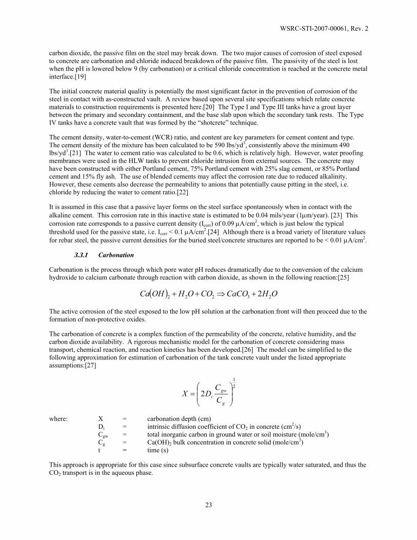
The results of the carbonation calculations are shown in Figure 8. Assuming that the diffusion coefficient remains constant, carbonation is not expected to be an issue in the Type I and III/IIIA tanks within 10,000 years if the diffusion coefficient remains below 1E-3 cm2/sec. However, for a diffusion coefficient of 1E-4 cm2/sec, the carbonation front can reach the tank/steel interface at 1700 years for the Type IV tanks.

Time to Carbonation of Concrete/Tank Steel Interface

1.E+02

1.E+03

1.E+04

1.E+05

1.E+06

1.E+07

1.E+08

1.E+09

1.E+10

1.E-08 1.E-07 1.E-06 1.E-05 1.E-04 1.E-03

Diffusion Coefficient (cm2/sec)

Tim

e (y

ears

)

Type I TanksType III/IIIA TanksType IV Tanks

Figure 8: Time to Carbonation Front to Reach Concrete/Tank Steel Interface as a Function of Diffusion Coefficient.

The effect of the carbonation front is essentially the reduction of the pH into a regime where the steel is susceptible to corrosion. The corrosion rate of steel exposed to aerated solutions between pH 4 and 10 is relatively independent of the pH of the environment, as shown in Figure 9. In this pH range, the corrosion rate is governed largely by the rate at which oxygen reacts with absorbed atomic hydrogen, thereby depolarizing the surface and allowing the reduction reaction to continue. The corrosion rate within this pH range can be estimated at 10 mils/year.

WSRC-STI-2007-00061, Rev. 2

25

Figure 9: Effect of pH on the Corrosion of Iron Exposed to Aerated Water at Room Temperature [30]

3.3.2 Chloride Induced Corrosion

Chloride induced corrosion is due to the breakdown of the passive film, thereby indicating that chloride diffusion is the rate controlling step for corrosion initiation. Once initiation has occurred, the oxygen diffusion to the steel surface will control the corrosion propagation. As such, the chloride induced corrosion of the tank steel will be determined by first calculating the time to initiation, then calculating the corrosion rate.

Two methodologies are available to estimate the chloride induced initiation of corrosion of steel structures encased in concrete:

• An empirical model to determine the corrosion initiation time[31]:

[ ] 42.0

22.1129−⋅

⋅=

ClWCRtt c

initiation

where: tinitiation = time required for initiation (years) tc = thickness of the concrete cover (in.) WCR = water-to-cement ratio [Cl-] = chloride concentration in the groundwater (ppm)

• Modeling the critical [Cl-]/[OH-] ratio for corrosion initiation, where a critical chloride to hydroxide ratio is necessary to initiate pitting.[32] This critical ratio has been proposed to be 0.6, but is known to decrease with decreasing pH. In this methodology, the chloride diffusivity would be calculated per Fick’s law, similar to carbonation.

The chloride threshold value is controversial, since it is influenced by various factors, such as cement type, mixture proportions of concrete, relative humidity, temperature, pH value of pore solution, sulfate content. As such, the degradation due to chloride will be estimated with the first empirical option, a broadly accepted methodology.

The corrosion rate of propagation can be calculated by relating oxygen diffusion through the concrete to the corrosion reaction. The general corrosion reaction is:

( )322 43

23 OHFeOOHFe ⇒++

WSRC-STI-2007-00061, Rev. 2

26

The oxygen diffusion through the concrete is represented by:

XC

DN gwiO ∆

=2

where: NO2 = flux of oxygen through concrete (mol/s/cm2) Di = oxygen diffusion coefficient in concrete (cm2/sec)

Cgw = concentration of oxygen in groundwater (mol/cm3) ∆X = Depth of concrete (cm)

The corrosion rate can then be calculated by:

Fe

FeOcorrosion

MNRρ23

4=

where: MFe = molecular weight of iron (56 g/mol) ρFe = density of iron (7.86 g/cm3)

The inputs used for calculating the chloride induced attacks are as follows:

Parameter Value Type I Tank Minimum Concrete Vault Dimension 22-in.

Type III Tank Minimum Concrete Vault Dimension 30-in. Type IV Tank Minimum Concrete Vault Dimension 4-in.

WCR 0.6 [Cl-] 2-100 ppm

Di (Oxygen) 1E-8 cm2/sec ≤ Di ≤ 1E-3 cm2/sec [33] Cgw (Oxygen) 7.25 mg/L [34]

The time to initiation of chloride induced attack as a function of the groundwater [Cl-] concentration is shown in Table 13 and Figure 10. The typical chloride concentration is 2-3 ppm.[35]

WSRC-STI-2007-00061, Rev. 2

27

Table 13: Initiation Time for Chloride Induced Corrosion

[Cl-] ppm tinitiation (yrs) Type I 2 6978

5 4749 10 3550 50 1806 100 1350

Type III 2 10188 5 6934 10 5182 50 2636 100 1970

Type IV 2 872 5 593 10 444 50 226 100 169

Chloride Induced Corrosion Initiation Time

0

2000

4000

6000

8000

10000

12000

0 20 40 60 80 100 120

[Cl-] ppm

tiniti

atio

n (ye

ars)

Type I

Type III

Type IV

Figure 10: Initiation Time for Chloride Induced Attack as a Function of Chloride Concentration in Groundwater.

WSRC-STI-2007-00061, Rev. 2

28

It is conservatively assumed that once chloride reaches the tank-steel interface through the minimum thickness of the vault, the entire surface of the tank is subject to the higher corrosion rate from the interior and exterior.

The calculated corrosion rate as a function of oxygen diffusivity is shown in Figure 11. For purposes of corrosion rate calculations, the critical oxygen diffusivity at which the corrosion rate will be greater than 0.04 mils/year corrosion rate is as follows:

• Type I Tank: 8.29x10-5 cm2/sec

• Type III Tank: 1x10-4 cm2/sec

• Type IV Tank: 1.51x10-5 cm2/sec

The corrosion rate can be conservatively assumed to be 0.04 mils/year (typical of steel in contact with concrete) when the diffusion values are lower than the critical values. However, when the diffusion rate is greater, the corrosion rate must be calculated as shown in Figure 11.

Corrosion Rate As a Function of Oxygen Diffusivity

1.E-06

1.E-05

1.E-04

1.E-03

1.E-02

1.E-01

1.E+00

1.E+01

1.E-08 1.E-07 1.E-06 1.E-05 1.E-04 1.E-03

Oxygen Diffusivity (cm2/sec)

Cor

rosi

on ra

te (m

ils/y

ear)

Type I TanksType III TanksType IV Tanks

Figure 11: Corrosion Rate as a Function of Oxygen Diffusivity Once Chloride Induced Corrosion is Initiated.

It is assumed that the entire tank interior and exterior is subject to the accelerated corrosion rate when chloride induced corrosion in initiated.

3.3.3 Microcell/Macrocell Corrosion

Microcell/Macrocell corrosion, or “galvanic corrosion”, were also considered in the life estimation scheme. Microcell corrosion occurs when different parts of the same metal embedded in concrete corrode at varying rates, i.e. the cathodic and anodic half-cell reactions occur at different parts of the same metal. Macrocell corrosion occurs where metal embedded in a concrete can corrode preferentially due to contact with either another metal or a

WSRC-STI-2007-00061, Rev. 2

29

different environment.[36] Galvanic corrosion mechanisms are typical of concrete that has been patch repaired. The patch repairs may lead to conditions where variances in the initial concrete vs. the patch concrete, or variations in the initial steel vs. the repair steel may lead to conditions promoting galvanic corrosion.[37] These galvanic corrosion mechanisms were determined not to be active in the closed conditions of the tank as there will be no repair patches to the concrete or the rebar.

3.3.4 Microbially Induced Corrosion

Microbially induced corrosion (MIC) is the corrosion of steel due to microorganic films/deposits or the chemicals formed from the metabolic products of the microorganisms. The corrosion of the exposed metal can be accelerated by: (1) consuming oxygen and consequently creating oxygen concentration cells; (2) producing acids and reducing pH; (3) consuming hydrogen and thereby depolarizing cathodic areas, (4) producing elemental sulfur and hydrogen sulfide, (5) adsorbing and concentrating chloride ions, or (6) removing dissolved iron, thereby stimulating further iron dissolution. MIC is typically associated with stagnant water conditions ideal for the growth of such mechanisms. The potential for MIC in the closed tank configuration was determined to be linked to the alkalinity of the surrounding concrete. The high alkalinity of the surrounding concrete is considered to prevent the formation of microorganisms that may lead to corrosion.[38,39] However, as the carbonation mechanism proceeds through the concrete, MIC may become active. As such, modeling of the carbonation mechanism and the consequent corrosion rate due to reduced pH was determined to account for the potential for MIC.

3.4 Corrosion of Tank Steel Exposed to Soil

The corrosion of tank steel exposed to soil was also estimated under the most conservative scenario in which the concrete vault has completely degraded. Corrosion in soil is a complex function of the soil characteristics including resistivity, aeration, drainage, availability of moisture, and pH. The mechanism for soil corrosion is differential aeration which leads to anode formation at areas of low oxygen and water permeability, while the cathode forms at areas of high permeability. Soil can lead to localized corrosion or general corrosion, which are both considered in this analysis. The analysis has been reproduced from reference 40 and extended to the Type I/III tanks. [40]

3.4.1 General Corrosion

An understanding of the soil characteristics is key in determining the corrosion response of the tank steel in soil. The database of metallic corrosion compiled by the National Bureau of Standards was used to determine the general corrosion rate to be used for the calculation.[41] A survey of the data revealed that soil conditions at the Atlanta test site, shown in Table 14, are comparable and yet conservative with respect to resistivity and pH in comparison to SRS soils.

Table 14: Soil Conditions Used for Analysis

The weight-loss and maximum penetration data presented in Reference 41 for open-hearth steel plate was used to calculate the corrosion rate and maximum penetration rate, i.e. localized corrosion rate. The results are shown in Table 15.

Location Atlanta, GA Type of Soil Cecil clay loam Resistivity of Soil 17,790 ohm-cm pH of Soil 4.8 Mean Temperature 61.2°F Annual Precipitation 48.3 – in. Moisture Equivalent 33.7%

WSRC-STI-2007-00061, Rev. 2

30

Table 15: Weight Loss of Carbon Steel in Cecil Clay Loam Soil

Years Weight Loss (kg/m2) Corrosion Rate (µm/yr) Max Penetration (µm/yr)

2 0.54 (1.8 oz/ft2) 34.78 (1.37mpy) 508 (20mpy)

5.5 0.96(3.2 oz/ft2) 22.48 (0.89mpy) 351(13.82mpy)

7.6 1.18(3.9 oz/ft2) 19.83 (0.78mpy) 191 (7.5mpy)

9.5 1.02(3.4 oz/ft2) 13.83 (0.54mpy) 193 (7.58mpy)

14.3 1.21(4 oz/ft2) 10.81 (0.43mpy) 139 (5.45mpy)

The general corrosion rate and the maximum penetration are shown in Figure 12 as a function of time. The data shows that the corrosion rate decreases with time typically in a power-law relationship.

Corrosion Rate vs. Time

0.00

0.20

0.40

0.60

0.80

1.00

1.20

1.40

1.60

0 5 10 15 20

Years

Cor

rosi

on R

ate

(mpy

)

0.00

5.00

10.00

15.00

20.00

25.00

Max

imum

Pen

etra

tion

Rat

e (m

py)

General CorrosionRate

MaximumPenetration Rate

Figure 12: Corrosion Rate and Maximum Penetration Rate as a Function of Time.

The general corrosion rate of 0.4 mils/year can be used as a conservative estimate for corrosion of the tank steel exposed to the soil.

3.4.2 Pitting Corrosion

The pitting model assumes formation of a hemispherical pit and estimates the area breached based upon the maximum pit depth, the corrosion allowance, and the number of penetrating pits per container:

( )22 dhNA pb −= π

where: Ab = Area breached (m2) Np = penetrating pits per container (pits/m3) – assumed to be 5000 per m2[42] h = maximum pit depth (m) d = corrosion allowance

The maximum pit depth can be estimated by:

WSRC-STI-2007-00061, Rev. 2

31

an Akth ⎟

⎠⎞

⎜⎝⎛=

372

where: k = empirical pitting parameter (m/yrn) t = corrosion time (yr) n = empirical pitting exponent A = representative surface area (cm2) a = experimentally derived empirical coefficient

Regression analysis of pitting data yielded values of 34.49 and 0.3205 respectively for ‘k’ and ‘n’.[43] Literature values report a mean of 0.15 for exponent ‘a’.[44] Using these values, the final form of the equation is:

3205.056.56)( tmilsh =

where: h = pit depth (mils) t = corrosion time (year)

This final form will be used for tank steel life estimation.

4 TANK STEEL LIFE ESTIMATION RESULTS

The life of the tank steel was estimated for exposures to grouted conditions and also exposures to soils. The life of the tank steel was also estimated for a third condition in which a pipe of humid air may form between the grout/vault and the tank steel.

4.1 Grouted Conditions

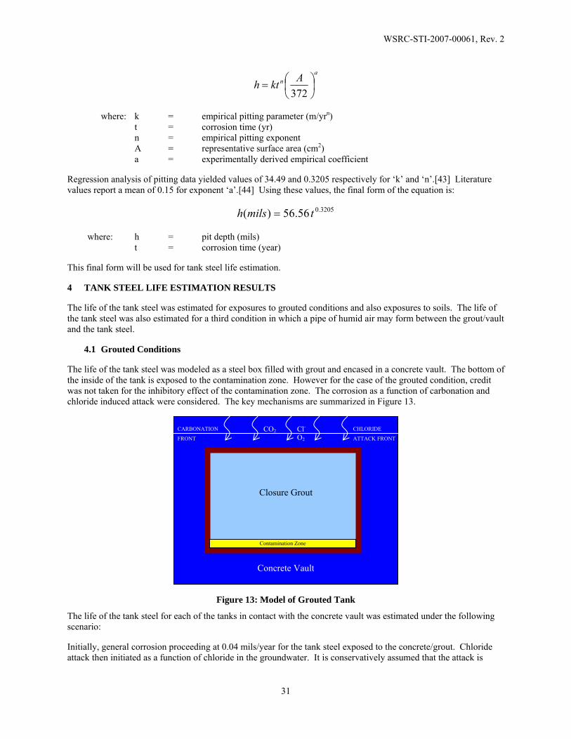
The life of the tank steel was modeled as a steel box filled with grout and encased in a concrete vault. The bottom of the inside of the tank is exposed to the contamination zone. However for the case of the grouted condition, credit was not taken for the inhibitory effect of the contamination zone. The corrosion as a function of carbonation and chloride induced attack were considered. The key mechanisms are summarized in Figure 13.

Figure 13: Model of Grouted Tank

The life of the tank steel for each of the tanks in contact with the concrete vault was estimated under the following scenario:

Initially, general corrosion proceeding at 0.04 mils/year for the tank steel exposed to the concrete/grout. Chloride attack then initiated as a function of chloride in the groundwater. It is conservatively assumed that the attack is

Closure Grout

Contamination Zone

Concrete Vault

CO2 Cl-

O2

CARBONATION

FRONT

CHLORIDE

ATTACK FRONT

WSRC-STI-2007-00061, Rev. 2

32

initiated on the both internal and external surfaces of the tank once chloride has penetrated through the thinnest section of concrete. The chloride concentration is conservatively assumed to be 10 ppm. The corrosion will then proceed at the calculated rate as a function of oxygen diffusivity as outlined in Section 3.3.2. The oxygen diffusivity is conservatively assumed to be 1x10-4 cm2/sec. The calculation conservatively assumes that oxygen is available over the entire surface once the oxygen penetrates the thinnest section of concrete, corresponding to the following corrosion rates:

• Type I Tanks - 0.0478 mils/year

• Type III Tanks - 0.04 mils/year

• Type IV Tanks - 0.26 mils/year

The corrosion rate will proceed in this scenario until the entire tank wall is converted at a critical theoretical time. The hydraulic conductivity can be assumed to be zero, until the tank wall is completely corroded.

4.1.1 Estimation of Type I Tank Steel Life Exposed to Grouted Conditions

The Type I tanks are built of 0.5-in steel for the walls as well as the tank bottom and top. It is assumed that the tank steel will corrode at an equivalent rate for every surface of the tank wall from the interior and exterior. The penetration depth due to corrosion is shown in Figure 14. The chloride penetration time is 3550 years, beyond which the corrosion rate increases from 0.04 mils/year to 0.0478 mils/year. The 0.5-in thick steel of the tank top, tank walls, and tank bottom are estimated to be consumed in 5809 years.

Corrosion of Type I Tank Exposed to Grouted Conditions

Chloride Attack Initiated at 3550

years

Penetration at 5809 years

0

0.1

0.2

0.3

0.4

0.5

0.6

0 1000 2000 3000 4000 5000 6000 7000

Time (years)

Dep

th o

f Cor

rosi

on P

enet

ratio

n (in

.)

Corrosion Rate = 0.04 mils/year


Figure 14: Type I Tank Penetration Calculation

4.1.2 Estimation of Type III Tank Steel Life Exposed to Grouted Conditions

The Type III tanks are built of 0.5-in steel for tank bottom and top. The tank wall increases in thickness from the top knuckle at 0.5-in.– 0.625-0.75-0.875-in. for the lower knuckle. It is assumed that the tank steel will corrode at an equivalent rate for every surface of the tank wall. The penetration depth due to corrosion is shown in Figure 15.

WSRC-STI-2007-00061, Rev. 2

33

The chloride penetration time is 5182 years, however, the corrosion rate is maintained at 0.04 mils/year since the corrosion rate as calculated by oxygen diffusivity is lower than this assumed minimum corrosion rate. The 0.5-in thick steel of the tank top, top knuckle, and tank bottom will be completely penetrated after 6250 years, and will increase to 10,937 years for the lower knuckle which is 0.875-in. thick. The middle plates which are 0.625-in. and 0.75-in. thick will be penetrated in 7812 and 9375 years respectively.

Corrosion of Type III Tank Exposed to Grouted Conditions

10938 years0.875-in.

9375 years0.75-in.

7813 years0.625-in.

6250 years0.5-in.

0

0.1

0.2

0.3

0.4

0.5

0.6

0.7

0.8

0.9

1

0 2000 4000 6000 8000 10000 12000

Time (years)

Dep

th o

f Cor

rosi

on P

enet

ratio

n (in

.)

Corrosion LinePenetration Time

Figure 15: Type III Tank Penetration Calculation

4.1.3 Estimation of Type IV Tank Steel Life Exposed to Grouted Conditions

The Type IV tanks are built of 0.375-in steel for the walls and bottom, with the lower knuckle constructed of 0.4375-in. It is assumed that the tank steel will corrode at an equivalent rate for every surface of the tank wall. The penetration depth due to corrosion is shown in Figure 14. The chloride penetration time is 444 years, beyond which the corrosion rate increases from 0.04 mils/year to 0.26 mils/year. The 0.375-in walls will be penetrated after 1096 years and the lower knuckle will be penetrated after 1217 years.

WSRC-STI-2007-00061, Rev. 2

34

Corrosion of Type IV Tank Exposed to Grouted Conditions

Chloride attack initiated at 444

years

1217 years, 0.4375-in.

1096 years, 0.375-in.

0

0.1

0.2

0.3

0.4

0.5

0.6

0.7

0.8

0.9

0 500 1000 1500 2000 2500

Time (years)

Dept

h of

Cor

rosi

on P

enet

ratio

n (in

.)

Corrosion Line

Penetration Time



Figure 16: Type IV Tank Penetration Calculation

4.2 Soil Conditions

The tank steel life estimation was calculated for soil exposure conditions as the conservative case-study if the concrete vault fails.

4.2.1 Estimation of Type I Tank Steel Life Exposed to Soil

The Type I tanks are built of 0.5-in steel for the walls as well as the tank bottom and top. The corrosion of the Type I tanks when exposed to soil is shown in Figure 17. The maximum pit depth and depth of general corrosion are shown as a function of time. It is estimated the first pit penetrates thru-wall at 898 years, while the general corrosion is estimated to consume the tank steel at 1163 years.

WSRC-STI-2007-00061, Rev. 2

35

Corrosion of Type I Tank Exposed to Soil

1163 Years

898 Years

0

0.1

0.2

0.3

0.4

0.5

0.6

0 200 400 600 800 1000 1200 1400

Time (years)

Dep

th o

f Cor

rosi

on P

enet

ratio

n (in

.)

General Corrosion

Pitting

Figure 17: Corrosion of Type I Tank Exposed to Soil

The percentage of the tank steel breached due to pitting was also calculated, and is shown in Figure 18. It is estimated that the tank steel wall will be consumed in 1509 years due to pitting, which is much longer than the conservative estimation used for the general corrosion calculations. Therefore, it is conservatively estimated that the general corrosion will consume the tank steel in 1163 years if exposed to soil.

Percentage Breached of Type I Tanks Exposed to Soil Due to Pitting

1509 Years

0

20

40

60

80

100

120

0 500 1000 1500 2000

Years

% B

reac

hed

Figure 18: Percentage of Type I Tank Wall Breached Due to Pitting as a Function of time.

WSRC-STI-2007-00061, Rev. 2

36

4.2.2 Estimation of Type III Tank Steel Life Exposed to Soil

The Type III tanks are built of 0.5-in steel for tank bottom and top. The tank wall increases in thickness from the top knuckle at 0.5-in.– 0.625-0.75-0.875-in. for the lower knuckle. The corrosion of the Type III tanks when exposed to soil is shown in Figure 19. The maximum pit depth and depth of general corrosion are shown as a function of time. It is estimated the first pit penetrates thru-wall at 898 years for the 0.5-in. portions of the tank, while the general corrosion is estimated to consume the 0.5-in. thick tank steel at 1163 years. The tank steel that is 0.625-in, 0.75-in, and 0.875-in. will be consumed in 1453, 1744, and 2035 years respectively. The conservatively assumed general corrosion rates are faster than those for the maximum pitting depth for longer time frames.

Corrosion of Type III Tank Exposed to Soil

2035 Years, 0.875-in.

1744Years, 0.75-in.

1453 Years, 0.625-in.

1163 Years, 0.5-in.

898 Years

0

0.1

0.2

0.3

0.4

0.5

0.6

0.7

0.8

0.9

1

0 500 1000 1500 2000 2500

Time (years)

Dep

th o

f Cor

rosi

on P

enet

ratio

n (in

.)

General Corrosion

Pitting

Figure 19: Corrosion of Type III Tank Exposed to Soil

The percentage of the tank steel breached due to pitting was also calculated, and is shown in Figure 20. It is estimated that the tank steel wall will be consumed in 1509 years due to pitting, which is much longer than the conservative estimation used for the general corrosion calculations. Therefore, it is conservatively estimated that the general corrosion will consume the 0.5-in. tank steel in 1163 years if exposed to soil.

WSRC-STI-2007-00061, Rev. 2

37

Percentage Breached of Type III Tanks Exposed to Soil Due to Pitting

1509 years

0

20

40

60

80

100

120

0 200 400 600 800 1000 1200 1400 1600

Years

% B

reac

hed

Figure 20: Percentage of Type III Tank Wall Breached Due to Pitting as a Function of time.

4.2.3 Estimation of Type IV Tank Steel Life Exposed to Soil

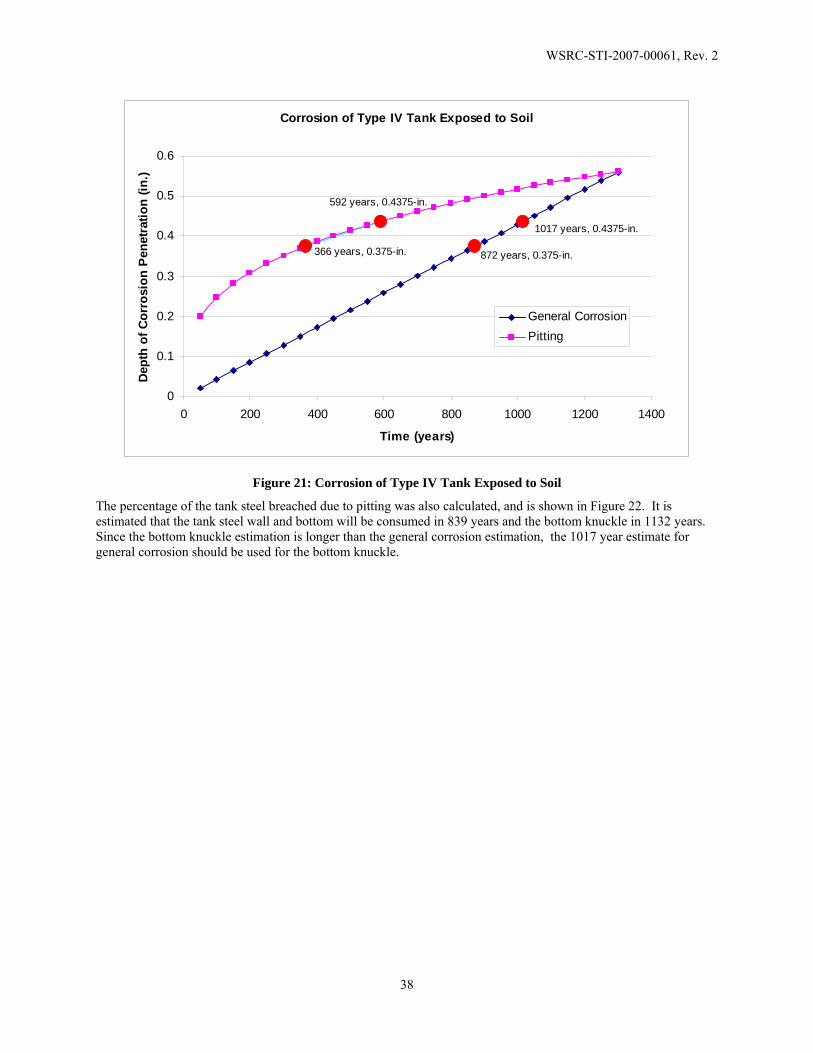
The Type IV tanks are built of 0.375-in steel for the walls and tank bottom, while the bottom knuckle is 0.4375-in. The corrosion of the Type IV tanks when exposed to soil is shown in Figure 21. The maximum pit depth and depth of general corrosion are shown as a function of time. It is estimated the first pit penetrates thru-wall at 366 years for the tank walls and bottom, and 592 years for the bottom knuckle. The general corrosion is estimated to consume the tank wall and bottom in 872 years and the bottom knuckle in 1017 years.

WSRC-STI-2007-00061, Rev. 2

38

Corrosion of Type IV Tank Exposed to Soil

872 years, 0.375-in.

1017 years, 0.4375-in.

592 years, 0.4375-in.

366 years, 0.375-in.

0

0.1

0.2

0.3

0.4

0.5

0.6

0 200 400 600 800 1000 1200 1400

Time (years)

Dep

th o

f Cor

rosi

on P

enet

ratio

n (in

.)

General CorrosionPitting

Figure 21: Corrosion of Type IV Tank Exposed to Soil

The percentage of the tank steel breached due to pitting was also calculated, and is shown in Figure 22. It is estimated that the tank steel wall and bottom will be consumed in 839 years and the bottom knuckle in 1132 years. Since the bottom knuckle estimation is longer than the general corrosion estimation, the 1017 year estimate for general corrosion should be used for the bottom knuckle.

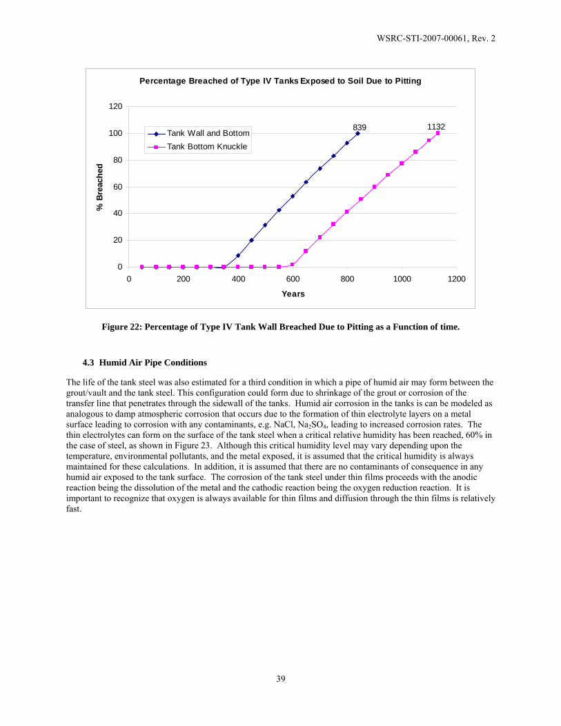
WSRC-STI-2007-00061, Rev. 2

39

Percentage Breached of Type IV Tanks Exposed to Soil Due to Pitting

839 1132

0

20

40

60

80

100

120

0 200 400 600 800 1000 1200

Years

% B

reac

hed

Tank Wall and BottomTank Bottom Knuckle

Figure 22: Percentage of Type IV Tank Wall Breached Due to Pitting as a Function of time.

4.3 Humid Air Pipe Conditions

The life of the tank steel was also estimated for a third condition in which a pipe of humid air may form between the grout/vault and the tank steel. This configuration could form due to shrinkage of the grout or corrosion of the transfer line that penetrates through the sidewall of the tanks. Humid air corrosion in the tanks is can be modeled as analogous to damp atmospheric corrosion that occurs due to the formation of thin electrolyte layers on a metal surface leading to corrosion with any contaminants, e.g. NaCl, Na2SO4, leading to increased corrosion rates. The thin electrolytes can form on the surface of the tank steel when a critical relative humidity has been reached, 60% in the case of steel, as shown in Figure 23. Although this critical humidity level may vary depending upon the temperature, environmental pollutants, and the metal exposed, it is assumed that the critical humidity is always maintained for these calculations. In addition, it is assumed that there are no contaminants of consequence in any humid air exposed to the tank surface. The corrosion of the tank steel under thin films proceeds with the anodic reaction being the dissolution of the metal and the cathodic reaction being the oxygen reduction reaction. It is important to recognize that oxygen is always available for thin films and diffusion through the thin films is relatively fast.

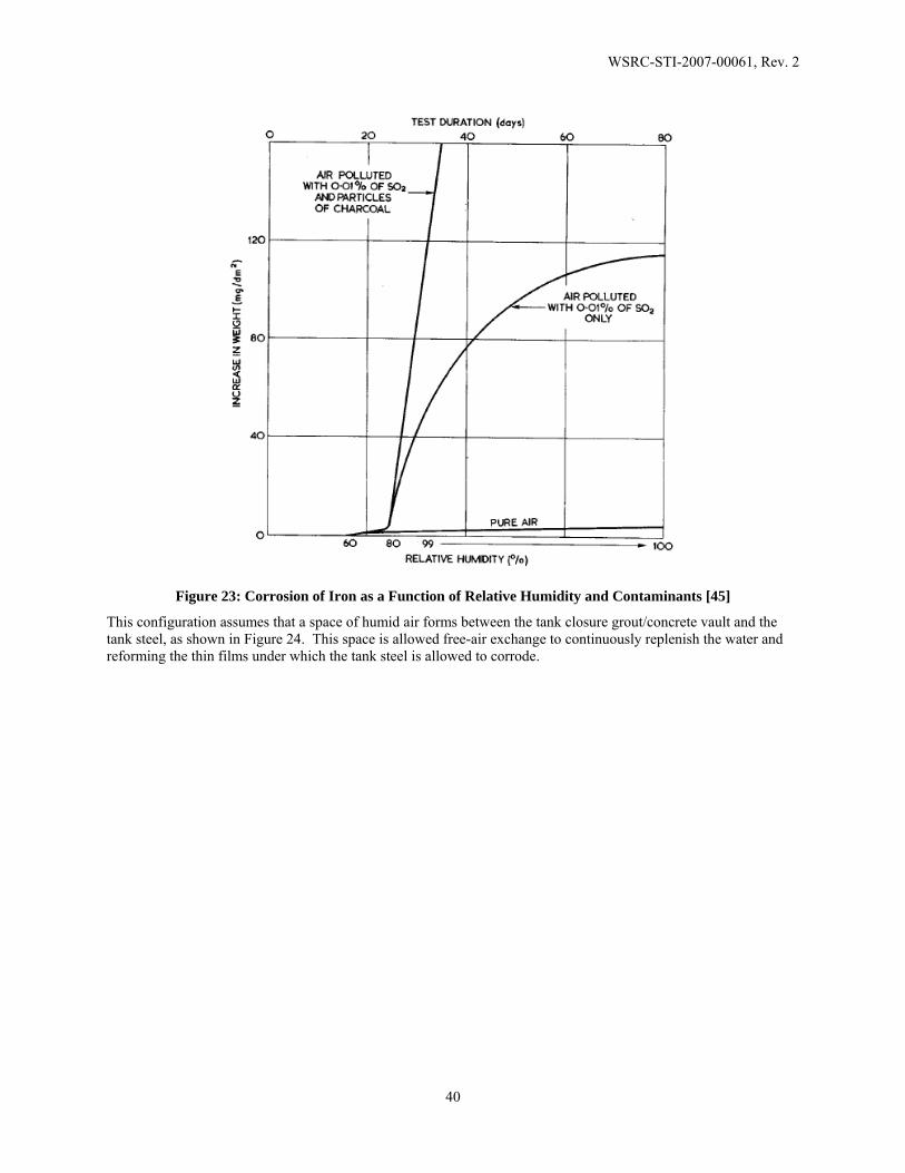
WSRC-STI-2007-00061, Rev. 2

40

Figure 23: Corrosion of Iron as a Function of Relative Humidity and Contaminants [45]

This configuration assumes that a space of humid air forms between the tank closure grout/concrete vault and the tank steel, as shown in Figure 24. This space is allowed free-air exchange to continuously replenish the water and reforming the thin films under which the tank steel is allowed to corrode.

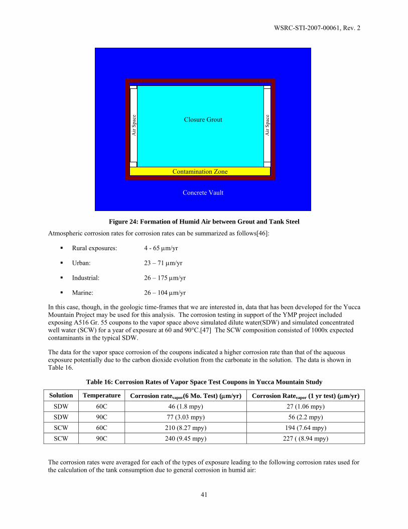
WSRC-STI-2007-00061, Rev. 2

41

Figure 24: Formation of Humid Air between Grout and Tank Steel

Atmospheric corrosion rates for corrosion rates can be summarized as follows[46]:

Rural exposures: 4 - 65 µm/yr

Urban: 23 – 71 µm/yr

Industrial: 26 – 175 µm/yr

Marine: 26 – 104 µm/yr

In this case, though, in the geologic time-frames that we are interested in, data that has been developed for the Yucca Mountain Project may be used for this analysis. The corrosion testing in support of the YMP project included exposing A516 Gr. 55 coupons to the vapor space above simulated dilute water(SDW) and simulated concentrated well water (SCW) for a year of exposure at 60 and 90°C.[47] The SCW composition consisted of 1000x expected contaminants in the typical SDW.

The data for the vapor space corrosion of the coupons indicated a higher corrosion rate than that of the aqueous exposure potentially due to the carbon dioxide evolution from the carbonate in the solution. The data is shown in Table 16.

Table 16: Corrosion Rates of Vapor Space Test Coupons in Yucca Mountain Study

Solution Temperature Corrosion ratevapor(6 Mo. Test) (µm/yr) Corrosion Ratevapor (1 yr test) (µm/yr) SDW 60C 46 (1.8 mpy) 27 (1.06 mpy) SDW 90C 77 (3.03 mpy) 56 (2.2 mpy) SCW 60C 210 (8.27 mpy) 194 (7.64 mpy) SCW 90C 240 (9.45 mpy) 227 ( (8.94 mpy)

The corrosion rates were averaged for each of the types of exposure leading to the following corrosion rates used for the calculation of the tank consumption due to general corrosion in humid air:

Contamination Zone

Concrete Vault

Closure Grout

Air

Spac

e

Air

Spac

e

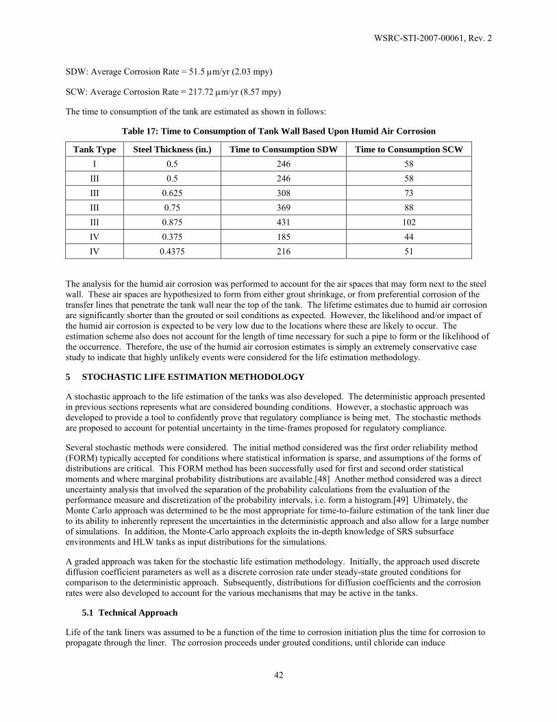
WSRC-STI-2007-00061, Rev. 2

42

SDW: Average Corrosion Rate = 51.5 µm/yr (2.03 mpy)

SCW: Average Corrosion Rate = 217.72 µm/yr (8.57 mpy)

The time to consumption of the tank are estimated as shown in follows:

Table 17: Time to Consumption of Tank Wall Based Upon Humid Air Corrosion

Tank Type Steel Thickness (in.) Time to Consumption SDW Time to Consumption SCW I 0.5 246 58

III 0.5 246 58 III 0.625 308 73 III 0.75 369 88 III 0.875 431 102 IV 0.375 185 44 IV 0.4375 216 51

The analysis for the humid air corrosion was performed to account for the air spaces that may form next to the steel wall. These air spaces are hypothesized to form from either grout shrinkage, or from preferential corrosion of the transfer lines that penetrate the tank wall near the top of the tank. The lifetime estimates due to humid air corrosion are significantly shorter than the grouted or soil conditions as expected. However, the likelihood and/or impact of the humid air corrosion is expected to be very low due to the locations where these are likely to occur. The estimation scheme also does not account for the length of time necessary for such a pipe to form or the likelihood of the occurrence. Therefore, the use of the humid air corrosion estimates is simply an extremely conservative case study to indicate that highly unlikely events were considered for the life estimation methodology.

5 STOCHASTIC LIFE ESTIMATION METHODOLOGY

A stochastic approach to the life estimation of the tanks was also developed. The deterministic approach presented in previous sections represents what are considered bounding conditions. However, a stochastic approach was developed to provide a tool to confidently prove that regulatory compliance is being met. The stochastic methods are proposed to account for potential uncertainty in the time-frames proposed for regulatory compliance.

Several stochastic methods were considered. The initial method considered was the first order reliability method (FORM) typically accepted for conditions where statistical information is sparse, and assumptions of the forms of distributions are critical. This FORM method has been successfully used for first and second order statistical moments and where marginal probability distributions are available.[48] Another method considered was a direct uncertainty analysis that involved the separation of the probability calculations from the evaluation of the performance measure and discretization of the probability intervals, i.e. form a histogram.[49] Ultimately, the Monte Carlo approach was determined to be the most appropriate for time-to-failure estimation of the tank liner due to its ability to inherently represent the uncertainties in the deterministic approach and also allow for a large number of simulations. In addition, the Monte-Carlo approach exploits the in-depth knowledge of SRS subsurface environments and HLW tanks as input distributions for the simulations.

A graded approach was taken for the stochastic life estimation methodology. Initially, the approach used discrete diffusion coefficient parameters as well as a discrete corrosion rate under steady-state grouted conditions for comparison to the deterministic approach. Subsequently, distributions for diffusion coefficients and the corrosion rates were also developed to account for the various mechanisms that may be active in the tanks.

5.1 Technical Approach

Life of the tank liners was assumed to be a function of the time to corrosion initiation plus the time for corrosion to propagate through the liner. The corrosion proceeds under grouted conditions, until chloride can induce

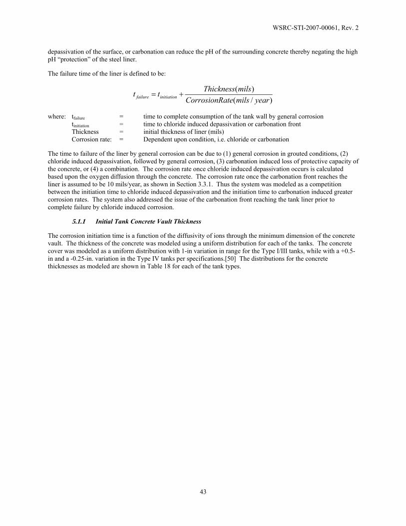
WSRC-STI-2007-00061, Rev. 2

43

depassivation of the surface, or carbonation can reduce the pH of the surrounding concrete thereby negating the high pH “protection” of the steel liner.

The failure time of the liner is defined to be:

)/()(yearmilsateCorrosionR

milsThicknesstt initiationfailure +=

where: tfailure = time to complete consumption of the tank wall by general corrosion tinitiation = time to chloride induced depassivation or carbonation front Thickness = initial thickness of liner (mils) Corrosion rate: = Dependent upon condition, i.e. chloride or carbonation

The time to failure of the liner by general corrosion can be due to (1) general corrosion in grouted conditions, (2) chloride induced depassivation, followed by general corrosion, (3) carbonation induced loss of protective capacity of the concrete, or (4) a combination. The corrosion rate once chloride induced depassivation occurs is calculated based upon the oxygen diffusion through the concrete. The corrosion rate once the carbonation front reaches the liner is assumed to be 10 mils/year, as shown in Section 3.3.1. Thus the system was modeled as a competition between the initiation time to chloride induced depassivation and the initiation time to carbonation induced greater corrosion rates. The system also addressed the issue of the carbonation front reaching the tank liner prior to complete failure by chloride induced corrosion.

5.1.1 Initial Tank Concrete Vault Thickness

The corrosion initiation time is a function of the diffusivity of ions through the minimum dimension of the concrete vault. The thickness of the concrete was modeled using a uniform distribution for each of the tanks. The concrete cover was modeled as a uniform distribution with 1-in variation in range for the Type I/III tanks, while with a +0.5-in and a -0.25-in. variation in the Type IV tanks per specifications.[50] The distributions for the concrete thicknesses as modeled are shown in Table 18 for each of the tank types.

WSRC-STI-2007-00061, Rev. 2

44

Table 18: Distributions of Tank Concrete Vault Thicknesses

Distribution of Type I Tank Concrete Thickness (in.)

Distribution of Type III Tank Concrete Thickness (in.)

Distribution of Type IV Tank Concrete Thickness (in.)

2121.221.421.621.8

2222.222.422.622.8

23

Quantiles 100.0% maximum 23.000

99.5% 22.990

97.5% 22.950

90.0% 22.799

75.0% quartile 22.499

50.0% median 21.998

25.0% quartile 21.499

10.0% 21.199

2.5% 21.050

0.5% 21.010

0.0% minimum 21.000

Moments Mean 21.999208

Std Dev 0.577186

Std Err Mean 0.0005772

upper 95% Mean 22.00034

lower 95% Mean 21.998077

N 1000000

2929.229.429.629.8

3030.230.430.630.8

31


99.5% 30.990

97.5% 30.950

90.0% 30.800

75.0% quartile 30.500

50.0% median 30.000

25.0% quartile 29.502

10.0% 29.201

2.5% 29.050

0.5% 29.010

0.0% minimum 29.000


Std Dev 0.5769515


upper 95% Mean 30.001612

lower 95% Mean 29.99935

N 1000000

3.8

3.9

4

4.1

4.2


99.5% 4.2475

97.5% 4.2375

90.0% 4.2001

75.0% quartile 4.1251

50.0% median 4.0005

25.0% quartile 3.8751

10.0% 3.7998

2.5% 3.7625

0.5% 3.7525

0.0% minimum 3.7500


Std Dev 0.1443445


upper 95% Mean 4.0004076

lower 95% Mean 3.9998418

N 1000000

5.1.2 Tank Steel Liner Thickness

The thickness of the liner was modeled using a uniform distribution per the tank steel specifications with the nominal plate thicknesses nominally as the median is shown in Table 19 each of the tank types. Steel thickness measurements made using ultrasonic techniques indicate no detectable general thinning of the waste tanks.[5]

WSRC-STI-2007-00061, Rev. 2

45

Table 19: Distribution of Tank Steel Thicknesses

Distribution of Type I Tank Steel Thickness (mils)

Distribution of Type III Tank Steel Thickness (mils)

Distribution of Type IV Tank Steel Thickness (mils)

490

500

510

520

530

Quantiles 100.0% maximum 530.00 99.5% 529.80 97.5% 529.00 90.0% 526.00 75.0% quartile 520.01 50.0% median 509.98 25.0% quartile 500.00 10.0% 494.00 2.5% 491.00 0.5% 490.20 0.0% minimum 490.00


490

500

510

520

530

Quantiles 100.0% maximum 530.0099.5% 529.8097.5% 529.0090.0% 526.0175.0% quartile 520.0450.0% median 510.0525.0% quartile 500.0310.0% 494.022.5% 491.000.5% 490.200.0% minimum 490.00


370

380

390

400

Quantiles 100.0% maximum 405.0099.5% 404.8097.5% 404.0090.0% 401.0075.0% quartile 395.0050.0% median 385.0125.0% quartile 374.9910.0% 369.002.5% 366.020.5% 365.210.0% minimum 365.00


The tank steel thicknesses may be different than the nominal thicknesses per specifications used for this analysis. Specifically, chemical cleaning utilizing oxalic acid has been proposed to remove the last remnants of waste in the tank prior to closure. An analysis of the tank closure chemical cleaning was completed to determine any major impacts on the initial thickness. Corrosion testing has been done to determine the effects of the oxalic acid cleaning process on the carbon steel. The testing recommended using the following corrosion rates for structural analyses:

Table 20: Corrosion Rates due to Oxalic Acid Chemical Cleaning Process

Corrosion Rate (mpy ±50%) Temperature (°C)

Mixed Unmixed 25 40 11 50 30 24 75 86 36

The maximum metal loss due to the cleaning process is estimated to be 7.1 mils for the following conditions:

WSRC-STI-2007-00061, Rev. 2

46

Duration of Exposure : 30 days

Temperature: 75C

Corrosion Rate: 86 mpy

5.2 Corrosion Initiation by Chloride

An empirical model, as shown in Section 3.3.2, was used to determine the chloride corrosion initiation time:

[ ] 42.0

22.1129−⋅

⋅=

ClWCRtt c

initiation

where: tinitiation = time required for initiation (years) tc = thickness of the concrete cover (in.) WCR = water-to-cement ratio [Cl-] = chloride concentration in the groundwater (ppm)

Distributions were developed for the WCR and the chloride concentration in the groundwater based upon specifications and data from SRS groundwater sampling.

5.2.1 Water to Cement Ratio Distribution

The WCR was determined to be of uniform distribution with a range of a minimum of 0.55 and a maximum of 0.65 as shown in Figure 25.

0.550.560.570.580.59

0.60.610.620.630.640.65

Figure 25: Water-to-Cement Ratio Distribution

5.2.2 Concentration of Chloride Distribution

The chloride data available from the SRS groundwater was used to develop a distribution.[28] The distribution of the chloride data is shown in Figure 26. The lognormal distribution was found to be the best fit to the data and was used for the simulations.

Quantiles of WCR 100.0% maximum 0.65000 99.5% 0.64951 97.5% 0.64746 90.0% 0.63996 75.0% quartile 0.62498 50.0% median 0.59998 25.0% quartile 0.57503 10.0% 0.56005 2.5% 0.55249 0.5% 0.55050 0.0% minimum 0.55000

Mean 0.5999918

Std Dev 0.0288494 Std Err Mean 2.8849e-5

upper 95% Mean 0.6000483 lower 95% Mean 0.5999352

N 1000000

WSRC-STI-2007-00061, Rev. 2

47

7

10

13

16

19

22

25

28

31

Figure 26:Chloride Distribution per SRS Groundwater

5.3 Corrosion by Carbonation

The initiation to carbonation was modeled using Fick’s first law as shown in Section 3.3.1. The carbonation model was approximated by:

21

2 ⎟⎟⎠

⎞⎜⎜⎝

⎛=

g

gwi CC

DX

where: X = carbonation depth (cm) (depth of the concrete vault per Section 5.1. Di = intrinsic diffusion coefficient of CO2 in concrete (cm2/s) Cgw = total inorganic carbon in ground water or soil moisture (mole/cm3)

Cg = CO2 bulk concentration in concrete solid (mole/cm3) t = time (s)

The carbonation depth was modeled as the concrete vault thickness required for the carbonation front to arrive at the steel/concrete interface thereby eliminating the high pH protection of the tank steel. The simulations for the partial stochastic were performed for the series of discrete diffusion coefficients of 1x10-8, 1x 10-6, and 1x10-4 cm2/sec.

5.3.1 Inorganic Carbon Content Distribution

The total inorganic carbon in the groundwater was modeled based upon the data from SRS groundwater measurements, as shown in Figure 27.[28]

Quantiles of [Cl-] (ppm) 100.0% maximum 31.407 99.5% 10.346 97.5% 8.874 90.0% 7.849 75.0% quartile 7.270 50.0% median 6.867 25.0% quartile 6.620 10.0% 6.480 2.5% 6.383 0.5% 6.327 0.0% minimum 6.249

Mean 7.0594733

Std Dev 0.6919333 Std Err Mean 0.0006919


N 1000000

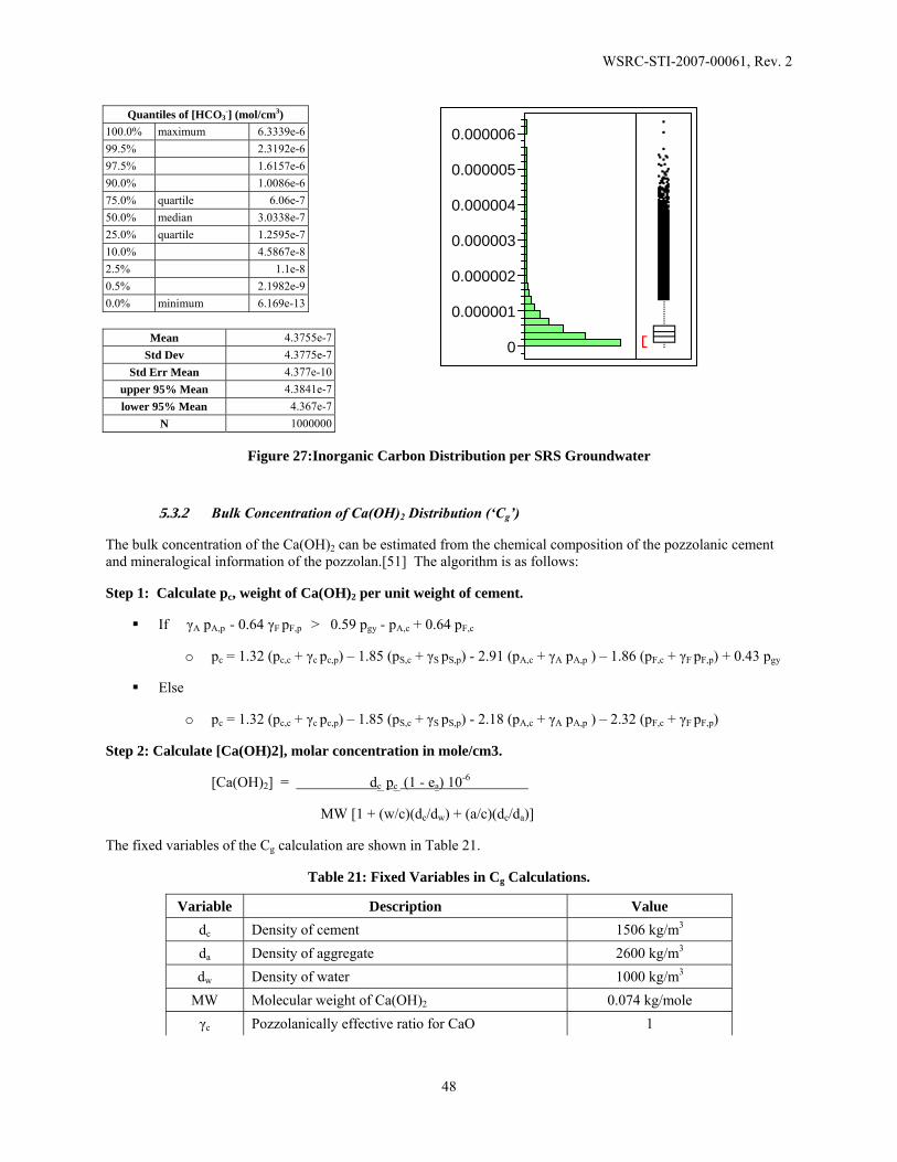
WSRC-STI-2007-00061, Rev. 2

48

0

0.000001

0.000002

0.000003

0.000004

0.000005

0.000006

Figure 27:Inorganic Carbon Distribution per SRS Groundwater

5.3.2 Bulk Concentration of Ca(OH)2 Distribution (‘Cg’)

The bulk concentration of the Ca(OH)2 can be estimated from the chemical composition of the pozzolanic cement and mineralogical information of the pozzolan.[51] The algorithm is as follows:

Step 1: Calculate pc, weight of Ca(OH)2 per unit weight of cement.

If γA pA,p - 0.64 γF pF,p > 0.59 pgy - pA,c + 0.64 pF,c

o pc = 1.32 (pc,c + γc pc,p) – 1.85 (pS,c + γS pS,p) - 2.91 (pA,c + γA pA,p ) – 1.86 (pF,c + γF pF,p) + 0.43 pgy

Else

o pc = 1.32 (pc,c + γc pc,p) – 1.85 (pS,c + γS pS,p) - 2.18 (pA,c + γA pA,p ) – 2.32 (pF,c + γF pF,p)

Step 2: Calculate [Ca(OH)2], molar concentration in mole/cm3.

[Ca(OH)2] = dc pc (1 - ea) 10-6

MW [1 + (w/c)(dc/dw) + (a/c)(dc/da)]

The fixed variables of the Cg calculation are shown in Table 21.

Table 21: Fixed Variables in Cg Calculations.

Variable Description Value dc Density of cement 1506 kg/m3 da Density of aggregate 2600 kg/m3 dw Density of water 1000 kg/m3

MW Molecular weight of Ca(OH)2 0.074 kg/mole γc Pozzolanically effective ratio for CaO 1

Quantiles of [HCO3-] (mol/cm3)

100.0% maximum 6.3339e-6 99.5% 2.3192e-6 97.5% 1.6157e-6 90.0% 1.0086e-6 75.0% quartile 6.06e-7 50.0% median 3.0338e-7 25.0% quartile 1.2595e-7 10.0% 4.5867e-8 2.5% 1.1e-8 0.5% 2.1982e-9 0.0% minimum 6.169e-13

Mean 4.3755e-7

Std Dev 4.3775e-7 Std Err Mean 4.377e-10

upper 95% Mean 4.3841e-7 lower 95% Mean 4.367e-7

N 1000000

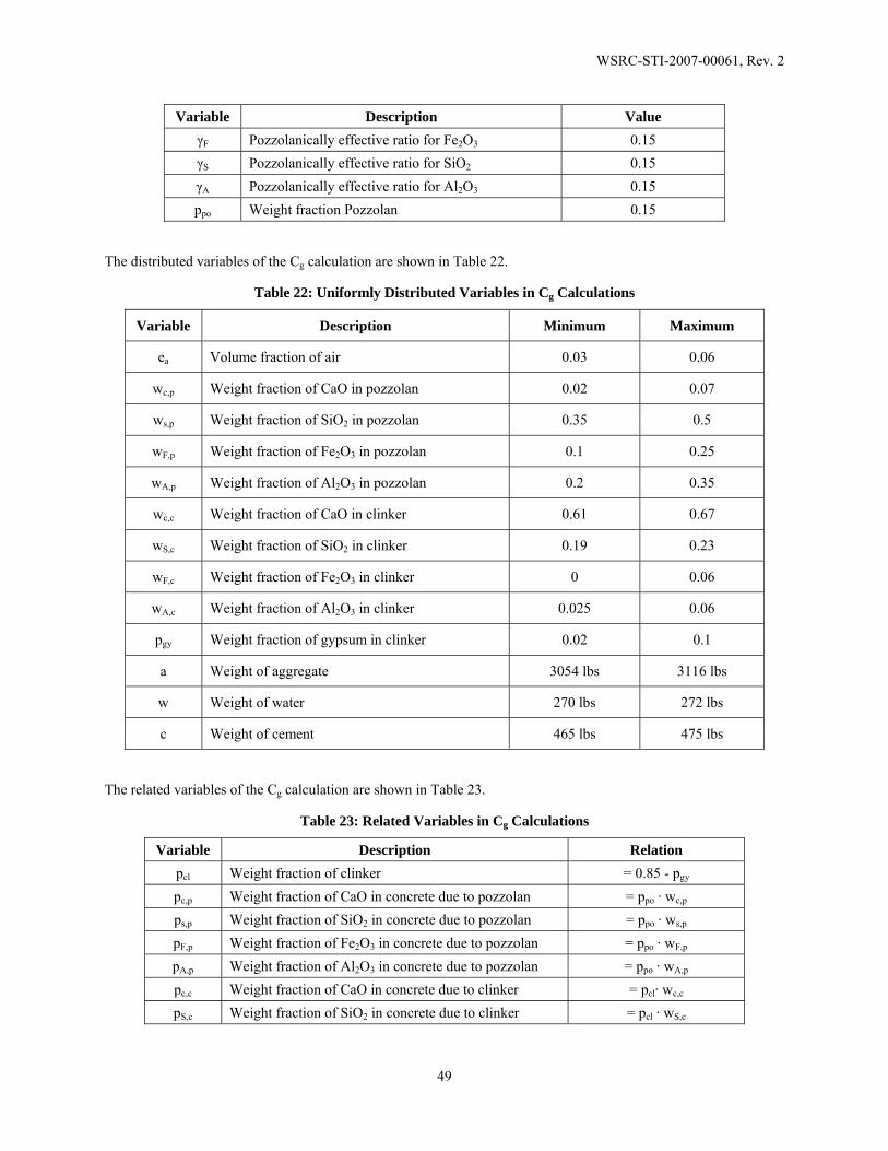
WSRC-STI-2007-00061, Rev. 2

49

Variable Description Value γF Pozzolanically effective ratio for Fe2O3 0.15 γS Pozzolanically effective ratio for SiO2 0.15 γA Pozzolanically effective ratio for Al2O3 0.15 ppo Weight fraction Pozzolan 0.15

The distributed variables of the Cg calculation are shown in Table 22.

Table 22: Uniformly Distributed Variables in Cg Calculations

Variable Description Minimum Maximum

ea Volume fraction of air 0.03 0.06

wc,p Weight fraction of CaO in pozzolan 0.02 0.07

ws,p Weight fraction of SiO2 in pozzolan 0.35 0.5

wF,p Weight fraction of Fe2O3 in pozzolan 0.1 0.25

wA,p Weight fraction of Al2O3 in pozzolan 0.2 0.35

wc,c Weight fraction of CaO in clinker 0.61 0.67

wS,c Weight fraction of SiO2 in clinker 0.19 0.23

wF,c Weight fraction of Fe2O3 in clinker 0 0.06

wA,c Weight fraction of Al2O3 in clinker 0.025 0.06

pgy Weight fraction of gypsum in clinker 0.02 0.1

a Weight of aggregate 3054 lbs 3116 lbs

w Weight of water 270 lbs 272 lbs

c Weight of cement 465 lbs 475 lbs

The related variables of the Cg calculation are shown in Table 23.

Table 23: Related Variables in Cg Calculations

Variable Description Relation pcl Weight fraction of clinker = 0.85 - pgy pc,p Weight fraction of CaO in concrete due to pozzolan = ppo · wc,p ps,p Weight fraction of SiO2 in concrete due to pozzolan = ppo · ws,p pF,p Weight fraction of Fe2O3 in concrete due to pozzolan = ppo · wF,p pA,p Weight fraction of Al2O3 in concrete due to pozzolan = ppo · wA,p pc,c Weight fraction of CaO in concrete due to clinker = pcl· wc,c pS,c Weight fraction of SiO2 in concrete due to clinker = pcl · wS,c

WSRC-STI-2007-00061, Rev. 2

50

Variable Description Relation pF,c Weight fraction of Fe2O3 in concrete due to clinker = pcl · wF,c pA,c Weight fraction of Al2O3 in concrete due to clinker = pcl · wA,c

The calculation of the bulk Ca(OH)2 resulted in the distribution shown in Figure 28. The original Cg used for the deterministic approach was 0.02 mol/cm3, whereas this more detailed analysis of chemical composition yields a median of 0.0006, which is two orders of magnitude lower, thereby decreasing the time to carbonation initiation time.

0.00020.00030.00040.00050.00060.00070.00080.00090.001

0.00110.0012

Figure 28: Bulk Ca(OH)2 (‘Cg’)Concentration Distribution

5.4 Cases of Potential Corrosion

Three specific cases were modeled per the Monte Carlo simulation: Carbonation induced corrosion was considered the most aggressive mechanism due to the high corrosion rate assumed, i.e. 10 mils/yr.

5.4.1 Case 1: IF tinitiation [Cl-] ≥ tinitiation [Carbonation]

If the time to initiation of chloride induced corrosion is greater than or equal to the time to initiation of carbonation, then carbonation was considered the controlling corrosion mechanism. Thus the time to failure was modeled as:

)/()(

][ yearmilsateCorrosionRmilsThicknesstt ncarbonatioinitiationfailure +=

where: T0 = Initial Thickness (mils) Thickness = T0 – 0.04*tinit[carbonation] [mils] Corrosion Rate (Rcarbonation) = 10 mils/year

This then yields:

Quantiles of [Ca(OH)2] (mol/cm3) 100.0% maximum 0.00122 99.5% 0.00105 97.5% 0.00097 90.0% 0.00088 75.0% quartile 0.00079 50.0% median 0.00068 25.0% quartile 0.00058 10.0% 0.00049 2.5% 0.00040 0.5% 0.00032 0.0% minimum 0.00019

Mean 0.000682



N 1000000

WSRC-STI-2007-00061, Rev. 2

51

)(10

)(04.0 ][

][

yrmils

tyr

milsTtt

ncarbonatioinitiationo

ncarbonatioinitiationfailure

⎟⎟⎠

⎞⎜⎜⎝

⎛⋅−

+=

The steel corrodes at the 0.04 mils/yr rate until the initiation of corrosion due to carbonation, followed by the increase in the corrosion rate to 10 mils/year.

5.4.2 Case 2: IF tinitiation [Cl-] < tinitiation [Carbonation]

If the initiation time to carbonation induced corrosion is greater than the initiation time to chloride induced corrosion, then the corrosion rate due to oxygen diffusion after chloride induced depassivation is calculated to determine the failure time. This was modeled as:

)/()(

][ yearmilsateCorrosionRmilsThicknesstt chlorideinitiationfailure +=

Where: T0 = Initial Thickness (mils) Thickness = T0 – 0.04*tinit[chloride] [mils] Corrosion Rate (RCl-) = Calculated

The corrosion rate is calculated, as shown in Section 3.3.2, by:

Fe

FeOcorrosion

MNRρ23

4=

where: MFe = molecular weight of iron (56 g/mol) ρFe = density of iron (7.86 g/cm3)

The oxygen diffusion through the concrete is represented by:

XC

DN gwiO ∆

=2

where: NO2 = flux of oxygen through concrete (mol/s/cm2) Di = oxygen diffusion coefficient in concrete (cm2/sec)

Cgw = concentration of oxygen in groundwater (mol/cm3) ∆X = Depth of concrete (cm)

The corrosion rate simulations were performed for the series of discrete oxygen diffusion coefficients of 1x10-8, 1x 10-6, and 1x10-4 cm2/sec for each, Type I, III, and IV tanks. The results, shown in Table 24 - 26, conclude that corrosion rates were primarily below the 0.04 mils/year, which was used as the minimum acceptable corrosion rate for failure estimations. The corrosion rates for the 1x10e-6 and 1x10-8 diffusion coefficients were lower than 0.04 mils/year for all types of tanks.

WSRC-STI-2007-00061, Rev. 2

52

Table 24: Calculated Corrosion Rate after Chloride Induced Depassivation for Type I Tanks

RCl : Di(O2)=0.0001 RCl : Di(O2)=0.000001 RCl : Di(O2)=0.00000001

00.010.020.030.040.050.060.070.080.090.1

Quantiles

100.0% maximum 0.10242 99.5% 0.07649 97.5% 0.07042 90.0% 0.06353 75.0% quartile 0.05690 50.0% median 0.04754 25.0% quartile 0.01181 10.0% 0.00066 2.5% 0.00017 0.5% 3.31e-5 0.0% minimum 6.18e-9




N 1000000

00.00010.00020.00030.00040.00050.00060.00070.00080.00090.001

Quantiles

100.0% maximum 0.0010299.5% 0.0007697.5% 0.0007090.0% 0.0006475.0% quartile 0.0005750.0% median 0.0004825.0% quartile 0.0001210.0% 6.6e-6 2.5% 1.66e-6 0.5% 3.31e-7 0.0% minimum 6.2e-11


Std Dev 0.0002414Std Err Mean 2.4137e-7

upper 95% Mean 0.0003801lower 95% Mean 0.0003791

N 1000000

00.0000010.0000020.0000030.0000040.0000050.0000060.0000070.0000080.0000090.00001

Quantiles

100.0% maximum 0.0000199.5% 7.65e-6 97.5% 7.04e-6 90.0% 6.35e-6 75.0% quartile 5.69e-6 50.0% median 4.75e-6 25.0% quartile 1.18e-6 10.0% 6.6e-8 2.5% 1.66e-8 0.5% 3.31e-9 0.0% minimum 6.2e-13

Moments Mean 3.7962e-6

Std Dev 2.4137e-6 Std Err Mean 2.4137e-9

upper 95% Mean 0.0000038lower 95% Mean 3.7914e-6

N 1000000

WSRC-STI-2007-00061, Rev. 2

53

Table 25: Calculated Corrosion Rate after Chloride Induced Depassivation for Type III Tanks


0

0.01

0.02

0.03

0.04

0.05

0.06

0.07

Quantiles

100.0% maximum 0.07375 99.5% 0.05592 97.5% 0.05152 90.0% 0.04654 75.0% quartile 0.04171 50.0% median 0.03488 25.0% quartile 0.00866 10.0% 0.00048 2.5% 0.00012 0.5% 2.43e-5 0.0% minimum 4.36e-9

Moments

Mean 0.0278297 Std Dev 0.0176845 Std Err Mean 1.7684e-5 upper 95% Mean 0.0278643 lower 95% Mean 0.027795 N 1000000

0

0.0001

0.0002

0.0003

0.0004

0.0005

0.0006

0.0007

Quantiles

100.0% maximum 0.0007499.5% 0.0005697.5% 0.0005290.0% 0.0004775.0% quartile 0.0004250.0% median 0.0003525.0% quartile 8.66e-510.0% 4.84e-62.5% 1.22e-60.5% 2.43e-70.0% minimum 4.4e-11

Moments

Mean 0.0002783Std Dev 0.0001768Std Err Mean 1.7684e-7upper 95% Mean 0.0002786lower 95% Mean 0.000278N 1000000

0

0.000001

0.000002

0.000003

0.000004

0.000005

0.000006

0.000007

Quantiles 100.0% maximum 7.3749e-699.5% 5.592e-697.5% 5.1523e-690.0% 4.6539e-675.0% quartile 4.1713e-650.0% median 3.4882e-625.0% quartile 8.6633e-710.0% 4.8355e-82.5% 1.2177e-80.5% 2.4261e-90.0% minimum 4.359e-13

Moments

Mean 2.783e-6Std Dev 1.7684e-6Std Err Mean 1.7684e-9upper 95% Mean 2.7864e-6lower 95% Mean 2.7795e-6N 1000000

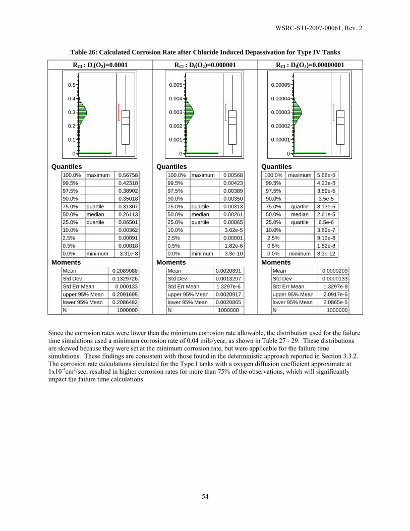
WSRC-STI-2007-00061, Rev. 2

54

Table 26: Calculated Corrosion Rate after Chloride Induced Depassivation for Type IV Tanks


0

0.1

0.2

0.3

0.4

0.5

Quantiles

100.0% maximum 0.56758 99.5% 0.42318 97.5% 0.38902 90.0% 0.35018 75.0% quartile 0.31307 50.0% median 0.26113 25.0% quartile 0.06501 10.0% 0.00362 2.5% 0.00091 0.5% 0.00018 0.0% minimum 3.31e-8


0

0.001

0.002

0.003

0.004

0.005

Quantiles

100.0% maximum 0.0056899.5% 0.0042397.5% 0.0038990.0% 0.0035075.0% quartile 0.0031350.0% median 0.0026125.0% quartile 0.0006510.0% 3.62e-52.5% 0.000010.5% 1.82e-60.0% minimum 3.3e-10

Moments Mean 0.0020891Std Dev 0.0013297Std Err Mean 1.3297e-6 upper 95% Mean 0.0020917lower 95% Mean 0.0020865N 1000000

0

0.00001

0.00002

0.00003

0.00004

0.00005

Quantiles

100.0% maximum 5.68e-599.5% 4.23e-597.5% 3.89e-590.0% 3.5e-5 75.0% quartile 3.13e-550.0% median 2.61e-525.0% quartile 6.5e-6 10.0% 3.62e-72.5% 9.12e-80.5% 1.82e-80.0% minimum 3.3e-12

Moments Mean 0.0000209Std Dev 0.0000133Std Err Mean 1.3297e-8upper 95% Mean 2.0917e-5lower 95% Mean 2.0865e-5N 1000000

Since the corrosion rates were lower than the minimum corrosion rate allowable, the distribution used for the failure time simulations used a minimum corrosion rate of 0.04 mils/year, as shown in Table 27 - 29. These distributions are skewed because they were set at the minimum corrosion rate, but were applicable for the failure time simulations. These findings are consistent with those found in the deterministic approach reported in Section 3.3.2. The corrosion rate calculations simulated for the Type I tanks with a oxygen diffusion coefficient approximate at 1x10-4cm2/sec, resulted in higher corrosion rates for more than 75% of the observations, which will significantly impact the failure time calculations.

WSRC-STI-2007-00061, Rev. 2

55

Table 27: Corrosion Rate used for Simulations after Chloride Induced Depassivation for Type I Tanks


0.04

0.05

0.06

0.07

0.08

0.09

0.1

Quantiles

100.0% maximum 0.10469 99.5% 0.07641 97.5% 0.07042 90.0% 0.06352 75.0% quartile 0.05689 50.0% median 0.04754 25.0% quartile 0.04000 10.0% 0.04000 2.5% 0.04000 0.5% 0.04000 0.0% minimum 0.04000

Moments Mean 0.0494059 Std Dev 0.0098131 Std Err Mean 9.8131e-6 upper 95% Mean 0.0494251 lower 95% Mean 0.0493867 N 1000000

0.040.0410.0420.0430.0440.0450.0460.0470.0480.0490.05

Quantiles

100.0% maximum 0.0400099.5% 0.0400097.5% 0.0400090.0% 0.0400075.0% quartile 0.0400050.0% median 0.0400025.0% quartile 0.0400010.0% 0.040002.5% 0.040000.5% 0.040000.0% minimum 0.04000

Moments Mean 0.04Std Dev 0Std Err Mean 0upper 95% Mean 0.04lower 95% Mean 0.04N 1000000

0.040.0410.0420.0430.0440.0450.0460.0470.0480.0490.05

Quantiles



WSRC-STI-2007-00061, Rev. 2

56

Table 28: Corrosion Rate used for Simulations after Chloride Induced Depassivation for Type III Tanks


0.04

0.05

0.06

0.07

Quantiles


Moments Mean 0.041646 Std Dev 0.0032946 Std Err Mean 3.2946e-6 upper 95% Mean 0.0416524 lower 95% Mean 0.0416395 N 1000000

0.040.0410.0420.0430.0440.0450.0460.0470.0480.0490.05

Quantiles



0.040.0410.0420.0430.0440.0450.0460.0470.0480.0490.05

Quantiles



WSRC-STI-2007-00061, Rev. 2

57

Table 29: Corrosion Rate used for Simulations after Chloride Induced Depassivation for Type IV Tanks


0.1

0.2

0.3

0.4

0.5

Quantiles


Moments Mean 0.2166468 Std Dev 0.1213474 Std Err Mean 1e-4213 upper 95% Mean 0.2168847 lower 95% Mean 0.216409 N 1000000

0.040.0410.0420.0430.0440.0450.0460.0470.0480.0490.05

Quantiles



0.040.0410.0420.0430.0440.0450.0460.0470.0480.0490.05

Quantiles



5.4.3 Case 3: IF tfailure [Cl-] ≥ tinitiation [Carbonation]

The third case for failure of the steel liner due to corrosion is if the carbonation front reaches the steel liner prior to the failure of the steel line due to chloride. This is particularly critical, because the corrosion rates subsequent to chloride induced depassivation are equivalent to the minimum in the majority of cases, as opposed to the corrosion rate due to carbonation, i.e. 0.04 mils/year vs. 10 mils/year.

In this case, the failure time was modeled as failure due to carbonation:

)/()(

][ yearmilsateCorrosionRmilsThicknesstt ncarbonatioinitiationfailure +=

Where the thickness of the steel liner is calculated subsequent to corrosion after the chloride induced depassivation when the carbonation front reaches:

( ) ( )[ ]04.0][][][ ⋅+⋅−− ClinitiationClClinitiationncarbonatioinitiationo tRttT

WSRC-STI-2007-00061, Rev. 2

58

Then, the failure time can be calculated as :

( ) ( )[ ])/(10

)(04.0][][][][ yearmils

milstRttTtt ClinitiationClClinitiationncarbonatioinitiationo

ncarbonatioinitiationfailure

⋅+⋅−−+=

This model accounts for the corrosion prior to chloride induced depassivation, the corrosion between the initiation time to carbonation and initiation time of chloride induced corrosion, and finally the corrosion due to carbonation.

6 RESULTS OF PARTIAL STOCHASTIC APPROACH

The Monte Carlo simulations to determine the failure times were done for various diffusion coefficients of CO2, and oxygen through the concrete vault.. The simulations were performed under the assumptions that corrosion initiates on one surface of the liner and travels through until the liner is “consumed” due to general corrosion. The results are presented as a function of tank type and diffusion coefficient combinations in the following sections.

6.1 Type I Tank : Di(CO2) = 1x10-8cm2/sec, Varied Di (O2)

The results for the simulation performed for the Type I tank where the diffusion coefficient Di(CO2) = 1x 10-8 cm2/sec is shown in Table 30. The results for Di (O2)= 1x10-4 cm2/sec diffusion rate diverge from the other results due to the increased corrosion rate from the high oxygen diffusivity. The distribution for this case clearly shows two regions. One regions appears to exhibit uniform distribution as expected from the corrosion rate due to chloride calculations, whereas a normal distribution is evident where the corrosion rates are equal to 0.04 mils/year. The corrosion rate due to chloride induced depassivation does not increase from the minimum value of 0.04 mils/year for the lower diffusion rates. In addition, the results indicate that the carbonation front does not reach the steel liner prior to failure by chloride induced corrosion.

WSRC-STI-2007-00061, Rev. 2

59

Table 30: Time to Failure for Type I Tank where Di(CO2) = 1x10-8cm2/sec, Varied Di (O2)

Time to Failure: Di(O2)=0.0001 Time to Failure: Di(O2)=0.000001 Time to Failure: Di(O2)=0.00000001

8000

9000

10000

11000

12000

13000

-5 -4 -3 -2 -1 0 1 2 3 4 5

Normal Quantile Plot



12300124001250012600127001280012900130001310013200

-5 -4 -3 -2 -1 0 1 2 3 4 5




12300124001250012600127001280012900130001310013200

-5 -4 -3 -2 -1 0 1 2 3 4 5





The results for the simulation performed for the Type I tank where the diffusion coefficient Di(CO2) = 1x 10-6 cm2/sec is shown in Table 31. The results are very similar those performed Di(CO2) = 1x 10-8 cm2/sec. The results for Di (O2)= 1x10-4 cm2/sec diffusion rate diverge from the other results due to the increased corrosion rate from the high oxygen diffusivity. The distribution for this case once again clearly shows two regions. One regions appears to exhibit uniform distribution as expected from the corrosion rate due to chloride calculations, whereas a normal distribution is evident where the corrosion rates are equal to 0.04 mils/year. The corrosion rate due to chloride induced depassivation does not increase from the minimum value of 0.04 mils/year for the lower diffusion rates. In addition, the results indicates that the carbonation front does not reach the steel liner prior to failure by chloride induced corrosion.

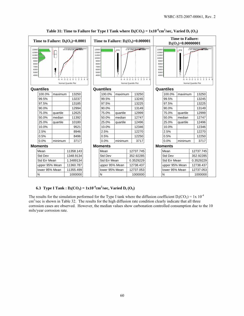
WSRC-STI-2007-00061, Rev. 2

60



400050006000700080009000

10000110001200013000

-5 -4 -3 -2 -1 0 1 2 3 4 5




400050006000700080009000

10000110001200013000

-5 -4 -3 -2 -1 0 1 2 3 4 5




400050006000700080009000

10000110001200013000

-5 -4 -3 -2 -1 0 1 2 3 4 5





The results for the simulation performed for the Type I tank where the diffusion coefficient Di(CO2) = 1x 10-4 cm2/sec is shown in Table 32. The results for the high diffusion rate condition clearly indicate that all three corrosion cases are observed. However, the median values show carbonation controlled consumption due to the 10 mils/year corrosion rate.

WSRC-STI-2007-00061, Rev. 2

61



0

2000

4000

6000

8000

10000

12000

-5 -4 -3 -2 -1 0 1 2 3 4 5




0

2000

4000

6000

8000

10000

12000

-5 -4 -3 -2 -1 0 1 2 3 4 5


Quantiles 100.0% maximum 1325099.5% 1316297.5% 1282590.0% 7367 75.0% quartile 2707 50.0% median 1140 25.0% quartile 586 10.0% 364 2.5% 238 0.5% 175 0.0% minimum 86


0

2000

4000

6000

8000

10000

12000

-5 -4 -3 -2 -1 0 1 2 3 4 5




6.4 Type III Tank : Di(CO2) = 1x10-8cm2/sec, Varied Di (O2)

The results for the simulation performed for the Type III tanks where the diffusion coefficient Di(CO2) = 1x 10-8 cm2/sec is shown in Table 33. The results for Di (O2)= 1x10-4 cm2/sec diffusion rate diverge from the other results due to the increased corrosion rate from the high oxygen diffusivity. However, the corrosion rate increase from chloride depassivation increase from the minimum was minimal and did not impact the median final time to failure but did decrease the lower bounds.

WSRC-STI-2007-00061, Rev. 2

62

Table 33: Time to Failure for Type III Tank where Di(CO2) = 1x10-8cm2/sec, Varied Di (O2)


10000

11000

12000

13000

-5 -4 -3 -2 -1 0 1 2 3 4 5




12300124001250012600127001280012900130001310013200

-5 -4 -3 -2 -1 0 1 2 3 4 5




12300124001250012600127001280012900130001310013200

-5 -4 -3 -2 -1 0 1 2 3 4 5





The results for the simulation performed for the Type III tanks where the diffusion coefficient Di(CO2) = 1x 10-6 cm2/sec is shown in Table 34. The results for Di (O2)= 1x10-4 cm2/sec diffusion rate diverge from the other results due to the increased corrosion rate from the high oxygen diffusivity. However, the corrosion rate increase from chloride depassivation increase from the minimum was minimal and did not impact the median final time to failure but did decrease the lower bounds.

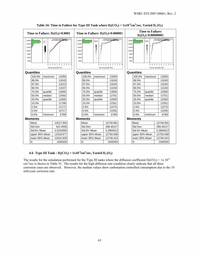
WSRC-STI-2007-00061, Rev. 2

63



7000

8000

9000

10000

11000

12000

13000

-5 -4 -3 -2 -1 0 1 2 3 4 5




7000

8000

9000

10000

11000

12000

13000

-5 -4 -3 -2 -1 0 1 2 3 4 5




7000

8000

9000

10000

11000

12000

13000

-5 -4 -3 -2 -1 0 1 2 3 4 5





The results for the simulation performed for the Type III tanks where the diffusion coefficient Di(CO2) = 1x 10-4 cm2/sec is shown in Table 35. The results for the high diffusion rate condition clearly indicate that all three corrosion cases are observed . However, the median values show carbonation controlled consumption due to the 10 mils/year corrosion rate.

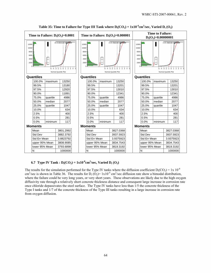
WSRC-STI-2007-00061, Rev. 2

64



0

2000

4000

6000

8000

10000

12000

-5 -4 -3 -2 -1 0 1 2 3 4 5




0

2000

4000

6000

8000

10000

12000

-5 -4 -3 -2 -1 0 1 2 3 4 5




0

2000

4000

6000

8000

10000

12000

-5 -4 -3 -2 -1 0 1 2 3 4 5




6.7 Type IV Tank : Di(CO2) = 1x10-8cm2/sec, Varied Di (O2)

The results for the simulation performed for the Type IV tanks where the diffusion coefficient Di(CO2) = 1x 10-8 cm2/sec is shown in Table 36. The results for Di (O2)= 1x10-4 cm2/sec diffusion rate show a bimodal distribution, where the failure could be very long years, or very short years. These observations are likely due to the high oxygen diffusivity rate through a relatively short concrete thickness distance and consequent large increase in corrosion rate once chloride depassivates the steel surface. The Type IV tanks have less than 1/5 the concrete thickness of the Type I tanks and 1/7 of the concrete thickness of the Type III tanks resulting in a large increase in corrosion rate from oxygen diffusion.

WSRC-STI-2007-00061, Rev. 2

65

Table 36: Time to Failure for Type IV Tank where Di(CO2) = 1x10-8cm2/sec, Varied Di (O2)


10002000

30004000

500060007000

80009000

10000

-5 -4 -3 -2 -1 0 1 2 3 4 5


Quantiles 100.0% maximum 10125

99.5% 10103

97.5% 10014

90.0% 9689

75.0% quartile 6133

50.0% median 1920

25.0% quartile 1678

10.0% 1545

2.5% 1431

0.5% 1346

0.0% minimum 1110


Std Dev 3301.6607


upper 95% Mean 3895.8665

lower 95% Mean 3882.9242

N 1000000

910092009300940095009600970098009900

1000010100

-5 -4 -3 -2 -1 0 1 2 3 4 5



99.5% 10120

97.5% 10100

90.0% 10025

75.0% quartile 9875

50.0% median 9626

25.0% quartile 9376

10.0% 9225

2.5% 9150

0.5% 9130

0.0% minimum 9125


Std Dev 288.30203


upper 95% Mean 9626.1464

lower 95% Mean 9625.0163

N 1000000

910092009300940095009600970098009900

1000010100

-5 -4 -3 -2 -1 0 1 2 3 4 5



99.5% 10120

97.5% 10100

90.0% 10025

75.0% quartile 9875

50.0% median 9626

25.0% quartile 9376

10.0% 9225

2.5% 9150

0.5% 9130

0.0% minimum 9125


Std Dev 288.30203


upper 95% Mean 9626.1464

lower 95% Mean 9625.0163

N 1000000


The results for the simulation performed for the Type IV tanks where the diffusion coefficient Di(CO2) = 1x 10-6 cm2/sec is shown in Table 37. The results for Di (O2)= 1x10-4 cm2/sec diffusion rate show a distribution indicative of carbonation as the primary mechanism of failure, and possibly initiating prior to chloride depassivation or soon thereafter. The results for Di (O2)= 1x10-6 cm2/sec and Di (O2)= 1x10-8 cm2/sec diffusion rate show a bimodal distribution, where the failure could be very long years, or very short years. The observations that are of long time frames are indicative of the corrosion rate being set at the minimum, while the corrosion rate is known to be higher due to the relatively thin concrete section.

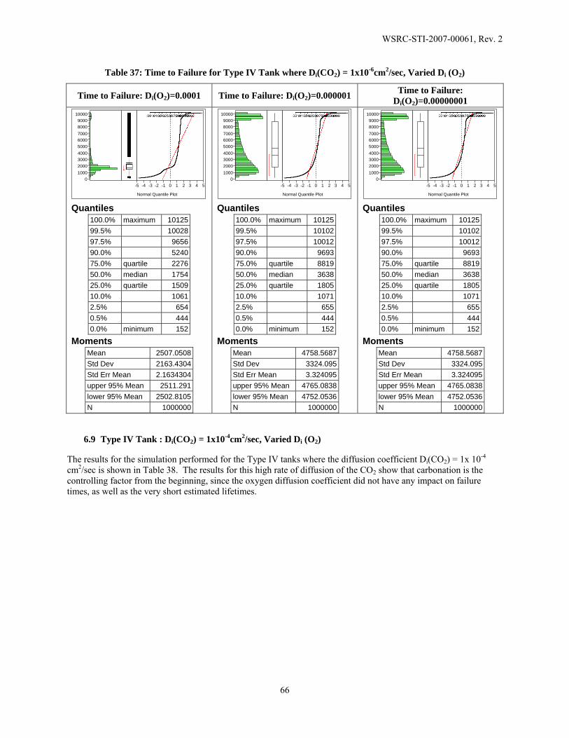
WSRC-STI-2007-00061, Rev. 2

66



0100020003000400050006000700080009000

10000

-5 -4 -3 -2 -1 0 1 2 3 4 5




0100020003000400050006000700080009000

10000

-5 -4 -3 -2 -1 0 1 2 3 4 5




0100020003000400050006000700080009000

10000

-5 -4 -3 -2 -1 0 1 2 3 4 5





The results for the simulation performed for the Type IV tanks where the diffusion coefficient Di(CO2) = 1x 10-4 cm2/sec is shown in Table 38. The results for this high rate of diffusion of the CO2 show that carbonation is the controlling factor from the beginning, since the oxygen diffusion coefficient did not have any impact on failure times, as well as the very short estimated lifetimes.

WSRC-STI-2007-00061, Rev. 2

67



0100020003000400050006000700080009000

10000

-5 -4 -3 -2 -1 0 1 2 3 4 5




0100020003000400050006000700080009000

10000

-5 -4 -3 -2 -1 0 1 2 3 4 5




0100020003000400050006000700080009000

10000

-5 -4 -3 -2 -1 0 1 2 3 4 5




7 COMPREHENSIVE STOCHASTIC METHODOLOGY

A comprehensive stochastic methodology (CSM) was also utilized to estimate the life of the tank steel liner. The comprehensive methodology developed distributions for the corrosion rate as well as the diffusion coefficients for carbon dioxide related to the potential carbonation and the oxygen related to the chloride induced depassivation of the steel.

7.1 Corrosion Rate Distribution

It was determined that use of a corrosion rate distribution is applicable to address the variability in the corrosion rates in the passive state of steel in contact with concrete as well as other conditions that may contribute to localized general corrosion, e.g. galvanic, albeit with a lower probability. It is a practical assumption that the corrosion of the carbon steel will be variant across the steel/concrete interface when these conditions are taken into account. Several conditions were taken into account in the development of the distribution used for the corrosion rate, shown in Figure 29.

WSRC-STI-2007-00061, Rev. 2

68

0

0.1

0.2

0.3

0.4

0.5

Figure 29: Distribution of Corrosion Rates

Firstly, the corrosion rate of steel in contact with the concrete vault, assumed to be quality concrete, is expected to be in a “passive” state. Passivity is the state exhibited by the metal in which corrosion is limited by the diffusion of reactants through a tenacious oxide film. However, the “passive current densities” that are indicative of a steady state corrosion rate will vary depending on the specific conditions including localized conditions on the tank surface. Although the steady state corrosion rate is largely disregarded for operational conditions, it must be addressed for the geologic time-frames that are of interest for performance assessment calculations. The passive current density can be calculated utilizing Faraday’s Law which relates the corrosion rate to the current density dependent upon the material:

EWiKCR cor

ρ1=

Where: CR = corrosion rate (mpy) K1 = 0.1288 (mpy·g/µA·cm) icor = current density (µA/cm2) r = density (g/cm3) EW = equivalent weight (atomic weight/valence)

The corresponding passive current densities for the distribution of the corrosion rates are shown in Table 39. The passive current densities vary from 0.02 µA/cm2 to 1 µA/cm2 with the broad majority in the range between 0.04 ~ 0.2 µA/cm2. These values are consistent with literature data, of which the primary sources contends a passive current density of near 0.01 µA/cm2 for buried steel/concrete structures.[24] However, there are various passive current densities reported depending upon the specific concentration of the pore water tested from 0.01 – 10 µA/cm2.[18,52] The relevant passive current density used for input into the PA are those for buried steel/concrete structures. In addition, these passive current densities and the electochemical potential regimes in which corrosion can occur is reported to be exacerbated by the presence of the chloride ion, but the SRS chloride concentrations are significantly lower than those in the literature, thereby indicating a consistent passive current density.[32] The minimum passive current density used for the calculation is twice the reported values for buried structures.

Table 39: Corresponding Passive Current Densities for Corrosion Rate Distribution

Quantiles CR (MPY) I corr (µA/cm2) 100.0% 0.44978 0.983086 99.5% 0.23641 0.516722 97.5% 0.15527 0.339374 90.0% 0.09727 0.212603

Quantiles of Corrosion Rates (mpy) 100.0% maximum 0.44978 99.5% 0.23641 97.5% .15527 90.0% 0.09727 75.0% quartile 0.06418 50.0% median 0.04058 25.0% quartile 0.02590 10.0% 0.01769 2.5% 0.01253 0.5% 0.01059 0.0% minimum 0.01

WSRC-STI-2007-00061, Rev. 2

69

Quantiles CR (MPY) I corr (µA/cm2) 75.0% 0.06418 0.140278 50.0% 0.04058 0.088696 25.0% 0.0259 0.05661 10.0% 0.01769 0.038665 2.5% 0.01253 0.027387 0.5% 0.01059 0.023147 0.0% 0.01 0.021857

The distribution of the corrosion rates is assumed to account for some of the localized areas within the tank surface that may be subject to greater than the median corrosion rate of 0.04 mpy. For example, there are locations within the tank where pumps anchored to the carbon steel bottom with stainless steel anchors will be grouted in place which may lead to galvanic corrosion currents in the slight areas of contact. The galvanic corrosion currents between stainless steel and carbon steel are known to be negligible in experimental time-frames, but were considered for this analysis due to the time-frames involved. The current density contributions from the galvanic currents particularly for a passive carbon steel are reported to stablize near 0.2 µA/cm2.[53] The area which the stainless steel contacts the carbon steel is a minute fraction of the entire surface of the tank bottom. The tank bottom surface area for the Type III tanks as an example is estimated at 11000 ft2, whereas the total area of potential contact may be less than 1 ft2. Another potential area of higher than nominal passive current densities is the welded regions of the bottom plate. Once again, the welded areas and the subsequent heat-affected zones of those welds where microstructural features may lead to greater than nominal corrosion is small in comparison to the total surface area of the nominal base metal exposed. As such, the distribution of corrosion rates is expected to encompass these regions appropriately.

The implication of the potential for a high corrosion rate to be chosen during the simulation is the occurrence of premature corrosion prior to the initiation of carbonation or chloride induced depassivation. As such, a “Case 0” was calculated as:

0 / (0.04)ft T Rnd=

where: tf = time to failure (years) T0 = Initial thickness (mils)

Rnd (0.04) = Corrosion rate chosen from distribution

when the tank fails due to general corrosion before the initiation of either corrosion mechanism. The time to failure is then used as input to determine the interaction with Cases 1-3 as presented before. It is expected that the thicker sections of concrete may fail via this mode since the time required for carbonation/chloride to reach the steel/concrete interface will be longer than the initial corrosion rate. When this is not the case, one of the initial cases will apply.

7.2 Distribution of Carbon Dioxide/Oxygen Diffusion Coefficients

The initial stochastic analysis performed Monte Carlo simulations for discrete values of carbon dioxide and oxygen diffusion rates due to the uncertainty in the diffusion coefficients of these gases through the concrete structure. However, the subsequent comprehensive analysis presented in this section developed distributions for these diffusion coefficients as input into the corrosion calculations. The distribution for the diffusion rates accounts for various scenarios that are envisioned through the concrete structure. It is assumed that the concrete structure has some distribution of solid and pore space, which may include cracks or construction joints. The diffusion rate is primarily assumed to be in the aqueous phase or the saturated phase of the concrete, and therefore the majority of the diffusion rate distribution falls in this region. In addition, there is a small probability that the pore spaces may be

WSRC-STI-2007-00061, Rev. 2

70

serially connected thereby leading to a preferential pathway allowing for complete vapor space diffusion mechanisms. The accurate determination of diffusion coefficients for mass transport through these mediums is a complex proposition and has mutliple variables affecting the output. It is typically accepted that cracking can control the mass transport through concrete structures, however, in this case, the simple thickness of the concrete structure as well as inspection knowledge of the tanks has revealed minor, if any, cracking of the concrete vault.[54] Based upon these considerations, the distribution shown in Figure 30 was developed for the diffusion coefficients of carbon dioxide as well as oxygen.

0e+01e-22e-23e-24e-25e-26e-27e-28e-29e-21e-1

Figure 30:Distribution of Diffusion Coefficients

The distribution is better represented by the logarithm of the diffusion coefficient as shown in Figure 31

-10

-9

-8

-7

-6-5

-4

-3

-2

-1

Figure 31:Distribution of the Logarithm of Diffusion Coefficients

The distribution is assumed to account for the various modes of diffusion possible, such as through a variety of pores, solids, and aqueous phase transport. The broad majority of the diffusion coefficients fall within 1x10-9

cm2/sec and 1x10-2 cm2/sec, which is expected to encompass the majority of the regions of interest. However the

Quantiles of Diffusion Coefficients 100.0% maximum 0.10000 99.5% 0.07509 97.5% 0.02822 90.0% 0.00215 75.0% quartile 0.00008 50.0% median 1.47e-6 25.0% quartile 3.06e-8 10.0% 1.68e-9 2.5% 2.3e-10 0.5% 1.2e-10 0.0% minimum 1e-10

Mean 0.0021522



N 1233023

Quantiles of Diffusion Coefficients 100.0% maximum -1.00 99.5% -1.12 97.5% -1.55 90.0% -2.67 75.0% quartile -4.09 50.0% median -5.83 25.0% quartile -7.51 10.0% -8.78 2.5% -9.63 0.5% -9.92 0.0% minimum -10.00

Mean -5.771115

Std Dev 2.2218854 Std Err Mean 0.0020009

upper 95% Mean -5.767193 lower 95% Mean -5.775037

N 1233023

WSRC-STI-2007-00061, Rev. 2

71

diffusion coefficients outside that regime are given lower probabilities with the higher diffusion coefficients accounting for preferential pathways and the lower coefficients accounting for diffusion through solid materials.

8 RESULTS OF COMPREHENSIVE STOCHASTIC ANALYSIS

The results for the CSM are presented in the following sections for the Type I/III/IIIA/IV tanks respectively. The results are presented as quantiles, log-time to failure, and the cumulative distribution plots. The results can be interpreted in several ways. The quantiles may be used as input for modeling the outflow of contaminants from the tanks by (1) using the median value as a best estimate for failure times under the assumption of complete consumption, (2) using a figure of merit for percentage breached for a “patch” type models which will progressively fail the tank and assume that past a critical percentage breached, the tank no longer acts as a barrier to contaminant escape, or (3) using the entire distribution in any stochastic modeling.

The progressive breaching of the tank steel is likely the most representative of the natural phenomena of corrosion of the steel. However, choosing a figure of merit as input for complete permeation is a challenge due to the spatial resolution necessary for consequence modeling. The results of the CSM are shown in Table 40 - 42.

Table 40: Time to Failure for Type I Tank Using Comprehensive Stochastic Methodology

Time to Failure Log Time to Failure: CDF Plot

0.10.20.30.40.50.60.70.80.9

Cum

Pro

b0 10000 20000 30000 40000 50000

t_Failure (Years)

Failure Mode Frequency

0

10000

20000

30000

40000

50000

Quantiles

100.0% maximum 52887 99.5% 46227 97.5% 36154 90.0% 23481 75.0% quartile 14679 50.0% median 7630 25.0% quartile 1925 10.0% 115 2.5% 55 0.5% 51 0.0% minimum 49


2

3

4

Quantiles



Level Count Prob 0 440223 0.35703 1 792800 0.64297 Total 1233023 1.00000

WSRC-STI-2007-00061, Rev. 2

72

Table 41: Time to Failure for Type III/IIIA Tank Using Comprehensive Stochastic Methodology


0.10.20.30.40.50.60.70.80.9

Cum

Pro

b

0 10000 20000 30000 40000 50000t_Failure (Years)


0

10000

20000

30000

40000

50000

Quantiles



2

3

4

Quantiles



Level Count Prob0 365139 0.296131 867884 0.70387Total 1233023 1.00000

WSRC-STI-2007-00061, Rev. 2

73

Table 42: Time to Failure for Type IV Tank Using Comprehensive Stochastic Methodology


0.10.20.30.40.50.60.70.80.9

Cum

Pro

b

0 5000 15000 25000 35000 45000t_Failure (Years)


0

10000

20000

30000

40000

Quantiles



2

3

4

Quantiles



Level Count Prob0 709530 0.575441 523493 0.42456Total 1233023 1.00000

The stochastic analysis elucidated insights into the controlling mechanisms of failure for each of the types of tanks. The failure times, as presented in previous sections, are a function of the diffusion coefficients of oxygen and/or CO2, thereby controlling the failure times. The analyses were based upon the assumption that carbonation was the most aggressive mechanism of corrosion of the tank liner due to the loss of the high pH environment, and that chloride may induce depassivation on the steel surface, but is still dependent upon the oxygen diffusion to drive the corrosion reaction. The relative effects of carbonation and chloride induced corrosion as a function of diffusion coefficient can be seen by comparing the median values of failures for each of the conditions. The results suggest that the carbonation rates are the critical factor in controlling the life estimation. Once the carbonation front has reached the steel liner, the liner is essentially consumed within a time frame of 50 years nominally. As such, the recommendations for failure time use in stochastic modeling for contaminant escape are critically linked to the diffusion coefficients. The diffusion coefficient for oxygen through the concrete is not as critical until very high diffusion rates with minimal amounts of concrete cover.

It is important to recognize that the diffusion coefficients may change over the course of time. One driver for change in the diffusion rates may be due to crack development in the concrete structures, for example, due to rebar corrosion. The concrete vaults of the high level waste have an extensive network of rebar to enhance the structural integrity of the concrete. The corrosion of the rebar may impact the life estimates of the tank steel for their closure performance assessment. The rebar is generally protected by a passive layer when in contact with the alkaline environment of the concrete. However, passivity can be lost through carbonation or through chloride induced film

WSRC-STI-2007-00061, Rev. 2

74

breakdown. The expansion of the corrosion products on the surface of the rebar can cause substantial stress on the concrete leading to cracking and potentially spalling of the concrete structure. This cracking potentially then minimizes the concrete cover thickness, as well as potentially increases the diffusion coefficients of ions through the structures. However, a comprehensive review of the rebar in the waste tanks and a visual assessment of the concrete vaults surrounding the waste tanks concluded that degradation of the concrete due to rebar corrosion was improbable.[55] The visual inspection of the concrete condition focused on a matrix of eight attributes: (1) general condition, (2) cracks, (3) scaling, (4) spalling, (5) corrosion/chemical attack, (6) stains, (7) exposed steel, and (8) repair.

9 CONCLUSION

The tank life estimation in support of the F-Tank Farm closure performance assessment has been completed. The estimation considered general and localized corrosion mechanisms of the tank steel exposed to the contamination zone, grouted, and soil conditions. The estimation was completed for Type I, Type III, and Type IV tanks in the F-Tank Farm. A deterministic approach was initially followed to estimate the life of the tank steel in grouted conditions or in soil conditions which represented the loss of the concrete vault all together as a protective cover. The tank life was estimated under conservative assumptions of diffusion rates. However, the same process of calculation can be followed, once a better understanding of the concrete degradation and consequent diffusion rates is developed.

Subsequent to the deterministic approach, a stochastic approach was developed for the tank life estimation. The stochastic approach was implemented to account for potential uncertainty in the time-frames proposed for regulatory compliance. Initially, a partial stochastic approach was used to estimate life for discrete diffusion coefficients and corrosion rates. Subsequently, the comprehensive stochastic methodology was implemented to also account for variability in diffusion and corrosion. The stochastic methodology provided distributions of failure times that are likely more representative. The distributions of failure may be used as input for modeling the outflow of contaminants from the tanks by (1) using the median value as a best estimate for failure times under the assumption of complete consumption, (2) using a figure of merit for percentage breached for a “patch” type models which will progressively fail the tank and assume that past a critical percentage breached, the tank no longer acts as a barrier to contaminant escape, or (3) using the entire distribution in any stochastic modeling.

10 ACKNOWLEDGEMENTS

The author thanks J.L. Newman, M.H. Layton, and K.H. Rosenberger for their customer support. The author thanks B.J. Wiersma and P.E. Zapp for their technical support. The author also thanks S.P. Harris and M.D. Joner for their support in implementation of the stochastic approach and performance of the Monte Carlo simulations.

WSRC-STI-2007-00061, Rev. 2

75

REFERENCES

[1] ASTM Standard A285, “Standard Specification for Pressure Vessel Plates, Carbon Steel, Low- and Intermediate-Tensile Strength,” American Society for Testing of Materials, 2006.

[2] ASTM Standard A516, “Standard Specification for Pressure Vessel Plates, Carbon Steel, for Moderate- and Lower-Temperature Service,” American Society for Testing of Materials, 2006

[3] ASTM Standard A537, “Standard Specification for Pressure Vessel Plates, Heat-Treated, Carbon-Manganese-Silicon Steel,” American Society for Testing of Materials, 2006.

[4] J.B. Elder, “Remote Inspection of a 46 Year Old Buried High Level Waste Storage Tank,” WSRC-MS-2003-00332, Westinghouse Savannah River Company, April 2003.

[5] R.S. Waltz Jr., W.R. West, “Annual Radioactive Waste Tank Inspection Program (U),” WSRC-TR-2005-00276, Washington Savannah River Company, June 2005.

[6] J.A. Donovan, “Corrosion Specimens in Tank 15,” DPST-74-560, E.I. Dupont de Nemours and Company, December 11, 1974.

[7] S.P. Springer, “Waste Tank Corrosion Coupons,” 200-F&H Area Metallurgical Report, E.I. Dupont de Nemours and Company, April 16, 1979.

[8] Costas, L. P., Holzworth, M. L., Rion, W.C., “Stress Corrosion Cracking of Carbon Steels in Simulated Waste Solutions,” DP-1023, E.I. Dupont de Nemours and Company, June 1966.

[9] W.L. Poe., “Leakage from Waste Tank 16: Amount, Fate, and Impact,” DP-1358, E.I. Dupont de Nemours and Company, November 1974.

[10] R.S. Ondrejcin, “Prediction of Stress Corrosion Cracking of Carbon Steel by Nuclear Process Liquid Wastes,” DP-1476, E.I. Dupont de Nemours and Company, August 1978.

[11] R.S. Waltz, “SRS High Level Waste Tank Leaksite Information,” C-ESR-G-00003 (Rev. 2), February 14, 2006.

[12] H. Tada, P.C. Paris, G.R. Irwin, The Stress Analysis of Cracks Handbook, Third Edition, The American Society of Mechanical Engineers, New York, 2000.

[13] G. Mertz, “Crack Opening Area for Tanks 5, 12, and 15,” T-CLC-G-00121, Westinghouse Savannah River Company, June 1999.

[14] B.J. Wiersma and R.L. Sindelar, “Reference Flaw Size for Structural and Fracture Analysis of Types I and II Waste Tanks (U),” WSRC-TR-94-041, Westinghouse Savannah River Company, January 1994.

[15] B.J. Wiersma to: J.E. Marra, “Clarification of Temperature Limits for Waste Solutions with Nitrate Concentrations Greater than 1 Molar,” WSRC-TR-94-0333, Westinghouse Savannah River Company, August 8, 1994.

[16] H.Q. Tran, “F-Tank Farm Residual Material Chemical Inventory,” CBU-PIT-2005-00157 Rev.1, Westinghouse Savannah River Company, October 31, 2005.

[17] B.J. Wiersma, “Coupon Immersion Testing in Simulated Hazardous Low Level Waste,” WSRC-TR-91-493,

WSRC-STI-2007-00061, Rev. 2

76

Westinghouse Savannah River Company, August 22, 1991.

[18] B. Huet, V.L. Hostis, F. Miserque, H. Idrissi, “Electrochemical Behavior of Mild Steel in Concrete: Influence of pH and Carbonate Content of Concrete Pore Solution,” Electrochimica Acta, 51 (2005), pp. 172-180.

[19] C.L. Page and K.W.J. Treadway, “Aspects of the Electrochemistry of Steel in Concrete,” Nature, 297 (1982), pp. 109-115.

[20] “Concrete Standard Engineering Specification,” SB 6U, E.I. Dupont de Nemours, Nov 1966.

[21] B.J. Wiersma, “An Investigation of the Potential for Corrosion of the Concrete Rebar in the SRS Waste Tanks,” WSRC-TR-93-185, Westinghouse Savannah River Company, July 1993.

[22] Corrosion of Metals in Concrete, ACI Journal, January-February 1985, p. 3-32.

[23] P. Novak, R. Mala, L. Joska, “Influence of Pre-Rusting on Steel Corrosion in Concrete,” Cement and Concrete Research, 31, 589, 2001.

[24] C. Andrade, I. Martinez, M. Castellote, P. Zuloaga, “Some Principles of Service Life Calculations of Reinforcements and In-Situ Corrosion Monitoring by Sensors in the Radioactive Waste Containers of El Cabril Disposal (Spain), Journal of Nuclear Materials, 358 (2006) 82-95.

[25] L.J. Parrot, A Review of Carbonation in Reinforced Concrete, Cement and Concrete Association, Wexham Springs, GB, 1987, p. 68.

[26] V.G. Papadakis, M.N. Fardis, “A Reaction Engineering Approach to the Problem of Concrete Carbonation,” AICHE Journal, 35 (10), 1989.

[27] J.C. Walton, L.E. Plansky, R.W. Smith, “Models for Estimation of Service Life of Concrete Barriers in Low-Level Radioactive Waste Disposal,” NUREG-CR-4552, September 1990.

[28] R.N. Strom, D.S. Kaback, “Groundwater Geochemistry of the Savannah River Site and Vicinity,” WSRC-RP-92-450, Westinghouse Savannah River Company, July 1992.

[29] B.J. Wiersma, “Cyclic Polarization Tests on A106 in Pore Water,” WSRC-NB-92-130, Westinghouse Savannah River Company, 1992.

[30] H.H. Uhlig, Corrosion and Corrosion Control, John Wiley & Sons, 1971, p. 99.

[31] K.C. Clark, “Time to Corrosion of Reinforcing Steel in Concrete Slabs,” Vol. 3. Performance AGTER 830 Daily Salt Applications, Federal Highway Administration Report No. FHWA-RD-76-70, NIST PB-258 446.

[32] M. Moreno, W. Morris, M.G. Alvarez, G.S. Duffo, “Corrosion of Reinforcing Steel in Simulated Concrete Pore Solutions: Effect of Carbonation and Chloride Content,” Corrosion Science, 46 (2004) pp. 2681-2699.

[33] G.T. Chandler to: E. Wilhite, “Corrosion Evaluation of Accelerator Production of Tritium and Tritium Extraction Facility Low-Level Waste Forms and Disposal Boxes in the E-Area Vaults,” SRT-MTS-98-2028, Westinghouse Savannah River Company, August 7, 1998.

[34] B.J. Wiersma, “Estimation of High Level Waste (HLW) Tank Remaining Service Life,” WSRC-TR-2005-00196, Westinghouse Savannah River Company, May 2005.

[35] M.R. Millings, J.V. Noonkester, M.E. Denham, B.P Jackson, “Natural Strontium, Iodine, Cesium, and Cobalt in Savannah River Site Groundwater: Data Report,” WSRC-TR-2002-00479, Westinghouse Savannah River

WSRC-STI-2007-00061, Rev. 2

77

Company, October 2003.

[36] C.M. Hansson, A. Poursaee, A. Laurent, “Macrocell and Microcell Corrosion of Steel in Ordinary Portland Cement and High Performance Concretes,” Cement and Concrete Research, 36 (2006) pp. 2098-2102.

[37] S. Qian, J. Zhang, D. Qu, “Theoretical and Experimental Study of Microcell and Macrocell Corrosion in the Patch Repairs of Concrete Structures,” NRCC-48659, National Research Council of Canada.

[38] O. Aviam, G. Bar-Nes, Y. Zeiri, A. Sivan, “Accelerated Biodegradation of Cement by Sulfur-Oxidizing Bacteria as a Bioassay for Evaluating Immobilization of Low-Level Radioactive Waste,” Applied and Environmental Microbiology, 70 10 (2004) pp. 6031-6036.

[39] K. Pedersen, “Subterranean Microorganisms and Radioactive Waste Disposal in Sweden,” Engineering Geology, 52 (1999) pp. 163-176.

[40] B.J. Wiersma, “F-Area Type IV Tank Liner Life Estimation,” WSRC-TR-2005-00369, Westinghouse Savannah River Company, October 2005.

[41] M. Romanoff, Underground Corrosion, National Bureau of Standards Circular 579, April 1957.

[42] T.M. Sullivan, Assessment of Release Rates for Radionuclides in Activated Concrete,” BNL-71537-2003, Brookhaven National Laboratory, August 2003.

[43] K.H. Subramanian, “Corrosion Analysis for Tritium Extraction Facility Disposal in Pre-Disposal Configuration,” WSRC-TR-2005-00220, Westinghouse Savannah River Company, May 2005.

[44] K.H. Logan, “Engineering Significance of National Bureau of Standards Soil Corrosion Data,” Journal of Research of the National Bureau of Standards, Vol. 22, 1989.

[45] Vernon, W. H. J., Trans. Faraday Soc., 31, 1 668 (1935)

[46] C. Leygraf and T. Graedel, Atmospheric Corrosion, Electrochemical Society Series, pg. 282.

[47] R. D. McCright, “Engineered Materials Characterization Report, Vol 3., Corrosion Data and Modeling Update for Viability Assessment,” UCRL-ID-119564, Vol. 3, Rev. 1., Lawrence Livermore National Laboratory, June 1998.

[48] J.S. Song and K.J. Lee, “Stochastic Analysis of Radioactive Waste Package Performance Using First-Order Reliability Method,” Waste Management, 9 (2005), pp. 211-218

[49] W.G. Sutcliffe, “Uncertainty Analysis: An Illustration from Nuclear Waste Package Development,” Nuclear and Chemical Waste Management, 5 (1984) pp. 131-140

[50] “Concrete Standard Engineering Specification,” Specification 3552, E.I. Dupont de Nemours, Nov 1966.

[51] V.G. Papadakis, M.N. Fardis, C.G. Vayenas, “Hydration and Carbonation of Pozzolanic Cements,” ACI Materials Journal, 89 (1992) pp. 119–130.

[52] C. Andrade, et. al. “Electrochemical Behaviour of Steel Rebars in Concrete: Influence of Environmental Factors and Cement Chemistry,” Electrochimica ACTA 46 (2001) 3905.

[53] S. Qian, D. Qu, and G. Coates, “Galvanic Coupling between Carbon Steel and Stainless Steel Reinforcements,” NRCC-48162, National Research of Canada, August 2005.

[54] J.C. Walton, “Performance of Intact and Partially Degraded Concrete Barriers in Limiting Mass Transport,”

WSRC-STI-2007-00061, Rev. 2

78

NUREG-CR5455, June 1992.

[55] B.J. Wiersma and M.S. Shurrab, “A Visual Assessment of the Concrete Vaults which Surround Underground Waste Storage Tanks,” WSRC-TR-93-761, Westinghouse Savannah River Company, December 1993.

wsrc-sti-2007-00061, rev. 2, 'life estimation of hlw tank ... · life estimation of high level...

Documents