workload characterization techniques
DESCRIPTION
Workload Characterization Techniques. (Chapter 6). Workload Characterization Techniques. Want to have repeatable workload so can compare systems under identical conditions Hard to do in real-user environment Instead Study real-user environment Observe key characteristics - PowerPoint PPT PresentationTRANSCRIPT
1
Workload Characterization Techniques
(Chapter 6)
2
Workload Characterization Techniques
•Want to have repeatable workload so can compare systems under identical conditions
•Hard to do in real-user environment
•Instead– Study real-user environment– Observe key characteristics– Develop workload model
Workload Characterization
Speed, quality, price. Pick any two. – James M. Wallace
3
Terminology
•Assume system provides services
•Workload components – entities that make service requests– Applications: mail, editing, programming ..– Sites: workload at different organizations– User Sessions: complete user sessions
from login to logout
•Workload parameters – used to model or characterize the workload– Ex: instructions, packet sizes, source or
destination of packets, page reference pattern, …
4
Choosing Parameters
•Better to pick parameters that depend upon workload and not upon system– Ex: response time of email not good
•Depends upon system– Ex: email size is good
•Depends upon workload
•Several characteristics that are of interest– Arrival time, duration, quantity of
resources demanded•Ex: network packet size
– Have significant impact (exclude if little impact)•Ex: type of Ethernet card
5
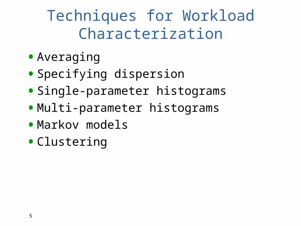
Techniques for Workload Characterization
•Averaging
•Specifying dispersion
•Single-parameter histograms
•Multi-parameter histograms
•Markov models
•Clustering
6
Averaging
•Characterize workload with average– Ex: Average number of network hops
•Arithmetic mean may be inappropriate– Ex: average hops may be a fraction– Ex: data may be skewed– Specify with median, mode
7
Case Study (1 of 2)
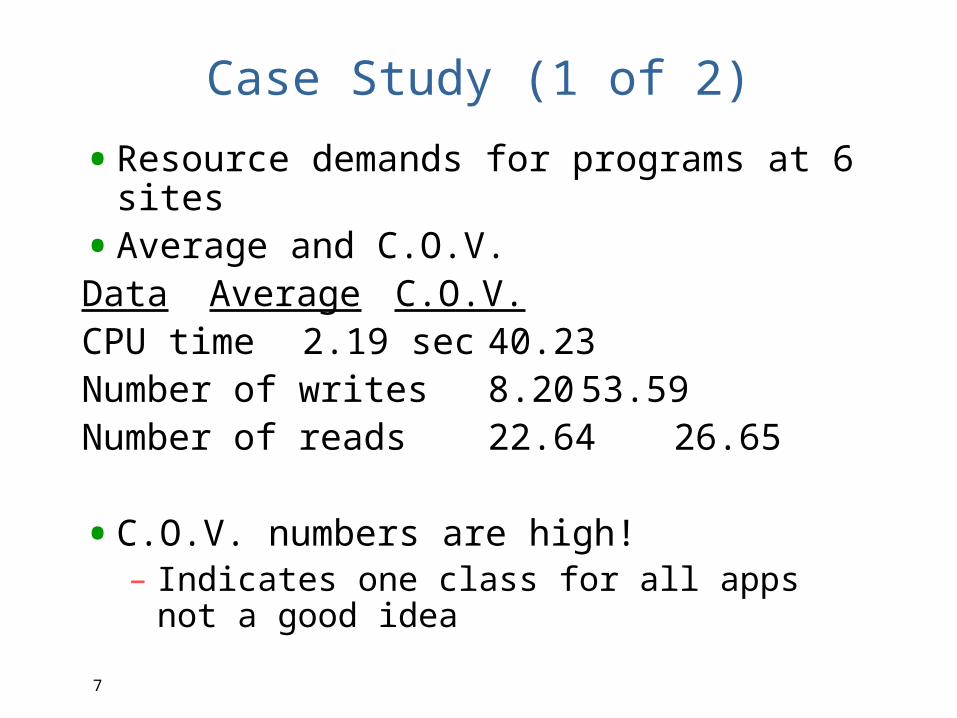
•Resource demands for programs at 6 sites
•Average and C.O.V.Data Average C.O.V.CPU time 2.19 sec 40.23Number of writes8.20 53.59Number of reads 22.64 26.65
•C.O.V. numbers are high!– Indicates one class for all apps not a good
idea
8
Case Study (2 of 2)
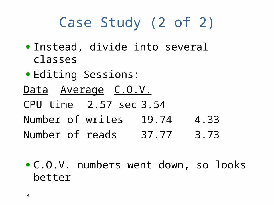
•Instead, divide into several classes
•Editing Sessions:Data Average C.O.V.CPU time 2.57 sec 3.54Number of writes19.74 4.33Number of reads 37.77 3.73
•C.O.V. numbers went down, so looks better
9
Techniques for Workload Characterization
•Averaging
•Specifying dispersion
•Single-parameter histograms
•Multi-parameter histograms
•Principal-component analysis
•Markov models
•Clustering
10
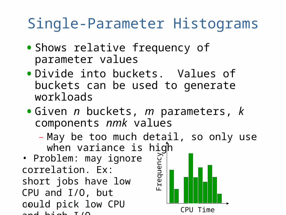
Single-Parameter Histograms
•Shows relative frequency of parameter values
•Divide into buckets. Values of buckets can be used to generate workloads
•Given n buckets, m parameters, k components nmk values– May be too much detail, so only use
when variance is high
Frequency
CPU Time
• Problem: may ignore correlation. Ex: short jobs have low CPU and I/O, but could pick low CPU and high I/O
11
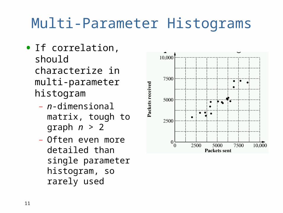
Multi-Parameter Histograms
• If correlation, should characterize in multi-parameter histogram– n-dimensional
matrix, tough to graph n > 2
– Often even more detailed than single parameter histogram, so rarely used
12
Techniques for Workload Characterization
•Averaging
•Specifying dispersion
•Single-parameter histograms
•Multi-parameter histograms
•Principal-component analysis
•Markov models
•Clustering

13
Markov Models (1 of 2)•Sometimes, important not to just have
number of each type of request but also order of requests
•If next request depends upon previous request, then can use Markov model– Actually, more general. If next state
depends upon current state
•Ex: process between CPU, disk, terminal:
(Draw diagramFig 6.4)
14
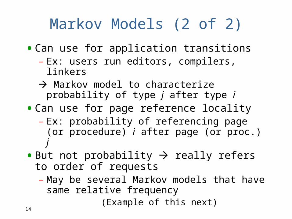
Markov Models (2 of 2)
•Can use for application transitions– Ex: users run editors, compilers, linkers Markov model to characterize
probability of type j after type i
•Can use for page reference locality– Ex: probability of referencing page (or
procedure) i after page (or proc.) j
•But not probability really refers to order of requests– May be several Markov models that have
same relative frequency(Example of this next)
15
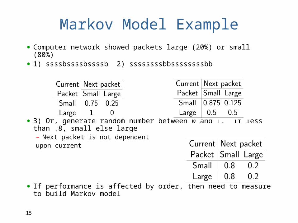
Markov Model Example
• Computer network showed packets large (20%) or small (80%)
• 1) ssssbssssbssssb 2) ssssssssbbssssssssbb
• 3) Or, generate random number between 0 and 1. If less than .8, small else large– Next packet is not dependentupon current
• If performance is affected by order, then need to measure to build Markov model
16
Techniques for Workload Characterization
•Averaging
•Specifying dispersion
•Single-parameter histograms
•Multi-parameter histograms
•Principal-component analysis
•Markov models
•Clustering
17
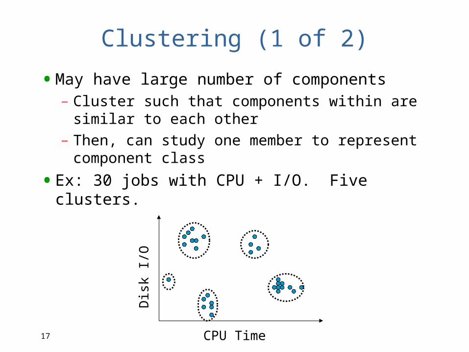
Clustering (1 of 2)
•May have large number of components– Cluster such that components within are
similar to each other– Then, can study one member to represent
component class
•Ex: 30 jobs with CPU + I/O. Five clusters.
Dis
k I/O
CPU Time
18
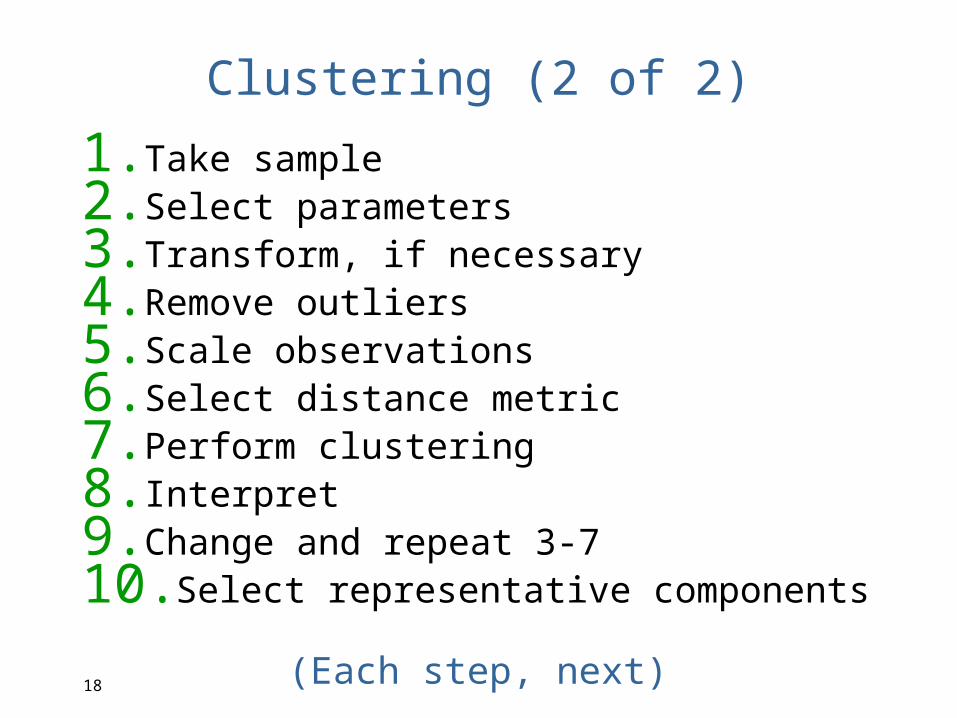
Clustering (2 of 2)
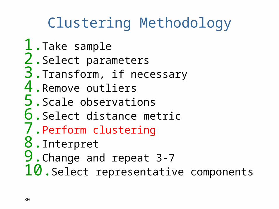
1.Take sample2.Select parameters3.Transform, if necessary4.Remove outliers5.Scale observations6.Select distance metric7.Perform clustering8.Interpret9.Change and repeat 3-710.Select representative components
(Each step, next)
19
Clustering: Sampling
•Usually too many components to do clustering analysis– That’s why we are doing clustering in the
first place!
•Select small subset– If careful, will show similar behavior to
the rest
•May choose randomly– However, if are interested in a specific
aspect, may choose to cluster only those•Ex: if interested in a disk, only do
clustering analysis on components with high I/O
20
Clustering: Parameter Selection
•Many components have a large number of parameters (resource demands)– Some important, some not– Remove the ones that do not matter
•Two key criteria: impact on perf & variance– If have no impact, omit. Ex: Lines of
output – If have little variance, omit. Ex: Processes
created
•Method: redo clustering with 1 less parameter. Count fraction that change cluster membership. If not many change, remove parameter.
21
Clustering: Transformation
•If distribution is skewed, may want to transform the measure of the parameter
•Ex: one study measured CPU time– Two programs taking 1 and 2 seconds
are as different as two programs taking 10 and 20 milliseconds
Take ratio of CPU time and not difference
(More in Chapter 15)
22
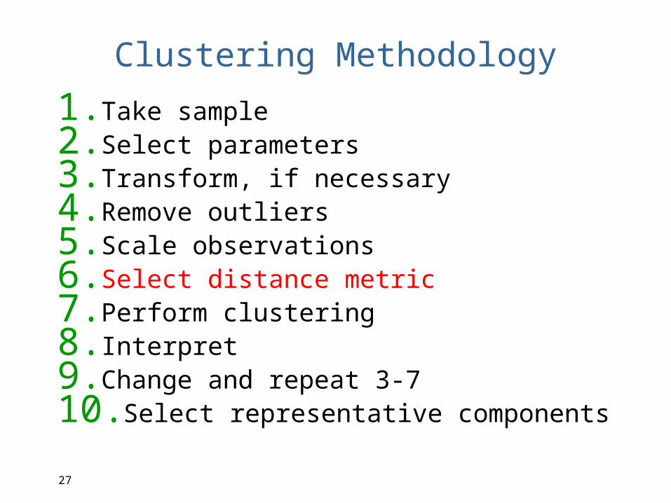
Clustering Methodology
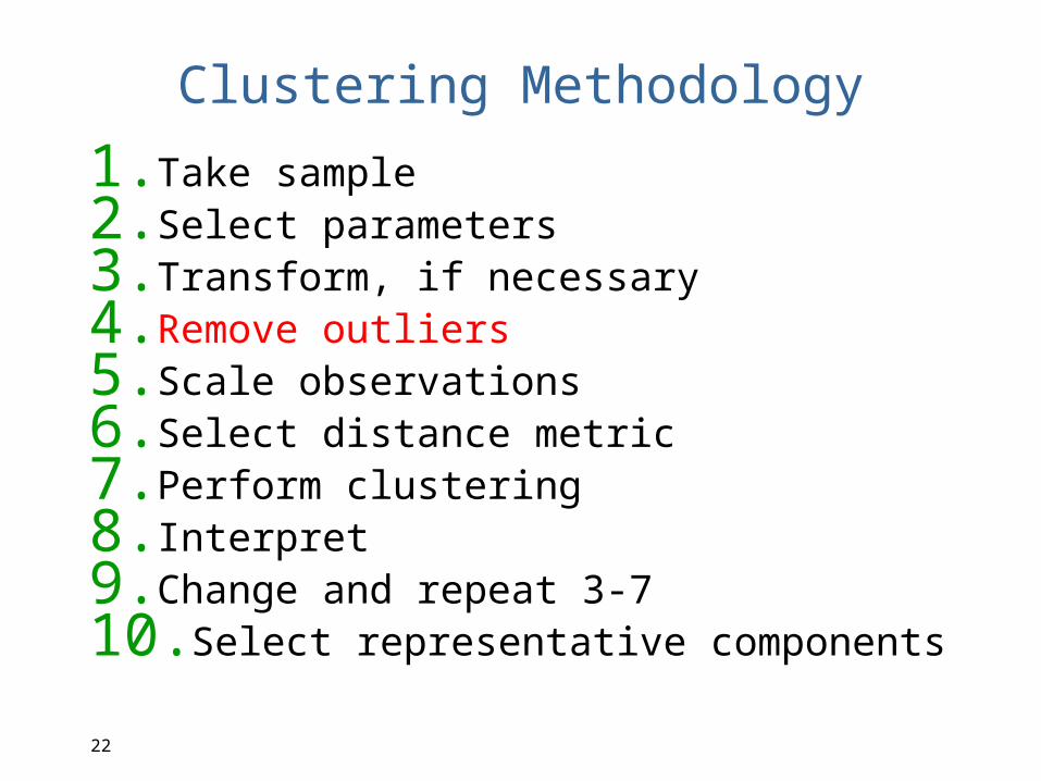
1.Take sample2.Select parameters3.Transform, if necessary4.Remove outliers5.Scale observations6.Select distance metric7.Perform clustering8.Interpret9.Change and repeat 3-710.Select representative components
23
Clustering: Outliers
•Data points with extreme parameter values
•Can significantly affect max or min (or mean or variance)
•For normalization (scaling, next) their inclusion/exclusion may significantly affect outcome
•Only exclude if do not consume significant portion of resources– Ex: extremely high RTT flows, exclude– Ex: extremely long (heavy tail) flow, include
24
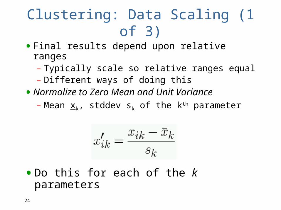
Clustering: Data Scaling (1 of 3)
•Final results depend upon relative ranges– Typically scale so relative ranges equal– Different ways of doing this
•Normalize to Zero Mean and Unit Variance– Mean xk, stddev sk of the kth parameter
•Do this for each of the k parameters
25
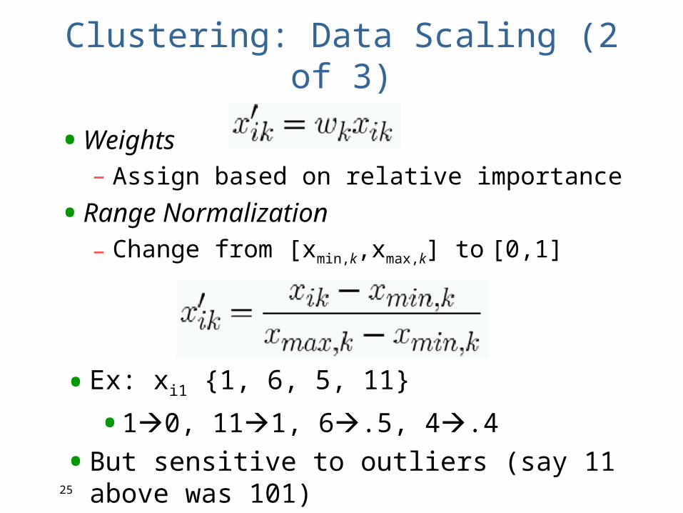
Clustering: Data Scaling (2 of 3)
•Weights– Assign based on relative importance
•Range Normalization– Change from [xmin,k,xmax,k] to [0,1]
•Ex: xi1 {1, 6, 5, 11}
•10, 111, 6.5, 4.4
•But sensitive to outliers (say 11 above was 101)
26
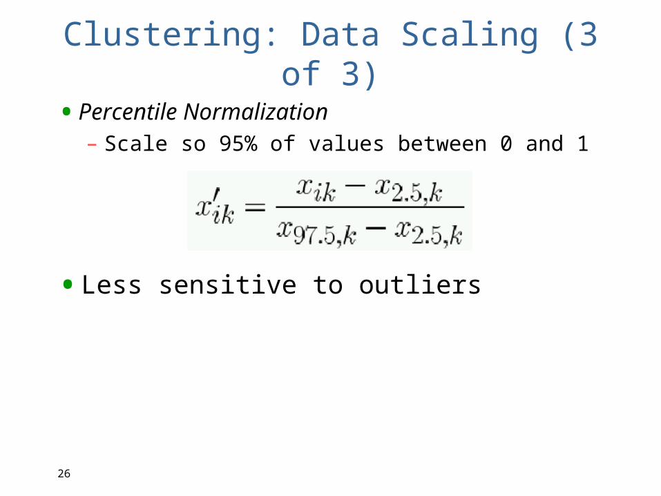
Clustering: Data Scaling (3 of 3)
•Percentile Normalization– Scale so 95% of values between 0 and 1
•Less sensitive to outliers
27
Clustering Methodology
1.Take sample2.Select parameters3.Transform, if necessary4.Remove outliers5.Scale observations6.Select distance metric7.Perform clustering8.Interpret9.Change and repeat 3-710.Select representative components
28
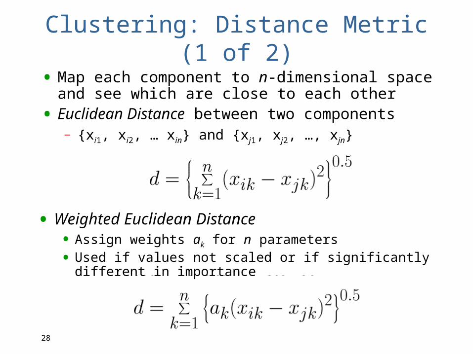
Clustering: Distance Metric (1 of 2)
• Map each component to n-dimensional space and see which are close to each other
• Euclidean Distance between two components– {xi1, xi2, … xin} and {xj1, xj2, …, xjn}
• Weighted Euclidean Distance• Assign weights ak for n parameters
• Used if values not scaled or if significantly different in importance
29
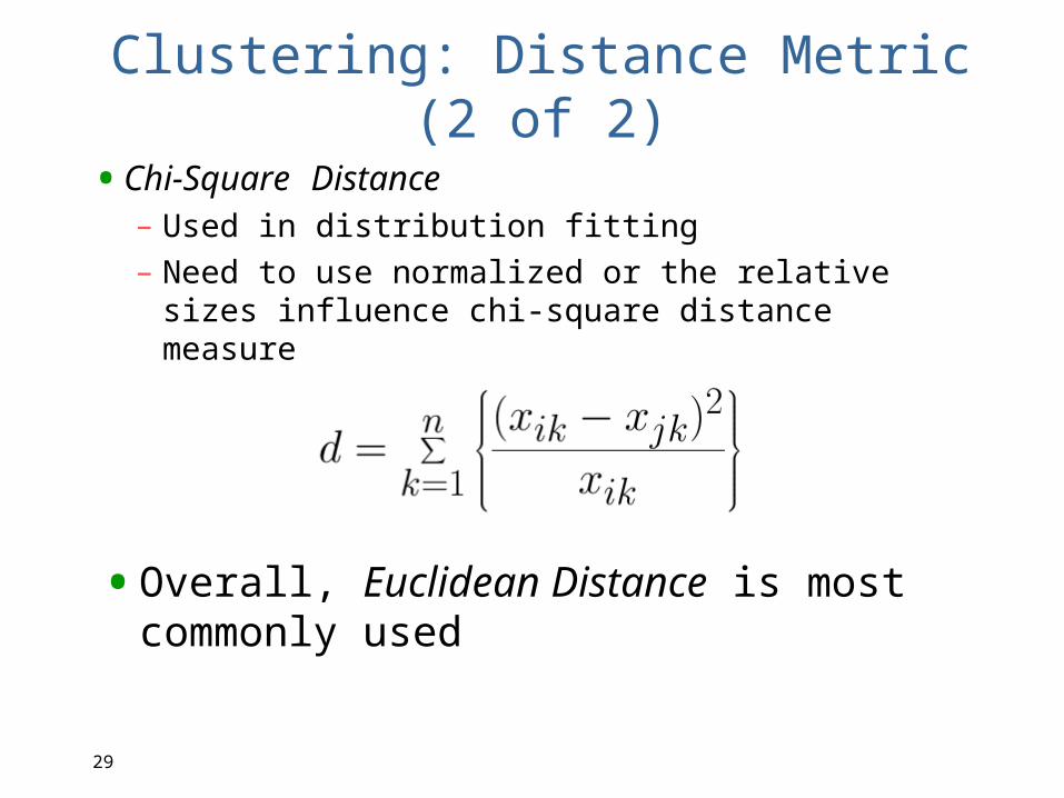
Clustering: Distance Metric (2 of 2)
•Chi-Square Distance– Used in distribution fitting – Need to use normalized or the relative sizes
influence chi-square distance measure
•Overall, Euclidean Distance is most commonly used
30
Clustering Methodology
1.Take sample2.Select parameters3.Transform, if necessary4.Remove outliers5.Scale observations6.Select distance metric7.Perform clustering8.Interpret9.Change and repeat 3-710.Select representative components
31
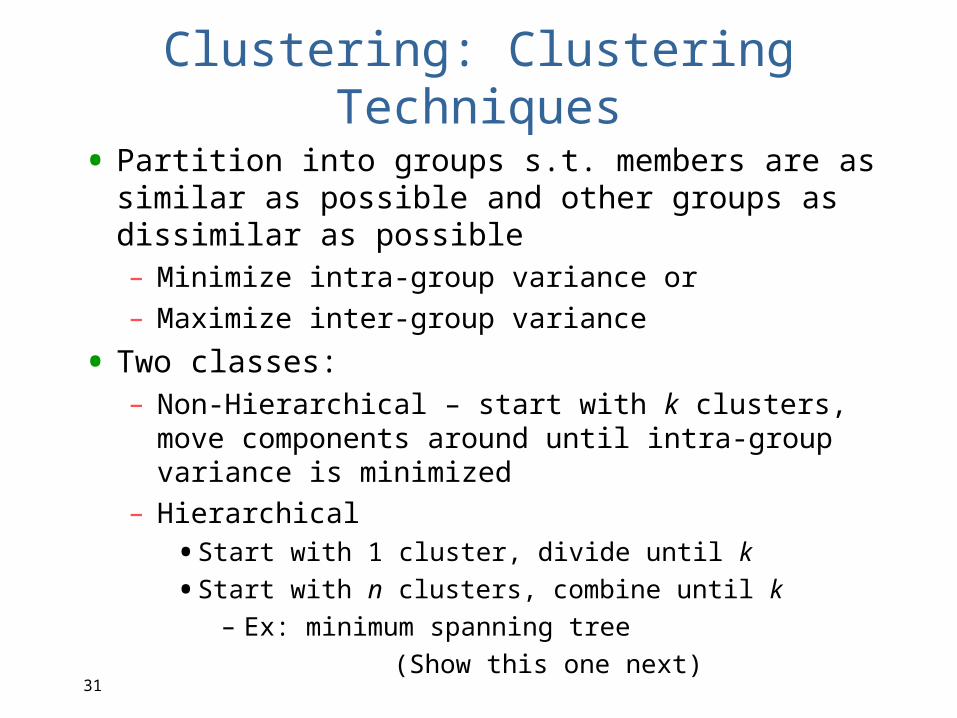
Clustering: Clustering Techniques
• Partition into groups s.t. members are as similar as possible and other groups as dissimilar as possible– Minimize intra-group variance or– Maximize inter-group variance
• Two classes:– Non-Hierarchical – start with k clusters, move
components around until intra-group variance is minimized
– Hierarchical•Start with 1 cluster, divide until k
•Start with n clusters, combine until k– Ex: minimum spanning tree
(Show this one next)
32
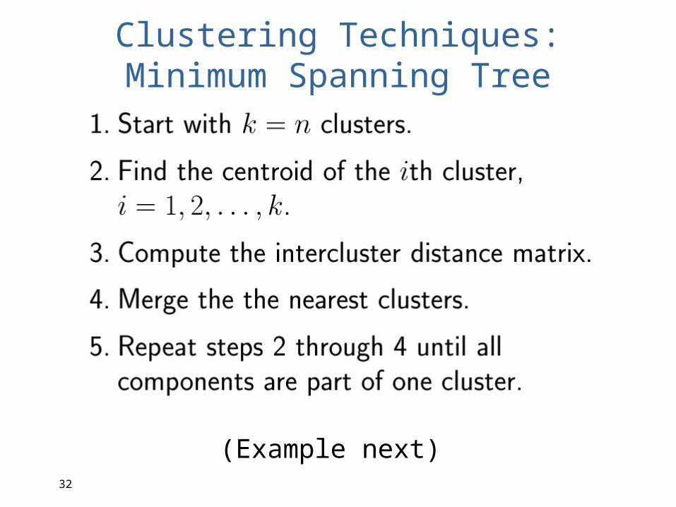
Clustering Techniques: Minimum Spanning Tree
(Example next)
33
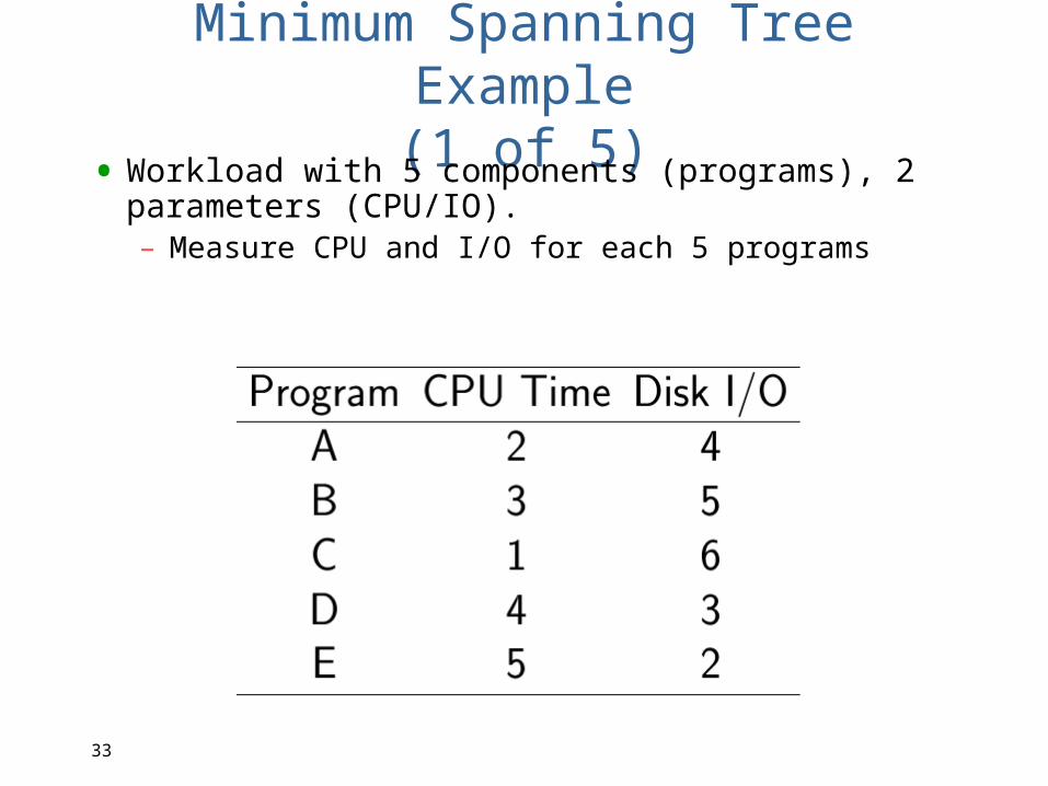
Minimum Spanning Tree Example(1 of 5)• Workload with 5 components (programs), 2
parameters (CPU/IO).– Measure CPU and I/O for each 5 programs
34
Minimum Spanning Tree Example(2 of 5)
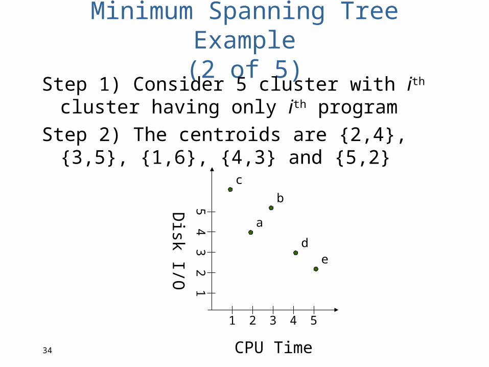
Step 1) Consider 5 cluster with ith cluster having only ith program
Step 2) The centroids are {2,4}, {3,5}, {1,6}, {4,3} and {5,2}
1 2 43 5
12
43
5
Disk I/O
CPU Time
c
a
b
de
35
Minimum Spanning Tree Example(3 of 5)
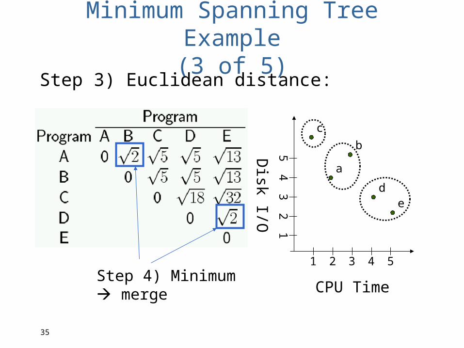
Step 3) Euclidean distance:
1 2 43 5
12
43
5
Disk I/O
CPU Time
c
a
b
de
Step 4) Minimum merge
36
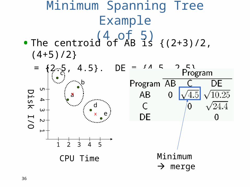
Minimum Spanning Tree Example(4 of 5)•The centroid of AB is {(2+3)/2, (4+5)/2}
= {2.5, 4.5}. DE = {4.5, 2.5}
1 2 43 5
12
43
5
Disk I/O
CPU Time
c
a
b
dex
x
Minimum merge
37
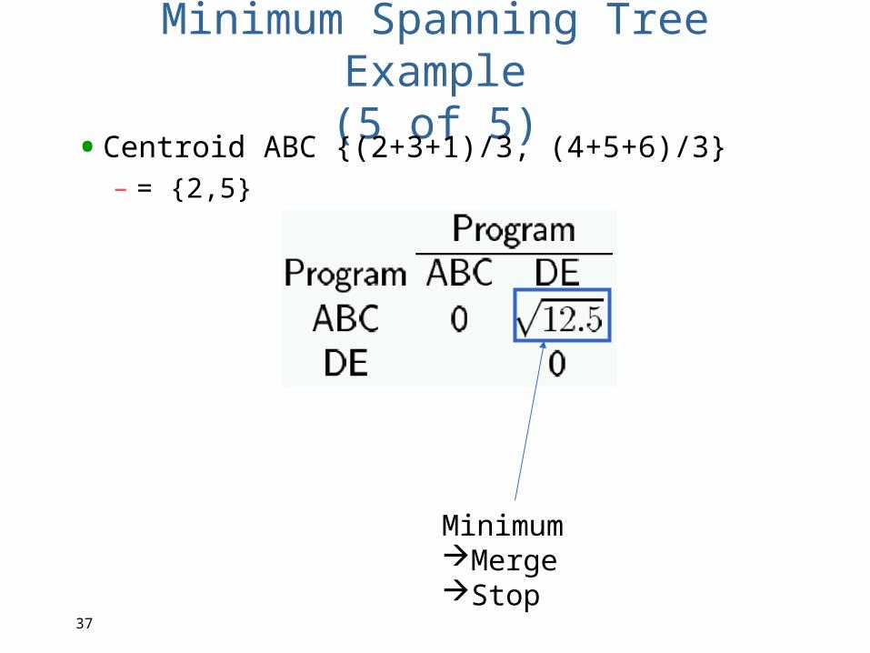
Minimum Spanning Tree Example(5 of 5)•Centroid ABC {(2+3+1)/3, (4+5+6)/3}
– = {2,5}
MinimumMergeStop
38
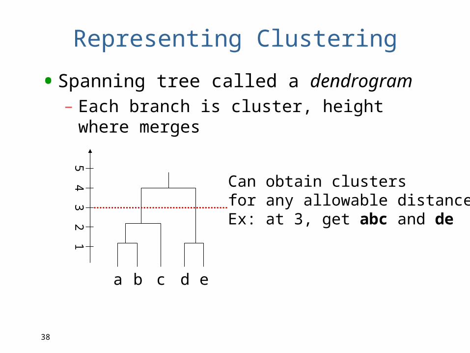
Representing Clustering
•Spanning tree called a dendrogram– Each branch is cluster, height where
merges
12
43
5
a b c d e
Can obtain clustersfor any allowable distanceEx: at 3, get abc and de
39
Interpreting Clusters
•Clusters will small populations may be discarded– If use few resources– If cluster with 1 component uses 50% of
resources, cannot discard!
•Name clusters, often by resource demands– Ex: “CPU bound” or “I/O bound”
•Select 1+ components from each cluster as a test workload– Can make number selected proportional
to cluster size, total resource demands or other