adapted from menascé & almeida.1 workload characterization for the web
TRANSCRIPT
Adapted from Menascé & Almeida. 1
Workload Characterization for
the Web
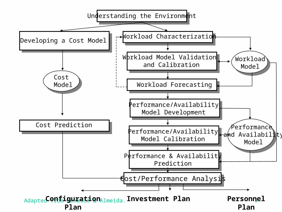
Adapted from Menascé & Almeida. 2Configuration Plan Investment Plan Personnel Plan
Understanding the Environment
Workload Characterization
WorkloadModel
Workload Model Validation and Calibration
Workload Forecasting
Cost Prediction
Cost Model
Developing a Cost Model
Performance and Availability
Model
Cost/Performance Analysis
Performance/AvailabilityModel Development
Performance/AvailabilityModel Calibration
Performance & AvailabilityPrediction
Adapted from Menascé & Almeida. 3
Learning Objectives (1)
� Introduce the workload characterization problem.
� Discuss a simple example of characterizing the workload for an intranet.
� Present a workload characterization methodology.
Adapted from Menascé & Almeida. 4
Learning Objectives (2)
� Discuss the following steps:– analysis standpoint
– identification of the basic component
– choice of the characterizing parameters
– data collection
– partitioning the workload
� Characteristics of Web workloads: – burstiness
– heavy-tailed distributions
Adapted from Menascé & Almeida. 5
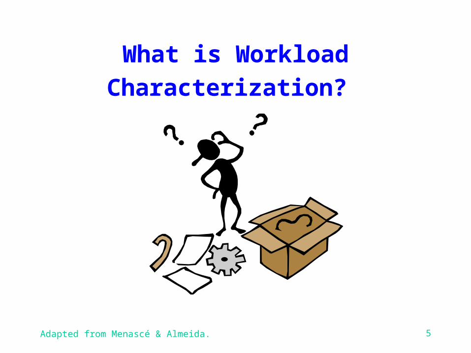
What is Workload
Characterization?
Adapted from Menascé & Almeida. 6
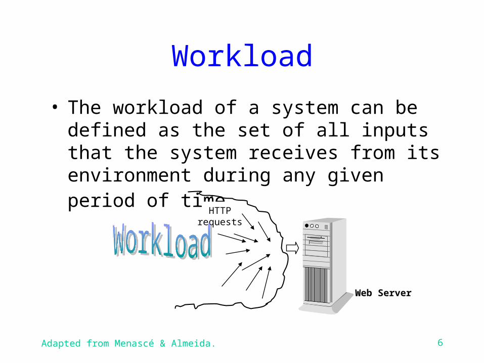
Workload
• The workload of a system can be defined as the set of all inputs that the system receives from its environment during any given period of time.
HTTPrequests
Web Server
Adapted from Menascé & Almeida. 7
Workload Characterization
• Depends on the purpose of the study– cost x benefit of a proxy caching server– impact of a faster CPU on the response time
• Common steps– specification of a point of view from the workload
will be analyzed;– choice of set of relevant parameters;– monitoring the system;– analysis and reduction of performance data– construction of a workload model.
Adapted from Menascé & Almeida. 8
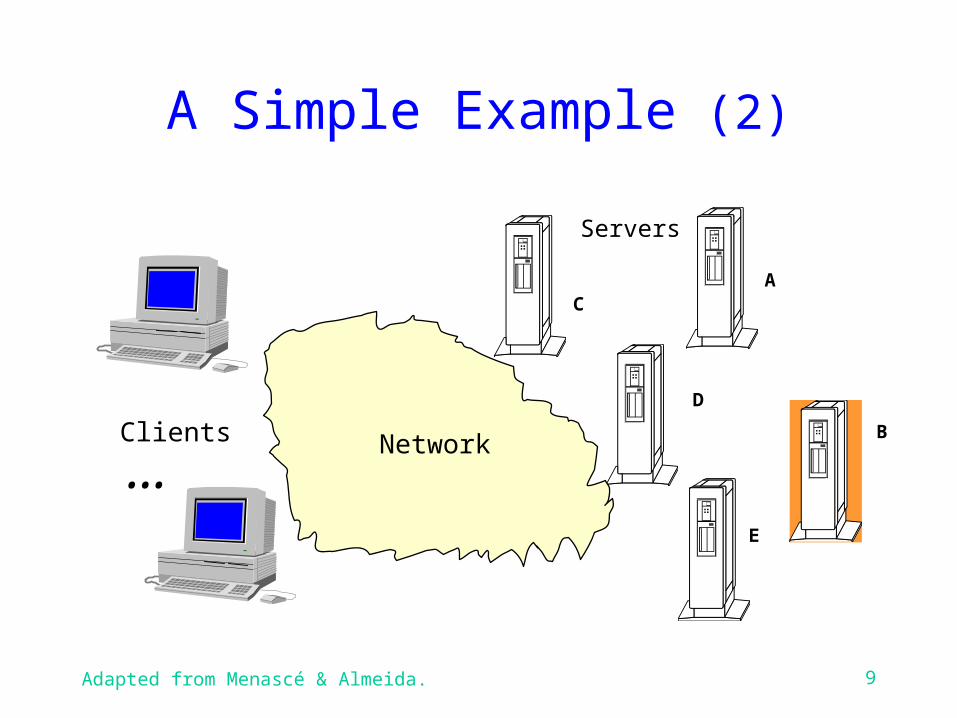
A Simple Example• A construction and engineering company is planning
to roll out new applications and to increase the number of employees that have access to the corporate intranet. The main applications are health human resources, insurance payments, on-demand interactive training, etc.
• Main problem: response time of the human resource system
Adapted from Menascé & Almeida. 9
A Simple Example (2)
A
D
E
C
BClients
Servers
Network...
Adapted from Menascé & Almeida. 10
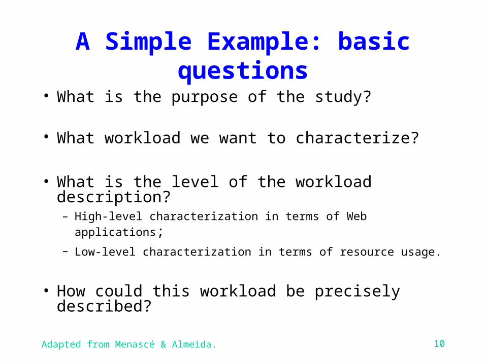
A Simple Example: basic questions
• What is the purpose of the study?
• What workload we want to characterize?
• What is the level of the workload description?– High-level characterization in terms of Web applications;– Low-level characterization in terms of resource usage.
• How could this workload be precisely described?
Adapted from Menascé & Almeida. 11
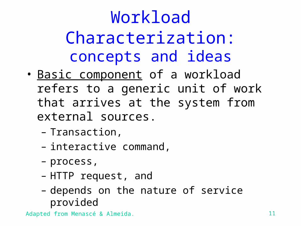
Workload Characterization: concepts and ideas
• Basic component of a workload refers to a generic unit of work that arrives at the system from external sources.– Transaction,– interactive command,– process,– HTTP request, and – depends on the nature of service provided
Adapted from Menascé & Almeida. 12
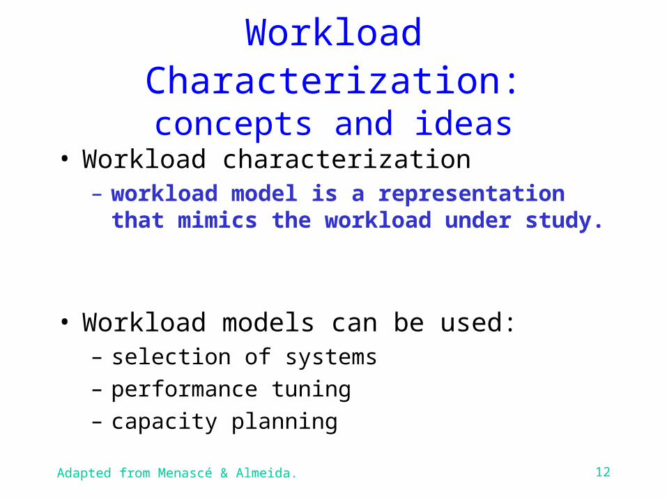
Workload Characterization: concepts and ideas
• Workload characterization – workload model is a representation that
mimics the workload under study.
• Workload models can be used:– selection of systems– performance tuning– capacity planning
Adapted from Menascé & Almeida. 13
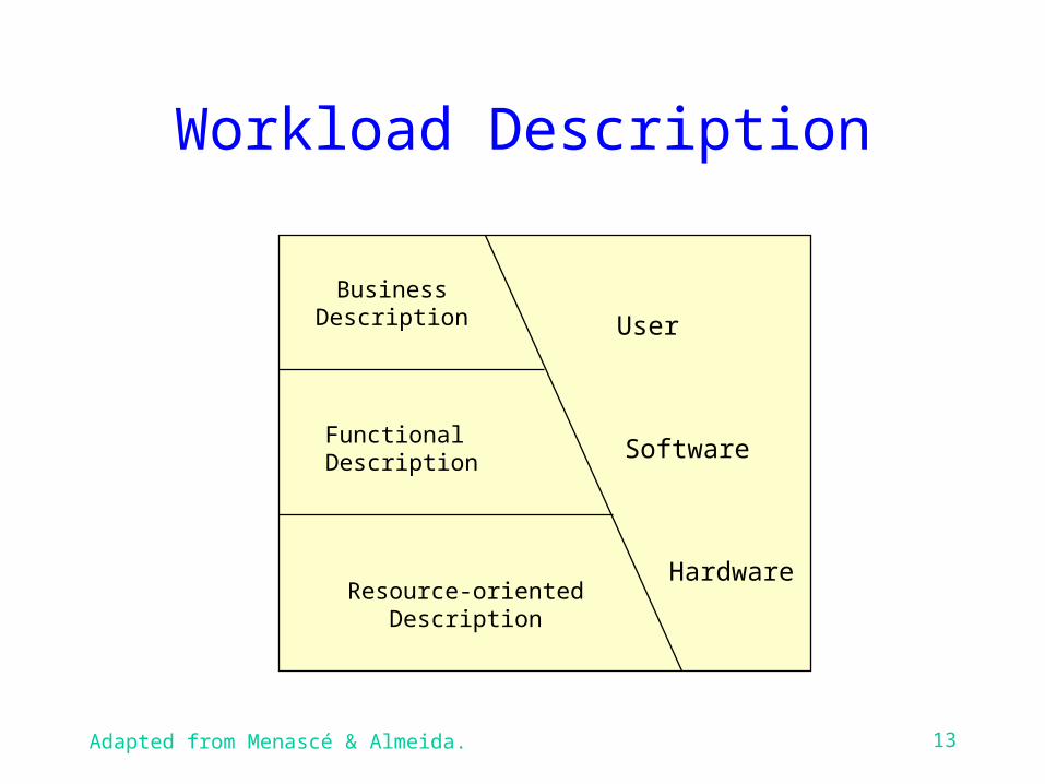
Workload Description
Hardware
Software
User
Resource-orientedDescription
Functional Description
BusinessDescription
Adapted from Menascé & Almeida. 14
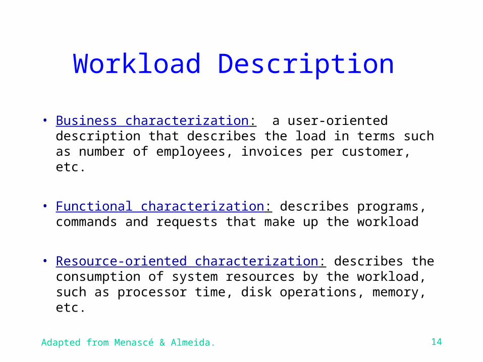
Workload Description
• Business characterization: a user-oriented description that describes the load in terms such as number of employees, invoices per customer, etc.
• Functional characterization: describes programs, commands and requests that make up the workload
• Resource-oriented characterization: describes the consumption of system resources by the workload, such as processor time, disk operations, memory, etc.
Adapted from Menascé & Almeida. 15
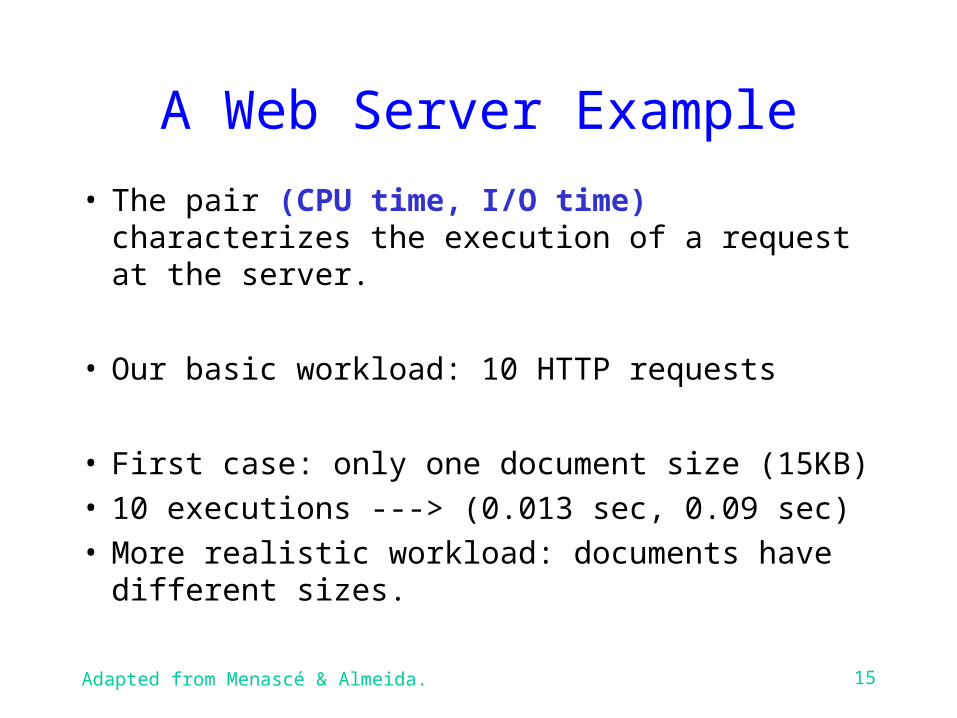
A Web Server Example
• The pair (CPU time, I/O time) characterizes the execution of a request at the server.
• Our basic workload: 10 HTTP requests
• First case: only one document size (15KB)• 10 executions ---> (0.013 sec, 0.09 sec)• More realistic workload: documents have
different sizes.
Adapted from Menascé & Almeida. 16
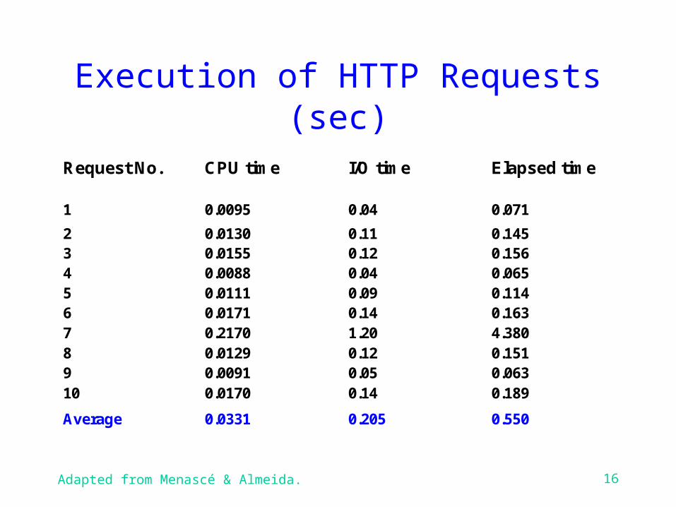
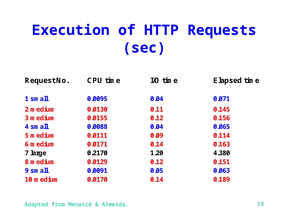
Execution of HTTP Requests (sec)
Request No. CPU time I/O time Elapsed time
1 0.0095 0.04 0.071
2 0.0130 0.11 0.1453 0.0155 0.12 0.1564 0.0088 0.04 0.0655 0.0111 0.09 0.1146 0.0171 0.14 0.1637 0.2170 1.20 4.3808 0.0129 0.12 0.1519 0.0091 0.05 0.06310 0.0170 0.14 0.189
Average 0.0331 0.205 0.550
Adapted from Menascé & Almeida. 17
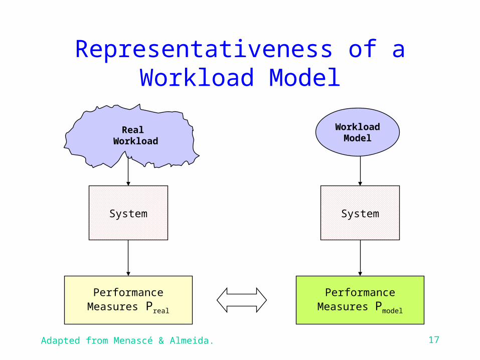
Representativeness of aWorkload Model
System
PerformanceMeasures Preal
System
PerformanceMeasures Pmodel
WorkloadModel
Real Workload
Adapted from Menascé & Almeida. 18
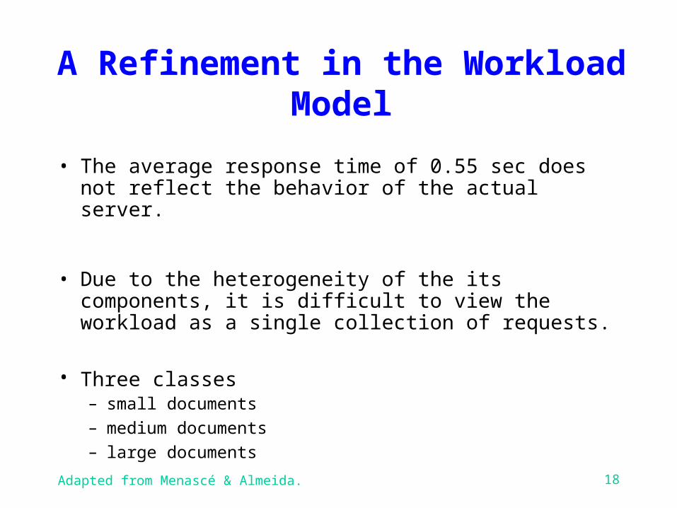
A Refinement in the Workload Model
• The average response time of 0.55 sec does not reflect the behavior of the actual server.
• Due to the heterogeneity of the its components, it is difficult to view the workload as a single collection of requests.
• Three classes– small documents – medium documents– large documents
Adapted from Menascé & Almeida. 19
Execution of HTTP Requests (sec)
Request No. CPU time I/O time Elapsed time
1 small 0.0095 0.04 0.071
2 medium 0.0130 0.11 0.1453 medium 0.0155 0.12 0.1564 small 0.0088 0.04 0.0655 medium 0.0111 0.09 0.1146 medium 0.0171 0.14 0.1637 large 0.2170 1.20 4.3808 medium 0.0129 0.12 0.1519 small 0.0091 0.05 0.06310 medium 0.0170 0.14 0.189
Adapted from Menascé & Almeida. 20
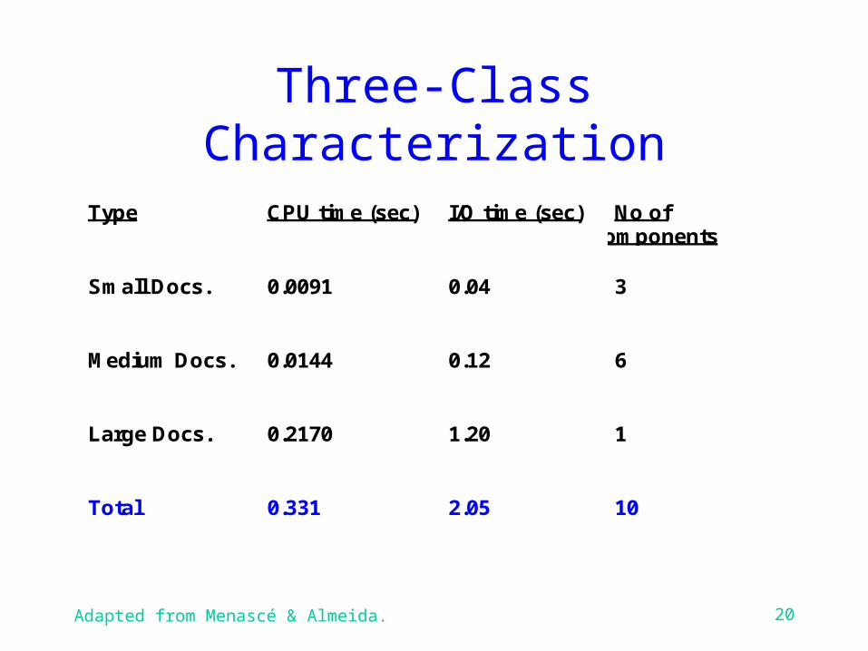
Three-Class Characterization
Type CPU time (sec) I/O time (sec) No ofomponents
Small Docs. 0.0091 0.04 3
Medium Docs. 0.0144 0.12 6
Large Docs. 0.2170 1.20 1
Total 0.331 2.05 10
Adapted from Menascé & Almeida. 21
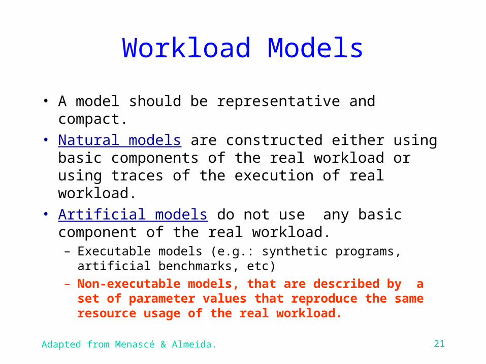
Workload Models
• A model should be representative and compact.• Natural models are constructed either using basic
components of the real workload or using traces of the execution of real workload.
• Artificial models do not use any basic component of the real workload.– Executable models (e.g.: synthetic programs, artificial
benchmarks, etc)– Non-executable models, that are described by a set of
parameter values that reproduce the same resource usage of the real workload.
Adapted from Menascé & Almeida. 22
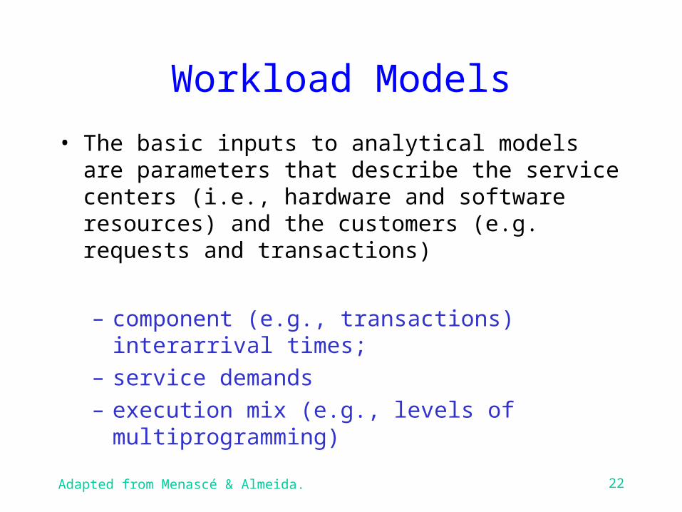
Workload Models
• The basic inputs to analytical models are parameters that describe the service centers (i.e., hardware and software resources) and the customers (e.g. requests and transactions)
– component (e.g., transactions) interarrival times;– service demands– execution mix (e.g., levels of multiprogramming)
Adapted from Menascé & Almeida. 23
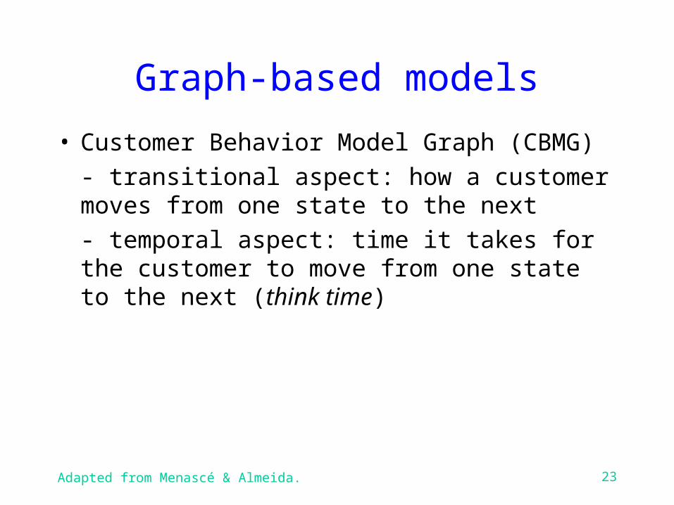
Graph-based models
• Customer Behavior Model Graph (CBMG)
- transitional aspect: how a customer moves from one state to the next
- temporal aspect: time it takes for the customer to move from one state to the next (think time)
Adapted from Menascé & Almeida. 24
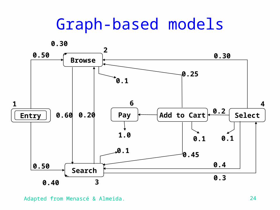
Graph-based models
Entry
Browse
Search
Pay Add to Cart Select
1
0.50
0.50
3
0.1
0.1
1.0
6
0.20 0.2
0.1 0.1
0.45
0.4
0.3
20.30
0.25
4
0.60
0.30
0.40
Adapted from Menascé & Almeida. 25
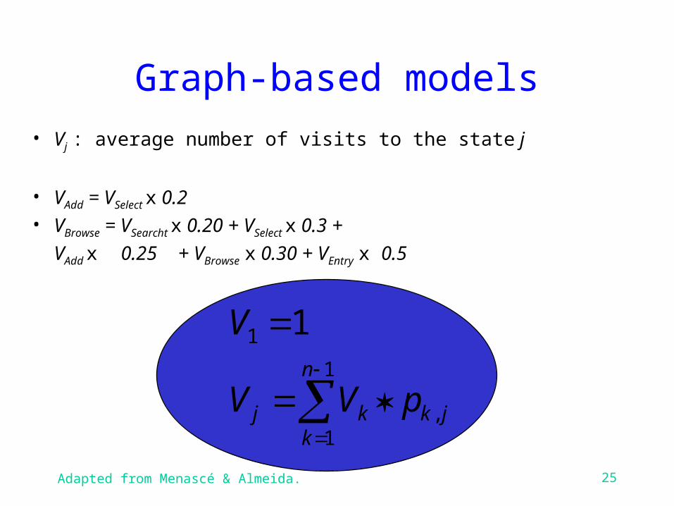
Graph-based models
• Vj : average number of visits to the state j
• VAdd = VSelect x 0.2• VBrowse = VSearcht x 0.20 + VSelect x 0.3 +
VAdd x 0.25 + VBrowse x 0.30 + VEntry x 0.5
jk
n
kkj pVV
V
,
1
1
1 1
Adapted from Menascé & Almeida. 26
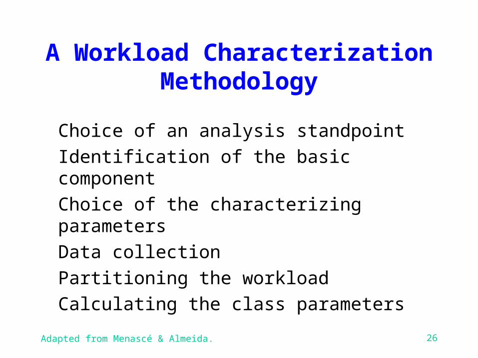
A Workload Characterization Methodology
� Choice of an analysis standpoint� Identification of the basic component� Choice of the characterizing parameters� Data collection� Partitioning the workload� Calculating the class parameters
Adapted from Menascé & Almeida. 27
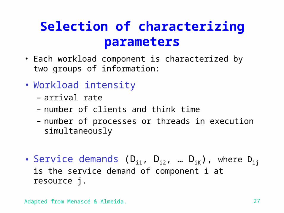
Selection of characterizing parameters
• Each workload component is characterized by two groups of information:
• Workload intensity– arrival rate– number of clients and think time– number of processes or threads in execution
simultaneously
• Service demands (Di1, Di2, … DiK), where Dij is
the service demand of component i at resource j.
Adapted from Menascé & Almeida. 28
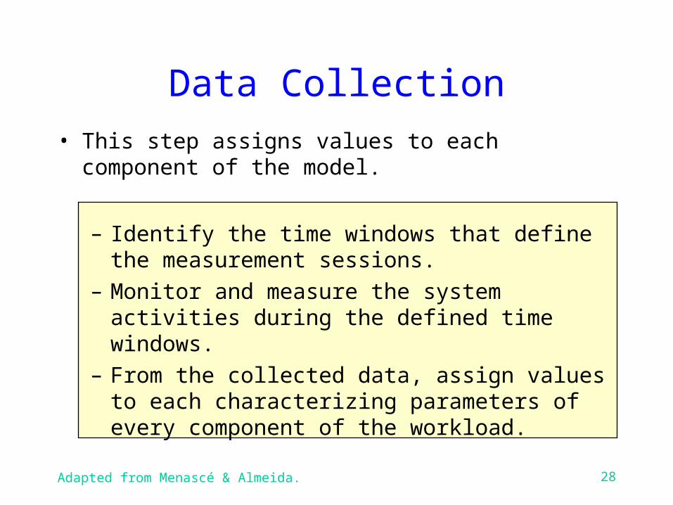
Data Collection• This step assigns values to each component of the
model.
– Identify the time windows that define the measurement sessions.
– Monitor and measure the system activities during the defined time windows.
– From the collected data, assign values to each characterizing parameters of every component of the workload.
Adapted from Menascé & Almeida. 29
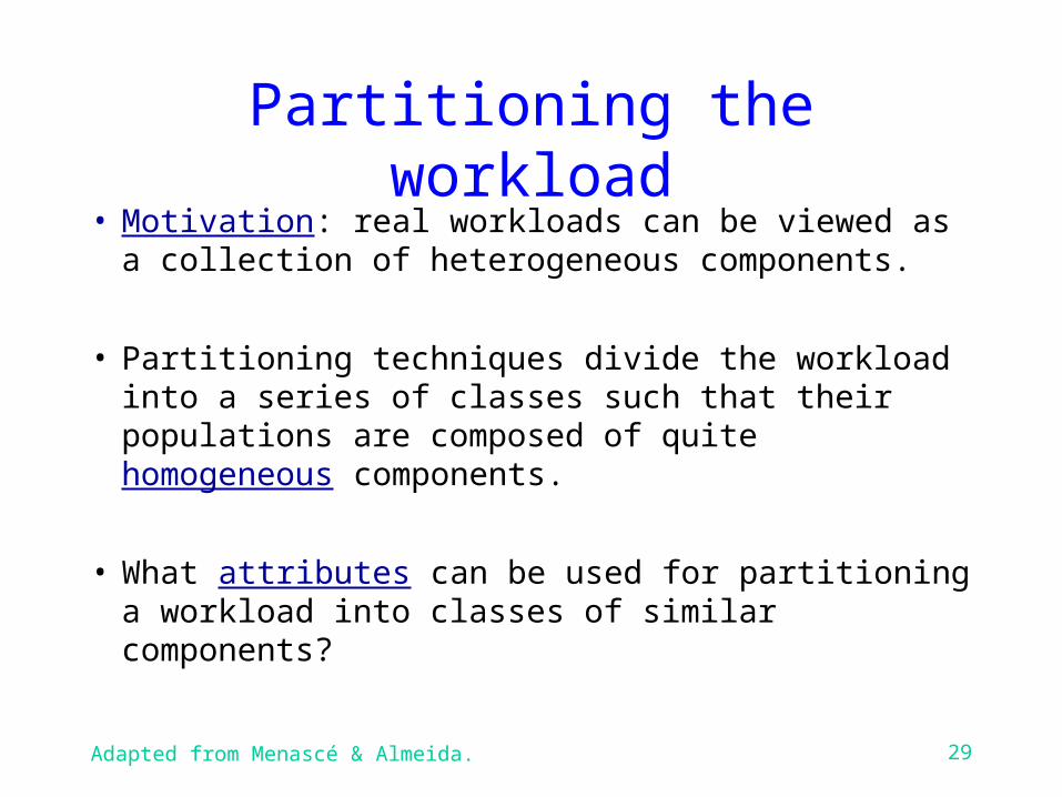
Partitioning the workload• Motivation: real workloads can be viewed as a
collection of heterogeneous components.
• Partitioning techniques divide the workload into a series of classes such that their populations are composed of quite homogeneous components.
• What attributes can be used for partitioning a workload into classes of similar components?
Adapted from Menascé & Almeida. 30
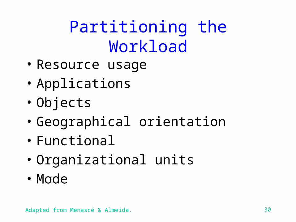
Partitioning the Workload
• Resource usage
• Applications
• Objects
• Geographical orientation
• Functional
• Organizational units
• Mode
Adapted from Menascé & Almeida. 31
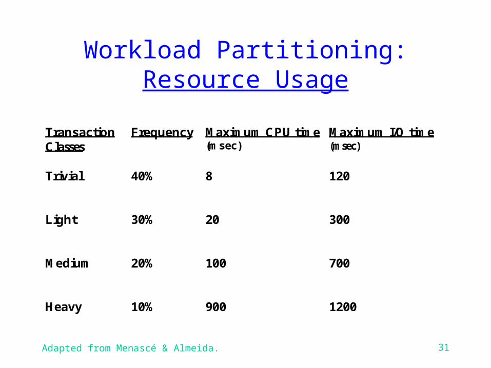
Workload Partitioning:Resource Usage
TransactionClasses
Frequency Maximum CPU time(msec)
Maximum I/O time(msec)
Trivial 40% 8 120
Light 30% 20 300
Medium 20% 100 700
Heavy 10% 900 1200
Adapted from Menascé & Almeida. 32
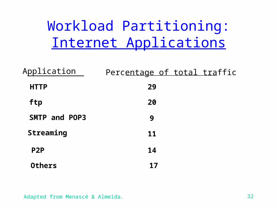
Workload Partitioning:Internet Applications
Application Percentage of total traffic
HTTP 29
ftp 20
SMTP and POP3 9
Streaming 11
Others 17
P2P 14
Adapted from Menascé & Almeida. 33
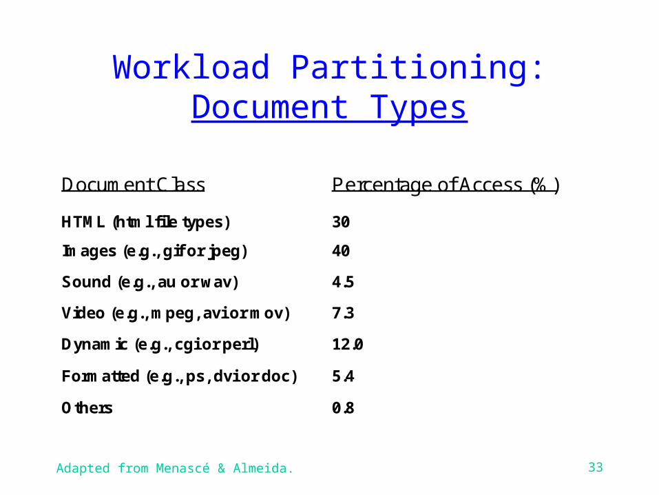
Workload Partitioning:Document Types
Document Class Percentage of Access (%)
HTML (html file types) 30
Images (e.g., gif or jpeg) 40
Sound (e.g., au or wav) 4.5
Video (e.g., mpeg, avi or mov) 7.3
Dynamic (e.g., cgi or perl) 12.0
Formatted (e.g., ps, dvi or doc) 5.4
Others 0.8
Adapted from Menascé & Almeida. 34
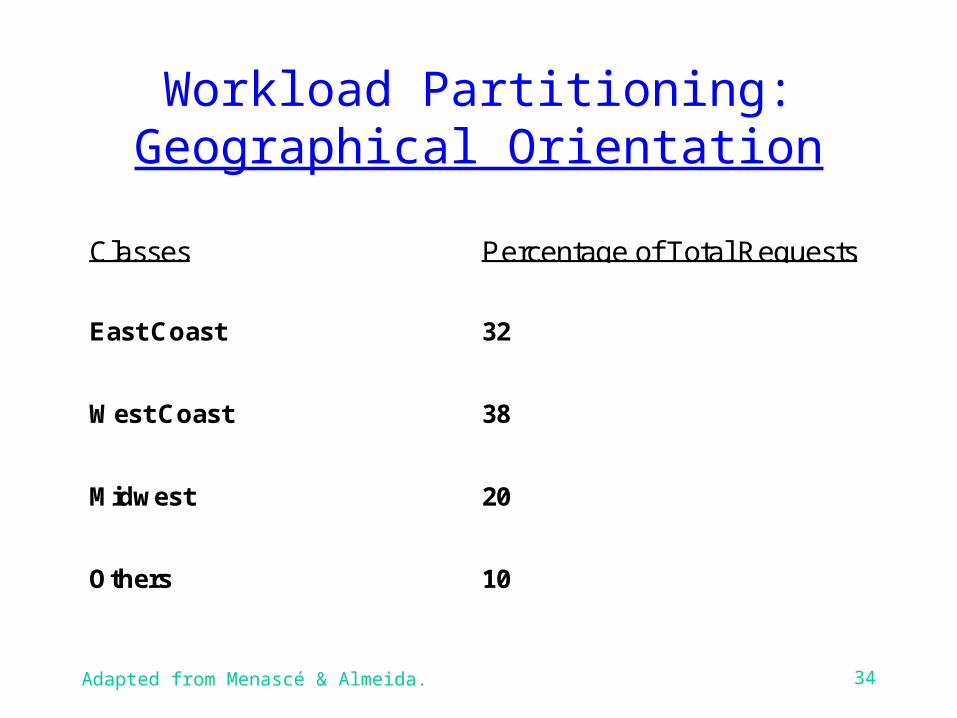
Workload Partitioning:Geographical Orientation
Classes Percentage of Total Requests
East Coast 32
West Coast 38
Midwest 20
Others 10
Adapted from Menascé & Almeida. 35
Calculating the class parameters
• How should one calculate the parameter values that represent a class of components?
– Averaging: when a class consists of homogeneous components concerning service demands, an average of the parameter values of all components may be used.
– Clustering of workloads is a process in which a large number of components are grouped into clusters of similar components.
Adapted from Menascé & Almeida. 36
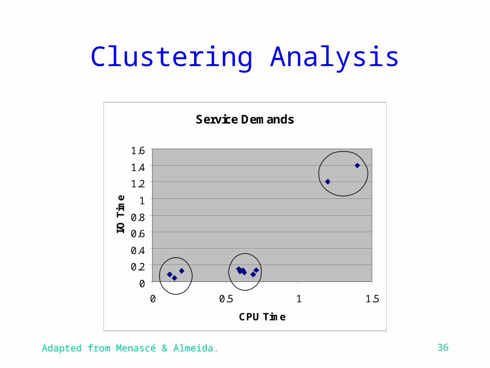
Clustering Analysis
Service Demands
0
0.2
0.4
0.6
0.8
1
1.2
1.4
1.6
0 0.5 1 1.5
CPU Time
I/O T
ime
Adapted from Menascé & Almeida. 37
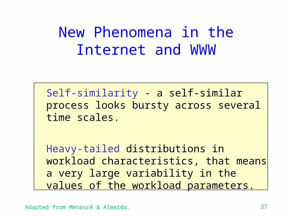
New Phenomena in the Internet and WWW
� Self-similarity - a self-similar process looks bursty across several time scales.
� Heavy-tailed distributions in workload characteristics, that means a very large variability in the values of the workload parameters.
Adapted from Menascé & Almeida. 38
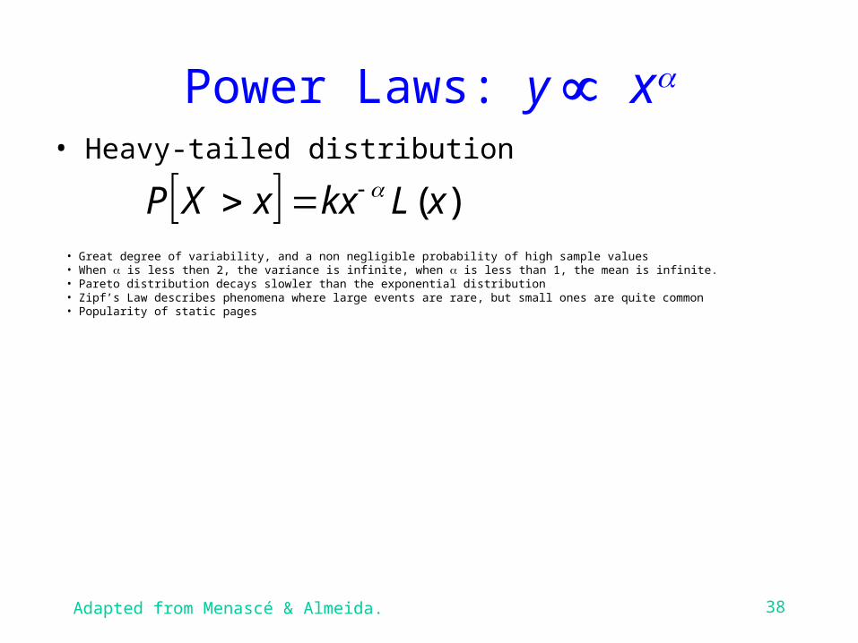
Power Laws: y x
• Heavy-tailed distribution )(xLkxxXP
• Great degree of variability, and a non negligible probability of high sample values• When is less then 2, the variance is infinite, when is less than 1, the mean is infinite.• Pareto distribution decays slowler than the exponential distribution• Zipf’s Law describes phenomena where large events are rare, but small ones are quite common• Popularity of static pages

Adapted from Menascé & Almeida. 39
WWW Traffic Burst
106
107
Bytes
Chronological time (slots of 1000 sec)
Adapted from Menascé & Almeida. 40
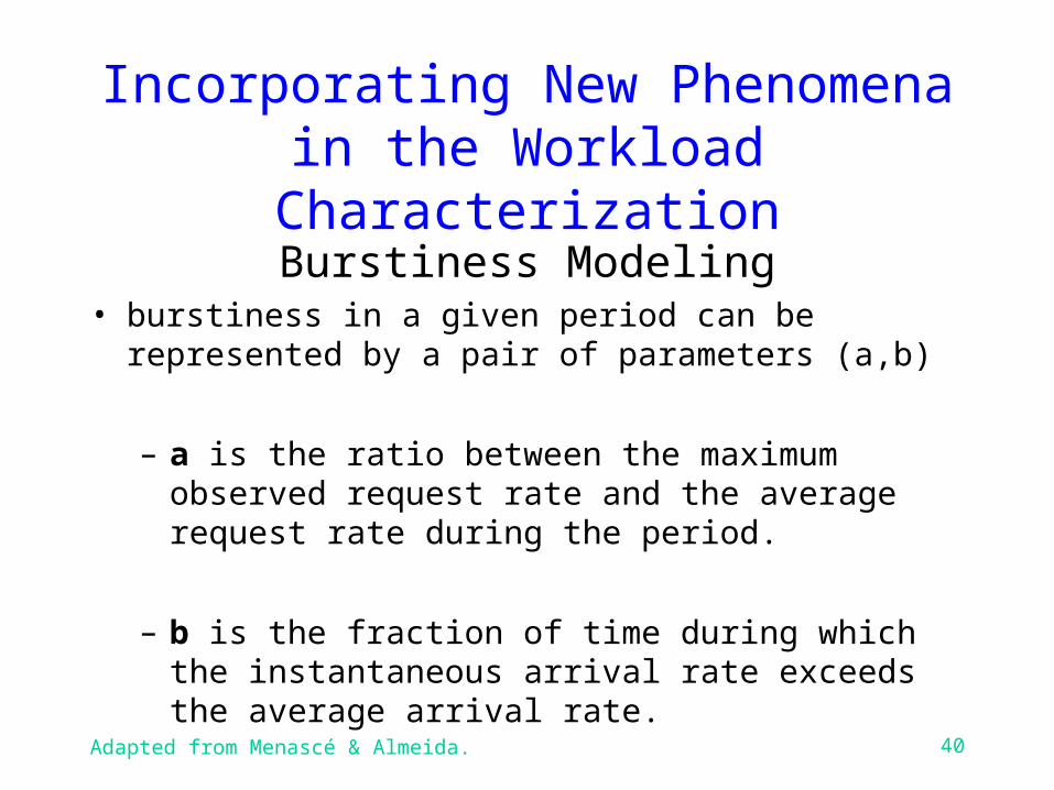
Incorporating New Phenomena in the Workload Characterization
Burstiness Modeling• burstiness in a given period can be represented by a
pair of parameters (a,b)
– a is the ratio between the maximum observed request rate and the average request rate during the period.
– b is the fraction of time during which the instantaneous arrival rate exceeds the average arrival rate.
Adapted from Menascé & Almeida. 41
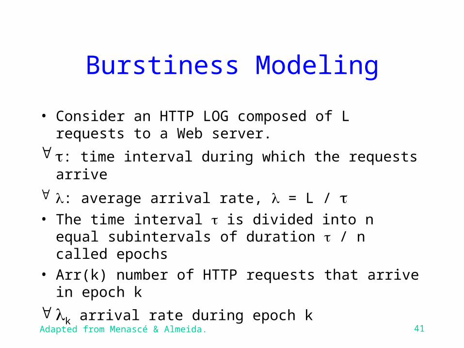
Burstiness Modeling
• Consider an HTTP LOG composed of L requests to a Web server.
: time interval during which the requests arrive
: average arrival rate, = L / • The time interval is divided into n equal subintervals
of duration / n called epochs• Arr(k) number of HTTP requests that arrive in epoch
k
k arrival rate during epoch k
Adapted from Menascé & Almeida. 42
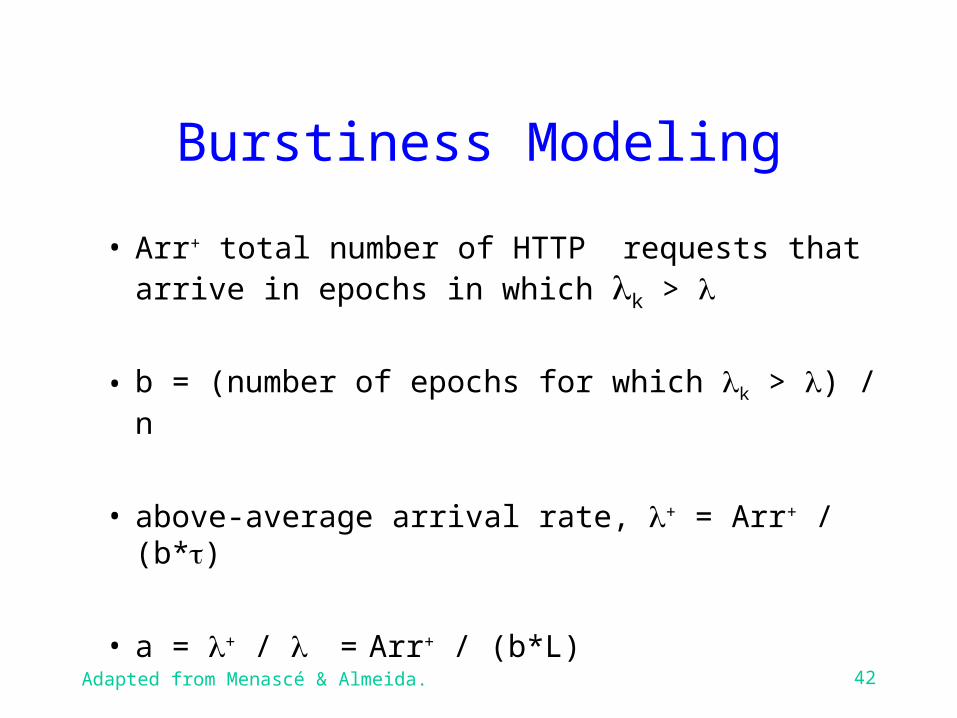
Burstiness Modeling
• Arr+ total number of HTTP requests that arrive in epochs in which k >
• b = (number of epochs for which k > ) / n
• above-average arrival rate, + = Arr+ / (b*)
• a = + / = Arr+ / (b*L)
Adapted from Menascé & Almeida. 43
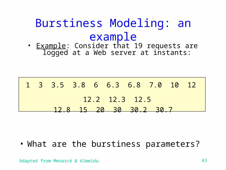
Burstiness Modeling: an example• Example: Consider that 19 requests are logged at a
Web server at instants:
1 3 3.5 3.8 6 6.3 6.8 7.0 10 12 12.2 12.3 12.5
12.8 15 20 30 30.2 30.7
• What are the burstiness parameters?
Adapted from Menascé & Almeida. 44
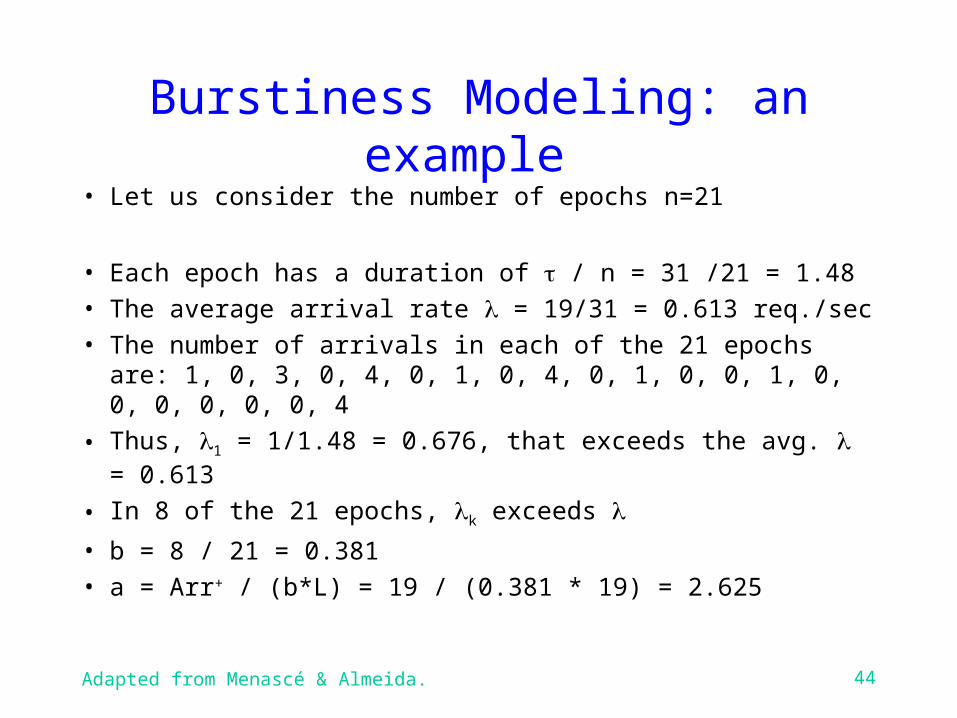
Burstiness Modeling: an example • Let us consider the number of epochs n=21
• Each epoch has a duration of / n = 31 /21 = 1.48• The average arrival rate = 19/31 = 0.613 req./sec• The number of arrivals in each of the 21 epochs are: 1,
0, 3, 0, 4, 0, 1, 0, 4, 0, 1, 0, 0, 1, 0, 0, 0, 0, 0, 0, 4
• Thus, 1 = 1/1.48 = 0.676, that exceeds the avg. = 0.613
• In 8 of the 21 epochs, k exceeds
• b = 8 / 21 = 0.381• a = Arr+ / (b*L) = 19 / (0.381 * 19) = 2.625
Adapted from Menascé & Almeida. 45
The Impact of Burstiness
• As shown in some studies, the maximum throughput of a Web server decreases as the burstiness factors increase.
• How can we represent in performance models the effects of burstiness?
• We know that the maximum throughput is equal to the inverse of the maximum service demand or the service demand of the bottleneck resource.
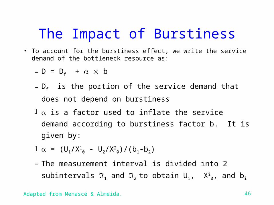
Adapted from Menascé & Almeida. 46
The Impact of Burstiness• To account for the burstiness effect, we write the service demand of
the bottleneck resource as:
– D = Df + b
– Df is the portion of the service demand that does not
depend on burstiness
is a factor used to inflate the service demand
according to burstiness factor b. It is given by:
= (U1/X10 - U2/X2
0)/(b1-b2)
– The measurement interval is divided into 2 subintervals
1 and 2 to obtain Ui, Xi0, and bi
Adapted from Menascé & Almeida. 47
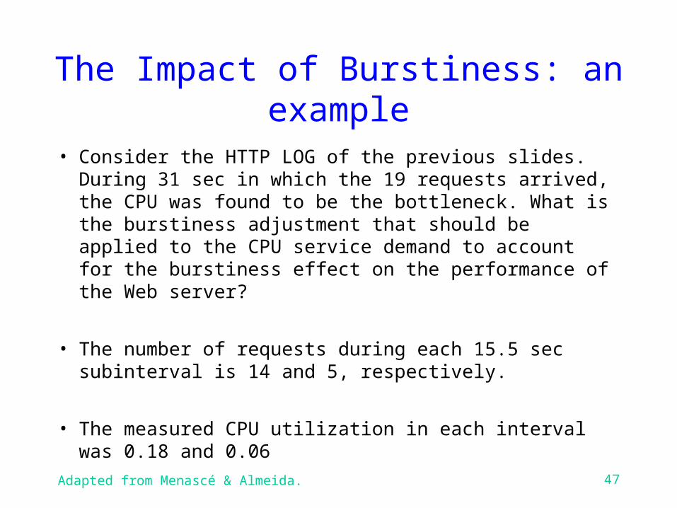
The Impact of Burstiness: an example
• Consider the HTTP LOG of the previous slides. During 31 sec in which the 19 requests arrived, the CPU was found to be the bottleneck. What is the burstiness adjustment that should be applied to the CPU service demand to account for the burstiness effect on the performance of the Web server?
• The number of requests during each 15.5 sec subinterval is 14 and 5, respectively.
• The measured CPU utilization in each interval was 0.18 and 0.06
Adapted from Menascé & Almeida. 48
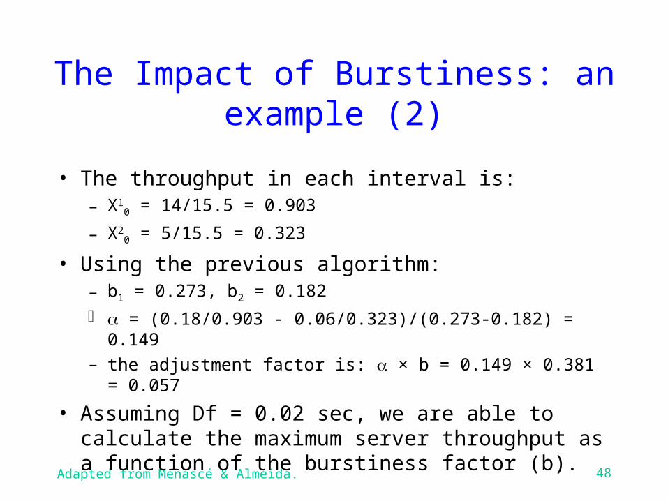
The Impact of Burstiness: an example (2)
• The throughput in each interval is:– X1
0 = 14/15.5 = 0.903
– X20 = 5/15.5 = 0.323
• Using the previous algorithm:– b1 = 0.273, b2 = 0.182
= (0.18/0.903 - 0.06/0.323)/(0.273-0.182) = 0.149– the adjustment factor is: × b = 0.149 × 0.381 = 0.057
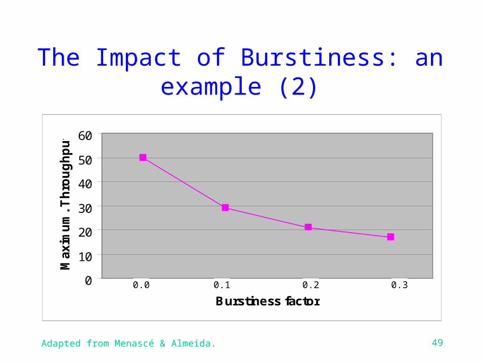
• Assuming Df = 0.02 sec, we are able to calculate the maximum server throughput as a function of the burstiness factor (b).
Adapted from Menascé & Almeida. 49
The Impact of Burstiness: an example (2)
0
10
20
30
40
50
60
Burstiness factor
Max
imu
m. T
hro
ug
hp
ut
0.30.10.0 0.2
Adapted from Menascé & Almeida. 50
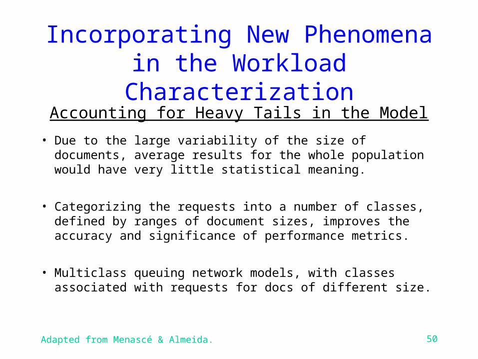
Incorporating New Phenomena in the Workload Characterization
Accounting for Heavy Tails in the Model
• Due to the large variability of the size of documents, average results for the whole population would have very little statistical meaning.
• Categorizing the requests into a number of classes, defined by ranges of document sizes, improves the accuracy and significance of performance metrics.
• Multiclass queuing network models, with classes associated with requests for docs of different size.
Adapted from Menascé & Almeida. 51
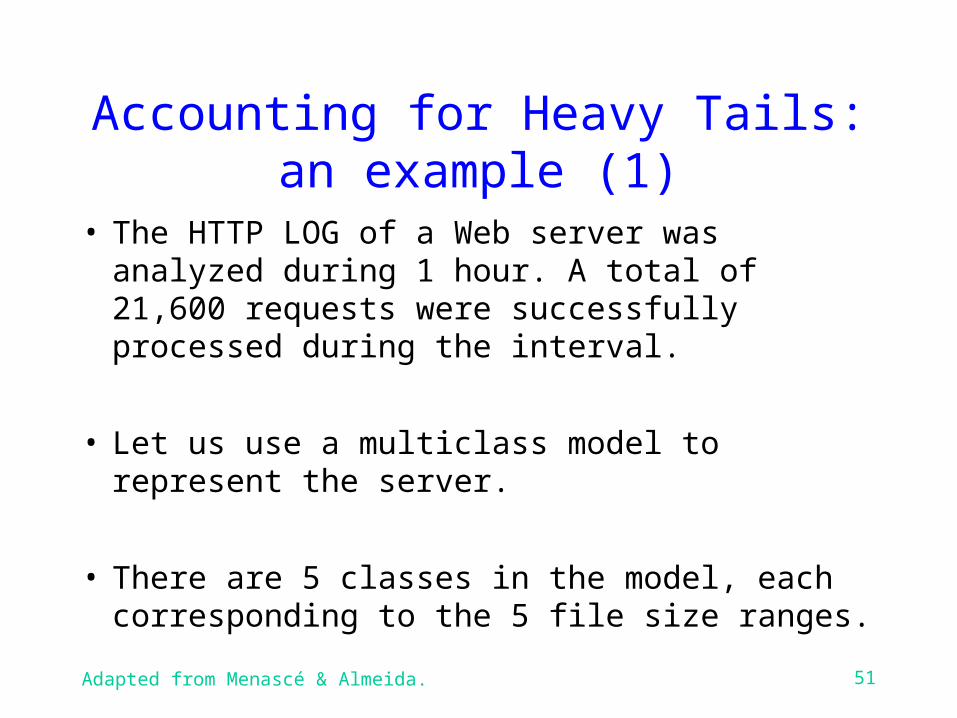
Accounting for Heavy Tails: an example (1)
• The HTTP LOG of a Web server was analyzed during 1 hour. A total of 21,600 requests were successfully processed during the interval.
• Let us use a multiclass model to represent the server.
• There are 5 classes in the model, each corresponding to the 5 file size ranges.
Adapted from Menascé & Almeida. 52
Accounting for Heavy Tails: an example (2)
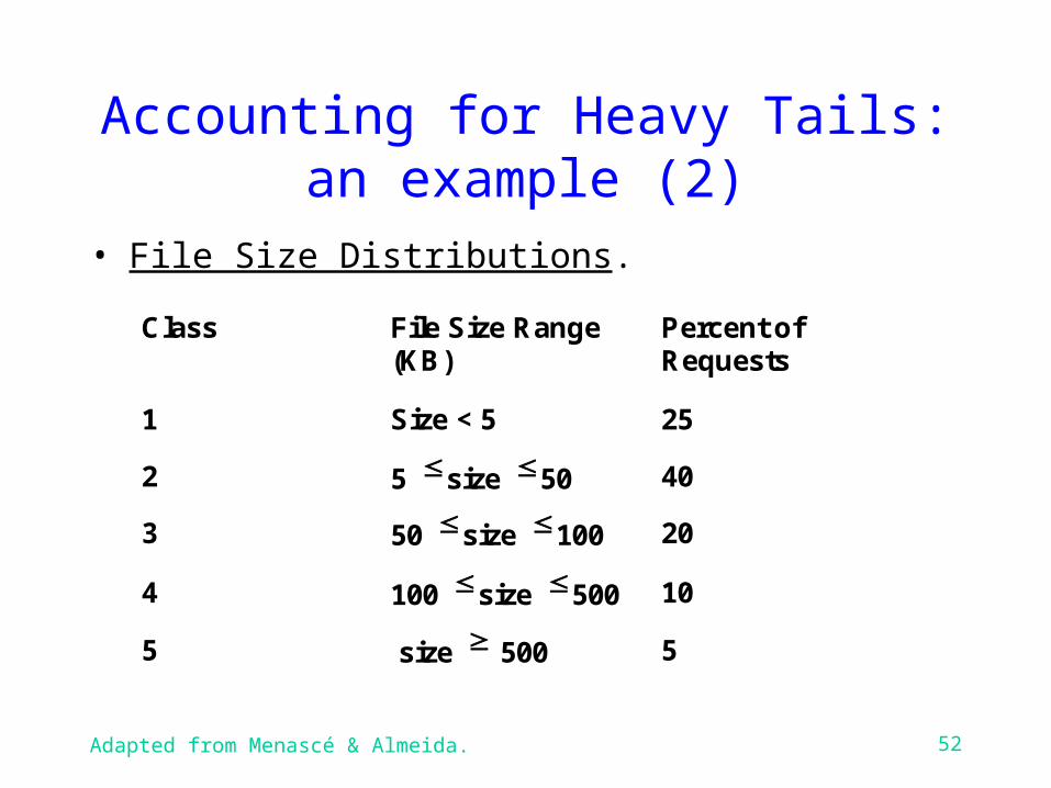
• File Size Distributions.
Class File Size Range(KB)
Percent ofRequests
1 Size < 5 25
2 5 size 50 40
3 50 size 100 20
4 100 size 500 10
5 size 500 5
Adapted from Menascé & Almeida. 53
Accounting for Heavy Tails: an example (3)
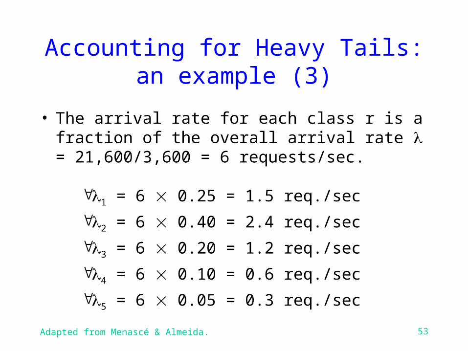
• The arrival rate for each class r is a fraction of the overall arrival rate = 21,600/3,600 = 6 requests/sec.
1 = 6 0.25 = 1.5 req./sec
2 = 6 0.40 = 2.4 req./sec
3 = 6 0.20 = 1.2 req./sec
4 = 6 0.10 = 0.6 req./sec
5 = 6 0.05 = 0.3 req./sec
Adapted from Menascé & Almeida. 54
Summary
� Workload Characterization� what is it?� basic concepts� workload description and modeling� representativeness of a workload model
� Methodology (1)� Choice of an analysis standpoint� Identification of the basic component� Choice of the characterizing parameters� Data collection
Adapted from Menascé & Almeida. 55
Summary
� Methodology (2)� Partitioning the workload� Calculating the class parameters
� Averaging
� Clustering techniques and algorithms
� New Phenomena in the Internet and WWW� Burstiness
� Heavy-tailed distributions