WORKING P A P E R

Gain and Loss Marriage and Wealth Changes Over Time

JULIE ZISSIMOPOULOS

WR-724

December 2009

This paper series made possible by the NIA funded RAND Center for the Study of Aging (P30AG012815) and the NICHD funded RAND Population Research Center (R24HD050906).

This product is part of the RAND Labor and Population working paper series. RAND working papers are intended to share researchers’ latest findings and to solicit informal peer review. They have been approved for circulation by RAND Labor and Population but have not been formally edited or peer reviewed. Unless otherwise indicated, working papers can be quoted and cited without permission of the author, provided the source is clearly referred to as a working paper. RAND’s publications do not necessarily reflect the opinions of its research clients and sponsors.

is a registered trademark.

Gain and Loss: Marriage and Wealth Changes Over Time

Julie M. Zissimopoulos, RAND

2009

Abstract

Family composition has changed dramatically over the past 25 years. Divorce

rates increased and remarriage rates declined. While considerable research established a link between marriage and earnings, far less is empirically understood about the effect of marriage on wealth although wealth is an important measure for older individuals because it represents resources available for consumption in retirement. In this paper we employ eight waves of panel data from the Health and Retirement Study to study the relationship between wealth changes and marital status among individuals over age 50. This research advances understanding of the relationship by first, incorporating measures of current and lifetime earnings, mortality risk and other characteristics that vary by marital status into models of wealth change; second, measuring the magnitude of wealth loss and gain associated with divorce, widowing and remarriage and third, estimating wealth change before and after marital status change so the change in wealth change is not the result of individuals entering or leaving the household and other sources of unobserved differences are removed from estimates of the effect of marriage on wealth. Our results suggest no differences in wealth change over time among individuals that remain married, divorced, widowed, never married and partnered over 7 years. In the short-run there are substantial wealth changes associated with marital status changes. Divorce at older ages is costly, remarriage is wealth enhancing and people appear to change their savings in response to changes in marital status. The research reported herein was pursuant to a grant from the U.S. Social Security Administration (SSA) funded as part of the Retirement Research Consortium (RRC). The findings and conclusions expressed are solely those of the authors and do not represent the views of SSA, any agency of the Federal Government or the RRC. I thank Joanna Carroll for her excellent programming assistance.

2

1. Introduction

Family composition has changed dramatically over the past 25 years. Divorce

rates rapidly increased from the late 1960’s through the 1980’s and remarriage rates have

declined (Cherlin 1992). Considerable research has established a correlation between

marital status and socio-economic status, particularly a positive relationship between

marriage and male earnings (Korenman and Neumark 1991; Lundberg and Rose 2002;

Loughran and Zissimopoulos 2009). Considerably less attention has been paid to the

effect of marriage on women’s earnings because of the strong correlation of marriage and

childbearing. One exception is Loughran and Zissimopoulos (2009) and they find

marriage lowers female wages the year of marriage and wage growth in subsequent years.

While income is a critical measure of well being, wealth is an important complementary

measure and arguably the most important measure for older individuals because it

represents resources available for consumption in retirement. Far less is empirically

understood about the effect of marriage on wealth compared to the effect of marriage on

earnings although theory suggests it is likely to be important.

An important implication of economic models of savings with no uncertainty (or

agents maximize expected utility) and perfect capital markets is that consumption is

determined by permanent income. This implies that changes in permanent income are

consumed and temporary changes are saved. Relaxing these assumptions provides a role

for both permanent and transitory income in consumption and savings decisions.

Changes in marital status that affect permanent income will change consumption levels.

Moreover, changes in marital status will affect wealth depending on whether the change

is considered transitory or permanent. For example, the behavioral response to a

3

separation or divorce expected to be temporary may be to lower savings to avoid a drop

in consumption. Lupton and Smith (2002) find dissaving is most common the shorter the

duration in the non-marriage state as households attempt to maintain prior consumption

levels. Consumption and savings behavior may change prior to the event. For example,

Zagorsky (2005) found that savings declines begin prior to divorce.

Other hypotheses regarding the effect of marriage on wealth include economies of

scale (Waite 1995), mortality risk (Lillard and Weiss 1996), children and inter-vivos

transfers and bequests (Hurd, Smith, Zissimopoulos 2006), precautionary savings

(Mincer 1978) and retirement planning. Married couples may consume many goods and

services jointly (entertainment, housing) for the same cost as a single person. These

economies of scale may translate into additional wealth or additional consumption.

Marriage may produce better health, thus married couples will save more to protect

against outliving their resources. On the other hand, marriage reduces risk associated with

fluctuations in income and thus may lower precautionary savings against income shocks

or other shocks.1 In sum, there are many pathways through which marriage and wealth

are associated. Moreover, the consistent empirical finding of a relationship between

marriage and wealth suggests its importance as an area for further study. Yet,

challenging estimation of the empirical relationship between marriage and wealth is the

non-random sorting of individuals into marriage. For example, low-income families are

more likely to divorce or experience widowhood than high-income families. Prior

empirical studies have been hindered by a lack of control measures for permanent income

1 Children are one important reason for marriage and their presence may either increase savings (to leave as a bequest) or decrease savings because of the additional consumption associated with children.

4

and by use of cross-sectional surveys and short panels that are ill-suited for distinguishing

between selection and behavioral response.

In this paper we employ eight waves of panel data from the Health and

Retirement Study to study the relationship between wealth changes and marital status

among individuals over age 50. This research advances understanding of the relationship

by first, incorporating measures of current and lifetime earnings, mortality risk and other

characteristics that vary by marital status into models of wealth change; second,

measuring the magnitude of wealth loss and gain associated with divorce, widowing and

remarriage and third, estimating wealth change before and after marital status change so

the change in wealth change is not the result of individuals entering or leaving the

household and other sources of unobserved differences are removed from estimates of the

effect of marital status on wealth. The remainder of this paper has the following structure.

The next section summarizes describes the data and derivation of key variables. Section

3 presents main results for wealth levels and changes and for individuals that do and do

not change marital status. The final section concludes.

2. Data

The research relies on longitudinal data from the Health and Retirement

Study, a set of biennial surveys first fielded in 1992 and 1993 by the University of

Michigan with the objective to monitor economic transitions in work, income and wealth,

and changes in health among those over 50 years old.2 We use data from survey waves

1992, 1993, 1994, 1995, 1996 and biennial thereafter to 2006.3

2 The first survey, the Health and Retirement Study (HRS) began as a national sample of about 7,600 households (12,654 individuals) with at least one person in the birth cohorts of 1931 through 1941 (about

5

We use data including all cohorts with the exception of the 1948 to 1953 birth

cohort added in year 2004 for which insufficient waves of data for this analysis have been

collected. In addition, we use restricted data on Social Security earnings to compute a

measure of lifetime earnings. Marital history variables (all prior marriages, divorces and

widowings) were derived based on the raw HRS files; most other variables used in the

study are from the RAND HRS Data file, Version I4. Further details on key analytic

variables follow.

Marital Status. Respondents are categorized at a point in time as being either

married, divorced, widowed, partnered or never married. For some analyses we use

respondents’ reports of past marital events to distinguish between married and remarried

individuals. Changes over the panel are based on respondents’ report of any changes

between waves and we group them into six categories: separated to divorced, married to

divorced, married to widowed, divorced to married, widowed to married, other single

(partnered or never married) to married.

Lifetime Earnings. We calculate lifetime earnings based on historical earnings

reported to the Social Security Administration. We use earnings from 1951 to 1991 for

9,539 HRS respondents.5 Earnings data for the War Babies cohort are available for 1,330

51-61 years old at the wave 1 interview in 1992). The second, the Assets and Health Dynamics of the Oldest Old (AHEAD), began in 1993 and included 6,052 households (8,222 individuals) with at least one person born in 1923 or earlier (70 or over in 1993). In 1998, HRS was augmented with baseline interviews from at least one household member from the birth cohorts 1924-1930 and 1942-1947 and was representative of all birth cohorts born in 1947 or earlier. In 2004, the HRS was again augmented with interviews from the birth cohort 1948-1953. 3 For the original HRS respondents from survey wave 1992, we use a total of 8 waves of data from 1992 to 2006. For the original AHEAD respondents from 1993, we have 7 waves of data. For respondents added in 1998, we have 5 survey waves from 1998 to 2006. 4 RAND HRS is a longitudinal data set based on the HRS data and developed at RAND with funding from the National Institute on Aging and the Social Security Administration. 5 See Haider and Solon (2000) for a discussion of characteristics of individuals with and without matched Social Security records.

6

respondents for years 1951 to 1997. The administrative records are accurate and less

subject to measurement error than self-reported earnings from household surveys and

cover a long history of earnings. They are however, limited in two ways. First, the level

of earnings is reported only up to the Social Security maximum. This maximum changed

over time as did the number of individuals whose earnings were above the maximum.

Second, individuals employed in a sector not covered by Social Security have no earnings

records for the years he or she is employed in the uncovered sector.6 Lifetime earnings

are calculated as the present discounted value (3 percent real interest rate) of real Social

Security earnings adjusted to 2006 dollars using the CPI-U-RS, and we adjust for the

upper truncation of Social Security earnings.

Mortality Risk, Risk Aversion, Time Rate of Preference. Mortality risk is the

respondent’s subjective survival assessment of living to age 75 (85) on a zero to 100

scale and we include it in empirical models as the deviation from lifetables based on sex

and age. The basis for categorizing the level of risk aversion is a series of questions that

ask respondents to choose between pairs of jobs where one job guarantees current family

income and the other offers the chance to increase income and carries the risk of loss of

income. From responses to these questions we categorize a respondent’s level of risk

aversion into four groups. We measure respondents’ time rate of preference by their

responses to the length of time they use for financial planning. The answers are

categorical from a few months to over ten or more years.

Wealth. Our main outcome measures are wealth, change in wealth and the change

in the change in wealth. Wealth is housing plus non-housing wealth and is computed as

the sum of wealth from real estate, businesses, IRAs, stocks, bonds, checking accounts, 6 In 1996, 92% of non-self-employed wage and salary workers were covered by Social Security.

7

CDs, and housing, less the value of the mortgage, home loans, and other debt. Missing

data on wealth are imputed and the methods are described in RAND HRS Version I.

Some analysis use information on a respondent’s pension ownership and type (defined

benefit, defined contribution, both).

3. Results

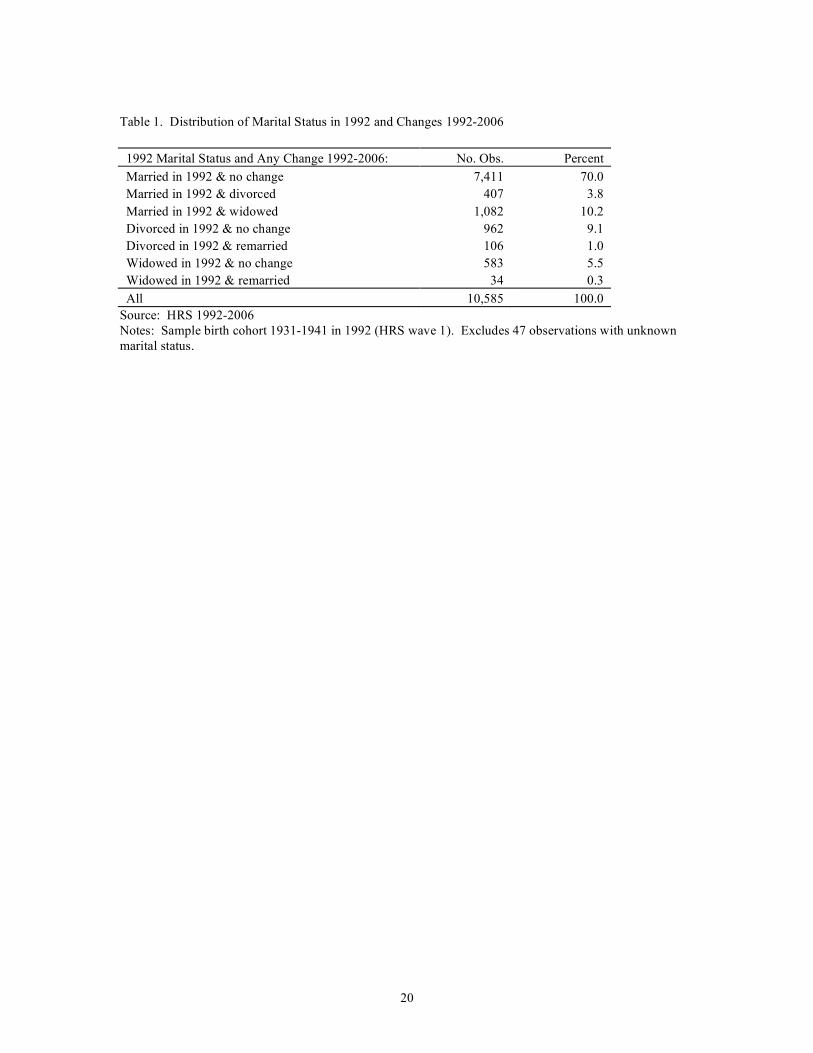
Changes in marital status occur over the lifespan, even at older ages. We

examine current marital status and future changes in marital status over the next 14 years

and present their distribution in Table 1. Among the birth cohort 1931-1941, 84 percent

are married in 1992, 10 percent are divorced and 6 percent are widowed. Over the next 14

years, 15 percent of this sample of respondents, on average 55 years old, change marital

status. About 4 percent of married respondents divorce and 10 percent are widowed.

Just over one percent of individuals divorced or widowed remarries over this time period.

The level of wealth held in 1992 by this birth cohort varies with current marital

status as well as future changes in marital status. The first three rows in Table 2 are

groups that, as of 1992, have not experienced a marital disruption. The data in Table 2

shows respondents that are married in 1992 and have no marital status changes over the

next 14 years have higher mean and median wealth than married respondents that will

eventually divorce or be widowed. This group of continuously married individuals has

on average $363,814 in housing and non-housing wealth (not including pension wealth)

compared to $278,365 for married respondents that will divorce and compared to

$254,362 for married respondents that will be widowed. Age differences by group are

small and thus unlikely to account for the mean and median differences. Remarried

8

individuals that remain married through the 14 years have lower average wealth

($281,843) than married individuals who remain married over the panel, and at the mean

and median, only marginally higher than those married that will go on to divorce or be

widowed. All not married individuals have lower mean wealth than married individuals

although at the median, not married individuals who remarry in panel have higher median

wealth than some married individuals. Among the not married groups, mean wealth of

divorced ($116,572) and widowed ($125,835) individuals that remain not married is

about 60% of the wealth that not married individuals that go on to remarry have

($188,366 and $199,769 respectively for divorced then remarried and widowed and then

remarried).

The wealth differences at about age 55 by current marital status and future

changes may be a result of wealth loss due to marital disruption or observable differences

in for example, earnings or preferences for savings. For example, marital groups may

save at similar rates but save out of lower levels of income. Table 2 also shows lifetime

earnings, current earnings and the ratio of wealth to lifetime earnings. Comparing

individuals that are married and stay married with those that are married and go on to

divorce, Table 2 shows that lifetime earnings and current earnings are similar and thus

differences in earnings over the life-cycle is unlikely to account for the wealth

differences. Remarried individuals that stay remarried have slightly higher lifetime

earnings, same current earnings and yet, their mean wealth is 77 percent of the wealth of

individuals that are married (not remarried) and stay married over the panel. This is

pattern is consistent with wealth loss due to marital disruption. Not married individuals

have lower wealth than married individuals and indeed, their lifetime and current

9

earnings are lower than married individuals. In sum, these data in Table 2 emphasize the

role of lifetime earnings, the role of selection on characteristics other than income and the

role of wealth loss due to marital dissolution in explaining wealth level differences by

marital status.

Changes in wealth among individuals with stable marital status.

The magnitude of wealth change over time among individuals that change marital

status will be dominated by wealth change due to individuals leaving or entering the

household. Thus we first examine wealth changes over two years (all data waves (t) and

(t+1)) for individuals that do not change marital status over that same time period and

results are shown in Table 3.7 Wealth increases over two years for all groups. Married

and remarried individuals have larger wealth changes than divorced, widowed, never

married and partnered individuals. Compared to all other individuals wealth change is

higher for married individuals by the following amounts: $3,222 compared to remarried,

$10,142 compared to divorced, $17,317 compared to widowed, $11,627 compared to

never married and $17,115 compared to partnered. Wealth change as a percent of initial

wealth level is slightly higher for divorced individuals (9 percent) than married,

remarried and never married (7 percent). Wealth change as a percent of initial wealth

level is 3 percent among widowed and partnered individuals. Thus, overall levels of

wealth change are highest for married individuals but rates are similar compared to

divorced and never married individuals.

7 We trim the top and bottom 2 percent of wealth change values.

10

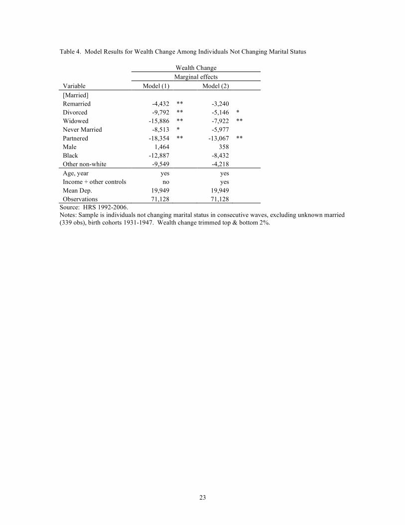
We examine two-year wealth change by marital status controlling for basic

demographic differences in sex, race and age and including year indicators. Results from

the linear, multivariate model are reported in the first column of results in Table 4 (Model

1). The second column of results in Table 4 (Model 2) are estimates of the marginal

effects of marital status on wealth change over two-years from a model that along with

basic demographics, includes in the specification many other covariates including

lifetime earnings (a measure of permanent income), current earnings, education, number

of children, ownership of pension wealth and type of pension, mortality risk, risk

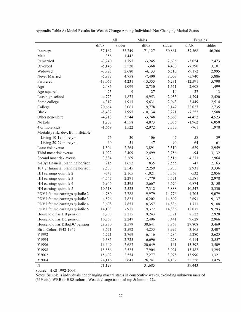
aversion, and financial planning horizon. The marginal effects for all covariates are

given in Appendix Table A. The results from Model 1 show remarried and all not

married individuals have lower levels of wealth change over two years and the magnitude

of difference is similar to the difference in Table 3. The inclusion of the additional

covariates (Model 2) explains all of the difference in wealth change between married and

remarried individual. The covariates reduce the difference in wealth change between

married and remarried in Model 1 and Model 2 by $1,192 (27 percent) and the difference

is no longer statistically significant. The additional covariates in Model 2 explain about

50% of the wealth change difference between married and either divorced or widowed

individuals. That is, the marginal effect is reduced from $-9,792 in Model 1 to $-5,146 in

Model 2 for divorced individuals and from $-15,886 to $-7,922 for widowed individuals.

The additional covariates in Model 2 explain about 30% of the wealth change difference

between married and either never married or partnered individuals. Overall, measures of

socio-economic status (lifetime and current earnings, education), pensions, and mortality

11

risk explain between 30 and 50 percent of the difference in wealth between married and

not married individuals.

Table 5 presents results for the effect of marital status on wealth change

separately for samples of men and women. For men, demographic characteristics

(included in Model 1) explain all of the difference in wealth change between married,

remarried and not married men with the exception of partnered men. The inclusion of the

additional covariates in Model 2 explains about 30 percent of the difference between

married men and partnered men. For women, wealth change is lower for remarried and

all not married women compared to married women with the exception of never married

women. The inclusion of the additional covariates in Model 2 explains all of the

difference between married and remarried or never married women, 40 percent of the

difference between married and divorced women, 49 percent of the difference between

married and widowed women and 30 percent of the difference between partnered and

married women.

In sum, basic demographics explain all of the difference in wealth change by

marital status for men (exception is partnered men), but not so for women. For women,

the inclusion of additional controls for socio-economic status and other household and

individual characteristics explains all of the difference between married and remarried

women and between one third and one half of the difference between married women and

other not married women. Thus for women, some of the variation is left unexplained.

Changes in wealth among individuals that change marital status.

12

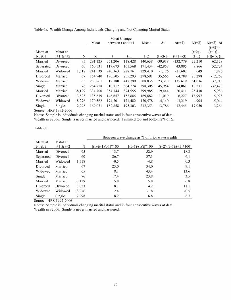
To study wealth change in panel among individuals that change marital status, we

examine wealth levels and changes in the two waves prior to the marital status change (t-

1 and t), the two years over which the marital status change occurred (t and t+1) and the

two years after the marital status change occurred (t+1 and t+2). Thus we limit our

sample to individuals in four consecutive waves of data and exclude individuals with

more than one marital change between survey waves.8 We also study wealth changes

over the same time periods for individuals that do not change marital status. Results on

wealth levels and changes are given in Table 6a and wealth changes as a percentage of

the prior wave wealth level in Table 6b.

Among married and separated individuals that divorce between waves, wealth is

already declining in the wave prior to the divorce (Table 6a). Married individuals that are

divorced in time t+1 experienced a $39,918 wealth loss while married from time (t-1) to

(t), or 14 percent of their time (t-1) wealth (Table 6b). Over the two years in which the

divorced occurred, married individuals lost another $132,779 in wealth or about 53

percent of their time (t) wealth. There is some wealth recovery after the divorce: wealth

increased by $22,210 or 19 percent. The dissaving before the divorce and savings after

the divorce lead to a wealth change of $62,128 from before ((t-1) to (t)), to after ((t+2)-

(t+1)) the divorce. Separated individuals have wealth declines of $42,858 over the two

years they are separated ((t)-(t-1)) and prior to the divorce, which is 27 percent of their

time (t-1) wealth. Unlike married couples that divorce, separated individuals have wealth

increases during the wave in which they divorce and the wave in which they are divorced.

8 We analyze characteristics of this sample restricted to be in four consecutive waves and find no statistically significant differences in average age, education, number of children, mean and median wealth or earnings. Although the differences are not statistically different, the sample in four consecutive waves has slightly higher wealth and earnings.

13

Wealth change is positive for all groups that change marital status, after the

change. In fact, the wealth change from t+1 to t+2 for married to divorced, divorced to

married and married to married is similar and is between $22,000 and $25,000 but

represents a larger percentage of wealth for divorced individuals who went from married

to divorced. The wealth change experience of married individuals who are widowed

between time (t) and (t+1) is much different than those who divorced. There is no

significant wealth loss in the years before the widowing occurred, the widowing results in

a wealth decline of $11,602 over two years or about 5 percent of their married (pre-

widowed) wealth at time (t).

Divorced individuals that remarry accumulate assets while divorced (change (t-1)

to (t) is $35,565) at a higher level and rate than those who remain divorced ($11,019).

Assets enter the household with marriage: wealth levels increase $64,789 between waves

that individuals go from divorced to married and then level back to levels and rates

similar to those individuals who remain married. Widow and other singles (never

married and partners) that marry also show substantial increases in wealth over the waves

in which they get married and then a smaller increase in (in level and rate) the following

waves in which they are married.

In sum, divorce is associated with wealth loss and the loss in wealth begins before

the divorce occurs and wealth recovery in the form of increased savings after the divorce.

In contrast, a widowing is associated with much a smaller magnitude of wealth loss.

Remarriage and marriage (for never married) is associated with increases in wealth at the

time of remarriage consistent with the addition of an individual bringing wealth into the

household followed by future wealth increases of lower levels.

14

Empirical models of the change in the change in wealth

Demographic controls, measure of lifetime and current earnings and other rich

measures of characteristics accounted for all of the differences in wealth change by

marital status among men (exception is partnered men) and some of the difference among

women for samples of individuals that did not change marital status. If there is remaining

unobserved heterogeneity correlated with marital status then the marginal effects of

marital status on wealth change will be biased. We eliminate unobserved heterogeneity

fixed over time (e.g. prudence) and measure the effect of marital status and changes in

income growth with additional controls for age and year by estimating models of the

change in wealth change. We estimate wealth change for individuals that change marital

status, before and after the marital status change so measured wealth change is not

primarily the result of individuals entering or leaving the household. That is, we use

change in wealth change [(t+2)-(t+1)] – [(t)-(t-1)] and the change ((t+1)-(t)) is the wave

in which marital status changed and is omitted from the calculation.

Our model of the change in wealth change, for a sample of respondents that are

present in 4 consecutive waves, includes all possible marital statuses (excluded is

married, no change over time), change in the change in income over this same time

period, age, sex and year indicators.9 Estimation results are given in Table 7 for all

respondents and separately for males and females. The top and bottom 2 percent of the

dependent variable (change in wealth change) is trimmed. If there is no change in

savings behavior, we would expect the change in the change to be small. The mean 9 We include all respondents from birth cohorts 1947 or earlier. Restricting the sample to respondents in the 1931-1941 and 1942-1947 cohorts as we do in the model with results shown in Tables 4 and 5 does not change our findings.

15

dependent variable is $4,188. We discuss the findings noting that the standard errors

around most estimates are large so few statistically differences are found.

Consistent with our earlier findings from models of wealth change on a sample of

individuals that do not change marital status, the magnitude of effect of marital status on

the change in wealth change among individuals that remain divorced, widowed or single

over the four waves is small and not different than for individuals that remain married.

For example the change in wealth change is $912 less among divorced individuals

compared to married individuals and $3,266 less for widows compared to married

individuals (Table 7). The difference in the change in wealth change between widows

and married individuals decrease from the mean difference (Table 6a) once age controls

are added. Among women, there is no difference in the change in wealth change of

women that stay divorced, widowed or other single women over the four waves

(partnered or never married) compared to married women that remain married.

The marginal effects on marital status changes from married or separated to

divorced or widowed are positive suggesting transition to a not married state is leading to

higher savings relative to the change in savings of married couples. As we saw in Table

6a, the large positive change in wealth change is due to dissaving that occurs in the waves

before the wave in which the divorce occurs and the ‘recovery’ of savings in the divorced

state. The inclusion of the change in income change does reduce the magnitude from

those reported in Table 6a. Individuals that divorce from a married state have a change in

wealth change that is $46,858 higher than individuals that remain married. The difference

in the change in wealth change between married individuals that divorce and those that

remain married is decreased by $15,270 from the mean difference ($62,128 in Table 6a)

16

once controls are added. This estimate is lower for men ($41,494) than women ($50,478).

Married individuals that are widowed have a slightly higher change in savings compared

to individuals that remain married ($3,494). Widowed men have a small decline in

savings and women a small increase relative to men and women that remain married.

Divorced individuals that remarry have a change in savings that is less ($-17,606)

than individuals that remain married. Widowed men and women that marry have a

change in wealth change that is more ($31,907) than individuals that remain married.

The estimates are imprecisely measured and the inclusion of change in income change

and age does not change the magnitude of the difference relative to married couples

reported in Table 6a. The effects are different for men and women. For divorced and

widowed women, remarriage leads to a higher change in wealth change than married

women while for men it leads to a lower change.

Change in savings is declining with age slowly ($-539) but more rapidly for men

($-712) than women ($-444). Savings increases with the change in income growth. For

example, a $1,000 increase in income growth (change in change in income) increases the

change in wealth change by $208 ($241 and $191 for men and women respectively).

We interpret these findings cautiously. Model estimates of the effects of marital

status on change in wealth change are imprecisely measured. Moreover, the estimates on

individuals that change marital status are based on short-term changes – changes in

savings behavior immediately before and after a marital status event and not reflecting

long-term savings behavior. Indeed we find no difference in the change in wealth change

between individuals that remain divorced, widowed or single and married over the four

waves of data. Finally, throughout this analysis we measure wealth change and not active

17

savings. That is, wealth change will include capital gains or losses and other transfers

into the household through mechanisms such as pension and inheritance but not through

the marital transition itself.

4. Conclusion

By comparing wealth levels and lifetime earnings at age 55 of married and

remarried individuals by whether they go on to divorce over the next 14 years or not, we

found patterns consistent with the role of both selection and wealth loss due to marital

dissolution in explaining why married individuals around age 55 have higher wealth than

not married individuals. Among individuals with a stable marital status over time, we

find the higher savings of couples compared to not married men (except partners) is

accounted for by observable differences in economic status, pensions and mortality risk.

Observable differences account for between a third and one-half of the mean savings

differences between married and divorced, widowed and partnered women and all of the

difference between couples and never married women. Estimates from models that

control for fixed and unobserved heterogeneity by modeling the change in wealth change

reveal no difference in the change in wealth change for men and women that are not

married consistently over four waves compared to men and women married consistently

over four consecutive waves. There is wealth change associated with changes in marital

status. Divorce is associated with wealth loss beginning while married - between four

and two years before the divorce occurs- substantially more wealth loss over the two

years that the individual transitions from married to divorced, and wealth recovery in the

form of increased savings after the divorce. Remarriage is associated with increases in

18

wealth at the time of marriage consistent with the addition of an individual bringing

wealth into the household and followed by future wealth increases at rates similar to

those who do not change marital status. Divorce at older ages is costly and remarriage is

wealth enhancing and people appear to respond to marital status changes by changing

their savings behavior.

19

References Cherlin, A. 1992. Marriage, Divorce and Remarriage. Cambridge, MA: Harvard

University Press. Haider, Steven and Gary Solon. 2000. Non-Response Bias in the HRS Social Security

Files. RAND Working Paper DRU-2254-NIA, February. Korenman, Sanders and David Neumark. 1991. Does Marriage Really Make Men More

Productive? The Journal of Human Resources 26(2): 282-307. Lillard, Lee and Yoram Weiss. 1996. Uncertain Health and Survival: Effect on End-of-

Life Consumption. Journal of Business and Economic Statistics 15(2): 254-68. Loughran, David and Julie Zissimopoulos. 2009. Why Wait? The Effect of Marriage

and Childbearing on the Wage Growth of Men and Women. The Journal of Human Resources 44(2): 326-349.

Lundberg, Shelly and Elaina Rose. 2002. The Effects of Sons and Daughters on Men's

Labor Supply and Wages. Review of Economics and Statistics 84(2): 251-68. Lupton, Joseph and James Smith 200). ‘Marriage, Assets and Savings’, 129–52 in

Shoshana Grossbard-Shechtman (ed.) Marriage and the Economy: Theory and Evidence from Advanced Industrial Societies. New York and Cambridge: Cambridge University Press.

Mincer, Jacob. 1978. Family Migration Decisions. The Journal of Political Economy

86(5): 749-773. Waite, Linda. 1995. Does Marriage Matter? Demography 32(4): 483-507. Zagorsky, Jay. 2005. Marriage and divorce’s impact on wealth. Journal of Sociology

41(4): 406–424.

20

Table 1. Distribution of Marital Status in 1992 and Changes 1992-2006

1992 Marital Status and Any Change 1992-2006: No. Obs. Percent Married in 1992 & no change 7,411 70.0 Married in 1992 & divorced 407 3.8 Married in 1992 & widowed 1,082 10.2 Divorced in 1992 & no change 962 9.1 Divorced in 1992 & remarried 106 1.0 Widowed in 1992 & no change 583 5.5 Widowed in 1992 & remarried 34 0.3 All 10,585 100.0

Source: HRS 1992-2006 Notes: Sample birth cohort 1931-1941 in 1992 (HRS wave 1). Excludes 47 observations with unknown marital status.

21

Table 2. Wealth, Lifetime and Current Earnings in 1992 by Marital Status in 1992 and Changes 1992-2006 Median Mean Ratio N Wealth Wealth LTE Earnings Wealth/LTE Married in 1992 & no change 5,472 173,457 363,814 1,241,020 57,201 0.293 Married in 1992 & divorced 204 99,919 278,365 1,026,509 60,821 0.271 Married in 1992 & widowed 760 121,618 254,362 923,538 37,259 0.275 Remarried in 1992 & no change 1939 125,311 281,843 1,346,968 57,668 0.209 Remarried in 1992 & divorced 203 85,080 232,421 1,215,924 46,496 0.191 Remarried in 1992 & ever widowed 322 98,271 201,530 1,021,238 35,652 0.197 Divorced in 1992 & no change 962 33,175 116,572 636,788 24,444 0.183 Divorced in 1992 & ever remarried 106 105,525 188,366 888,625 42,503 0.212 Widowed in 1992 & no change 583 47,684 125,835 403,610 14,904 0.312 Widowed in 1992 & ever remarried 34 129,137 199,769 521,556 26,421 0.383 All 10585 129,928 293,975 1,127,296 49,511 0.261

Source: HRS 1992-2006 Notes: Sample birth cohort 1931-1941 in 1992 (HRS wave 1). Excludes 47 observations with unknown marital status. Wealth reported in $2006. LTE is lifetime earnings.

22

Table 3. Wealth Change Over 2 Years Among Individuals with No Change in Marital Status Mean

N (t) (t+1) ∆ =(t+1)-(t) ∆ as % of

wealth at (t) Married 51,444 349,951 372,545 22,595 6.5 Remarried 17,576 285,050 304,423 19,373 6.8 Divorced 8,321 136,889 149,342 12,453 9.1 Widowed 19,358 161,955 167,234 5,278 3.3 Never Married 2,928 155,061 166,029 10,968 7.1 Partnered 2,315 206,856 212,337 5,480 2.6 All 101,942 276,824 294,024 17,200 6.2

Source: HRS 1992-2006 Notes: Sample individuals not changing marital status over two waves of data. Wealth in $2006.

23

Table 4. Model Results for Wealth Change Among Individuals Not Changing Marital Status Wealth Change Marginal effects Variable Model (1) Model (2) [Married] Remarried -4,432 ** -3,240 Divorced -9,792 ** -5,146 * Widowed -15,886 ** -7,922 ** Never Married -8,513 * -5,977 Partnered -18,354 ** -13,067 ** Male 1,464 358 Black -12,887 -8,432 Other non-white -9,549 -4,218 Age, year yes yes Income + other controls no yes Mean Dep. 19,949 19,949 Observations 71,128 71,128

Source: HRS 1992-2006. Notes: Sample is individuals not changing marital status in consecutive waves, excluding unknown married (339 obs), birth cohorts 1931-1947. Wealth change trimmed top & bottom 2%.

24

Table 5. Model Results for Wealth Change Among Individuals Not Changing Marital Status By Sex Wealth Change Men Women Marginal effects Marginal effects Model (1) Model (2) Model (1) Model (2) [Married] Remarried -4,012 -3,245 -4,806 * -3,054 Divorced -5,136 -368 -12,397 ** -7,390 * Widowed -8,227 -4,133 -17,948 ** -9,172 ** Never Married -8,128 -7,400 -9,174 -5,740 Partnered -18,825 ** -13,355 * -17,824 ** -12,591 * Black -15,232 -10,134 -11,210 -7,252 Other non-white -9,968 -3,748 -9,087 -4,452 Age, year yes yes yes yes Income + controls no yes no yes Mean Dep. 21,986 21,986 18,312 18,312 Observations 31,685 31,685 39,443 39,443

Source: HRS 1992-2006. Notes: Sample is individuals not changing marital status in consecutive waves, excluding unknown married (339 obs), birth cohorts 1931-1947. Wealth change trimmed top & bottom 2%

25

Table 6a. Wealth Change Among Individuals Changing and Not Changing Marital Status

Mstat Mstat Change

between t and t+1 Mstat Δt Δ(t+1) Δ(t+2)

Δ(t+2) -Δt

Mstat at t-1 & t

Mstat at t+1 & t+2 N t-1 t t+1 t+2 (t)-(t-1) (t+1) -(t)

(t+2) -(t+1)

[(t+2) -(t+1)] –

[(t)-(t-1)] Married Divorced 95 291,125 251,206 118,428 140,638 -39,918 -132,779 22,210 62,128 Separated Divorced 60 160,531 117,673 161,568 171,434 -42,858 43,895 9,866 52,724 Married Widowed 1,518 241,539 240,363 228,761 229,410 -1,176 -11,602 649 1,826 Divorced Married 67 154,940 190,505 255,293 278,591 35,565 64,789 23,298 -12,267 Widowed Married 65 288,861 312,180 447,799 508,835 23,318 135,619 61,036 37,718 Single Married 76 264,758 310,712 384,774 398,305 45,954 74,061 13,531 -32,423 Married Married 38,129 334,700 354,144 374,555 399,985 19,444 20,411 25,430 5,986 Divorced Divorced 3,823 135,639 146,657 152,885 169,882 11,019 6,227 16,997 5,978 Widowed Widowed 8,276 170,562 174,701 171,482 170,578 4,140 -3,219 -904 -5,044 Single Single 2,298 169,071 182,858 195,303 212,353 13,786 12,445 17,050 3,264

Source: HRS 1992-2006 Notes: Sample is individuals changing marital status and in four consecutive waves of data. Wealth in $2006. Single is never married and partnered. Trimmed top and bottom 2% of Δ. Table 6b. Between wave change as % of prior wave wealth Mstat at t-1 & t

Mstat at t+1 & t+2 N [(t)-(t-1)/t-1]*100 [(t+1)-(t)/t]*100 [(t+2)-(t+1)/t+1]*100

Married Divorced 95 -13.7 -52.9 18.8 Separated Divorced 60 -26.7 37.3 6.1 Married Widowed 1,518 -0.5 -4.8 0.3 Divorced Married 67 23.0 34.0 9.1 Widowed Married 65 8.1 43.4 13.6 Single Married 76 17.4 23.8 3.5 Married Married 38,129 5.8 5.8 6.8 Divorced Divorced 3,823 8.1 4.2 11.1 Widowed Widowed 8,276 2.4 -1.8 -0.5 Single Single 2,298 8.2 6.8 8.7

Source: HRS 1992-2006 Notes: Sample is individuals changing marital status and in four consecutive waves of data. Wealth in $2006. Single is never married and partnered.

26

Table 7. Model of Change in Wealth Change Before (t)-(t-1) and After (t+2)-(t+1) Marital Status Change Total Wealth ((t+2)-(t+1)) – ((t)-(t-1)) Marginal Effects All stderr Male stderr Female stderr Intercept 29,660 9,686 42,263 17,152 23,008 11,725 Marital Status in (t) & (t-1):

Marital Status (t+2) & (t+1):

[Married] [Married] Divorced Divorced -912 4,981 -4,415 9,432 1,098 5,806 Widowed Widowed -3,266 4,040 -4,175 9,795 -3,049 4,598 Other Single Other Single -1,963 6,270 -1,214 9,988 -2,807 8,051 Married Divorced 46,858 29,986 41,494 48,045 50,478 38,265 Separated Divorced 46,828 37,706 72,508 64,724 31,900 46,002 Married Widowed 3,494 7,772 -2,844 15,933 5,058 8,760 Divorced Married -17,606 35,677 -54,418 48,631 33,944 53,570 Widowed Married 31,907 36,224 -9,202 56,381 65,841 47,262 Other Single Married -40,975 33,526 -53,532 49,289 -26,563 46,017 Age -539 145 -712 254 -444 181 Male 730 2,641 Income change ((t+2)-(t+1)) – ((t)-(t-1)) 0.208 0.011 0.241 0.020 0.191 0.014 Four consecutive data waves are: 1992/93, 1994/95, 1996, and 1998 7,621 3,724 9,767 6,036 6,147 4,716 1994/1995, 1996, 1998, and 2000 27,184 4,300 28,725 6,773 25,982 5,570 1996, 1998, 2000 and 2002 -16,883 3,866 -21,953 6,273 -13,277 4,889 2000, 2002, 2004 and 2006 34,785 3,745 39,111 6,084 31,771 4,732 Mean Dependent 4,188 5,774 3,058 Observations 54,407 22,629 31778 Source: HRS 1992-2006. Notes: Sample is individuals in four consecutive waves, excluding unknown married (339 obs), birth 1947 and earlier. Dependent variable, ‘change in wealth change’ excludes wealth changes between the waves in which the marital transitions occurs (t and t+1) and values in the top & bottom 2% are trimmed. Age is measured at time (t).

27

Appendix Table A: Model Results for Wealth Change Among Individuals Not Changing Marital Status All Males Females df/dx stdder df/dx stdder df/dx stdder Intercept -57,162 33,749 -71,127 50,861 -57,368 46,266 Male 358 1,442 Remarried -3,240 1,795 -3,245 2,636 -3,054 2,473 Divorced -5,146 2,520 -368 4,430 -7,390 3,101 Widowed -7,923 2,680 -4,133 6,510 -9,172 2,995 Never Married -5,977 4,758 -7,400 8,007 -5,740 5,886 Partnered -13,067 4,231 -13,355 6,231 -12,591 5,790 Age 2,486 1,099 2,730 1,651 2,608 1,499 Age-squared -25 9 -27 14 -27 13 Less high school -4,773 1,873 -4,953 2,953 -4,794 2,420 Some college 4,317 1,913 5,631 2,943 3,449 2,514 College 20,664 2,063 19,778 3,147 22,027 2,735 Black -8,432 1,995 -10,134 3,271 -7,252 2,508 Other non-white -4,218 3,544 -3,748 5,668 -4,452 4,523 No kids 1,237 4,558 4,873 7,086 -1,962 6,058 4 or more kids -1,669 1,522 -2,972 2,373 -761 1,978 Mortality risk: dev. from lifetable:

Living 10-19 more yrs 76 30 106 47 58 39 Living 20-29 more yrs 60 51 47 90 64 61

Least risk averse 1,504 2,264 3,891 3,510 -629 2,959 Third most risk averse 1,022 2,409 2,499 3,756 -94 3,132 Second most risk averse 3,834 2,269 3,311 3,516 4,273 2,964 5-10yr financial planning horizon 215 1,652 835 2,555 -47 2,163 10+ yr financial planning horizon 2,538 2,545 2,259 3,933 2,931 3,336 HH earnings quintile 2 -747 2,165 -1,021 3,367 -532 2,856 HH earnings quintile 3 -4,547 2,291 -1,779 3,521 -5,581 2,978 HH earnings quintile 4 -6,946 2,395 -3,667 3,674 -6,874 3,150 HH earnings quintile 5 10,518 2,523 7,312 3,888 10,547 3,330 PDV lifetime earnings quintile 2 4,780 7,788 9,979 14,776 4,705 9,079 PDV lifetime earnings quintile 3 4,596 7,823 6,202 14,809 2,691 9,137 PDV lifetime earnings quintile 4 3,608 7,857 8,357 14,836 1,711 9,188 PDV lifetime earnings quintile 5 14,103 7,915 19,372 14,886 12,075 9,293 Household has DB pension 8,708 2,215 9,243 3,391 8,522 2,928 Household has DC pension 10,758 2,247 12,496 3,441 9,629 2,966 Household has DB&DC pension 28,930 2,579 30,641 3,863 27,808 3,469 Birth Cohort 1942-1947 -3,671 2,592 -4,255 3,997 -3,165 3,407 Y1992 5,721 2,769 6,116 4,284 5,280 3,625 Y1994 -6,385 2,725 -6,696 4,228 -6,114 3,557 Y1996 16,649 2,687 20,649 4,161 13,392 3,509 Y1998 15,586 2,525 17,904 3,921 13,482 3,295 Y2002 15,402 2,554 17,277 3,978 13,990 3,321 Y2004 24,116 2,643 26,741 4,137 22,256 3,425 N 71,128 31,685 39,443

Source: HRS 1992-2006. Notes: Sample is individuals not changing marital status in consecutive waves, excluding unknown married (339 obs), WBB or HRS cohort. Wealth change trimmed top & bottom 2%.

28

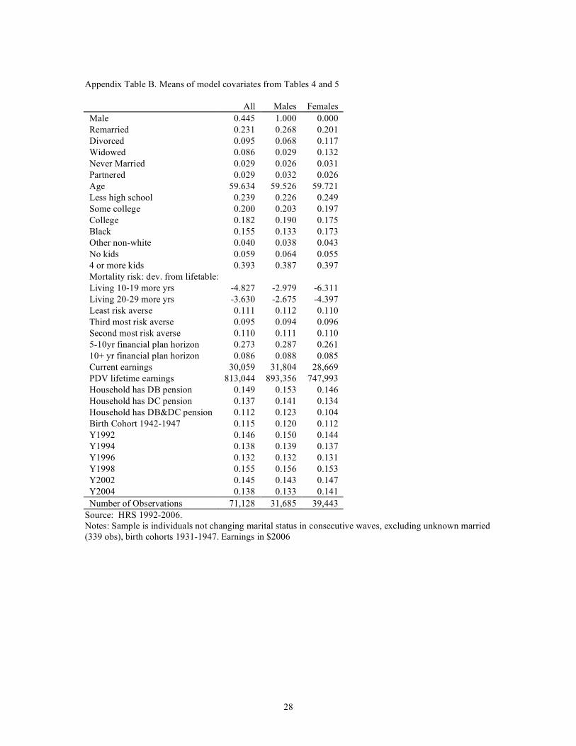
Appendix Table B. Means of model covariates from Tables 4 and 5 All Males Females Male 0.445 1.000 0.000 Remarried 0.231 0.268 0.201 Divorced 0.095 0.068 0.117 Widowed 0.086 0.029 0.132 Never Married 0.029 0.026 0.031 Partnered 0.029 0.032 0.026 Age 59.634 59.526 59.721 Less high school 0.239 0.226 0.249 Some college 0.200 0.203 0.197 College 0.182 0.190 0.175 Black 0.155 0.133 0.173 Other non-white 0.040 0.038 0.043 No kids 0.059 0.064 0.055 4 or more kids 0.393 0.387 0.397 Mortality risk: dev. from lifetable: Living 10-19 more yrs -4.827 -2.979 -6.311 Living 20-29 more yrs -3.630 -2.675 -4.397 Least risk averse 0.111 0.112 0.110 Third most risk averse 0.095 0.094 0.096 Second most risk averse 0.110 0.111 0.110 5-10yr financial plan horizon 0.273 0.287 0.261 10+ yr financial plan horizon 0.086 0.088 0.085 Current earnings 30,059 31,804 28,669 PDV lifetime earnings 813,044 893,356 747,993 Household has DB pension 0.149 0.153 0.146 Household has DC pension 0.137 0.141 0.134 Household has DB&DC pension 0.112 0.123 0.104 Birth Cohort 1942-1947 0.115 0.120 0.112 Y1992 0.146 0.150 0.144 Y1994 0.138 0.139 0.137 Y1996 0.132 0.132 0.131 Y1998 0.155 0.156 0.153 Y2002 0.145 0.143 0.147 Y2004 0.138 0.133 0.141 Number of Observations 71,128 31,685 39,443

Source: HRS 1992-2006. Notes: Sample is individuals not changing marital status in consecutive waves, excluding unknown married (339 obs), birth cohorts 1931-1947. Earnings in $2006