wake fields and impedance calculations of lhc collimators ... · wake fields and impedance...
TRANSCRIPT

Wake fields and impedance calculations ofLHC collimators’ real structures
Dipartimento di FisicaDottorato di Ricerca in Fisica degli Acceleratori – XXVIII Ciclo
CandidateOscar FrascielloID number 1224545
Thesis AdvisorsProf. Mauro MiglioratiDr. Mikhail Zobov
Co-AdvisorDr. Simone Di Mitri
A thesis submitted in partial fulfillment of the requirementsfor the degree of Doctor of Philosophy in Accelerator PhysicsOctober 2015

Wake fields and impedance calculations of LHC collimators’ real structuresPh.D. thesis. Sapienza – University of Rome
© 2015 Oscar Frasciello. All rights reserved
This thesis has been typeset by LATEX and the Sapthesis class.
Author’s email: [email protected]

To Lucia and Federico, for their conscious and unconscious patience...

iii
Acknowledgments
When I started working on the subject of wake fields and impedances in particleaccelerators, I did not know anything about how something that I always ascribedonly to the Ohm’s law could be of such a concern in particle’s world. Nor thatsomething I always thought to be fully revealed and described with superb clarity byJ. K. Maxwell, almost two centuries ago, could be of such an impressive and latestdevelopments.
Not even I ever thought to have the great chance and honour to work for twoprestigious and world renowned scientific institutions, the Italian National Institutefor Nuclear Physics, National Laboratories of Frascati (INFN-LNF) and the EuropeanCenter for Nuclear Physics (CERN), in Geneva. Despite the gratification, however,it was an hard challenge.
I owe to all those people who I encountered along the way, for their support andtheir contribution to my present experience.
Thanks to Mikhail Zobov, who has followed me as the principal supervisor ofthis PhD work, throughout the open up mysteries of wake fields and the stimulatingrequirements of the HiLumi LHC project. To Mauro Migliorati and Simone Di Mitri,for their careful support and the useful discussions. Thanks also to David Alesiniand Sandro Tomassini for their help, as well as to Alessandro Gallo, who let meresonate guitar strings apart from electromagnetic fields. Thanks to Andrea Ghigo,as the head of the LNF Accelerator Division, for having given me the opportunity tostart working in the field of Accelerator Physics and, thus, instilled the beginning ofthis work.
I am thankful to the CERN collegues Elias Metral, Benoit Salvant, NicolasMounet, Alexej Grudiev, Nicolò Biancacci and Luca Gentini. Thanks for the manyinformations shared, for the many discussions, for the support and for having listenedto me during the many meetings at CERN and around the world.
I devote special thanks to Warner Bruns, for his invaluable support, every time astuck, a bug or an “oops!” revealed their harmful potential.
Kind thoughts of gratitude are addressed to Adolfo Esposito, Maurizio Pelliccioniand Fiorello Martire, for their authentic friendship and the chance they gave me tolook forward into the future, once again, with passion. Among neutrons, photonsand all other charged particles, there is also the need to protect ourselves from fastmeals and lonely cigarettes. Thanks to Tiziano Ferro, for his presence and straightfriendship.
To you, being always with me even if we never find a way to meet, so far but sobrotherly close to each other, what loving does really mean...grazie Compare!
Thanks to my large family, no words are needed to explain why.Thanks to life, for having opened up the real beauty to my eyes and inspired the
dedication of this work, day by day.This work was supported by HiLumi LHC Design Study, which is included in
the High Luminosity LHC project and is partly funded by the European Commissionwithin the Framework Programme 7 Capacities Specific Programme, Grant Agreement284404.

iv
Eppur ti vidi nascere,al chiarore di un sole sbiaditoin un timido autunno.Remissivi si fecer da parte,lasciando il cielo obnubilatoe anelo del suo albore,al fulgor dei giorni nostri.Di tal bellezza ci commovemmo,di magnifica pienezzatuoi devotici iniziasti a vivere.
Oscar Frasciello

v
Abstract
The Large Hadron Collider (LHC) hosted at CERN, the European Organization forNuclear Research in Geneva, Switzerland, is the world’s largest particle accelerator.With a circumference of 27 km, it can bring proton beams into collitions at a centreof mass energy of 14 TeV. It has been conceived and built to let scientific researchto explore the high energy physics frontiers, keeping collision events at a designluminiosity of 1034 cm≠2s≠1.
Beyond this goal challenging in itself, the High Luminosity LHC (HiLumi-LHC)project aims at increasing the LHC luminosity by an order of magnitude and one ofthe key ingredients to achieve that is to increase beam intensity. In order to keepbeam instabilities under control and to avoid excessive power losses a careful designof new vacuum chamber components and continuous update and improvement ofthe LHC impedance model are required.
Collimators are among the major impedance contributors. During LHC Run I,measurements with beam have revealed that the betatron coherent tune shifts werehigher by about a factor of 2 with respect to the theoretical predictions based onthe impedance model up to 2012. In that model the resistive wall impedance wasconsidered as the dominating impedance contribution for collimators. By means ofGdfidL electromagnetic code simulations, the geometric impedance of secondary andtertiary (TCS/TCT) collimators’ real structures (i.e. not simplified) was calculated,contributing to the update of the LHC impedance model. This resulted also in abetter agreement between the measured and simulated betatron tune shifts.
During the LHC Long Shutdown I (LS I), some of the Run I TCS and TCTcollimators were replaced by new devices, embedding Beam Position Monitor (BPM)pick-up buttons in the tapering regions, in order to provide accurate and continuousmeasurements of the beam centres, and ferrite blocks for the damping of the HigherOrder Modes (HOMs) trapped in the collimators’ structure.
The injection collimators (TDI) are undergoing a substantial design review andupgrade study stage, as part of the whole LHC injection protection system upgradeforeseen to be finished in the LHC LS II (2018-2019). Measurements performed duringLHC Run I have shown that the presently installed TDIs contribute significantlyto both longitudinal and transverse impedance, determining beam induced heatingand high vacuum pressure that a�ected background of experiments. In the view ofhigher intensities planned for the Run III and HiLumi-LHC operations, all theseimpedance related issues have to be minimized.
The aim of this work was to perform accurate simulations of collimators’impedance, which has become very important and challenging. Accurate doesmean as close as possible to the real conditions. Thus, in order to a�ord such a task,the huge collimators’ CAD designs were used as input into GdfidL code. Besides,several dedicated tests have been performed to verify correct simulations of lossydispersive material properties, such as resistive wall and ferrites, benchmarking coderesults with analytical, semi-analytical and other numerical codes outcomes. Theresults of the collimators wake fields and impedances calculations, together withtheir comparison with experimental measurements are shown and discussed.

vi
Contents
1 Introduction 31.1 The CERN Large Hadron Collider . . . . . . . . . . . . . . . . . . . 31.2 The High Luminosity LHC project . . . . . . . . . . . . . . . . . . . 71.3 The LHC collimation system . . . . . . . . . . . . . . . . . . . . . . 9
2 Wake fields and beam coupling impedances 142.1 Where do Wake fields originate from . . . . . . . . . . . . . . . . . . 142.2 Panofsky-Wenzel theorem and Wake functions . . . . . . . . . . . . . 19
2.2.1 Basic approximations . . . . . . . . . . . . . . . . . . . . . . 192.2.2 The Panofsky-Wenzel theorem . . . . . . . . . . . . . . . . . 202.2.3 Decomposition into modes and Wake functions definition . . 212.2.4 General properties of Wake functions . . . . . . . . . . . . . . 23
2.3 Wake Potentials . . . . . . . . . . . . . . . . . . . . . . . . . . . . . . 242.4 Beam coupling Impedance . . . . . . . . . . . . . . . . . . . . . . . . 25
2.4.1 Longitudinal impedance . . . . . . . . . . . . . . . . . . . . . 252.4.2 Transverse impedance . . . . . . . . . . . . . . . . . . . . . . 272.4.3 General properties of impedances . . . . . . . . . . . . . . . . 272.4.4 Resonator impedance . . . . . . . . . . . . . . . . . . . . . . 292.4.5 Bunch modes . . . . . . . . . . . . . . . . . . . . . . . . . . . 312.4.6 Loss factor, kick factor and e�ective impedance . . . . . . . . 35
2.5 Collective e�ects . . . . . . . . . . . . . . . . . . . . . . . . . . . . . 382.5.1 Single bunch . . . . . . . . . . . . . . . . . . . . . . . . . . . 382.5.2 Multi-bunch . . . . . . . . . . . . . . . . . . . . . . . . . . . . 40
3 LHC Run I TCS-TCT collimators 423.1 Theoretical considerations . . . . . . . . . . . . . . . . . . . . . . . . 45
3.1.1 Geometric and resistive wall kick factors evaluation . . . . . . 463.2 Numerical calculations . . . . . . . . . . . . . . . . . . . . . . . . . . 473.3 LHC impedance model update . . . . . . . . . . . . . . . . . . . . . 50
4 Simulation tests of resistive and dispersive properties of materialsin GdfidL 564.1 RW simulation tests . . . . . . . . . . . . . . . . . . . . . . . . . . . 56
4.1.1 Resistive cylindrical pipe . . . . . . . . . . . . . . . . . . . . 564.1.2 Beam pipe with thick resistive insert . . . . . . . . . . . . . . 59
4.2 Ferrite Material Simulation Test . . . . . . . . . . . . . . . . . . . . 61

Contents vii
4.2.1 Scattering parameter S11
of a coaxial probe . . . . . . . . . . 634.2.2 Impedance of a ferrite filled pillbox . . . . . . . . . . . . . . . 654.2.3 Tsutsui model for TT2-111R ferrite kicker . . . . . . . . . . . 66
5 LHC Run II TCS/TCT collimators 735.1 New TCS/TCT’s taper design optimization study . . . . . . . . . . 74
5.1.1 Resistive wall impedance contribution from the new angle set 765.2 TCS/TCT impedance study . . . . . . . . . . . . . . . . . . . . . . . 78
5.2.1 S1x
parameters simulations vs loop measurements . . . . . . 815.2.2 Z‹ simulations versus wire measurements . . . . . . . . . . . 82
6 LHC TDI collimators 886.1 TDI taper optimization study . . . . . . . . . . . . . . . . . . . . . . 896.2 TDIS’ real structures impedance study . . . . . . . . . . . . . . . . . 91
7 Conclusions 98
A The linear accelerator model 100
B The GdfidL Finite Di�erence code 102

1
PhD activity related outcomes
Publications1. N. Biancacci et al., “Impedance simulations and measurements on the LHC
TCTP collimators with embedded BPMs”, Physical Review Special Topics -Accelerators and Beams, to be submitted.
2. O. Frasciello et al., “Geometric beam coupling impedance of LHC secondarycollimators”, Nuclear Instruments and Methods in Physics Research SectionA, 2015. DOI:10.1016/j.nima.2015.11.139
3. O. Frasciello et al., “Numerical Calculations of Wake Fields and Impedancesof LHC Collimators’ Real Structures”, Proceedings of ICAP 2015, Shanghai,China. arXiv:1511.01236.
4. J. Uythoven et al., “Injection protection upgrade for the HL-LHC” , Proceedingsof IPAC 2015, Richmond, VA, USA, TUPTY051.
5. B. Salvant et al., “Expected Impact of Hardware Changes on Impedanceand Beam-induced Heating during Run 2”, Proceedings of LHC PerformanceWorkshop, Chamonix, France, September 22-25, 2014.
6. The HiLumi LHC Collaboration, “HL-LHC Preliminary Design Report : De-liverable: D1.5”, CERN-ACC-2014-0300.
7. E. Metral, “Beam intensity limitations”, CERN-ACC-2014-0297.
8. O. Frasciello et al., “Geometric beam coupling impedance of LHC secondarycollimators”, Proceedings of IPAC 2014, Dresden, Germany, TUPRI049.
9. N. Mounet et al., “Tranverse impedance in the HL-LHC era”, CERN-ACC-SLIDES-2014-0085.
Scientific talks1. “Numerical Calculations of Wake Fields and Impedances of LHC Collimators’
Real Structures”, Invited talk at ICAP 2015, October 16th, 2015, Shanghai,China.

Contents 2
2. “Wake fields and impedances of LHC collimators”, Invited talk at 100thNational Congress of the Italian Physical Society (SIF), September 22 - 262014, Pisa, Italy.
3. “Beam coupling impedance of the new LHC collimators”, Contributed talk at101st National Congress of the Italian Physical Society (SIF), September 24th2015, Rome, Italy.
4. “Present status and future plans of LHC collimators wake fields and impedancessimulations”, Contributed talk at BE-ABP Impedance meeting, March 23rd2015, CERN, Geneva, Switzerland.
5. “Wake fields and impedances calculations with GdfidL, MMM and CST forbenchmarking purposes”, Contributed talk at BE-ABP Impedance meeting,February 2nd 2015, CERN, Geneva, Switzerland.
6. “Wake fields and impedances simulations of LHC collimators with GdfidLcode”, Contributed talk at 4th HiLumiLHC-LARP Annual Meeting, November19th 2014, KEK, Tsukuba, Japan.
7. “Wake fields and impedances simulations of LHC collimators with GdfidLcode”, Contributed talk at 17th meeting HiLumi-LHC WP 2.4, October 29th2014, CERN, Geneva, Switzerland.
8. “Test simulations of TT2-111R lossy dispersive material properties”, Con-tributed talk at 8th meeting HiLumi-LHC WP 2.4, March 26th 2014, CERN,Geneva, Switzerland.
9. “Geometric coupling impedance of LHC secondary collimators”, Contributedtalk at Topical Workshop on Instabilities, Impedance and Collective E�ects2014 (TWIICE2014), January 16-17 2014, SOLEIL, France.
Posters1. O. Frasciello et al., “Geometric beam coupling impedance of LHC secondary
collimators”, IPAC 2014, Dresden, Germany.
2. O. Frasciello et al., “Beam coupling impedance of LHC secondary collimators”,X international scientific workshop to the memory of professor V.P. Sarantsev,Alushta, Ukraine.

3
Chapter 1
Introduction
1.1 The CERN Large Hadron ColliderThe Large Hadron Collider (LHC) hosted at CERN, the European Organization forNuclear Research in Geneva, Switzerland, is the world’s largest particle accelerator.With a circumference of 27 km, it can bring into collisions proton beams at acentre of mass energy of 14 TeV. It is the last element of a more complex chain ofaccelerators (Fig. 4.4). Each machine of this chain injects the beam into the next
Figure 1.1. A sketch of the whole LHC accelerator complex, together with the mainexperiments and beam lines.
one at increasing energy. First, Hydrogen atoms are ionized by a DuoplasmatronProton Source, stripping orbiting electrons and producing protons to be injectedinto Linac 2. Linac 2 accelerates protons up to the energy of 50 MeV, before theyare transferred to the Proton Synchrotron Booster (PSB) which brings them to 1.4GeV. Protons are again transferred in sequence to the Proton Synchrotron (PS) and

1.1 The CERN Large Hadron Collider 4
the Super Proton Synchrotron (SPS) where they reach energies of, respectively, 25GeV and 450 GeV. At the end of the SPS stage, protons are ready to feed the LHCwhere they are accelerated to the final energy of 7 TeV. The SPS injects two bunchedbeams into the LHC, B1 and B2, via two transfer lines, TI2 and TI8, according tothe filling schemes in Fig. 4.5[1].
Figure 1.2. Bunches in the LHC, SPS and PS. PS batch consists of 72 bunches on h = 84at extraction. Either three or four of these batches are sequentially transferred to theSPS, thereby partially filling 3/11 or 4/11 of the SPS circumference. For each LHC ring,12 of these 216 or 288 bunch trains are transferred from SPS to LHC. With 9 ·216+3 ·288injections, the LHC is filled with 2808 bunches.
The accelerator complex can accelerate not only protons, but also Lead ions,produced heating to a temperature of about 500°C a highly purified lead sample,then ionizing the formed vapours by means of an electron current. The Pb29+ ionsare accelerated to 4.2 MeV/u and brought to impinge on carbon foils to be strippedto Pb54+. These latter ions constitutes the intermediate beam accumulated in theLow Energy Ion Ring (LEIR) and accelerated to 72 MeV/u before being injected intothe PS, which lets the beam to reach the energy of 5.9 GeV/u. This is the energy atwhich the SPS is fed by the ion beam, finally stripped to Pb82+ and accelerated to177 GeV/u before being finally transferred to the LHC, where Pb82+ ion beams willbe accelerated at 2.76 TeV/u.
The nominal energy stored per beam in the LHC is about 362 MJ, what char-acterize the LHC as a record machine both from the stored energy and the energydensity points of view (Fig. 1.3(a) and Fig. 1.3(b)) [2]. Such an extreme facility putsstrong contraints on the reliability of the safety and the collimation systems. Theformer has the role of aborting the beams in a clean way in case of any dangerouscondition; the latter one has to protect the machine and detectors from halo particlesand other unavoidable losses, as will be further discussed in more detail in section1.3.

1.1 The CERN Large Hadron Collider 5
(a)
(b)
Figure 1.3
A schematic layout of LHC is shown in Fig. 1.4. There are eight arcs housing154 dipole bending magnets and eight straight sections housing LHC detectors infour of them and other machine utilities, such as radiofrequency, collimators andbeam dumps in four others. The four detectors are:
• ALICE (A Large Ion Collider Experiment), which studies the properties ofquark-gluon plasma;
• ATLAS (A Toroidal LHC ApparatuS), designed to study a wide range ofPhysics at LHC, from the search for Higgs Boson[3, 4] to supersymmetries(SUSY) and extra dimensions;
• CMS (Compact Muon Solenoid), aimed at the same Physics hunt as ATLASbut with di�erent technical solutions;

1.1 The CERN Large Hadron Collider 6
• LHCb (LHC Beauty), designed to study asymmetries between matter andantimatter in B particles interactions.
Figure 1.4
All the above mentioned detectors study very rare events. The number of eventsper second generated by beam-beam collisions for a given process is given by
N = L‡, (1.1)
where L is the luminosity and ‡ the cross section for the process under study. Theluminosity is a crucial figure of merit for a particle collider and for rare events thedemand is for it to be as large as possible, 1034cm≠2s≠1 for LHC. Depending only onthe beam parameters, the luminosity for a Gaussian beam profile can be written as
L = N2
b
nfr
“
4fi‘n
—ú , (1.2)
where Nb
is the number of particles per bunch, n the number of bunches per beam,f
r
the revolution frequency, “ the relativistic Lorentz factor, ‘n
the normalizedtransverse emittance and —ú the — function at collision points. The integratedluminosity performances over three years of operation, reported in Table 1.1, togetherwith the machine operational parameters before LS I reported in Table 1.2[5], allowedATLAS and CMS to discover the Higgs Boson1 [7, 8, 9, 10].
1ATLAS and CMS collaborations announced the Higgs boson discovery on July 4th, 2012 duringa joint seminar at CERN. More recently, the LHCb experiment claimed for pentaquark discoveryon July 14th, 2015[6].

1.2 The High Luminosity LHC project 7
Year Overview COM Integrated Luminosity [fb≠1]2010 Commissioning 7 TeV 0.042011 Exploring limits 7 TeV 6.12012 Performance 8 TeV 23.1
Table 1.1. LHC operations 2010-2012
Parameter Value in 2012 Design valueBeam energy [TeV] 4 7—ú in IP 1,2,5,8 [m] 0.6,3.0,0.6,3.0 0.55Bunch spacing [ns] 50 25Number of bunches 1374 2808
Average bunch intensity [p/bunch] 1.6-1.7·1011 1.5·1011
Normalized emittance at start of fill [mm mrad] 2.5 3.75Peak luminosity [cm≠2s≠1] 7.7·1033 1·1034
Max. mean number of events per bunch crossing ¥ 40 19Stored beam energy [MJ] ¥ 140 362
Table 1.2. Performance related parameter overview
1.2 The High Luminosity LHC projectThe European strategy for particle physics has, as its highest priority, the fullexploitation of the LHC discovery capabilities [11, 12]. In order to extend LHCpotential, a substantial upgrade is needed to increase the luminosity beyond itsdesign values, by a factor of 5 the instantaneous luminosity and by a factor of 10 itsintegrated one. According to the baseline programme until 2025 shown in Fig. 1.5,this upgrade is planned to take place in 2020s [13].
Figure 1.5. LHC baseline plan for the next decade. The red upper line shows collisionenergy while the green lower lines the integrated luminosity.
Several innovative technologies will support the reliability of the novel machine,High Luminosity LHC (HL-LHC hereinafter), such as 11-12 tesla Super Conducting(SC) magnets, ultra compact SC cavities for ultra precise phase control and beam
1.2 The High Luminosity LHC project 8
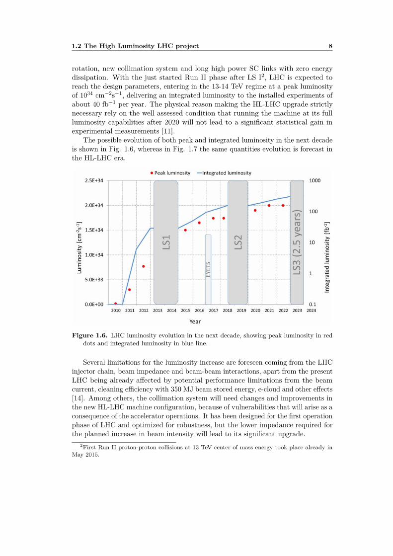
rotation, new collimation system and long high power SC links with zero energydissipation. With the just started Run II phase after LS I2, LHC is expected toreach the design parameters, entering in the 13-14 TeV regime at a peak luminosityof 1034 cm≠2s≠1, delivering an integrated luminosity to the installed experiments ofabout 40 fb≠1 per year. The physical reason making the HL-LHC upgrade strictlynecessary rely on the well assessed condition that running the machine at its fullluminosity capabilities after 2020 will not lead to a significant statistical gain inexperimental measurements [11].
The possible evolution of both peak and integrated luminosity in the next decadeis shown in Fig. 1.6, whereas in Fig. 1.7 the same quantities evolution is forecast inthe HL-LHC era.
Figure 1.6. LHC luminosity evolution in the next decade, showing peak luminosity in reddots and integrated luminosity in blue line.
Several limitations for the luminosity increase are foreseen coming from the LHCinjector chain, beam impedance and beam-beam interactions, apart from the presentLHC being already a�ected by potential performance limitations from the beamcurrent, cleaning e�ciency with 350 MJ beam stored energy, e-cloud and other e�ects[14]. Among others, the collimation system will need changes and improvements inthe new HL-LHC machine configuration, because of vulnerabilities that will arise as aconsequence of the accelerator operations. It has been designed for the first operationphase of LHC and optimized for robustness, but the lower impedance required forthe planned increase in beam intensity will lead to its significant upgrade.
2First Run II proton-proton collisions at 13 TeV center of mass energy took place already inMay 2015.

1.3 The LHC collimation system 9
Figure 1.7. HL-LHC luminosity evolution, showing peak luminosity in red dots andintegrated luminosity in blue line.
1.3 The LHC collimation systemBunched3 particle beams are generally characterized by a Gaussian-like distributionof particles in the transverse plane. So within one standard deviation, 1 ‡, of theGaussian beam ≥68% of the particles are comprised. Looking at Fig. 1.8, the beamcore is usually defined as 0 ≠ 3 ‡ (99.7% of all particles), while the region > 3 ‡is recognized as the beam halo. For the LHC the beam profile is more parabolic-like then Gaussian-like. However no lack of validity is found in what follows, if aGaussian-like distribution is assumed.
Partial or total beam losses are unavoidable in particle accelerators. Thereare several e�ects leading to beam losses, such as collisions in interactions points,interactions with residual gas in vacuum systems and intra-beam scattering, beaminstabilities (single bunch, multi-bunch, beam-beam e�ects), dynamic changes drivenby machine operational cycle (orbit drifts, optics changes), RF noises and out-of-bucket losses, injection and dump losses. All these e�ects can increase the beam halopopulation and ultimately cause beam losses. Their mechanisms are charachterizedby a time-dependent beam lifetime during the machine cycle, ·
b
, where the beamintensity time dependence is given by
I(t) = I0
· e≠ t
·
b , (1.3)
and the particle loss rate by≠ 1
I0
dI
dt= 1
·b
. (1.4)
As an example, with ·b
= 1 h and I0
= 3.2 ·1014 p, the total loss per second would be90 · 109 p/s, or 0.1 MJ/s= 100 kW. Again, at 7 TeV only 1% of total beam intensity
3Bunched beams are formed by “packets” or pulses of particles named bunches. On the contrary“coasted” or unbunched beams have no longitudinal substructure.

1.3 The LHC collimation system 10
Figure 1.8. Core and halo definition for a particle beam with Gaussian transverse particledistribution.
loss in a period of 10 s, would produce a peak load of 500 kW, whereas the upperlimit to SC magnets energy deposition, without quench, is ≥8.5 W/m.
Collimation system has been designed to accomplish several tasks, such as SCmagnets protection agains quenching, beam halo cleaning throughout the LHC beamcycle (reaching an e�ciency of 99.998%), its diagnostic and scraping, machine aper-ture passive protection against radiation and hardware protection against radiationhardness [15, 16, 17]. For the collimation system to be successful in all the assignedtasks means to be subtended to the condition that all losses occur at collimators, andnot elsewhere in the machine. This entails all particles’ oscillations growing to largeamplitudes having to be intercepted by the collimators, thus protecting the machine.Collimators are placed around the beam with various settings of longitudinal positionorientation in the H-V transverse planes and transverse distances from the beam.Fig. 1.9 shows the collimators’ layout in the LHC machine, with the three stage
collimation system installed in the dedicated cleaning insertions IP3 and IP7, toensure that only a small fraction of lost protons escapes from there, while in Fig.1.10 the LHC collimation hierarchy is depicted, with collimators disposition withrespect to the beam core depending upon material robustness. Generally low Zmaterials, like Carbon Fiber Composite (CFC), ensure for higher robustness at theexpenses of absorption power.
The collimators’ design relies on two parallel jaws that define a slit for the beampassage(Fig. 1.11(a)) [19]. The collimator whole box (Fig. 1.11(b)) can be rotated

1.3 The LHC collimation system 11
Figure 1.9. The LHC collimations system layout. Two three-stages cleaning insertions arinstalled in IP3 and IP7. Other absorber collimators are distributes along the machine.Injection collimators are also shown near IP2 and IP8.
in the H-V plane to collimate horizontal, vertical or skew halo, as shown in Fig.1.12(a),1.12(b) and 1.12(c).
The collimation hierarchy is composed of:
• Primary collimators (TCP) with Carbon Fiber Composite (CFC) jaws;
• Secondary collimators (TCS) made again of CFC jaws;
• Tertiary collimators absorbers with Tungsten (W) or Copper (Cu) made jaws.
Among others, injection collimators (TDI) are noteworthy also, with important rolein beam cleaning at the exit of SPS and local protection against injection failures.Table 1.3 summarizes some TCP and TCS collimators specifications, while in Table1.4 the main specifications for other LHC ring collimators are listed.
TCP collimators intercept stray particles of the primary halo for horizontal,vertical, skew or momentum o�sets, spraying losses downstream. Further losses ofsecondary halo particles interception and dilutions happen at TCS collimators. Atthe end of the warm cleaning insertions, less robust high Z (W, Cu) jaws collimatorsabsorb the diluted proton halo and showers. After this three-stage cleaning process,

1.3 The LHC collimation system 12
Figure 1.10. LHC collimation hierarchy. Collimators are disposed in order to protect themachine against primary, secondary and tertiary radiation fields and hadronic showersproduced by the interaction of the primary proton beam halo [18].
(a) (b)
Figure 1.11. Photograph of a TCP/TCS LHC Run I type collimator along the beam path(a) and of a TCP/TCS LHC Run I type collimator box during assembling (b).
finally, a fourth stage takes place again with high Z jaws collimators, having tointercept tertiary halo close to the particle physics experiments and triplet magnets.
The LHC collimation design has taken into account many requirements, onebeing the coupling impedance whose transverse and longitudinal component dependsstrongly on collimator settings, both at injection and at top energy, given thecollimation gaps going down to 2.5 mm and a total installed collimators’ jaw lengthof about 48 m per beam [20, 21]. The LHC performance relies upon beam cleaninge�ciency and coupling impedance, both potentially constituting a limitation in themaximum achievable beam intensity.

1.3 The LHC collimation system 13
(a) (b) (c)
Figure 1.12. Collimators orientation in horizontal (a), vertical (b) and skew (c) planes,with the beam sketched as a red spot.
Parameter TCP TCSJaw material CFC CFC
Jaw length [cm] 60 100Jaw tapering [cm] 10 + 10 10 + 10
Jaw cross section [mm2] 65 · 25 65 · 25Jaw resistivity [µ�m] Æ 10 Æ 10
Heat load [kW] Æ 7 Æ 7Jaw temperature [°C] Æ 50 Æ 50
Residual vacuum pressure [mbar] Æ 4 · 10≠8 Æ 4 · 10≠8
Minimal gap [mm] Æ 0.5 Æ 0.5Maximal gap [mm] Ø 58 Ø 58
Maximumm Jaw angle [mrad] 2 2Table 1.3. Some specifications for TCP and TCS collimators.
Parameter TCT TCLA TCL TCLP TCLIJaw material W W Cu Cu CFC
Jaw length [cm] 100 100 100 100 100Jaw tapering [cm] 10+10 10+10 10+10 10+10 10+10Minimal gap [mm] Æ 0.8 Æ 0.8 Æ 0.8 Æ 0.8 Æ 0.5
Table 1.4. Some specifications for other LHC ring collimators.
In the next chapter the concepts of wake fields and beam coupling impedances willbe expolited. Their influence on particle beam dynamics by means of induced beaminstabilities will be addressed also. Comprehensive and fully exhaustive treatmentsof collective beam instabilities exist elsewhere and are referred to [22, 23] throughoutthis thesis but are not its main subject, so that the discussion will be focused onlyon those type of instabilities of concern for the study conducted on LHC collimators.

14
Chapter 2
Wake fields and beam couplingimpedances
2.1 Where do Wake fields originate fromThe motion of charged particles in the electromagnetic fields (E, B) is governed bythe Lorentz force F [24]:
m0
“dv
dtF = q(E + v ◊ B), (2.1)
“ being the Lorentz energy factor “ = 1/
1 ≠ —2, — = v/c. The design of anaccelerator relies on the consideration of the motion of a single charged particle inthe environment of magnets and RF cavities, which must be stable (i.e. the particleand the beam lifetime must be long enough to allow su�cient luminosity to theinstalled physics experiments). So that, in what is usually called the linear latticedesign for a circular machine, three basic elements are addressed:
• the Dipoles which guides the particle trajectory via the magnetic field, weaklyfocusing in the transverse horizontal x direction;
• the Quadrupoles which confines the particle motion near the design trajectoryvia the magnetic field, focusing in the transverse x and y directions;
• the Sextupoles and higher order multipole magnets for the control of chromaticand geometric aberrations;
• the RF cavities which keep the particle energy near the design energy via theelectric field, thus focusing in the longitudinal z direction.
A charged particle moving on a circular orbit is sketched in Fig. 2.1, in which thethree directions x, y and z above referred to are specified.
There are, however, additional electromagnetic fields coming from the interac-tion of the charged beam particle (here called source) with its vacuum chamberenvironment in the accelerator. The interaction takes place owing to the Gauss’slaw, which for a charge in free space reads
Ò · E = fl
‘0
, (2.2)

2.1 Where do Wake fields originate from 15
R
Ox
y
z
s = vt
Figure 2.1. A simple sketch of a reference charged particle moving on a circular orbit,specifying the reference coordinate system.
where fl is the charge density at the point where the field is E and ‘0
is the electricpermittivity of free space, equal to 8.854 ◊ 10≠12 F/m, in the SI system of units. Itsphysical meaning is that electric field lines are absolutely attached to the charges,they can be distorted but never cut away from the charges under any circumstances.If the charge is in free space and stationary, its electric field lines radiate outwardsisotropically, as in Fig. 2.2(a). As a result of the theory of relativity, if the chargemoves relativistically with velocity v ¥ c, c = 2.997925 ◊ 108 m/s being the velocityof light, electric field lines get contracted into a thin disk, usually called “pancake”,perpendicular to the particle’s direction of motion with an angular spread of 1
“
, asin Fig. 2.2(b). When the charge moves in the ultrarelativistic limit v = c, then thepancake reduces to ”-function thin sheet, as shown in Fig. 2.2(c)[22].
q
~E
v = 0
(a)
q
~E
v ⇡ c
(b)
q
~E
v = c
(c)
Figure 2.2. Electric field lines for a charge in free space a) stationary, b) moving relativis-tically and c) in the ultrarelativistic limit.
Magnetic field is also generated by a moving charge, with the same distribution asthe electric field but with di�erent properties. It also get contracted into a pancake-like thin disk as v approaches c, but its direction is azimuthal instead of radial asthe electric field direction. Choosing a cylindrical coordinate system to describe theparticle motion in free space, (r, ◊, s), in which s is the absolute longitudinal positionin the laboratory frame, thus pointing in the direction of motion of the charge q,the application of the Gauss’s law 2.2 for the electric field and of the Ampere’s law

2.1 Where do Wake fields originate from 16
for the magnetic field
Ò ◊ B = µ0
j + 1c2
ˆE
ˆt, (2.3)
where µ0
is the magnetic permeability of vacuum equal to 4fi ◊ 10≠7 H/m in theSI system of units and j is the current density vector, the following relations forelectric and magnetic fields can be obtained for the moving charge considered:
Er
= 2q
r”(s ≠ ct) (2.4)
B◊
= 2q
r”(s ≠ ct). (2.5)
The situation in which a particle moves in the vacuum chamber of an acceleratordeserves a bit more of discussion. Let the particle move along the axis of an axiallysymmetric perfectly conducting vacuum chamber pipe, as shown in Fig. 2.3. Let
q c
�q
Perfectly conducting wall
(a)
Beam
Test charge
Image charges
� �
e v = c
v = c+ +
(b)
Figure 2.3. Particle a) and beam b) moving on axis in a perfectly conducting wall vacuumchamber. Image charges are shown on the wall.
the pipe be smooth1. The solution again of the Gauss’s and Ampere’s laws leadsto the same equations 2.2 and 2.3, but with the field lines perfectly terminatingon the pipe wall (Fig. 2.3(b)). The image charges on the wall is exactly equal andopposite to that of the particle (or the beam), moving with the same velocity v = cin the same direction. The entire field pattern moves with it and no field are leftbehind. Both in free space or in perfectly conducting pipe, the dependece of 2.4 on
1This means that it has no discontinuities.

2.1 Where do Wake fields originate from 17
”(s ≠ ct) makes the ultrarelativistic particle not to feel any e�ect from the fieldscarried by other particles in the beam. This is unless any two particles move side byside exactly at the same longitudinal position, in which case however electric andmagnetic fields cancel exactly thus producing no Lorentz force on the particles. Toillustrate the above statement, consider the “test charge” depicted in Fig. 2.3(b),which moves with the beam and has the same charge sign, v = c. This particle willexperience two forces, the electrical F
E
= e · E due to the electric field of the beam,directed radially, and the magnetic F
B
= e(v ◊ B)/c directed along the azimuthaldirection, by means of the right hand rule. F
E
will push the charge e towards thepipe wall whereas F
B
will point towards the pipe axis, but in the ultrarelativisticlimit
---E--- =
---B--- and the two forces cancel exactly. As a consequence, it can be stated
that if the beam is ultrarelativistic, the vacuum chamber is smooth and perfectlyconducting, no collective instabilities can occur.
When there is a discontinuity in the conducting vacuum chamber, the imagecharges moving along the pipe have now to move around a corner. It is a wellestabilished result of the electromagnetic theory that when a charge is bent itradiates. Thus additional electromagnetic fields are generated as the radiation fieldsof the image charges when their trajectory is bent. Because of causality, such fieldsexist behind the particle and thus are called wake fields. This physical mechanism isillustrated in Fig. 2.4 and Fig. 2.5.
(a) (b)
Figure 2.4. Charged beam passing through a) a smooth pipe and through b) a pipe withdiscontinous sturcure [22]. Only in the latter case wake fields are generated, as specifiedin Fig. 2.5.
An intense beam will generate a strong wakefield and the stronger the wakefieldthe more the beam can become unstable. Wakefields will perturb the motion of thefollowing particles, called witness. This way a particle can experience an “e�ective”electromagnetic field given by the sum of the one produced by the external latticeelements of the accelerator, and the other being the wakes produced by the particlesin front interacting with the vacuum chamber, so that [23]:
(E, B)effective
= (E, B)external
+ (E, B)wakes
.

2.1 Where do Wake fields originate from 18
(a) (b) (c)
Figure 2.5. Wake fields generated as the the beam passes along the axis of a discontinousvacuum chamber. In the smooth region in a) no wake fields generate; they start topropagate as soon as the beam approaches the discontinuity in b) and continue propagateinside the structure when the beam as passed away in c) [22].
The two fields summed on the right hand side (RHS) of the equation di�ers in(E, B)
external
being beam intensity indipendent, while (E, B)wakes
being proportionalto beam intensity. The wakes’ influence on the beam can be trated as a perturbationif the condition (E, B)
wakes
π (E, B)external
is satisfied. The wake fields generatedin the case of perfectly conducting vacuum chamber walls, due to its geometricaldiscontinuities only, are referred to as “geometric wake fields” [25].
If the vacuum chamber wall is still smooth but has finite constant electricconductivity ‡ (i.e. it is resistive), the so called “resistive wall” (RW) wake fields aregenerated. To understand the physical mechanism a brief recall of the main results ofMaxwell equations is needed, as illustrated in Fig. 2.6. Electric and magnetic fields
Equation of continuity
Maxwell equations
⇢, � ~J, ~K
~E ~B
driving driving
Figure 2.6. A logical sketch of the physical content of Maxwell equations. By definition,metals have fl = 0 and J = ‡E, whereas insulators have J = 0 and fl = ‘Ò · E.
are driven by, respectively, charges and currents. The interplay between electric andmagnetic fields is governed by Maxwell equations, while that of charge and currentby the equation of continuity. In the case of metals, charges stay on the surface andare not allowed inside, while currents stay near the surface and do penetrate intothe conductor. The parameter quantifying how much they do penetrate is the skindepth
”skin
= c
2fi‡|Ê|, (2.6)

2.2 Panofsky-Wenzel theorem and Wake functions 19
where ‡ is the finite conductivity of the metal and Ê the frequency of the electromag-netic field. For insulators, instead, no currents but charges are allowed to stay inside.Thus the physical mechanism giving rise to RW wake fields lies on electric fieldlines being terminated by a surface charge on the wall surface and on the magneticfield being cancelled by a surface current, when the beam’s image charges flow onthe vacuum chamber wall. While electric field is terminated by surface currents,magnetic field is “mostly” cancelled, because currents have penetrated the wall by askin depth. The image currents can re-surface from the chamber wall after the pointcharge has past and drive new magnetic fields that in turn drive new electric fieldsby Maxwell equations. In the case of RW wake fields, they are mainly magnetic fieldscontributing to transverse wake force, while the associated electric field contributesto longitudinal wake force.
The qualitative discussion on the origin of wake fields will be exploited in mathe-matical detail in the next section, where the concept of beam coupling impedance willarise. This will allow to gain useful informations on the beam dynamics in presenceof wake fields and to analyze the beam dynamics subtended to those collectiveinstabilities the work described in the next chapters will concern with.
2.2 Panofsky-Wenzel theorem and Wake functions2.2.1 Basic approximationsTwo basic approximations are introduced in order to simplify the mathematicaldescription of wake functions, the rigid bunch and the impulse approximations [22].
In the rigid bunch approximation, the beam traversing through the vaccumchamber is assumed to be not a�ected by its discontinuities. Looking at Fig. 2.7,s is the distance of the source particle along the vacuum chamber axis, from anarbitrary reference point. Let the source particle be at s = —ct and the following(here called witness) particle at s = z + —ct, with z < 0 to indicate that the witnessstays behind the source. Being the bunch rigid, both z and —c do not change aftertraversing the discontinuity, even if synchrotron motion is still allowed.
z
~v switness
source
Figure 2.7. The rigid bunch approximation. Both distance between source and witness par-ticles, z, and particles velocity, —c, do not change during vacuum chamber discontinuitiestraversal.
Let q be the witness particle charge. The impulse approximation relies on nothingof the single E or B components of the wake field or wake force F in theirselves

2.2 Panofsky-Wenzel theorem and Wake functions 20
being considered, but only the change in impulse of the witness particle
�p =Œ⁄
≠Œ
F dt =Œ⁄
≠Œ
q(E + v ◊ B) dt. (2.7)
2.2.2 The Panofsky-Wenzel theoremLet the Maxwell equations be rewritten for the witness particle at (x, y, s, t), with zconstant and s = z + —ct,
Ò · E = fl
‘0
(2.8)
Ò ◊ B = µ0
—cfls (2.9)Ò · B = 0 (2.10)
Ò ◊ E = ≠ˆB
ˆt, (2.11)
where s is the unit vector of the s direction.Given the Lorentz force definition in eq. 2.1, the Panofsky-Wenzel theorem arise
quite naturally from eqs. 2.8- 2.11 written for the change in impulse �p(x, y, z, t).For instance, the calculation of the divergence and curl of Lorentz force leads to:
Ò · F = q(Ò · E + Ò · v ◊ B) =
= qfl
‘0
≠ qv
A1c2
ˆE
ˆt+ µ
0
—cfls
B
= qfl
‘0
“2
≠ q—
c
ˆEs
ˆt, (2.12)
and
Ò ◊ F = qÒ ◊ E + qÒ ◊ (v ◊ B) =
= ≠qˆB
ˆt+ qv(Ò · B) ≠ qv
ˆB
ˆs= q
3ˆ
ˆt+ v
ˆ
ˆs
4B = q
dB
dt. (2.13)
For the curl of the impulse
Ò ◊ �p(x, y, z) =Œ⁄
≠Œ
[Ò ◊ F (x, y, s, t)]s=z+—ct
, (2.14)
where the first Ò operator on the left hand side acts on (x, y, z) coordinates, whileon the second right hand side acts on (x, y, s) coordinates, the eqs. 2.12 and 2.13give:
Ò ◊ �p = ≠q
Œ⁄
≠Œ
53ˆ
ˆt+ —c
ˆ
ˆs
4B(x, y, s, t)
6
s=z+—ct
dt =
= ≠q
Œ⁄
≠Œ
dB
dtdt = ≠qB (x, y, z + —ct, t)
----Œ
t=≠Œ= 0. (2.15)

2.2 Panofsky-Wenzel theorem and Wake functions 21
Taking the dot and cross product of Ò ◊ �p with s returns into the followingrelations:
s · (Ò ◊ p) = 0ˆ�p
x
ˆy= ˆ�p
y
ˆx(2.16)
s ◊ (Ò ◊ p) = 0ˆ�p‹
ˆz= Ò‹�p
s
, (2.17)
the last one being recognized as the Panofsky-Wenzel theorem, which gives strongrestrictions on longitudinal and transverse motions and does not depend on anyboundary condition.
2.2.3 Decomposition into modes and Wake functions definitionIn order to further break down the complicated wake fields, the problem of a vacuumchamber with cylindrical symmetry is analyzed. This allows some simplifications,but also to gain very general results useful to analyze wake fields in any structure,no matter of their shape. Inside such a beam pipe, all the above quantities canbe expanded in Fourier series of cos(m◊) and sin(m◊), where ◊ is the azimuthalcoordinate and m a non-negative integer. Writing
�ps
= �ps
cos(m◊)�p
r
= �pr
cos(m◊)�p
◊
= �p◊
cos(m◊),
ps
, pr
and p◊
being ◊-indipendent, and taking — = 1, the components of �p curl anddivergence become:
ˆ
ˆr(r�p
◊
) = ˆ�pr
ˆ◊ˆ�p
r
ˆz= ˆ�p
s
ˆrˆ�p
◊
ˆz= 1
r
ˆ�ps
ˆ◊ˆ
ˆr(r�p
r
) = ≠ˆ�p◊
ˆ◊,
thusˆ
ˆr(r�p
◊
) = ≠m�pr
(2.18)
ˆ�pr
ˆz= ˆ�p
s
ˆr(2.19)
ˆ�p◊
ˆz= ≠m
r�p
s
(2.20)ˆ
ˆr(r�p
r
) = ≠m�p◊
. (2.21)

2.2 Panofsky-Wenzel theorem and Wake functions 22
The components �pr
and �p◊
are equal to zero for m = 0, while the the only nonzero component is �p
s
. For m ”= 0 �pr
and �p◊
are proportional to r≠1 and
ˆ
ˆr
5r
ˆ
ˆr(r�p
r
)6
= m2�pr
, (2.22)
which implies�p
r
(r, ◊, z) ≥ mrm≠1 cos(m◊). (2.23)
Thus the Maxwell equations’ solutions, for the change in impulse of the witnessparticle inside a cylindrical symmetric vacuum chamber, can get the following forms
v�p‹ = ≠qQm
Wm
(z)mrm≠1(r cos(m◊) ≠ ◊ sin(m◊)), ’m (2.24)v�p
s
= ≠qQm
W Õm
(z)m cos(m◊), ’m (2.25)
in which Wm
(z) and W Õm
(z) are, respectively, the transverse and longitudinal wakefunction of the azimuthal number m. They depend on the longitudinal distancebetween the source and the witness particle only, z, and not on the azimuthal angle◊, and are related to each other by means of the Panofsky-Wenzel theorem. Owingto this latter and to the rigid bunch and impulse approximations, the solution of theelectromagnetic wake fields E and B are now reduced to the solution of the wakefunction W
m
(z) only. The negative sign in front of eq. 2.24 means that the witnessparticle loses energy from the impulse, so as W Õ
m
(z) > 0.Eq. 2.24 stands for the change in impulse of a witness particle of charge q,
due to a source particle of charge e, at a deviation a from the axis of a cylindricalsymmetric vacuum chamber. Q
m
= eam is the m multiple of the source particle andv�p has the dimension of energy, so W
m
(z) has dimension of V/C/m2m≠1. Thewake fields can be decomposed into transverse modes, according to the followingtable: In a cilindrical vacuum chamber, the m-th mode wake field can be driven
m modeLongitudinal
WakesMoments
of the driving beam0 monopole ≠eqW Õ
0
(z) q1 dipole ≠eq < x > xW Õ
1
(z) q < x >dipole ≠eq < y > yW Õ
1
(z) q < y >2 quadrupole ≠eq < x2 ≠ y2 > (x2 ≠ y2)W Õ
2
(z) q < x2 ≠ y2 >skew quadrupole ≠eq < 2xy > (2xy)W Õ
2
(z) q < 2xy >3 sextupole ≠eq < x3 ≠ 3xy2 > (x3 ≠ 3xy2)W Õ
3
(z) q < x3 ≠ 3xy2 >skew sextupole ≠eq < 3x2y ≠ y3 > (3x2y ≠ y3)W Õ
3
(z) q < 3x2y ≠ y3 >
Table 2.1. Longitudinal wake fields decomposition into modes, due to charged beammomenta.
if and only if the driving beam has a multipole moment of order m. Looking atTable 2.2, for example, for a dipole moment m = 1, horizontal displacement entailsa dipole moment bending force in the horizontal or vertical direction. For m = 2, 3,the wakes act like quadrupole and skew quadrupole, sextupole and skew sextupole,respectively.

2.2 Panofsky-Wenzel theorem and Wake functions 23
m modeTransverse
WakesMoments
of the driving beam0 monopole 0 q1 dipole ≠eq < x > xW
1
(z) q < x >dipole ≠eq < y > yW
1
(z) q < y >2 quadrupole ≠2eq < x2 ≠ y2 > (xx ≠ yy)W
2
(z) q < x2 ≠ y2 >skew quadrupole ≠2eq < 2xy > (yx + xy)W
2
(z) q < 2xy >3 sextupole ≠3eq < x3 ≠ 3xy2 > [(x2 ≠ y2)x ≠ 2xyy]W
3
(z) q < x3 ≠ 3xy2 >skew sextupole ≠3eq < 3x2y ≠ y3 > [2xyx + (x2 ≠ y2)y]W
3
(z) q < 3x2y ≠ y3 >
Table 2.2. Transverse wake fields decomposition into modes, due to charged beam momenta.
2.2.4 General properties of Wake functionsA simple sketch of longitudinal and transverse wake functions, W Õ
m
(z) and Wm
(z),is reported in Fig. 2.8. The longitudinal wake function starts from a positive
W 0m(z)
z
(a)
Wm(z)
z
(b)
Figure 2.8. a) longitudinal and b) transverse wake functions, showing their di�erentstarting values.
value, while the transverse one from zero. Consistently with the assumptions at thebeginning of the section, z is measured from the source particle in the directionof longitudinal particle motion, so as for a following witness particle to be z < 0.This ensures for W Õ
m
(z) to be the derivative of Wm
(z) with respect to z. Both wakefunctions vanish for z > 0 because of causality, while W Õ
m
(0≠) Ø 0 as a result ofenergy conservation. It is noteworthy to say that the finite non zero value of W Õ
m
(0)and of lim
zæ0
≠ W Õm
(z) represent how much of its own wake the source particleactually sees.
This latter qualitative statement finds its mathematical proof in the fundamentaltheorem of beam loading, formulated by P. Wilson [26], which states that a particlesees exactly half of its own wake, 1
2
W Õm
(0≠). To proof the theorem, let a particle ofcharge q traverse a thin lossless cavity, exciting it. Assuming f to be the fraction of itsown wake experienced by the particle, it will gain an energy �E
1
= ≠fq2W Õm
(0≠). Ifa second particle with the same charge passes the cavity half a cycle later, it will gainan energy �E
2
= ≠fq2W Õm
(0≠) + q2W Õm
(0≠), where the contribution ≠fq2W Õm
(0≠)comes from its own wake and q2W Õ
m
(0≠) from the wake left behind by the first

2.3 Wake Potentials 24
particle. Thus, being the cavity lossless, the field inside cancels out and
�E1
+ �E2
= ≠2fq2W Õm
(0≠) + q2W Õm
(0≠) = 0, (2.26)
which implies f = 1
2
. Adopting the same physical picture used to proof the beamloading theorem and using its result, another important property of wake functionscan be deduced. If the first particle, indeed, loses an energy 1
2
q2W Õ(0≠) and thesecond 1
2
q2W Õ0
(≠z), the total loss will be q2W Õ(0≠) + q2W Õo
(≠z) Ø 0. If, again, thesecond particle brings a charge ≠q, the total loss will be q2W Õ(0≠) ≠ q2W Õ
o
(≠z) Ø 0.Thus bringing the latter two disequalities together, implies
|W Õm
(≠z)| Æ W Õm
(0≠), (2.27)
which means that W Õm
(z) is bounded by the value at 0≠ for all z ”= 0. If W Õm
(≠D) =W Õ
m
(0≠) for some D > 0, the wake is periodic with period D2. Let’s take intoconsideration a dc beam current I. Then, for a beam particle of charge q the energyloss would be q
sW Õ
0
(z)I/v dz Ø 0, so as the area under W Õm
(z) is non negative.Finally, it must be noticed that from eqs. 2.24- 2.25 results clear that the mostimportant mode for the longitudinal wake is the lowest azimuthal for m = 0, W Õ
0
(z),while for the transverse it is the lowest for m = 1, W
1
(z). Higher azimuthal modescan be relevant for large transverse beam sizes with respect to beam pipe radii.
2.3 Wake PotentialsSimilar to the description of the wake fields excited by charged particles by meansof wake functions, wake potentials are the integrals of the electromagnetic forcesexerted by wake fields excited by a bunch of particles of finite length, at the positionof a following witness particle. In this case, instead of measuring the distance ofthe witness particle from the source one, the distance of the witness particle fromthe bunch center will be of concern. For any bunch of arbitrary shape, the wakepotentials can be found as the convolution of the wake functions with the normalizedline density
Œ⁄
≠Œ
⁄(·) d(·) = 1, (2.28)
where · is the time of arrival of a reference particle at a designated point in theaccelerator ring ahead of the synchronous particle. The longitudinal wake potentialis given by
W ⁄
Î (·) =Œ⁄
0
W Õ0
(t)⁄(· ≠ t) dt , (2.29)
where the integration can be taken from 0 to Πbecause the wake function of aparticle vanishes in front of it (t < 0, z > 0)3. So the wake functions come out to bethe wake potentials of a delta function distribution, thus Green functions for thewake potentials of finite charge distributions in the considered structure.
2For a proof of this assertion, the textbook by K. Y. Ng is referred [23].3This is because of causality, as discussed in section 2.2.4.

2.4 Beam coupling Impedance 25
The transverse wake potential can also be found, given the transverse wakefunction for a particular geometry. In this case, assuming a constant displacementof the bunch from the longitudinal axis, the convolution with the charge densityreturns to be
W ⁄
‹(·) =Œ⁄
0
Wm
(t)⁄(· ≠ t) dt , (2.30)
with m ”= 0. If the assumption of the constant displacement of the bunch from thetraveling axis cannot be taken anymore as valid, with di�erent parts of the bunchhaving di�erent displacements ›(·), then the equation 2.30 must be replaced by
W ⁄
‹(·) = 1›
Œ⁄
0
Wm
(t)›(· ≠ t)⁄(· ≠ t) dt , (2.31)
where the first moment of the distribution function, ›(·)⁄(·), has been used andthe whole expression has been divided by the average displacement ›.
The computation of the wake functions for point charges is generally a verycomplicated task, a�ordable only in few cases for simplified structures for which ananalytical solution can be found. Usually cylindrycal pillbox cavities accomplish thiscondition. For arbitrary (and in many cases, very complicated) geometries, the wakefunctions calculations cannot be performed with su�cient accuracy, making thecalculation of the wake potentials for finite bunches the only practicable approachto the problem. Then, given a finite bunch length ‡
z
, lim‡
z
æ0
⁄(s, ‡z
) = ”(s), thusthe wake functions for a particular geometry of interest could also be, in principle,approximated by the wake potentials calculated for a bunch length as short4 asreasonably allowed by the computer code used.
2.4 Beam coupling Impedance2.4.1 Longitudinal impedanceBeam particles form current. For the following discussion a current harmoniccomponent with frequency Ê, I(s, t) = Ie≠iÊ(t≠s/v), will be considered5. As thewake functions describe the wake e�ects in the time domain, impedances do it inthe frequency domain. This is useful expecially for accelerator rings, where beamparticles traverse the same positions periodically in time (also several millions oftimes per second). Let a particle of charge q traverse a discontinuity in the vacuumchamber at some position s
i
along the chamber axis. According to Fig. 2.9, thatparticle will experience the wake left by the particles ≠z in front, gaining a voltage
4Short means much lower than the “nominal” bunch length, i.e. the bunch length at which wakepotentials are currently calculated. As an example, the nominal bunch length of LHC beams is‡
z
= 7.5 cm. Wake functions, for instance, could be approximated by a wake potentials calculationfor a bunch length, say, of the order of 1 mm.
5The Fourier harmonic of a function f(t) is defined as f = f(Ê) ©Œs
≠Œf(t)eiÊt dt.

2.4 Beam coupling Impedance 26
~v
s
z
si
~v
s
z
si
t
t+ zv
Figure 2.9. The particle beam moves to the right. The source particle is in red, the witnessin black. Witness particle crosses the discontinuity ad si at time t, after the source hasalready passed at earlier time t + z
v , experiencing the wake this latter left behind. It hasto be recalled that z is negative from source to witness particle.
(m = 0)
V (s1
, t) = ≠Œ⁄
≠Œ
[W Õ0
(z)]i
5Ie≠iÊ[(t+z/v)≠s1/v]
dz
v
6= (2.32)
= ≠I(s1
, t)Œ⁄
≠Œ
[W Õ0
(z)]i
e≠iÊz/v
dz
v, (2.33)
where the definition of the longitudinal impedance [ZÎ0
(Ê)]i
at location si
can beidentified. For instance, if the potential accross the discontinuity at s
1
is written asV (s
1
, t) = V1
e≠iÊ(t≠s1/v), the above equation simplifies to
V1
= ≠I
Œ⁄
≠Œ
[W Õ0
(z)]i
e≠iÊz/v
dz
v© ≠I[ZÎ
0
(Ê)]i
. (2.34)
Therefore the longitudinal impedance of azimuthal mode m = 0 over one turn of theaccelerator ring follows directly from eq. 2.34, summing up over all i discontinuities
ZÎ0
=Œ⁄
≠Œ
W Õ0
(z)e≠iÊz/v
dz
v, (2.35)
where ZÎ0
=qi
[ZÎ0
(Ê)]i
and W Õ0
(z) =qi
[W Õ0
(z)]i
.Having beams also transverse dimension, they bring higher azimuthal multipoles,
as specified in Tables 2.1 and 2.2, that become crucial when the beam is o�-center

2.4 Beam coupling Impedance 27
by an amount a. The mth
current multipole is Qm
(s, t) = I(s, t)am = Qe≠iÊ(t≠s/v)
and the corresponding mth
multipole element is Qm
(s, t) dz /v. Following the abovediscussion about the m = 0 case for the wake left behind an on-axis source particleand experienced by a witness on-axis particle, traversing a discontinuity ad locations
i
, a test particle at the same location si
at time t, would now experience a mth
azimuthal wake left behin by a mth
multipole element passed a time ≠ z
v
earlier.Being ”(r≠a)”(◊)
a
the particle density needed to integrate over all particles, in thebeam, which are o�-axis by a, the gain in voltage of the witness particle will now be
V (si
, t) = ≠⁄
Qm
(si
, t + z/v)[W Õm
(z)]i
dz
v
⁄rm cos(m◊)”(r ≠ a)”(◊)
ar dr d◊ =
= ≠⁄
Qm
e≠iÊ[(t+z/v)≠s/v][W Õm
(z)]i
am =
= ≠Pm
m
(si
, t)0⁄
≠Œ
[W Õm
(z)]i
e≠iÊz/v
dz
v, (2.36)
with Pm
= qam. Again as for the m = 0 case, given the mth
multipole longitudinalimpedance at location i
[ZÎm
(Ê)]i
= ≠ qV
Pm
Qm
=Œ⁄
≠Œ
[W Õm
(z)]i
e≠iÊz/v
dz
v, (2.37)
the whole ring longitudinal impedance will be given by the sum ZÎm
=qi
[ZÎm
(Ê)]i
.
2.4.2 Transverse impedanceIf in the above eqs. 2.33 and 2.37 the longitudinal wake functions W Õ
m
(z) are replacedby the transverse ones W
m
(z), the definition of transverse impedance immediatelyfollows
Z‹m
(Ê) = i
—
Œ⁄
≠Œ
Wm
(z)e≠iÊz/v
dz
v. (2.38)
Owing to the Panofsky-Wenzel theorem, longitudinal and transverse impedances arerelated by
ZÎm
(Ê) = Ê
cZ‹
m
(Ê). (2.39)
Both ZÎm
(Ê) and Z‹m
(Ê) are complex functions of Ê and their real parts, ReÓ
ZÎm
(Ê)Ô
and ReÓ
Z‹m
(Ê)Ô
represent an energy gain or loss. They are recognized as the realresistive component of the impedance. In order for Re
ÓZ‹
m
(Ê)Ô
to dissipate energy,the transverse force F‹ Ã ≠W
m
must have a phase shift of fi
2
with respect to Qm
,that is why of the factor i in front of eq. 2.38.
2.4.3 General properties of impedancesIn addition to the consequence of the Panofsky-Wenzel theorem for the impedance,eq. 2.39, other properties characterize this quantity, like those already shown for

2.4 Beam coupling Impedance 28
the wake functions. For instance, because the function Wm
(z) is real, it follows thatZ
Îm
(≠Ê) = [ZÎm
(Ê)]ı and Z‹m
(≠Ê) = ≠[Z‹m
(Ê)]ı. The equations defining longitudinaland transverse impedances, eqs. 2.37 and 2.38, can be managed to write down theexpressions for W Õ
m
(z) and Wm
(z) as functions of ZÎm
(Ê) and Z‹m
(Ê):
W Õm
(z) = 12fi
Œ⁄
≠Œ
ZÎm
(Ê)eiÊz/v dÊ (2.40)
Wm
(z) = ≠ i—
2fi
Œ⁄
≠Œ
Z‹m
(Ê)eiÊz/v dÊ , (2.41)
in which the causality requires W Õm
(z) = Wm
(z) = 0, ’z > 0. Thus it follows thatboth Z
Îm
(Ê) and Z‹m
(Ê) are analytic functions of Ê, with poles in the upper halfÊ-plane only. Being the upper half Ê-plane free of singularities6, Hilbert transformsof Z
Îm
(Ê) and Z‹m
(Ê) result in
ReÓ
ZÎm
(Ê)Ô
= 12fi
PŒ⁄
≠Œ
ImÓ
ZÎm
(ÊÕ)Ô
ÊÕ ≠ ÊdÊÕ (2.42)
ImÓ
ZÎm
(Ê)Ô
= ≠ 12fi
PŒ⁄
≠Œ
ReÓ
ZÎm
(ÊÕ)Ô
ÊÕ ≠ ÊdÊÕ, (2.43)
and
ReÓ
Z‹m
(Ê)Ô
= 12fi
PŒ⁄
≠Œ
ImÓ
Z‹m
(ÊÕ)Ô
ÊÕ ≠ ÊdÊÕ (2.44)
ImÓ
Z‹m
(Ê)Ô
= ≠ 12fi
PŒ⁄
≠Œ
ReÓ
Z‹m
(ÊÕ)Ô
ÊÕ ≠ ÊdÊÕ, (2.45)
P being the principal value. If the beam pipe has the same entrance and exitcross-section, there will be no trapped wake fields inside the pipe, resulting inno accelerating forces generating from the pipe itself, thus Re
ÓZ
Îm
(Ê)Ô
Ø 0 andRe
ÓZ‹
m
(Ê)Ô
Ø 0. Finally, recalling the Panofsky-Wenzel theorem and that Wm
(z) =0 at z = 0 , the following equalities hold for the imaginary parts of longitudinal andtransverse impedances, due respectively to the two conditions just mentioned:
Œ⁄
0
ImÓ
ZÎm
(Ê)Ô
ÊdÊ = 0
6Many textbooks and reviews on beam coupling impedances use the so called “engineering”convention j = ≠i, thus using ejÊt instead of eiÊt factor in the Fourier transforms. In that caseall the above and following impedance properties remain the same, given the exponential factorconvention is accordingly applied, apart from no singularities existing in the lower half Ê-plane.

2.4 Beam coupling Impedance 29
and Œ⁄
0
ImÓ
Z‹m
(Ê)Ô
dÊ = 0.
It must be pointed out that because of analyticity, both ReÓ
ZÎ0
(Ê)Ô
/Ê and ReÓ
Z‹1
(Ê)Ô
must vanish at Ê = 0. The physical reason for this to happen is that at Ê = 0 noFaraday-Lenz’s law (eq. 2.11) exists, establishing no relation between E and B fields.This means that no dc loss occur and because no image currents are created, nobeam coupling impedance does arise.
2.4.4 Resonator impedanceCavity structures usually show an impedance behaviour in frequency consisting ofmany resonant peaks, mainly due to trapped modes. These latter are electromagneticfield resonances with frequencies below the lowest cuto� frequency of the beampipe. A parallel RLC resonator circuit, consisting of a resistance, an inductanceand a capacitance, can be used to approximate each of these resonances [27]. Theadmittance of such a circuit can be easily calculated from the elementary circuittheory as
Y (Ê) = G + i1
ÊL≠ iÊC, (2.46)
where G = Rs
is the conductance of the circuit (not to be confused with theconductance of the metallic wall), R
s
being usually recognized as the shunt impedance,L is the inductance and C the capacitance. From eq. 2.46 the complex impedanceof the parallel resonator circuit directly follows,
ZÎ(Ê) = Rs
1 ≠ iQr
(Ê/Êr
≠ Êr
/Ê) , (2.47)
where Êr
= 1/Ô
LC is the resonant frequency, i.e. the frequency at which thereal part of the impedance reach the maximum Re
ÓZÎ
Ô= R
s
while its imaginarypart vanishes and Q
r
= Rs
C/L is the quality factor. When the wall resistivity
increases Qr
decreases, the shunt impedance being inversly proportional to thewall resistivity. The di�erence between the maximum and minimum frequenciesdelimiting the range where the impedance reaches half of its maximum is defined asthe resonance bandwidth �Ê, related to Q
r
by Qr
= Êr
/�Ê. For Ê æ 0 the realpart of the impedance vanishes quadratically as Ê2R
s
/Ê2
r
Q2
r
, and the impedance ispurely imaginary reactive. For Ê = Ê
r
, the impedance is purely real and equal toR
s
. The real part of the impedance is always positive.For cavities made by good metallic conductors, usually Q
r
∫ 1 and the impedanceshows many well distinguishable resonant peaks, due to parasitic Higher Order Modes(HOMs), and thus is generally referred to as narrow-band impedance. Its expressioncan be simplified near the resonance. For small deviation from Ê
r
, ’ = ”Ê/Êr
π 1,indeed, it is given by
ZÎ(Ê) ¥ Rs
1 ≠ 2iQr
’= R
s
1 + 2iQr
’
1 + (2Qr
’)2
, (2.48)

2.4 Beam coupling Impedance 30
for which the real part reaches its half maximum at ’ = ±Êr
/2Qr
.The narrow-band impedance may be described as a sum of narrow resonances.
Each resoncance is produced by a localized mode whose frequency is below or notmuch above the cuto� frequency of openings present in the structure. In the timedomain, this corresponds to a slowly decaying oscillating wake potential. Above thecuto� frequency, in the high frequency region, the resonances overlap producing asmoothfrequency dependence of the impedance. In the time domain this correspondsto the short range behaviour of the wake potential. The high-frequency impedanceis significant if the bunch length is small compared to the beam pipe radius. Itdescribes the interaction of particles due to the presence of abrupt changes of thebeam pipe cross section and of high-frequency tails of resonant structures. If thebunch length is larger then the beam pipe radius, the detailed behaviour of thehigh-frequency impedance can be approximated by a smooth function generallyreferred to as broad-band impedance. All vacuum chamber gaps and breaks, joints,Beam Position Monitors (BPMs), bellows, tapers, can be lumped into a term ofthe type of eq. 2.47, with Q
r
¥ 1 and Êr
¥ Êc
, Êc
being the beam pipe cuto�frequency. Just as an example, in Fig. 2.10 a schematic behaviour of the transverseimpedance is shown, with the real and imaginary parts being odd and even functionsof frequency, respectively.
Figure 2.10. General behaviour of the transverse broad-band and narrow-band impedancefor an arbitrary accelerator ring. Solid lines represent real parts whereas dashed linesimaginary parts (picture adapted from S. Y. Lee’s book [28]).
Broad-band impedances and, thus, wake potentials, can be resistive, inductiveor capacitive, depending on the dominant term in eqs. 2.46 and 2.47 [29].
In the resistive case, the impedance is given by a broad-band resonator at

2.4 Beam coupling Impedance 31
frequency Êr
¥ Êb
, where Êb
= c/‡z
is the cuto� frequency of the bunch of length‡
z
. The real part of the impedance dominates, with ReÓ
ZÎ(Ê)Ô
¥ const., whilethe imaginary part switches sign for frequencies below Ê
r
and frequencies above Êr
,which partly cancel each other.
For the inductive impedance, Êr
is far above the cuto� frequency of the bunch andthe impedance is dominated by its negative imaginary part, which grows proportionalto Ê in the frequency range of the bunch, Im
ÓZÎ(Ê)
Ôà ≠Ê. The wake fields transfer
energy from the head to the tail of the bunch. The overall energy loss is proportionalto the real part of the impedance and can be neglected.
For the capacitive impedance, the resonance frequency is much lower than Êb
and the impedance is dominated by the capacitor ImÓ
ZÎ(Ê)Ô
à Ê≠1, while the realpart due to the resistivity is proportional to 1/Ê2 . As an example for a qualitativeanalysis of the di�erent impedance behaviours, the inductive, resistive and capacitiveaction on impedance and cprresponding wake potential, of a single resonant mode,is shown in Fig. 2.11, for quality factors Q
r
= 100, 0.5, 10 respectively. Giventhe bunch distribution in frequency and time domain (for the impedance and wakepotentials, respectively), reported in dotted lines, it is clear that for the inductiveimpedance the response lags in phase behind the excitation, while for the capacitiveone the response is ahead of the excitation.
2.4.5 Bunch modesParticles in bunches perform synchrotron oscillations, which are longitudinal periodicoscillations of the time delay from the the synchronous particle and of energydeviations about its nominal energy. This phenomenon is due to the appliedradiofrequency voltage and the drift of particles with di�erent energies. It is anincoherent e�ect occurring with arbitrary phases, leading to the net e�ect of generatedexternal fields cancelling out.
The bunch oscillations as a whole, instead, is a coherent phenomenon, whichgenerates external electromagnetic fields that interact with the vacuum chamberwall. In the longitudinal phase space · ≠ �E, where · is the arrival time of thebeam particle ahead of the synchronous particle, and �E the energy deviation, suchoscillations are characterized by the bunch shape mode number m, for the azimuthal„-coordinate7, as sketched in Fig. 2.12. The bunch stationary mode corresponds tom = 0, while the dipole, quadrupole, sextupole etc. modes correspond to valuesof m = 1, 2, 3..., m giving also the number of nodes where the bunch line densityvanishes, as also shown in the lower part of Fig. 2.12. Dipole mode oscillation isusually observed when the injection of the beam occurs with a phase error, whereasthe quadrupole mode occurs in case of a mismatch between the bunch and the RFbucket.
It is possible to derive analytically the bunch spectrum modes, following thearrival time · of a particle ahead of the synchronous particle, at a fixed locationalong the accelerator ring. If ◊ is the azimuthal angle of the location along the ring
7Because the beam particles execute synchrotron oscillations, it is more convenient to use circularcoordinates (r, „) in the longitudinal phase space, defined as · = r cos(„) and p
·
= r sin(„), p·
being the particle conjugate momentum.

2.4 Beam coupling Impedance 32
Figure 2.11. Impedance (up) and wake potential (down) for single modes acting on a bunchmainly inductively, resistively and capacitively. Solid curves represent real part of theimpedances, dashed ones the imaginary part and the dotted line the bunch distributionin frequency and time domains.
Figure 2.12. Top, azimuthal synchrotron modes of a bunch in the longitudinal phase spaceand, bottom, as linear density [23].
the signal recorded, for example, by a wall-gap monitor placed at ◊0
= 0 will be
I(· , „, s) = evŒÿ
k=≠Œ”
5s + R◊
0
≠ kC0
≠ v· cos3
Ês
s
v+ „
46, (2.49)

2.4 Beam coupling Impedance 33
where C0
is the length of the closed orbit followed by the synchronous particle withvelocity v, R its mean radius, Ê
s
the synchrotron frequency and · the amplitudeof synchrotron oscillation reflected in the cosine term. The synchrotron oscillationamplitude is usually small, i.e. v· π C
0
, so that it is possible to substitute s = kC0
in the cosine term of eq. 2.49. Moreover, given the integral representation of the”≠function and the relations
ejx cos „ =Œÿ
m=≠Œ(≠j)mJ
m
(x)e≠jm„; 12fi
Œÿ
k=≠Œejk◊ =
Œÿ
n=≠Œ”(◊ ≠ 2fin) (2.50)
for the mathematical formula of Bessel functions, on the left, and the Poisson formula,on the right, eq. 2.49 can be written as
I(· , „, s) = e
2fi
Œ⁄
≠Œ
Œÿ
k=≠Œej[s≠kC0≠·v cos (kÊ
s
C0/v+„)]Ê/v dÊ =
= e
2fi
Œ⁄
≠Œ
Œÿ
k=≠Œ
Œÿ
m=≠Œ(≠j)mJ
m
(Ê·)ej(s≠kC0)Ê/vejm(kÊ
s
C0/v+„) dÊ =
= e
T0
Œ⁄
≠Œ
Œÿ
n=≠Œ
Œÿ
m=≠Œ(≠j)mJ
m
(Ê·)”(Ê ≠ nÊ0
≠ mÊs
)ejm„ejÊs/v dÊ =
= e
T0
Œÿ
n=≠Œ
Œÿ
m=≠Œ(≠j)mJ
m
[(nÊ0
+ mÊs
)· ]ejm„ej(nÊ0+mÊ
s
)s/v, (2.51)
where T0
= 2fi/Ê0
is the revolution period of the synchronous particle. Thusthe spectrum is composed of synchrotron sidebands on both sides of the revolutionharmonics, whose amplitudes are given by the Bessel functions J
m
. To observe m≠thorder sidebands, one should go to a frequency where J
m
(nÊ0
·) has a maximum, orat nÊ
0
· ≥ m. The spectrum of a beam particle performing synchrotron oscillationsis reported in Fig. 2.13.
Magnetic quadrupoles are always present in an accelerator ring, in order toachieve transverse focusing of the beam that otherwhise would hit the vacuumchamber and get lost. They can focus in one transverse plane only, defocusing inthe other. For this reason, the beam has also transverse motion. Thus transverseoscillations develop in both transverse planes and are called betatron oscillations withbetatron frequencies Ê
—
/2fi, di�erent in the two transverse planes. The betatron tuneis defined as the number of betatron oscillations made by the beam in a revolutionturn, ‹
—
= Ê—
/Ê0
. The transverse motion of a beam is commonly monitored by asystem of BPMs. Thus, in analogy to the discussion preliminary to eq. 2.49, it ispossible to write down the transverse displacement of a charged particle registered

2.4 Beam coupling Impedance 34
Figure 2.13. Spectrum of a beam particle performing synchrotron oscillations, in thepositive frequency range only and for Ê· = 0.4 which is usually a large value. The m≠threvolution harmonic is bounded by the Bessel function of order m, Jm [23].
at a BPM at position ◊0
along the ring, as
d(Â, ◊, t) = eÊ0
A cos (‹—
Ê0
t + Â)Œÿ
p=≠Œ”(Ê
0
t ≠ ◊ + ◊0
≠ 2fip) =
= eÊ0
A
2ficos (‹
—
Ê0
t + Â)Œÿ
n=≠Œej(nÊ0t≠n◊+n◊0) =
= eÊ0
A
2fi
Œÿ
n=≠Œ
Óej[(n+‹
—
)Ê0t≠n(◊≠◊0)+Â] + ej[(n≠‹
—
)Ê0t≠n(◊≠◊0)≠Â]
Ô=
= eÊ0
A
2fi
Œÿ
n=≠Œ
Óej[(n+‹
—
)Ê0t≠n(◊≠◊0)+Â] + e≠j[(n+‹
—
)Ê0t≠n(◊≠◊0)+Â]
Ô=
= eÊ0
A
2fi
Œÿ
n=≠Œcos [(n + ‹
—
)Ê0
t ≠ n(◊ ≠ ◊0
) + Â] =
= eÊ0
A
2fi
Œÿ
n=≠Œcos [(n ≠ ‹
—
)Ê0
t ≠ n(◊ ≠ ◊0
) ≠ Â], (2.52)
where A is the amplitude of the betatron oscillation and  is the betatron phaseat time t = 0. The last two equations above show that both positive and negativeharmonics can be dealt with, so both upper and lower sidebands can appear, as shownin Fig. 2.14. Because BPMs and network analyzers monitor positive frequenciesonly, it is common convention to talk about upper sidebands only and for the dipolecurrent registered by the BPM the second to last expression in eq. 2.52 is assumed.It consists of waves with phase velocity
Êph
= (1 + ‹—
) Ê0
, n ”= 0, (2.53)
which in turn corresponds to two type of waves, fast waves with n > 0 and Êph
> Ê0
and slow waves with n < 0 and Êph
< Ê0
. Actually the betatron tune has an integer

2.4 Beam coupling Impedance 35
Figure 2.14. Upper and lower betatron sidebands spectra of a single particle performingbetatron oscillations, with the fast waves in red solid lines and slow waves in blackdashed lines. Both spectra lead to the same physical observation [23].
part and a non integer part, what in addition to fast and slow waves gives rise tobackward waves also. For a detailed discussion of this real case other textbooks areaddressed [22, 23]. What is important to say here is that the distinction between fastand slow waves is crucial because only slow waves can be susceptible to instabilities,because of Re
ÓZ‹
1
(Ê)Ô
being an even function of Ê, as discussed in section 2.4.3.The two above discussions about synchrotron and betatron oscillations were
exploited referring to a single particle in a bunch. For many particles, both thecurrent I(· , „, s) and the dipole moment d(Â, ◊, t) in eqs. 2.51 and 2.52 respectively,are obtained summing up the currents and dipole moments of all particles. In thecase of the dipole moment, because the betatron phase  is random among theparticles, this sum will average to zero, which means that all the upper and lowersidebands will be observable only when excited coherently by a transverse drivingforse, like a kicker or a transverse coupling impedance [23].
2.4.6 Loss factor, kick factor and e�ective impedanceThe energy loss of a bunched beam, caused by both wake fields generated whiletraversing vacuum chamber discontinuities and synchrotron radiation, deservesaccurate calculations in order to avoid overheat of sensitive elements that, becauseof temperature increase, can su�er deformations or even destruction. These latterphenomena can occur despite of the whole beam absorption, as in the case of beamdumps, because the portion of the energy spectrum above the beam pipe cuto�propagates, in general, out of the cavity-like object, travelling along the pipe.
The calculation of this energy loss is much simplified if the concepts of lossand kick factors are introduced. The loss factor include the energy loss of thebeam travelling parallel to the reference trajectory. The kick factor (or transverseloss factor) accounts for the dependence of the energy loss on the beam transversedisplacement with respect to the beam trajectory, describing a localised deflectionexerted on the beam.
Recalling the discussion in section 2.2.4, if a bunch passes through a givenstructures, it will su�er an energy change proportional to the square of the charge8,
8The energy change is equal to the product of the bunch charge q and the induced voltage

2.4 Beam coupling Impedance 36
written as�E = ≠kÎq2, (2.54)
where kÎ is the (longitudinal) loss factor. In the frequency domain, the energy lossis given by the integral of the product of the longitudinal impedance ZÎ(Ê) and thebunch power spectrum h(Ê) = ⁄(Ê)⁄ú(Ê), where ⁄(Ê) and ⁄ú(Ê) are the Fourierharmonic and the complex conjugate Fourier harmonic, respectively, of the particledistribution line density ⁄(z/v). The power spectrum of bunches inside circularmachines is composed of discrete lines, corresponding to multiples of the revolutionfrequency Ê
0
, with a spectrum envelope whose width is inversely proportional to thebunch length. Thus the loss factor is given by the sum
kÎ = Ê0
2fi
Œÿ
p=≠ŒZÎ(pÊ
0
)h(pÊ0
). (2.55)
As long as the spacing between the spectral lines is small compared to the scale ofimpedance variations, the infinite sums in eq. 2.55 can be replaced by integrals. Forshort bunches, a broad-band impedance can su�ce for the calculation of the lossfactor, because single resonances cannot be resolved in the time of a bunch passage.Narrow resonances can be important in the case of both long and short bunches,for example in multiple turn and in multiple bunch regimes, because if one of thebeam spectral lines lies close to a resonance, electromagnetic fields can be excitedcoherently and the energy increases quadratically [23]. Thus the power spectrumwill depend also on the bunch shape, i.e. on its rms length ‡
z
, so as the loss factor:
kÎ(‡z
) = 12fi
Œ⁄
≠Œ
ZÎ(Ê)h(Ê, ‡z
/v) dÊ . (2.56)
Given the integral in the above equation extending over both negative and positivefrequencies, it has to be taken into account that the product of an even functionof frequency, as it is always the case for the power spectrum, and an odd one, asfor the imaginary part of the impedance, does not contribute to the integral. Sothis latter can be calculated over the positive frequencies and the real part of theimpedance only, as
kÎ(‡z
) = 1fi
Œ⁄
0
ReÓ
ZÎ(Ê)Ô
h(Ê, ‡z
/v) dÊ . (2.57)
For a Gaussian bunch distribution, with rms bunch length ‡z
and normalized lineardensity ⁄(Ê) = e≠Ê
2‡
2z
/2v
2 , the power spectrum is given by h(Ê) = e≠Ê
2‡
2z
/v
2 , andthe loss factor by
kÎ(‡z
) = 1fi
Œ⁄
0
ReÓ
ZÎ(Ê)Ô
e≠Ê
2‡
2z
/v
2 dÊ . (2.58)
The longitudinal loss factor has the dimentions of V/C.
V = ≠ZÎIb
, where Ib
= qÊ/2fi. Thus the voltage is proportional to the charge, and the energychange to its square.

2.4 Beam coupling Impedance 37
A definition analogous to eq. 2.57, for the loss factor, holds for the transversekick factor, but given the discussion at the beginning of section 2.4.3 about theparity of the longitudinal and transverse impedances, it results:
k‹(‡z
) = 12fi
Œ⁄
≠Œ
Z‹(Ê)h(Ê, ‡z
/v) dÊ = 1fi
Œ⁄
0
Im{Z‹(Ê)}h(Ê, ‡z
/v) dÊ . (2.59)
Since Z‹(Ê) is an impedance per unit transverse displacement, the dimensions of thekick factor are V/Cm. Again, for a Gaussian bunch distribution it results, followingthe same derivation of eq. 2.58, for the kick factor:
k‹(‡z
) = 1fi
Œ⁄
0
Im{Z‹(Ê)}e≠Ê
2‡
2z
/v
2 dÊ . (2.60)
As already mentioned in the discussion leading to eq. 2.55, the bunch oscillationspectrum consists of many discrete lines, spaced by multiples of the revolutionfrequancy Ê
0
. For kb
equally spaced bunches, only the kth
b
line can be excited,spectral lines being spaced by k
b
Ê0
, the bunch frequency. In a way analogous to thedefinition of loss factors for bunched beams, eq. 2.55, the e�ective impedance is theconvolution of the coupling impedance and the bunch oscillation spectrum. It is thee�ective impedance that is responsible for the coherent stability of bunched beams.
The e�ective longitudinal impedance for the mth bunch mode can be written as[30]
Zm
eff
=Œÿ
p=≠Œ
ZÎn
(Êp
)Hm
(Êp
), (2.61)
where Êp
= Ê0
(kb
p + nb
+ m‹s
) are the spectral frequencies of a beam consistingof k
b
bunches equally spaced, ‹s
= Ês
/Ê0
is the synchrotron tune and 0 Æ nb
< kb
is the coupled bunch mode number describing the phase shift �„ = 2finb
/kb
between bunches. In the above equation, Hm
(Ê) = Cm
⁄(Ê)⁄ú(Ê) is the normalizedspectral power density, with normalization constants C
m
given by the conditionŒq
p=≠ŒH
m
(Êp
) = 1.
The e�ective transverse impedance for the mth longitudinal mode of a dipoleoscillation of a bunched beam, instead, can be written as [31]
Z‹m
eff
=Œÿ
p=≠ŒZ‹(Ê
p
)Hm
(Êp
≠ Ê›
), (2.62)
where the spectral frequencies for transverse oscillations are Êp
= Ê0
(p+nb
+m‹s
+‹—
)and Ê
›
= Ê0
›/÷ is the chromatic frequency, › = P d‹
—
‹
—
dP
being the chromaticity, P
the longitudinal particle momentum, ÷ = – ≠ 1/“2 the slippage factor and – themomentum compaction factor9.
9All these quantities, in the context of an accelerator model like that shown in Fig. 2.1, arediscussed in detail in Appendix A.

2.5 Collective e�ects 38
2.5 Collective e�ectsCollective e�ects include incoherent phenomena of many particles and coherentinteractions of the beam with its sorroundings. Both are dependent on the beamintensity and on the bunch filling patterns, being responsible of beam instabilities,parasitic losses, beam quality degradation due to emittance growth and poor lifetimeof all or some specific bunches and radio frequency heating of the componentssourrounding the beam.
Single bunch and multibunch (or coupled bunch) instabilities may be drivenby both broad-band and narrow-band impedances, depending on how these lattercouple with the bunch spectrum lines. In the case of the LHC accelerator complex,a detailed impedance evaluation of all the structures installed around the beams hasbeen carried out, in order to calculate the beam performances of the collider in thepresent configuration and for the future High Luminosity LHC upgrade [13, 14].
2.5.1 Single bunchSingle bunch collective e�ects arise from the interaction of a bunch with itself, whenthe generated wake fields have a range comparable to its length or shorter.
For longitudinal e�ects, an instability mechanism was already implicitely dis-cussed in the previous section 2.4.6, about eq. 2.54, which is generally referred to asparasitic heating. It was shown that only the real (resistive) part of the impedancecontributes to the parasitic loss. Inductive impedances, indeed, do not introducea net energy loss to the beam, even if individual particles can change their energybecause of it. However this individual particle energy loss lead to a compensationbetween the loss occurring at the head of the bunch and an energy recovery byparticles in the tail, so apart from an energy transfer from the head to the tail of thebunch, the net e�ect on the entire bunch is that even if no energy is lost, an energyspread does appear. Parasitic heating is an e�ect occurring mainly for high beamintensities, for short bunches and also for long bunches with full coupling with anHOM. For instance, the longitudinal resistive wall impedance it is found [22] to be
ZÎ0
n
-----RW
= [1 ≠ i sgn(Ê)] R
nb‡c
ڵʇ
c
2 , (2.63)
and the corresponding loss factor
kÎ(‡)L
=�(3
4
)c4fi2b‡
3/2
z
3Z
0
2‡c
41/2
, (2.64)
where R is the mean radius of the accelerator ring, µ the magnetic permeabilityof the walls of the beam pipe of radius b, L is the pipe length, �(3
4
) = 1.225 theEuler Gamma function, Z
0
=
µ0
/‘0
= 377 � the impedance of free space, ‡c
the continuous electric conductivity of the metal pipe wall and ‡z
, as usual, therms bunch length. Parasitic loss gives rise to heating of the vacuum chamber wallwhere there are impedances, i.e. as the beam traverses a discontinuity. Part of thegenerated wakefield is trapped by the structure, if this latter is cavity-like and thewake’s frequency is below the pipe cuto�. The trapped field energy is deposited

2.5 Collective e�ects 39
as heat on the cavity walls, while the wake field portion with frequency above thecuto� propagates down the pipe and eventually deposits its energy on lossy materialselsewhere in the vacuum chamber. The most of the parasitic energy loss goes intoheating of the vacuum chamber wall, only a small portion being transferred backto the beam motion. Thus under favorable conditions, parasitic heating can drivebeam instabilities.
The microwave instability is one of the most commonly encountered in acceleratorrings, but it is triggered more easily for electron machines than for hadron machinelike the LHC. However it is useful to briefly discuss it, in order to introduce theconcept of beam intensity threshold.
If the beam current is large enough to excite this instability, the induced e�ect isa bunch length and energy spread increase. At higher currents, indeed, exponentialgrowth of the ripples caused by the high frequency components of the wake fieldin the longitudinal beam density can occur, leading to beam instability. Physically,a perturbation ⁄
1
of harmonic frquency � in the linear beam density causes aperturbation of the local revolution frequency Ê
1
and the local beam current I1
,having the same harmonic number n = Ê/Ê
0
and frequency �. The perturbed currentI
1
interacts with the longitudinal impedance ZÎ0
and changes the particles’ energyE, which in turn drives a change in its revolution frequency Ê
1
. The longitudinalimpedance, in other words, drives a longitudinal force that changes the revolutionfrequency. Under Boussard [32] conditions for bunched beams, i.e. the perturbingwavelength ⁄
1
π ‡z
, the instability growth time · π Ts
the synchrotron periodand the average beam current I
0
is substituted by the local peak current Ipk
, theKeil-Schnell stability criterion [33], can be used to establish a threshold for thebunch current, as
eIpk
—2
-----Z
Î0
n
----- Ø 2fiE‡2
”
|÷|Fdist
, (2.65)
where Ipk
= FB
I0
, FB
= 2fiR/Ô
2fi‡z
is the bunching factor, ‡z
the usual rms bunchlength, E the beam energy, ÷ the slippage factor, ‡
”
is the rms beam momentumspread and F
dist
¥ 1 a factor that generally depends on the longitudinal beamdistribution [23].
It is possible for wakefields to drive also coherent transverse oscillations within asingle bunch. It is a more complicated situation with respect to the longitudinal case,because of the constant exchange of the head and tail of the bunch via longitudinaloscillations over a synchrotron period. This continous exchange does not allowthe growth of the oscillation amplitude of the tail to accumulate as quickly, thusextending the stability threshold. If the transverse wake fields are so intense that thegrowth time of the oscillation amplitude of the tail is less than half a synchrotronperiod, the bunch becomes unstable and is quickly lost. This mechanism is knownas transverse mode coupling instability (TMCI), for which a threshold for the bunchcurrent is given by -------
eIb
—‹ Z‹1
---m
e�
2—E0
Ês
·L
-------. 1, (2.66)
where —‹ is some reference betatron function so that Z‹1
---m
e�
retains the dimensions

2.5 Collective e�ects 40
of transverse impedance, E0
is the average beam particle energy in the bunch and·
L
the total time length of the bunch from the head to the tail.
2.5.2 Multi-bunchWake fields whose range is long enough to couple the motion of the di�erent bunchesin the beam, can cause coupled bunch instabilities. As already discussed at thebeginning of this section, these instabilities are driven by narrow-band impedancesof high-Q resonators, like RF cavities. Even though they remain localized in thecavities, they last for a long enough time that the motion of any given bunch isperturbed by all its predecessors by means of transverse or longitudinal coherentstructure in the bunch-by-bunch oscillations. If these coherent oscillations growindefinitely, they lead to rapid beam loss, whereas if they remain bounded, theydegrade the beam quality by inducing emittance growth.
Limiting the present brief discussion to dipole coupled bunch oscillations, theseare characterized by the motion of the bunches about their nominal centers as ifthey were rigid macroparticles. The most basic longitudinal instability mechanismin the multi bunch regime is the Robinson instability [34], for which a very shortphysical picture is discussed here just for completeness, because the work describedin the following chapters did not deal with it.
Robinson instability comes from the fact that the revolution frequency of ano�-momentum beam is not simply given by Ê
0
but by Ê0
(1 ≠ ÷”), where ” = �E/Eis the relative energy error. Considering a beam executing synchrotron oscillationabove transition, due to an energy error of the beam, the longitudinal impedancewill sample the beam signal at a frequency slightly below hÊ
0
, h being the harmonicnumber, if ” > 0 and slightly above hÊ
0
if ” < 0. In order to damp this synchrotronoscillation of the beam, it is needed to let the beam lose energy when ” > 0 and togain energy when ” > 0. This can be achieved with an impedance that decreaseswith increasing frequency in the neighborhood of hÊ
0
, and from these considerationsfollows the Robinson stability criterion for the instability growth rate [22]
·≠1 = Im{(� ≠ Ês
)} = Nr0
÷
2“T 2
0
Ês
Œÿ
p=≠Œ(pÊ
0
+ Ês
) ReÓ
ZÎ0
Ô(pÊ
0
+ Ês
), (2.67)
where, apart from the recurrent terms already specified in the above discussions, Nis the number of particles in the beam and r
0
is the classical radius of the beamparticle type. Thus, it is the real part of the impedance that contributes to theinstability growth rate (the imaginary part contributing to the collective frequencyshift of the beam).
The Trasverse Coupled Bunch Instability (TCBI) is driven by narrow-band dipoleHOMs of RF cavities and also by the resistive wall impedance. For low frequencies,the skin depth is relatively large and hence the wake field can last for a su�cientlylong time to couple the motion of di�erent bunches. The transverse dipole resistivewall impedance is found to be [22]
Z‹1
= 2c
b2Ê0
ZÎ0
---RW
n, (2.68)

2.5 Collective e�ects 41
being b, as usual, the beam pipe radius. The transverse complex frequency shift forcoupled bunch mode l and dipole head-tail mode (rigid bunch shape) is given by
��l
Î = ≠iÊ
0
I0
—‹4fiE/e
Z‹l
eff
, (2.69)
in which Z‹l
eff
is the transverse e�ective impedance given by eq. 2.62. In the case ofa single high-Q resonator tuned near the frequency pMÊ
0
, with zero chromaticityand a bunch length which is short with respect to the resonant wavelength of theresonator, the growth rate is given by
1·‹,l
=Ê
0
I0
R‹,l
eff
4fi(E/e) , (2.70)
in which
R‹,l
eff
= ≠—‹ ReÓ
{Z‹1
[Ê0
(pM + l + ‹—
)] ≠ Z‹1
[Ê0
(pM ≠ l ≠ ‹—
)]}Ô
. (2.71)

42
Chapter 3
LHC Run I TCS-TCTcollimators
For LHC, the betatron tune shifts and instability growth rates can be estimatedby means of beam dynamics simulations and the machine impedance model. Beamdynamics simulations are carried out with analytical models or the multi-bunch codeHEADTAIL. Up to 2012, the LHC impedance model accounted for RW impedancefrom collimators, beam-screens, vacuum pipe and broad-band model from thedesign report [35]. As a reference for the following impedance study, the variouscontributions to the transverse vertical dipolar impedance is shown in Fig. 3.1, whereit is clearly seen that the collimators are among the main contributors, playing themajor role (≥ 90%) over a wide frequency range, both for real and imaginary parts.[36].
In June 2012 single bunch tune shifts were measured, as an indirect measurementof beam-based impedance. Measurements were performed with 8 bunches filling themachine, some of them having di�erent intensities. Being them equally spaced alongthe LHC ring, the influence of neighboring bunches on tune shifts was considerednegligible, that is why such measured quantities are considered as single-bunchtune shifts. Thus, tune shifts vs. intensity were measured, both at injection(E = 450 GeV) and at flat top (E = 4 TeV) [37]. A specific measurement was alsoperformed for several collimator families (secondary collimators in IR7, TCSG, andprimary collimators always in IR7, TCP) all at top energy, giving their tune shiftsupon moving back and forth the jaws [38]. The experimental results for both themeasurements sessions are shown in Fig. 3.2 and Fig. 3.2, as the ratio of the measuredtune slope vs. intensity to the numerical simulations results from HEADTAIL, whichused the wake fields from the LHC impedance model. The abscissa labels B1 andB2 stay for beam 1 and beam 2, respectively, and the H or V letters indicate thehorizontal or vertical planes. The measured tune shifts are higher than predictedones by a factor of ≥ 2 at top energy and of ≥ 3 at injection [39]; so the existingLHC impedance model accounted only for a fraction, ≥ 1
3
≠ 1
2
, of the measuredtransverse coherent tune shifts. This fact led to the need for an LHC impedancemodel refining which, first of all, required a careful collimator geometric impedancecalculation. For instance, it was approximated only by that of a round circulartaper.

43
Figure 3.1. Real (up) and imaginary (down) parts of the 2012 LHC vertical dipolarimpedance model.
For this purpose, numerical calculations of the geometric impedance of the LHCsecondary collimator TCS were carried out, as close as possible to its real designand evaluated the collimator contribution to the overall LHC impedance budget.CAD drawings including all the mechanical details were used as inputs for the highperforming, parallelizable, UNIX-platform FDTD GdfidL code1 [40]. A very fine
1For an overview of the general method used by the code to solve Maxwell equations, seeAppendix B.
44
Figure 3.2
Figure 3.3
mesh, typically, of several billions mesh points, was required to reproduce the longand complicated structures, described in huge Stereo Lithography interface format(STL) files, and to overcome arising numerical problems. As an accuracy criterion,indeed, it is recommended that for structures with long tapers (14.7 cm, in the caseof LHC RUN I TCS/TCT) the following relations hold [41]:
a„
�z· ‡
z
�zØ 100, (3.1)

3.1 Theoretical considerations 45
in which a is the pipe radius 2, „ the tapering angle, ‡z
the bunch length and �zthe mesh size in the specified direction (here z for axially symmetric structures,but it can be also any of the other two transverse directions, x or y, depending onhow much finely the discontinuities in that direction must be resolved). In the caseunder study, given the very complicated structure and small discontinuities of thecollimator jaws, a mesh size of 0.2 mm in all three directions was used, leading to avery huge computing task.
The only way to a�ord such a huge computational task was to use the GdfidLdedicated cluster at CERN, EngPara, which allowed to study the wake fields andimpedances for of LHC collimators without using any model simplifications. In suchcircumstances, GdfidL wake fields computations up to wake length of hundreds timesthe typical devices lengths (≥ 1 m) took several days or two weeks at maximum (15days is, however, the user runtime limit on EngPara).
3.1 Theoretical considerationsIn order to verify whether the geometric collimator impedance can give a noticeablecontribution to the betatron tune shifts, the suggestion exploited in this thesis wasto compare transverse kick factors due to the resistive wall impedance and thegeometric one. First of all, as shown below, the tune shifts are directly proportionalto the kick factors. Besides, this approach has several advantages: 1) it is a quitestraightforward way to compare contributions from impedances having di�erentfrequency behaviour into the transverse tune shifts; 2) only calculations of the broadband wakes are necessary without the exact knowledge of the transverse impedanceZ
T
(Ê); 3) both kick factors and broad-band impedances are easily calculated bymany numerical codes.
The well known expression for the coherent mode tune shifts can be found in[31],
�Êc
m
= j1
1 + |m|I2
c
2Ê0
Q(E/e)L
qp
ZT
(Êp
)hm
(Êp
≠ Ê›
)qp
hm
Êp
≠ Ê›
, (3.2)
where �Êc
m
is the shift of the angular frequency of the mth transverse coherent mode,with m being the azimuthal mode number, Ê
0
the angular revolution frequency, Ic
isthe average bunch current, Q the betatron tune, E the machine energy, L is the fullbunch length and Ê
›
= Ê0
›
÷
is the “chromatic” angular frequency, with › being thechromaticity and ÷ the slippage factor of a circular accelerator. For a given modem, the bunch power spectrum for a Gaussian bunch, with rms bunch length ‡
z
, isgiven by:
hm
(Ê) =3
ʇz
c
42|m|
e≠( ʇ
z
c
)2. (3.3)
Given the sum in Eq. 3.2 being performed over the mode spectrum lines
Êp
= (p + �Q)Ê0
+ mÊs
; ≠Œ < p < +Œ (3.4)2For axially symmetric structures. For rectangular flat ones, like the TCS/TCT jaws, it can be
considered as the half gap between the beam axis and the jaw.

3.1 Theoretical considerations 46
where �Q is the fractional part of the betatron tune and Ês
is the angular synchrotronfrequency, it results that the tune shifts are real if the imaginary transverse impedance,Im{Z
T
(Êp
)}, di�ers from zero. For › = 0 and dipole coherent mode (m = 0) we geta proportionality relation:
�Êc0 = ≠const · I
c
ÿ
p
Im{ZT
(Êp
)}e≠( ʇ
z
c
)2. (3.5)
On the other hand, from kick factor definition, we have
kT
= 12fi
⁄ Œ
≠ŒIm{Z
T
(Ê)}e≠( ʇ
z
c
)2dÊ (3.6)
so that, comparing Eq. 3.6 with Eq. 3.5, we find
�Êc0 à ≠k
T
(3.7)
In what follows the impedance theory developed in [35] is used, in order to evaluatethe kick factors due to the wall resistivity.
3.1.1 Geometric and resistive wall kick factors evaluationThe geometric kick factors are easily returned by the code computations. For asmooth taper, indeed, it can be shown [42] that:
kT
=Œ⁄
0
G
3Ê
c‡
z
4Re Z
T
(Ê)dÊ ≠ c
2fi1/2‡z
Im ZT
(0), (3.8)
where, apart from the obvious meanings of Ê, ‡z
and c, G is a weighting functionintroduced for convergence purposes. From the above equation, one can easily arguethat if Re Z
T
(Ê) π Im ZT
(Ê), then kT
à Im ZT
(0) which is a very advantageousrelation because calculation of Im Z
T
(0) is much easier to perform than ZT
(Ê),involving only solutions of Maxwell equations for static fields.
In order to evaluate RW kicks [29], the thick wall impedance of a flat vacuumchamber [43] can be considered, with 2a · 2b cross section:
ZT
y
L= (1 + j)Z
0
”
2fib3
F1y
3b
a
4. (3.9)
So,Z
T
y
= L(1 + j)Z0
”
2fib3
F1y
3b
a
4= LZ
0
”
2fib3
F1y
3b
a
4+ j
LZ0
”
2fib3
F1y
3b
a
4
andIm Z
T
= Im ZT
y
= LZ0
”
2fib3
F1y
3b
a
4. (3.10)
Substituting (3.10) into (3.6) and after some simple algebra, it is found:
kT
= L
2fi2b3
2cflZ
0
F1y
3b
a
4 Œ⁄
0
1ÔÊ
e≠ Ê
2‡
2z
c
2 dÊ,

3.2 Numerical calculations 47
whereŒs
0
1ÔÊ
e≠ Ê
2‡
2z
c
2 dÊ is an Euler � function
�(z) =Œ⁄
0
e≠ttz≠1dt,
with z = 0. So that: Œ⁄
0
1ÔÊ
e≠ Ê
2‡
2z
c
2 dÊ = 2�35
4
4 1Ò
‡
z
c
andk
T
= L
2fi2b3
2cflZ
0
F1y
3b
a
42Ú
c
‡z
�35
4
4(3.11)
For a flat rectangular vacuum chamber, the form factor
F1y
3b
a
4= fi2
12
and, finally, the RW contributions:
kT
= Lc
12b3
Û2Z
0
fl
‡z
�35
4
4(3.12)
Just as remark, note that the same type of calculations hold for Zx
T
(Ê) but takinginto account that F
1x
1b
a
2= fi
224
, so leading to a weaker vertical kick.
3.2 Numerical calculationsThe geometric wakefields and impedances simulations were performed by means ofGdfidL, assuming all metallic surfaces perfectly conducting.
As earlier mentioned, the need to simulate the collimator as close as possible toits real design, led to the usage of the collimator CAD drawing, shown in Fig. 4.10(a)(left), including all mechanical details as GdfidL input file. The picture in Fig. 4.10(a)(right) shows the details of the collimator internal structure as reproduced by GdfidL.
The numerical studies have shown that the collimator broad-band impedance isdominated by the impedance of the flat elliptical collimator tapers, the closest to thebeam. It is noteworthy to say that the di�erence in impedance between the roundand the flat rectancular tapers can be very large, being proportional to the ratio ofthe horiziontal to the vertical size [44]. The real taper is elliptical in the case understudy (see, for example, Figure 2 in [45]), with high ratio of the horizontal to thevertical size. That is why it is better modeled by the flat rectangular taper formula.
In Fig. 4.113 (left picture) a comparison between the low frequency transverseimpedance provided by GdfidL as a function of the collimator half gap and by the
3In both plots of Fig. 4.11 solid and dotted smoothed lines join the five computed points for thefive di�erent half gaps.

3.2 Numerical calculations 48
Figure 3.4. Collimator CAD design (left) and internal structure as reproduced by GdfidL(right).
analytical impedance formulas is reported. For a round taper [46] the transverseimpedance is given by
ZT
= jZ
0
2fi
⁄ 3bÕ
b
42
dz, (3.13)
where Z0
= 377 �, b is the variable taper radius and bÕ its derivative with respect toz. For a flat rectangular taper [44] the transverse impedance is
ZT
= jZ
0
w
4
⁄ (gÕ)2
g3
dz, (3.14)
where w is the taper constant width in the transverse vertical direction, g the tapervariable gap and gÕ its derivative with respect to z. In both Eq. 3.13 and Eq. 3.14,the integration is performed over the taper length. The width of the jaws where thetaper is carved is 74 mm to be compared with the typical collimator gap g of few

3.2 Numerical calculations 49
millimeters in operating conditions. What it is obtained is a kind of a broad-band
Figure 3.5. GdfidL results for LHC collimator’s low frequency broad-band transversee�ective impedance (left) and kick factors’ comparison (right).
impedance, since at some point the wake was truncated and its Fourier transformperformed. This makes the “e�ective impedance” bunch length dependent. For thenominal LHC bunch length of 7.5 cm, the whole bunch spectrum stays below thebeam pipe cuto�, so remaining inductive. That is why the analytical formula comes

3.3 LHC impedance model update 50
back to describe it finely.Since the jaws’ taper represent the closest discontinuity to a beam, it can be
expected that the taper would give the dominant impedance contribution. Due tothe fact that the collimator taper has a very flat geometry, the available analyticalformula for a low frequency transverse impedance of a rectangular taper, Eq. 3.14,should give a reasonable estimate of the impedance in this case. Indeed, as itis seen on the left plot of Fig. 4.11 (upper curve), the calculated low frequencyimpedance of the complicated collimators’ structures is very well approximated bythe rectangular taper formula Eq. 3.14. The analytical formula for a round taperEq. 3.13, instead, used in the early LHC impedance model, drastically underestimatesthe taper impedance (lower curve on the left plot of Fig. 4.11).
On the right side of Fig. 4.11, finally, the comparison between the geometric kickfactors and the resistive wall ones, both for Carbon Fiber Composite (CFC) andTungsten (W) made collimators’ jaws, is reported, always as a function of the halfgap. As a result, for W collimators geometrical impedance contribution dominatesin almost the whole range of half gaps (from 1.5 mm onward), while only from about8 mm onward for CFC collimators. Even considering the partial contribution inthe case of CFC, it is evident that the geometrical impedance is not negligible withrespect to resistive wall one.
Both the transverse and longitudinal impedances exhibit many resonant peaks atdi�erent frequencies. These higher order modes (HOM) are created in the collimatortank, trapped between the sliding contacts in the tapered transition etc., withparameters depending very much on the collimator gap. As an example, Fig. 3.6shows the longitudinal impedance for two di�erent collimator gaps. We found outthat the HOM parameters obtained in our simulations, such as HOM frequencypatterns, their strength and dependence on the gap width are very similar to thoseobtained in earlier works with simpler collimator model [47, 48, 49]. The modesshunt impedances are relatively small compared to typical HOMs in RF cavities.However, possible additional RF losses and related collimator structure heating dueto these modes, in the conditions of higher circulating currents in High LuminosityLHC, still deserve a deeper investigation.
Finally, in order to allow beam dynamics studies by means of particle trackingcodes, detailed longitudinal and transverse dipolar and quadrupolar wake fieldscalculations were carried out for 5 di�erent collimator jaws’ half gaps, namely 1mm, 3 mm, 5 mm, 11.5 mm and 20 mm. For this purpose the bunch length wasjust 2 mm, instead of the 7.5 cm long LHC nominal bunch length, and the wakefield was traced over 1 m. These wake potentials can approximate “point-like” wakefunctions for multi-particle tracking codes. In the following Fig. 3.7 and Fig. 3.9 thelongitudinal and dipolar transverse wake potentials, computed by GdfidL, for 1 mmand 20 mmm collimator jaws’ half gaps is reported.
3.3 LHC impedance model updateThe study described above contributed to the e�ort in updating the LHC impedancemodel, a process that toke into account several improvements, namely the evaluationof the geometric impedance of the collimators as explained above, a full revision of

3.3 LHC impedance model update 51
Figure 3.6. Real and imaginary parts of the longitudinal impedance for (left) 1 mm and(right) 20 mm half gaps.
the resistive wall model of the beam screens and the warm vacuum pipe, a theoreticalre-evaluation of the impedance of the pumping holes, the inclusion of details ofthe triplet region (tapers and BPMs) and the broad-band and High Order Modes(HOMs) of the RF cavities, CMS, ALICE and LHCb experimental chambers [50].
Comparing the old and the updated models, a quite common impedance behaviour

3.3 LHC impedance model update 52
Figure 3.7. Longitudinal wake potentials for (left) 1 mm and (right) 20 mm half gaps,calculated for 2 mm bunch length. The wake is traced over 1 m length, as reported inthe text, but here we focus the plots on the first 5 cm in order to highlight the maindi�erences in wake trends.
at low frequency and a consistent increase (≥ 30%) at frequencies close to 1 GHzfor the latter, can be assessed [51, 52]. This should explain a part of the factor 2discussed at the beginning of the chapter.

3.3 LHC impedance model update 53
Figure 3.8. Dipolar transverse (down) wake potentials for (left) 1 mm and (right) 20 mmhalf gaps, calculated for 2 mm bunch length. The wake is traced over 1 m length, asreported in the text, but here we focus the plots on the first 5 cm in order to highlightthe main di�erences in wake trends.
Since the equation 3.2 for the coherent mode tune shifts uses the impedance con-volution over the bunch spectrum (all frequencies starting from 0), the contributionto the tune shift is expected to be smaller. The new DELPHI simulations performed

3.3 LHC impedance model update 54
according to the new data for collimators [50], indeed, show an increase of at most≥ 15≠20%, as an e�ect of geometric impedance. However the impedance near 1 GHzmay more strongly a�ect other beam dynamics aspects, e.g. TMCI threshold, sincethe di�erent modes in the spectrum probe di�erent frequencies in a di�erent manner.The impact of the geometric impedance on the whole transverse dipolar impedanceLHC model is clearly visible in Fig. 3.9, where the various percentile contributionsare shown. A direct comparison between the previous and the updated impedance
Figure 3.9. The updated LHC dipolar vertical impedance model real (left) and imaginary(right) parts.

3.3 LHC impedance model update 55
models is reported in the plot of Fig. 5.7, for the vertical dipolar impedance. Nodi�erences are shown in the low frequency impedance up to ≥ 100 MHz, whereas avisible increase occurs at high frequencies, up to ≥ 20 GHz.
Figure 3.10

56
Chapter 4
Simulation tests of resistive anddispersive properties ofmaterials in GdfidL
In view of LHC Run II and future high luminosity LHC upgrades, 2 old CFC TCSand 16 W TCT collimators were replaced, during the LSI, by new devices embeddingBPMs in the jaws’ tapering region and TT2-111R ferrite blocks in place of oldtransverse RF fingers (Fig. 5.7) [53]. This new collimator’s design will be illustratedin detail in the next chapter, together with its impedance study. What is importantto say here, is that in order to characterize the collimator in terms of impedance, toaccurately predict its HOMs pattern and the e�ect of di�erent materials in HOMsdamping, a full reliability on the electromagnetic code computations of wake fieldsand impedances in presence of resistive and dispersive materials, must be assessed.
Several dedicated tests have been performed to verify correct simulations of lossydispersive material properties, such as resistive wall and ferrites, benchmarking coderesults with analytical, semi-analytical and other numerical codes outcomes.
4.1 RW simulation testsOnly recently1 a possibility to carry out simulations with resistive walls (RW),implementing the Impedance Boundary Conditions (IBCs), was made available inGdfidL. So it has been decided to perform numerical tests comparing the simulationresults with known analytical formulas.
4.1.1 Resistive cylindrical pipeAs a first benchmark, the longitudinal wake of a very simple geometry, a cylindricalpipe with two di�erent boundary material electrical conductivities, 5.8824 · 107 S/mfor Cu and 1.7857 · 107 S/m for W, was simulated. Results were compared to wellestablished theory for longitudinal RW of uniform cylindrical pipes [22], in which
1The GdfidL version implementing IBC was first released on June 22nd, 2014.

4.1 RW simulation tests 57
the impedance function is written as:
Z(k) = ≠LZ
0
2fib
5‹
k0
+ jk
0
b
2
6≠1
, (4.1)
where ‹ =Ô
≠jʵ‡c
, k0
= Ê
c
, b = R, R being the pipe radius. In the case understudy a geometry with L = 50 cm, R = 2.8 cm, with a mesh size of 0.5 mm andbunch length ‡
z
= 3 cm was choosen, as illustrated in Fig. 4.1. Those values forpipe and bunch lengths were set in order to avoid computation above the pipe cuto�frequency, for the fundamental TM
01
mode, which in this case is ¥ 4.1 GHz.
Figure 4.1. The simulated pipe geometry.
Figure 4.2. Longitudinal wake field for copper (black line) and tungsten (red line) pipe, assimulated with GdfidL.
In Fig. 4.2 the computed longitudinal wake field is plotted, for Cu and W. Thelower electrical conductivity of W gives rise to a stronger RW wake field, with respect

4.1 RW simulation tests 58
(a)
(b)
Figure 4.3. Comparison between analytical and GdfidL-simulated RW longitudinalimpedance, for (a) copper and (b) tungsten pipes.

4.1 RW simulation tests 59
to that of Cu, as physically expected. This is obviously reflected in the longitudinalRW impedance also, as shown in Fig. 4.3(a) and Fig. 4.3(b), where the real andimaginary parts of the impedance are shown in black and red colours, respectively,and the numerical results in solid lines are compared to theoretical calculationsbased on eq. 4.1, in dotted lines.
In Table 4.1 a comparison between simulated and theoretical longitudinalimpedance and loss factor values is reported. As a result of this benchmark it
Cu Re ZÎ(1 GHz) W Re ZÎ(1 GHz) Cu |kÎ| W |kÎ|GdfidL 0.029 � 0.054 � 72.4 · 106 V/C 131.5 · 106
Theory 0.024 � 0.043 � 57.2 · 106 V/C 103.9 · 106
Table 4.1
can be concluded that, bringing together the plots of Fig. 4.3(a), Fig. 4.3(b) and thevalues in Table 4.1, an acceptable agreement between simulations’ outcomes andanalytical calculations has been achieved within about 20%, which is the discrepancyfound between the numerical and theoretical impedance and loss factor values.
4.1.2 Beam pipe with thick resistive insertThe longitudinal and the transverse loss factors of a Gaussian bunch passing insidea round beam pipe, having an azimuthally symmetric thick resistive insert, wascalculated. The insert was enough long in order to be able to neglect the contributionof the insert ends, as shown in Fig. 4.4.
Figure 4.4. GdfidL model for the azimuthally symmetric beam pipe with resistive insert.The choosen length was L = 30 cm, the insert thickness a = 5 mm, the pipe radius plusthe insert thickness b = 10 mm, and the electrical conductivity ‡c=7.69 · 105 S/m forCarbon Fiber Composite (CFC).
In this case the loss factors can be found analytically [54, 55, 56]:
kÎ = cL
4fib‡3/2
ÛZ
0
fl
2 �33
4
4, (4.2)
for the longitudinal one and
k‹ = cL
fi2b3
Û2Z
0
fl
‡z
�35
4
4(4.3)
for the transverse one, where c = 2.997925 ◊ 108 m/s is the speed of light, L is thelength of the pipe, fl = ‡
c
is the electrical resistivity, ‡z
the bunch length and �

4.1 RW simulation tests 60
Figure 4.5. Loss and kick factors benchmark between GdfidL and analytical formulasEq. (4.2) and Eq. (4.3).
the Euler gamma function. Figure 4.5 shows a comparison between the analyticalformulas and the numerical data. As it is seen the agreement is quite satisfactory.
However, the loss factors are somewhat “averaged” values characterizing thebeam impedance. In order to check the impedance frequency behavior the RWimpedance of the insert has been calculated using the semi-analytical mode-matching

4.2 Ferrite Material Simulation Test 61
method (MMM) [57]. In turn, numerically the impedance till rather low frequencieshas been obtained by performing a Fourier transform of a long wake behind a longbunch obtained by Gdfidl, and also by CST PS[58] for comparison. As it is seen inFig. 4.6 also the impedance frequency behavior is reproduced well by GdfidL.
Figure 4.6. Outcomes of the benchmark between GdfidL, CST and MMM on dipolartransverse impedance.
4.2 Ferrite Material Simulation TestIn order to damp parasitic higher order modes (HOMs) in the new collimatorswith embedded BPM pickup buttons, special blocks made of the TT2-111R lossyferrite material are used. For this reason a comprehensive numerical study hasbeen carried out, aimed at testing the ability of GdfidL to reproduce frequencydependent properties of the lossy ferrite in calculations of wake fields, impedancesand scattering matrix parameters [59].
For this purpose, it was a) simulated a typical coaxial-probe measurement of theferrite scattering parameter S
11
; b) compared the computation results of CST MW,GdfidL and MMM by calculating impedances of an azimuthally symmetric pill-boxcavity filled with the TT2-111R ferrite in the toroidal region; c) benchmarked GdfidLsimulations against analytical Tsutsui model for a rectangular kicker with ferriteinsert [60, 61] and CST simulations for the same device.
All the comparative studies have confirmed a good agreement between the resultsobtained by GdfidL and the results provided by other numerical codes, by availableanalytical formulas and by the mode matching semi-analytical approach.

4.2 Ferrite Material Simulation Test 62
It must be pointed out that the dispersive properties of user-defined materials,namely the frequency-dependent permittivity ‘
r
(Ê) = ‘Õ + i‘ÕÕ and permeabilityµ
r
(Ê) = µÕ + iµÕÕ [62], are specified by means of N th order Lorentz functions, withresonant frequencies Ê
n
and damping frequencies “n
, as follows:
‘r
(Ê) = ‘Œ + ‘2
Œ
Nÿ
n=1
An
Ê2
n
Ê2
n
≠ iÊ“n
≠ Ê2
(4.4)
µr
(Ê) = µŒ + µ2
Œ
Nÿ
n=1
An
Ê2
n
Ê2
n
≠ iÊ“n
≠ Ê2
, (4.5)
where An
is the amplitude of the nth resonance. So, in order to correctly simulatethe behaviour in impedance of devices with dispersive materials with GdfidL, one hasfirst to input an appropriate Lorentz function describing the available experimentaldata. It means that these latter have to be fitted with the Lorentz model withparameters A
n
, Ên
, “n
and ‘Œ or µŒ. Thus (3N + 1) parameters must be set inthe input file.
Figure 4.7. Experimental data for magnetic permeability of TT2-111R ferrite (Courtesyof B. Salvant, CERN).
The fitting procedure has been performed in Sage Mathematics Software (Version6.8)[63], minimizing the ‰2 of the real and imaginary parts of first, second and thirdorder permeability Lorentz functions, with the available experimental data for thereal and imaginary parts of TT2-111R ferrite permeability, shown in Fig. 4.7. Itresulted that the best fit was provided by a third order Lorentz function, as shown

4.2 Ferrite Material Simulation Test 63
Figure 4.8. Fitting curves obtained from Sage Mathematics Software for the real andimaginary parts of the permeability experimental data of the TT2-111R ferrite, shownin solid circles. The solid lines are the result of the fit with a first order Lorentz function,wherease the dotted ones represent the fit with a third order Lorentz function. For thedata and all the curves, the black and red colours indicate the real and imaginary parts,respectively.
in Fig.4.8, with the following parameter values:
µŒ = 1.06286; Ê1
= 2fi1.1575 · 109; A1
=162.94; “1
=6.7946 · 1011
Ê2
= 2fi2.6911 · 109; A2
=46.960; “2
=1.7398 · 1011
Ê3
= 2fi1.1154 · 105; A3
=33.237; “3
=6.1474 · 109
4.2.1 Scattering parameter S11
of a coaxial probeIn order to test correct permeability implementation into GdfidL, a simple coaxialprobe measurement simulation was arranged, according to a typical experimentalsetup as shown in Fig. 4.9 and documented elsewhere [64], checking for the numericallycomputed S-parameters [65] to be fully in agreement with theoretical prediction.Figure 4.10(a) shows a simplified sketch of a set-up for the ferrite material propertiesmeasurements: just a coaxial line filled with a ferrite material under test, whileFig. 4.10(b) its geometry reproduced by GdfidL. For such a simple structure thereflection coe�cient S
11
is easily measured and can be found analytically as [65]
S11
= � · tanh(“L) ≠ 1� · tanh(“L) + 1 , (4.6)
with “ = jÊÔ
‘µ and � =Ò
µ
r
‘
r
. Figure 4.11 shows the S11
coe�cient calculated forthe TT2-111R material in a very wide frequency range, from 106 to 1012 Hz. As it

4.2 Ferrite Material Simulation Test 64
(a)
(b) (c)
Figure 4.9. (a) measurement layout [64]. (b) and (c) ferrite plate and its adaptor to acoaxial probe.
(a) (b)
Figure 4.10. Coaxial probe measurement sketch (a) and model (b) for GdfidL S11 simula-tions.
is seen, despite the complicated S11
frequency dependence the agreement betweenGdfidL, HFSS frequency domain code and the analytical formula is remarkable.

4.2 Ferrite Material Simulation Test 65
Figure 4.11. Reflection coe�cient S11 results for the arranged simulation setup. The solidline is the analytical trend from Eq. (4.6).
4.2.2 Impedance of a ferrite filled pillboxThe impedance of a simple pillbox geometry, filled with the TT2-111R ferrite in itstoroidal region, was calculated with GdfidL, CST PS and MMM codes, accordingto the model shown in Fig. 4.12. The benchmark concerned the longitudinal and
(a) (b)
Figure 4.12. Geometry of the pillbox filled with TT2-111R in its toroidal region (a), assimulated by CST, GdfidL and MMM, and details of its dimensions (b).
transverse dipolar impedance. The results in Fig. 4.13 and Fig. 4.14 demonstrate that

4.2 Ferrite Material Simulation Test 66
the impedances computed by the three codes are in a very good agreement. Thereare, however, some tiny di�erences. While for the longitudinal impedance GdfidLresults di�er of about 10% from the MMM and CST results, in the frequency range500 MHz / f / 1 GHz, it is the MMM that computes a slightly di�erent transversedipolar impedance, with respect to CST and GdfidL, for f ' 100 MHz, always offew percents. In the field of impedance numerical computations such di�erences maybe meaningless, being ascribable to di�erent computation algorithms, di�erencesin the mesh sizes and mesh geometries (rectangular, hexaedral etc.) and, mostimportantly, the way in which the dispersive properties of materials are implementedin the di�erent codes.
4.2.3 Tsutsui model for TT2-111R ferrite kickerAn extensive benchmark simulations’ campaign rooted about a simplified model offerrite kicker magnet, whose longitudinal and transverse impedances were analyticallycalculated by Tsutsui [60, 61]. The model is illustrated in Fig. 4.15(a) and is suchthat the ferrite is at ≠a < x < a, b < |y| < d. There is vacuum between two ferriterectangular blocks (≠a < x < a, ≠b < y < b) and the outside (|x| > a or |y| > d) isfilled with PEC material. The beam passes at x = y = 0 in the positive z direction,out of the page. It is found that for such a structure the following equations hold,
ZÎL
= jZ
0
2a
Œÿ
n=0
1Ëk
xn
k
(1 + ‘r
µr
)shch + k
yn
k
(µr
sh2tn ≠ ‘r
ch2ct)È
/(‘r
µr
≠ 1) ≠ k
k
xn
shch,
(4.7)
ZX
‹L
= jZ
0
2a
Œÿ
n=0
k2
xn
k
Ck
xn
k
(1 + ‘r
µr
)shch + k
yn
k
(µr
sh2tn ≠ ‘r
ch2ct)(‘
r
µr
≠ 1) ≠ k
kxn
shchD≠1
,
(4.8)
ZY
‹L
= jZ
0
2a
Œÿ
n=0
k2
xn
k
Ck
xn
k
(1 + ‘r
µr
)shch + k
yn
k
(µr
ch2tn ≠ ‘r
sh2ct)(‘
r
µr
≠ 1) ≠ k
kxn
shchD≠1
,
(4.9)
where Z0
is, as usual, the impedance of free space, L the device length, k = Ê/c thewave number, k
xn
= 2(n + 1)fi/(2a), n = 0, 1, 2, ... are the expansion coe�ncientsof the electromagnetic field in the vacuum region (as the sum of the source fieldand the waveguide modes), and k
yn
=
(‘r
µr
≠ 1)k2 ≠ k2
xn
. In all the equationsabove, the parameters sh = sinh(k
xn
b), ch = cosh(kxn
b), tn = tan(kyn
(b ≠ d)),ct = cot(k
yn
(b ≠ d)), ‘r
= ‘Õr
≠ j‘ÕÕr
+ ‡
jÊ‘0and µ
r
= µÕr
≠ jµÕÕr
were defined.The kicker model geometries set into CST PS and GdfidL are shown in Fig. 4.15(b)
and Fig. 4.15(c), respectively. The simulations’ results for longitudinal, transversedipolar and transverse quadrupolar impedances, compared with the analytical models,are shown in Fig. 4.16, Fig. 4.17 and Fig. 4.18 respectively, separated in their realand imaginary parts.
For the longitudinal case, the impedance calculated by GdfidL is closer to theanalytical curve than that of CST at least for lower frequencies and up to ¥ 6 GHz. Inthis range GdfidL and analytical curves di�er of ¥ 9%, whereas CST and analytical

4.2 Ferrite Material Simulation Test 67
curves of ¥ 15%, both for real and imaginary parts. At frequencies ' 6GHz,however, CST and analytical results seem to converge to the same values, whileGdfidL ones start to diverge significantly (nearly 60%). However the low frequency
250
f [Hz]
(a)
150
f [Hz]
(b)
Figure 4.13. Real (a) and imaginary (b) parts of the transverse impedance for the pillboxcavity, as computed by MMM, GdfidL and CST.

4.2 Ferrite Material Simulation Test 68
Dip
f [Hz]2e+09
(a)
Dip
f [Hz]2e+09
(b)
Figure 4.14. Real (a) and imaginary (b) parts of the longitudinal impedance for the pillboxcavity, as computed by MMM, GdfidL and CST.
peak at around 1 GHz is computed at the same frequency both by CST and GdfidL.For the transverse dipolar impedance, the only significant feature of the two EM
codes’ computations seems to be a broader and splitted peak at f ¥ 2 GHz in the real

4.2 Ferrite Material Simulation Test 69
part, with respect to the analytical prediction. Both the real and imaginary partsof the simulated impedance agree within ¥ 10% with the theory up to f ¥ 6 GHz,while converging to the same values at higher frequencies. Finally, the transversequadrupolar impedance simulated by GdfidL shows a similar behaviour with respectto theoretical and CST curves. This is particularly true for the imaginary part(apart from a divergence for very low frequencies below 100 MHz), whereas for thereal part a broader curve with values di�ering from the theory of about 15%, iscomputed by GdfidL, still converging to the same values at higher frequencies. As aconclusion for this particular batch of simulations, it can be said that a reasonableagreement was found between GdfidL impedance computations for the ferrite loadedkicker structure, the Tsutsui analytical model and CST PS simulations.
(a)
(b) (c)
Figure 4.15. (a) ferrite kicker model as sketched in the original paper by Tsutsui [60], (b)and (c) the same model as reproduced in CST and GdfidL, respectively.

4.2 Ferrite Material Simulation Test 70
2000
f [Hz]1.2e+10
f [Hz]1.2e+10
Figure 4.16. Real (up) and imaginary (down) parts of the longitudinal impedance ascalculated from the Tsutsui analytical model and from simulations with GdfidL andCST PS.

4.2 Ferrite Material Simulation Test 71
DIP
f [Hz]1.2e+10
DIP
f [Hz]1.2e+10
Figure 4.17. Real (up) and imaginary (down) parts of the transverse dipolar impedanceas calculated from the Tsutsui analytical model and from simulations with GdfidL andCST PS.

4.2 Ferrite Material Simulation Test 72
QUA
D
f [Hz]1.2e+10
QUA
D
f [Hz]1.2e+10
Figure 4.18. Real (up) and imaginary (down) parts of the transverse quadrupolarimpedance as calculated from the Tsutsui analytical model and from simulations withGdfidL and CST PS.

73
Chapter 5
LHC Run II TCS/TCTcollimators
As already mentioned in the previous chapter, 2 old CFC TCS and 16 W TCTcollimators were replaced in the LHC, by new devices embedding BPMs in thejaws’ tapering regions. The proposal and installation of these new collimators’structures was motivated by the fact that for optimal performances the collimators’jaws must be centered around the local orbit. The beam-based alignment, however,is performed by touching the beam halo with both jaws of each collimator. Thismethod requires dedicated fills at low intensities that are done infrequently andmakes the procedure very time consuming and does limit the operational flexibility[53]. In order to overcome these limitations, two BPM pickups are installed at theextremities of each jaw, to provide a measurement of the beam orbit at the upstreamand downstream sides of the collimators, as shown in Fig. 5.1(a). The BPM pickupsare hosted in an additional “ad-hoc” rectangular flat taper (the closest to the beam),adjacent to the round elliptical one (the farther away from the beam). At therequest of the collimation project team and following the issues with RF contactsthat occurred in 2011 for the LHC Run I collimators, the CERN impedance teamhas recommended to leave the gap between the jaws and the upper and lower platesopen, without the RF contacts, and to install special ferrite (TT2-111R) blocks tosuppress parasitic HOMs, as indicated in Fig. 5.1(b). In the spirit of the approachdiscussed in section 3.1, again calculations of the geometric broad band wakes ofthe old and new collimators were performed. At a first attempt, the aim was togain a preliminary estimate of the new design contribution to impedance. Values
w/ BPM cavity w/o BPM cavityHalf gaps (mm) k
T
( V
Cm
) kT
( V
Cm
)1 3.921 · 1014 3.340 · 1014
3 6.271 · 1013 5.322 · 1013
5 2.457 · 1013 2.124 · 1013
Table 5.1. Geometric transverse kick factors due to the LHC Run I and Run II TCS/TCTgeometries, calculated at di�erent half gap values.
listed in Table 5.1, calculated for three di�erent jaws’ half gaps, clearly show that

5.1 New TCS/TCT’s taper design optimization study 74
(a) (b)
Figure 5.1. Detailed view of (a) BPM pickup position in the tapering region and (b) ferriteblocks positioning, in the gap between the jaws and the metallic plates.
the geometric transverse e�ective impedance of the new collimators was expected toincrease of about 20% with respect to the old design, mainly due to the first taperswith a steeper angle.
5.1 New TCS/TCT’s taper design optimization studyOne of the possible way to reduce the impedance of collimators is to reduce thetapering angle. The LHC Run II secondary collimators’ design consists of two tapersat di�erent angles, separated by a longitudinal gap, and at di�erent distance fromthe beam axis. The one closest to the beam contributes the most to the overallimpedance. As already shown in Chapter 3, the best analytical approximation tothe tapers’ geometry is the Stupakov formula for flat taper [42, 66]. Thus writingdown the impedance of the two tapers as a function of the first one’s (the closest tothe beam) angle and length, it is possible to find local minima and the best set oftapers’ angles and lengths.
The total transverse impedance for two flat tapers, separated by a longitudinalgap g, as a function of first taper’s length L
1
and angle –1
, can be written as
Z‹ = Z0
h1
8
A1a2
≠ 1(L
1
tan (–1
) + a)2
B
tan (–1
) +
+(d ≠ L
1
tan (–1
) ≠ a)Z0
h2
11
(L1 tan(–1)+a)
2 ≠ 1
d
2
2
8 (L ≠ L1
≠ g) , (5.1)
in which the fixed parameters are the collimator’s half gap a, final height fromthe beam axis d, the gap g and total tapers’ length L = L
1
+ L2
+ g. Thegeometrical sketch of the problem is given in Fig. 5.2 For the case under study, theabove parameters were allowed to assume the values 0° Æ –
1
Æ 45°, 18.7 mm ÆL
1
Æ 97.4 mm, a = 1, 5, 20 mm, d ≠ a = 18.7 mm and L = 147 mm, due to

5.1 New TCS/TCT’s taper design optimization study 75
Figure 5.2. Geometrical sketch of the problem of impedance minimization by taperingangle optimization.

5.1 New TCS/TCT’s taper design optimization study 76
engineering constraints. The impedance surface in the three dimensional spaceL
1
[ m], –1
[ rad], Z‹ [�/ m] , for the three di�erent half gaps a, is shown in Fig. 5.3.As expected, the half gap broadens the surface as it grows to higher values. Just asan example, in Fig. 5.4 the Z‹ surface cross sections, for a = 5 mm, are reported inthe two planes L
1
[ m], Z‹ [�/ m] and –1
[ rad], Z‹ [�/ m]. As a result, the bestset of values of lengths and angles for Z‹ local minima was found for a = 1 mmand a = 5 mm, as reported in Table 5.2 The LHC Run II TCS/TCT collimators
Z‹min
[ k�/ m] L1
[ mm] –1
[°] L2
[ mm] –2
[°]a = 1 mm 105.382 70 2.29 46.12 19.02a = 5 mm 7.848 64.4 4.7 51.7 14.5Table 5.2. Best set of taper’s lengths and angles for Z‹ local minima.
have design values of –1
= 17.74°, L1
= 25.78 mm, –2
= 16�, L2
= 37.32 mm, withrespect to which a substantial estimated gain in geometric transverse impedance wasfound, as reported in Table 5.3, where Z‹
old
[ k�/m] = 26.24. However, due to the
Z‹old
/Z‹min
a = 1mm 5.2a = 5mm 2.64
Table 5.3. Estimated geometric impedance gain of the new tapers’ lengths and angles set,with respect to the collimator’s design values.
same engineering constraints mentioned before, it was possible to prototype the newcollimators with the lengths and angles sketched in Fig. 5.5. With that parametersset of values, the transverse geometric impedance was found to be Z‹[ k�/m] = 11.74,which in any case represents a favorable improvement.
5.1.1 Resistive wall impedance contribution from the new angleset
The new (small) angles’ set collimator can, in principle, be a�ected by a strongerRW contribution to the impedance, expecially for small half gaps values. In order toestimate this contribution, again a kick factors comparison for the two geometries(design values vs. prototype values in Fig. 5.5) was carried out, performing simula-tions for two flat tapers, using the new GdfidL version with implemented IBCs, asshown in Fig. 5.6. Taking ‡
c
= 1.4 · 105 S/m as the electrical conductivity for theCFC jaws, a wake length of s = 75 cm was traced for a bunch length ‡
b
= 7.5 cm,whose results in terms of kick factors are listed in Table 5.4 for a = 1 mm and inTable 5.5 for a = 5 5mm, where “old” and “new” stay for design and prototype kickfactors, respectively.
As it is evident from Table 5.6, also in the case of RW impedance, the newcollimator’s tapering region structure results to be favorable with respect to theold one, giving an estimated reduction of a factor ¥ 3 in impedance and an almostsimilar kick for 1 mm of half gap, and of a factor ¥ 2.6 in impedance and ¥ 2.1 inthe kick for 5 mm of half gap.

5.1 New TCS/TCT’s taper design optimization study 77
(a) a = 1 mm
(b) a = 5 mm
(c) a = 20 mm
Figure 5.3. Transverse impedance surface, from eq. 5.1, as a function of L1 [ m] and–1 [ rad], for fixed a values.

5.2 TCS/TCT impedance study 78
(a) View in the L1 [ m], Z‹ [�/ m] plane
(b) View in the –1 [ rad], Z‹ [�/ m] plane
Figure 5.4. Transverse impedance cross sections for a = 5 mm.
1 mm half gap PEC CFCkold
‹ [ V/Cm] 9.31 · 1014 1.29 · 1015
knew
‹ [ V/Cm] 7.20 · 1014 1.15 · 1015
Table 5.4. Kick factors results from GdfidL simulations of the double flat taper structure,for PEC and CFC materials, “old” and “new” angle set and 1 mm of half gap.
5 mm half gap PEC CFCkold
‹ [ V/Cm] 4.47 · 1013 4.87 · 1013
knew
‹ [ V/Cm] 2.17 · 1013 2.85 · 1013
Table 5.5. Kick factors results from GdfidL simulations of the double flat taper structure,for PEC and CFC materials, “old” and “new” angle set and 5 mm of half gap.
5.2 TCS/TCT impedance studyIn order to study the impedance behaviour of the new collimators and the e�ect of theferrite blocks on HOMs, we performed detailed GdfidL wake fields simulations of thewhole real structures. From the computational point of view, apart the introduction

5.2 TCS/TCT impedance study 79
Figure 5.5. Mechanical drawing of the TCS/TCT prototype tapering region (courtesy ofLuca Gentini, CERN).
Figure 5.6. The geometric model of the double flat taper as simulated into GdfidL.
of resistive and dispersive materials discussed so far, the most significant di�erencewith the simulations of the LHC Run I collimators’ structures was that no moresymmetry planes were applicable, because of the asymmetric positioning of theferrite blocks in the gaps between the jaws and the upper or lower plates (Fig. 5.1(a),

5.2 TCS/TCT impedance study 80
half gap [mm] Zold
‹ /Znew
‹ |kold
‹ |/|knew
‹ |1 ¥ 3 ¥ 1.35 ¥ 2.6 ¥ 2.1
Table 5.6. Estimated gain in RW transverse impedance and kick factor for the newcollimator’s tapering region, with respect to the old one.
Fig. 5.1(b) and Fig. 5.7). This fact implied the need to simulate the whole structure,thus in more simulation time needed.
(a)
(b)
Figure 5.7. (a) the new BPM embedded TCS/TCT collimator CAD drawing for LHCRun II and (b) its elaboration into GdfidL.
The finite conductivity of W and the frequency-dependent permeability of TT2-111R were inserted into GdfidL input file. As a first result, an overall HOMs dampingfeature was demonstrated for the structure with resistive W jaws plus ferrite blocksat all frequencies [67]. This is clearly visible from the plot in Fig. 5.8 for the
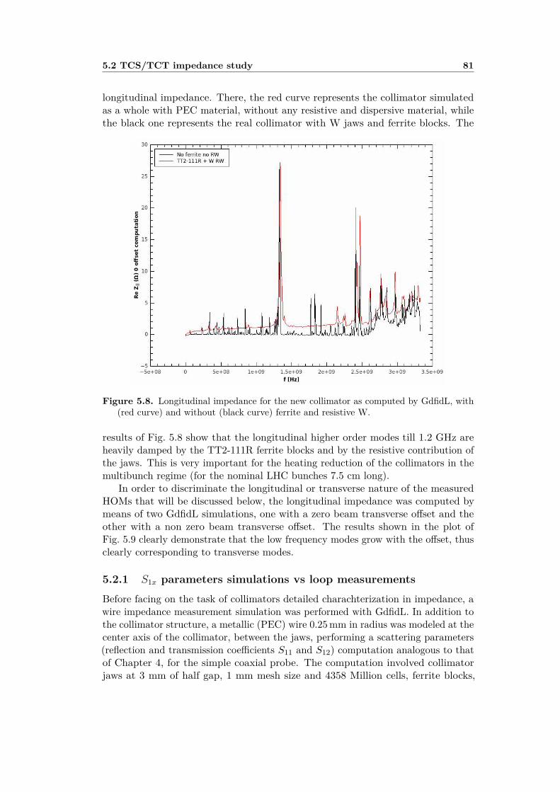
5.2 TCS/TCT impedance study 81
longitudinal impedance. There, the red curve represents the collimator simulatedas a whole with PEC material, without any resistive and dispersive material, whilethe black one represents the real collimator with W jaws and ferrite blocks. The
Figure 5.8. Longitudinal impedance for the new collimator as computed by GdfidL, with(red curve) and without (black curve) ferrite and resistive W.
results of Fig. 5.8 show that the longitudinal higher order modes till 1.2 GHz areheavily damped by the TT2-111R ferrite blocks and by the resistive contribution ofthe jaws. This is very important for the heating reduction of the collimators in themultibunch regime (for the nominal LHC bunches 7.5 cm long).
In order to discriminate the longitudinal or transverse nature of the measuredHOMs that will be discussed below, the longitudinal impedance was computed bymeans of two GdfidL simulations, one with a zero beam transverse o�set and theother with a non zero beam transverse o�set. The results shown in the plot ofFig. 5.9 clearly demonstrate that the low frequency modes grow with the o�set, thusclearly corresponding to transverse modes.
5.2.1 S1x
parameters simulations vs loop measurementsBefore facing on the task of collimators detailed charachterization in impedance, awire impedance measurement simulation was performed with GdfidL. In addition tothe collimator structure, a metallic (PEC) wire 0.25 mm in radius was modeled at thecenter axis of the collimator, between the jaws, performing a scattering parameters(reflection and transmission coe�cients S
11
and S12
) computation analogous to thatof Chapter 4, for the simple coaxial probe. The computation involved collimatorjaws at 3 mm of half gap, 1 mm mesh size and 4358 Million cells, ferrite blocks,

5.2 TCS/TCT impedance study 82
Figure 5.9. Longitudinal impedance for the new collimator, from longitudinal (zero beamo�set) simulation and from transverse dipolar (non zero beam o�set) simulation.
W IBC on all metallic surfaces and took 30 days on a 190 GB RAM, 32 cores, 4Socket Opteron 6370P Server (courtesy of W. Bruns). The results are shown inFig. 5.10(a), Fig. 5.10(b) and Table 5.7. While not resolved in the S
12
spectrum
GdfidL computed modesi f [ MHz]1 87.02 173.03 258.0
Table 5.7. Computed frequencies of the first three HOMs.
alone ( Fig. 5.10(a)), the HOMs are clearly distinguished in the power sum spectrum(Fig. 5.10(b)), the first three laying at the frequencies listed in Table 5.7. Compar-ing these latter with the frequencies of the HOMs measured at CERN with looptechnique [68], it came out already at this stage a very good agreement betweenthe numerical calculations of the HOMs frequency spectrum and the measurements,assessing GdfidL simulations as a very reliable tool for further detailed impedanceinvestigations.
5.2.2 Z‹ simulations versus wire measurementsThe transverse dipolar wakes and impedances of the LHC Run II TCS/TCT collima-tors’ real structures were finally calculated by means of GdfidL simulations, for 3 mmand 8 mm of jaws’ half gaps. Bearing in mind the aim at estimating the damping

5.2 TCS/TCT impedance study 83
(a)
(b)
Figure 5.10. (a) transmission coe�cient and (b) power sum of reflection and transmissioncoe�cients computed by means of the wire measurement GdfidL simulation.

5.2 TCS/TCT impedance study 84
Figure 5.11. HOMs spectrum of the Run II collimator, measured with the loop technique(courtesy of N. Biancacci, CERN).
features of the ferrite blocks on HOMs, both structures with and without dispersiveand properties of TT2-111R, but together with resistive W jaws, were considered.The results of such an extensive simulation campaign are shown in Fig. 5.12 andFig. 5.13.
The wake field was traced up to s = 200 m. It came out that in the case of 3 mmhalf gap collimator, the wake with only W exhibited a worst decay over the tracedwake length, with respect to the same computation for the case of 8 mm half gap(Fig. 5.12(a) and Fig. 5.13(a), respectively). In any case, a better wake decay wasassured by the ferrite blocks for both geometries, as theoretically expected.
The TT2-111R ferrite resulted to be very e�ective in damping the transverseparasitic modes also, for frequencies above 500 MHz. The modes at lower frequenciesare less damped, residual transverse HOMs at frequencies around 100 MHz and 200MHz, with non-negligible shunt impedances still existing. This is clearly visible inthe plots of Fig. 5.12(b) and Fig. 5.13(b). The confidence in GdfidL HOMs spectrumcomputation reliability, first dealt with in the previous section, was complied in thiscase also, with the calculated frequencies of the modes being in reasonable agreementwith the loop measurements. The results are reported in Table 5.8. The e�ect
half-gap [mm] HOMsw/ TT2-111R w/o TT2-111R
f [MHz] Rs
[M�/m] f [MHz] Rs
[M�/m]
3 82.6 2.913 93.4 4.370167.2 0.485 181.1 0.797
8 84.7 0.239 95.7 0.340169 0.029 193.9 0.170
Table 5.8
of ferrite results also in the shift of HOMs characteristic frequencies toward lowerones. As an example, for 8 mm half gap, the first HOM frequency shifts from ¥ 95MHz to ¥ 84.5 MHz, at exactly the same frequency measured experimentally atCERN with loop technique [68]. It is clear that the computed impedance spectrum

5.2 TCS/TCT impedance study 85
s [m]
(a)
f [Hz]3.5e+09
(b)
Figure 5.12. Transverse dipolar (a) wake and (b) real part of impedance spectrum of LHCRun II TCS/TCT collimators, with 3 mm of jaws’ half gap. The impedance plot insetlayer focuses on low frequency HOMs.

5.2 TCS/TCT impedance study 86
s [m]
(a)
f [Hz]3.5e+09
(b)
Figure 5.13. Transverse dipolar (a) wake and (b) real part of impedance spectrum of LHCRun II TCS/TCT collimators, with 8 mm of jaws’ half gap. The impedance plot insetlayer focuses on low frequency HOMs.

5.2 TCS/TCT impedance study 87
Figure 5.14. 1st HOM RS as a function of jaws’ half gap, as measured with wire techniqueand simulated in CST PS and GdfidL.
resolved very well the low frequency HOMs, whose characteristic frequencies arein excellent agreement with those found experimentally. Moreover, under thesesimulation circumstances, the computed shunt resistances of the first HOM at ¥ 84MHz, for the two considered jaws’ half gaps, is in remarkably agreement, within afactor of 2, with those measured experimentally with the wire technique at CERN[69]. This can be easily stated from Fig. 5.14, where the results from first HOMmeasurements, from CST PS and GdfidL simulations are plotted as a function ofthe jaws’ half gap. For instance, in the case of 8 mm half gap Rsim
s
¥ 237 k�/mand Rmeas
s
¥ 152 k�/m [70]. It is noteworthy to say that these small discrepanciesmay depend on several collimator design constraints, namely the gap between theplate where ferrite blocks are installed (HOMs’ frequencies can shifts of the orderof tens percents), the gap between collimator jaws and external tank (which cana�ect the HOMs’ R
s
) and also on the mesh and computed wake length. There aregood margins to be confident, however, that the results coming out from the GdfidLsimulations presented so far could be more accurate, i.e. closer to the physicalreality, with respect to both measurements and CST simulations. This because itis well known that wire measurements perturb the field pattern inside a cavity likestructure, leading to a broadening of the modes, in frequency, and to a lowering inR
s
. The CST simulations, moreover, were performed with simplified models of thecollimators, whereas the GdfidL ones with real models coming from CAD drawings,including all the structures’ details, as it was already stressed several times in thisthesis.

88
Chapter 6
LHC TDI collimators
The LHC injection protection system consists of a number of absorbers, aimed atintercepting the beam in case of failures of the LHC injection kicker magnets (MKI)[71]. It is going to be upgraded to prepare the higher intensity proton beam forthe HL-LHC, process foreseen to be finished in the LHC LS II (2018-2019). In thecase of MKI failures, the injection absorbers (TDIS) must be able to withstandthe impact of a full injection train consisting of 288 bunches. Several materials forthe absorber blocks are presently being considered, including di�erent grades ofboron nitride, graphite and carbon-reinforced-carbon, all having a low density, a lowcoe�cient of thermal expansion, a high strength and a low Young’s modulus [72].Up to now, graphite R4550 seems to be a good compromise in terms of availabilityof shapes, machinability, costs and performances.
The preliminary TDIS design, shown in Fig. 6.1, is composed of three modules ofequal length, containing di�erent absorber materials, the first two of low Z absorberblocks (graphite R4550) and the third one of higher Z materials. The transverse
Figure 6.1. Preliminary design of one TDIS module [72].
dimensions of the absorber blocks are reported in Table 6.1, specifying the length

6.1 TDI taper optimization study 89
of a single module with and without tapering. The taper dimensions on eitherside depend on impedance calculations. The two TDI presently installed in LHC,
Parameter ValueBlock height 54 mmBlock width 58 mmActive absorber length 1500 mmTapering length 100 mmTapering angle 10°Total absorber length 1700 mm
Table 6.1. Dimensions of TDIS absorbers.
indeed, contribute significantly to both longitudinal and transverse impedances. Itwas indeed experimentally observed, by means of dedicated measurements duringRun I [73, 74], beam induced heating causing high vacuum pressures that a�ectedthe background of the experiments. Thus a special care in the TDI design stageis needed, to minimize their impedances in view of the higher intensities plannedfor the LHC Run III and HL-LHC. This requires an impedance optimization studyaimed at reducing geometric and resistive contributions. Such a study is still anongoing work, even if several interesting results were obtained up to now, from adedicated impedance simulations’ campaign with GdfidL code.
6.1 TDI taper optimization studyThe TDI’s jaws presently installed in the LHC consist of one linear taper plus a sharpdiscontinuity, as shown in Fig. 6.2, where the GdfidL model is reported. In view of
Figure 6.2. Jaw’s geometry of the TDI presently installed in the LHC, as modeled intoGdfidL.
the needed upgrade discussed at the beginning of the chapter, the LHC collimation

6.1 TDI taper optimization study 90
team proposed a new taper geometry consisting of a simple linear flat taper, asshown in Fig. 6.3 for the GdfidL model, in order to avoid the strong impedance ofthe type step in - step out [29, 27] due to the sharp discontinuity. The possibility to
Figure 6.3. Linear jaw’s geometry of the TDI, as modeled into GdfidL.
minimize the impedance of a taper was studied in 2007 [75], by a nonlinear geometrydescribed by a function of the type
h(z) = hmin
[1 + zL(—≠ 12 ≠ 1)]2
, (6.1)
where h(z) is the varying half height, z the longitudinal variable, hmin
and hmax
thelower and upper height limits, L the taper length and — © h
max
h
min
. Such a geometrywas modeled into GdfidL, as shown in Fig. 6.4, and proposed as a substitute of boththe sharp and linear taper geometry for the TDI design upgrade. In all the above
Figure 6.4. Nonlinear jaw’s geometry of the TDI, as modeled into GdfidL.

6.2 TDIS’ real structures impedance study 91
taper GdfidL models, additional 10 cm in and out tubes were placed “ad-hoc”, toguarantee numerical stability of the computation.
Thus GdfidL simulations of geometric and RW transverse broad-band impedances,longitudinal and transverse loss factors, of the above TDI jaws were carried out,tracing the wake field over a length s = 75 cm, driving a beam with a bunchlength ‡
z
= 7.5 cm. The RW contributions were computed for the R4550 graphite.Simulations’ results are listed in Table 6.2, where the “NEW geometry” refers to thelinear one proposed by the LHC collimation team and the “Alternative geometry”to the nonlinear one, whose proposal originated from the study being describedhere. It is evident that, from the impedance point of view only, the best geometry
PRESENT geometry (linear flat taper + sharp discontinuity)PEC R4550 graphite (‡Œ = 7.64 · 104 S/m)
kÎ [V/C] 1.73 · 109 2.59 · 109
Z‹(0) [k�/m] 49.4 123.1k‹ [V/Cm] 5.32 · 1013 1.37 · 1014
NEW geometry (only longer and higher linear flat taper)PEC R4550 graphite (‡Œ = 7.64 · 104 S/m)
kÎ [V/C] 1.59 · 109 2.69 · 109
Z‹(0) [k�/m] 31.9 109.6k‹ [V/Cm] 3.46 · 1013 1.21 · 1014
Alternative geometry (non linear taper)PEC R4550 graphite (‡Œ = 7.64 · 104 S/m)
kÎ [V/C] 1.61 · 109 2.82 · 109
Z‹(0) [k�/m] 19.98 102k‹ [V/Cm] 2.09 · 1013 1.11 · 1014
Table 6.2. Resulting transverse impedance, longitudinal and transverse loss factors fromGdfidL simulations of the three jaws’ tapers geometries.
for TDI collimator taper is the non linear one. A significant reduction, indeed, ofa factor ¥ 2.5 in both zero frequency impedance and kick factor, with respect tothe present TDI geometry, is estimated for the geometric contributions. For theRW contribution, instead, the reduction accounts only for a factor ¥ 1.2. Thegeometrical longitudinal loss factor is observed to not change significantly, altough avery tiny increase of the longitudinal loss factor, of about 9%, is expected.
6.2 TDIS’ real structures impedance studyThe impedance study for the TDIS’ real structures is still an ongoing work. Never-theless, several interesting preliminary results have been obtained so far.
A first upgraded TDIS model was conceived by the CERN EN-MME department[76], whose CAD drawings are shown in Fig. 6.5. They represent a very complicatedstructure of about 3 m length, in which the jaws’ tapers have an elliptical roundgeometry. The reproduction of the corresponding STL files, again without anysemplification, into GdfidL is shown in Fig. 6.6. Any structural detail is very well

6.2 TDIS’ real structures impedance study 92
(a)
(b)
(c)
Figure 6.5. CAD drawings for the first upgraded model of the TDIS collimator.

6.2 TDIS’ real structures impedance study 93
resolved, even if a less fine mesh, with respect to the collimators simulated so far, of1 mm in x, y directions and 0.5 mm in z was used. Due to the very long design, with
(a)
(b)
Figure 6.6. GdfidL elaboration of the first upgraded CAD model of the TDIS collimator.
many gaps, flanges, pumps and pipe interconnections, it was possible up to now tocompute the geometric longitudinal impedance only, with the available computingresources of EngPara, trancing the wake at most over a length s = 50 m. Theresults for the real part of the longitudinal impedance are plotted in Fig. 6.7(a),for the TDI with 25 mm of jaws’ half gap. They were quite encouraging already atthis stage. Dedicated impedance measurements with wire technique, performed atCERN, revealed indeed the presence of many harmful trapped modes [77].
A comparison of the simulated impedance with the experimental one shown inFig. 6.7, exhibit qualitatively a very similar impedance pattern. The measurementswere done on the whole TDI structure, including Hexagona Boron Nitride (hBN)coated blocks and the two Al+Cu and Cu blocks. The upper jaw was moved to≠2 mm below the geometrical center and the lower jaw to 12 mm, thus with a full gapof 10 mm. The simulated structure, on the other side, had an half gap of ±25 mm,thus a full gap of 50 mm. What is observed from the comparison in Fig. 6.7, is thata small impedance peak is computed at f ¥ 0.5 GHz, high narrow peaks in the range1 GHz / f / 1.1 GHz, a wider peak at f ¥ 1.5 GHz and broader peaks with smalleramplitudes at higher frequencies. This is an important result, given that a) thesimulations were performed for the geometric impedance only, while measurementswere done on the real collimator with all resistive and dispersive materials, b) themeasurements with wire technique can lead to HOMs frequencies shift toward highervalues and c) the HOMs tend to have lower frequencies for wider gaps.

6.2 TDIS’ real structures impedance study 94
(a)
(b)(b)
(c)
Figure 6.7. (a) TDIS geometric longitudinal impedance from GdfidL simulation, for 25 mmhalf gap, (b) TDIS longitudinal measurement experimental setup and (c) measurementresults.

6.2 TDIS’ real structures impedance study 95
(a)
(b) (c)
(d) (e)
Figure 6.8. CAD drawings for the second upgraded model of the TDIS collimator.
Figure 6.9. GdfidL elaboration of the second upgraded CAD model of the TDIS collimator.

6.2 TDIS’ real structures impedance study 96
A second upgraded TDIS design [76] was simulated, whose CAD drawings areshown in Fig. 6.8. The whole structure (Fig. 6.8(a)) was revised with respect tothe previous one, changing the jaws’ material of the first block only and leaving theother two blocks the same (Fig. 6.8(b) and Fig. 6.8(c)), modeling asymettrically theinput and output pipes (Fig. 6.8(d)) and leaving the jaws’ elliptical round taper onthe first block only, modifying the other two blocks with flat rectangular taper jaws(Fig. 6.8(e)). Moreover, the modules interconnections were were not oval anymore,but it was cut on one side due to specific request of the team computing the radiationto equipment and resulting potential damage [78]. A detailed view of the taperingregion, of the GdfidL simulated geometry, is shown in Fig. 6.9.
The geometric longitudinal wake field traced over a length of about 30 m and thecorresponding real and imaginary parts of the impedance are shown in Fig. 6.10 andFig. 6.11, respectively, together with the corresponding results for the first modeldiscussed before.
As a first comment, it is seen from Fig. 6.10 that in this second case it waspossible to obtain the wake field computed up to s ¥ 25 m only. This can probablyexplain the impedance HOMs splitting appearing at around 750 MHz. Both fromreal and imaginary parts of the impedance plotted in Fig. 6.11(a) and Fig. 6.11(b),however, it can be concluded that a significant improvement was achieved, from thegeometric longitudinal impedance point of view, with the new upgraded TDIS model.A loss factor reduction of ≥ 29% has been achieved in this case, as it resulted fromcomputations to be 7.14 ·1011 V/C for the first model and 5.04 ·1011 V/C for the newone. Moreover, the strong modes at around 1 GHz are heavily damped, but HOMsappear to be strongly damped at almost all frequencies, what is the most criticalgoal in view of the beam induced overheating reduction e�orts. Its overcoming bymeans of careful TDIS design, minimizing the impedance charachterizing it in detail,still deserves further investigations and dedicated extensive simulation campaigns.
Figure 6.10. Longitudinal wake field comparison for the first and second TDIS upgradedmodels.

6.2 TDIS’ real structures impedance study 97
(a)
(b)
Figure 6.11. Comparison between th longitudinal (a) real and (b) imaginary parts of theimpedance, for the first and second TDIS upgraded models.

98
Chapter 7
Conclusions
Numerical simulations of wake fields and impedances were carried out for 3 di�er-ent kinds of LHC collimators: LHC Run I TCS/TCT collimators without BPMpickup buttons, LHC Run II TCS/TCT collimators with BPMs and TDI injectioncollimators, by means of GdfidL electromagnetic code. For the first time in thefield of impedance computations, a complete and detailed simulation campaign ofcollimators’ real structures, including the properties of real and lossy dissipative ma-terials (CFC and W resistive walls, TT2-111R ferrite). This task was accomplishedusing huge real CAD (STL) designs and the GdfidL parallelization on the CERNEngpara dedicated cluster. For this puropose several benchmark numerical tests wereperformed for resistive walls and TT2-111R ferrite, using parallel computing withGdfidL code engaging billions of mesh points. The performed numerical tests haveconfirmed that GdfidL reproduces very well the properties of the lossy dispersivematerials. The simulation test results for the resistive walls and the lossy ferritesare in a good agreement with available analytical formulae and the results of othernumerical codes and semi-analytical models.
For LHC Run I TCS/TCT collimators, the comparison of the transverse kickfactors calculated for five di�erent jaws’ half gaps, has shown that the geometricimpedance contribution is not negligible with respect to the resistive wall one. Thestudy has contributed to the refinement of the LHC impedance model, as a result ofthe geometrical collimator impedance accounting for approximately 30% of the totalLHC impedance budget, at frequencies close to 1 GHz.
For the LHC Run II TCS/TCT collimators, the numerical studies of theimpedance have shown that the longitudinal higher order modes till 1.2 GHz areheavily damped by the TT2-111R ferrite blocks and by the resistive contributionof the jaws. This is very important for the heating reduction of the collimators inthe multibunch regime (for the nominal LHC bunches 7.5 cm long). The transversemodes at low frequencies are less damped, there are still residual transverse HOMsat frequencies around 100 MHz and 200 MHz with non-negligible shunt impedances.The calculated frequencies of the modes are in remarkable agreement with the loopmeasurements. The shunt impedances of the modes obtained numerically agreewithin a factor of 2 with the experimental data of the wire measurements performedby the CERN impedance group. Moreover, the broad-band transverse impedance ofthe new double taper collimators are evaluated to be approximately by 20% higher

99
with respect to that of the single taper secondary collimators.The taper’s shape of the TDI collimator jaws was optimized, including the
geometric impedance and resistive walls. It was shown that, from the impedancepoint of view, the best geometry is the non linear one. A significant reduction inboth zero frequency impedance and kick factor, with respect to the present TDIgeometry, was calculated for both the geometric and resistive wall contributions,altough a tiny increase of the longitudinal loss factor is expected.
Detailed TDI’s real structure impedance study is still an ongoing work. Howevergood and encouraging preliminary results were gained already at this stage. Forinstance, computed HOMs’ pattern in geometrical longitudinal impedance is verysimilar to that found experimentally by means of wire measurements performedat CERN, taking into account the di�erent conditions between simulations andmeasurements. This is very important in view of the next detailed HOMs character-ization like that performed for Run II TCS/TCT collimators. For the second followup TDI model the simulations results show an estimated reduction of about 29% inthe loss factor, and a significantly reduced longitudinal impedance.

100
Appendix A
The linear accelerator model
A circular accelerator can be modeled as in Fig. 2.1, with the beam circulating insidea metallic vacuum chamber, of varying cross section, on a trajectory of circumference2fiR. Given the simple harmonic oscillators describing the unperturbed singleparticle motion, in the x, y, z directions with angular frequencies Ê
x0
, Êy0
andÊ
z0
, the tunes ‹x0
, ‹y0
and‹z0
can be defined as these frequencies divided by thesynchronous particle1 revolution frequency Ê
0
. It results, in general, ‹x0
, ‹y0
∫ 1and ‹
z0
π 1.All other particles’ motion is described in a six dimensional phase space, whose
coordinates are (x, xÕ, y, yÕ, z, ”). The coordinates xÕ = dx / ds and yÕ = dy / ds arethe slopes of the horizontal and vertical coordinates of the particle with respectto the reference orbit, whereas ” = �P/P is the relative momentum error of theparticle. The unperturbed equation of motions for single particles are
xÕÕ +3
‹x0
R
42
x = 0, (A.1)
yÕÕ +3
‹y0
R
42
y = 0, (A.2)
zÕ = ≠÷”, (A.3)”Õ = 0, for unbunched beams, (A.4)
”Õ = 1÷
3‹
s0
R
42
z, for bunched beams, (A.5)
where a prime indicates the derivative with respect to s. In the above equations theslippage factor has been defined as
÷ = – ≠ 1“2
, (A.6)
where – is the momentum compaction factor, usually positive in accelerator rings2,1With synchronous particle the reference particle O of Fig. 2.1 is concerned, which has exactly
the design energy and stays on the design orbit in the accelerator. Its trajectory is designated bythe coordinate s, which is a time variable.
2There are also rings for which – < 0, e.g. the Low Energy Antiproton Ring (LEAR) at CERN,where lower momentum particles have longer closed orbits or larger radial excursions than highermomentum particles. A negative momentum compaction factor does imply an imaginary transitionenergy, thus an always negative slippage factor and a ring always below transition.

101
and “ the relativistic Lorentz factor. The first two eqs. A.1 and A.2 describe thesimple harmonic property of the transverse betatron oscillations of the particles.Usually the transverse tunes are related to the transverse — functions of the machineoptics [28] as
‹x0
= R
—x
and ‹y0
= R
—y
, (A.7)
where 2fi—x,y
are the betatron oscillation wavelengths.For “ æ Œ, the slippage factor ÷ ¥ – and ÷ > 0. For “ < “
tr
© 1/Ô
–, knownas transition energy, ÷ becomes negative. The above condition is commonly referredto as “below transition” and is usually a property of low energy hadron rings, whilethe opposite one “ > “
tr
as “above transition”, mostly encountered in electron ringsand high energy proton rings, in which the particle velocity v ¥ c. At transition,÷ = 0, the particles’ dynamics in the longitudinal phase space freezes; under thiscircumstances the beam is most vulnerable to perturbations. When an acceleratoris operated below transition, any particle with an energy slightly higher than thereference one (” > 0) will have its longitudinal coordinate increasing with time,i.e. zÕ > 0. Above transition, instead, any particle with an energy higher then thereference one will slow down, with zÕ < 0, even if its velocity is higher than that ofthe synchronous particle. This phenomenon is called the negative mass e�ect andrelies on the fact that particles with higher energies, with respect to the synchronousparticle, must circulate in the accelerator on larger orbits.
The longitudinal synchrotron oscillation can be obtained combining eqs. A.3and A.5 for bunched beams,
zÕÕ +3
‹s0
R
42
z = 0, (A.8)
whereas it is trivial to mention that for unbunched beams no longitudinal focusingdoes occur.
Equations A.1-A.5 describe the linear accelerator model and the unperturbedmotions of beam particles. Let a perturbation a�ect, for example, the focusing inthe y direction, being the perturbation linear in y:
yÕÕ +3
‹y0
R
42
y = Ky. (A.9)
The perturbed motion can be described by a perturbed tune
‹2
y
= ‹2
y0
≠ KR2, (A.10)
from which it can be deduced that for small perturbation, |KR2| π ‹2
y0
, the tunehas shifted by an amount
�‹y
= ‹y
≠ ‹y0
= ≠KR2
2‹y0
. (A.11)
This result would have been identical in the case of a linear perturbation in x. Thequantity �‹ is known as tune shift and plays a crucial role in the study of collectivee�ects. For perturbations driven by collective electromagnetic fields, the tune shiftsare generally complex.

102
Appendix B
The GdfidL Finite Di�erencecode
GdfidL is a Finite Di�erence Time Domain (FDTD) code that solves approximatelyMaxwell’s equations by means of the curl operators discretization. For homogeneousmaterials the process follows the Yee’s algorithm [79]. For non homogeneous dielectricor permeable materials, the discretization is performed based on the Weiland method[80]. The program is composed of two field solvers, one that computes resonantfields in loss-free structures and the other that computes time dependent fields,scattering parameters and wake potentials in lossy or loss-free structures [81]. Itsmain advantage is the grid cells being needed only in regions which are not filled withelectric or magnetic conducting materials, what has as a consequence a reduction inmemory and CPU usage.
The discretization of the curl operators allows to compute the time derivative ofa field component in a grid, from the values of the four sorrounding dual components.Let each field component in the computational volume have a triple index i, j, k,the resulting di�erence equations in loss-free regions are approximated as (here thed
dt
Hz
component is taken as an example)
ddt
H i,j,k
z
¥�
x
(Ei+1,j,k
x
≠ Ei,j,k
x
) + �y
(Ei+1,j,k
y
≠ Ei,j,k
y
)�
x
�y
. (B.1)
Despite of being quite simple to implement in a computer code, this di�erenceequation has the disadvantage of assigning grid cells also to regions where thematerial is ideal conducting, what makes managing computational volumes, in whichmany geometries are present, particularly resource demanding.
The approach of GdfidL is quite di�erent. Instead of using a triple index toidentify a field component in the computational volume, the indices n+
x
(l) and n+
y
(l)are introduced, for the neighbour cell in the positive x or y directions of the l ≠ thcell, as in Fig. B.1. Thus the equation for the d
dt
Hz
field component now reads
ddt
H l
z
¥�
x
(En
+x
(l)
x
≠ El
x
) + �y
(En
+y
(l)
y
≠ El
y
)�
x
�y
. (B.2)
Let h and e be arithmetic vectors denoting the discrete electomagnetic degrees offreedom (i.e. all the field components of E and H), then the equations for all the

103
Figure B.1. The l ≠ th gridcell with its six field components. Additionally the two fieldcomponents of neighbour cells are shown, which are needed to compute the curl of E atthe position of H l
z (the field components of H are denoted by B in this picture) [81].
components of H in the computational volume, similar to eq. B.2, can be written inmatrix form as
ddt
h = ≠Cee (B.3)
and, for d
dt
E, asddt
e = [‘]≠1Ch[µ]≠1h = Chúh. (B.4)
Once the curl operators have been discretized, the fields in the time domain arecomputed at the next timestep from the previous fields, on the basis of the leap frogscheme [79].
Resonant fields, instead, are computed by GdfidL solving an eigenvalue problemderived directly from eqs. B.3 and B.4. 1 Substituting h given by eq. B.3 into eq. B.4and taking the Fourier harmonic of the time derivative, the equation describing thealgebraic eigenvalue problem is found to be:
≠ ChúCee = ≠Ê2e. (B.5)
The lowest nonzero eigenvalues and their corresponding eigenvectors are found withthe algorithm by Tückmantel [82].
The S-parameters GdfidL computation proceeds performing a time domainsimulation and then a Fourier transform of the histories of the tangential fields at the
1Resonant fields can be computed by exciting a structure with a broadband pulse, then examiningthe ringing of the fields. But such an approach can be valid only if a good resolution in frequency isnot demanded, given this latter requiring a long simulation time, as �f = 1/T .

104
ports of the structure. At the locations where the waveguide crosses the boundaryof the computational volume, Absorbing Boundary Conditions (ABCs) are applied.They are implemented into the code as orthogonal functions which are the tangentialfields of the TE, TM and TEM waveguides modes.
In order to compute wakepotentials, finally, a rigid beam is allowed to traversethe computational volume. For long range wakefields, ABCs must be applied wherethe beam enters and exits the cavity. The primary field of the charge, in this case,cannot be expanded in the waveguides modes. Thus, with known velocity of thecharge, the primary field at the ABCs is also known and can be subtracted from thetotal field. The scattered waves remaining can be expanded in orthogonal waveguidemodes.
As a concluding remark, generally the solution of di�erence equations di�erfrom the solution of the di�erential equations. There are two main sources of error,i.e. the approximation of the di�erential equation by a di�erence equation - for ahomogeneous mesh this error is proportional to the dquare of the mesh spacing -and the error due to the approximation of the material distribution. The coe�cientsof the di�erence equations depend on the material parameters. In the “staircase”approximation, constant material parameters are assumed in each cell of the grid.Better approximations use the prismatic cells. GdfidL implements a mesh-fillingthat is constructed by a boolean combination of prismatic fillings. The reason forsuch a choice is that the finite di�erence coe�cients for a field component dependonly on the material in the immediate vicinity of the edge where the component isdefined on. This guarantees a reduction of the frequency error by a factor of ten, ascompared to a prismatic filling [83].

105
Bibliography
[1] Lyndon Evans and Philip Bryant. Lhc machine. Journal of Instrumentation,3(08):S08001, 2008.
[2] Lyndon Evans. The large hadron collider. New Journal of Physics, 9(9):335,2007.
[3] Peter W. Higgs. Broken symmetries and the masses of gauge bosons. Phys.Rev. Lett., 13:508–509, Oct 1964.
[4] F. Englert and R. Brout. Broken symmetry and the mass of gauge vectormesons. Phys. Rev. Lett., 13:321–323, Aug 1964.
[5] Mike Lamont. Status of the lhc. Journal of Physics: Conference Series,455(1):012001, 2013.
[6] The LHCb collaboration. Observation of J/Âp Resonances Consistent withPentaquark States in �0
b
æ J/ÂK≠p Decays. Phys. Rev. Lett., 115(7):072001,2015.
[7] The ATLAS Collaboration. Observation of a new particle in the search for thestandard model higgs boson with the atlas detector at the lhc. Physics LettersB, 716(1):1 – 29, 2012.
[8] The ATLAS Collaboration. A particle consistent with the higgs boson observedwith the atlas detector at the large hadron collider. Science, 338(6114):1576–1582, 2012.
[9] The CMS collaboration. Observation of a new boson at a mass of 125 GeV withthe CMS experiment at the LHC. Phys. Lett., B716:30–61, 2012.
[10] The CMS collaboration. A New Boson with a Mass of 125 GeV Observed withthe CMS Experiment at the Large Hadron Collider. Science, 338:1569–1575,2012.
[11] European Strategy for Particle Physics, adopted by the CERN Council at aspecial session at ministerial level in Lisbon in 2006. http://cern.ch/council/
en/EuropeanStrategy/ESParticlePhysics.html.
[12] European Strategy for Particle Physics Update 2013, CERN-Council-S/106,adopted at a special session in the Brussels on 30 May 2013. http://cern.ch/
council/en/EuropeanStrategy/ESParticlePhysics.html.

Bibliography 106
[13] The HL-LHC collaboration. HL-LHC Preliminary Design Report Deliverable:D1.5. Technical report, 2014. CERN-ACC-2014-0300.
[14] E. Metral. Beam intensity limitations, Deliverable: D2.4. Technical report,2014. CERN-ACC-2014-0297.
[15] O. Brüning et al. LHC Design Report. Technical report, Geneva, 2004. CERN-2004-003.
[16] R.W. Assmann et al. Requirements for the LHC collimation system. Proceedingsof the 8th European Particle Accelerator Conference, pages 197–199, 2002.
[17] R.W. Assmann et al. An improved collimation system for the LHC. Proceedingsof the 9th European Particle Accelerator Conference, pages 536–538, 2004.
[18] R.W. Assmann. Collimation for LHC high intensity beams. Proceedings ofthe 46th ICFA Advanced Beam Dynamics Workshop on High-Intensity andHigh-Brightness Hadron Beams HB2010, pages 21–33, 2010.
[19] A. Bertarelli et al. The Mechanical Design for the LHC Collimators. Proceedingsof European Particle Accelerator Conference EPAC04, pages 545–547, 2004.LHC-PROJECT-REPORT-786.
[20] E. Metral et al. Transverse Impedance of LHC Collimators. Proceedings ofParticle Accelerator Conference PAC07, pages 2003–2005, 2007. CERN-LHC-PROJECT-REPORT-1015.
[21] N Mounet et al. Impedances of Two Dimensional Multilayer Cylindrical andFlat Chambers in the Non-Ultrarelativistic Case. Proceedings of the 46th ICFAAdvanced Beam Dynamics Workshop on High-Intensity and High-BrightnessHadron Beams HB2010, pages 353–357, 2010.
[22] A.W. Chao. Physics of Collective Beam Instabilities in High Energy Accelerators.Wiley, 1993.
[23] K.Y. Ng. Physics of Intensity Dependent Beam Instabilities. World Scientific,2005.
[24] Wolfgang K. H. Panofsky and Melba Phillips. Classical Electricity and Mag-netism. Addison-Wesley, 1962.
[25] K. L. F. Bane and P. L. Morton. Deflection by the image current and chargesof a beam scraper. Proceedings of the 1986 Linac Accelerator Conference, page490, 1986.
[26] P. Wilson. The Fundamental Theorem of Beam Loading. Technical report,1987. SLAC-PUB-4441.
[27] B. W. Zotter and S. A. Kheifets. Impedances and Wakes in High Energy ParticleAccelerators. World Scientific, 1998.
[28] S. Y. Lee. Accelerator Physics. World Scientific, 2013.

Bibliography 107
[29] L. Palumbo, V.G. Vaccaro, and M. Zobov. Wake fields and impedance. LNF-94-041-P, C93-09-20.6, 1994.
[30] F.J. Sacherer. A longitudinal stability criterion for bunched beams. IEEETransactions on Nuclear Science, 20(3):825–829, 1973.
[31] B. W. Zotter and F. J. Sacherer. Transverse instabilities of relativistic particlebeams in accelerators and storage rings. Conf.Proc., C761110:175–218, 1976.
[32] D. Boussard. Observation of microwave longitudinal instabilities in the CPS.Technical Report CERN/LAB/II/RF/75-2, CERN, Geneva, 1975.
[33] E. Keil and W. Schnell. Concerning longitudinal stability in the ISR. TechnicalReport CERN-ISR-TH-RF-69-48. ISR-TH-RF-69-48, CERN, Geneva, Jul 1969.
[34] K. W. Robinson. Stability of Beam in Radiofrequency Systems. TechnicalReport CEAL-1010, Cambridge Electron Accelerator, 1964.
[35] N. Mounet. The LHC Transverse Coupled-Bunch Instability. PhD thesis, EcolePolytechnique, Lausanne, Mar 2012. Presented 2012.
[36] G. Rumolo and F. Zimmermann. Electron cloud simulations: beam instabilitiesand wakefields. Phys. Rev. ST Accel. Beams, 5:121002, Dec 2002.
[37] J. F. Esteban Müller et al. Probing the LHC impedance with single bunches.Technical Report CERN-ATS-Note-2013-001 MD, Jan 2013.
[38] B. Salvachua et al. Results on nominal collimator settings MD at 4 TeV.Technical report, Jun 2012.
[39] N. Mounet et al. Beam stability with separated beams at 6.5 tev. In LHCBeam Operation Workshop Evian 17-20 December 2012, 2012.
[40] W. Bruns. http://www.gdfidl.de.
[41] Y. H. Chin. User’s Guide for ABCI. http://abci.kek.jp/abci.htm.
[42] G.V. Stupakov. Geometrical wake of a smooth taper. Part.Accel., 56:83–97,1996.
[43] Robert L. Gluckstern et al. Coupling impedance of beam pipes of generalcross-section. Phys.Rev., E47:656–663, 1993.
[44] G. Stupakov. Low Frequency Impedance of Tapered Transitions with ArbitraryCross Sections. Phys.Rev.ST Accel.Beams, 10:094401, 2007.
[45] R.W. Assmann et al. LHC Collimation: Design and Results from Prototypingand Beam Tests. pages 1078–1080., 2005.
[46] Kaoru Yokoya. Resistive wall impedance of beam pipes of general cross-section.Part.Accel., 41:221–248, 1993.
[47] A. Grudiev. Simulation of longitudinal and transverse impedances of trappedmodes in lhc secondary collimator. CERN AB-Note-2005-042, 2005.

Bibliography 108
[48] H. A. Day. Measurements and Simulations of Impedance Reduction Techniquesin Particle Accelerators. PhD thesis, Manchester U., 2013. Presented 28 Jun2013.
[49] B. Salvant. Impedance of the TCTP design. Presented at 12th TCTP designmeeting, 2011.
[50] N. Mounet et al. Impedance and instabilities. In LHC Beam Operation WorkshopEvian 2-4 December 2014, 2014.
[51] E. Metral. Initial estimate of machine impedance. (Milestone Report MS29,CERN-ACC-2014-0005), Jan 2014.
[52] N. Mounet et al. Transverse impedance in the HL-LHC era. Presented at the3rd Joint HiLumi LHC-LARP Annual Meeting, Daresbury, UK, 2013.
[53] D. Wollmann et al. Beam feasibility study of a collimator with in-jaw beamposition monitors. Nuclear Instruments and Methods in Physics ResearchSection A: Accelerators, Spectrometers, Detectors and Associated Equipment,768:62 – 68, 2014.
[54] S. Krinsky et al. Impedance of finite length resistive cylinder. Phys. Rev. STAccel. Beams, 7:114401, Nov 2004.
[55] Gennady Stupakov. Resistive wall impedance of an insert. Phys. Rev. ST Accel.Beams, 8:044401, Apr 2005.
[56] Y. Shobuda et al. Coupling impedances of a resistive insert in a vacuum chamber.Phys. Rev. ST Accel. Beams, 12:094401, Sep 2009.
[57] N. Biancacci et al. Impedance studies of 2d azimuthally symmetric devices offinite length. Phys. Rev. ST Accel. Beams, 17:021001, Feb 2014.
[58] CST Computer Simulation Technology AG.
[59] O. Frasciello et al. Wake fields and impedances calculations with GdfidL, MMMand CST for benchmarking purposes, 2014. Contributed talk at BE-ABPImpedance meeting, February 2nd, CERN, Geneva, Switzerland.
[60] H. Tsutsui et al. Transverse Coupling Impedance of a Simplified Ferrite LickerMagnet Model. Technical report, 2000. LHC-PROJECT-NOTE-234.
[61] H. Tsutsui. Some Simplified Models of Ferrite Kicker Magnet for Calculations ofLongitudinal Coupling Impedance. Technical report, 2000. CERN-SL-2000-004AP.
[62] L.D. Landau and E.M. Lifshitz. Electrodynamics of Continuous Media (SecondEdition Revised and Enlarged), volume 8 of Course of Theoretical Physics.Pergamon, Amsterdam, 1984.
[63] The Sage Developers. Sage Mathematics Software (Version 6.8), 2015.http://www.sagemath.org.

Bibliography 109
[64] R. Boni et al. Study of the parasitic mode absorbers for the Frascati „-factoryrf cavities. Technical Report LNF-93-014-P, INFN-LNF, Frascati, Apr 1993.
[65] S. Ramo, J. R. Whinnery, and T. Van Duzer. Fields and Waves in Communi-cation Electronics (3rd Edition). John Wiley & Sons, 1994.
[66] Frasciello O. et al. Geometric beam coupling impedance of LHC secondarycollimators. Nuclear Instruments and Methods in Physics Research Section A:Accelerators, Spectrometers, Detectors and Associated Equipment,http://dx.doi.org/10.1016/j.nima.2015.11.139.
[67] O. Frasciello et al. Present status and future plans of LHC collimators wakefields and impedance simulations, 2015. Contributed talk at BE-ABP Impedancemeeting, March 23rd, CERN, Geneva, Switzerland.
[68] N. Biancacci et al. Impedance bench measurements on TCTP collimator withferrite, 2014. Contributed talk at BE-ABP Impedance meeting, August 8th,CERN, Geneva, Switzerland.
[69] N. Biancacci et al. Impedance bench measurements on TCTP and SLACcollimators, 2014. Contributed talk at BE-ABP Impedance meeting, April 14th,CERN, Geneva, Switzerland.
[70] O. Frasciello et al. Beam coupling impedance of the new LHC collimators, 2015.Contributed talk at 101st National Congress of the Italian Physical Society(SIF), September 24th, Rome, Italy.
[71] J. Uythoven et al. Upgrades to the LHC injection and beam dumping systemsfor the HL-LHC project. In Proceedings of IPAC 2014.
[72] J. Uythoven et al. Injection protection upgrade for the HL-LHC. In Proceedingsof IPAC 2015.
[73] N. Mounet et al. Impedance e�ects on beam stability. In LHC Beam OperationWorkshop Evian 2011, 2011.
[74] J. Esteban Muller et al. Measurements of the LHC longitudinal resistiveimpedance with beam. Proceedings of the 48th ICFA Advanced Beam DynamicsWorkshop on High-Intensity and High-Brightness Hadron Beams HB2012, 2012.
[75] B. Podobedov and I. Zagorodnov. Impedance minimization by nonlinear taper-ing. In Proceedings of Particle Accelerator Conference PAC07, pages 2006–2008,Albuquerque, New Mexico, USA, 2007.
[76] B. Salvant and L. Gentini. Private communications.
[77] N. Biancacci. Update on the HL-LHC impedance budget, 2014. Contributedtalk at HL-LHC WP 2 Task 2.4 meeting, November 19th, CERN, Geneva,Switzerland.
[78] B. Salvant. Private communications.

Bibliography 110
[79] K. Yee. Numerical solution of initial boundary value problems involvingMaxwell’s equations in isotropic media. Antennas and Propagation, IEEETransactions on, 14(3):302–307, 1966.
[80] T. Weiland. Eine Methode zur Lösung der Maxwellschen Gleichungen fürsechskomponentige Felder auf diskreter Basis. Archiv für Elektrotechnik undÜbertragungstechnik, (Electronics and Communication), Band 31 (1977), Seiten116-120.
[81] W. Bruns. GdfidL: a finite di�erence program with reduced memory and CPUusage. In Proceedings of Particle Accelerator Conference, volume 2, pages2651–2653, 1997.
[82] Tückmantel, J. An improved version of the eigenvector processor SAP appliedin URMEL. Technical report, 1985. CERN-EF/RF-85-4.
[83] Bruns, W. GdfidL with generalized diagonal fillings and periodic boundaryconditions. http://www.gdfidl.de.