simulated and measured loss maps with lhc collimators at the
TRANSCRIPT
Simulated and Measured Loss Maps with LHC collimators at the SPS and LHC
CARE-HHH-APD BEAM’07 workshopOctober 1st-5th, 2007
CERN, Geneva, Switzerland
S. Redaelli, R. Assmann, C. Bracco, T. Weiler and G. Robert-Demolaize
CERN, AB department
S. Redaelli, BEAM’07, 02-10-2007 2
• Introduction• Loss studies for the LHC Simulation tools Performance of a perfect system Energy deposition studies• Imperfection models Jaw surface deformations Aperture alignment errors• Loss studies at the SPS Experimental layout Simulated versus measured losses• Conclusions
Outline of my talk
S. Redaelli, BEAM’07, 02-10-2007
Introduction
3
x 200!!
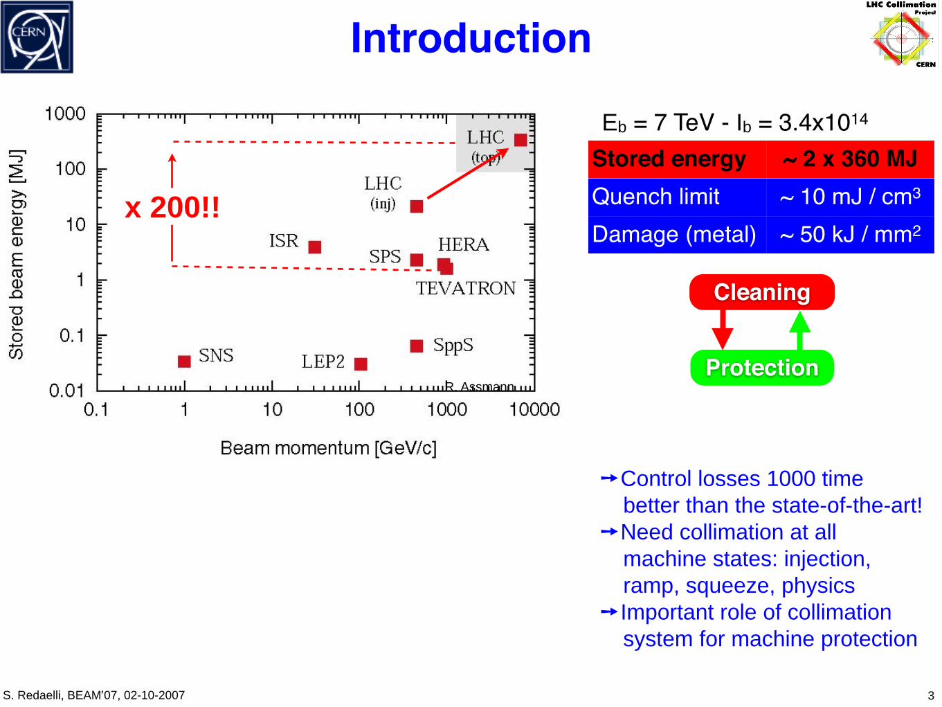
Stored energy ~ 2 x 360 MJQuench limit ~ 10 mJ / cm3
Damage (metal) ~ 50 kJ / mm2
➙Control losses 1000 time better than the state-of-the-art!
➙Need collimation at all machine states: injection, ramp, squeeze, physics
➙Important role of collimation system for machine protection
Cleaning
Protection
Eb = 7 TeV - Ib = 3.4x10¹⁴
R. Assmann

S. Redaelli, BEAM’07, 02-10-2007
Introduction
3
x 200!!
LHC enters in a new territory for handling ultra-intense beams in a super-conducting environment!Correspondingly, we need appropriate tools to understand the system performance!
Stored energy ~ 2 x 360 MJQuench limit ~ 10 mJ / cm3
Damage (metal) ~ 50 kJ / mm2
➙Control losses 1000 time better than the state-of-the-art!
➙Need collimation at all machine states: injection, ramp, squeeze, physics
➙Important role of collimation system for machine protection
Cleaning
Protection
Eb = 7 TeV - Ib = 3.4x10¹⁴
R. Assmann
S. Redaelli, BEAM’07, 02-10-2007
The Phase I LHC collimation system
4
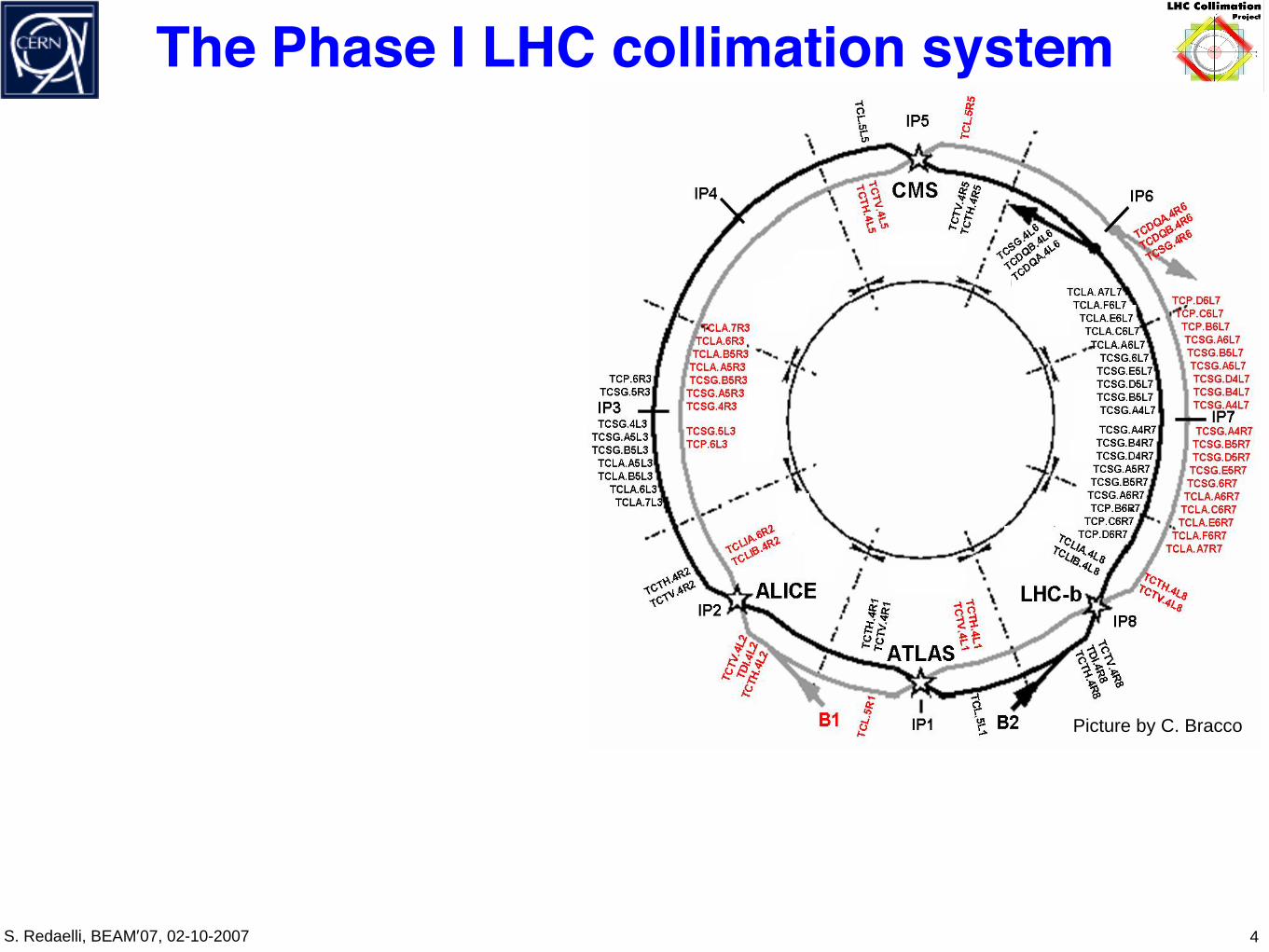
Picture by C. Bracco

S. Redaelli, BEAM’07, 02-10-2007
The Phase I LHC collimation system
4
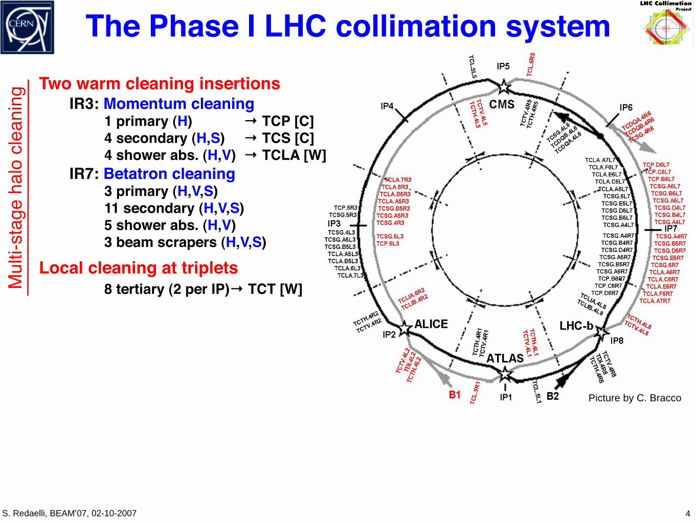
Two warm cleaning insertions IR3: Momentum cleaning 1 primary (H) → TCP [C] 4 secondary (H,S) → TCS [C] 4 shower abs. (H,V) → TCLA [W] IR7: Betatron cleaning 3 primary (H,V,S) 11 secondary (H,V,S) 5 shower abs. (H,V) 3 beam scrapers (H,V,S)
Picture by C. Bracco

S. Redaelli, BEAM’07, 02-10-2007
The Phase I LHC collimation system
4
Two warm cleaning insertions IR3: Momentum cleaning 1 primary (H) → TCP [C] 4 secondary (H,S) → TCS [C] 4 shower abs. (H,V) → TCLA [W] IR7: Betatron cleaning 3 primary (H,V,S) 11 secondary (H,V,S) 5 shower abs. (H,V) 3 beam scrapers (H,V,S)
Local cleaning at triplets 8 tertiary (2 per IP)→ TCT [W]
Picture by C. Bracco
S. Redaelli, BEAM’07, 02-10-2007
The Phase I LHC collimation system
4
Mul
ti-st
age
halo
cle
anin
g Two warm cleaning insertions IR3: Momentum cleaning 1 primary (H) → TCP [C] 4 secondary (H,S) → TCS [C] 4 shower abs. (H,V) → TCLA [W] IR7: Betatron cleaning 3 primary (H,V,S) 11 secondary (H,V,S) 5 shower abs. (H,V) 3 beam scrapers (H,V,S)
Local cleaning at triplets 8 tertiary (2 per IP)→ TCT [W]
Picture by C. Bracco

S. Redaelli, BEAM’07, 02-10-2007
The Phase I LHC collimation system
4
Mul
ti-st
age
halo
cle
anin
g Two warm cleaning insertions IR3: Momentum cleaning 1 primary (H) → TCP [C] 4 secondary (H,S) → TCS [C] 4 shower abs. (H,V) → TCLA [W] IR7: Betatron cleaning 3 primary (H,V,S) 11 secondary (H,V,S) 5 shower abs. (H,V) 3 beam scrapers (H,V,S)
Local cleaning at triplets 8 tertiary (2 per IP)→ TCT [W]
Physics debris absorbers [ Cu ] 2 TCLP’s (IP1/IP5)
Protection (injection/dump) 10 elements →TCLI/TCDQ [ C ]
Transfer lines 13 collimators → TCDI [ C ]
Passive absorbers for warm magnets
Picture by C. Bracco

S. Redaelli, BEAM’07, 02-10-2007
The Phase I LHC collimation system
4
Mul
ti-st
age
halo
cle
anin
g
44 movable ring collimators per beam
for the Phase I system!
Two warm cleaning insertions IR3: Momentum cleaning 1 primary (H) → TCP [C] 4 secondary (H,S) → TCS [C] 4 shower abs. (H,V) → TCLA [W] IR7: Betatron cleaning 3 primary (H,V,S) 11 secondary (H,V,S) 5 shower abs. (H,V) 3 beam scrapers (H,V,S)
Local cleaning at triplets 8 tertiary (2 per IP)→ TCT [W]
Physics debris absorbers [ Cu ] 2 TCLP’s (IP1/IP5)
Protection (injection/dump) 10 elements →TCLI/TCDQ [ C ]
Transfer lines 13 collimators → TCDI [ C ]
Passive absorbers for warm magnets
Picture by C. Bracco

S. Redaelli, BEAM’07, 02-10-2007
Multi-stage collimation at the LHC
5
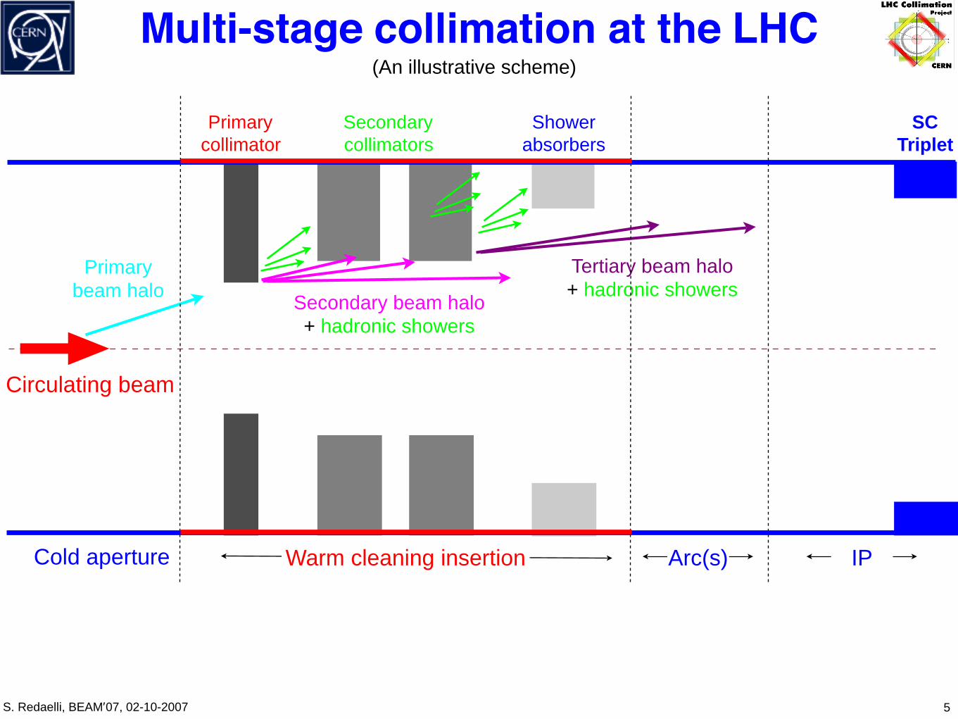
Cold aperture
Circulating beam
Warm cleaning insertion Arc(s) IP
(An illustrative scheme)

S. Redaelli, BEAM’07, 02-10-2007
Multi-stage collimation at the LHC
5
Cold aperture
Circulating beam
Primary beam halo
Warm cleaning insertion Arc(s) IP
(An illustrative scheme)

S. Redaelli, BEAM’07, 02-10-2007
Multi-stage collimation at the LHC
5
Cold aperture
Circulating beam
Primary beam halo
Primarycollimator
Secondarycollimators
Tertiary beam halo + hadronic showers
Secondary beam halo + hadronic showers
Warm cleaning insertion Arc(s) IP
(An illustrative scheme)

S. Redaelli, BEAM’07, 02-10-2007
Multi-stage collimation at the LHC
5
Cold aperture
Circulating beam
Primary beam halo
Primarycollimator
Secondarycollimators
Tertiary beam halo + hadronic showers
Secondary beam halo + hadronic showers
Shower absorbers
Warm cleaning insertion Arc(s) IP
(An illustrative scheme)
S. Redaelli, BEAM’07, 02-10-2007
Multi-stage collimation at the LHC
5
Cold aperture
Circulating beam
Primary beam halo
Primarycollimator
Secondarycollimators
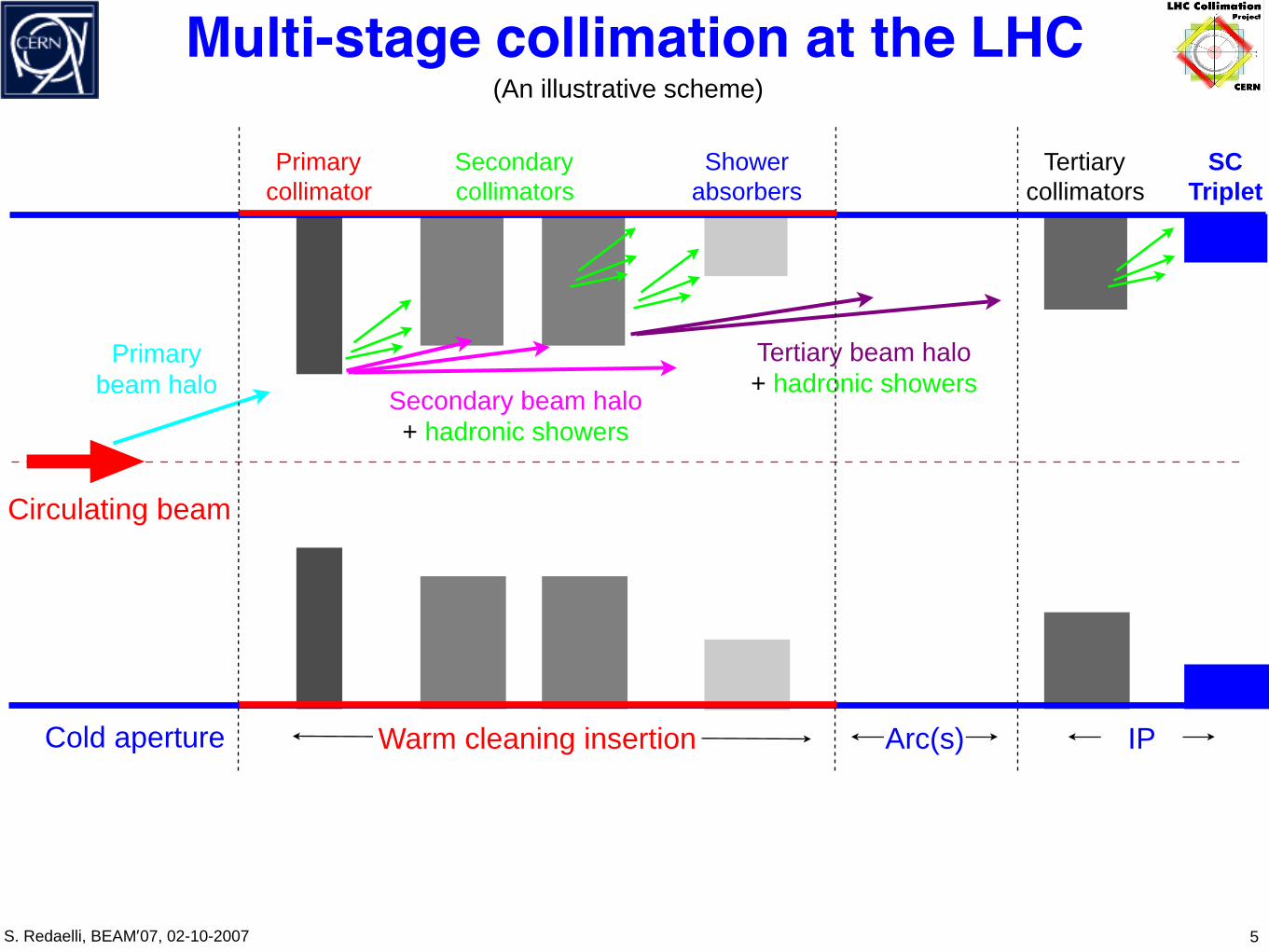
Tertiary beam halo + hadronic showers
Secondary beam halo + hadronic showers
Shower absorbers
Warm cleaning insertion
SCTriplet
Arc(s) IP
(An illustrative scheme)
S. Redaelli, BEAM’07, 02-10-2007
Multi-stage collimation at the LHC
5
Cold aperture
Circulating beam
Primary beam halo
Primarycollimator
Secondarycollimators
Tertiary beam halo + hadronic showers
Secondary beam halo + hadronic showers
Shower absorbers
Warm cleaning insertion
Tertiarycollimators
SCTriplet
Arc(s) IP
(An illustrative scheme)

S. Redaelli, BEAM’07, 02-10-2007
Multi-stage collimation at the LHC
5
Cold aperture
Circulating beam
Primary beam halo
Primarycollimator
Secondarycollimators
Tertiary beam halo + hadronic showers
Secondary beam halo + hadronic showers
Shower absorbers
Warm cleaning insertion
Tertiarycollimators
SCTriplet
Arc(s) IP
Protection devices
(An illustrative scheme)

S. Redaelli, BEAM’07, 02-10-2007
Multi-stage collimation at the LHC
5
Cold aperture
Circulating beam
Primary beam halo
Primarycollimator
Secondarycollimators
Tertiary beam halo + hadronic showers
Secondary beam halo + hadronic showers
Shower absorbers
Warm cleaning insertion
All cleaning + protection devices must be included in simulations!
Collimation needed from injection to collision!
Tertiarycollimators
SCTriplet
Arc(s) IP
Protection devices
(An illustrative scheme)

S. Redaelli, BEAM’07, 02-10-2007
Simulation tools for loss maps
6
S. Redaelli, BEAM’07, 02-10-2007
Simulation tools for loss maps
6
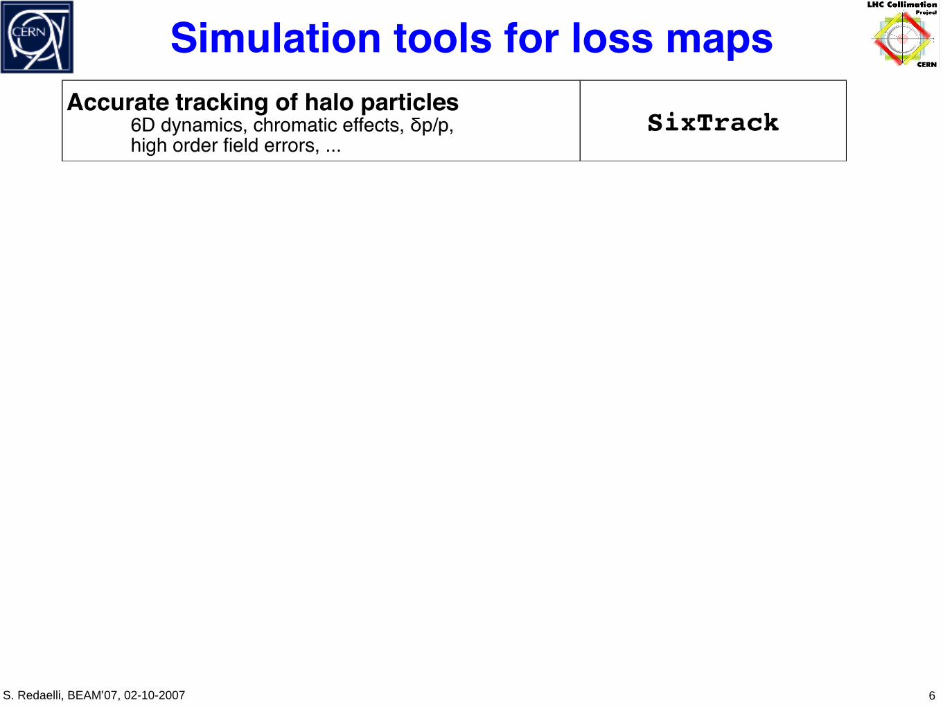
Accurate tracking of halo particles6D dynamics, chromatic effects, δp/p, high order field errors, ...
SixTrack

S. Redaelli, BEAM’07, 02-10-2007
Simulation tools for loss maps
6
Accurate tracking of halo particles6D dynamics, chromatic effects, δp/p, high order field errors, ...
SixTrack
Scattering routineTrack protons inside collimator materials K2

S. Redaelli, BEAM’07, 02-10-2007
Simulation tools for loss maps
6
Accurate tracking of halo particles6D dynamics, chromatic effects, δp/p, high order field errors, ...
SixTrack
Scattering routineTrack protons inside collimator materials K2
Detailed collimator geometryImplement all collimators and protection devices, treat any azimuthal angle, tilt/flatness errors
Detailed aperture model of full ringPrecisely find the locations of losses BeamLossPattern
20 20.5 21 21.5 22 22.5 23 23.5 24-0.2
-0.16-0.12-0.08-0.04
00.040.080.120.16
0.2
s [ km ]
Aper
ture
/ be
am p
ositio
n [ m
]
23.05 23.1 23.15 23.2 23.25 23.3 23.35-0.06
-0.04
-0.02
0
0.02
0.04
0.06
s [ km ]
Aper
ture
/ be
am p
ositio
n [ m
]
IR8
Magnet locations : ∆s ≤ 100m
Interpolation: ∆s=10cm(270000 points!)
0.02
0.03
0.04
Trajectory of a halo particle

S. Redaelli, BEAM’07, 02-10-2007
Example - one particle’s trajectory
• Scattering routine called within tracking at each collimator• If particle touches jaw, calculate absorption, offsets,
scattering angles and energy error• Trajectories of halo particles saved for off-line aperture
analysis (∆s < 10 cm)
19.78 19.8 19.82 19.84 19.86 19.88-80
-60
-40
-20
0
20
40
60
s [ km ]
X [ m
m ]
D3 D4 Q5.L7TCP TCS
LHC betatron cleaning (IR7)
(δx,δx’,δy,δy’,δE)
IR7→
Beam 1
(δx,δx’,δy,δy’,δE)
Incoming halo particle
Loss location

S. Redaelli, BEAM’07, 02-10-2007
Example - one particle’s trajectory
• Scattering routine called within tracking at each collimator• If particle touches jaw, calculate absorption, offsets,
scattering angles and energy error• Trajectories of halo particles saved for off-line aperture
analysis (∆s < 10 cm)
R.Assmann at al., LHC-PR 639 (2003)
TOOLS FOR PREDICTING CLEANING EFFICIENCY IN THE LHC
R. Aßmann, M. Brugger, M. Hayes, J.B. Jeanneret, F. Schmidt, CERN, Geneva, Switzerland
I. Baichev, IHEP, Protvino, Russia
D. Kaltchev, TRIUMF, Canada
Abstract
The computer codes Sixtrack and Dimad have been
upgraded to include realistic models of proton scattering
in collimator jaws, mechanical aperture restrictions, and
time-dependent fields. These new tools complement long-
existing simplified linear tracking programs used up to now
for tracking with collimators. Scattering routines from
STRUCT and K2 have been compared with one another
and the results have been cross-checked to the FLUKA
Monte Carlo package. A systematic error is assigned to
the predictions of cleaning efficiency. Now, predictions
of the cleaning efficiency are possible with a full LHC
model, including chromatic effects, linear and nonlinear er-
rors, beam-beam kicks and associated diffusion, and time-
dependent fields. The beam loss can be predicted around
the ring, both for regular and irregular beam losses. Exam-
ples are presented.
INTRODUCTION
The collimation system of the LHC [1] requires an excel-
lent cleaning efficiency in order to avoid quenches of the
super-conducting magnets. Various numerical tools used
for prediction of cleaning efficiency were compared. The
programs include generation of a primary beam halo, scat-
tering of high energy protons through material and tracking
of beam halos in the storage ring. The degree of agreement
between different codes is discussed. Differences are used
to assess possible systematic errors.
SCATTERING CODES
The physics of proton scattering in the material of col-
limator jaws has been implemented in various computer
codes. The scattering routines track the protons through
some length of a given material having them interacting
with the proper cross-sections. The protons receive trans-
verse kicks ∆θx, ∆θy and offsets ∆x, ∆y and some mo-mentum loss δ = ∆p/p0. Note that a full shower calcula-
tion is not required for predicting the cleaning of ”primary”
beam protons.
The primary protons in the LHC have energies from
450 GeV at injection to 7 TeV at top. The scattering rou-
tines must correctly describe the interactions over the full
range of energies, allow for different jaw materials, and in-
clude the correct jaw geometry, as protons impact at very
close distance from the edge of the jaw.
Three different scattering routines were compared:
1. K2 was developed in the 1990’s by Jeanneret and
Trenkler for studies of LHC collimation [2].
2. STRUCT was developed in the 1980’s by Baichev
et al, amongst others for studies of lHC and SSC collima-
tion [3].
3. FLUKA is a general purpose scattering and showering
code [4].
1e-006
1e-005
0.0001
0.001
0.01
0.1
-100 -80 -60 -40 -20 0 20 40 60 80 100
dN
/ (
dx
N0)
[µm
-1]
∆x [µm]
FLUKA
K2
STRUC
1e-006
1e-005
0.0001
0.001
0.01
-100 -80 -60 -40 -20 0 20 40 60 80 100
dN
/ (
dθ
x N
0)
∆θx [µrad]
FLUKA
K2
STRUC
[µ
rad
-1]
0.001
0.01
0.1
1
10
100
1000
0.001 0.01 0.1
dN
/ (
dδ N
0)
δ
K2FLUKA
STRUCT
Figure 1: Scattering probabilities for one 7 TeV proton im-
pacting on a 0.5 m long Cu jaw. Change in position (top),
angle (middle) and energy (bottom).
A test case was defined for the three routines: A 7 TeV
pencil beam with zero angle (y′ = 0) impacting y = 1µmfrom the edge of a 0.5 m long vertical collimator, made of
Cu. The changes in particles offsets, angles, and momen-
tum were recorded. The comparison of the different scat-
19.78 19.8 19.82 19.84 19.86 19.88-80
-60
-40
-20
0
20
40
60
s [ km ]
X [ m
m ]
D3 D4 Q5.L7TCP TCS
LHC betatron cleaning (IR7)
(δx,δx’,δy,δy’,δE)
IR7→
Beam 1
(δx,δx’,δy,δy’,δE)
1 case study: Three halo planes (Hori., vert. and skew); both beams.Track 5000000 particles for 200 turns.
Scattering in 44 collimators at each turn. Check the trajectory in 270000 aperture locations!
Incoming halo particle
Loss location

S. Redaelli, BEAM’07, 02-10-2007
Cleaning performance at 7 TeV
8
Beam1
Losses in collimators Losses in cold apert.
Beam2
Legend:Black = okayControlled losses at the collimators
Blue = BAD!Losses in cold aperture →quench
Only a few loss locations outside the collimators (ideal performance)
Betatron cleaning
(Nominal intensity, ideal performance, τb=0.2h)

S. Redaelli, BEAM’07, 02-10-2007
Details of beam 1 losses, 7 TeV
9
0 5 10 15 20 25 30
106
107
108
109
1010
1011
Longitudinal coordinate, s [ m ]
Loss
rate
per
uni
t len
gth
[ p/m
/s ]
IP2 IP3 IP4 IP5 IP6 IP7 IP8 IP1
Beam 1
(Nominal intensity, ideal performance, τb=0.2h)
By design, losses are concentrated in the warm insertion.
However, there is some leakage (~10-4): losses in the dispersion suppressor from single diffractive interaction with primary collimators.
This limits the Phase I performance.

S. Redaelli, BEAM’07, 02-10-2007
Details of beam 1 losses, 7 TeV
9
0 5 10 15 20 25 30
106
107
108
109
1010
1011
Longitudinal coordinate, s [ m ]
Loss
rate
per
uni
t len
gth
[ p/m
/s ]
IP2 IP3 IP4 IP5 IP6 IP7 IP8 IP1
Beam 1
-20 -10 0 10 20
-20
-10
0
10
20
Y [
mm
]
X [ mm ]
Sloss: s1=20290m; s2=20300m.Nloss = 304
(Nominal intensity, ideal performance, τb=0.2h)
By design, losses are concentrated in the warm insertion.
However, there is some leakage (~10-4): losses in the dispersion suppressor from single diffractive interaction with primary collimators.
This limits the Phase I performance.

S. Redaelli, BEAM’07, 02-10-2007
Cleaning performance at 450 GeV
10
0 5 10 15 20 25 30106
107
108
109
1010
1011
s [ km ]
Loss
rate
per
uni
t len
gth
[ p/m
/s ]
Assumed quench limit
IP2 IP3 IP4 IP5 IP6 IP7 IP8 IP1
(Nominal intensity, ideal performance, τb=0.1h)
Larger losses (larger betatron amplitudes at lower energy) but also larger quench limits.
Below the assumed quench limits!

S. Redaelli, BEAM’07, 02-10-2007
Cleaning during energy ramp
11
Beam cleaning needed throughout the ramp! Collimator settings: trade off between- Optimum cleaning Maintain canonical 6/7σ settings! σInj ≈ 1 mm → σ7TeV ≈ 0.25 mm- Ease operation in early commissioning Keep injection settings until β-squeeze!

S. Redaelli, BEAM’07, 02-10-2007
Cleaning during energy ramp
11
C. Bracco
Beam cleaning needed throughout the ramp! Collimator settings: trade off between- Optimum cleaning Maintain canonical 6/7σ settings! σInj ≈ 1 mm → σ7TeV ≈ 0.25 mm- Ease operation in early commissioning Keep injection settings until β-squeeze!
Proposed optimized setting during energy ramp: Constant retraction in millimeters: easy tolerances + sufficient cleaning at startup with reduced intensities.Detailed commissioning scenarios worked out by C. Bracco (PhD work).
S. Redaelli, BEAM’07, 02-10-2007 12
Overview of energy deposition studies
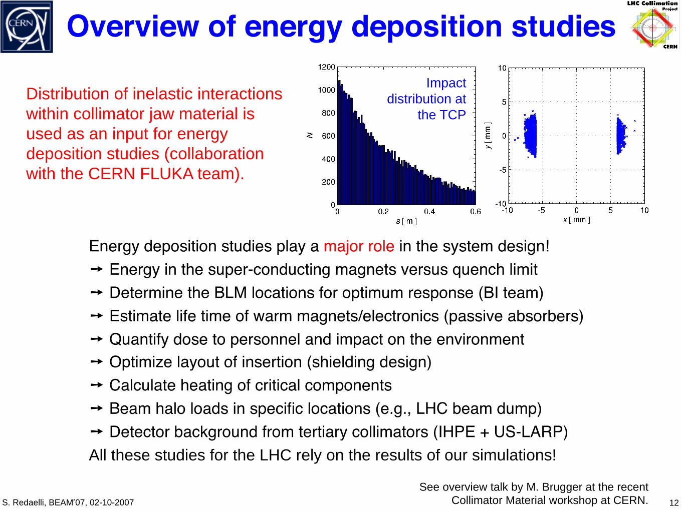
Energy deposition studies play a major role in the system design!➙ Energy in the super-conducting magnets versus quench limit➙ Determine the BLM locations for optimum response (BI team)➙ Estimate life time of warm magnets/electronics (passive absorbers)➙ Quantify dose to personnel and impact on the environment➙ Optimize layout of insertion (shielding design)➙ Calculate heating of critical components➙ Beam halo loads in specific locations (e.g., LHC beam dump)➙ Detector background from tertiary collimators (IHPE + US-LARP)All these studies for the LHC rely on the results of our simulations!
Distribution of inelastic interactions within collimator jaw material is used as an input for energy deposition studies (collaboration with the CERN FLUKA team).
Impact distribution at
the TCP
See overview talk by M. Brugger at the recent Collimator Material workshop at CERN.
S. Redaelli, BEAM’07, 02-10-2007
Radiation doses in IR7
13
- 8 -
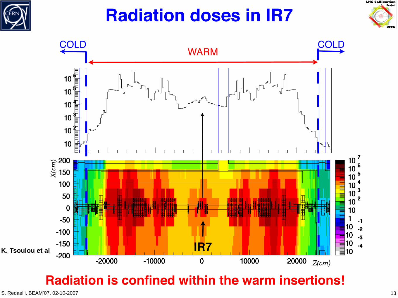
Figure 3 Dose rate distributions along the tunnel in Gy/year. The values shown are the
average of ±1m vertically from the beam line. In the upper figure the dose rate
distribution is plotted as a histogram and in the lower figure the same values are
shown in a contour plot together with the geometry. The regions of interest (RR73,
UJ76, RR77 – from left to right on the figure) are marked with the blue vertical
lines.
IR7
WARMCOLDCOLD
K. Tsoulou et al
Radiation is confined within the warm insertions!

S. Redaelli, BEAM’07, 02-10-2007
Radiation doses in IR7
13
- 8 -
Figure 3 Dose rate distributions along the tunnel in Gy/year. The values shown are the
average of ±1m vertically from the beam line. In the upper figure the dose rate
distribution is plotted as a histogram and in the lower figure the same values are
shown in a contour plot together with the geometry. The regions of interest (RR73,
UJ76, RR77 – from left to right on the figure) are marked with the blue vertical
lines.
IR7
WARMCOLDCOLD
5 or
ders
of m
agni
tude
!!
K. Tsoulou et al
Radiation is confined within the warm insertions!
S. Redaelli, BEAM’07, 02-10-2007
Optimization of the BLM locations
14
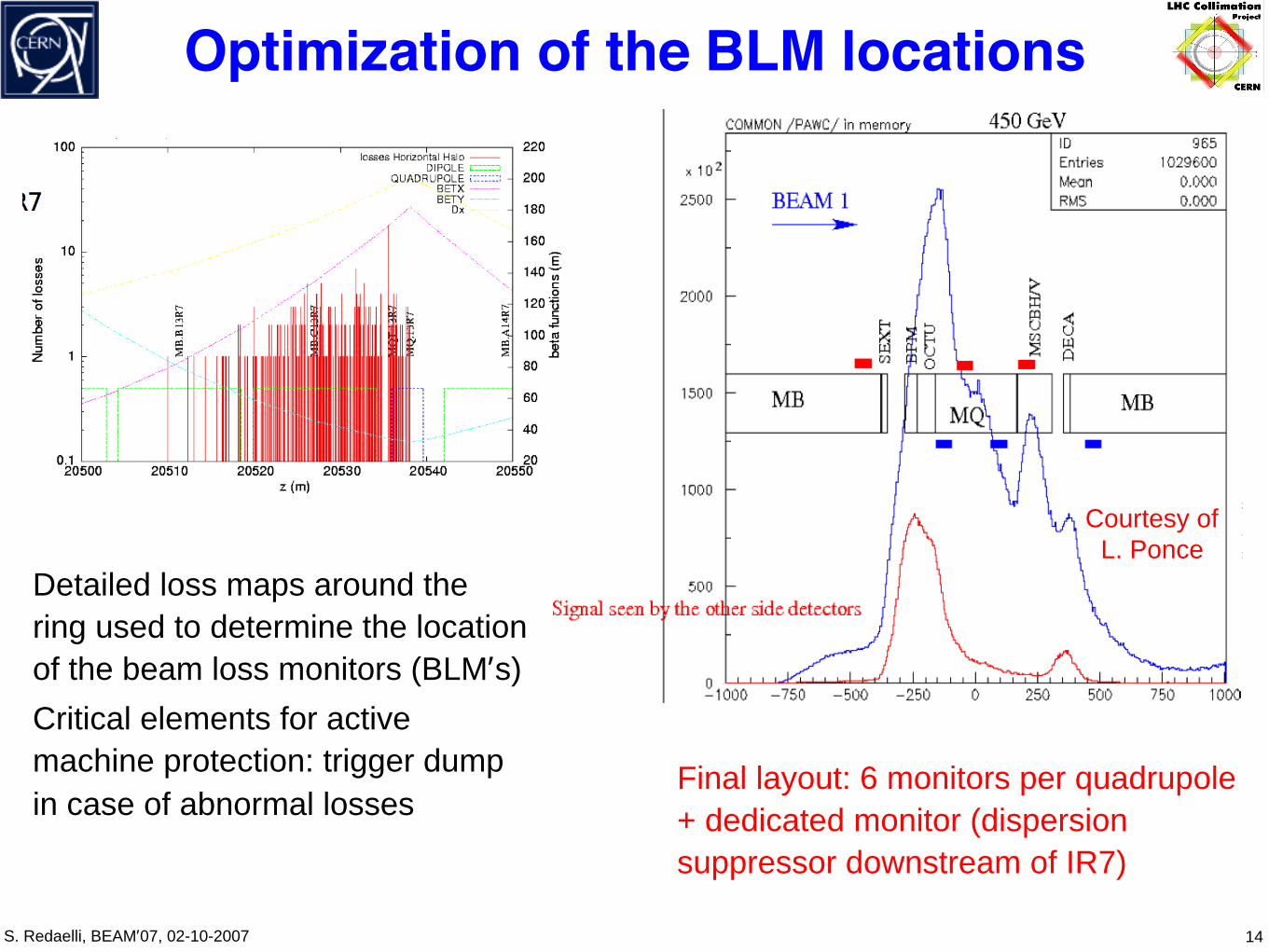
Courtesy of L. Ponce
Detailed loss maps around the ring used to determine the location of the beam loss monitors (BLM’s)
Critical elements for active machine protection: trigger dump in case of abnormal losses
Final layout: 6 monitors per quadrupole + dedicated monitor (dispersion suppressor downstream of IR7)

S. Redaelli, BEAM’07, 02-10-2007
Outline of my talk
15
• Introduction• Loss studies for the LHC Simulation tools Performance of a perfect system Energy deposition studies
• Imperfection models Jaw surface deformations Aperture alignment errors• Loss studies at the SPS Experimental layout Simulated versus measured losses• Conclusions

S. Redaelli, BEAM’07, 02-10-2007
Imperfection models - what can be wrong?
16

S. Redaelli, BEAM’07, 02-10-2007
Imperfection models - what can be wrong?
16
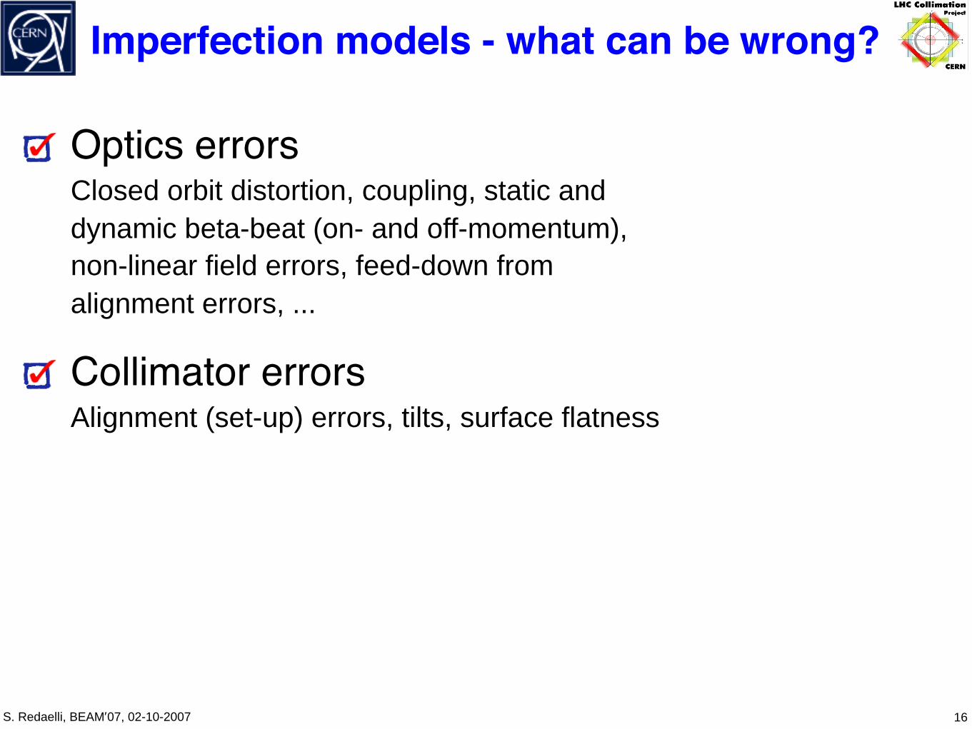
Optics errorsClosed orbit distortion, coupling, static and dynamic beta-beat (on- and off-momentum), non-linear field errors, feed-down from alignment errors, ...
S. Redaelli, BEAM’07, 02-10-2007
Imperfection models - what can be wrong?
16
Optics errorsClosed orbit distortion, coupling, static and dynamic beta-beat (on- and off-momentum), non-linear field errors, feed-down from alignment errors, ...
Collimator errorsAlignment (set-up) errors, tilts, surface flatness
Aperture imperfectionsStatistical errors, manufacturing errors, measured alignment, ...
Full MADX optics model implemented
in SixTrack
Detailed collimator geometry in our
scattering routine
Dedicated tools in aperture program

S. Redaelli, BEAM’07, 02-10-2007
0 2.0 4.0 6.0 8.0 15.1
2
5.2
3
5.3
4
5.4
5
] m [ Z ,etanidrooc lanidutignoL
Tran
sver
se c
oord
inat
e, X
[ m
m ]
Jaw flatness errors
17
Effect of flatness errors: - Halo particles interact with less material: → Reduced absorption!- More losses close to the downstream edge → More particles/showers escape- Higher deposited energy density
Collimator jaw bulk material
Beam
1m jaw (TCSG)
Perfect surface
0 2.0 4.0 6.0 8.0 15.1
2
5.2
3
5.3
4
5.4
5
Tran
sver
se c
oord
inat
e, X
[ m
m ]
] m [ Z ,etanidrooc lanidutignoL
Collimator jaw bulk material
“Banana” shape
Simulations: can slice each collimator and assign any shape (polynomial fit)Sensitivity studies + measured flatness from production
Error:250 μm

S. Redaelli, BEAM’07, 02-10-2007
Sensitivity on flatness errors
18
Based on these studies, the production tolerance was set to 40 μm.
Tolerance achieved in production. Database of flatness data being prepared to study the performance of the “as-built” system.
(parabolic “banana” deformation of all secondary collimators)
50 % lost of cleaning efficiency for errors of ~ 50 μmFactor 2-3 for errors above 250 μm

S. Redaelli, BEAM’07, 02-10-2007
Random aperture alignment errors
19
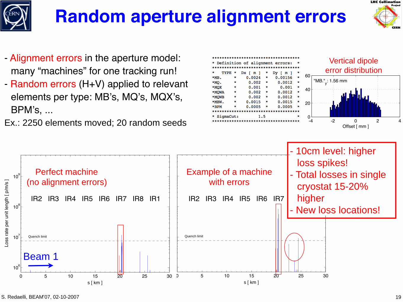
- Alignment errors in the aperture model: many “machines” for one tracking run!
- Random errors (H+V) applied to relevant elements per type: MB’s, MQ’s, MQX’s, BPM’s, ...
Ex.: 2250 elements moved; 20 random seeds
-4 -2 0 2 40
10
20
30
Offset [ mm ]
N
BLMx: 0.5 mm
-4 -2 0 2 40
10
20
30
Offset [ mm ]
N
BLMy: 0.5 mm
-4 -2 0 2 40
20
40
60
Offset [ mm ]
N
"MB."x: 2.4 mm
-4 -2 0 2 40
20
40
60
Offset [ mm ]
N
"MB."y: 1.56 mm
-4 -2 0 2 40
5
10
15
Offset [ mm ]N
"MQ."x: 2.0 mm
-4 -2 0 2 40
5
10
15
Offset [ mm ]
N
"MQ."y: 1.2 mm
Vertical dipole error distribution

S. Redaelli, BEAM’07, 02-10-2007
Random aperture alignment errors
19
- Alignment errors in the aperture model: many “machines” for one tracking run!
- Random errors (H+V) applied to relevant elements per type: MB’s, MQ’s, MQX’s, BPM’s, ...
Ex.: 2250 elements moved; 20 random seeds
-4 -2 0 2 40
10
20
30
Offset [ mm ]
N
BLMx: 0.5 mm
-4 -2 0 2 40
10
20
30
Offset [ mm ]
N
BLMy: 0.5 mm
-4 -2 0 2 40
20
40
60
Offset [ mm ]
N
"MB."x: 2.4 mm
-4 -2 0 2 40
20
40
60
Offset [ mm ]
N
"MB."y: 1.56 mm
-4 -2 0 2 40
5
10
15
Offset [ mm ]N
"MQ."x: 2.0 mm
-4 -2 0 2 40
5
10
15
Offset [ mm ]
N
"MQ."y: 1.2 mm
Vertical dipole error distribution
0 5 10 15 20 25 30106
107
108
109
s [ km ]
Loss
rate
per
uni
t len
gth
[ p/m
/s ]
Quench limit
Lowb - Coll - HORI - Perfect Aperture
0 5 10 15 20 25 30106
107
108
109
s [ km ]
Loss
rate
per
uni
t len
gth
[ p/m
/s ]
Quench limit
Alignment seed = 9
Beam 1
Perfect machine(no alignment errors)
Example of a machine with errors
IR2 IR3 IR4 IR5 IR6 IR7 IR8 IR1 IR2 IR3 IR4 IR5 IR6 IR7 IR8 IR1
- 10cm level: higher loss spikes!
- Total losses in single cryostat 15-20% higher
- New loss locations!

S. Redaelli, BEAM’07, 02-10-2007
Measured alignment errors
20
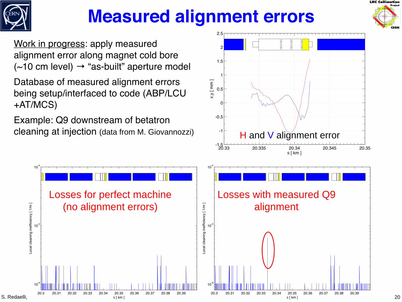
Work in progress: apply measured alignment error along magnet cold bore (~10 cm level) → “as-built” aperture modelDatabase of measured alignment errors being setup/interfaced to code (ABP/LCU+AT/MCS)Example: Q9 downstream of betatron cleaning at injection (data from M. Giovannozzi)
20.33 20.335 20.34 20.345 20.35-1.5
-1
-0.5
0
0.5
1
1.5
2
2.5
x,y
[ mm
]
s [ km ]
H and V alignment error
S. Redaelli, BEAM’07, 02-10-2007
Measured alignment errors
20
Work in progress: apply measured alignment error along magnet cold bore (~10 cm level) → “as-built” aperture modelDatabase of measured alignment errors being setup/interfaced to code (ABP/LCU+AT/MCS)Example: Q9 downstream of betatron cleaning at injection (data from M. Giovannozzi)
20.33 20.335 20.34 20.345 20.35-1.5
-1
-0.5
0
0.5
1
1.5
2
2.5
x,y
[ mm
]
s [ km ]
H and V alignment error
20.3 20.31 20.32 20.33 20.34 20.35 20.36 20.37 20.38 20.39
10-6
10-5
10-4
s [ km ]
Loca
l cle
anin
g in
effic
ienc
y [ 1
/m ]
20.3 20.31 20.32 20.33 20.34 20.35 20.36 20.37 20.38 20.39
10-6
10-5
10-4
s [ km ]
Loca
l cle
anin
g in
effic
ienc
y [ 1
/m ]
Losses for perfect machine(no alignment errors)
Losses with measured Q9 alignment

S. Redaelli, BEAM’07, 02-10-2007 21
• Introduction• Loss studies for the LHC Simulation tools Performance of a perfect system Energy deposition studies• Imperfection models Jaw surface deformations Aperture alignment errors• Loss studies at the SPS Experimental layout Simulated versus measured losses• Conclusions
Outline of my talk

S. Redaelli, BEAM’07, 02-10-2007
Layout of collimator tests at the SPS
22
A horizontal LHC collimator prototype (full mechanical
functionalities) installed in SS5 for beam tests.

S. Redaelli, BEAM’07, 02-10-2007
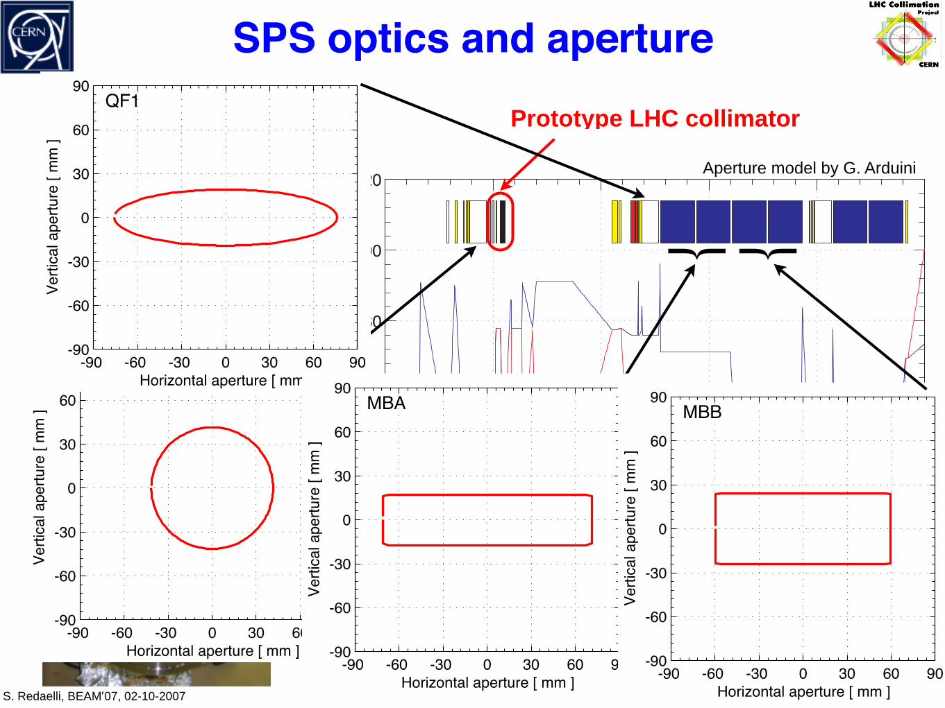
SPS optics and aperture
23
Prototype LHC collimatorMain beam parametersβx = 24.9m ➘ σx ≈ 0.7mm
βy = 89.9m ➘ σy ≈ 1.3mm
En = 270 GeV / cε ≈ 1-3 µm
Aperture model by G. Arduini

S. Redaelli, BEAM’07, 02-10-2007
SPS optics and aperture
23
Prototype LHC collimatorMain beam parametersβx = 24.9m ➘ σx ≈ 0.7mm
βy = 89.9m ➘ σy ≈ 1.3mm
En = 270 GeV / cε ≈ 1-3 µm
-90 -60 -30 0 30 60 90-90
-60
-30
0
30
60
90
Verti
cal a
pertu
re [
mm
]
Horizontal aperture [ mm ]
QD
Aperture model by G. Arduini

S. Redaelli, BEAM’07, 02-10-2007
SPS optics and aperture
23
Prototype LHC collimatorMain beam parametersβx = 24.9m ➘ σx ≈ 0.7mm
βy = 89.9m ➘ σy ≈ 1.3mm
En = 270 GeV / cε ≈ 1-3 µm
-90 -60 -30 0 30 60 90-90
-60
-30
0
30
60
90
Verti
cal a
pertu
re [
mm
]
Horizontal aperture [ mm ]
QD-90 -60 -30 0 30 60 90-90
-60
-30
0
30
60
90
Verti
cal a
pertu
re [
mm
]
Horizontal aperture [ mm ]
QF1
⎬
-90 -60 -30 0 30 60 90-90
-60
-30
0
30
60
90
Verti
cal a
pertu
re [
mm
]
Horizontal aperture [ mm ]
MBA
Aperture model by G. Arduini
S. Redaelli, BEAM’07, 02-10-2007
SPS optics and aperture
23
Prototype LHC collimatorMain beam parametersβx = 24.9m ➘ σx ≈ 0.7mm
βy = 89.9m ➘ σy ≈ 1.3mm
En = 270 GeV / cε ≈ 1-3 µm
-90 -60 -30 0 30 60 90-90
-60
-30
0
30
60
90
Verti
cal a
pertu
re [
mm
]
Horizontal aperture [ mm ]
QD-90 -60 -30 0 30 60 90-90
-60
-30
0
30
60
90
Verti
cal a
pertu
re [
mm
]
Horizontal aperture [ mm ]
QF1
⎬
-90 -60 -30 0 30 60 90-90
-60
-30
0
30
60
90
Verti
cal a
pertu
re [
mm
]
Horizontal aperture [ mm ]
MBA
-90 -60 -30 0 30 60 90-90
-60
-30
0
30
60
90
Verti
cal a
pertu
re [
mm
]
Horizontal aperture [ mm ]
MBB
⎬Aperture model by G. Arduini

S. Redaelli, BEAM’07, 02-10-2007
Generation and measurement of losses
24
Lifetime of SPS coasting beam: > 100h! How do we generate proton losses?
➙ Full or partial beam scraping with the collimator jaw!
Simulations were updated to include time-dependent
jaw movements: - 1 or 2 jaws can be moved at a speed of 2 mm/s - 20000 turns for the sweep across the beam

S. Redaelli, BEAM’07, 02-10-2007
Generation and measurement of losses
24
Lifetime of SPS coasting beam: > 100h! How do we generate proton losses?
➙ Full or partial beam scraping with the collimator jaw!
• One ionization chamber per quadrupole → Total of 36x6=216 BLM’s
• QD (smaller σx) have one H monitor and vice-versa• Losses integrated over 1 super-cycle of ~ 25 s
Ionization chamber
Simulations were updated to include time-dependent
jaw movements: - 1 or 2 jaws can be moved at a speed of 2 mm/s - 20000 turns for the sweep across the beam
S. Redaelli, BEAM’07, 02-10-2007
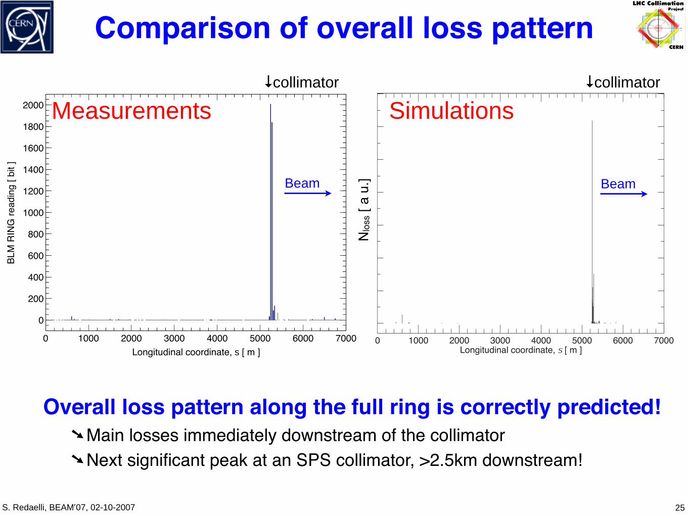
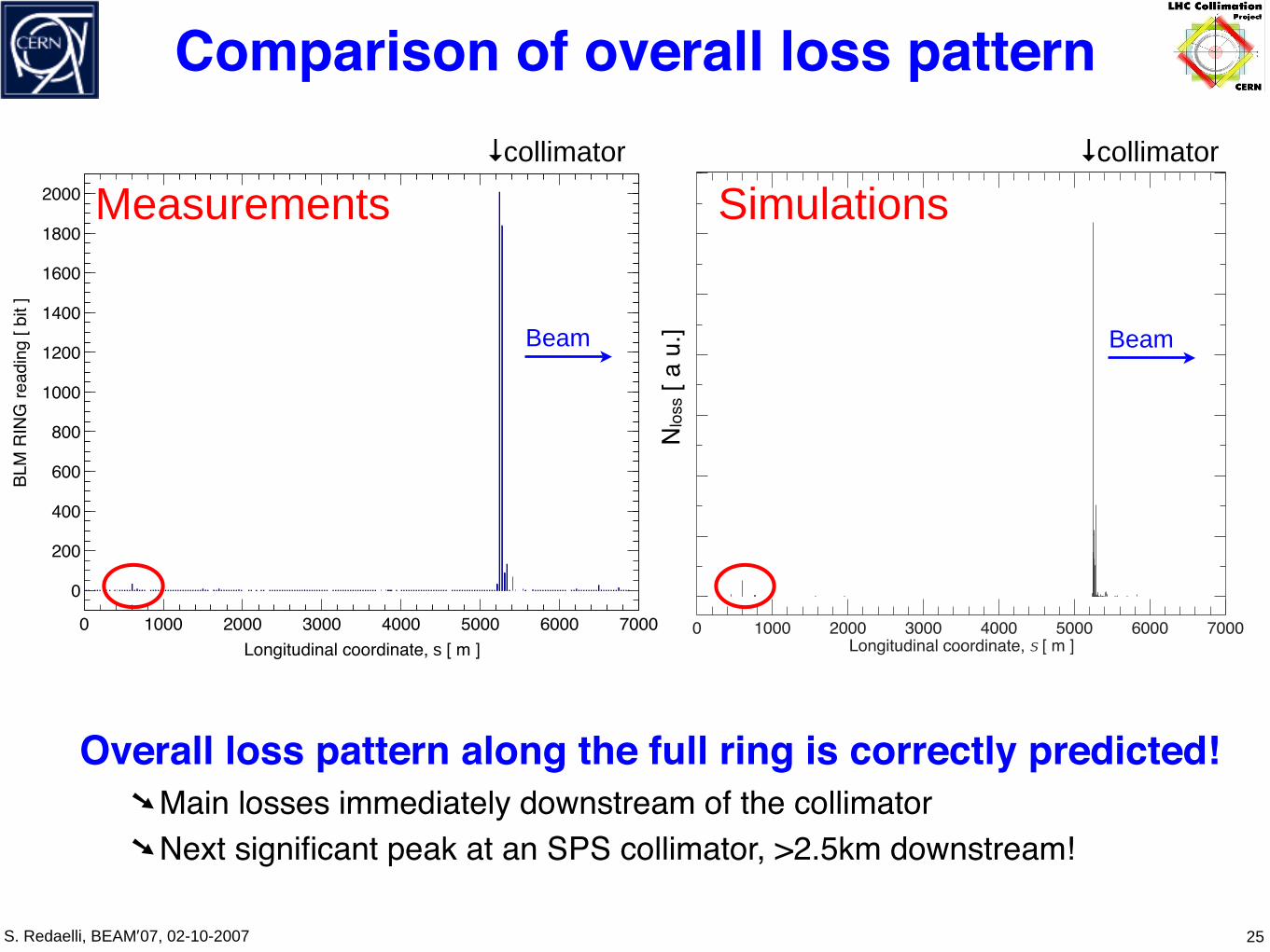
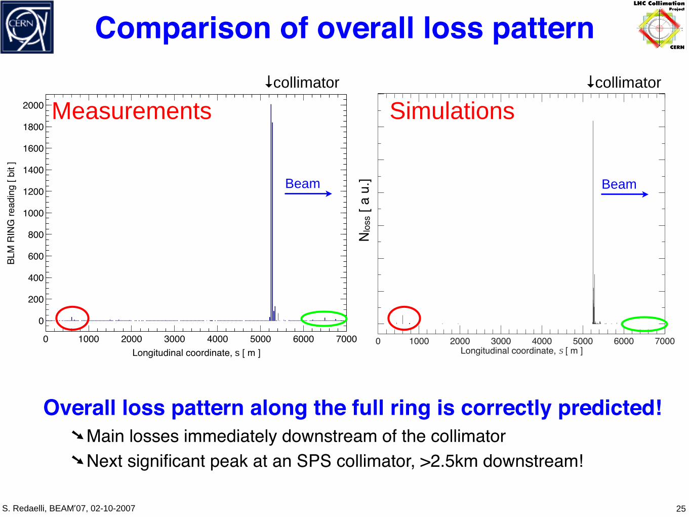
Comparison of overall loss pattern
25
0 1000 2000 3000 4000 5000 6000 7000
0
200
400
600
800
1000
1200
1400
1600
1800
2000
BLM
RIN
G re
adin
g [ b
it ]
Longitudinal coordinate, s [ m ]
SimulationsMeasurements
Overall loss pattern along the full ring is correctly predicted!➘Main losses immediately downstream of the collimator➘Next significant peak at an SPS collimator, >2.5km downstream!
Beam Beam
↓collimator ↓collimator
N los
s [ a
u.]
S. Redaelli, BEAM’07, 02-10-2007
Comparison of overall loss pattern
25
0 1000 2000 3000 4000 5000 6000 7000
0
200
400
600
800
1000
1200
1400
1600
1800
2000
BLM
RIN
G re
adin
g [ b
it ]
Longitudinal coordinate, s [ m ]
SimulationsMeasurements
Overall loss pattern along the full ring is correctly predicted!➘Main losses immediately downstream of the collimator➘Next significant peak at an SPS collimator, >2.5km downstream!
Beam Beam
↓collimator ↓collimator
N los
s [ a
u.]
S. Redaelli, BEAM’07, 02-10-2007 26
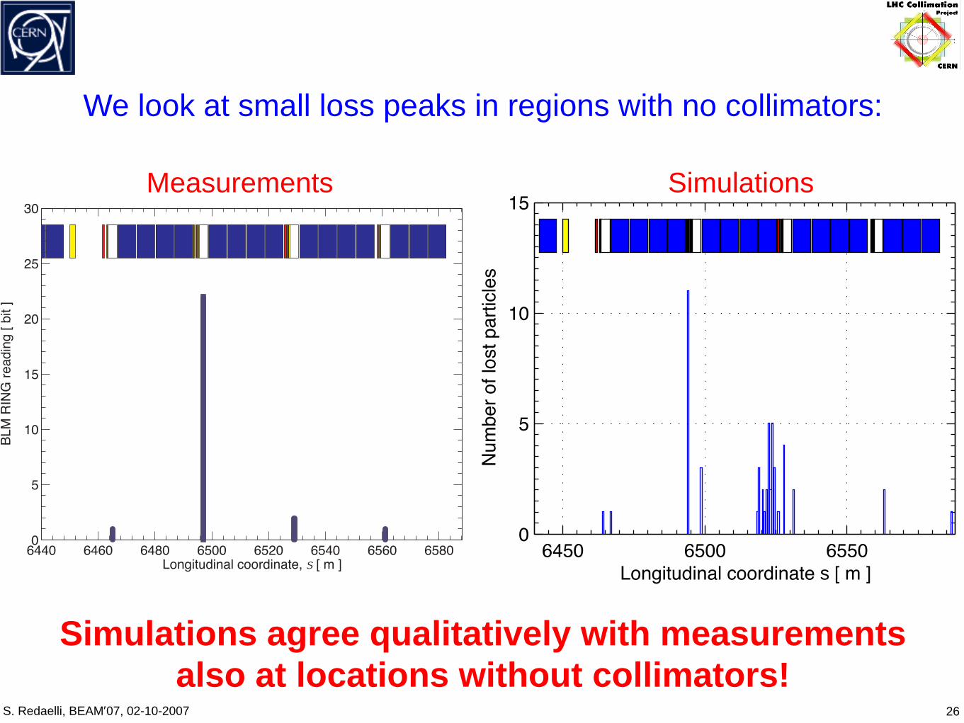
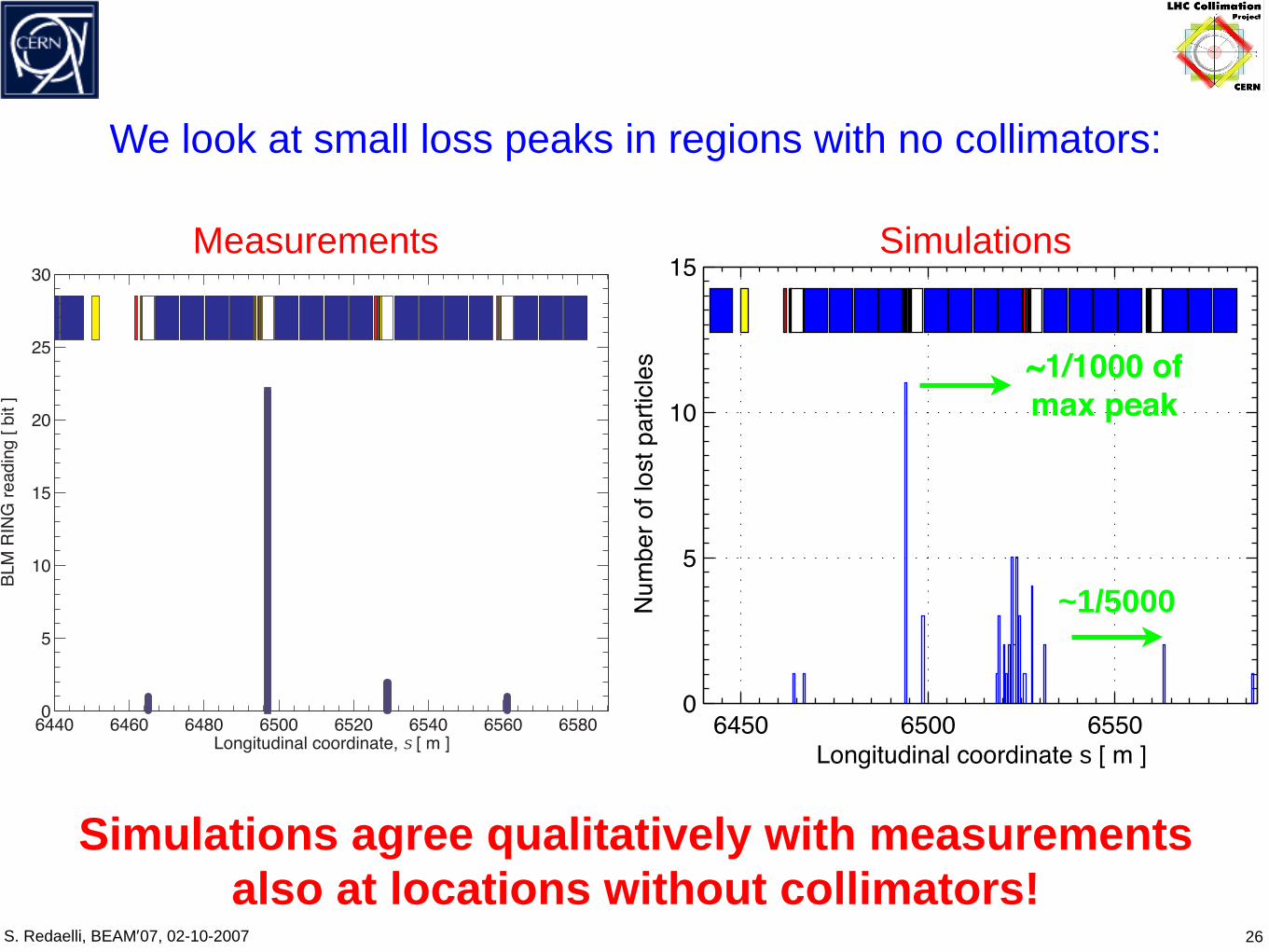
We look at small loss peaks in regions with no collimators:
6450 6500 65500
5
10
15
Longitudinal coordinate s [ m ]
Num
ber o
f los
t par
ticle
s
Measurements Simulations
Simulations agree qualitatively with measurements also at locations without collimators!
S. Redaelli, BEAM’07, 02-10-2007 26
We look at small loss peaks in regions with no collimators:
6450 6500 65500
5
10
15
Longitudinal coordinate s [ m ]
Num
ber o
f los
t par
ticle
s
Measurements Simulations
Simulations agree qualitatively with measurements also at locations without collimators!
~1/1000 of max peak
~1/5000

S. Redaelli, BEAM’07, 02-10-2007
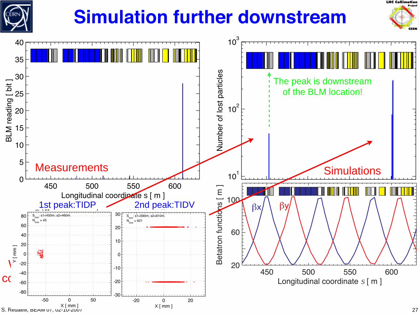
Simulation further downstream
27
450 500 550 600101
102
103
Num
ber o
f los
t par
ticle
s
Longitudinal coordinate s [ m ]450 500 550 600
0
5
10
15
20
25
30
35
40
BLM
read
ing
[ bit
]
Longitudinal coordinate s [ m ]
Measurements Simulations

S. Redaelli, BEAM’07, 02-10-2007
Simulation further downstream
27
450 500 550 600101
102
103
Num
ber o
f los
t par
ticle
s
Longitudinal coordinate s [ m ]450 500 550 600
0
5
10
15
20
25
30
35
40
BLM
read
ing
[ bit
]
Longitudinal coordinate s [ m ]
Measurements Simulations
The peak is downstream of the BLM location!
Difference understood if details of BLM mounting are taken into account!
We can nicely simulate losses but, of course, cannot measure without BLM’s!
-20 0 20-30
-20
-10
0
10
20
30
Y [
mm
]
X [ mm ]
Sloss: s1=590m; s2=610m.Nloss = 621
-50 0 50-80
-60
-40
-20
0
20
40
60
80
Y [
mm
]
X [ mm ]
Sloss: s1=450m; s2=460m.Nloss = 45
2nd peak:TIDV1st peak:TIDP

S. Redaelli, BEAM’07, 02-10-2007 28
• The simulation tools for LHC beam loss studies were presented• Codes evolved during the years to match the increasing complexity
of the LHC collimation system• Played a major role in the improvement of the final multi-stage
system from the original 2-stage cleaning• Detailed error models developed to understand the performance of
the realistic and “as-built” machine• Crucial importance for energy deposition and background studies• Tools are portable end documented on the web - extension to other
machines is straightforward!• Application to collimator induced beam loss at the SPS showed a
good agreement between simulations and measurements
Conclusions

S. Redaelli, BEAM’07, 02-10-2007 29
• AB-ABP-LCU members (M. Giovannozzi, W. Herr, S. Fartouhk)• AB/ATB members• F. Schimdt• J.B. Jeanneret• CERN BLM team• M. Jonker• SPS operation crew (G. Arduini, J. Wenninger)
Acknowledgments

S. Redaelli, BEAM’07, 02-10-2007 30
Reserveslides

S. Redaelli, BEAM’07, 02-10-2007
Beam halo loads in the dump region
31Energy deposition studies by L. Sarchiapone
Higher loss rates at the TCDQ for beam2
- Critical loss rates for beam 2: dump region immediately downstream of betatron cleaning
- Detailed simulation campaigns to investigate commissioning scenarios with reduced collimation system (C. Bracco, T. Weiler)
- Proposed additional shielding to achieve ultimate intensities

S. Redaelli, BEAM’07, 02-10-2007
Closed-orbit distortions
32
LHC tolerance: ± 4mm in arcs, ± 3mm in insertions.Scans of amplitude and phase of orbit errors to find critical spots. Extensive studies by G. Robert-Demolaize (PhD work).

S. Redaelli, BEAM’07, 02-10-2007
Improvements of the system
33There are still losses above the quench limit!
Full system with TCT’s + absorbers
2 stage cleaning in IR7 (as of Jan. 2005)
Beam
IP2 IP3 IP4 IP5 IP6 IP7 IP8 IP1
TCLA + TCT➙Significant improvement in the IR’s
Before ➙many losses outside collimators!

S. Redaelli, BEAM’07, 02-10-2007
Random aperture alignment errors
34
0 5 10 15 20 25 30106
107
108
109
s [ km ]
Loss
rate
per
uni
t len
gth
[ p/m
/s ]
Quench limit
Lowb - Coll - HORI - Perfect Aperture
0 5 10 15 20 25 30106
107
108
109
s [ km ]Lo
ss ra
te p
er u
nit l
engt
h [ p
/m/s
]
Quench limit
Alignment seed = 9
Perfect machine(no alignment errors)
Example of a machine with errors
20.25 20.3 20.35 20.4 20.45 20.5
106
107
108Lowb - Coll - HORI - Perfect Aperture
20.25 20.3 20.35 20.4 20.45 20.5
106
107
108Alignment seed = 9
Dispersion suppressor of IR7
Beam 1
1. Loss spikes at the 10cm level much higher (effect on quench performance to be understood)2. Total losses in single cryostat up to 15-20% higher3 .New loss locations!
S. Redaelli, BEAM’07, 02-10-2007
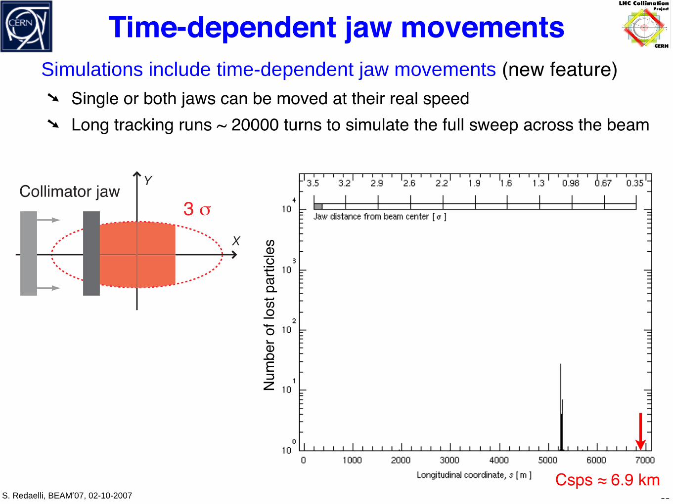
Time-dependent jaw movements
35
Simulations include time-dependent jaw movements (new feature) ➘ Single or both jaws can be moved at their real speed ➘ Long tracking runs ~ 20000 turns to simulate the full sweep across the beam
Csps ≈ 6.9 km
Num
ber o
f los
t par
ticle
s
S. Redaelli, BEAM’07, 02-10-2007
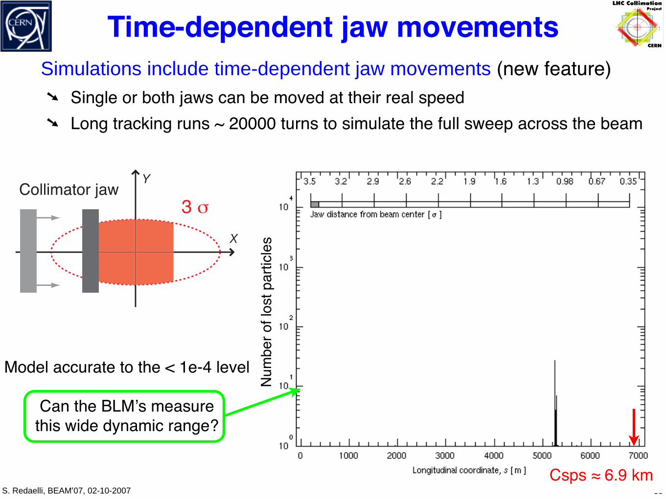
Time-dependent jaw movements
35
Simulations include time-dependent jaw movements (new feature) ➘ Single or both jaws can be moved at their real speed ➘ Long tracking runs ~ 20000 turns to simulate the full sweep across the beam
Model accurate to the < 1e-4 level
Can the BLM’s measure this wide dynamic range?
Csps ≈ 6.9 km
Num
ber o
f los
t par
ticle
s
S. Redaelli, BEAM’07, 02-10-2007
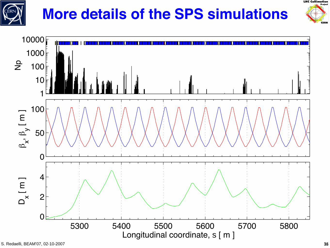
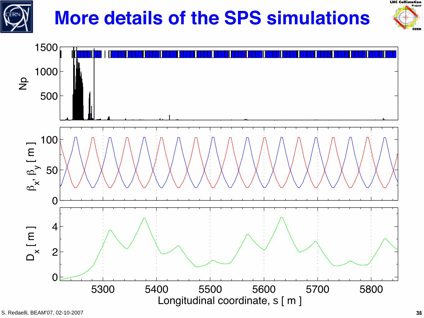
More details of the SPS simulations
36
110
1001000
10000
0
50
100
! x, !y [
m ]
5300 5400 5500 5600 5700 58000
2
4
Longitudinal coordinate, s [ m ]
D x [ m
]
11
Np

S. Redaelli, BEAM’07, 02-10-2007
More details of the SPS simulations
36
110
1001000
10000
0
50
100
! x, !y [
m ]
5300 5400 5500 5600 5700 58000
2
4
Longitudinal coordinate, s [ m ]
D x [ m
]
11
Dynamic range of BLM’s ?
Np
S. Redaelli, BEAM’07, 02-10-2007
More details of the SPS simulations
36
110
1001000
10000
0
50
100
! x, !y [
m ]
5300 5400 5500 5600 5700 58000
2
4
Longitudinal coordinate, s [ m ]
D x [ m
]
11
Dynamic range of BLM’s ?
500
1000
1500
0
50
100
! x, !y [
m ]
5300 5400 5500 5600 5700 58000
2
4
Longitudinal coordinate, s [ m ]
D x [ m
]Np
S. Redaelli, BEAM’07, 02-10-2007
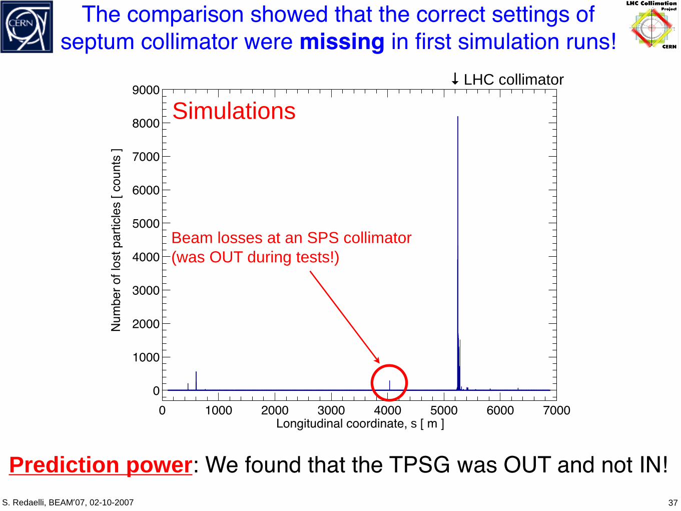
The comparison showed that the correct settings of septum collimator were missing in first simulation runs!
37
0 1000 2000 3000 4000 5000 6000 70000
1000
2000
3000
4000
5000
6000
7000
8000
9000
Num
ber o
f los
t par
ticle
s [ c
ount
s ]
Longitudinal coordinate, s [ m ]
Beam losses at an SPS collimator (was OUT during tests!)
Simulations
Prediction power: We found that the TPSG was OUT and not IN!
↓ LHC collimator