1

Towards data-driven car-following models

Vasileia Papathanasopoulou and Constantinos Antoniou*

National Technical University of Athens Zografou GR-15780, Greece

e-mail: vasileia.papathanasopoulou@gmail.com, antoniou@central.ntua.gr *corresponding author

ABSTRACT Car following models have been studied with many diverse approaches for decades. Nowadays, technological advances have significantly improved our traffic data collection capabilities. Conventional car following models rely on mathematical formulas and are derived from traffic flow theory; a property that often makes them more restrictive. On the other hand, data-driven approaches are more flexible and allow the incorporation of additional information to the model; however, they may not provide as much insight into traffic flow theory as the traditional models. In this research, an innovative methodological framework based on a data-driven approach is proposed for the estimation of car-following models, suitable for incorporation into microscopic traffic simulation models. An existing technique, i.e. locally weighted regression (loess), is defined through an optimization problem and is employed in a novel way. The proposed methodology is demonstrated using data collected from a sequence of instrumented vehicles in Naples, Italy. Gipps' model, one of the most extensively used car-following models, is calibrated against the same data and used as a reference benchmark. Optimization issues are raised in both cases. The obtained results suggest that data-driven car-following models could be a promising research direction. Keywords: Car-following models, Gipps' model, locally weighted regression (loess), machine learning methods, speed estimation, optimization, intelligent transportation systems, data-driven approaches

1. INTRODUCTION Simulation models allow the evaluation of traffic networks and are used as the fundamental tool of traffic management and safety research [Barceló, 2010]. Modeling traffic behavior has also contributed significantly to the development of Intelligent Transportation Systems (ITS) [Koutsopoulos and Farah, 2012]. According to the level of detail that traffic flow is modeled, simulation models may be classified as microscopic, mesoscopic and macroscopic. In microscopic models vehicles are described individually and interactions between vehicles or between vehicles and the road network are included [Bellemans et al., 2002]. Microscopic models include gap-acceptance, speed adaptation, lane changing, ramp merging, overtaking, and car-following models [Olstam and Tapani, 2004]. Each vehicle is described by parameters such as its origin, destination, desired speed, acceleration and deceleration, the type of vehicle and the

2

driver's characteristics [Bellemans et al., 2002]. Macroscopic traffic models use aggregated variables to describe traffic phenomena. Such models simulate the movement as a continuous flow, using theories often inspired by the fluid dynamics. Macroscopic measurements include speed, traffic flow and traffic density [Boxill and Yu, 2000]. Finally, mesoscopic models provide an intermediate situation, in which they model individual vehicles but at an aggregate level, usually using speed-density relationships and queuing models to model vehicle dynamics. Thus, mesoscopic models share common characteristics with both macroscopic and microscopic models [Boxill and Yu, 2000] and aim to combine the benefits of both, while overcoming their respective limitations.

An ongoing debate among traffic modelers relates to the relative benefits of each level of simulation models. The microscopic representation of traffic flow offers high accuracy at a computational cost and car following models are an essential component [Koutsopoulos and Farah, 2012; Brackstone and McDonald, 1999; Aycin and Benekohal, 1999]. The objective of this paper is not to enter this debate, but to provide an alternative modeling approach for car-following model within microscopic traffic simulation models. This modeling approach can take advantage of a wide range of available data, and is therefore suitable to implementation in the context of ITS systems. While microscopic traffic simulation models have a higher computational complexity, compared to mesoscopic or macroscopic models, they are more suited to the evaluation and operation of ITS, as they can model in detail more complex aspects of such systems. For example, it would be harder to model managed lanes, vehicle actuated traffic control systems and public transport priority systems with a mesoscopic or macroscopic model.

Car following models typically inspect driving behavior with respect to the preceding vehicle in the same lane. A vehicle is limited by the movement of the preceding vehicle, because driving at the desired rate may lead to a crash [Olstam and Tapani, 2004]. According to Olstam and Tapani [2004] car following models are divided into categories according to the logic used, such as Gazis-Herman-Rothery models [Gazis et al., 1961], safe distance models [Kometani and Sasaki, 1958; Gipps, 1981], psycho-physical models [Wiedermann and Reiter, 1992; Fritsche, 1994] and fuzzy logic models [Kikuchi and Chakroborty, 1992; Chakroborty and Kikuchi, 1999; Al-Shihabi and Morant, 2003].

Initially, car following models were developed to represent a single state of traffic, such as the traffic state, where the subject vehicle reacts to the actions of the preceding vehicle [Reuschel, 1950; Pipes, 1953]. Moreover, as Liu and Li [2013] mention, many of the earlier car following models, including the General Motors models [Chandler et al., 1958; Gazis et al., 1961] refer to low-speed situations and may not be suitable for high-speed networks. Recently, more and more researchers tend to adopt the concept that drivers behave differently in different traffic conditions [Yang and Koutsopoulos, 1996; Ahmed, 1999; Toledo, 2003; Wang et al., 2005; Koutsopoulos and Farah, 2012]. In this case, sub-phases can be recognized, such as free-flowing, approaching, close-following, car-following, emergency braking, and stop-and-go. This has led to the development of multi-regime car following models, according to which different rules are adopted under different traffic states, so that driving behavior can be best captured [Liu and Li, 2013].

A generalization of such multi-regime approaches is an attractive perspective. However, a large number of regimes may result to overly complex models and developing the equations to model them can become cumbersome. Furthermore, incorporating additional measurement data to these

3

models is very complicated. These restrictions have motivated us to suggest with this research an alternative methodology for the estimation of car-following models, combining flexible, data-driven components. Such methods have been used in several transport-related applications such as estimation or prediction of speed and classification of traffic data [e.g. Vlahogianni et al., 2005; van Lint, 2005, Antoniou and Koutsopoulos, 2006; van Lint, 2008; Vlahogianni et al., 2008; Dunne and Ghosh, 2012; Antoniou et al., 2013; Elhenawy et al., 2014]. Data-driven methods are more flexible than traditional models, allowing the incorporation of additional parameters, which influence driving behavior, thus leading to richer models.

Nowadays, the rapid development of technology has contributed to the availability of high-quality traffic data, leading the way for the development of more advanced car following models. Methods such as differential GPS and real time kinematic allow the collection of high fidelity traffic data [Ranjitkar et al., 2005] and consequently may improve the accuracy of traffic simulation models. On the other hand, ubiquitous sensors (e.g. accelerometers and gyroscopes) from regular smartphones could provide a much richer sample of heterogeneous data, which could allow much richer calibration, e.g. utilizing distributions rather than point values [Antoniou et al., 2014]. For a review of novel data collection techniques and their applications to traffic management applications see [Antoniou et al., 2011].

Zhang et al. [2011] have suggested and implemented the use of machine learning approaches to support a shift from conventional technology-driven systems into data-driven intelligent transportation system. Data-driven approaches have already been used in developing a fully adaptive cruise control system [Simonelli et al., 2009; Bifulco et al., 2013] and in modeling car-following behavior via artificial neural networks [Colombaroni and Fusco, 2013; Chong et al., 2013; Zheng et al., 2013]..

In this paper an alternative methodology based on a machine learning method is suggested for the development of simple and reliable car following models that can be incorporated to microscopic traffic simulators. The focus is given on simulation optimization of car-following models, mainly the error between simulation and real traffic to be minimized, using a flexible method. A literature review on car following models is first presented, with an emphasis on Gipps’ model, as it is selected as the reference model in the application. The proposed methodology is then described and applied to a number of available data sets collected in Naples, Italy. Optimization problems, such as finding the optimal values for parameters of Gipps’ model and of the proposed method, have been raised and solved through a sensitivity analysis. Finally, benefits and limitations of the proposed method are pointed out and conclusions are drawn. 2. LITERATURE REVIEW 2.1. Car-following models A historical review of car following models can be found in Brackstone and McDonald [1999]. The concept of car following was first introduced by Reuschel [1950] and Pipes [1953]. Representative microscopic traffic models between the 1950s and the 1970s [Kometani and Sasaki, 1958; Chandler et al., 1958; Herman et al., 1959; Greenberg, 1959; Edie, 1961; Underwood, 1961; Newell, 1961; Helly, 1961; Bierley, 1963; Pipes, 1967] are commonly defined by an acceleration function. Relating a vehicle i and its lead vehicle i+1, variables taken into

4

consideration were the difference of position xi+1-xi ([Chandler, 1958] and [Herman et al., 1959]), the difference of speed vi+1-vi ([Greenberg, 1959]) or both of them as required in the General Motors model (GM. [Gazis et al., 1961]). These models were defined only by a formula, which corresponds to a certain safety state. Due to their ineffectiveness for both low and high densities applying the same formula, several extensions to the GM framework were proposed (for instance by [Tordeux et al., 2010]).

Wiedemann [1974] and Leutzbach [1988] introduced psycho-physical models as they wanted to relax constraints of GM models. Wiedemann and Reiter [1992] proposed that two vehicles moving in sequence may interact under four traffic states: free flowing, approaching, car following and emergency situation.

Tordeux et al. [2010] recognized a different tendency for developing car following models approximately after 1990. New microscopic approaches are considered multi-agent and are described by a system of differential equations, each of which corresponds to a different scheme. Treiber et al. [2006] clarify that reaction time and time steps should be differentiated in the simulation process. For example Gipps’ model [Gipps, 1981; Spyropoulou, 2007] was the first, which captured two traffic states. Bando et al. [1995, 1998] have developed a nonlinear model, the Optimal Velocity model, to focus on stop-and-go traffic. Further research and evolution of the Optimal Velocity model was achieved later [Helbing and Tilch, 1998; Lenz et al., 1999; Jiang et al., 2001,Sawada, 2002; Davis, 2003; Orosz et al., 2005; Zhao and Gao, 2005]. According to Subramanian [1996], drivers’ reaction time under acceleration conditions is shorter than under deceleration conditions; a finding confirmed by Koutsopoulos and Farah [2012].

Ahmed [1999] developed an acceleration model that captures free-flowing and car-following situations. Newell [2002] suggested that the trajectory of a vehicle depends only on a time and a minimum distance of spacing. Treiber et al. [2000] developed the Intelligent Driver Model, while Aw et al. [2002] proposed an improved version of the GM model.

Zhang and Kim [2005] developed a multi-regime car-following model, which is determined by a gap-distance function between the vehicle and its preceding vehicle, as well as by the traffic state. Hamdar and Mahmassani [2008] performed calibration and validation of existing car-following models using NGSIM data.

Tordeux et al. [2010] proposed that driving behavior depends not only on the traffic state, but also by the vehicle type. Moreover, the assumption of the GM model that if the speed of the preceding vehicle is higher than the following one, then the driver of the following driver will accelerate is re-examined and should be revised [Koutsopoulos and Farah, 2012].

Innovative ways for modeling car-following behavior are based on data-driven methods. Simonelli et al. [2009] have applied neural networks to develop a real-time learning mode for capturing car-following behavior taking into consideration individual drivers’ characteristics. Bifulco et al. [2013] extended the work of Simonelli et al. [2009] into a framework for reproducing spacing in adaptive cruise control applications. While in this research we have used data derived from the same experiment as Simonelli et al. [2009], the scope and level of complexity of the studies is very different. While all studies adopt a data-driven approach, in this paper the objective is to create a simple and practical methodology for speed estimation using car-following models for use in a microscopic traffic simulator.

The following section provides some additional information on Gipps’ model, which is widely adopted in micro-simulation and selected as the reference for the framework developed in this

5

research. 2.2. Gipps’ model Gipps’ model [Gipps, 1981; Spyropoulou, 2007] is used in various microscopic simulation models [Silcock, 1993; Hidas, 1998; Barceló, 2002; Liu, 2010]. The model suggests that the speed of a vehicle (n-1) is subject to three constraints (Eq. 1). First, the vehicle speed does not exceed the driver’s desired speed (Vn). Second, the vehicle accelerates rapidly until it approaches the desired speed and then the acceleration is reduced almost to zero. If two vehicles are far apart, they behave as in the free flow condition. These two conditions are summarized in the first equation. The third condition is taken into account when distances between the vehicles are short and determines the driving behavior of the following vehicle while the preceding decelerates. It is taken for granted that the following vehicle will adjust its velocity so as to keep a safe distance from the preceding vehicle. This condition is described by the second equation. Overall, according to the above restrictions, the speed of vehicle n at time (t + τ) could be calculated from Equation (1):

(1)

where: αn is the maximum acceleration that the driver of vehicle n wishes to acquire (m/s2). bn is the maximum braking that the driver of vehicle n wishes to apply in order to avoid a crash,

bn<0 (m/s2). ! is the estimated maximum braking that the driver of the preceding vehicle (n-1) wishes to

apply (m/s2). sn-1 = Ln-1 + Safety, namely the size of the preceding vehicle (n-1) including its length and the safety distance at which vehicle n is unwilling to compromise even when at rest (m). Vn is the speed at which the driver of vehicle n wishes to travel (m/s). xn(t), xn-1(t) is the location of the front side of the respective vehicle (n or n-1) at time t (m) un-1(t) is the speed of the preceding vehicle (n-1) at time t (m/s) un(t) is the speed of the following vehicle (n) at time t (m/s) τ is the apparent reaction time (a constant for all vehicles) (s) Many researchers have attempted to modify Gipps’ model. The surveys of Wilson [2000] and

Rakha and Wang [2009] are noteworthy. However, the model described by Equation (1) arguably remains the most widely used. A detailed analysis of the model evolution is presented by Ciuffo et al. [2012].

[ ] !!!

"

!!!

#

$

!!!

%

!!!

&

'

()

*+,

-−⋅−−−⋅−⋅+⋅

+⋅−⋅⋅⋅+

=+

−−−⋅ )ˆ

)()()()(2(

))(025.0())(1(5.2)(

min)(2

111

22

btu

tutxstxbbb

Vtu

Vtu

atu

tu

nnnnnnnn

n

n

n

nnn

n

τττ

τ

τ

6

3. METHODOLOGY 3.1. Methodological framework The proposed methodology is composed of two parts: training and application, outlined in Figure 1. In the training step traffic models are estimated according to the available surveillance data, while in the application step these traffic models are applied to provide speed predictions for the following vehicle and the next time instant using new observations.

In particular, the required explanatory variables of the car-following process are determined and respectively the appropriate data are collected. In this research the triples <vi(t), vi-1(t), di,i-1(t)> (leader and follower speed and their distance) per each time instant t have been considered as independent predictor variables for the estimation of the response variable vi-1(t+τ), i.e. the follower speed, for the next time instant (t+τ), where τ is the apparent reaction time. Estimation has been achieved without assuming any predefined functional form; instead a flexible regression method can be used. Portions of the available data are identified and correspondingly various representative models are formed (fitting). The application step follows, when new measurements arise. The flexible model that has been estimated for each traffic state is then retrieved from the knowledge base and applied to the new data for the estimation of the speeds of the following vehicle.

Figure 1: Methodological framework for data-driven estimation of car following models with locally weighted regression

Data-driven estimation techniques are designed to address cases in which the traditional

approaches do not perform well or cannot be effectively applied without including undue labor. The data-driven approach presented in this research is based on a non-parametric method, locally weighted regression (loess), which might be considered as a generalization of multi-regime approaches [Antoniou and Koutsopoulos, 2006; Antoniou et al., 2013]. There are also other data-driven methods such as neural networks (e.g. van Lint, 2005; Vlahogianni et al., 2005) and kernel

Fitting

Estimation

Training data (Speeds/ Distances/…)

Explanatory data (Speeds/ Distances/…)

Estimated speeds

Training

Application

Flexible regression technique

Flexible regression technique

7

methods offering similar capabilities. Karlaftis and Vlahogianni (2011) provide an interesting discussion of such methods against statistical methods. However, locally weighted regression comprises much of the simplicity of linear least squares regression with the flexibility of nonlinear regression.

Locally weighted regression is a generalization of the k-nearest neighbor method [Mitchell, 1977]. Although the latter identifies the nearest point and uses its output value, in locally weighted regression a surface is adapted to the region surrounding the point [Atkenson et al., 1997]. This assessment could be achieved using various types of functional forms such as linear or quadratic functions or multiple neural networks [Antoniou and Koutsopoulos, 2013].

Locally weighted regression was initially suggested by Cleveland [1979]. The following analysis of the method is based on [Cleveland and Devlin, 1988]. According to the authors [Cleveland and Devlin, 1988], locally weighted regression yi=g(xi)+ εi, where i=1,…,n index of observations, g is the regression function and εi are residual errors, provides an estimate g(x) of each regression surface at any value x in the d-dimensional space of the independent variables. In other words, it indicates the relation between observations of the response variable yi and the vector with the observations d-tuples xi of d predictor variables. Local regression relies on the idea that near x = x0 the regression function g(x) could be approximately estimated by the value of a function in a particular parametric class. This estimation could be achieved by fitting a regression surface to the data points located within a neighborhood of the point x0, which is restricted by a smoothing parameter: span α. The span defines the smoothness of the estimated surface as it specifies the percentage of data that would be taken into consideration for each local fit [Cohen, 1999]. The data included in the “area of influence” are weighted according to their distance from the center of neighborhood x. Therefore, the application of locally weighted regression requires a distance and a weight function. A distance function is essential for the calculation of the appropriate weights. Euclidean distance could be used as the distance function p in the space of independent variables for a single independent variable; otherwise, for the multiple regression case, any variable should be evaluated on a scale (e.g., dividing each variable by its standard deviation) before applying a standard distance function [Cleveland et al., 1988].

A weight function specifies the size of influence on fit for each data point and relies on the idea that nearby points have higher influence than those further apart. Thus the weight function should calculate the distances between each point and the estimation point, namely the center of a given local neighborhood. Lower values of weights are set for the most distant observations and higher for the nearest in a scale from 0 to 1, so as their sum to be 1. A weight function that satisfies the properties determined by Cleveland [1979] should be chosen and the most common one is the tri-cube function n:

(2)

where u is a variable, according to which the weights are estimated. Then, the weight of each observation (yi, xi) is:

!"

!#

$

!%

!&

' ≤≤−

=

otherwise

uuuW

,0

10,)1()(

33

8

wi (x) =W p(x, xi ) / dist(x)[ ] = 1− (xi − x)dist(x)"

#$

%

&'

3"

#$$

%

&''

3

(3)

where xi is the vector of the observations d-tuples of the d predictor variables, x is the center of the chosen neighborhood, p(x,xi) is the Euclidian distance between x and xi, and dist(x) is the distance of the most distant predictor value xi to x within the chosen neighborhood. Zero weight is considered for data points outside this neighborhood as they have no influence on the fit.

Taking into account the calculated weights, a weighted least squares regression could be performed. In the loess method, linear or quadratic functions of the independent variables could be fitted at the centers of neighborhoods using weighted least squares [Cleveland, 1979]. The loess method is defined through an optimization problem. The objective function that should be minimized is the weighted residual sum of squares:

(4)

where εi are the residuals.

Each local regression uses either a first or a second degree polynomial that is determined by the value of the “degree” parameter of the method. For instance in case of a first degree polynomial the weighted residual sum of squares is:

(5)

where yi is the response variable and β is the parameter of the polynomial.

At each x, the value of parameter β that minimizes Equation (5) needs to be found. Consequently, point-by-point local polynomials are fitted using the training data set according to Taylor series and various models are formed for each regression. After each new data instance becomes available, a speed value is estimated according to this identified model, using an interpolation method [Cleveland et al., 1996]. 3.2. Measures of goodness-of-fit The performance of the models presented in this paper is evaluated using several goodness-of-fit measures: RMSN, RMSPE, MPE and Theil’s U, Um and Us coefficients (for details and a discussion of these metrics, see [Antoniou et al., 2013]). Different measures are used so as the extent of the validation result could be quantified from different views. For example, the normalized root mean square error (RMSN) assesses the overall error and performance of each method estimating the difference between the observed and simulated values [Pindyck and Rubinfeld, 1997]. The root mean square percentage error (RMSPE) penalizes large errors more heavily than small errors and MPE indicates the existence of systematic under- or over-estimation in the simulated values [Toledo, 2003]. The measure of Theil’s inequality coefficient U has been applied in transport model validation and includes three error proportions: the bias (UM), the variance (US) and the covariance (UC), whose sum is one. Values close to zero for UM and US

∑ =⋅

n

i iiw12ε

∑ ∑= =⋅−⋅=⋅

n

i

n

i iiiii xyww1 1

22 )( βε

9

measures indicate an ideal fit, while values close to 1 suggest the worst fit [Theil, 1978].

),)(

1

2

1

∑

∑

=

=

−⋅

=N

n

obsn

simn

obsn

N

n

Y

YYNRMSN

2

1)(1

∑=

−⋅=N

nobsn

obsn

simn

YYY

NRSMPE

),(11∑=

−⋅=N

nobsn

obsn

simn

YYY

NMPE

∑∑

∑

==

=

+

−

=N

n

obsn

N

n

simn

N

n

obsn

simn

YN

YN

YYN

U

1

2

1

2

1

2

)(1)(1

)(1

,)(1

)(

1

2∑=

−

−= N

n

obsn

simn

obsn

simnM

YYN

YYU

∑=

−

−= N

n

obsn

simn

obssimS

YYN

U

1

2

2

)(1)( σσ

(6)

4. EXPERIMENTAL SETUP A series of data-collection experiments were conducted on roads surrounding the city of Naples, Italy, in real traffic conditions in October 2002 [Punzo et al., 2005]. All data were collected from the same platoon, namely the same four drivers by the same vehicles (vehicles 1, 2, 3, 4) moving in the same sequence (vehicle 1 as the leader, followed by vehicles 2, 3 and 4, which was the last vehicle), but from different driving sessions. The driving routes and traffic conditions were differentiated among the datasets. The participants were aware of the route they would follow, but they did not know the aim of the experiment. The leader protected the platoon from intrusions of extraneous vehicles by allowing them to proceed. Regarding the type of road, datasets with index A and C were recorded in urban roads, while datasets with index B refer to an extraurban highway (Figure 2). All these roads are undivided and have one lane per direction, allowing for the possibility of overtaking (through entering the opposite direction). However, it is noted that during the data-collection process, when intrusions happened, data were discarded. Therefore the driving behavior is unaffected by lane changing and overtaking.

The vehicles were equipped with GPS receivers, which were recording the location of each

∑=

−

−= N

n

obsn

simn

obssimC

YYN

pU

1

2)(1)1(2 σσ

10

vehicle in 10Hz. The setup included five dual frequency GPS+GLONASS receivers (1 base station + 4 rovers) with expected accuracy in real time kinematic 10mm+1.0 ppm horizontally and 15 mm+1.0 ppm vertically. Due to environmental conditions there was lack of measurements in some time intervals. In this research, we only consider segments with consecutive measurements and we do not attempt to interpolate or estimate the missing data. Therefore, data used in this application are readily available observations from the field without corrections. Six data series were used, one for calibration and five for validation. In Table 1 some useful information and summary statistics about the data series are provided.

Data series

Length (sec)

Summary statistics of speed (m/s) min max mean var

B1695 169.5 0.11 19.00 12.18 14.27 C621 62.1 0.10 13.18 7.97 10.67 A358 35.8 3.35 13.22 9.10 12.16 A172 17.2 6.16 9.10 7.51 0.97 C168 16.8 9.74 12.86 11.18 0.50 C171 17.1 2.94 9.82 6.08 4.16

Table 1: Speed profile and experimental data

The longest data series (B1695, longer than 3 minutes) was used for model calibration. It is

worth noting that –besides being the longest- this time series includes the most extensive range of speed values. Then, validation was demonstrated using the rest of data series.

As the length of the vehicles is known and the physical quantities measured include the coordinates X, Y, Z of antennas located on the vehicles per 0.1s, the speed of each vehicle (v1, v2, v3, v4) and the distances between the vehicles (D12, D23, D34) were calculated at each moment. The problem to be addressed in this paper is the speed estimation of the third vehicle (i.e. v3) in relation with the speeds of the preceding and the following vehicle and its distance from them (i.e. the distance D23 of vehicle 3 from the preceding vehicle 2). A detailed description of the data is available at Punzo et al. [2005], who kindly provided the data for this research.

Figure 2: Routes from Naples data

11

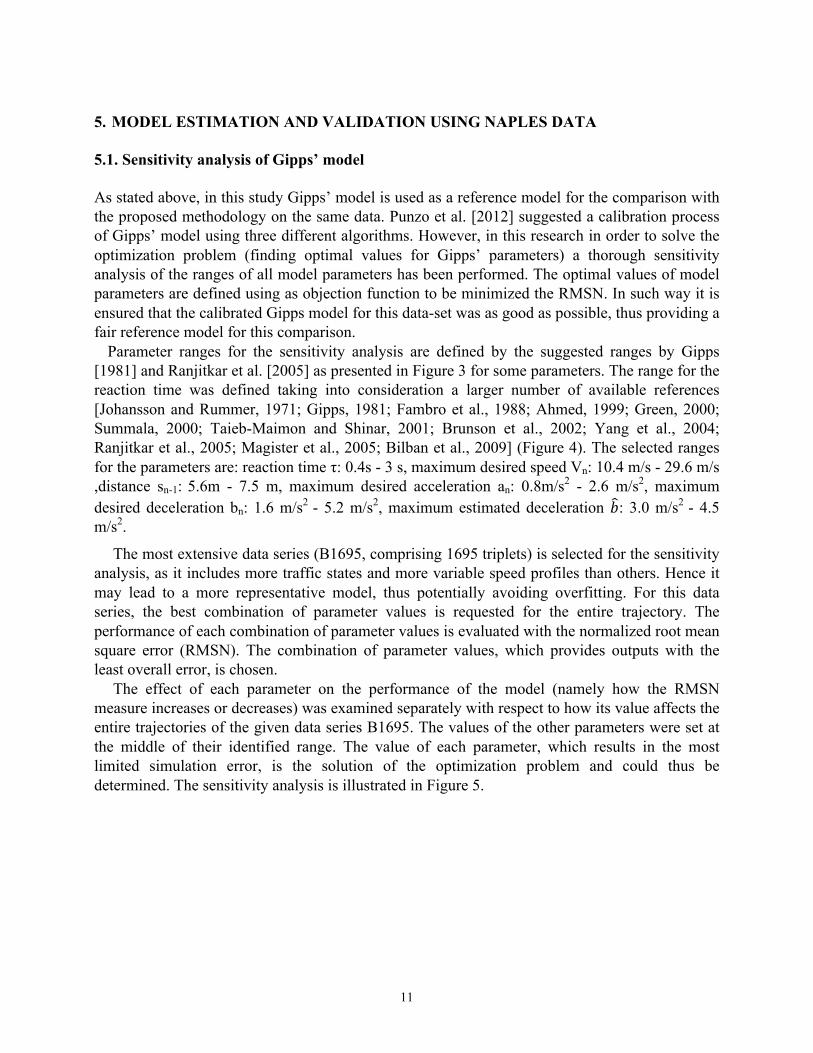
5. MODEL ESTIMATION AND VALIDATION USING NAPLES DATA

5.1. Sensitivity analysis of Gipps’ model

As stated above, in this study Gipps’ model is used as a reference model for the comparison with the proposed methodology on the same data. Punzo et al. [2012] suggested a calibration process of Gipps’ model using three different algorithms. However, in this research in order to solve the optimization problem (finding optimal values for Gipps’ parameters) a thorough sensitivity analysis of the ranges of all model parameters has been performed. The optimal values of model parameters are defined using as objection function to be minimized the RMSN. In such way it is ensured that the calibrated Gipps model for this data-set was as good as possible, thus providing a fair reference model for this comparison.

Parameter ranges for the sensitivity analysis are defined by the suggested ranges by Gipps [1981] and Ranjitkar et al. [2005] as presented in Figure 3 for some parameters. The range for the reaction time was defined taking into consideration a larger number of available references [Johansson and Rummer, 1971; Gipps, 1981; Fambro et al., 1988; Ahmed, 1999; Green, 2000; Summala, 2000; Taieb-Maimon and Shinar, 2001; Brunson et al., 2002; Yang et al., 2004; Ranjitkar et al., 2005; Magister et al., 2005; Bilban et al., 2009] (Figure 4). The selected ranges for the parameters are: reaction time τ: 0.4s - 3 s, maximum desired speed Vn: 10.4 m/s - 29.6 m/s ,distance sn-1: 5.6m - 7.5 m, maximum desired acceleration an: 0.8m/s2 - 2.6 m/s2, maximum desired deceleration bn: 1.6 m/s2 - 5.2 m/s2, maximum estimated deceleration !: 3.0 m/s2 - 4.5 m/s2.

The most extensive data series (B1695, comprising 1695 triplets) is selected for the sensitivity analysis, as it includes more traffic states and more variable speed profiles than others. Hence it may lead to a more representative model, thus potentially avoiding overfitting. For this data series, the best combination of parameter values is requested for the entire trajectory. The performance of each combination of parameter values is evaluated with the normalized root mean square error (RMSN). The combination of parameter values, which provides outputs with the least overall error, is chosen.

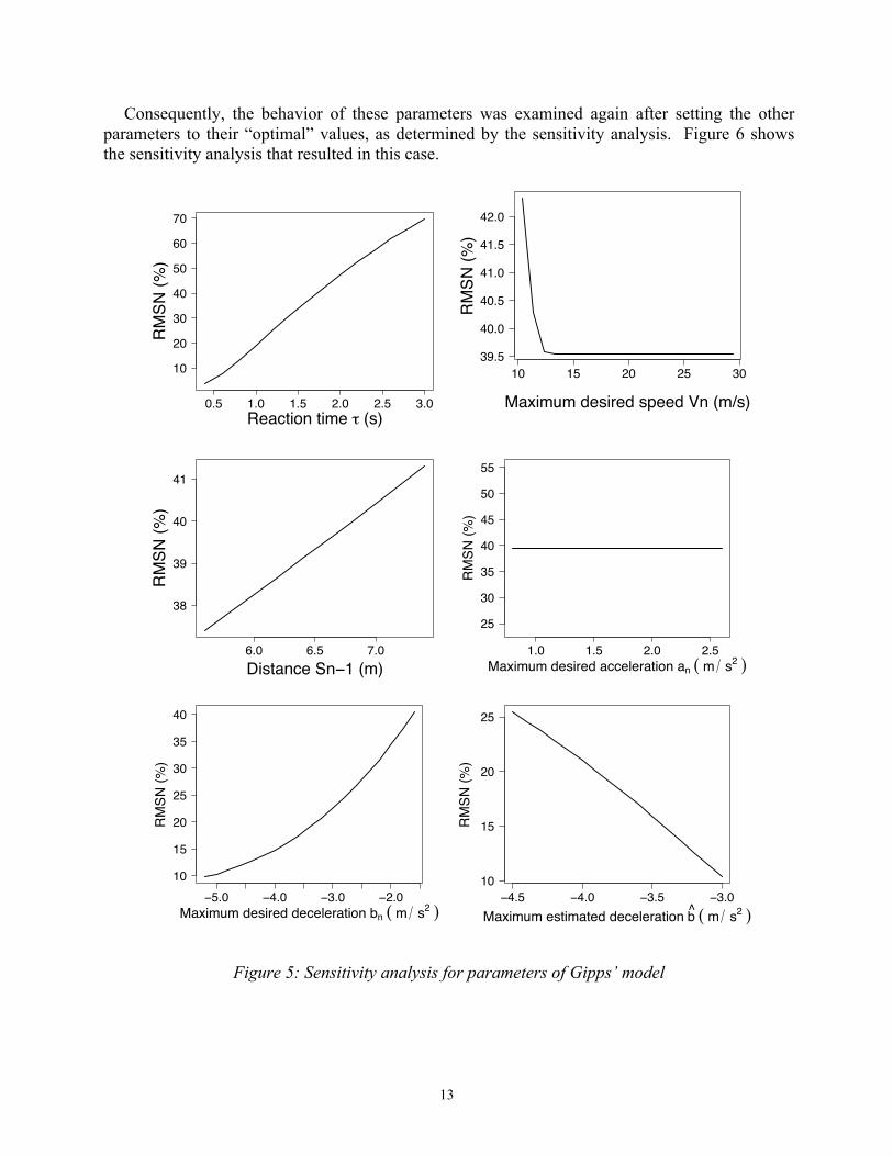
The effect of each parameter on the performance of the model (namely how the RMSN measure increases or decreases) was examined separately with respect to how its value affects the entire trajectories of the given data series B1695. The values of the other parameters were set at the middle of their identified range. The value of each parameter, which results in the most limited simulation error, is the solution of the optimization problem and could thus be determined. The sensitivity analysis is illustrated in Figure 5.

12

Figure 3: Range of Gipps’ parameters according to references

Figure 4: Range for drivers’ reaction time according to references

The influence of speed Vn and maximum acceleration αn is not clear from Figure 5, as some

ranges of these parameters do not seem to affect the RMSN at all. This is due to the observation that both parameters are found only in the first equation of Gipps’ model and for certain parameter values the speed estimation may be provided by the second equation of the model.

Gipps (1981)Ranjitkar et al. (2005)

Selected rangeGipps (1981)

Ranjitkar et al. (2005)Selected range

Gipps (1981)Ranjitkar et al. (2005)

Selected rangeGipps (1981)

Ranjitkar et al. (2005)Selected range

Range of parameters

0 2 4 6 8

Ref

eren

ces

an ( m s2 )

−bn ( m s2 )

− b̂ ( m s2 )

sn−1 ( m s2 )

Johansson and Rummer (1971)

Gipps (1981)Ahmed (1999)

Fabro et al. (1998)Summala (2000)

Taieb−Maimon and Shinar (2001)

Brunson et al. (2002)Ranjitkar et al. (2003)

Green (2000), Yang et al. (2004)

Magister et al. (2005)Ranjitkar et al. (2005)

Bilban et al. (2009)Selected range

Range for reaction time (s)

0.0 0.5 1.0 1.5 2.0 2.5 3.0

Ref

eren

ces

13

Consequently, the behavior of these parameters was examined again after setting the other parameters to their “optimal” values, as determined by the sensitivity analysis. Figure 6 shows the sensitivity analysis that resulted in this case.

Figure 5: Sensitivity analysis for parameters of Gipps’ model

0.5 1.0 1.5 2.0 2.5 3.0

10

20

30

40

50

60

70

Reaction time τ (s)

RM

SN (%

)

10 15 20 25 3039.5

40.0

40.5

41.0

41.5

42.0

Maximum desired speed Vn (m/s)

RM

SN (%

)

6.0 6.5 7.0

38

39

40

41

Distance Sn−1 (m)

RM

SN (%

)

1.0 1.5 2.0 2.5

25

30

35

40

45

50

55

Maximum desired acceleration an ( m s2 )

RM

SN (%

)

−5.0 −4.0 −3.0 −2.010

15

20

25

30

35

40

Maximum desired deceleration bn ( m s2 )

RM

SN (%

)

−4.5 −4.0 −3.5 −3.010

15

20

25

Maximum estimated deceleration b̂ ( m s2 )

RM

SN (%

)

14

Figure 6: Calibration of Gipps’ model

The best performance of Gipps’ model in the calibration data-set was achieved with the following combination of parameters: τ=0.4 s, Vn=14 m/s, αn=0.8 m/s2, sn-1=5.6 m, bn=-5.2 m/s2 and !=-3.0m/s2.

According to Brackstone and McDonald [2003], time steps between 0.1 and 1 second are commonly used in micro-simulation models. Brackstone and McDonald [2003] also suggest that small time steps do not allow for driver error. In addition, Simonelli et al. [2009], applying Gipps’ model using the same data, have also tested values for this apparent reaction time in the range of 0.4-1 sec. Therefore, a second model was also calibrated, in which a value for the reaction time of τ=1.0 s was considered and accordingly a sensitivity analysis was revised. The values of the final parameters are: τ=1.0 s, Vn=16 m/s, αn=1.6 m/s2, sn-1=5.6 m, bn=-5.2 m/s2 and !=-3.0 m/s2. 5.2. Loess application

The models presented in this research were all implemented using the R Software for Statistical Computing [R Development Core Team, 2015]. Application of loess (locally weighted regression) requires the determination of its parameter values, i.e. span (α) and degree (presented in Section 3.2), to ensure a good fit to the data. The span determines how smooth the curve is and it ranges from 0 (wavy curve) to 1 (smooth curve). The degree determines the degree of local polynomials, which are used in each local regression. In the used implementation, a value of 1 refers to a linear function, while 2 in quadratic function. Optimal values of the loess model parameters can be estimated through an optimization approach. A sensitivity analysis was preferred here. The performance of the proposed method for different values of span and degree is presented in Figures 7 and 8 for all available data series in order for appropriate values to be selected. The optimal values are these for which RMSN is minimized.

It is noted that the data that are taken into account for loess are the same with those used in Gipps’ model [speed v2(t) and v3(t) of vehicles 2 and 3 and distance D23(t) between vehicles 2 and 3, as they were estimated by their coordinates], so that a direct and fair comparison between them is possible. It should be mentioned that different combinations of data (v1, v2, v3, v4, D23,

1.0 1.5 2.0 2.5

3.0

3.5

4.0

4.5

5.0

Maximum desired acceleration a (m/s^2)

RM

SN (%

)

10 15 20 25 30

2.8

3.0

3.2

3.4

3.6

Maximum desired speed Vn (m/s)

RM

SN (%

)

15

D34) have also been tested. However, the best performing loess model was this taking into account the same data with Gipps’ model, mainly speed v2(t) and v3(t) and distance D23(t). In addition, for all data series the speed estimation for speed v3(t+τ) with the proposed method relies on the pattern resulting from the entire leader-follower trajectory of data series B1695, as well as the calibration of Gipps’ model. In more detail, the proposed method firstly recognizes the relationships between observations (v2(t) and v3(t) and distance D23(t)) and the response data v3(t+τ) of the B1695 data series. After the relevant pattern from the B1695 data series has been identified, the proposed method is applied to the remainder of the data series. It requires the input data (here speed v2(t) and v3(t) and distance D23(t)) and exports the estimated output v3(t+τ). It should be clarified that reaction time is not a parameter of the loess method. However, it plays a significant role in loess method application, as for different values of reaction time τ different data, mainly data of different time instants, are selected for prediction. For instance, if prediction for time instant t is required, then data for time instant (t-τ) are used. In this research, the same values of reaction time as those used for Gipps’ calibration are used, ensuring a fair comparison..

In Figure 7, the dashed lines illustrate the RMSN of speed v3(t+τ) estimation with proposed method considering degree = 1 for each data series and for each value of span among its range, while the solid lines illustrate the corresponding results for degree = 2.The dashed lines (degree = 1) are smoother and represent lower RMSN than solid lines (degree = 2), and therefore the preferred degree in this case is selected equal to 1. Regarding the span, the dashed lines are almost flat for values of span between 0.4 and 1.0 for all data sets and for both reaction times (0.4s or 1.0s). Consequently, excluding low values, the span does not appear to affect significantly the results. Furthermore, the ranges of the span, for which observed the lowest RMSN for each data series, are presented in Figure 8. The value 0.75 is chosen as average and more representative of the data.

Figure 7: RMSN for different values of span and degree, by applying the method loess for a reaction time τ = 0.4 s

0.2 0.4 0.6 0.8 1.0

2

4

6

8

10

span

RM

SN (%

)

●● ● ● ● ● ● ● ● ● ● ● ● ● ● ● ● ● ●

●

●

●

●●

●● ●

● ● ● ●●

●●

degree=1 degree=2

B1695C621A358A172C168C171

● ●

16

Figure 8: Ranges of span, which minimize the RMSN for each data series

5.3. Validation and results

The accuracy of estimation of the speed v3(t+τ) of the third vehicle was estimated with both

approaches and their performance in terms of RMSN is presented in Figure 9. The loess method provides more reliable results (smaller RMSN errors) for all data sets than Gipps’ model.

Figure 9: Comparison of RMSN by applying Gipps’ model and loess method

Figure 10 presents the same comparison (for reaction time τ=0.4s), but considering more

measures of goodness of fit, used so that both approaches could be evaluated from different points of view, as described in the methodology section. Figure 10 confirms that the proposed

17

method outperforms Gipps’ model. This result confirms the claim that the proposed method comprising locally linear regressions could provide satisfactory results and that data-driven methods could outperform the performance of conventional models.

For reaction time equal to 1s, these measures of goodness of fit were also calculated and it was found that the comparative advantage of the loess method was even larger. Furthermore, we notice that the performance of both models is significantly better for lower values of the reaction time variable t. This could be explained by the fact that a driver with a smaller reaction time could react faster and respond more abruptly to the changes in traffic conditions. Therefore, a model with shorter reaction time would also be able to replicate this driving behavior better.

Figure 10: Comparison of Gipps’ model and loess method for reaction time τ = 0.4 s with

different measures of goodness of fit for the available data series

Besides the aggregate analysis of the model fit, an analysis of the produced residuals is also undertaken, in order to check whether the estimation of speed is biased or not. This could be achieved by testing if the assumptions of normality, linearity and homoscedacity are met or violated. Linearity and homoscedacity could be detected in a plot of residuals versus predicted

B169

5

C621

A358

A172

C168

C171

B169

5

C621

A358

A172

C168

C171

B169

5

C621

A358

A172

C168

C171

0.0

0.1

0.2

0.3

0.4

Gipps’ modelLoess method

RMSN RMSPE MPE

B169

5

C621

A358

A172

C168

C171

B169

5

C621

A358

A172

C168

C171

B169

5

C621

A358

A172

C168

C171

0.0

0.1

0.2

0.3

0.4

0.5

Gipps’ modelLoess method

U Um Us

18

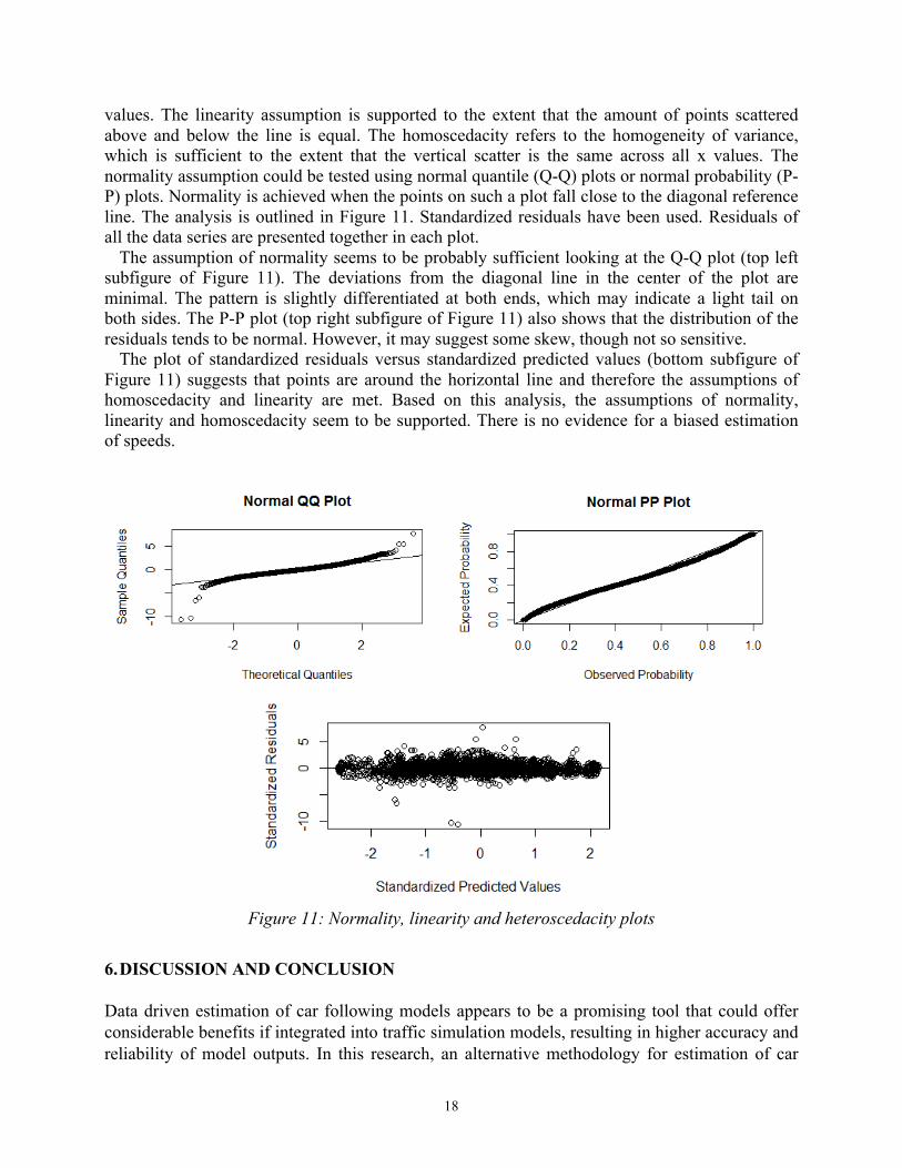
values. The linearity assumption is supported to the extent that the amount of points scattered above and below the line is equal. The homoscedacity refers to the homogeneity of variance, which is sufficient to the extent that the vertical scatter is the same across all x values. The normality assumption could be tested using normal quantile (Q-Q) plots or normal probability (P-P) plots. Normality is achieved when the points on such a plot fall close to the diagonal reference line. The analysis is outlined in Figure 11. Standardized residuals have been used. Residuals of all the data series are presented together in each plot.

The assumption of normality seems to be probably sufficient looking at the Q-Q plot (top left subfigure of Figure 11). The deviations from the diagonal line in the center of the plot are minimal. The pattern is slightly differentiated at both ends, which may indicate a light tail on both sides. The P-P plot (top right subfigure of Figure 11) also shows that the distribution of the residuals tends to be normal. However, it may suggest some skew, though not so sensitive.

The plot of standardized residuals versus standardized predicted values (bottom subfigure of Figure 11) suggests that points are around the horizontal line and therefore the assumptions of homoscedacity and linearity are met. Based on this analysis, the assumptions of normality, linearity and homoscedacity seem to be supported. There is no evidence for a biased estimation of speeds.

Figure 11: Normality, linearity and heteroscedacity plots

6. DISCUSSION AND CONCLUSION Data driven estimation of car following models appears to be a promising tool that could offer considerable benefits if integrated into traffic simulation models, resulting in higher accuracy and reliability of model outputs. In this research, an alternative methodology for estimation of car

19

following models has been presented. A simulation optimization of car-following models could be achieved using the proposed method. The proposed method outperforms the reference (Gipps’) model for all available data. This research corroborates results from other studies (Simonelli et al. [2009]; Bifulco et al. [2013]), which imply that data-driven methods could provide better estimation than conventional models. The additional contribution of this work is to suggest an easy and quick methodology for estimation of car-following models, especially for applications that individual and personalized models are not so critically necessary.

Machine learning methods present great flexibility and speed in managing data, avoiding the time consuming process of parameter calibration, which is essential for traditional car following models. The most important advantage of the proposed method is that it does not require the specification of a function to fit a model simultaneously to all the data in a sample. There is only the need to define the smoothing parameter and the degree of the local polynomial, avoiding time-consuming calculations for traffic model calibration. Moreover, the loess method could be helpful and flexible in specific and complex traffic situations (for instance emergency cases), for which no theoretical models may exist or it is complicated to be specified. Therefore the proposed method can be used in calibration issues, where computational ability of classical methods is limited. Furthermore, it provides the opportunity for incorporation of additional parameters without the need to resort to cumbersome reformulations of the model functional form. The loess procedure is suitable for data with outliers (not extreme), when a robust fitting method is essential. On the other hand, the loess method cannot be represented by a mathematical formula and it is thus difficult to transfer the results to other cases. It should be also referred that too large data series may require too much memory for loess application and that extreme outliers may overcome the method.

While this research focused on the longitudinal interaction among vehicles moving in sequence, there are many other perspectives of the issue that have not been considered, such as the lateral interaction of a vehicle with vehicles in near-by lanes, as well as interactions between vehicles and road infrastructure (road curvature, existence of stop or traffic light at intersections, etc.). However, it is noted that Brackstone et al. [2009] detected little correlation between road type and driving behavior. Other factors, which could influence driving behavior and may be incorporated into the process, include drivers’ characteristics, such as age, reaction time and experience. Moreover, heterogeneity of data could be addressed by more specific car-following models moving towards clustered models. This could be an interesting topic for future work.

This paper suggests that data-driven methods could provide reliable results and potentially more accurate than traditional car following models. However, traditional car-following models have the advantage of basing their output on traffic flow theory. In contrast, despite their flexibility, computational approaches do not contribute as much in the advancement of traffic flow theory, may not be necessarily comprehensible by the human mind.

Integration of data-driven methods in the simulation process requires additional studies that will further confirm their validity. Technological advancements will contribute significantly into the collection of data, which could in turn result to more robust and reliable models. Although many theoretical models have been developed so far, there is lack of a robust model that could generally represent car-following behaviors under all conditions. Data driven methods can be a plausible substitute for theory-based models and this research provides a contribution towards this direction. Naturally, a lot of further research is needed to elucidate further aspects of its

20

applications and verify its robustness. ACKNOWLEDGMENTS Research supported by the Action: ARISTEIA-II (Action’s Beneficiary: General Secretariat for Research and Technology), co-financed by the European Union (European Social Fund – ESF) and Greek national funds. The authors would like to thank Prof. Vincenzo Punzo from the University of Napoli–Federico II for kindly providing the data used in this research.

REFERENCES

Ahmed K. I. (1999). Modeling Drivers’ Acceleration and Lane Changing Behavior, PhD thesis, Massachusetts Institute of Technology, Cambridge, Mass., 1999.

Al-Shihabi, T. and Mourant, R.R. (2003). Toward More Realistic Driving Behavior Models for Autonomous Vehicles in Driving Simulators. 82nd Annual Meeting of the Transportation Research Board, Washington, D. C. Antoniou C. and H. N. Koutsopoulos (2006). Estimation of Traffic Dynamics Models with Machine Learning Methods. Transportation Research Record: Journal of the Transportation Research Board, No. 1965, pp. 103-111, Washington D.C., 2006.

Antoniou, C., R. Balakrishna and H. N. Koutsopoulos (2011). A synthesis of emerging data collection technologies and their impact on traffic management applications. European Transport Research Review, Volume 3, Number 3, 139-148, DOI: 10.1007/s12544-011-0058-1. Antoniou C., H.N. Koutsopoulos and G. Yannis (2013). Dynamic Data-Driven Local Traffic State Estimation and Prediction, Transportation Research - Part C: Emerging technologies, Vol. 34, pp. 89-107.

Antoniou, C., V. Gikas, V. Papathanasopoulou, T. Mpimis, I. Markou and H. Perakis (2014). Towards distribution-based calibration for traffic simulation. 17th International IEEE Conference on Intelligent Transportation Systems, Qingdao, China, October 8-11, pp. 780-785. Atkenson, C. G., A. Moore, and S. Schaal. Locally Weighted Learning. AI Review, Vol. 11, 1997, pp. 11–73. Aycin, M. F., and Benekohal, R. F. (1999). Comparison of car-following models for simulation. Transportation Research Record: Journal of the Transportation Research Board, 1678(1), 116-127.

Aw, A., Klar, A., Rascle, M., & Materne, T. (2002). Derivation of continuum traffic flow models from microscopic follow-the-leader models. SIAM Journal on Applied Mathematics, 63(1), 259-278. Bando, M., K. Hasebe, A. Nakayama, A. Shibata, and Y. Sugiyama (1995). Dynamical model of traffic congestion and numerical simulation. Physical Review E, 51(2): 1035-1042. Bando, M., K. Hasebe, K. Nakanishi, and A. Nakayama (1998). Analysis of optimal velocity model with explicit delay. Physical Review E, 58(5): 5429-5435.

21

Barceló, J. (2002). Dynamic Network Simulation with AIMSUN. Proc., International Symposium on Transport Simulation, Yokohama, Aug. Kluwer Academic Publishers. Barceló, J. (ed.) (2010). Fundamentals of Traffic Simulation, volume 145 of International Series in Operations Research & Management Science, Springer. Bellemans T., De Schutter B. and De Moor B. (2002). “Models for traffic control”, Journal A., Vol 43, no 3-4, pp. 13-22. Bierley, R.L., 1963. Investigation of an inter vehicle spacing display. Highway Research Record 25, 58–75. Bifulco G.N., L. Pariota, F. Simonelli, R. Di Pace (2013). Development and testing of a fully Adaptive Cruise Control system. Transportation Research Part C, 29 (2013), pp. 156–170. Bilban M., Alenka Vojvoda and Janez Jerman (2009). Age Affects Drivers’ Response Times, Coll. Antropol. 33 (2009) 2: 467–471. Boxill S.A. and L. Yu (2000). An Evaluation of Traffic Simulation Models for Supporting ITS Development. Center for Transportation Training and Research Texas Southern University. Brackstone, M., McDonald, M., 1999. Car-following: a historical review. Transportation Research Part F 2 (4), 181–196 Brackstone, M. and McDonald, M., (2003). Driver Behaviour and Traffic Modelling: Are we looking at the Right Issues? Transportation Research Group, Dept. of Civil and Environmental Engineering, University of Southampton, U.K.

Brackstone M, Waterson B & McDonald M (2009) “Determinants of Following Headway in Congested Traffic”, Transportation Research Part F: Traffic Psychology and Behavior, 12(2), p131-142. Brunson S. J., E. M. Kyle, N.C. Phamdo and G. R. Preziotti (2002). Alert algorithm development program: NHTSA rear-end collision alert algorithm. DOT HS 809-526, Final Report, The John Hopkins University in cooperation with the NHTSA and General Motors Corporation.

Chakroborty, P., & Kikuchi, S. (1999). Evaluation of the General Motors based car-following models and a proposed fuzzy inference model. Transportation Research Part C: Emerging Technologies, 7(4), 209-235. Chandler, R.E., Herman, R., Montroll, E.W., 1958. Traffic dynamics: studies in car following. Operations Research 6 (2), 165–184. Chong, L., Abbas, M. M., Medina Flintsch, A., & Higgs, B. (2013). A rule-based neural network approach to model driver naturalistic behavior in traffic. Transportation Research Part C: Emerging Technologies, 32, 207-223.

Ciuffo B., Punzo V. and Montanino M. 2012. 30 years of the Gipps’ car-following model: applications, developments and new features. Transportation Research Record 2315, p. 89-99.

Cleveland W. S. (1979). Robust Locally Weighted Regression and Smoothing Scatterplots, Journal of the American Statistical Association, Vol. 74, 1978, pp. 829–836.

22

Cleveland W. S., and S. J. Devlin (1988). Locally Weighted Regression: An Approach to Regression Analysis by Local Fitting, Journal of the American Statistical Association, Vol. 83, 1988, pp. 596–610.

Cleveland, W. S., S. J. Devlin, and E. Grosse (1988). Regression by Local Fitting: Methods, Properties and Computational Algorithms. Journal of Econometrics, Vol. 37, 1988, pp. 87–114.

Cleveland W. S., Eric Grosse, and Ming-Jen Shyu (1996). A Package of C and Fortran Routines for Fitting Local Regression Models: Loess User's Manual, Bell Labs, Technical Report.

Cohen, R. A. (1999), "An Introduction to PROC LOESS for Local Regression," Proceedings of the 24th SAS Users Group International Conference, Paper 273.

Colombaroni C., G Fusco (2013). Artificial Neural Network Models for car following: experimental analysis and calibration issues- Journal of Intelligent Transportation Systems, Volume 18, Issue 1, 2014. Davis, L. C. (2003). Modifications of the optimal velocity traffic model to include delay due to driver reaction time. Physica A: Statistical Mechanics and its Applications, 319, 557-567. Dunne, S. and B. Ghosh (2012). Regime-based short-term multivariate traffic condition forecasting algorithm. Journal of Transportation Engineering, Vol. 138, No. 4, pp. 455-466. Edie, L.C., 1961. Car-Following and Steady-State Theory for Non-congested Traffic. Operations Research 9 (1), 66–76, http://dx.doi.org/10.2307/167431. Elhenawy, M., Chen, H., & Rakha, H. A. (2014). Dynamic travel time prediction using data clustering and genetic programming. Transportation Research Part C: Emerging Technologies, 42, 82-98.

Fambro D. B., R. J. Koppa, D. L. Picha, and K. Fitzpatrick (1988). Driver Perception- Brake Response in Stopping Sight Distance Situations. In Transportation Research Record 1628, TRB, National Research Council, Washington. D.C., 1998, pp. 1–7. Fritzsche, H.T. (1994). A Model for Traffic Simulation. Traffic Engineering and Control, May, 317-321. Gazis, D.C., Herman, R., Rothery, R.W., 1961. Nonlinear follow-the-leader models of traffic flow. Operations Research 9 (4), 545–567, <http://www.jstor.org/stable/167126>. Gipps P.G. (1981). A Behavioral Car Following Model for Computer Simulation. Transportation Research B 15, pp. 105-111. Green M. (2000). “How Long Does It Take to Stop?” Methodological Analysis of Driver Perception-Brake Times.” Transportation Human Factors, vol. 2, no. 3, pp.195–216, 2000. Greenberg H. An Analysis of Traffic Flow. Operations Research, Vol. 7, 1959, pp. 79–85.

Hamdar S. H. & Mahmassani H. S. (2008). Driver car-following behavior: From discrete event process to continuous set of episodes. Transportation Research Board Annual Meeting.

Helbing, D., B. Tilch, Phys. Rev. E 58 (1998) 133–138. Helly, W., 1961. Simulation of bottlenecks in single lane traffic flow. In: Theory of Traffic Flow. Elsevier Publishing Co., pp. 207–238.

23

Herman, R., Montroll, E.W., Potts, R.B., Rothery, R.W., 1959. Traffic dynamics: analysis of stability in car following. Operations Research 7 (1), 86–106, <http://www.jstor.org/stable/167596>.

Herman, R., Rothery, R.W., 1965. Car following and steady-state flow. In: Proceedings of the 2nd International Symposium on the Theory of Traffic Flow, pp.1–11.

Hidas P. (1998). A car-following model for urban traffic simulation. Traffic Engineering and Control, 39, pp. 300-305.

Huang E., Antoniou C., Wen Y., Ben-Akiva M., Lopes J., Bento J. (2009). “Real-time multi-sensor multi-source network data fusion using dynamic traffic assignment models.” Intelligent Transportation Systems, 2009, ITSC '09, 12th International IEEE Conference on, 2009, 1-6. Jiang, R., Q.S. Wu, Z.J. Zhu (2001). Full velocity difference model for a car-following theory. Phys. Rev. E 64, 017101. Johansson G., and K. Rummer (1971). Drivers’ Brake Reaction Time. Human Factors, Vol. 13, No. 1, 1971, p. 23. Karlaftis, M.G., E.I. Vlahogianni (2011). Statistical methods versus neural networks in transportation research: Differences, similarities and some insights, Transportation Research Part C: Emerging Technologies, Volume 19, Issue 3, June 2011, Pages 387-399, ISSN 0968-090X, http://dx.doi.org/10.1016/j.trc.2010.10.004.

Kikuchi, C. and Chakroborty, P. (1992). Car following model based on a fuzzy inference system. Transportation Research Record, 1365, 82-91.

Kometani, E., Sasaki, T., 1958. On the stability of traffic flow. Report no. 1. Journal of Operations Research Japan 2 (1), 11–26.

Koutsopoulos N. H. and H. Farah (2012). Latent class model for car following behavior, Transportation Research Part B 46 (2012) 563–578.

Lenz, H., Wagner, C.K., Sollacher, R., 1999. Multi-anticipative car-following model. The European Physical Journal B 7 (2), 331–335

Leutzbach, W., 1988. Introduction to the Theory of Traffic Flow. Springer Verlag, Berlin. Liu R. (2010). Traffic simulation with DRACULA. Fundamentals of Traffic Simulation (Ed. J Barceló), Springer. Olstam J., J. Tapani A. (2004). Comparison of Car-following models. Swedish National Road and Transport Research Institute,VTI meddelande 960A · 2004. Orosz, G., Krauskopf, B., and Wilson, R. E. (2005). Bifurcations and multiple traffic jams in a car-following model with reaction-time delay. Physica D: Nonlinear Phenomena, 211(3), 277-293.

Pindyck R.S., and D.L. Rubinfeld (1997). Econometric Models and Economic Forecasts, 4th ed. Irwin McGraw-Hill. Boston, Mass., 1977.

Pipes, L.A., 1953. An operational analysis of traffic dynamics. Journal of Applied Physics 24 (3), 274–281.

24

Pipes, L.A., 1967. Car-following models and the fundamental diagram of road traffic. Transportation Research 1 (1), 21–29. Punzo, V., Formisano, D. J., & Torrieri, V. (2005). Part 1: Traffic flow theory and car following: Nonstationary kalman filter for estimation of accurate and consistent car-following data. Transportation Research Record: Journal of the Transportation Research Board, 1934(1), 1-12.

Punzo, V., Borzacchiello, M. T., & Ciuffo, B. (2011). On the assessment of vehicle trajectory data accuracy and application to the Next Generation SIMulation (NGSIM) program data. Transportation Research Part C: Emerging Technologies, 19(6), 1243-1262.

Punzo V., Ciuffo B., and Montanino. M (2012). May we trust results of car following models calibration based on trajectory data? In Proceedings of the 91st Annual Meeting of the Transportation Research Board, Washington, D.C. R Development Core Team (2015). R: A Language and Environment for Statistical Computing. R Foundation for Statistical Computing, Vienna, Austria. www.R-project.org. Accessed January 20, 2015.

Rakha H., Wang W. (2009). Procedure for calibrating Gipps car-following model. Transportation Research Record, 2124, pp. 113-124.

Ranjitkar P., Suzuki H. and Nakatsuji T. (2005). Microscopic traffic data with real-time kinematic global positioning system. Proceedings of Annual Meeting of Infrastructure Planning and Management, Japan Society of Civil Engineer, Miyazaki, Preprint CD, December, 2005. Reuschel, R., 1950. Fahrzeugbewegungen in der Kolonne. Osterreichisches Ingenieur Archiv 4, 193–215. Sawada, S. (2002). Generalized optimal velocity model for traffic flow. International Journal of Modern Physics C, 13(01), 1-12. Silcock. J.P. (1993). SIGSIM version 1.0 users guide. Working Paper, Centre for Transport Studies, University of London. Simonelli, F., Bifulco, G. N., De Martinis, V., and Punzo, V. (2009). Human-like adaptive cruise control systems through a learning machine approach. In Applications of Soft Computing (pp. 240-249). Springer Berlin Heidelberg.

Spyropoulou, I., “Gipps car following model - an in-depth analysis”, Transportmetrica, 3(3), 231-245, 2007.

Subramanian, H. (1996). Estimation of car-following models (Doctoral dissertation, Massachusetts Institute of Technology).

Summala H. (2000). Brake reaction times and driver behavior analysis. Transportation Human Factors, 2(3), pp. 217-226.

Taieb-Maimon M. and D. Shinar (2001). Minimum and comfortable driving headways: reality versus perception. Human Factors, Vol. 43, No. 1, pp. 159-172.

Theil H. (1978). Introduction to Econometrics, Prentice Hall, New Jersey.

25

Treiber, M., Hennecke, A., & Helbing, D. (2000). Congested traffic states in empirical observations and microscopic simulations. Physical Review E, 62(2), 1805 Toledo T. (2003). Integrated Driving Behaviour Modelling. PhD thesis, Massachusetts Institute of Technology. Tordeux, A., Lassarre, S., Roussignol, M., (2010). An adaptive time gap car-following model. Transportation Research Part B 44 (8–9), 1115–1131. Treiber, M., Kesting, A., Helbing, D., (2006). Delays, inaccuracies and anticipation in microscopic traffic models. Physics A 360 (1), 71–88. Underwood, R.T., 1961. Speed volume and density relationships: quality and theory of traffic flow. Bureau of Highway Traffic, Yale University, 141–188. US Department of Transportation (2012). “NGSIM – Next Generation Simulation.” http://www.ngsim.fhwa.dot.gov van Lint, J.W.C. (2005). Accurate freeway travel time prediction with state-space neural networks under missing data. Transportation Research Part C: Emerging Technologies, Vol. 13, pp. 347-369.

van Lint, J.W.C. (2008). Online Learning Solutions for Freeway Travel Time Prediction. IEEE Transactions on Intelligent Transportation Systems. Vol. 9, Iss. 1, pp. 38-47.

Vlahogianni, E. I., M. G. Karlaftis, and J. C. Golias (2005). Optimized and meta-optimized neural networks for short-term traffic flow prediction: A genetic approach. Transportation Research C. 13 (3), pp. 211-234. Vlahogianni, E.I., M.G. Karlaftis and J. C. Golias (2008). Temporal evolution of short-term urban traffic flow: A nonlinear dynamics approach. Computer-Aided Civil and Infrastructure Engineering 23, pp. 536–548.

Wang. L., J. Rong and X. Liu (2005). The Classification of Car-Following Behavior in Urban Expressway Based on Fuzzy Clustering Analysis. Proceedings of the 84th Annual Meeting of the Transportation Research Board, Washington, D.C. Wiedemann, R., 1974. Simulation des Straenverkehrsflusses. Schriftenreihe des Instituts fuer Verkehrswesen, Universitaet Karlsruhe, Heft 8. Wiedemann, R., Reiter, U., 1992. Microscopic traffic simulation: the simulation system MISSION, background and actual state. CEC Project ICARUS (V1052), Final Report, vol. 2. CEC, Brussels (Appendix A).

Wilson R.E. (2000). An analysis of Gipps’ car-following model of highway traffic. IMA Journal of Applied Mathematics, 66, pp. 509-537.

Yang, Q., Koutsopoulos, H.N., 1996. A microscopic traffic simulator for evaluation of dynamic traffic management systems. Transportation Research Part C 4 (3), 113–129.

Yang, X., Liu, J., Vaidya, N. F., & Zhao, F. (2004). A vehicle-to-vehicle communication protocol for cooperative collision warning. In Mobile and Ubiquitous Systems: Networking and Services, 2004. MOBIQUITOUS 2004. The First Annual International Conference on (pp. 114-123). IEEE. Zhang, H.M. and T. Kim (2005). A car-following theory for multiphase vehicular traffic flow. Transportation Research Part B 39, 385–399.

26

Zhang, J. F-Y Wang, K. Wang, W-H Lin, X. Xu, C. Chen (2011). "Data Driven Intelligent Transportation Systems: A Survey," IEEE Transactions on Intelligent Transportation Systems, vol. 12, 4, pp. 1624- 1639,.

Zhao, X., & Gao, Z. (2005). A new car-following model: full velocity and acceleration difference model. The European Physical Journal B-Condensed Matter and Complex Systems, 47(1), 145-150. Zheng, J., Suzuki, K., & Fujita, M. (2013). Car-following behavior with instantaneous driver–vehicle reaction delay: A neural-network-based methodology. Transportation Research Part C: Emerging Technologies, 36, 339-351.