variability of sea state measurements and sensor dependence · the sea floor at the ekofisk field...

Utskifting av

bakgrunnsbilde:

- Høyreklikk på

lysbildet og velg

«Formater

bakgrunn»

- Under «Fyll», velg

«Bilde eller tekstur»

og deretter «Fil…»

- Velg ønsket

bakgrunnsbilde og

klikk «Åpne»

- Avslutt med å velge

«Lukk»

Variability of sea state measurements

and sensor dependence Anne Karin Magnusson

MET-Norway, Bergen

R&D, Operational Oceanography and Marine Meteorology

Workshop: Statistical models of the Metocean environment for engineering uses

IFREMER 30.09-01.10.2013

Utskifting av

bakgrunnsbilde:

- Høyreklikk på

lysbildet og velg

«Formater

bakgrunn»

- Under «Fyll», velg

«Bilde eller tekstur»

og deretter «Fil…»

- Velg ønsket

bakgrunnsbilde og

klikk «Åpne»

- Avslutt med å velge

«Lukk»

CONTENT

- Background

- The Ekofisk wave sensors

• Searching for «a true sea state»

• Intrisic variability

• location effects

- A long swell case in central North Sea

EKOFISK, 56.5 N 3.2 E

The sea floor at the Ekofisk field

is subsiding due to the oil extraction,

and constructions are therefor more and

more exposed to wave forces.

«EXWW» are special procedures

developed between Phillips Petroleum -

now ConocoPhillips - and MET-Norway to

ensure safe activity offshore.

In this, monitoring of environmental

parameters in real time is of primary

importance.

EKOFISK and EXWW

(Ekofisk eXtreme Wave Warning)

met.no: EEkofisk extreme wave forecasting OCEANOBS’04

Waverider

Laser Flare South

Laser Flare North

Environmental parameters: Atmospheric pressure, air and sea temperature, wind from 2 sensors. Current

Wave data from 4 wave recorders. Since 2003: also from LASAR (4 lasers in array)

WAMOS (marine radar)

LASAR

Ekofisk: from 1986 until «today»

6

Norwegian Meteorological Institute

Motivation for study on variability in wave data

· A ”true sea state” is needed for - VALIDATION of wave forecasting models

hindcast and forecast - In real time, for performance of marine operations

· This ”True sea state” is difficult to assess – from many

reasons: - Intrisic variability - 20 minutes the shorter timeseries - the higher the

variability - Location (lee effects, sea spray … - Sensor type (what is measured?)

Experience from forecasting and monitoring:

Some large differences are seen in Hs (as much as 20%) between the different sensors

Also a problem: Hs has very high variability within 20 minutes measurements. we should evaluate wave parameters over 30 minutes!


MRF (2Hz):

MIROS Range Finder

(Altimeter)

LASAR (5 Hz) : 4 lasers in a square

array (2.6x2.6m)

N

2/4-H

Ekofisk 56.5N 3.2E operated by ConocoPhillips

K ----- B

K

Datawell

Waverider

Heave buoy

(2Hz)

1 2 3

4

Norwegian Meteorological Institute 9

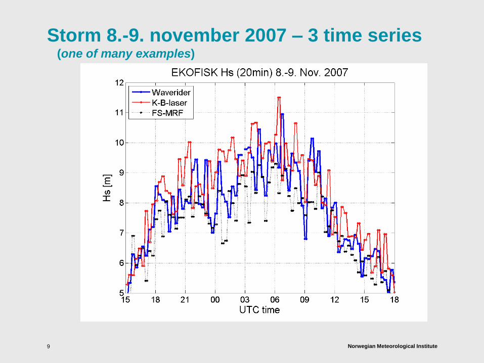
Storm 8.-9. november 2007 – 3 time series (one of many examples)


20-min Hs values

Hs max 20min= 11 m Waverider


HOURLY HS values

Hs max 1-hrly= 10 m Waverider


2-hourly Hs values

Hs max 2-hrly= 9.5m Waverider


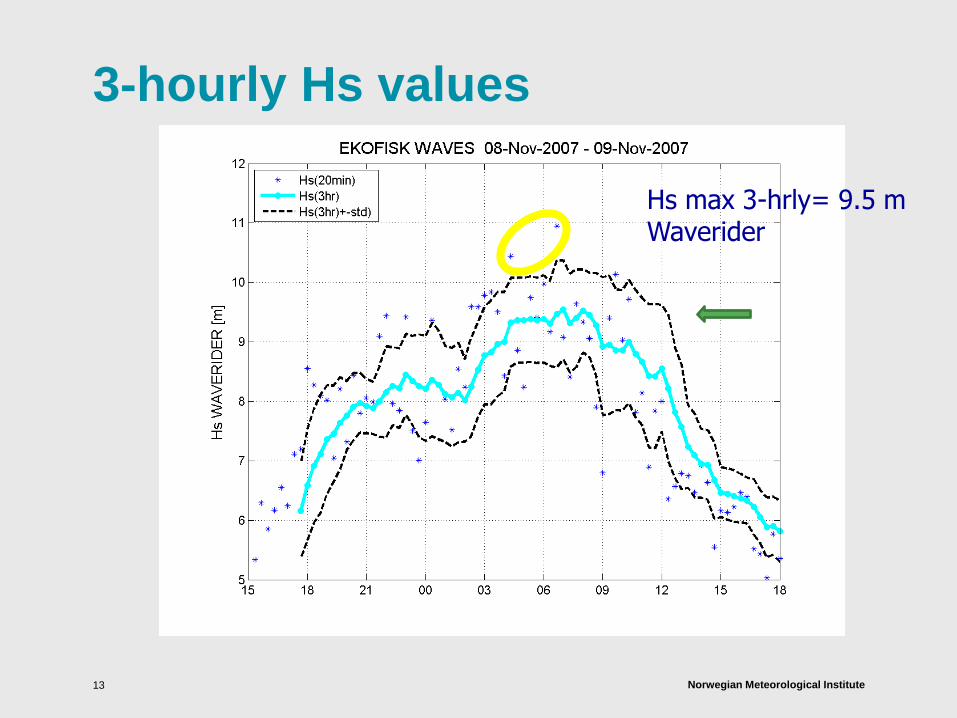
3-hourly Hs values

Hs max 3-hrly= 9.5 m Waverider


Questions to answer

10.10.2013

What causes differences?

- Lee effects of constructions

- Sea spray intensifying?

- Quality assurance that filters high crests?

- Inherent sensor discreepancies?

- Natural variability in sea state

14


DATA : 20 STORMS CASES FROM 2007 and 2008

(From 11th Wave Workshop, Halifax, 2009, and 12th, Hawaii, Nov. 2011


Comparison of Hs in 20 storms jan2007-dec2008

LASAR vs Waverider Miros MRF vs Waverider

Hs : 0 - 12 m

Hs

: 0 -

12 m

H

s :

0 -

12 m

Hs : 0 - 12 m


Hs comparison (sensors and time averaging)

1hrly 1hrly

Hourly averages

have higher

correlations

HsLASAR= 0.99.HsWR+ 0.28

Corr=0.95 (1-hourly)

Hs = 5 m : 5 % lower

Hs = 10 m : 10 % lower

HsMRF = 0.86 *HsWR + 0.5

Corr = 0.93 (1-hourly)

20min 20min


Comparison of Hs in 20 storms jan2007-oct2009

qq-plot

LASAR

MRF

Waverider Waverider

Axes: 2-12m


Average Hs in Wind dir sectors (dθ=10°)

230-250: Sea spray on LASAR?

180 210 240 270 300 330 360 030


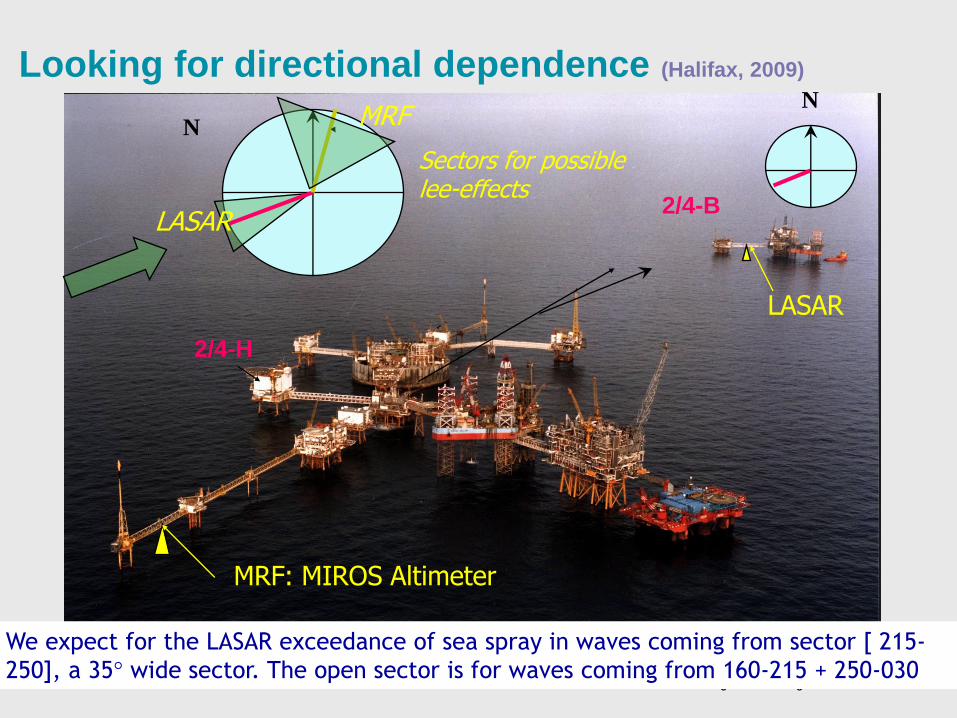
Looking for directional dependence (Halifax, 2009)

MRF: MIROS Altimeter

LASAR

N

N

2/4-B

2/4-H

Sectors for possible lee-effects

MRF

LASAR

We expect for the LASAR exceedance of sea spray in waves coming from sector [ 215-

250], a 35° wide sector. The open sector is for waves coming from 160-215 + 250-030


Searching for a common open (’exposed’) sector

The sea spray sector

[-5 % - +10 %]

In ’open sector’ the MRF

has slightly lower <Hs> (3-6%)

Still mostly negativ.

More pronounced lee effects for dd>300

[shift of +3 %]

180 210 240 270 300 330 360 030


The ’open sector’ is not always what it appears to be

18UTC: Mean wind and wave directions are OK (in

open sector), but we see relatively large amounts of

wave energi from North (waves at MRF are then partly

going through the other platforms )

12utc

00utc 18utc

15utc Wind dir

Wind speed

Hs

Tp

20m/s

10m


Wind and wave field in

the Andrea storm, when

a freak wave was

measured.

Wind speed at 00 UTC

Hs at 03 UTC

We see an area with

different wave peak direction

is moving southward

towards Ekofisk


Hypothesis regarding the differences

· Not all differences are due to local effects (sheltering, too much sea spray…)

· Some are due to too strict quality control on raw data - Limiting steepness?

Not only spray like here, giving f.ex spikes

But possibly also limiting values of steepness


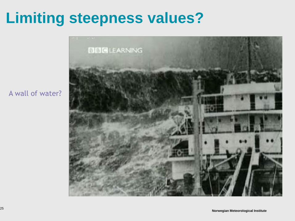
Limiting steepness values?

A wall of water?


Conclusions

· Different measuring techniques give

different wave statistics. (this is

common knowledge?)

· The question is if it is because of

sheltering effects only!?

· Waverider data, although unskewed,

give good Hs up to 9m


Other work on sensor dependences

WACSIS: Wave Crest Sensor Intercomparison Study

· A Joint Industry Project (JIP) by SHELL Global Solutions U.S. and IFREMER

· Dec 1997-may 1998: a set of wave sensors were mounted on the Dutch

Meetpost Noordwijk measurement platform ( on coast of the Netherlands)

- Baylor wave staff

- THORN wave height sensor (an upgrade of the EMI laser)

- MAREX SO5 wave radar

- Vlissingen step gauge and Marine 300 step gauge

- directional waverider buoy

- SMART 800 GPS buoy

- WAVEC directional buoy

- S4ADW current meter and pressure sensor

· Report, January 2001: Marc Prevosto, George Z. Forristall, Sylvie Van Iseghem,

Benjamin Moreau

Uncertainty due to sampling

variability

· Statistical uncertainty (sampling variability) is due to a limited number

of observations of a quantity, regions or time periods when data are

missing, and other sampling biases.

· Donelan and Pierson (1983) investigated both laboratory and field data

showed 8% variability for Hs.

· Bitner-Gregersen and Hagen (1990) analysed theoretically this

variability for both wave heights and periods.

REFERENCES: • Bitner-Gregersen, E. M. and Hagen, Ø., 1990: Uncertainties in Data for the Offshore

Environment, Structural Safety, 7, 11–34, doi:10.1016/0167-4730(90)90010-M, 1990.

• Donelan, M.A., and W.J. Pierson, 1983: The Sampling Variability of Estimates of Spectra of

Wind Generated Gravity Waves. Journal of Geophysical Research, Vol. 88, No. C7, pp.

4381-4392, May, 1983

10.10.2013 28

Variability

• Bitner-Gregersen, E. M. and Hagen, Ø., 1990: Uncertainties in Data for the

Offshore Environment, Structural Safety, 7, 11–34, doi:10.1016/0167-

4730(90)90010-M, 1990.

· The sampling variability in standard deviation (in %) of Hm0 for the

Jonswap spectrum.

10.10.2013 Bunntekst 29

Sampling variability standard

deviation sig_HM0 (in %) of HM0 for

the Jonswap spectrum

10.10.2013 30

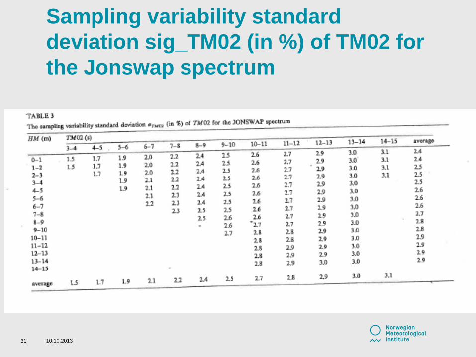
Sampling variability standard

deviation sig_TM02 (in %) of TM02 for

the Jonswap spectrum

10.10.2013 31

Norwegian Meteorological Institute 10.10.2013 Bunntekst 32

Approach to validate the theoretical values with data:

(Source: EGU poster, Bitner-Gregersen and Magnusson, EGU 2013):

• Continuous measurements of wave profile at 2Hz sampling rate are gathered in 60minutes

time series.

• 22 consecutive windows of 17.5 minutes length, with increament of 2 min over each 60

minutes records, are used to evaluate sampling variability of Hs and Tz.


24 ’hourly values’ of Hs - per day

Within each hour: (17.5:2.5:60min) =

17 possible ’catches’ of Hs_{17.5min}

Ongoing work on variability in Hs estimates


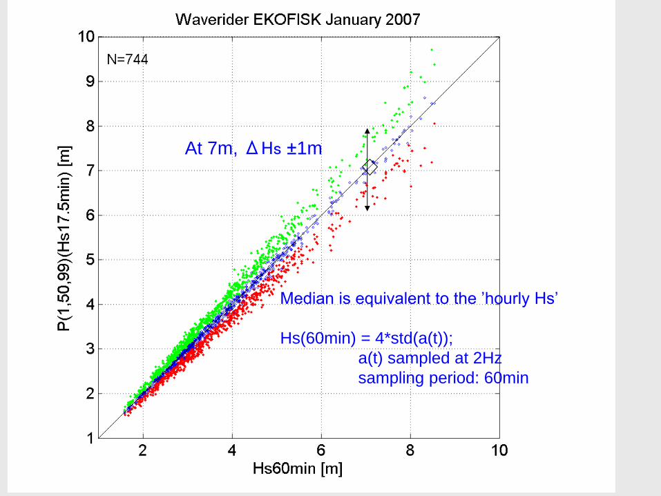
Median is equivalent to the ’hourly Hs’

Hs(60min) = 4*std(a(t));

a(t) sampled at 2Hz

sampling period: 60min

At 7m, ΔHs ±1m


One day of data comparing Hs and Tz over different sampling periods

10.10.2013 35

SIGNIFICANT WAVE HEIGHT WAVE MEAN PERIOD


Standard deviation in % of the 17.5

minute values of wave height or period

as function of the 60 minutes values.

36

The standard deviations are seen to be very variable, The spread is

though higher for Hs than for TZ (TM02), showing similarity with

numbers given in the tables from Bitner-Gregersen and Hagen, 1990. (ongoing work)

(5.5-5.6%) (2.5-2.6%)

Swell cases in the North Sea

· Example of data that could be used in PhD?

10.10.2013 Bunntekst 37


A long swell case at Ekofisk

10.10.2013 38


Swell arriving at Ekofisk

around 23UTC 20th august 2013

39


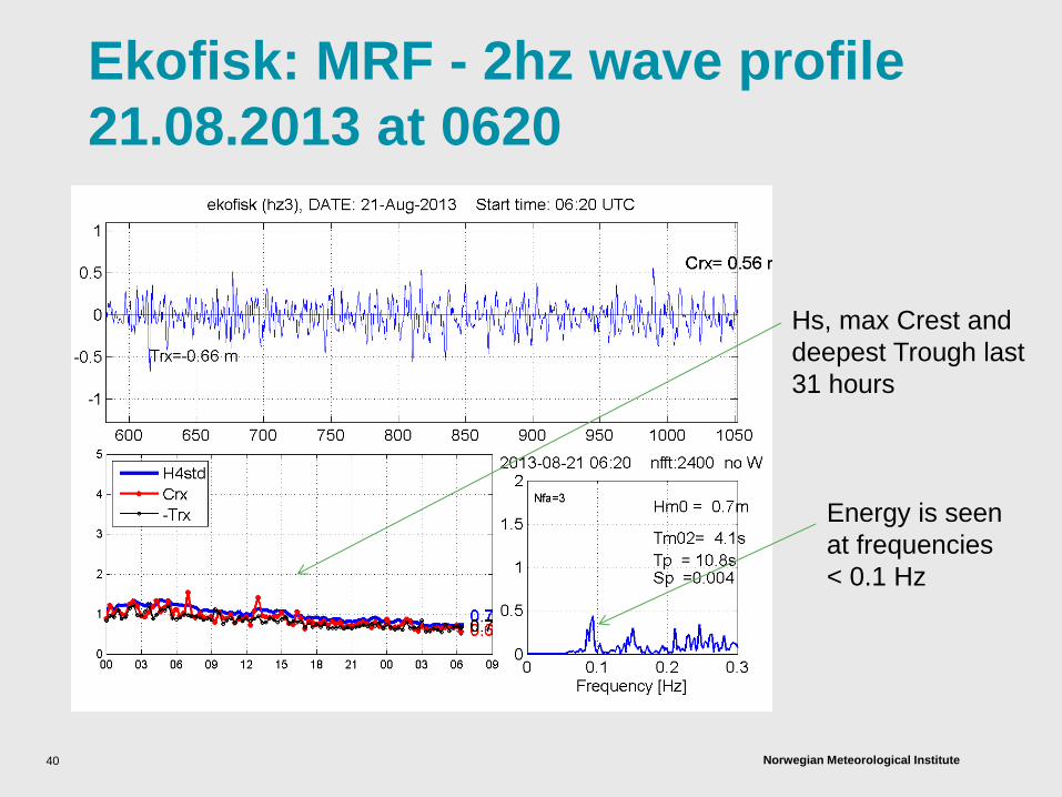
Ekofisk: MRF - 2hz wave profile

21.08.2013 at 0620

40

Energy is seen

at frequencies

< 0.1 Hz

Hs, max Crest and

deepest Trough last

31 hours


Peak period increase coming into

the North Sea 21. Aug 2013, 03 UTC

41

Wave directions

Tp

mslp

Norwegian Meteorological Institute 10.10.2013 Bunntekst 42

Peak period increase coming into the

North Sea 21. Aug 2013, 09 UTC


Peak period increase coming into the

North Sea 21. Aug 2013, 21 UTC


Model prognosis for Ekofisk

44

Swell period

12-14 sec decaying …..

Hs ~0.8-1.2 m

Swell dominans Swell dominans


Take off in the evening

Acknowledgments to

ConocoPhillips Norway for

mounting of the LASAR system at

Ekofisk and for use of data in the

EU project Extreme Seas

Picture by Kristine Gjesdal


END OF PRESENTATION

46

variability of sea state measurements and sensor dependence · the sea floor at the ekofisk field...

Documents