Copyright © 2010 by Richard S. Ruback

Working papers are in draft form. This working paper is distributed for purposes of comment and discussion only. It may not be reproduced without permission of the copyright holder. Copies of working papers are available from the author.

Valuation when Cash Flow Forecasts are Biased Richard S. Ruback

Working Paper

11-036

 

 

Valuation when Cash Flow Forecasts are Biased

Richard S. Ruback Harvard Business School Email: rruback@hbs.edu

This Draft: October 2010

Comments Welcome.

Abstract

This paper focuses adaptations to the discount cash flow (DCF) method when valuing forecasted cash flows that are biased measures of expected cash flows. I imagine a simple setting where the expected cash flows equal the forecasted cash flows plus an omitted downside. When the omitted downside is temporary, the adjustment is to deflate the forecasts and to set the discount rate equal to the cost of capital. However, when the downside is permanent, the adjustment is to deflate the cash flows and to increase the discount rate so that it includes the cost of capital plus the probability of a downside.

 

 

 

I am grateful for comments from the participants at the HBS Finance Brown Bag Seminar and especially to Malcolm Baker, Bo Becker, Kobi Boudoukh, Josh Coval, Mihir Desai, Ben Esty, Robin Greenwood, and Scott Mayfield for helpful discussions and comments on earlier drafts. Part of this research was completed while I was visiting at the Interdisciplinary Center (IDC) in Herzliya, Israel.

1 

  

1. Introduction

Cash flow forecasts are commonly created by extending income and cash flow statements

into the future using historical results as a benchmark. Alternatively, projections can be created

through a more fundamental analysis of perceived future opportunities for the product, the firm,

its divisions, or its industry. Or, the cash flow forecasts can be created by a more qualitative

process. Sometimes, best, worst and base case scenarios are forecast but other times just a single

forecast is created. If the cash flow projections are to be used in a discounted cash flow (DCF)

valuation, the forecasts should equal the expected cash flows. The challenge in practice is that

the cash flows forecasts may be a biased measure of the expected cash flows. To be a measure

of the expected cash flows, the forecasts ought to consider the full range of potential outcomes

and then weigh the resulting cash flows in each outcome by their respective probabilities. While

this exercise occurs in many settings, such as pharmaceuticals, the practice is not universal.

Even when managers attempt to estimate the expected cash flows, there are reasons to

suspect those estimates might not be accurate. When managers forecast a "best case", a "base

case" and a "worst case", there is generally no process for accurately assessing the probabilities

of the various outcomes. And there is likely to be an inherent optimism in the forecast of

managers that are both championing the projects as well as trying to value them. The likely

result is that the forecasted cash flows over-estimate the expected cash flows so that the

forecasted cash flows are an upward biased estimate of the expected cash flows. Finally,

because the environment and the available opportunities change constantly, there is no empirical

basis for evaluating the accuracy of either the cash flow forecasts in the various scenarios or the

2  

  

associated probabilities, making it difficult to empirically adjust the forecasted cash flows

towards an unbiased estimate of expected cash flows.1 

This paper focuses on ways in which the discount cash flow approach can be adapted to

value forecasted cash flows that are biased measures of expected cash flows. I do this by

deriving adjusted discounted cash flow formulas that incorporate the deviations of the forecasted

cash flows from the unobservable expected cash flows. I imagine a simple setting in which the

forecasted cash flows differ from the unobservable expected cash flows in a well-defined way.

Specifically, I assume the expected cash flows equal the forecasted cash flows plus a missing

component. Depending on the characterization of the missing component, I get different

adjustments to the discount cash flow formula.

The idea of adjusting the discounted cash flow formula for inaccurate forecasts is not

novel and those adjustments generally increase the DCF discount rate. Poterba and Summers

(1995) show that managers often increase the discount rate beyond market-based cost of capital

measures and suggest that one reason for this is to account for optimistic cash flow forecasts.

Zenner, Berkovitz and Clark (2009) report that the cash flows used in valuation are typically

derived from base-case scenarios that do not include the “possibility of severe downside

scenarios.” As a result, the base-case cash flow forecasts are not expected cash flows. They

report that “[b]ecause it is challenging to adjust cash flows for downside scenarios, increasing

the internal hurdle rate when evaluating new projects is common practice.”

Venture capital firms also use high discount rates when evaluating potential investments.

Sahlman (2009) describes the “venture capital method” of valuation in which potential

investments are valued by discounting forecasted terminal value, estimated assuming the success

                                                             1 Some firms repeat related projects and use their realized results to adapt forecasts. For example, Marriott Corporation used its historical experience about the variance between forecasted and actual cash flows to adjust its forecasts for subsequent projects. See Ruback (1998).

3  

  

of the project, by discount rates that range from 35% to 80%, with the discount rates decreasing

as the project successfully advance through its stages of development. Sahlman explores several

different explanations for these high discount rates used by venture capitalists, including as an

adjustment for the overly optimistic forecasted cash flow that is higher than the expected cash

flow, by definition, because it is based on the assumption of a successful outcome.

Similarly, valuations of international projects or firms often include a “country risk

premium” as part of the discount rate. The country risk premium is generally not intended as an

adjustment for inflation differences which are included elsewhere or for mis-measurement of

systematic risk. Instead, as shown by Esty (2002), the country risk premium can be interpreted

as an adjustment for over-optimistic forecasted cash flows that ignore downside scenarios related

to political risks such as higher taxes and other forms of expropriation.

Including a company specific risk premium to account for differences between the

forecasted and expected cash flows is generally accepted by valuation professionals. The

publications of the American Society of Appraisers (ASA) and the American Institute of

Certified Public Accountants (AICPA) suggest in their guides to valuation that company specific

risk premium be included in the discount rate as an adjustment for the riskiness of the forecast.

These adjustments are qualitative, at best. The ASA manual explains that “There are few

objective data and no quantitative means of establishing the company-specific risk premium. It

is largely a matter of judgment and experience.” [page 61, v. 5.1 (11/06)]. The AICPA

publication, Understanding Business Valuation, suggests that the company-specific risk

premium should account for “risk elements not covered by the equity risk premium.” It also

reports that there is “no objective source of data to properly reflect or quantify” the company-

specific risk premium, “[t]here are no mystical tables that an appraiser can turn to, nor can the

4  

  

appraiser be totally comfortable with this portion of the assignment” and that it makes “auditors

cringe.”

While the practice of increasing the discount rate in DCF calculations to account for

biased cash flow forecasts is common by practitioners and appraisers, and is used in venture

capital and international project valuations, most traditional academic discussions frown on it.

Brealey, Myers, and Allen (2005) describe these denominator adjustments as “fudge factors” that

managers use because they “fail to give bad outcomes their due weight in cash flow forecasts.”

These discount rate adjustments make the authors “nervous” and they recommend that managers

instead adjust the forecasts so that cash flows used in the DCF calculation are expected values.

In this paper I simply model the expected cash flows as the forecasted cash flows plus a

missing component. I present two different specifications of the missing component in Section

2. I show that the appropriate adjustment to the DCF formula when using forecasted cash flows

depends on the specification of the missing component. In one specification, the appropriate

adjustment is to decrease the forecasted cash flows; in the other specification, however, the

appropriate adjustment is to decrease the forecasted cash flows and increase the discount rate.

Furthermore, the choice of specification has a substantial impact on the estimated value.

In the first specification of the missing component, described in section 2.1, there is a

chance of a downside in which the company or project would realize no cash flow. Each

forecast period is independent in the sense that there is an equal chance of the downside

occurring in each of the forecast periods; whether the downside occurs or not, the chance of a

subsequent downside is unaffected. An example of this type of omitted temporary downside is a

weather-related agricultural loss. I show that in this specification of the missing component, the

appropriate adjustment to the discounted cash flow formula is to reduce the cash flows by

5  

  

multiplying them by the chance that the downside will not occur. The discount rate equals the

cost of capital.

In the second specification of the missing component, described in section 2.2, there is

again a chance of that the company or project will realize no cash flow. However, unlike the

first specification, if the downside occurs, the subsequent cash flows will remain at zero. The

downside is absorbing. In other words, the project gets stuck in the downside and cannot

recover. The downside is permanent. An example of this type of an omitted downside is a

catastrophic technological failure in which the project permanently ceases operation. I show

that in this specification of the missing component, the appropriate adjustment to the discounted

cash flow formula is to reduce the cash flow forecasts as in the first specification and to also

increase the discount rate beyond the cost of capital by adding the chance that the downside will

occur.

The adjustments to the discounted cash flow formula reduce the estimated value of the

projects in both specifications. However, the impact on value is substantially greater when the

project cannot recover from the occurrence of the downside. For example, when valuing a

perpetuity that has a 10% chance of a downside, the value with the temporary specification is

90% of the unadjusted value whereas the value is only 45% of the unadjusted value with an

absorbing downside. Thus, choice of omitted downside has a significant effect on the estimated

value. Section 3 shows how this effect on value varied with the length of the forecast period, the

discount rate and the probability of the downside occurring.

I conclude in Section 4 and offer some recommendations.

6  

  

2. Adjusted discounted cash flow formulas

In this section I derive the adjusted discounted cash flow formulas that can be used to

value forecasted cash flows that are explicitly not expected cash flows. The forecasted cash

flows differ from the expected cash flows by an omitted downside, so that the expected cash

flows equal the forecasted cash flows plus the omitted downside. In the first subsection, I derive

the adjusted DCF formula when the omitted downside is assumed to have an independent chance

of occurring in each forecast period and therefore is temporary. The second subsection derives

the adjusted DCF formula when the omitted downside is instead absorbing in the sense that, if

the downside occurs, it changes the subsequent cash flows so that it is permanent.

2.1. Temporary omitted downside

To keep the analysis as simple as possible, I assume that the forecasted cash flows are

constant through time and perpetual. I define the forecasted cash flows as X in each period2. The

forecasted cash flows by construction are not expected cash flows because X does not include

the possibility of a downside. Suppose that the probability of such a downside is λ and, initially,

that the expected cash flow in that scenario is zero. The chance that such a downside occurs

remains the same in each period and that the occurrence of the downside does not impact future

cash flows. Thus, the downside is independent in the sense that, if it occurs, it is temporary.

Figure 1 diagrams the cash flows in the first three periods. As shown in Figure 1, there is

a (1‐λ) probability of a cash flow of X and a λ probability of a cash flow of zero in period 1. The

expected cash flow in period 1 therefore is:

1( ) (1 ) ( )0 (1 ) .E X X Xλ λ λ= − + = −

                                                           

           [1]

   2 X is the expected cash flow conditional on the downside not occurring.

7  

  

In period 2, there are four potential paths through the outcome diagram in Figure 1 and

the expected cash flow is the probability weighted sum of the cash flows in each of the four

potential outcomes:

[ ] (1 ) (1 ) ( )X X2( ) (1 )(1 ) (1 )( )0 ( )(1 ) ( )( )0

(1 ) .

E X X X

X

λ λ λ λ λ λ λλλ

= − − + − + − +

= −

λλ λ= − − +                                        

[2]

                           

It follows that the expected cash flow in each period t, E(X)t, equals:

2 3( ) (1 ) (1 ) (1 )

(1 ) .

PV Xk k k

Xk

(1 ) (1 ) (1 ) ...X X Xλ λ λ= + + +

+ + +

−=

.

λ

                                          ( ) (1 ) ( )tE X X E Xλ

− − −

= − =   

                                                           

                      [3]                        

In words, the evolution of the cash flows do not change the expected value of subsequent cash

flows which remain at X(1-λ).   

The present value of the cash flows is calculated by discounting the expected cash flows,

E(X), by the appropriate risk adjusted cost of capital which I define as k3:

[4]                          

   

 

Compared to the unadjusted discounted cash flows, the adjusted discounted cash flows will be

lower by the probability of the downside scenario in which the cash flow is zero. In other words,

if there is a 10% chance that the cash flows could be zero, and if the chance of such a downside

stays constant through time, the present value is 10% lower than the unadjusted discounted cash

flow.

The omitted downside used in deriving [4] assumed that there is no cash flow when it

occurs. It is straight-forward, however, to generalize that result to include downsides that have

  3 For simplicity, I assume that the asset betas of the forecasted and downside cash flows are identical so that cost of capital is the same in both the forecasted and downside scenarios.

8  

  

non-zero cash flows. Assuming a forecasted cash flow of XH and an independent omitted

downside in which the cash flow is XL that occurs with probability λ, the expected cash flow is4:

( ) (1 ) .H LE X X Xλ λ= − +                                              [5] 

To obtain the adjusted discounted cash flow formula, the numerator in [4] is simply replaced

with the expected cash flow in [5]:

                                    

(1 )( )

(1 )( )

L H

L H L

X XPV Xk

X X Xk k

λ λ

λ

+ −=

− −= +

                                                       [6]      

This equation for the value of cash flow forecast of XH with an omitted independent

downside cash flow of XL has a familiar interpretation. The first term on the right-hand-side

(RHS) of [6] is the present value of a perpetual expected cash flow of XL. The second term on

the RHS of [6] is the value of a forecasted cash flow of XH-XL that omits a temporary downside

scenario of a cash flow of zero that occurs with probability λ. Thus, the more general

formulation is simply the sum of two parts: the present value of the expected cash flow of XL

plus the present value of a forecast of XH-XL that omits a temporary downside of no cash flows

that occurs with probability λ.

2.2. Permanent omitted downside

Once again assume that the forecasted cash flows by construction are not equal to

expected cash flows because the forecasts omit a downside scenario. Assume that the downside

occurs with probability λ and, initially, that the cash flow in the downside is zero. However,

unlike the downside where the probability of a downside is independent in each period, if this

                                                             4 XH is the expected cash flow conditional on the downside not occurring and XL is the expected cash flow conditional on the downside occurring.    

9  

  

10  

downside occurs, the subsequent cash flows will be zero thereafter. Thus, the downside is

absorbing in the sense that, if it occurs, it is permanent.

Figure 2 shows the evolution of the project over three periods. In the first period, the

expected cash flow is derived as in equation [1]. In the second period, however, the permanence

of the omitted downside scenario reduces the expected cash flow:

2 3(1 ) (1 ) (1 )) ...X X XPV λ λ λ− − −= + + +2 3(

(1 ) (1 ) (1 )

(1 ) ( )

Xk k k

XK

λλ

+ + +

−=

+

( ) (1 )(1 ) (1 )( )0 ( )0 E X X

                       

2

2 (1 ) X

λ λ λ λ λ= − − + − +

3

λ= −                                           [7] 

The expected cash flow in period 3 follows the same pattern:

      3

( ) (1 )(1 )(1 ) (1 )(1 )( )0 (1 )( )0 ( )0

(1 ) .E X X

Xλ λ λ λ λ λ λ λ λ

λ

= − − − + − − + − +

= −  [8]         

By extension, the expected cash flow in period t, Et(X) equals:  

  ( ) (1 )t .tE X Xλ= −                                                           [9]                     

The present value of the cash flows is calculated by discounting the expected cash flows,

E(X), by the appropriate risk adjusted discount rate, k:

                                                  

    [10]                        

   

The adjusted DCF value is lower when the downside is permanent [10] than it is when the

downside scenario is temporary [4]. Both adjusted DCF formulas reduce the cash flow forecast

by the probability of a downside. When the downside is assumed to be temporary, there is no

adjustment to the discount rate. In contrast, when the downside is assumed to be permanent, the

  

probability that the downside will occur is added to the cost of capital. This increases the

discount rate, which decreases the value. In other words, while a 10% chance of a temporary

downside reduces the unadjusted discounted cash flow by 10%, a 10% chance of a permanent

downside scenario reduces the unadjusted discounted cash flow by substantially more than 10%.

The Section 3 presents more details on the relative impact of the adjustments on value.

As with the omitted independent scenario in Section 2.1, it is again straight-forward to

extend [10] to include downsides that have non-zero cash flows. Assuming a forecasted cash

flow of XH and an absorbing omitted scenario in which the cash flow is XL and occurs with

probability λ, the expected cash flow is: 

   ( ) (1 ) (1 (1 ) ) .t tH LtE X X Xλ= − + − − λ                                              [11]       

                                   The discounted value of these expected cash flows equals:

1

(1 ) (1 (1 ) )( ) (1 )

(1 )( ) ( )

t tH L

tt

L H L

X XPV Xk

X X Xk k

λ λ

λλ

∞

=

− + − −=

+

− −= +

+

∑ [12]

                          

Like [6], this formula has a simple interpretation. The first term on the RHS of [12] is the value

of a stream of expected cash flows equal to XL. The second term on the RHS of [12] can be

interpreted using [10] as the value of an asset with a forecasted cash flow equal to (XH - XL) and

a probability of λ of an absorbing downside scenario in which there is no cash flow. Thus, the

more general formulation with a downside scenario cash flow of XL instead of zero is simply the

sum of the two parts: the value of expected cash flows of XL and no omitted downside scenario

plus a forecasted cash flow of (XH - XL) with an omitted downside scenario in which the

probability of no cash flow occurring is λ.   

11  

  

The formula and approach in [12] can be extended to include a variety of alternative

specifications of the downside. For example, the downside could have a lasting impact even

though recovery is possible. Figure 3 diagrams the probabilities and payoffs when the probability

of a downside occurring is λ initially and remains at λ as long as the downside scenario has not

yet occurred. Once the downside occurs, there is a permanent shift downward in the probability

of a subsequent downside. Specifically, the probability of achieving the forecasted cash flow

becomes (1-γ) and the probability of a subsequent downside is γ, where γ is greater than λ.  

Situations that might fit this example include omitting the risk of labor strike where the

subsequent expected cash flows are permanently reduced because of higher wages or the risk that

a market leader will lose its position of dominance and will have lower expected cash flows once

that leadership position is lost.

The expected value of the cash flow is:

    1t tλ ( ) (1 ) (1 ) (1 (1 ) )tE X X Xλ γ −+= − − − −                                               [13] 

The first term on the RHS of [13] is the probability of cash flow of X in period t if no

downside occurs in any prior period. This term is the same as in the expected cash flow in the

absorbing downside [9]. The second term on the RHS of [13] is the expected value of the cash

flow in period t when a downside occurred in a prior period.

The adjusted discounted cash flow formula when the expected cash flows are given by

[13] is:

(1 ) (1 ) (1 )( ) ( )

X XPV Xk k

Xγ λ γλ

− − − −= +

+                          [14]

The formula in [14] can again be interpreted as the sum of two parts. The first-term on the RHS

of [14] is simply the value of a forecast that omits an independent downside that occurs with a

12  

  

probability of γ.  The second-term on the RHS of [14] adds the value of a forecast equal to the

difference between the expected value of the cash flow in the two scenarios with an omitted

absorbing downside with the probability λ.  Of course, when γ=λ, equation [14] simplifies to the 

adjusted DCF with an omitted independent downside with a likelihood of λ. And when γ=1 the

example is equivalent to the absorbing downside so that equation [14] simplifies to [10]. 

In both [12] and [14] the formulas show that the correct approach is to value the forecasts

in two parts. The first part is the expected cash flow conditional on the downside occurring as if

it omits an independent downside so that the value of the first part is the expected cash flow

discounted at the cost of capital. The second part adds the value of a forecast equal to the

difference between the expected cash flows in the forecast and downside scenarios with an

absorbing omitted downside so that the value of the second part is the difference in the expected

cash flows discounted by the cost of capital plus the probability of an absorbing downside. Thus,

the first part adjusts the cash flow and the second part adjusts the cash flow and the discount rate.

The adjusted DCF in [14] is larger than the adjusted DCF in the independent case with

probability γ because the second term on the RHS of [14] is positive when the probability of a

subsequent downside is greater than the probability of an initial downside and the cash flow

forecast is greater than zero. The bigger the difference between the probabilities of a downside

before and after its occurrence, γ ‐ λ, determines the benefit relative to the independent case. The

smaller λ is, holding γ fixed, the larger is the numerator of the second RHS term of [14] and the

smaller is the denominator, both of which increase the DCF value. As γ changes, both the first

and second term of [14] change in opposite directions; an increase in γ decreases the first term

and increases the second. But because the probability of an initial downside appears in the

13  

  

denominator of the second term and not the first, the impact on the first term will be larger than

the impact on the second. Thus, a smaller γ increases the DCF value.   

 

3. Impact of the discounted cash flow adjustments

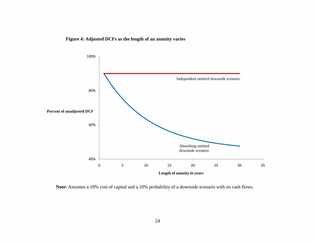
Figure 4 provides a numerical example that gives a sense of the impact of the discounted

cash flow adjustments on valuations. The example assumes a constant forecasted cash flow, a

10% discount rate and an omitted downside that has a likelihood of occurrence of 10% and a

cash flow of zero. The plotted present values are expressed as a percentage of the unadjusted

DCF.

The adjusted DCF when the downside is temporary is 90% of the unadjusted value

because the adjustment simply reduces the forecasted base case cash flow by 10% to the

expected cash flow and values it using the same discount rate. The adjusted DCF when the

downside is permanent, however, has a more significant impact on value that increases as the

number of discounting periods increases; the adjusted DCF in the absorbing downside is 61% of

the unadjusted DCF for a 10-year constant cash flow falling to 48% by year 30.

For a perpetual cash flow, the unadjusted value is:   

1010%

Unadjusted DCF xk

= = = .x x 

Assuming an independent omitted downside scenario, the value of the perpetuity is:

(1 ) .9 ,x x 9

10%Adjusted DCF x

kλ−

= = =  

which is 90% of the unadjusted value. In contrast, assuming the omitted downside is permanent

results in a value of the perpetuity that is 45% of the unadjusted value and half of the value

14  

  

obtained when a temporary downside is assumed:

(1 ) .9 .x x 4.510% 10%

Adjusted DCF xk

λλ

−= = =

+ + 

Thus, while a temporary omitted downside has a constant impact on value as the length

of the annuity increases, a permanent omitted downside has an increasing impact on value as the

length of the annuity increases. The longer the life of the asset being valued, therefore, the more

important is the specification of a temporary or permanent downside.

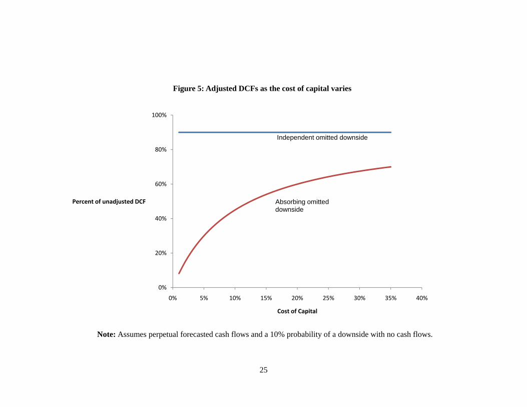
Figure 5 graphically shows the impact of the cost of capital on the adjusted DCFs. The

figure assumes a perpetual forecasted cash flow and an omitted downside that has 10%

probability of occurring and that, if it occurs, the cash flow will have an expected value of zero.

The adjusted DCF is 90% of the unadjusted value regardless of the cost of capital when a

temporary omitted downside is assumed. In contrast, the lower the cost of capital, the larger the

impact of adjusting the DCF for a permanent omitted downside. For example, when the cost of

capital is 5%, the adjusted DCF for the absorbing omitted downside is 30% of the unadjusted

value; when the cost of capital is 10%, the adjusted DCF is 45%; and when the cost of capital is

15%, the adjusted DCF is 54%. Thus, the lower the cost of capital, either because of low real

riskless rates, low inflation, low betas, or low risk premiums, the larger the value consequence of

assuming an permanent omitted downside.

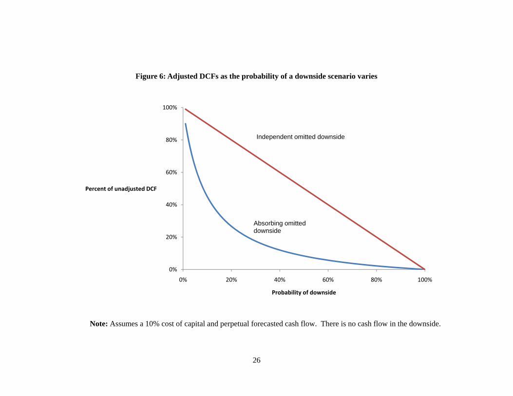
Figure 6 shows the impact of varying the probability of a downside on the adjusted

DCFs. The figure assumes a perpetual forecasted cash flow and an omitted downside that has a

cash flow with an expected value of zero. The assumed discount rate is 10%. The adjusted DCF

is simply equal to the unadjusted value times the probability that the downside will not occur

when the omitted scenario is assumed to be temporary and the corresponding adjusted DCF is a

15  

  

straight line in Figure 2. When the omitted downside is permanent, the probability of a downside

compounds because it is included in the discount rate. At low levels of the probability, an

increase in the probability of a downside has a substantial impact on the adjusted DCF.

The calculations in Figure 6 assume that the probability of a downside is constant through

time. Alternatively, the probability of a downside may decline throughout the life of a project.

For example, technological risks and concerns about over-optimistic projections of demand or

profitability may resolve in the first few years of a project. When the probability of a downside

declines over the life of the project, the value impact of the downside lessens. To gauge the

impact of a declining downside probability over the life of a project, suppose it declines through

time so that:

(1 )ttλ λ δ= −

                          

where  1.   This reduces the probability of a downside and increases the probability of no

downside, especially during the first few years of a project. For example, if λ is 10%, the

probability of no downside without attenuation is 35% through the fifth year of the project. With

a 10% rate of attenuation, the probability of no downside is about 55% through the fifth year;

with a 15% rate of attenuation, it is about 63%; and, with a 20% rate of attenuation the

probability of no downside through year five is almost 70%, which is twice the probability

without attenuation. At the ten-year mark the differences are more pronounced. The probability

of no downside through the tenth year without attenuation is 12%; with a 10% attenuation rate,

the probability is 44%; with a 15% attenuation rate, the probability is 57%; and, with a 20%

attenuation rate, the probability is 67%.

16  

  

The value with a permanent omitted downside with attenuation becomes:

1

(1 (1 ) )( ) (1 )tt .

t t XPV Xk

λ δ∞

=

− −=

+∑  

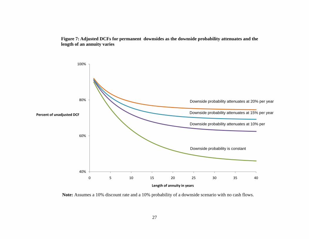
Figure 7 plots the values relative to the unadjusted value for various lengths of an annuity with a

constant probability of a downside and with 10%, 15% and 20% rates of attenuation using a 10%

cost of capital in all of the calculations. The figure shows that the impact of a permanent omitted

downside becomes less important as the probability of the downside occurring attenuates over

the life of the project. The larger the attenuation, the larger is the adjusted DCF as a percent of

the unadjusted value. However, even for relatively larger rates of attenuation such as 20% per

year, the impact is still significant. Omitting a 10% probability of a permanent downside for a

10 year project would still over-estimate the value of the project by roughly one-quarter.5

4. Summary and recommendations

This paper examines adjustments to the discounted cash flow formula to value overly

optimistic forecasts that are upward biased estimates of expected cash flows. I assume that the

forecasts omit a downside scenario so that the forecasts plus the omitted downside equals the

expected cash flows. I show that the characterization of that omitted downside determines the

appropriate adjustment to the DCF formula. I derived the adjusted DCF formulas to show that

the two most common adjustments to DCF for overly optimistic cash flow forecasts have a

conceptual basis.

I show that when the omitted downside is temporary, the appropriate adjustment to the

DCF formula is to deflate the forecasts by the expected downside and to set the discount rate

                                                             5 With a 10% cost of capital, 10% probability of a permanent downside and a 20% attenuation rate, the value of the adjusted NPV is 76% of the unadjusted NPV.

17  

  

equal to the cost of capital. However, when the omitted downside scenario is permanent in the

sense that subsequent cash flows cannot recover once a downside occurs, the appropriate

adjustment is to deflate the cash flows and to increase the discount rate to include the cost of

capital plus the probability that a downside occurs. Thus, there is a reasonable conceptual basis

for both the academic approach of deflating the forecasts and the practitioner approach of

inflating the discount rate. The appropriate approach depends on the characterization of the

omitted downside as either temporary or permanent.

In practice, omitted downsides are unlikely to be easily characterized as temporary or

permanent, although those surely do occur. Temporary downsides include, for example, weather

related events; a frost that destroys an orange crop can occur in any year but its occurrence does

not change the probability of a future frost. Applying the adjusted DCF for the temporary

downside, the appropriate value is simply the forecast assuming no frost times the probability

that a frost does not occur. Other projects may omit a permanent absorbing downside where

there is no subsequent recovery once a downside occurs. A venture capital firm could, for

example, omit the chance of a catastrophic technological failure in which there are no subsequent

project cash flows. Such a project would be appropriately valued using the DCF adjusted for a

permanent absorbing downside by discounting the expected cash flow conditional on no

technological failure times the probability that the technological failure does not occur

discounted by a rate that equals the sum of the cost of capital and the probability of a

technological failure.

More generally, forecasts may omit downsides that do not neatly match either the

temporary or permanent downsides that I model. When that occurs, one choice is to model the

difference between the forecasted cash flows and their expected values, and then derive an

18  

  

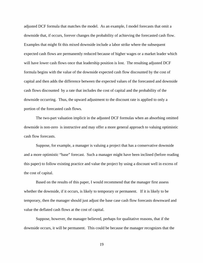
adjusted DCF formula that matches the model. As an example, I model forecasts that omit a

downside that, if occurs, forever changes the probability of achieving the forecasted cash flow.

Examples that might fit this mixed downside include a labor strike where the subsequent

expected cash flows are permanently reduced because of higher wages or a market leader which

will have lower cash flows once that leadership position is lost. The resulting adjusted DCF

formula begins with the value of the downside expected cash flow discounted by the cost of

capital and then adds the difference between the expected values of the forecasted and downside

cash flows discounted by a rate that includes the cost of capital and the probability of the

downside occurring. Thus, the upward adjustment to the discount rate is applied to only a

portion of the forecasted cash flows.

The two-part valuation implicit in the adjusted DCF formulas when an absorbing omitted

downside is non-zero is instructive and may offer a more general approach to valuing optimistic

cash flow forecasts.

Suppose, for example, a manager is valuing a project that has a conservative downside

and a more optimistic “base” forecast. Such a manager might have been inclined (before reading

this paper) to follow existing practice and value the project by using a discount well in excess of

the cost of capital.

Based on the results of this paper, I would recommend that the manager first assess

whether the downside, if it occurs, is likely to temporary or permanent. If it is likely to be

temporary, then the manager should just adjust the base case cash flow forecasts downward and

value the deflated cash flows at the cost of capital.

Suppose, however, the manager believed, perhaps for qualitative reasons, that if the

downside occurs, it will be permanent. This could be because the manager recognizes that the

19  

  

occurrence of the downside could reveal persistent over-optimism about the economic

environment, the success of the technology or the popularity of the project. Whatever the cause,

the manager believes that the occurrence of the downside signals permanently lower cash flows.

The manager still shouldn’t value the base case cash flow at an inflated discount rate. Instead,

the manager should value the project as the sum of two parts. In the first part, the downside cash

flows are discounted at the cost of capital. In the second part, the difference between the base

and downside forecasts should be discounted at a rate that equals sum of the cost of capital and

the probability that the downside will occur. This of course results in a higher value – and a

better decision -- than following the manager’s initial inclination of simply discounting the over-

optimistic cash flows by an inflated discount rate.

   

20  

  

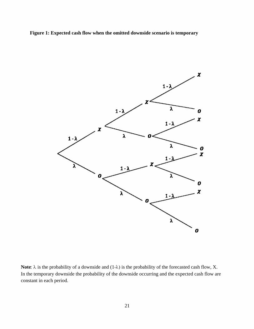
Figure 1: Expected cash flow when the omitted downside scenario is temporary

 

 

 

 

 

     

Note: λ is the probability of a downside and (1‐λ) is the probability of the forecasted cash flow, X. In the temporary downside the probability of the downside occurring and the expected cash flow are constant in each period.

21  

  

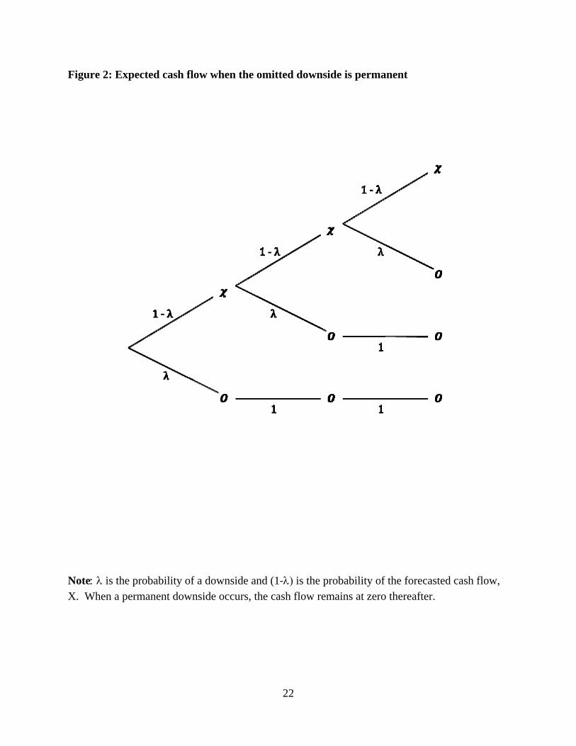
Figure 2: Expected cash flow when the omitted downside is permanent

  

 

 

 

 

 

Note: λ is the probability of a downside and (1‐λ) is the probability of the forecasted cash flow, X. When a permanent downside occurs, the cash flow remains at zero thereafter.   

22  

  

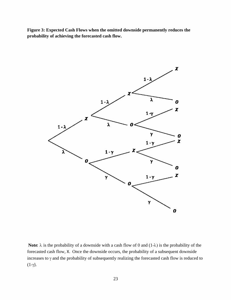
Figure 3: Expected Cash Flows when the omitted downside permanently reduces the probability of achieving the forecasted cash flow. 

 

 

 

 

 

 Note: λ is the probability of a downside with a cash flow of 0 and (1‐λ) is the probability of the forecasted cash flow, X.  Once the downside occurs, the probability of a subsequent downside increases to γ and the probability of subsequently realizing the forecasted cash flow is reduced to (1‐γ). 

23  

40%

60%

80%

100%

0 5 10 15 20 25 30 35

Percent of unadjusted DCF

Length of annuity in years

Figure 4: Adjusted DCFs as the length of an annuity varies

Independent omitted downside scenario

Absorbing omitteddownside scenario

Note: Assumes a 10% cost of capital and a 10% probability of a downside scenario with no cash flows.

24 

 

0%

20%

40%

60%

80%

100%

0% 5% 10% 15% 20% 25% 30% 35% 40%

Percent of unadjusted DCF

Cost of Capital

Figure 5: Adjusted DCFs as the cost of capital varies

Independent omitted downside

Absorbing omitteddownside

Note: Assumes perpetual forecasted cash flows and a 10% probability of a downside with no cash flows.

25 

 

  

26  

 

0%

20%

40%

60%

80%

100%

0% 20% 40% 60% 80% 100%

Percent of unadjusted DCF

Probability of downside

Figure 6: Adjusted DCFs as the probability of a downside scenario varies

Independent omitted downside

Absorbing omitteddownside

Note: Assumes a 10% cost of capital and perpetual forecasted cash flow. There is no cash flow in the downside.

 

  

27  

 

40%

60%

80%

100%

0 5 10 15 20 25 30 35 40

Percent of unadjusted DCF

Length of annuity in years

Figure 7: Adjusted DCFs for permanent downsides as the downside probability attenuates and the length of an annuity varies

Downside probability is constant

Note: Assumes a 10% discount rate and a 10% probability of a downside scenario with no cash flows.

Downside probability attenuates at 10% per

Downside probability attenuates at 15% per year

Downside probability attenuates at 20% per year

  

References

Allen, Franklin, Richard Brealey, and Stewart Meyers. Principles of Corporate Finance. Boston: McGraw-Hill/Irwin, 2006.

American Society of Appraisers. “Business Valuation.” American Society of Appraisers website. http://www.appraisers.org/ASAHome.aspx, accessed August 2009.

Berkovitz, Tomer, Clark, John, and Zenner, Mark, “Creating Value Through Best-In-Class Capital Allocation”. Journal of Applied Corporate Finance 21 (Fall 2009): 89-96.

Esty, Benjamin C., and Millet, Matthew M. “Petrolera Zuata, Petrozuata C.A.” HBS No. 299-012. Boston: Harvard Business School Publishing, 1998, rev. 2002.

Poterba, James M., Summers, Lawrence H., “A CEO Survey of U.S. Companies’ Time Horizons and Hurdle Rates”. MIT Sloan Management Review 37 (October 15, 1995): 43-53.

Ruback, Richard S. “Marriot Corporation: The Cost of Capital.” HBS No. 298-101. Boston: Harvard Business School Publishing, 1998.

Sahlman, William A., and Scherlis, Daniel R. “Method for Valuing High-Risk, Long-Term Investments: The ‘Venture Capital Method’”. HBS No. 288-006. Boston: Harvard Business School Publishing, 2009.

Trugman, Gary R. Understanding Business Valuation. Lewisville, TX: American Institute of Certified Public Accountants, 2007.

 

 

 

 

 

 

 

 

28