an analysis of discounted cash flow (dcf) approach to ... · pdf filean analysis of discounted...
TRANSCRIPT
An analysis of discounted cash flow (DCF) approach
to business valuation in Sri Lanka by Thavamani Thevy Arumugam Matriculation Number: 8029
This dissertation submitted to St Clements University as a requirement for the award of the degree of Doctor of Philosophy
in Financial Management
September 2007

Table of Contents Chapter 1 Introduction .............................................................................................5
1.1 Background.......................................................................................................5 1.1.1 wealth maximization ...............................................................................5
1.2 Concept of an investment ............................................................................6 1.3 Future/Present value of money ....................................................................7 1.4 Discounted cash flow (DCF)..........................................................................8
1.4.1 History of discounted cash flow (DCF) .................................................9 1.5 Risk in context ................................................................................................ 10 1.6 Valuation of a business................................................................................ 12 1.7 Problem discussion........................................................................................ 13
1.7.1 Why do these valuations differ? ......................................................... 13 1.7.2 How does one know which of these values is the most accurate?............................................................................................................................. 13
1.8 Purpose............................................................................................................ 15 1.9 Previous research and potential contribution........................................ 16 1.10 Industry and economic background..................................................... 17
Chapter 2 Literature review.................................................................................. 22 2.1 The investment process ............................................................................... 22 2.2 Risk attitude and perspective .................................................................... 23
2.2.1 Fundamentals of risk management................................................... 23 2.2.2 An approach to risk management.................................................... 25
2.3 Valuation ........................................................................................................ 27 2.3.1 Why is business valuation important?................................................ 27
2.4 Valuation models.......................................................................................... 27 2.5 Asset based valuation ................................................................................. 28
2.5.1 Value of assets........................................................................................ 29 2.5.2 Liabilities ................................................................................................... 30
2.6 Absolute valuation or discounted cash flow (DCF) models................ 30 2.6.1 Incorporate financial and non-financial performance data...... 33 2.6.2 Free cash flow (FCF) discount models .............................................. 35 2.6.3 Calculating the terminal value........................................................... 42 2.6.4 Calculating the discount rate............................................................. 43 2.6.5 Country risk and cost of capital.......................................................... 48 2.6.6 Calculating total enterprise value (EV)............................................. 54 2.6.7 Calculating the value of equity (Ve) ................................................. 55 2.6.8 How do the analysts value a business that is losing money?....... 55 2.6.9 Pros and cons of discounted cash flow DCF................................... 57
2.6.10 Summary................................................................................................ 58 2.7 Discounted dividend model....................................................................... 58 2.8 Relative valuation ......................................................................................... 60
2.8.1 First principles: ......................................................................................... 60 2.8.2 What is relative valuation?................................................................... 62 2.8.3 Reasons for popularity .......................................................................... 62 2.8.4 Potential pitfalls ...................................................................................... 63
2.9 Reconciling relative and discounted cash flow valuations ................ 63 Chapter 3 Methodology ....................................................................................... 65
3.0 Method approaches.................................................................................... 65 3.1 Inductive or deductive approach............................................................ 65 3.2 Quantitative and qualitative approach.................................................. 65 3.3 Research approach..................................................................................... 66 3.4 Research design............................................................................................ 66 3.5 Data collection methods............................................................................ 67
3.5.1 Sample ..................................................................................................... 67 3.6 Modes of data collection ........................................................................... 67
3.6.1 Advantages of questionnaire ............................................................. 68 3.6.2 Disadvantages of questionnaire ........................................................ 68
3.7 Deductive approach................................................................................... 68 3.8 After the interviews, the following steps were taken: ........................... 71 3.9 Reliability and validity of the data............................................................ 71 3.10 Statement of hypothesis............................................................................ 72 3.11 Statistical techniques used in the analysis ............................................ 72 3.12 Summary ....................................................................................................... 72
Chapter 4 Results and discussion ........................................................................ 73 4.0 Introduction.................................................................................................... 73 4.1 Descriptions of participants ........................................................................ 73 4.2 Participants’ views ........................................................................................ 73
4.2.1 Valuation techniques............................................................................ 74 4.2.2 SWOT analysis.......................................................................................... 75 4.2.3 Financial forecasts................................................................................. 76 4.2.4 Terminal value......................................................................................... 78 4.2.5 Cost of debt ............................................................................................ 80 4.2.6 Risk free rate............................................................................................ 81 4.2.7 Risk premium ........................................................................................... 81 4.2.8 Beta estimate.......................................................................................... 82 4.2.9 Cost of equity.......................................................................................... 83 4.2.10 Discount rate......................................................................................... 84 4.2.11 Responses to open questions............................................................ 84
4.3 Inferential statistics ........................................................................................ 95

4.3.1 Tables 1 (r) to v (r) .................................................................................. 97 4.4 Analysis of hypothesis................................................................................. 101 4.5 Discussions .................................................................................................... 102
4.5.1 Risk and uncertainty............................................................................ 107 4.5.2 Valuation of businesses under distress............................................. 112 4.5.3 Adapting discounted cash flow valuation to distress situations 114 4.5.4 Valuing high growth businesses........................................................ 119
Chapter 5 Recommendations and implications ........................................... 125 5.1 Introduction.................................................................................................. 125 5.2 Summary ....................................................................................................... 125 5.3 Recommendations..................................................................................... 127 5.4 Conclusion.................................................................................................... 135 5.5 Further research .......................................................................................... 137
Appendices............................................................................................................ 138 Glossary............................................................................................................ 138 Questionnaire ................................................................................................. 290

Chapter 1 Introduction
1.1 Background Financial management is broadly concerned with the acquisition and use of
funds by a firm. Corporate finance theory has developed around a goal of
shareholder wealth maximization.
Evolution of the corporate financial objective:
Until 1921, the firms did not see any need for stating financial objectives. The
corporate financial objective since then has grown into three phases.
Profit maximization objective
Social responsibility of business
Shareholder wealth maximization
During the time of debate on the social responsibility of business, a few
researchers and thinkers put forward various arguments. That was essentially a
struggle for developing a more acceptable objective statement with time;
shareholder wealth maximization and shareholder value became universally
accepted financial statements for businesses.
1.1.1 Wealth maximization The debate around ‘profit maximization’ and ‘social responsibility’ led to finding a
more logical expression of corporate objectives. This pursuit led to the theory of
shareholder wealth maximization. David Durand and Lutz (1952) introduced the
concept of shareholder wealth maximization. They observed that the goals of
profit maximization as well as wealth maximization are consistent with each other
only under two conditions:
(1) Investment takes place in tiny increments and
(2) Where there is certainty in getting the return on investment
The wealth maximization goal is based on discounting, while putting forth is
macro-economic theory of interest introduced by Alfred Marshall in 1930. Keynes
used the discounting factor in 1936 in his concept of marginal efficiency of
capital.
The shareholders’ wealth maximization goal, thus, reflects the magnitude, timing
and risk associated with the cash flows expected to be received in the future by
shareholders.
1.2 Concept of an investment An investment is the outlay of a sum of money in the expectation of a future
return. This compensates for the original outlay as well as to cover the inflation,
interest foregone and risk. An investment today will determine the firm’s strategic
position many years hence.
Capital budgeting is primarily concerned with sizable investments in long-term
assets. These assets may be tangible items such as property, plant & machinery
or intangible ones such as new technology, patents or trademarks. Investments
in processes such as research, design, development and testing through which
new technology and new products are created may also be viewed as
investments in intangible assets.
Firms operate in a dynamic environment therefore; they must continually make
changes in different areas of their operations in order to meet the challenges of
the changing environment. The strategic need of the firm will determine amongst
other things which investment meet the strategic objectivity. By analysing the
strengths, weaknesses, opportunities and threats (SWOT) of the firm and
external factors such as political, economical, social and technological (PEST)
affecting the firm the management will be able to come to an optimal decision.

The net benefits of investment depend upon the quality of investment decisions.
The quality is judged through the weighing of benefits against the risks and
uncertainties. The net benefit of the project will be a function of
(a) The risks involved (b) the ability to generate synergy, and (c) the firm’s
internal control and pro-activeness.
1.3 Future/Present value of money Investment, financing and dividend decisions have significant impact on the firm’s
valuation. A key concept underlying valuation is the value of money based on
time.
Money has time value. An investment of one rupee today would grow to (1+r) a
year hence. (r is the rate of return earned on the investment)
In an inflationary period, a rupee today represents a greater real purchasing
power than a rupee a year hence. This is due to opportunity cost and risk over
time.
Many financial problems involve cash flows occurring at different points of time.
For evaluating such cash flows, an explicit consideration of time value of money
is required. The value of the present investment on a future date to the time
value of money is called the future value of money.
The concept of discounting is the reverse of compounding; using the
compounding process, the future value of today’s money can be found at a given
rate of interest. By discounting, the present value of a future cash flow can be
found. The formula for discounting can be obtained by interchanging the sides of
the compounding formula.
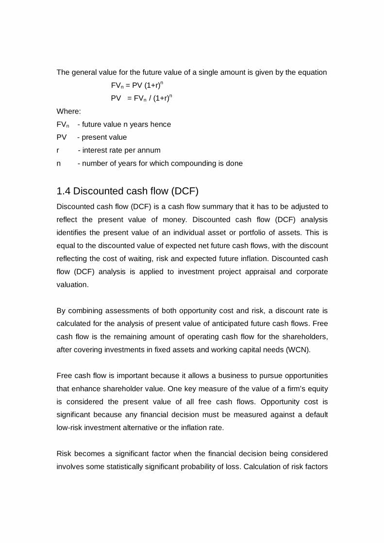
The general value for the future value of a single amount is given by the equation
FVn = PV (1+r)n
PV = FVn / (1+r)n
Where:
FVn - future value n years hence
PV - present value
r - interest rate per annum
n - number of years for which compounding is done
1.4 Discounted cash flow (DCF) Discounted cash flow (DCF) is a cash flow summary that it has to be adjusted to
reflect the present value of money. Discounted cash flow (DCF) analysis
identifies the present value of an individual asset or portfolio of assets. This is
equal to the discounted value of expected net future cash flows, with the discount
reflecting the cost of waiting, risk and expected future inflation. Discounted cash
flow (DCF) analysis is applied to investment project appraisal and corporate
valuation.
By combining assessments of both opportunity cost and risk, a discount rate is
calculated for the analysis of present value of anticipated future cash flows. Free
cash flow is the remaining amount of operating cash flow for the shareholders,
after covering investments in fixed assets and working capital needs (WCN).
Free cash flow is important because it allows a business to pursue opportunities
that enhance shareholder value. One key measure of the value of a firm’s equity
is considered the present value of all free cash flows. Opportunity cost is
significant because any financial decision must be measured against a default
low-risk investment alternative or the inflation rate.
Risk becomes a significant factor when the financial decision being considered
involves some statistically significant probability of loss. Calculation of risk factors
beyond opportunity cost can often be very complex and imprecise, requiring the
use of actuarial analysis methods and in-depth market analysis. When risk is
included in discounted cash flow (DCF) analysis it is generally done so according
to the premise that investments should compensate the investor in proportion to
the magnitude of the risk taken by investing. A large risk should have a high
probability of producing a large return or it is not justifiable.
1.4.1 History of discounted cash flow (DCF) Following the stock market crash of 1929, discounted cash flow (DCF) analysis
gained popularity as a valuation method for stocks. Irving Fisher in his 1930
book, ”The Theory of Interest” and John Burr William’s 1938 text ‘The Theory of
Investment Value’ first formally expressed the discounted cash flow DCF method
in modern economic terms.
Later Gordon (1962) extended the William model by introducing a dividend
growth component in the late 1950’s and early 1960’s. The dividend DIV
continues to be widely used to estimate the value of stock.
In recent years, the literature for estimating the value of a firm and the value of
equity has been expanded dramatically. Copeland, Koller and Murrin (1990,1994,
2000), Rappaport (1988, 1998), Stewart (1991), and Hackel and Livnat (1992)
were current pioneers in modelling the free cash flow to the firm, which is widely
used to derive the value of the firm.
Recently, Copeland, Koller and Murrin (1994) and Damodaran (1998) introduced
an equity valuation model based on discounting a stream of free cash flows to
equity at a required rate of return to shareholders. In addition, Damodaran (2001)
provides several approaches to estimate the value of a firm for which there are
no comparable companies, no operate earnings and a limited amount of cash
flow data. Fama’s (1970) efficient market research challenged the validity of
intrinsic valuation models.
1.5 Risk in context Today world is in a social and political uncertainty. Globalisation is a major factor
in business. The business environment is no longer limited to the country where
it operates. Competition for today’s businesses can come from all the countries
around the globe. Today’s management teams in order to work efficiently and
effectively to cope up with the dynamic change environment need to better,
faster, leaner and quicker on their feet than ever before.
The pace of technological change suggests that this is likely to continue well
beyond the near future and it is clear that standing still is not an option. Only
those organisations that adapt well will prosper; change management becomes
both a business necessity and an art. The true measure of a business success is
the rate at which it can improve its range of products, services and the way it
produces and delivers them.
The reason why risk is so difficult to determine is the varied and uncertain extent
to which business players’ act to influence the outcome. Risk may be defined as
uncertainty about a possible future change, either beneficial or adverse. It is
however different to uncertainty since it can be predicted on a mathematical
basis whereas uncertainty cannot.
The term risk management is applied in a number of diverse disciplines. Too
many social analysts, politicians and academics it is the management of
environmental and nuclear risks, those technology generated macro risks that
appear to threaten our existence.
To bankers and financial officers it is the sophisticated use of such techniques as
currency hedging and interest rate swaps. To insured buyers and sellers it is
coordination of insurable risks and the reduction of insurance costs. To hospital
administers it may mean quality assurance. To safety professionals it is reducing
accidents and injuries.

Risk management is a discipline for living with the possibility that future even to
may cause adverse effects. Risk management means a course of action planned
to reduce the risk of an event occurring and minimizing or containing the
consequential effects should that event occur. In order to achieve this, a risk
management policy should be put in place.
Risk management involves the identification, measurement and economic control
of risks and developing strategies to manage the risk that threaten the assets
and earnings of the institution. The management of any loss-producing event,
which occurs pre-emergency, emergency handling and recovery, is contingency
planning, whereas the process of restoring operations and minimising the loss
associated with an occurrence is disaster recovery.
In ideal risk management, a prioritisation process is followed whereby the risks
with the greatest loss and the greatest probability of occurring are handled first,
and risks with lower probability of occurrence and lower loss are handled later. In
practice, the process can be very difficult when balancing between risks.
Risk management also faces a difficulty in allocating resources properly. This is
the idea of opportunity cost. Resources spent on risk management could be
instead spent on activities that are more profitable. Again, ideal risk management
spends the least amount of resources in the process while reducing the effects of
risks as much as possible.
Learn from your mistakes is an admonition for losers. Successful people learn
from others’ mistakes and thereby avoid their own. As business become
increasingly complex, it is becoming more difficult for CEOs to know what
problems might lie in wait. Therefore, they need someone systematically to look
for potential problems to design safeguards in order to minimise potential
damage. In any event, risk management is becoming increasingly important.

Risk management is seen as the answer for developing the business ability to
anticipate the unexpected. Businesses can identify and analyse the risk and then
can use their core competences to manage them. Businesses can turnaround
plenty of threats into opportunities if they really assess the risks better than their
rivals do.
Risk management should not be looked at another task for today’s business
players to fit into an already overcrowded business schedule. Businesses have to
adapt ways of prioritising the schedule, deploying people and capital more
productively. The important issue is to focus on the uncertainties of future and to
be able to identify and handle them. Risk management can help to ensure that
they reach the successful goal eventually.
1.6 Valuation of a business A business valuation is the process of determining the intrinsic value of common
stock. The valuation process includes understanding the business, analysing the
industry, determining a methodology and generating a report.
In a globalise dynamic business world, valuation is gaining momentum in
emerging markets for mergers, acquisitions, joint ventures, restructuring and the
basic task of running businesses to create value. Yet valuation is much more
difficult in these environments because buyers and sellers face greater risks and
obstacles than they do in developed countries.
In 1997, the risks and obstacles had been so serious in the emerging markets of
East Asia. This Asian financial crisis weakened a mass of companies and banks
and led to a surge in merger and acquisition activity, giving valuation practitioners
a good chance to test their skills. The findings of valuation of companies in
emerging markets clearly suggest that market prices for equities do not take into
account the commonly expected country risk premium. If these premiums were
included in the cost of capital, the valuation would be 50 to 90 percent lower than

the market values. (Asian Development Outlook 2000, Asian Development Bank
and Oxford University Press, p. 32)
In order for the stock market to function, a belief in valuation techniques of
individual firms is necessary. Without a valuation model to estimate value,
investors would not be able to arrive at conclusions on what price to buy or sell
an asset. When inspecting different analysts’ results of specific business
valuation, the value often differs.
1.7 Problem discussion 1.7.1 Why do these valuations differ? This is because different valuation techniques used by different analysts and the
inputs plugged into the valuation techniques differ between the analysts. Since
the analysts have diverse views of the future of the business, their forecasts will
differ, hence the recommended values differ.
1.7.2 How does one know which of these values is the most
accurate? It is not possible to determine the correct value because of risks and
uncertainties involved in carrying out businesses. Therefore, a present needs to
improve the tools used by analysts in valuing their businesses.
In order to understand valuation, two main concepts of value must be
understood. First, the commonly accepted theoretical principle to value any
financial asset is the discounted cash flow (DCF) methodology. An asset is worth
the amount of all future cash flows to the owner of this asset discounted at an
opportunity rate that reflects the risk of the investment. This fundamental
principle does not change and is valid through time and geography. A valuation
model that best converts this theoretical principle into practice should be the
most useful.

Based on the first concept, the second concept states that valuation is an
inherently forward looking in a business. Valuation requires an estimate of the
present value of all expected future cash flows to shareholders. In other words, it
involves looking into an uncertain future and making an educated guess about
the many factors determining future cash flows. Since the future is uncertain,
intrinsic value estimates will always be subjective and imprecise. Better models
and superior estimation techniques may reduce the degree of inaccuracy, but no
valuation technique can be expected to deliver a single correct intrinsic value
measure.
These main concepts illustrate that there are few things more complex than the
valuation of businesses. Thousands of variables affect the future cash flows of a
company and thus the value of a business. Most variables are known, but very
few are understood; they are independent and related, they are measurable, but
not necessarily quantitative and they affect business values alone and in
combination.
A continuous need is to improve the tools used by analysts when valuing firms.
This dissertation aims to contribute to the continuous process. There are several
opinions on what creates value in a business. Therefore, there are different
approaches to estimate the value of a firm. It is a huge task to do research on all
approaches. In this dissertation, a brief discussion was made on selected core
value techniques and the focus is on discounted cash flow (DCF) value model
approach.
Discounted cash flow (DCF) method is the mostly used fundamental method in
business valuation (Perrakis, 1999), consequently the basic problem that this
study is faced with is; how can improvements to the discounted cash flow (DCF)
model, as it is used to value firms, be achieved?

In order to show how analysts can improve the way they apply the discounted
cash flow (DCF) model and how they report their results, thorough understanding
of the discounted cash flow (DCF) model and the context in which it is used is
necessary. In order to achieve this, analyst has to ask the question; what are the
weaknesses and limitations of the discounted cash flow (DCF) model. The
discounted cash flow (DCF) method is used as a management tool in decision
making of the businesses.
The discounted cash flow (DCF) model depends on two inputs; the numerator,
which is an estimated future cash flow and the denominator i.e. discount rate
(weighted average cost of capital). The output of the model is dependent on
these two inputs. How to calculate the denominator are the major concern of
some scientific reports (Bohlin, 1995) as well as the topic of large discussions in
financial text. (Copeland, 2001, Perrakis, 1991 and Ross, 1991)
To summarise the problem discussion; the thesis is conducted in order to find
reasons behind problem areas in the discounted cash flow (DCF) approach to
firm valuation, as well as how improvements can be made to these areas.
This will be accomplished by conducting,
1) A literature study of related academic theories, mathematical models in
general, the discounted cash flow (DCF) model in particular, forecasting
models of revenue, risks, uncertainties involved, cost of capital, discount
rate to be used on the free cash flows in order to project the present
values.
2) Questionnaire survey and personal interviews of 63 organisations
1.8 Purpose The purpose of this study is to analyse the theories and examine the approaches
of business valuation models. Identifying the key inputs used in the valuation
models, and then to find out the methods of forecasting these inputs with greater

degree of accuracy. This will be accomplished by a literature study and a
subsequent questionnaire survey.
The purpose of the literature study is to analyse the use of the discounted cash
flow method as it is used in firm valuation. The aim is to probe into the
weaknesses of the method and the reasons behind the problem areas. Further,
the study will be conducted to find reasons and arguments to solutions of these
problems
The purpose of the subsequent questionnaire survey is to prove whether the null
hypothesis is true or false and to expose important implications of empirical
weaknesses and limitations of the discounted cash flow (DCF) model.
The null hypothesis H0 states that the different techniques of valuation of
businesses will produce the same results.
The alternate hypothesis H1 assumes that different techniques of valuation of
businesses will not produce the same results.
1.9 Previous research and potential contribution Today the discounted cash flow (DCF) model is the most commonly used tool
among financial analysts when valuing a firm. It is documented that almost fifty
percent of all financial analysts use a discounted cash flow (DCF) method when
valuing potential objects to acquire (Hult, 1998). In a study Absiye & Diking
(2001) found that all seven of their respondents, which were analysts, use the
discounted cash flow (DCF) model when they were conducting a firm valuation,
the other valuation models were just used as complements to the valuation done
by the discounted cash flow (DCF) method.
Quite a lot of other studies have been conducted on business valuation. Some of
these focus on the different methods that are used to conduct valuations. They
investigate compare and contrast which model, analysts use and how they look
at these models. For example, see Absiye and Diking (2001) and Carlsson
(2000).
Others centre on how one or more of the valuations models are constructed see
Eixmann (2000), still others conduct case studies where a valuation approach,
frequently the discounted cash flow (DCF) model, is applied to a special case.
Example of such research is Bin (2001).
Firstly, the focus is on one model, the discounted cash flow (DCF) model, but the
whole context of the valuation process is in focus. Furthermore, the investigation
is directed towards finding areas to improve within the discounted cash flow
(DCF) approach and the ways to make improvements in these areas.
1.10 Industry and economic background The legal underpinning for investing in Sri Lanka is law no 4 of 1978 as amended
by acts nos. 43 of 1980, 21 of 1983 and 49 of 1992 the Board of Investment law
(the BOI Law), regulation No 1 of 1978 and regulation No 1 of 1991.
Sri Lanka’s investment policy statement (IPS) of 31 October 1990 opened the
economy to large-scale foreign investment and effectively defined the ground
rules for off shore investors. IPS identified the industrial sectors the Sri Lankan
government would most like to stimulate, simply encourage or regulate tightly.
The BOI is the sole authority for the approval and facilitation of foreign direct
investment in Sri Lanka.
In 2005, the industrial sector contributed 36% to the overall growth. Industry
sector registered a growth of 8.3% in 2005. The major contribution to the growth
in factory industries arose from four of the nine major industrial categories,
textile, apparel and leather products; food, beverages and tobacco products;

chemical, petroleum, rubber and plastic products; and non-metallic mineral
products.
These industries benefited from the global economic recovery, increased
domestic consumer demand, the low interest rate regime, continuation of the
ceasefire and improvements in basic industrial infrastructure facilities. The
competitiveness in exports was facilitated by the improvement in productivity,
rationalisation of production costs and depreciation of the exchange rate.
Foreign direct investment inflows to Sri Lanka rose by 22.6% in US Dollar terms
during 2005. Industrial sector growth, particularly the growth in the textile and
garments sub sector, continued despite the uncertainty that prevailed in early
2005 and the surge in oil prices to historically high levels.
Inflation, which was 15.9% in February 2005 declined to 8% in December 2005.
The average annual inflation in 2005 was 11.6%. By responding well to monetary
policy measures and supported by favourable developments in aggregate supply
were the reasons behind for the inflation rate to decline beginning of the year to
end of the year.
The Indo-Lanka Free Trade agreement has opened up the huge Indian Market to
a large number of Sri Lankan manufactured goods and has thus generated
greater interest on the part of foreign companies. This development will lead to
considerable employment generation and earnings of foreign exchange for Sri
Lanka.

Composition of Industrial Production 2005
12345678910
Category Percentage
1 Food beverage and tobacco products 22% 2 Textile, wearing apparel and leather products 39% 3 Wood and wood products 1% 4 Paper and paper products 2% 5 Chemical, petroleum, rubber &plastic products 21% 6 Non metallic mineral products 8% 7 Basic metal products 1% 8 Fabricated metal products 4% 9 Others 2%
Source: Annual Report 2005, Central Bank of Sri Lanka Value of Investment
YearsRs in billion
2001 502002 602003 1402004 1202005 70

Value of Investment Rs in billion
0
20
40
60
80
100
120
140
1 2 3 4 5
Years
Source: Annual Report 2005, Central Bank of Sri Lanka The key to economic and social growth in all countries developed or developing
is better management in all sectors, which includes agriculture, industry, public
works, education, public health and govt. In recent years, investigators have
studied waste and mismanagement on a wide range of projects. There is a
growing awareness of the need to improve both the productivity and quality of the
projects. The need to understand the impacts of various projects on the
environment and public health is intimately related to project planning and
management.
Effective management of projects is vital for the development of any economy
because development itself is the effect of a series of successfully managed
projects. This makes valuation of a business is extremely important problem area
for a developing economy such as ours in Sri Lanka.

Unfortunately, many businesses experience mergers, acquisitions, restructuring
and litigation due to a variety of reasons. To remedy the situation, a business
valuation technique has to be meticulously planned, effectively implemented and
professionally managed to achieve the objectives of shareholders wealth
maximisation. Scientific techniques of valuation can play a major role in
streamlining the management of businesses.

Chapter 2 Literature review 2.1 The investment process Karl Marx (Marx, 1887) in his book ‘Capital’ uses a remarkably simple equation to
explain the capitalist system: M-C-M. The capitalist starts with money (M) that is
the essence for investment process. Investment is essential for the functioning of
the capitalist system. Investors provide money to entrepreneurs that build
businesses to produce goods and services demanded by society. In return, the
investor is compensated with a share of profits of the business.
An investment can therefore be defined as the current commitment of funds for a
period in order to derive future payments that will compensate the investor for the
time the funds are committed, the expected rate of inflation and the uncertainty of
future payments or risk (Reilly & Brown 2003 p5)
2.1.1 Development of modern investment theory In 1952 published a paper ‘Portfolio Selection’ by Harry Markowitz. In it, he
showed how to create a frontier of investment portfolios, such that each of them
had the greatest possible expected rate of return, given their level of risk.
Suppose everyone managed their investments using portfolio theory (PT) and
invested in the portfolios on the frontier. How would that affect the pricing of
securities?
In an answering this question Sharpe (1964), Wnter (1965) and Mossin (1966)
developed what became known as capital asset pricing model (CAPM). This
model reigned as the premier model in the field of finance for nearly fifteen years.
In 1976, however, the model was called into question by Richard Roll (1977,
1978), who argued that the model should be discarded because it was
impossible empirically to verify its single economic prediction. At the same time,
Steve Ross (1976) was developing an alternative model to the capital asset
pricing model (CAPM). This model was called the arbitrage pricing theory (APT).
2.2 Risk attitude and perspective Business success depends partly upon the risk perception. Each and everyone
have their own attitude towards or way of handling with risk. Some of them are:
Risks averse are those who are inherently conservative investors.
Risk seekers are those who invest their savings in the market, take more
Open or vulnerable investment positions, and are fatalistic about the future
Risk aware investors are those who try to see the uncertainties of life for
what they are and take appropriate action. These people adopt a
consistent risk analytical risk management procedure to select the best
course of action.
Risks ignorant are those blissful in an intentional or unintentional lack of
knowledge about their exposure.
2.2.1 Fundamentals of risk management The risk can be mitigated or managed and that is what risk management is all
about. The following risk classifications are somewhat arbitrary; however, the list
does provide an idea of the wide variety of risks to which a business can be
exposed.
Speculative risks are situations that offer the chance of a gain but might
result in a loss. Thus, investments in new businesses and marketable
securities involve speculative risks.
Pure risks are risks that offer only the prospect of a loss. Examples
include the risk that a plant will be destroyed by fire.
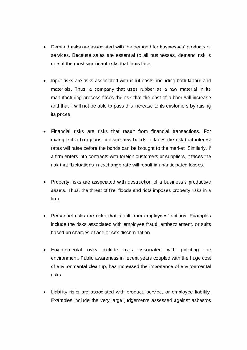
Demand risks are associated with the demand for businesses’ products or
services. Because sales are essential to all businesses, demand risk is
one of the most significant risks that firms face.
Input risks are risks associated with input costs, including both labour and
materials. Thus, a company that uses rubber as a raw material in its
manufacturing process faces the risk that the cost of rubber will increase
and that it will not be able to pass this increase to its customers by raising
its prices.
Financial risks are risks that result from financial transactions. For
example if a firm plans to issue new bonds, it faces the risk that interest
rates will raise before the bonds can be brought to the market. Similarly, if
a firm enters into contracts with foreign customers or suppliers, it faces the
risk that fluctuations in exchange rate will result in unanticipated losses.
Property risks are associated with destruction of a business’s productive
assets. Thus, the threat of fire, floods and riots imposes property risks in a
firm.
Personnel risks are risks that result from employees’ actions. Examples
include the risks associated with employee fraud, embezzlement, or suits
based on charges of age or sex discrimination.
Environmental risks include risks associated with polluting the
environment. Public awareness in recent years coupled with the huge cost
of environmental cleanup, has increased the importance of environmental
risks.
Liability risks are associated with product, service, or employee liability.
Examples include the very large judgements assessed against asbestos
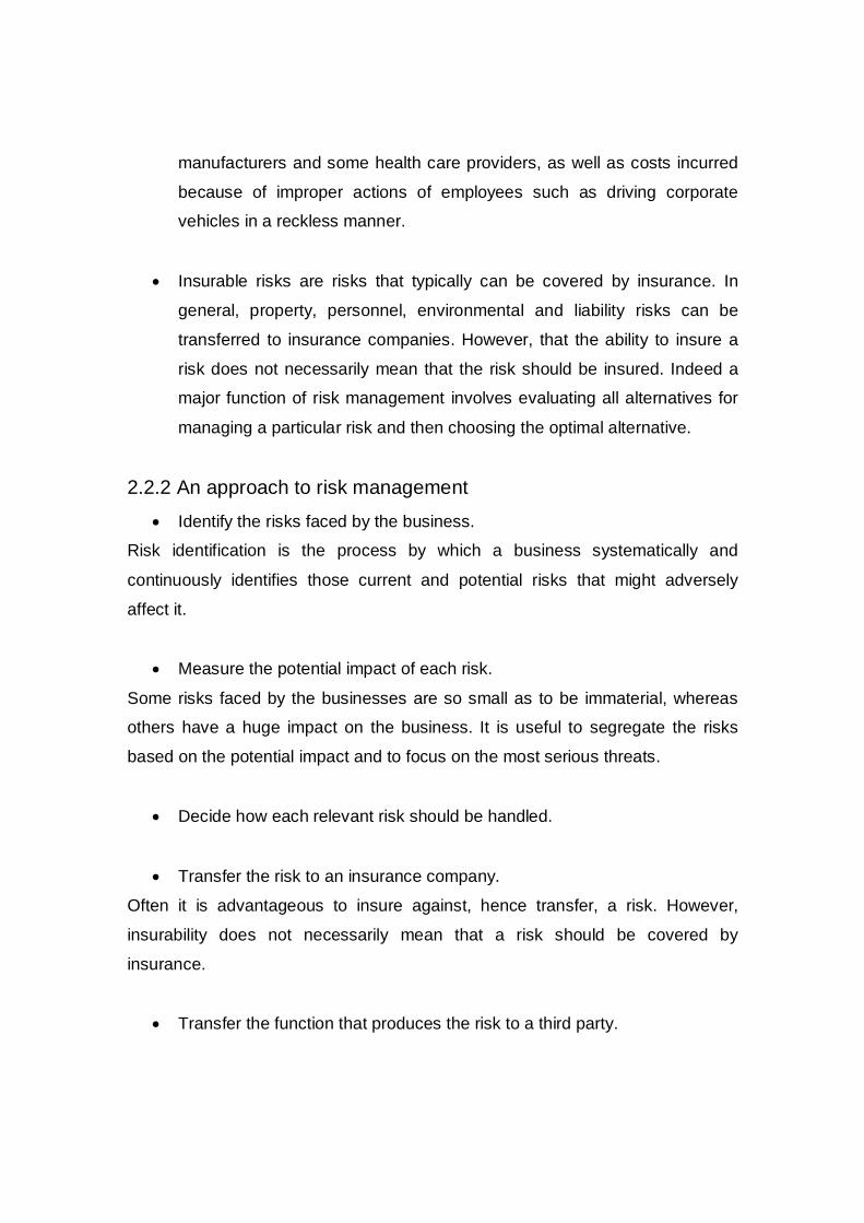
manufacturers and some health care providers, as well as costs incurred
because of improper actions of employees such as driving corporate
vehicles in a reckless manner.
Insurable risks are risks that typically can be covered by insurance. In
general, property, personnel, environmental and liability risks can be
transferred to insurance companies. However, that the ability to insure a
risk does not necessarily mean that the risk should be insured. Indeed a
major function of risk management involves evaluating all alternatives for
managing a particular risk and then choosing the optimal alternative.
2.2.2 An approach to risk management
Identify the risks faced by the business.
Risk identification is the process by which a business systematically and
continuously identifies those current and potential risks that might adversely
affect it.
Measure the potential impact of each risk.
Some risks faced by the businesses are so small as to be immaterial, whereas
others have a huge impact on the business. It is useful to segregate the risks
based on the potential impact and to focus on the most serious threats.
Decide how each relevant risk should be handled.
Transfer the risk to an insurance company.
Often it is advantageous to insure against, hence transfer, a risk. However,
insurability does not necessarily mean that a risk should be covered by
insurance.
Transfer the function that produces the risk to a third party.

In some situations, risks can be reduced most easily by passing them on to some
other company that is not an insurance company.
For example, suppose a fragile items manufacturer is concerned about potential
liabilities arising from its ownership of a fleet of trucks used to transfer products
from manufacturing plant to various distribution points across the country. One
way to eliminate this risk would be to contract with a trucking company to do the
shipping, which, in effect, passes the risks involved with transportation to a third
party.
Reduce the probability of occurrence of an adverse event.
The expected loss arising from any risk is a function of both the probability of
occurrence and the financial loss if the adverse event occurs. For example,
installing a fire prevention-training program and using fire resistant materials in
areas that have the greatest fire potential can reduce the probability that a fire
will occur.
Totally, avoid the activity that gives rise to the risk.
For example, a company might discontinue a product or service line because the
risks outweigh the rewards.
The risk management decisions like all corporate decisions should include a
rigorous cost benefit analysis for each feasible alternative.
Risk is a term that is spoken about almost casually in the financial media. Risk
and the management of risk are at the core of investment success. Without a
solid understanding of risk and the principles to mitigate it, businesses will result
in a loss.

2.3 Valuation The fundamental principle of valuation, which states that the value of any
financial asset is the cash flow, this asset generates for its owner, discounted at
the required rate of return.
2.3.1 Why is business valuation important? As the economies of the world globalise and capital becomes more mobile,
valuation is gaining importance in emerging markets for joint ventures, mergers,
acquisitions, tax, litigation, restructuring and a management tool.
One of the best reasons for obtaining a business valuation is for use as a
management tool. A prime objective for all businesses is to maximise
shareholder value. A properly prepared business valuation provides
management with insightful information, which will help them to identify company
strengths and weaknesses that affect value. A periodically prepared valuation
can serve as a measurement tool to assess management’s effectiveness and
business success.
The purpose of valuing a company is to determine a representation of the overall
worth of a business entity. The valuation of the business based on some selected
valuation techniques. The use of these methods can affect the value as well as
the information gained from the valuation process.
2.4 Valuation models Business valuation is a difficult and complex one and therefore it is a diverse
process. Valuation is more of an art than of science. Given the complexities of
analysing all factors influencing a company’s value directly, and indirectly in
combination with other factors, it is impossible to determine what a stock is worth
at a certain point in time. The best one can do to deal with this immense
complexity and to formulate a model, which is comprehensive and systematic
based on accepted valuation theory.
Valuation models, where all the future profits of the firm are specified, are called
fundamental valuation models demand much of the analyst, both concerning
knowledge about the firm’s activities and about possible developments of the
market where the firm is present. There are different fundamental valuation
models. The common factor is that the value of the stock is determined by the
present value of the future cash flows that the firm’s activities give rise to.
These valuation models are usually divided into two categories, dividend
discount models and discounted cash flow (DCF) models. The difference is that
the first discounts the dividends that the firm is expected to pay its shareholders,
while the second discounts the free cash flow that the firm’s activities are
expected to rise (Hagerud, 2000).
Three major valuation models are as follows: -
Asset based valuation.
Absolute valuation or Discounted cash flow (DCF) models
Relative valuation
There are other methods like yield-based valuation method, which focuses on
dividend yield, if the priority of investment is income or optimum valuation. This
yield-based valuation model explicitly considers management flexibility in the
value creation process.
2.5 Asset based valuation In this method, all company assets and liabilities are re-valued to a standard
value such as fair market value, fair value, intrinsic value or other representations
of standard value as a going concern. The goal of asset-based valuation is to
generate a true picture of the accounting axiom ‘assets minus liabilities equals’
owners equity.’ Appraisals of all company assets such as machinery, real estate
and intangibles are performed to the standard value.
Appraisals are also made for the company liabilities. This can be done with
analytical procedures for collective revaluation or by individually revaluing the
assets of the company. The result of this analysis is the owner’s equity that
results from the standard accounting equation.
This method may be very cumbersome in a large company, revaluing the actual
assets etc. Collective revaluation will require assumptions that may also be broad
and variable.
2.5.1 Value of assets First step is to value the assets of the company. The key considerations in
valuing various assets are discussed as follows.
Cash is cash. There is no problem in valuing it.
Generally, debtors are valued at their face value. If the quality of the debtors is
doubtful, prudence calls for making an allowance for likely bad debts.
This may be classified into three categories raw materials, work in progress and
finished goods. Raw materials may be valued at their most recent cost of
acquisition. Work in progress may be approached from the cost point of view i.e.
cost of raw materials + cost of processing. Finished goods is generally appraised
by determining the sale price realisable in the ordinary course of business less
expenses to be incurred in packaging, transporting, and selling expenses.
Current assets like deposits, prepaid expenses, and accruals are valued at their
book value.
Fixed tangible assets consist mainly of land, buildings and civil works, and plant
and machinery. Land is valued as if it is vacant and available for sale. Building
and civil work, plant, and machinery may be valued at replacement cost less
physical depreciation and deterioration. As an alternative, the value of plant and
machinery may be appraised at the market price of similar assets and cost of
transportation and installation.
Intangible assets pose a problem. As they cannot be ordinarily disassociated
from the business and sell separately, the market approach is not very helpful in
valuing them. Therefore, one may use the cost approach or the income
approach.
2.5.2 Liabilities Long – term debt, consisting of term loans and debentures, may be valued with
the help of the standard bond valuation model. This calls for computing the
present value of the principal and interest payments, using a suitable discount
rate.
Current liabilities and provisions consist of short-term borrowings from banks and
other sources, amounts due to the suppliers of goods and services bought on
credit, advance payments received, accrued expenses, provisions for taxes,
dividends, gratuity, pension etc. These are valued at face value.
The value of total ownership is simply the difference between the value of assets
and the value of liabilities.
2.6 Absolute valuation or discounted cash flow (DCF)
models The valuation of an asset is equal to the present value of all the future cash flows
that the asset will generate. The cash flows important to the stock’s value will be

dependent on the business’s future profit development, which in turn is
dependent on the sales growth and the business’s profit margin.
Discounted cash flow (DCF) analysis requires the analyst to think through the
factors that affect a business, such as future sales growth and profit margins. In
addition, it considers the discount rate, which depends on a risk-free interest rate,
the cost of capital and the risk the business faces. All of this will give an
appreciation for what drives share value. This means discounted cash flow (DCF)
analysis with appropriate and supportable data and discount rates, is one of the
accepted methodologies within the income capitalization approach to valuation.
Discounted cash flow (DCF) analysis has gained widespread application in
institutional, investment property, business valuation. This analysis is heavily
used in merger, joint ventures and acquisition situations. Discounted cash flow
(DCF) valuation models recognise that common stock represents an ownership
interest in a business and that its value must be related to the returns investors
expect to receive from holding it.
A business generates a stream of cash flow in its operations; shareholders have
a legal claim on these cash flows. The value of a stock is therefore the share of
cash flow the business generates for its owners discounted at their required rate
of return. This is the fundamental principle of valuation as developed in the
theory of investment value by John Burr Williams in 1938 (Williams, 1938).
Mathematically, the principle is expressed as follows:
n V0 = CFt / (1+k)t t=1
V0 is the value of stock in period t=0
CFt is the cash flow generated by the asset for the owner of the asset in period t
K is the discount rate.

n is the number of years over which the asset will generate cash flows to
investors.
The value of common stocks in discounted cash flow (DCF) models is
determined by the stream of expected future cash flows to investors in the
nominator and their required rate of return in the denominator. In the following,
we take a closer look at the two most widely used versions of discounted cash
flow (DCF) models:
Free cash flow discount models
Dividend discount models
The models differ only in their definition of expected cash flow to investors. As we
are valuing one specific company, we theoretically should obtain the same value
no matter which expected cash flows are discounted, as long as the assumptions
are coherent (Lundholm and O’Keefe, 2001a,b).
Obviously, a key in this method is developing the projected future earnings.
Analysts must do a thorough study of the economics of the company and the
industry must be analysed and accounted for in the analysis and projections for
the future should be made based on a detailed analysis.
In other words SWOT i.e. strengths, weaknesses, opportunities, threats, and
PEST i.e. political, environmental, and social and technical of the organisation
have to be analysed before one do the future forecast of the organisation. This
mean, the analysts who perform discounted cash flow (DCF) analysis should
exercise due diligence and best practice.
The reliability of the valuation method is depending on two factors, the reliability
of the numerator the forecast cash flow and the reliability of the denominator the
discount factor. Unfortunately, forecast values have a tendency to diverge from

the real numbers. Therefore, it is necessary to develop a reliable forecast model
in order to predict the cash flows used to value a firm.
Tax-deductible depreciation and amortization affect business’s cash flows. The
operating income should be computed after tax deductible depreciation and add
back only the tax-deductible depreciation.
For example, assume that a business has earnings before interest, tax,
depreciation and amortization EBITDA of 400 million, tax-deductible depreciation
of 100 million and non tax-deductible amortization of 50 million. Business should
use operating income of 300 million (400 less 100) to compute business’s after
tax operating income and then add back only the tax-deductible depreciation.
The projected free cash flows include factors such as a new product
development, product life cycles, competition and other value metrics associated
with company operation. An assessment of historical performance is necessary.
Short, intermediate and long-term forecasts are also necessary to develop an
adequate representation of the future economic benefits of the company, which
in turn is dependent on the sales growth and the firm’s profit margin.
Developing a reasonable forecast for the future profit development of a firm imply
extensive work. Generally, a forecast concerns the value of a variable at a
certain point in time. The purpose of forecasts and forecast models are first to
make decision-making easier and, thereby, improve the quality of the decisions
made. Analysts by organising and analysing available knowledge will be able to
decrease the uncertainty in a decision-making situation.
2.6.1 Incorporate financial and non-financial performance data Different accounting techniques can lead to different representations of a
company value. The standard procedures typically involve gathering the financial
data, manipulating it in different ways, performing the required computations and
then developing an overall representation of business value.
The asset based method and relative valuation do not address forecasting the
future to any great degree. In relative valuation, the objective is to value assets
based on how similar assets are priced in the market.
If future forecasts are made, such as with the discounted cash flow (DCF)
method, these future forecasts are based primarily on historical data. Discounted
cash flow (DCF) forecasts for the near and far term and can incorporate some
adjustments to the cash flows based on the knowledge of such things as product
introduction, machine replacements etc.
However, the method does not contain a comprehensive approach to view and
incorporate overall operational and strategic performance metrics associated with
the company. Financial forecasts based on historical financial data assume that
the future will be the same as the past, which in the ever-changing business
climate of today, may not be true.
Current financial valuation methods do not address all of the operational and
strategic perspectives associated with running a business and valuing business
activities. A more comprehensive view of overall value must be incorporated into
the valuation process. “accountants must now determine the true cost of a
company’s various business activities by establishing the value of a specific
business capability-and that includes such things as quantifying the value of
contracting out supply chain logistics or human resource management”
(Goldman 2002).
To incorporate risks into cash flows properly, start by using macroeconomic
factors to construct scenarios, because such factors affect the performance of
industries and companies in emerging markets. Then align specific scenarios for

companies and industries with those macroeconomic scenarios. The difference
here between emerging and developed markets is one of degree: in developed
markets, macroeconomic performance will be less variable. Since value in
emerging markets are often more volatile, we recommend developing several
scenarios.
The major macroeconomic variables that have to be forecast are inflation rates,
growth in the gross domestic product, foreign exchange rates, and often interest
rates. These items must be linked in a way that reflects economic realities. GDP
growth and inflation, for instance are important drivers of foreign exchange rates.
When constructing a high inflation scenario, be sure that foreign exchange rates
reflect inflation in the end, because of purchasing power parity. The theory of
purchasing power parity states that exchange rates should adjust over time so
that the prices of goods in any two countries are roughly equal.
2.6.2 Free cash flow (FCF) discount models Free cash flow is the cash that flows through a company in the course of a period
once all cash expenses have been taken out. Free cash flow represents the
actual amount of cash that a company has left from its operations that could be
used to pursue opportunities that enhance shareholder value.
Calculating free cash flow It is the remaining amount for the shareholders from revenues after deducting
operating costs, taxes, net investment and the working capital needs (WCN)
Sales revenue
-Cost of goods sold
-General and administrative expenses
…………………………………………………….
=Gross operating margin (EBDIT)
-Depreciation (*)

……………………………………………………..
=Profit before interest and taxes (EBIT)
-Income tax
……………………………………………………...
=Net profit before interest (EBI)
+Depreciation (*)
-Investment in fixed assets
-Investment in WCN (**)
……………………………………………………….
=FCF
(*) Depreciation is added back because it is a non-cash item.
(**) Working capital needs (WCN) = Cash + Receivables + Stocks - Payables
Risk premium Risk taking is inherent to a firm’s objective of shareholder wealth maximization. In
real world situation, the firm in general and its investment projects in particular
are exposed to different degrees of risk. Risk exists due to the inability of
decision makers to make perfect cash flow forecasts. This occurs because the
future events upon which they depend are uncertain.
Risk measurements in finance and economics are based on statistical measures
such as variance or its square root, the standard deviation, covariance and
correlation.
Foreign exchange risk (FOREX) There are three types of FOREX risk exposure.
Transaction exposure
Economic exposure
Accounting or translation exposure

Transaction exposure is defined as the uncertain domestic currency value
of an open position denominated in a foreign currency with respect to a
known transaction.
Economic exposure is the impact of exchange rate changes on the
uncertain foreign currency stream of corporate cash flows.
Accounting or translation exposure is caused by the uncertain domestic
value of a net accounting position denominated in a foreign currency at a
certain future date.
Therefore, developing countries as if Sri Lanka is vulnerable to currency
fluctuation and interest rates affect the success of projects significantly. One way
to avoid currency fluctuation is to arrange a forward rate agreement i.e. to say a
fixed amount of currency for a pre set price to be delivered at a known date in the
future.
Sales revenue forecast The two areas that is important when conducting a valuation,
(1) How to limit the subjectivity of the assumptions and estimations behind the
valuation
(2) How to make an accurate forecast of the future sales revenue
According to Bernstein (1996), who was referred to in the important concepts
section, forecasts are one of the most important inputs managers develop to aid
them in the decision making process. Virtually every important operation decision
depends to some extent on a forecast (Hanke, 2001). This leads to the question
of how to make accurate forecasts of future sales revenue.

Revenue forecast is the backbone of a business’s free cash flow. If the company
is keeping it busy meeting the demand, strong marketing channels and
upgraded, efficient factories the company has a reasonable competitive position,
there is enough demand for the product to maintain five years of strong growth,
but after that the market will be saturated as new competitors enter the market.
Forecasting a company’s revenues is arguably the most important and difficult
assumption analyst can make about its future cash flows. When forecasting
revenue growth, we need to consider a variety of factors. These include whether
the company’s market is expanding or contracting and how its market share is
performing. Also, need to consider whether there are any new products driving
the sales or any pricing changes are imminent. However, because that future can
never be certain, it is valuable to consider more than one possible outcome.
Sales with four Ps marketing i.e. product, price, place, promotion that comprise
the marketing mix of the firm. These ultimately determine the sales volumes. The
sales revenue-forecasting engine makes it possible for sales regional managers
to forecast potential deals in their pipeline while providing management an
accurate snapshot of the sales organisation. This powerful engine allows for in-
depth analysis of previous months, quarters and years while providing the sales
manager with the accurate data needed to forecast for future years.
Forecasting is usually easier when the firms break their sales down into
manageable parts. Not all businesses sell by units, but most do. Estimate the
sales by product line, month by month, and then add the product lines for all
months. Then convert them into value by multiplying the total number of units by
the unit sales price. It is easier to forecast by breaking things down into their
components.

Conclusion Sales forecasting will always contain elements of factual basis and judgement.
Analysts will never eliminate the judgement required. Due to this reason, we do
not have a system of programming that can create a credible sales forecast. The
balance between these two factors is the key to improving accuracy. The more
The forecast is based on facts; the more accurate is it likely to be. The facts are
drawn from:
The sales history of the company
What activities have successfully been completed with the customer for
each opportunity
What we have learned about our sales process and past forecasts to
improve our forecast process
The aim of sensitivity analysis is to discover which variables have the greatest
impact on the forecast of sales revenue. In the process of sensitivity analysis,
individual forecasted variables are progressively stepped through their
pessimistic, most likely and optimistic levels, to determine which variables cause
the largest shifts in the present value. Sensitivity analysis would be undertaken
only on the uncontrollable variables, because management would feel confident
in take control of the controllable variables.
In a world of dynamic change, all forecast variables in a project are subject to
sensitivity analysis. Due to practical constraints on time and cost, only those
variables, which could be investigated quickly and cheaply, will be investigated.
Sensitivity analysis measures the impact on business outcomes by changing the
key input values about which there is uncertainty. It is designed to identify those
variables, which have a major impact on the business’s calculated present value.
The identification of these variables should help management to refine its
forecasting function.

Cost of goods sold (cogs) / general and administrative expenses For manufacturing products the best way to calculate the cost of the product, is
to prepare the cost of the product according to the recipe of the product based on
current raw material prices in order to arrive at cost per kilogram. To arrive at the
value of the cost of goods sold, first multiply the total number of units of sales by
the weight per product to find out the total weight of sales and then multiply by
the cost per kilogram. For future years, find out the percentage of inflation rate
and increase by that percentage year on year basis.
In the same way analyst will be able to find cost of general and administrative
expenses per kilogram and multiply by the weight of the sales quantity for the
total expenses, and increase by the inflation rate year on year basis to find the
expenses for future years.
If it is not possible to find the cost per kilogram, the analyst has to look at the
company’s historic percentage of cost of goods sold (cogs) expressed as a
proportion of revenues. Analysts when forecasting have to take the side of
conservatism and assume that operating costs will show an increase as a
percentage of revenues as the company is forced to lower its prices to stay
competitive over time.
Taxation Many companies do not actually pay the official corporate tax rate on their
operating profits. For instance, companies with high capital expenditures receive
tax breaks. Therefore, it makes sense to calculate the tax rate by taking the
average annual income tax paid over the past few years divided by profits before
income tax.
Capital expenditure (CAPEX) To underpin growth, companies need to keep investing capital items such as
property, plants and equipment. Based on the company’s investment plan, the
capital expenditure can be forecasted for future years.

Change in working capital Working capital refers to the cash a business requires for day-to-day operations
or, more specifically short term financing to maintain current assets such as
inventory. The faster a business expands the more cash it will need for working
capital and investment.
Working capital is calculated as current assets minus current liabilities. Net
change in working capital is the difference in working capital levels from one year
to the next. When more cash is tied up in working capital than the previous year,
the increase in working capital is treated as a cost against free cash flow.
Working capital typically increases as sales revenues grow, so a bigger
investment of inventory and receivables will be needed to match the revenue
growth.
The entire reason we consider working capital when computing cash flows is
because investments in working capital are considered wasting assets that do
not earn a fair rate of return. Thus, money invested in inventory is wasted
because inventory sits on the shelves and does not earn a return. Short-term
debt should not be considered part of current liabilities to compute working
capital. Supplier credit, accounts payable and accrued items such as salaries,
taxes etc should be considered as part of current liabilities.

Forecast of a free cash flow: Free cash flow of ABC Ltd Rs in million Year 1 Year 2 Year 3 Year 4 Year 5 Sales revenue 100.00 120.00 144.00 172.80 207.36 Less: Cost of goods sold 50.00 59.00 69.62 82.15 96.94 Gen & administrative expenses 15.00 16.80 18.82 21.07 23.60 EBDIT 35.00 44.20 55.56 69.57 86.82 Less: Depreciation 10.00 10.00 10.00 10.00 10.00 Corporate tax 5.25 6.63 8.33 10.44 13.02 EBI 19.75 27.57 37.23 49.14 63.80 Add: Depreciation 10.00 10.00 10.00 10.00 10.00 Less: CAPEX 8.00 8.00 8.00 8.00 8.00 WCN 5.00 5.00 5.00 5.00 5.00 FCF 16.75 24.57 34.23 46.14 60.80
2.6.3 Calculating the terminal value Having estimated the free cash flow produced over the forecast period, we need
to come up with a reasonable idea of the value of the company’s cash flows after
that period i.e. when the company has settled into middle age and maturity. The
difficulty is to forecast cash flows over time. To make the task a little easier, we
use a “terminal value” approach that involves making some assumptions about
long-term cash flow growth.
Gordon growth model There are several ways to estimate a terminal value of cash flows, but one well-
known method is to value the company as a perpetuity using the Gordon growth
model. The model uses this formula:

Terminal value = Final projected year cash flow / (Discount rate – Long term cash
flow growth rate)
This formula rests on the big assumption that the cash flow of the last projected
year will stabilize and continue at the same rate forever.
TV = (FCFn) / (k-g)
Where: TV – terminal value
FCFn -- free cash flow generated by the firm in year n
n -- last year of the projections
g -- constant rate of increase in perpetual free cash flows
k -- discount rate
2.6.4 Calculating the discount rate Having projected the company’s free cash flow for the next five years, analyst
wants to figure out what these cash flows are worth today. That means coming
up with an appropriate discount rate, which we can use to calculate the present
value of the cash flows. This is a crucial decision because a difference of just one
or two percentage points in the cost of capital can make a big difference in a
company’s fair value.
A good strategy is to apply the concepts of the weighted average cost of capital
(WACC) The WACC is essentially a blend of the cost of equity and the after tax
cost of debt. Therefore, we need to look at how cost of equity and cost of debt
are calculated.
A reliable estimate of the value sensitive discount rate is essential to use in the
valuation model. Analyst’s primary goal is to gain more understanding of the

market’s perception of the risk variables associated with investing in a firm’s
stock.
Cost of equity (Ke) The cost of equity capital is equal to the required rate of return on equity-supplied
capital. The two components of a firm’s equity are equity share capital and
retained earnings. Ownership of both these funds rests with shareholders. It is
most difficult to calculate the cost of equity, because the servicing of this capital
is not a contractual liability.
Inflation is a common experience of most economies. In case of an inflationary
economy the real cost of capital is lower than the normal cost of capital. The
high rate of inflation leads to high interest rates. (Chong & Brown 2000), currency
exchange rate, interest rate directly affects the net present value or the real rate
of return on investments in projects. In addition, commodity prices are changing
rapidly.
Therefore, to cope with this difficult issue, several approaches have been
proposed:
Capital asset pricing model approach
Realised yield approach.
Bond yield and risk premium approach.
Earnings–price approach
Dividend capitalisation approach
Capital asset pricing model approach (CAPM) The most commonly accepted method for calculating cost of equity comes from
the Nobel Prize-winning capital asset pricing model (CAPM), where cost of equity
Ke = Rf + (Rm – Rf)

The CAPM was developed for measuring shareholder expectations based on the
empirical relationship of return from a particular share and that of market return.
Under the CAPM, we assume that the cost of equity is equal to the risk free rate
plus a risk premium as set forth in the security market.
Ke = Rf + (Rm-Rf)
Where: Ke - cost of equity
Rf - risk free rate
Rm - return on the market portfolio.
- systematic risk of the company
I = Cov (Ri, Rm)/m2
n _ _
Cov (Ri, Rm) = (Ri-Ri) (Rm-Rm)/n
i=1
n _
m2 = (Rm-Rm)2/n
i=1
Where: i --systematic risk of security i
Ri --return from security i.
Rm –return from market portfolio.
_
Ri -- arithmetic mean of returns from security
_
Rm -- arithmetic mean of returns from market portfolio
Where, Cov (Ri,Rm) is the covariance between the expected return of the asset
(Ri) and the expected return of the market (Rm) move together on average Ri and

Rm can be obtained from the historical data, and the covariance calculation can
be done through excel spread sheet function.
m2 is the variance of return of the market.
Capital asset pricing model (CAPM) decomposes a portfolio’s risk into systematic
and specific risk. Systematic risk is the risk of holding the market portfolio. As the
market moves, each individual asset is more or less affected. To the extent that
any asset participates in such general market moves, that asset entails
systematic risk. Specific risk is the risk, which is unique to an individual asset. It
represents the component of an asset’s return, which is uncorrelated with
general market moves.
According to capital asset pricing model (CAPM), the market place compensates
investors for taking systematic risk but not for taking specific risk. This is because
specific risk can be diversified away. When an investor holds the market portfolio,
each individual asset in that portfolio entails specific risk, but through
diversification, the investor’s net exposure is just the systematic risk of the
market portfolio.
The arbitrage-pricing model The economist Stephen Ross initiated arbitrage-pricing theory in 1976. This
theory holds that the expected return of a financial asset can be modelled as a
linear function of various macro-economic factors or theoretical market indices,
where sensitivity to changes in each factor is represented by a factor specific
beta coefficient.
The model-derived rate of return will then be used to price the asset correctly.
The asset price should equal the expected end of period price discounted at the
rate implied by model. If the price diverges, arbitrage should bring it back into

line. Under this model, a risky asset can be described as satisfying the following
relation.
E (rj) = rj + bj1 RP1 + bj2 RP2 + ……. +bjn RPn
rj = E (rj) + bJ1 F1 + bJ2 F2+ ……..+ bjn Fn + j
Where:
E (rj) is the risky asset’s expected return
rj is the risk-free rate
RPk is the risk premium of the factor
Fk is the macroeconomic factor
bJk is the sensitivity of the asset to factor k, also called factor loading
j is the risky asset’s idiosyncratic random shock with mean zero
This is the uncertain return of an asset j is a linear relationship among n factors.
Some assumptions and requirements have to be fulfilled for the latter to be
correct. The competition in the market must be perfect and the total number of
factors may never surpass the total number of assets.
Cost of debt (Kd) Compared to cost of equity, cost of debt is straightforward to calculate. The rate
applied to determine the cost of debt (Kd) should be the current market rate the
company is paying on its debt. As companies benefit from the tax deductions
available on interest paid, the net cost of the debt is actually the interest paid less
the tax savings resulting from the tax deductions interest payment. Therefore the
after tax cost of debt is Kd (1- t) where t is the corporate the tax rate.
Weighted average cost of capital (WACC) WACC is the discount rate (time value of money) used to convert expected future
cash flow into present value for all investors. Usually it is calculated by the
addition of the weighted cost of third party sources of financing and the weighted
cost of own sources of financing for their funds.
WACC = Kd (1-t)*(D/(E+D)) + Ke (E/(E+D))
Where: Kd -- cost of debt
t -- income tax rate
Ke -- cost of equity
D -- third party source of financing
E -- own source of financing
2.6.5 Country risk and cost of capital According to Roger Mills, Marcin Peksyk and Bill Weinstein, the expansion of
international trade and investment international company operations in
production, export-import and supply chain management, in the past 30 years
have stimulated interest in country risk.
The political and economic dimensions of ideological conflict surrounding
multinational companies, intensified before the collapse of Soviet Union in the
early 1990s. The demonstration of restrictive and even threatening policies
towards multinational companies on the part of newly independent nations from
the 1960s through the early 1980s, and the late 20th and early 21st centuries’
renewal of radical opposition to globalisation and international capitalism, in turn
excited the concern about the security of foreign direct investment.
Moreover, the world chessboard for foreign investment is wider than it was in the
1980s, whilst some countries remained or became no-go areas for most
investment. The expansion of opportunities included countries that have opened
to more foreign direct investment and/or that have moved into the focal range of
investors, e.g., China, South Africa, Eastern and Central Europe, India, to name
the most obvious.

In addition to this September 11, 2001 terrorist attack, invasion of Iraq and many
terrorist attacks have rejuvenated concern with the adequacy of the tools by
which risk in the field of cross-border operations and investment can be identified
and assessed-typically in uncertain conditions.
A key characteristic of the country risk analysis and ratings is that they depend
on defining categories of risk that are qualitative. The relevant evidence for
estimating such risks is predominantly qualitative. Therefore, ratings in the
numerical terms involve a relatively subjective process of conversion from
qualitative to quantitative, where the latter express some of the content of the
former (Peksyk, 2003).
The term country risk is often used when cross-border investments are
considered and which is observed and tested from the foreign investor’s
perspective. The country risk for a given country is therefore the unique risk
faced by foreign investors when investing in that specific country as compared to
the alternative of investing in other countries (Nordal, 2001). Country risk is then
the particular part of the investment’s risk, which arises from locating the
investment within specific national borders.
The early definitions of country risk stood mainly for assessing the country’s
ability to generate enough foreign exchange reserves for its external debt
obligations (Simpson, 1997). By contrast, the modern definition and its
associated calculations are more for multipurpose users like debt and equity
providers together with multinational companies when planning the engagement
in new markets.
A good example of modern definition was provided by John Ries: “country risk
relates to the likelihood that changes in the business environment will occur that
reduce the profitability of doing business in a country. These changes can
adversely affect operating profits as well as the value of assets” (Ries, 2003).

Nordal introduced a more systematic definition with an expanded methodology,
which at the end covers a wide area of modern country risk research. According
to his findings, the term country risk depends on the type of foreign investment.
The broad term can be classified into three main categories: lending, equity
investment, and foreign direct investment.
A great debate is in the academic and practitioners’ communities whether
country risk should be considered as specific risk and then dealt with by adjusting
the cash flows or as a systematic risk and expressed in the additional premium to
the discount rate.
According to Damodaran (2002), the risk premium in any equity market can be
written as:
Equity risk premium = Base premium for mature equity market + Country
premium
To calculate the base premium for a mature market, he chooses the long time to
reduce standard error, the Treasury bond to be consistent with his choice of a
risk free rate and geometric averages to reflect for a risk premium that can be
used for longer term expected returns. It is important to note that this approach
presupposes that any appraisal will be undertaken in the currency associated
with the base premium.
Once the base premium has been selected, Damodaran reviews three main
approaches for estimating the country premium, which use default risk spreads,
default spreads plus relative standard deviations and relative volatility. However,
according to Damodaran, the country risk measure captured in the default spread
is an intermediate step towards estimating the risk premium to use in risk
models.

The default spreads that come with country ratings provide an important first
step, but still only measure the premium for default risk. Intuitively Damodaran
argues that we would expect the country's equity risk premium to be larger than
the country default risk spread. To address the issue of how much higher, he
uses the volatility of the equity market in a country relative to the volatility of the
country bond, used to estimate the spread.
Country equity risk premium = Country default spread x (Standard deviation
Equity/Standard deviation country bond)
Godfrey and Espinosa (1996) found that:
All developed countries have betas higher than 0.5.
Fifteen out of the 26 emerging market countries have betas below 0.5.
Four such countries have negative betas, implying costs of equity below risk free
rates.
Risk premium in emerging market countries is lower than the risk premium for the
US.
By comparison, Godfrey and Espinosa found that the volatility of the emerging
markets from the analysis is measured by the standard deviation of mean equity
returns revealed a picture far more in keeping with expectations. According to
this approach adjustments to the risk free rate are made for country risk by the
addition of a credit spread, and to the beta for the volatility of the market in
relation to a US reference point, as measured by the relative standard deviation,
i.e.,
Ke = (Rfus + country default spread) + (adjusted *ERPus*)
Where:
Ke = Estimated cost of equity
ERPus = US market risk premium
Rf = Risk free rate

Adjusted = (i / us ) i.e., the standard deviation of stock market returns in the
country of the prospective investment divided by the standard deviation of the US
stock market.
= Adjustment for the interdependence between the risk free rate and the
market risk premium
Damodaran reviews all the three approaches and argues a case for the second
as being a favourite one because the larger risk premiums result are the most
realistic for the intermediate future. He also recognises that country risk
premiums will decline over the time such that as companies mature and become
less risky over time; countries can mature and become less risky as well. This
has been confirmed by Gangemi in1999 who examined the 25-year period from
1970 to 1994 consisting of monthly data on 18 countries drawn from the Morgan
Stanley database.
While assessing the country risk is a challenge, there is yet another problem in
terms of evaluating how individual companies in that country are exposed to
country risk. Damodaran used three alternative approaches to evaluate the
country risk to a Polish quoted company.
Assume that all companies in a country are equally exposed to country risk.
Thus, for Poland, with its estimated country ERP of 7.52%, each company in the
market will have an additional country risk premium of 2.99% added to its
expected returns. For instance, the cost of equity for the company listed in
Poland, with a beta of 0.89, in GBP terms would be 12.22% assuming a UK Gilt
rate of 5.20% and a mature market UK risk premium of 4.53%.
Expected cost of equity = 5.20% + 0.89 (4.53%) + 2.99% = 12.22%
Damodaran recognises that the biggest limitation of this approach is that it
assumes all firms in a country, no matter what their business or size, are equally
exposed to country risk.
Assume that a company’s exposure to country risk is proportional to its exposure
to all other market risk, which is measured by the beta. For Poland Company,
this would lead to a cost of equity estimate of:
Expected cost of equity = 5.20% + 0.89 (4.53% + 2.99%) = 11.89%
Allow each company to have an exposure to country risk that is different from its
exposure to all other market risk as follows:
Expected return = Rf + β (mature equity risk premium + k (country risk premium)
Using this rationale, Poland company, which derives 23% of its revenues in the
global market in foreign currencies, should be fairly exposed to country risk.
Using a k of 0.77, resulting cost of equity in GBP terms for Poland company
Expected return = 5.20% + 0.89(4.53%) + 0.77(2.99%) = 11.53%
Three different expected returns are the result of applying three different
approaches. The higher the percentage, the greater is the assessment of country
risk and the lower would be the resulting net present value in a discounted cash
flow analysis.
Two types of parallel analysis was undertaken, version 1 used scenario analysis
weighted with the probability and version 2 shows similar results by adjusting the
discount rate for country risk.

Measuring country risk is an important challenge. Research must involve a range
of diverse examples, both as to countries and types of project, in which various
iterations are found for the alignment of cash flows with the impacts derived from
scenarios whose content is typically stated in qualitative terms. In other words,
there must be rigorous cross checking and adjustment between qualitative and
quantitative analysis.
Like the earliest stages of a scientific development, the models we have explored
are revealed on close examination to achieve no more than to point in a general
direction of solutions and are they unable to provide answers. In the area of
country risk, notably focused on the accession countries, it is important that less
ambiguous techniques should be developed.
The quest is for the development of a model, which is not as presumptuous as to
produce an answer but to provide a sound basis for interrogating the quality of
the assumptions made.
2.6.6 Calculating total enterprise value (EV) To arrive at a total enterprise value (EV), we simply have to take the present
value of the cash flows and terminal value, divide them by the discount rate and
finally add up the results.
EV = FCF1 / (1+WACC)1 + FCF2 / (1+WACC)2+ …… + FCFn / (1+WACC)n + TV
/ (1+WACC)n
Where: EV is enterprise value
FCF is free cash flow of the enterprise
WACC is weighted average cost of capital
n is the number of years
TV is the terminal value

2.6.7 Calculating the value of equity (Ve) Enterprise value includes the company’s debt. Investors are interested in the
value of the enterprise’s shares alone. The value of the enterprise’s equity is
equal to enterprise value less net debt of that enterprise.
EV = Ve + Vd Ve = EV – Vd
Where: Ve is the value of equity
Vd is the value of debt
EV is the enterprise value.
2.6.8 How do the analysts value a business that is losing money? Businesses that are losing money currently create several problems for the
analysts who are attempting to value them. There are number of reasons why a
business might have negative earnings, and the response will vary depending
upon the reason:
If the earnings of a cyclical firm are depressed due to a recession, the best
response is to normalise earnings by taking the average earnings over an entire
business cycle. A good example would be Ford or Chrysler in 1991, when both
companies had negative earnings because of the recession.
Normalised net income = Average ROE * Current book value of equity
Normalised after tax operating income = Average ROC * Current book value of
assets
Once earnings are normalised, the growth rate used should be consistent with
the normalised earnings, and should reflect the real growth potential of the firm
rather than the cyclical effects.
If the earnings of a firm are depressed due to a one-time charge, the best
response is to estimate the earnings without the one-time charge and value the
firm based upon these earnings. For example, it would apply to firms that had
significant restructuring charges.
If the earnings of a firm are depressed due to poor management, i.e. the firm is a
poor performer in a sector with healthy earnings; the average return on equity or
capital for the industry can be used to estimate normalised earnings for the firm.
The implicit assumption is that the firm will recover back to industry averages,
once management has been removed.
Normalised net income = Industry average ROE * Current book value of equity
Normalised after tax operating income = Industry average ROC * Current book
value of assets
If the negative earnings over time have caused the book value to decline
significantly over time, use the average operating or profit margins for the
industry in conjunction with revenues to arrive at normalised earnings. Note that
in the context of a discounted cash flow valuation, this normalisation will occur
over time rather than instantaneously.
Thus, a firm with negative operating income today could be assumed to converge
on the normalised earnings five years from now. (This would be the approach to
use for a firm like Digital Equipment, which had low earnings in 1996, while other
firms in the sector were reporting record profits)
If the earnings of a firm are depressed or negative because it operates in a
sector, which is in its early stages of its life cycle, the discounted cash flow
valuation will be driven by, the perception of what the operating margins and
return on equity (ROE) will be when the sector get matured. (This would apply for
firms in the cellular technology business in the mid nineties.)

If the equity earnings are depressed due to high leverage, the best solution is to
value the firm rather than just the equity, factoring in the reduction in leverage
over time. (This would be the choice when valuing a firm right after a leveraged
buyout.)
2.6.9 Pros and cons of discounted cash flow DCF We have gone through the mechanics of discounted cash flow analysis, now it is
worth to examine the method’s strengths and weaknesses.
The best reason is that it produces the closest value to an intrinsic stock value.
The alternatives to discounted cash flow (DCF) are relative valuation measures,
which use multiples to compare stocks within a sector. While relative valuation
metrics such as price earnings (P/E), enterprise value to earnings before interest,
tax, depreciation and amortization (EV/EBITDA) and price to sales ratios are
simple to calculate, they are not very useful if an entire sector or market is over
or undervalued. A carefully designed discounted cash flow (DCF) can be used as
a management tool to grab the opportunities in order to maximise the
shareholder value and to reduce the threats to the company.
Unlike standard valuation tools such as the P/E ratio, discounted cash flow (DCF)
relies on free cash flows. Free cash flow is a trustworthy measure that avoids
much of the arbitrariness involved in reported earnings.
Although discounted cash flow (DCF) analysis certainly has its merits, it also has
its share of shortcomings. If the inputs free cash flow forecasts, discount rates
and perpetuity growth rates are not correct due to uncertainties; the value
generated for the company will not be accurate.
Discounted cash flow (DCF) analysis is dynamic in nature; it demands constant
vigilance and modification. The model is not suited to short term investing; it
focuses on long-term value. A well-crafted discounted cash flow (DCF) may help

you avoid buying a bubble, but it may also make you miss short-term share price
run-ups that can be profitable.
2.6.10 Summary Discounted cash flow (DCF) analysis tries to work out the value of a company
today based on projections of how much money it will generate in the future. The
basic idea is that the value of any company is the sum of cash flows that it
produces in the future, discounted to the present at an appropriate rate.
Discounted cash flow (DCF) analysis treats a company as a business rather than
just a stock price, and it requires you to think through all the factors that will affect
the company’s performance. What DCF analysis really gives you is an
appreciation for what drives stock values.
2.7 Discounted dividend model In economic terms, the intrinsic value of a share must be equal to the present
value of the expected flow of all future cash payments to an investor, including
dividend payments as well as the proceeds from the final sale of the share. The
dividend discount model (DDM) is the theoretically most correct model for firm
valuation (Miller and Modigliani, 1961).
The market price is determined by the dividends the new owner of the security
expects to receive over his holding period. From this follows that the market price
can be replaced again by a stream of dividends, until the entire value of the stock
is expressed in terms of dividends.
V0 = D1 /(1+k) + D2 /(1+k)2 +…..+Dt /(1+k)t + Pt /(1+k)t with
Pt = Dt+1 /(1+k)t+1 + Dt+2 /(1+k)t+2 +…..+ Dn / (1+k)n
n becomes V0 = Dt /(1+k)t 1-1 t=1
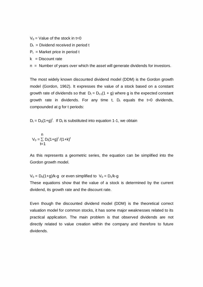
V0 = Value of the stock in t=0
Dt = Dividend received in period t
Pt = Market price in period t
k = Discount rate
n = Number of years over which the asset will generate dividends for investors.
The most widely known discounted dividend model (DDM) is the Gordon growth
model (Gordon, 1962). It expresses the value of a stock based on a constant
growth rate of dividends so that Dt = Dt-1(1 + g) where g is the expected constant
growth rate in dividends. For any time t, Dt equals the t=0 dividends,
compounded at g for t periods:
Dt = D0(1+g)t. If Dt is substituted into equation 1-1, we obtain
n V0 = Dt(1+g)t /(1+k)t t=1
As this represents a geometric series, the equation can be simplified into the
Gordon growth model.
V0 = D0(1+g)/k-g or even simplified to V0 = D1/k-g
These equations show that the value of a stock is determined by the current
dividend, its growth rate and the discount rate.
Even though the discounted dividend model (DDM) is the theoretical correct
valuation model for common stocks, it has some major weaknesses related to its
practical application. The main problem is that observed dividends are not
directly related to value creation within the company and therefore to future
dividends.
According to Miller and Modigliani, (1961) currently observed dividends are
inaccurate unless the payout policy is tied to the value generation within the
company. Penman (1992) describes: “”price is based on future dividends but
observed dividends do not tell us anything about price.”” The missing link
between value creation and value distribution leads to a problem in forecasting
dividends, as it is difficult to forecast payout ratios.
According to Professor T.E. Copeland, the first thing is to understand that the
discounted cash flow valuation method is an entity or an enterprise approach
where the cash flows from all sources of capital are valued and then one
subtracts the value of debt to get the value of equity.
The dividend discount model is an approach that is very similar to discounted
cash flow (DCF). What it does is it takes the free cash flows to the shareholders,
discounts them at the cost of equity and in fact one gets the same answer as with
the enterprise approach.
An important additional consideration, which is that both the discounted cash flow
method and the dividend method are used to forecast the future cash flows, while
the intrinsic value method uses historical information. Taking the book value of
equity as an example, this has little to do with the market value of the equity and
the ratio of market value to book value is rarely equal to one.
In fact, many companies that have negative intrinsic value, if one are using the
book value of equity as a measure. Book value is therefore not highly correlated
with the market value of the enterprise or the market value of equity.
2.8 Relative valuation 2.8.1 First principles: In discounted cash flow (DCF) valuation, the objective is to find the value of an
asset, given its cash flow, growth and risk characteristics. In relative valuation,

the objective is to value an asset, based upon how similar assets are currently
priced by the market. Consequently, there are two components to relative
valuation.
The first is that to value assets on a relative basis, prices have to be
standardized, usually by converting prices into multiples of earnings, book values
or sales. The second, similar firms have to be found to compare the standardized
multiples in order to determine their relative adequacy.
In the context of valuing equity in firms, the problem is the firms in same business
can still differ on risk, growth potential and cash flows. The question of how to
control for these differences, when comparing a multiple across several firms,
becomes a key one. While relative valuation is easy to use and intuitive, it is also
easy to misuse.
Four main methods using different multiples are commonly used in the relative
approach to valuation.
Relative earnings valuation method: P/E ratio or earnings multiple, PEG
ratio
P/E = Price/Earnings per share
PEG = P/E/g, where g is the expected growth rate of earnings.
Relative revenue valuation method: P/S ratio
P/S = Price/ Sales per share.
Relative cash flow valuation method. P/EBIT, P/EBITDA, P/CFO ratios
Where EBIT is earnings before interest and tax
EBITDA earnings before interest, tax, depreciation and
amortization
CFO cash flow from operation.
Earnings multiples are commonly used when analysts have high confidence in
the quality of historical and projected earnings per share (EPS) and when

earnings per share (EPS) are expected to grow. The revenue based valuation
method is used when earnings are negative or declining or when earning figures
are not comparable or not representative for the future. Cash flow ratios are used
in industries, which have low or negative earnings per share (EPS) due to large
non-operating expenses or for cyclical companies with high earnings volatility.
2.8.2 What is relative valuation? In relative valuation, we value an asset based upon how similar assets are priced
in the market. There are three essential steps in relative valuation. The first step
is finding comparable assets that are priced by the market. Analysts use other
companies in the same sector as comparable, but the question is whether this
practice really yields similar companies.
The second step is scaling the market prices to a common variable to generate
standardized prices that are comparable. This equalisation requires converting
the market value of equity or the firms into multiples of earnings, book value or
revenues.
The third and last step in the process is adjusting for differences across assets
when comparing their standardized values. Many analysts adjust for these
differences qualitatively, making every relative valuation a story telling
experience.
2.8.3 Reasons for popularity Why is the use of relative valuation so widespread? Why do managers and
analysts relate so much better to a value based upon a multiple and comparables
than to discounted cash flow (DCF) valuation? The reasons behind the popularity
of multiples are as follows.
It is less time and resource intensive than discounted cash flow (DCF) valuation.
Discounted cash flow (DCF) valuation requires substantially more information

than relative valuation. Analysts who are faced with time constraints and limited
access to information; relative valuation offers a less time intensive alternative.
It is easy to defend discounted cash flow (DCF) valuation with their long lists of
explicit forecasts and workings of discount rate is much more difficult to defend
than relative valuations, where the value used for a multiple often comes from
what the market is paying for similar firms.
Relative valuation is much more likely to reflect the current mood of the market,
since it attempts to measure relative and not intrinsic value. This is important for
the investors who make judgements on relative value.
2.8.4 Potential pitfalls The strengths of relative valuations are also its weaknesses. A relative valuation
can be put together, pulling together a multiple and a group of comparable
businesses, can also result in inconsistent estimates of value where key
variables such as risk, growth or cash flow potential are ignored.
The fact that multiples reflect the market situation also implies that using relative
valuation to estimate the value of an asset can result in values that are too high,
when the market is over valuing comparable businesses, or too low, when it is
under valuing these businesses. The lack of transparency of the assumptions in
relative valuations makes the valuation vulnerable to manipulation.
2.9 Reconciling relative and discounted cash flow valuations The two approaches to valuation, discounted cash flow valuation and relative
valuation will generally produce different estimates of value for the same
business. Furthermore, even within relative valuation, you can arrive at different
estimates of value, depending upon which multiple you use and what businesses
you based the relative valuation on.

The differences in value between discounted cash flow valuation and relative
valuation come from different views of market efficiency, or market inefficiency.
There is a significant philosophical difference between discounted cash flow
(DCF) and relative valuation.
In discounted cash flow (DCF) valuation, we are attempting to estimate the
intrinsic value of an asset based upon its capacity to generate cash flows in the
future. In relative valuation, we are making a judgement on how much an asset is
worth by looking at what the market is paying for similar assets.
In relative valuation, we estimate the value of an asset by looking at how similar
assets are priced. To make this comparison, we begin by converting prices into
multiples standardizing prices and then comparing these multiples across
businesses that we define as comparable. Prices can be standardized based
upon earnings, book value, and revenue or sector specific variables.
Chapter 3 Methodology
3.0 Method approaches Considering the approach to problem is a very vital aspect. This section
discusses the choice between inductive and deductive approach, qualitative and
quantitative approach, and, finally, a description of how the approach of this
thesis was developed.
3.1 Inductive or deductive approach Two approaches are available namely, the inductive approach and the
hypothetical deductive approach (Halvorsen, 2001). The inductive approach
involves the practice of having no clearly defined hypotheses and a vague
problem definition. In general, this type of approach is used in social sciences
studies due to its unpredictability. The hypothetical deductive approach, on the
other hand, involves judging the tenability of a hypothesis through essential
testing of it. This approach is more suitable for studies which will use quantitative
data and will reach a conclusive answer, such as “either of” results.
3.2 Quantitative and qualitative approach Statistical methods can be used to solve problems of a quantitative kind
(Halvorsen, 2001). When using the quantitative approach it is most common to
use standardised interviews or questionnaires. The reason is that when using
this method, it is common to have a good idea of what phenomenon the study is
trying to investigate and asking appropriate questions could lead the study in the
right direction.
Qualitative methods can preferably be used when the study is of a more
exploring kind (Halvorsen, 2001). Examples of such methods are observations
and unstructured interviews. Qualitative methods are more suited for studies of
occurrences that cannot be measured such as those common in social sciences
studies.
3.3 Research approach The methodology employed in this research also entailed a combination of
questionnaire, personal interview and library and desk research. The researcher
constructed a questionnaire consists of three parts, part I is about the details of
the businesses, part II about the valuation techniques and what methods they
adapt to calculate the inputs for their valuation techniques and part III open
questions about the problems and limitations of these methods.
Questioning why DCF is a better valuation technique compared with asset based
and valuation of businesses is a quantitative, qualitative and deductive in nature.
Its purpose is exploratory inviting the researcher to look for characteristics.
3.4 Research design The focus of the research study was to test the hypothesis that businesses,
shareholders and investors rely on different types of valuation techniques to
maximise the accuracy of these techniques.
This research is based on five steps.
Closer familiarisation of researcher with valuation techniques of businesses,
which is based on a literature review
Pilot survey in order to ascertain and detect any ambiguities, questions that
are not easily understood or poorly constructed and even those that are
irrelevant to the respondents
Several interviews to get more comfortable in respect to its application of
valuation techniques
Interviews –face to face personally administered questionnaires
Optionally one or more additional interviews to retrieve more detailed
information regarding distressed and hi-tech projects

3.5 Data collection methods 3.5.1 Sample The sample population of this study consists of sixty-three representatives of
manufacturing businesses in Sri Lanka. These representatives were CFOs,
Senior Financial Managers, accountants and financial analysts. The key criterion
for their selection was that the participants must play an integral role in their
companies’ strategies for valuation of their businesses.
A pilot survey was conducted in order to ascertain and detect any ambiguities,
questions that were not easily understood or poorly constructed and even those
that were irrelevant to the respondents.
From the responses, remarks and comments received on the pilot survey, the
entire questionnaire was refined and improved upon to take care of the observed
shortcomings, enhance the validity, and make the questions easier to answer
and more response friendly.
From the pilot survey, desk research and discussions with analysts of the
businesses the researcher discovered that there were problems and challenges
in forecasting accurate free cash flows of the businesses.
3.6 Modes of data collection The researcher had used two widely used methods for collection of primary data
by mailing questionnaires and personal interviews. Each method has its
advantages and disadvantages. In general, personal interviews and telephone
surveys elicit much higher rate of response than mailed questionnaires.
With the face-to-face interview, there is interaction between the interviewers and
the interviewee and can guide the respondent through a series of questions. A

higher response is achieved by this method. Questionnaires the most important
of these the target questions about the central topic of the study.
Researcher deliberately kept the number of questions as low as possible to avoid
discouragement of those willing to participate.
3.6.1 Advantages of questionnaire Questionnaires are cost effective and easy to analyse. Questionnaires are
familiar to most people and reduce bias. Questionnaires are less intrusive than
telephone or face-to-face surveys. When a respondent receives a questionnaire
in the mail, he is free to complete the questionnaire on his own timetable. Unlike
other research methods, the research instrument does not interrupt the
respondent.
3.6.2 Disadvantages of questionnaire One major disadvantage of written questionnaire is the possibility of low
response rates. Another disadvantage is the inability to probe responses.
Questionnaires are structured instrument; allow only little flexibility to the
respondent with respect to response format. By allowing frequent space for
comments, the researcher can partially overcome this disadvantage. Comments
are among the most helpful of all the information on the questionnaire, and they
usually provide insightful information that would have otherwise been lost.
3.7 Deductive approach Secondary data was collected from textbooks borrowed from British Council
library and Public library and from Journal articles and research articles was
collected from World Wide Web sites.

The piloting of the questionnaires proved very useful in the constructing of a
comprehensive, easy to understand and respond to final version that was used in
the research.
In order to collect primary data, an abstract of the semi-structured questions was
sent to the interviewees, together with a brief letter explaining the purpose of the
interview. The context of the interview was therefore clear resulting in an
effective usage of the one-hour scheduled for each interview. Mostly the
researcher had an interview with the chief financial officers, financial analysts
and accountants and in some cases the senior managers. In few instances
researcher had the opportunity to interview the foreign investors, armed with the
final version of the survey the level of self-confidence increased regarding the
subject. They were very corroborative and spent their valuable time with the
researcher to answer the questions.
Questionnaire was designed to gather information about the type of the
business, finally asked for any constraints and shortcomings experienced during
the valuation process.
The unrestricted questions in the questionnaire provided many opportunities for
respondents who wished to elaborate or write at length on some pertinent issues
relating to the business.
The respondents were given tailor made introductory explanations and not more
than necessary during data collection process, this explanation stimulated the
respondents’ interest on the research topic. The researcher assured that the data
about respondents’ businesses would be kept confidential. Too much information
can introduce bias, but some respondents demanded more detail.
Researcher had explained to the respondents the objective of the study, and its
background. In addition, the researcher explained how the selections of the
respondents were made and the benefits could derive from the research. When
the researcher went to interview, some of the respondents were busy so the
researcher had to give a general introduction and tried to stimulate enough
interest and managed to arrange an interview at another time.
The personal interviews represented excellent media for close interaction and
rapport between the researcher and the respondents, which enabled the former
to elicit information that is more pertinent and data, which the questionnaire
neither captured nor provided for. The personal interviews in addition provided
the researcher the flexibility to cater for and appreciate the peculiarities and
uniqueness of some of the respondents, through asking them pertinent questions
and listening to their own perspectives and views on the subject. The primary
data for this study were thus collected using the questionnaires and personal
interviews.
The combination of the questionnaire and personal interviews complemented by
desk research significantly contributed in ensuring that the researcher got to the
root of the challenges and shortcomings of the valuation techniques.
The successful interview is based on rapport meaning a relationship of
confidence and understanding between interviewer and respondent.
A difficult task in interviewing is to make certain the answers adequately satisfy
the question’s objectives. It is important to have this information well in mind
because many first responses are inadequate even in the best-planned studies.
The technique of stimulating respondents to answer more fully and relevantly is
termed probing, since it presents a great potential for bias during the interview, a
probe was made as neutral and as a natural part of the conversation. Appropriate
probes were used without eliciting the desired information. Responses were
recorded, as they occur in order to avoid the chance of losing any information.
Abbreviations of words, especially key words were recorded since the time factor
was a constraint during the interview.
3.8 After the interviews, the following steps were taken: A summary sheet was compiled with a list of all written responses to the
Questions
Notes were created about links to literature, emerging patterns.
Data was reduced to meaningful and manageable amounts.
Data was reduced but accounted for all data.
The data was grouped and classified.
An analytical framework was identified with the help of classified data.
Finally, statistical techniques were used in the analysis.
3.9 Reliability and validity of the data To cater to the concerns of reliability and validity of the study, two types of
research methods were used that collected both quantitative and qualitative data.
By using a multi-method research approach, the limitations and biases of one
method were compensated by the others. For example, while the questionnaires
provide objective information about the valuation of the businesses, they do not
reveal the underlying motives of the policies. Through the interviews, the
participants were asked about the rationale behind these valuation techniques.
Moreover, the possibilities of bias were highly alerted by eliciting the perspectives
of the respondents during the interviews without imposing their perspectives on
them. The use of follow up interviews and the provision of transcripts of the
interviews to the respondents for modifications of errors minimise the impact of
the biases.
Finally, discrepancies or negative cases were paid attention. These cases were
analysed closely in order to determine how and why they affect the interpretation
of data results.
3.10 Statement of hypothesis The null hypothesis H0 states that the different techniques of valuation of
businesses will produce the same results.
The alternate hypothesis H1 assumes that the different techniques of valuation of
businesses will not produce the same results.
3.11 Statistical techniques used in the analysis The statistical techniques used in the analysis of the data for this research
include frequency distribution, the correlation and Pearson chi-square.
The chi-square test statistic and the distribution of means were used in the
testing of the hypotheses. The justification for the use of chi-square distribution
with k-1 degrees of freedom, where k is the number of categories is driven by the
fact that the responses fall into categorical data.
3.12 Summary In this chapter, the research design selected for this study was presented. Each
of the methods—questionnaires and interviews—that were used to collect and
analyse the data was discussed. The chapter also set out the data collection and
data analysis procedures. The data collection process involved conducting
interviews and questionnaires to obtain primary data. Finally, the methods of
resolving reliability and validity concerns of the dissertation were briefly
discussed.
Chapter 4 Results and discussion
4.0 Introduction In this chapter, the findings derived from the research of 63 businesses in Sri
Lanka were presented. The research reveals the valuation techniques and the
pros and cons of those and the inputs of the valuation technique in discounted
cash flow (DCF) technique. The methods used to calculate the inputs and the
problems and limitations of those methods.
Moreover, the information obtained from the semi-structured interview with the
chief financial officers (CFOs), financial analysts, accountants and financial
managers offer detailed explanations about the valuation techniques used and
how they use as a management tool in their businesses.
4.1 Descriptions of participants The sixty-three participants of this study included: chief financial officers,
financial managers, financial accountants, and financial analysts from different
types of businesses as shown in Table 1.
The 63 participants under the research study have an issued share capital as
shown in Table 2. Their average annual turnover for the last three years was
shown in Table 3. The number of employees of the businesses was shown in
Table 4.
4.2 Participants’ views The participants are highly experienced and well educated. Thus, they should be
able to provide valuable insights into business valuation techniques.
4.2.1 Valuation techniques About 82.5% of respondents were of the opinion that discounted cash flow (DCF)
valuation technique is better than the other valuation techniques. They were of
the opinion that discounted cash flow (DCF) valuation technique counts its
valuation on future free cash flows, in reality; the investor or the shareholder
receives the future free cash flows from his investment. Discounted cash flow
(DCF) valuation technique acts as a management tool and helps them in the
effective management of their businesses.
In addition, they were of the opinion that the forecast of free cash flows is the
backbone of discounted cash flow (DCF) valuation technique. If the free cash
flows generated from the business were not sufficient to satisfy the shareholder
wealth maximisation, the management immediately can act with due-diligence in
order to find out the weaknesses and threats to the business in future and can
apply their core competences in order to remedy the situation.
Some respondents were commented that the reason to use discounted cash flow
(DCF) valuation technique is that it produces value closest to intrinsic stock
value. The alternatives to discounted cash flow (DCF) valuation technique are
relative valuation measures, which use multiples to compare stocks within a
sector. While relative valuation metrics such as price earnings (P/E), enterprise
value per earnings before interest, tax, depreciation and amortization
(EV/EBITDA) and price to sales ratios are simple to calculate, they are not very
useful if an entire sector or market is over or undervalued.
Unlike standard valuation tools such as the price earnings (P/E) ratio, discounted
cash flow (DCF) valuation technique relies on free cash flows. For the most part,
free cash flow is a trustworthy measure that cuts through much of the
arbitrariness involved in reported earnings.

The balance 17.5% of the respondents was of the opinion that discounted cash
flow (DCF) valuation technique works best when there is a high degree of
confidence about future cash flows. However, things can get tricky when a
business’s operations lack what analysts call ‘visibility’, that is when it is difficult
to predict sales and cost trends with much certainty. While forecasting cash flows
a few years into the future are nearly impossible. Therefore, discounted cash flow
(DCF) valuation technique is susceptible to error.
Some respondents were of the view for the starting business; the discounted
cash flow (DCF) valuation technique is only as good as its input assumptions.
Depending on what the analysts believe about how a business will operate and
how the market will unfold, discounted cash flow (DCF) valuations can fluctuate
wildly. If the inputs free cash flow forecasts, discount rates and perpetuity growth
rates are wide of the mark; the fair value generated for the business would not be
accurate.
4.2.2 SWOT analysis Eighty two percent (82%) of the respondents were commented that they perform
a fundamental analysis of their business before do the estimate of future free
cash flow. This analysis is to find the strengths and weaknesses of the business's
operations and to relate these to the business value. They do this analysis with a
combination of strategic analysis and a financial analysis.
The strategic analysis aims at understanding the opportunities and threats the
business faces or will face in the future and take into account. The financial
analysis is based on historical figures of earlier performance. These figures will
then be extended into the future to determine the expected free cash flow.
They were of the opinion that it is impossible to conduct a good financial analysis
without strategic analysis. Since the historical cash flows have to be understood
in the light of the historical competitive environment, and future changes in that

environment is what will cause changes in future free cash flows. The financial
analysis should result in acquiring knowledge of the key success factors that
affect the future free cash flows and how to measure the key success factors and
their potential changes.
Furthermore, some of the respondents brought to attention that the business’s
future performance should be based on a through strategic analysis of the
business and its industry. This result in finding out what drives the company’s
value is whether and how long a business can earn returns in excess of its
opportunity cost of capital. In order to achieve this they make use of competitive
advantage, since the lack of competitive advantage would force all the
companies in the industry to earn no more than their cost of capital.
4.2.3 Financial forecasts Eighty two percent (82%) of the respondents were commented they translate the
strategic analysis into a financial forecast through a process of financial analysis.
Then they go to the next step and create the financial forecast for the valuation
process.
Since sales affect the size of all other financial variables, the financial teams of
the respondents’ businesses takes due care in forecasting future sales and this is
the key starting point for financial models. In addition to predicting sales, and
some of the businesses do sensitivity analysis, simulation in order to avoid
mistakes in large magnitude.
According to some of the respondents, that their sales forecast based on internal
and external analysis. The problems they face with an internal analysis
performed by their managers is that they tend to overlook significant trends in the
economy and within the industry. They use regression analysis to estimate the
relationship between industry sales and the economy in general. Their sales

forecast involve with information about their business, macroeconomic trends,
the market etc in order to be as accurate as possible.
Some of the respondents were of the opinion that the information needed to
forecast the best possible manner are the business specific information,
macroeconomic information that have an impact on the sales, information about
competitors on future prospects, private information about their business.
According to the respondents, first they concentrate in finding the determinant of
sales in order to forecast the sales figure of their businesses. They mentioned
two main areas of independent variables, general indicators GDP, inflation and
industry and business specific indicators, such as price index.
In addition, they were of the opinion, since there are many more factors, which
can affect sales; it is more difficult to define the independent variables. Normally
they create an economic model over the environment of the business in order to
prepare a tool to find the determinants of sales but they said this of-course
incomplete but this tool helps the analysts to make decisions on the factors that
affect the outcome of sales and to try to take control of those.
According to 33% of the respondents, they use time series analysis such as
moving average, exponential smoothing to forecast the sales revenue of their
businesses. They use the company’s historical sales data, discover the pattern
involved in the past and then forecast the company's future sales.
The forecaster usually performs four types of analysis trend, cycle seasonal and
random factor. They said time series analysis is an effective forecasting method
in situations where the historical pattern will continue in the future but this does
not take into account what is expected to happen in the economy and in the
company’s industry.
Another 62% of the respondents said they use causal forecasting technique such
as econometric forecasting (regression models) to forecast sales revenue. Since
causal forecasting technique considers a number of variables that are related to
the variable, which is going to be predicted, this model is more powerful than the
time series methods.
Regression analysis determines which variables are important indicators. The
correlation between two variables gives a good estimate. In the case of time
series analysis, these methods are concerned with past sales and the fact that
the future sales in some way reflect the past sales numbers. If the past data is
exhibiting a constant rise in the sales, consequently the sales forecast show an
increase even if the business cycle is declining.
The other 5% of the participants said that they use qualitative methods such as
customer survey, sales force composites and Delphi method in forecasting their
businesses’ sales revenue. According to them, these techniques provide a
reasonably good forecast as long as a knowledgeable expert does this.
Some of the participants mentioned that two items most directly contradict the
definition of operating income are operating leases and research and
development (R&D) expenses, both of which are categorized as operating
expenses. Operating leases are financial expenses and research and
development (R&D) expenses are capital expenses.
4.2.4 Terminal value Fifty nine percent (59%) of the participants use stable growth model to calculate
the terminal value. Another 6% use multiple approaches to calculate their firms’
terminal value but even the 59% who use stable growth model use multiple
approach method as well to check the accuracy of their value. Thirty five percent
(35%) of the participants use liquidation value for their firms’ terminal value
calculation.

Some respondents commented that although stable growth model technically
soundest but requires that you make judgements about when the firm will grow at
a stable rate which it can sustain forever and the excess returns that it will earn
during the period. The limit on stable growth rate is it cannot exceed the growth
rate of the economy but it can be set lower.
According to some of the participants, multiple approaches are the easiest
approach but it makes the valuation a relative valuation. Liquidation value is the
most useful when assets are separable and marketable.
According to some of the participants often, the values generated by one
approach differ widely from the values generated by an alternative approach. The
differences are always driven by variations in assumptions that are either implicit
or explicit. As a credibility check on any valuation calculation, it is often useful to
try several approaches toward estimating a terminal value and hope for some
convergence in the results.
Sixty seven percent (67%) of the participants use stable growth model, 19% use
liquidation value and 4% use multiple approach to calculate the terminal value of
their businesses.
The participants who use liquidation value were of the view that this method is
most useful when assets are separable and marketable. Some participants
calculate the terminal value of their businesses by estimating the value based on
the book value of the assets, adjusted for any inflation prevailing at that time.
Expected liquidation value = book Value of Assets*(1 + inflation rate)n
Where, n is the average life of assets.
Some of the participants who use liquidation value to calculate the terminal value
of their businesses estimate the value based upon the earning power of the
assets. That means first have to estimate the expected cash flows from the

assets and then discount these cash flows back to the present, using an
appropriate discount rate.
The participants, who use multiple approaches to calculate terminal value, were
of the view that this method is an easiest approach but makes the valuation a
relative valuation. Some of the participants were of the view that while this
approach has the virtue of simplicity, the multiple has a huge effect on the final
value and where it is obtained can be critical.
The participants who use stable growth model to calculate terminal value of their
businesses were of the view that this method is technically soundest, but require
making judgements about when the firm will grow at a stable rate, whether it can
sustain forever, and the excess returns that it would earn during the period.
Some of the participants were of the view that of all the inputs into a discounted
cash flow valuation model, none can affect the value more than the stable growth
rate. Small changes in the stable growth rate can change the terminal value
significantly and the effect gets larger as the growth rate approaches the discount
rate used in the estimation.
4.2.5 Cost of debt Fifty one percent (51%) of the respondent’s use-borrowing rate of debt in their
calculation of cost of debt and 49% use corrected rate for tax in their calculation
of cost of debt. According to some of the respondents, the cost of debt is
straightforward to calculate compared to cost of equity. The rate applied to
determine the cost of debt should be the current market rate the company is
paying on it debt.
If the company is not paying market rates, an appropriate market rate payable by
the company should be estimated. As companies benefit from the tax deductions
available on interest paid, the net cost of debt is actually the interest paid less the
tax savings resulting from the tax-deductible interest payment. Therefore the
after tax cost of debt is Rd (1 – corporate tax rate).
4.2.6 Risk free rate Sixty five percent (65%) of the respondents apply treasury bills interest rate as
the risk free rate and 35% use long - term bond rate as the risk free rate.
4.2.7 Risk premium According to 51% of the participants that they estimate the risk premium using
historical data.
Most of these participants mentioned they estimate the risk premium by looking
at the historical premium earned by stocks over default free securities over
shorter times such as twenty or ten and estimate the beta of an asset relative to
the local stock market index. According to them, the rationale behind this is that
the risk aversion of the average investor is likely to change over time, and that
using a shorter time provides a more updated estimate.
According to some of the participants, they calculate the cost of capital by using
the same risk premium as that of a similar type of businesses those of which
have been published.
Some of the respondents said that they had faced with increased rate of vat
political risk and inflation; some others said that they had faced with fluctuation of
exchange rate in addition to what were mentioned by the other respondents.
Some of the respondents mentioned that they had faced with natural disaster
such as tsunami, cyclone etc.
Some of the participants were mentioned that they add country risk premium to
the risk premium. Therefore the basic proposition that the risk premium in any
equity market would be:

Equity risk premium = Base premium for mature equity market + Country
premium.
The country premium could reflect the extra risk in a specific market.
On the issue of country premiums, some of the participants argued that country
risk is diversifiable, and that there should be no country risk premium, and some
were on the view that a significant portion of country risk seems to be systematic
and non-diversifiable even in a global portfolio.
Forty nine percent (49%) of the participants use an alternative approach implied
equity premium to estimate risk premiums that does not require historical data or
corrections for country risk, but does assume that the market, overall, is correctly
priced. According to their opinion, the advantage of this approach is that it is
market driven and current, and does not require any historical data.
Fifty one percent (51%) of the participants informed that they had sufficient data
about the historical premium in order to calculate the risk premium of their
businesses.
Ninety four percent (94%) of the respondents informed that their businesses are
exposed to additional country risk. They take into account the additional country
risk when they calculate their firms’ discount rates.
4.2.8 Beta estimate Fifty six percent (56%) of the participants estimate the exposure of a business to
market risk, relative to other firms in the market i.e. by regressing returns on an
asset against a stock index, with the slope of the regression being the beta of the
asset. Forty percent (40%) of the participants estimate the beta for their firms by
using the standard deviation in stock prices instead of regression against an
index. Three percent (3%) of the participants estimate the beta by using
accounting earnings per revenues. Balance 2% of the participants estimate beta
from the bottom up without employing the regression technique. This would
require an understanding of the business mix of the firm and the financial
advantage of the firm.
Some of the participants were of the view that in the regression technique, the
market index might be narrowly defined and dominated by a few stocks or even if
the market index is well defined, the standard error on the beta estimate is
usually large leading to a wide range for the true beta.
4.2.9 Cost of equity Seventy eight percent (78%) of the participants use capital asset pricing model
(CAPM), 17% use arbitrage pricing model (APM) and 5% use multifactor model
to calculate their businesses’ cost of equity. The businesses who use capital
asset pricing model (CAPM) were of the view that this method tries to establish
the correct equilibrium market price of company’s shares and the cost of
company’s equity taking account of the risk characteristics of a company’s
investments both business and financial risk.
The participants, who use arbitrage-pricing model (APM), were of the view that
the arbitrage-pricing model (APM) is a model that was developed out of the
capital asset pricing model (CAPM) and was considered various numbers of
independent factors, which may affect the share price. Capital asset pricing
model (CAPM) is based on the idea that investors are rewarded for bearing
systematic risk, but not firm specific risk.
In the arbitrage-pricing model (APM), however systematic risk is identified not
with the market, but with a set of underlying economic factors. This method is
suitable to their businesses because those are sensitive to economic factors not
well represented in the market index.

Some of the participants were of the view that some unidentified factors in the
arbitrage-pricing model (APM) can be replaced with macro-economic variables
such as industrial production, changes in default premium, shifts in the term
structure, unanticipated inflation and changes in the real rate of return.
4.2.10 Discount rate Eighty four percent (84%) of the participants use weighted average cost of capital
(WACC). According to them, a company’s weighted average cost of capital
(WACC) is a function of the mix between debt, equity, and the cost of that debt
and equity. On the one hand, the falling interest rates will reduce the weighted
average cost of capital (WACC) of the companies. The weighted average cost of
capital (WACC) formula seems easier to calculate than it really is. Some of the
respondents said that rarely two people would derive the same weighted average
cost of capital (WACC).
4.2.11 Responses to open questions For the open questions, the participants responded saying that it is worth now to
talk about the valuation techniques strengths and weaknesses. Arguably, the
best reason to like discounted cash flow (DCF) is that it produces the closest
thing to an intrinsic stock value. A carefully designed discounted cash flow (DCF)
should help investors to decide on their right investments in businesses. Some of
the respondents said unlike standard valuation tools such as the price-earnings
P/E ratio and enterprise value per earnings before interest, tax, depreciation and
amortization (EV/EBITDA), discounted cash flow (DCF) valuation technique
relies on free cash flows.
Free cash flow is a trustworthy measure that cuts through much of the
arbitrariness involved in reported earnings. Regardless of whether a cash outlay
is counted as an expense or turned into an asset on the balance sheet, free cash
flow tracks the money left over for investors.

Some of the respondents responded saying that although discounted cash flow
(DCF) analysis has its merits, it also has its share of shortcomings. It works well
when there is a high degree of confidence about future cash flows. For infant
businesses, the discounted cash flow (DCF) technique is only as good as its
input assumptions.
Depending on what one believes about how a company will operate and how the
market will unfold, discounted cash flow (DCF) valuations can fluctuate widely. If
the inputs-free cash flow forecasts, discount rates and perpetuity growth rates
are wide of the mark, the fair value generated for the business would not be
accurate, and it would not be useful when assessing stock prices.
Some respondents commented that the valuations are particularly sensitive to
assumptions about the perpetuity growth rates and discount rates. Discounted
cash flow (DCF) technique is a model that demands constant vigilance and
modification. For example if interest rates take a dramatic turn, then the inputs
and assumptions need to be adjusted. In addition, the model is not suited to
short-term investments.
A well-crafted discounted cash flow (DCF) valuation technique may help one to
avoid buying worthless stocks, but it may also make to miss short-term share
price ups that can be profitable. Moreover, focusing too much on the discounted
cash flow (DCF) valuation technique may cause one to overlook unusual
opportunities.
According to some other respondents, discounted cash flow (DCF) valuation
technique is a painstaking valuation approach that can focus analysts’ mind on
the right issues, and help to see the risk. However, one must bear in mind that
the discounted cash flow (DCF) valuation technique can help to reduce
uncertainty, it would not wipe off completely.
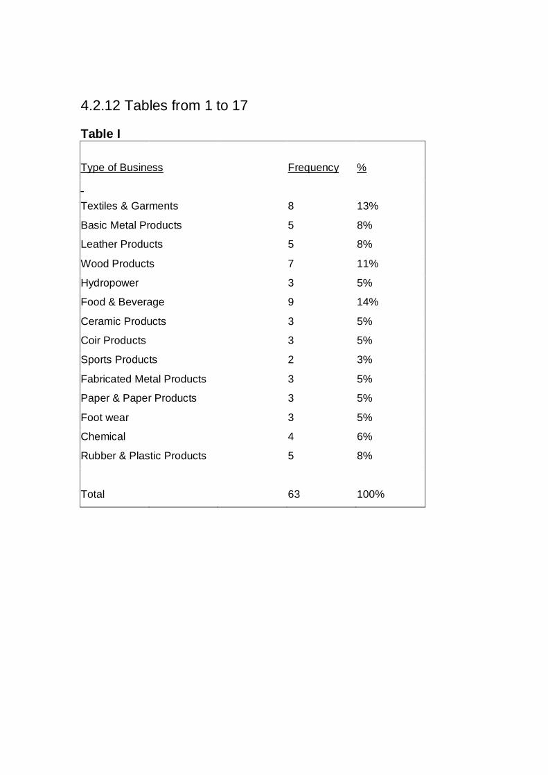
4.2.12 Tables from 1 to 17
Table I
Type of Business Frequency %
Textiles & Garments 8 13%
Basic Metal Products 5 8%
Leather Products 5 8%
Wood Products 7 11%
Hydropower 3 5%
Food & Beverage 9 14%
Ceramic Products 3 5%
Coir Products 3 5%
Sports Products 2 3%
Fabricated Metal Products 3 5%
Paper & Paper Products 3 5%
Foot wear 3 5%
Chemical 4 6%
Rubber & Plastic Products 5 8%
Total 63 100%

Table 2 Share Capital in million Rs Frequency %
50 – 100 11 17%
101 – 200 8 13%
201 – 300 9 14%
301 – 400 8 13%
401 – 500 8 13%
501 – 600 4 6%
601 – 700 4 6%
701 – 800 3 5%
801 – 900 4 6%
901 - 1000 4 6%
Total 63 100%

Table 3
Average Frequency %
Turnover in million Rs
1000 - 2000 9 14%
2001 - 3000 10 16%
3001 - 4000 10 16%
4001 - 5000 8 13%
5001 - 6000 8 13%
6001 - 7000 5 8%
7001 - 8000 5 8%
8001 - 9000 4 6%
9001 - 10000 4 6%
Total 63 100%

Table 4
Staff Frequency %
1000 - 2000 10 16%
2001 - 3000 14 22%
3001 - 4000 13 21%
4001 - 5000 14 22%
5001 - 6000 12 19%
Total 63 100%
Table 5
1st Priority 2nd Priority 3rd Priority
Valuation technique Frequency % Frequency % Frequency %
DCF 52 82.5% 6 10% 5 8%
Asset based 5 8,0% 26 41% 32 51%
Revaluation 6 9.5% 31 49% 26 41%
Total 63 100% 63 100% 63 100%

Table 6 SWOT Frequency %
Yes 59 82%
No 13 18%
Total 72 100%
Table 7
Forecast of Sales Revenue
Methods Frequency %
Time series 21 33%
Causal 39 62%
Delphi 3 5%
Total 63 100%

Table 8 Terminal value
Models Frequency %
Stable growth 37 59%
Multiple approach 4 6%
Liquidation value 22 35%
Total 63 100%
Table 9
Cost of Debt Frequency %
Borrowing rate of today 32 51%
Corrected rate for tax 31 49%
Total
63 100%
Table 10
Risk free rate Frequency %
Treasury bill 41 65%
Treasury bond 22 35%
Total 63 100%
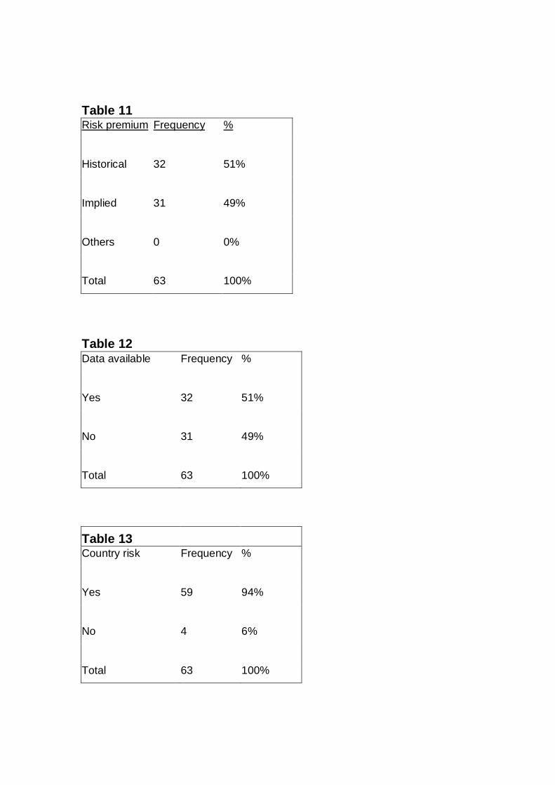
Table 11
Risk premium Frequency %
Historical 32 51%
Implied 31 49%
Others 0 0%
Total 63 100%
Table 12
Data available Frequency %
Yes 32 51%
No 31 49%
Total 63 100%
Table 13
Country risk Frequency %
Yes 59 94%
No 4 6%
Total 63 100%

Table 14
Beta estimate Frequency %
Regression 35 56%
Standard dev 25 40%
Earnings/Rev 2 3%
Others 1 2%
Total 63 100%
Table 15
Cost of equity Frequency %
CAPM 49 78%
APM 11 17%
Multifactor 3 5%
Others 0 0%
Total 63 100%

Table 16
Discount rate Frequency %
Cost of Capital WACC 53 84%
Others 10 16%
Total 63 100%
Table 17
DCF accuracy Frequency %
%
40 – 50 8 13%
51 – 60 3 5%
61 – 70 10 16%
71 – 80 20 32%
81 – 90 22 35%
91 – 100 0 0%
Total 63 100%
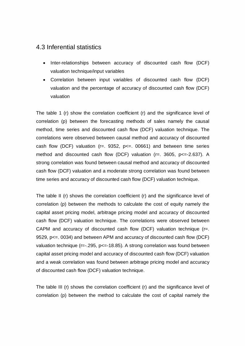
4.3 Inferential statistics
Inter-relationships between accuracy of discounted cash flow (DCF)
valuation technique/input variables
Correlation between input variables of discounted cash flow (DCF)
valuation and the percentage of accuracy of discounted cash flow (DCF)
valuation
The table 1 (r) show the correlation coefficient (r) and the significance level of
correlation (p) between the forecasting methods of sales namely the causal
method, time series and discounted cash flow (DCF) valuation technique. The
correlations were observed between causal method and accuracy of discounted
cash flow (DCF) valuation (r=. 9352, p<=. 00661) and between time series
method and discounted cash flow (DCF) valuation (r=. 3605, p<=-2.637). A
strong correlation was found between causal method and accuracy of discounted
cash flow (DCF) valuation and a moderate strong correlation was found between
time series and accuracy of discounted cash flow (DCF) valuation technique.
The table II (r) shows the correlation coefficient (r) and the significance level of
correlation (p) between the methods to calculate the cost of equity namely the
capital asset pricing model, arbitrage pricing model and accuracy of discounted
cash flow (DCF) valuation technique. The correlations were observed between
CAPM and accuracy of discounted cash flow (DCF) valuation technique (r=.
9529, p<=. 0034) and between APM and accuracy of discounted cash flow (DCF)
valuation technique (r=-.295, p<=-18.85). A strong correlation was found between
capital asset pricing model and accuracy of discounted cash flow (DCF) valuation
and a weak correlation was found between arbitrage pricing model and accuracy
of discounted cash flow (DCF) valuation technique.
The table III (r) shows the correlation coefficient (r) and the significance level of
correlation (p) between the method to calculate the cost of capital namely the

weighted average cost of capital (WACC) and accuracy of discounted cash flow
(DCF) valuation technique. The correlation was observed between WACC and
accuracy of discounted cash flow (DCF) valuation technique (r=. 9647, p<=.
00189). A strong correlation was found between weighted average cost of capital
(WACC) and accuracy of discounted cash flow (DCF) valuation technique.
The table IV (r) shows the correlation coefficient (r) and the significance level of
correlation (p) between the methods to calculate the risk factor () namely the
regression model, standard deviation model and accuracy of discounted cash
flow (DCF) valuation technique. The correlations were observed between
regression model and accuracy of discounted cash flow (DCF) valuation
technique (r=. 9352, p<=. 006615) and between standard deviation model and
accuracy of discounted cash flow (DCF) valuation technique (r=. 6576, p<=1). A
stronger correlation was found between regression model and accuracy of
discounted cash flow (DCF) valuation compared to the correlation between
standard deviation model and accuracy of discounted cash flow (DCF) valuation
technique.
The table V (r) shows the correlation coefficient (r) and the significance level of
correlation (p) between the methods to calculate the terminal value of the
business namely the stable growth model, liquidation value model and accuracy
of discounted cash flow (DCF) valuation technique. The correlations were
observed between stable growth model and accuracy of discounted cash flow
(DCF) valuation technique (r=. 9357, p<=. 006507) and between liquidation value
model and accuracy of discounted cash flow (DCF) valuation technique (r=.
5663, p<=1). A stronger correlation was found between stable growth model and
accuracy of discounted cash flow (DCF) valuation compared to the correlation
between liquidation value model and accuracy of discounted cash flow (DCF)
valuation technique.

4.3.1 Tables 1 (r) to v (r) Table I (r)
Accuracy of Frequency
Causal
method Time series
DCF %
40 – 50 8 0 7
51 – 60 3 1 2
61 – 70 10 3 5
71 – 80 20 18 2
81 – 90 22 17 5
91 – 100 0 0 0
Total 63 39 21
r 0.9352 0.3605
p <= 0.006614 <= -2.637
DF 4 4
Table II (r)
Accuracy of Frequency CAPM APM
DCF %
40 – 50 8 0 6
51 – 60 3 1 2
61 – 70 10 6 3
71 – 80 20 20 0
81 – 90 22 22 0
91 – 100 0 0 0
Total 63 49 11
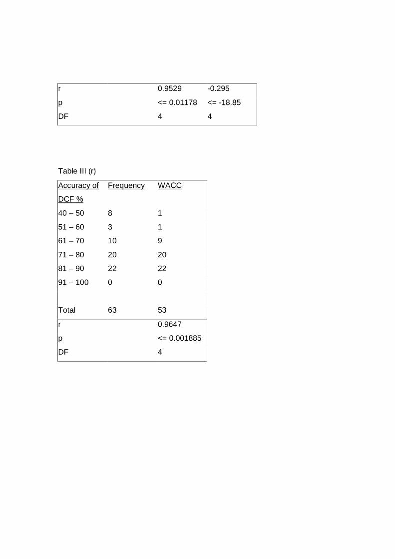
r 0.9529 -0.295
p <= 0.01178 <= -18.85
DF 4 4
Table III (r)
Accuracy of Frequency WACC
DCF %
40 – 50 8 1
51 – 60 3 1
61 – 70 10 9
71 – 80 20 20
81 – 90 22 22
91 – 100 0 0
Total 63 53
r 0.9647
p <= 0.001885
DF 4

Table IV (r)
Accuracy of Frequency Regression Peers
DCF %
40 – 50 8 0 5
51 – 60 3 1 2
61 – 70 10 3 7
71 – 80 20 13 7
81 – 90 22 18 4
91 – 100 0 0 0
Total 63 35 25
r 0.9352 0.6576
p <= 0.006615 <= 1
DF 4 4
Table V (r)
Accuracy of Frequency Stable growth
Liquidation
value
DCF %
40 – 50 8 1 5
51 – 60 3 1 2
61 – 70 10 2 6
71 – 80 20 14 6
81 – 90 22 19 3
91 – 100 0 0 0
Total 63 37 22

r 0.9357 0.5663
p <= 0.006507 <=1
DF 4 4
In addition to the above research study, researcher got the opportunity to
interview three more start up businesses with negative earnings. The participants
were of the view that discounted cash flow (DCF) valuation will not work for
number of reasons, too much uncertainty about the future and too much of the
value comes from the terminal value. They suggested that the new paradigms for
valuing their businesses often deviate significantly from what are viewed as first
principles in traditional valuation models.
Three fundamentals that determine the value of a business are its capacity to
generate cash flows from existing investments, the expected growth in these
cash flows over time and the uncertainty associated with whether these cash
flows will be generated in the first place. These fundamentals remain the same
no matter what type of business we are valuing large or small, manufacturing or
service and technology or non-technology, though the emphasis placed on each
may be different for different businesses.
In discounted cash flow (DCF) valuations, the relationship between fundamental
variables and value was made explicit by making assumptions about each, with
uncertainty showing up in the discount rate. In relative valuations, the relationship
is implicit and often shows up in the form of adjustments made to multiples when
businesses are compared to each other.
The participants were of the view that the cash flows from existing investments
are negative for their businesses, but their businesses usually have to generate
much higher positive cash flows in the future to compensate for their negative
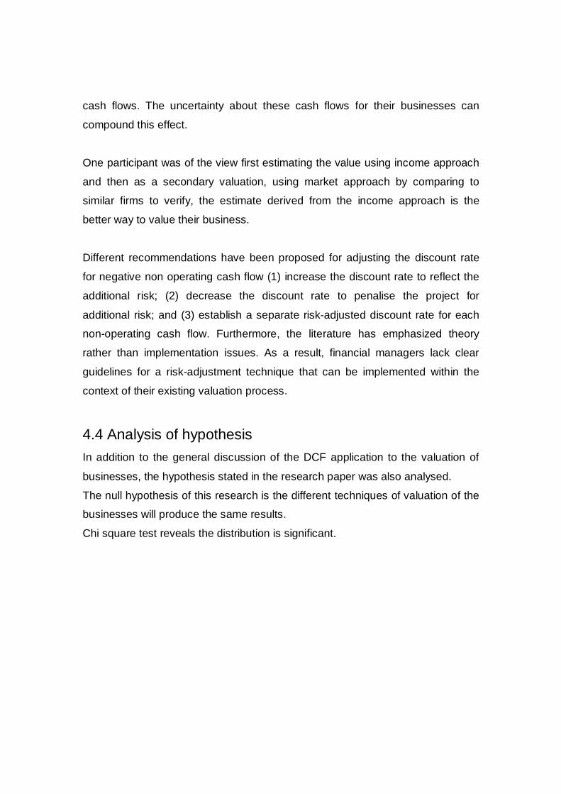
cash flows. The uncertainty about these cash flows for their businesses can
compound this effect.
One participant was of the view first estimating the value using income approach
and then as a secondary valuation, using market approach by comparing to
similar firms to verify, the estimate derived from the income approach is the
better way to value their business.
Different recommendations have been proposed for adjusting the discount rate
for negative non operating cash flow (1) increase the discount rate to reflect the
additional risk; (2) decrease the discount rate to penalise the project for
additional risk; and (3) establish a separate risk-adjusted discount rate for each
non-operating cash flow. Furthermore, the literature has emphasized theory
rather than implementation issues. As a result, financial managers lack clear
guidelines for a risk-adjustment technique that can be implemented within the
context of their existing valuation process.
4.4 Analysis of hypothesis In addition to the general discussion of the DCF application to the valuation of
businesses, the hypothesis stated in the research paper was also analysed.
The null hypothesis of this research is the different techniques of valuation of the
businesses will produce the same results.
Chi square test reveals the distribution is significant.
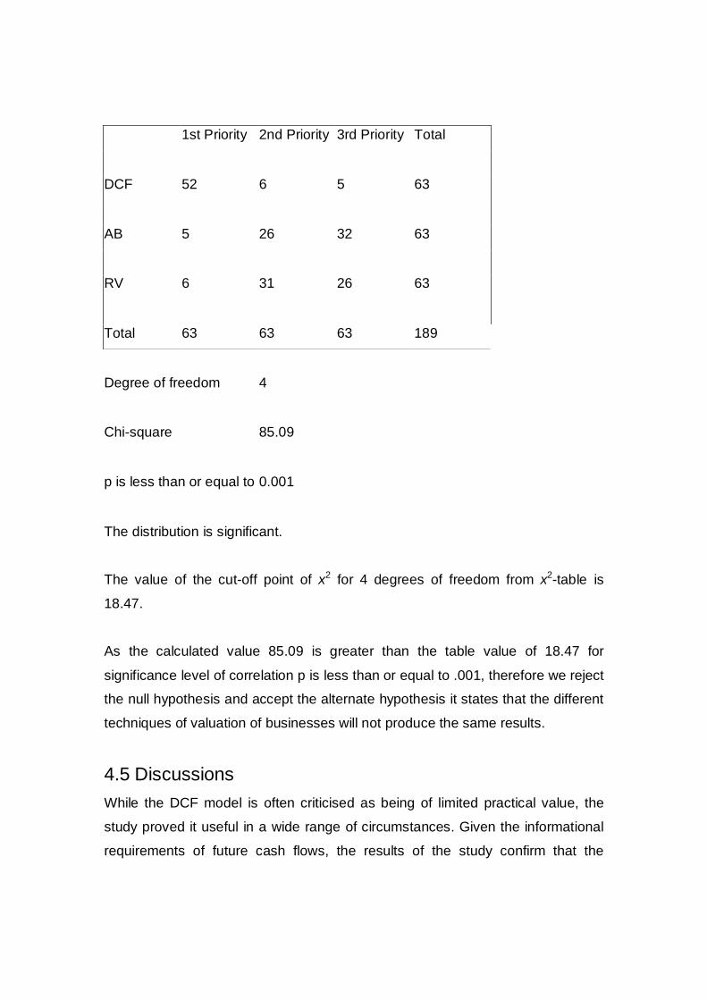
1st Priority 2nd Priority 3rd Priority Total
DCF 52 6 5 63
AB 5 26 32 63
RV 6 31 26 63
Total 63 63 63 189
Degree of freedom 4
Chi-square 85.09
p is less than or equal to 0.001
The distribution is significant.
The value of the cut-off point of x2 for 4 degrees of freedom from x2-table is
18.47.
As the calculated value 85.09 is greater than the table value of 18.47 for
significance level of correlation p is less than or equal to .001, therefore we reject
the null hypothesis and accept the alternate hypothesis it states that the different
techniques of valuation of businesses will not produce the same results.
4.5 Discussions While the DCF model is often criticised as being of limited practical value, the
study proved it useful in a wide range of circumstances. Given the informational
requirements of future cash flows, the results of the study confirm that the
approach is best used for businesses whose cash flows are currently positive
and can be estimated with some reliability for future periods.
An important additional consideration, which is that both the discounted cash flow
method and the dividend method are used to forecast the future cash flows, while
the intrinsic value method uses historical information. Taking the book value of
equity as an example, this has little to do with the market value of the equity and
the ratio of market value to book value is rarely equal to one. In fact, many
companies that have negative intrinsic value if one are using the book value of
equity as a measure. Book value is therefore not highly correlated with the
market value of the company or the market value of the equity.
Most of the participants were of the opinion that the best measure for
performance is to look at the discounted cash flow model of a company. The
comparison of the economic profits relative to the expectations of economic profit
is a one period measure, while the discounted cash flows attempt to look at the
performance of the company over many times into the future. According to some
of the respondents, correlations of the discounted cash flow estimates of the
value of a company with the actual market value of that company generally 82%
and above.
The accuracy and effectiveness of the different valuation techniques practices of
the businesses was considered by asking the participants of the organisations to
provide their evaluation of the degree of accuracy of their companies’ valuation
technique practices. More specifically, they were asked to identify the
uncertainties involved in calculating the inputs for business valuation techniques.
At the same time, they were also asked to state the limitations of the valuation
techniques used by them. Questions were also posed to the participants about
possible areas for improvement based on hindsight and lessons learned during
the past years.

According to 82.5% of participants, discounted cash flow analysis is the most
accurate and flexible method for valuing projects, divisions and companies. Any
analysis however is only as accurate as the forecasts it relates on. Errors in
estimating the key ingredients of business value can lead to mistakes in
valuation.
They were of the view that the discounted cash flow valuation method is an entity
or an enterprise approach where the cash flows from all sources of capital are
valued and then one subtracts the value of debt to get the value of equity. The
dividend discount model is an approach that is very similar in spirit. What it does
is it takes the free cash flows to the shareholders, discounts them at the cost of
equity and in fact one gets the same answer as with the enterprise approach.
During the research, some of the respondents said that the two items namely
operating lease and R&D expenses contradict the definition of operating income.
In order to correct the operating income, take the present value of operating
lease commitments, using the pre-tax cost of debt of the firm as the discount
rate, and treat the present value as debt. The operating income has to be
adjusted by adding back the operating lease expense and subtracting out the
depreciation created by the operating leases.
Specify the number of years before R&D can be expressed to generate
commercial products, collect R&D expenses from the past for that many years
and then amortize them. The remaining un-amortized R&D from prior years can
be considered the book value of the R&D asset, and operating income has to be
adjusted by adding back the R&D expense from the current year and subtracting
out the R&D amortization for the current year.
The actual taxes paid will reflect the fact that businesses save on taxes when
businesses make interest payments. The problem, however, is that business has
already counted the tax benefits in your cost of capital by using the after tax cost

of debt and increasing business cash flow for the same reason would be double
counting. This will result in a choice between effective and marginal tax rates.
The effective tax rate is lower than the marginal tax rate because companies
defer paying taxes. Since this is a tax saving, there is nothing wrong with using
the effective tax rate in computing the after tax operating income for last year and
even for the next few years. The best compromise is to use effective rates for the
early forecast years and move towards a marginal tax rate in the last years.
An analyst should expect the cost of capital to change for most businesses and
especially so for young businesses or businesses in transition. Not only can the
weights on debt and equity change, the other components such as cost of equity,
cost of debt and tax rate will change.
Generally, businesses that are young and risky have high costs of equity and
debt, little or no debt and high costs of capital. As the analyst expects these
businesses to grow and mature over time, he would expect the costs of equity
and debt to come down, the debt ratio to increase and the cost of capital to
decline.
The practical question is that an analyst will face is in coming up with these target
debt ratios and cost of funding. One is to look at industry averages, especially the
averages to mature businesses in the business for all of these components. The
other is to compute the optimal debt ratio with all the components for your
business.
In conventional practice, businesses are often valued with a constant debt ratio
and cost of capital over time. This is why there is much debate about whether
one should use actual debt ratio weights or target weights, with many analysts
arguing for the latter. Either extreme will be incorrect, with the former leading to
too low a value for young and risky businesses and the latter to too high a value.
The best compromise is to start with the actual debt ratio and move to the target
debt ratio over time.
Since it is not growth, that creates value but excess returns, the question can
really be framed as ‘How long will excess returns continue?’
One of the easiest ways to increase the value of a business is to push up the
stable growth rate towards the cost of capital. At first sight, therefore, it looks like
increasing the stable growth rate will always increase terminal value. However,
this is only true if the analyst is inconsistent in his assumptions. If the analyst
estimates the reinvestment rate as a function of the expected growth and return
on capital, then he sets up a trade off.
Reinvestment rate = Stable growth rate / Return on capital.
The trade off is as follows. If the analyst increases the stable growth rate, the
reinvestment rate will go up. Thus, while the analyst gains from growth, he will
lose in cash flows.
Terminal value = EBIT (1-t) (1- reinvestment rate)/ (cost of capital – g)
If the analyst assumes that the return on capital is equal to the cost of capital, the
gain from increasing growth will exactly be offset by the loss from having a higher
reinvestment rate, nullifying the effect of growth. In that case, the terminal value
will always be
Terminal value = EBIT (1-t) / cost of capital
If the analyst assumes that the business will earn more than its cost of capital in
perpetuity, increasing growth will increase value. If he assumes that it will earn

less than its cost of capital in perpetuity, increasing growth will reduce terminal
value.
The financial and operating environment is riskier today than what it was in the
past. This is evident from the following:
The last few decades have seen a substantial increase in the average
rate, as well as the volatility of inflation.
The increased uncertainty about inflation has been followed by greater
volatility in interest rates, exchange rates and commodity prices.
Global competition has intensified in the wake of reduced tariff barriers.
4.5.1 Risk and uncertainty In today’s world, managing corporate risks is a daunting task. In coping with the
challenge the following interrelated guidelines need to be considered.
Understand the firm’s strategic exposure.
Employ a mix of real and financial tools.
Proactively manage uncertainty
Align risk management with corporate strategy
Learn when it is worth reducing the risk.
Unlike in the past, the financial manager today has a bewildering number of ways
to hedge risk. If a business does not wish to bear certain types of risk, it can shift
the undesirable risk to others. This risk may have to do with interest rates, with
exchange rates, with stock prices or with commodity prices.

Derivatives can insulate cooperation from different types of risk. For example,
airlines may wish to hedge against rising fuel prices and can do this by buying an
option that rises in value with oil prices or a business may buy Japanese yen
forward to protect itself against adverse currency movements affecting its many
Japanese outlets.
What risk should be hedged and how much? There is no universal rule.
However, there are certain principles of hedging that warrant exploration before
we consider specific risk shifting devices. Before risk can be hedged, it first must
be identified. Exactly what kind of risk exposure is involved? Once identified,
businesses then try to quantify it with probabilities and perhaps with simulations.
The idea is to determine what is likely to happen if the underlying situation
changes. For example, if the source of the risk were interest rates, businesses
would like to know what happens to the value of their security or financing
position with a change in interest rates, knowing this, the idea in hedging is to
take a position opposite to the exposure. This can be with futures contracts, with
forward contracts, with options or with swaps.
These allow businesses to lock in a rate immediately but without having to pay
for them until a future date. They are calculated by using the current exchange
rate for the currency pair, the interest rates for the two currencies along with the
length of the contract. They value the current exchange rate for the future date
rather than trying to estimate where the market is heading.
Forward contracts will usually involve a deposit, which allows you the luxury of
being able to utilise the majority of your capital until the end of the forward
contract. They also reduce your market risk by locking in a rate now even though
the actual transaction is not taking place until a later date. This allows the
business to cost your purchases today and in doing so, effectively lock in your
profits.

Businesses would like to affect a perfect hedge, but this usually is not possible.
The value of our position and the value of the instrument used to hedge do not
move completely in concert. Usually there are slight to moderate deviations.
Hedging is important, especially in a market with flexible exchange rates, as it
permits exporters and importers to protect themselves against risks concerned
with exchange rate fluctuations, thus enabling them to concentrate on their pure
trading functions. It should, however, be observed that the forward market is a
short run market, in which the contract period is usually three months.
As per Adrian J. Slywotzky and John Drzik, businesses insured and hedged
against many risks – but not for the greatest ones, the strategic risks that can
disrupt or even destroy your business. Learn to anticipate and manage these
threats systematically and, in the process, turn some of them into growth
opportunities.
The discipline of risk management has made considerable progress in recent
years. Corporate treasurers and chief financial officers have become adept at
quantifying and managing a wide range of risks: financial for example currency
fluctuations, hazard (chemical spills), and operational (computer system failures).
They defend themselves against these risks through now tried-and true tools
such as hedging, insurance, and backup systems.
Most managers have not yet systematically addressed the strategic risks that can
be a much more serious cause of value destruction. Strategic risks take a variety
of forms that go beyond such familiar challenges as the possible failure of an
acquisition or a product launch. A new technology may overtake your product.
Gradual shifts in the market may slowly erode one of your brands beyond the
point of viability. Alternatively, rapidly shifting customer priorities may suddenly
change your industry.

The key to surviving strategic risks knows how to assess and respond to them.
Devoting the resources to do this is well worth it. Many businesses already
commit themselves to meticulously managing even relatively small risks-for
instance, auditing their invoices to comply with new corporate governance
regulations. These businesses can realize even greater value by taking a
disciplined and systematic approach to mitigating the strategic risks that can
make or break them.
Of course, no business can anticipate all risk events: there will always be
unpreventable surprises that can damage the business. When a risk is common
to all businesses in an industry, taking early steps to mitigate it can put your
business in a much stronger competitive position. Moreover, many strategic risks
mask growth opportunities.
By managing strategic risk, you can position your company as a risk shaper that
is both more aggressive and more prudent in pursuing new growth. Such benefits
make strategic risk management a crucial capability both for chief financial
officers, who need to protect the stability of their businesses and for any senior
managers looking for sources of sustainable growth.
Adrian J Slywotzky and John Drzik categorized strategic risk into seven major
classes: industry, technology, brand, competitor, customer, project, and
stagnation.
They are on the view that a new relationship between risk and reward is thus
emerging. While managers often see a trade-off between the two, creative risk
management combined with a good business model can allow a company to
improve in both areas. This shift is analogous to the evolution of thinking about
the relationship between cost and quality.

Thirty years ago, managers believed there was a trade-off in which higher quality
meant higher cost. Pioneering Japanese manufacturers turned that thinking
around by showing that improving the system could actually reduce costs while
simultaneously raising standards of quality.
Similarly, the challenge for managers today is to help their businesses move to a
position of lower risks but higher financial returns. With the right mind-set and
timely deployment of countermeasures, businesses can manage the full
spectrum of risks they face and find that risk/reward sweet spot.
Thomas Jefferson once observed, “Constant vigilance is the price of freedom”.
We live in an era of outlandish expectations, animated by a pervasive cultural
craving for personal wealth and instant gratification. Businesspeople and
investors must be ever vigilant if they are to remain free from conflict,
complications, losses, and lawsuits.
Risk can have different meanings but a common understanding is that the event
associated with the risk could actually happen, and the consequences of this risk
might not be pleasant.
The effective management of risk is central to providing a safe and healthy
workplace. Risk management should be an essential part of the continuous and
structured planning cycle within a business.
One of the key objectives of the investment appraisal system is to allow sensible
allocation of the scarce resource-money. It is necessary that new investments fit
within the long-term corporate strategy. (STEEP) sociological, technological,
ecological, economic and political factors must be taken into account in the
feasibility study of the project especially in the case of developing countries like
Sri Lanka.

Market perception, customer reaction, competitor reaction, producer reaction,
supplier reaction, and employee reaction, even government reaction all need to
be taken into account when considering forecast of free cash flows. One of the
key roles of an investment appraisal committee is to consider whether borrowing
for a particular project should be segregated from the normal borrowings.
Including the project within a broad portfolio, employing sophisticated financing
techniques such as forward rate agreement and options or setting up secured
financing with fixed rates of return, can insulate rate of return changes of a
project.
Once a project is underway, the organisation needs to begin a process of post-
audits where expected cash flows and costs are compared with the actual costs
and cash flows. Any differences that arise may be grouped into two areas: those
resulting from factors outside the control of the organisation and those within the
control of the organisation, from these results the organisation may respond by
altering its future investment appraisal techniques. It has generally been
observed that the best-run organisations are those, which place the greatest
emphasis on the post audit approach.
4.5.2 Valuation of businesses under distress In most valuations, we ignore distress entirely and make implicit assumptions
that are often unrealistic about the consequences of a firm being unable to meet
its financial obligations. Even those valuations that claim to consider the effect of
distress do so incompletely. The CFOs of the businesses should use their core-
competences to find ways how to incorporate the effects of distress into business
valuation techniques.
In both discounted cash flow and relative valuation, we implicitly assume that the
businesses that we are valuing are going concerns and that any financial distress
expected is temporary. Behind this, a significant amount of value comes from

terminal value, the present value of which add to the present value of future free
cash flows of the business in calculating the value of the business. However, if
the distress is not temporary and there is a real chance that the business will not
survive to get to the terminal value.
Growth is inevitable and businesses may not remain as going concerns. In fact,
even large businesses can become financial distress for one reason or the other
and the consequences for value can be serious. In fact, even casual empirical
observation suggests that a very large number of firms, especially smaller and
higher growth, will not survive and will go out of business. Some will fail because
they borrow money to fund their operations and then are unable to make these
debt payments. Other may fail because they do not have the cash to cover their
operating needs.
The consequences of financial failure is that businesses that are unable to make
their debt payments or the operating payments have to liquidate their assets and
use the proceeds to pay off the debt or operating payments and any left over will
be paid out to equity investors. These liquidation costs can be considered the
direct costs of bankruptcy.
In fact, the costs of distress stretch far beyond the conventional costs of
bankruptcy and liquidation. The perception of distress can do serious damage to
a business’s operations as employees, suppliers, customers and lenders react.
Businesses that are viewed as distressed lose customers that result in loss of
sales to the business.
There will be high employee turnover and tighter restrictions from suppliers than
healthy businesses. These indirect costs of bankruptcy can be a burden for many
businesses. According to some of the participants, this cost may be in the region
of 10 to 25% of the business value. Therefore, the cost of distress is a significant

amount cannot be ignored in valuation. The question now is how best we can
adjust business value for the potential for distress.
Considering the calculation of value of a business under discounted cash flow
method, the assumption in this approach is that a business is a going concern,
with potentially an infinite life. The terminal value is usually estimated by if
earnings grow at a constant rate (a perpetual growth rate) forever. Given the
likelihood and consequences of distress, it seems imprudent to assume that we
can ignore this possibility when valuing a business, and particularly the
businesses, which are in poor health and with substantial debt obligations.
The arguments offered by proponents of discounted cash flow valuation for not
considering the possibility of businesses failing are as follows:
We value only large, publicly traded businesses and distress is very
unlikely for these businesses.
We assume that access to capital is unconstrained.
We adjust the discount rate for the possibility of distress.
We adjust the expected cash flows for the possibility of distress.
We assume that even in distress, the firm will be able to receive the
present value of expected cash flows from its assets as proceeds from the
sale.
4.5.3 Adapting discounted cash flow valuation to distress situations If the likelihood of distress is high, access to capital is constrained by internal or
external factors, then the distress sale proceeds will be lower than the going
concern values, discounted cash flow valuations will overstate business and
equity value for distressed businesses, even if the cash flows and the discount
rates are correctly estimated.
We estimate expected values for each of the input variables in traditional
valuation. For example, in valuing a firm, we may assume an expected growth

rate in revenues of 25% a year and the expected operating margins will be 10%.
In reality, these variables have a distribution of values, which we condense into
an expected value. If we look at the entire distribution, we will be able to
incorporate distress in valuation by using simulations.
To use simulations, first, we will have to decide the circumstances under which,
distress will constitute and what will happen in the event of distress. For example,
the cumulative operating losses of more than LKR 500 million over three years
will push the business into distress and in this case, it would sell its assets for
25% of book value. A business that has three bad years in a row in a healthy
economy with rising equity markets may be having less chance to default than a
similar business in the middle of recession.
The limitation of simulation analysis is the information that is required to work for
it. In practice, it is difficult to choose both the right distribution to describe a
variable and the parameters of that distribution. When these choices are made
carelessly or randomly, the output from the simulations conveys no valuable
information.
To consider the effects of distress into a discounted cash flow valuation, we have
to incorporate the probability that a business will not survive into the expected
cash flows. We have to consider all possible scenarios ranging from the most
optimistic to the most pessimistic. Then we have to assign probabilities to each
scenario and multiply the cash flows by these probabilities in order to estimate
the expected cash flows each year.
J=n
Expected cash flow = jt (Cashflowjt)
J=1
Where: jt is the probability of scenario j in period t and

cashflowjt is the cash flow under that scenario and in that period.
These estimates have to be estimated each year, since the probabilities and the
cash flows are likely to change from year to year. Alternatively, we can estimate
the going concern scenario and the distress scenario.
Expected cash flow t = (Cash flowgoing concern)* going concern + (Cash flowdistress)*(1-
going concern)
Where going concern is the cumulative probability that the firm will continue as a
going concern through period t.
Estimating Discount Rate The risk free rate is the starting point for all expected return models. For an asset
to be risk free, it has to satisfy two conditions. There can be no risk of default
associated with its cash flows and there can be no reinvestment risk. In practice,
however, it is usually appropriate to match up the duration of the risk free asset
to the duration of the cash flows being analysed. In corporate finance and
valuation, this will lead us towards long-term government bond rates as risk free
rates.
It is also important that the risk free rate be consistent with the cash flows being
discounted. In particular, the currency in which the risk free rate is denominated
and whether it is a real or nominated risk free rate should be determined by the
currency in which the cash flows are estimated and whether the estimation is
done in real or nominated terms.
In valuing a business, we often use regression beta in estimating cost of equity
and the cost of debt by looking at the prevailing interest rate of treasury bonds.
These approaches can lead to inconsistent estimates for businesses with a
significant probability of distress. Since regression, betas are based on past

prices over a period of two to five years, but distress occurs over short periods,
therefore we will find that these betas will understate the real risk in the
distressed business.
To estimate the cost of equity we have to calculate more reasonable estimate
than regression betas. Instead of using regression betas, we could use the
bottom-up levered beta and the current market debt to equity ratio of the
business. Since distressed businesses have high debt to equity ratios, this will
lead to levered betas that are significantly higher than regression betas. In
reality, most distressed businesses are not in a position to get any tax advantage
from debt; the levered beta will become even higher.
Levered beta = Bottom-up un-levered beta (1+ (1- tax rate) (debt / equity))
It is reasonable to re-estimate debt to equity ratios and tax rates for future years
based upon the expectations for the business and adjust the beta to reflect these
changes.
In addition to the market risk, we could add a distress factor to cost of equity.
This would result in cost of equity of distressed businesses much higher than
healthy businesses in the same business.
To estimate the cost of debt for a distressed firm, it would be better to use the
interest rate based upon the firm’s bond rating. To compute the cost of capital,
we need to estimate the weights on debt on equity. In the initial year, we should
use the current market debt to capital ratios. As we make our forecasts for future
years and build in our expectations of improvements in profitability, should adjust
the debt ratio towards more reasonable levels.

The biggest limitation in using this approach is that it is difficult to estimate the
cumulative probabilities of distress and survival each year for the forecast period.
As a result, the expected cash flows may not incorporate the effects of distress
completely. The other limitation is it is difficult to bring both the going concern
and the distressed firm assumptions into the same model.
Dealing with distress separately
To value the effects of distress, estimate the cumulative probability that the firm
will become distressed over the forecast period, and the proceeds will get form
the distress sale. The value of the firm can then be written as:
Firm Value = Going concern value * (1 - Distress)+ Distress sale value* Distress
Where distress is the cumulative probability of distress over the valuation period
this makes valuation simpler and it allows making consistent assumptions within
each valuation.
If we consider the distress sale value to be a version of liquidation value, and if
we assume that the probability of distress is one, the firm value will in fact
converge on liquidation value. The advantage of this approach is that it allows us
to consider the possibility that even distressed firms have a chance of becoming
going concerns.
Going concern DCF To value a firm as a going concern, the expected cash flow is estimated only
across the scenarios where the firm can survive and thus should be higher than
the expected cash flow was estimated in the modified discounted cash flow
model. When discounting discount rates, the assumption is that debt ratios will in
fact decrease over time, if the firm is over levered, and that the firm will derive tax
benefits from debt as it turns the corner on profitability. This is consistent with the
assumption that the firm will remain a going concern. Most discounted cash flow
valuations that we observe in practice are going concern valuations.

A better way to deal with the risk of truncation would be to do the following. First,
assume that your firm will be a going concern and do a discounted cash flow
valuation of it. Second, assess the probability that your firm will not be a going
concern: a good place to look would be the bond market if the company has
bonds outstanding. Third, estimate the distress value of the assets in the event of
bankruptcy. Finally, compute the expected value of the firm = probability of going
concern * DCF value + probability of distress * distress sale value
The analyst would need to subtract out the market value of anything that
considered debt for the cost of capital calculation. Thus, the analyst should
subtract out the market value of all interest bearing debt, short as well as long
term, and the present value of operating leases and other off-balance sheet debt
that you can identify. An alternative is doing a liquidation valuation of the assets
of the firm and subtract out the book value of the debt outstanding.
4.5.4 Valuing high growth businesses In general, it is easy to value businesses, which are stable and matured. For
these types of businesses, it is easy to predict the future cash flows. Therefore,
valuation models such as discounted cash flow (DCF) works reasonably well on
these types of businesses. In contrast, valuing high growth businesses is
complex.
These businesses have limited history to work on for future projections. Heavy
investments in the early periods will result in negative cash flows in these high
growth businesses. It is hard to use a discounted cash flow (DCF) valuation
approach or price to earning (P/E) ratio when a business has negative cash flow.
Many innovative valuation methods were emerged to overcome the situation of
negative cash flows in businesses.

It is increasingly apparent that the financial value of a firm depends on intangible
assets (e.g. brands, customers, employees, knowledge) that are not on the
balance sheet. According to Sunil Gupta, Donald R Lehmann and Jennifer Ames
Stuart’s approach uses the well-established finance approach of discounted cash
flow (DCF). However, by using it at a customer level they were able to provide a
useful method for forecasting the stream of future earnings, a key input to any
valuation model. They were demonstrated how valuing customers make it
feasible to value firms, including high growth firms with negative earnings.
They defined the value of a customer to a firm as the expected sum of
discounted future earnings based on key assumptions concerning retention rate
and profit margins. The value of all customers is determined by the acquisition
rate and cost of acquiring new customers.
They compared the relative impact of improving retention, margins and
acquisition costs. The results were shown that retention elasticity is in the range
of 3-7. In other words, improving customer retention by 1% is likely to improve
customer and firm value by 3-7%. In comparison, margin elasticity is about one
and acquisition elasticity is only .02 - .03. They were also found that 1%
improvement in discount rate or cost of capital. Their results were suggested that
the linking of marketing concepts to shareholder value is both possible and
insightful.
One popular measure to emerge in 1999 – 2000 was the number of customers.
This metric was based on the assumption that growth companies need to acquire
customers rapidly in order to gain first mover advantage and build strong network
externalities, at times regardless of the cost involved (The Wall Street Journal,
Nov 22, 1999).
Academic research by Trueman, Wong and Zhang (2000) combined financial
information with the non-financial information for 63 businesses for the period

September 1998 to December 1999. A regression of market value on these
components revealed that while bottom line net income had no relationship with
stock price, both unique visitors as well as page views added significant
explanatory power.
A related study by Demers and Lev (2001) used similar data for 84 businesses
for 1999-2000 to examine the relationship between market value and non-
financial measures. They found that non-financial measures such as reach i.e.
number of unique visitors and stickiness i.e. site’s ability to hold its customers
explain share prices of high growth businesses.
These studies are correlation in nature and assume that the market value
represents the true intrinsic value of the business at any time – an efficient
market argument. However, even if the markets are efficient in the end, recent
history suggests significant deviations exist in the short run. In other words,
dependent variable in these studies is likely to change significantly over time,
which may alter conclusions about the value of customers. Partly because of this,
financial analysts are now quite sceptical about non-financial metrics, especially
number of customers.
Companies in the high tech industry are continuously facing challenges to
innovate their products and services in order to sustain their competitiveness. To
be the market leader in this highly competitive industry, characterized by ever-
evolving technology benchmarks, requires speed and flexibility.
Herein Intangible assets like technological capability, intellectual property,
business processes, experience curve based learning efficiencies, network of
highly skilled partners, customer relationships provide the critical competitive
advantage and drive the profitability of the firm in the industry. However, these
are not reflected in the balance sheet of the companies.
Hi-tech firms, in initial stages, need to incur huge costs in building up these
critical assets, which are expected to generate cash flows in subsequent periods.
These costs are not capitalised but are expensed in the period in which are
incurred and this results in losses by a high tech firm in its initial stages.
A valuation model based on either cash flows or earnings will fail to value the firm
appropriately, unless cash flows are estimated over a sufficiently long period as
these investments reduce cash flows and earnings in the short term. Moreover,
even the estimation of cash flows itself is a challenge as high tech companies are
characterised by high growth, high uncertainty and high losses in the transient
phase.
High tech companies boosted by their competitive advantage are expected to
enjoy higher profit margins, characterised by speed and flexibility and driven by
market conditions are expected to experience higher grow rates, however their
returns are much more risky. Comparables like Price Earnings ratio or Revenue
Multiples are difficult to employ due to the uniqueness in prospects of each
individual company.
Further, in a high tech company, characterised by negative earnings and high
revenue growth, multiples cannot be used for valuation. Moreover, the multiples
estimated based on past data are not applicable in the fast changing
environment.
The cost approach in valuation of high tech companies attempts to measure the
replacement cost. This approach is based on the logic that the fair market value
can be no more than the cost of acquiring a substitute with same features and
functionalities. It values a company based on the estimation of costs incurred or
investment required to replace the future earning ability of the firm and its assets.

The cost approach is not appropriate to value high tech companies with valuable
intangible assets. It ignores the value of intangible assets and the opportunity
costs of earnings. The benefits of an intangible asset like creativity, innovation
may exceed costs incurred in its acquisition. The approach equates value to the
costs incurred and does not measure the value of future benefits likely to accrue
because of investments made.
The market approach measures the present value of future benefits based on
market estimate. It involves identifying actively traded comparable companies
within the industry and using their multiples to estimate the business’s fair market
value. It becomes difficult to use this approach for valuation of high tech
companies, as their uniqueness and asset specificity makes it difficult to find
comparable businesses and appropriate multiples. Moreover, the lack of active
markets in the specific assets owned by high tech companies make it difficult to
use this method in valuation.
Further, the multiples do not provide reasonable results in case of high tech
companies specially those in the initial stages when huge investments
significantly reduce the cash flows, earnings and net-income. Negative earnings
may give meaningless results.
Moreover, in rapidly changing environment, the multiples obtained based on
past data are not applicable in the changed environment. However, the market
approach can be used to crosscheck the valuation obtained by other
approaches. Industry ratios and multiples provide confidence in the assumptions
made to arrive at the valuation using other approaches.
Using the modified discounted cash flow (DCF) valuation approach, considering
other factors such as investment risk and valuation of intangible assets and
taking into consideration the option value of flexibility and uncertainty, we can
generate reasonable valuation estimates for the high tech companies. This

modified approach is by no means perfect and will not eliminate the uncertainty
in valuation of high tech companies but the impact of these critical issues can be
factored.
In recent years, firms have turned to their attention increasingly to ways in which
they can increase their value. A number of competing measures, each with
claims to being the best approach to value creation, have been developed and
marketed by investment banking firms and consulting firms.
Value enhancement is clearly on the minds of many managers today. As they
look at various approaches to value enhancement, they should consider a few
facts. The first is that no value enhancement mechanism will work at generating
value unless there is a commitment on the part of managers to making value
maximisation their primary objective. Value creation is hard work in competitive
markets and almost involves a trade off between costs and benefits.
Based on the above discussion, it is evident that the majority of the businesses in
this research study use discounted cash flow (DCF) valuation technique to value
their businesses.

Chapter 5 Recommendations and implications
5.1 Introduction Valuation is the process of estimating price. However, regardless of the
technique used, the valuation will be affected by uncertainties namely uncertainty
in the comparable data available, uncertainty in the current and future market
conditions and uncertainty in the specific inputs for the business. These input
uncertainties will translate into an uncertainty with the output figure, the estimate
of price.
The purpose of any valuation is to determine the present value of a future cash
flow. The value of an investment is the discounted value of all estimated future
liabilities and benefits. Value is therefore based on future forecasts, which can be
modelled either implicitly or explicitly. In cases where the cash flow is subject to
variation of growth, this best estimate becomes less certain. Thus, valuations are
uncertain.
The more accurate the future expectations the more robust the valuation of the
business will be. This highlights the importance of dealing with future
expectations in the valuation process and suggests that the adoption of multiple
scenarios will greatly facilitate the Analyst in providing sound competency in
valuing the business.
5.2 Summary The history of discounted cash flow evaluation goes back to the 1930’s and the
work by Modigliani and Miller in the late 1950 introduced a more modern
approach to the subject. They were followed by many other scholars, including
Malkieland then Alfred Rappaport who took the formula approach and turned it
into a spreadsheet approach, which is used by most people these days.
Copeland have done valuations of businesses in 30 to 40 different countries and
found that the discounted cash flow approach for business valuation works
equally well in Japan, Germany, US and in Brazil.
Kaplan and Ruback (1995) examine the discounted cash flow (DCF) approach in
the context of highly leveraged transactions such as management buyouts and
investments. They found that transaction prices are close to the present value of
projected cash flows, although they are unable to reject the hypothesis that the
projections are made to justify the price.
Kaplan and Ruback report that a capital asset pricing model (CAPM) based
discounted cash flow (DCF) valuation approach has approximately the same
valuation accuracy as a comparable firm’s valuation approach with earnings
before interest, taxes, depreciation, and amortization as the accounting measure
being capitalised. Their sample firms are typically large and mature firms.
Gilson, Hotchkiss, and Ruback (1998) also find that, for firms emerging from
bankruptcy, discounted cash flow (DCF) valuations have the same degree of
accuracy as valuations based upon comparable firm multiples. They show that
the economic interests of various parties in the bankruptcy proceedings affect the
cash flow forecasts that are used.
The scientific method could be applied to a discipline like valuation. Over the
centuries, people have tried different approaches to different methodologies for
valuing companies and the approach the discounted cash flow (DCF) has stood
the test of time better than any other approach. Articles on this subject have been
published in leading journals.
One that was published a few years ago by Kaplan and Ruback (journal of
Finance, 1996), which examined the discounted cash flows against valuation
multiples, found that discounted cash flows did better statistically. A surviving
methodology would seem to be the one that best explains the reality that we

observe and so far the survivor seems to be the discounted cash flow valuation
method, at least where large firms are concerned.
5.3 Recommendations In order for a mathematical model, as the discounted cash flow (DCF) model, to
have high quality in its results, the quality of the in-data is important. The in-data
discussed in the study was the future cash flow and especially the future sales
since they are the most influential factor to derive the future cash flows.
The future sales and the future cash flows were identified as uncertain.
Therefore, they have to be estimated. When estimating the future sales there are
two difficulties to overcome (1) a subjective element enters the valuation and (2)
the accuracy of the forecast highly affects the accuracy of the valuation.
To improve the discounted cash flow (DCF) model the implication of these
difficulties should be accounted for. To overcome the subjectivity of the
valuations analysts should strive to make their valuations as scientific as
possible. The argument is that this could be made by implementing quantitative
methods to achieve objective forecasts and by applying the scientific method in
how the analysis is conducted and above all how the results are reported. This
implies that there should be a structure in the analysis process resting on
scientific method.
The scientific part of using quantitative models should be focussed on
implementation and refining of simulation models. This is to quantify the risks of
inaccurate assumptions and estimations and to gain further knowledge about the
factors that affect the results and the interconnections among themselves.
If we acknowledge that we, by necessity, cannot have certain results, or final
truths, the second best is to create an approach that has unlimited capabilities of
improvement. This is achieved by applying the theory of the open society to the

discounted cash flow (DCF) method and the valuation process. This can be
achieved by making analysts abide to ethical argumentation that rests on
reasonable arguments. The best way of achieving all this might be through
causal model approach (CMA).
The reasons behind this conclusion are that the model lends itself easily to
simulation, and the structure of the model makes it easy to state explicitly
estimations and how is the valuation of businesses get affected by changes in
the environment. The research supports the conclusion of the causal model
approach (CMA). It establishes that the causal method approach (CMA) is a
possible approach but it has important limitations.
There are practical problems in applying causal method approach (CMA); still
participants believe that it is of interest to apply the approach. This since the
approach gives an understanding of how the environment affects the sales that
can be valuable when conducting other forecasts and because the approach is
easily applied to sensitivity analysis.
However, these limitations indicate that the application of another forecasting
model, such as a time series model, should be implemented as well. By applying
forecasting model with different weaknesses, more useful and important
conclusions concerning the probable future of a business can be formed.
Thus, the main conclusion is that, to improve the discounted cash flow (DCF)
method, analysts should strive to make the valuation process as scientific as
possible. Strive to make as reasonable and ethical arguments as possible and to
state explicitly their assumptions and subjective views.
Use a causal model approach (CMA) as a guide when translating the strategic
perspective to the financial forecast. It is prudent to use more than one
forecasting model is applied. Finally, causal method approach (CMA) for

forecasting future sales, about 80% of the respondents feel that it has contributed
to the continuous process of improvement of the discounted cash flow (DCF)
method.
Over the last three decades, the capital asset pricing model (CAPM) has
occupied a central and often controversial place in most corporate finance
analysts’ tool. The model requires three inputs a risk free rate, a beta and an
expected risk premium for the market portfolio to compute expected returns.
Models of risk and return in finance require us to estimate the exposure of a
business to market risk, relative to other businesses in the market. The
conventional estimate of this relative risk, measured by regressing stock returns
against a market index is flawed because the market index can be dominated by
a few stocks, the business itself might have changed during the course of the
regression.
While these regression betas can be modified to reflect financial fundamentals
and there exist measures of relative risk that do not require a regression, the
bottom up approach has the most promise when it comes to delivering updated
betas for most businesses. In the bottom-up approach the beta for a business is
estimated as the weighted average of the un-levered betas of the different
businesses that the business operates in, adjusted to reflect both the current
operating and financial advantage of the business.
According to researcher's opinion, much more effort should be put into the
development of a risk and return market model to determine the appropriate
discount rate. This is the critical ingredient in discounted cash flow valuation.
Errors in estimating the discount rate or mismatching cash flows and discount
rates can lead to serious errors in valuation. The discount rate used should be
consistent with both the risk and the type of cash flow being discounted. The
currency in which the cash flows are estimated should also be the currency in
which the discount rate is estimated.
If the business calculates the value of its equity by discounting cash flows to
equity, the discount rate to be used in this valuation is cost of equity. On the
other hand, if the business calculates the value of its firm by discounting cash
flows to firm, the discount rate to be used in this valuation is cost of capital.
If the business is large and growing at a rate close to or less than growth rate of
the economy, or constrained by regulation from growing faster than the economy
is a stable firm has average risk. For this type of businesses, stable growth
model can be used to calculate the terminal value of a business.
If the business is large and growing at a moderate rate i.e. less than or equal to
overall growth rate plus 10% or has a single product and barriers to entry with a
finite life, then it is advisable to use a 2-stage growth model. If the business is
small and growing at a very high rate i.e. greater than overall growth rate plus
10% or has significant barriers to entry into the business, then use a 3-stage or
n-stage model.
There is no commonly held definition of due diligence, nor is there any standard
legal definition. The following definition is useful in understanding the purpose of
due diligence.
Due diligence is the process of investigation and evaluation, performed by
investors, into the details of a potential investment, such as an examination of
operations and management and the verification of material facts. Most of us
think that due diligence is the first step before negotiating the purchase or sale of
a professional practice. In reality, this is not the case. The due diligence process
reveals significant confidential information, is very time consuming.
Prior to investing time in due diligence, the buyer and the seller should have at
least the framework of a deal crafted. The parties should exchange generic but
specific, detailed information about their respective businesses. If an agreement
can be reached based on this information, it is then appropriate to commence a
due diligence review.
Generally, due diligence refers to the care a reasonable person should take
before entering into an agreement or transaction with another party. Due
diligence is essentially a way of preventing unnecessary harm to either party, or
the entity involved, in a transaction.
The care that a prudent person might be expected to exercise in the examination
and evaluation of risks affecting a business transaction. Buying or selling a
business is a strenuous job, yet potentially rewarding process. Buying a business
involves investing a fair amount of money and time. It is very important to
conduct due diligence when gathering information about the business. In fact,
personnel net worth should never be under valued for personal worth.
Conducting proper due diligence will help the buyer to find out bad financial
situation, pending law suits, contingent liabilities, working condition of plant and
machineries, employees’ skills, marketing, contractual obligations, reputation,
regulatory compliance, ownership, competition and all other vital factors that may
affect the present value and future viability of the enterprise. There is no set
amount of time that must pass during due diligence, one can take as long as
need to answer all their questions.
Essentially a homework exercise, due diligence generally requires input from a
multidisciplinary team galvanized by the time-honoured admonition of caveat
emptor or buyer beware. In other words, investors have the obligation to look out
for themselves. Buyer should have questioned carefully about himself and his

business background, not tactlessly but in an inquisitive and non-threatening
manner, to probe for specifics about his career and prior business relationship.
Too often, the analysis preceding the acquisition of or investment in a new
business concentrates on financial matters and neglecting other critical factors
that can affect the decision, such as environmental exposures, suppliers
contracts, condition of plant and machineries, political stability, technical skill of
the employees, marketing and many other factors.
Identifying defects should be the primary objective. The aim is to obtain full
disclosure of the relative strengths and weaknesses of the business as well as
the opportunities and threats posing the business. To achieve this catalyst to be
used is due diligence.
In fact, entrepreneurs never expect to fail. For most of them, failure is not even a
possibility, let alone a probability. In truth, most businesses and start-ups and
acquisitions have major flaws, some even fatal and identifying them should be
the first priority when making any deal. Such scepticism is the corner stone when
it comes to managing the risk.
Because the financial forecasts are unreliable, senior management cannot
confidently tie capital approval to strategic planning. Consequently, strategy
development and resource allocation become decoupled, and the annual
operating plan ends up driving the company’s long-term investments and
strategy.
Without credible financial forecasts, top management cannot know whether a
particular business is worth more to the business and its shareholders than to
potential buyers. As a result, businesses that destroy shareholder value stay in
the portfolio too long in the hope that their performance will eventually turn

around and value-creating businesses are starved for capital and other
resources.
Poor financial forecasts complicate communications with the investment
community. Poor financial forecasts run the risk of damaging a business’s
reputation with analysts and investors. Given the poor quality of financial
forecasts in most strategic plans, it is probably not surprising that most
businesses fail to realise their strategies’ potential value.
The strategy to performance gap can be attributed to a combination of factors,
such as poorly formulated plans, misapplied resources, breakdowns in
communication and limited accountability for results. According to the executives
surveyed, the failure to have the right resources in the right place at the right time
is the main criteria for the performance gap.
An alternative approach to discounted cash flow (DCF) valuation is the adjusted
present value approach, where the financial analyst value the business with no
debt first and then consider the value effects of debt. In the adjusted price value
(APV) approach, the value of the business is estimated keeping debt fixed over
time.
The tax benefits are computed on this debt and the expected bankruptcy cost is
based upon this debt. In the cost of capital approach, the debt ratio of a business
is kept fixed over time. For firms that are growing over time, the cost of capital
approach will tend to yield the higher estimate of value because it incorporates,
into the current estimate of value, your estimates of tax benefits from future debt
issues.
In practice, analysts who use adjusted price value (APV) approach add the
expected tax benefits from debt to the un-levered business value and all too
often ignore expected bankruptcy costs, which are difficult to estimate. This

valuation is incomplete since it counts in the benefits of debt but does not
consider the costs.
If the analysts value the business, they have to begun with the operating income
as a measure of earnings to arrive at the cash flows. Therefore, the analyst has
not valued any assets whose earnings are not part of operating income. The first
of these assets is cash and marketable securities; interest income from these
holdings shows up below the operating income line.
Analyst has to add the value of cash and marketable securities to the operating
asset value of the firm. The second is minority holdings in other companies. The
income from these cross holdings is variously accounted for but is never included
with the operating income. If the analysts want a complete valuation of a
business, they have to value each of these subsidiary companies individually and
take the share of each company that the valuing business owns into
consideration.
If the valuing business has a majority holding in another company, the analyst
has a different problem since it is required to consolidate 100% of that company
into the valuing business financials. If the analyst wants his valuation to hold up
to scrutiny, it is best to remove the consolidated subsidiary from the valuing
business financials, value the parent company first and then add the majority
stake of the consolidated subsidiary to this value.
If the analyst is valuing equity, using net income or earnings per share as his
starting point, he has valued cash and cross holdings implicitly since the income
from these holdings is part of net income. The problem, though, is that he has
also implicitly assumed that the share of income generated by these assets will
not change over time. This is a dangerous assumption. It is safer to remove the
income from cash and cross holdings from the net income, value equity based
upon this adjusted net income and then add on cash and the share of cross
holdings at the end of the process.
The advantage of using an explicit discounted cash flow model to analyse
uncertainty is that it disaggregate the input variables and allows the analyst to
question the inputs on an individual basis by expanding or contracting the range
and varying the skewness according to market conditions and their professional
judgement.
Valuation, fundamentally, remains the same no matter what type of business one
is analysing. The exercise of valuation becomes more difficult in businesses that
have negative earnings. Given the dependence of most models on earnings
growth to make projections for the future, analysts have to consider approaches
that allow earnings to become positive, at least over time.
5.4 Conclusion Based on the above discussion, it is evident that the majority of the businesses in
this research study apply discounted cash flow (DCF) technique to value their
businesses. When valuing a business, the analyst always needs to consider the
competence and strengths of the management of the firms.
The risk premium is a fundamental and critical component in portfolio
management, corporate finance and in valuation. Given its importance, it is
surprising that more attention has not been paid in practical terms to estimation
issues.
In order for a mathematical model, as the discounted cash flow (DCF) model, to
have high quality in its results, the quality of the in-data is important. The in-data
discussed in the study was the future cash flow and especially the future sales
since they are the most influential factor to derive the future cash flows.

The future sales and the future cash flows were identified as uncertain.
Therefore, they have to be estimated. When estimating the future sales of a
business there are two difficulties analysts has to overcome one is a subjective
element enters the valuation and the other one is the accuracy of the forecast the
latter one highly affects the accuracy of the valuation.
The best approach is to create the capabilities of improvement. This can be
achieved by making analysts abide to ethical argumentation that rests on
reasonable arguments. Their analysis should show clearly validity, linguistic
consistency, and the evidence that the arguments conclusion rests upon. In order
to do that they have to incorporate the virtues of candour, honour, courage,
cooperation and regard for context.
The best way of achieving all this might be through the suggested causal method
approach (CMA). These reasons were established in the literature study.
Since the causal method approach (CMA) gives an understanding of how the
environment affects the sales, this approach can be valuable when conducting
other forecasts and because the approach is easily applied to sensitivity analysis.
Above all causal method approach (CMA) has practical problems in finding
enough numbers of observations to conduct a statistically significant CMA.
However, these limitations indicate that the application of another forecasting
model, such as a time-series model, should be implemented as well.
Thus, the main conclusion is that, to improve the discounted cash flow (DCF)
method, analysts should strive to make the valuation process as scientific as
possible. This would include
Use a causal method approach (CMA) as a guide when translating the strategic
perspective to the financial forecast. This should be done with awareness of the

approach’s empirical limitations and, therefore It would be better that more than
one forecasting model is applied.
5.5 Further research While conducting the study, some ideas were developed on further research that
could be interesting in the context. These thoughts will be discussed below.
One suggestion for further research is to conduct a more empirical exploration,
where the validity and the application of the model is tested and thoroughly
examined. The empirical evidence can then be used to strengthen the conclusion
reached in this dissertation.
Furthermore, other valuation techniques can be developed and investigated in
the same manner as the discounted cash flow method, which was the topic for
this particular dissertation. One such suggestion would be to make an evaluation
concerning the drawbacks and limitations of the real option theory. This method
is a rather recent development in valuation theory and it would certainly make an
interesting subject.
Another suggestion is to extend the analysis to a few case studies and to
incorporate more variables, perhaps even an international perspective. This
would accomplish a deeper and more complex forecasting model with other
aspects to do research on. In addition to this, forecasting models of the
independent variables can be constructed to incorporate that characteristic of
valuation as well.

Appendices Glossary The articles from (1) to (26) are edited versions of download from www.wikipedia.org
(1) Business valuation From Wikipedia, the free encyclopaedia
Business valuation is a process applied by qualified valuation experts to
determine the fair market value of an owner’s interest in a business. Business
valuation is often used to resolve disputes related to estate and gift taxation,
divorce litigation (http://bvsource.com), allocation of business purchase price,
and many other business and legal disputes.
Fair market value Fair market value is defined as the price, expressed in terms of cash equivalents,
at which property would change hands between a hypothetical willing and able
buyer and a hypothetical willing and able seller. They act at arms length in an
open and unrestricted market, when neither is under compulsion to buy or sell
and when both have reasonable knowledge of the relevant facts.
See IRS Rev. Rul. 59-60, 1959-1, Cum. Bulletin 237, codified at 26 C.F.R. §
20.2031-1(b).
The fair market value standard incorporates certain assumptions, including the
assumptions
that the hypothetical purchaser is reasonably prudent and rational but is
not motivated by any synergistic or strategic influences;
that the business will continue as a going concern and not be liquidated;
that the hypothetical transaction will be conducted in cash or equivalents;
that the parties are willing and able to consummate the transaction;

These assumptions might not, and probably do not, reflect the actual conditions
of the market in which the subject business might be sold. However, these
conditions are assumed because they yield a uniform standard of value, after
applying generally accepted valuation techniques, which allows meaningful
comparison between businesses, which are similarly situated.
Elements of business valuation Economic conditions
A business valuation report generally begins with a description of national,
regional and local economic conditions existing as of the valuation date, as well
as the conditions of the industry in which the subject business operates. This
section of the business valuation report provides a context in which the subject
business can be studied and compared to other businesses.
Stock market trends, gross domestic product, employment, inflation, interest
rates, and consumer spending are some of the economic indicators that are
usually discussed in the first section of a business valuation report. The
conditions are examined as of the valuation date, which may substantially pre-
date the date of the report. Business valuation professionals are permitted to
consider only facts that are known or knowable as of the valuation date. Events
that were not reasonably foreseeable on the valuation date cannot affect the
business valuator’s opinion of value.
A common source of economic information for the first section of the business
valuation report is the Federal Reserve Board’s Beige Book, published quarterly
by the Federal Reserve Bank. State governments and industry associations often
publish useful statistics describing regional and industry conditions.
Financial analysis After reviewing economic conditions to provide context, the business valuation
report examines the subject company. A history of the company is often included,
as well as a description of the organization, its business lines, products and
services, its management, customers, competitors, and employees, and its
financial performance.
The financial statement analysis generally follows a description of the subject
company. One of the first techniques that a business valuation professional
applies is called normalization of the subject company’s financial statements.
Normalizing the company's financial statements permits the valuation expert to
compare the subject company to other businesses in the same geographic area
and industry, and to discover trends affecting the company over time.
By comparing a company’s financial statements in different times, the valuation
expert can view growth or decline in revenues or expenses, increases or
decreases in assets or liabilities, or other financial trends within the subject
company.
Valuation professionals also review the subject company’s financial ratios, such
as the current ratio, quick ratio, and other liquidity ratios; collection ratios; and
other measures of a company’s financial performance.
Normalization of financial statements
The most common normalization adjustments fall into the following four
categories:
1. Comparability adjustments the valuator may adjust the subject company’s
financial statements to facilitate a comparison between the subject
company and other businesses in the same industry or geographic
location. These adjustments are intended to eliminate differences between
the way that published industry data is presented and the way that the
subject company’s data is presented in its financial statements.
2. Non-operating adjustments it is reasonable to assume that if a business
were sold in a hypothetical sales transaction (which is the underlying

premise of the fair market value standard), the seller would retain any
assets, which was not related to the production of earnings or price those
non-operating assets separately. For this reason, non-operating assets
(such as excess cash) are usually eliminated from the balance sheet.
3. Non-recurring adjustments the subject company’s financial statements
may be affected by events that are not expected to recur, such as the
purchase or sale of assets, a lawsuit, or an unusually large revenue or
expense. These non-recurring items are adjusted so that the financial
statements will better reflect the management’s expectations of future
performance.
4. Discretionary adjustments The owners of private companies may be paid
at variance from the market level of compensation that similar executives
in the industry might command. In order to determine fair market value,
the owner’s compensation, benefits, perquisites and distributions must be
adjusted to industry standards. Similarly, the rent paid by the subject
business for the use of property owned by the company’s owners
individually may be scrutinized.
Income, asset and market approaches Three different approaches are commonly used in business valuation: the
income approach, the asset-based approach, and the market approach. Within
each of these approaches, there are various techniques for determining the fair
market value of a business.
Generally, the income approaches determine value by calculating the net present
value of the benefit stream generated by the business;
the asset-based approaches determine value by adding the sum of the
parts of the business;
the market approaches determine value by comparing the subject
company to other companies in the same industry, of the same size,
and/or within the same region;

In determining which of these approaches to use, the valuation professional must
exercise discretion? Each technique has advantages and drawbacks, which must
be considered when applying those techniques to a particular subject company.
Most treatises and court decisions encourage the valuator to consider more than
one technique, which must be reconciled with each other to arrive at a value
conclusion. A measure of common sense and a good grasp of mathematics are
helpful.
Income approaches The income approaches determine fair market value by multiplying the benefit
stream generated by the subject company times a discount or capitalization rate.
The discount or capitalization rate converts the stream of benefits into present
value. There are several different income approaches, including capitalization of
earnings or cash flows, discounted future cash flows (DCF), and the excess
earnings method (which is a hybrid of asset and income approaches).
Most of the income approaches consider the subject company’s historical
financial data; only the discounted cash flow (DCF) method requires the subject
company to provide projected financial data. Most of the income approaches look
to the company’s adjusted historical financial data for a single period, only
discounted cash flow (DCF) requires data for multiple future periods. The
discount or capitalization rate must be matched to the type of benefit stream to
which it is applied.
The result of a value calculation under the income approach is generally the fair
market value of a controlling, marketable interest in the subject company, since
the entire benefit stream of the subject company is most often valued, and the
capitalization and discount rates are derived from statistics concerning public
companies.

Discount or capitalization rates A discount or capitalization rate is used to determine the present value of the
expected returns of a business. The discount rate and capitalization rate are
closely related to each other, but distinguishable. The discount rate or
capitalization rate may be defined as the yield necessary to attract investors to a
particular investment, given the risks associated with that investment. The
discount rate is applied only to discounted cash flow (DCF) valuations, which are
based on projected business data over multiple periods.
In discounted cash flow (DCF) valuations, a series of projected cash flows is
divided by the discount rate to derive the present value of the discounted cash
flows. The sum of the discounted cash flows is added to a terminal value, which
represents the present value of business cash flows into perpetuity. The sum of
the discounted cash flows and the terminal value is the value of the business.
On the other hand, a capitalization rate is applied in methods of business
valuation that are based on historical business data for a single period. The after-
tax net cash flow capitalization rate is equal to the discount rate minus the long-
term sustainable growth rate. The after-tax net cash flow of a business is divided
by the capitalization rate to derive the present value. Capitalization rates may be
modified so that they may be applied to after-tax net income or pre-tax cash
flows or income.
There are several different methods of determining the appropriate discount
rates. The discount rate is comprised of two elements: (1) the risk-free rate,
which is the return that an investor would expect from a secure, practically risk-
free investment, such as a government bond; plus (2) a risk premium that
compensates an investor for the relative level of risk associated with a particular
investment in excess of the risk-free rate. Most importantly, the selected discount
or capitalization rate must be consistent with stream of benefits to which it is to
be applied.
Ibbotson build-up method The Ibbotson build-up method is a widely recognized method of determining the
after-tax net cash flow discount rate, which in turn yields the capitalization rate.
The figures used in the Ibbotson build-up method are derived from a publication
entitled stocks, bonds, bills and inflation yearbook (SBBI), published annual by
Ibbotson associates since 1977. SBBI is the result of a study initiated by
Professor Roger Ibbotson of the Yale school of management, who studied the
relationship between risk and return among various classes of assets:
government bonds, large cap stocks, and small cap stocks.
Ibbotson’s study was intended to quantify the benefit of portfolio diversification in
reducing risk. His study also proved useful in enabling valuation professionals to
develop the cost of capital for business valuations.
The Ibbotson method is called a build-up method because it is the sum of risks
associated with various classes of assets. It is based on the principle that
investors would require a greater return on classes of assets that are more risky.
The first element of an Ibbotson build-up capitalization rate is the risk-free rate,
which is the rate of return for long-term government bonds. Investors who buy
large-cap equity stocks, which are inherently more risky than long-term
government bonds, require a greater return, so the next element of the Ibbotson
build-up method is the equity risk premium.
In determining a company’s value, the long-horizon equity risk premium is used
because the company’s life is assumed infinite. The sum of the risk-free rate and
the equity risk premium yields the long-term average market rate of return on
large public company stocks.
Similarly, investors who invest in small cap stocks, which are riskier than blue-
chip stocks, require a greater return, called the size premium. SBBI publishes the
size premiums for ten deciles, broken down according to market capitalization
size. Beginning with the 2001 SBBI publication, the tenth deciles has been
further split in half, calculating the returns on the smallest five percent (sub-
deciles 10b) and the second smallest five percent (sub-deciles 10a).
By adding the first three elements of an Ibbotson build-up discount rate, we can
determine the rate of return that investors would require on their investments in
small public company stocks. These three elements of the Ibbotson build-up
discount rate are known collectively as the systematic risks.
In addition to systematic risks, the discount rate must include unsystematic risks,
which fall into two categories. One of those categories is the industry risk
premium. Ibbotson’s yearbooks contain empirical data to quantify the risks
associated with various industries, grouped by SIC industry code.
The other category of unsystematic risk is referred to as specific company risk.
No published data is available to quantify specific company risks. Instead,
specific company risks are determined by the valuation professional, based upon
the specific characteristics of the business and the professional’s reasonable
discretion applied to appropriate criteria.
It is important to understand why this capitalization rate for small, privately held
companies is significantly higher than the return that an investor might expect to
receive from other common types of investments, such as money market
accounts, mutual funds, or even real estate. Those investments involve
substantially lower levels of risk than an investment in a closely held company.
Depository accounts are insured by the federal government (up to certain limits);
mutual funds are comprised of publicly traded stocks, for which risk can be
substantially minimized through portfolio diversification; and real estate almost
invariably appreciates in value of long time horizons.

Closely held companies, on the other hand, frequently fail for a variety of reasons
too numerous to name. Examples of the risk can be witnessed in the storefronts
on every main street in America. There are no federal guarantees.
The risk of investing in a private company cannot be reduced through
diversification, and most businesses do not own the type of hard assets that can
ensure capital appreciation over time. This is why investors demand a much
higher return on their investment in closely held businesses; such investments
are inherently much more risky.
Capital asset pricing model (CAPM) The capital asset pricing model (CAPM) is another method of determining the
appropriate discount rate in business valuations. The capital asset pricing model
(CAPM) method originated from the Nobel Prize winning studies of Harry
Markowitz, James Tobin and William Sharpe. Like the Ibbotson build-up method,
the capital asset pricing model (CAPM) method derives the discount rate by
adding a risk premium to the risk-free rate.
In this instance, however, the risk premium is derived by multiplying the equity
risk premium by beta, which is a measure of stock price volatility. Beta is
published by various sources (including Ibbotson Associates, which was used in
this valuation) for particular industries and companies. Beta is associated with
the systematic risks of an investment.
One of the criticisms of the capital asset pricing model (CAPM) method is that
beta is derived from the volatility of prices of publicly-traded companies, which
are likely to differ from private companies in their capital structures, diversification
of products and markets, access to credit markets, size, management depth, and
many other respects. Where private companies can be shown to be sufficiently
similar to public companies, however, the capital asset pricing model (CAPM)
model may be appropriate.
Weighted average cost of capital (WACC) The weighted average cost of capital (WACC) is the third major approach to
determining a discount rate. The weighted average cost of capital (WACC)
method determines the subject company’s actual cost of capital by calculating
the weighted average of the company’s cost of debt and cost of equity. The
weighted average cost of capital (WACC) capitalization rate must be applied to
the subject company’s net cash flow to invested equity.
One of the problems with this method is that the valuator may elect to calculate
weighted average cost of capital (WACC) according to the subject company exist
capital structure, the average capital structure of the industry, or the optimal
capital structure. Such discretion detracts from the objectivity of this approach, in
the minds of some critics.
Once the capitalization or discount rate is determined, it must be applied to an
appropriate benefit streams: pre-tax cash flow, after-tax cash flow, pre-tax net
income, after tax net income, excess earnings, projected cash flow, etc. The
result of this formula is the indicated value before discounts. Before moving on to
calculate discounts, however, the valuation professional must consider the
indicated value under the asset and market approaches.
Asset based approaches The value of a business is equal to the sum of its part. That is the theory
underlying the asset-based approaches to business valuation. In contrast to the
income-based approaches, which require the valuation professional to make
subjective judgments about capitalization or discount rates, the adjusted net book
value method is relatively objective.
Pursuant to accounting convention, most assets are reported on the books of the
subject company at their acquisition value, net of depreciation where applicable.
These values must be adjusted to fair market value wherever possible.

The value of a company’s intangible assets, such as goodwill, is generally
impossible to determine apart from the company’s overall enterprise value. For
this reason, the asset-based approach is a less probative method of determining
the value of going business concerns.
In these cases, the asset based approach yields a result that is probably lesser
than the fair market value of the business. In considering an asset-based
approach, the valuation professional must consider whether the shareholder
whose interest is being value would have any authority to access the value of the
assets directly. Shareholders own shares in a corporation, but not its assets,
which are owned by the corporation.
A controlling shareholder may have the authority to direct the corporation to sell
all or part of the assets it owns and to distribute the proceeds to the
shareholder(s). The non-controlling shareholder, however, lacks this authority
and cannot access the value of the assets.
As a result, the value of a corporation's assets is rarely the relevant indicator of
value to a shareholder who cannot avail himself of that value. Adjusted net book
value may be the relevant standard of value where liquidation is imminent or
ongoing; where a company earnings or cash flow are nominal, negative or worth
less than its assets; or where net book value is standard in the industry in which
the company operates.
None of these situations applies to the company, which is the subject of this
valuation report. However, the adjusted net book value may be used as a sanity
check to other methods of valuation, such as the income and market
approaches.
Market approaches The market approach to business valuation is rooted in the economic principle of
substitution: that buyers would not pay more for an item than the price at which
they can obtain an equally desirable substitute. It is similar in many respects to
the comparable sales method that is commonly used in real estate appraisal. The
market price of the stocks of publicly traded companies engaged in the same or a
similar line of business, whose shares are actively traded in a free and open
market, can be a valid indicator of value when the transactions in which stocks
are traded are sufficiently similar to permit meaningful comparison. The difficulty
lies in identifying public companies that are sufficiently comparable to the subject
company for this purpose.
Guideline public company method The guideline public company method entails a comparison of the subject
company to publicly traded companies. The comparison is generally based on
published data regarding the public companies’ stock price and earnings, sales,
or revenues, which is expressed as a fraction known as a multiple.
If the guideline public companies are sufficiently similar to each other and the
subject company to permit a meaningful comparison, then their multiples should
be nearly equal. The public companies identified for comparison purposes should
be similar to the subject company in terms of industry, product lines, market,
growth, and risk.
In another variation of this method, the valuator may determine market multiples
by reviewing published data regarding actual transactions involving either
minority or controlling interests in either publicly traded or closely held
companies.
In judging whether a reasonable basis for comparison exists, the valuator must
consider:

(1) The similarity of qualitative and quantitative investment and investor
characteristics;
(2) The extent to which reliable data is known about the transactions in which
interests in the guideline companies were bought and sold; and
(3) Whether the price paid or not for the guideline companies was in an arms-
length transaction, or a forced or distressed sale
To identify guideline companies that might be comparable to the company that is
the subject of this valuation report, we reviewed data provided by the centre for
economic and industry research, a service affiliated with the National association
of certified valuation analysts. The data was compiled by BIZCOMPS and Multex,
two widely used providers of data.
Discounts and premiums The valuation approaches yield the fair market value of the company as a whole.
In valuing a minority, non-controlling interest in a business, however, the
valuation professional must consider the applicability of discounts that affect such
interests.
Discussions of discounts and premiums frequently begin with a review of the
levels of value. There are three common levels of value: controlling interest,
marketable minority, and non-marketable minority.
The intermediate level, marketable minority interest, is lesser than the controlling
interest level and higher than the non-marketable minority interest level. The
marketable minority interest level represents the perceived value of equity
interests that are freely traded without any restrictions.
These interests are generally traded on the New York stock exchange, AMEX,
NASDAQ, and other exchanges where there is a ready market for equity
securities. These values represent a minority interest in the subject companies –

small blocks of stock that represent less than 50% of the company’s equity, and
usually much less than 50%.
Controlling interest level is the value that an investor would be willing to pay to
acquire more than 50% of a company’s stock, thereby gaining the attendant
prerogatives of control. Some of the prerogatives of control include electing
directors, hiring and firing the company’s management and determining their
compensation, declaring dividends and distributions, determining the company’s
strategy and line of business, and acquiring, selling or liquidating the business.
This level of value generally contains a control premium over the intermediate
level of value, which typically ranges from 25% to 50%. An additional premium
may be paid by strategic investors who are motivated by synergistic motives.
Non-marketable, minority level is the lowest level on the chart, representing the
level at which non-controlling equity interests in private companies are generally
valued or traded.
This level of value is discounted because no ready market exists in which to
purchase or sell interests. Private companies are less liquidity than publicly
traded companies are, and transactions in private companies take longer and are
more uncertain. Between the intermediate and lowest levels of the chart, there
are restricted shares of publicly traded companies.
Despite a growing inclination of the IRS and tax courts to challenge valuation
discounts, Shannon Pratt suggested in a scholarly presentation recently that
valuation discounts are actually increasing as the differences between public and
private companies is widening. Publicly traded stocks have grown liquid in the
past decade due to rapid electronic trading, reduced commissions, and
governmental deregulation.

These developments have not improved the liquidity of interests in private
companies, however. Valuation discounts are multiplicative, so they must be
considered in order. Control premiums and their inverse, minority interest
discounts, are considered before marketability discounts are applied.
Discount for lack of control The first discount that must be considered is the discount for lack of control,
which in this instance is also a minority interest discount. Minority interest
discounts are the inverse of control premiums, to which the following
mathematical relationship exists:
MID = 1 – [1 / (1 + CP)]
The most common source of data regarding control premiums is the control
premium study, published annually by Mergerstat since 1972. Mergerstat
compiles data regarding publicly announced mergers, acquisitions and
divestitures involving 10% or more of the equity interests in public companies,
where the purchase price is $1 million or more and at least one of the parties to
the transaction is a U.S. entity. Mergerstat defines the control premium as the
percentage difference between the acquisition price and the share price of the
freely-traded public shares five days prior to the announcement of the M&A
transaction.
While it is without valid criticism, Mergerstat control premium data (and the
minority interest discount derived there from) is widely accepted within the
valuation profession.
Discount for lack of marketability Another factor to be considered in valuing closely held companies is the
marketability of an interest in such businesses. Marketability is defined as the
ability to convert the business interest into cash quickly, with minimum
transaction and administrative costs, and with a high degree of certainty as to the

amount of net proceeds. There is usually a cost and a time lag associated with
locating interested and capable buyers of interests in privately held companies,
because there is no established market of readily available buyers and sellers.
All other factors being equal, an interest in a publicly traded company is worth
more because it is readily marketable. Conversely, an interest in a private-held
company is worth less because no established market exists. The IRS valuation
guide for income, estate and gift taxes, valuation training for appeals officers
acknowledge the relationship between value and marketability, stating: “Investors
prefer an asset which is easy to sell, that is, liquid.”
The discount for lack of control is separate and distinguishable from the discount
for lack of marketability. It is the valuation professional’s task to quantify the lack
of marketability of an interest in a privately held company. Because, in this case,
the subject interest is not a controlling interest in the company, the owner of that
interest cannot compel liquidation to convert the subject interest to cash quickly,
and no established market exists on which that interest could be sold, the
discount for lack of marketability is appropriate.
Several empirical studies have been published that attempt to quantify the
discount for lack of marketability. These studies include the restricted stock
studies and the pre-IPO studies. The aggregate of these studies indicate average
discounts of 35% and 50%, respectively.
Restricted stock studies Restricted stocks are equity securities of public companies that are similar in all
respects to the freely traded stocks of those companies except that they carry a
restriction that prevents them from being traded on the open market for a certain
period, which is usually one year (two years prior to 1990). This restriction from
active trading, which amounts to a lack of marketability, is the only distinction
between the restricted stock and its freely traded counterpart.

Restricted stock can be traded in private transactions and usually do so at a
discount. The restricted stock studies attempt to verify the difference in price at
which the restricted shares trade versus the price at which the same unrestricted
securities trade in the open market as of the same date.
The underlying data by which these studies arrived at their conclusions has not
been made public. Consequently, it is not possible when valuing a particular
company to compare the characteristics of that company to the study data. Still,
the existence of a marketability discount has been recognized by valuation
professionals and the courts, and the restricted stock studies are frequently cited
as empirical evidence. Notably, the lowest average discount reported by these
studies was 26% and the highest average discount was 45%.
Option pricing In addition to the restricted stock studies, U.S. publicly traded companies are
able to sell stock to offshore investors (SEC Regulation S, enacted in 1990)
without registering the shares with the securities and exchange commission. The
offshore buyers may resell these shares in the United States, still without having
to register the shares, after holding them for just 40 days.
Typically, these shares are sold for 20% to 30% below the publicly traded share
price. Some of these transactions have been reported with discounts of more
than 30%, resulting from the lack of marketability. These discounts are similar to
the marketability discounts inferred from the restricted and pre-IPO studies,
despite the holding period being just 40 days.
Studies based on the prices paid for options have also confirmed similar
discounts. If one holds restricted stock and purchases an option to sell that stock
at the market price (a put), the holder has, in effect, purchased marketability for
the shares. The price of the put is equal to the marketability discount. The range
of marketability discounts derived by this study was 32% to 49%.
Pre-IPO studies Another approach to measure the marketability discount is to compare the prices
of stock offered in initial public offerings (IPOs) to transactions in the same
company’s stocks prior to the IPO. Companies that are going public are required
to disclose all transactions in their stocks for a period of three years prior to the
IPO. The pre-IPO studies are the leading alternative to the restricted stock stocks
in quantifying the marketability discount.
The pre-IPO studies are sometimes criticized because the sample size is
relatively small, the pre-IPO transactions may not be arm’s length, and the
financial structure and product lines of the studied companies may have changed
during the three-year pre-IPO window.
Applying the studies The studies confirm what the marketplace knows intuitively: Investors covet
liquidity and loathe obstacles that impair liquidity. Prudent investors buy illiquid
investments only when there is a sufficient discount in the price to increase the
rate of return to a level, which brings risk-reward back into balance.
The referenced studies establish a reasonable range of valuation discounts from
the mid-30percentages to the low 50percentages. The more recent studies
appeared to yield a more conservative range of discounts than older studies,
which may have suffered from smaller sample sizes. Other methods of
quantifying the lack of marketability discount, such as the quantifying
marketability discounts model (QMDM) have not been considered and are
beyond the scope of this report.
External links
[http://www.valuecruncher.com/wordpress/index.php Valuecruncher.com] -
Blog on business valuation

[http://www.rulesofthumbs.com Rules of Thumb for Business Valuation] -
A collection of industry metrics for determining the value of a business
[http://www.bvsource.com BVSource.com] - A law blog containing news
and analysis of business valuation issues in divorce litigation
Category: Finance
(2) Valuation (finance) From Wikipedia, the free encyclopaedia
In finance, valuation is the process of estimating the market value of a financial
asset or liability. Valuations can be done on assets (for example, investments in
marketable securities such as stocks, options, business enterprises, or intangible
assets such as patents and trademarks) or on liabilities (e.g. bonds issued by a
company). Valuations are required in many contexts including investment
analysis, capital budgeting, merger and acquisition transactions, financial
reporting, taxable events to determine the proper tax liability, and in litigation.
Asset valuation Valuation of financial assets is done using one or more of these types of models:
1. Relative value models determine the value based on the market prices of
similar assets.
2. Absolute value models determine the value by estimating the expected
future earnings from owning the asset discounted to their present value.
3. Option pricing models are used for certain types of financial assets (e.g.,
warrants, put options, call options, employee stock options, investments
with embedded options such as a callable bond) and are a complex
present value model. The most common option pricing models are the
Black-Scholes-Merton models and lattice models.
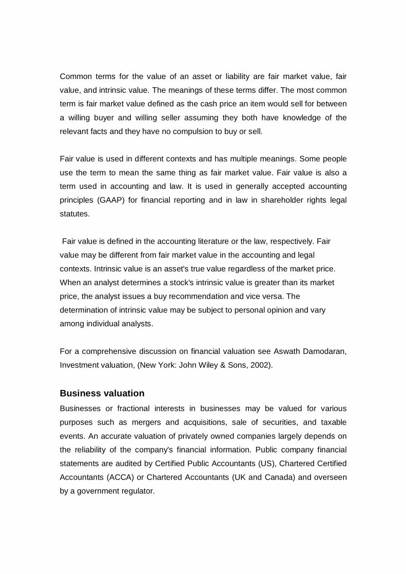
Common terms for the value of an asset or liability are fair market value, fair
value, and intrinsic value. The meanings of these terms differ. The most common
term is fair market value defined as the cash price an item would sell for between
a willing buyer and willing seller assuming they both have knowledge of the
relevant facts and they have no compulsion to buy or sell.
Fair value is used in different contexts and has multiple meanings. Some people
use the term to mean the same thing as fair market value. Fair value is also a
term used in accounting and law. It is used in generally accepted accounting
principles (GAAP) for financial reporting and in law in shareholder rights legal
statutes.
Fair value is defined in the accounting literature or the law, respectively. Fair
value may be different from fair market value in the accounting and legal
contexts. Intrinsic value is an asset's true value regardless of the market price.
When an analyst determines a stock's intrinsic value is greater than its market
price, the analyst issues a buy recommendation and vice versa. The
determination of intrinsic value may be subject to personal opinion and vary
among individual analysts.
For a comprehensive discussion on financial valuation see Aswath Damodaran,
Investment valuation, (New York: John Wiley & Sons, 2002).
Business valuation Businesses or fractional interests in businesses may be valued for various
purposes such as mergers and acquisitions, sale of securities, and taxable
events. An accurate valuation of privately owned companies largely depends on
the reliability of the company's financial information. Public company financial
statements are audited by Certified Public Accountants (US), Chartered Certified
Accountants (ACCA) or Chartered Accountants (UK and Canada) and overseen
by a government regulator.

Private companies do not have government oversight and are generally not
required to have their financial statements audited. private company financial
statements are commonly prepared to minimize taxes by lowering taxable
income and the financial information may not be accurate.
Public companies tend to want higher earnings to increase their share prices.
Inaccurate financial information can lead to over- and undervaluation. In an
acquisition, due diligence is commonly performed by the buyer to validate the
representations made by the seller.
Financial statements prepared in accordance with generally accepted accounting
principles (GAAP) usually express the values of the assets at their costs rather
than their higher market values. For example, the balance sheet would reflect a
piece of land at the purchase price rather than its appreciated value.
Certain types of assets and liabilities such as securities held for sale will be
reflected at their market values rather than their costs so that the company's
financial information is more meaningful. This process is called "mark-to-market"
but is subject to manager bias that may be compensated more with higher
values. An extreme example of a company taking advantage of mark-to-market
accounting to pump their own share price was Enron.
Business valuation methods
Discounted cash flows method This is a method used to determine the current value of a company using future
cash flows adjusted for time value. The future cash flows are the cash flows
within the determined forecast period and a continuing value that represents a
steady state cash flow stream after the forecast period is known as terminal
value.

Multiples method A method for determining the current value of a company by using a sample of
ratios from comparable peer groups the specific ratio to be used depends on the
objective of the valuation. The valuation could be designed to estimate the value
of the operation of the business or the value of the equity of the business.
In calculating the value of the operation the most commonly used ratio is the
EBITDA multiple. The ratio of EBITDA (earnings before interest taxes
depreciation and amortization) to the enterprise value (equity value plus debt
value) would give the EBITDA multiple.
In valuing the equity of a company, the most widely used multiple is the price
earnings ratio (PER) of stocks in a similar industry. The ratio of stock price to
earnings per share of any public company would give the price earnings ratio
(PER). Using the sum of multiple PER improves reliability but it can still be
necessary to correct the PER for current market conditions.
See also
Business valuation standards
Usage
In finance, valuation analysis is required for many reasons including tax
assessment, wills and estates, divorce settlements, business analysis, and basic
bookkeeping and accounting. Since the value of things fluctuates over time,
valuations are at a specific date e.g., the end of the accounting quarter or year.
They may alternatively be mark-to-market estimates of the current value of
assets or liabilities as of this minute or this day for the purposes of managing
portfolios and associated financial risk (for example, within large financial firms
including investment banks and stockbrokers).

Some balance sheet items are much easier to value than others are. Publicly
traded stocks and bonds have prices that are quoted frequently and readily
available. Other assets are harder to value. For instance, private firms that have
no frequently quoted price. Additionally, financial instruments that have prices
that are partly dependent on theoretical models of one kind or another are
difficult to value.
For example, options are generally valued using the Black-Scholes model while
the liabilities of life assurance firms are valued using the theory of present value.
Intangible business assets, like goodwill and intellectual property, are open to a
wide range of value interpretations.
It is possible and conventional for financial professionals to make their own
estimates of the valuations of assets or liabilities in that they are interested. Their
calculations are of various kinds including analyses of companies that focus on
price-to-book, price-to-earnings, price-to-cash flow and present value
calculations, and analyses of bonds that focus on credit ratings, assessments of
default risk, risk premium and levels of real interest rates.
All of these approaches may be thought of as creating estimates of value that
compete for credibility with the prevailing share or bond prices, where applicable,
and may or may not result in buying or selling by market participants. Where the
valuation is for the purpose of a merger or acquisition, the respective businesses
make available further detailed financial information, usually on the completion of
a non-disclosure agreement.
It is very important to note that valuation is more an art than a science because it
requires judgement:
1. There are very different situations and purposes in which you value an
asset (e.g. company in distress, tax purposes, mergers & acquisitions,

quarterly reporting). In turn, this requires different methods or a different
interpretation of the same method each time.
2. All valuation models and methods have their limitations (e.g.,
mathematical, complexity, simplicity, comparability) and could be widely
criticize able. As a rule, the valuation models are most useful when you
use the same valuation method as with the partner you are interacting.
Mostly the method used is industry or purpose specific;
3. The quality of some of the input data may vary widely
4. In all valuation, models there are a great number of assumptions that need
to be made and things might not turn out the way you expect. Your best
way out of that is to be able to explain and stand for each assumption you
make;
When a valuation is prepared all assumptions should be clearly stated, especially
the context. It is improper, for example, to value a going concern, based on an
assumption that it is going out of business, since then only a salvage value
remains.
Valuation of mining projects In mining, valuation is the process of determining the value or worth of a mining
property. Mining valuations are sometimes required for IPO's, fairness opinions,
litigation, mergers & acquisitions and shareholder related matters.
In valuation of a mining project or mining property, fair market value is the
standard of value to be used. The CIMVal Standards are a recognised standard
for valuation of mining projects and is recognised by the Toronto Stock Exchange
(Venture). The standards spearheaded by Spence & Roscoe, stress the use of
the cost approach, market approach and the income approach, depending on the
stage of development of the mining property or project.
Asset pricing models See also Modern portfolio theory
Capital asset pricing model (CAPM)
Arbitrage pricing theory (APT)
Black-Scholes (for Options)
Related Material
Present value
Efficient market hypothesis
Equity investment
Investment management
Depreciation
Real estate appraisal
Market-based valuation
Stock valuation
Appraisal
Earnings response coefficient
(3) Capital asset pricing model From Wikipedia, the free encyclopaedia
The capital asset pricing model (CAPM) is used in finance to determine a
theoretically appropriate required rate of return (and thus the price if expected
cash flows can be estimated) of an asset, if that asset is to be added to an
already well-diversified portfolio, given that asset's non-diversifiable risk.
The CAPM formula takes into account the asset's sensitivity to non-diversifiable
risk (also known as systematic risk or market risk), in a number often referred to

as beta (β) in the financial industry, as well as the expected return of the market
and the expected return of a theoretical risk-free asset.
The model was introduced by Jack L.Treynor, William Sharpe, John Lintner and
Jan Mossin independently, building on the earlier work of Harry Markowitz on
diversification and modern portfolio theory. Sharpe received the Bank of Sweden
prize in economic sciences in memory of Alfred Nobel memorial prize (jointly with
Harry Markowitz and Merton Miller) for this contribution to the field of financial
economics.
The formula The CAPM is a model for pricing an individual security (asset) or a portfolio. For
individual security perspective, we made use of the security market line (SML)
and its relation to expected return and systematic risk (beta) to show how the
market must price individual securities in relation to their security risk class.
The SML enables to calculate the reward-to-risk ratio for any security in relation
to that of the overall market. Therefore, when the expected rate of return for any
security is deflated by its beta coefficient, the reward-to-risk ratio for any
individual security in the market is equal to the market reward-to-risk ratio, thus:
Individual security’s / beta = Market’s securities (portfolio)
Reward-to-risk ratio Reward-to-risk ratio
E(Ri) - Rf \ βim = E(Rm) - Rf ,
The market reward-to-risk ratio is effectively the market risk premium and by
rearranging the above equation and solving for E(Ri), we obtain the capital asset
pricing model (CAPM).
E(Ri) = Rf + βim (E(Rm) - Rf).

Where:
E(Ri) is the expected return on the capital asset
Rf is the risk-free rate of interest
βim (the beta coefficient) the sensitivity of the asset returns to market
returns, or also
βim = Cov(Ri,Rm) \ Var(Rm),
E(Rm) is the expected return of the market
E(Rm)-Rf is sometimes known as the ''market premium'' or ''risk premium''
(the difference between the expected market rate of return and the risk-
free rate of return).
Note 1: the expected market rate of return is usually measured by looking
at the arithmetic average of the historical returns on a market portfolio (i.e.
S&P 500).
Note 2: the risk free rate of return used for determining the risk premium is
usually the arithmetic average of historical risk free rates of return and not
the current risk free rate of return.
For the full derivation, see Modern portfolio theory.
Asset pricing Once the expected return, E(Ri), is calculated using capital asset pricing model
(CAPM), the future cash flows of the asset can be discounted to their present
value using this rate (E(Ri)), to establish the correct price for the asset.
In theory, therefore, an asset is correctly priced when its observed price is the
same as its value calculated using the capital asset pricing model (CAPM)
derived discount rate. If the observed price is higher than the valuation, then the
asset is overvalued (and undervalued when the observed price is below the
CAPM valuation).

Alternatively, one can solve for the discount rate for the observed price given a
particular valuation model and compare that discount rate with the capital asset
pricing model (CAPM) rate. If the discount rate in the model is lower than the
capital asset pricing model (CAPM) rate then the asset is overvalued (and
undervalued for a too high discount rate).
Asset-specific required return The capital asset pricing model (CAPM) returns the asset-appropriate required
return or discount rate - i.e. the rate at which future cash flows produced by the
asset should be discounted given that asset's relative riskiness. Betas exceeding
one signify more than average riskiness; betas below one indicate lower than
average.
Thus, more risky stocks have a higher beta and will have to be discounted at a
higher rate; less sensitive stocks have lower betas and have to be discounted at
a lower rate. The capital asset pricing model (CAPM) is consistent with intuition -
investors (should) require a higher return for holding a more risky asset.
Since beta reflects asset-specific sensitivity to non-diversifiable, i.e. market risk,
the market as a whole, by definition, has a beta of one. Stock market indices are
frequently used as local proxies for the market - and in that case (by definition)
have a beta of one. An investor in a large, diversified portfolio (such as a mutual
fund) therefore expects performance in line with the market.
Risk and diversification The risk of a portfolio comprises systemic risk and specific risk, which is also
known an idiosyncratic risk. Systemic risk refers to the risk common to all
securities - i.e. market risk. Specific risk is the risk associated with individual
assets. Specific risk can be diversified away to smaller levels by including a
greater number of assets in the portfolio (specific risks ‘average out’); systematic
risk (within one market) cannot.
Depending on the market, a portfolio of approximately 30-40 securities in
developed markets such as UK or US (more in case of developing markets
because of higher asset volatilities) will render the portfolio sufficiently diversified
to limit exposure to systemic risk only.
A rational investor should not take on any diversifiable risk, as only non-
diversifiable risks are rewarded within the scope of this model. Therefore, the
required return on an asset, that is, the return that compensates for risk taken,
must be linked to its riskiness in a portfolio context - i.e. its contribution to overall
portfolio riskiness - as opposed to its stand-alone riskiness. In the CAPM context,
portfolio risk is represented by higher variance i.e. less predictability. In other
words, the beta of the portfolio is the defining factor in rewarding the systemic
exposure taken by an investor.
The efficient frontier The CAPM assumes that the risk-return profile of a portfolio can be optimised -
an optimal portfolio displays the lowest possible level of risk for its level of return.
Additionally, since each additional asset introduced into a portfolio further
diversifies the portfolio, the optimal portfolio must comprise every asset,
(assuming no trading costs) with each asset value-weighted to achieve the above
(assuming that any asset is infinitely divisible).
All such optimal portfolios, i.e., one for each level of return, comprise the efficient
frontier. Because the un-sys-tem-ice risk is diversifiable, the total risk of a
portfolio can be viewed as beta.
The market portfolio An investor might choose to invest a proportion of his or her wealth in a portfolio
of risky assets with the remainder in cash - earning interest at the risk free rate
(or indeed may borrow money to fund his or her purchase of risky assets in which

case there is negative cash weighting). Here, the ratio of risky assets to risk free
asset does not determine overall return - this relationship is clearly linear.
It is thus possible to achieve a particular return in one of two ways:
1. By investing all of one's wealth in a risky portfolio,
2. alternatively, by investing a proportion in a risky portfolio and the
remainder in cash (either borrowed or invested)
For a given level of return, however, only one of these portfolios will be optimal
(in the sense of lowest risk). Since the risk free asset is, by definition,
uncorrelated with any other asset, option 2 will generally have the lower variance
and hence be the more efficient of the two.
This relationship also holds for portfolios along the efficient frontier: a higher
return portfolio plus cash is more efficient than a lower return portfolio alone for
that lower level of return. For a given risk free rate, there is only one optimal
portfolio which can be combined with cash to achieve the lowest level of risk for
any possible return. This is the market portfolio.
Assumptions of CAPM All investors have rational expectations.
There are no arbitrage opportunities.
Returns are distributed normally.
Fixed quantity of assets
Perfectly efficient capital markets
Investors are solely concerned with level and uncertainty of future wealth
Separation of financial and production sectors
Thus, production plans are fixed.
Risk-free rates exist with limitless borrowing capacity and universal
access.
The Risk-free borrowing and lending rates are equal.

No inflation and no change in the level of interest rate exist.
Perfect information, hence all investors have the same expectations about
security returns for any given time period.
Shortcomings of CAPM The model assumes that asset returns are (jointly) normally distributed
random variables. It is however frequently observed that returns in equity
and other markets are not normally distributed. As a result, large swings
(between three to six standard deviations from the mean) occur in the
market more frequently than the normal distribution assumption would
expect.
The model assumes that the variance of returns is an adequate
measurement of risk. This might be justified under the assumption of
normally distributed returns, but for general return distributions, other risk
measures (like coherent risk measures) will likely reflect the investors'
preferences more adequately.
The model does not appear to explain the variation in stock returns.
Empirical studies show that low beta stocks may offer higher returns than
the model would predict. Some data to this effect was presented as early
as a 1969 conference in Buffalo, New York in a paper by Fischer Black,
Michael Jensen, and Myron Scholes. Either that fact is itself rational
(which saves the efficient markets hypothesis but makes CAPM wrong), or
it is irrational (which saves CAPM, but makes EMH wrong – indeed, this
possibility makes volatility arbitrage a strategy for reliably beating the
market).
The model assumes those given a certain expected return investors will
prefer lower risk (lower variance) to higher risk and conversely given a
certain level of risk will prefer higher returns to lower ones. It does not
allow for investors who will accept lower returns for higher risk. Casino

gamblers clearly pay for risk, and it is possible that some stock traders will
pay for risk as well.
The model assumes that all investors have access to the same
information and agree about the risk and expected return of all assets.
(Homogeneous expectations assumption)
The model assumes that there are no taxes or transaction costs, although
this assumption may be relaxed with complicated versions of the model.
The market portfolio consists of all assets in all markets, where each asset
is weighted by its market capitalization. This assumes no preference
between markets and assets for individual investors, and that investors
choose assets solely as a function of their risk-return profile. It also
assumes that all assets are infinitely divisible as to the amount, which may
be held or transacted.
The market portfolio theory should include all types of assets that are held
by anyone as an investment (including works of art, real estate, human
capital...) in practice, such a market portfolio is unobservable and people
usually substitute a stock index as a proxy for the true market portfolio.
Unfortunately, it has been shown that this substitution is harmful and can
lead to false inferences as to the validity of the capital asset pricing model
(CAPM), and it has been said that because of the inability to observe the
true market portfolio, the capital asset pricing model (CAPM) might not be
empirically testable. This was presented in greater depth in a paper by
Richard Roll in 1977, and was generally referred to as Roll's critique.
Theories such as the arbitrage pricing theory (APT) have since been
formulated to circumvent this problem.
Because CAPM prices a stock in terms of all stocks and bonds, it is really
an arbitrage-pricing model, which throws no light on how a firm's beta gets
determined.
Finding related topics

Valuation
Modern portfolio theory
Arbitrage pricing theory (APT)
Efficient market hypothesis
Earnings response coefficient
References Fama, E. and French, K. (1992) The cross-section of expected stock
returns, journal of finance, June 1992, 427-466.
Black, F., Jensen, M., and Scholes, M The capital asset pricing model:
some empirical tests, in M. Jensen ed., studies in the theory of capital
markets. (1972)
French, C. W. (2003). The Treynor capital asset pricing model, journal of
investment management, 1 (2), 60-72
Lintner, J. (1965). The valuation of risk assets and the selection of risky
investments in stock portfolios and capital budgets, Review of economics
and statistics, 47 (1), 13-37
Markowitz, Harry M. (1999). The early history of portfolio theory: 1600-
1960, Financial analysts journal, 55 (4)
Mossin, Jan. (1966). Equilibrium in a capital asset market, Econometrica,
34, 768-783
Ross, Stephen A. (1977). The capital asset pricing model (CAPM), short-
sale restrictions and related issues, Journal of finance, 32 (177)
Sharpe, William F. (1964). Capital asset prices: A theory of market
equilibrium under conditions of risk, Journal of finance, 19 (3), 425-442
Tobin, James (1958). Liquidity preference as behaviour towards risk, The
review of economic studies, 25
Treynor, J. L. (1961). Market value, time, and risk, unpublished manuscript
Treynor, J. L. (1962). Toward a theory of market value of risky assets
unpublished manuscript. A final version was published in 1999, in asset
pricing and portfolio performance: models, strategy and performance
metrics. Robert A. Korajczyk (editor) London: risk books, pp. 15-22
External links
Two asset efficient frontier
(http://www.duke.edu/~charvey/twoasset/index.html)
multiasset efficient frontier
(http://www.duke.edu/~charvey/frontier/frontier.html)
Fin Portfolio, free calculator allows five assets (http://www.finportfolio.edu)
Categories: Finance theories / Mathematical finance / Financial markets
(4) Arbitrage pricing theory From Wikipedia, the free encyclopaedia
Arbitrage pricing theory (APT), in Finance, is a general theory of asset pricing
that has become influential in the pricing of shares.
Arbitrage pricing theory (APT) holds that the expected return of a financial asset
can be modelled as a linear function of various macro-economic factors or
theoretical market indices, where sensitivity to changes in each factor is
represented by a factor specific beta coefficient. The model-derived rate of return
will then be used to price the asset correctly - the asset price should equal the
expected end of period price discounted at the rate implied by model. If the price
diverges, arbitrage should bring it back into line.
The theory was initiated by the economist Stephen Ross in 1976.

The arbitrage pricing theory (APT) model If arbitrage-pricing theory (APT) holds, then a risky asset can be described as
satisfying the following relation:
E(rj) = rf + bj1RP1 + bj2RP2 + ….. + bjnRPn
rj = E(rj) + bj1F1 + bj2F2 + ….. + bjnFn + εj
where
E(rj) is the risky asset's expected return,
RPk is the risk premium of the factor,
rf is the risk-free rate,
Fk is the macroeconomic factor,
bjk is the sensitivity of the asset to factor k, also called factor loading,
in addition, εj is the risky asset's idiosyncratic random shock with mean
zero.
That is, the uncertain return of an asset j is a linear relationship among n factors.
Additionally, every factor is also considered a random variable with mean zero.
Note that there are some assumptions and requirements that have to be fulfilled
for the latter to be correct: There must be perfect competition in the market, and
the total number of factors may never surpass the total number of assets (in
order to avoid the problem of matrix singularity),
Arbitrage and the arbitrage pricing theory (APT) Arbitrage is the practice of taking advantage of a state of imbalance between two
(or possibly more) markets and thereby making a risk free profit- see rational
pricing.

Arbitrage in expectations The arbitrage pricing theory (APT) describes the mechanism whereby arbitrage
by investors will bring an asset, which is wrongly priced, according to the
arbitrage pricing theory (APT) model, back into line with its expected price. Note
that under true arbitrage, the investor locks-in a guaranteed payoff, whereas
under arbitrage pricing theory (APT) arbitrage as described below, the investor
locks-in a positive expected payoff. The arbitrage pricing theory (APT) thus
assumes arbitrage in expectations - i.e. that arbitrage by investors will bring
asset prices back into line with the returns expected by the model portfolio
theory.
Arbitrage mechanics In the arbitrage pricing theory (APT) context, arbitrage consists of trading in two
assets - with at least one is being mispriced. The arbitrageur sells the asset,
which is relatively too expensive and uses the proceeds to buy one, which is
relatively too cheap.
Under the arbitrage pricing theory (APT), an asset is mispriced if its current price
diverges from the price predicted by the model. The asset price today should
equal the sum of all future cash flows discounted at the arbitrage pricing theory
(APT) rate, where the expected return of the asset is a linear function of various
factors, and sensitivity to changes in each factor is represented by a factor-
specific beta coefficient.
A correctly priced asset here may be in fact a synthetic asset - a portfolio
consisting of other correctly priced assets. This portfolio has the same exposure
to each of the macroeconomic factors as the mispriced asset. The arbitrageur
creates the portfolio by identifying x correctly priced assets (one per factor plus
one) and then weighting the assets such that portfolio beta per factor is the same
as for the mispriced asset.

When the investor is long the asset and short the portfolio (or vice versa) he has
created a position which has a positive expected return (the difference between
asset return and portfolio return) and which has a net-zero exposure to any
macroeconomic factor and is therefore risk free (other than for firm specific risk).
The arbitrageur is thus in a position to make a risk free profit:
Where today's price is too high:
The implication is that at the end of the period the portfolio would have
appreciated at the rate implied by the arbitrage pricing theory (APT), whereas the
mispriced asset would have appreciated at less than this rate. The arbitrageur
could therefore:
:: Today:
:::1 short sells the mispriced-asset
:::2 buy the portfolio with the proceeds.
:: At the end of the period:
:::1 sells the portfolio
:::2 use the proceeds to buy back the mispriced-asset
:::3 pocket the difference.
Relationship with the capital asset pricing model (CAPM) The arbitrage pricing theory (APT) along with the capital asset pricing model
(CAPM) is one of two influential theories on asset pricing. The arbitrage pricing
theory (APT) differs from the capital asset pricing model (CAPM) in that it is less
restrictive in its assumptions. It allows for an explanatory (as opposed to
statistical) model of asset returns.
It assumes that each investor will hold a unique portfolio with its own particular
array of betas, as opposed to the identical market portfolio. In some ways, the
capital asset pricing model (CAPM) can be considered a special case of the
arbitrage pricing theory (APT) in that the securities market line represents a

single-factor model of the asset price, where beta is exposure to changes in
value of the market.
Additionally, the arbitrage pricing theory (APT) can be seen as a supply side
model, since its beta coefficients reflect the sensitivity of the underlying asset to
economic factors. Thus, factor shocks would cause structural changes in the
asset's expected return, or in the case of stocks, in the firm's profitability.
On the other side, the capital asset pricing model (CAPM) is considered a
demand side model. Its results, although similar to those in the arbitrage pricing
theory (APT), arise from a maximization problem of each investor's utility
function, and from the resulting market equilibrium, (investors are considered the
consumers of the assets).
Using the arbitrage pricing theory (APT)
Identifying the factors As with the capital asset pricing model (CAPM), the factor-specific betas are
found via a linear regression of historical security returns on the factor in
question. Unlike the capital asset pricing model (CAPM), the arbitrage pricing
theory (APT), however, does not itself reveal the identity of its priced factors - the
number and nature of these factors is likely to change over time and between
economies. As a result, this issue is essentially empirical in nature.
Several a priori guidelines as to the characteristics required of potential factors,
however are suggested:
1. their impact on asset prices manifests in their unexpected movements
2. they should represent undiversifiable influences (these are, clearly, more
likely to be macroeconomic rather than firm-specific in nature)
3. timely and accurate information on these variables is required
4. the relationship should be theoretically justifiable on economic grounds

Chen, Roll and Ross identified the following macro-economic factors as
significant in explaining security returns:
surprises in inflation;
surprises in GNP as indicted by an industrial production index;
surprises in investor confidence due to changes in default premium in
corporate bonds;
surprise shifts in the yield curve.
As a practical matter, indices or spot or futures market prices may be used in
place of macro-economic factors, which are reported at low frequency (e.g.
monthly) and often with significant estimation errors. Market indices are
sometimes derived by means of factor analysis. Direct indices that might be
used are:
short term interest rates;
the difference in long-term and short term interest rates;
a diversified stock index such as the S&P 500 or NYSE Composite Index;
oil prices
gold or other precious metal prices
currency exchange rates
Arbitrage pricing theory (APT) and asset management See also
rational pricing
fundamental theorem of arbitrage-free pricing
capital asset pricing model
efficient market hypothesis
modern portfolio theory
earnings response coefficient
value investing
References Burmeister E and Wall KD., The arbitrage pricing theory and
macroeconomic factor measures, The Financial Review, 21:1-20, 1986
Chen, N.F, and Ingersoll, E., Exact pricing in linear factor models with
finitely many assets: A note, Journal of Finance June 1983
Roll, Richard and Stephen Ross, An empirical investigation of the
arbitrage pricing theory, Journal of Finance, Dec 1980,
Ross, Stephen, The arbitrage theory of capital asset pricing, Journal of
Economic Theory, v13, issue 3, 1976
External links
The arbitrage pricing theory
(http://viking.som.yale.edu/will/finman540/classnotes/class6.html) Prof.
William N. Goetzmann, Yale school of management
The arbitrage pricing theory approach to strategic portfolio planning
http://www.cfapubs.org/doi/pdf/10.2469/faj.v51.n1.1868 (PDF), Richard
Roll and Stephen A. Ross
The APT (http://www-
personal.umich.edu/~shumway/courses.dir/ba855.dir/apt.PDF) Prof.
Tyler Shumway, University of Michigan business school
The arbitrage pricing theory
(http://www.moneymax.co.za/articles/displayarticlewide.asp?ArticleID=27
3656), The investment analysts' society of South Africa
References on the arbitrage pricing theory
(http://www.kellogg.northwestern.edu/faculty/korajczy/htm/aptlist.htm),
Prof. Robert A. Korajczyk, Kellogg School of Management
Categories: Finance theories / Mathematical finance / Pricing / Financial
economics

(5) Terminal value From Wikipedia, the free encyclopaedia
In finance, the terminal value of a security is the present value at a future point in
time of all future cash flows when we expect stable growth rate forever. It is most
often used in multi-stage discounted cash flow analysis, and allow for the
limitation of cash flow projections to a several-year period. Forecasting results
beyond such a period is impractical and exposes such projections to a variety of
risks limiting their validity, primarily the great uncertainty involved in predicting
industry and macroeconomic conditions beyond a few years.
Thus, the terminal value allows for the inclusion of the value of future cash flows
occurring beyond a several-year projection period while satisfactorily mitigating
many of the problems of valuing such cash flows. The terminal value is
calculated in accordance with a stream of projected future free cash flows in
discounted cash flow analysis. For whole-company valuation purposes, there are
two methodologies used to calculate the terminal value.
Perpetuity Growth Model The perpetuity growth model accounts for the value of free cash flows that
continues into perpetuity in the future, growing at an assumed constant rate.
Here, the projected free cash flow in the first year beyond the projection horizon
(N+1) is used.
This value is divided by the discount rate minus the assumed perpetuity growth
rate: T(0) = FCF N+1 / (k - g). T(0) is the value of future cash flows at a future
point in time, which is immediately prior to N+1, or at the end of period N, which
is the final year in the projection period. This equation is a perpetuity, which uses
a geometric series to determine the value of a series of growing future cash
flows.
To determine the present value of the terminal value, one must discount the
terminal value at T(0) by a factor equal to the number of years included in the
initial projection period. If N is the 5th and final year in this period, then the
terminal value is divided by (1 + k)5 The present value of the terminal value is
then added to the PV of the free cash flows in the projection period to arrive at an
implied enterprise value.
Exit multiple approaches The exit or terminal multiple approaches assume a business will be sold at the
end of the projection period. Valuation analytics are determined for various
operating statistics using comparable acquisitions. A frequently used terminal
multiple is enterprise value / EBITDA.
The analysis of comparable acquisitions will indicate an appropriate range of
multiples to use. The multiple is then applied to the projected EBITDA in year n,
which is the final year in the projection period. This provides a future value at the
end of year n.
The terminal value is then discounted using a factor equal to the number of years
in the projection period. If n is the 5th and final year in this period, then the
terminal value is divided by (1 + k)5 The present value of the terminal value is
then added to the PV of the free cash flows in the projection period to arrive at an
implied enterprise value.
Note that if publicly traded comparable company multiples must be used, the
resulting implied enterprise value will not reflect a control premium. Depending
on the purposes of the valuation, this may not provide an appropriate reference
range.
Comparison of methodologies There are several important differences between the two approaches. The
perpetuity growth model has several inherent characteristics that make it
intellectually challenging. Because both the discount rate and growth rate are
assumptions, inaccuracies in one or both inputs can provide an improper value.
The difference between the two values in the denominator determines the
terminal value, and even with appropriate values for both, the denominator may
result in a multiplying effect that does not estimate an accurate terminal value.
In addition, the perpetuity growth rate assumes that free cash flow will continue
to grow at a constant rate into perpetuity. Consider that a perpetuity growth rate
exceeding the annualized growth of the S&P 500 and/or the U.S. GDP implies
that the company's cash flow will outpace and eventually absorb these rather
large values.
Perhaps the greatest disadvantage to the perpetuity growth model is that it lacks
the market-driven analytics employed in the exit multiple approach. Such
analytics result in a terminal value based on operating statistics present in a
proven market for similar transactions. This provides a certain level of confidence
that the valuation accurately depicts how the market would value the company in
reality.
On the other hand, the exit multiple approach must be used carefully, because
multiples change over time. Simply applying the current market multiple ignores
the possibility that current multiples may be high or low by historical standards.
In addition, it is important to note that at a given discount rate, any exit multiple
implies a terminal growth rate and conversely any terminal growth rate implies an
exit multiple. When using the exit multiple approach it is often helpful to calculate
the implied terminal growth rate, because a multiple that may appear reasonable
at first glance can actually imply a terminal growth rate that is unrealistic.
In practice, academics tend to use the perpetuity growth model, while investment
bankers favour the exit multiple approach. Ultimately, these methods are two

different ways of saying the same thing. For both terminal value approaches, it is
essential to use a range of appropriate discount rates, exit multiples and
perpetuity growth rates in order to establish a functional valuation range.
See also
terminal value (accounting)
geometric series
perpetuity
Categories: Basic financial concepts / Fundamental analysis
(6) Free cash flow From Wikipedia, the free encyclopaedia
Free cash flow measures a firm's net increase in
operating cash flow (this includes the reduction for interest),
less the dividends paid to preferred shareholders, and
less expenditures necessary to maintain assets (often referred to as
capital expenditures or Capex).
Increases in non-cash current assets may be deducted or not, depending on
whether they are considered to maintain the status quo, or to investments for
growth.
Uses of the metric Free cash flow measures the ease with which businesses can grow and pay
dividends to shareholders. Even profitable businesses may have negative cash
flows. Their requirement for increased financing will result in increased financing
costs reducing future income.

According to the discounted cash flow valuation model, the intrinsic value of a
company is the present value of all future free cash flows, plus the cash
proceeds from its eventual sale. The presumption is that the cash flows are used
to pay dividends to the shareholders.
Some investors prefer using free cash flow instead of net income to measure a
company's financial performance, because free cash flow is more difficult to
manipulate than net income. The problems with this presumption are itemized at
cash flow and return of capital.
The payout ratio is a metric used to evaluate the sustainability of distributions
from REITs, Oil & Gas Royalty Trusts, and Income Trust. The distributions are
divided by the free cash flow. Distributions may include any of income, flowed-
through capital gains or return of capital.
Problems with CapEx The expenditures for maintenance of assets are only part of the capital
expenditure (capex) reported on the statement of cash flows. It must be
separated from the expenditures for growth purposes. This split is not a
requirement under GAAP, and is not audited.
Management is free to disclose maintenance capital expenditure (capex) or not.
Therefore, this input to the calculation of free cash flow may be subject to
manipulation, or require estimation. Since it may be a large number,
maintenance capex's uncertainty is the basis for some people's dismissal of free
cash flow.
A second problem with the maintenance capital expenditure (capex)
measurement is its intrinsic lumpiness. By their nature, expenditures for capital
assets that will last decades may be infrequent, but costly when they occur. Free

cash flow, in turn, will be very different from year to year. No particular year will
be a norm that can be expected to be repeated. For companies that have stable
capital expenditures, free cash flow will be (over the long term) roughly equal to
earnings.
External links
Free cash flow: free, but not always easy
(http://www.investopedia.com/articles/fundamental/03/091703.asp),
Investopedia
What is free cash flow?
(http://news.morningstar.com/classroom2/course.asp?docId=2937&CN=C
OM&page=1&_QSBPA=Y), Morningstar
Categories: Management accounting / Business
(7) Discounted cash flow From Wikipedia, the free encyclopaedia
In finance, the discounted cash flow (or DCF) approach describes a method to
value a project or an entire company using the concepts of the time value of
money. All future cash flows are estimated and discounted to give them a
present value. The discount rate used is generally the appropriate cost of capital,
and incorporates judgments of the uncertainty (riskiness) of the future cash flows.
Discounted cash flow analysis is widely used in investment finance, real estate
development, and corporate financial management.
Mathematics The discounted cash flow (DCF) formula is derived from the future value formula
for calculating the time value of money and compounding returns.

FV = PV .* (1+d)n
The simplified version of the discounted cash flow (DCF) equation (for one cash
flow in one future period) is expressed as:
DPV = (FV / (1+d)n)
Where:
DPV is the discounted present value of the future cash flow (FV), or FV
adjusted for the opportunity cost of future receipts and risk of loss;
FV is the nominal value of a cash flow amount in a future period;
d is the discount rate, which is the opportunity cost plus risk factor (or the
time value of money: ‘I’ in the future-value equation);
n is the number of discounting periods used (the period in which the future
cash flow occurs). i.e. if the receipts occur at the end of year 1, n will be
equal to 1; at the end of year 2, 2—likewise, if the cash flow happens
instantly, n becomes 0, rendering the expression an identity (DPV=FV).
Where multiple cash flows in multiple times are discounted, it is necessary to
sum them as follows:
n
DPV = ∑ FVt / (1+d)t
t=0
For each future cash flow (FV) at any time (t) for all times The sum can then be
used as a net present value figure or used to calculate the internal rate of return
for a cash flow pattern over time.
Example DCF To show how discounted cash flow analysis is performed, consider the following
simplified example.

John Doe buys a house for $100,000. Three years later, he expects to be
able to sell this house for $150,000.
Simple subtraction suggests that the value of his profit on such a transaction
would be $150,000 - $100,000 = $50,000, or 50%. If that $50,000 were
amortized over the three years, his implied annual return (known as the internal
rate of return) would be about 13.6%. Looking at those figures, he might be
justified in thinking that the purchase looked like a good idea.
However, since three years have passed between the purchase and the sale,
any cash flow from the sale must be discounted accordingly.
At the time John Doe buys the house, the 3-year US treasury bill rate is
5%. Treasury bills are generally considered inherently less risky than real
estate, since the value of the Bill is guaranteed by the US government and
there is a liquid market for the purchase and sale of T-bills. If he had not
put his money into buying the house, he could have invested it in the
relatively safe T-bills instead. By not doing so, he has incurred an
opportunity cost from his decision.
Therefore, calculating exclusively for opportunity cost, we get a discount rate of
5% per year (taking the comparable-period Treasury rate of return directly).
Using the DPV formula above, that means that the value of $150,000 received in
three years actually has a present value of $129,576 (rounded off). Those future
dollars are not worth the same as the dollars we have now.
Subtracting the purchase price of the house ($100,000) from the present value
results in the net present value, which would be $29,576 or a little more than
29%? Amortized over the three years, that implies a discounted annual return of
8.6% (still very respectable, but only 63% of the profit he previously thought he

would have). Note that the original internal rate of return (13.6%) minus the
discount rate (5%) equals the discounted internal rate of return (8.6%). The
discount rate directly modifies the annual rate of return.
However, what about risk
The house John is buying is in a good neighbourhood, but market values
have been rising quite a lot lately and the real estate market analysts in
the media are talking about a slow-down and higher interest rates. There
is a probability that John might not be able to get the full $150,000 he is
expecting in three years due to a slowing of price appreciation, or that loss
of liquidity in the real estate market might make it very hard for him to sell
at all.
For the sake of the example, let us then estimate his risk factor is about 5% (we
could perform a more precise probabilistic analysis of the risk, but that is beyond
the scope of this article).Therefore, this analysis should now include both
opportunity cost (5%) and risk (5%), for a total discount rate of 10% per year.
Going back to the DPV formula, $150,000 received three years from now and
discounted at a rate of 10% is only worth $111,261 (rounded off) in present-day
dollars. The present-value profit on the sale is now down to $11,261 discounted
dollars from $50,000 nominal dollars. The implied annual rate of return on that
discounted profit is now 3.6% per year.
That return rate may seem low, but it is still positive after all of our discounting,
suggesting that the investment decision is probably a good one: it produces
enough profit to compensate for opportunity cost and risk with a little extra left
over. When investors and managers perform DCF analysis, the important thing
is that the net present value of the decision after discounting all future cash flows
at least be positive (more than zero).

If it is negative, that means that the investment decision would actually lose
money even it appears to generate a nominal profit. For instance, if the expected
sale price of John Doe's house in the example above was not $150,000 in three
years, but $130,000 in three years or $150,000 in five years, then buying the
house would actually cause John to lose money in present-value terms (about
$6,000 in the first case, and about $9,000 in the second).
Similarly, if the house was located in an undesirable neighbourhood and the
Federal reserve bank was about to raise interest rates by five percentage points,
then the risk factor would be a lot higher than 5%. It might not be possible for him
to make a profit in discounted terms even if he could sell the house for $200,000
in three years.
In this example, only one future cash flow was considered. For a decision, which
generates multiple cash flows in multiple times, discounted cash flow (DCF)
analysis must be performed on each cash flow in each period and summed into a
single net present value.
Methods Depending on the financing schedule of the company, four different DCF
methods are distinguished today. Since the underlying financing assumptions are
different, they do not need to arrive at the same value of the project or company:
equity-approach
Flows to equity approach (FTE)
entity-approach:
Adjusted present value approach (APV)
Weighted average cost of capital approach (WACC)
Total cash flow approach (TCF)
History Discounted cash flow calculations have been used in some form since money
was first lent at interest in ancient times. As a method of asset valuation, it has
often been opposed to accounting book value, which is based on the amount
paid for the asset. Following the stock market crash of 1929, discounted cash
flow analysis gained popularity as a valuation method for stocks. Irving Fisher in
his 1930 book ‘The Theory of Interest’ and John Burr William’s 1938 text 'The
Theory of Investment Value' first formally expressed the DCF method in modern
economic terms.
See also
adjusted present value
capital budgeting
economic value added
Flows to equity
net present value
valuation using discounted cash flows
time Value of Money
cost of capital
External links
Disk lectures [http://www.disklectures.com/freebies.php], discounted cash
flow audio lecture with slideshow
Great moments in financial economics [http://www.in-the-
money.com/pages/author.htm]
The theory of interest
[http://www.econlib.org/library/YPDBooks/Fisher/fshToI.html] at the Library
of Economics and Liberty [http://www.econlib.org/index.html]
Monograph about DCF (including some lectures on DCF)
[http://www.wacc.biz]
Foolish Use of DCF
[http://www.fool.com/news/commentary/2005/commentary05032803.htm]
Literature
Tom Copeland, Tim Koller, Jack Murrin: Valuation. J. Wiley & Sons, 2nd
edition, 1998
Categories: Basic financial concepts / Finance / Real estate
(8) Net present value From Wikipedia, the free encyclopaedia
Net present value (NPV) is a standard method for the financial appraisal of long-
term projects. Used for capital budgeting, and widely throughout economics, it
measures the excess or shortfall of cash flows, in present value (PV) terms, once
financing charges are met. By definition,
NPV = Present value of net cash flows. For its expression, see the formula
section below.
Formula Each cash inflow/outflow is discounted back to its PV. Then they are summed.
Therefore
n
NPV = ∑ Ct / (1+r)t - C0
t=1
Where:
t - the time of the cash flow
n - the total time of the project

r - the discount rate
Ct - the net cash flow (the amount of cash) at time t.
C0 - the capital outlay at the beginning of the investment time ( t = 0 )
For more information on how to calculate the present value (PV) of a dollar or of
a stream of payments, see time value of money.
The discount rate Choosing an appropriate discount rate is crucial to the net present value (NPV)
calculation. A good practice of choosing the discount rate is to decide the rate,
which the capital needed for the project, could return if invested in an alternative
venture. If, for example, the capital required for project A can earn five percent
elsewhere, use this discount rate in the net present value (NPV) calculation to
allow a direct comparison to be made between project A and the alternative.
Obviously, net present value (NPV) value obtained using variable discount rates
with the years of the investment duration is more reflecting to the real situation
than that calculated from a constant discount rate for the entire investment
duration. Refer to the tutorial article written by Samuel Baker1for more detailed
relationship between the net present value (NPV) value and the discount rate.
For some professional investors, their investment funds are committed to target a
specified rate of return. In such cases, that rate of return should be selected as
the discount rate for the net present value (NPV) calculation. In this way, a direct
comparison can be made between the profitability of the project and the desired
rate of return.
The rate used to discount future cash flows to their present values is a key input
of this process. Most firms have a well-defined policy regarding their capital
structure. Therefore, the weighted average cost of capital (after tax) is
appropriate for use with all projects. Alternately, higher discount rates can be

used for more risky projects. Another method is to apply higher discount rates to
cash flows occurring further along the time span, to reflect the yield curve
premium for long-term debt.
Reinvestment rate There are assumptions made about what rate of return is realized on cash that is
freed-up before the end of the project. In the net present value (NPV) model, it is
assumed to be reinvested at the discount rate used. This is appropriate in the
absence of capital rationing.
In the IRR model, no assumption is made about the reinvestment rate of free
cash, which tends to exaggerate the calculated values. Some people believe that
if the firm's reinvestment rate is higher than the weighted average cost of capital,
it would be in effect, an opportunity cost and should be used as the discount rate.
What NPV tells With a particular project, if Ct is a positive value, the project is in the status of
cash inflow in the time of t. If Ct is a negative value, the project is in the status of
cash outflow in the time of t. Appropriately, risked projects with a positive net
present value (NPV) should be accepted. This does not necessarily mean that
they should be undertaken since net present value (NPV) at the cost of capital
may not account for opportunity cost, i.e. comparison with other available
investments. In financial theory, if there is a choice between two mutually
exclusive alternatives, the one yielding the higher net present value (NPV) should
be selected. The following sums up the net present value’s (NPV) various
situations.

If... It means... Then…
NPV > 0 the investment would the project should be accepted
add value to the firm
NPV < 0 the investment would the project should be rejected
subtract value from
the firm
NPV = 0 the investment would the project could be accepted
neither gain nor lose because shareholders obtain
value for the firm required rate of return. This project
adds no monetary value. Decision
should be based on other criteria,
e.g.
strategic positioning or other factors
not
explicitly included in the calculation.
Example X corporation must decide whether to introduce a new product line. The new
product will have start-up costs, operational costs, and incoming cash flows over
six years.
This project will have an immediate (t=0) cash outflow of $100,000 (which might
include machinery, and employee training costs). Other cash outflows for years
1-6 are expected to be $5,000 per year. Cash inflows are expected to be $30,000
per year for years 1-6. All cash flows are after-tax, and there are no cash flows
expected after year 6. The required rate of return is 10%.
The present value (PV) can be calculated for each year:

t=0 -$100,000 / 1.100 = -$100,000 PV.
t=1 ($30,000 - $5,000)/ 1.101 = $22,727 PV.
t=2 ($30,000 - $5,000)/ 1.102 = $20,661 PV.
t=3 ($30,000 - $5,000)/ 1.103 = $18,783 PV.
t=4 ($30,000 - $5,000)/ 1.104 = $17,075 PV.
t=5 ($30,000 - $5,000)/ 1.105 = $15,523 PV.
t=6 ($30,000 - $5,000)/ 1.106 = $14,112 PV.
The sum of all these present values is the net present value (NPV), which equals
$8,882. Since the net present value (NPV) is greater than zero, the corporation
should invest in the project.
Problems that are more realistic would need to consider other factors, generally
including the calculation of taxes, uneven cash flows, and salvage values as well
as the availability of alternate investment opportunities.
Common Pitfalls If some (or all) of the Ct have a negative value, then paradoxical results are
possible. For example, if the Ct are generally negative late in the project (eg, an
industrial or mining project might have clean up and restoration costs), then an
increase in the discount rate can make the project appear more favourable.
Some people see this as a problem with net present value (NPV). A way to avoid
this problem is to include explicit provision for financing any losses after the initial
investment, i.e., explicitly calculate the cost of financing such losses.
Another common pitfall is to adjust for risk by adding a premium to the discount
rate. Whilst a bank might charge a higher rate of interest for a risky project, that
does not mean that this is a valid approach to adjusting a net present value for
risk, although it can be a reasonable approximation in some specific cases.
One reason such an approach may not work well can be seen from the
foregoing: if some risk is incurred resulting in some losses, then a discount rate
in the net present value (NPV) will reduce the impact of such losses below their
true financial cost. A rigorous approach to risk requires identifying and valuing
risks explicitly, e.g. by actuarial or Monte Carlo techniques, and explicitly
calculating the cost of financing any losses incurred.
Yet another issue can result from the compounding of the risk premium. R is a
composite of the risk free rate and the risk premium. As a result, future cash
flows are discounted by the risk free rate as well as the risk premium and this
effect is compounded by each subsequent cash flow. This compounding results
in a much lower net present value (NPV) than might be otherwise calculated. The
certainty equivalent model can be used to account for the risk premium without
compounding its effect on present value.
Influence of currency system Currency systems that include demurrage alter the effective cost of capital and
lead to an increased net present value (NPV) emphasis on long-term returns.
While such currency systems are untypical in the modern world, they were
prevalent in earlier eras when commodities formed the basis of private
currencies.
Alternative capital budgeting methods payback period: which measures the time required for the cash inflows to
equal the original outlay? It measures risk, not return.
cost-benefit analysis : which includes issues other than cash, such as
timesaving?
real option method : which attempts to value managerial flexibility that is
assumed away in net present value (NPV)?
internal rate of return (IRR): which calculates the rate of return of a project
without making assumptions about the reinvestment of the cash flows
(hence internal)
modified internal rate of return (MIRR) - similar to Internal rate of return,
but it makes explicit assumptions about the reinvestment of the cash
flows. Sometimes called Growth Rate of Return
Applications of NPV NPV Methodology, Examples, Limitations
[http://www.odellion.com/pages/online%20community/NPV/financialmodel
s_npv_definition.htm ].
Using NPV to calculate share prices [http://www.advanced-
excel.com/net_present_value.html].
Calculating Net Present Value [http://www.alvinhan.com/NPV-IRR.htm]
See also
rate of return on investment
capital budgeting
cost of capital
discounted cash flow
internal rate of return
real versus nominal value
References Baker, Samuel L. (2000). Perils of the Internal Rate of Return
(http://hspm.sph.sc.edu/COURSES/ECON/investment.html)
Categories: Basic financial concepts / Mathematical finance / Investment

(9) Enterprise value From Wikipedia, the free encyclopaedia
Enterprise value (EV), total enterprise value (TEV), or firm value (FV) is a market
value measure of a company from the point of view of the aggregate of all the
financing sources; debt holders, preferred shareholders, minority shareholders
and common equity holders. Because enterprise value (EV) is a capital
structure-neutral metric, it is useful when comparing companies with diverse
capital structures.
Enterprise value = Common equity at equity value
+ debt at market value
+ minority interest at market value, if any
+ preferred equity at market value
- cash and cash-equivalents.
Cash is subtracted because when it is paid out as a dividend, it reduces the net
cost to the purchaser. Therefore, the business was only worth the reduced
amount to start with. The same effect is accomplished when the cash is used to
pay down debt.
Metrics using enterprise value (EV) EBITDA is the measure of cash returns that accrue to all the shareholders in
aggregate. The corresponding measure of income would be Net Income with the
after-tax cost of interest backed out.
EV/EBITDA is the metric most used to measure how many years it would
take to payback the investment. This metric is equivalent to the payback
period used by debt holders (debt/EBITDA). The P/E metric used by
shareholders is similar except it measures earnings, not cash flow.
EBITDA/EV is the metric most used to measure the cash rate of return on
the investment.

Usage Stock market investors use EBITDA/EV to compare returns between equivalent
companies on a risk-adjusted basis. They can then impose their own choice of
personal debt levels. In practice, stock investors cannot use enterprise value
(EV) because they have no access to the market values of the company debt.
It is not sufficient to substitute the book value of the debt because a) the market
interest rates may have changed, and b) the market's perception of the risk of the
loan may have changed since the debt was issued. Remember, the point of
enterprise value (EV) is to neutralize the different risks, and costs of different
capital structures.
Buyers of controlling interests in a business use enterprise value (EV) to
compare returns between businesses, as above. They also use the EV valuation
to determine how much to pay for the whole entity (not just the equity). They
may want to change the capital structure once in control.
External links
Investopedia: Enterprise Value
[http://www.investopedia.com/terms/e/enterprisevalue.asp]
Categories: Mathematical finance / Fundamental analysis / Economics and
finance stubs
(10) Weighted average cost of capital From Wikipedia, the free encyclopaedia
The weighted average cost of capital (WACC) is used in finance to measure a
firm's cost of capital. This has been used by many firms in the past as a discount
rate for financed projects, as the cost of financing (capital) is regarded by some
as a logical discount rate (required rate of return) to use.

Corporations raise money from two main sources: equity and debt. Thus, the
capital structure of a firm comprises three main components: preferred equity,
common equity and debt (typically bonds and notes). The WACC takes into
account the relative weights of each component of the capital structure and
presents the expected cost of new capital for a firm.
The formula The weighted average cost of capital is defined by:
c = (E \ K) y + (D \ K) b (1-tC)
where:
K = D + E
in addition, the following table defines each symbol:
Symbol Meaning Units
c weighted average cost of capital %
y required or expected rate of return on equity, or cost of equity %
b required or expected rate of return on borrowings, or cost of debt %
tC corporate tax rate %
D total debt and leases currency
E total equity and equity equivalents currency
K total capital invested in the going concern currency
This equation describes only the situation with homogeneous equity and debt. If
part of the capital consists, for example, of preferred stock (with different cost of
equity (y), then the formula would include an additional term for each additional
source of capital.

How it works Since we are measuring expected cost of new capital, we should use the market
values of the components, rather than their book values (which can be
significantly different). In addition, other, more exotic sources of financing, such
as convertible/callable bonds, convertible preferred stock, etc., would normally be
included in the formula if they exist in any significant amounts - since the cost of
those, financing methods is usually different from the plain vanilla bonds and
equity due to their extra features.
Sources of information How do we find out the values of the components in the formula for WACC?
First, let us note that the weight of a source of financing is simply the market
value of that piece divided by the sum of the values of all the pieces. For
example, the weight of common equity in the above formula would be determined
as follows:
Market value of common equity / (Market value of common equity + Market value
of debt + Market value of preferred equity)
Find the market values of each source of financing (namely the debt, preferred
stock, and common stock)
The market value for equity for a publicly traded company is simply the
price per share multiplied by the number of shares outstanding, and tends
to be the easiest component to calculate.
The market value of debt can be easily found if the company has publicly
traded bonds. Frequently, companies also have a significant amount of
bank loans, whose market value is not easily found. However, since the
market value of debt tends to be pretty close to the book value (for
companies that have not experienced significant changes in credit rating,
at least), the book value of debt is usually used in the WACC formula.

The market value of preferred stock is again usually easily found on the
market, and determined by multiplying the cost per share by number of
shares outstanding.
Preferred equity is equivalent to perpetuity, where the holder is entitled to fixed
payments forever. Thus, the cost is determined by dividing the periodic payment
by the price of the preferred stock, in percentage terms.
The cost of common equity is usually determined using the capital asset pricing
model.
The cost of debt is the yield to maturity on the publicly traded bonds of the
company. Failing availability of that, the rates of interest charged by the banks on
recent loans to the company would also serve as a good cost of debt. Since a
corporation normally can write off taxes on the interest it pays on the debt,
however, the cost of debt is further reduced by the relevant tax rate of the
corporation.
Thus, the cost of debt for a company becomes (YTM on bonds or interest on
loans) x (1 - tax rate). In fact, the tax deduction is usually kept in the formula for
WACC, rather than being rolled up into cost of debt, as such:
WACC = weight of preferred equity x cost of preferred equity
+ weight of common equity x cost of common equity
+ weight of debt x cost of debt x (1 - tax rate)
Now we are ready to plug all our data into the WACC formula.

Effect on valuation The economists Merton Miller and Franco Modigliani showed in the Modigliani-
Miller theorem that in a perfect economy without taxes, a firm's cost of capital
(and thus the valuation) does not depend on the debt to equity ratio. However,
many governments allow a tax deduction on interest and thus in such an
environment, there is a bias towards debt financing.
References G. Bennet Stewart III The Quest for Value, HarperCollins
M. Miller and F. Modigliani: Corporate income taxes and the cost of
capital: a correction American Economic Review, 53 (3) (1963), pp. 433-
443
J. Miles und J. Ezzell: The weighted average cost of capital, perfect capital
markets and project life: a clarification. Journal of Financial and
Quantitative Analysis, 15 (1980), S. 719-730.
See also
Cost of capital
Modigliani-Miller theorem
Video about practical application of the WACC approach
[http://www.wacc.de/index.htm#Example]
Category: Capital
External links
Information Quality and Cost of Capital
[http://papers.ssrn.com/sol3/papers.cfm?abstract_id=846546]
Ignacio Vélez-Pareja, Politécnico Grancolombiano - Department of
Business Management and Joseph Tham, Duke University - Duke Center
for International Development in the Sanford Institute of Public Policy;

Duke University - Center for Health Policy, Law and Management A Note
on the Weighted Average Cost of Capital WACC
[http://papers.ssrn.com/sol3/papers.cfm?abstract_id=254587] Solving the
Circularity Problem
Calculate the WACC with your own values to understand the equation
[http://formularium.org/?go=96]
(11) Business value From Wikipedia, the free encyclopaedia
In management, business value is an informal term that includes all forms of
value that determine the health and well-being of the firm in the end. Business
value expands concept of value of the firm beyond economic value (also known
as economic profit, economic value added, and shareholder value) to include
other forms of value such as employee value, customer value, supplier value,
channel partner value, alliance partner value, managerial value, and societal
value. Many of these forms of value are not directly measured in monetary terms.
Business value often embraces intangible assets not necessarily attributable to
any stakeholder group. Examples include intellectual capital and a firm's
business model. The Balanced scorecard methodology is one of the most
popular methods for measuring and managing business value.
Philosophy The concept of business value aligned with the theory that a firm is best viewed
as a network of relationships both internal and external. These networks are
sometimes called a value network or value chain. Each node in the network
could be a stakeholder group, a resource, an organization, end-consumers,
interest groups, regulators, or the environment itself. In a value network, value
creation is viewed as a collaborative, creative, synergistic processes rather than
purely mechanistic or a result of command-and-control.
If the firm is viewed as a network of value creating entities, then the question
becomes how each node in the network does contribute to overall firm
performance and how does it behave and respond to its own interests. When the
nodes are independent organizations (e.g. suppliers) or agents (e.g. customers),
it is assumed that the firm is seeking a cooperative, win-win relationship where all
parties receive value. Even when nodes in the network are partially independent
(e.g. employees), it is assumed that incentives are important and that those
incentives go beyond direct financial compensation.
While it would be very desirable to translate all forms of business value to a
single economic measure (e.g. discounted cash flow), many practitioners and
theorists, believe this is either not feasible or theoretically impossible. Therefore,
advocates of business value believe that the best approach is to measure and
manage multiple forms of value as they apply to each stakeholder group.
Yet, there are no well-formed theories about how the various elements of
business value are related to each other and how they might contribute to the
firm's long-term success. One promising approach is the business model, but
these are rarely formalized.
History Peter Drucker was an early proponent of business value as the proper goal of a
firm, especially that a firm should create value for customers, employees
(especially knowledge workers), and distribution partners. His management by
objectives was a goal setting and decision-making tool to help managers at all
levels create business value. However, he was sceptical that the dynamics of
business value could ever be formalized, at least not with current methods.

Michael Porter popularized the concept of value chain.
Components of business value Shareholder value For a publicly traded company, shareholder value is the part of its capitalization
that is equity as opposed to long-term debt. In the case of only one type of stock,
this would roughly be the number of outstanding shares times current share
price. Things like dividends augment shareholder value while issuing of shares
(stock options) lower it. This Shareholder value added should be compared to
average/required increase in value, also known as cost of capital.
For a privately held company, the value of the firm after debt must be estimated
using one of several valuation methods, discounted cash flow or others.
See Shareholder value
Customer value Customer value is the value received by the end-customer of a product or
service. End-customer can include a single individual (consumer) or an
organization with various individuals playing different roles in the
buying/consumption processes. Customer value is conceived variously as utility,
quality, benefits, and customer satisfaction.
See customer value and utility
Employee value
Channel partner value
Supplier value
Managerial value
Societal value

Strategies for creating business value An increase or decline in business value that an action produces is traditionally
measured in terms of customer satisfaction, revenue growth, and profitability,
market share, and wallet share, cross-sell ratio, marketing campaign response
rates or relationship duration.
Business value of information technology Various factors affect the business value impact of information technology
(IT).The most important factor is the alignment between IT and business
processes, organization structure, and strategy. At the highest levels, this
alignment is achieved through proper integration of enterprise architecture,
business architecture, process design, organization design, and performance
metrics.
At the level of computing and communications infrastructure, the following
performance factors constrain and partially determine IT capabilities:
usability
functionality
availability
reliability, recoverability
performance (throughput, response time, predictability, capacity, etc)
security
agility
In extreme programming, the goal of delivering incremental business value drives
each iteration of development.
Criticisms Business value is an informal concept and there is no consensus, either in
academic circles or among management professionals, on its meaning or role in
effective decision-making. The term could even be described as a buzzword
used by various consultants, analyst firms, executives, authors, and academics.
Some critics believe that measuring economic value, economic profit, or
shareholder value is sufficiently complete to guide decision-making. Their logic
is that all other forms of value are essentially intermediate to the ultimate goal of
economic profit. Furthermore, if they do not contribute to economic profit, they
are actually a distraction for the firm.
Other critics believe that extensive efforts to measure business value will be
more of a distraction than a boon. For example, there is a fear that decision-
makers will be confused if there are too many goals and measures that need to
be accommodated
Categories: Management/ Organizational theory/ financial economics
(12) Stock valuation From Wikipedia, the free encyclopaedia
There are several methods used to value companies and their stocks. They
attempt to give an estimate of their fair value, by using fundamental economic
criteria. This theoretical valuation has to be perfected with market criteria, as the
final purpose is to determine potential market prices.
Fundamental criteria (fair value) The most theoretically sound valuation method of stock is called income
valuation or the discounted cash flow (DCF) method, involving discounting the
profits (dividends, earnings, or cash flows) the stock will bring to the stockholder
in the near future, and a final value on disposition. The discount rate normally

has to include a risk premium, which is commonly based on the capital asset
pricing model.
The Gordon model or Gordon's growth model1is the best known of a class of
discounted dividend models It assumes that dividends will increase at a constant
growth rate (less than the discount rate) forever The valuation is given by the
formula:
n
P = D . ∑_({1+g}/{1+k})i = D . {1+g}/{k-g} .
i=1
in addition, the following table defines each symbol:
Symbol Meaning Units
P estimated stock price $ or € or pound
D last dividend paid $ or € or pound
k discount rate %
g the growth rate of the dividends %
1[http://www.fool.co.uk/qualiport/2000/qualiport000628.htm]
The P/E method is perhaps the most commonly used valuation method in the
stock brokerage industry. By using comparison firms, a target price/earnings (or
P/E) ratio is selected for the company, and then the future earnings of the
company are estimated. The valuation's fair price is simply estimated earnings
times target P/E. This model is essentially the same model as Gordon's model, if
k-g is estimated as the dividend payout ratio (D/E) divided by the target P/E ratio.
Market criteria (potential price) Some feel that if the stock is listed in a well-organized stock market, with a large
volume of transactions, the listed price will be close to the estimated fair value.
This is called the efficient market hypothesis.

On the other hand, studies made in the field of behavioural finance tend to show
that deviations from the fair price are rather common, and sometimes quite large.
Thus, in addition to fundamental economic criteria, market criteria also have to
be taken into account market-based valuation. Valuing a stock is not only to
estimate its fair value, but also to determine its potential price range, taking into
account the aspects of market behaviour. One of the behavioural valuation tools
is the stock image, a coefficient that bridges the theoretical fair value and the
market price and it is good for everyone.
See also
stock picking
list of valuation topics
capital asset pricing model
value at risk
fundamental analysis
technical analysis
fed model Theory of Equity Valuation
External links
Development of the PE Valuation Method
[http://www.investingator.org/PEND-stock-investing.html]
MIT Open Course Ware [http://ocw.mit.edu/OcwWeb/Sloan-School-of-
Management/15-414Financial-
ManagementSummer2003/LectureNotes/index.htm]

(13) Fundamental analysis From Wikipedia, the free encyclopaedia
Fundamental analysis of a business involves analyzing its financial statements
and health, its management and competitive advantages, and its competitors and
markets. The analysis is performed on historical and present data, but with the
goal to make financial projections. There are several possible objectives:
to calculate a company's credit risk,
to make projection on its business performance,
to evaluate its management and make internal business decisions,
to make the company's stock valuation and predict its probable price
evolution
Two analytical models When the objective of the analysis is to determine what stock to buy and at what
price, there are two basic methodologies.
1. Fundamental analysis maintains that markets may misprice a security in
the short run but that the correct price will eventually be reached. Profits
can be made by trading the mispriced security and then waiting for the
market to recognise its mistake and re-price the security.
2. Technical analysis maintains that all information is reflected already in the
stock price, so fundamental analysis is a waste of time. Trends are your
friend and sentiment changes predate and predict trend changes.
Investors' emotional responses to price movements lead to recognizable
price chart patterns. Technical analysis does not care what the value of a
stock is. Their price predictions are only extrapolations from historical
price patterns.
Investors can use both these different but somewhat complementary methods for
stock picking. Many fundamental investors use technical for deciding entry and

exit points. Many technical investors use fundamentals to limit their universe of
possible stock to good companies.
The choice of stock analysis is determined by the investor's belief in the different
paradigms for how the stock market works. See the discussions at efficient
market hypothesis, random walk hypothesis, capital asset pricing model, Fed
model theory of equity valuation, and behavioural finance.
Use by different portfolio styles Investors may use fundamental analysis within different portfolio management
styles.
Buy and hold investors believe that latching onto good businesses allows
the investor's asset to grow with the business. Fundamental analysis lets
them find good companies, so they lower their risk and probability of wipe
out.
Managers may use fundamental analysis to value correctly good and bad
companies. Even bad company's stock goes up and down, creating
opportunities for profits.
Contrarian investors distinguish in the short run, the market is a voting
machine, not a weighing machine. Fundamental analysis allows you to
make your own decision on value, and ignore the market.
Value investors restrict their attention to under-valued companies,
believing that it is hard to fall out of a ditch. The value comes from
fundamental analysis.
Managers may use fundamental analysis to determine future growth rates
for buying high priced growth stocks.
Managers may also include fundamental factors along with technical
factors into computer models (quantitative analysis).
Top-down and Bottom-up Investors can either use a top-down or bottom-up approach.
The top-down investor starts his analysis with global economics, including
both international and national economic indicators, such as GDP growth
rates, inflation, interest rates, exchange rates, productivity, and energy
prices. He narrows his search down to regional/industry analysis of total
sales, price levels, the effects of competing products, foreign competition,
and entry or exit from the industry. Only then does he narrow his search to
the best business in that area.
The bottom-up investor starts with specific businesses, regardless of their
industry/region.
Procedures
The analysis of a business' health starts with financial statement analysis that
includes ratios. It looks at dividends paid, operating cash flow, new equity issues
and capital financing. The earnings estimates and growth rate projections
published widely by Thomson Financial and others can be considered either
fundamental (they are facts) or technical (they are investor sentiment) based on
your perception of their validity.
The determined growth rates (of income and cash) and risk levels (to determine
the discount rate) are used in various valuation models. The foremost is the
discounted cash flow model, which calculates the present value of the future
Dividends received by the investor, along with the eventual sale price.
(Gordon model)
earnings of the company, or
Cash flows of the company.
The simple model commonly used is the price/earnings ratio. Implicit in this
model of a perpetual annuity (time value of money) is that the flip of the P/E is

the discount rate appropriate to the risk of the business. The multiple accepted is
adjusted for expected growth (that is not built into the model).
Growth estimates are incorporated into the PEG ratio but the math does not hold
up to analysis. Its validity depends on the length of time you think the growth will
continue.
Computer modelling of stock prices has now replaced much of the subjective
interpretation of fundamental data (along with technical data) in the industry.
Since about year 2000, vast quantities of data were crunched with the power of
computers and a new career had been invented. At some funds, the manager's
decisions have been replaced by proprietary mathematical models.
Criticisms
Some economists such as Burton Malkiel suggest that neither
fundamental analysis nor technical analysis is useful in outperforming the
markets. [http://www.investopedia.com/university/concepts/concepts5.asp
Financial concepts: Random Walk Theory]
See also
list of valuation topics
stock picking
security Analysis
External links
Comprehensive fundamental data on all UK listed companies
[http://www.hemscott.com]
MIT open course ware [http://ocw.mit.edu/OcwWeb/Sloan-School-of-
Management/15-414Financial-
ManagementSummer2003/LectureNotes/index.htm]

Procedures for stock picking - 4 pages
[http://members.shaw.ca/RetailInvestor/next.html]
Development of the PEND Method [http://www.investingator.org/PEND-
stock-investing.html]
Fundamental analysis Lens [http://www.squidoo.com/fundamental-
analysis]
Fundamental analysis [http://www.thestreet.com/financial-
dictionary/fundamental-analysis.html]
(14) Stochastic modelling From Wikipedia, the free encyclopaedia
Stochastic model Stochastic means being or having a random variable. A stochastic model is a tool
for estimating probability distributions of potential outcomes by allowing for
random variation in one or more inputs over time. The random variation is usually
based on fluctuations observed in historical data for a selected period using
standard time-series techniques. Distributions of potential outcomes are derived
from a large number of simulations (stochastic projections) which reflect the
random variation in the input(s).
Its application initially started in physics (sometimes known as the Monte Carlo
Method). It is now being applied in life sciences and social science, especially
finance.
See also economic capital
Valuation Like any other company, an insurer has to show that its assets exceed its
liabilities to be solvent. In the insurance industry, however, assets and liabilities
are not known entities. They depend on how many policies result in claims,

inflation from now until the claim, investment returns during that period, and so
on.
Therefore, the valuation of an insurer involves a set of projections, looking at
what is expected to happen, and thus coming up with the best estimate for
assets and liabilities, and therefore for the company's level of solvency.
Deterministic approach The easiest way of doing this, and indeed the method which has been the
primary one used, is to look at best estimates.
The projections should use the most likely rate of claim, the most likely
investment return, the most likely rate of inflation, and so on. This creates a point
estimate - the best single estimate of what the company's current solvency
position is.
The downside of this approach is it ignores the fact that there is uncertainty in the
estimates, and that a whole range of outcomes is possible. It is all very well to
know what is most likely, but we are also interested in what range of outcomes
are probable.
Stochastic modelling A stochastic model would be to set up a projection model, which looks at a single
policy, an entire portfolio or an entire company. Rather than setting investment
returns according to their most likely estimate, for example, the model uses
random variations to look at what investment conditions might be like.
Based on a set of random outcomes, the experience of the
policy/portfolio/company is projected, and the outcome is noted. Then this is
done again with a new set of random variables. In fact, this process is repeated
thousands of times.

At the end, a distribution of outcomes is available which shows not only what the
most likely estimate, but what ranges are reasonable too.
This is useful when a policy or fund provides a guarantee, e.g. a minimum
investment return of 5% per annum. A deterministic simulation, with varying
scenarios for future investment return, does not provide a good way of estimating
the cost of providing this guarantee.
This is because it does not allow for the volatility of investment returns in each
future time or the chance that an extreme event in a particular time leads to an
investment returns less than the guarantee. Stochastic modelling builds volatility
and variability (randomness) into the simulation and therefore provides a more
accurate representation of real life.
Numerical evaluations of quantities Stochastic models help to assess the interactions between variables, and are
useful tools to evaluate numerically quantities, as they are usually implemented
using Monte Carlo simulation techniques (see Monte Carlo method). While there
is an advantage here, in estimating quantities that would otherwise be difficult to
obtain using analytical methods, a disadvantage is that such methods are limited
by computing resources as well as simulation error. Below are some examples:
Means
Using statistical notation, it is a well-known result that the mean of a function, f, of
a random variable X is not necessarily the function of the mean of X.
For example, in application, applying the best estimate (defined as the mean) of
investment returns to discount a set of cash flows will not necessarily give the
same result as assessing the best estimate to the discounted cash flows.
A stochastic model would be able to assess this latter quantity with simulations.

Percentiles This idea is seen again, when one considers percentiles (see percentile). When
assessing risks at specific percentiles, the factors that contribute to these levels
are rarely at these percentiles themselves. Stochastic models can be simulated
to assess the percentiles of the aggregated distributions.
Truncations and censors
Truncating and censoring of data can also be estimated using stochastic models.
For instance, applying a non-proportional reinsurance layer to the best estimate
losses will not necessarily give us the best estimate of the losses after the
reinsurance layer. In a simulated stochastic model, the simulated losses can be
made to pass through the layer and the resulting losses assessed appropriately.
The asset model Although the text above referred to random variations, the stochastic model does
not just use any arbitrary set of values. The asset model is based on detailed
studies of how markets behave, looking at averages, variations, correlations, and
more.
The models and underlying parameters are chosen so that they fit historical
economic data, and are expected to produce meaningful future projections.
There are many such models, including the Willkie model, the Thompson model
and the Falcon model.
The Claims model The claims arising from policies or portfolios that the company has written can
also be modelled using stochastic methods. This is especially important in the
general insurance sector, where the claim severities can have high uncertainties.
Frequency-severity models Depending on the portfolios under investigation, a model can simulate all or
some of the following factors stochastically:
number of claims
claim severities
timing of claims
Claims inflations can be applied, based on the inflation simulations that are
consistent with the outputs of the asset model, as are dependencies between the
losses of different portfolios.
The relative uniqueness of the policy portfolios written by a company in the
general insurance sector means that claims models are typically tailor-made.
Stochastic reserving models Estimating future claims liabilities might also involve estimating the uncertainty
around the estimates of claim reserves.
See J Li's article 'Comparison of Stochastic Reserving Models’ (published in the
Australian Actuarial Journal, volume 12 issue 4) for a recent article on this topic
References
Basic Stochastic Processes [http://www.amazon.co.uk/Basic-Stochastic-
Processes-Undergraduate-Mathematics/dp/3540761756] (book)
Options, Futures & Other Derivatives [http://www.amazon.co.uk/Options-
Futures-Other-Derivatives-International/dp/0130465925] (book)
Stochastic Models for Actuarial Use
[http://www.assa.org.za/scripts/file_build.asp?id=100000654] (pdf)
Guidance on stochastic modelling for life insurance reserving
[http://www.actuaries.org.uk/files/pdf/life_insurance/GN47notes_20050902
.pdf] (pdf)
J Li's article on stochastic reserving from the Australian Actuarial Journal,
2006
[http://www.actuaries.asn.au/IAA/upload/public/Vol12_Issue4(web).pdf]
(pdf)
Categories: Actuarial science/ Financial terminology/ Statistical randomness
15) Equity investment From Wikipedia, the free encyclopaedia
Equity investment generally refers to the buying and holding of shares of stock
on a stock market by individuals and funds in anticipation of income from
dividends and capital gain as the value of the stock rises. It also sometimes
refers to the acquisition of equity (ownership) participation in a private (unlisted)
company or a start-up (a company being created or newly created). When the
investment is in infant companies, it is referred to as venture capital investing and
is generally understood to be higher risk than investment in listed going-concern
situations.
Direct holdings and pooled funds The equities held by private individuals are often held via mutual funds or other
forms of pooled investment vehicle, many of which have quoted prices that are
listed in financial newspapers or magazines; the mutual funds are typically
managed by prominent fund management firms (e.g. Fidelity or Vanguard). Such
holdings allow individual investors to obtain the diversification of the fund(s) and
to obtain the skill of the professional fund managers in charge of the fund(s).
An alternative usually employed by large private investors and institutions (e.g.
large pension funds) is to hold shares directly; in the institutional environment
many clients that own portfolios have what are called segregated funds as
opposed to, or in addition to, the pooled e.g. mutual fund alternative.

Pros and cons The major advantages of investing in pooled funds are access to professional
investor skills and obtaining the diversification of the holdings within the fund.
The investor also receives the services associated with the fund e.g. regular
written reports and dividend payments (where applicable). The major
disadvantages of investing in pooled funds are the fees payable to the managers
of the fund (usually payable on entry and annually and sometimes on exit) and
the diversification of the fund that may or may not be appropriate given the
investors circumstances.
It is possible to over-diversify. If an investor holds several funds, then the risks
and structure of his overall position is an amalgam of the holdings in all the
different funds and arguably, the investor’s holdings successively approximate to
an index or market risk.
The costs or fees paid to the professional fund management organisation need to
be monitored carefully. In the worst cases, the costs (e.g. fees and other costs
that may be less obvious hidden fees within the workings of the investing
organisation) are large relative to the dividend income payable on the stock
market and to the total post-tax return that the investor can anticipate in an
average year.
Analysis
To try to identify good shares to invest in, two main schools of thought exist:
technical analysis and fundamental analysis. The former involves the study of
the price history of a share(s) and the price history of the stock market as a
whole; technical analysts have developed an array of indicators, some very
complex, that seek to tease useful information from the price and volume series.
Fundamental analysis involves study of all pertinent information relevant to the
stock and market in question in an attempt to forecast future business and

financial developments including the likely trajectory of the share price(s) itself.
The fundamental information studied will include the annual report and accounts,
industry data (such as sales and order trends) and study of the financial and
economic environment (e.g. the trend of interest rates).
Share price determination Ultimately, at any given moment, equity’s price is strictly a result of supply and
demand. The supply is the number of shares offered for sale at any one moment.
The demand is the number of shares investors wish to buy at exactly that same
time. The price of the stock moves in order to achieve and maintain equilibrium.
When buyers outnumber sellers, the price rises. Eventually sellers enter, and/or
buyers leave, achieving equilibrium between buyers and sellers. When sellers
outnumber buyers, the price falls. Eventually buyers enter, and/or sellers leave,
again achieving equilibrium.
Thus, what a share of a company at any given moment is determined by all
investors voting with their money. If more investors want a stock and are willing
to pay more, the price will go up. If more investors are selling a stock and there
are not enough buyers, the price will go down.
Of course, that does not explain how people decide the maximum price at which
they are willing to buy or the minimum at which they are willing to sell. In
professional investment circles, the efficient markets hypothesis (EMH) continues
to be popular, although this theory is widely discredited in academic and
professional circles.
Briefly, efficient markets hypothesis (EMH) says that investing is rational; that the
price of a stock at any given moment represents a rational evaluation of the
known information that might bear on the future value of the company. The share
prices of equities are priced efficiently, which is to say that they represent
accurately the expected value of the stock, as best it can be known at a given
moment. In other words, prices are the result of discounting expected future cash
flows.
The efficient markets hypothesis (EMH) model, if true, has to at least two
interesting consequences. First, because financial risk is presumed to require at
least a small premium on expected value, the return on equity can be expected
to be slightly greater than that available from non-equity investments. If not, the
same rational calculations would lead equity investors to shift to these safer non-
equity investments that could be expected to give the same or better return at
lower risk.
Second, because the price of a share at every given moment is an efficient
reflection of expected value, then relative to the curve of expected return-prices
will tend to follow a random walk, determined by the emergence of news
(randomly) over time. Professional equity investors therefore immerse
themselves in the flow of fundamental information. They seek to gain an
advantage over their competitors (mainly other professional investors) by more
intelligently interpreting the emerging flow of information (news).
The efficient markets hypothesis (EMH) model does not seem to give a complete
description of the process of equity price determination. For example, stock
markets are more volatile than efficient markets hypothesis (EMH) would imply.
In recent years, it has come to be accepted that the share markets are not
perfectly efficient, perhaps especially in emerging markets or other markets that
are not dominated by well-informed professional investors.
Another theory of share price determination comes from the field of behavioural
finance. According to behavioural finance, humans often make irrational
decisions-particularly, related to the buying and selling of securities-based upon
fears and misperceptions of outcomes. The irrational trading of securities can
often create securities prices, which vary from rational, fundamental price
valuations.
For instance, during the technology bubble of the late 1990s (which was followed
by the dot-com bust of 2000-2002), technology companies were often bid beyond
any rational fundamental value because of what is commonly known as the
greater fool theory. The greater fool theory holds that, because the predominant
method of realizing returns in equity is from the sale to another investor, one
should select securities that they believe that someone else will value at a higher
level at some point in the future, without regard to the basis for that other party's
willingness to pay a higher price. Thus, even a rational investor may rely on
others' irrationality.
See also
Investment management
Stock investor
Stock valuation
References
Chapter 12 of the General Theory of Employment Interest and Money, by
John Maynard Keynes (Author), 1936
Yes, You Can Time the Market!, by Ben Stein (Author), Phil DeMuth
(Author), John Wiley & Sons, 2003, hardcover, 240 pages, ISBN 0-471-
43016-1
The Profit Magic of Stock Transaction Timing, J.M.Hurst (Author),
Prentice-Hall, 1970
Security Analysis: Principles and Techniques (Second Edition), Benjamin
Graham and David Dodd (Authors); (a classic study of how to analyse
companies prior to investment)
External links
Stock Market Investing (http://www.hemscott.com/markets.do)
Financial Times Equities News (http://news.ft.com/markets/equities)
Equities Org (http://equities.org.uk/)
Forbes Equity Headlines (http://www.forbes.com/equities/)
16) Cost-benefit analysis From Wikipedia, the free encyclopaedia
Cost-benefit analysis is a term that refers:
a formal discipline used to help appraise, or assess, the case for a project
or proposal, which itself is a process known as project appraisal; and
An informal approach to making decisions of any kind
Under both definitions, the process involves, whether explicitly or implicitly,
weighing the total expected costs against the total expected benefits of one or
more actions in order to choose the best or most profitable option. The formal
process is often referred to as cost-benefit analysis (CBA), or benefit-cost
analysis in the United States.
Closely related, but slightly different, formal techniques include cost-effectiveness
analysis and benefit effectiveness analysis.
Theory Cost benefit Analysis is an economic tool to aid social decision-making, and is
typically used by governments to evaluate the desirability of a given intervention
in markets. The aim is to gauge the efficiency of the intervention relative to the
status quo. The costs and benefits of the impacts of an intervention are
evaluated in terms of the public's willingness to pay for them (benefits) or
willingness to pay to avoid them (costs).

Inputs are typically measured in terms of opportunity costs - the value in their
best alternative use. The guiding principle is to list all of the parties affected by an
intervention, and place a monetary value of the effect it has on their welfare as it
would be valued by them.
The process involves monetary value of initial and ongoing expenses vs.
expected return. Constructing plausible measures of the costs and benefits of
specific actions is often very difficult. In practice, analysts try to estimate costs
and benefits either by using survey methods or by drawing inferences from
market behaviour.
For example, a product manager may compare manufacturing and marketing
expenses to projected sales for a proposed product, and only decide to produce
it if he expects the revenues eventually to recoup the costs. Cost-benefit analysis
attempts to put all relevant costs and benefits on a common temporal footing.
A discount rate is chosen, which is then used to compute all relevant future costs
and benefits in present-value terms. Most commonly, the discount rate used for
present-value calculations is an interest rate taken from financial markets (R.H.
Frank 2000). This can be very controversial - for example, a high discount rate
implies a very low value on the welfare of future generations, which may have a
huge impact on the desirability of interventions to help the environment, and so
on. Empirical studies have suggested that in reality, peoples' discount rates do
decline over time. Because CBA aims to measure the public's true willingness to
pay, this feature is typically built into studies.
During cost-benefit analysis, monetary values may also be assigned to less
tangible effects such as the various risks which could contribute to partial or total
project failure; loss of reputation, market penetration, long-term enterprise
strategy alignments, etc. This is especially true when governments use the

technique, for instance to decide whether to introduce business regulation, build
a new road or offer a new drug on the state healthcare.
A value must be put on human life or the environment, often causing great
controversy. The cost-benefit principle says, for example, that we should install a
guardrail on a dangerous stretch of mountain road if the dollar cost of doing so is
less than the implicit dollar value of the injuries, deaths, and property damage
thus prevented (R.H. Frank 2000).
Cost-benefit calculations typically involve using time value of money formula.
This is usually done by converting the future expected streams of costs and
benefits to a present value amount.
Application Cost-benefit analysis is mainly, but not exclusively, used to assess the value for
money of very large private and public sector projects. This is because such
projects tend to include costs and benefits that are less amenable to being
expressed in financial or monetary terms (e.g. environmental damage), as well
as those that can be expressed in monetary terms. Private sector organisations
tend to make much more use of other project appraisal techniques, such as rate
of return, where feasible.
The practice of cost-benefit analysis differs between countries and between
sectors (e.g. transport, health) within countries. Some of the main differences
include the types of impacts that are included as costs and benefits within
appraisals, the extent to which impacts are expressed in monetary terms and
differences in discount rate between countries.
Transport The most sophisticated application of cost-benefit analysis is in the transport
sector.

UK Basic cost-benefit techniques were applied to the development of the motorway
network in the 1950s and 60s. An early, and often quoted, more developed
application of the technique was made to London underground's Victoria line.
Over the last 40 years, cost-benefit techniques have gradually developed to the
extent that substantial guidance now exists on how transport projects should be
appraised in the UK. The department for transport (DfT) and its agencies have
made extensive use of a number of key cost-benefit indicators, including:
PVB (present value of benefits);
PVC (present value of costs);
NPV (PVB less PVC);
NPV/k (where k is the level of funds available); and
BCR (benefit cost ratio).
In 1998, the new approach to appraisal (NATA) was introduced by the then
department for transport, environment and the regions. This brought together
cost-benefit results with those from detailed environmental impact assessments
and presented them in a balanced way. NATA was first applied to national road
schemes in the 1998 roads review, but subsequently rolled out to all modes of
transport. It is now a cornerstone of transport appraisal in the UK and is
maintained and developed by the department for transport.
EU The EU's developing harmonised European approaches for transport costing and
project assessment (HEATCO) project, part of its sixth framework programme,
has reviewed transport appraisal guidance across EU member states and found
that significant differences exist between countries. HEATCO's aim is to develop
guidelines to harmonise transport appraisal practice across the EU. (1)
[http://heatco.ier.uni-stuttgart.de/]

US Much of the early development work on cost-benefit analysis as a discipline was
the result of problems faced by the US Army Corps of Engineers in deciding how
and where to build bridges in supporting combat operations.
Benefit-cost analysis is now a well-established discipline in the US. California's
department of transportation (Caltrans) provide detailed guidance on how
benefit-cost analysis should be applied to transport projects.
Accuracy problems
The accuracy of the outcome of a cost-benefit analysis is dependent on how
accurately costs and benefits have been estimated. A peer-reviewed study (2)
[http://flyvbjerg.plan.aau.dk/JAPAASPUBLISHED.pdf] of the accuracy of cost
estimates in transportation infrastructure planning found that for rail projects
actual costs turned out to be on average 44.7 percent higher than estimated
costs, and for roads 20.4 percent higher (Flyvbjerg, Holm, and Buhl, 2002).
For benefits, another peer-reviewed study (3)
[http://flyvbjerg.plan.aau.dk/Traffic91PRINTJAPA.pdf] found that actual rail
ridership was on average 51.4 percent lower than estimated ridership; for roads it
was found that for half of all projects estimated traffic was wrong by more than 20
percent (Flyvbjerg, Holm, and Buhl, 2005). Comparative studies indicate that
similar inaccuracies apply to fields other than transportation. These studies
indicate that the outcomes of cost-benefit analyses should be treated with
caution, because they may be highly inaccurate.
In fact, inaccurate cost-benefit analyses may be argued to be a substantial risk in
planning, because inaccuracies of the size documented are likely to lead to
inefficient decisions, as defined by Pareto and Kaldor-Hicks efficiency (4)
[http://books.google.com/books?vid=ISBN0521009464&id=RAV5P-

50UjEC&printsec=toc&dq=flyvbjerg] Flyvbjerg, Bruzelius, and Rothengatter,
2003).
These outcomes (usually tending to underestimation, unless significant new
approaches are overlooked) are to be expected, since such estimates:
1. rely heavily on past like projects (frequently differing markedly in function or
size, and certainly in the skill levels of the team members),
2. rely heavily on the project's members to identify (remember from their
collective past experiences) the significant cost drivers,
3. rely on very crude heuristics (rules of thumb) to estimate the money cost of the
intangible elements, and
4. are unable to completely dispel the usually (unconscious) biases of the team
members (who often have a vested interest in a decision to go ahead) and the
natural psychological tendency to think positive (whatever that involves).
Another challenge to cost-benefit analysis comes from determining which costs
should be included in an analysis (the significant cost drivers). This is often
controversial as organizations or interest groups may feel that some costs should
be included or excluded from a study.
In the case of the Ford Pinto (where, due to design flaws, the Pinto was liable to
burst into flames in a rear-impact collision), the Ford company's decision was not
to issue a recall. Ford's cost benefit analysis had estimated that: based on the
number of cars in use and the probable accident rate, deaths due to the design
flaw would run about $49.5 million (the amount Ford would pay out of court to
settle wrongful death lawsuits).
This was estimated to be less than the cost of issuing a recall ($137.5 million) (5)
[http://www.safetyforum.com/fordfuelfires/]. In the event, Ford overlooked (or
considered insignificant) the costs of the negative publicity so engendered, which

turned out to be quite significant (since it led to the recall anyways and to
measurable losses in sales).
Sources and further reading
Bent Flyvbjerg, Nils Bruzelius, and Werner Rothengatter, Megaprojects
and Risk: An Anatomy of Ambition (Cambridge University Press,
2003).[http://books.google.com/books?vid=ISBN0521009464&id=RAV5P-
50UjEC&printsec=toc&dq=flyvbjerg]
Bent Flyvbjerg, Mette K. Skamris Holm, and Søren L. Buhl,
Underestimating costs in public works projects: error or lie. Journal of the
American Planning Association, vol. 68, no. 3, Summer 2002, pp. 279-
295. [http://flyvbjerg.plan.aau.dk/JAPAASPUBLISHED.pdf]
Bent Flyvbjerg, Mette K. Skamris Holm, and Søren L. Buhl, How (In)
accurate are Demand Forecasts in Public Works Projects The Case of
Transportation Journal of the American Planning Association, vol. 71, no.
2, Spring 2005, pp. 131-146.
[http://flyvbjerg.plan.aau.dk/Traffic91PRINTJAPA.pdf]
Tevfik F. Nas, Cost-Benefit Analysis: Theory and Application (Thousand
Oaks, Ca.: Sage, 1996).
[http://books.google.com/books?vid=ISBN0803971338&id=wttV6nAtdMkC
&pg=PP1&lpg=PP7&dq=%22cost+benefit+analysis%22&sig=oA2-
XuXSydPNvjjM29YvgxACil8]
See also
Kaldor-Hicks efficiency - economic principle underlying cost-benefit
analysis
Net present value - a similar type of calculation
Optimism bias
Parametric estimating - cost estimating methodology
Pareto efficiency - alternative economic principle

Risk-benefit analysis - in many decisions, such as in bio-medical research,
the cost is replaced by risk
External links
(10) [http://www.costbenefitanalysis.org] - The Environmental Valuation &
Cost-Benefit Website
(11) [http://www.envirovaluation.org] - Environmental Valuation & Cost-
Benefit News
(12) [http://www.dot.ca.gov/hq/tpp/offices/ote/Benefit_Cost/index.html] -
Caltrans Guide to Benefit-Cost Analysis
(13) [http://flyvbjerg.plan.aau.dk/JAPAASPUBLISHED.pdf] - Inaccuracy in
cost estimates
(14) [http://flyvbjerg.plan.aau.dk/Traffic91PRINTJAPA.pdf] - Inaccuracy in
benefit estimates
Decision Analysis in Health Care
(http://gunston.gmu.edu/healthscience/730/default.asp) George Mason
University online course offering lectures and tools for measuring cost-
effectiveness in health care scenarios
Cost-Benefit Analysis [http://www.informatics-
review.com/wiki/index.php/Cost-Benefit_Analysis_(CBA)] on Clinfowiki
17) Interest rate swap From Wikipedia, the free encyclopaedia
In the field of derivatives, a popular form of swap is the interest rate swap, in
which one party exchanges a stream of interest for another party's stream.
These were originally created to allow multi-national companies to evade
exchange controls. Interest rate swaps are normally fixed against floating, but
can also be floating against floating rate.

A single-currency fixed against fixed rate swap would be theoretically possible,
but since the entire cash flow stream can be predicted at the outset, there would
be no reason to maintain a swap contract. The two parties could just settle for the
difference between the present values of the two fixed streams. Because one
party would be definitely at a disadvantage in such an exchange, that party would
decide not to enter into the deal. Hence, there is no single-currency fixed versus
fixed swaps in existence. If there is an exchange of interest rate obligation, then
it is termed a liability swap. If there is an exchange of interest income, then it is
an asset swap.
Interest rate swaps are often used by companies to alter their exposure to
interest-rate fluctuations, by swapping fixed-rate obligations for floating rate
obligations, or vice versa. By swapping interest rates, a company is able to alter
their interest rate exposures and bring them in line with management's appetite
for interest rate risk.
Example Consider the following illustration in which party A agrees to pay party B periodic
interest rate payments of LIBOR + 50 basis point (bps) (0.50%) in exchange for
periodic interest rate payments of 3.00%. Note that there is no exchange of the
principal amounts and that the interest rates are on a notional (i.e. imaginary)
principal amount. Also note that the interest payments are settled in net (e.g. if
LIBOR + 50 bps is 1.20% then party A receives 1.80% and party B pays 1.80%).
The fixed rate (3.00 % in this example) is referred to as the swap rate.
Trading
An interest-rate swap is one of the more common forms of over-the-counter
derivatives. It is the most widely used derivative in terms of its outstanding
notional amount, but it's not standardized enough and doesn't have the

properties to easily change hands in a way that will let it be traded through a
futures exchange like an option or a futures contract.
Valuation and Pricing The present value of a plain vanilla (i.e. fixed rate for floating rate) swap can
easily be computed using standard methods of determining the present value of
the components. The swap requires from one party a series of payments based
on variable rates, which are determined at the agreed dates of each payment. At
the time, the swap is entered into, only the actual payment rates of the fixed leg
are known in the future, but forward rates (derived from the yield curve) are used
as an approximation.
Each variable rate payment is calculated based on the forward rate for each
respective payment date. Using these interest rates leads to a series of cash
flows. Each cash flow is discounted by the zero-coupon rate for the date of the
payment; this is also sourced from the yield curve data available from the market.
Zero-coupon rates are used because these rates are for bonds, which pay only
one cash flow. The interest rate swap is therefore treated like a series of zero-
coupon bonds.
This calculation leads to a PV. The fixed rate offered in the swap is the rate,
which values the fixed rates payments at the same PV as the variable rate
payments using today's forward rates. Therefore, at the time the contract is
entered into, there is no advantage to either party, and therefore the swap
requires no upfront payment.
During the life of the swap, the same valuation technique is used, but since, over
time, the forward rates change, the PV of the variable-rate part of the swap will
deviate from the unchangeable fixed-rate side of the swap. Therefore, the swap
will be an asset to one party and a liability to the other. The way these changes in

value are reported is the subject of IAS 39 for jurisdictions following International
Financial Reporting Standards (IFRS), and FAS 133 for U.S. GAAP.
Credit Risk Credit Risk on the swap comes into play if the swap is in the money or not. If one
of the parties is in the money, then that party faces credit risk of possible default
by another party. This is true for all swaps where there is no exchange of
principal.
Marking to Market Debt Security Traders mostly use the current valuation of securities in a portfolio
in order to visualize their inventory at a certain time.
Market Size The Bank for International Settlements reports that interest rate swaps are the
largest component of the global over-the-counter (OTC) derivative market. The
notional amount outstanding as of June 2006 in OTC interest rate swaps was
$207.3 trillion, up $43.6 trillion (27%) from June 2005. These contracts account
for 56% of the entire $370 trillion OTC derivative market.
Users Fannie Mae uses interest rate derivatives to hedge its cash flow. The products it
uses are pay-fixed swaps, receive-fixed swaps, basis swaps, interest rate cap
and floor Interest rate caps interest rate cap and swaps, and forward starting
swaps. Its cash flow hedges had a notional value of $872 billion at December 31,
2003, while its fair value hedges stood at $169 billion
(http://www.fanniemae.com/ir/sec/index.jhtml?s=SEC+Filings SEC Filings)
(http://phx.corporate-ir.net/phoenix.zhtml?c=108360&p=irol-
SECText&TEXT=aHR0cDovL2NjYm4uMTBrd2l6YXJkLmNvbS94bWwvZmlsaW5

nLnhtbD9yZXBvPXRlbmsmaXBhZ2U9MjY3MDAzNiZkb2M9MSZudW09ODI=
2003 10-K page 79).
Its net value on a net present value basis, to settle at current market rates all
outstanding derivative contracts was (7,712) million and 8,139 million, which
makes a total of 6,633 million when a purchased options time value of 8,139
million is added.
What Fannie Mae does not want is for example a wide duration gap for a long
period. If rates turn the opposite way on a duration gap, the cash flow from
assets and liabilities may not match, resulting in inability to pay the bills on
liabilities. It reports the duration gap regularly in its
(http://finance.yahoo.com/q/sec?s=FNM 8-K Regulation FD Disclosure), see
earlier 10-K for charts and more information
(http://www.fanniemae.com/ir/annualreport/index.jhtml?s=Annual+Reports+%26+
Proxy+Statements Investor Relations: Annual Reports & Proxy Statements).
(http://phx.corporate-ir.net/phoenix.zhtml?c=108360&p=irol-
SECText&TEXT=aHR0cDovL2NjYm4uMTBrd2l6YXJkLmNvbS94bWwvZmlsaW5
nLnhtbD9yZXBvPXRlbmsmaXBhZ2U9MjA4NTc3NSZkb2M9MSZudW09MTk=
Dec 1999 - Dec 2002 duration gap)
(http://phx.corporate-ir.net/phoenix.zhtml?c=108360&p=irol-
SECText&TEXT=aHR0cDovL2NjYm4uMTBrd2l6YXJkLmNvbS94bWwvZmlsaW5
nLnhtbD9yZXBvPXRlbmsmaXBhZ2U9MjY3MDAzNiZkb2M9MSZudW09OTA=
2003 gap)
Arbitrage Opportunities
Interest rate swaps are very popular due to the arbitrage opportunities they
provide. Due to varying levels of creditworthiness in companies, there is often a
positive quality spread differential, which allows both parties to benefit from an
interest rate swap.

The interest rate swap market is closely linked to the Eurodollar futures market,
which trades at the Chicago Mercantile Exchange.
References
Pricing and Hedging Swaps, Miron P. & Swannell P., Euro money books
1991
See also
Interest rate cap and floor
Equity swap
Total return swap
Inflation derivatives
Eurodollar
Constant Maturity Swap
External links Statistics
[http://www.bis.org/statistics/derstats.htm Bank for International
Settlements] - Semi-annual OTC derivatives statistics
[http://www.swap-rates.com/ swap-rates.com] - Swap Rate statistics
Extensions of swap
[http://www.investopedia.com/terms/s/spreadlock.asp Investopedia -
Spread lock] - An interest rate swap future (not an option)
Articles
[http://www.hussmanfunds.com/html/debtswap.htm hussman funds -
freight trains and steep curves]
[http://www.celent.com/PressReleases/20060801/IRSwaps.htm Celent
Report - Interest Rate Swaps Update: New Participants, New Challenges]
Examples
[http://www.ge.com/en/company/investor/webcast/webcast_05062005.htm
GE restate earnings] because interest rate swaps didn't meet [[SFAS 133]]
hedge accounting criteria
18) Valuation using discounted cash flows From Wikipedia, the free encyclopaedia
A method for determining the current value of a company using future cash flows
adjusted for time value. The future cash flow set is made up of the cash flows
within the determined forecast period and a continuing value that represents the
cash flow stream after the forecast period.
Basic formula for firm valuation using DCF model
Value of firm = ∑ (FCFFt /(1+ WACCng)t ) + (((FCFFn+1/ (WACCnt - gn)) / (1 +
WACCng)n)
Where
FCFF is the free cash flow to the firm (i.e. operating cash flow minus
capital expenditures)
WACC is the weighted average cost of capital
t is the time period
n is the number of time periods
g is the growth rate
Using the DCF Method

Determine Forecast Period
The forecast period is the period for which the individual yearly cash flows are
input to the DCF formula. Cash flows after the forecast period can only be
represented by a fixed number such as annual growth rates. There are no fixed
rules for determining the duration of the forecast period.
Example:
MedICT is a medical ICT start-up that has just finished their business plan. Their
goal is to provide medical professionals with software solutions for doing their
own bookkeeping. Their only investor is required to wait for 5 years before
making an exit. Therefore, MedICT is using a forecast period of 5 years.
Determine the yearly cash flow Cash flow is the difference between the amount of cash flowing in and out a
company. Make sure to include consistently the different types of cash flows.
Example:
MedICT has chosen to use only operational cash flows in determining their
estimated yearly cash flow:
In thousand €
Year 1 Year 2 Year 3 Year 4 Year 5 Revenue 30 100 160 330 460 Personnel -30 -80 -110 -160 -200 Car lease -6 -12 -12 -18 -18 Marketing -10 -10 -10 -25 -30 IT -20 -20 -20 -25 -30 Cash flow -36 -22 8 102 182

Determine Discount Factor / Rate
Determine the appropriate discount rate and discount factor for each year of the
forecast period based on the risk level associated with the company and its
market.
Example:
MedICT has chosen their discount rates based upon their company maturity.
Year 1 Year 2 Year 3 Year 4 Year 5
Risk group seeking early start-up line start mature
money -up
Risk rate 50-100% 40 - 60% 30-50%
10-25%
Discount rate 6.50% 5.50%
4.50% 3.50% 2.50% Discount factor 0.61 0.42 0.33 0.30 0.33
Determine Current Value
Calculate the current value of the future cash flows by multiplying each yearly
cash flow by the discount factor for the year in question. This is known as the
time value of money.
Example:
Year 1 Year 2 Year 3 Year 4 Year 5 Cash flow -36 -22 8 102 182 Discount factor 0.61 0.42 0.33 0.3 0.33 Current value -21.96 -9.24 2.64 30.6 60.1
Total current value = 62.14
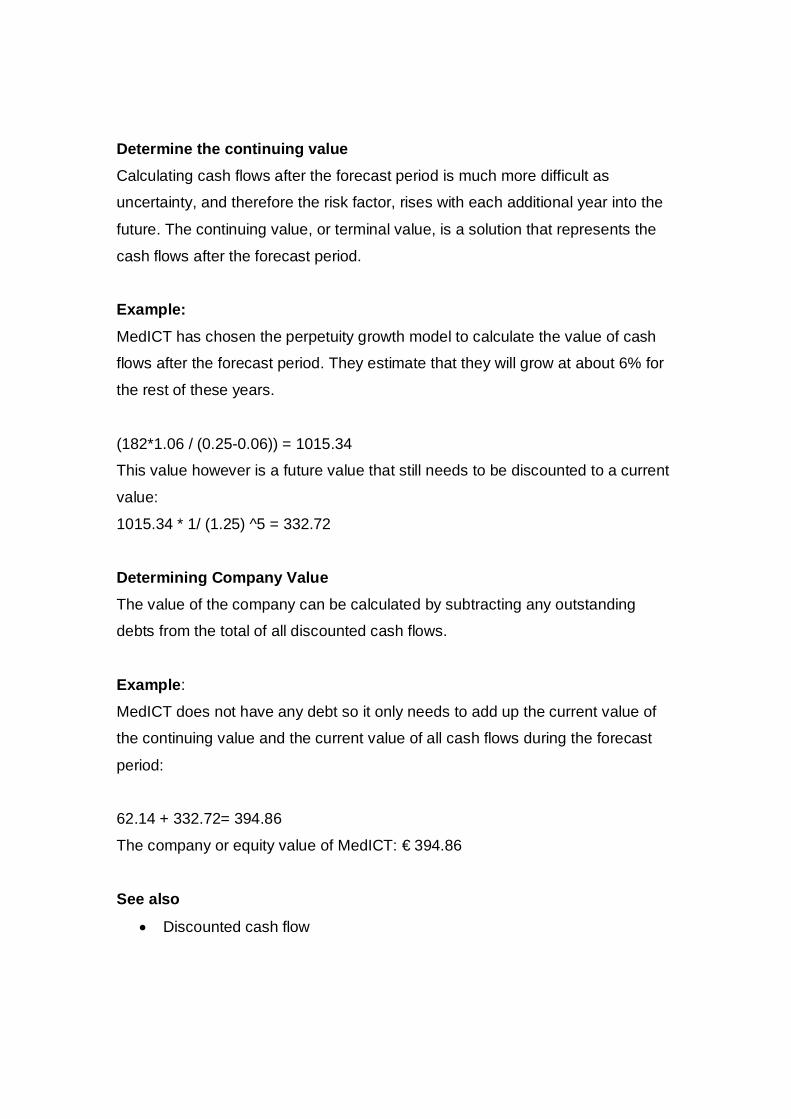
Determine the continuing value Calculating cash flows after the forecast period is much more difficult as
uncertainty, and therefore the risk factor, rises with each additional year into the
future. The continuing value, or terminal value, is a solution that represents the
cash flows after the forecast period.
Example:
MedICT has chosen the perpetuity growth model to calculate the value of cash
flows after the forecast period. They estimate that they will grow at about 6% for
the rest of these years.
(182*1.06 / (0.25-0.06)) = 1015.34
This value however is a future value that still needs to be discounted to a current
value:
1015.34 * 1/ (1.25) ^5 = 332.72
Determining Company Value The value of the company can be calculated by subtracting any outstanding
debts from the total of all discounted cash flows.
Example:
MedICT does not have any debt so it only needs to add up the current value of
the continuing value and the current value of all cash flows during the forecast
period:
62.14 + 332.72= 394.86
The company or equity value of MedICT: € 394.86
See also
Discounted cash flow

Literature
Kubr, Marchesi, Ilar, Kienhuis. 1998. Starting Up Mckinsey & Company
Pablo Fernandez. 2004. Equivalence of ten different discounted cash flow
valuation methods. IESE Research Papers D549
Ruback, R. S., 1995, an Introduction to Cash Flow Valuation Methods,
Harvard Business School Case # 295-155.
Keck, T., E. Levengood, and A. Longfield, 1998, Using Discounted Cash
Flow Analysis in an International Setting: A Survey of Issues in Modelling
the Cost of Capital, Journal of Applied Corporate Finance, fall, pp. 82-99.
Aswath Damodaran 2001 Investment Valuation: Tools and Techniques for
Determining Value Wiley
McKinsey & Co., Tim Koller, Marc Goedhart, David Wessels. 2005.
Valuation: Measuring and Managing the Value of Companies. John Wiley
& Sons
External links
Formulating the Imputed cost of equity capital
[http://www.newyorkfed.org/research/epr/03v09n3/0309gree.pdf], Federal
Reserve Bank of New York Includes a review of basic valuation models,
including DCF and CAPM
A Discounted Cash Flow Calculator
[http://www.moneychimp.com/articles/valuation/dcf.htm],
MoneyChimp.com
19) Real options analysis From Wikipedia, the free encyclopaedia
In corporate finance, real options analysis applies put option and call option
valuation techniques to capital budgeting decisions1.
A real option is the right but not the obligation, to undertake some business
decision, typically the option to make a capital investment. For example, the
opportunity to invest in the expansion of a firm's factory is a real option. In
contrast to financial options, a real option is not tradeable - e.g. the factory owner
cannot sell the right to extend his factory to another party, only he can make this
decision.
The terminology real option is relatively new, whereas business operators have
been making capital investment decisions for centuries. However, the description
of such opportunities as real options has occurred at the same time as thinking
about such decisions in new, more analytically based, ways. As such, the
terminology real option is closely tied to these new methods. The term real
option was coined by Professor Stewart Myers at the MIT Sloan School of
Management.
Certain critical components of real options make them a powerful analytical tool.
First, they recognize and value the flexibility that today's capital investments
provide. Second, they recognize the staged nature of many investments and
account explicitly for the reality that certain investments will never be made if --
based on additional information developed over time--they are deemed
unattractive. In these instances, it makes sense simply to abandon them, rather
than sink additional monies into a poor investment. By contrast, DCF (discounted
cash flow) evaluates a series of investments as if they will be made, regardless
of whether they still make sense later.
Additionally, with real option analysis, uncertainty inherent in investment projects
is usually accounted for by risk-adjusting probabilities (a technique known as the
equivalent martingale approach). Cash flows can then be discounted at the risk-
free rate. With regular DCF analysis, on the other hand, this uncertainty is
accounted for by adjusting the discount rate (using e.g. the cost of capital) or the
cash flows (using certainty equivalents). These methods normally do not properly

account for changes in risk over a project's lifecycle and fail to adapt
appropriately the risk adjustment. More importantly, the real options approach
forces decision makers to be more explicit about the assumptions underlying
their projections.
Another critical difference between DCF and real options is the effect of
uncertainty (or risk) on value. Uncertainty is typically considered bad for the
valuation of traditional cash flows. By contrast, uncertainty increases the value of
real options.
Real options are not universally recognized as a means of valuing capital
investments. Yet, the now ubiquitous capital asset pricing model did not become
a common pricing model overnight, either. Consider the following key points:
As volatility (uncertainty) increases, so does the value of the real option.
Initiatives with great uncertainty should be implemented in stages. Making a
small investment up front can give management the ability to resolve uncertainty
through data gathering and learning. The larger investment can be made in a
future environment with less uncertainty.
A series of initiatives should be looked at on a portfolio basis. The overall results
of the investment portfolio are what ultimately matters, not the individual
performance of each initiative. Real options recognize that abandonment is a
viable alternative that must be contemplated from the outset. Furthermore,
dropping a project does not necessarily mean that the team in charge of the
particular initiative has failed.
Technology investments might often grant the possibility of pursuing an avenue
in several months or a couple of years. However, without the relatively small
initial investment, an opportunity might be foreclosed forever.
Although real options can be intuitively appealing, execution to arrive at a value
is difficult. Determining the exact value of a real option is not necessarily critical.
Instead, understanding the drivers of the valuation and the value relative to
traditional methods is much more important.
This kind of option is not a derivative instrument, but an actual tangible option (in
the sense of choice) that a business may gain by undertaking certain
endeavours. For example, by investing in a project or property, a company may
have the real option of expanding, downsizing, or abandoning other projects in
the future. Other examples of real options may be opportunities for research and
development, mergers and acquisitions, licensing and film options.
These are called real options because they pertain to physical or tangible assets,
such as equipment, rather than financial instruments. Taking into account real
options can greatly affect the valuation of potential investments. However,
valuation methods, such as net present value (NPV), do not include the benefits
that real options might provide.
Generally, the most widely used methods are closed form solutions, partial
differential equations and the binomial lattices. In business strategy, real options
have been advanced by the construction of option space, where volatility is
compared with value-to-cost, NPVq.
References 1. Campbell, R. Harvey, ‘Identifying real options’
[http://faculty.fuqua.duke.edu/~charvey/Teaching/BA456_2002/Identifying_real_o
ptions.htm "Identifying real options”], Duke University, 2002
External links

Applications of option pricing theory to equity valuation
[http://pages.stern.nyu.edu/~adamodar/New_Home_Page/lectures/opt.ht
ml] Prof. Aswath Damodaran, Stern School of Business
How do you assess the value of a company's real options?
[http://www.expectationsinvesting.com/tutorial11.shtml], Prof. Alfred
Rappaport Columbia University and Michael Mauboussin
Real Options Tutorial [http://www.puc-rio.br/marco.ind/tutorial.html], Prof.
Marco Dias, Pontifícia Universidade Católica do Rio de Janeiro|PUC-Rio
Real Options Selected Links [http://sphere.rdc.puc-rio.br/marco.ind/ro-
links.html], Prof. Marco Dias, Pontifícia Universidade Católica do Rio de
Janeiro|PUC-Rio
An introduction to real options
[http://www.finance24.com/register/help/mmx_school/displayarticlewide.a
sp?ArticleID=328942] (PDF), The Investment Analysts Society of South
Africa
Applying Options Theories to Technology Management Decisions
[http://www.ctonet.org/documents/OptionsTheories_TechMgt.pdf], CTO
Network Library, 2005
Real Options Links and Resources at Money Science
[http://moneyscience.org/home/tiki-read_article.php?articleId=5]
Strategic Technology Investment Decisions in Research & Development
[http://lean.mit.edu/index.php?option=com_docman&task=doc_download
&gid=155] David Lackner MIT Lean Aerospace Initiative
20) Corporate finance From Wikipedia, the free encyclopaedia
Corporate finance is an area of finance dealing with the financial decisions
corporations make and the tools and analysis used to make these decisions. The
primary goal of corporate finance is to enhance corporate value while reducing
the firm's financial risks. Equivalently, the goal is to maximize the corporations'
return to capital. Although it is in principle different from managerial finance which
studies the financial decisions of all firms, rather than corporations alone, the
main concepts in the study of corporate finance are applicable to the financial
problems of all kinds of firms.
The discipline can be divided into long-term and short-term decisions and
techniques. Capital investment decisions are long-term choices about which
projects receive investment, whether to finance that investment with equity or
debt, and when or whether to pay dividends to shareholders. On the other hand,
the short-term decisions can be grouped under the heading working capital
management. This subject deals with the short-term balance of current assets
and current liabilities; the focus here is on managing cash, inventories, and short-
term borrowing and lending (such as the terms on credit extended to customers).
The terms corporate, finance and corporate financier are also associated with
investment banking. The typical role of an investment banker is to evaluate
investment projects for a bank to make investment decisions.
Capital investment decisions1 Capital investment decisions are long-term corporate finance decisions relating
to fixed assets and capital structure. Decisions are based on several inter-related
criteria. Corporate management seeks to maximize the value of the firm by
investing in projects, which yield a positive net present value when valued using
an appropriate discount rate. These projects must also be financed appropriately.
If no such opportunities exist, maximizing shareholder value dictates that
management return excess cash to shareholders. Capital investment decisions
thus comprise an investment decision, a financing decision, and a dividend
decision.

The investment decision Management must allocate limited resources between competing opportunities
(projects) in a process known as capital budgeting. Making this capital allocation
decision requires estimating the value of each opportunity or project: a function of
the size, timing and predictability of future cash flows.
Project valuation
In general, each project's value will be estimated using a discounted cash flow
(DCF) valuation, and the opportunity with the highest value, as measured by the
resultant net present value (NPV) will be selected (see Fisher separation
theorem). This requires estimating the size and timing of all of the incremental
cash flows resulting from the project. These future cash flows are then
discounted to determine their present value (see time value of money). These
present values are then summed, and this sum net of the initial investment outlay
is the net present value (NPV).
The net present value (NPV) is greatly influenced by the discount rate. Thus
selecting the proper discount rate - the project hurdle rate - is critical to making
the right decision. The hurdle rate is the minimum acceptable return on an
investment - i.e. the project appropriate discount rate. The hurdle rate should
reflect the riskiness of the investment, typically measured by volatility of cash
flows, and must take into account the financing mix.
Managers use models such as the capital asset pricing model (CAPM) or the
arbitrage pricing theory (APT) to estimate a discount rate appropriate for a
particular project, and use the weighted average cost of capital (WACC) to reflect
the financing mix selected. (A common error in choosing a discount rate for a
project is to apply a weighted average cost of capital (WACC) that applies to the
entire firm. Such an approach may not be appropriate where the risk of a
particular project differs markedly from that of the firm's existing portfolio of
assets.)

In conjunction with net present value (NPV), there are several other measures
used as (secondary) selection criteria in corporate finance. These are visible
from the discounted cash flow (DCF) and include payback, internal rate of return
(IRR), modified internal rate of return (MIRR), equivalent annuity, capital
efficiency, and return on investment (ROI).
See also: list of valuation topics, stock valuation, and fundamental analysis
Valuing flexibility In many cases, for example research and development (R&D) projects, a project
may open (or close) paths of action to the company, but this reality will not
typically be captured in a strict net present value (NPV) approach. Management
will therefore (sometimes) employ tools, which place an explicit value on these
options. Therefore, whereas in a discounted cash flow (DCF) valuation the most
likely, average, or scenario specific cash flows are discounted, here the flexible
and staged nature of the investment is modelled, and hence all potential payoffs
are considered. The difference between the two valuations is the option value
inherent in the project.
The two most common tools are decision tree analysis (DTA) and real option.
The decision tree analysis (DTA) approach attempts to capture flexibility
by incorporating likely events and consequent management decisions into
the valuation. In the decision tree, each management decision in response
to an event generates a branch or path, which the company could follow.
(For example, management will only proceed with stage 2 of the project
given that stage 1 was successful; stage 3, in turn, depends on stage 2. In
a discounted cash flow (DCF) model, on the other hand, there is no
branching - each scenario must be modelled separately.) The highest
value path (probability weighted) is regarded as representative of project
value

The real options approach is used when the value of a project is contingent on
the value of some other asset or underlying variable. (For example, the viability
of a mining project is contingent on the price of gold; if the price is too low,
management will abandon the mining rights, if sufficiently high, management will
develop the ore body. Again, a discounted cash flow (DCF) valuation would
capture only one of these outcomes.) Here, using financial option theory as a
framework, the decision to be taken is identified as corresponding to either a call
option or a put option - valuation is then via the binomial model or, less often for
this purpose, via Black Scholes; see Contingent claim valuation. The true value
of the project is then the net present value (NPV) of the most likely scenario plus
the option value.
The financing decision Achieving the goals of corporate finance requires that any corporate investment
be financed appropriately. As above, since both hurdle rate and cash flows (and
hence the riskiness of the firm) will be affected, the financing mix would have an
impact on the valuation. Management must therefore identify the optimal mix of
financing – the capital structure that results in maximum value. (See balance
sheet, weighted average cost of capital (WACC), Fisher separation theorem; but
see also the Modigliani-Miller theorem.)
The sources of financing will, generically, comprise some combination of debt
and equity. Financing a project through debt results in a liability that must be
serviced - and hence there are cash flow implications regardless of the project's
success. Equity financing is less risky in the sense of cash flow commitments,
but results in a dilution of ownership and earnings. The cost of equity is also
typically higher than the cost of debt (see Capital asset pricing model (CAPM)
and Weighted average cost of capital (WACC), and so equity financing may
result in an increased hurdle rate which may offset any reduction in cash flow
risk.

Management must also attempt to match the financing mix to the asset being
financed as closely as possible, in terms of both timing and cash flows. One of
the main theories of how firms make their financing decisions is the pecking
order theory, which suggests that firms avoid external financing while they have
internal financing available and avoid new equity financing while they can engage
in new debt financing at reasonably low interest rates.
Another major theory is the trade-off theory in which firms are assumed to trade-
off the tax benefits of debt with the bankruptcy costs of debt when making their
decisions. One last theory about this decision is the market-timing hypothesis,
which states that firms look for the cheaper type of financing regardless of their
current levels of internal resources, debt and equity.
The dividend decision In general, management must decide whether to invest in additional projects,
reinvest in existing operations, or return free cash as dividends to shareholders.
The dividend is calculated mainly based on the company's inappropriate profit
and its business prospects for the coming year. If there are no net present value
(NPV) positive opportunities, i.e. where returns exceed the hurdle rate, then
management must return excess cash to investors - these free cash flows
comprise cash remaining after all business expenses have been met. (This is
the general case however there are exceptions. For example, investors in a
growth stock, expect that the company almost by definition retain earnings to
fund growth internally. In other cases, even though an opportunity is currently
net present value (NPV) negative, management may consider investment
flexibility / potential payoffs and decide to retain cash flows; see above and real
options.)
Management must also decide on the form of the distribution, generally as cash
dividends or via a share buyback. There are various considerations: where
shareholders pay tax on dividends, companies may elect to retain earnings, or to

perform a stock buyback, in both cases increasing the value of shares
outstanding; some companies will pay dividends from stock rather than in cash.
(See corporate action) Today it is generally accepted that dividend policy is value
neutral (see Modigliani-Miller theorem).
Working capital management Decisions relating to working capital and short-term financing are referred to as
working capital management. These involve managing the relationship between
a firm's short-term assets and its short-term liabilities. The goal of working capital
management is to ensure that the firm is able to continue its operations and that
it has sufficient cash flow to satisfy both maturing short-term debt and upcoming
operational expenses.
Decision criteria By definition, Working capital management entails short-term decisions -
generally, relating to the next one-year period - which is reversible. These
decisions are therefore not taken on the same basis as capital investment
decisions (NPV or related, as above) rather they will be based on cash flows and
/ or profitability.
One measure of cash flow is provided by the cash conversion cycle - the
net number of days from the outlay of cash for raw material to receiving
payment from the customer. As a management tool, this metric makes
explicit the inter-relatedness of decisions relating to inventories, accounts
receivable and payable, and cash. Because this number effectively
corresponds to the time that the firm's cash is tied up in operations and
unavailable for other activities, management generally aims at a low net
count.
In this context, the most useful measure of profitability is return on capital
(ROC). The result is shown as a percentage, determined by dividing

relevant income for the 12 months by capital employed; return on equity
(ROE) shows this result for the firm's shareholders. Firm value is
enhanced when, and if, the return on capital, which results from working
capital management, exceeds the cost of capital, which results from
capital investment decisions as above. ROC measures are therefore
useful as a management tool, in that they link short-term policy with long-
term decision-making. See economic value added (EVA).
Management of working capital Guided by the above criteria, management will use a combination of policies and
techniques for the management of working capital. These policies aim at
managing the current assets (generally cash and cash equivalents, inventories
and debtors) and the short term financing, such that cash flows and returns are
acceptable.
Cash management: Identify the cash balance, which allows the business
to meet day-to-day expenses, but reduces cash holding costs.
Inventory management: Identify the level of inventory, which allows for
uninterrupted production but reduces the investment in raw materials - and
minimizes reordering costs - and hence increases cash flow (see supply
chain management; just in time (JIT), economic order quantity (EOQ),
economic production quantity (EPQ)).
Debtors management: Identify the appropriate credit policy, i.e. credit
terms which will attract customers, such that any impact on cash flows and
the cash conversion cycle will be offset by increased revenue and hence
return on capital (or vice versa); see discounts and allowances.
Short-term financing: Identify the appropriate source of financing, given
the cash conversion cycle: the inventory is ideally financed by credit

granted by the supplier; however, it may be necessary to utilize a bank
loan (or overdraft), or to convert debtors to cash through factoring.
Financial risk management
Risk management is the process of measuring risk and then developing and
implementing strategies to manage that risk. Financial risk management focuses
on risks that can be managed (hedged) using traded financial instruments
(typically, changes in commodity prices, interest rates, foreign exchange rates
and stock prices). Financial risk management will also play an important role in
cash management.
This area is related to corporate finance in two ways. Firstly, firm exposure to
business risk is a direct result of previous Investment and Financing decisions.
Secondly, both disciplines share the goal of creating, or enhancing, firm value.
All large corporations have risk management teams, and small firms practice
informal, if not formal, risk management.
Derivatives are the instruments most commonly used in financial risk
management. Because unique derivative contracts tend to be costly to create
and monitor, the most cost-effective financial risk management methods usually
involve derivatives that trade on well-established financial markets. These
standard derivative instruments include options, futures contracts, forward
contracts, and swaps.
:See: financial engineering; financial risk; default (finance); credit risk; interest
rate risk; liquidity risk; market risk; operational risk; volatility risk; settlement risk.
Relationship with other areas in finance Investment banking
Use of the term corporate finance varies considerably across the world. In the
United States, it is used, as above, to describe activities, decisions and
techniques that deal with many aspects of a company’s finances and capital. In
the United Kingdom and commonwealth countries, the terms corporate finance
and corporate financier tend to be associated with investment banking - i.e. with
transactions in which capital is raised for the corporation2.
Personal and public finance Corporate finance utilizes tools from almost all areas of finance. Some of the
tools developed by and for corporations have broad application to entities other
than corporations, for example, to partnerships, sole proprietorships, not-for-profit
organizations, governments, mutual funds, and personal wealth management.
However, in other cases their application is very limited outside of the corporate
finance arena. Because corporations deal in quantities of money much greater
than individuals do, the analysis has developed into a discipline of its own. It can
be differentiated from personal finance and public finance.
Related Professional Qualifications The new internationally recognised (http://www.cfqualification.com Corporate
Finance Qualification) (CF) is the only directly related professional qualification,
although many others traditionally can lead to the field:
Qualified accountant qualifications: Chartered Certified Accountant
(ACCA), Chartered Management Accountant (ACMA), Chartered
accountant (ACA), Certified Public Accountant (CPA)
Other non-statutory accountancy qualifications: Chartered Cost
Accountant (CCA Designation from AAFM), Certified Management
Accountant (CMA),
Business qualifications: Master of Business Administration (MBA), Master
of Finance & Control (MFC), Doctor of Business Administration (DBA)
Finance qualifications: Masters Degree in Finance (MSF), Corporate
Finance Qualification (http://www.cfqualification.com) (CF), Chartered
Financial Analyst (CFA), Certified International Investment Analyst (CIIA),

Association of Corporate Treasurers (ACT), Certified Market Analyst
(CMA/FAD) Dual Designation, and Master Financial Manager (MFM).
References 1The framework for this section is based on notes by Aswath Damodaran at New
York University's Stern School of Business
(http://pages.stern.nyu.edu/~adamodar/New_Home_Page/AppldCF/other/Image2
.gif)
2 Beaney, Shean, Defining corporate finance in the UK
(http://www.icaew.co.uk/index.cfm?route=122299), The Institute of Chartered
Accountants, April 2005.
See also
Business organizations
Financial planning
Investment bank and Investment Banking
Managerial economics
Private equity
Real option
Venture capital
Related topics by category:
List of accounting topics
List of corporate finance topics
List of valuation topics
List of finance topics alphabetical list

21) Modigliani-Miller theorem From Wikipedia, the free encyclopaedia
The Modigliani-Miller theorem (of Franco Modigliani, Merton Miller) forms the
basis for modern thinking on capital structure. The basic theorem states that, in
the absence of taxes, bankruptcy costs, and asymmetric information, and in an
efficient market, the value of a firm is unaffected by how that firm is financed1. It
does not matter if the firm's capital is raised by issuing stock or selling debt. It
does not matter what the firm's dividend policy is.
Propositions The theorem is made up of two propositions, which can also be extended to a
situation with taxes.
Consider two firms, which are identical except for their financial structures. The
first (Firm U) is unlevered: that is, it is financed by equity only. The other (Firm L)
is levered: it is financed partly by equity, and partly by debt. The Modigliani-Miller
theorem states that the value of the two firms is the same.
Without taxes Proposition I: VU = VL
Where VU is the value of an unlevered firm = price of buying a firm composed
only of equity, and VL is the value of a levered firm = price of buying a firm that is
composed of some mix of debt and equity.
To see why this should be true, suppose an investor is considering buying one of
the two firms U or L Instead of purchasing the shares of the levered firm L, he
could purchase the shares of firm U and borrow the same amount of money B
that firm L does. The eventual returns to either of these investments would be
the same. Therefore, the price of L must be the same as the price of U minus the
money borrowed B, which is the value of L's debt.

This discussion also clarifies the role of some of the theorem's assumptions. We
have implicitly assumed that the investor's cost of borrowing money is the same
as that of the firm, which need not be true in the presence of asymmetric
information or in the absence of efficient markets.
Proposition II: y =c0+ D/E (c0 - b)
y is the required rate of return on equity, or cost of equity.
c0 is the cost of capital for an all equity firm.
b is the required rate of return on borrowings, or cost of debt.
(D / E) is the debt-to-equity ratio.
This proposition states that the cost of equity is a linear function of the firm's debt
to equity ratio. A higher debt-to-equity ratio leads to a higher required return on
equity, because of the higher risk involved for equity-holders in a company with
debt. The formula is derived from the theory of weighted average cost of capital.
These propositions are true assuming the following assumptions:
no taxes exist,
no transaction costs exist, and
Individuals and corporations borrow at the same rates.
These results might seem irrelevant (after all, none of the conditions are met in
the real world), but the theorem is still taught and studied because it tells us
something very important. That is, if capital structure matters, it is precisely
because one or more of the assumptions is violated. It tells us where to look for
determinants of optimal capital structure and how those factors might affect
optimal capital structure.

With taxes Proposition 1:
VL =VU + TC D
where
VL is the value of a levered firm.
VU is the value of an unlevered firm.
TC D is the tax rate (TC) x the value of debt (D)
This means that there are advantages for firms to be levered, since corporations
can deduct interest payments. Therefore, leverage lowers tax payments.
Dividend payments are non-deductible.
Proposition II:
y = c0 + D / E (c0 - b) (1-TC)
where
y is the required rate of return on equity, or cost of equity.
c0 is the cost of capital for an all equity firm.
b is the required rate of return on borrowings, or cost of debt.
(D / E) is the debt-to-equity ratio.
Tc is the tax rate.
The same relationship as earlier described stating that the cost of equity rises
with leverage, because the risk to equity rises, still holds. The formula however
has implications for the difference with the WACC.
The following assumptions are made in the propositions with taxes:
corporations are taxed at the rate TC on earnings after interest,
no transaction cost exist, and
individuals and corporations borrow at the same rate
Miller and Modigliani published a number of follow-up papers discussing some of
these issues.

The theorem first appeared in F. Modigliani and M. Miller, "The Cost of Capital,
Corporation Finance and the Theory of Investment," American Economic Review
(http://www.aeaweb.org/aer/) (June 1958).
See also
Weighted average cost of capital
Debt to equity ratio
Arbitrage pricing theory
Cost of capital
John Burr Williams
Footnotes 1 MIT Sloan Lecture Notes, Finance Theory II, Dirk Jenter, 2003
References
Brealy and Myers, Principles of Corporate Finance
G. Bennett Stewart III, 'The Quest for Value' (HarperCollins, 1991)
F. Modigliani and M. Miller, ‘The Cost of Capital, Corporation Finance and
the Theory of Investment,’ American Economic Review (June 1958).
M. Miller and F. Modigliani: ‘Corporate income taxes and the cost of
capital: a correction.’ American Economic Review, 53 (3) (1963), pp. 433-
443.
J. Miles und J. Ezzell: ‘The weighted average cost of capital, perfect
capital markets and project life: a clarification.’ Journal of Financial and
Quantitative Analysis, 15 (1980), S. 719-730.
Links
MIT Sloan Lecture Notes, Finance Theory II, Dirk Jenter, 2003
(http://ocw.mit.edu/NR/rdonlyres/Sloan-School-of-Management/15-
402Finance-Theory-IISpring2003/96178A76-03FF-426A-8AE6
5A6F014F8BF1/0/lec10awrapupfinancing.pdf)
Corporate Finance: The Modigliani-Miller Theorems
(http://courses.essex.ac.uk/EC/EC372/ec372mm.pdf)
Ruben D Cohen ‘An Implication of the Modigliani-Miller Capital Structuring
Theorems on the Relation between Equity and Debt’
(http://rdcohen.50megs.com/MMabstract.htm download)
22) Cost of capital From Wikipedia, the free encyclopaedia
The cost of capital for a firm is a weighted sum of the cost of equity and the cost
of debt (see the financing decision). Firms finance their operations by three
mechanisms: issuing stock (equity), issuing debt (borrowing from a bank is
equivalent for this purpose) (those two are external financing), and reinvesting
prior earnings (internal financing).
Summary Capital (money) used to fund a business should earn returns for the capital
owner who risked their saved money. For an investment to be worthwhile, the
estimated return on capital must be greater than the cost of capital. Otherwise
stated, the risk-adjusted return on capital (incorporating not just the projected
returns, but also the probabilities of those projections) must be higher than the
cost of capital.
The cost of debt is relatively simple to calculate, as it is composed of the interest
paid (interest rate), including the cost of risk (the risk of default on the debt). In
practice, the interest paid by the company will include the risk-free rate and a risk
component, which itself incorporates a probable rate of default (and amount of
recovery given default). For companies with similar risk or credit ratings, the
interest rate is largely exogenous.
Cost of equity is more challenging to calculate, as equity does not pay a set
return to its investors. Similar to the cost of debt, the cost of equity is broadly

defined as the risk-weighted projected return required by investors, where the
return is largely unknown. The cost of equity is therefore inferred by comparing
the investment to other investments with similar risk profiles to determine the
market cost of equity.
The cost of capital is often used as the discount rate, the rate at which projected
cash flow will be discounted to give a present value or net present value.
Cost of debt The cost of debt is computed by taking the rate on a non-defaulting bond whose
duration matches the term structure of the corporate debt, then adding a default
premium. This default premium will rise as the amount of debt increases (since
the risk rises as the amount of debt rises). Since in most cases debt expenses is
a deductible expense, the cost of debt is computed as an after tax cost to make it
comparable with the cost of equity (earnings are after-tax as well). Thus, for
profitable firms, debt is discounted by the tax rate. This is used for large
corporations only.
Cost of equity
Expected return The expected return can be calculated as the dividend capitalization model,
which are (dividend per share / price per share) + growth rate of dividends.
Which is the dividend yield + growth rate of dividends*dividend.
Capital asset pricing model The capital asset pricing model (CAPM) is used in finance to determine a
theoretically appropriate price of an asset such as a security. The expected
return on equity according to the capital asset pricing model, the market risk is
normally characterized by the β parameter and thus the investors would expect
(or demand) to receive:

Es = Rf + βs (Rm - Rf)
Where:
Es The expected return for a security
Rf The expected risk-free return in that market (government bond yield)
βs The sensitivity to market risk for the security
RM The historical return of the equity market
(RM-Rf) The risk premium of market assets over risk free assets
In writing:
The expected return (%) = risk-free return (%) + sensitivity to market risk *
(historical return (%) - risk-free return (%))
Put another way the expected rate of return (%) = the yield on the treasury
note closest to the term of your project + the beta of your project or
security * (the market risk premium)
the market risk premium has historically been between 3-5%
Comments The models state that investors will expect a return that is the risk-free return
plus the security's sensitivity to market risk times the market risk premium.
The risk free rate is taken from the lowest yielding bonds in the particular market,
such as government bonds.
The risk premium varies over time and place, but in some developed countries
during the twentieth century, it has averaged around 5%. The equity market real
capital gain return has been about the same as annual real GDP growth. The
capital gains on the Dow Industrials have been 1.6% per year over the period
1910-2005 (http://home.earthlink.net/~intelligentbear/com-dj-infl.htm). The
dividends have increased the total real return on average equity to the double,
about 3.2%.

The sensitivity to market risk (β) is unique for each firm and depends on
everything from management to its business and capital structure. This value
cannot be known ex ante (beforehand), but can be estimated from ex post (past)
returns and experience with similar firms.
Note that retained earnings are a component of equity, and therefore the cost of
retained earnings is equal to the cost of equity. Dividends (earnings that are paid
to investors and not retained) are a component of the return on capital to equity
holders, and influence the cost of capital through that mechanism.
Weighted average cost of capital
The Weighted Average Cost of Capital (WACC) is used in finance to measure a
firm's cost of capital. The total capital for a firm is the value of its equity (for a firm
without outstanding warrants and options, this is the same as the company's
market capitalization) plus the cost of its debt (the cost of debt should be
continually updated as the cost of debt changes because of interest rate
changes). Notice that the equity in the debt to equity ratio is the market value of
all equity, not the shareholders' equity on the balance sheet.
Formula
The cost of capital is then given as:
Kc = (1-δ)Ke + δKd
Where:
Kc The weighted cost of capital for the firm
δ The debt to capital ratio, D / (D + E)
Ke The cost of equity
Kd The after tax cost of debt
D The market value of the firm's debt, including bank loans and leases
E The market value of all equity (including warrants, options, and the equity
portion of convertible securities)
In writing:

WACC = (1 - debt to capital ratio) * cost of equity + debt to capital ratio * cost of
debt
Capital structure Because of tax advantages on debt issuance, it will be cheaper to issue debt
rather than new equity (this is only true for profitable firms, tax breaks are
available only to profitable firms). At some point, however, the cost of issuing
new debt will be greater than the cost of issuing new equity. This is because
adding debt increases the default risk - and thus the interest rate that the
company must pay in order to borrow money. By utilizing too much debt in its
capital structure, this increased default risk can also drive up the costs for other
sources (such as retained earnings and preferred stock) as well. Management
must identify the optimal mix of financing – the capital structure where the cost of
capital is minimized so that the firm’s value can be maximized.
The Thomson financial league tables show that global debt issuance exceeds
equity issuance with a 90 to 10 margin.
Modigliani-Miller theorem
If there were no tax advantages for issuing debt, and equity could be freely
issued, Miller and Modigliani showed that the value of a leveraged firm and the
value of an unleveraged firm should be the same. (Their paper is foundational in
modern corporate finance.)
References
F. Modigliani and M. Miller, ‘The Cost of Capital, Corporation Finance and
the Theory of Investment,’ American Economic Review (June 1958).
See also
Capital asset pricing model
Modigliani-Miller theorem

Weighted average cost of capital
Net present value
External links Definition
Cost of Equity (http://www.investopedia.com/terms/c/costofequity.asp)
Articles
Dividend Irrelevancy and Price-Earning Ratios
(http://papers.ssrn.com/sol3/papers.cfm?abstract_id=667781)
TeachMeFinance.com - Cost of Capital
([http://teachmefinance.com/costofcapital.html)
23) Leveraged buyout From Wikipedia, the free encyclopaedia
A leveraged buyout (or LBO, or highly leveraged transaction (HLT), or bootstrap
transaction) occurs when a financial sponsor gains control of a majority of a
target company's equity with borrowed money or debt.
A leveraged buyout is a strategy involving the acquisition of another company
using a significant amount of borrowed money (bonds or loans) to meet the cost
of acquisition. Often, the assets of the company being acquired are used as
collateral for the loans, in addition to the assets of the acquiring company. The
purpose of leveraged buyouts is to allow companies to make large acquisitions
without having to commit a lot of capital. In a LBO, there is usually a ratio of 70%
debt to 30% equity, although debt can reach as high as 90% to 95% of the target
company's total capitalization. The equity component of the purchase price is
typically provided by a pool of private equity capital.

Typically, the loan capital is borrowed through a combination of prepay able bank
facilities and/or public or privately placed bonds, which may be classified as high-
yield debt, also called junk bonds. Often, the debt will appear on the acquired
company's balance sheet and the acquired company's free cash flow will be used
to repay the debt.
History
In the industry's infancy in the late 1960s, the acquisitions were called "bootstrap"
transactions, and were characterized by Victor Posner's hostile takeover of
Sharon Steel Corporation in 1969. The industry was conceived by people like
Jerome Kohlberg, Jr. while working on Wall Street in the 1960s and 1970s, and
pioneered by the firm he helped found with Henry Kravis, Kohlberg Kravis
Roberts & Co. (KKR).
KKR is credited by Harvard Business School as completing what is believed to
be the first leveraged buyout in business history, through the acquisition of Orkin
Exterminating Company in 1964. However, the first LBO may have been the
purchase by McLean Industries, Inc. of Waterman Steamship Corporation in May
1955. Under the terms of that transaction, McLean borrowed $42 million and
raised an additional $7 million through issue of preferred stock. When the deal
closed, $20 million of Waterman cash and assets were used to retire $20 million
of the loan debt. The newly elected board of Waterman then voted to pay an
immediate dividend of $25 million to McLean Industries1.
Rationale The purposes of debt financing for leveraged buyouts are two-fold:
The use of debt increases (leverages) the financial return to the private equity
sponsor. Under the Modigliani-Miller theorem2 the total return of an asset to its
owners, all else being equal and within strict restrictive assumptions, is
unaffected by the structure of its financing. As the debt in a LBO has a relatively

fixed, albeit high cost of capital, any returns in excess of this cost of capital flow
through to the equity.
The tax shield of the acquisition debt, according to the Modigliani-Miller theorem
with taxes, increases the value of the firm. This enables the private equity
sponsor to pay a higher price than would otherwise be possible. Because income
flowing through to equity is taxed, while interest payments to debt are not, the
capitalized value of cash flowing to debt is greater than the same cash stream
flowing to equity.
Historically, many LBOs in the 1980s and 1990s focused on reducing wasteful
expenditures by corporate managers whose interests were not aligned with
shareholders. After a major corporate restructuring, which may involve selling off
portions of the company and severe staff reductions, the entity would likely be
producing a higher income stream. Because this type of management arbitrage
and easy restructuring has largely been accomplished, LBOs today (2007) focus
more on growth and complicated financial engineering to achieve their returns
Most leveraged buyout firms look to achieve an internal rate of return in excess
of 20%.
Management buyouts A special case of such acquisition is a management buyout (MBO), which
occurs when a company's managers buy or acquire a large part of the company.
The goal of an MBO may be to strengthen the managers' interest in the success
of the company. In most cases, the management will then take the company
private. MBOs have assumed an important role in corporate restructurings
beside mergers and acquisitions. Key considerations in an MBO are fairness to
shareholders, price, the future business plan, and legal and tax issues.

Failures Some leveraged buyouts (LBO) in the 1980s and 1990s resulted in corporate
bankruptcy, such as Robert Campeau's 1988 buyout of Federated Department
Stores and the 1986 buyout of the Revco drug stores. The failure of the
Federated buyout was a result of excessive debt financing, comprising about
97% of the total consideration, which led to large interest payments that
exceeded the company's operating cash flow. In response to the threat of
leveraged buyouts (LBO), certain companies had adopted a number of
techniques, such as the poison pill to protect them against hostile takeovers by
effectively self-destruct the company if it were to be taken over.
Notable leveraged buyout firms
Apollo
Bain Capital
The Blackstone Group
The Carlyle Group
Goldman Sachs Capital Partners
Kohlberg Kravis Roberts & Co.
Providence Equity Partners
TA Associates
Texas Pacific Group
Warburg Pincus
Europe-based
3i
Apax Partners
AXA Private Equity
Barclays Private Equity
BC Partners
Candover
Cinven

CVC Capital Partners
PAI Partners
Permira
Palaka Bazaar
Terra Firma Capital Partners
See also
Private equity
Bootstrap
Divisional Buyout
Notes 1 Marc Levinson, The Box, How the Shipping Container Made the World
Smaller and the World Economy Bigger, pp. 44-47 (Princeton Univ. Press
2006) The details of this transaction are set out in ICC Case No. MC-F-
5976, McLean Trucking Company and Pan-Atlantic American Steamship
Corporation--Investigation of Control, July 8, 1957.
2 Franco Modigliani and Merton H. Miller, The Cost of Capital, Corporation
Finance, and the Theory of Investment, American Economic Review'',
June 1958.
External links
Financial dictionary: Bootstrap transaction
(http://www.specialinvestor.com/terms/93.html)
Buyout Blog (http://www.pehub.com) Industry commentary
Feb 1993 - The CPA Journal Online
(http://www.nysscpa.org/cpajournal/old/13808663.htm) (accounting for a
bootstrap transaction)
Challenges Faced In Executing Leveraged Buyouts in India - The
Evolution of the Growth Buyout

(http://w4.stern.nyu.edu/glucksman/docs/Chokshi.pdf) by Narendra
Chokshi (http://www.geocities.com/narendra.chokshi), NYU Stern
Category: private equity
24) Capital structure From Wikipedia, the free encyclopaedia
Capital structure refers to the way a corporation finances itself through some
combination of equity sales, equity options, bonds, and loans. A firm's capital
structure is then the composition or structure of its liabilities. For example, a firm
that sells $20bn dollars in equity and $80bn in debt is said to be 20% equity
financed and 80% debt financed. The firm's ratio of debt to total financing, 80% in
this example is referred to as the firm's leverage.
The Modigliani-Miller theorem, proposed by Franco Modigliani and Merton Miller
forms the basis for modern thinking on capital structure, though it is generally
viewed as a purely theoretical result since it assumes away many important
factors in the capital structure decision. The theorem states that, in the absence
of tax effect, bankruptcy cost, transaction cost, and asymmetric information, and
if the equity market is efficient, the value of a firm is unaffected by the way in
which that firm is financed.
Optimal capital structure A firm's optimal capital structure refers to the particular combination of liabilities
(debt, equity or any other) that maximizes the value of the firm. An optimal
capital structure, if one exists, would allow a corporation to maximize the value of

the firm. The identity of the factors that affect this optimum is an important for
financial economics.
For example, the manager's incentives to work hard increase change if the firm is
highly indebted, since his or her job is in peril. If that is true, then the firm is more
valuable as a whole by having a lot of debt in its capital structure. These types of
considerations motivate the study of an optimal combination of liabilities that
would maximize the alignment of incentives, and minimize taxes, bankruptcy
costs etc.
Attention is usually given to the tax effect of debt, risk or bankruptcy risk, as
excessive leverage can endanger a business's through insolvency, the
informational advantages that managers have over investors - in short all the
factors left out of the Modigliani-Miller theorem. These factors can adversely
affect the stock price by increasing risk premium.
Alternative Capital Structure Theories
The Static Trade-Off Theory - optimal capital structure represents a trade-
off between tax benefits of debt and bankruptcy costs
The managerial incentives theory (also known as the agency theory) -
optimal capital structure describes the optimal control mechanism for
adverse incentives created by too little debt and adverse incentives
created by too much debt
The Pecking Order Theory - optimal capital structure at any time depends
on minimum mispricing due to outsiders being less informed than insiders
The neutral mutation hypothesis - firms fall into various habits of financing
which do not impact on value
Market timing hypothesis - capital structure is the outcome of the historical
cumulative timing of the market by managers (Baker and Wurlger).

Arbitrage Similar questions are also the concern of a variety of speculator known as a
capital-structure arbitrageur. See arbitrage.
A capital-structure arbitrageur seeks opportunities created by differential pricing
of various instruments issued by one corporation. Consider, for example,
traditional bonds and convertible bonds. The latter are bonds that are, under
contracted-for conditions, convertible into shares of equity. The stock-option
component of a convertible bond has a calculable value in itself. The value of the
whole instrument should be the value of the traditional bonds plus the extra value
of the option feature. If the spread, the difference between the convertible and
the non-convertible bonds grows excessively, then the capital-structure
arbitrageur will bet that it will converge.
See also
Capital structure theory
Financial economics
Debt to equity ratio
Leverage (finance)
Modigliani-Miller theorem
market timing hypothesis
Ruben D Cohen Articles
Ruben D Cohen (2004) ‘An Analytical Process for Generating the WACC
Curve and Locating the Optimal Capital Structure (download
http://rdcohen.50megs.com/OCSabstract.htm),’ Wilmott Magazine,
November issue
Ruben D Cohen (2005) ‘Working Excel Spreadsheet’ [download
(http://rdcohen.50megs.com/OCSspreadsheet.htm)]

Ruben D Cohen (2004) ‘The Optimal Capital Structure of Depository
Institutions [download (http://rdcohen.50megs.com/DepInstabstract.htm)],
Wilmott Magazine, March issue.
Ruben D Cohen (2005) ‘A Generalised Procedure for Locating the Optimal
Capital Structure [download
(http://rdcohen.50megs.com/genOCSabstract.htm],’ Wilmott Magazine,
November issue
Ruben D Cohen (2007) Incorporating default risk into Hamada's equation
for application to capital structure [download
(http://rdcohen.50megs.com/IDRHEqabstract.htm)],
External Links
http://www.investopedia.com/terms/c/capitalstructure.asp
http://www.westga.edu/~bquest/2002/rethinking.htm
25) Takeover From Wikipedia, the free encyclopaedia
A takeover in business refers to one company (the acquirer, or bidder)
purchasing another (the target). In the UK, the term properly refers to the
acquisition of a public company whose shares are listed on a stock exchange, in
contrast to the acquisition of a private company.
Friendly and hostile takeovers When a bidder makes an offer for another company, it will usually inform the
board of the target beforehand. If the board feels that the offer is such that the
shareholders will be best served by accepting, it will recommend the offer be
accepted by the shareholders. A takeover would be considered hostile if (1) the
board rejects the offer, but the bidder continues to pursue it or (2 if the bidder
makes the offer without informing the board beforehand.
The main consequence of a bid being considered hostile is practical rather than
legal. If the board of the target cooperates, the bidder will be able to conduct
extensive due diligence into the affairs of the target company. It will be able to
find out exactly what it is taking on before it makes a commitment. A hostile
bidder will know only the information on the company that is publicly available
and will therefore be taking more of a risk. Banks are also less willing to back
hostile bids with the loans that are usually needed to finance the takeover.
In a private company, the shareholders and the board either are likely to be the
same people or closely connected with one another. Therefore, all private
acquisitions are likely to be friendly, because if the shareholders have agreed to
sell the company then the board, however comprised, will usually be of the same
mind or be sufficiently under the orders of the shareholders to cooperate with the
bidder. This point is not relevant to the UK concept of takeovers, which always
involve the acquisition of a public company.
In cases where management may not be acting in the best interest of the
shareholders (or creditors, in cases of bankrupt firms), a hostile takeover allows a
suitor to bypass intransigent management. In this case, this enables the
shareholders to choose the option that may be best for them, rather than leaving
approval solely with management. In this case, a hostile takeover may be
beneficial to shareholders, which is contrary to the usual perception that a hostile
takeover is bad.
Reverse takeovers
A reverse takeover is a type of takeover where a public company acquires a
private company of a higher value. This is usually done at the instigation of the
larger, private company, the purpose being for the private company to float

effectively itself while avoiding some of the expense and time involved in a
conventional initial public offering (IPO).
Financing a takeover Cash A company acquiring another will frequently pay for the other company by cash.
The cash can be raised in a number of ways. The company may have sufficient
cash available in its account, but this is unlikely. More often, the cash will be
borrowed from a bank, or raised by an issue of bonds. Acquisitions financed
through debt are known as leveraged buyouts, and the debt will often be moved
down onto the balance sheet of the acquired company. The acquired company
then has to pay back the debt. This is a technique often used by private equity
companies. The debt ratio of financing can go as high as 80% in some cases.
Then to acquire a company, you actually need to finance only 30% of the
purchasing price.
Loan note alternatives Cash offers for public companies frequently include a loan note alternative that
allows shareholders to take part or all of their consideration in loan notes rather
than cash. This is done primarily to make the offer more attractive in terms of
taxation - a conversion of shares into cash is counted a disposal that will trigger a
payment of capital gains tax, whereas if the shares are converted into other
securities, such as loan notes, the tax is rolled over.
All share deals A takeover, particularly a reverse takeover, may be financed by an all share deal.
The bidder does not pay money, but instead issues new shares in it to the
shareholders of the company being acquired. In a reverse takeover, the
shareholders of the company being acquired will end up with a majority of the
shares in, and therefore control of, the company making the bid.

Takeover mechanics Takeovers in the United Kingdom
Takeovers in the UK (meaning acquisitions of public companies only) are
governed by the city code on takeovers and mergers, also known as the city
code or takeover code. The rules for a takeover can be found what is primarily
known as 'The Blue Book'. The code used to be a non-statutory set of rules that
was controlled by city institutions on a theoretically voluntary basis. However, as
a breach of the Code brought such reputational damage and the possibility of
exclusion from city services run by those institutions, it was regarded as binding.
In 2006, the code was put onto a statutory footing as part of the UK's compliance
with the European Directive on Takeovers (http://europa.eu/eur-
lex/pri/en/oj/dat/2004/l_142/l_14220040430en00120023.pdf) (2004/25/EC).
The code requires that all shareholders in a company should be treated equally,
regulates when and what information companies must and cannot release
publicly in relation to the bid, sets timetables for certain aspects of the bid, and
sets minimum bid levels following a previous purchase of shares.
In particular:
a shareholder must make an offer when its shareholding, including that of
parties acting in concert (a concert party), reaches 30% of the target;
information relating to the bid must not be released except by
announcements regulated by the code;
the bidder must make an announcement if rumour or speculation have
affected a company's share price;
the level of the offer must not be less than any price paid by the bidder in
the three months before the announcement of a firm intention to make an
offer;
if shares are bought during the offer period at a price higher than the offer
price, the offer must be increased to that price;
The rules governing the substantial acquisition of shares, which used to
accompany the code and which regulated the announcement of certain levels of
shareholdings, have now been abolished, though similar provisions still exist in
the company’s act 1985.
Strategies There are varieties of reasons why an acquiring company may wish to purchase
another company. Some takeovers are opportunistic - the target company may
simply be very reasonably priced for one reason or another and the acquiring
company may decide that in the long run, it will end up making money by
purchasing the target company. The large holding company Berkshire Hathaway
has profited well over time by purchasing many companies opportunistically in
this manner.
Other takeovers are strategic in that they are thought to have secondary effects
beyond the simple effect of the profitability of the target company being added to
the acquiring company's profitability. For example, an acquiring company may
decide to purchase a company that is profitable and has good distribution
capabilities in new areas, which the acquiring company can utilize for its own
products as well.
A target company might be attractive because it allows the acquiring company to
enter a new market without having to take on the risk, time and expense of
starting a new division. An acquiring company could decide to take over a
competitor not only because the competitor is profitable, but in order to eliminate
competition in its field and make it easier, in the long term, to raise prices. In
addition, a takeover could fulfil the belief that the combined company can be
more profitable than the two companies would be separately due to a reduction
of redundant functions.

Critics often charge that large companies initiate takeovers in order to boost their
reported revenue (sales to customers) without giving sufficient regard to profit,
which generally takes a hit when a company is acquired because of all the
associated costs. In addition, a premium is always paid if the target company is
financially healthy and not already desperate to be taken over.
The target company has several methods to avoid a takeover, if it wishes. These
include legal actions, as in the case of the Hewlett-Packard purchase of Compaq,
or the use of a poison pill, as set up by Transmeta.
Most dot-com companies were created for the express purpose of being taken
over with a consequent immediate profit for their owners, as opposed to the
usual purpose of creating a business: to create profit for its owners over time by
generating cash which is paid in dividends.
Perceived pros and cons of takeover Perceived pros and cons of a takeover differ from case to case but still there are
a few worth mentioning.
Pros:
1 Increase in sales/revenues (e.g. Procter & Gamble takeover of Gillette)
2 Venture into new businesses and markets
3 Profitability of target company
4 Increase market share
5 Decrease competition (from the perspective of the acquiring company)
6 Reduction of overcapacity in the industry
7 Enlarge brand portfolio (e.g. L'Oréal's takeover of Body shop)
Cons:
1 Reduced competition and choice for consumers in oligopoly markets
2 Likelihood of price increases and job cuts
3 Cultural integration/conflict with new management
4 Hidden liabilities of target entity

Occurrence Corporate takeovers occur readily in the United States, the United Kingdom and
France. They happen only occasionally in Italy because larger shareholders
(typically controlling families) often have special board voting privileges designed
to keep them in control. They do not happen often in Germany because of the
dual board structure or in Japan because companies have interlocking sets of
ownerships known as keiretsu, nor in the People's Republic of China because
the state majority-owns most publicly listed companies.
26) Mergers and Acquisitions From Wikipedia, the free encyclopaedia
The phrase mergers and acquisitions (abbreviated M&A) refers to the aspect of
corporate strategy, corporate finance and management dealing with the buying,
selling and combining of different companies.
Overview Merger is a tool used by companies for expanding their operations often aiming
at an increase of their long-term profitability. Evidence on the success of M&A
however is mixed: 50-75% of all M&A deals are found to fail in their aim of adding
value.
Usually mergers occur in a consensual (occurring by mutual consent) setting
where executives from the target company help those from the purchaser in a
due diligence process to ensure that the deal is beneficial to both parties.
Acquisitions can also happen through a hostile takeover by purchasing the
majority of outstanding shares of a company in the open market against the
wishes of the target's board. In the United States, business laws vary from state
to state whereby some companies have limited protection against hostile

takeovers. One form of protection against a hostile takeover is the shareholder
rights plan, otherwise known as the poison pill.
Historically, mergers have often failed to add significantly to the value of the
acquiring firm's shares (King, et al., 2004). Corporate mergers may be aimed at
reducing market competition, cutting costs (for example, laying off employees,
operating at a more technologically efficient scale, etc.), reducing taxes,
removing management, empire building by the acquiring managers, or other
purposes which may or may not be consistent with public policy or public welfare.
Thus, they can be heavily regulated, for example, in the U.S. requiring approval
by both the Federal Trade Commission and the Department of Justice.
The U.S. began their regulation on mergers in 1890 with the implementation of
the Sherman Act. It was meant to prevent any attempt to monopolize or to
conspire to restrict trade. However, based on the loose interpretation of the
standard ‘Rule of Reason’, it was up to the judges in the U.S. supreme court
whether to rule leniently (as with U.S. Steel in 1920) or strictly (as with Alcoa in
1945).
Acquisition An acquisition, also known as a takeover, is the buying of one company (the
target) by another. An acquisition may be friendly or hostile. In the former case,
the companies cooperate in negotiations; in the latter case, the takeover target is
unwilling to be bought or the target's board has no prior knowledge of the offer.
Acquisition usually refers to a purchase of a smaller firm by a larger one.
Sometimes, however, a smaller firm will acquire management control of a larger
or longer established company and keep its name for the combined entity. This is
known as a reverse takeover.
Types of acquisition
The buyer buys the shares, and therefore control, of the target company.
The buyer buys the assets of the target. This type of transaction leaves
the target company as an empty shell, if the buyer buys out the entire
assets. The cash the target receives from the sell-off is paid back to its
shareholders by dividend or through liquidation. A buyer executes asset
purchase, often to cherry-pick the assets that it wants and leave out the
assets and liabilities that it does not.
The terms demerger, spin-off and spinout are sometimes used to indicate a
situation where one company splits into two, generating a second company
separately listed on a stock exchange.
Merger In business or economics, a merger is a combination of two companies into one
larger company. Such actions are commonly voluntary and involve stock swap or
cash payment to the target. Stock swap is often used as it allows the
shareholders of the two companies to share the risk involved in the deal. A
merger can resemble a takeover but result in a new company name (often
combining the names of the original companies) and in new branding; in some
cases, terming the combination a merger rather than an acquisition is done
purely for political or marketing reasons.
Classifications of mergers
Horizontal mergers take place where the two merging companies produce
similar product in the same industry.
Vertical mergers occur when two firms, each working at different stages in
the production of the same good, combine.
Conglomerate mergers take place when the two firms operate in different
industries.
A unique type of merger called a reverse merger is used as a way of going public
without the expense and time required by an IPO.
The contract vehicle for achieving a merger is a merger sub.
The occurrence of a merger often raises concerns in antitrust circles. Devices
such as the Herfindahl index can analyze the impact of a merger on a market
and what, if any, action could prevent it. Regulatory bodies such as the European
Commission and the United States Department of Justice may investigate anti-
trust cases for monopolies dangers, and have the power to block mergers.
Accretive mergers are those in which an acquiring company's earnings per share
(EPS) increase. An alternative way of calculating this is if a company with a high
price to earnings ratio (P/E) acquires one with a low price to earnings ratio (P/E).
Dilutive mergers are the opposite of above, whereby a company's earnings per
share (EPS) decrease. The company will be one with a low price to earnings
ratio (P/E), acquiring one with a high price to earnings ratio (P/E).
The completion of a merger does not ensure the success of the resulting
organization; indeed, many mergers (in some industries, the majority) result in a
net loss of value due to problems. Correcting problems caused by incompatibility
-whether of technology, equipment, or corporate culture - diverts resources away
from new investment, and these problems may be exacerbated by inadequate
research or by concealment of losses or liabilities by one of the partners.
Overlapping subsidiaries or redundant staff may be allowed to continue, creating
inefficiency, and conversely the new management may cut too many operations
or personnel, losing expertise and disrupting employee culture. These problems
are similar to those encountered in takeovers. For the merger not to be
considered a failure, it must increase shareholder value faster than if the
companies were separate, or prevent the deterioration of shareholder value more
than if the companies were separate.

Financing M&A Mergers are generally differentiated from acquisitions partly by the way in which
they are financed and partly by the relative size of the companies. Various
methods of financing an M&A deal exist:
Cash Payment by cash such transactions are usually termed acquisitions rather than
mergers because the shareholders of the target company are removed from the
picture and the target comes under the (indirect) control of the bidder's
shareholders alone.
Financing Financing cash can be borrowed from a bank, or raised by an issue of bonds.
Acquisitions financed through debt are known as leveraged buyouts, and the
debt will often be moved down onto the balance sheet of the acquired company.
A cash deal would make more sense during a downward trend in the interest
rates. Another advantage of using cash for an acquisition is that there tends to
lesser chances of EPS dilution for the acquiring company. However, a caveat in
using cash is that it places constraints on the cash flow of the company.
Hybrids An acquisition can involve a combination of cash and debt, or a combination of
cash and stock of the purchasing entity.
Motives behind M&A These motives are considered to add shareholder value:
Economies of scale: This refers to the fact that the combined company
can often reduce duplicate departments or operations, lowering the costs
of the company relative to the same revenue stream, thus increasing
profit.

Increased revenue/Increased market share: This motive assumes that the
company will be absorbing a major competitor and thus increase its power
(by capturing increased market share) to set prices.
Cross selling: For example, a bank buying a stockbroker could then sell its
banking products to the stockbroker’s customers, while the broker can
sign up the bank's customers for brokerage accounts. alternatively, a
manufacturer can acquire and sell complementary products.
Synergy: Better use of complementary resources
Taxes: A profitable company can buy a loss maker to use the target's tax
write-offs. In the United States and many other countries, rules are in
place to limit the ability of profitable companies to shop for loss making
companies, limiting the tax motive of an acquiring company.
Geographical or other diversification: This is designed to smooth the
earnings results of a company, which over the long term smoothen the
stock price of a company, giving conservative investors more confidence
in investing in the company. However, this does not always deliver value
to shareholders (see below).
Resource transfer: Resources are unevenly distributed across firms
(Barney, 1991) and the interaction of target and acquiring firm resources
can create value through either overcoming information asymmetry or by
combining scarce resources.
Vertical integration: Companies acquire part of a supply chain and benefit
from the resources.
Increased market share, which can increase market power: In an oligopoly
market, increased market share generally allows companies to raise
prices. Note that while this may be in the shareholders' interest, it often
raises antitrust concerns, and may not be in the public interest.

These motives are considered not to add shareholder value:
Diversification: While this may hedge a company against a downturn in an
individual industry, it fails to deliver value, since it is possible for individual
shareholders to achieve the same hedge by diversifying their portfolios at
a much lower cost than those associated with a merger.
Overextension: Tend to make the organization fuzzy and unmanageable.
Manager's hubris: manager's overconfidence about expected synergies
from M&A, which results in overpayment for the target company
Empire building: Managers have larger companies to manage and hence
more power.
Manager's compensation: In the past, certain executive management
teams had their payout based on the total amount of profit of the
company, instead of the profit per share, which would give the team a
perverse incentive to buy companies to increase the total profit while
decreasing the profit per share (which hurts the owners of the company,
the shareholders). Some empirical studies show that compensation is
rather linked to profitability and not mere profits of the company.
Bootstrapping: Example: how ITT Corporation executed its merger.
M&A marketplace difficulties
No market place currently exists for the mergers and acquisitions of privately
owned small to mid-sized companies. Market participants often wish to maintain
a level of secrecy about their efforts to buy or sell such companies. Their concern
for secrecy usually arises from the possible negative reactions a company's
employees, bankers, suppliers, customers and others might have if the effort or
interest to seek a transaction were to become known. This need for secrecy has
thus far thwarted the emergence of a public forum or marketplace to serve as a
clearinghouse for this large volume of business.
At present, the process by which a company is bought or sold can prove difficult,
slow and expensive. A transaction typically requires six to nine months and
involves many steps. Locating parties with whom to conduct a transaction forms
one-step in the overall process and perhaps the most difficult one. Qualified and
interested buyers of multimillion-dollar corporations are hard to find.
Even more difficulties attend bringing a number of potential buyers forward
simultaneously during negotiations. Potential acquirers in industry simply cannot
effectively monitor the economy at large for acquisition opportunities even though
some may fit well within their company's operations or plans.
An industry of professional intermediaries (known variously as intermediaries,
business brokers, and investment bankers) exists to facilitate M&A transactions.
These professionals do not provide their services cheaply and generally resort to
previously established personal contacts, direct-calling campaigns, and placing
advertisements in various media. In servicing their clients, they attempt to create
a one-time market for a one-time transaction. Many but not all transactions use
intermediaries on one or both sides.
Despite best intentions, intermediaries can operate inefficiently because of the
slow and limiting nature of having to rely heavily on telephone communications.
Many phone calls fail to contact with the intended party. Busy executives tend to
be impatient when dealing with sales calls concerning opportunities in which they
have no interest. These marketing problems typify any private negotiated
markets.
The market inefficiencies can prove detrimental for this important sector of the
economy. Beyond the intermediaries' high fees, the current process for mergers
and acquisitions has the effect of causing private companies initially to sell their
shares at a significant discount relative to what the same company might sell for
were it already publicly traded. An important and large sector of the entire

economy is held back by the difficulty in conducting corporate mergers and
acquisitions (M&A) (and in raising equity or debt capital). Furthermore, it is likely
that since privately held companies are so difficult to sell they are not sold as
often as they might or should be.
Previous attempts to streamline the mergers and acquisitions (M&A) process
through computers have failed to succeed on a large scale because they have
provided mere bulletin boards - static information that advertises one firm's
opportunities. Users must still seek other sources for opportunities just as if the
bulletin board were not electronic.
A multiple listings service concept has not been applicable to mergers and
acquisitions (M&A) due to the need for confidentiality. Consequently, there is a
need for a method and apparatus for efficiently executing mergers and
acquisitions (M&A) transactions without compromising the confidentiality of
parties involved and without the unauthorized release of information. One part of
the mergers and acquisitions (M&A) process which can be improved significantly
using networked computers is the improved access to data rooms during the due
diligence process.
The great merger movement The great merger movement happened from 1895 to 1905. During this time,
small firms with little market share consolidated with similar firms to form large,
powerful institutions that became even market dominating. The vehicle used was
so-called trusts. To truly understand how large this movement was - in 1900 the
value of firms acquired in mergers was 20% of GDP. In 1990 the value was only
3% and from 1998-2000 is around 10-11% of GDP. Organizations that
commanded the greatest share of the market in 1905 saw that command
disintegrate by 1929 as smaller competitors joined forces with each other.

Short-run factors One of the major short run factors that sparked The great merger movement was
the desire to keep prices high. That is, with many firms in a market, supply of the
product remains high. During the panic of 1893, the demand declined. When
demand for the good falls, as illustrated by the classic supply and demand
model, prices are driven down. To avoid this decline in prices, firms found it
profitable to collude and manipulate supply to counter any changes in demand
for the good. This type of cooperation led to widespread horizontal integration
amongst firms of the era.
Horizontal integration is as and when the multiple firms are responsible for the
same service or production process join. Because of merging, this involved mass
production of cheap homogeneous output that exploited efficiencies of volume
production to earn profits on volume. Focusing on mass production allowed firms
to reduce unit costs at a much lower rate. These firms usually were capital-
intensive and had high fixed costs. Due to the fact of new machines were mostly
financed through bonds, interest payments on bonds were high followed by the
panic of 1893, yet no firm was willing to accept quantity reduction during this
period.
Long-run factors In the long run, due to the desire to keep costs low, it was advantageous for firms
to merge and reduce their transportation costs thus producing and transporting
from one location rather than various sites of different companies as in the past.
This resulted in shipment directly to market from this one location. In addition,
technological changes prior to the merger movement within companies increased
the efficient size of plants with capital-intensive assembly lines allowing for
economies of scale. Thus, improved technology and transportation were
forerunners to the great merger movement. In part due to competitors as
mentioned above, and in part due to the government, however, many of these
initially successful mergers were eventually dismantled.

The government over time grew weary of big businesses merging and created
the Sherman Act in 1890, setting rules against price fixing (Section 1) and
monopolies (Section II). In the modern era, everyone knows of the controversy
over Microsoft, but starting in the 1890s with such cases as U.S. versus
Addyston Pipe and Steel Co. the courts attacked such companies for strategizing
with others or within their own companies to maximize profits.
Ironically, such acts against price fixing with competitors created a greater
incentive for companies to unite and merge less than one name so that they
were not competitors anymore and technically not price fixing. The Sherman Act
is still under debate to this day, ranging from broad to strict to mixed
interpretations. There are many varied opinions on whether it is acceptable to
dominate a market based on size and resources, and we must wait and see what
the courts of the future will conclusively decide.
Impact of cross-border M&A In a study conducted in 2000 by Lehman Brothers, it was found that, on average,
large M&A deals cause the domestic currency of the target corporation to
appreciate by 1% relative to the acquirer's currency. For every $1-billion deal, the
currency of the target corporation increased in value by 0.5%. More specifically,
the report found that in the period immediately after the deal is announced, there
is generally a strong upward movement in the target corporation's domestic
currency (relative to the acquirer's currency). Fifty days after the announcement,
the target currency is then, on average, 1% stronger.1
[http://www.investopedia.com/articles/forex/05/MA.asp
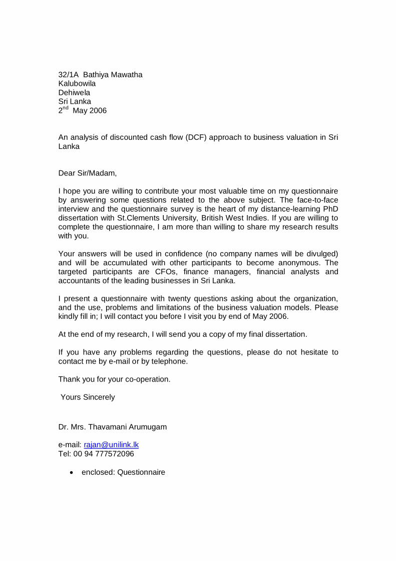
32/1A Bathiya Mawatha Kalubowila Dehiwela Sri Lanka 2nd May 2006 An analysis of discounted cash flow (DCF) approach to business valuation in Sri Lanka Dear Sir/Madam, I hope you are willing to contribute your most valuable time on my questionnaire by answering some questions related to the above subject. The face-to-face interview and the questionnaire survey is the heart of my distance-learning PhD dissertation with St.Clements University, British West Indies. If you are willing to complete the questionnaire, I am more than willing to share my research results with you. Your answers will be used in confidence (no company names will be divulged) and will be accumulated with other participants to become anonymous. The targeted participants are CFOs, finance managers, financial analysts and accountants of the leading businesses in Sri Lanka. I present a questionnaire with twenty questions asking about the organization, and the use, problems and limitations of the business valuation models. Please kindly fill in; I will contact you before I visit you by end of May 2006. At the end of my research, I will send you a copy of my final dissertation. If you have any problems regarding the questions, please do not hesitate to contact me by e-mail or by telephone. Thank you for your co-operation. Yours Sincerely Dr. Mrs. Thavamani Arumugam e-mail: [email protected] Tel: 00 94 777572096
enclosed: Questionnaire

Questionnaire
An analysis of discounted cash flow (DCF) approach to business valuation in Sri Lanka Part I
1) Type of business: ………………………………………………………
2) Issued share capital of your business: ……………………………
3) Annual turnover for the last 3 years:
2005/06 ………………………
2004/05 ………………………
2003/04 ………………………
4) Number of staff: ……………………
Part II
Please tick your answer:
5) What is the priority of your firm’s valuation technique?
1st 2nd 3rd
Asset based valuation …………. …………. …………
Discounted Cash Flow …………. …………. …………
Relative valuation …………. …………. …………
Others .………… …………. …………

6) Do you carry out SWOT analysis of your firm and incorporate the results when
you carry out future forecast of sales ?
Yes……….. No……….
7) What is the method you use to forecast your firm’s sales revenue for future?
Time trend Analysis ……………
Causal method ……………
Delphi method ……………
Others ……………
8) What is the method you use to estimate the terminal value of your firm?
Stable growth model …………….
Multiple approach …………….
Liquidation value …………….
9) What is the rate your firm use to calculate its cost of debt?
Rate at which the firm can borrow at today …………….
Corrected rate for tax benefit ……………..
Others ……………..
10) Which security does your firm use as risk-free rate?
Treasury bill rate ………………
Treasury bond rate ………………
11) What is the method your firm use to estimate risk premium of your firm?
Historical ………………
Implied ………………
12) Is sufficient data available for historical risk premium?
Yes………….. No……………
13) Is your firm exposed to additional country risk?
Yes………….. No……………
14) What is the method your firm use to estimate the risk factor beta of your firm?
Regression of stock return method …………….
Standard deviation in stock prices instead of regression …………….
Accounting earnings or revenues ……………
Others ……………
15) What is the method your firm use to calculate the cost of equity?
Capital asset pricing model CAPM ……………
Arbitrage pricing model ……………
Multifactor model ……………
Others …………...
16) What is the method your firm use to calculate the discount rate to apply in
discounted cash flow valuation (DCF)?
Weighted average cost of capital WACC …………..
Cost of equity …………...
17) What is the percentage of accuracy you have achieved in using DCF
valuation technique in your firm?
41 – 50% ……….. 51 – 60% ………. 61 – 70% ……….
71 – 80% ……….. 81 – 90% ……….. 91 – 100% ………

Part III
18) What type of problems have you faced with when using the valuation models
and how do these problems affect your firm’s final decisions?
………………………………………………………………………………………….
………………………………………………………………………………………….
………………………………………………………………………………………….
………………………………………………………………………………………….
………………………………………………………………………………………….
19) What are the limitations of the valuation model your firm use?
…………………………………………………………………………………………
…………………………………………………………………………………………
…………………………………………………………………………………………
…………………………………………………………………………………………
20) Any other comments.
………………………………………………………………………………………….
………………………………………………………………………………………….
………………………………………………………………………………………….
………………………………………………………………………………………….
………………………………………………………………………………………….