Using SmartXplorer to achieve timing closure

The main purpose of Xilinx’ SmartXplorer is to achieve timing closure where the default

place-and-route (PAR) strategy results in a “near miss”. It can be much more convenient than

attempting to manually floorplan the design, and with a lot less hands-on effort. In this document

I provide a walkthrough for using SmartXplorer, through to a programmable binary file.

SmartXplorer is an appropriate tool if you’ve optimised your design’s latencies as best you

can, however the design still hasn’t quite met timing. Very large timing scores, '105, indicate

serious problems in your design and you should look at adding or removing latency depending on

what the timing report identifies as the worst areas of negative slack. However, a timing score of

∼few×104 indicates the design is quite close to achieving closure. Indeed, you may even make

the situation worse if you haphazardly add pipelines, especially since the timing report can be

misleading.

SmartXplorer is essentially a brute-force method to achieve timing closure. Its method is to

cycle through the seven general PAR strategies, achieving a zero-score if it can. If not, there are

further low-level optimisations that can be made which are also cycled through, up to the runtime

limits set by the user.

Using SmartXplorer

In this section I take an example for three general regimes in which I’ve found SmartXplorer’s

effectiveness to be distinct. The first regime is a small (4096-channel) spectrometer design which

has, unbelievably, missed timing after running asper_xps. The second is a 16384-channel

spectrometer design, and the third a 32768-channel, 8-tap, two-polarisation spectrometer which

tested the limits of SmartXplorer’s capabilities.

1

Setup

On a Linux machine, start ISE in the normal way. If you’ll be using SmartXplorer often, I

recommend adding a command line shortcut in your ~bashr /~ shr file. The first step is to

click File and then New Proje t. This will start the wizard. At this point you must select

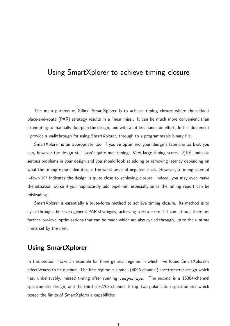
a project directory, in much the same way you would with PlanAhead. I recommend a project

directory in the sub-directory created by asper_xps intially, for convenience, as in Figure 1.

There are a couple of scenarios in which you might not want to do this, which I will discuss in

Tips and Tricks.

Figure 1: Step 1 is to create the project directory. Pick a simple, obvious directory name in theexisting project directory for convenience.

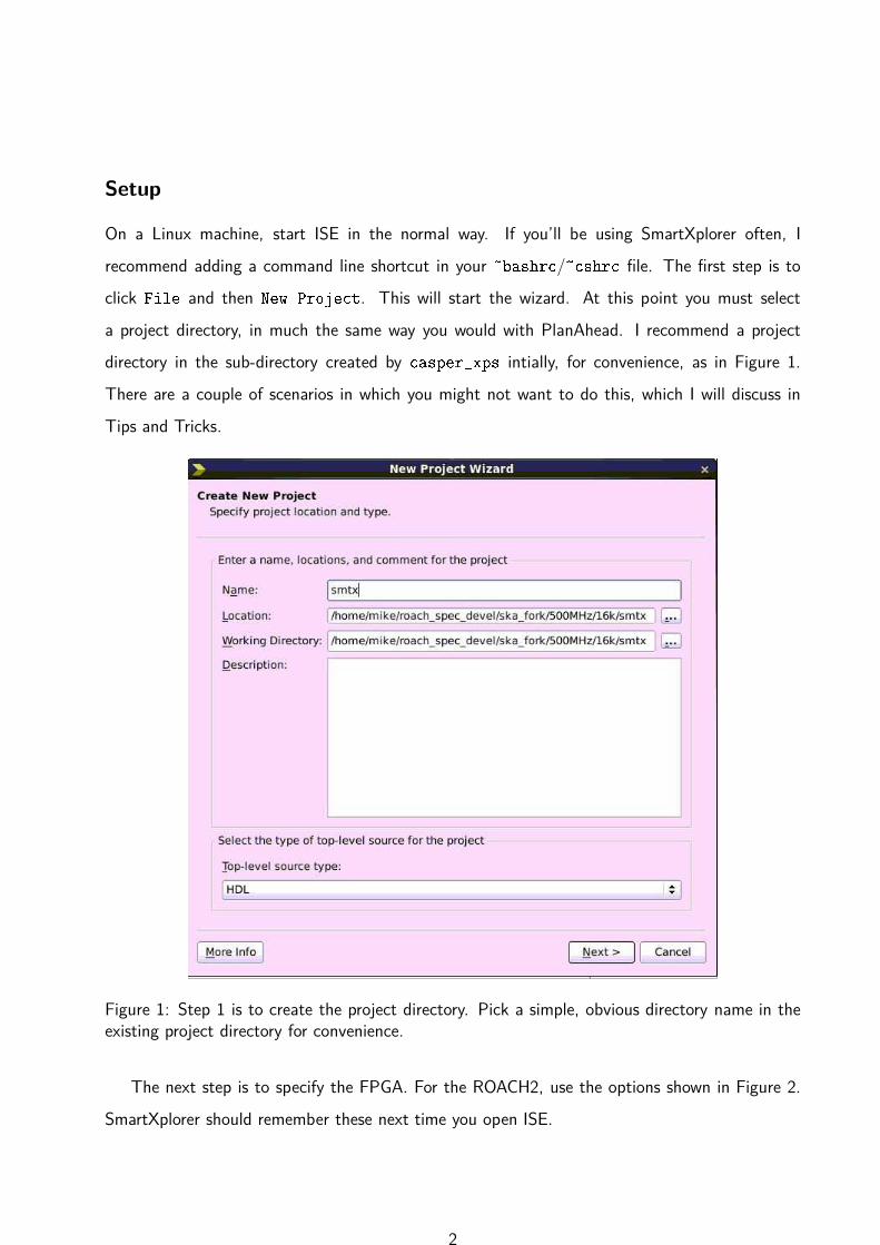
The next step is to specify the FPGA. For the ROACH2, use the options shown in Figure 2.

SmartXplorer should remember these next time you open ISE.

2

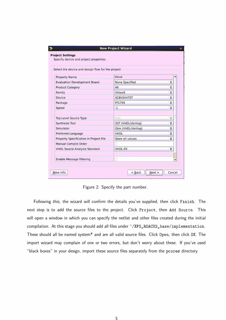
Figure 2: Specify the part number.

Following this, the wizard will confirm the details you’ve supplied, then click Finish. The

next step is to add the source files to the project. Click Proje t, then Add Sour e. This

will open a window in which you can specify the netlist and other files created during the initial

compilation. At this stage you should add all files under ~/XPS_ROACH2_base/implementation.

These should all be named system* and are all valid source files. Click Open, then click OK. The

import wizard may complain of one or two errors, but don’t worry about these. If you’ve used

“black boxes” in your design, import these source files separately from the p ores directory.

3

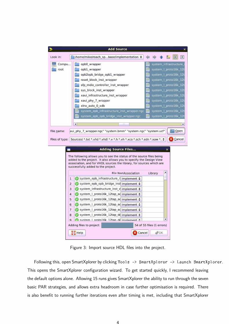
Figure 3: Import source HDL files into the project.

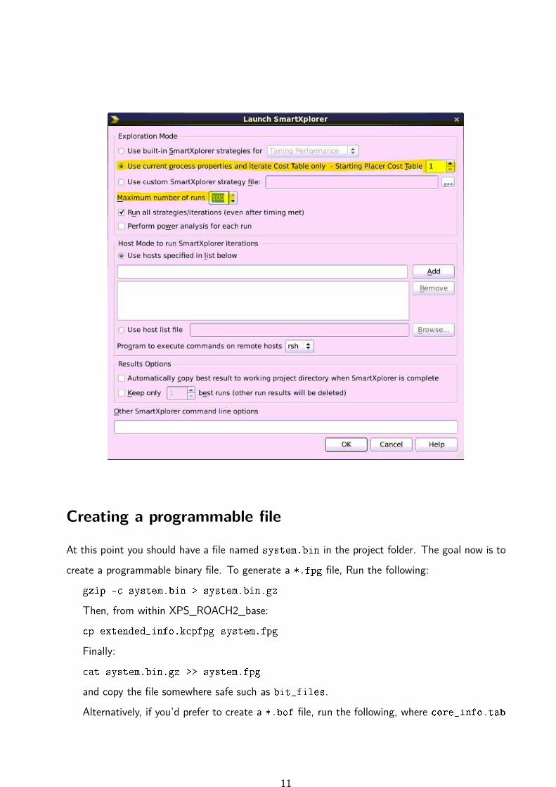
Following this, open SmartXplorer by clicking Tools -> SmartXplorer -> Laun h SmartXplorer.

This opens the SmartXplorer configuration wizard. To get started quickly, I recommend leaving

the default options alone. Allowing 15 runs gives SmartXplorer the ability to run through the seven

basic PAR strategies, and allows extra headroom in case further optimisation is required. There

is also benefit to running further iterations even after timing is met, including that SmartXplorer

4

may find a better solution with greater slack or by utilising fewer resources. Click OK to start the

process. This will likely take several hours!

Figure 4: The SmartXplorer configuration wizard.

Multi-threading

SmartXplorer is single-threaded by default, but accessing its multi-threading capabilities is easy.

The first step is to find out what your machine’s name is. Type hostname in a terminal, to obtain

this. In my case it is roa h-workstation. To have SmartXplorer run on multiple cores, each

instance must be added as a host in the SmartXplorer configuration wizard. If, for example, you

want to run three threads, type the machine name into the list of hosts three times, as below.

For reference, I use a workstation PC with a six-core CPU with hyperthreading, and 64 GB RAM.

For overnight runs I will typically run five threads, or if I’m running SmartXplorer while doing

5

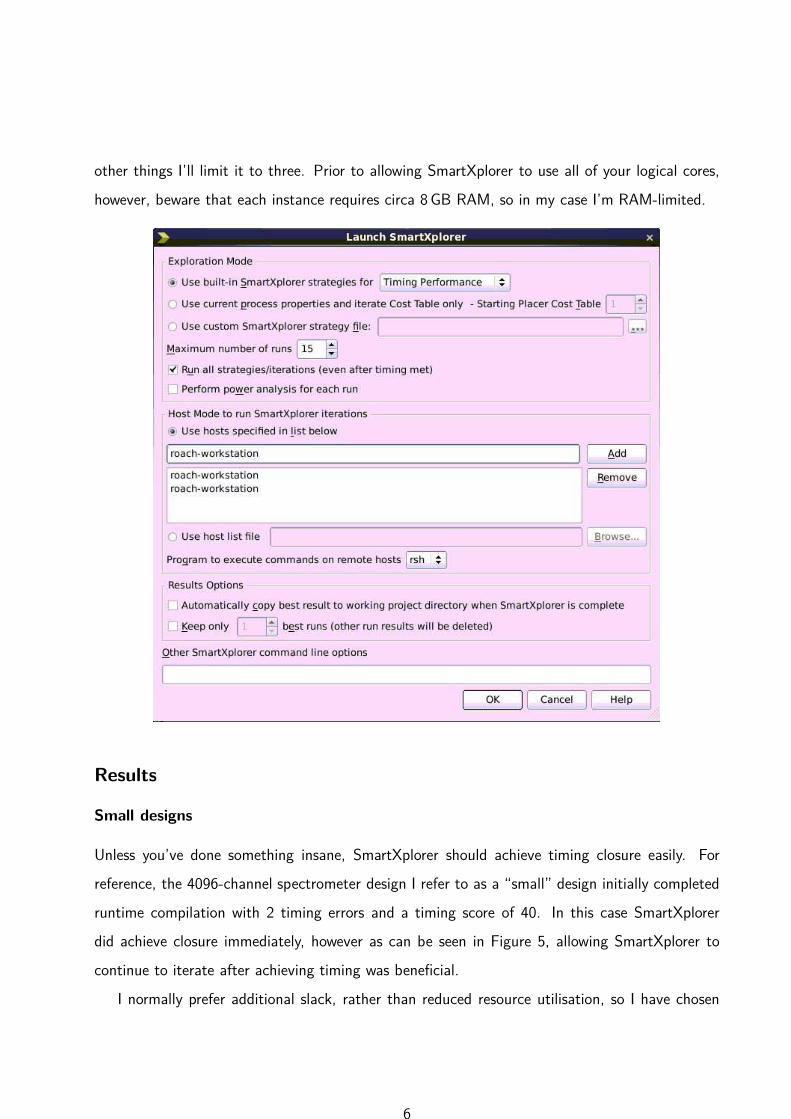
other things I’ll limit it to three. Prior to allowing SmartXplorer to use all of your logical cores,

however, beware that each instance requires circa 8 GB RAM, so in my case I’m RAM-limited.

Results

Small designs

Unless you’ve done something insane, SmartXplorer should achieve timing closure easily. For

reference, the 4096-channel spectrometer design I refer to as a “small” design initially completed

runtime compilation with 2 timing errors and a timing score of 40. In this case SmartXplorer

did achieve closure immediately, however as can be seen in Figure 5, allowing SmartXplorer to

continue to iterate after achieving timing was beneficial.

I normally prefer additional slack, rather than reduced resource utilisation, so I have chosen

6

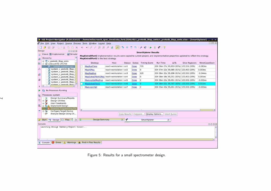
Figure 5: Results for a small spectrometer design.

7

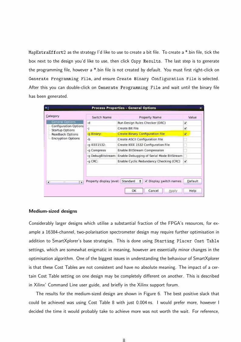
MapExtraEffort2 as the strategy I’d like to use to create a bit file. To create a *.bin file, tick the

box next to the design you’d like to use, then click Copy Results. The last step is to generate

the programming file, however a *.bin file is not created by default. You must first right-click on

Generate Programming File, and ensure Create Binary Configuration File is selected.

After this you can double-click on Generate Programming File and wait until the binary file

has been generated.

Medium-sized designs

Considerably larger designs which utilise a substantial fraction of the FPGA’s resources, for ex-

ample a 16384-channel, two-polarisation spectrometer design may require further optimisation in

addition to SmartXplorer’s base strategies. This is done using Starting Pla er Cost Table

settings, which are somewhat enigmatic in meaning, however are essentially minor changes in the

optimisation algorithm. One of the biggest issues in understanding the behaviour of SmartXplorer

is that these Cost Tables are not consistent and have no absolute meaning. The impact of a cer-

tain Cost Table setting on one design may be completely different on another. This is described

in Xilinx’ Command Line user guide, and briefly in the Xilinx support forum.

The results for the medium-sized design are shown in Figure 6. The best positive slack that

could be achieved was using Cost Table 8 with just 0.004 ns. I would prefer more, however I

decided the time it would probably take to achieve more was not worth the wait. For reference,

8

this design initially completed runtime compilation with 10 timing errors and a timing score of

486. Note in the Figure how substantially small changes in the optimisation settings can affect

the timing score.

Large designs

Designs which use a large majority of the FPGA’s resources, for example a 32768-channel, 8-

tap, two-polarisation spectrometer will have varying results using SmartXplorer. I have observed

designs of this size with a timing score ≈100 make no improvement despite days of running in

SmartXplorer, where designs which missed timing closure by much larger margins were closed in

SmartXplorer. The biggest factor impacting the effectiveness of SmartXplorer for designs of this

size is the amount you constrain your design, either by using too few or too many pipelines. The

worst example I have of this is a design which took nearly a week to achieve closure. The design

initially failed timing with 18 errors and a score of 6692. In this instance, the initial number of

runs I had allowed SmartXplorer to use were insufficient, so I utilised a further option which I will

now describe.

Where the initial number of runs is insufficient, SmartXplorer has the option to take the

best current case, and iterate through Cost Tables for up to 100 runs. To access this, first

copy the results from the best current case as before. Next, launch SmartXplorer via Tools ->

SmartXplorer -> Laun h SmartXplorer. This time, click on the second radio button, and

adjust the starting Cost Table to the current value, plus one. I recommend setting the number

of runs as high as you can afford. Finally, start SmartXplorer again by clicking OK.

Hopefully timing will be met eventually. My results are shown in Figure 7. You can see that

timing was met at Cost Table 33 after a few days of running, and allowed to run further in the

hope that a better solution could be found (it wasn’t).

9

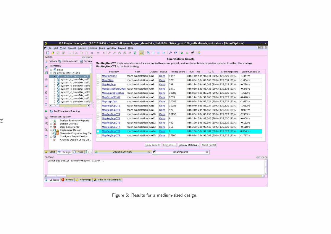
Figure 6: Results for a medium-sized design.

10

Creating a programmable file

At this point you should have a file named system.bin in the project folder. The goal now is to

create a programmable binary file. To generate a *.fpg file, Run the following:

gzip - system.bin > system.bin.gz

Then, from within XPS_ROACH2_base:

p extended_info.k pfpg system.fpg

Finally:

at system.bin.gz >�> system.fpg

and copy the file somewhere safe such as bit_files.

Alternatively, if you’d prefer to create a *.bof file, run the following, where ore_info.tab

11

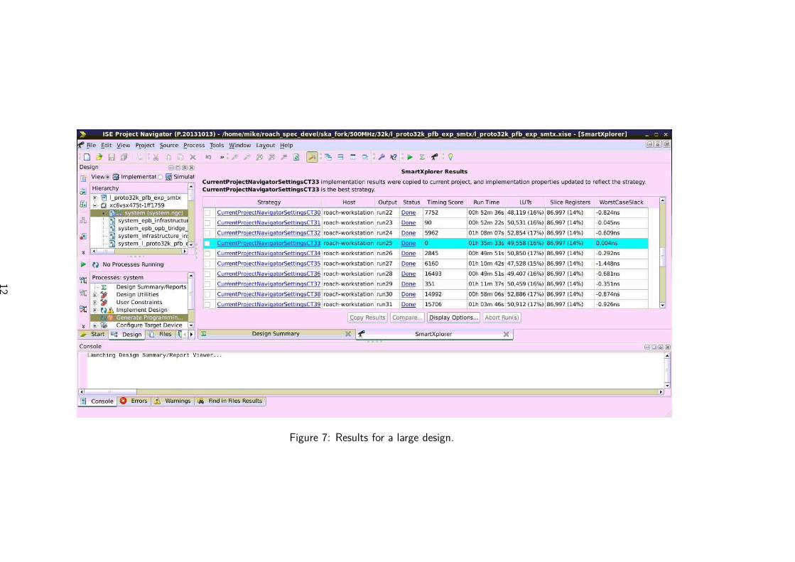
Figure 7: Results for a large design.

12

is found in XPS_ROACH2_base/:

mkbof -o system.bof -s ore_info.tab -t 3 system.bit

Tips and Tricks

Earlier I mentioned that there were a couple of scenarios in which you might not want a SmartX-

plorer project folder inside the folder created during your initial run of asper_xps. These

scenarios are as follows:

1. Optimising multiple strategies

SmartXplorer will always choose to optimise Cost Tables for the best result from the seven base

strategies. I find this a poor approach since, in the case that two or more of the base strategies

give similar results, the other two are ignored. In this case, you can start several instances of

SmartXplorer and try iterating the Cost Tables for the other two instead. In order to do this,

you must create a new project folder for each strategy, and copy everything from the original

SmartXplorer run to the new folders. Rename the folders to reflect the strategies you’re optimising,

and also rename the *.xise project file itself. It is critical that you do not start each of the new

processes while the initial project is still running. This is because the *.xise file refers to a

particular process as SmartXplorer tries to open the most recent project on startup, which could

cause serious problems with any jobs still running associated with that particular file.

2. Running SmartXplorer and casper_xps

There may be occasions in which you were close enough to meeting timing with asper_xps

that you want to alter your design slightly, but at the same time want to run the current design

configuration in SmartXplorer in case your alterations make things worse. In this case, you should

copy the entire folder which asper_xps created, into a new folder into which you then create

your SmartXplorer project folder. This avoids SmartXplorer trying to call netlist files which are

being continually overwritten as the toolflow runs.

13