– using Propensity scores

Shelley Fordred Victor Kiri

Knut Mueller

1

� Introduction – Matching and Propensity Scores � Study Design � How it was done – Variable Selection and

PROC LOGISTIC � Matching approach � Results of matching � Conclusion � Acknowledgements

2

�  The aim of this study was to compare the direct healthcare cost of treating patients with epilepsy on a particular class of drugs from treatment A against another class of drugs from treatment B, using the propensity score-matched cohort methodology on a 1:1 basis.

�  Matching - is where exposed subjects are matched to unexposed based on their baseline characteristics - limitations : large sample size, large number of confounders - advantages: reduce confounding �  Propensity Score: the probability of the patient being

prescribed treatment B on the basis of the selected covariates at baseline

3

4

CPRD subset of patients with a diagnosis of epilepsy and one prescription of a drug from class A or class B during the selection period .

4,889

Index Date

Index Drug

Unmatched Treatment A

2,752

Unmatched Treatment B

2,137

Propensity Score

 

Matched 1:1

Matched Treatment A

951

Matched Treatment B

951

 

Pre-Index - 1 Year

 

� Selection of the baseline Characteristics including the epilepsy related clinical variables.

- All of the Baseline Characteristics variables were selected. � Selection of the Comorbidities and

Concomitant medication - If either the treatment differences were statistically different with a p- value of <0.05 or if the comorbidity or the medication had an incidence of >1% in either treatment . - 318 variables used for matching

5

�  Propensity Score Creation using PROC LOGISTIC

proc logistic data=fullbase; class &varlistc/order=freq param=ref ref=first; model indextype (event=“TRTB”)=&varlist; output out=prop_score p=prop_score; run; PROC LOGISTIC - fits the linear logistic regression models for binary (Y’s , N’s) or ordinal response data by the method of maximum likelihood - modelled the likelihood of a patient receiving treatment B using ‘(event=TRTB)’ and the numeric and character confounding variables in the &varlist, the character variables are specified in the class statement - param= option defines the parameterisation and uses the variable ref which specifies the baseline variable in ‘ref=first’ - prop_score is the output dataset and p= names the variable containing the predicted probabilities i.e. the propensity score.

6

� Propensity Score was transformed to logit(PS)= log(prop_score/(1-prop_score));

� Caliper = 0.2*std(logitps) � Matching carried out using a validated in-

house macro which applied the Caliper method without replacement.

� Within each age range subjects were matched on their logit(PS)+/- caliper

TREATED LOGIT(PS) (21-30 YRS)

+/- CALIPER CONTROL LOGIT(PS) (21-30 YRS)

7

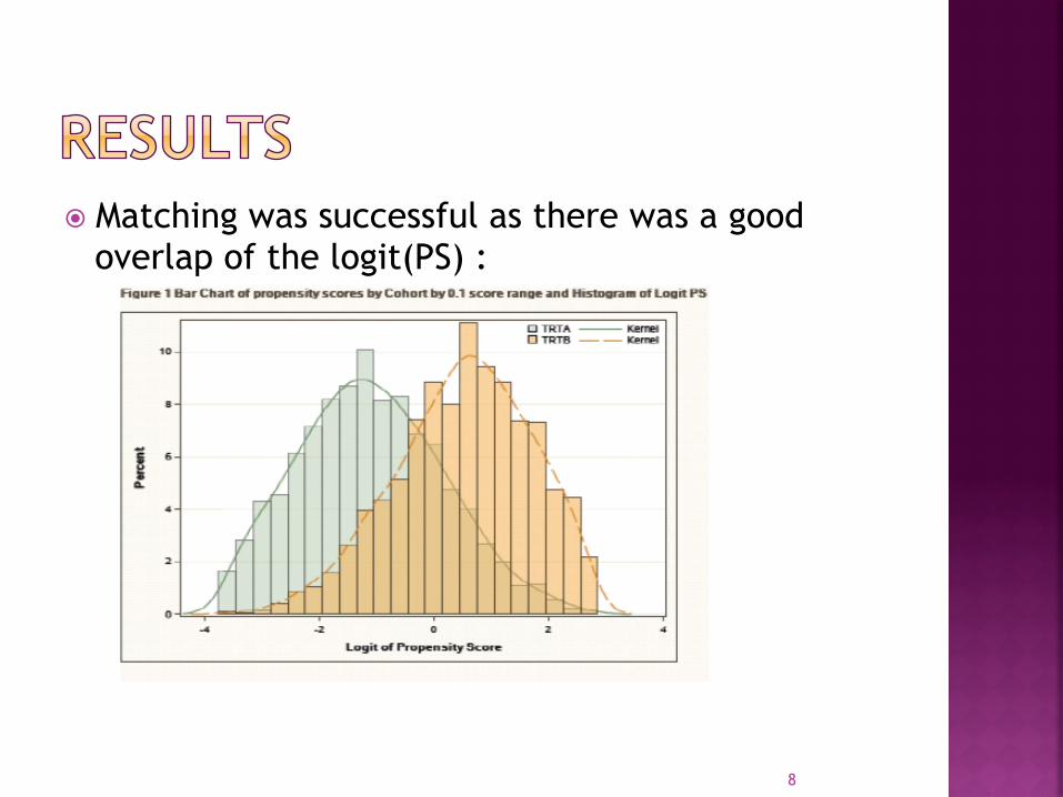
� Matching was successful as there was a good overlap of the logit(PS) :

8

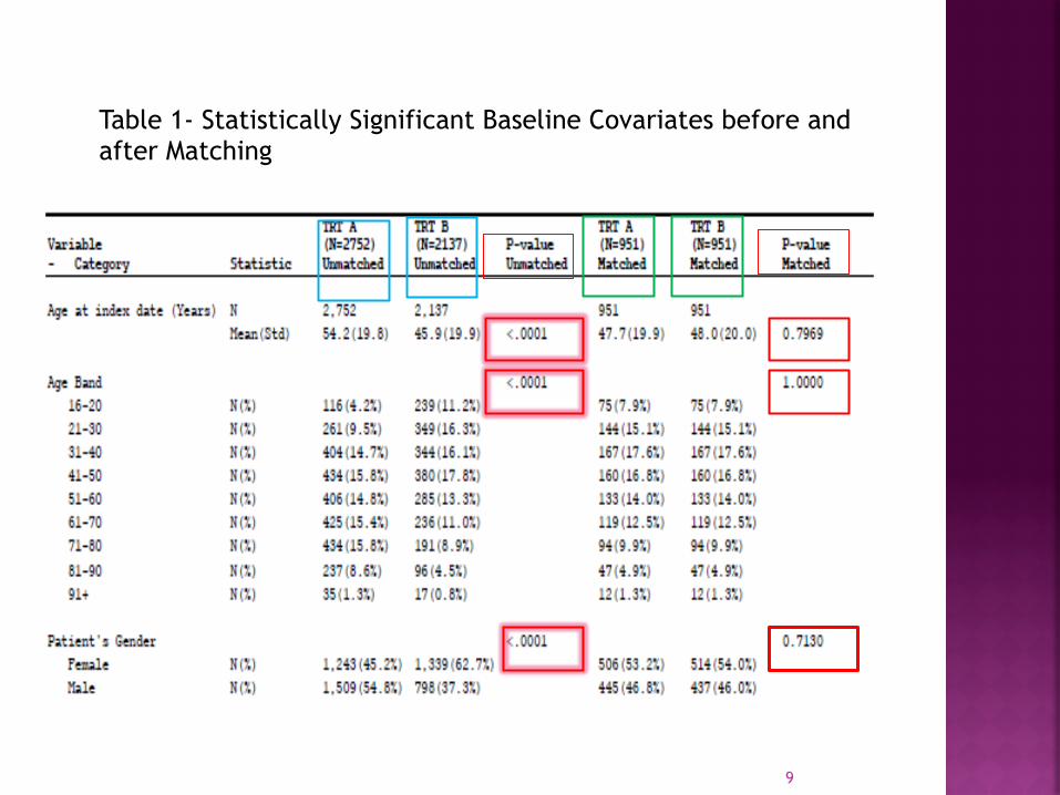
Table 1- Statistically Significant Baseline Covariates before and after Matching

9

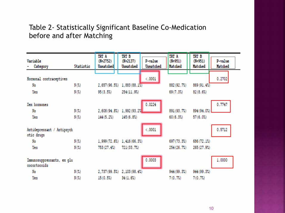
Table 2- Statistically Significant Baseline Co-Medication before and after Matching

10

� Main challenges (Programmer’s perspective): — Decision on best matching method to use — Guidance on which covariates should be selected

for the propensity score model — May have to advise team on variable selection via

exploratory analysis and prior experience — Team decision on variable selection is final!

� Matching successfully implemented: 1902 matched subjects out of 4,889

� The two groups were balanced on all variables � Confident that the cost results were based on

subjects with the same baseline characteristics and confounding reduced.

11

I would like to thank Knut Mueller , Victor Kiri and John Logan with helping me to write this paper J

12