Computational Reality XI

Using complex geometries

B. Emek Abali, Ntsah Donald @ LKM - TU Berlin

Abstract

Simple geometries in the dolfin packages are useful for many scientific problem. However, an engineerneeds to compute quite often more complicated structures, in other words, reality is more than a box!

1 Import and convert

Day starts with a digital clock alarm and goes on with usage of mp3 player, mobile phone and laptop. Theyare all built of similiar devices like transistors, resistors and microchips, which are placed on a circuit board(mostly green or blue) and connected via copper pathways. There exists many different production method-ologies, however, as a common point, different materials are attached together, as to be seen in figure 1. Thetask of the board is to transfer (conduct) electric signals between chip and other elements. This produces heatenergy due to electrical resistance. The board consists of different materials, with different material properties.Under temperature rise caused by the heat energy, material tries to expand, in terms of its expansion coefficientα. The elements are fixed together by soldering. Different materials with different expansion coefficients, re-strict reciprocally while they are connected and thus occur (thermally induced) stresses in the structure. Thesestresses change dynamically and the material get fatigue, caused by thermal fluctuations due to the usage ofthe electronic device. Over a period of time, fatigueness results of weakening the stiffness and yields to rupture.This is a highly complicated analysis and in many cases only numerically possible.

Here we want to make an introduction to the topic and only show how to get off the first milestone, namely im-porting a complex model with different materials into FEniCS by using the mesh converter script abaqus2xml.pyunder http://www.lkm.tu-berlin.de/ComputationalReality/ . We skip a detailed tutorial about how to model sucha geometry and mesh in Abaqus as seen1 in figure 2. Only three-dimensional elements with four nodes are ac-

1for a more detailed instruction, you may visit the course: Projekt zur finiten Elementmethode in our chair http://www.lkm.tu-berlin.de/

Figure 1: Circuit board with microchip, transistors and resistance

1

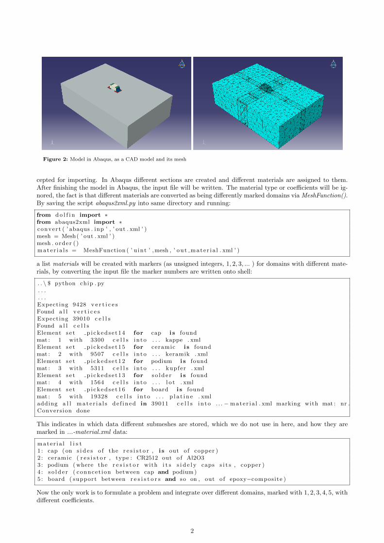
Figure 2: Model in Abaqus, as a CAD model and its mesh

cepted for importing. In Abaqus different sections are created and different materials are assigned to them.After finishing the model in Abaqus, the input file will be written. The material type or coefficients will be ig-nored, the fact is that different materials are converted as being differently marked domains via MeshFunction().By saving the script abaqus2xml.py into same directory and running:

from d o l f i n import ∗from abaqus2xml import ∗convert ( ’ abaqus . inp ’ , ’ out . xml ’ )mesh = Mesh( ’ out . xml ’ )mesh . order ( )m a t e r i a l s = MeshFunction ( ’ u int ’ ,mesh , ’ ou t mate r i a l . xml ’ )

a list materials will be created with markers (as unsigned integers, 1, 2, 3, ... ) for domains with different mate-rials, by converting the input file the marker numbers are written onto shell:

. . \ $ python chip . py

. . .

. . .Expecting 9428 v e r t i c e sFound a l l v e r t i c e sExpecting 39010 c e l l sFound a l l c e l l sElement s e t p i c k e d s e t 1 4 for cap i s foundmat : 1 with 3300 c e l l s i n to . . . kappe . xmlElement s e t p i c k e d s e t 1 5 for ceramic i s foundmat : 2 with 9507 c e l l s i n to . . . keramik . xmlElement s e t p i c k e d s e t 1 2 for podium i s foundmat : 3 with 5311 c e l l s i n to . . . kupfer . xmlElement s e t p i c k e d s e t 1 3 for s o l d e r i s foundmat : 4 with 1564 c e l l s i n to . . . l o t . xmlElement s e t p i c k e d s e t 1 6 for board i s foundmat : 5 with 19328 c e l l s i n to . . . p l a t i n e . xmladding a l l m a t e r i a l s de f ined in 39011 c e l l s i n to . . . − mate r i a l . xml marking with mat : nr .Conversion done

This indicates in which data different submeshes are stored, which we do not use in here, and how they aremarked in ...-material.xml data:

mate r i a l l i s t1 : cap ( on s i d e s o f the r e s i s t o r , i s out o f copper )2 : ceramic ( r e s i s t o r , type : CR2512 out o f Al2O33 : podium ( where the r e s i s t o r with i t s s i d e l y caps s i t s , copper )4 : s o l d e r ( conncet ion between cap and podium )5 : board ( support between r e s i s t o r s and so on , out o f epoxy−composite )

Now the only work is to formulate a problem and integrate over different domains, marked with 1, 2, 3, 4, 5, withdifferent coefficients.

2

2 Example problem

We use the most simple example, stationary linear elasticity. Elastic part of the strain tensor is given:

εelij = εij − εth

ij , εij =1

2

(∂ui∂xj

+∂uj∂xi

), εth

ij = δijα(T − Tref.) , (1)

where ui denotes the displacement field which is sought after. Strain-stress tensors satisfy Hookes law forisotropic materials:

σij = Cijklεelkl , Cijkl = λδijδkl + µ(δikδjl + δilδjk) ,

λ =Eν

(1 + ν)(1 − 2ν)=

2Gν

(1 − 2ν), µ =

E

2(1 + ν)= G . (2)

Then starting from the balance of momentum

ρvi −∂σij∂xj

= ρfi , (3)

and assuming stationarity, neglecting gravity, using small displacements2 ui < 0.02Xi that

xi = ui +Xi , xi ≈ Xi ,∂xi∂Xj

= δij , J = det( ∂xi∂Xj

)= 1 (4)

hold, using only Dirichlet conditions, we reach to the variational form in material coordinates (for details cf.to part I and part II): ∫

Ω

∂wi

∂Xjσij dx = 0 . (5)

Here, we have five different materials. Actually they all have different characteristics and should not be modeledsimply elastically. However, in this part we only want to demonsrate importing and solving a CAD model withmany materials, thus modeling them all elastic with different coefficients. Stress is a function of variatingcoefficients and the form becomes:∫

Ω1

∂wi

∂Xjσij(E1, ν1, α1) dx+

∫Ω2

∂wi

∂Xjσij(E2, ν2, α2) dx+

∫Ω3

∂wi

∂Xjσij(E3, ν3, α3) dx

+

∫Ω4

∂wi

∂Xjσij(E4, ν4, α4) dx+

∫Ω5

∂wi

∂Xjσij(E5, ν5, α5) dx = 0 . (6)

Shape of geometry changes due to temperature rise. Again we make a crude assumption that temperaturechanges uniformly in whole structure (for a complete solution cf. part IX). Shape change can be measured bystored energy:

ψ =

∫Ω

e dx =

∫Ω

σij dεel.ij . (7)

A subtle point by programming is that u=Function() defines an object u which is used in sigma(..) and thencalculated via solve(..). Logically, one may try to use again sigma(..) to evaluate the energy over domain, butthis will not work, since it points on the object not to the values of it. Therefore we solve another problem,with the usage of calculated u found energy density

e = σijεel.ij = εel.

ij Cijklεel.kl = λεel.

kkεel.ll + 2µεel.

ij εel.ij . (8)

In theory of elasticity, starting directly from this energy definition is quite popular (cf. part III). Here weintroduce it as a measure of deformation and also fatigue, as seen in figure 3. Displacements are continuous butthey build different stresses and strains, thus discontinuous energy field between different materials. Hence forfatigue analysis, the utilized material models and their coefficients are at most importance.

2many engineering materials like steel, aluminium, magnesium, copper behave elastically up to strain 2%

3

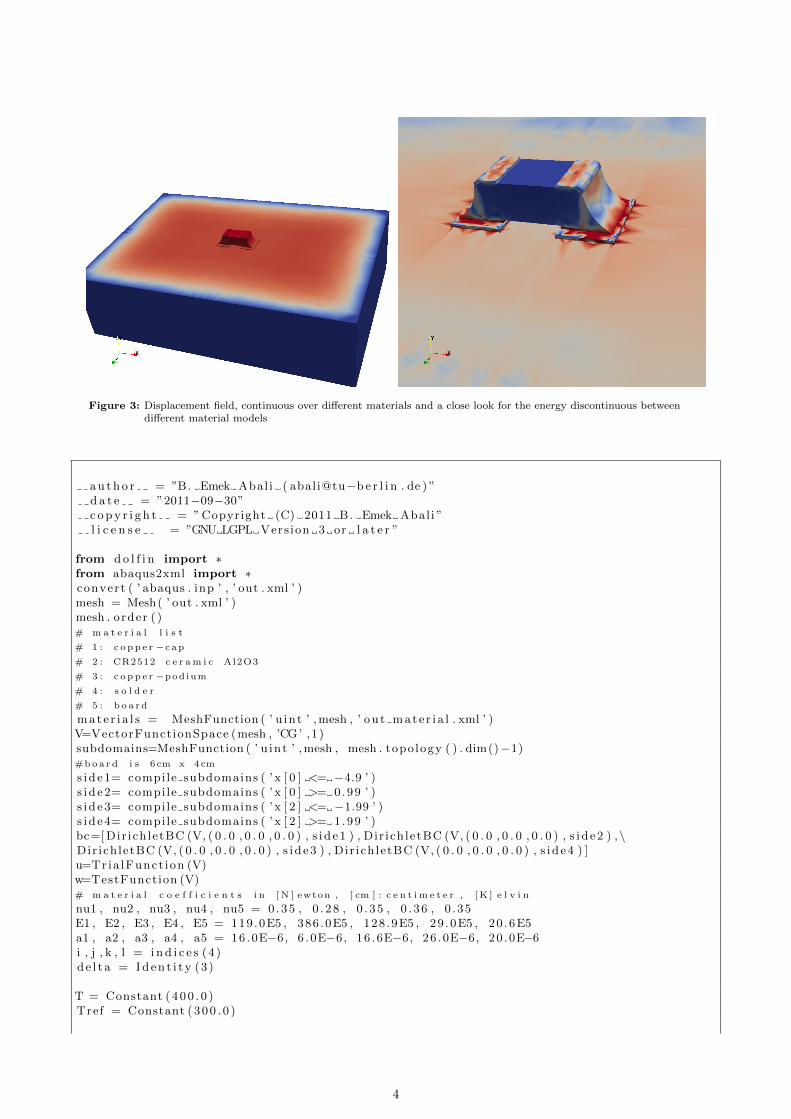
Figure 3: Displacement field, continuous over different materials and a close look for the energy discontinuous betweendifferent material models

a u t h o r = ”B. Emek Abal i ( abali@tu−b e r l i n . de ) ”d a t e = ”2011−09−30”c o p y r i g h t = ” Copyright (C) 2011 B. Emek Abal i ”l i c e n s e = ”GNU LGPL Vers ion 3 or l a t e r ”

from d o l f i n import ∗from abaqus2xml import ∗convert ( ’ abaqus . inp ’ , ’ out . xml ’ )mesh = Mesh( ’ out . xml ’ )mesh . order ( )# m a t e r i a l l i s t

# 1 : c o p p e r −c a p

# 2 : CR2512 c e r a m i c Al2O3

# 3 : c o p p e r −pod ium

# 4 : s o l d e r

# 5 : b o a r d

m a t e r i a l s = MeshFunction ( ’ u int ’ ,mesh , ’ ou t mate r i a l . xml ’ )V=VectorFunctionSpace (mesh , ’CG’ ,1 )subdomains=MeshFunction ( ’ u int ’ ,mesh , mesh . topo logy ( ) . dim()−1)#b o a r d i s 6 cm x 4cm

s i d e1= compile subdomains ( ’ x [ 0 ] <= −4.9 ’ )s i d e2= compile subdomains ( ’ x [ 0 ] >= 0.99 ’ )s i d e3= compile subdomains ( ’ x [ 2 ] <= −1.99 ’ )s i d e4= compile subdomains ( ’ x [ 2 ] >= 1.99 ’ )bc=[ Dir ichletBC (V, ( 0 . 0 , 0 . 0 , 0 . 0 ) , s i d e1 ) , Dir ichletBC (V, ( 0 . 0 , 0 . 0 , 0 . 0 ) , s i d e2 ) ,\Dir ichletBC (V, ( 0 . 0 , 0 . 0 , 0 . 0 ) , s i d e3 ) , Dir ich letBC (V, ( 0 . 0 , 0 . 0 , 0 . 0 ) , s i d e4 ) ]u=Tr ia lFunct ion (V)w=TestFunction (V)# m a t e r i a l c o e f f i c i e n t s i n [ N ] ewton , [ cm ] : c e n t i m e t e r , [ K ] e l v i n

nu1 , nu2 , nu3 , nu4 , nu5 = 0 .35 , 0 . 28 , 0 . 35 , 0 . 36 , 0 .35E1 , E2 , E3 , E4 , E5 = 119 .0E5 , 386 .0E5 , 128 .9E5 , 29 .0E5 , 20 .6E5a1 , a2 , a3 , a4 , a5 = 16 .0E−6, 6 . 0E−6, 16 .6E−6, 26 .0E−6, 20 .0E−6i , j , k , l = i n d i c e s (4 )d e l t a = I d e n t i t y (3 )

T = Constant ( 4 0 0 . 0 )Tref = Constant ( 3 0 0 . 0 )

4

e p s t o t a l = a s t e n s o r ( 0 . 5∗ ( u [ i ] . dx ( j ) + u [ j ] . dx ( i ) ) , [ i , j ] )

def eps therm ( alpha ) : return a s t e n s o r ( alpha ∗(T−Tref )∗ d e l t a [ i , j ] , [ i , j ] )

def C(E, nu ) :G = E/(2 .0∗ (1 .0+ nu ) )lmb , mu = 2.0∗G∗nu/(1.0−2.0∗nu ) , Greturn a s t e n s o r ( lmb∗ d e l t a [ i , j ]∗ d e l t a [ k , l ] + \mu∗ d e l t a [ i , k ]∗ d e l t a [ j , l ] + mu∗ d e l t a [ i , l ]∗ d e l t a [ j , k ] , [ i , j , k , l ] )

def sigma (E, nu , a ) : return a s t e n s o r (C(E, nu ) [ i , j , k , l ] ∗ ( e p s t o t a l [ k , l ]−\eps therm ( a ) [ k , l ] ) , [ i , j ] )

Form = w[ i ] . dx ( j )∗ sigma (E1 , nu1 , a1 ) [ j , i ]∗ dx (1 ) \+ w[ i ] . dx ( j )∗ sigma (E2 , nu2 , a2 ) [ j , i ]∗ dx (2 ) \+ w[ i ] . dx ( j )∗ sigma (E3 , nu3 , a3 ) [ j , i ]∗ dx (3 ) \+ w[ i ] . dx ( j )∗ sigma (E4 , nu4 , a4 ) [ j , i ]∗ dx (4 ) \+ w[ i ] . dx ( j )∗ sigma (E5 , nu5 , a5 ) [ j , i ]∗ dx (5 )

l e f t=l h s (Form)r i g h t=rhs (Form)A = assemble ( l e f t , c e l l doma in s=mater ia l s , mesh=mesh )b = assemble ( r i ght , c e l l doma in s=mater ia l s , mesh=mesh )

for cond i t i on in bc :cond i t i on . apply (A, b)

u=Function (V)s o l v e (A, u . vec to r ( ) , b , ’ lu ’ )

f i l e=F i l e ( ’ complex geo d i sp . pvd ’ )f i l e << u

#u i s c a l c u l a t e d , i t i s now a g i v e n f u n c t i o n

en = FunctionSpace (mesh , ’CG’ , 1)e = Tr ia lFunct ion ( en )q = TestFunction ( en )

#we h a v e t o d e f i n e i t a g a i n , u i s n o t a T r i a l F u n c t i o n ( )

# i t i s now a g i v e n F u n c t i o n ( )

def eps mech ( a ) : return a s t e n s o r ( 0 . 5∗ ( u [ i ] . dx ( j ) + \u [ j ] . dx ( i ))−a ∗(T−Tref )∗ d e l t a [ i , j ] , [ i , j ] )

def energy (E, nu , a ) :G = E/(2 .0∗ (1 .0+ nu ) )lmb , mu = 2.0∗G∗nu/(1.0−2.0∗nu ) , Greturn lmb∗ eps mech ( a ) [ k , k ]∗ eps mech ( a ) [ l , l ] + \2 .0∗mu∗ eps mech ( a ) [ i , j ]∗ eps mech ( a ) [ i , j ]

#a way o f f i n d i n g e= e n e r g y i s t o s o l v e ( e− e n e r g y ) ∗ q ∗ dx

e n l e f t = e∗q∗dx (1 ) + e∗q∗dx (2) + e∗q∗dx (3) + e∗q∗dx (4 ) + e∗q∗dx (5)e n r i g h t = q∗ energy (E1 , nu1 , a1 )∗dx (1) \

+ q∗ energy (E2 , nu2 , a2 )∗dx (2) \+ q∗ energy (E3 , nu3 , a3 )∗dx (3) \+ q∗ energy (E4 , nu4 , a4 )∗dx (4) \+ q∗ energy (E5 , nu5 , a5 )∗dx (5)

Aen = assemble ( e n l e f t , c e l l doma in s=mater ia l s , mesh=mesh )ben = assemble ( en r i gh t , c e l l doma in s=mater ia l s , mesh=mesh )e=Function ( en )s o l v e (Aen , e . vec to r ( ) , ben , ’ lu ’ )

5

f i l e=F i l e ( ’ complex geo energy . pvd ’ )f i l e << e

#−−−−−−−−−−−−−−−−−−−−−−−−−−−−−−−−−−−−−−−−−−−−−−−−−−−−−−−−

6