use of r as a toolbox for mathematical statistics explorationww2.amstat.org/misc/useofr.pdf · use...

Use of R as a Toolbox for Mathematical Statistics ExplorationNicholas J. HORTON, Elizabeth R. BROWN, and Linjuan QIAN

The R language, a freely available environment for statisticalcomputing and graphics is widely used in many fields. This“expert-friendly” system has a powerful command languageand programming environment, combined with an active usercommunity. We discuss how R is ideal as a platform to sup-port experimentation in mathematical statistics, both at the un-dergraduate and graduate levels. Using a series of case studiesand activities, we describe how R can be used in a mathemati-cal statistics course as a toolbox for experimentation. Examplesinclude the calculation of a running average, maximization ofa nonlinear function, resampling of a statistic, simple Bayesianmodeling, sampling from multivariate normal, and estimation ofpower. These activities, often requiring only a few dozen linesof code, offer students the opportunity to explore statistical con-cepts and experiment. In addition, they provide an introductionto the framework and idioms available in this rich environment.

KEY WORDS: Mathematical statistics education; Statisticalcomputing.

1. INTRODUCTION

The R language (Ihaka and Gentleman 1996; Hornik 2004)is a freely available environment for statistical computing andgraphics. It allows the handling and storage of data, supportsmany operators for calculations, provides a number of tools fordata analysis, and features excellent graphical capabilities anda straightforward programming language. R is widely used forstatistical analysis in a variety of fields, and boasts a large numberof add-on packages that extend the system.

This article considers the use of R not for analysis, but as atoolbox for exploration of mathematical statistics. Following theapproach of Baglivo (1995), we introduce examples to illustratehow R can be used to experiment with concepts in mathematicalstatistics. In addition to providing insight into the underlyingmathematical statistics, these example topics provide an intro-duction to R syntax, capabilities and idioms, and the power ofthis environment.

We begin by providing some motivation for the importanceof statistical computing environments as a component of math-ematical statistics education. Section 2 reviews the history of R(and its connection to S/S-Plus), details resources and documen-

Nicholas J. Horton is Assistant Professor, Department of Mathematics, SmithCollege, Northampton, MA 01063 (E-mail: [email protected]). Eliz-abeth R. Brown is Research Assistant Professor, Department of Biostatistics,University of Washington, Seattle, WA. Linjuan Qian is Undergraduate Re-search Assistant, Department of Mathematics, Smith College, Northampton,MA 01063. We are grateful to Ken Kleinman and Paul Kienzle for commentson an earlier draft of the article, and for the support provided by NIMH grantR01-MH54693 and a Career Development Fund Award from the Department ofBiostatistics at the University of Washington.

tation available for the system, and describes an introductory Rsession. Each of the activities in Section 3 include a listing of theR commands and output, and a description to help introduce newsyntax, structures, and idioms. Finally, we conclude with someoverall comments about R as an environment for mathematicalstatistics education.

Over the past decade, there has been increasing consensus re-garding the importance of computing skills as a component ofstatistics education. Numerous authors have described the im-portance of computing support for statistics, in the context ofnumerous curricular initiatives. As an example, Moore (2000)featured papers on technology that fall within the mantra of“more data, less lecturing” (Cobb 1991). Curriculum guidelinesfor undergraduate programs in statistical science from the Amer-ican Statistical Association require familiarity with a standardsoftware package and should encourage study of data manage-ment and algorithmic problem-solving (American Statistical As-sociation 2004). While we are fully in agreement with the needfor software packages to teach introductory statistics courses, inthis article, we focus on aspects relating to algorithmic problem-solving, at the level of a more advanced course.

We also make a distinction between statistical computing andnumerical analysis from the toolbox (or sandbox or testbed) forstatistical education that we describe. Although there is a cru-cial role for statisticians with appropriate training in numericalanalysis, computer science, graphical interfaces, and databasedesign, in our experience relatively few students emerge fromundergraduate or graduate statistics programs with this train-ing. While somewhat dated, Eddy, Jones, Kass, and Schervish(1987) considered the role of computational statistics in grad-uate statistical education in the late 1980s. A series of articlesin the February 2004 issue of The American Statistician (Gen-tle 2004; Monahan 2004; Lange 2004) readdress these issues.Lange (2004) described computational statistics and optimiza-tion courses that “would have been unrecognizable 20 years ago”[though considerable overlap is noted with topics given by Eddyet al. (1987)]. Gentle (2004) listed six areas of expertise valuablefor statisticians:

1. data manipulation and analysis2. symbolic computations3. computer arithmetic4. programming5. algorithms and methods6. data structures

Most of these topics, while quite valuable, often require addi-tional training beyond the standard prerequisites for a mathemat-ical statistics class (Monahan 2004; Gentle 2004; Lange 2004).The use of “rapid prototyping” and “quick-and-dirty” MonteCarlo studies (Gentle 2004) to better understand a given settingis particularly relevant for mathematics statistics classes (notjust statistical computing). For many areas of modern statistics(e.g., resampling based tests, Bayesian inference, smoothing,

© 2004 American Statistical Association DOI: 10.1198/000313004X5572 The American Statistician, November 2004, Vol. 58, No. 4 343

etc.) or for topics that often confuse students (e.g., convergenceof sample means, power) it is straightforward for students to im-plement methods and explore them using only a modest amountof programming. Instructors can help remove hurdles by pro-viding students with sample code and specific instructions itsuse. Although these implementations are often limited and maybe less efficient than programs written in environments such asC++, they are typically simpler and more straightforward. (Wenote in passing that R can be set up to call C, C++, or For-tran compiled code, if efficiency is needed.) It is this use of Ras a prototyping environment for statistics exploration that weconsider.

We also acknowledge that other approaches to activity-basedlearning are extremely valuable (e.g., simulations using Fathomor Java-applets; see the Appendix for more examples), but be-lieve that these environments tap into complementary types oflearning, and we do not further consider them.

Finally, we distinguish our work from the excellent efforts ofNolan and Speed (1999), who proposed a model of extendedcase studies to encourage and develop statistical thinking. Theirtext (Nolan and Speed 2000) and Web site (see Appendix) alsouse R as an environment for an advanced statistics course, butprimarily for analysis, not as a testbed to explore methods inmathematical statistics.

2. BACKGROUND ON R

R was initially written by Robert Gentleman and Ross Ihaka ofthe Statistics Department of the University of Auckland (Ihakaand Gentleman 1996), and is freely redistributable under theterms of the GNU general public license. The environment isquite similar to the S language developed originally by BellLaboratories and now licensed as S-Plus by Insightful Corp.Since the late 1990s R has been developed by a core group ofapproximately 18 individuals, plus dozens of other contributers.The R project describes the functionality of the environment as

an integrated suite of software facilities for data manipulation, calculation andgraphical display. It includes:

• an effective data handling and storage facility;• a suite of operators for calculations on arrays, in particular matrices;• a large, coherent, integrated collection of intermediate tools for data

analysis;• graphical facilities for data analysis and display either on-screen or on

hardcopy; and• a well-developed, simple and effective programming language which

includes conditionals, loops, user-defined recursive functions and in-put and output facilities (R Project 2004).

2.1 Documentation, Resources, and Installation

A huge amount of background information, documentationand other resources are available for R. The CRAN (compre-hensive R archive network), found at http://www.r-project.organd mirrored worldwide, is the center of information about the Renvironment. It features screenshots, news, documentation, anddistributions (both source code and precompiled binaries, for Rand a variety of packages).

R’s documentation includes internal help systems (seehelp(), help.start(), and help.search()), printeddocumentation [particularly “An Introduction to R” (approxi-

mately 100 pages), based on a document first written by BillVenables and David Smith, and the “R Installation and Admin-istration” guide (approximately 30 pages)], a frequently askedquestions (FAQ) list (Hornik 2004), and a number of textbooks(see the R project Web page for a comprehensive bibliogra-phy). Of the books, a classic reference is Modern Applied Statis-tics with S (aka “MASS” or “Venables and Ripley”), now in itsfourth edition (Venables and Ripley 2002). Other books on R in-clude Dalgaard (2002), Fox (2002), and Maindonald and Braun(2003). An excellent introduction to programming in R is foundin Venables and Ripley (2000). In addition to the textbooks, theR project Web page also features pointers to a dozen Englishlanguage contributed tutorials and manuals, plus a smattering inSpanish, French, Italian, and German.

One of the strengths of R is the wide variety of add-on pack-ages (or libraries) that have been contributed by users. Theseextensions bolster what is available in the base R system. Anumber of very useful routines are included in the MASS library,which is included in the standard R distribution. More than 100other packages are available for downloading, including code toimplement generalized estimating equations (gee), signal pro-cessing using wavelets (waveslim), analysis of complex sur-vey samples (survey), and statistical process control (spc).

Other resources include R News, the newsletter of the Rproject that is published approximately three times per year, anda number of mailing lists. These include R-announce (low vol-ume, for major announcements about R), R-packages (for infor-mation regarding new packages), R-help (high volume, dozensof messages per day, for problems and solutions using R), andR-devel (for developers).

2.2 Sample Session

We begin with a short sample session in R (see Figure 1),to provide background for the examples we consider in Sec-tion 3 (though the resources described in Section 2.1 are bettersuited as an introduction for new users). From the Linux, Unix,or Mac OSX command line, R can be run directly (line 1). Al-ternatively, a graphical user interface version can be initiatedthrough the Start menu (Windows) or Dock (MacOS). Lines 2–14 provide the version, copyright, disclaimer, and backgroundinformation. On lines 15–16, two vectors of length 3 are created(containing the integers 3, 4, 5 and 1, 2, 3, respectively). Thels() command lists “objects” within R that have been created.We can display the values of the vectors, and perform manipula-tions of the individual elements (e.g., lines 23–24) for the entirevector. Individual elements can also be manipulated (line 25). Anumber of functions are available within R; lines 27–30 showhow to calculate the mean and standard deviation. Finally, theq() command is used to exit, and the user is prompted whetherthe objects (e.g., variables) created within the session should beretained for future sessions (as a workspace image).

3. EXAMPLE SCRIPTS

The extensibility and flexibility of R, combined with the col-lection of tools, make it attractive as a testbed (the fact thatit is freely available on almost all computing platforms helpsas well!). One problem, however, is that the environment has amoderately steep learning curve, and as described earlier, can be

344 Statistical Computing Software Reviews

Figure 1. Sample R session.

termed “expert-friendly,” that is, very powerful once mastered,but nontrivial to learn. To attempt to address this issue, and tohelp motivate learning this environment, we follow the generalapproach of Baglivo (1995), and describe some problems thatarise in mathematical statistics education. The sample code tosolve problems in these areas are in most cases quite straightfor-ward, and display the power and versatility of R as a statisticaleducation environment.

All of these scripts are available for download from our Website http://math.smith.edu/∼nhorton/R. Contributions of addi-tional activities are encouraged.

3.1 Calculation of a Running Average

We begin with a simple example that displays the conver-gence (or nonconvergence, for certain distributions) of a samplemean. As described earlier, vectors are a fundamental structurein R. Assume that X1, X2, . . . , Xn are independent and identi-cally distributed realizations from some distribution with centerµ. We define Xk =

∑ki=1 Xi/k as the average of the first k

observations. Recall that because the expectation of a Cauchy

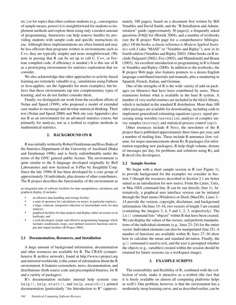
random variable is undefined (Romano and Siegel 1986), thesample mean does not converge to the population parameter.Figure 2 displays the R code to calculate and plot the runningaverage of a sample of Cauchy random variables with center

Figure 2. R code to calculate and display running average.

The American Statistician, November 2004, Vol. 58, No. 4 345

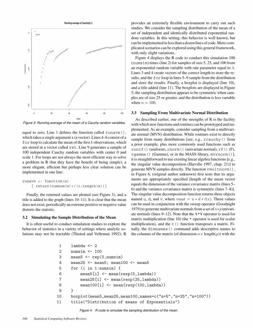
Figure 3. Running average of the mean of a Cauchy random variables.

equal to zero. Line 1 defines the function called runave(),which takes a single argument x (a vector). Lines 4–6 consist of afor loop to calculate the mean of the first k observations, whichare stored in a vector called ret. Line 9 generates a sample of100 independent Cauchy random variables with center 0 andscale 1. For loops are not always the most efficient way to solvea problem in R (but they have the benefit of being simple); amore elegant, efficient but perhaps less clear solution can beimplemented in one line:

runave <- function(x)

{ return(cumsum(x))/(1:length(x))}

Finally, the returned values are plotted (see Figure 3), and atitle is added to the graph (lines 10–11). It is clear that the meandoes not exist; periodically an extreme positive or negative valuedistorts the statistic.

3.2 Simulating the Sample Distribution of the Mean

It is often useful to conduct simulation studies to explore thebehavior of statistics in a variety of settings where analytic so-lutions may not be tractable (Thisted and Velleman 1992); R

provides an extremely flexible environment to carry out suchstudies. We consider the sampling distribution of the mean of aset of independent and identically distributed exponential ran-dom variables. In this setting, this behavior is well known, butcan be implemented in less than a dozen lines of code. More com-plicated scenarios can be explored using this general framework,with only slight variations.

Figure 4 displays the R code to conduct this simulation 100(numsim) times (line 2) for samples of size 5, 25, and 100 froman exponential random variable with rate parameter equal to λ.Lines 3 and 4 create vectors of the correct length to store the re-sults, and the for loop in lines 5–9 sample from the distributionand store the results. Finally, a boxplot is displayed (line 10),and a title added (line 11). The boxplots are displayed in Figure5; the sampling distribution appears to be symmetric when sam-ples are of size 25 or greater, and the distribution is less variablewhen n = 100.

3.3 Sampling From Multivariate Normal Distribution

As described earlier, one of the strengths of R is the facilitywith which new functions and routines can be prototyped and im-plemented. As an example, consider sampling from a multivari-ate normal (MVN) distribution. While routines exist to directlysample from many distributions [see, e.g., rcauchy() froma prior example, plus more commonly used functions such asrunif() (uniform), rnorm() (univariate normal), rf() (F),rgamma() (Gamma), or in the MASS library, mvrnorm()],it is straightforward to use existing linear algebra functions [e.g.,the singular value decomposition (Harville 1997, chap. 21)] togenerate MVN samples directly. The function rmultnorm(),in Figure 6, (original author unknown) first tests that its argu-ments are appropriately specified [length of the mean vectorequals the dimension of the variance covariance matrix (lines 5–6) and the variance covariance matrix is symmetric (lines 7–8)].The singular value decomposition function returns three objectsnamed u, d, and v, where vmat = u ∗ d ∗ t(v). These valuescan be used in conjunction with the sweep operator (Goodnight1979) to generate multivariate normals from a set of n∗p univari-ate normals (lines 9–12). Note that the %*% operator is used formatrix multiplication (line 10) (the * operator is used for scalarmultiplication), and the t() function transposes a matrix. Fi-nally, the dimnames() command adds descriptive names tothe columns of the matrix (of dimension n× length(µ)) with the

Figure 4. R code to simulate the sampling distribution of the mean.


Figure 5. Boxplots of the sampling distribution of the mean.

results (line 13). Although this activity might better be suited to astatistical computing rather than mathematical statistics course,it shows off the matrix algebra capabilities of R.

The function is called (on line 16) to generate a set of 100paired binary outcomes with mean 100, variance 14, and covari-ance 11 (which corresponds to a correlation of 11/14 = .79). Thearguments to the matrix() function include a list of values,and an indication of the dimension of the matrix (here it has tworows, and because there are four entries, the number of columnsequals two). The values in the example were chosen to reflect aset of IQ test results with a mean of 100 and standard deviationof 14. Separate vectors x1 and x2 are created from the 100 × 2

matrix norms (lines 17–18) and a scatterplot of the relationshipbetween the two variables is displayed (line 19, see Figure 7).

3.4 Power and Sample Size Calculations (Analytic)

Power and sample size are confusing concepts for studentsat all levels, and hands-on activities can be helpful in demys-tifying their calculation. One approach to power is to deter-mine the precision of an estimate. We consider the width ofa 95% confidence interval for a proportion, which is given by2 ∗ 1.96 ∗ √

p ∗ (1 − p)/n, where p is the true proportion and nis the sample size. Figure 8 displays the R code and output fora program that calculates and displays these widths for a set ofsample sizes ranging from 100 to 1500 (line 1) and proportionsranging from .10 to .50 (line 2). Lines 6–13 display a header forthe output file, including use of the paste command to turn anR object (in this case the date() function) into a string (line8) and the cat command to output a string (line 6). For eachsample size, the for loop on lines 15–23 calculates the widthfor each of the proportions (note that the object called width isa vector with length equal to the length of prop). The functionround() is used to improve the formatting of the results.

We note that R can be used to execute arbitrary functions inthe underlying operating system (similar to the use of date()on line 8) using the system() command. For example, it isstraightforward for R to run other packages [e.g., symbolic math-ematics programs such as Maple or Mathematica (Baglivo 1995)or any other Unix tool] and read output from those packages.

3.5 Power Calculations (Empirical)

While formulas to calculate power analytically exist for manysettings, there are many situations where such formulas may beintractable or otherwise unappealing. The use of R to simulatedata from a posited distribution and empirically calculate powercan more realistically model the study design, and may be quite

Figure 6. R code for function to generate multivariate normal random variables.


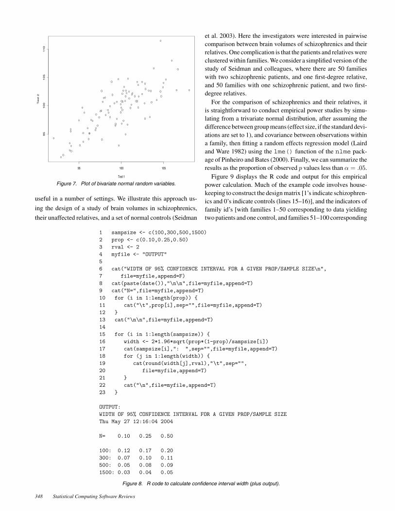
Figure 7. Plot of bivariate normal random variables.

useful in a number of settings. We illustrate this approach us-

ing the design of a study of brain volumes in schizophrenics,

their unaffected relatives, and a set of normal controls (Seidman

et al. 2003). Here the investigators were interested in pairwisecomparison between brain volumes of schizophrenics and theirrelatives. One complication is that the patients and relatives wereclustered within families. We consider a simplified version of thestudy of Seidman and colleagues, where there are 50 familieswith two schizophrenic patients, and one first-degree relative,and 50 families with one schizophrenic patient, and two first-degree relatives.

For the comparison of schizophrenics and their relatives, itis straightforward to conduct empirical power studies by simu-lating from a trivariate normal distribution, after assuming thedifference between group means (effect size, if the standard devi-ations are set to 1), and covariance between observations withina family, then fitting a random effects regression model (Lairdand Ware 1982) using the lme() function of the nlme pack-age of Pinheiro and Bates (2000). Finally, we can summarize theresults as the proportion of observed p values less than α = .05.

Figure 9 displays the R code and output for this empiricalpower calculation. Much of the example code involves house-keeping to construct the design matrix [1’s indicate schizophren-ics and 0’s indicate controls (lines 15–16)], and the indicators offamily id’s [with families 1–50 corresponding to data yieldingtwo patients and one control, and families 51–100 corresponding

Figure 8. R code to calculate confidence interval width (plus output).


Figure 9. R code to estimate power empirically.

to data derived from families with one patient and two controls(lines 17–18)].

Within the loop, thermultnorm() function, defined in Fig-ure 6 is used to generate trivariate normal random variables withthe appropriate means and covariances (lines 24–25). These arestrung together into a single vector y (lines 27–28) with entriesthat correspond to the x and id structures. The lme functionis called specifying a random intercept model (lines 30–31) andthe p value for the appropriate group comparison is saved (line32). If this p value is less than .05 (line 33), then an indica-tor is set to T (True, or 1). After the loops have run, the sumof these indicators (divided by the number of simulations) isused to estimate the power. For these 1,000 simulations, the em-

pirical estimate of power was .89. As a comparison, we alsocalculated the power of a t test comparing two groups assum-ing that all observations were independent. A comparison of150 schizophrenics and 150 relatives with an effect size of .3yields power of .74 (see the power.t.test() function). Inthis setting, since we are interested in a comparison where groupmembership varies within family, accounting for the correlationwithin families yields smaller standard errors. Although analyticformulas to account for correlated outcomes do exist (see, e.g.,Diggle, Heagerty, Liang, and Zeger 2002, secs. 2.4 and 8.5), theytypically require a number of simplifying assumptions, whichmay not always be tenable. Use of R for empirical simulation ofpower is quite flexible.


3.6 Bootstrapping of a Sample Statistic

Bootstrapping is a powerful and versatile approach to param-eter estimation (see Efron and Tibshirani 1993 for a readableintroduction). The observed data are assumed to be a popula-tion, and repeated samples (with replacement) are taken fromthis population. A summary statistic (e.g., the mean) is calcu-lated for each of these samples, and can be used to estimatethe empirical distribution of that statistic. While a number ofadvanced implementations of bootstrapping are available for R(see, e.g., the boot library), it is straightforward to implementthis technique directly.

Figure 10 displays the R code and output for a simple simu-lation to compare 100 ∗ (1−α)% confidence intervals based onthe bootstrap and normal approximations. For this example wetake α = .10. Lines 1–7 set up initialization variables neededfor the simulation, including a call to the qnorm() function todetermine the .95 quantile of a standard normal random variable(1.6449 in this case). For each of the number of simulations, aset of random exponentials is sampled (line 11), normal approx-imation 90% confidence intervals are calculated (line 12), andstored in a matrix of dimension numsim ∗ 2 (line 13). Withinthis loop, another loop runs to generate numboot samples withreplacement from the sample of exponentials, and the α/2 (.05)and 1−α/2 (.95) quantiles are taken from these summary statis-tics (line 20). Finally, an empty plot is made to create appropri-

ate axes (lines 22–23), the matlines() command is used toadd lines (lines 24–25) (a similar command to add points ortext exists), and a legend (line 27) is added. The results from thematplot() function are displayed in Figure 11. In this setting,the performance of the normal approximation and the bootstrapconfidence intervals are quite similar.

3.7 Iteration to Maximize a Likelihood

R is an excellent environment for iterative calculations.Consider, for example, estimation of the unknown parame-ter θ from a set X1, X2, . . . , Xn of independent and identi-cally distributed realizations from a Weibull density f(X|θ) =θλXθ−1 exp (−λXθ), where λ > 0 is known, and θ > 0. Thescore function (derivative of the log-likelihood with respect toθ) is given by:

U(θ|X) =n

θ− λ

n∑

i=1

Xθi ln(Xi) +

n∑

i=1

ln(Xi),

and observed information (negative of the second derivative ofthe log-likelihood):

I(θ|X) =n

θ2 − λ

n∑

i=1

Xθi (ln(Xi))

2.

Figure 10. R code to calculate a bootstrap confidence interval of the mean.


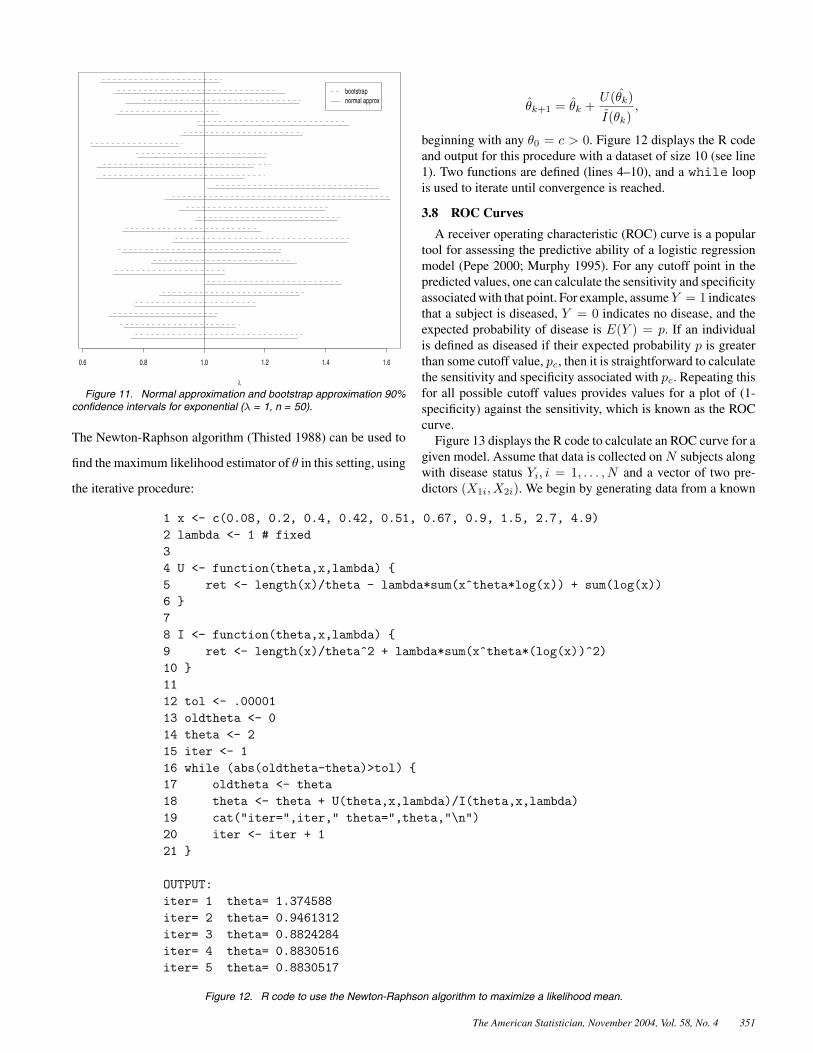
Figure 11. Normal approximation and bootstrap approximation 90%confidence intervals for exponential (λ = 1, n = 50).

The Newton-Raphson algorithm (Thisted 1988) can be used to

find the maximum likelihood estimator of θ in this setting, using

the iterative procedure:

θk+1 = θk +U(θk)I(θk)

,

beginning with any θ0 = c > 0. Figure 12 displays the R codeand output for this procedure with a dataset of size 10 (see line1). Two functions are defined (lines 4–10), and a while loopis used to iterate until convergence is reached.

3.8 ROC Curves

A receiver operating characteristic (ROC) curve is a populartool for assessing the predictive ability of a logistic regressionmodel (Pepe 2000; Murphy 1995). For any cutoff point in thepredicted values, one can calculate the sensitivity and specificityassociated with that point. For example, assume Y = 1 indicatesthat a subject is diseased, Y = 0 indicates no disease, and theexpected probability of disease is E(Y ) = p. If an individualis defined as diseased if their expected probability p is greaterthan some cutoff value, pc, then it is straightforward to calculatethe sensitivity and specificity associated with pc. Repeating thisfor all possible cutoff values provides values for a plot of (1-specificity) against the sensitivity, which is known as the ROCcurve.

Figure 13 displays the R code to calculate an ROC curve for agiven model. Assume that data is collected on N subjects alongwith disease status Yi, i = 1, . . . , N and a vector of two pre-dictors (X1i, X2i). We begin by generating data from a known

Figure 12. R code to use the Newton-Raphson algorithm to maximize a likelihood mean.


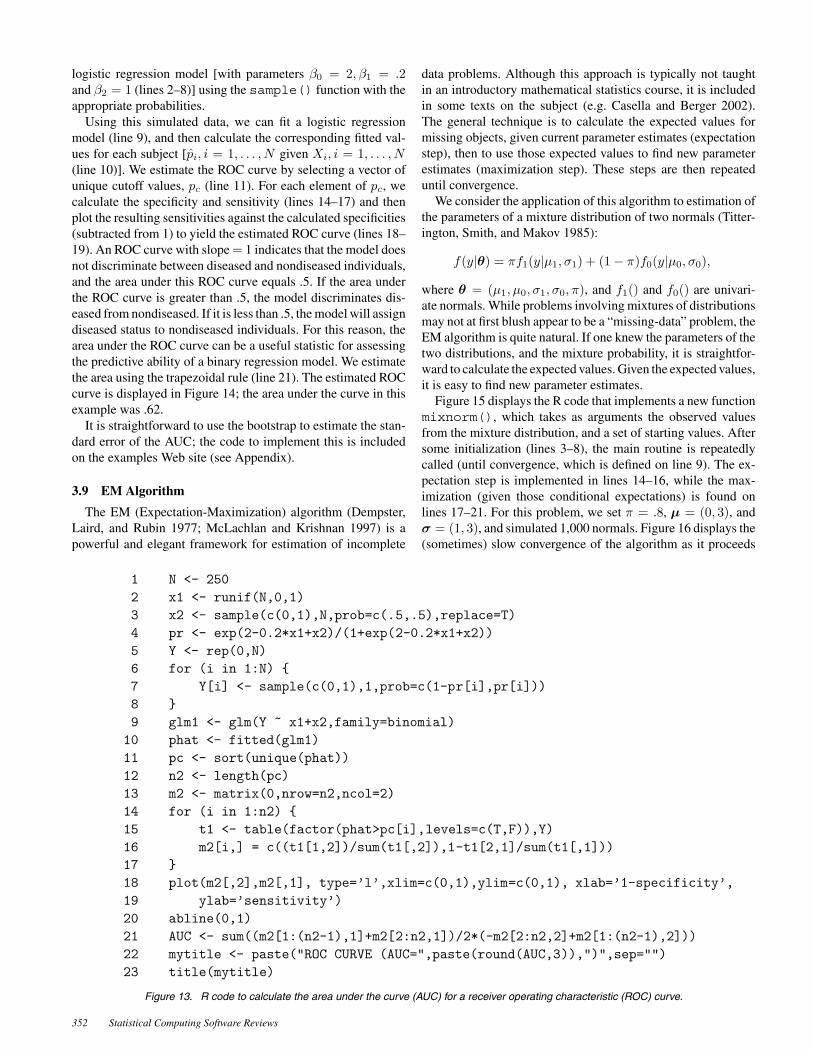
logistic regression model [with parameters β0 = 2, β1 = .2and β2 = 1 (lines 2–8)] using the sample() function with theappropriate probabilities.

Using this simulated data, we can fit a logistic regressionmodel (line 9), and then calculate the corresponding fitted val-ues for each subject [pi, i = 1, . . . , N given Xi, i = 1, . . . , N(line 10)]. We estimate the ROC curve by selecting a vector ofunique cutoff values, pc (line 11). For each element of pc, wecalculate the specificity and sensitivity (lines 14–17) and thenplot the resulting sensitivities against the calculated specificities(subtracted from 1) to yield the estimated ROC curve (lines 18–19). An ROC curve with slope = 1 indicates that the model doesnot discriminate between diseased and nondiseased individuals,and the area under this ROC curve equals .5. If the area underthe ROC curve is greater than .5, the model discriminates dis-eased from nondiseased. If it is less than .5, the model will assigndiseased status to nondiseased individuals. For this reason, thearea under the ROC curve can be a useful statistic for assessingthe predictive ability of a binary regression model. We estimatethe area using the trapezoidal rule (line 21). The estimated ROCcurve is displayed in Figure 14; the area under the curve in thisexample was .62.

It is straightforward to use the bootstrap to estimate the stan-dard error of the AUC; the code to implement this is includedon the examples Web site (see Appendix).

3.9 EM Algorithm

The EM (Expectation-Maximization) algorithm (Dempster,Laird, and Rubin 1977; McLachlan and Krishnan 1997) is apowerful and elegant framework for estimation of incomplete

data problems. Although this approach is typically not taughtin an introductory mathematical statistics course, it is includedin some texts on the subject (e.g. Casella and Berger 2002).The general technique is to calculate the expected values formissing objects, given current parameter estimates (expectationstep), then to use those expected values to find new parameterestimates (maximization step). These steps are then repeateduntil convergence.

We consider the application of this algorithm to estimation ofthe parameters of a mixture distribution of two normals (Titter-ington, Smith, and Makov 1985):

f(y|θ) = πf1(y|µ1, σ1) + (1 − π)f0(y|µ0, σ0),

where θ = (µ1, µ0, σ1, σ0, π), and f1() and f0() are univari-ate normals. While problems involving mixtures of distributionsmay not at first blush appear to be a “missing-data” problem, theEM algorithm is quite natural. If one knew the parameters of thetwo distributions, and the mixture probability, it is straightfor-ward to calculate the expected values. Given the expected values,it is easy to find new parameter estimates.

Figure 15 displays the R code that implements a new functionmixnorm(), which takes as arguments the observed valuesfrom the mixture distribution, and a set of starting values. Aftersome initialization (lines 3–8), the main routine is repeatedlycalled (until convergence, which is defined on line 9). The ex-pectation step is implemented in lines 14–16, while the max-imization (given those conditional expectations) is found onlines 17–21. For this problem, we set π = .8, µ = (0, 3), andσ = (1, 3), and simulated 1,000 normals. Figure 16 displays the(sometimes) slow convergence of the algorithm as it proceeds

Figure 13. R code to calculate the area under the curve (AUC) for a receiver operating characteristic (ROC) curve.


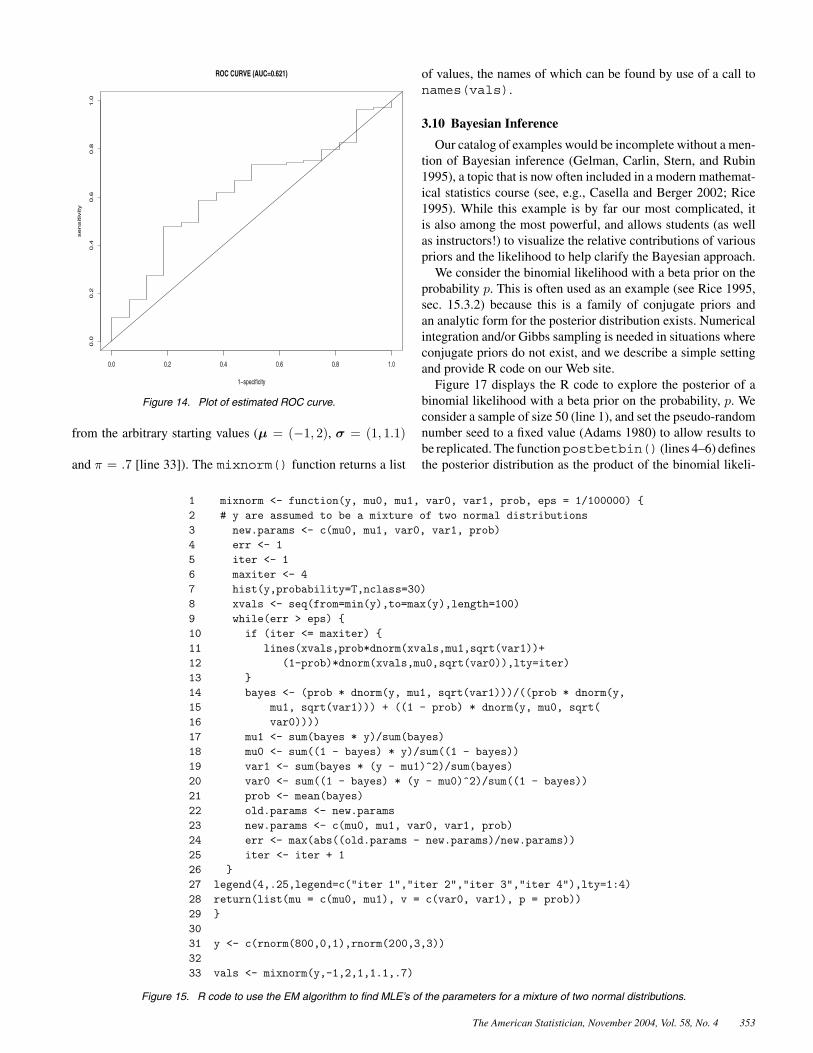
Figure 14. Plot of estimated ROC curve.

from the arbitrary starting values (µ = (−1, 2), σ = (1, 1.1)

and π = .7 [line 33]). The mixnorm() function returns a list

of values, the names of which can be found by use of a call tonames(vals).

3.10 Bayesian Inference

Our catalog of examples would be incomplete without a men-tion of Bayesian inference (Gelman, Carlin, Stern, and Rubin1995), a topic that is now often included in a modern mathemat-ical statistics course (see, e.g., Casella and Berger 2002; Rice1995). While this example is by far our most complicated, itis also among the most powerful, and allows students (as wellas instructors!) to visualize the relative contributions of variouspriors and the likelihood to help clarify the Bayesian approach.

We consider the binomial likelihood with a beta prior on theprobability p. This is often used as an example (see Rice 1995,sec. 15.3.2) because this is a family of conjugate priors andan analytic form for the posterior distribution exists. Numericalintegration and/or Gibbs sampling is needed in situations whereconjugate priors do not exist, and we describe a simple settingand provide R code on our Web site.

Figure 17 displays the R code to explore the posterior of abinomial likelihood with a beta prior on the probability, p. Weconsider a sample of size 50 (line 1), and set the pseudo-randomnumber seed to a fixed value (Adams 1980) to allow results tobe replicated. The functionpostbetbin() (lines 4–6) definesthe posterior distribution as the product of the binomial likeli-

Figure 15. R code to use the EM algorithm to find MLE’s of the parameters for a mixture of two normal distributions.


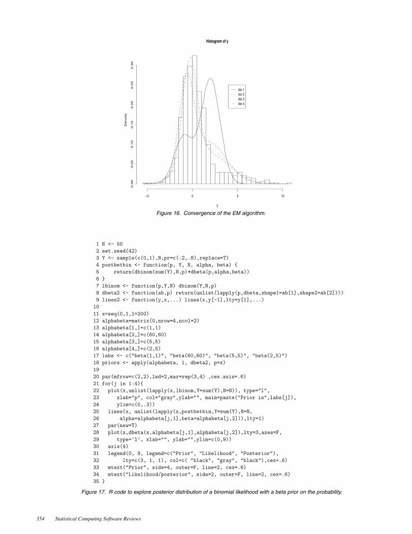
Figure 16. Convergence of the EM algorithm.

Figure 17. R code to explore posterior distribution of a binomial likelihood with a beta prior on the probability.


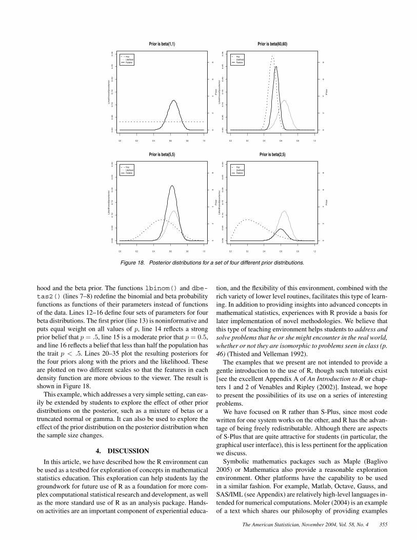
Figure 18. Posterior distributions for a set of four different prior distributions.

hood and the beta prior. The functions lbinom() and dbe-tas2() (lines 7–8) redefine the binomial and beta probabilityfunctions as functions of their parameters instead of functionsof the data. Lines 12–16 define four sets of parameters for fourbeta distributions. The first prior (line 13) is noninformative andputs equal weight on all values of p, line 14 reflects a strongprior belief that p = .5, line 15 is a moderate prior that p = 0.5,and line 16 reflects a belief that less than half the population hasthe trait p < .5. Lines 20–35 plot the resulting posteriors forthe four priors along with the priors and the likelihood. Theseare plotted on two different scales so that the features in eachdensity function are more obvious to the viewer. The result isshown in Figure 18.

This example, which addresses a very simple setting, can eas-ily be extended by students to explore the effect of other priordistributions on the posterior, such as a mixture of betas or atruncated normal or gamma. It can also be used to explore theeffect of the prior distribution on the posterior distribution whenthe sample size changes.

4. DISCUSSION

In this article, we have described how the R environment canbe used as a testbed for exploration of concepts in mathematicalstatistics education. This exploration can help students lay thegroundwork for future use of R as a foundation for more com-plex computational statistical research and development, as wellas the more standard use of R as an analysis package. Hands-on activities are an important component of experiential educa-

tion, and the flexibility of this environment, combined with therich variety of lower level routines, facilitates this type of learn-ing. In addition to providing insights into advanced concepts inmathematical statistics, experiences with R provide a basis forlater implementation of novel methodologies. We believe thatthis type of teaching environment helps students to address andsolve problems that he or she might encounter in the real world,whether or not they are isomorphic to problems seen in class (p.46) (Thisted and Velleman 1992).

The examples that we present are not intended to provide agentle introduction to the use of R, though such tutorials exist[see the excellent Appendix A of An Introduction to R or chap-ters 1 and 2 of Venables and Ripley (2002)]. Instead, we hopeto present the possibilities of its use on a series of interestingproblems.

We have focused on R rather than S-Plus, since most codewritten for one system works on the other, and R has the advan-tage of being freely redistributable. Although there are aspectsof S-Plus that are quite attractive for students (in particular, thegraphical user interface), this is less pertinent for the applicationwe discuss.

Symbolic mathematics packages such as Maple (Baglivo2005) or Mathematica also provide a reasonable explorationenvironment. Other platforms have the capability to be usedin a similar fashion. For example, Matlab, Octave, Gauss, andSAS/IML (see Appendix) are relatively high-level languages in-tended for numerical computations. Moler (2004) is an exampleof a text which shares our philosophy of providing examples


(in his case for a numerical methods course implemented usingMatlab) that students can explore, modify, and extend. Whilethese programs offer a wide variety of routines, they are moregeneral purpose numerical engines than R, and tend to have lesssupport for certain statistical functions.

The flexible programming environment of R is both a plusand a minus as a teaching tool. Students with no prior expe-rience with computer programming may find the environmentuncomfortable at first. The provision of sample code (the me-dian length of our examples was 23 lines) combined with theexistence of built-in functions and routines minimize the pro-gramming requirements and anxiety-level while still providinga rich toolset for experimentation.

APPENDIX

The following list of Web sites, while not comprehensive, isintended to provide a useful starting point for exploring R andrelated tools.

A.1 R AND S-PLUS RESOURCES

http://www.r-project.orgThe home of R: this is the main location for distributions,packages, and documentation.

http://math.smith.edu/∼nhorton/RThis link by the authors provides a repository for sample codeand activities useful in teaching mathematical statistics con-cepts using R.

http://www.insightful.com/productsThis link is the home of S-Plus, a commercial version ofS sold by Insightful Corporation. A number of very usefuladd-on modules provide support for missing data modeling,wavelets, spatial statistics, and design of experiments.

http://www.stat.umn.edu/∼galin/teaching/RstuffThe site provides a general introduction to R. One attractivefeature for those exploring use of R is that it provides a Webinterface to run R on their server.

http://www.stats.ox.ac.uk/pub/MASS4This link contains resource materials (example code, answersto exercises, etc.) for Venables and Ripley’s classic bookModern Applied Statistics with S, now in its fourth edition. Itprovides an introduction to S/R as well as a course in modernstatistical methods.

http://www.stats.ox.ac.uk/pub/MASS3/SprogThe site is a source for background materials for Venables andRipley’s text S Programming which provides a comprehen-sive introduction to programming in S and R. This book isparticularly well-suited for those who like to spelunk in theinnards of complex computing environments.

http://socserv.mcmaster.ca/jfox/Books/CompanionThis link connects to the companion Web site to Fox’s R andS-plus Companion to Applied Regression book.

http://stat-www.berkeley.edu/users/statlabsMaterials related to the book Stat Labs: Mathematical Statis-tics Through Applications (Nolan and Speed 1999), whichteaches the theory of statistics through a collection of ex-tended case studies using R, are found at this link.

A.2 OTHER PACKAGES AND PROCEDURES

http://www.stat.sc.edu/rsrch/gaspThis site is the home of the GASP (globally accessible sta-tistical procedures initiative). It features a number of Javaapplets and Web pages related to data analysis and statisticaleducation.

http://www.keypress.com/fathomFathom is a statistical education tool that allows students tounderstand concepts by dynamic manipulation and simula-tion.

http://www.gnu.orgThis is the home of the GNU (Gnu’s Not Unix) project andthe FSF (Free Software Foundation). The site includes a largenumber of free software packages, including R and Octave,that are available for distribution under the GNU GPL (gen-eral public license). As of July, 2004, 3,316 packages wereindexed on the site.

http://www.mathworks.com/products/matlabMatlab is a commercial high-level technical computing envi-ronment.

http://www.octave.orgThis is the home of the GNU Octave language for numericalcomputations that is mostly compatible with Matlab.

http://www.sas.com/technologies/analytics/statistics/imlThe site provides information on the commercial SAS/IMLinteractive matrix programming environment.

http://www.aptech.comThe official site of the GAUSS system, a data analysis, math-ematical and statistical matrix environment.

REFERENCES

Adams, D. (1980), The Hitchhiker’s Guide to the Galaxy, New York: HarmonyBooks.

American Statistical Association [cited 1 June 2004], Curriculum Guidelines forUndergraduate Programs in Statistical Science [on-line]. Available at http://www.amstat.org/education/index.cfm?fuseaction=Curriculum-Guidelines.

Baglivo, J. (1995), “Computer Algebra Systems: Maple and Mathematica,” TheAmerican Statistician, 49, 86–92.

(2005), Mathematical Laboratories for Mathematical Statistics: Em-phasizing Simulation and Computer Intensive Methods, ASA-SIAM Serieson Statistics and Applied Probability, 14, Alexandria, VA: ASA.

Casella, G., and Berger, R. L. (2002), Statistical Inference (2nd ed.), Belmont,CA: Duxbury.

Cobb, G. (1991), “Teaching Statistics: More Data, Less Lecturing,” UME Trends,3–7.

Dalgaard, P. (2002), Introductory Statistics with R, New York: Springer.Dempster, A. P., Laird, N. M., and Rubin, D. B. (1977), “Maximum Likelihood

From Incomplete Data via the EM Algorithm,” Journal of the Royal StatisticalSociety, Series B, 39, 1–22.

Diggle, P. J., Heagerty, P., Liang, K. Y., and Zeger, S. L. (2002), Analysis ofLongitudinal Data (2nd ed.), Oxford, UK: Clarendon Press.

Eddy, W. F., Jones, A. C., Kass, R. E., and Schervish, M. J. (1987), “Graduate


Education in Computational Statistics,” The American Statistician, 41, 60–64.Efron, B., and Tibshirani, R. J. (1993), An Introduction to the Bootstrap, New

York: Chapman and Hall.Fox, J. (2002), An R and S-Plus Companion to Applied Regression, Thousand

Oaks, CA: Sage Publications.Gelman, A., Carlin, J. B., Stem, H. S., and Rubin, D. B. (1995), Bayesian Data

Analysis, New York: Chapman and Hall.Gentle, J. E. (2004), “Courses in Statistical Computing and Computational

Statistics,” The American Statistician, 58, 2–5.Goodnight, J. H. (1979), “A Tutorial on the SWEEP Operator,” The American

Statistician, 33, 149–158.Harville, D. (1997), Matrix Algebra From a Statistician’s Perspective, New York:

Springer.Hornik, K. [cited 2 June 2004], “The R FAQ” [on-line]. Available at http://www.

ci.tuwien.ac.at/∼hornik/R/.Ihaka, R., and Gentleman, R. (1996), “R: A Language for Data Analysis and

Graphics,” Journal of Computational and Graphical Statistics, 5, 299–314.Laird, N. M., and Ware, J. H. (1982), “Random-Effects Models for Longitudinal

Data,” Biometrics, 38, 963–974.Lange, K. (2004), “Computational Statistics and Optimization Theory at

UCLA,” The American Statistician, 58, 9–11.Maindonald, J., and Braun, J. (2003), Data Analysis and Graphics using R: An

Example-Based Approach, New York: Cambridge University Press.McLachlan, G. J., and Krishnan, T. (1997), The EM Algorithm and Extensions,

New York: Wiley-Interscience.Moler, C. B. (2004), Numerical Computing with Matlab, Philadelphia, PA:

SIAM.Monahan, J. (2004), “Teaching Statistical Computing at North Carolina State

University,” The American Statistician, 58, 6–8.Moore, T. L. (2000), Teaching Statistics: Resources for Undergraduate Instruc-

tors (MAA Notes #52), Washington,DC, and Alexandria, VA: MathematicalAssociation of America and the American Statistical Association.

Murphy, J. M. (1995), “Diagnostic Schedules and Rating Scales in Adult Psy-chiatry,” in Textbook of Psychiatric Epidemiology, New York: Wiley, pp. 253–271.

Nolan, D., and Speed, T. P. (1999), “Teaching Statistics Theory Through Appli-cations,” The American Statistician, 53, 370–375.

(2000), Stat Labs: Mathematical Statistics Through Applications, NewYork: Springer.

Pepe, M. S. (2000), “Receiver Operating Characteristic Methodology,” Journalof the American Statistical Association, 95, 308–311.

Pinheiro, J. C., and Bates, D. M. (2000), Mixed-Effects Models in S and S-PLUS,New York: Springer-Verlag.

R Project [cited 2 June 2004], “What is R?” Available at http://www.r-project.org/about.html/.

Rice, J. A. (1995), Mathematical Statistics and Data Analysis, Belmont, CA:Duxbury.

Romano, J. P., and Siegel, A. F. (1986), Counterexamples in Probability andStatistics, Belmont, CA: Duxbury.

Seidman, L. J., Pantelis, C., Keshavan, M. S., Faraone, S. V., Goldstein, J. M.,Horton, N. J., Makris, N., Falkai, P., Caviness, V. S., and Tsuang, M. T.(2003), “A Review and New Report of Medial Temporal Lobe Dysfunction asa Vulnerability Indicator for Schizophrenia: A Magnetic Resonance ImagingMorphometric Family Study of the Parahippocampal Gyrus,” SchizophreniaBulletin, 29, 803–830.

Thisted, R. A. (1988), Elements of Statistical Computing, New York: Chapmanand Hall.

Thisted, R. A., and Velleman, P. F. (1992), Computers and Modern Statis-tics, MAA Notes number 21, Washington, DC: Mathematical Associationof America, pp. 41–53.

Titterington, D. M., Smith, A. F. M., and Makov, U. E. (1985), Statistical Analysisof Finite Mixture Distributions, New York: Wiley.

Venables, W. N., and Ripley, B. D. (2000), S Programming, New York: Springer.(2002), Modern Applied Statistics With S (4th ed.), New York: Springer.


use of r as a toolbox for mathematical statistics explorationww2.amstat.org/misc/useofr.pdf · use...

Documents