mathematical statistics
DESCRIPTION
数理统计-国人编TRANSCRIPT

Springer Texts in Statistics
Advisors:George Casella Stephen Fienberg Ingram Olkin
SpringerNew YorkBerlinHeidelbergBarcelonaHong KongLondonMilanParisSingaporeTokyo
Springer Texts in Statistics
Alfred: Elements of Statistics for the Life and Social SciencesBerger: An Introduction to Probability and Stochastic ProcessesBlom: Probability and Statistics: Theory and ApplicationsBrockwell and Davis: An Introduction to Times Series and ForecastingChow and Teicher: Probability Theory: Independence, Interchangeability,
Martingales, Third EditionChristensen: Plane Answers to Complex Questions: The Theory of Linear
Models, Second EditionChristensen: Linear Models for Multivariate, Time Series, and Spatial DataChristensen: Log-Linear Models and Logistic Regression, Second EditionCreighton: A First Course in Probability Models and Statistical InferenceDean and Voss: Design and Analysis of Experimentsdu Toit, Steyn, and Stumpf: Graphical Exploratory Data AnalysisEdwards: Introduction to Graphical ModellingFinkelstein and Levin: Statistics for LawyersFlury: A First Course in Multivariate StatisticsJobson: Applied Multivariate Data Analysis, Volume I: Regression and
Experimental DesignJobson: Applied Multivariate Data Analysis, Volume II: Categorical and
Multivariate MethodsKalbfleisch: Probability and Statistical Inference, Volume I: Probability,
Second EditionKalbfleisch: Probability and Statistical Inference, Volume II: Statistical
Inference, Second EditionKarr: ProbabilityKeyfitz: Applied Mathematical Demography, Second EditionKiefer: Introduction to Statistical InferenceKokoska and Nevison: Statistical Tables and FormulaeLehmann: Elements of Large-Sample TheoryLehmann: Testing Statistical Hypotheses, Second EditionLehmann and Casella: Theory of Point Estimation, Second EditionLindman: Analysis of Variance in Experimental DesignLindsey: Applying Generalized Linear ModelsMadansky: Prescriptions for Working StatisticiansMcPherson: Statistics in Scientific Investigation: Its Basis, Application, and
InterpretationMueller: Basic Principles of Structural Equation ModelingNguyen and Rogers: Fundamentals of Mathematical Statistics: Volume I:
Probability for StatisticsNguyen and Rogers: Fundamentals of Mathematical Statistics: Volume II:
Statistical Inference
(Continued after index)

Jun Shao
Mathematical Statistics
Springer
Jun ShaoDepartment of StatisticsUniversity of Wisconsin, MadisonMadison, WI 53706-1685USA
Editorial Board
George Casella Stephen Fienberg Ingram OlkinBiometrics Unit Department of Statistics Department of StatisticsCornell University Carnegie Mellon University Stanford UniversityIthaca, NY 14853-7801 Pittsburgh, PA 15213-3890 Stanford, CA 94305USA USA USA
Library of Congress Cataloging-in-Publication DataShao, Jun.
Mathematical statistics / Jun Shao.p. cm. — (Springer texts in statistics)
Includes bibliographical references and indexes.ISBN 0-387-98674-X (alk. paper)I. Mathematical statistics. I. Title. II. Series.
QA276.S458 1998519.5—<Jdc21 98-45794
© 1999 Springer-Verlag New York, Inc.AH rights reserved. This work may not be translated or copied in whole or in part without thewritten permission of the publisher (Springer-Verlag New York, Inc., 175 Fifth Avenue, New York,NY 10010, USA), except for brief excerpts in connection with reviews or scholarly analysis. Usein connection with any form of information storage and retrieval, electronic adaptation, computersoftware, or by similar or dissimilar methodology now known or hereafter developed is forbidden.The use of general descriptive names, trade names, trademarks, etc., in this publication, even if theformer are not especially identified, is not to be taken as a sign that such names, as understood bythe Trade Marks and Merchandise Marks Act, may accordingly be used freely by anyone.
ISBN 0-387-98674-X Springer-Verlag New York Berlin Heidelberg SPIN 10699982

To Guang, Jason, and Annie
Preface
This book is intended for a course entitled Mathematical Statistics offeredat the Department of Statistics, University of Wisconsin-Madison. Thiscourse, taught in a mathematically rigorous fashion, covers essential ma-terials in statistical theory that a first or second year graduate studenttypically needs to learn as preparation for work on a Ph.D. degree in statis-tics. The course is designed for two 15-week semesters, with three lecturehours and two discussion hours in each week. Students in this course areassumed to have a good knowledge of advanced calculus. A course in realanalysis or measure theory prior to this course is often recommended.
Chapter 1 provides a quick overview of important concepts and resultsin measure-theoretic probability theory that are used as tools in the rest ofthe book. Chapter 2 introduces some fundamental concepts in statistics,including statistical models, the principle of sufficiency in data reduction,and two statistical approaches adopted throughout the book: statisticaldecision theory and statistical inference. Each of Chapters 3 through 7provides a detailed study of an important topic in statistical decision the-ory and inference; Chapter 3 introduces the theory of unbiased estimation;Chapter 4 studies theory and methods in point estimation under paramet-ric models; Chapter 5 covers point estimation in nonparametric settings;Chapter 6 focuses on hypothesis testing; and Chapter 7 discusses inter-val estimation and confidence sets. The classical frequentist approach isadopted in this book, although the Bayesian approach is also introduced(§2.3.2, §4.1, §6.4.4, and §7.1.3). Asymptotic (large sample) theory, a cru-cial part of statistical inference, is studied throughout the book, rather thanin a separate chapter.
About 85% of the book covers classical results in statistical theory thatare typically found in textbooks of a similar level. These materials are in theStatistics Department’s Ph.D. qualifying examination syllabus. This partof the book is influenced by several standard textbooks, such as Casella andBerger (1990), Ferguson (1967), Lehmann (1983, 1986), and Rohatgi (1976).The other 15% of the book covers some topics in modern statistical theory
vii

viii Preface
that have been developed in recent years, including robustness of the leastsquares estimators, Markov chain Monte Carlo, generalized linear models,quasi-likelihoods, empirical likelihoods, statistical functionals, generalizedestimation equations, the jackknife, and the bootstrap.
In addition to the presentation of fruitful ideas and results, this bookemphasizes the use of important tools in establishing theoretical results.Thus, most proofs of theorems, propositions, and lemmas are providedor left as exercises. Some proofs of theorems are omitted (especially inChapter 1), because the proofs are lengthy or beyond the scope of thebook (references are always provided). Each chapter contains a number ofexamples. Part of them are designed as materials covered in the discussionsection of this course, which is typically taught by a teaching assistant (asenior graduate student). The exercises in each chapter form an importantpart of the book. They provide not only practice problems for students,but also many additional results as complementary materials to the maintext.
Appendices A and B provide lists of frequently used abbreviations andnotation, respectively. Definitions, examples, theorems, propositions, corol-laries, and lemmas are numbered according to chapters, and their pagenumbers can be found in the subject index.
The book is essentially based on (1) my class notes taken in 1983-84when I was a student in this course, (2) the notes I used when I was ateaching assistant for this course in 1984-85, and (3) the lecture notes Iprepared during 1997-98 as the instructor of this course. I would like toexpress my thanks to Dennis Cox, who taught this course when I was astudent and a teaching assistant, and undoubtfully has influence on myteaching style and textbook for this course. I am also very grateful tostudents in my class who provided helpful comments; to Mr. Yonghee Lee,who helped me to prepare all the figures in this book; to Springer-VerlagProduction and Copy Editors who helped to improve the presentation; andto my family members who provided support during the writing of thisbook.
Madison, Wisconsin Jun ShaoJanuary 1999
Contents
Preface vii
Chapter 1. Probability Theory 1
1.1 Probability Spaces and Random Elements . . . . . . . . . . . 11.1.1 σ-fields and measures . . . . . . . . . . . . . . . . . . 11.1.2 Measurable functions and distributions . . . . . . . . 6
1.2 Integration and Differentiation . . . . . . . . . . . . . . . . . 91.2.1 Integration . . . . . . . . . . . . . . . . . . . . . . . . 91.2.2 Radon-Nikodym derivative . . . . . . . . . . . . . . . 14
1.3 Distributions and Their Characteristics . . . . . . . . . . . . 171.3.1 Useful probability densities . . . . . . . . . . . . . . . 171.3.2 Moments and generating functions . . . . . . . . . . . 25
1.4 Conditional Expectations . . . . . . . . . . . . . . . . . . . . 301.4.1 Conditional expectations . . . . . . . . . . . . . . . . 301.4.2 Independence . . . . . . . . . . . . . . . . . . . . . . 341.4.3 Conditional distributions . . . . . . . . . . . . . . . . 36
1.5 Asymptotic Theorems . . . . . . . . . . . . . . . . . . . . . . 381.5.1 Convergence modes and stochastic orders . . . . . . . 381.5.2 Convergence of transformations . . . . . . . . . . . . 421.5.3 The law of large numbers . . . . . . . . . . . . . . . . 451.5.4 The central limit theorem . . . . . . . . . . . . . . . . 47
1.6 Exercises . . . . . . . . . . . . . . . . . . . . . . . . . . . . . 49
Chapter 2. Fundamentals of Statistics 61
2.1 Populations, Samples, and Models . . . . . . . . . . . . . . . 612.1.1 Populations and samples . . . . . . . . . . . . . . . . 61
ix
x Contents
2.1.2 Parametric and nonparametric models . . . . . . . . . 642.1.3 Exponential and location-scale families . . . . . . . . 66
2.2 Statistics and Sufficiency . . . . . . . . . . . . . . . . . . . . 702.2.1 Statistics and their distributions . . . . . . . . . . . . 702.2.2 Sufficiency and minimal sufficiency . . . . . . . . . . 732.2.3 Complete statistics . . . . . . . . . . . . . . . . . . . 79
2.3 Statistical Decision Theory . . . . . . . . . . . . . . . . . . . 832.3.1 Decision rules, loss functions, and risks . . . . . . . . 832.3.2 Admissibility and optimality . . . . . . . . . . . . . . 86
2.4 Statistical Inference . . . . . . . . . . . . . . . . . . . . . . . 922.4.1 Point estimators . . . . . . . . . . . . . . . . . . . . . 922.4.2 Hypothesis tests . . . . . . . . . . . . . . . . . . . . . 952.4.3 Confidence sets . . . . . . . . . . . . . . . . . . . . . 99
2.5 Asymptotic Criteria and Inference . . . . . . . . . . . . . . . 1012.5.1 Consistency . . . . . . . . . . . . . . . . . . . . . . . 1022.5.2 Asymptotic bias, variance, and mse . . . . . . . . . . 1052.5.3 Asymptotic inference . . . . . . . . . . . . . . . . . . 109
2.6 Exercises . . . . . . . . . . . . . . . . . . . . . . . . . . . . . 112
Chapter 3. Unbiased Estimation 127
3.1 The UMVUE . . . . . . . . . . . . . . . . . . . . . . . . . . . 1273.1.1 Sufficient and complete statistics . . . . . . . . . . . . 1283.1.2 A necessary and sufficient condition . . . . . . . . . . 1323.1.3 Information inequality . . . . . . . . . . . . . . . . . . 1353.1.4 Asymptotic properties of UMVUE’s . . . . . . . . . . 138
3.2 U-Statistics . . . . . . . . . . . . . . . . . . . . . . . . . . . . 1403.2.1 Some examples . . . . . . . . . . . . . . . . . . . . . . 1403.2.2 Variances of U-statistics . . . . . . . . . . . . . . . . . 1423.2.3 The projection method . . . . . . . . . . . . . . . . . 144
3.3 The LSE in Linear Models . . . . . . . . . . . . . . . . . . . 1483.3.1 The LSE and estimability . . . . . . . . . . . . . . . . 1483.3.2 The UMVUE and BLUE . . . . . . . . . . . . . . . . 1523.3.3 Robustness of LSE’s . . . . . . . . . . . . . . . . . . . 1553.3.4 Asymptotic properties of LSE’s . . . . . . . . . . . . 159
3.4 Unbiased Estimators in Survey Problems . . . . . . . . . . . 161
Contents xi
3.4.1 UMVUE’s of population totals . . . . . . . . . . . . . 1613.4.2 Horvitz-Thompson estimators . . . . . . . . . . . . . 165
3.5 Asymptotically Unbiased Estimators . . . . . . . . . . . . . . 1703.5.1 Functions of unbiased estimators . . . . . . . . . . . . 1703.5.2 The method of moments . . . . . . . . . . . . . . . . 1733.5.3 V-statistics . . . . . . . . . . . . . . . . . . . . . . . . 1763.5.4 The weighted LSE . . . . . . . . . . . . . . . . . . . . 179
3.6 Exercises . . . . . . . . . . . . . . . . . . . . . . . . . . . . . 182
Chapter 4. Estimation in Parametric Models 1934.1 Bayes Decisions and Estimators . . . . . . . . . . . . . . . . 193
4.1.1 Bayes actions . . . . . . . . . . . . . . . . . . . . . . . 1934.1.2 Empirical and hierarchical Bayes methods . . . . . . 1984.1.3 Bayes rules and estimators . . . . . . . . . . . . . . . 2014.1.4 Markov chain Monte Carlo . . . . . . . . . . . . . . . 207
4.2 Invariance . . . . . . . . . . . . . . . . . . . . . . . . . . . . . 2134.2.1 One-parameter location families . . . . . . . . . . . . 2134.2.2 One-parameter scale families . . . . . . . . . . . . . . 2174.2.3 General location-scale families . . . . . . . . . . . . . 219
4.3 Minimaxity and Admissibility . . . . . . . . . . . . . . . . . 2234.3.1 Estimators with constant risks . . . . . . . . . . . . . 2234.3.2 Results in one-parameter exponential families . . . . 2274.3.3 Simultaneous estimation and shrinkage estimators . . 229
4.4 The Method of Maximum Likelihood . . . . . . . . . . . . . 2354.4.1 The likelihood function and MLE’s . . . . . . . . . . 2354.4.2 MLE’s in generalized linear models . . . . . . . . . . 2414.4.3 Quasi-likelihoods and conditional likelihoods . . . . . 245
4.5 Asymptotically Efficient Estimation . . . . . . . . . . . . . . 2484.5.1 Asymptotic optimality . . . . . . . . . . . . . . . . . 2484.5.2 Asymptotic efficiency of MLE’s and RLE’s . . . . . . 2524.5.3 Other asymptotically efficient estimators . . . . . . . 257
4.6 Exercises . . . . . . . . . . . . . . . . . . . . . . . . . . . . . 261
Chapter 5. Estimation in Nonparametric Models 2775.1 Distribution Estimators . . . . . . . . . . . . . . . . . . . . . 277
5.1.1 Empirical c.d.f.’s in i.i.d. cases . . . . . . . . . . . . . 278
xii Contents
5.1.2 Empirical likelihoods . . . . . . . . . . . . . . . . . . 2815.1.3 Density estimation . . . . . . . . . . . . . . . . . . . . 288
5.2 Statistical Functionals . . . . . . . . . . . . . . . . . . . . . . 2915.2.1 Differentiability and asymptotic normality . . . . . . 2915.2.2 L-, M-, R-estimators and rank statistics . . . . . . . . 296
5.3 Linear Functions of Order Statistics . . . . . . . . . . . . . . 3045.3.1 Sample quantiles . . . . . . . . . . . . . . . . . . . . . 3045.3.2 Robustness and efficiency . . . . . . . . . . . . . . . . 3085.3.3 L-estimators in linear models . . . . . . . . . . . . . . 311
5.4 Generalized Estimating Equations . . . . . . . . . . . . . . . 3125.4.1 The GEE method and its relationship with others . . 3135.4.2 Consistency of GEE estimators . . . . . . . . . . . . . 3175.4.3 Asymptotic normality of GEE estimators . . . . . . . 321
5.5 Variance Estimation . . . . . . . . . . . . . . . . . . . . . . . 3255.5.1 The substitution method . . . . . . . . . . . . . . . . 3265.5.2 The jackknife . . . . . . . . . . . . . . . . . . . . . . . 3295.5.3 The bootstrap . . . . . . . . . . . . . . . . . . . . . . 334
5.6 Exercises . . . . . . . . . . . . . . . . . . . . . . . . . . . . . 337
Chapter 6. Hypothesis Tests 345
6.1 UMP Tests . . . . . . . . . . . . . . . . . . . . . . . . . . . . 3456.1.1 The Neyman-Pearson lemma . . . . . . . . . . . . . . 3466.1.2 Monotone likelihood ratio . . . . . . . . . . . . . . . . 3496.1.3 UMP tests for two-sided hypotheses . . . . . . . . . . 353
6.2 UMP Unbiased Tests . . . . . . . . . . . . . . . . . . . . . . 3566.2.1 Unbiasedness and similarity . . . . . . . . . . . . . . 3566.2.2 UMPU tests in exponential families . . . . . . . . . . 3586.2.3 UMPU tests in normal families . . . . . . . . . . . . . 362
6.3 UMP Invariant Tests . . . . . . . . . . . . . . . . . . . . . . 3696.3.1 Invariance and UMPI tests . . . . . . . . . . . . . . . 3696.3.2 UMPI tests in normal linear models . . . . . . . . . . 374
6.4 Tests in Parametric Models . . . . . . . . . . . . . . . . . . . 3806.4.1 Likelihood ratio tests . . . . . . . . . . . . . . . . . . 3806.4.2 Asymptotic tests based on likelihoods . . . . . . . . . 3836.4.3 χ2-tests . . . . . . . . . . . . . . . . . . . . . . . . . . 387
Contents xiii
6.4.4 Bayes tests . . . . . . . . . . . . . . . . . . . . . . . . 392
6.5 Tests in Nonparametric Models . . . . . . . . . . . . . . . . . 394
6.5.1 Sign, permutation, and rank tests . . . . . . . . . . . 394
6.5.2 Kolmogorov-Smirnov and Cramer-von Mises tests . . 398
6.5.3 Empirical likelihood ratio tests . . . . . . . . . . . . . 401
6.5.4 Asymptotic tests . . . . . . . . . . . . . . . . . . . . . 404
6.6 Exercises . . . . . . . . . . . . . . . . . . . . . . . . . . . . . 406
Chapter 7. Confidence Sets 421
7.1 Construction of Confidence Sets . . . . . . . . . . . . . . . . 421
7.1.1 Pivotal quantities . . . . . . . . . . . . . . . . . . . . 421
7.1.2 Inverting acceptance regions of tests . . . . . . . . . . 427
7.1.3 The Bayesian approach . . . . . . . . . . . . . . . . . 430
7.1.4 Prediction sets . . . . . . . . . . . . . . . . . . . . . . 432
7.2 Properties of Confidence Sets . . . . . . . . . . . . . . . . . . 434
7.2.1 Lengths of confidence intervals . . . . . . . . . . . . . 434
7.2.2 UMA and UMAU confidence sets . . . . . . . . . . . 438
7.2.3 Randomized confidence sets . . . . . . . . . . . . . . 441
7.2.4 Invariant confidence sets . . . . . . . . . . . . . . . . 443
7.3 Asymptotic Confidence Sets . . . . . . . . . . . . . . . . . . 445
7.3.1 Asymptotically pivotal quantities . . . . . . . . . . . 445
7.3.2 Confidence sets based on likelihoods . . . . . . . . . . 447
7.3.3 Results for quantiles . . . . . . . . . . . . . . . . . . . 451
7.4 Bootstrap Confidence Sets . . . . . . . . . . . . . . . . . . . 453
7.4.1 Construction of bootstrap confidence intervals . . . . 453
7.4.2 Asymptotic correctness and accuracy . . . . . . . . . 457
7.4.3 High-order accurate bootstrap confidence sets . . . . 463
7.5 Simultaneous Confidence Intervals . . . . . . . . . . . . . . . 467
7.5.1 Bonferroni’s method . . . . . . . . . . . . . . . . . . . 468
7.5.2 Scheffe’s method in linear models . . . . . . . . . . . 469
7.5.3 Tukey’s method in one-way ANOVA models . . . . . 471
7.5.4 Confidence bands for c.d.f.’s . . . . . . . . . . . . . . 473
7.6 Exercises . . . . . . . . . . . . . . . . . . . . . . . . . . . . . 475

xiv Contents
Appendix A. Abbreviations 489
Appendix B. Notation 491
References 493
Author Index 505
Subject Index 509

Chapter 1
Probability Theory
Mathematical statistics relies on probability theory, which in turn is basedon measure theory. The present chapter provides some principal conceptsand notational conventions of probability theory, and some important re-sults that are essential tools used in this book. A more complete account ofprobability theory can be found in many standard textbooks, for example,Billingsley (1986) and Chung (1974). The reader is assumed to be familiarwith set operations and set functions (mappings) in advanced calculus.
1.1 Probability Spaces and Random Elements
In an elementary probability course, one defines a random experiment to bean experiment for which the outcome of the experiment cannot be predictedwith certainty, and the probability of A (a collection of possible outcomes)to be the fraction of times that the outcome of the random experiment re-sults in A in a large number of trials of the random experiment. A rigorousand logically consistent definition of probability was given by A. N. Kol-mogorov in his measure-theoretic fundamental development of probabilitytheory in 1933.
1.1.1 σ-fields and measures
Let Ω be a set of elements of interest. For example, Ω can be a set ofnumbers, a subinterval of the real line, or all possible outcomes of a randomexperiment. In probability theory, Ω is often called the outcome space,whereas in statistical theory, Ω is called the sample space. This is becausein probability and statistics, Ω is usually the set of all possible outcomes ofa random experiment under study.
1
2 1. Probability Theory
A measure is a natural mathematical extension of the length, area, orvolume of subsets in one-, two-, or three-dimensional Euclidean space. Ina given sample space Ω, a measure is a set function defined for certainsubsets of Ω. It will be necessary for this collection of subsets to satisfycertain properties, which are given in the following definition.
Definition 1.1. Let F be a collection of subsets of a sample space Ω. F iscalled a σ-field (or σ-algebra) if and only if it has the following properties.(i) The empty set ∅ ∈ F .(ii) If A ∈ F , then the complement Ac ∈ F .(iii) If Ai ∈ F , i = 1, 2, ..., then their union ∪Ai ∈ F .
A pair (Ω,F) consisting of a set Ω and a σ-field F of subsets of Ω iscalled a measurable space. The elements of F are called measurable sets inmeasure theory or events in probability and statistics.
Since ∅c = Ω, it follows from (i) and (ii) in Definition 1.1 that Ω ∈ Fif F is a σ-field on Ω. Also, it follows from (ii) and (iii) that if Ai ∈ F ,i = 1, 2, ..., and F is a σ-field, then the intersection ∩Ai ∈ F . This can beshown using DeMorgan’s law: (∩Ai)
c = ∪Aci .
For any given Ω, there are two trivial σ-fields. The first one is thecollection containing exactly two elements, ∅ and Ω. This is the smallestpossible σ-field on Ω. The second one is the collection of all subsets of Ω,which is called the power set and is the largest σ-field on Ω.
Let us now consider some nontrivial σ-fields. Let A be a nonemptyproper subset of Ω (A ⊂ Ω, A = Ω). Then (verify)
∅, A,Ac,Ω (1.1)
is a σ-field. In fact, this is the smallest σ-field containing A in the sense thatif F is any σ-field containing A, then the σ-field in (1.1) is a subcollectionof F . In general, the smallest σ-field containing C, a collection of subsets ofΩ, is denoted by σ(C) and is called the σ-field generated by C. Hence, theσ-field in (1.1) is σ(A). Note that σ(A,Ac), σ(A,Ω), and σ(A, ∅)are all the same as σ(A). Of course, if C itself is a σ-field, then σ(C) = C.
On the real line R, there is a special σ-field that will be used almostexclusively. Let C be the collection of all finite open intervals on R. ThenB = σ(C) is called the Borel σ-field. The elements of B are called Borelsets. The Borel σ-field Bk on the k-dimensional Euclidean space Rk canbe similarly defined. It can be shown that all intervals (finite or infinite),open sets, and closed sets are Borel sets. To illustrate, we now show thaton the real line, B = σ(O), where O is the collection of all open sets.Typically, one needs to show that σ(C) ⊂ σ(O) and σ(O) ⊂ σ(C). Since anopen interval is an open set, C ⊂ O and, hence, σ(C) ⊂ σ(O) (see Exercise3 in §1.6). Let U be an open set. Then U can be expressed as a union
1.1. Probability Spaces and Random Elements 3
of a sequence of finite open intervals (see Royden (1968, p.39)). Hence,U ∈ σ(C) (Definition 1.1(iii)) and O ⊂ σ(C). By the definition of σ(O),σ(O) ⊂ σ(C). This completes the proof.
Let C ⊂ Rk be a Borel set and let BC = C ∩ B : B ∈ Bk. Then(C,BC) is a measurable space and BC is called the Borel σ-field on C.
Now we can introduce the notion of a measure.
Definition 1.2. Let (Ω,F) be a measurable space. A set function ν definedon F is called a measure if and only if it has the following properties.(i) 0 ≤ ν(A) ≤ ∞ for any A ∈ F .(ii) ν(∅) = 0.(iii) If Ai ∈ F , i = 1, 2, ..., and Ai’s are disjoint, i.e., Ai ∩ Aj = ∅ for anyi = j, then
ν
( ∞⋃i=1
Ai
)=
∞∑i=1
ν(Ai).
The triple (Ω,F , ν) is called a measure space. If ν(Ω) = 1, then ν iscalled a probability measure and we usually denote it by P instead of ν, inwhich case (Ω,F , P ) is called a probability space.
Although measure is an extension of length, area, or volume, some-times it can be quite abstract. For example, the following set function is ameasure:
ν(A) =
∞ A ∈ F , A = ∅0 A = ∅. (1.2)
Since a measure can take ∞ as its value, we must know how to do arithmeticwith ∞. In this book, it suffices to know that (1) for any x ∈ R, ∞+x = ∞,x∞ = ∞ if x > 0, x∞ = −∞ if x < 0, and 0∞ = 0; (2) ∞+∞ = ∞; and(3) ∞∞ = ∞. However, ∞−∞ or ∞/∞ is not defined.
The following examples provide two very important measures in proba-bility and statistics.
Example 1.1 (Counting measure). Let Ω be a sample space, F the collec-tion of all subsets, and ν(A) the number of elements in A ∈ F (ν(A) = ∞if A contains infinitely many elements). Then ν is a measure on F and iscalled the counting measure.
Example 1.2 (Lebesgue measure). There is a unique measure m on (R,B)that satisfies
m([a, b]) = b− a (1.3)
for every finite interval [a, b], −∞ < a ≤ b < ∞. This is called the Lebesguemeasure. If we restrict m to the measurable space ([0, 1],B[0,1]), then m isa probability measure.
4 1. Probability Theory
If Ω is countable in the sense that there is a one-to-one correspondencebetween Ω and the set of all integers, then one can usually consider thetrivial σ-field that contains all subsets of Ω and a measure that assigns avalue to every subset of Ω. When Ω is uncountable (e.g., Ω = R or [0, 1]),it is not possible to define a reasonable measure for every subset of Ω; forexample, it is not possible to find a measure on all subsets of R and stillsatisfy property (1.3). This is why it is necessary to introduce σ-fields thatare smaller than the power set.
The following result provides some basic properties of measures. When-ever we consider ν(A), it is implicitly assumed that A ∈ F .
Proposition 1.1. Let (Ω,F , ν) be a measure space.(i) (Monotonicity). If A ⊂ B, then ν(A) ≤ ν(B).(ii) (Subadditivity). For any sequence A1, A2, ...,
ν
( ∞⋃i=1
Ai
)≤
∞∑i=1
ν(Ai).
(iii) (Continuity). If A1 ⊂ A2 ⊂ A3 ⊂ · · · (or A1 ⊃ A2 ⊃ A3 ⊃ · · · andν(A1) < ∞), then
ν(
limn→∞
An
)= lim
n→∞ν (An) ,
where
limn→∞
An =∞⋃i=1
Ai
(or =
∞⋂i=1
Ai
).
Proof. We prove (i) only. The proofs of (ii) and (iii) are left as exercises.Since A ⊂ B, B = A ∪ (Ac ∩ B) and A and Ac ∩ B are disjoint. ByDefinition 1.2(iii), ν(B) = ν(A)+ ν(Ac∩B), which is no smaller than ν(A)since ν(Ac ∩B) ≥ 0 by Definition 1.2(i).
There is a one-to-one correspondence between the set of all probabilitymeasures on (R,B) and a set of functions on R. Let P be a probabilitymeasure. The cumulative distribution function (c.d.f.) of P is defined to be
F (x) = P ((−∞, x]) , x ∈ R. (1.4)
Proposition 1.2. (i) Let F be a c.d.f. on R. Then(a) F (−∞) = limx→−∞ F (x) = 0;(b) F (∞) = limx→∞ F (x) = 1;(c) F is nondecreasing, i.e., F (x) ≤ F (y) if x ≤ y;(d) F is right continuous, i.e., limy→x,y>x F (y) = F (x).
(ii) Suppose that a real-valued function F on R satisfies (a)-(d) in part (i).Then F is the c.d.f. of a unique probability measure on (R,B).
1.1. Probability Spaces and Random Elements 5
The Cartesian product of any k sets A1, ..., Ak (which may be subsetsof different sample spaces) is defined as the set of all (a1, ..., ak), ai ∈ Ai,and is denoted by A1 × · · · ×Ak. Let (Ωi,Fi, νi), i = 1, ..., k, be k measurespaces. We now introduce a convenient way of constructing a σ-field and ameasure on the product space Ω1 × · · · × Ωk.
First, note that F1 × · · · × Fk is not necessarily a σ-field. We definethe σ-field σ(F1 × · · · × Fk) as the product σ-field on Ω1 × · · · × Ωk. Asan example, consider (Ωi,Fi) = (R,B) for all i. Then the product space isRk and it can be shown that the product σ-field is the same as the Borelσ-field on Rk, which is the σ-field generated by O, all open sets in Rk.
In Example 1.2, the usual length of an interval [a, b] ⊂ R is the same asthe Lebesgue measure of [a, b]. Consider a rectangle [a1, b1]× [a2, b2] ⊂ R2.The usual area of [a1, b1] × [a2, b2] is
(b1 − a1)(b2 − a2) = m([a1, b1])m([a2, b2]), (1.5)
i.e., the product of the Lebesgue measures of two intervals [a1, b1] and[a2, b2]. Note that [a1, b1] × [a2, b2] is a measurable set by the definitionof the product σ-field. Is m([a1, b1])m([a2, b2]) the same as the value ofa measure defined on the product σ-field? To answer this, we need thefollowing technical definition. A measure ν on (Ω,F) is said to be σ-finiteif there exists a sequence A1, A2, ... such that ∪Ai = Ω and ν(Ai) < ∞for all i. Any finite measure (such as a probability measure) is clearly σ-finite. The Lebesgue measure in Example 1.2 is σ-finite, since R = ∪An
with An = (−n, n), n = 1, 2, .... The counting measure in Example 1.1 is σ-finite if and only if Ω is countable. The measure defined by (1.2), however,is not σ-finite.
Proposition 1.3 (Product measure theorem). Let (Ωi,Fi, νi), i = 1, ..., k,be measure spaces and νi be σ-finite measures. Then there exists a uniqueσ-finite measure on the product σ-field σ(F1 ×· · ·×Fk), called the productmeasure and denoted by ν1 × · · · × νk, such that
ν1 × · · · × νk(A1 × · · · ×Ak) = ν1(A1) · · · νk(Ak)
for all Ai ∈ Fi, i = 1, ..., k.
Thus, in R2 there is a unique measure, the product measure m×m, forwhich m × m([a1, b1] × [a2, b2]) is equal to the value given by (1.5). Thismeasure is called the Lebesgue measure on (R2,B2). Similarly, we candefine the Lebesgue measure on (R3,B3), which exactly equals the usualvolume for subsets of the form [a1, b1] × [a2, b2] × [a3, b3].
In general, the product measure space generated by (Ωi,Fi, νi), i =1, ..., k, is denoted by
∏ki=1(Ωi,Fi, νi).
6 1. Probability Theory
The concept of c.d.f. can be extended to Rk. Let P be a probabilitymeasure on (Rk,Bk). The c.d.f. (or joint c.d.f.) of P is defined by
F (x1, ..., xk) = P ((−∞, x1] × · · · × (−∞, xk]) , xi ∈ R. (1.6)
Note that P is not necessarily a product measure. Again, there is a one-to-one correspondence between probability measures and joint c.d.f.’s on Rk.Some properties of a joint c.d.f. are given in Exercise 10 in §1.6.
1.1.2 Measurable functions and distributions
Since Ω can be quite arbitrary, it is often convenient to consider a function(mapping) f from Ω to a simpler space Λ (often Λ = Rk, the k-dimensionalEuclidean space). Let B ⊂ Λ. Then the inverse image of B under f is
f−1(B) = f ∈ B = ω ∈ Ω : f(ω) ∈ B.The inverse function f−1 need not exist for f−1(B) to be defined. Thereader is asked to verify the following properties:
(a) f−1(Bc) = (f−1(B))c for any B ⊂ Λ;(b) f−1(∪Bi) = ∪f−1(Bi) for any Bi ⊂ Λ, i = 1, 2, ....Let C be a collection of subsets of Λ. We define
f−1(C) = f−1(C) : C ∈ C.
Definition 1.3. Let (Ω,F) and (Λ,G) be measurable spaces and f afunction from Ω to Λ. The function f is called a measurable function from(Ω,F) to (Λ,G) if and only if f−1(G) ⊂ F .
If Λ = R and G = B (Borel σ-field), then f is said to be Borel measurableor is called a Borel function.
In probability theory, a measurable function is called a random elementand denoted by one of X, Y , Z,.... If X is measurable from (Ω,F) to(R,B), then it is called a random variable; if X is measurable from (Ω,F)to (Rk,Bk), then it is called a random k-vector (as a notational conventionin this book, any vector is considered to be a row vector). If X1, ..., Xk arerandom variables defined on a common probability space, then the vector(X1, ..., Xk) is a random k-vector.
If f is measurable from (Ω,F) to (Λ,G), then f−1(G) is a sub-σ-field ofF (verify). It is called the σ-field generated by f and is denoted by σ(f).
Now we consider some examples of measurable functions. If F is thecollection of all subsets of Ω, then any function f is measurable. Let A ⊂ Ω.The indicator function for A is defined as
IA(ω) =
1 ω ∈ A
0 ω ∈ A.
1.1. Probability Spaces and Random Elements 7
For any B ⊂ R,
I−1A (B) =
⎧⎪⎪⎨⎪⎪⎩∅ 0 ∈ B, 1 ∈ B
A 0 ∈ B, 1 ∈ B
Ac 0 ∈ B, 1 ∈ B
Ω 0 ∈ B, 1 ∈ B.
Then σ(IA) is the σ-field given in (1.1). If A is a measurable set, then IAis a Borel function.
Note that σ(IA) is a much smaller σ-field than the original σ-field F .This is another reason why we introduce the concept of measurable func-tions and random variables, in addition to the reason that it is easy todeal with numbers. Often the σ-field F (such as the power set) containstoo many subsets and we are only interested in some of them. One canthen define a random variable X with σ(X) containing subsets that are ofinterest. In general, σ(X) is between the trivial σ-field ∅,Ω and F , andcontains more subsets if X is more complicated. For the simplest functionIA, we have shown that σ(IA) contains only four elements.
The class of simple functions is obtained by taking linear combinationsof indicators of measurable sets, i.e.,
ϕ(ω) =k∑
i=1
aiIAi(ω), (1.7)
where A1, ..., Ak are measurable sets on Ω and a1, ..., ak are real numbers.One can show directly that such a function is a Borel function, but itfollows immediately from Proposition 1.4. Let A1, ..., Ak be a partition ofΩ, i.e., Ai’s are disjoint and A1 ∪ · · · ∪ Ak = Ω. Then the simple functionϕ given by (1.7) with distinct ai’s exactly characterizes this partition andσ(ϕ) = σ(A1, ..., Ak).
Proposition 1.4. Let (Ω,F) be a measurable space.(i) If f and g are Borel, then so are fg and af + bg, where a and b are realnumbers; also, f/g is Borel provided g(ω) = 0 for any ω ∈ Ω.(ii) f is Borel if and only if f−1(a,∞) ∈ F for all a ∈ R.(iii) If f1, f2, ... are Borel, then so are supn fn, infn fn, lim supn fn, andlim infn fn. Furthermore, the set
A =ω ∈ Ω : lim
n→∞fn(ω) exists
is an event and the function
h(ω) =
limn→∞ fn(ω) ω ∈ A
f1(ω) ω ∈ A
8 1. Probability Theory
is Borel.(iv) Suppose that f is measurable from (Ω,F) to (Λ,G) and g is measurablefrom (Λ,G) to (∆,H). Then the composite function gf is measurable from(Ω,F) to (∆,H).(v) Let Ω be a Borel set in Rp. If f is a continuous function from Ω to Rq,then f is measurable.
Proposition 1.4 indicates that there are many Borel functions. In fact,it is hard to find a non-Borel function.
Let (Ω,F , ν) be a measure space and f be a measurable function from(Ω,F) to (Λ,G). The induced measure by f , denoted by νf−1, is a measureon G defined as
ν f−1(B) = ν(f ∈ B) = ν(f−1(B)
), B ∈ G. (1.8)
It is usually easier to deal with ν f−1 than to deal with ν since (Λ,G)is usually simpler than (Ω,F). Furthermore, subsets not in σ(f) are notinvolved in the definition of ν f−1. As we discussed earlier, in some caseswe are only interested in subsets in σ(f).
If ν = P is a probability measure and X is a random variable or arandom vector, then P X−1 is called the law or the distribution of X andis denoted by PX . The c.d.f. of PX defined by (1.4) or (1.6) is also calledthe c.d.f. or joint c.d.f. of X and is denoted by FX . On the other hand,for any c.d.f. or joint c.d.f. F , there exists at least one random variableor vector (usually there are many) defined on some probability space forwhich FX = F . The following are some examples of random variables andtheir c.d.f.’s. More examples can be found in §1.3.1.
Example 1.3 (Discrete c.d.f.’s). Let a1 < a2 < · · · be a sequence of realnumbers and let pn, n = 1, 2, ..., be a sequence of positive numbers suchthat
∑∞n=1 pn = 1. Define
F (x) = ∑n
i=1 pi an ≤ x < an+1, n = 1, 2, ...0 −∞ < x < a1.
(1.9)
Then F is a stepwise c.d.f. It has a jump of size pn at each an and is flatbetween an and an+1, n = 1, 2, .... Such a c.d.f. is called a discrete c.d.f.and the corresponding random variable is called a discrete random variable.We can easily obtain a random variable having F in (1.9) as its c.d.f. Forexample, let Ω = a1, a2, ..., F be the collection of all subsets of Ω,
P (A) =∑
i:ai∈A
pi, A ∈ F , (1.10)
and X(ω) = ω. One can show that P is a probability measure and thec.d.f. of X is F in (1.9).
1.2. Integration and Differentiation 9
Example 1.4 (Continuous c.d.f.’s). Opposite to the class of discrete c.d.f.’sis the class of continuous c.d.f.’s. Without the concepts of integration anddifferentiation introduced in the next section, we can only provide a fewexamples of continuous c.d.f.’s. One such example is the uniform c.d.f. onthe interval [a, b] defined as
F (x) =
⎧⎨⎩0 −∞ < x < ax−ab−a a ≤ x < b
1 b ≤ x < ∞.
Another example is the exponential c.d.f. defined as
F (x) =
0 −∞ < x < 01 − e−x/θ 0 ≤ x < ∞,
where θ is a fixed positive constant. Note that both uniform and exponentialc.d.f.’s are continuous functions.
1.2 Integration and Differentiation
Differentiation and integration are two of the main components of calculus.This is also true in measure theory or probability theory, except that inte-gration is introduced first whereas in calculus, differentiation is introducedfirst.
1.2.1 Integration
An important concept needed in probability and statistics is the integrationof Borel functions with respect to (w.r.t.) a measure ν, which is a type of“average”. The definition proceeds in several steps. First, we define theintegral of a nonnegative simple function, i.e., a simple function ϕ given by(1.7) with ai ≥ 0, i = 1, ..., k.
Definition 1.4(a). The integral of a nonnegative simple function ϕ givenby (1.7) w.r.t. ν is defined as∫
ϕdν =k∑
i=1
aiν(Ai). (1.11)
The right-hand side of (1.11) is a weighted average of ai’s with ν(Ai)’sas weights. Since a∞ = ∞ if a > 0 and a∞ = 0 if a = 0, the right-handside of (1.11) is always well defined, although
∫ϕdν = ∞ is possible. Note
10 1. Probability Theory
that different ai’s and Ai’s may produce the same function ϕ; for example,with Ω = R,
2I(0,1)(x) + I[1,2](x) = I(0,2](x) + I(0,1)(x).
However, one can show that different representations of ϕ in (1.7) pro-duce the same value for
∫ϕdν so that the integral of a nonnegative simple
function is well defined.Next, we consider nonnegative Borel function f .
Definition 1.4(b). Let f be a nonnegative Borel function and let Sf bethe collection of all nonnegative simple functions of the form (1.7) satisfyingϕ(ω) ≤ f(ω) for any ω ∈ Ω. The integral of f w.r.t. ν is defined as∫
fdν = sup∫
ϕdν : ϕ ∈ Sf
.
Hence, for any Borel function f ≥ 0, there exists a sequence of simplefunctions ϕ1, ϕ2, ... such that 0 ≤ ϕi ≤ f for all i and limn→∞
∫ϕndν =∫
fdν.Finally, for a Borel function f , we first define the positive part of f by
f+(ω) = maxf(ω), 0
and the negative part of f by
f−(ω) = max−f(ω), 0.
Note that f+ and f− are nonnegative Borel functions, f(ω) = f+(ω) −f−(ω), and |f(ω)| = f+(ω) + f−(ω).
Definition 1.4(c). Let f be a Borel function. We say∫fdν exists if and
only if at least one of∫f+dν and
∫f−dν is finite, in which case∫
fdν =∫
f+dν −∫
f−dν. (1.12)
Let A be a measurable set and IA be its indicator function. The integralof f over A is defined as ∫
A
fdν =∫
IAfdν.
Note that the left-hand side of (1.12) is always well defined, although itcan be ∞ or −∞. When both
∫f+dν and
∫f−dν are finite, we say that f is
1.2. Integration and Differentiation 11
integrable (for a nonnegative Borel function f , f is integrable if∫fdν < ∞).
Note that the existence of∫fdν is different from the integrability of f .
The integral of f may be denoted differently whenever there is a needto indicate the variable(s) to be integrated and the integration domain; forexample,
∫Ω fdν,
∫f(ω)dν,
∫f(ω)dν(ω), or
∫f(ω)ν(dω), and so on. In
probability and statistics,∫XdP is usually written as EX or E(X) and
called the expectation or expected value of X. If F is the c.d.f. of P on(Rk,Bk),
∫f(x)dP is also denoted by
∫f(x)dF (x) or
∫fdF .
Example 1.5. Let Ω be a countable set, F be all subsets of Ω, and ν bethe counting measure given in Example 1.1. For any Borel function f , theintegral of f w.r.t. ν is ∫
fdν =∑ω∈Ω
f(ω). (1.13)
This is obvious if f is a simple function. The proof for general f is left asan exercise.
Example 1.6. If Ω = R and ν is the Lebesgue measure, then the integralof f over an interval [a, b] agrees with the Riemann integral in calculus whenthe latter is well defined, and is usually written as
∫[a,b] f(x)dx =
∫ b
af(x)dx.
However, there are functions for which the Lebesgue integrals are definedbut not the Riemann integrals.
We now introduce some properties of integrals. The proof of the follow-ing result is left to the reader.
Proposition 1.5 (Linearity of integrals). Let (Ω,F , ν) be a measure spaceand f and g be Borel functions.(i) If
∫fdν exists and a ∈ R, then
∫(af)dν exists and is equal to a
∫fdν.
(ii) If both∫fdν and
∫gdν exist and
∫fdν +
∫gdν is well defined, then∫
(f + g)dν exists and is equal to∫fdν +
∫gdν.
If a statement holds for all ω in Ω−N with ν(N ) = 0, then the statementis said to hold a.e. (almost every where) ν (or simply a.e. if the measure νis clear from the context). If ν is a probability measure, then a.e. may bereplaced by a.s. (almost surely).
Proposition 1.6. Let (Ω,F , ν) be a measure space and f and g be Borel.(i) If f ≤ g a.e., then
∫fdν ≤
∫gdν, provided that the integrals exist.
(ii) If f ≥ 0 a.e. and∫fdν = 0, then f = 0 a.e.
Some direct consequences of Proposition 1.6(i) are: |∫fdν| ≤
∫|f |dν;
if f ≥ 0 a.e., then∫fdν ≥ 0; and if f = g a.e., then
∫fdν =
∫gdν.
12 1. Probability Theory
We now prove part (ii) of Proposition 1.6 as an illustration. The prooffor part (i) is left to the reader. Let A = f > 0 and An = f ≥ n−1,n = 1, 2, .... Then An ⊂ A for any n and limn→∞ An = A (why?). ByProposition 1.1(iii), limn→∞ ν(An) = ν(A). Using Proposition 1.5 andpart (i) of Proposition 1.6, we obtain that
n−1ν(An) =∫
n−1IAndν ≤∫
fIAndν ≤∫
fdν = 0
for any n. Hence ν(A) = 0 and f = 0 a.e.It is sometimes required to know whether the following interchange of
two operations is valid:∫limn→∞
fndν = limn→∞
∫fndν, (1.14)
where f1, f2, ... is a sequence of Borel functions. Note that we only requirelimn→∞ fn exists a.e. Also, the limit of a sequence of Borel functions isBorel (Proposition 1.4). The following example shows that (1.14) is notalways true.
Example 1.7. Consider (R,B) and the Lebesgue measure. Define fn(x) =nI[0,n−1](x), n = 1, 2, .... Then limn→∞ fn(x) = 0 for all x but x = 0.Since the Lebesgue measure of a single point set is 0 (see Example 1.2),limn→∞ fn(x) = 0 a.e. and
∫limn→∞ fn(x)dx = 0. On the other hand,∫
fn(x)dx = 1 for any n and, hence, limn→∞∫fn(x)dx = 1.
The following result gives some sufficient conditions under which (1.14)holds.
Theorem 1.1. Let f1, f2, ... be a sequence of Borel functions.(i) (Dominated convergence theorem). If limn→∞ fn = f a.e. and thereexists an integrable function g such that |fn| ≤ g a.e., then (1.14) holds.(ii) (Fatou’s lemma). If fn ≥ 0, then∫
lim infn
fndν ≤ lim infn
∫fndν.
(iii) (Monotone convergence theorem). If 0 ≤ f1 ≤ f2 ≤ · · · and limn→∞ fn= f a.e., then (1.14) holds.
The proof is omitted. However, it can be seen that if f in (iii) is in-tegrable, then part (iii) is a consequence of part (i). The following is anapplication of Theorem 1.1.
Example 1.8 (Interchange of differentiation and integration). Let (Ω,F , ν)be a measure space and for any fixed θ, f(ω, θ) be a Borel function on
1.2. Integration and Differentiation 13
Ω. Suppose that ∂f(ω, θ)/∂θ exists a.e. for θ ∈ (a, b) ⊂ R and that|∂f(ω, θ)/∂θ| ≤ g(ω) a.e., where g is an integrable function on Ω. Then,for each θ ∈ (a, b), ∂f(ω, θ)/∂θ is integrable and
d
dθ
∫f(ω, θ)dν =
∫∂f(ω, θ)
∂θdν.
Theorem 1.2 (Change of variables). Let f be measurable from (Ω,F , ν)to (Λ,G) and g be Borel on (Λ,G). Then∫
Ωg fdν =
∫Λgd(ν f−1), (1.15)
i.e., if either integral exists, then so does the other, and the two are thesame.
The proof is again omitted. Note that integration domains are indicatedon both sides of (1.15). This result extends the change of variable formulafor Riemann integrals, i.e.,
∫g(y)dy =
∫g(f(x))f ′(x)dx, y = f(x).
Result (1.15) is very important in probability and statistics. Let Xbe a random variable on a probability space (Ω,F , P ). If EX =
∫Ω XdP
exists, then usually it is much simpler to compute EX =∫R xdPX , where
PX = P X−1 is the law of X. Let Y be a random vector from Ω to Rk andg be Borel from Rk to R. According to (1.15), Eg(Y ) can be computed as∫Rk g(y)dPY or
∫R xdPg(Y ), depending on which of PY and Pg(Y ) is easier
to handle. As a more specific example, consider k = 2, Y = (X1, X2), andg(Y ) = X1 + X2. Using Proposition 1.5(ii), E(X1 + X2) = EX1 + EX2and, hence,
E(X1 + X2) =∫RxdPX1 +
∫RxdPX2 .
Then we need to handle two integrals involving PX1 and PX2 . On the otherhand,
E(X1 + X2) =∫RxdPX1+X2 ,
which involves one integral w.r.t. PX1+X2 . Unless we have some knowledgeabout the joint c.d.f. of (X1, X2), it is not easy to handle PX1+X2 .
The following theorem states how to evaluate an integral w.r.t. a productmeasure via iterated integration.
Theorem 1.3 (Fubini’s theorem). Let νi be a σ-finite measure on (Ωi,Fi),i = 1, 2, and let f be a Borel function on
∏2i=1(Ωi,Fi) whose integral w.r.t.
ν1 × ν2 exists. Then
g(ω2) =∫
Ω1
f(ω1, ω2)dν1
14 1. Probability Theory
exists a.e. ν2 and defines a Borel function on Ω2 whose integral w.r.t. ν2exists, and∫
Ω1×Ω2
f(ω1, ω2)dν1 × ν2 =∫
Ω2
[∫Ω1
f(ω1, ω2)dν1
]dν2.
This result can be naturally extended to the integral w.r.t. the productmeasure on
∏ki=1(Ωi,Fi) for any finite positive integer k.
Example 1.9. Let Ω1 = Ω2 = 0, 1, 2, ..., and ν1 = ν2 be the countingmeasure (Example 1.1). A function f on Ω1×Ω2 defines a double sequence.If
∫fdν1 × ν2 exists, then∫
fdν1 × ν2 =∞∑i=0
∞∑j=0
f(i, j) =∞∑j=0
∞∑i=0
f(i, j) (1.16)
(by Theorem 1.3 and Example 1.5). Thus, a double series can be summedin either order, if it is well defined.
1.2.2 Radon-Nikodym derivative
Let (Ω,F , ν) be a measure space and f be a nonnegative Borel function.One can show that the set function
λ(A) =∫A
fdν, A ∈ F (1.17)
is a measure on (Ω,F). Note that
ν(A) = 0 implies λ(A) = 0. (1.18)
If (1.18) holds for two measures λ and ν defined on the same measurablespace, then we say λ is absolutely continuous w.r.t. ν, and write λ ν.
Formula (1.17) gives us not only a way of constructing measures, butalso a method of computing measures of measurable sets. Let ν be a well-known measure (such as the Lebesgue measure or the counting measure)and λ a relatively unknown measure. If we can find a function f such that(1.17) holds, then computing λ(A) can be done through integration. Anecessary condition for (1.17) is clearly λ ν. The following result showsthat λ ν is also almost sufficient for (1.17).
Theorem 1.4 (Radon-Nikodym theorem). Let ν and λ be two measureson (Ω,F) and ν be σ-finite. If λ ν, then there exists a nonnegative Borel
1.2. Integration and Differentiation 15
function f on Ω such that (1.17) holds. Furthermore, f is unique a.e. ν,i.e., if λ(A) =
∫Agdν for any A ∈ F , then f = g a.e. ν.
The proof of this theorem is beyond our scope. If (1.17) holds, then thefunction f is called the Radon-Nikodym derivative or density of λ w.r.t. ν,and is denoted by dλ/dν.
A useful consequence of Theorem 1.4 is that if f is Borel on (Ω,F) and∫Afdν = 0 for any A ∈ F , then f = 0 a.e.If
∫fdν = 1 for an f ≥ 0 a.e. ν, then λ given by (1.17) is a probability
measure and f is called its probability density function (p.d.f.) w.r.t. ν. Forany probability measure P on Rk corresponding to a c.d.f. F or a randomvector X, if P has a p.d.f. f w.r.t. a measure ν, then f is also called thep.d.f. of F or X w.r.t. ν.
Example 1.10 (p.d.f. of a discrete c.d.f.). Consider the discrete c.d.f. Fin (1.9) of Example 1.3 with its probability measure given by (1.10). LetΩ = a1, a2, ... and ν be the counting measure on the power set of Ω. ByExample 1.5,
P (A) =∫A
fdν =∑ai∈A
f(ai), A ⊂ Ω, (1.19)
where f(ai) = pi, i = 1, 2, .... That is, f is the p.d.f. of P or F w.r.t. ν.Hence any discrete c.d.f. has a p.d.f. w.r.t. counting measure. A p.d.f. w.r.t.counting measure is called a discrete p.d.f.
Example 1.11. Let F be a c.d.f. Assume that F is differentiable in theusual sense in calculus. Let f be the derivative of F . From calculus,
F (x) =∫ x
−∞f(y)dy, x ∈ R. (1.20)
Let P be the probability measure corresponding to F . It can be shownthat P (A) =
∫Afdm for any A ∈ B, where m is the Lebesgue measure on
R. Hence, f is the p.d.f. of P or F w.r.t. Lebesgue measure. In this case,the Radon-Nikodym derivative is the same as the usual derivative of F incalculus.
A continuous c.d.f. may not have a p.d.f. w.r.t. Lebesgue measure.A necessary and sufficient condition for a c.d.f. F having a p.d.f. w.r.t.Lebesgue measure is that F is absolute continuous in the sense that forany ε > 0, there exists δ > 0 such that for each finite collection of disjointbounded open intervals (ai, bi),
∑(bi−ai) < δ implies
∑[F (bi)−F (ai)] < ε.
Absolute continuity is weaker than differentiability, but is stronger thancontinuity. Thus, any discontinuous c.d.f. (such as a discrete c.d.f.) is notabsolute continuous. Note that every c.d.f. is differentiable a.e. Lebesgue
16 1. Probability Theory
measure (Chung, 1974, Chapter 1). Hence, if f is the p.d.f. of F w.r.t.Lebesgue measure, then f = the usual derivative of F a.e. Lebesgue mea-sure and (1.20) holds. In such a case probabilities can be computed throughintegration. It can be shown that the uniform and exponential c.d.f.’s inExample 1.4 are absolute continuous and their p.d.f.’s are, respectively,
f(x) =
1
b−a a ≤ x < b
0 otherwise
and
f(x) =
0 −∞ < x < 0θ−1e−x/θ 0 ≤ x < ∞.
A p.d.f. w.r.t. Lebesgue measure is called a Lebesgue p.d.f.
More examples of p.d.f.’s are given in §1.3.1.The following result provides some basic properties of Radon-Nikodym
derivatives.
Proposition 1.7 (Calculus with Radon-Nikodym derivatives). Let ν be aσ-finite measure on a measure space (Ω,F). All other measures discussedin (i)-(iii) are defined on (Ω,F).(i) If λ is a measure, λ ν, and f ≥ 0, then∫
fdλ =∫
fdλ
dνdν.
(Notice how the dν’s “cancel” on the right-hand side.)(ii) If λi, i = 1, 2, are measures and λi ν, then λ1 + λ2 ν and
d(λ1 + λ2)dν
=dλ1
dν+
dλ2
dνa.e. ν.
(iii) (Chain rule). If τ is a measure, λ is a σ-finite measure, and τ λ ν,then
dτ
dν=
dτ
dλ
dλ
dνa.e. ν.
In particular, if λ ν and ν λ (in which case λ and ν are equivalent),then
dλ
dν=
(dν
dλ
)−1
a.e. ν or λ.
(iv) Let (Ωi,Fi, νi) be a measure space and νi be σ-finite, i = 1, 2. Let λi
be a measure on (Ωi,Fi) and λi νi, i = 1, 2. Then λ1 × λ2 ν1 × ν2and
d(λ1 × λ2)d(ν1 × ν2)
(ω1, ω2) =dλ1
dν1(ω1)
dλ2
dν2(ω2) a.e. ν1 × ν2.
1.3. Useful Distributions and Their Characteristics 17
1.3 Distributions and Their Characteristics
We now discuss some distributions useful in statistics, and their momentsand generating functions.
1.3.1 Useful probability densities
It is often more convenient to work with p.d.f.’s than to work with c.d.f.’s.We now introduce some p.d.f.’s useful in statistics.
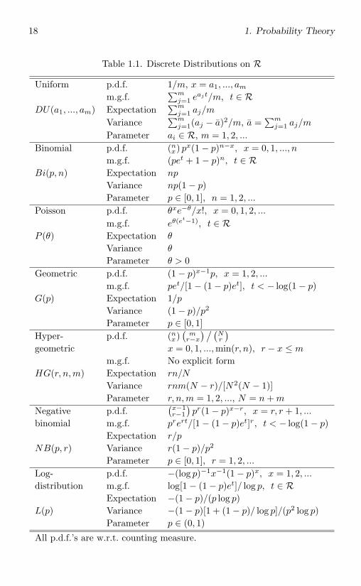
Most discrete p.d.f.’s are w.r.t. counting measure on the space of allnonnegative integers. Table 1.1 lists all discrete p.d.f.’s in elementary prob-ability textbooks. For any discrete p.d.f. f , its c.d.f. F (x) can be obtainedusing (1.19) with A = (∞, x]. Values of F (x) can be obtained from statis-tical tables or software.
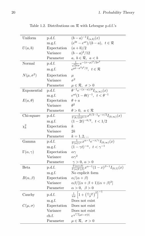
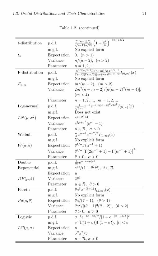
Two Lebesgue p.d.f.’s are introduced in Example 1.11. Some otheruseful Lebesgue p.d.f.’s are listed in Table 1.2. Note that the exponentialp.d.f. in Example 1.11 is a special case of that in Table 1.2 with a = 0. Forany Lebesgue p.d.f., (1.20) gives its c.d.f. A few c.d.f.’s have explicit forms,whereas many others do not and they have to be evaluated numerically orcomputed using tables or software.
There are p.d.f.’s that are neither discrete nor Lebesgue.
Example 1.12. Let X be a random variable on (Ω,F , P ) whose c.d.f. FX
has a Lebesgue p.d.f. fX and FX(c) < 1, where c is a fixed constant. LetY = min(X, c), i.e., Y is the smaller of X and c. Note that Y −1((−∞, x]) =Ω if x ≥ c and Y −1((−∞, x]) = X−1((∞, x]) if x < c. Hence Y is a randomvariable and the c.d.f. of Y is
FY (x) =
1 x ≥ c
FX(x) x < c.
This c.d.f. is discontinuous at c, since F (c) < 1. Thus, it does not have aLebesgue p.d.f. It is not discrete either. Does PY , the probability measurecorresponding to FY , has a p.d.f. w.r.t. some measure? Define a probabilitymeasure on (R,B), called point mass at c, by
δc(A) =
1 c ∈ A
0 c ∈ A,A ∈ B (1.21)
(which is a special case of the discrete uniform distribution in Table 1.1).Then PY m+ δc, where m is the Lebesgue measure, and the p.d.f. of PY
is
dPY
d(m + δc)(x) =
⎧⎨⎩0 x > c
1 − FX(c) x = c
fX(x) x < c.
(1.22)
18 1. Probability Theory
Table 1.1. Discrete Distributions on R
Uniform p.d.f. 1/m, x = a1, ..., amm.g.f.
∑mj=1 e
ajt/m, t ∈ RDU(a1, ..., am) Expectation
∑mj=1 aj/m
Variance∑m
j=1(aj − a)2/m, a =∑m
j=1 aj/m
Parameter ai ∈ R, m = 1, 2, ...Binomial p.d.f. (nx) px(1 − p)n−x, x = 0, 1, ..., n
m.g.f. (pet + 1 − p)n, t ∈ RBi(p, n) Expectation np
Variance np(1 − p)Parameter p ∈ [0, 1], n = 1, 2, ...
Poisson p.d.f. θxe−θ/x!, x = 0, 1, 2, ...m.g.f. eθ(e
t−1), t ∈ RP (θ) Expectation θ
Variance θ
Parameter θ > 0Geometric p.d.f. (1 − p)x−1p, x = 1, 2, ...
m.g.f. pet/[1 − (1 − p)et], t < − log(1 − p)G(p) Expectation 1/p
Variance (1 − p)/p2
Parameter p ∈ [0, 1]Hyper- p.d.f. (nx)
(mr−x
) / (Nr
)geometric x = 0, 1, ...,min(r, n), r − x ≤ m
m.g.f. No explicit formHG(r, n,m) Expectation rn/N
Variance rnm(N − r)/[N2(N − 1)]Parameter r, n,m = 1, 2, ..., N = n + m
Negative p.d.f.(x−1r−1
)pr(1 − p)x−r, x = r, r + 1, ...
binomial m.g.f. prert/[1 − (1 − p)et]r, t < − log(1 − p)Expectation r/p
NB(p, r) Variance r(1 − p)/p2
Parameter p ∈ [0, 1], r = 1, 2, ...Log- p.d.f. −(log p)−1x−1(1 − p)x, x = 1, 2, ...distribution m.g.f. log[1 − (1 − p)et]/ log p, t ∈ R
Expectation −(1 − p)/(p log p)L(p) Variance −(1 − p)[1 + (1 − p)/ log p]/(p2 log p)
Parameter p ∈ (0, 1)
All p.d.f.’s are w.r.t. counting measure.
1.3. Useful Distributions and Their Characteristics 19
The random variable Y in Example 1.12 is a transformation of therandom variable X. Transformations of random variables or vectors arefrequently used in probability and statistics. For a random variable orvector X, f(X) is a random variable or vector as long as f is measurable(Proposition 1.4). How do we find the c.d.f. (or p.d.f.) of f(X) when thec.d.f. (or p.d.f.) of X is known? In many cases, the most effective method isdirect computation. Example 1.12 is one example. The following is anotherone.
Example 1.13. Let X be a random variable with c.d.f. FX and Lebesguep.d.f. fX , and let Y = X2. Note that Y −1((−∞, x]) = ∅ if x < 0 andY −1((−∞, x]) = Y −1([0, x]) = X−1([−√
x,√x ]) if x ≥ 0. Hence
FY (x) = P Y −1((−∞, x])= P X−1([−
√x,
√x ])
= FX(√x) − FX(−
√x)
if x ≥ 0 and FY (x) = 0 if x < 0. Clearly, the Lebesgue p.d.f. of FY is
fY (x) =1
2√x
[fX(√x) + fX(−
√x)]I(0,∞)(x). (1.23)
In particular, if
fX(x) =1√2π
e−x2/2, (1.24)
which is the Lebesgue p.d.f. for the normal distribution N(0, 1) (Table 1.2),then
fY (x) =1√2πx
e−x/2I(0,∞)(x),
which is the Lebesgue p.d.f. for the chi-square distribution χ21 (Table 1.2).
This is actually an important result in statistics.
In some cases one may apply the following general result.
Proposition 1.8. Let X be a random k-vector with a Lebesgue p.d.f. fXand let Y = g(X), where g is a Borel function from (Rk,Bk) to (Rk,Bk).Let A1, ..., Am be disjoint subsets of Rk such that Rk − (A1 ∪ · · · ∪ Am)has Lebesgue measure 0 and g on Aj is one-to-one with a nonvanishingJacobian, i.e., Det(∂g(x)/∂x) = 0 on Aj , j = 1, ...,m, where Det(M) is thedeterminant of a square matrix M . Then Y has the following Lebesguep.d.f.:
fY (x) =m∑j=1
∣∣Det (∂hj(x)/∂x)∣∣ fX (hj(x)) ,
where hj is the inverse function of g on Aj , j = 1, ...,m.
20 1. Probability Theory
Table 1.2. Distributions on R with Lebesgue p.d.f.’s
Uniform p.d.f. (b− a)−1I(a,b)(x)m.g.f. (ebt − eat)/(b− a), t ∈ R
U(a, b) Expectation (a + b)/2Variance (b− a)2/12Parameter a, b ∈ R, a < b
Normal p.d.f. 1√2πσ
e−(x−µ)2/2σ2
m.g.f. eµt−σ2t2/2, t ∈ RN(µ, σ2) Expectation µ
Variance σ2
Parameter µ ∈ R, σ > 0Exponential p.d.f. θ−1e−(x−a)/θI(a,∞)(x)
m.g.f. eat(1 − θt)−1, t < θ−1
E(a, θ) Expectation θ + a
Variance θ2
Parameter θ > 0, a ∈ RChi-square p.d.f. 1
Γ(k/2)2k/2 xk/2−1e−x/2I(0,∞)(x)
m.g.f. (1 − 2t)−k/2, t < 1/2χ2k Expectation k
Variance 2kParameter k = 1, 2, ...
Gamma p.d.f. 1Γ(α)γαx
α−1e−x/γI(0,∞)(x)m.g.f. (1 − γt)−α, t < γ−1
Γ(α, γ) Expectation αγ
Variance αγ2
Parameter γ > 0, α > 0Beta p.d.f. Γ(α+β)
Γ(α)Γ(β)xα−1(1 − x)β−1I(0,1)(x)
m.g.f. No explicit formB(α, β) Expectation α/(α + β)
Variance αβ/[(α + β + 1)(α + β)2]Parameter α > 0, β > 0
Cauchy p.d.f. 1πσ
[1 +
(x−µσ
)2]−1
m.g.f. Does not existC(µ, σ) Expectation Does not exist
Variance Does not existch.f. e
√−1µt−σ|t|
Parameter µ ∈ R, σ > 0
1.3. Useful Distributions and Their Characteristics 21
Table 1.2. (continued)
t-distribution p.d.f. Γ[(n+1)/2]√nπΓ(n/2)
(1 + x2
n
)−(n+1)/2
m.g.f. No explicit formtn Expectation 0, (n > 1)
Variance n/(n− 2), (n > 2)Parameter n = 1, 2, ...
F-distribution p.d.f. nn/2mm/2Γ[(n+m)/2]xn/2−1
Γ(n/2)Γ(m/2)(m+nx)(n+m)/2 I(0,∞)(x)m.g.f. No explicit form
Fn,m Expectation m/(m− 2), (m > 2)Variance 2m2(n + m− 2)/[n(m− 2)2(m− 4)],
(m > 4)Parameter n = 1, 2, ..., m = 1, 2, ...
Log-normal p.d.f. 1√2πσ
x−1e−(log x−µ)2/2σ2I(0,∞)(x)
m.g.f. Does not existLN(µ, σ2) Expectation eµ+σ2/2
Variance e2µ+σ2(eσ
2 − 1)Parameter µ ∈ R, σ > 0
Weibull p.d.f. αθ x
α−1e−xα/θI(0,∞)(x)m.g.f. No explicit form
W (α, θ) Expectation θ1/αΓ(α−1 + 1)Variance θ2/α
[Γ(2α−1 + 1) − Γ(α−1 + 1)
]2Parameter θ > 0, α > 0
Double p.d.f. 12θ e
−|x−µ|/θ
Exponential m.g.f. eµt/(1 + θ2t2), t ∈ RExpectation µ
DE(µ, θ) Variance 2θ2
Parameter µ ∈ R, θ > 0Pareto p.d.f. θaθx−(θ+1)I(a,∞)(x)
m.g.f. No explicit formPa(a, θ) Expectation θa/(θ − 1), (θ > 1)
Variance θa2/[(θ − 1)2(θ − 2)], (θ > 2)Parameter θ > 0, a > 0
Logistic p.d.f. σ−1e−(x−µ)/σ/[1 + e−(x−µ)/σ]2
m.g.f. eµtΓ(1 + σt)Γ(1 − σt), |t| < σ
LG(µ, σ) Expectation µ
Variance σ2π2/3Parameter µ ∈ R, σ > 0
22 1. Probability Theory
One may apply Proposition 1.8 to obtain result (1.23) in Example 1.13,using A1 = (−∞, 0), A2 = (0,∞), and g(x) = x2. Note that h1(x) = −√
x,h2(x) =
√x, and |dhj(x)/dx| = 1/(2
√x).
A p.d.f. corresponding to a joint c.d.f. is called a joint p.d.f. The fol-lowing is an important joint Lebesgue p.d.f. in statistics:
f(x) = (2π)−k/2[Det(Σ)]−1/2e−(x−µ)Σ−1(x−µ)τ/2, x ∈ Rk, (1.25)
where µ ∈ Rk is a vector of parameters, Σ is a positive definite k×k matrixof parameters, and Aτ denotes the transpose of a vector or matrix A. Thep.d.f. in (1.25) and its c.d.f. are called the k-dimensional multivariate normalp.d.f. and c.d.f. and both are denoted by Nk(µ,Σ). The normal distributionN(µ, σ2) in Table 1.2 is a special case of Nk(µ,Σ) with k = 1. The p.d.f. in(1.24) is N(0, 1) and is called the standard normal p.d.f. Sometimes randomvectors having the Nk(µ,Σ) distribution are also denoted by Nk(µ,Σ) forconvenience. Useful properties of multivariate normal distributions can befound in Exercise 51.
Let X be a random k-vector having a c.d.f. FX . Then the ith componentof X is a random variable Xi having the following c.d.f.:
FXi(x) = limxj→∞,j=1,...,i−1,i+1,...,k
FX(x1, ..., xi−1, x, xi+1, ..., xk),
which is called the marginal c.d.f. of Xi. That is, the k marginal c.d.f.’s aredetermined by the joint c.d.f. If FX has a Lebesgue p.d.f. fX , then Xi hasthe following Lebesgue p.d.f.:
fXi(x) =
∫· · ·
∫fX(x1, ..., xi−1, x, xi+1, ..., xk)dx1 · · · dxi−1dxi+1 · · · dxk.
In general, a joint c.d.f. cannot be determined by k marginal c.d.f.’s. Thereis one special but important case in which the joint c.d.f. of a randomk-vector is determined by its k marginal c.d.f.’s, i.e.,
FX(x1, ..., xk) = FX1(x1) · · ·FXk(xk), (x1, ..., xk) ∈ Rk. (1.26)
If (1.26) holds, then random variables X1, ..., Xk are said to be independent.The meaning of independence is further discussed in §1.4.2. If each Xi hasa Lebesgue p.d.f. fXi , then X1, ..., Xk are independent if and only if thejoint p.d.f. of X satisfies
fX(x1, ..., xk) = fX1(x1) · · · fXk(xk), (x1, ..., xk) ∈ Rk. (1.27)
Example 1.14. Let X = (X1, X2) be a random 2-vector having a jointLebesgue p.d.f. fX . Consider first the transformation g(x) = (x1, x1 + x2).Using Proposition 1.8, one can show that the joint p.d.f. of g(X) is
fg(X)(x1, y) = fX(x1, y − x1),
1.3. Useful Distributions and Their Characteristics 23
where y = x1 + x2 (note that the Jacobian equals 1). The marginal p.d.f.of Y = X1 + X2 is then
fY (y) =∫
fX(x1, y − x1)dx1.
In particular, if X1 and X2 are independent, then
fY (y) =∫
fX1(x1)fX2(y − x1)dx1. (1.28)
Next, consider the transformation h(x1, x2) = (x1/x2, x2), assuming thatX2 = 0 a.s. Using Proposition 1.8, one can show that the joint p.d.f. ofh(X) is
fh(X)(z, x2) = |x2|fX(zx2, x2),
where z = x1/x2. The marginal p.d.f. of Z = X1/X2 is
fZ(z) =∫
|x2|fX(zx2, x2)dx2.
In particular, if X1 and X2 are independent, then
fZ(z) =∫
|x2|fX1(zx2)fX2(x2)dx2. (1.29)
A number of results can be derived from (1.28) and (1.29). For example,if X1 and X2 are independent and both have the standard normal p.d.f.given by (1.24), then, by (1.29), the Lebesgue p.d.f. of Z = X1/X2 is
fZ(z) =12π
∫|x2|e−(1+z2)x2
2/2dx2
=1π
∫ ∞
0e−(1+z2)xdx
=1
π(1 + z2),
which is the p.d.f. of the Cauchy distribution C(0, 1) in Table 1.2. Anotherapplication of formula (1.29) leads to the following important result instatistics.
Example 1.15 (t-distribution and F-distribution). Let X1 and X2 beindependent random variables having the chi-square distributions χ2
n1and
χ2n2
(Table 1.2), respectively. By (1.29), the p.d.f. of Z = X1/X2 is
fZ(z) =zn1/2−1I(0,∞)(z)
2(n1+n2)/2Γ(n1/2)Γ(n2/2)
∫ ∞
0x
(n1+n2)/2−12 e−(1+z)x2/2dx2
=Γ[(n1 + n2)/2]Γ(n1/2)Γ(n2/2)
zn1/2−1
(1 + z)(n1+n2)/2I(0,∞)(z),
24 1. Probability Theory
where the last equality follows from the fact that
12(n1+n2)/2Γ[(n1 + n2)/2]
x(n1+n2)/2−12 e−x2/2I(0,∞)(x2)
is the p.d.f. of the chi-square distribution χ2n1+n2
. Using Proposition 1.8,one can show that the p.d.f. of Y = (X1/n1)/(X2/n2) = (n2/n1)Z is thep.d.f. of the F-distribution Fn1,n2 given in Table 1.2.
Let U1 be a random variable having the standard normal distributionN(0, 1) and U2 a random variable having the chi-square distribution χ2
n.Using the same argument, one can show that if U1 and U2 are independent,then the distribution of T = U1/
√U2/n is the t-distribution tn given in
Table 1.2. This result can also be derived using the result given in thisexample as follows. Let X1 = U2
1 and X2 = U2. Then X1 and X2 areindependent (which can be shown directly, but follows immediately fromProposition 1.13 in §1.4.2). By Example 1.13, the distribution of X1 is χ2
1.Then Y = X1/(X2/n) has the F-distribution F1,n and its Lebesgue p.d.f.is
nn/2Γ[(n + 1)/2]x−1/2√nπΓ(n/2)(n + x)(n+1)/2 I(0,∞)(x).
Note that
T = √
Y U1 ≥ 0−√Y U1 < 0.
The result follows from Proposition 1.8 and the fact that
P T−1 ((−∞,−t]) = P T−1 ([t,∞)) , t > 0. (1.30)
If a random variable T satisfies (1.30), then T and its c.d.f. and p.d.f.(if it exists) are said to be symmetric about 0. If T has a Lebesgue p.d.f.fT , then T is symmetric about 0 if and only if fT (x) = fT (−x) for anyx > 0. T and its c.d.f. and p.d.f. are said to be symmetric about a (orsymmetric for simplicity) if and only if T − a is symmetric about 0 for afixed a ∈ R. The c.d.f.’s of t-distributions are symmetric about 0 and thenormal, Cauchy, and double exponential c.d.f.’s are symmetric.
The chi-square, t-, and F-distributions in the previous examples arespecial cases of the following noncentral chi-square, t-, and F-distributions,which are useful in some statistical problems.
Let X1, ..., Xn be independent random variables and Xi = N(µi, σ2),
i = 1, ..., n. The distribution of the random variable Y = (X21 +· · ·+X2
n)/σ2
is called the noncentral chi-square distribution and denoted by χ2n(δ), where
δ = (µ21 + · · · + µ2
n)/σ2 is the noncentrality parameter. It can be shown
1.3. Useful Distributions and Their Characteristics 25
(exercise) that Y has the following Lebesgue p.d.f.:
e−δ/2∞∑j=0
δj
2jj!f2j+n(x), (1.31)
where fk(x) is the Lebesgue p.d.f. of the chi-square distribution χ2k. It is
easy to see that the chi-square distribution χ2k in Table 1.2 is a special case
of the noncentral chi-square distribution χ2k(δ) with δ = 0 and, therefore,
is called a central chi-square distribution.The result for the t-distribution in Example 1.15 can be extended to the
case where U1 has a nonzero expectation (U2 still has the χ2n distribution
and is independent of U1). The distribution of T = U1/√U2/n is called
the noncentral t-distribution and denoted by tn(δ), where δ = µ is thenoncentrality parameter. Using the same argument as that in Example1.15, one can show (exercise) that T has the following Lebesgue p.d.f.:
12(n+1)/2Γ(n/2)
√πn
∫ ∞
0y(n−1)/2e−[(x
√y/n−δ)2+y]/2dy. (1.32)
The t-distribution tn in Example 1.15 is called a central t-distribution, sinceit is a special case of the noncentral t-distribution tn(δ) with δ = 0.
Similarly, the result for the F-distribution in Example 1.15 can be ex-tended to the case where X1 has the noncentral chi-square distributionχ2n1
(δ), X2 has the central chi-square distribution χ2n2
, and X1 and X2are independent. The distribution of Y = (X1/n1)/(X2/n2) is called thenoncentral F-distribution and denoted by Fn1,n2(δ), where δ is the non-centrality parameter. It can be shown (exercise) that Y has the followingLebesgue p.d.f.:
e−δ/2nn1/21 n
n2/22
Γ(n2/2)
∞∑j=0
(δn1x/2)jΓ((n1 + n2)/2 + j)xn1/2−1
j!Γ(n1/2 + j)(n1x + n2)(n1+n2)/2+jI(0,∞)(x).
(1.33)The F-distribution Fn1,n2 in Example 1.15 is called a central F-distribution,since it is a special case of the noncentral F-distribution Fn1,n2(δ) withδ = 0.
1.3.2 Moments and generating functions
We have defined the expectation of a random variable in §1.2.1. It is animportant characteristic of a random variable. In this section we introduceother important moments and two generating functions of a random vector.
Let X be a random variable. If EXk is finite, where k is a positiveinteger, then EXk is called the kth moment of X (or the distribution of
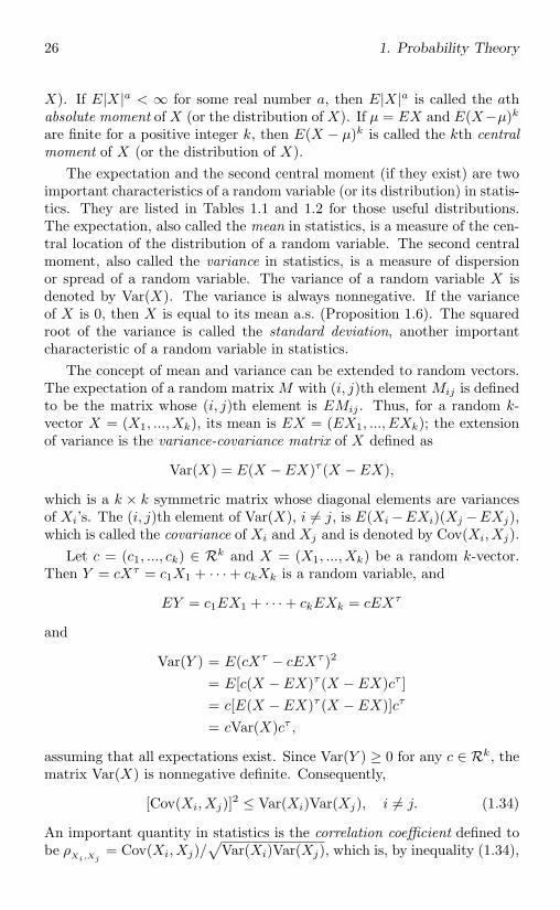
26 1. Probability Theory
X). If E|X|a < ∞ for some real number a, then E|X|a is called the athabsolute moment of X (or the distribution of X). If µ = EX and E(X−µ)k
are finite for a positive integer k, then E(X − µ)k is called the kth centralmoment of X (or the distribution of X).
The expectation and the second central moment (if they exist) are twoimportant characteristics of a random variable (or its distribution) in statis-tics. They are listed in Tables 1.1 and 1.2 for those useful distributions.The expectation, also called the mean in statistics, is a measure of the cen-tral location of the distribution of a random variable. The second centralmoment, also called the variance in statistics, is a measure of dispersionor spread of a random variable. The variance of a random variable X isdenoted by Var(X). The variance is always nonnegative. If the varianceof X is 0, then X is equal to its mean a.s. (Proposition 1.6). The squaredroot of the variance is called the standard deviation, another importantcharacteristic of a random variable in statistics.
The concept of mean and variance can be extended to random vectors.The expectation of a random matrix M with (i, j)th element Mij is definedto be the matrix whose (i, j)th element is EMij . Thus, for a random k-vector X = (X1, ..., Xk), its mean is EX = (EX1, ..., EXk); the extensionof variance is the variance-covariance matrix of X defined as
Var(X) = E(X − EX)τ (X − EX),
which is a k × k symmetric matrix whose diagonal elements are variancesof Xi’s. The (i, j)th element of Var(X), i = j, is E(Xi−EXi)(Xj −EXj),which is called the covariance of Xi and Xj and is denoted by Cov(Xi, Xj).
Let c = (c1, ..., ck) ∈ Rk and X = (X1, ..., Xk) be a random k-vector.Then Y = cXτ = c1X1 + · · · + ckXk is a random variable, and
EY = c1EX1 + · · · + ckEXk = cEXτ
and
Var(Y ) = E(cXτ − cEXτ )2
= E[c(X − EX)τ (X − EX)cτ ]= c[E(X − EX)τ (X − EX)]cτ
= cVar(X)cτ ,
assuming that all expectations exist. Since Var(Y ) ≥ 0 for any c ∈ Rk, thematrix Var(X) is nonnegative definite. Consequently,
[Cov(Xi, Xj)]2 ≤ Var(Xi)Var(Xj), i = j. (1.34)
An important quantity in statistics is the correlation coefficient defined tobe ρ
Xi,Xj= Cov(Xi, Xj)/
√Var(Xi)Var(Xj), which is, by inequality (1.34),
1.3. Useful Distributions and Their Characteristics 27
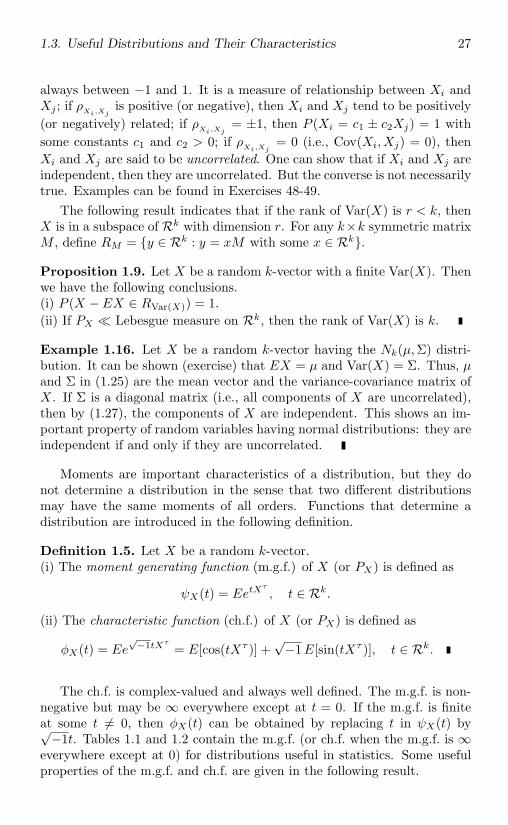
always between −1 and 1. It is a measure of relationship between Xi andXj ; if ρ
Xi,Xjis positive (or negative), then Xi and Xj tend to be positively
(or negatively) related; if ρXi,Xj
= ±1, then P (Xi = c1 ± c2Xj) = 1 withsome constants c1 and c2 > 0; if ρ
Xi,Xj= 0 (i.e., Cov(Xi, Xj) = 0), then
Xi and Xj are said to be uncorrelated. One can show that if Xi and Xj areindependent, then they are uncorrelated. But the converse is not necessarilytrue. Examples can be found in Exercises 48-49.
The following result indicates that if the rank of Var(X) is r < k, thenX is in a subspace of Rk with dimension r. For any k×k symmetric matrixM , define RM = y ∈ Rk : y = xM with some x ∈ Rk.
Proposition 1.9. Let X be a random k-vector with a finite Var(X). Thenwe have the following conclusions.(i) P (X − EX ∈ RVar(X)) = 1.(ii) If PX Lebesgue measure on Rk, then the rank of Var(X) is k.
Example 1.16. Let X be a random k-vector having the Nk(µ,Σ) distri-bution. It can be shown (exercise) that EX = µ and Var(X) = Σ. Thus, µand Σ in (1.25) are the mean vector and the variance-covariance matrix ofX. If Σ is a diagonal matrix (i.e., all components of X are uncorrelated),then by (1.27), the components of X are independent. This shows an im-portant property of random variables having normal distributions: they areindependent if and only if they are uncorrelated.
Moments are important characteristics of a distribution, but they donot determine a distribution in the sense that two different distributionsmay have the same moments of all orders. Functions that determine adistribution are introduced in the following definition.
Definition 1.5. Let X be a random k-vector.(i) The moment generating function (m.g.f.) of X (or PX) is defined as
ψX(t) = EetXτ
, t ∈ Rk.
(ii) The characteristic function (ch.f.) of X (or PX) is defined as
φX(t) = Ee√−1tXτ
= E[cos(tXτ )] +√−1E[sin(tXτ )], t ∈ Rk.
The ch.f. is complex-valued and always well defined. The m.g.f. is non-negative but may be ∞ everywhere except at t = 0. If the m.g.f. is finiteat some t = 0, then φX(t) can be obtained by replacing t in ψX(t) by√−1t. Tables 1.1 and 1.2 contain the m.g.f. (or ch.f. when the m.g.f. is ∞
everywhere except at 0) for distributions useful in statistics. Some usefulproperties of the m.g.f. and ch.f. are given in the following result.
28 1. Probability Theory
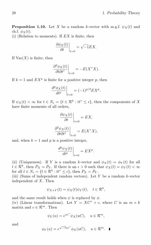
Proposition 1.10. Let X be a random k-vector with m.g.f. ψX(t) andch.f. φX(t).(i) (Relation to moments). If EX is finite, then
∂φX(t)∂t
∣∣∣∣t=0
=√−1EX.
If Var(X) is finite, then
∂2φX(t)∂t∂tτ
∣∣∣∣t=0
= −E(XτX).
If k = 1 and EXp is finite for a positive integer p, then
dpφX(t)dtp
∣∣∣∣t=0
= (−1)p/2EXp.
If ψX(t) < ∞ for t ∈ Nε = t ∈ Rk : ttτ ≤ ε, then the components of Xhave finite moments of all orders,
∂ψX(t)∂t
∣∣∣∣t=0
= EX,
∂2ψX(t)∂t∂tτ
∣∣∣∣t=0
= E(XτX),
and, when k = 1 and p is a positive integer,
dpψX(t)dtp
∣∣∣∣t=0
= EXp.
(ii) (Uniqueness). If Y is a random k-vector and φX(t) = φY (t) for allt ∈ Rk, then PX = PY . If there is an ε > 0 such that ψX(t) = ψY (t) < ∞for all t ∈ Nε = t ∈ Rk : ttτ ≤ ε, then PX = PY .(iii) (Sums of independent random vectors). Let Y be a random k-vectorindependent of X. Then
ψX+Y (t) = ψX(t)ψY (t), t ∈ Rk,
and the same result holds when ψ is replaced by φ.(iv) (Linear transformations). Let Y = XCτ + c, where C is an m × kmatrix and c ∈ Rm. Then
ψY (u) = eucτ
ψX(uC), u ∈ Rm,
andφY (u) = e
√−1ucτφX(uC), u ∈ Rm.
1.3. Useful Distributions and Their Characteristics 29
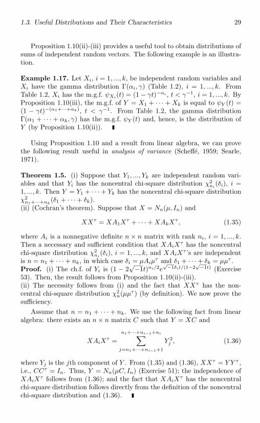
Proposition 1.10(ii)-(iii) provides a useful tool to obtain distributions ofsums of independent random vectors. The following example is an illustra-tion.
Example 1.17. Let Xi, i = 1, ..., k, be independent random variables andXi have the gamma distribution Γ(αi, γ) (Table 1.2), i = 1, ..., k. FromTable 1.2, Xi has the m.g.f. ψXi
(t) = (1 − γt)−αi , t < γ−1, i = 1, ..., k. ByProposition 1.10(iii), the m.g.f. of Y = X1 + · · · + Xk is equal to ψY (t) =(1 − γt)−(α1+···+αk), t < γ−1. From Table 1.2, the gamma distributionΓ(α1 + · · · + αk, γ) has the m.g.f. ψY (t) and, hence, is the distribution ofY (by Proposition 1.10(ii)).
Using Proposition 1.10 and a result from linear algebra, we can provethe following result useful in analysis of variance (Scheffe, 1959; Searle,1971).
Theorem 1.5. (i) Suppose that Y1, ..., Yk are independent random vari-ables and that Yi has the noncentral chi-square distribution χ2
ni(δi), i =
1, ..., k. Then Y = Y1 + · · · + Yk has the noncentral chi-square distributionχ2n1+···+nk
(δ1 + · · · + δk).(ii) (Cochran’s theorem). Suppose that X = Nn(µ, In) and
XXτ = XA1Xτ + · · · + XAkX
τ , (1.35)
where Ai is a nonnegative definite n × n matrix with rank ni, i = 1, ..., k.Then a necessary and sufficient condition that XAiX
τ has the noncentralchi-square distribution χ2
ni(δi), i = 1, ..., k, and XAiX
τ ’s are independentis n = n1 + · · · + nk, in which case δi = µAiµ
τ and δ1 + · · · + δk = µµτ .Proof. (i) The ch.f. of Yi is (1 − 2
√−1t)ni/2e
√−1δit/(1−2
√−1t) (Exercise
53). Then, the result follows from Proposition 1.10(ii)-(iii).(ii) The necessity follows from (i) and the fact that XXτ has the non-central chi-square distribution χ2
n(µµτ ) (by definition). We now prove thesufficiency.
Assume that n = n1 + · · · + nk. We use the following fact from linearalgebra: there exists an n× n matrix C such that Y = XC and
XAiXτ =
n1+···+ni−1+ni∑j=n1+···+ni−1+1
Y 2j , (1.36)
where Yj is the jth component of Y . From (1.35) and (1.36), XXτ = Y Y τ ,i.e., CCτ = In. Thus, Y = Nn(µC, In) (Exercise 51); the independence ofXAiX
τ follows from (1.36); and the fact that XAiXτ has the noncentral
chi-square distribution follows directly from the definition of the noncentralchi-square distribution and (1.36).
30 1. Probability Theory
1.4 Conditional Expectations
In elementary probability the conditional probability of an event B givenan event A is defined as P (B|A) = P (A∩B)/P (A), provided that P (A) >0. In probability and statistics, however, we sometimes need a notion of“conditional probability” even for A’s with P (A) = 0; for example, A =Y = c, where Y is a random variable and c ∈ R. General definitionsof conditional probability, expectation, and distribution are introduced inthis section, and they are shown to agree with those defined in elementaryprobability in special cases.
1.4.1 Conditional expectations
Definition 1.6. Let X be an integrable random variable on (Ω,F , P ).(i) Let A be a sub-σ-field of F . The conditional expectation of X givenA, denoted by E(X|A), is the a.s.-unique random variable satisfying thefollowing two conditions:
(a) E(X|A) is measurable from (Ω,A) to (R,B);(b)
∫AE(X|A)dP =
∫AXdP for any A ∈ A.
(ii) Let B ∈ F . The conditional probability of B given A is defined to beP (B|A) = E(IB |A).(iii) Let Y be measurable from (Ω,F , P ) to (Λ,G). The conditional expec-tation of X given Y is defined to be E(X|Y ) = E[X|σ(Y )].
Essentially, the σ-field σ(Y ) contains “the information in Y ”. Hence,E(X|Y ) is the “expectation” of X given the information provided by σ(Y ).The following useful result shows that there is a Borel function h definedon the range of Y such that E(X|Y ) = h Y .
Theorem 1.6. Let Y be measurable from (Ω,F) to (Λ,G) and Z a functionfrom (Ω,F) to Rk. Then Z is measurable from (Ω, σ(Y )) to (Rk,Bk) ifand only if there is a measurable function h from (Λ,G) to (Rk,Bk) suchthat Z = h Y .
The function h in E(X|Y ) = h Y is a Borel function on (Λ,G). Lety ∈ Λ. Then we define
E(X|Y = y) = h(y)
to be the conditional expectation of X given Y = y. Note that h(y) is afunction on Λ, whereas h Y is a function on Ω.
Example 1.18. Let X be an integrable random variable on (Ω,F , P ),A1, A2, ... be disjoint events on (Ω,F , P ) such that ∪Ai = Ω and P (Ai) > 0
1.4. Conditional Expectations and Distributions 31
for all i, and let a1, a2, ... be distinct real numbers. Define Y = a1IA1 +a2IA2 + · · ·. We now show that
E(X|Y ) =∞∑i=1
∫Ai
XdP
P (Ai)IAi . (1.37)
We need to verify (a) and (b) in Definition 1.6 with A = σ(Y ). Sinceσ(Y ) = σ(A1, A2, ...), it is clear that the function on the right-hand sideof (1.37) is measurable on (Ω, σ(Y )). For any B ∈ B, Y −1(B) = ∪i:ai∈BAi.Using properties of integrals, we obtain that∫
Y −1(B)XdP =
∑i:ai∈B
∫Ai
XdP
=∞∑i=1
∫Ai
XdP
P (Ai)P
(Ai ∩ Y −1(B)
)=
∫Y −1(B)
[ ∞∑i=1
∫Ai
XdP
P (Ai)IAi
]dP.
This verifies (b) and thus (1.37) holds.Let A ∈ F and X = IA. Then
P (A|Y ) = E(X|Y ) =∞∑i=1
P (A ∩Ai)P (Ai)
IAi .
Note that Y = ai = ω ∈ Ω : Y (ω) = ai = Ai. If ω ∈ Ai,
P (A|Y )(ω) =P (A ∩Ai)P (Ai)
= P (A|Ai) = P (A|Y = ai).
Hence the definition of conditional probability in Definition 1.6 agrees withthat in elementary probability. More generally, let X be a discrete randomvariable whose range is c1, c2, ..., where ci’s are distinct real numbers.Let Ci = X−1(ci), i = 1, 2,.... Then, by (1.37),
E(X|Y ) =∞∑i=1
∞∑j=1
cjP (Cj |Ai)IAi.
If ω ∈ Ai, then
E(X|Y )(ω) =∞∑j=1
cjP (Cj |Ai) =∞∑j=1
cjP (Cj |Y = ai),
which agrees with E(X|Y = ai) defined in elementary probability.
32 1. Probability Theory
Let h be a Borel function on R satisfying h(ai) =∫Ai
XdP/P (Ai).Then, by (1.37), E(X|Y ) = h Y and E(X|Y = y) = h(y).
The next result generalizes the result in Example 1.18 to conditionalexpectations of random variables having p.d.f’s.
Proposition 1.11. Let X be a random n-vector and Y a random m-vector.Suppose that (X,Y ) has a joint p.d.f. f(x, y) w.r.t. ν × λ, where ν and λare σ-finite measures on (Rn,Bn) and (Rm,Bm), respectively. Let g(x, y)be a Borel function on Rn+m for which E|g(X,Y )| < ∞. Then
E[g(X,Y )|Y ] =∫g(x, Y )f(x, Y )dν(x)∫
f(x, Y )dν(x)a.s. (1.38)
Proof. Denote the right-hand side of (1.38) by h(Y ). By Fubini’s theorem,h is Borel. Then, by Theorem 1.6, h(Y ) is Borel on (Ω, σ(Y )). Also, byFubini’s theorem, fY (y) =
∫f(x, y)dν(x) is the p.d.f. of Y w.r.t. λ. For
B ∈ Bm, ∫Y −1(B)
h(Y )dP =∫B
h(y)dPY
=∫B
∫g(x, y)f(x, y)dν(x)∫
f(x, y)dν(x)fY (y)dλ(y)
=∫Rn×B
g(x, y)f(x, y)dν × λ
=∫Rn×B
g(X,Y )dP(X,Y )
=∫Y −1(B)
g(X,Y )dP,
where the first and the last equalities follow from Theorem 1.2; the secondand the next to last equalities follow from the definition of h and p.d.f.’s;and the third equality follows from Theorem 1.3 (Fubini’s theorem).
For a random vector (X,Y ) with a joint p.d.f. f(x, y) w.r.t. ν×λ, definethe conditional p.d.f. of X given Y = y to be
fX|Y (x|y) =f(x, y)fY (y)
, (1.39)
where fY (y) =∫f(x, y)dν(x) is the marginal p.d.f. of Y w.r.t. ν. One can
easily check that for each fixed y with fY (y) > 0, fX|Y (x|y) in (1.39) is ap.d.f. w.r.t. ν. Then equation (1.38) can be rewritten as
E[g(X,Y )|Y ] =∫
g(x, Y )fX|Y (x|Y )dν(x).
1.4. Conditional Expectations and Distributions 33
Again, this agrees with the conditional expectation defined in elementaryprobability (i.e., the conditional expectation of g(X,Y ) given Y is equal tothe expectation of g(X,Y ) w.r.t. the conditional p.d.f. of X given Y ).
Now we list some useful properties of conditional expectations. Theproof is left to the reader.
Proposition 1.12. Let X and Y be integrable random variables on(Ω,F , P ) and A be a sub-σ-field of F .(i) If X = c a.s., c ∈ R, then E(X|A) = c a.s.(ii) If X ≤ Y a.s., then E(X|A) ≤ E(Y |A) a.s.(iii) If a and b are real numbers, then E(aX+bY |A) = aE(X|A)+bE(Y |A)a.s.(iv) E[E(X|A)] = EX.(v) E[E(X|A)|A0] = E(X|A0) = E[E(X|A0)|A] a.s., where A0 is a sub-σ-field of A.(vi) If σ(Y ) ⊂ A and E|XY | < ∞, then E(XY |A) = Y E(X|A) a.s.(vii) If E|g(X,Y )| < ∞, then E[g(X,Y )|Y = y] = E[g(X, y)|Y = y] a.s.(viii) If EX2 < ∞, then [E(X|Y )]2 ≤ E(X2|Y ) a.s.
As an application, we consider the following example.
Example 1.19. Let X be a random variable on (Ω,F , P ) with EX2 < ∞and Y a measurable function from (Ω,F , P ) to (Λ,G). One may wish topredict the value of X based on an observed value of Y . Let g(Y ) be apredictor, i.e., g ∈ ℵ = all Borel functions g with E[g(Y )]2 < ∞. Eachpredictor is assessed by the “mean squared prediction error” E[X−g(Y )]2.We now show that E(X|Y ) is the best predictor of X in the sense that
E[X − E(X|Y )]2 = ming∈ℵ
E[X − g(Y )]2. (1.40)
First, it follows from Proposition 1.12(viii) that E(X|Y ) ∈ ℵ. Next, forany g ∈ ℵ,
E[X − g(Y )]2 = E[X − E(X|Y ) + E(X|Y ) − g(Y )]2
= E[X − E(X|Y )]2 + E[E(X|Y ) − g(Y )]2
+ 2E[X − E(X|Y )][E(X|Y ) − g(Y )]= E[X − E(X|Y )]2 + E[E(X|Y ) − g(Y )]2
+ 2EE[X − E(X|Y )][E(X|Y ) − g(Y )]|Y
= E[X − E(X|Y )]2 + E[E(X|Y ) − g(Y )]2
+ 2E[E(X|Y ) − g(Y )]E[X − E(X|Y )|Y ]= E[X − E(X|Y )]2 + E[E(X|Y ) − g(Y )]2
≥ E[X − E(X|Y )]2,
34 1. Probability Theory
where the third equality follows from Proposition 1.12(iv); the fourth equal-ity follows from Proposition 1.12(vi); and the last equality follows fromProposition 1.2(iii) and (vi).
1.4.2 Independence
Definition 1.7. Let (Ω,F , P ) be a probability space.(i) Events Ai, i = 1, ..., n, are said to be independent if and only if for anysubset i1, i2, ..., ik of 1, ..., n,
P (Ai1 ∩Ai2 ∩ · · · ∩Aik) = P (Ai1)P (Ai2) · · ·P (Aik).
Events in an infinite (countable or uncountable) collection C are said tobe independent if and only if events in each finite subcollection of C areindependent.(ii) Collections Ci ⊂ F , i ∈ I (an index set that can be uncountable), aresaid to be independent if and only if events in any collection of the formAi ∈ Ci : i ∈ I are independent.(iii) Random vectors Xi, i ∈ I, are said to be independent if and only ifσ(Xi), i ∈ I, are independent.
It is easy to see from Definition 1.7 that if X and Y are independentrandom vectors, then so are g(X) and h(Y ), where g and h are Borelfunctions.
The following result is useful for checking the independence of severalσ-fields.
Proposition 1.13. Let Ci, i ∈ I, be independent collections of events.Suppose that each Ci has the property that if A ∈ Ci and B ∈ Ci, thenA ∩B ∈ Ci. Then σ(Ci), i ∈ I, are independent.
An immediate application of Proposition 1.13 is to show (exercise) thatrandom variables Xi, i = 1, ..., n, are independent if and only if (1.26) holds.Hence, Definition 1.7 agrees with the concept of independence discussed in§1.3.1.
Independent random variables can be obtained using product measuresintroduced in §1.1.2. Let Pi be a probability measure on (R,B), i = 1, ..., k.Then any random vector whose law is the product measure P1 × · · · × Pk
on the space (Rk,Bk) has independent components. If Fi is the c.d.f. ofPi, then the joint c.d.f. of P1 ×· · ·×Pk is F (x1, ..., xk) = F1(x1) · · ·Fk(xk).Consequently, by Fubini’s theorem, we obtain that if X1, ..., Xn are inde-pendent random variables and E|X1 · · ·Xn| < ∞, then
E(X1 · · ·Xn) = EX1 · · ·EXn. (1.41)
1.4. Conditional Expectations and Distributions 35
When n = 2, this implies that if X1, ..., Xn are independent, then Xi andXj are uncorrelated, i = j.
For two events A and B with P (A) > 0, A and B are independent ifand only if P (B|A) = P (B). This means that A provides no informationabout B. The following result is a useful extension.
Proposition 1.14. Let X, Y1, and Y2 be random variables with E|X| < ∞.Suppose that (X,Y1) and Y2 are independent. Then
E[X|(Y1, Y2)] = E(X|Y1) a.s.
Proof. First, E(X|Y1) is Borel on (Ω, σ(Y1, Y2)), since σ(Y1) ⊂ σ(Y1, Y2).Next, we need to show that for any Borel set B ⊂ R2,∫
(Y1,Y2)−1(B)XdP =
∫(Y1,Y2)−1(B)
E(X|Y1)dP. (1.42)
If B = B1 × B2, where Bi’s are Borel sets in R, then (Y1, Y2)−1(B) =Y −1
1 (B1) ∩ Y −12 (B2) and∫
Y −11 (B1)∩Y −1
2 (B2)E(X|Y1)dP =
∫IY −1
1 (B1)IY −12 (B2)E(X|Y1)dP
=∫
IY −11 (B1)E(X|Y1)dP
∫IY −1
2 (B2)dP
=∫
IY −11 (B1)XdP
∫IY −1
2 (B2)dP
=∫
IY −11 (B1)IY −1
2 (B2)XdP
=∫Y −11 (B1)∩Y −1
2 (B2)XdP,
where the second and the next to last equalities follow from result (1.41)and the independence of (X,Y1) and Y2; and the third equality follows fromthe fact that E(X|Y1) is the conditional expectation of X given Y1. Thisshows that (1.42) holds for B = B1×B2. Let H be the collection of subsetsof R2 for which (1.42) holds. Then we can show that H is a σ-field. Sincewe have shown that B × B ⊂ H, B2 = σ(B × B) ⊂ H and thus the resultfollows.
Let X1, ..., Xk be random variables. If Xi and Xj are independent forevery pair i = j, then X1, ..., Xk are said to be pairwise independent. IfX1, ..., Xk are independent, then clearly they are pairwise independent.However, the converse is not true. The following is an example.
36 1. Probability Theory
Example 1.20. Let X1 and X2 be independent random variables each as-suming the values 1 and −1 with probability 0.5, and X3 = X1X2. Let Ai =Xi = 1, i = 1, 2, 3. Then P (Ai) = 0.5 for any i and P (A1)P (A2)P (A3) =0.125. However, P (A1 ∩ A2 ∩ A3) = P (A1 ∩ A2) = P (A1)P (A2) = 0.25.Hence X1, X2, X3 are not independent. We now show that X1, X2, X3 arepairwise independent. It is enough to show that X1 and X3 are indepen-dent. Let Bi = Xi = −1, i = 1, 2, 3. Note that A1 ∩ A3 = A1 ∩ A2,A1 ∩ B3 = A1 ∩ B2, B1 ∩ A3 = B1 ∩ B2, and B1 ∩ B3 = B1 ∩ A2. Thenthe result follows from the fact that P (Ai) = P (Bi) = 0.5 for any i and X1and X2 are independent.
1.4.3 Conditional distributions
The conditional p.d.f. was introduced in §1.4.1 for random variables havingp.d.f.’s w.r.t. some measures. We now consider conditional distributions ingeneral cases where we may not have any p.d.f.
Theorem 1.7 (Existence of conditional distributions). Let X be a ran-dom n-vector on a probability space (Ω,F , P ) and Y be measurable from(Ω,F , P ) to (Λ,G). Then there exists PX|Y (A|y) such that
(a) PX|Y (A|y) = P [X−1(A)|Y = y] a.s. PY for any fixed A ∈ Bn, and(b) PX|Y (·|y) is a probability measure on (Rn,Bn) for any fixed y ∈ Λ.
Furthermore, if E|g(X,Y )| < ∞, then
E[g(X,Y )|Y = y] =∫Rn
g(x, y)dPX|Y (x|y) a.s. PY .
For a fixed y, PX|Y =y = PX|Y (·|y) is called the conditional distributionof X given Y = y. Under the conditions in Theorem 1.7, if Y is a randomm-vector and (X,Y ) has a p.d.f. w.r.t. ν×λ (ν and λ are σ-finite measureson (Rn,Bn) and (Rm,Bm), respectively), then fX|Y (x|y) defined in (1.39)is the p.d.f. of PX|Y =y w.r.t. ν for any fixed y.
Given a collection of conditional distributions PX|Y =y : y ∈ Λ and adistribution PY on Λ, we can construct a joint distribution, as the followingresult states.
Proposition 1.15. Let Bn be the Borel σ-field on Rn and (Λ,G, P2) bea probability space. Suppose that P1 is a function from Bn × Λ to R andsatisfies
(a) P1(·, y) is a probability measure on (Rn,Bn) for any y ∈ Λ, and(b) P1(B, ·) is Borel for any B ∈ Bn.
Then there is a unique probability measure P on (Rn ×Λ, σ(Bn ×G)) such
1.4. Conditional Expectations and Distributions 37
that, for B ∈ B and C ∈ G,
P (B × C) =∫C
P1(B, y)dP2(y). (1.43)
Furthermore, if (Λ,G) = (Rm,Bm), X(x, y) = x, and Y (x, y) = y definethe coordinate random vectors, then PY = P2, PX|Y =y = P1(·, y), and theprobability measure in (1.43) is the joint distribution of (X,Y ), which hasthe following joint c.d.f.:
F (x, y) =∫
(−∞,y]PX|Y =z
((−∞, x]
)dPY (z), x ∈ Rn, y ∈ Rm, (1.44)
where (−∞, a] denotes (−∞, a1] × · · · × (−∞, ak] for a = (a1, ..., ak).
Proposition 1.15 is sometimes called the “two-stage experiment theo-rem” for the following reason. If Y ∈ Rm is selected in stage 1 of anexperiment according to its marginal distribution PY = P2, and X is cho-sen afterward according to its conditional distribution PX|Y =y = P1(·, y),then the combined two-stage experiment produces a jointly distributed pair(X,Y ) with distribution P(X,Y ) given by (1.43). The following is an exam-ple.
Example 1.21. A market survey is conducted to study whether a newproduct is preferred over the product currently available in the market (oldproduct). The survey is conducted by mail. Questionnaires are sent alongwith the sample products (both new and old) to N customers randomlyselected from a population, where N is a positive integer. Each customer isasked to fill out the questionnaire and return it. Responses from customersare either 1 (new is better than old) or 0 (otherwise). Some customers,however, do not return the questionnaires. Let X be the number of ones inthe returned questionnaires. What is the distribution of X?
If every customer returns the questionnaire, then (from elementaryprobability) X has the binomial distribution Bi(p,N) in Table 1.1 (as-suming that the population is large enough so that customers respond in-dependently), where p ∈ (0, 1) is the overall rate of customers who preferthe new product. Now, let Y be the number of customers who respond.Then Y is random. Suppose that customers respond independently withthe same probability π ∈ (0, 1). Then PY is the binomial distributionBi(π,N). Given Y = y (an integer between 0 and N), PX|Y =y is the bi-nomial distribution Bi(p, y) if y ≥ 1 and the point mass at 0 if y = 0.Using (1.44) and the fact that binomial distributions have p.d.f.’s (Table1.1) w.r.t counting measure, we obtain that the joint c.d.f. of (X,Y ) is
F (x, y) =y∑
k=0
PX|Y =k
((−∞, x]
)(N
k
)πk(1 − π)N−k
38 1. Probability Theory
=y∑
k=0
min(x,k)∑j=0
(k
j
)pj(1 − p)k−j
(N
k
)πk(1 − π)N−k,
for x = 0, 1, ..., y, y = 0, 1, ..., N . The marginal c.d.f. FX(x) = F (x,∞) =F (x,N). The p.d.f. of X w.r.t. counting measure is
fX(x) =N∑
k=x
(k
x
)px(1 − p)k−x
(N
k
)πk(1 − π)N−k
=(N
x
)(πp)x(1 − πp)N−x
N∑k=x
(N − x
k − x
)(π − πp
1 − πp
)k−x( 1 − π
1 − πp
)N−k
=(N
x
)(πp)x(1 − πp)N−x
for x = 0, 1, ..., N . It turns out that the marginal distribution of X is thebinomial distribution Bi(πp,N).
1.5 Asymptotic Theorems
Asymptotic theory studies limiting behavior of random variables (vectors)and their distributions. It is an important tool for statistical analysis. Amore complete coverage of asymptotic theory in statistical analysis can befound in Serfling (1980) and Sen and Singer (1993).
1.5.1 Convergence modes and stochastic orders
There are several convergence modes for random variables/vectors. Forany k-vector c ∈ Rk, ‖c‖ denotes the usual distance between 0 and c, i.e.,‖c‖2 = ccτ .
Definition 1.8. Let X,X1, X2, . . . be random k-vectors defined on a prob-ability space.(i) We say that the sequence Xn converges to X almost surely (a.s.) andwrite Xn →a.s. X if and only if
P(
limn→∞
‖Xn −X‖ = 0)
= 1.
(ii) We say that Xn converges to X in probability and write Xn →p Xif and only if, for every fixed ε > 0,
limn→∞
P (‖Xn −X‖ > ε) = 0.
1.5. Asymptotic Theorems 39
(iii) We say that Xn converges to X in Lp (or in pth-moment) and writeXn →Lp
X if and only if
limn→∞
E‖Xn −X‖p = 0,
where p > 0 is a fixed constant.(iv) Let FXn be the c.d.f. of Xn, n = 1, 2,..., and FX be the c.d.f. of X.We say that Xn converges to X in distribution (or in law) and writeXn →d X if and only if, for each continuity point x of FX ,
limn→∞
FXn(x) = FX(x).
The a.s. convergence in Definition 1.8(i) is almost the same as the point-wise convergence of functions in calculus. The concept of convergence inprobability, convergence in Lp, or a.s. convergence represents a sense inwhich, for n sufficiently large, Xn and X approximate each other as func-tions on the original probability space. The concept of convergence indistribution in Definition 1.8(iv), however, depends only on the distribu-tions FXn
and FX and does not necessitate that Xn and X are close in anysense; in fact, Definition 1.8(iv) still makes sense even if X and Xn’s arenot defined on the same probability space. In Definition 1.8(iv), it is notrequired that limn→∞ FXn
(x) = FX(x) for every x. However, if FX(x) is acontinuous function, then we have the following stronger result.
Proposition 1.16 (Polya’s theorem). If Xn →d X and FX is continuous,then
limn→∞
supx
|FXn(x) − FX(x)| = 0.
The following result describes the relationship among four convergencemodes.
Theorem 1.8. Let X,X1, X2, . . . be random k-vectors.(i) If Xn →a.s. X, then Xn →p X.(ii) If Xn →Lp X for a p > 0, then Xn →p X.(iii) If Xn →p X, then Xn →d X.(iv) If Xn →d X, then there are random vectors Y, Y1, Y2, ... defined ona probability space such that PY = PX , PYn
= PXn, n = 1, 2,..., and
Yn →a.s. Y .(v) If, for every ε > 0,
∞∑n=1
P (‖Xn −X‖ ≥ ε) < ∞,
40 1. Probability Theory
then Xn →a.s. X.(vi) If Xn →p X, then there is a subsequence Xnk
, k = 1, 2, ... such thatXnk
→a.s. X as k → ∞.(vii) Suppose that Xn →d X. Then, for any r > 0,
limn→∞
E‖Xn‖r = E‖X‖r < ∞
if and only if ‖Xn‖r is uniformly integrable in the sense that
limt→∞
supn
E[‖Xn‖rI(t,∞)(‖Xn‖)
]= 0. (1.45)
The converse of Theorem 1.8(i), (ii), or (iii) is generally not true (seeExample 1.22 and Exercise 75). Note that part (iv) of Theorem 1.8 is nota converse of part (i), but it is an important result in probability theory.Part (v) of Theorem 1.8 indicates that the converse of part (i) is true underthe additional condition that P (‖Xn −X‖ ≥ ε) tends to 0 fast enough. Aconsequence of Theorem 1.8(vii) is that if Xn →p X and ‖Xn −X‖p isuniformly integrable, then Xn →Lp X; i.e., the converse of Theorem 1.8(ii)is true under the additional condition of uniform integrability. A usefulsufficient condition for uniform integrability of ‖Xn‖r is that
supn
E‖Xn‖r+δ < ∞ (1.46)
for a δ > 0.
Example 1.22. Let θn = 1 + n−1 and Xn be a random variable havingthe exponential distribution E(0, θn) (Table 1.2), n = 1, 2, .... Let X bea random variable having the exponential distribution E(0, 1). For anyx > 0,
FXn(x) = 1 − e−x/θn → 1 − e−x = FX(x)
as n → ∞. Since FXn(x) ≡ 0 ≡ FX(x) for x ≤ 0, we have shown that
Xn →d X.Is it true that Xn →p X? This question cannot be answered without any
further information about the random variables X and Xn. We considertwo cases in which different answers can be obtained. First, suppose thatXn ≡ θnX (then Xn has the given c.d.f.). Note that Xn−X = (θn−1)X =n−1X, which has the c.d.f. (1 − e−nx)I[0,∞)(x). Hence
P (|Xn −X| ≥ ε) = e−nε → 0
for any ε > 0. In fact, by Theorem 1.8(iv), Xn →a.s. X; since E|Xn−X|p =n−pEXp < ∞ for any p > 0, Xn →Lp X for any p > 0. Next, suppose
1.5. Asymptotic Theorems 41
that Xn and X are independent random variables. Using result (1.28)and the fact that the p.d.f.’s for Xn and −X are θ−1
n e−x/θnI(0,∞)(x) andexI(−∞,0)(x), respectively, we obtain that
P (|Xn −X| ≤ ε) =∫ ε
−ε
∫θ−1n e−x/θney−xI(0,∞)(x)I(−∞,x)(y)dxdy,
which converges to (by the dominated convergence theorem)∫ ε
−ε
∫e−xey−xI(0,∞)(x)I(−∞,x)(y)dxdy = 1 − e−ε.
Thus, P (|Xn −X| ≥ ε) → e−ε > 0 for any ε > 0 and, therefore, Xn doesnot converge to X in probability.
The following result gives some useful sufficient and necessary conditionsfor convergence in distribution.
Theorem 1.9. Let X,X1, X2, . . . be random k-vectors.(i) Xn →d X if and only if limn→∞ E[h(Xn)] = E[h(X)] for every boundedcontinuous function h from Rk to R.(ii) (Levy-Cramer continuity theorem). Let φX , φX1 , φX2 , ... be the ch.f.’s ofX,X1, X2, ..., respectively. Xn →d X if and only if limn→∞ φXn(t) = φX(t)for all t ∈ Rk.(iii) (Cramer-Wold device). Xn →d X if and only if Xnc
τ →d Xcτ forevery c ∈ Rk.
Examples of applications of Theorem 1.9 are given as exercises in §1.6.The following result can be used to check whether Xn →d X when X hasa p.d.f. f and Xn has a p.d.f. fn.
Proposition 1.17 (Scheffe’s theorem). Let fn be a sequence of p.d.f.’son Rk w.r.t. a measure ν. Suppose that limn→∞ fn(x) = f(x) a.e. ν andf(x) is a p.d.f. w.r.t. ν. Then limn→∞
∫|fn(x) − f(x)|dν = 0.
Proof. Let gn(x) = [f(x) − fn(x)]If≥fn(x), n = 1, 2,.... Then∫|fn(x) − f(x)|dν = 2
∫gn(x)dν.
Since 0 ≤ gn(x) ≤ f(x) for all x and gn → 0 a.e. ν, the result follows fromthe dominated convergence theorem.
As an example, consider the Lebesgue p.d.f. fn of the t-distribution tn(Table 1.2), n = 1, 2,.... One can show (exercise) that fn → f , where f isthe standard normal p.d.f. This is an important result in statistics.
42 1. Probability Theory
We now introduce the notion of O( · ), o( · ), and stochastic O( · ) ando( · ). In calculus, two sequences of real numbers, an and bn, satisfyan = O(bn) if and only if |an| ≤ c|bn| for all n and a constant c; andan = o(bn) if and only if an/bn → 0 as n → ∞.
Definition 1.9. Let X1, X2, ... and Y1, Y2, ... be random variables definedon a probability space (Ω,F , P ).(i) Xn = O(Yn) a.s. if and only if Xn(ω) = O(Yn(ω)) a.s. P .(ii) Xn = o(Yn) a.s. if and only if Xn/Yn →a.s. 0.(iii) Xn = Op(Yn) if and only if, for any ε > 0, there is a constant Cε > 0such that
supn
P (|Xn| ≥ Cε|Yn|) < ε.
(iv) Xn = op(Yn) if and only if Xn/Yn →p 0.
Note that Xn = op(Yn) implies Xn = Op(Yn); Xn = Op(Yn) and Yn =Op(Zn) implies Xn = Op(Zn); but Xn = Op(Yn) does not imply Yn =Op(Xn). The same conclusion can be obtained if Op( · ) and op( · ) arereplaced by O( · ) a.s. and o( · ) a.s., respectively. Some results related toOp are given in Exercise 88. For example, if Xn →d X for a random variableX, then Xn = Op(1). Since an = O(1) means that an is bounded, Xnis said to be bounded in probability if Xn = Op(1).
1.5.2 Convergence of transformations
Transformation is an important tool in statistics. For random vectors Xn
converging to X in some sense, we often want to know whether g(Xn)converges to g(X) in the same sense. The following result provides ananswer to most problems.
Theorem 1.10. Let X,X1, X2, ... be random k-vectors defined on a prob-ability space and g be a measurable function from (Rk,Bk) to (Rl,Bl).Suppose that g is continuous a.s. PX . Then(i) Xn →a.s. X implies g(Xn) →a.s. g(X).(ii) Xn →p X implies g(Xn) →p g(X).(iii) Xn →d X implies g(Xn) →d g(X).
Example 1.23. (i) Let X1, X2, ... be random variables. If Xn →d X,where X has the N(0, 1) distribution, then X2
n →d Y , where Y has thechi-square distribution χ2
1 (Example 1.13).(ii) Let (Xn, Yn) be random 2-vectors satisfying (Xn, Yn) →d (X,Y ), whereX and Y are independent random variables having the N(0, 1) distribution,then Xn/Yn →d X/Y , which has the Cauchy distribution C(0, 1) (§1.3.1).
1.5. Asymptotic Theorems 43
(iii) Under the conditions in part (ii), max(Xn, Yn) →d max(X,Y ), whichhas the c.d.f. [Φ(x)]2 (Φ(x) is the c.d.f. of N(0, 1)).
In Example 1.23(ii) and (iii), the condition that (Xn, Yn) →d (X,Y )cannot be relaxed to Xn →d X and Yn →d Y (exercise); i.e., we need theconvergence of the joint c.d.f. of (Xn, Yn). This is different when →d is re-placed by →p or →a.s.. The following result, which plays an important rolein probability and statistics, establishes the convergence in distribution ofXn+Yn or XnYn when no information regarding the joint c.d.f. of (Xn, Yn)is provided.
Theorem 1.11 (Slutsky’s theorem). Let X,X1, X2, ..., Y1, Y2, ... be ran-dom variables on a probability space. Suppose that Xn →d X and Yn →p c,where c is a fixed real number. Then(i) Xn + Yn →d X + c;(ii) YnXn →d cX;(iii) Xn/Yn →d X/c if c = 0.Proof. We prove (i) only. The proofs of (ii) and (iii) are left as exercises.Let t ∈ R and ε > 0 be fixed constants. Then
FXn+Yn(t) = P (Xn + Yn ≤ t)
≤ P (Xn + Yn ≤ t ∩ |Yn − c| < ε) + P (|Yn − c| ≥ ε)≤ P (Xn ≤ t− c + ε) + P (|Yn − c| ≥ ε)
and, similarly,
FXn+Yn(t) ≥ P (Xn ≤ t− c− ε) − P (|Yn − c| ≥ ε).
If t− c, t− c + ε, and t− c− ε are continuity points of FX , then it followsfrom the previous two inequalities and the hypotheses of the theorem that
FX(t− c− ε) ≤ lim infn
FXn+Yn(t) ≤ lim sup
nFXn+Yn
(t) ≤ FX(t− c + ε).
Since ε can be arbitrary (why?),
limn→∞
FXn+Yn(t) = FX(t− c).
The result follows from FX+c(t) = FX(t− c).
An application of Theorem 1.11 is given in the proof of the followingimportant result.
Theorem 1.12. Let X1, X2, ... and Y be random k-vectors satisfying
an(Xn − c) →d Y, (1.47)
44 1. Probability Theory
where c ∈ Rk and an is a sequence of positive numbers with limn→∞ an =∞. Let g be a function from Rk to R.(i) If g is differentiable at c, then
an[g(Xn) − g(c)] →d ∇g(c)Y τ , (1.48)
where ∇g(x) denotes the k-vector of partial derivatives of g at x.(ii) Suppose that g has continuous partial derivatives of order m > 1 in aneighborhood of c, with all the partial derivatives of order j, 1 ≤ j ≤ m−1,vanishing at c, but with the mth-order partial derivatives not all vanishingat c. Then
amn [g(Xn) − g(c)] →d1m!
k∑i1=1
· · ·k∑
im=1
∂mg
∂xi1 · · · ∂xim
∣∣∣∣x=c
Yi1 · · ·Yim , (1.49)
where Yj is the jth component of Y .Proof. We prove (i) only. The proof of (ii) is similar. Let
Zn = an[g(Xn) − g(c)] − an∇g(c)(Xn − c)τ .
If we can show that Zn = op(1), then by (1.47), Theorem 1.9(iii), andTheorem 1.11(i), result (1.48) holds.
The differentiability of g at c implies that for any ε > 0, there is a δε > 0such that
|g(x) − g(c) −∇g(c)(x− c)τ | ≤ ε‖x− c‖ (1.50)
whenever ‖x− c‖ < δε. Let η > 0 be fixed. By (1.50),
P (|Zn| ≥ η) ≤ P (‖Xn − c‖ ≥ δε) + P (an‖Xn − c‖ ≥ η/ε).
Since an → ∞, (1.47) and Theorem 1.11(ii) imply Xn →p c. By Theorem1.10(iii), (1.47) implies an‖Xn− c‖ →d ‖Y ‖. Without loss of generality, wecan assume that η/ε is a continuity point of F‖Y ‖. Then
lim supn
P (|Zn| ≥ η) ≤ limn→∞
P (‖Xn − c‖ ≥ δε)
+ limn→∞
P (an‖Xn − c‖ ≥ η/ε)
= P (‖Y ‖ ≥ η/ε).
The proof is complete since ε can be arbitrary.
In statistics, we often need a nondegenerated limiting distribution ofan[g(Xn) − g(c)] so that probabilities involving an[g(Xn) − g(c)] can beapproximated by the c.d.f. of ∇g(c)Y τ , if (1.48) holds. Hence, result (1.48)is not useful for this purpose if ∇g(c) = 0, and in such cases result (1.49)may be applied.
1.5. Asymptotic Theorems 45
A useful method in statistics, called the delta-method, is based on thefollowing corollary of Theorem 1.12. Recall that N(µ, σ2) denotes a randomvariable having the N(µ, σ2) distribution.
Corollary 1.1. Assume the conditions of Theorem 1.12. If Y has theNk(0,Σ) distribution, then
an[g(Xn) − g(c)] →d N (0,∇g(c)Σ[∇g(c)]τ ) .
Example 1.24. Let X1, X2, ... be random variables such that√n(Xn − c) →d N(0, 1).
Consider the function g(x) = x2. If c = 0, then an application of Corollary1.1 gives that √
n(X2n − c2) →d N(0, 4c2).
If c = 0, the first-order derivative of g at 0 is 0 but the second-orderderivative of g ≡ 2. Hence, an application of result (1.49) gives that
nX2n →d [N(0, 1)]2,
which has the chi-square distribution χ21 (Example 1.13). The last result
can also be obtained by applying Theorem 1.10(iii).
1.5.3 The law of large numbers
The law of large numbers concerns the limiting behavior of sums of in-dependent random variables. The weak law of large numbers (WLLN)refers to convergence in probability, whereas the strong law of large num-bers (SLLN) refers to a.s. convergence. Our first result gives the WLLNand SLLN for a sequence of independent and identically distributed (i.i.d.)random variables.
Theorem 1.13. Let X1, X2, ... be i.i.d. random variables having a c.d.f.F .(i) (The WLLN). The existence of a sequence of real numbers an forwhich
1n
n∑i=1
Xi − an →p 0
if and only iflimx→∞
x[1 − F (x) + F (−x)] = 0,

46 1. Probability Theory
in which case we may take an = E[X1I(−n,n)(X1)].(ii) (The SLLN). The existence of a constant c for which
1n
n∑i=1
Xi →a.s. c
if and only if E|X1| < ∞, in which case c = EX1 and
1n
n∑i=1
ci(Xi − EX1) →a.s. 0
for any bounded sequence of real numbers ci.(iii) (The Marcinkiewicz SLLN). If E|X1|δ < ∞ for a δ ∈ (0, 1), then
1n1/δ
n∑i=1
|Xi| →a.s. 0.
The proof of this theorem can be found in Billingsley (1986) or Chung(1974). The next result is for sequences of independent but not necessarilyidentically distributed random variables.
Theorem 1.14. Let X1, X2, ... be independent random variables withfinite expectations.(i) (The SLLN). If
∞∑i=1
Var(Xi)i2
< ∞,
then1n
n∑i=1
(Xi − EXi) →a.s. 0.
(ii) (The WLLN). If there is a δ ∈ (0, 1) such that
limn→∞
1n1+δ
n∑i=1
E|Xi|1+δ = 0,
then1n
n∑i=1
(Xi − EXi) →p 0.
The WLLN and SLLN have many applications in probability and statis-tics. The following is an example. Other examples can be found in laterchapters.
1.5. Asymptotic Theorems 47
Example 1.25. Let f and g be continuous functions on [0, 1] satisfying0 ≤ f(x) ≤ Cg(x) for all x, where C > 0 is a constant. We now show that
limn→∞
∫ 1
0
∫ 1
0· · ·
∫ 1
0
∑ni=1 f(xi)∑ni=1 g(xi)
dx1dx2 · · · dxn =
∫ 10 f(x)dx∫ 10 g(x)dx
(1.51)
(assuming that∫ 10 g(x)dx = 0). Let X1, X2, ... be i.i.d. random variables
having the uniform distribution on [0, 1]. By Proposition 1.7(i), E[f(X1)] =∫ 10 f(x)dx < ∞ and E[g(X1)] =
∫ 10 g(x)dx < ∞. By the SLLN (Theorem
1.13(i)),1n
n∑i=1
f(Xi) →a.s. E[f(X1)]
and the same result holds when f is replaced by g. By Theorem 1.10(i),∑ni=1 f(Xi)∑ni=1 g(Xi)
→a.s.E[f(X1)]E[g(X1)]
. (1.52)
Since the random variable on the left-hand side of (1.52) is bounded by C,result (1.51) follows from the dominated convergence theorem and the factthat the left-hand side of (1.51) is the expectation of the random variableon the left-hand side of (1.52).
1.5.4 The central limit theorem
The WLLN and SLLN may not be useful in approximating the distributionsof (normalized) sums of independent random variables. We need to use theCentral Limit Theorem (CLT), which plays a fundamental role in statisticalasymptotic theory.
Theorem 1.15 (Lindeberg’s CLT). Let Xnj , j = 1, ..., kn be independentrandom variables with 0 < σ2
n = Var(∑kn
j=1 Xnj) < ∞, n = 1, 2,..., andkn → ∞ as n → ∞. If
limn→∞
1σ2n
kn∑j=1
E[(Xnj − EXnj)2I|Xnj−EXnj |>εσn
]= 0 (1.53)
for any ε > 0, then
1σn
kn∑j=1
(Xnj − EXnj) →d N(0, 1).
48 1. Probability Theory
The proof of this theorem can be found in Billingsley (1986) or Chung(1974). Condition (1.53) with an arbitrary ε > 0 is called Lindeberg’s con-dition. It is implied by the following condition, called Liapunov’s condition,which is somewhat easier to verify:
kn∑j=1
E|Xnj − EXnj |2+δ = o(σ2+δn ) (1.54)
for some δ > 0.
Example 1.26. Let X1, X2, ... be independent random variables. Supposethat Xi has the binomial distribution Bi(pi, 1), i = 1, 2,..., and that σ2
n =∑ni=1 Var(Xi) =
∑ni=1 pi(1 − pi) → ∞ as n → ∞. For each i, EXi = pi
andE|Xi − EXi|3 = (1 − pi)3pi + p3
i (1 − pi) ≤ 2pi(1 − pi).
Hencen∑
i=1
E|Xi − EXi|3 ≤ 2σ2n,
i.e., Liapunov’s condition (1.54) holds with δ = 1. Thus, by Theorem 1.15,
1σn
n∑i=1
(Xi − pi) →d N(0, 1).
The following are useful corollaries of Theorem 1.15 (and Theorem1.9(iii)).
Corollary 1.2 (Multivariate CLT). Let X1, ..., Xn be i.i.d. random k-vectors with a finite Σ = Var(X1). Then
1√n
n∑i=1
(Xi − EX1) →d Nk(0,Σ).
Corollary 1.3. Let Xni ∈ Rmi , i = 1, ..., kn, be independent randomvectors with mi ≤ m (a fixed integer), n = 1, 2,..., kn → ∞ as n → ∞, andinfi,n λ−[Var(Xni)] > 0, where λ−[A] is the smallest eigenvalue of A. Letcni ∈ Rmi be vectors such that
limn→∞
(max
1≤i≤kn
‖cni‖2/ kn∑
i=1
‖cni‖2
)= 0.
1.6. Exercises 49
(i) Suppose that supi,n E‖Xni‖2+δ < ∞ for some δ > 0. Then
kn∑i=1
(Xni − EXni)cτni
/[kn∑i=1
Var(Xnicτni)
]1/2
→d N(0, 1). (1.55)
(ii) Suppose that Xni, i = 1, ..., kn, n = 1, 2, ..., have a common distributionand E‖X11‖2 < ∞. Then (1.55) holds.
Applications of these corollaries can be found in later chapters. Moreresults on the CLT can be found, for example, in Serfling (1980) and Shorackand Wellner (1986).
Let Yn be a sequence of random variables, µn and σn be sequencesof real numbers such that σn > 0 for all n and (Yn − µn)/σn →d N(0, 1).Then, by Proposition 1.16,
limn→∞
supx
|F(Yn−µn)/σn(x) − Φ(x)| = 0, (1.56)
where Φ is the c.d.f. of N(0, 1). This implies that for any sequence of realnumbers cn,
limn→∞
∣∣∣∣P (Yn ≤ cn) − Φ(cn − µn
σn
) ∣∣∣∣ = 0,
i.e., P (Yn ≤ cn) can be approximated by Φ(
cn−µn
σn
), regardless of whether
cn has a limit. Since Φ(
t−µn
σn
)is the c.d.f. of N(µn, σ
2n), Yn is said to
be asymptotically distributed as N(µn, σ2n) or simply asymptotically normal.
For example,∑kn
i=1 cniXτni in Corollary 1.3 is asymptotically normal. This
can be extended to random vectors. For example,∑n
i=1 Xi in Corollary 1.2is asymptotically distributed as Nk(EX1,Σ/n).
1.6 Exercises
1. Let A and B be two nonempty proper subsets of a sample spaceΩ, A = B and A ∩ B = ∅. Obtain σ(A,B), the smallest σ-fieldcontaining A and B.
2. Let C be a collection of subsets of Ω and let Γ = F : F is a σ-fieldon Ω and C ⊂ F. Show that Γ = ∅ and σ(C) = ∩F : F ∈ Γ.
3. Show that if C1 ⊂ C2, then σ(C1) ⊂ σ(C2).
4. Let C be the collection of intervals of the form (a, b], where −∞ <a < b < ∞, and let D be the collection of closed sets on R. Showthat B = σ(C) = σ(D), where B is the Borel σ-field on R.
50 1. Probability Theory
5. Let (Ω,F) be a measurable space and C ∈ F . Show that FC =C ∩A : A ∈ F is a σ-field on C.
6. Prove part (ii) and part (iii) of Proposition 1.1.
7. Let νi, i = 1, 2, ..., be measures on (Ω,F) and ai, i = 1, 2, ..., bepositive numbers. Show that a1ν1 +a2ν2 + · · · is a measure on (Ω,F).
8. Let A1, A2, ... be a sequence of measurable sets and P be a probabilitymeasure. Define
lim supn
An =∞⋂
n=1
∞⋃i=n
Ai and lim infn
An =∞⋃
n=1
∞⋂i=n
Ai.
(a) Show thatP
(lim inf
nAn
)≤ lim inf
nP (An)
and
lim supn
P (An) ≤ P
(lim sup
nAn
).
(b) (Borel-Cantelli’s lemma). Show that if∑∞
n=1 P (An) < ∞, thenP (lim supn An) = 0.(c) (Borel-Cantelli’s lemma). Show that if A1, A2, ... are independent(Definition 1.7) and
∑∞n=1 P (An) = ∞, then P (lim supn An) = 1.
9. Prove part (i) of Proposition 1.2.
10. Let F (x1, ..., xk) be a c.d.f on Rk. Show that(a) F (x1, ..., xk−1, xk) ≤ F (x1, ..., xk−1, x
′k) if xk ≤ x′
k.(b) limxi→−∞ F (x1, ..., xk) = 0 for any 1 ≤ i ≤ k.(c) F (x1, ..., xk−1,∞)=limxk→∞F (x1, ..., xk−1, xk) is a c.d.f on Rk−1.
11. Let (Ωi,Fi) = (R,B), i = 1, ..., k. Show that the product σ-fieldσ(F1 × · · · × Fk) is the same as the Borel σ-field generated by O, allopen sets in Rk.
12. Let ν and λ be two measures on (Ω,F) such that ν(A) = λ(A) forany A ∈ C, where C ⊂ F is a collection having the property that ifA and B are in C, then so is A ∩ B. Assume that there are Ai ∈ C,i = 1, 2, ..., such that ∪Ai = Ω and ν(Ai) < ∞ for all i. Show thatν(A) = λ(A) for any A ∈ σ(C). This proves the uniqueness part ofProposition 1.3. (Hint: show that A ∈ σ(C) : ν(A) = λ(A) is aσ-field.)
13. Show that f−1(Bc) = (f−1(B))c and f−1(∪Bi) = ∪f−1(Bi).
14. Show that f−1(G) is a σ-field, if f is a function from (Ω,F) to (Λ,G).
1.6. Exercises 51
15. Prove parts (i)-(iv) of Proposition 1.4.
16. Show that a monotone function from R to R is Borel.
17. Let f be a nonnegative Borel function on (Ω,F). Show that f is thelimit of a sequence of simple functions ϕn satisfying 0 ≤ ϕ1 ≤ ϕ2 ≤· · · ≤ f .
18. Let f be a function from (Ω,F) to (Λ,G) and A1, A2, ... be disjointevents in F such that ∪Ai = Ω. Let fn be a function from (An,FAn
)to (Λ,G) such that fn(ω) = f(ω) for any ω ∈ An, n = 1, 2,.... Showthat f is measurable from (Ω,F) to (Λ,G) if and only if fn is mea-surable from (An,FAn) to (Λ,G) for each n.
19. Let∏k
i=1(Ωi,Fi) be a product measurable space and πi be the ithprojection, i.e., πi is a function from Ω1 × · · · × Ωk to Ωi such thatπi(ω1, ..., ωk) = ωi, ωi ∈ Ωi, i = 1, ..., k. Show that πi’s are measur-able.
20. Let f be a Borel function on R2. Define a function g from R to R asg(x) = f(x, y), where y is a fixed point in R. Show that g is Borel.Is it true that f is Borel from R2 to R if f(x, y) with any fixed y orfixed x is Borel from R to R?
21. Show that the set function defined in (1.8) is a measure.
22. Prove (1.13) in Example 1.5.
23. Prove Proposition 1.5.
24. Prove Proposition 1.6(i).
25. (Chebyshev’s inequality). Let X be a random variable and φ a strictlypositive and increasing function on (0,∞) satisfying φ(−t) = φ(t).Show that for each t > 0,
P (|X| ≥ t) ≤ Eφ(X)φ(t)
.
26. Let νi, i = 1, 2, be measures on (Ω,F) and f be Borel. Show that∫fd(ν1 + ν2) =
∫fdν1 +
∫fdν2,
i.e., if either side of the equality is well defined, then so is the otherside, and the two sides are equal.
27. Let f be an integrable Borel function on (Ω,F , ν). Show that for eachε > 0, there is a δε such that ν(A) < δε and A ∈ F imply
∫A|f |dν < ε.
52 1. Probability Theory
28. Consider Example 1.9. Show that (1.16) does not hold for the follow-ing function:
f(i, j) =
⎧⎨⎩1 i = j
−1 i = j − 10 otherwise.
Does this contradict Fubini’s theorem?
29. Let f be a nonnegative Borel function on (Ω,F , ν) with a σ-finite ν.Let m be the Lebesgue measure on (R,B) and
A = (ω, x) ∈ Ω ×R : 0 ≤ x ≤ f(ω).
Show that A ∈ σ(F × B) and∫Ω fdν = ν ×m(A).
30. For any c.d.f. F and any a ≥ 0, show that∫[F (x + a) − F (x)]dx = a.
31. (Integration by parts). Let F and G be two c.d.f.’s on R. Show thatif F and G have no common points of discontinuity in the interval[a, b], then∫
(a,b]G(x)dF (x) = F (b)G(b) − F (a)G(a) −
∫(a,b]
F (x)dG(x).
32. Let f be a Borel function on R2 such that f(x, y) = 0 for each x ∈ Rand y ∈ Cx, where m(Cx) = 0 for each x and m is the Lebesguemeasure. Show that f(x, y) = 0 for each y ∈ C and x ∈ By, wherem(C) = 0 and m(By) = 0 for each y ∈ C.
33. Show that the set function defined by (1.17) is a measure.
34. Consider Example 1.11. Show that if (1.20) holds, then P (A) =∫Af(x)dx for any Borel set A. (Hint: A = A : P (A) =
∫Af(x)dx
is a σ-field containing all sets of the form (−∞, x].)
35. Prove Proposition 1.7.
36. Let Fi be a c.d.f. having a Lebesgue p.d.f. fi, i = 1, 2. Assume thatthere is a c ∈ R such that F1(c) < F2(c). Define
F (x) =
F1(x) −∞ < x < c
F2(x) c ≤ x < ∞.
Show that the probability measure P corresponding to F satisfiesP m + δc, where m is the Lebesgue measure and δc is the pointmass at c, and find the p.d.f. of F w.r.t. m + δc.
1.6. Exercises 53
37. Let X be a random variable having the Lebesgue p.d.f. 2xπ2 I(0,π)(x).
Derive the p.d.f. of Y = sinX.
38. Let X be a random variable having a continuous c.d.f. F . Show thatY = F (X) has the uniform distribution U(0, 1) (Table 1.2).
39. Let U be a random variable having the uniform distribution U(0, 1)and let F be a c.d.f. Show that the c.d.f. of Y = F−1(U) is F , whereF−1(t) = infx ∈ R : F (x) ≥ t.
40. Let Xi, i = 1, 2, 3, be independent random variables having the sameLebesgue p.d.f. f(x) = e−xI(0,∞)(x). Obtain the joint Lebesgue p.d.f.of (Y1, Y2, Y3), where Y1 = X1 + X2 + X3, Y2 = X1/(X1 + X2), andY3 = (X1 + X2)/(X1 + X2 + X3). Are the Yi independent?
41. Let X1 and X2 be independent random variables having the stan-dard normal distribution. Obtain the joint Lebesgue p.d.f. of (Y1, Y2),where Y1 =
√X2
1 + X22 and Y2 = X1/X2. Are the Yi independent?
42. Let X1 and X2 be independent random variables and Y = X1 + X2.Show that FY (y) =
∫FX2(y − x)dFX1(x).
43. Let X be a random variable and a > 0. Show that E|X|a < ∞ if andonly if
∑∞n=1 n
a−1P (|X| ≥ n) < ∞.
44. Let X be a random variable with range 0, 1, 2, .... Show that ifEX < ∞, then
EX =∞∑
n=1
P (X ≥ n).
45. Let X be a random variable having a c.d.f. FX . Show that if X ≥ 0a.s., then
EX =∫
[1 − FX(x)]dx;
in general, if EX exists, then
EX =∫ ∞
0[1 − FX(x)]dx−
∫ 0
−∞FX(x)dx.
46. (Jensen’s inequality). Let X be a random variable and f be a convexfunction on R, i.e., f satisfies
f
(k∑
i=1
aixi
)≤
k∑i=1
aif(xi), xi ∈ R
54 1. Probability Theory
for every set of positive a1, ..., ak with∑k
i=1 ai = 1. Suppose thatE|X| < ∞ and E|f(X)| < ∞. Show that f(EX) ≤ Ef(X). (Hint:consider nonnegative simple functions first and use the fact that f iscontinuous.)
47. Show that EX = µ and Var(X) = Σ for the Nk(µ,Σ) distribution.
48. Let X be a random variable with EX2 < ∞ and let Y = |X|. Supposethat X has a p.d.f. symmetric about 0. Show that X and Y areuncorrelated, but they are not independent.
49. Let (X,Y ) be a random 2-vector with the following Lebesgue p.d.f.:
f(x, y) =
π−1 x2 + y2 ≤ 10 x2 + y2 > 1.
Show that X and Y are uncorrelated, but are not independent.
50. Let X1, ..., Xk be independent random variables and Y = X1 + · · · +Xk. Prove the following statements, using Proposition 1.10.(a) If Xi has the binomial distribution Bi(p, ni), i = 1, ..., k, then Yhas the binomial distribution Bi(p, n1 + · · · + nk).(b) If Xi has the Poisson distribution P (θi), i = 1, ..., k, then Y hasthe Poisson distribution P (θ1 + · · · + θk).(c) If Xi has the negative binomial distribution NB(p, ri), i = 1, ..., k,then Y has the negative binomial distribution NB(p, r1 + · · · + rk).(d) If Xi has the exponential distribution E(0, θ), i = 1, ..., k, then Yhas the gamma distribution Γ(k, θ).(e) If Xi has the Cauchy distribution C(0, 1), i = 1, ..., k, then Y/khas the same distribution as X1.
51. Show the following properties of the multivariate normal distributionNk(µ,Σ).(a) The m.g.f. of Nk(µ,Σ) is eµt
τ+tΣtτ/2.(b) Let X be a random k-vector having the Nk(µ,Σ) distribution andY = XA + c, where A is a k × l matrix of rank l ≤ k and c ∈ Rl.Then Y has the Nl(µA + c, AτΣA) distribution.(c) A random k-vector X has a k-dimensional normal distribution ifand only if for any c ∈ Rk, Xcτ has a univariate normal distribution.(d) Let X be a random k-vector having the Nk(µ,Σ) distribution.Let A be a k× l matrix and B be a k×m matrix. Then XA and XBare independent if and only if they are uncorrelated.(e) Let (X1, X2) be a random k-vector having the Nk(µ,Σ) distribu-tion with
Σ =(
Σ11 Σ12
Σ21 Σ22
),
1.6. Exercises 55
where X1 is a random l-vector and Σ11 is an l × l matrix. Then theconditional p.d.f. of X2 given X1 = x1 is
Nk−l
(µ2 + (x1 − µ1)Σ−1
11 Σ12,Σ22 − Σ21Σ−111 Σ12
),
where µi = EXi, i = 1, 2. (Hint: consider X2−µ2−(X1−µ1)Σ−111 Σ12
and X1 − µ1.)
52. Let φn be the ch.f. of a probability measure Pn, n = 1, 2,.... Let anbe a sequence of nonnegative numbers with
∑∞n=1 an = 1. Show that∑∞
n=1 anφn is a ch.f. and find its corresponding probability measure.
53. Let Y be a random variable having the noncentral chi-square distri-bution χ2
k(δ). Show that(a) Y has the Lebesgue p.d.f. given by (1.31);(b) the ch.f. of Y is (1 − 2
√−1t)k/2e
√−1δt/(1−2
√−1t);
(c) E(Y ) = k + δ and Var(Y ) = 2k + 4δ.
54. Let T be a random variable having the noncentral t-distribution tn(δ).Show that(a) T has the Lebesgue p.d.f. given by (1.32);(b) E(T ) = δΓ((n− 1)/2)
√n/2/Γ(n/2) when n > 1;
(c) Var(T ) = n(1+δ2)n−2 − δ2n
2
[Γ((n−1)/2)
Γ(n/2)
]2when n > 2.
55. Let F be a random variable having the noncentral F-distributionFn1,n2(δ). Show that(a) F has the Lebesgue p.d.f. given by (1.33);(b) E(F) = n2(n1+δ)
n1(n2−2) when n2 > 2;
(c) Var(F) = 2n22[(n1+δ)2+(n2−2)(n1+2δ)]
n21(n2−2)2(n2−4) when n2 > 4.
56. Let X = Nn(µ, In). Apply Cochran’s theorem (Theorem 1.5) to showthat if A2 = A, then XAXτ has the noncentral chi-square distributionχ2r(δ), where r = rank of A and δ = µAµτ .
57. Let X1, ..., Xn be independent and Xi = N(0, σ2i ), i = 1, ..., n. Let
X =∑n
i=1 σ−2i Xi/
∑ni=1 σ
−2i and S2 =
∑ni=1 σ
−2i (Xi − X)2. Apply
Cochran’s theorem to show that X2 and S2 are independent and thatS2 has the chi-square distribution χ2
n−1.
58. Let X = Nn(µ, In) and A2i = Ai, i = 1, 2. Show that a necessary
and sufficient condition that XA1Xτ and XA2X
τ are independent isA1A2 = 0.
59. Prove Theorem 1.6. (Hint: first consider simple functions.)
60. Prove Proposition 1.12.
56 1. Probability Theory
61. Let X and Y be random variables on (Ω,F , P ) and A ⊂ F be aσ-field. Suppose that X is integrable and Y is bounded. Show thatE[Y E(X|A)] = E[XE(Y |A)].
62. Let (X,Y ) be a random 2-vector having a Lebesgue p.d.f. f(x, y).Suppose that E|X| < ∞ and Z = X + Y . Show that
E(X|Z) =∫xf(x, Z − x)dx∫f(x, Z − x)dx
without using Proposition 1.11.
63. (Convergence theorems for conditional expectations). Let X1, X2,...and X be integrable random variables on (Ω,F , P ) and A ⊂ F be aσ-field. Show that(a) (Fatou’s lemma). If Xn ≥ 0 for any n, then
E(lim inf
nXn
∣∣A)≤ lim inf
nE(Xn|A) a.s.
(b) (Monotone convergence theorem). If 0 ≤ X1 ≤ X2 ≤ · · · andlimn→∞ Xn = X a.s., then
E(X|A) = limn→∞
E(Xn|A) a.s.
(c) (Dominated convergence theorem). Suppose that there is anintegrable random variable Y such that |Xn| ≤ Y for any n andlimn→∞ Xn = X a.s. Then the result in (b) holds.
64. Let X be a nonnegative integrable random variable on (Ω,F) andA ⊂ F be a σ-field. Show that
E(X|A) =∫ ∞
0P(X > t|A
)dt.
65. Let X be an integrable random variable on (Ω,F , P ), A ⊂ F be aσ-field, and f be a convex function on R. Show that f(E(X|A)) ≤E[f(X)|A] a.s.
66. Show that two events A and B are independent if and only if tworandom variables IA and IB are independent.
67. Show that random variables Xi, i = 1, ..., n, are independent accord-ing to Definition 1.7 if and only if (1.26) holds.
68. Show that a random variable X is independent of itself if and only ifX is constant a.s. Can X and f(X) be independent for a Borel f?
1.6. Exercises 57
69. Let X and Y be independent random variables on a probability space.Show that if E|X|a < ∞ for some a ≥ 1 and E|Y | < ∞, thenE|X + Y |a ≥ E|X + EY |a.
70. Let (X,Y ) be a random 2-vector with the following Lebesgue p.d.f.:
f(x, y) =
8xy 0 ≤ x ≤ y ≤ 10 otherwise.
Find the marginal p.d.f.’s of X and Y . Are X and Y independent?
71. Let (X,Y, Z) be a random 3-vector with the following Lebesgue p.d.f.:
f(x, y, z) = 1−sin x sin y sin z
8π3 0 ≤ x ≤ 2π, 0 ≤ y ≤ 2π, 0 ≤ z ≤ 2π0 otherwise.
Show that X, Y , and Z are not independent, but are pairwise inde-pendent.
72. Let PY be a discrete distribution on 0, 1, 2, ... and PX|Y =y be thebinomial distribution Bi(p, y). Let (X,Y ) be the random vector hav-ing the joint c.d.f. given by (1.44). Show that(a) if Y has the Poisson distribution P (θ), then the marginal distri-bution of X is the Poisson distribution P (pθ);(b) if Y +r has the negative binomial distribution NB(π, r), then themarginal distribution of X + r is the negative binomial distributionNB(π/[1 − (1 − p)(1 − π)], r).
73. Let X,X1, X2, ... be random vectors on a probability space. Showthat Xn →a.s. X if and only if for every ε > 0,
limm→∞
P (‖Xn −X‖ ≤ ε for all n ≥ m) = 1.
74. Let X1, X2, ... be a sequence of identically distributed random vari-ables and Yn = n−1 maxi≤n |Xi|. Show that Yn →a.s. 0 and Yn →L1 0.
75. Let X,X1, X2, ... be random variables. Find an example for each ofthe following cases:(a) Xn →p X, but Xn does not converge to X a.s.(b) Xn →p X, but Xn does not converge to X in Lp for any p > 0.(c) Xn →d X, but Xn does not converge to X in probability (donot use Example 1.22).(d) Xn →p X, but g(Xn) does not converge to g(X) in probabilityfor some function g.
76. Show that (1.46) implies (1.45).
58 1. Probability Theory
77. Let X,X1, X2, ... be random k-vectors satisfying P (‖Xn‖ ≥ c) ≤P (‖X‖ ≥ c) for all n and c > 0. Show that if E‖X‖ < ∞, then‖Xn‖ is uniformly integrable.
78. Let X1, X2, ... and Y1, Y2, ... be random variables. Show that(a) if |Xn| and |Yn| are uniformly integrable, then |Xn +Yn| isuniformly integrable;(b) if |Xn| is uniformly integrable, then |n−1 ∑n
i=1 Xi| is uni-formly integrable.
79. Let X,Y,X1, X2, ... be random k-vectors satisfying Xn →p X andP (‖Xn‖ ≤ ‖Y ‖) = 1 for all n. Show that if E‖Y ‖p < ∞, thenXn →Lp X.
80. Show that if Xn →d X and X = c a.s., where c ∈ Rk, then Xn →p X.
81. Show that if Xn →d X, then for every ε > 0, there exists Mε > 0such that P (‖Xn‖ > Mε) < ε.
82. Let Xn, Yn, n = 1, 2, ... be random k-vectors such that
limn→∞
P (‖Xn − Yn‖ ≥ ε) = 0
for any ε > 0. Show that if Xn →d X for a random vector X, thenYn →d X.
83. Let X1, X2, ..., X, Y be random k-vectors. Show that Xn →p X andXn →p Y implies that P (X = Y ) = 1.
84. Let X,X1, X2, ... be random k-vectors and Y, Y1, Y2, ... be random l-vectors. Suppose that Xn →d X, Yn →d Y , and Xn and Yn areindependent for each n. Show that (Xn, Yn) converges in distributionto a random (k + l)-vector.
85. Let Xn be a random variable having the N(µn, σ2n) distribution, n =
1, 2,..., and X be a random variable having the N(µ, σ2) distribution.Show that Xn →d X if and only if µn → µ and σn → σ.
86. Suppose that Xn is a random variable having the binomial distribu-tion Bi(pn, n). Show that if npn → θ > 0, then Xn →d X, where Xhas the Poisson distribution P (θ).
87. Let fn be the Lebesgue p.d.f. of the t-distribution tn, n = 1, 2,....Show that fn(x) → f(x) for any x ∈ R, where f is the Lebesguep.d.f. of the standard normal distribution.
1.6. Exercises 59
88. Let X1, X2, ..., Y1, Y2, ..., Z1, Z2, ... be random variables. Prove thefollowing statements.(a) If Xn →d X for a random variable X, then Xn = Op(1).(b) If Xn = Op(Zn) and P (Yn = 0) = 0 for all n, then XnYn =Op(YnZn).(c) If Xn = Op(Zn) and Yn = Op(Zn), then Xn + Yn = Op(Zn).(d) If E|Xn| = O(an) for a sequence of positive numbers a1, a2, ...,then Xn = Op(an).
89. Let X,X1, X2, ... be random variables such that Xn →a.s. X. Showthat supn |Xn| = Op(1).
90. Prove Theorem 1.10.
91. Show by example that Xn →d X and Yn →d Y does not necessarilyimply that g(Xn, Yn) →d g(X,Y ), where g is a continuous functionon R2.
92. Prove Theorem 1.11(ii)-(iii) and Theorem 1.12(ii).
93. Let U1, U2, ... be i.i.d. random variables having the uniform distribu-tion on [0, 1] and Yn = (
∏ni=1 Ui)
−1/n. Show that√n(Yn − e) →d
N(0, e2).
94. Let Xn be a random variable having the Poisson distribution P (nθ),where θ > 0 and n = 1, 2,.... Show that Xn/n →a.s. θ. Show thatthe same conclusion can be drawn if Xn has the binomial distributionBi(θ, n).
95. Let X1, ..., Xn be i.i.d. random variables with
P (X1 = ±x) =
( ∞∑x=3
1x2 log x
)−11
2x2 log x, x = 3, 4, ....
Show that E|X1| = ∞ but n−1 ∑ni=1 Xi →p 0, using Theorem 1.13(i).
96. Let X1, ..., Xn be i.i.d. random variables with Var(X1) < ∞. Showthat
2n(n + 1)
n∑j=1
jXj →p EX1.
97. Let Xn and Yn be two sequences of random variables such that
P (Xn ≤ t, Yn ≥ t + ε) + P (Xn ≥ t + ε, Yn ≤ t) = o(1)
for any fixed t ∈ R and ε > 0. Show that Xn − Yn = op(1).

60 1. Probability Theory
98. Show that Liapunov’s condition (1.54) implies Lindeberg’s condition,i.e., condition (1.53) with arbitrary ε > 0.
99. Prove Corollaries 1.2 and 1.3.
100. Let Xn be a random variable having the Poisson distribution P (nθ),where θ > 0, n = 1, 2,.... Show that (Xn − nθ)/
√nθ →d N(0, 1).
101. Let X1, ..., Xn be random variables and µn, σn, an, and bnbe sequences of real numbers with σn ≥ 0 and an ≥ 0. Suppose thatXn is asymptotically distributed as N(µn, σ
2n). Show that anXn + bn
is asymptotically distributed as N(µn, σ2n) if and only if an → 1 and
[µn(an − 1) + bn]/σn → 0.
102. Let X1, X2, ... be independent random variables such that Xj has theuniform distribution on [−j, j], j = 1, 2,.... Show that Lindeberg’scondition is satisfied and state the resulting CLT.
103. Let X1, X2, ... be independent random variables with P (Xj = ±√j )
= 0.5, j = 1, 2,.... Can we apply Theorem 1.15 to Xj by checkingLiapunov’s condition (1.54)?
104. Let X1, X2, ... be independent random variables with P (Xj = −ja) =P (Xj = ja) = P (Xj = 0) = 1/3, where a > 0, j = 1, 2,.... Can weapply Theorem 1.15 to Xj by checking Liapunov’s condition (1.54)?
105. Let X1, X2, ... be independent random variables such that for j =1, 2,...,
P (Xj = ±ja) =1
6j2(a−1) and P (Xj = 0) = 1 − 13j2(a−1) ,
where a > 1 is a constant. Show that Lindeberg’s condition is satisfiedif and only if a < 1.5.
106. Suppose that Xn is a random variable having the binomial distribu-tion Bi(θ, n), where 0 < θ < 1, n = 1, 2,.... Define
Yn =
log(Xn/n) Xn ≥ 11 Xn = 0.
Show that Yn →a.s. log θ and√n(Yn − log θ) →d N
(0, 1−θ
θ
).
Chapter 2
Fundamentals of Statistics
This chapter discusses some fundamental concepts of mathematical statis-tics. These concepts are essential for the material in later chapters.
2.1 Populations, Samples, and Models
A typical statistical problem can be described as follows. One or a seriesof random experiments is performed that results in some data; our task isto extract the information from the data and interpret the results. In thisbook we do not consider the problem of planning experiments and collectingdata, but concentrate on statistical analysis of the data, assuming that thedata are given.
A descriptive data analysis can be performed to obtain some summarymeasures of the data, such as the mean, median, range, standard devia-tion, etc., and some graphical displays, such as the histogram and box-and-whisker diagram, etc. (see, e.g., Hogg and Tanis (1993)). Althoughthis kind of analysis is simple and requires almost no assumptions, it maynot allow us to gain enough insight into the problem. We focus on moresophisticated methods of analyzing data: statistical inference and decisiontheory.
2.1.1 Populations and samples
In statistical inference and decision theory, the data set is viewed as a real-ization or observation of a random element defined on a probability space(Ω,F , P ) related to the random experiment. The probability measure P iscalled the population. The data set or the random element that produces
61
62 2. Fundamentals of Statistics
the data is called a sample from P . The size of the data set is called thesample size. A population P is known if and only if P (A) is a known valuefor every event A. In a statistical problem, the population P is at leastpartially unknown and we would like to deduce some properties of P basedon the available sample.
Example 2.1 (Measurement problems). To measure an unknown quan-tity θ (for example, a distance, weight, or temperature), n measurements,x1, ..., xn, are taken in an experiment of measuring θ. If θ can be measuredwithout errors, then xi = θ for all i; otherwise, each xi has a possible mea-surement error. In descriptive data analysis, a few summary measures maybe calculated, for example, the sample mean
x =1n
n∑i=1
xi
and the sample variance
s2 =1
n− 1
n∑i=1
(xi − x)2 .
However, what is the relationship between x and θ? Are they close (ifnot equal) in some sense? The sample variance s2 is clearly an average ofsquared deviations of xi’s from their mean. But, what kind of informationdoes s2 provide? Finally, is it enough to just look at x and s2 for the purposeof measuring θ? These questions cannot be answered in descriptive dataanalysis.
In statistical inference and decision theory, the data set, (x1, ..., xn), isviewed as an outcome of the experiment whose sample space is Ω = Rn.We usually assume that the n measurements are obtained in n indepen-dent trials of the experiment. Hence, we can define a random n-vectorX = (X1, ..., Xn) on
∏ni=1(R,B, P ) whose realization is (x1, ..., xn). The
population in this problem is P (note that the product probability measureis determined by P ) and is at least partially unknown. The random vectorX is a sample and n is the sample size. Define
X =1n
n∑i=1
Xi (2.1)
and
S2 =1
n− 1
n∑i=1
(Xi − X
)2. (2.2)
Then X and S2 are random variables that produce x and s2, respectively.Questions raised previously can be answered if some assumptions are im-posed on the population P , which are discussed later.
2.1. Populations, Samples, and Models 63
When the sample (X1, ..., Xn) has i.i.d. components, which is often thecase in applications, the population is determined by the marginal distri-bution of Xi.
Example 2.2 (Life-time testing problems). Let x1, ..., xn be observed life-times of some electronic components. Again, in statistical inference anddecision theory, x1, ..., xn are viewed as realizations of independent randomvariables X1, ..., Xn. Suppose that the components are of the same typeso that it is reasonable to assume that X1, ..., Xn have a common marginalc.d.f. F . Then the population is F , which is often unknown. A quantity ofinterest in this problem is 1 − F (t) with a t > 0, which is the probabilitythat a component does not fail at time t. It is possible that all xi’s aresmaller (or larger) than t. Conclusions about 1−F (t) can be drawn basedon data x1, ..., xn when certain assumptions on F are imposed.
Example 2.3 (Survey problems). A survey is often conducted when one isnot able to evaluate all elements in a collection P = y1, ..., yN containingN values in Rk, where k and N are finite positive integers but N may bevery large. Suppose that the quantity of interest is the population totalY =
∑Ni=1 yi. In a survey, a subset s of n elements are selected from P
and values yi, i ∈ s, are obtained. Can we draw some conclusion about Ybased on data yi, i ∈ s?
How do we define some random variables that produce the survey data?First, we need to specify how s is selected. A commonly used probabilitysampling plan can be described as follows. Assume that every element in Pcan be selected at most once, i.e., we consider sampling without replacement.The sample space Ω is the collection of all subsets of n distinct elementsfrom P. Let F be the collection of all subsets of Ω and p be a probabilitymeasure on (Ω,F). Any s ∈ Ω is selected with probability p(s). Notethat p(s) is a known value whenever s is given. Let X1, ..., Xn be randomvariables such that
P (X1 = yi1 , ..., Xn = yin) = p(s), s = i1, ..., in ∈ Ω. (2.3)
Then (yi, i ∈ s) can be viewed as a realization of the sample (X1, ..., Xn).If p(s) is constant, then the sampling plan is called the simple randomsampling (without replacement) and (X1, ..., Xn) is called a simple randomsample. Although X1, ..., Xn are identically distributed, they are not nec-essarily independent. Thus, unlike in the previous two examples, the pop-ulation in this problem may not be specified by the marginal distributionsof Xi’s. The population is determined by P and the known selection prob-ability measure p. For this reason, P is often treated as the population.Conclusions about Y and other characteristics of P can be drawn based ondata yi, i ∈ s, which are discussed later.
64 2. Fundamentals of Statistics
2.1.2 Parametric and nonparametric models
A statistical model (a set of assumptions) on the population P in a givenproblem is often postulated to make the analysis possible or easy. Althoughtesting the correctness of postulated models is part of statistical inferenceand decision theory, postulated models are often based on knowledge of theproblem under consideration.
Definition 2.1. A set of probability measures Pθ on (Ω,F) indexed by aparameter θ ∈ Θ is said to be a parametric family if and only if Θ ⊂ Rd forsome fixed positive integer d and each Pθ is a known probability measurewhen θ is known. The set Θ is called the parameter space and d is calledits dimension.
A parametric model refers to the assumption that the population P isin a parametric family. A parametric family Pθ : θ ∈ Θ is said to beidentifiable if and only if θ1 = θ2 and θi ∈ Θ imply Pθ1 = Pθ2 . In mostcases an identifiable parametric family can be obtained through reparame-terization. Hence, we assume in what follows that every parametric familyis identifiable.
Let P be a family of populations and ν be a σ-finite measure on (Ω,F).If P ν for all P ∈ P, then P is said to be dominated by ν, in which case Pcan be identified by the family of densities dP
dν : P ∈ P (or dPθ
dν : θ ∈ Θfor a parametric family).
Many examples of parametric families can be obtained from Tables 1.1and 1.2 in §1.3.1. All parametric families from Tables 1.1 and 1.2 aredominated by the counting measure or the Lebesgue measure on R.
Example 2.4 (The k-dimensional normal family). Consider the normaldistribution Nk(µ,Σ) given by (1.25) for a fixed positive integer k. An im-portant parametric family in statistics is the family of normal distributions
P = Nk(µ,Σ) : µ ∈ Rk, Σ ∈ Mk,
where Mk is the collection of all k×k symmetric positive definite matrices.This family is dominated by the Lebesgue measure on Rk.
In the measurement problem described in Example 2.1, Xi’s are ofteni.i.d. from the N(µ, σ2) distribution. Hence we can impose a parametricmodel on the population, i.e., P = N(µ, σ2) : µ ∈ R, σ2 > 0.
The normal parametric model is perhaps not a good model for the life-time testing problem described in Example 2.2, since clearly Xi ≥ 0 forall i. In practice, the normal family N(µ, σ2) : µ ∈ R, σ2 > 0 canbe used for a life-time testing problem if one puts some restrictions on µand σ so that P (Xi < 0) is negligible. Common parametric models for
2.1. Populations, Samples, and Models 65
life-time testing problems are the exponential model (containing the expo-nential distributions E(0, θ) with an unknown parameter θ; see Table 1.2in §1.3.1), the gamma model (containing the gamma distributions Γ(α, γ)with unknown parameters α and γ), the log-normal model (containing thelog-normal distributions LN(µ, σ2) with unknown parameters µ and σ), theWeibull model (containing the Weibull distributions W (α, θ) with unknownparameters α and θ), and any subfamilies of these parametric families (e.g.,a family containing the gamma distributions with one known parameter andone unknown parameter).
The normal family is often not a good choice for the survey problemdiscussed in Example 2.3.
In a given problem, a parametric model is not useful if the dimensionof Θ is very high. For example, the survey problem described in Example2.3 has a natural parametric model, since the population P can be indexedby the parameter θ = (y1, ..., yN ). If there is no restriction on the y-values,however, the dimension of the parameter space is kN , which is usuallymuch larger than the sample size n. If there are some restrictions on they-values, for example, yi’s are nonnegative integers no larger than a fixedinteger m, then the dimension of the parameter space is at most m+1 andthe parametric model becomes useful.
A family of probability measures is said to be nonparametric if it is notparametric according to Definition 2.1. A nonparametric model refers to theassumption that the population P is in a nonparametric family. There maybe almost no assumption on a nonparametric family, for example, the familyof all probability measures on (Rk,Bk). But in many applications we mayuse one or a combination of the following assumptions for a nonparametricfamily on (Rk,Bk):(1) The joint c.d.f.’s are continuous.(2) The joint c.d.f.’s have finite moments of order ≤ a fixed integer.(3) The joint c.d.f.’s have p.d.f.’s (e.g., Lebesgue p.d.f.’s).(4) k = 1 and the c.d.f.’s are symmetric.
For instance, in Example 2.1, we may assume a nonparametric modelwith symmetric and continuous c.d.f.’s. The symmetry assumption maynot be suitable for the population in Example 2.2, but the continuity as-sumption seems to be reasonable.
In statistical inference and decision theory, methods designed for para-metric models are called parametric methods, whereas methods designedfor nonparametric models are called nonparametric methods. However, non-parametric methods are used in a parametric model when parametric meth-ods are not effective, such as when the dimension of the parameter space is
66 2. Fundamentals of Statistics
too high (Example 2.3). On the other hand, parametric methods may beapplied to a nonparametric model when the quantity of interest is not theentire population but a vector of real-valued characteristics (parameters)of the population. Examples are provided later.
2.1.3 Exponential and location-scale families
In this section we discuss two types of parametric families that are of specialimportance in statistical inference and decision theory.
Definition 2.2 (Exponential families). A parametric family Pθ : θ ∈ Θdominated by a σ-finite measure ν on (Ω,F) is called an exponential familyif and only if
dPθ
dν(ω) = exp
T (ω)[η(θ)]τ − ξ(θ)
h(ω), ω ∈ Ω, (2.4)
where expx = ex is the exponential function, T is a random p-vector witha fixed positive integer p, η is a function from Θ to Rp, h is a nonnegativeBorel function on (Ω,F), and ξ(θ) = log
∫Ω eT (ω)[η(θ)]τh(ω)dν(ω)
.
In Definition 2.2, T and h are functions of ω only, whereas η and ξare functions of θ only. Ω is usually Rk. The representation (2.4) of anexponential family is not unique. In fact, any transformation η(θ) = η(θ)Dwith a p × p nonsingular matrix D gives another representation (with Treplaced by T = T (Dτ )−1). A change of the measure that dominates thefamily also changes the representation. For example, if we define λ(A) =∫Ahdν for any A ∈ F , then we obtain an exponential family with densities
dPθ
dλ(ω) = exp
T (ω)[η(θ)]τ − ξ(θ)
. (2.5)
In an exponential family, consider the reparameterization η = η(θ) and
fη(ω) = expT (ω)ητ − ζ(η)
h(ω), ω ∈ Ω, (2.6)
where ζ(η) = log∫
Ω eT (ω)ητ
h(ω)dν(ω). This is the canonical form for
the family, which is not unique for the reasons discussed previously. Thenew parameter η is called the natural parameter. The new parameter spaceis Ξ = η(θ) : θ ∈ Θ ⊂ Rp. The set
η ∈ Rp :∫Ω eT (ω)ητ
h(ω)dν(ω) < ∞
is called the natural parameter space and is the largest possible parameterspace (in canonical form). An exponential family in canonical form with
2.1. Populations, Samples, and Models 67
the natural parameter space is called a natural exponential family. If thereis an open set contained in the parameter space of an exponential family,then the family is said to be of full rank.
Example 2.5. Let Pθ be the binomial distribution Bi(θ, n) with param-eter θ, where n is a fixed positive integer. Then Pθ : θ ∈ (0, 1) is anexponential family, since the p.d.f. of Pθ w.r.t. the counting measure is
fθ(x) = expx log θ
1−θ + n log(1 − θ)(
n
x
)I0,1,...,n(x)
(T (x) = x, η(θ) = log θ1−θ , ξ(θ) = n log(1−θ), and h(x) =
(nx
)I0,1,...,n(x)).
If we let η = log θ1−θ , then Ξ = R and the family with p.d.f.’s
fη(x) = exp xη − n log(1 + eη)(n
x
)I0,1,...,n(x)
is a natural exponential family of full rank.
Example 2.6. The normal family N(µ, σ2) : µ ∈ R, σ > 0 is anexponential family, since the Lebesgue p.d.f. of N(µ, σ2) can be written as
1√2π
expxµ
σ2 − x2 12σ2 − µ2
2σ2 − log σ.
Hence, T (x) = (x,−x2), η(θ) =(
µσ2 ,
12σ2
), θ = (µ, σ2), ξ(θ) = − µ2
2σ2 − log σ,and h(x) = 1/
√2π. Let η = (η1, η2) =
(µσ2 ,
12σ2
). Then Ξ = R × (0,∞)
and we can obtain a natural exponential family of full rank with ζ(η) =−η2
1/(4η2) − log(1/√
2η2).
For an exponential family, (2.5) implies that there is a nonzero measureλ such that
dPθ
dλ(ω) > 0 for all ω and θ. (2.7)
We can use this fact to show that a family of distributions is not an expo-nential family. For example, consider the family of uniform distributions,i.e., Pθ is U(0, θ) with an unknown θ ∈ (0,∞). If Pθ : θ ∈ (0,∞) is anexponential family, then from the previous discussion we have a nonzeromeasure λ such that (2.7) holds. For any t > 0, there is a θ < t such thatPθ(t,∞) = 0, which with (2.7) implies that λ(t,∞) = 0. Also, for anyt ≤ 0, Pθ(−∞, t) = 0, which with (2.7) implies that λ(−∞, t) = 0. Sincet is arbitrary, λ ≡ 0. This contradiction implies that Pθ : θ ∈ (0,∞)cannot be an exponential family.
The reader may verify which of the parametric families from Tables1.1 and 1.2 are exponential families. As another example, we consider animportant exponential family containing multivariate discrete distributions.
68 2. Fundamentals of Statistics
Example 2.7 (The multinomial family). Consider an experiment havingk + 1 possible outcomes with pi as the probability for the ith outcome,i = 0, 1, ..., k,
∑ki=0 pi = 1. In n independent trials of this experiment, let
Xi be the number of trials resulting in the ith outcome, i = 0, 1, ..., k. Thenthe joint p.d.f. (w.r.t. counting measure) of (X0, X1, ..., Xk) is
fθ(x0, x1, ..., xk) =n!
x0!x1! · · ·xk!px00 px1
1 · · · pxk
k IB(x0, x1, ..., xk),
where B = (x0, x1, ..., xk) : xi’s are integers ≥ 0,∑k
i=0 xi = n and θ =(p0, p1, ..., pk). The distribution of (X0, X1, ..., Xk) is called the multinomialdistribution, which is an extension of the binomial distribution. In fact,the marginal c.d.f. of each Xi is the binomial distribution Bi(pi, n). LetΘ = θ ∈ Rk+1 : 0 < pi < 1,
∑ki=0 pi = 1. The parametric family
fθ : θ ∈ Θ is called the multinomial family. Let x = (x0, x1, ..., xk),η = (log p0, log p1, ..., log pk), and h(x) = [n!/(x0!x1! · · ·xk!)]IB(x). Then
fθ(x0, x1, ..., xk) = exp xητh(x) x ∈ Rk+1. (2.8)
Hence, the multinomial family is an exponential family with natural pa-rameter η. However, representation (2.8) does not provide an exponentialfamily of full rank, since there is no open set of Rk+1 contained in the pa-rameter space Θ or Ξ. A reparameterization leads to an exponential familywith full rank. Using the fact that
∑ki=0 Xi = n and
∑ki=0 pi = 1, we
obtain that
fθ(x0, x1, ..., xk) = exp x∗ητ∗ − ζ(η∗)h(x) x ∈ Rk+1, (2.9)
where x∗ = (x1, ..., xk), η∗ = (log(p1/p0), ..., log(pk/p0)), and ζ(η∗) =−n log p0. The η∗-parameter space is Rk. Hence the family of densitiesgiven by (2.9) is a natural exponential family of full rank.
An important property of exponential families is that if X1 and X2 areindependent random vectors with p.d.f.’s in exponential families dominatedby σ-finite measures ν1 and ν2 on (Ω1,F1) and (Ω2,F2), respectively, thenthe joint p.d.f. of (X1, X2) is again in an exponential family dominated byν1 × ν2 on (Ω1 × Ω2, σ(F1 × F2)). By induction, the result extends to thejoint distribution of any k ≥ 2 random vectors.
The following result summarizes some other useful properties of expo-nential families. Its proof can be found in Lehmann (1986).
Theorem 2.1. Let P be a natural exponential family given by (2.6).(i) The random vector T has the following p.d.f. in an exponential familydominated by some measure on (Rp,Bp):
exptητ − ζ(η)g(t), t ∈ Rp,
2.1. Populations, Samples, and Models 69
where g is a nonnegative Borel function.(ii) If η0 is an interior point of the natural parameter space, then the m.g.f.ψη0 of Pη0 T−1 is finite in a neighborhood of 0 and is given by
ψη0(t) = expζ(η0 + t) − ζ(η0).
Furthermore, if f is a Borel function satisfying∫|f |dPη0 < ∞, then the
function ∫f(ω) expT (ω)ητh(ω)dν(ω)
is infinitely often differentiable in a neighborhood of η0, and the derivativesmay be computed by differentiation under the integral sign.
Using Theorem 2.1(ii) and the result in Example 2.5, we obtain thatthe m.g.f. of the binomial distribution Bi(p, n) is
ψη(t) = expn log(1 + eη+t) − n log(1 + eη)
=(
1 + eηet
1 + eη
)n
= (1 − p + pet)n,
since p = eη/(1 + eη).
Definition 2.3 (Location-scale families). Let P be a known probabilitymeasure on (Rk,Bk) and Mk be the collection of all k × k symmetricpositive definite matrices. The family
P(µ,Σ) : µ ∈ Rk,Σ ∈ Mk (2.10)
is called a location-scale family (on Rk), where
P(µ,Σ)(B) = P((B − µ)Σ−1/2
), B ∈ Bk,
(B−µ)Σ−1/2 = (x−µ)Σ−1/2 : x ∈ B ⊂ Rk, and Σ−1/2 is the inverse ofthe “square root” matrix Σ1/2 satisfying Σ1/2Σ1/2 = Σ. The parameters µand Σ are called the location and scale parameters, respectively.
There are a number of important subfamilies of the family given by(2.10). Let Ik be the k×k identity matrix. Then P(µ,Ik) : µ ∈ Rk is calleda location family. The family P(0,Σ) : Σ ∈ Mk is called a scale family. Insome cases we consider a location-scale family P(µ,σ2Ik) : µ ∈ Rk, σ > 0or P(µ,σ2Ik) : µ ∈ Rk
0 , σ > 0, where Rk0 = (x, ..., x) ∈ Rk : x ∈ R.
If X1, ..., Xk are i.i.d. random variables whose common distribution is ina location-scale family on R, then the joint distribution of X1, ..., Xk is inP(µ,σ2Ik) : µ ∈ Rk
0 , σ > 0.
70 2. Fundamentals of Statistics
A location-scale family can be generated as follows. Let X be a randomk-vector having a distribution P . Then the distribution of XΣ1/2 + µ isP(µ,Σ). On the other hand, if X is a random k-vector whose distribution isin the location-scale family (2.10), then the distribution XD + c, c ∈ Rk
and D ∈ Mk, is also in the same family.Let F be the c.d.f. of P . Then the c.d.f. of P(µ,Σ) is F
((x− µ)Σ−1/2
),
x ∈ Rk. If F has a Lebesgue p.d.f. f , then the Lebesgue p.d.f. of P(µ,Σ) isDet(Σ−1/2)f
((x− µ)Σ−1/2
), x ∈ Rk (Proposition 1.8).
Many families of distributions in Table 1.2 (§1.3.1) are location, scale, orlocation-scale families. For example, the family of exponential distributionsE(a, θ) is a location-scale family on R with location parameter a and scaleparameter θ; the family of uniform distributions U(0, θ) is a scale family onR with a scale parameter θ. The k-dimensional normal family discussed inExample 2.4 is a location-scale family on Rk.
2.2 Statistics and Sufficiency
Let us assume now that our data set is a realization of a sample X (arandom vector) from an unknown population P on a probability space.
2.2.1 Statistics and their distributions
A measurable function of X, T (X), is called a statistic if T (X) is a knownvalue whenever X is known, i.e., the function T is a known function. Sta-tistical analyses are based on various statistics, for various purposes. Ofcourse, X itself is a statistic, but it is a trivial statistic. The range of anontrivial statistic T (X) is usually simpler than that of X. For example,X may be a random n-vector and T (X) may be a random p-vector with ap much smaller than n. This is desired since T (X) simplifies the originaldata.
From a probabilistic point of view, the “information” within the statisticT (X) concerning the unknown distribution of X is contained in the σ-field σ(T (X)). To see this, assume that S is any other statistic for whichσ(S(X)) = σ(T (X)). Then by Theorem 1.6, S is a measurable function ofT and T is a measurable function of S. Thus, once the value of S (or T ) isknown, so is the value of T (or S). That is, it is not the particular valuesof a statistic that contain the information, but the generated σ-field of thestatistic. Values of a statistic may be important for other reasons.
Note that σ(T (X)) ⊂ σ(X) and the two σ-fields are the same if andonly if T is one-to-one. Usually σ(T (X)) simplifies σ(X), i.e., a statisticprovides a “reduction” of the σ-field.
2.2. Statistics and Sufficiency 71
Any T (X) is a random element. If the distribution of X is unknown,then the distribution of T may also be unknown, although T is a knownfunction. Finding the form of the distribution of T is one of the majorproblems in statistical inference and decision theory. Since T is a transfor-mation of X, tools we learn in Chapter 1 for transformations may be usefulin finding the distribution or an approximation to the distribution of T (X).
Example 2.8. Let X1, ..., Xn be i.i.d. random variables having a commondistribution P and X = (X1, ..., Xn). The sample mean X and samplevariance S2 defined in (2.1) and (2.2), respectively, are two commonly usedstatistics. Can we find the joint or the marginal distributions of X and S2?It depends on how much we know about P .
First, let us consider the moments of X and S2. Assume that P has afinite mean denoted by µ. Then
EX = µ.
If P is in a parametric family Pθ : θ ∈ Θ, then EX =∫xdPθ = µ(θ)
for some function µ(·). Even if the form of µ is known, µ(θ) may still beunknown since θ is unknown. Assume now that P has a finite variancedenoted by σ2. Then
Var(X) = σ2/n,
which equals σ2(θ)/n for some function σ2(·) if P is in a parametric family.With a finite σ2 = Var(X1), we can also obtain that
ES2 = σ2.
With a finite E|X1|3, we can obtain E(X)3 and Cov(X, S2), and with afinite E|X1|4, we can obtain Var(S2) (exercise).
Next, consider the distribution of X. If P is in a parametric family, wecan often find the distribution of X. See Example 1.17 and some exercisesin §1.6. For example, X is N(µ, σ2/n) if P is N(µ, σ2); nX has the gammadistribution Γ(n, θ) if P is the exponential distribution E(0, θ). If P is notin a parametric family, then it is usually hard to find the exact form of thedistribution of X. One can, however, use the CLT (§1.5.4) to obtain anapproximation to the distribution of X. Applying Corollary 1.2 (for thecase of k = 1), we obtain that
√n(X − µ) →d N(0, σ2)
and, by (1.56), the distribution of X can be approximated by N(µ, σ2/n),where µ and σ2 are the mean and variance of P , respectively, and areassumed to be finite.
Compared to X, the distribution of S2 is harder to obtain. Assumingthat P is N(µ, σ2), one can show that (n − 1)S2/σ2 has the chi-square
72 2. Fundamentals of Statistics
distribution χ2n−1 (see Example 2.18). An approximate distribution for
S2 can be obtained from the approximate joint distribution of X and S2
discussed next.Under the assumption that P is N(µ, σ2), it can be shown that X
and S2 are independent (Example 2.18). Hence the joint distribution of(X, S2) is the product of the marginal distributions of X and S2 given in theprevious discussion. Without the normality assumption, an approximatejoint distribution can be obtained as follows. Assume again that µ = EX1,σ2 = Var(X1), and E|X1|4 are finite. Let Yi = (Xi − µ, (Xi − µ)2), i =1, ..., n. Then Y1, ..., Yn are i.i.d. random 2-vectors with EY1 = (0, σ2) andvariance-covariance matrix
Σ =(
σ2 E(X1 − µ)3
E(X1 − µ)3 E(X1 − µ)4 − σ4
).
Note that Y = n−1 ∑ni=1 Yi = (X−µ, S2), where S2 = n−1 ∑n
i=1(Xi−µ)2.Applying the CLT (Corollary 1.2) to Yi’s, we obtain that
√n(X − µ, S2 − σ2) →d N2(0,Σ).
SinceS2 =
n
n− 1
[S2 − (X − µ)2
]and X →a.s. µ (the SLLN, Theorem 1.13), an application of Slutsky’stheorem (Theorem 1.11) leads to
√n(X − µ, S2 − σ2) →d N2(0,Σ).
Example 2.9 (Order statistics). Let X = (X1, ..., Xn) with i.i.d. randomcomponents and let X(i) be the ith ordered value of X1, ..., Xn. The statis-tics X(1), ..., X(n) are called the order statistics, which is a set of very usefulstatistics, in addition to the sample mean and variance in the previous ex-ample. Suppose that Xi has a c.d.f. F having a Lebesgue p.d.f. f . Thenthe joint Lebesgue p.d.f. of X(1), ..., X(n) is
g(x1, x2, ..., xn) =
n!f(x1)f(x2) · · · f(xn) x1 < x2 < · · · < xn
0 otherwise.
The joint Lebesgue p.d.f. of X(i) and X(j), 1 ≤ i < j ≤ n, is
gi,j(x, y) =
n![F (x)]i−1[F (y)−F (x)]j−i−1[1−F (y)]n−jf(x)f(y)
(i−1)!(j−i−1)!(n−j)! x < y
0 otherwise
and the Lebesgue p.d.f. of X(i) is
gi(x) =n!
(i− 1)!(n− i)![F (x)]i−1[1 − F (x)]n−if(x).
2.2. Statistics and Sufficiency 73
2.2.2 Sufficiency and minimal sufficiency
Having discussed the reduction of the σ-field σ(X) by using a statisticT (X), we now ask whether such a reduction results in any loss of infor-mation concerning the unknown population. If a statistic T (X) is fully asinformative as the original sample X, then statistical analyses can be doneusing T (X) which is simpler than X. The next concept describes what wemean by fully informative.
Definition 2.4 (Sufficiency). Let X be a sample from an unknown pop-ulation P ∈ P, where P is a family of populations. A statistic T (X) issaid to be sufficient for P ∈ P (or for θ ∈ Θ when P = Pθ : θ ∈ Θ is aparametric family) if and only if the conditional distribution of X given Tis known (does not depend on P or θ).
Definition 2.4 can be interpreted as follows. Whence we observe X andcompute a sufficient statistic T (X), the original data X do not containany further information concerning the unknown population P (since itsconditional distribution is unrelated to P ) and can be discarded. A suffi-cient statistic T (X) contains all information about P contained in X andprovides a reduction of the data if T is not one-to-one. Thus, one of thequestions raised in Example 2.1 can be answered as follows: it is enough tojust look at x and s2 for the problem of measuring θ if (X, S2) is sufficientfor P (or θ).
The concept of sufficiency depends on the given family P. If T is suffi-cient for P ∈ P, then T is also sufficient for P ∈ P0 ⊂ P but not necessarilysufficient for P ∈ P1 ⊃ P.
Example 2.10. Suppose that X = (X1, ..., Xn) and X1, ..., Xn are i.i.d.from the binomial distribution with the p.d.f. (w.r.t. the counting measure)
fθ(z) = θz(1 − θ)1−zI0,1(z), z ∈ R, θ ∈ (0, 1).
For any realization x of X, x is a sequence of n ones and zeros. Considerthe statistic T (X) =
∑ni=1 Xi, which is the number of ones in X. Before
showing that T is sufficient, we can intuitively argue that T contains allinformation about θ, since θ is the probability of an occurrence of a onein x. Given T = t (the number of ones in x), what is left in the data setx is the redundant information about the positions of t ones. Since therandom variables are discrete, it is not difficult to compute the conditionaldistribution of X given T = t. Note that
P (X = x|T = t) =P (X = x, T = t)
P (T = t)
74 2. Fundamentals of Statistics
and P (T = t) =(nt
)θt(1 − θ)n−tI0,1,...,n(t). Let xi be the ith component
of x. If t =∑n
i=1 xi, then P (X = x, T = t) = 0. If t =∑n
i=1 xi, then
P (X = x, T = t) =n∏
i=1
P (Xi = xi)
=n∏
i=1
θxi(1 − θ)1−xiI0,1(xi)
= θt(1 − θ)n−tn∏
i=1
I0,1(xi).
Let Bt = (x1, ..., xn) : xi = 0, 1,∑n
i=1 xi = t. Then
P (X = x|T = t) =1(nt
)IBt(x)
is a known p.d.f. This shows that T (X) is sufficient for θ ∈ (0, 1), accordingto Definition 2.4 with the family fθ : θ ∈ (0, 1).
Finding a sufficient statistic by means of the definition is not conve-nient since it involves guessing a statistic T that might be sufficient andcomputing the conditional distribution of X given T = t. For families ofpopulations having p.d.f.’s, there is a simple way to find a sufficient statistic.
Theorem 2.2 (The factorization theorem). Suppose that X is a samplefrom P ∈ P and P is a family of probability measures on (Rn,Bn) dom-inated by a σ-finite measure ν. Then T (X) is sufficient for P ∈ P if andonly if there are nonnegative Borel functions h (which does not depend onP ) on (Rn,Bn) and g
P(which depends on P ) on the range of T such that
dP
dν(x) = g
P
(T (x)
)h(x). (2.11)
Proof. (i) We first show that P is dominated by a probability measureQ =
∑∞i=1 ciPi, where ci’s are nonnegative constants with
∑∞i=1 ci = 1
and Pi ∈ P. Assume that ν is a finite measure (the case of σ-finite νis left as an exercise). Let P0 be the family of all measures of the form∑∞
i=1 ciPi, where Pi ∈ P, ci ≥ 0, and∑∞
i=1 ci = 1. Then, it suffices toshow that there is a Q ∈ P0 such that Q(A) = 0 implies P (A) = 0 for allP ∈ P0. Let C be the class of events C for which there exists P ∈ P0 suchthat P (C) > 0 and dP/dν > 0 a.e. ν on C. Then there exists a sequenceCi ⊂ C such that ν(Ci) → supC∈C ν(C). Let C0 be the union of all Ci’sand Q =
∑∞i=1 ciPi, where Pi is the probability measure corresponding to
Ci. Then C0 ∈ C (exercise). Suppose now that Q(A) = 0. Let P ∈ P0
2.2. Statistics and Sufficiency 75
and B = x : dP/dν > 0. Since Q(A ∩ C0) = 0, ν(A ∩ C0) = 0 andP (A ∩ C0) = 0. Then P (A) = P (A ∩ Cc
0 ∩B). If P (A ∩ Cc0 ∩B) > 0, then
ν(C0∪(A∩Cc0∩B)) > ν(C0), which contradicts ν(C0) = supC∈C ν(C) since
A∩Cc0 ∩B and therefore C0 ∪ (A∩Cc
0 ∩B) is in C. Thus, P (A) = 0 for allP ∈ P0.(ii) Suppose that T is sufficient for P ∈ P. Then, for any A ∈ Bn, P (A|T )does not depend on P . For any B ∈ σ(T ),∫
B
P (A|T )dP = P (A ∩B)
and, by Fubini’s theorem,∫B
P (A|T )dQ = Q(A ∩B),
where Q is the probability measure obtained in part (i) of the proof. Thisshows that P (A|T ) = EQ(IA|T ), the conditional expectation of IA givenT w.r.t. Q. Let g
P(T ) be the Radon-Nikodym derivative dP/dQ on the
space (Rn, σ(T ), Q). Since P (A|T ) is measurable w.r.t. σ(T ), we obtainthat (using Propositions 1.7 and 1.12)
P (A) =∫
P (A|T )dP
=∫
EQ(IA|T )dP
=∫
EQ(IA|T )gP(T )dQ
=∫
EQ[gP(T )IA|T ]dQ
=∫
gP(T )IAdQ
=∫A
gP(T )
dQ
dνdν
for any A ∈ Bn. Hence, (2.11) holds with h = dQ/dν.(iii) Suppose that (2.11) holds. Then
dP
dQ=
dP
dν
/dQ
dν
=dP
dν
/ ∞∑i=1
cidPi
dν
= gP(T )
/ ∞∑i=1
gPi
(T ) a.s. Q, (2.12)
76 2. Fundamentals of Statistics
where the second equality can be proved using the same argument in theproof of Proposition 1.7(ii). Let g
P(T ) denote the right-hand side of (2.12).
ThendP
dQ= g
P(T ) a.s. Q. (2.13)
Let A be a fixed event and P ∈ P. The sufficiency of T follows from
P (A|T ) = EQ(IA|T ) a.s. P , (2.14)
where EQ(IA|T ) is given in part (ii) of the proof. This is because EQ(IA|T )does not vary with P ∈ P. Since g
P(T ) > 0 a.s. Q and P is dominated by
Q, (2.14) is the same as
gP(T )P (A|T ) = g
P(T )EQ(IA|T ) a.s. Q. (2.15)
Since all functions in (2.15) are Borel functions of T , (2.15) follows from∫B
gP(T )P (A|T )dQ =
∫B
gP(T )EQ(IA|T )dQ (2.16)
for any B ∈ σ(T ). Let B ∈ σ(T ). By Proposition 1.12(vi) and the definitionof the conditional expectation, the right-hand side of (2.16) is equal to∫
B
EQ[gP(T )IA|T ]dQ =
∫B
gP(T )IAdQ.
By (2.13), Proposition 1.7(i), and the definition of the conditional expecta-tion, the left-hand side of (2.16) is equal to∫
B
P (A|T )dP
dQdQ =
∫B
P (A|T )dP
=∫B
IAdP
=∫B
IAdP
dQdQ
=∫B
IAgP(T )dQ.
This proves (2.16) for any B ∈ σ(T ) and completes the proof.
If P is an exponential family with p.d.f.’s given by (2.4) and X(ω) = ω,then we can apply Theorem 2.2 with gθ(t) = expt[η(θ)]τ − ξ(θ) andconclude that T is a sufficient statistic for θ ∈ Θ. In Example 2.10 the jointdistribution of X is in an exponential family with T (X) =
∑ni=1 Xi. Hence,
we can conclude that T is sufficient for θ ∈ (0, 1) without computing theconditional distribution of X given T .
2.2. Statistics and Sufficiency 77
Example 2.11 (Truncation families). Let φ(x) be a positive Borel functionon (R,B) such that
∫ b
aφ(x)dx < ∞ for any a and b, −∞ < a < b < ∞.
Let θ = (a, b), Θ = (a, b) ∈ R2 : a < b, and
fθ(x) = c(θ)φ(x)I(a,b)(x),
where c(θ) =[∫ b
aφ(x)dx
]−1. Then fθ : θ ∈ Θ, called a truncation
family, is a parametric family dominated by the Lebesgue measure on R.Let X1, ..., Xn be i.i.d. random variables having the p.d.f. fθ. Then thejoint p.d.f. of X = (X1, ..., Xn) is
n∏i=1
fθ(xi) = [c(θ)]nI(a,∞)(x(1))I(−∞,b)(x(n))n∏
i=1
φ(xi), (2.17)
where x(i) is the ith ordered value of x1, ..., xn. Let T (X) = (X(1), X(n)),gθ(t1, t2) = [c(θ)]nI(a,∞)(t1)I(−∞,b)(t2), and h(x) =
∏ni=1 φ(xi). By (2.17)
and Theorem 2.2, T (X) is sufficient for θ ∈ Θ.
Example 2.12 (Order statistics). Let X = (X1, ..., Xn) and X1, ..., Xn bei.i.d. random variables having a distribution P ∈ P, where P is the familyof distributions on R having Lebesgue p.d.f.’s. Let X(1), ..., X(n) be theorder statistics given in Example 2.9. Note that the joint p.d.f. of X is
f(x1) · · · f(xn) = f(x(1)) · · · f(x(n)).
Hence T (X) = (X(1), ..., X(n)) is sufficient for P ∈ P. The order statisticscan be shown to be sufficient even when P is not dominated by any σ-finitemeasure, but Theorem 2.2 is not applicable (see Exercise 27 in §2.6).
There are many sufficient statistics for a given family P. In fact, ifT is a sufficient statistic and T = h(S), where h is measurable and S isanother statistic, then S is sufficient. This is obvious from Theorem 2.2 ifthe population has a p.d.f., but it can be proved directly from Definition2.4 (Exercise 22). For instance, in Example 2.10, (
∑mi=1 Xi,
∑ni=m+1 Xi)
is sufficient for θ, where m is any fixed integer between 1 and n. If T issufficient and T = h(S) with a measurable h, then σ(T ) ⊂ σ(S) and Tis more useful than S, since T provides a further reduction of the data(or σ-field) without loss of information. Is there a sufficient statistic thatprovides “maximal” reduction of the data?
Before introducing the next concept, we need the following notation. Ifa statement holds except for outcomes in an event A satisfying P (A) = 0for all P ∈ P, then we say that the statement holds a.s. P.
Definition 2.5 (Minimal sufficiency). Let T be a sufficient statistic forP ∈ P. T is called a minimal sufficient statistic if and only if, for any other
78 2. Fundamentals of Statistics
statistic S sufficient for P ∈ P, there is a measurable function h such thatT = h(S) a.s. P.
If both T and S are minimal sufficient statistics, then by definition thereis a one-to-one function h such that T = h(S) a.s. P. Hence the minimalsufficient statistic is unique in the sense that two statistics that are one-to-one functions of each other can be treated as one statistic. Minimalsufficient statistics exist under weak assumptions, e.g., the range of X isRk and P is dominated by a σ-finite measure (Bahadur, 1957).
Example 2.13. Let X1, ..., Xn be i.i.d. random variables from Pθ, theuniform distribution U(θ, θ + 1), θ ∈ R. Suppose that n > 1. The jointLebesgue p.d.f. of (X1, ..., Xn) is
fθ(x) =n∏
i=1
I(θ,θ+1)(xi) = I(x(n)−1,x(1))(θ), x = (x1, ..., xn) ∈ Rn,
where x(i) denotes the ith ordered value of x1, ..., xn. By Theorem 2.2,T = (X(1), X(n)) is sufficient for θ. Note that
x(1) = supθ : fθ(x) > 0 and x(n) = 1 + infθ : fθ(x) > 0.
If S(X) is a statistic sufficient for θ, then by Theorem 2.2, there are Borelfunctions h and gθ such that fθ(x) = gθ(S(x))h(x). For x with h(x) > 0,
x(1) = supθ : gθ(S(x)) > 0 and x(n) = 1 + infθ : gθ(S(x)) > 0.
Hence, there is a measurable function ψ such that T (x) = ψ(S(x)) whenh(x) > 0. Since h > 0 a.s. P, we conclude that T is minimal sufficient.
The next result provides a useful method to find minimal sufficientstatistics.
Theorem 2.3. (i) Let P be a family of distributions and P0 ⊂ P such thata.s. P0 implies a.s. P. If T is sufficient for P ∈ P and minimal sufficientfor P ∈ P0, then T is minimal sufficient for P ∈ P.(ii) Let P be a family of k+1 p.d.f.’s, f0, f1, ..., fk, w.r.t. a σ-finite measureon the range of X. Suppose that x : fi(x) > 0 ⊂ x : f0(x) > 0 andthat Ti(X) is a statistic satisfying Ti(x) = fi(x)/f0(x) when f0(x) > 0,i = 1, ..., k. Then T (X) = (T1, ..., Tk) is minimal sufficient for P ∈ P.Proof. (i) If S is sufficient for P ∈ P, then it is also sufficient for P ∈ P0and, therefore, T = h(S) a.s. P0 holds for a measurable function h. Theresult follows from the assumption that a.s. P0 implies a.s. P.(ii) Note that f0 > 0 a.s. P. Let g0(T ) = 1 and gi(T ) = Ti, i = 1, ..., k.Then fi(x) = gi(T (x))f0(x) a.s. P. By Theorem 2.2, T is sufficient for
2.2. Statistics and Sufficiency 79
P ∈ P. Suppose that S(X) is another sufficient statistic. By Theorem2.2, there are Borel functions h and gi such that fi(x) = gi(S(x))h(x),i = 0, 1, ..., k. Then Ti(x) = gi(S(x))/g0(S(x)) for x’s satisfying f0(x) > 0.By Definition 2.5, T is minimal sufficient for P ∈ P.
Example 2.14. Let P = fθ : θ ∈ Θ be an exponential family withp.d.f.’s fθ given by (2.4) and X(ω) = ω. Suppose that there exists Θ0 =θ0, θ1, ..., θp ⊂ Θ such that the vectors ηi = η(θi)− η(θ0), i = 1, ..., p, arelinearly independent in Rp. (This is true if the family is of full rank.) Wehave shown that T (X) is sufficient for θ ∈ Θ. We now show that T is infact minimal sufficient. Let P0 = fθ : θ ∈ Θ0. By Theorem 2.3(ii),
S(X) =(expT (x)ητ1 − ξ1, ..., expT (x)ητp − ξp
)is minimal sufficient for θ ∈ Θ0, where ξi = ξ(θi) − ξ(θ0). Since ηi’s arelinearly independent, there is a one-to-one measurable function ψ such thatT (X) = ψ(S(X)) a.s. P0. Hence, T is minimal sufficient for θ ∈ Θ0. Itis easy to see that a.s. P0 implies a.s. P. Thus, by Theorem 2.3(i), T isminimal sufficient for θ ∈ Θ.
The sufficiency (and minimal sufficiency) depends on the postulatedfamily P of populations (statistical models). Hence, it may not be a usefulconcept if the proposed statistical model is wrong or at least one has somedoubts about the correctness of the proposed model. From the examplesin this section and some exercises in §2.6, one can find that for a widevariety of models, statistics such as X in (2.1), S2 in (2.2), (X(1), X(n)) inExample 2.11, and the order statistics in Example 2.9 are sufficient. Thus,using these statistics for data reduction and summarization does not loseany information when the true model is one of those models but we do notknow exactly which model is correct.
2.2.3 Complete statistics
A statistic V (X) is said to be ancillary if its distribution does not dependon the population P and first-order ancillary if E[V (X)] is independentof P . A trivial ancillary statistic is the constant statistic V (X) ≡ c ∈R. If V (X) is a nontrivial ancillary statistic, then σ(V (X)) ⊂ σ(X) is anontrivial σ-field that does not contain any information about P . Hence,if S(X) is a statistic and V (S(X)) is a nontrivial ancillary statistic, itindicates that σ(S(X)) contains a nontrivial σ-field that does not containany information about P and, hence, the “data” S(X) may be furtherreduced. A sufficient statistic T appears to be most successful in reducingthe data if no nonconstant function of T is ancillary or even first-orderancillary. This leads to the following concept of completeness.
80 2. Fundamentals of Statistics
Definition 2.6 (Completeness). A statistic T (X) is said to be completefor P ∈ P if and only if, for any Borel f , E[f(T )] = 0 for all P ∈ P impliesf = 0 a.s. P. T is said to be boundedly complete if and only if the previousstatement holds for any bounded Borel f .
A complete statistic is boundedly complete. If T is complete and S =h(T ), then S is complete. Intuitively, a complete and sufficient statisticshould be minimal sufficient, which was shown by Lehmann and Scheffe(1950) and Bahadur (1957) (see Exercise 37). However, a minimal sufficientstatistic is not necessarily complete; for example, the minimal sufficientstatistic (X(1), X(n)) in Example 2.13 is not complete (Exercise 36).
Proposition 2.1. If P is in an exponential family of full rank with p.d.f.’sgiven by (2.6), then T (X) is complete and sufficient for η ∈ Ξ.Proof. We have shown that T is sufficient. Suppose that there is a functionf such that E[f(T )] = 0 for all η ∈ Ξ. By Theorem 2.1(i),∫
f(t) exptητ − ζ(η)dλ = 0 for all η ∈ Ξ,
where λ is a measure on (Rp,Bp). Let η0 be an interior point of Ξ. Then∫f+(t)etη
τ
dλ =∫
f−(t)etητ
dλ for all η ∈ N(η0), (2.18)
where N(η0) = η ∈ Rp : ‖η − η0‖ < ε for some ε > 0. In particular,∫f+(t)etη
τ0 dλ =
∫f−(t)etη
τ0 dλ = c.
If c = 0, then f = 0 a.e. λ. If c > 0, then c−1f+(t)etητ0 and c−1f−(t)etη
τ0
are p.d.f.’s w.r.t. λ and (2.18) implies that their m.g.f.’s are the same in aneighborhood of 0. By Proposition 1.10(ii), c−1f+(t)etη
τ0 = c−1f−(t)etη
τ0 ,
i.e., f = f+ − f− = 0 a.e. λ. Hence T is complete.
Proposition 2.1 is useful for finding a complete and sufficient statisticwhen the family of distributions is an exponential family of full rank.
Example 2.15. Suppose that X1, ..., Xn are i.i.d. random variables havingthe N(µ, σ2) distribution, µ ∈ R, σ > 0. From Example 2.6, the joint p.d.f.of X1, ..., Xn is (2π)−n/2 exp T1η1 + T2η2 − nζ(η), where T1 =
∑ni=1 Xi,
T2 = −∑n
i=1 X2i , and η = (η1, η2) =
(µσ2 ,
12σ2
). Hence the family of dis-
tributions for X = (X1, ..., Xn) is a natural exponential family of full rank(Ξ = R × (0,∞)). By Proposition 2.1, T (X) = (T1, T2) is complete andsufficient for η. Since there is a one-to-one correspondence between η andθ = (µ, σ2), T is also complete and sufficient for θ. It is easy to show that
2.2. Statistics and Sufficiency 81
any one-to-one measurable function of a complete and sufficient statistic isalso complete and sufficient. Thus, (X, S2) is complete and sufficient forθ, where X and S2 are the sample mean and variance given by (2.1) and(2.2), respectively.
The following examples show how to find a complete statistic for a non-exponential family.
Example 2.16. Let X1, ..., Xn be i.i.d. random variables from Pθ, theuniform distribution U(0, θ), θ > 0. The largest order statistic, X(n), iscomplete and sufficient for θ ∈ (0,∞). The sufficiency of X(n) follows fromthe fact that the joint Lebesgue p.d.f. of X1, ..., Xn is θ−nI(0,θ)(x(n)). FromExample 2.9, X(n) has the Lebesgue p.d.f. (nxn−1/θn)I(0,θ)(x) on R. Letf be a Borel function such that E[f(X(n))] = 0 for all θ > 0. Then∫ θ
0f(x)xn−1dx = 0 for all θ > 0,
which implies ∫A
f(x)xn−1dx = 0 for all A ∈ B(0,∞)
(exercise). This implies that f(x)xn−1 = 0 a.e. Lebesgue measure and,hence, f(x) = 0 a.e. Lebesgue measure. Therefore, X(n) is complete andsufficient for θ ∈ (0,∞).
Example 2.17. In Example 2.12, we showed that the order statisticsT (X) = (X(1), ..., X(n)) of i.i.d. random variables X1, ..., Xn is sufficientfor P ∈ P, where P is the family of distributions on R having Lebesguep.d.f.’s. We now show that T (X) is also complete for P ∈ P. Let P0 bethe family of Lebesgue p.d.f.’s of the form
f(x) = C(θ1, ..., θn) exp−x2n + θ1x + θ2x2 + · · · + θnx
n,
where θj ∈ R and C(θ1, ..., θn) is a normalizing constant such that∫f(x)dx
= 1. Then P0 ⊂ P and P0 is an exponential family of full rank. Note thatthe joint distribution of X = (X1, ..., Xn) is also in an exponential family offull rank. Thus, by Proposition 2.1, U = (U1, ..., Un) is a complete statisticfor P ∈ P0, where Uj =
∑ni=1 X
ji . Since a.s. P0 implies a.s. P, U(X) is
also complete for P ∈ P.The result follows if we can show that there is a one-to-one correspon-
dence between T (X) and U(X). Let V1 =∑n
i=1 Xi, V2 =∑
i<j XiXj ,V3 =
∑i<j<k XiXjXk,..., Vn = X1 · · ·Xn. From the identities
Uk − V1Uk−1 + V2Uk−2 − · · · + (−1)k−1Vk−1U1 + (−1)kkVk, k = 1, ..., n,
82 2. Fundamentals of Statistics
there is a one-to-one correspondence between U(X) and V (X)=(V1, ..., Vn).From the identity
(t−X1) · · · (t−Xn) = tn − V1tn−1 + V2t
n−2 − · · · + (−1)nVn,
there is a one-to-one correspondence between V (X) and T (X). This com-pletes the proof and, hence, T (X) is sufficient and complete for P ∈ P. Infact, both U(X) and V (X) are sufficient and complete for P ∈ P.
The relationship between an ancillary statistic and a complete and suf-ficient statistic is characterized in the following result.
Theorem 2.4 (Basu’s theorem). Let V and T be two statistics of X froma population P ∈ P. If V is ancillary and T is boundedly complete andsufficient for P ∈ P, then V and T are independent w.r.t. any P ∈ P.Proof. Let B be an event on the range of V . Since V is ancillary,P (V −1(B)) is a constant. Since T is sufficient, E[IB(V )|T ] is a func-tion of T (independent of P ). Since EE[IB(V )|T ] − P (V −1(B)) = 0for all P ∈ P, P (V −1(B)|T ) = E[IB(V )|T ] = P (V −1(B)) a.s. P, by thebounded completeness of T . Let A be an event on the range of T . Then,P (T−1(A) ∩ V −1(B)) = EE[IA(T )IB(V )|T ] = EIA(T )E[IB(V )|T ] =EIA(T )P (V −1(B)) = P (T−1(A))P (V −1(B)). Hence T and V are inde-pendent w.r.t. any P ∈ P.
Basu’s theorem is useful in proving the independence of two statistics.
Example 2.18. Suppose that X1, ..., Xn are i.i.d. random variables havingthe N(µ, σ2) distribution, with µ ∈ R and a known σ > 0. It can be easilyshown that the family N(µ, σ2) : µ ∈ R is an exponential family of fullrank with natural parameter η = µ/σ2. By Proposition 2.1, the samplemean X in (2.1) is complete and sufficient for η (and µ). Let S2 be thesample variance given by (2.2). Since S2 = (n−1)−1 ∑n
i=1(Zi− Z)2, whereZi = Xi−µ is N(0, σ2) and Z = n−1 ∑n
i=1 Zi, S2 is an ancillary statistic (σ2
is known). By Basu’s theorem, X and S2 are independent w.r.t. N(µ, σ2)with µ ∈ R. Since σ2 is arbitrary, X and S2 are independent w.r.t. N(µ, σ2)for any µ ∈ R and σ2 > 0.
Using the independence of X and S2, we now show that (n − 1)S2/σ2
has the chi-square distribution χ2n−1. Note that
n
(X − µ
σ
)2
+(n− 1)S2
σ2 =n∑
i=1
(Xi − µ
σ
)2
.
From the properties of the normal distributions, n(X −µ)2/σ2 has the chi-square distribution χ2
1 with the m.g.f. (1 − 2t)−1/2 and∑n
i=1(Xi − µ)2/σ2
2.3. Statistical Decision Theory 83
has the chi-square distribution χ2n with the m.g.f. (1−2t)−n/2, t < 1/2. By
the independence of X and S2, the m.g.f. of (n− 1)S2/σ2 is
(1 − 2t)−n/2/(1 − 2t)−1/2 = (1 − 2t)−(n−1)/2
for t < 1/2. This is the m.g.f. of the chi-square distribution χ2n−1 and,
therefore, the result follows.
2.3 Statistical Decision Theory
In this section we describe some basic elements in statistical decision theory.More developments are given in later chapters.
2.3.1 Decision rules, loss functions, and risks
Let X be a sample from a population P ∈ P. A statistical decision is anaction that we take after we observe X, for example, a conclusion about Por a characteristic of P . Throughout this section we use A to denote theset of allowable actions. Let FA be a σ-field on A. Then the measurablespace (A,FA) is called the action space. Let X be the range of X and FX
be a σ-field on X. A decision rule is a measurable function (a statistic) Tfrom (X,FX) to (A,FA). If a decision rule T is chosen, then we take theaction T (X) ∈ A whence X is observed.
The construction or selection of decision rules cannot be done withoutany criterion about the performance of decision rules. In statistical decisontheory, we set a criterion using a loss function L, which is a function fromP × A to [0,∞) and is Borel on (A,FA) for each fixed P ∈ P. If X = x isobserved and our decision rule is T , then our “loss” (in making a decision)is L(P, T (x)). The average loss for the decision rule T , which is called therisk of using T , is defined to be
RT (P ) = E[L(P, T (X))] =∫
X
L(P, T (x))dP (x). (2.19)
The loss and risk functions are denoted by L(θ, a) and RT (θ) if P is aparametric family indexed by θ. A decision rule with small loss is preferred.But it is difficult to compare L(P, T1(X)) and L(P, T2(X)) for two decisionrules T1 and T2, since both of them are random. For this reason, therisk function (2.19) is introduced and we compare two decision rules bycomparing their risks. A rule T1 is as good as another rule T2 if and only if
RT1(P ) ≤ RT2(P ) for any P ∈ P, (2.20)
and is better than T2 if and only if (2.20) holds and RT1(P ) < RT2(P ) forat least one P ∈ P. Two decision rules T1 and T2 are equivalent if and only
84 2. Fundamentals of Statistics
if RT1(P ) = RT2(P ) for all P ∈ P. If there is a decision rule T∗ which is asgood as any other rule in , a class of allowable decision rules, then T∗ issaid to be -optimal (or optimal if contains all possible rules).
Example 2.19. Consider the measurement problem in Example 2.1. Sup-pose that we need a decision on the value of θ ∈ R, based on the sampleX = (X1, ..., Xn). If Θ is all possible values of θ, then it is reasonable toconsider the action space (A,FA) = (Θ,BΘ). An example of a decision ruleis T (X) = X, the sample mean defined by (2.1). A common loss functionin this problem is the squared error loss L(P, a) = (θ − a)2, a ∈ A. Thenthe loss for the decision rule X is the squared deviation between X and θ.Assuming that the population has mean µ and variance σ2 < ∞, we obtainthe following risk function for X:
RX(P ) = E(θ − X)2
= (θ − EX)2 + E(EX − X)2
= (θ − EX)2 + Var(X) (2.21)
= (µ− θ)2 + σ2
n , (2.22)
where result (2.22) follows from the results for the moments of X in Exam-ple 2.8. If θ is in fact the mean of the population, then the first term onthe right-hand side of (2.22) is 0 and the risk is an increasing function ofthe population variance σ2 and a decreasing function of the sample size n.
Consider another decision rule T1(X) = (X(1) + X(n))/2. However,RT1(P ) does not have an explicit form if there is no further assumption onthe population P . Suppose that P ∈ P. Then, for some P, X (or T1) isbetter than T1 (or X) (exercise), whereas for some P, neither X nor T1 isbetter than the other.
A different loss function may also be considered. For example, L(P, a) =|θ−a|, which is called the absolute error loss. However, RX(P ) and RT1(P )do not have explicit forms unless P is of some specific form.
The problem in Example 2.19 is a special case of a general problem calledestimation, in which the action space is the set of all possible values of apopulation characteristic ϑ to be estimated. In an estimation problem, adecision rule T is called an estimator and result (2.21) holds with θ = ϑ andX replaced by any estimator with a finite variance. The following exampledescribes another type of important problem called hypothesis testing.
Example 2.20. Let P be a family of distributions, P0 ⊂ P, and P1 =P ∈ P : P ∈ P0. A hypothesis testing problem can be formulated as thatof deciding which of these two statements is true:
H0 : P ∈ P0 versus H1 : P ∈ P1. (2.23)
2.3. Statistical Decision Theory 85
Here, H0 is called the null hypothesis and H1 is called the alternative hy-pothesis. The action space for this problem contains only two elements, i.e.,A = 0, 1, where 0 is the action of accepting H0 and 1 is the action ofrejecting H0. A decision rule is called a test. Since a test T (X) is a functionfrom X to 0, 1, T (X) must have the form IC(X), where C ∈ FX is calledthe rejection region or critical region for testing H0.
A simple loss function for this problem is the 0-1 loss: L(P, a) = 0if a correct decision is made and 1 if an incorrect decision is made, i.e.,L(P, j) = 0 for P ∈ Pj and L(P, j) = 1 otherwise, j = 0, 1. Under this loss,the risk is
RT (P ) =
P (T (X) = 1) = P (X ∈ C) P ∈ P0
P (T (X) = 0) = P (X ∈ C) P ∈ P1.
See Figure 2.2 on page 97 for examples of graphs of RT (θ) for some T andP in a parametric family.
The 0-1 loss implies that the loss for two types of incorrect decisions(accepting H0 when P ∈ P1 and rejecting H0 when P ∈ P0) are the same.In some cases one might assume unequal losses: L(P, j) = 0 for P ∈ Pj ,L(P, 0) = c0 when P ∈ P1, and L(P, 1) = c1 when P ∈ P0.
In the following example the decision problem is neither an estimationnor a testing problem.
Example 2.21. A hazardous toxic waste site requires clean-up when thetrue chemical concentration θ in the contaminated soil is higher than a givenlevel θ0 ≥ 0. Because of the limitation in resources, we would like to spendour money and efforts more in those areas that pose high risk to publichealth. In a particular area where soil samples are obtained, we wouldlike to take one of these three actions: a complete clean-up (a1), a partialclean-up (a2), and no clean-up (a3). Then A = a1, a2, a3. Suppose thatthe cost for a complete clean-up is c1 and for a partial clean-up is c2 < c1;the risk to public health is c3(θ − θ0) if θ > θ0 and 0 if θ ≤ θ0; a completeclean-up can reduce the toxic concentration to a amount ≤ θ0, whereas apartial clean-up can only reduce a fixed amount of the toxic concentration,i.e., the chemical concentration becomes θ−t after a partial clean-up, wheret is a known constant. Then the loss function is given by
L(θ, a) a1 a2 a3
θ ≤ θ0 c1 c2 0θ0 < θ ≤ θ0 + t c1 c2 c3(θ − θ0)
θ > θ0 + t c1 c2 + c3(θ − θ0 − t) c3(θ − θ0)
The risk function can be calculated once the decision rule is specified. Wediscuss this example again in Chapter 4.
86 2. Fundamentals of Statistics
Sometimes it is useful to use another type of decision rules, called therandomized decision rules. A randomized decision rule is a function δ onX×FA such that, for every x ∈ X, δ(x, ·) is a probability measure on (A,FA)and, for every A ∈ FA, δ(·, A) is a Borel function. A nonrandomized deci-sion rule T (X) previously discussed can be viewed as a special randomizeddecision rule with δ(x,A) = IA(T (x)). If a randomized rule δ is used, thenwe obtain a probability measure δ(x, ·) on the action space when X = x isobserved. If one wants to choose an action in A, then one needs to simulatea pseudorandom element of A according to δ(x, ·). Thus, an alternativeway to describe a randomized rule is to specify the method of simulatingthe action from A for each x ∈ X.
The loss function for a randomized rule δ is defined as
L(P, δ, x) =∫
A
L(P, a)dδ(x, a), (2.24)
which reduces to the same loss function we discussed when δ is a nonran-domized rule. The risk of a randomized rule δ is then
Rδ(P ) = E[L(P, δ,X)] =∫
X
∫A
L(P, a)dδ(x, a)dP (x).
Examples of using randomized rules are given in §2.3.2, Chapters 4 and 6.
2.3.2 Admissibility and optimality
Consider a given decision problem with a given loss L(P, a).
Definition 2.7 (Admissibility). Let be a class of decision rules (ran-domized or nonrandomized). A decision rule T ∈ is called -admissible(or admissible if contains all possible rules) if there does not exist anyS ∈ that is better than T (in terms of the risk).
If a decision rule T is inadmissible, then there exists a rule better than T .Thus, T should not be used in principle. However, an admissible decisionrule is not necessarily good. For example, in an estimation problem a sillyestimator T (X) ≡ a constant may be admissible (Exercise 58).
The relationship between the admissibility and optimality defined in§2.3.1 can be described as follows. If T∗ is -optimal, then it is -admissible;if T∗ is -optimal and T0 is -admissible, then T0 is also -optimal and isequivalent to T∗; if there are two -admissible rules that are not equivalent,then there does not exist any -optimal rule.
Suppose that we have a sufficient statistic T (X) for P ∈ P. Intuitively,our decision rule should be a function of T , based on the discussion in
2.3. Statistical Decision Theory 87
§2.2.2. This is not true in general, but the following result indicates thatthis is true if randomized decision rules are allowed.
Proposition 2.2. Suppose that A is a subset of Rk. Let T (X) be asufficient statistic for P ∈ P and let δ0 be a decision rule. Then
δ1(t, A) = E[δ0(X,A)|T = t], (2.25)
which is a randomized decision rule depending only on T , is equivalent toδ0 if Rδ0(P ) < ∞ for any P ∈ P.Proof. Note that δ1 defined by (2.25) is a decision rule since δ1 does notdepend on the unknown P by the sufficiency of T . From (2.24) and (2.25),
Rδ1(P ) = E[L(P, δ1, X)]
= E
∫A
L(P, a)dδ1(X, a)
= E
E
[∫A
L(P, a)dδ0(X, a)∣∣∣∣T]
= E
∫A
L(P, a)dδ0(X, a)
= Rδ0(P ).
Note that Proposition 2.2 does not imply that δ0 is inadmissible. Also,if δ0 is a nonrandomized rule,
δ1(t, A) = E[IA(δ0(X))|T = t] = P (δ0(X) ∈ A|T = t)
is still a randomized rule. Hence, Proposition 2.2 does not apply to situa-tions where randomized rules are not allowed.
The following result tells us when nonrandomized rules are all we needand when decision rules that are not functions of sufficient statistics areinadmissible. Recall from calculus that a subset A of Rk is convex if andonly if tx + (1 − t)y ∈ A for any x ∈ A, y ∈ A, and t ∈ [0, 1]; a function ffrom a convex A ⊂ Rk to R is convex if and only if
f(tx + (1 − t)y) ≤ tf(x) + (1 − t)f(y), x ∈ A, y ∈ A, t ∈ [0, 1]; (2.26)
and f is strictly convex if and only if (2.26) holds with ≤ replaced by thestrictly inequality <.
Theorem 2.5. Suppose that A is a convex subset of Rk and that for anyP ∈ P, L(P, a) is a convex function of a.(i) Let δ be a randomized rule satisfying
∫A‖a‖dδ(x, a) < ∞ for any
x ∈ X and let T1(x) =∫
Aadδ(x, a). Then L(P, T1(x)) ≤ L(P, δ, x) (or
88 2. Fundamentals of Statistics
L(P, T1(x)) < L(P, δ, x) if L is strictly convex in a) for any x ∈ X andP ∈ P.(ii) (Rao-Blackwell’s theorem). Let T be a sufficient statistic for P ∈ P,T0 ∈ Rk be a nonrandomized rule satisfying E‖T0‖ < ∞, and T1 =E[T0(X)|T ] = (E[T01(X)|T ], ..., E[T0k(X)|T ]), where T0i is the ith com-ponent of T0. Then RT1(P ) ≤ RT0(P ) for any P ∈ P. If L is strictlyconvex in a and T0 is not sufficient for P , then T0 is inadmissible.
The proof of Theorem 2.5 is an application of Jensen’s inequality (Ex-ercise 46 in §1.6) and is left to the reader.
The concept of admissibility helps us to eliminate some decision rules.However, usually there are still too many rules left after the eliminationof some rules according to admissibility and sufficiency. Although one istypically interested in a -optimal rule, frequently it does not exist, if iseither too large or too small. The following examples are illustrations.
Example 2.22. Let X1, ..., Xn be i.i.d. random variables from a populationP ∈ P which is the family of populations having finite mean µ and varianceσ2. Consider the estimation of µ (A = R) under the squared error loss. Itcan be shown that if we let be the class of all possible estimators, thenthere is no -optimal rule (exercise). Next, let 1 be the class of all linearfunctions in X = (X1, ..., Xn), i.e., T (X) =
∑ni=1 ciXi with known ci ∈ R,
i = 1, ..., n. It follows from (2.21) and the discussion after Example 2.19that
RT (P ) = µ2
(n∑
i=1
ci − 1
)2
+ σ2n∑
i=1
c2i . (2.27)
We now show that there does not exist T∗ =∑n
i=1 c∗iXi such that RT∗(P )
≤ RT (P ) for any P ∈ P and T ∈ 1. If there is such a T∗, then (c∗1, ..., c∗n)
is a minimum of the function of (c1, ..., cn) on the right-hand side of (2.27).Then c∗1, ..., c
∗n must be the same and equal to µ2/(σ2+nµ2), which depends
on P . Hence T∗ is not a statistic. This shows that there is no 1-optimalrule.
Consider now a subclass 2 ⊂ 1 with ci’s satisfying∑n
i=1 ci = 1. From(2.27), RT (P ) = σ2 ∑n
i=1 c2i if T ∈ 2. Minimizing σ2 ∑n
i=1 c2i subject to∑n
i=1 ci = 1 leads to an optimal solution of ci = n−1 for all i. Thus, thesample mean X is 2-optimal.
There may not be any optimal rule if we consider a small class of decisionrules. For example, if 3 contains all the rules in 2 except X, then onecan show that there is no 3-optimal rule.
Example 2.23. Assume that the sample X has the binomial distributionBi(θ, n) with an unknown θ ∈ (0, 1) and a fixed integer n > 1. Consider the
2.3. Statistical Decision Theory 89
hypothesis testing problem described in Example 2.20 with H0 : θ ∈ (0, θ0]versus H1 : θ ∈ (θ0, 1), where θ0 ∈ (0, 1) is a fixed value. Suppose that weare only interested in the following class of nonrandomized decision rules: = Tj : j = 0, 1, ..., n−1, where Tj(X) = Ij+1,...,n(X). From Example2.20, the risk function for Tj under the 0-1 loss is
RTj(θ) = P (X > j)I(0,θ0](θ) + P (X ≤ j)I(θ0,1)(θ).
For any integers k and j, 0 ≤ k < j ≤ n− 1,
RTj(θ) −RTk
(θ) =
−P (k < X ≤ j) < 0 0 < θ ≤ θ0
P (k < X ≤ j) > 0 θ0 < θ < 1.
Hence, neither Tj nor Tk is better than the other. This shows that everyTj is -admissible and, thus, there is no -optimal rule.
In view of the fact that an optimal rule often does not exist, statisticiansadopt the following two approaches to choose a decision rule. The firstapproach is to define a class of decision rules that have some desirableproperties (statistical and/or nonstatistical) and then try to find the bestrule in . In Example 2.22, for instance, any estimator T in 2 has theproperty that T is linear in X and E[T (X)] = µ. In a general estimationproblem, we can use the following concept.
Definition 2.8 (Unbiasedness). In an estimation problem, the bias of anestimator T (X) of a real-valued parameter ϑ of the unknown population isdefined to be bT (P ) = E[T (X)]− ϑ (which is denoted by bT (θ) if P is in aparametric family indexed by θ). An estimator T (X) is said to be unbiasedfor ϑ if and only if bT (P ) = 0 for any P ∈ P.
Thus, 2 in Example 2.22 is the class of unbiased estimators linear inX. In Chapter 3, we discuss how to find a -optimal estimator when isthe class of unbiased estimators or unbiased estimators linear in X.
Another class of decision rules can be defined after we introduce theconcept of invariance. In a problem where the distribution of X is in alocation-scale family P on Rk, we often consider location-scale transfor-mations of data X of the form XA + c, where c ∈ C ⊂ Rk and A ∈ T ,a class of invertible k × k matrices. We assume that if Ai ∈ T , i = 1, 2,then A−1
i ∈ T and A1A2 ∈ T , and that if ci ∈ C, i = 1, 2, then −ci ∈ Cand c1A + c2 ∈ C for any A ∈ T . The location-scale family P is said to beinvariant if PXA+c, the distribution of XA + c, is in P for any c ∈ C andA ∈ T .
Definition 2.9 (Location-scale invariance). Let P be a location-scale fam-ily invariant for given C and T .
90 2. Fundamentals of Statistics
(i) A decision problem is said to be invariant if and only if the loss L(P, a)is invariant in the sense that, for every A ∈ T , every c ∈ C, and every a ∈ A,there exists a unique gc,A(a) ∈ A such that L(PX , a) = L (PXA+c, gc,A(a)).(ii) A decision rule T (x) is said to be invariant if and only if, for everyA ∈ T , every c ∈ C, and every x ∈ X, T (xA + c) = gc,A(T (x)).
Invariance means that our decision is not affected by location-scaletransformations of data. In Chapters 4 and 6, we discuss the problemof finding a -optimal rule when is a class of invariant decision rules.
Example 2.24. Let X = (X1, ..., Xn) with i.i.d. components from a pop-ulation in a location family P = Pµ : µ ∈ R. Consider the locationtransformation g(X) = X + cJk, where c ∈ R and Jk is the k-vector whosecomponents are all equal to 1. P is invariant under the transformation gwith T = Ik and C = cJk : c ∈ R. For estimating µ under the lossL(µ, a) = L(µ−a), where L(·) is a nonnegative Borel function, the decisionproblem is invariant with gc,A(a) = gc(a) = a + c. A decision rule T isinvariant if and only if T (x+ cJk) = T (x) + c for every x ∈ Rk and c ∈ R.An example of an invariant decision rule is T (x) = xlτ for some l ∈ Rk withJkl
τ = 1. Note that T (x) = xlτ with Jklτ = 1 is in the class 2 defined in
Example 2.22.
The second approach to finding a good decision rule is to consider somecharacteristic RT of RT (P ), for a given decision rule T , and then minimizeRT over T ∈ . The following are two popular ways to carry out this idea.The first one is to consider an average of RT (P ) over P ∈ P:
rT(Π) =
∫PRT (P )dΠ(P ),
where Π is a known probability measure on (P,FP) with an appropriateσ-field FP . r
T(Π) is called the Bayes risk of T w.r.t. Π. If T∗ ∈ and
rT∗ (Π) ≤ r
T(Π) for any T ∈ , then T∗ is called a -Bayes rule w.r.t. Π.
The second method is to consider the worst situation: if T∗ ∈ and
supP∈P
RT∗(P ) ≤ supP∈P
RT (P )
for any T ∈ , then T∗ is called a -minimax rule. Bayes and minimaxrules are discussed in Chapter 4.
Example 2.25. We usually try to find a Bayes rule or a minimax rule in aparametric problem where P = Pθ for a θ ∈ Rk. Consider the special caseof k = 1 and L(θ, a) = (θ − a)2, the squared error loss. Note that
rT(Π) =
∫RE[θ − T (X)]2dΠ(θ),
2.3. Statistical Decision Theory 91
which is equivalent to E[θ − T (X)]2, where θ is a random variable havingthe distribution Π and given θ = θ, the conditional distribution of X isPθ. Then, the problem can be viewed as a prediction problem for θ usingfunctions of X. Using the result in Example 1.19, the best predictor isE(θ|X), which is the -Bayes rule w.r.t. Π with being the class of rulesT (X) satisfying E[T (X)]2 < ∞ for any θ.
As a more specific example, let X = (X1, ..., Xn) with i.i.d. componentshaving the N(µ, σ2) distribution with an unknown µ = θ ∈ R and a knownσ2, and let Π be the N(µ0, σ
20) distribution with known µ0 and σ2
0 . Thenthe conditional distribution of θ given X = x is N(µ∗(x), c2) with
µ∗(x) =σ2
nσ20 + σ2µ0 +
nσ20
nσ20 + σ2 x and c2 =
σ20σ
2
nσ20 + σ2 (2.28)
(exercise). Then E(θ|X) = µ∗(X) is the Bayes rule w.r.t. Π = N(µ0, σ20).
In this special case we can show that the sample mean X is -minimaxwith being the collection of all decision rules. For any decision rule T ,
supθ∈R
RT (θ) ≥∫RRT (θ)dΠ(θ)
≥∫RRµ∗(θ)dΠ(θ)
= E[θ − µ∗(X)]2
= E
E[θ − µ∗(X)]2|X
= E(c2)= c2,
where µ∗(X) is the Bayes rule given in (2.28) and c2 is also given in (2.28).Since this result is true for any σ2
0 > 0 and c2 → σ2/n as σ20 → ∞,
supθ∈R
RT (θ) ≥ σ2
n= sup
θ∈RRX(θ),
where the equality holds because the risk of X under the squared error lossis, by (2.22), σ2/n and independent of θ = µ. Thus, X is minimax.
A minimax rule in a general case may be difficult to obtain. It can beseen that if both µ and σ2 are unknown in the previous discussion, then
supθ∈R×(0,∞)
RX(θ) = ∞, (2.29)
where θ = (µ, σ2). Hence X cannot be minimax unless (2.29) holds withX replaced by any decision rule T , in which case minimaxity becomesmeaningless.
92 2. Fundamentals of Statistics
2.4 Statistical Inference
The loss function plays a crucial role in statistical decision theory. Lossfunctions can be obtained from a utility analysis (Berger, 1985), but inmany problems they have to be determined subjectively. In statistical in-ference, we make an inference about the unknown population based onthe sample X and inference procedures without using any loss function, al-though any inference procedure can be cast in decision-theoretic terms asa decision rule.
There are three main types of inference procedures: point estimators,hypothesis tests, and confidence sets.
2.4.1 Point estimators
The problem of estimating an unknown parameter related to the unknownpopulation is introduced in Example 2.19 and the discussion after Example2.19 as a special statistical decision problem. In statistical inference, how-ever, estimators of parameters are derived based on some principle (such asthe unbiasedness, invariance, sufficiency, substitution principle, likelihoodprinciple, Bayesian principle, etc.), not based on a loss or risk function.Since confidence sets are sometimes also called interval estimators or setestimators, estimators of parameters are called point estimators.
In Chapters 3 through 5, we consider how to derive a “good” point esti-mator based on some principle. Here we focus on how to assess performanceof point estimators.
Let ϑ ∈ Θ ⊂ R be a parameter to be estimated, which is a function ofthe unknown population P or θ if P is in a parametric family. An estimatoris a statistic with range Θ. First, one has to realize that any estimator T (X)of ϑ is subject to an estimation error T (x) − ϑ when we observe X = x.This is not just because T (X) is random. In some problems T (x) neverequals ϑ. A trivial example is when T (X) has a continuous c.d.f. so thatP (T (X) = ϑ) = 0. As a nontrivial example, let X1, ..., Xn be i.i.d. binaryrandom variables (also called Bernoulli variables) with P (Xi = 1) = p andP (Xi = 0) = 1 − p. The sample mean X is shown to be a good estimatorof ϑ = p in later chapters, but x never equals ϑ if ϑ is not one of j/n,j = 0, 1, ..., n. Thus, we cannot assess the performance of T (X) by thevalues of T (x) with particular x’s and it is also not worthwhile to do so.
The bias bT (P ) and unbiasedness of a point estimator T (X) is definedin Definition 2.8. Unbiasedness of T (X) means that the mean of T (X) isequal to ϑ. An unbiased estimator T (X) can be viewed as an estimatorwithout “systematic” error, since, on the average, it does not overestimate(i.e., bT (P ) > 0) or underestimate (i.e., bT (P ) < 0). However, an unbiased
2.4. Statistical Inference 93
estimator T (X) may have large positive and negative errors T (x)−ϑ, x ∈ X,although these errors cancel each other in the calculation of the bias, whichis the average
∫[T (x) − ϑ]dPX(x).
Hence, for an unbiased estimator T (X), it is desired that the values ofT (x) be highly concentrated around ϑ. The variance of T (X) is commonlyused as a measure of the dispersion of T (X). The mean squared error (mse)of T (X) as an estimator of ϑ is defined to be
mseT (P ) = E[T (X) − ϑ]2 = [bT (P )]2 + Var(T (X)), (2.30)
which is denoted by mseT (θ) if P is in a parametric family. mseT (P ) isequal to the variance Var(T (X)) if and only if T (X) is unbiased. Notethat the mse is simply the risk of T in statistical decision theory under thesquared error loss.
In addition to the variance and the mse, the following are other measuresof dispersion that are often used in point estimation problems. The first oneis the mean absolute error of an estimator T (X) defined to be E|T (X)−ϑ|.The second one is the probability of falling outside a stated distance of ϑ,i.e., P (|T (X) − ϑ| ≥ ε) with a fixed ε > 0. Again, these two measures ofdispersion are risk functions in statistical decision theory with loss functions|ϑ− a| and I(ε,∞)(|ϑ− a|), respectively.
For the bias, variance, mse, and mean absolute error, we have implicitlyassumed that certain moments of T (X) exist. On the other hand, the dis-persion measure P (|T (X)−ϑ| ≥ ε) depends on the choice of ε. It is possiblethat some estimators are good in terms of one measure of dispersion, butnot in terms of other measures of dispersion. The mse, which is a functionof bias and variance according to (2.30), is mathematically easy to handleand, hence, is used the most often in the literature. In this book, we usethe mse to assess and compare point estimators unless otherwise stated.
Examples 2.19 and 2.22 provide some examples of estimators and theirbiases, variances, and mse’s. The following are two more examples.
Example 2.26. Consider the life-time testing problem in Example 2.2. LetX1, ..., Xn be i.i.d. from an unknown c.d.f. F . Suppose that the parameterof interest is ϑ = 1 − F (t) for a fixed t > 0. If F is not in a parametricfamily, then a nonparametric estimator of F (t) is the empirical c.d.f.
Fn(t) =1n
n∑i=1
I(−∞,t](Xi) t ∈ R. (2.31)
Since I(−∞,t](X1), ..., I(−∞,t](Xn) are i.i.d. binary random variables withP (I(−∞,t](Xi) = 1) = F (t), the random variable nFn(t) has the binomialdistribution Bi(F (t), n). Consequently, Fn(t) is an unbiased estimator of
94 2. Fundamentals of Statistics
F (t) and Var(Fn(t)) = mseFn(t)(P ) = F (t)[1 − F (t)]/n. Since any linearcombination of unbiased estimators is unbiased for the same linear com-bination of the parameters (by the linearity of expectations), an unbiasedestimator of ϑ is U(X) = 1 − Fn(t), which has the same variance and mseas Fn(t).
The estimator U(X) = 1 − Fn(t) can be improved in terms of themse if there is further information about F . Suppose that F is the c.d.f.of the exponential distribution E(0, θ) with an unknown θ > 0. Thenϑ = e−t/θ. From §2.2.2, the sample mean X is sufficient for θ > 0. Since thesquared error loss is strictly convex, an application of Theorem 2.5(ii) (Rao-Blackwell’s theorem) shows that the estimator T (X) = E[1 − Fn(t)|X],which is also unbiased, is better than U(X) in terms of the mse. Figure2.1 shows graphs of the mse’s of U(X) and T (X), as functions of θ, in thespecial case of n = 10, t = 2, and F (x) = (1 − e−x/θ)I(0,∞)(x).
Example 2.27. Consider the sample survey problem in Example 2.3 with aconstant selection probability p(s) and univariate yi. Let ϑ = Y =
∑Ni=1 yi,
the population total. We now show that the estimator Y = Nn
∑i∈s yi is
an unbiased estimator of Y . Let ai = 1 if i ∈ s and ai = 0 otherwise. Sincep(s) is constant, E(ai) = P (ai = 1) = n/N and
E(Y ) = E
(N
n
N∑i=1
aiyi
)=
N
n
N∑i=1
yiE(ai) =N∑i=1
yi = Y.
Note thatVar(ai) = E(ai) − [E(ai)]2 =
n
N
(1 − n
N
)and for i = j,
Cov(ai, aj) = P (ai = 1, aj = 1) − E(ai)E(aj) =n(n− 1)N(N − 1)
− n2
N2 .
Hence, the variance or the mse of Y is
Var(Y ) =N2
n2 V
(N∑i=1
aiyi
)
=N2
n2
⎡⎣ N∑i=1
y2i Var(ai) + 2
∑1≤i<j≤N
yiyjCov(ai, aj)
⎤⎦=
N
n
(1 − n
N
)⎛⎝ N∑i=1
y2i −
2N − 1
∑1≤i<j≤N
yiyj
⎞⎠=
N2
n(N − 1)
(1 − n
N
) N∑i=1
(yi −
Y
N
)2
.
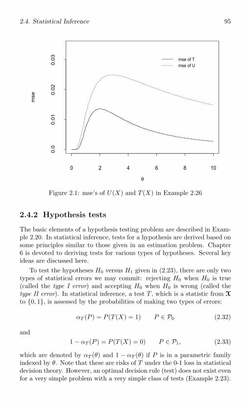
2.4. Statistical Inference 95
mse
0 2 4 6 8 10
0.0
0.01
0.02
0.03
θ
mse of Tmse of U
Figure 2.1: mse’s of U(X) and T (X) in Example 2.26
2.4.2 Hypothesis tests
The basic elements of a hypothesis testing problem are described in Exam-ple 2.20. In statistical inference, tests for a hypothesis are derived based onsome principles similar to those given in an estimation problem. Chapter6 is devoted to deriving tests for various types of hypotheses. Several keyideas are discussed here.
To test the hypotheses H0 versus H1 given in (2.23), there are only twotypes of statistical errors we may commit: rejecting H0 when H0 is true(called the type I error) and accepting H0 when H0 is wrong (called thetype II error). In statistical inference, a test T , which is a statistic from X
to 0, 1, is assessed by the probabilities of making two types of errors:
αT (P ) = P (T (X) = 1) P ∈ P0 (2.32)
and1 − αT (P ) = P (T (X) = 0) P ∈ P1, (2.33)
which are denoted by αT (θ) and 1 − αT (θ) if P is in a parametric familyindexed by θ. Note that these are risks of T under the 0-1 loss in statisticaldecision theory. However, an optimal decision rule (test) does not exist evenfor a very simple problem with a very simple class of tests (Example 2.23).
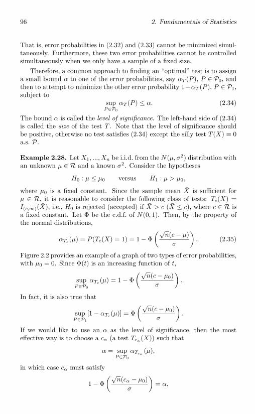
96 2. Fundamentals of Statistics
That is, error probabilities in (2.32) and (2.33) cannot be minimized simul-taneously. Furthermore, these two error probabilities cannot be controlledsimultaneously when we only have a sample of a fixed size.
Therefore, a common approach to finding an “optimal” test is to assigna small bound α to one of the error probabilities, say αT (P ), P ∈ P0, andthen to attempt to minimize the other error probability 1−αT (P ), P ∈ P1,subject to
supP∈P0
αT (P ) ≤ α. (2.34)
The bound α is called the level of significance. The left-hand side of (2.34)is called the size of the test T . Note that the level of significance shouldbe positive, otherwise no test satisfies (2.34) except the silly test T (X) ≡ 0a.s. P.
Example 2.28. Let X1, ..., Xn be i.i.d. from the N(µ, σ2) distribution withan unknown µ ∈ R and a known σ2. Consider the hypotheses
H0 : µ ≤ µ0 versus H1 : µ > µ0,
where µ0 is a fixed constant. Since the sample mean X is sufficient forµ ∈ R, it is reasonable to consider the following class of tests: Tc(X) =I(c,∞)(X), i.e., H0 is rejected (accepted) if X > c (X ≤ c), where c ∈ R isa fixed constant. Let Φ be the c.d.f. of N(0, 1). Then, by the property ofthe normal distributions,
αTc(µ) = P (Tc(X) = 1) = 1 − Φ(√
n(c− µ)σ
). (2.35)
Figure 2.2 provides an example of a graph of two types of error probabilities,with µ0 = 0. Since Φ(t) is an increasing function of t,
supP∈P0
αTc(µ) = 1 − Φ(√
n(c− µ0)σ
).
In fact, it is also true that
supP∈P1
[1 − αTc(µ)] = Φ
(√n(c− µ0)
σ
).
If we would like to use an α as the level of significance, then the mosteffective way is to choose a cα (a test Tcα(X)) such that
α = supP∈P0
αTcα(µ),
in which case cα must satisfy
1 − Φ(√
n(cα − µ0)σ
)= α,
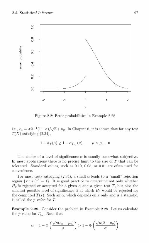
2.4. Statistical Inference 97
err
or p
roba
bilty
-2 -1 0 1 2
0.0
0.2
0.4
0.6
0.8
1.0
µ
Figure 2.2: Error probabilities in Example 2.28
i.e., cα = σΦ−1(1−α)/√n+µ0. In Chapter 6, it is shown that for any test
T (X) satisfying (2.34),
1 − αT (µ) ≥ 1 − αTcα(µ), µ > µ0.
The choice of a level of significance α is usually somewhat subjective.In most applications there is no precise limit to the size of T that can betolerated. Standard values, such as 0.10, 0.05, or 0.01 are often used forconvenience.
For most tests satisfying (2.34), a small α leads to a “small” rejectionregion x : T (x) = 1. It is good practice to determine not only whetherH0 is rejected or accepted for a given α and a given test T , but also thesmallest possible level of significance α at which H0 would be rejected forthe computed T (x). Such an α, which depends on x only and is a statistic,is called the p-value for T .
Example 2.29. Consider the problem in Example 2.28. Let us calculatethe p-value for Tcα . Note that
α = 1 − Φ(√
n(cα − µ0)σ
)> 1 − Φ
(√n(x− µ0)
σ
)
98 2. Fundamentals of Statistics
if and only if x > cα (or Tcα(x) = 1). Hence
1 − Φ(√
n(x− µ0)σ
)= infα ∈ (0, 1) : Tcα(x) = 1 = α(x)
is the p-value for Tcα . It turns out that Tcα(x) = I(0,α)(α(x)).
With the additional information provided by p-values, using p-values istypically more appropriate than using fixed-level tests in a scientific prob-lem. However, a fixed level of significance is unavoidable when acceptanceor rejection of H0 implies an imminent concrete decision. For more discus-sions about p-values, see Lehmann (1986) and Weerahandi (1995).
In Example 2.28, the equality in (2.34) can always be achieved by asuitable choice of c. This is, however, not true in general. In Example 2.23,for instance, it is possible to find an α such that
sup0<θ≤θ0
P (Tj(X) = 1) = α
for all Tj ’s. In such cases we may consider randomized tests, which areintroduced next.
Recall that a randomized decision rule is a probability measure δ(x, ·)on the action space for any fixed x. Since the action space contains onlytwo points, 0 and 1, for a hypothesis testing problem, any randomized testδ(X,A) is equivalent to a statistic T (X) ∈ [0, 1] with T (x) = δ(x, 1) and1 − T (x) = δ(x, 0). A nonrandomized test is obviously a special casewhere T (x) does not take any value in (0, 1).
For any randomized test T (X), we define the type I error probabilityto be αT (P ) = E[T (X)], P ∈ P0, and the type II error probability to be1 − αT (P ) = E[1 − T (X)], P ∈ P1. For a class of randomized tests, wewould like to minimize 1 − αT (P ) subject to (2.34).
Example 2.30. Consider Example 2.23 and the following class of random-ized tests:
Tj,q(X) =
⎧⎨⎩1 X > j
q X = j
0 X < j,
where j = 0, 1, ..., n− 1 and q ∈ [0, 1]. Then
αTj,q (θ) = P (X > j) + qP (X = j) 0 < θ ≤ θ0
and
1 − αTj,q(θ) = P (X < j) + (1 − q)P (X = j) θ0 < θ < 1.
It can be shown that for any α ∈ (0, 1), there exist integer j and q ∈ (0, 1)such that the size of Tj,q is α (exercise).
2.4. Statistical Inference 99
2.4.3 Confidence sets
Let ϑ be a real-valued unknown parameter related to the unknown popula-tion P ∈ P and C(X) ∈ BΘ depending only on the sample X, where Θ ∈ Bis the range of ϑ. If
infP∈P
P (ϑ ∈ C(X)) ≥ 1 − α, (2.36)
where α is a fixed constant in (0, 1), then C(X) is called a confidence setfor ϑ with level of significance 1 − α. The left-hand side of (2.36) is calledthe confidence coefficient of C(X), which is the highest possible level ofsignificance for C(X). A confidence set is a random element that coversthe unknown ϑ with certain probability. If (2.36) holds, then the coverageprobability of C(X) is at least 1 − α, although C(x) either covers or doesnot cover ϑ whence we observe X = x. The concept of confidence sets canbe extended to the case where ϑ is a vector of k real-valued parameters andC(X) ∈ Bk
Θin an obvious manner.
If C(X) = [ϑ(X), ϑ(X)] for a pair of statistics ϑ and ϑ, then C(X) iscalled a confidence interval for ϑ. If C(X) = (−∞, ϑ(X)] (or [ϑ(X),∞)),then ϑ (or ϑ) is called an upper (or a lower) confidence bound for ϑ. Aconfidence interval is also called an interval estimator of ϑ, although it isvery different from a point estimator (discussed in §2.4.1). The concepts oflevel of significance and confidence coefficient are very similar to the levelof significance and size in hypothesis testing. In fact, it is shown in Chapter7 that some confidence sets are closely related to hypothesis tests.
Example 2.31. Consider Example 2.28. Suppose that a confidence inter-val for ϑ = µ is needed. Again, we only need to consider ϑ(X) and ϑ(X),since the sample mean X is sufficient. Consider confidence intervals of theform [X − c, X + c], where c ∈ (0,∞) is fixed. Note that
P(µ ∈ [X − c, X + c]
)= P
(|X − µ| ≤ c
)= 1 − 2Φ
(−√nc/σ
),
which is independent of µ. Hence the confidence coefficient of [X−c, X+c]is 1−2Φ (−√
nc/σ), which is an increasing function of c and converges to 1as c → ∞ or 0 as c → 0. Thus, confidence coefficients are positive but lessthan 1 except for silly confidence intervals [X, X] and (−∞,∞). We canchoose a confidence interval with an arbitrarily small confidence coefficient,but the chosen confidence interval may be so wide that it is practicallyuseless.
If σ2 is also unknown, then [X − c, X + c] has confidence coefficient 0and, therefore, is not a good inference procedure. In such a case a differentconfidence interval for µ with positive confidence coefficient can be derived(Exercise 79 in §2.6).
100 2. Fundamentals of Statistics
This example tells us that a reasonable approach is to choose a level ofsignificance 1 − α ∈ (0, 1) (just like the level of significance in hypothesistesting) and a confidence interval or set satisfying (2.36). In Example 2.31,we may choose a confidence interval whose confidence coefficient is exactly1 − α for any fixed α ∈ (0, 1), using cα = σΦ−1(1 − α/2)/
√n. This is
desirable since, for all confidence intervals satisfying (2.36), the one withthe shortest interval length is preferred.
For a general confidence interval [ϑ(X), ϑ(X)], its length is ϑ(X)−ϑ(X),which may be random. We may consider the expected (or average) lengthE[ϑ(X)−ϑ(X)]. The confidence coefficient and expected length are a pair ofgood measures of performance of confidence intervals. Like the two typesof error probabilities of a test in hypothesis testing, however, we cannotmaximize the confidence coefficient and minimize the length (or expectedlength) simultaneously. A common approach is to minimize the length (orexpected length) subject to (2.36).
For a general confidence set C(X), the length of C(X) may be ∞. Hencewe have to define some other measures of performance. For an upper (ora lower) confidence bound, we may consider the distance ϑ(X) − ϑ (orϑ− ϑ(X)) or its expectation.
To conclude this section, we discuss an example of a confidence set fora two-dimensional parameter. General discussions about how to constructand assess confidence sets are given in Chapter 7.
Example 2.32. Let X1, ..., Xn be i.i.d. from the N(µ, σ2) distributionwith both µ ∈ R and σ2 > 0 unknown. Let θ = (µ, σ2) and α ∈ (0, 1) begiven. Let X be the sample mean and S2 be the sample variance. Since(X, S2) is sufficient (Example 2.15), we focus on C(X) which is a function of(X, S2). From Example 2.18, X and S2 are independent and (n− 1)S2/σ2
has the chi-square distribution χ2n−1. Since
√n(X − µ)/σ has the N(0, 1)
distribution (Exercise 51 in §1.6),
P
(−cα ≤ X − µ
σ/√n
≤ cα
)=
√1 − α,
where cα = Φ−1(
1+√
1−α2
)(verify). Since the chi-square distribution χ2
n−1
is a known distribution, we can always find two constants c1α and c2α suchthat
P
(c1α ≤ (n− 1)S2
σ2 ≤ c2α
)=
√1 − α.
Then
P
(−cα ≤ X − µ
σ/√n
≤ cα, c1α ≤ (n− 1)S2
σ2 ≤ c2α
)= 1 − α,
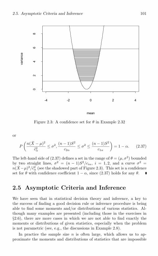
2.5. Asymptotic Criteria and Inference 101
mean
varia
nce
-4 -2 0 2 4
02
46
8
Figure 2.3: A confidence set for θ in Example 2.32
or
P
(n(X − µ)2
c2α≤ σ2,
(n− 1)S2
c2α≤ σ2 ≤ (n− 1)S2
c1α
)= 1 − α. (2.37)
The left-hand side of (2.37) defines a set in the range of θ = (µ, σ2) boundedby two straight lines, σ2 = (n − 1)S2/ciα, i = 1, 2, and a curve σ2 =n(X−µ)2/c2α (see the shadowed part of Figure 2.3). This set is a confidenceset for θ with confidence coefficient 1 − α, since (2.37) holds for any θ.
2.5 Asymptotic Criteria and Inference
We have seen that in statistical decision theory and inference, a key tothe success of finding a good decision rule or inference procedure is beingable to find some moments and/or distributions of various statistics. Al-though many examples are presented (including those in the exercises in§2.6), there are more cases in which we are not able to find exactly themoments or distributions of given statistics, especially when the problemis not parametric (see, e.g., the discussions in Example 2.8).
In practice the sample size n is often large, which allows us to ap-proximate the moments and distributions of statistics that are impossible
102 2. Fundamentals of Statistics
to derive, using the asymptotic tools discussed in §1.5. In an asymptoticanalysis, we consider a sample X = (X1, ..., Xn) not for fixed n, but as amember of a sequence corresponding to n = n0, n0 + 1, ..., and obtain thelimit of the distribution of an appropriately normalized statistic or variableTn(X) as n → ∞. The limiting distribution and their moments are used asapproximations to the distribution and moments of Tn(X) in the situationwith a large but actually finite n. This leads to some asymptotic statisticalprocedures and asymptotic criteria for assessing their performances, whichare introduced in this section.
The asymptotic approach is not only applied to the situation where noexact method is available, but also used to provide an inference proceduresimpler (e.g., in terms of computation) than that produced by the exactapproach (the approach considering a fixed n). Some examples are givenin later chapters.
In addition to providing more theoretical results and/or simpler infer-ence procedures, the asymptotic approach requires less stringent mathe-matical assumptions than does the exact approach. The mathematical pre-cision of the optimality results obtained in statistical decision theory, forexample, tends to obscure the fact that these results are approximations inview of the approximate nature of the assumed models and loss functions.As the sample size increases, the statistical properties become less depen-dent on the loss functions and models. However, a major weakness of theasymptotic approach is that typically no good estimates are available forthe precision of the approximations so that we cannot determine whethera particular n in a problem is large enough to safely apply the asymptoticresults. To overcome this difficulty, asymptotic results are frequently usedin combination with some numerical/empirical studies for selected valuesof n to examine the finite sample performance of asymptotic procedures.
2.5.1 Consistency
A reasonable point estimator is expected to perform better, at least onthe average, if more information about the unknown population is avail-able. With a fixed model assumption and sampling plan, more data (largersample size n) provide more information about the unknown population.Thus, it is distasteful to use a point estimator Tn which, if sampling wereto continue indefinitely, could possibly have a nonzero estimation error, al-though the estimation error of Tn for a fixed n may never equal 0 (see thediscussion in §2.4.1).
Definition 2.10 (Consistency of point estimators). Let X = (X1, ..., Xn)be a sample from P ∈ P and Tn(X) be a point estimator of ϑ for every n.(i) Tn(X) is called consistent for ϑ if and only if Tn(X) →p ϑ w.r.t. any
2.5. Asymptotic Criteria and Inference 103
P ∈ P.(ii) Let an be a sequence of positive constants diverging to ∞. Tn(X) iscalled an-consistent for ϑ if and only if an[Tn(X) − ϑ] = Op(1) w.r.t. anyP ∈ P.(iii) Tn(X) is called strongly consistent for ϑ if and only if Tn(X) →a.s. ϑw.r.t. any P ∈ P.(iv) Tn(X) is called Lr-consistent for ϑ if and only if Tn(X) →Lr ϑ w.r.t.any P ∈ P for some fixed r > 0.
Consistency is actually a concept relating to a sequence of estimators,Tn, n = n0, n0 + 1, ..., but we usually just say “consistency of Tn” forsimplicity. Each of the four types of consistency in Definition 2.10 describesthe convergence of Tn(X) to ϑ in some sense, as n → ∞. In statistics,consistency according to Definition 2.10(i), which is sometimes called weakconsistency since it is implied by any of the other three types of consistency,is the most useful concept of convergence of Tn to ϑ. L2-consistency is alsocalled consistency in mse, which is the most useful type of Lr-consistency.
Example 2.33. Let X1, ..., Xn be i.i.d. from P ∈ P. If ϑ = µ, whichis the mean of P (assumed to be finite), then by the SLLN (Theorem1.13), the sample mean X is strongly consistent for µ and, therefore, isalso consistent for µ. If we further assume that the variance of P is finite,then by (2.22), X is consistent in mse and is
√n-consistent. With the finite
variance assumption, the sample variance S2 is strongly consistent for thevariance of P , according to the SLLN.
Consider estimators of the form Tn =∑n
i=1 cinXi, where cin is adouble array of constants. If P has a finite variance, then by (2.27), Tn
is consistent in mse if and only if∑n
i=1 cin → 1 and∑n
i=1 c2in → 0. If we
only assume the existence of the mean of P , then Tn with cin = ci/n sat-isfying n−1 ∑n
i=1 ci → 1 and supi |ci| < ∞ is strongly consistent (Theorem1.13(ii)).
One or a combination of the law of large numbers, the CLT, Slutsky’stheorem (Theorem 1.11), and the continuous mapping theorem (Theorems1.10 and 1.12) are typically applied to establish consistency of point estima-tors. In particular, Theorem 1.10 implies that if Tn is (strongly) consistentfor ϑ and g is a continuous function of ϑ, then g(Tn) is (strongly) consistentfor g(ϑ). For example, in Example 2.33 the point estimator X2 is stronglyconsistent for µ2. To show that X2 is
√n-consistent under the assumption
that P has a finite variance σ2, we can use the identity√n(X2 − µ2) =
√n(X − µ)(X + µ)
and the fact that X is√n-consistent for µ and X + µ = Op(1). (Note that
104 2. Fundamentals of Statistics
X2 may not be consistent in mse since we do not assume that P has a finitefourth moment.) Alternatively, we can use the fact that
√n(X2 − µ2) →d
N(0, 4µ2σ2) (by the CLT and Theorem 1.12) to show the√n-consistency
of X2.The following example shows another way to establish consistency of
some point estimators.
Example 2.34. Let X1, ..., Xn be i.i.d. from an unknown P with a con-tinuous c.d.f. F satisfying F (θ) = 1 for some θ ∈ R and F (x) < 1 for anyx < θ. Consider the largest order statistic X(n). For any ε > 0, F (θ−ε) < 1and
P (|X(n) − θ| ≥ ε) = P (X(n) ≤ θ − ε) = [F (θ − ε)]n ,
which imply (according to Theorem 1.8(v)), X(n) →a.s. θ, i.e., X(n) isstrongly consistent for θ. Let F (i)(θ−) be the ith order left-hand derivativeof F at θ. If we assume that F (i)(θ−), i = 1, ...,m, exist and vanish, andthat F (m+1)(θ−) exists and is nonzero, then
1 − F (X(n)) =F (m+1)(θ−)
(m + 1)!(θ −X(n))m+1 + o
(|θ −X(n)|m+1) a.s.
Let
hn(θ) =[
(m + 1)!nF (m+1)(θ−)
](m+1)−1
.
For any t ≤ 0, by Slutsky’s theorem,
limn→∞
P
(X(n) − θ
hn(θ)≤ t
)= lim
n→∞P
([θ −X(n)
hn(θ)
]m+1
≥ (−t)m+1
)= lim
n→∞P
(n[1 − F (X(n))] ≥ (−t)m+1)
= limn→∞
[1 − (−t)m+1/n
]n= e−(−t)m+1
.
This shows that (X(n) − θ)/hn(θ) →d Y , where Y is a random variablehaving the c.d.f. e−(−t)m+1
I(−∞,0)(t). Thus, X(n) is n(m+1)−1-consistent. If
m = 0, then X(n) is n-consistent, which is the most common situation. Ifm = 1, then X(n) is
√n-consistent.
It can be seen from the previous examples that there are many consistentestimators. Like the admissibility in statistical decision theory, consistencyis a very essential requirement in the sense that any inconsistent estimatorsshould not be used, but a consistent estimator is not necessarily good.Thus, consistency should be used together with one or a few more criteria.
2.5. Asymptotic Criteria and Inference 105
We now discuss a situation in which finding a consistent estimator iscrucial. Suppose that an estimator Tn of ϑ satisfies
cn[Tn(X) − ϑ] →d σY, (2.38)
where Y is a random variable with a known distribution, σ > 0 is anunknown parameter, and cn is a sequence of constants; for example, inExample 2.33,
√n(X − µ) →d N(0, σ2); in Example 2.34, (2.38) holds
with cn = n(m+1)−1and σ = [(−1)m(m + 1)!/F (m+1)(θ−)](m+1)−1
. If aconsistent estimator σn of σ can be found, then, by Slutsky’s theorem,
cn[Tn(X) − ϑ]/σn →d Y
and, thus, we may approximate the distribution of cn[Tn(X) − ϑ]/σn bythe known distribution of Y .
2.5.2 Asymptotic bias, variance, and mse
Unbiasedness as a criterion for point estimators is discussed in §2.3.2 and§2.4.1. In some cases, however, there is no unbiased estimator (Exercise 69in §2.6). Furthermore, having a “slight” bias in some cases may not be abad idea (see Exercise 52 in §2.6). Let Tn(X) be a point estimator of ϑ forevery n and an be a sequence of positive numbers satisfying an → ∞ oran → a > 0. If ETn exists for every n and limn→∞ anE(Tn − ϑ) = 0 forany P ∈ P, then Tn is called an-approximately unbiased or approximatelyunbiased if an ≡ 1.
There are many reasonable point estimators whose expectations arenot well defined. For example, consider i.i.d. (X1, Y1), ..., (Xn, Yn) from abivariate normal distribution with µx = EX1 and µy = EY1 = 0. Letϑ = µx/µy and Tn = X/Y , the ratio of two sample means. Then ETn isnot defined for any n. It is then desirable to define a concept of asymptoticbias for point estimators whose expectations are not well defined.
Definition 2.11. Let ξn, γn, and εn be sequences of random vari-ables such that Pξn = Pγn+εn for any n; Eγn exists for any n; εn = op(1);and
limn→∞
P (|εn| ≥ ε|γn|, γn = 0) = 0 for any ε > 0. (2.39)
Then Eγn is called an asymptotic expectation of ξn.
Note that asymptotic expectations of ξn, in most cases, are not unique.The following results can be used to find asymptotic expectations.
Proposition 2.3. Let ξn, γn, and εn be sequences of random vari-ables given in Definition 2.11.
106 2. Fundamentals of Statistics
(i) If ξn = γn + εn, then Eγn is an asymptotic expectation of ξn.(ii) Let an be a sequence of positive numbers satisfying an → ∞ oran → a > 0. If anξn →d Y , where Y is a random variable with E|Y | < ∞,then EY/an is an asymptotic expectation of ξn.Proof. (i) is obvious. We now show (ii). According to Theorem 1.8(iv),anξn →d Y implies that there are ζn and Z such that Pζn = Panξn ,n = 1, 2, ..., PZ = PY , and ζn = Z + op(1). Letting γn = Z/an andεn = (ζn −Z)/an, the result follows from Definition 2.11 and the fact thatEZ = EY .
Let Tn(X) be a point estimator of ϑ for every n and bTn(P ) be an
asymptotic expectation of Tn−ϑ. Then bTn(P ) is called an asymptotic biasof Tn and is denoted by bTn(θ) if P is in a parametric family. Note that ifthe exact bias bTn
(P ) exists, then it is an asymptotic bias of Tn. Let anbe a sequence of positive numbers satisfying an → ∞ or an → a > 0. Iflimn→∞ anbTn(P ) = 0 for any P ∈ P, then Tn is called an-asymptoticallyunbiased or asymptotically unbiased if an ≡ 1.
If Tn is a consistent estimator of ϑ, then Tn = ϑ+ op(1) and, by Propo-sition 2.3, Tn is asymptotically unbiased, although Tn may not be approxi-mately unbiased; in fact, g(Tn) is asymptotically unbiased for g(ϑ) for anycontinuous function g. For the example of Tn = X/Y , Tn →a.s. µx/µy bythe SLLN. Hence Tn is asymptotically unbiased, although ETn may not bedefined.
It follows from Proposition 2.3 that in Example 2.34, X(n) has an asymp-totic bias bTn
(P ) = hn(θ)EY , which is of order n−(m+1)−1; in Example 2.33,
X2 is√n-asymptotically unbiased. A more precise result about the asymp-
totic bias of X2 can be obtained using the following result for functions ofunbiased estimators.
Theorem 2.6. Let g be a function on Rk which is second-order differen-tiable at θ ∈ Rk. Suppose that Ujn is an unbiased estimator of the jthcomponent of θ, Var(Ujn) < ∞, j = 1, ..., k, and Un − θ = op(1), whereUn = (U1n, ..., Ukn). Then an asymptotic bias of Tn = g(Un) as an esti-mator of ϑ = g(θ) is tr(∇2g(θ)Var(Un))/2, where tr(M) is the trace of amatrix M and ∇2g(θ) is the matrix of second-order partial derivatives of gat θ.Proof. Using Taylor’s expansion and the fact that Un − θ = op(1),
Tn − ϑ = γn + εn,
whereγn = ∇g(θ)(Un − θ)τ + 1
2 (Un − θ)∇2g(θ)(Un − θ)τ ,
∇g(θ) denotes the k-vector of partial derivatives of g at θ, and εn satisfies
2.5. Asymptotic Criteria and Inference 107
(2.39). The result follows from EUn = θ and
E[(Un − θ)∇2g(θ)(Un − θ)τ
]= tr
(∇2g(θ)E(Un − θ)τ (Un − θ)
).
Theorem 2.6 can be applied to the case where Un is the k-vector ofsample means, i.e., Un = X = n−1 ∑n
i=1 Xi with i.i.d. random k-vectorsX1, ..., Xn. A similar result for the exact bias of g(X) is given in Lehmann(1983, Theorem 2.5.1), which requires a much more stringent condition onthe derivatives of g.
Example 2.35. Let X1, ..., Xn be i.i.d. binary random variables withP (Xi = 1) = p, where p ∈ (0, 1) is unknown. Consider first the esti-mation of ϑ = p(1 − p). Since the sample mean X is unbiased for p withVar(X) = p(1 − p)/n, an asymptotic bias of Tn = X(1 − X) according toTheorem 2.6 with g(x) = x(1−x) is −p(1−p)/n. On the other hand, a di-rect computation shows E[X(1−X)] = EX−EX2 = p−(EX)2−Var(X) =p(1 − p) − p(1 − p)/n. Hence the exact bias of Tn is −p(1 − p)/n, which isthe same as the asymptotic bias obtained previously.
Consider next the estimation of ϑ = p−1. In this case there is nounbiased estimator of p−1 (Exercise 69 in §2.6). Let Tn = X−1. Thenan asymptotic bias of Tn according to Theorem 2.6 with g(x) = x−1 is(1 − p)/(pn). On the other hand, ETn = ∞ for every n.
Like the bias, the mse of an estimator Tn of ϑ is not well defined if thesecond moment of Tn does not exist. Thus, an asymptotic expectation of(Tn − ϑ)2 is defined to be an asymptotic mean squared error (amse) of Tn,which is denoted by amseTn(P ) or amseTn(θ) if P is in a parametric familyindexed by θ. An asymptotic variance of Tn is defined to be
σ2Tn
(P ) = amseTn(P ) − [bTn(P )]2.
In many problems [bTn(P )]2/amseTn(P ) = o(1), in which case asymptoticvariances are the same as amse’s.
If an(Tn − ϑ) →d Y with 0 < EY 2 < ∞, then by Proposition 2.3,amseTn
(P ) = EY 2/a2n, and σ2
Tn(P ) = Var(Y )/a2
n. For instance, in Exam-ple 2.34, σ2
X(n)(P ) = [hn(θ)]2Var(Y ) and amseX(n)(P ) = [hn(θ)]2EY 2; in
Example 2.33, amseX2(P ) = σ2X2(P ) = 4µ2σ2/n.
Since amse’s of an estimator are not unique, it is not suitable to usethem to assess and compare different estimators. Two estimators T1n andT2n may satisfy limn→∞[amseT1n(P )/amseT2n(P )] < 1 for one version ofamse’s, whereas limn→∞[amseT1n(P )/amseT2n(P )] > 1 for another versionof amse’s (Exercise 97 in §2.6). Thus, we need the following definition.
108 2. Fundamentals of Statistics
Definition 2.12. Let Tn be an estimator of ϑ for every n and Eγ2n be an
amse of Tn.(i) Suppose that there is a sequence of positive numbers an such thatan → ∞ and
limt→∞
limn→∞
E[min(a2nγ
2n, t)] = lim
n→∞a2nEγ2
n ∈ (0,∞). (2.40)
Then Eγ2n is called a regular amse of Tn and is denoted by amseTn
(P ).(ii) Let T ′
n be another estimator of ϑ. The asymptotic relative efficiency ofT ′n w.t.r. Tn is defined to be
eT ′n,Tn(P ) = amseTn
(P )/amseT ′n(P ).
(iii) Tn is said to be asymptotically more efficient than T ′n if and only if
lim supn eT ′n,Tn
(P ) < 1 for any P .
The following result shows that the regular amse is unique in the limitingsense so that the concepts of asymptotic relative efficiency in Definition2.12(ii)-(iii) are well defined. It also shows how to find regular amse’s andasymptotic relative efficiencies.
Proposition 2.4. Let Tn be an estimator of ϑ for every n and rn =amseTn
(P ) with limn→∞ a2nrn ∈ (0,∞).
(i) If r′n is another amse of Tn, then lim infn(r′n/rn) ≥ 1.(ii) If both rn and r′n are regular amse’s of Tn, then limn→∞(rn/r′n) = 1.(iii) If cn(Tn − ϑ) →d Y for a random variable Y with 0 < EY 2 < ∞ anda sequence cn of positive numbers satisfying cn → ∞, then EY 2/c2n =amseTn
(P ).Proof. The result in (ii) follows from (i) and the result in (iii) followsdirectly from Definition 2.12. We only need to prove (i). By definition,there exist γn and γ′
n such that rn = Eγ2n, r′n = E(γ′
n)2, and P(γ′n)2 =
Pγ2n[1+op(1)]. Since
min(anγn)2[1 + op(1)], t − min(anγn)2, t = op(1)
for any t > 0 and min[(anγ′n)2, t] and min[(anγn)2, t] are bounded by t,
Emin[(anγ′n)2, t] = Emin[(anγn)2, t] + o(1),
which with (2.40) implies that
limt→∞
limn→∞
Emin[(anγ′n)2, t] = lim
n→∞a2nEγ2
n.
The result follows from
limt→∞
limn→∞
Emin[(anγ′n)2, t] ≤ lim inf
nE(anγ′
n)2.
2.5. Asymptotic Criteria and Inference 109
It follows from Proposition 2.4 that if mseTn(P ) exists, then
lim infn
[mseTn(P )/amseTn(P )] ≥ 1,
since mseTn(P ) is a particular amse of Tn. It is often true that mseTn(P ) =amseTn
(P ), which is implied by the uniform integrability of a2n(Tn − ϑ)2
for an in Definition 2.12 (exercise).
Example 2.36. Let X1, ..., Xn be i.i.d. from the Poisson distribution P (θ)with an unknown θ > 0. Consider the estimation of ϑ = P (Xi = 0) = e−θ.Let T1n = Fn(0), where Fn is the empirical c.d.f. defined in (2.31). ThenT1n is unbiased and has mseT1n(θ) = e−θ(1 − e−θ)/n. It can be shownthat n2E[T1n − F (0)]4 is bounded. Hence n[T1n − F (0)]2 is uniformlyintegrable and, therefore, amseT1n
(θ) = mseT1n(θ).
Next, consider T2n = e−X . Note that ET2n = enθ(e−1/n−1). Hence
nbT2n(θ) → θe−θ/2. Using Theorem 1.12 and the CLT, we can show that
√n(T2n − ϑ) →d N(0, e−2θθ).
By Proposition 2.4(iii), amseT2n(θ) = e−2θθ/n. Thus, the asymptotic rela-
tive efficiency of T1n w.r.t. T2n is
eT1n,T2n(θ) = θ/(eθ − 1),
which is always less than 1. This shows that T2n is asymptotically moreefficient than T1n.
The result for T2n in Example 2.36 is a special case (with Un = X) ofthe following general result.
Theorem 2.7. Let g be a function on Rk which is differentiable at θ ∈ Rk
and let Un be a k-vector of statistics satisfying that Un − θ = op(1) andE‖Un − θ‖2 < ∞. Let Tn = g(Tn) be an estimator of ϑ = g(θ). Then(i) σ2
Tn(P ) = ∇g(θ)Var(Un)[∇g(θ)]τ and amseTn(P ) = E[∇g(θ)(Un−θ)τ ]2;
(ii) amseTn(P ) = E[∇g(θ)Y τ ]2/c2n if cn(Un−θ) →d Y for a random k-vector
Y with 0 < E‖Y ‖2 < ∞.
2.5.3 Asymptotic inference
Statistical inference based on asymptotic criteria and approximations iscalled asymptotic statistical inference or simply asymptotic inference. Wehave previously considered asymptotic estimation. We now focus on asymp-totic hypothesis tests and confidence sets.
110 2. Fundamentals of Statistics
Definition 2.13. Let X = (X1, ..., Xn) be a sample from P ∈ P andTn(X) be a test for H0 : P ∈ P0 versus H1 : P ∈ P1.(i) If lim supn αTn(P ) ≤ α for any P ∈ P0, then α is an asymptotic signifi-cance level of Tn.(ii) If limn→∞ supP∈P0
αTn(P ) exists, then it is called the limiting size ofTn.(iii) Tn is called consistent if and only if the type II error probability con-verges to 0, i.e., limn→∞[1 − αTn(P )] = 0, for any P ∈ P1.(iv) Tn is called Chernoff-consistent if and only if Tn is consistent and thetype I error probability converges to 0, i.e., limn→∞ αTn(P ) = 0, for anyP ∈ P0. Tn is called uniformly Chernoff-consistent if and only if Tn isconsistent and the limiting size of Tn is 0.
Obviously if Tn has size (or significance level) α for all n, then its limitingsize (or asymptotic significance level) is α. If the limiting size of Tn isα ∈ (0, 1), then for any ε > 0, Tn has size α + ε for all n ≥ n0, where n0 isindependent of P . Hence Tn has level of significance α + ε for any n ≥ n0.However, if P0 is not a parametric family, it is likely that the limiting sizeof Tn is 1 (see, e.g., Example 2.37). This is the reason why we consider theweaker requirement in Definition 2.13(i). If Tn has asymptotic significancelevel α, then for any ε > 0, αTn(P ) < α + ε for all n ≥ n0(P ) but n0(P )depends on P ∈ P0; and there is no guarantee that Tn has significance levelα + ε for any n.
The consistency in Definition 2.13(iii) only requires that the type II er-ror probability converge to 0. We may define uniform consistency to belimn→∞ supP∈P1
[1 − αTn(P )] = 0, but it is not satisfied in most problems.If α ∈ (0, 1) is a pre-assigned level of significance for the problem, then aconsistent test Tn having asymptotic significance level α is called asymptot-ically correct, and a consistent test having limiting size α is called stronglyasymptotically correct.
The Chernoff-consistency (or uniformly Chernoff-consistency) in Defi-nition 2.13(iv) requires that both types of error probabilities converge to0. Mathematically, Chernoff-consistency (or uniform Chernoff-consistency)is better than asymptotic correctness (or strongly asymptotic correctness).After all, both types of error probabilities should decrease to 0 if samplingcan be continued indefinitely. However, if α is chosen to be small enough sothat error probabilities smaller than α can be practically treated as 0, thenthe asymptotic correctness (or strongly asymptotic correctness) is enough,and is probably preferred, since requiring an unnecessarily small type Ierror probability usually results in an unnecessary increase in the type IIerror probability as the following example illustrates.
Example 2.37. Consider the testing problem H0 : µ ≤ µ0 versus H1 :
2.5. Asymptotic Criteria and Inference 111
µ > µ0 based on i.i.d. X1, ..., Xn with EX1 = µ ∈ R. If each Xi has theN(µ, σ2) distribution with a known σ2, then the test Tcα given in Example2.28 with cα = σ−1Φ−1(1 − α)/
√n + µ0 and α ∈ (0, 1) has size α (and,
therefore, limiting size α). It also follows from (2.35) that for any µ > µ0,
1 − αTcα(µ) = Φ
(Φ−1(1 − α) +
√n(µ0 − µ)
σ
)→ 0 (2.41)
as n → ∞. This shows that Tcα is consistent and, hence, is stronglyasymptotically correct. Note that the convergence in (2.41) is not uniformin µ > µ0, but is uniform in µ > µ1 for any fixed µ1 > µ0.
Since the size of Tcα is α for all n, Tcα is not Chernoff-consistent. Auniformly Chernoff-consistent test can be obtained as follows. Let α(n) ⊂(0, 1) be a sequence satisfying α(n) → 0 and
√nα(n) → ∞. Then Tcα(n)
has size α(n) for each n and, therefore, its limiting size is 0. On the otherhand, (2.41) still holds with α replaced by α(n) (exercise). Hence Tcα(n)
is uniformly Chernoff-consistent. However, if α(n) < α, then, from theleft-hand side of (2.41), 1 − αTcα
(µ) < 1 − αTcα(n)(µ) for any µ > µ0.
We now consider the case where the population P is not in a parametricfamily. We still assume that σ2 = Var(Xi) is known. Using the CLT, wecan show that for µ > µ0,
limn→∞
[1 − αTcα(µ)] = lim
n→∞Φ
(Φ−1(1 − α) +
√n(µ0 − µ)
σ
)= 0,
i.e., Tcα is still consistent. For µ ≤ µ0,
limn→∞
αTcα(µ) = 1 − lim
n→∞Φ
(Φ−1(1 − α) +
√n(µ0 − µ)
σ
),
which equals α if µ = µ0 and 0 if µ < µ0. Thus, the asymptotic signifi-cance level of Tcα is α. Combining these two results, we know that Tcα isasymptotically correct. However, if P contains all possible populations onR, then one can show that the limiting size of Tcα is 1 (exercise). Usingthe same argument that is used for the normal case, we can also show thatTcα(n) is Chernoff-consistent if α(n) → 0 and
√nα(n) → ∞. But Tcα(n) is
not uniformly Chernoff-consistent if P contains all possible populations onR.
Definition 2.14. Let ϑ be a k-vector of parameters related to the unknownpopulation P ∈ P and C(X) be a confidence set for ϑ.(i) If lim infn P (ϑ ∈ C(X)) ≥ 1 − α for any P ∈ P, then 1 − α is anasymptotic significance level of C(X).(ii) If limn→∞ infP∈P P (ϑ ∈ C(X)) exists, then it is called the limitingconfidence coefficient of C(X).
112 2. Fundamentals of Statistics
Note that the asymptotic significance level and limiting confidence co-efficient of a confidence set are very similar to the asymptotic significancelevel and limiting size of a test, respectively. Some conclusions are also sim-ilar. For example, in a parametric problem one can often find a confidenceset having limiting confidence coefficient 1 − α ∈ (0, 1), which implies thatfor any ε > 0, the confidence coefficient of C(X) is 1−α− ε for all n ≥ n0,where n0 is independent of P ; in a nonparametric problem the limitingconfidence coefficient of C(X) might be 0, whereas C(X) may have asymp-totic significance level 1 − α ∈ (0, 1), but for any fixed n, the confidencecoefficient of C(X) might be 0.
The confidence interval in Example 2.31 with c = σΦ−1(1 − α/2)/√n
and the confidence set in Example 2.32 have confidence coefficient 1−α forany n and, therefore, have limiting confidence coefficient 1 − α. If we dropthe normality assumption and assume EX4
i < ∞, then these confidence setshave asymptotic significance level 1−α; their limiting confidence coefficientsmay be 0 (exercise).
2.6 Exercises
1. Consider Example 2.3. Suppose that p(s) is constant. Show thatXi and Xj , i = j, are not uncorrelated and, hence, X1, ..., Xn arenot independent. Furthermore, if yi’s are either 0 or 1, show thatZ =
∑ni=1 Xi has a hypergeometric distribution and compute the
mean of Z.
2. Consider Example 2.3. Suppose that we do not require that the ele-ments in s be distinct, i.e., we consider sampling with replacement.Define a suitable sample space Ω, a σ-field on Ω, a probability measurep on (Ω,F), and a sample (X1, ..., Xn) such that (2.3) holds. If p(s) isconstant, are X1, ..., Xn independent? If p(s) is constant and yi’s areeither 0 or 1, what are the distribution and mean of Z =
∑ni=1 Xi?
3. Show that Pθ : θ ∈ Θ is an exponential family and find its canonicalform, Ξ, and natural parameter space, when(a) Pθ is the Poisson distribution P (θ), θ ∈ Θ = (0,∞);(b) Pθ is the negative binomial distribution NB(θ, r) with a fixed r,θ ∈ Θ = (0, 1);(c) Pθ is the exponential distribution E(a, θ) with a fixed a, θ ∈ Θ =(0,∞);(d) Pθ is the gamma distribution Γ(α, γ), θ = (α, γ) ∈ Θ = (0,∞) ×(0,∞);(e) Pθ is the beta distribution B(α, β), θ = (α, β) ∈ Θ = (0, 1)×(0, 1);
2.6. Exercises 113
(f) Pθ is the Weibull distribution W (α, θ) with a fixed α > 0, θ ∈ Θ =(0,∞).
4. Show that the family of exponential distributions E(a, θ) with twounknown parameters a and θ is not an exponential family.
5. Show that the family of negative binomial distributions NB(p, r) withtwo unknown parameters p and r is not an exponential family.
6. Show that the family of Cauchy distributions C(µ, σ) with two un-known parameters µ and σ is not an exponential family.
7. Show that the family of Weibull distributions W (α, θ) with two un-known parameters α and θ is not an exponential family.
8. Is the family of log-normal distributions LN(µ, σ2) with two unknownparameters µ and σ2 an exponential family?
9. Show that the family of double exponential distributions DE(µ, θ)with two unknown parameters µ and θ is not an exponential family,but the family of double exponential distributions DE(µ, θ) with afixed µ and an unknown parameter θ is an exponential family.
10. Show that the k-dimensional normal family discussed in Example 2.4is an exponential family. Identify the functions T , η, ξ, and h.
11. Obtain the variance-covariance matrix for (X1, ..., Xk) in Example2.7, using (a) Theorem 2.1(ii) and (b) direct computation.
12. Show that the m.g.f. of the gamma distribution Γ(α, γ) is (1− γt)−α,t < γ−1, using Theorem 2.1(ii).
13. A discrete random variable X with
P (X = x) = γ(x)θx/c(θ), x = 0, 1, 2, ...,
where γ(x) ≥ 0, θ > 0, and c(θ) =∑∞
x=0 γ(x)θx, is called a randomvariable with a power series distribution. Show that power seriesdistributions with θ > 0 form an exponential family and obtain them.g.f. of X.
14. Let X be a random variable with a p.d.f. fθ in an exponential familyPθ : θ ∈ Θ and let A be an event. Show that the distribution ofX truncated on A has a p.d.f. fθIA/Pθ(A) which is in an exponentialfamily.
114 2. Fundamentals of Statistics
15. Let P(µ,Σ) : µ ∈ Rk,Σ ∈ Mk be a location-scale family on Rk.Suppose that P(0,Ik) has a Lebesgue p.d.f. which is always positiveand that the mean and variance-covariance matrix of P(0,Ik) are 0and Ik, respectively. Show that the mean and variance-covariancematrix of P(µ,Σ) are µ and Σ, respectively.
16. Show that if the distribution of a positive random variable X is in ascale family, then the distribution of logX is in a location family.
17. Let X be a random variable having the gamma distribution Γ(α, γ)with a known α and an unknown γ > 0 and let Y = σ logX.(a) Show that if σ > 0 is unknown, then the distribution of Y is in alocation-scale family.(b) Show that if σ > 0 is known, then the distribution of Y is in anexponential family.
18. Let X1, ..., Xn be i.i.d. random variables having a finite E|X1|4 andlet X and S2 be the sample mean and variance defined by (2.1) and(2.2). Express E(X3), Cov(X, S2), and Var(S2) in terms of αk =EXk
1 , k = 1, 2, 3, 4. Find a condition under which X and S2 areuncorrelated.
19. Let Xi = (Yi, Zi), i = 1, ..., n, be i.i.d. random 2-vectors. The statisticT (X) = (n−1)−1 ∑n
i=1(Yi− Y )(Zi− Z)/√S2Y S
2Z is called the sample
correlation coefficient, where Y = n−1 ∑ni=1 Yi and Z = n−1 ∑n
i=1 Zi
are two sample means, and S2Y = (n− 1)−1 ∑n
i=1(Yi − Y )2 and S2Z =
(n− 1)−1 ∑ni=1(Zi − Z)2 are two sample variances.
(a) Assume that E|Yi|4 < ∞ and E|Zi|4 < ∞. Show that√n[T (X) − ρ] →d N(0, c2),
where ρ is the correlation coefficient between Y1 and Z1 and c is aconstant.(b) Assume that Yi and Zi are independently distributed as N(µ1, σ
21)
and N(µ2, σ22), respectively. Show that T has the following Lebesgue
p.d.f.:
f(t) =Γ(n−1
2
)√πΓ
(n−2
2
) (1 − t2)(n−4)/2I(−1,1)(t).
(c) Assume the conditions in (b). Obtain the result in (a) usingScheffe’s theorem.
20. Prove the claims in Example 2.9 for the distributions related to orderstatistics.
21. Let X1, ..., Xn be i.i.d. random variables having the exponential dis-tribution E(a, θ), a ∈ R, and θ > 0. Show that the smallest order
2.6. Exercises 115
statistic, X(1), has the exponential distribution E(a, θ/n) and that2∑n
i=1(Xi −X(1))/θ has the chi-square distribution χ22n−2.
22. Show that if T is a sufficient statistic and T = h(S), where h ismeasurable and S is another statistic, then S is sufficient.
23. In the proof of Theorem 2.2,(a) show that C0 ∈ C;(b) show that P is dominated by Q when ν is σ-finite;(c) show that (2.12) holds.
24. Let X1, ..., Xn be i.i.d. random variables from Pθ ∈ Pθ : θ ∈ Θ.Find a sufficient statistic for θ ∈ Θ in the following cases.(a) Pθ is the Poisson distribution P (θ), θ ∈ (0,∞).(b) Pθ is the negative binomial distribution NB(θ, r) with a knownr, θ ∈ (0, 1).(c) Pθ is the exponential distribution E(0, θ), θ ∈ (0,∞).(d) Pθ is the gamma distribution Γ(α, γ), θ = (α, γ) ∈ (0,∞)×(0,∞).(e) Pθ is the beta distribution B(α, β), θ = (α, β) ∈ (0, 1) × (0, 1).(f) Pθ is the log-normal distribution LN(µ, σ2), θ = (µ, σ2) ∈ R ×(0,∞).(g) Pθ is the Weibull distribution W (α, θ) with a known α > 0, θ ∈(0,∞).
25. Let X1, ..., Xn be i.i.d. random variables from P(a,θ), where (a, θ) ∈ R2
is a parameter. Find a sufficient statistic for (a, θ) in the followingcases.(a) P(a,θ) is the exponential distribution E(a, θ), a ∈ R, θ ∈ (0,∞).(b) P(a,θ) is the Pareto distribution Pa(a, θ), a ∈ (0,∞), θ ∈ (0,∞).
26. In Example 2.11, show that X(1) (or X(n)) is sufficient for a (or b) ifwe consider a subfamily f(a,b) : a < b with a fixed b (or a).
27. Let X1, ..., Xn be i.i.d. random variables having a distribution P ∈P, where P is the family of distributions on R having continuousc.d.f.’s. Let T = (X(1), ..., X(n)) be the vector of order statistics.Show that given T , the conditional distribution of X = (X1, ..., Xn) isa discrete distribution putting probability 1/n! on each of the n! points(Xi1 , ..., Xin) ∈ Rn, where i1, ..., in is a permutation of 1, ..., n;hence, T is sufficient for P ∈ P.
28. Let X be a sample from P ∈ P containing p.d.f.’s fP
w.r.t. a σ-finitemeasure. Suppose that there is a statistic T (X) such that, for anytwo sample points x and y, f
P(x) = f
P(y)ψ(x, y) for all P and some
measurable function ψ if and only if T (x) = T (y). Show that if S(X)is a statistic sufficient for P ∈ P, then T (X) = h(S(X)) a.s. P forsome function h.
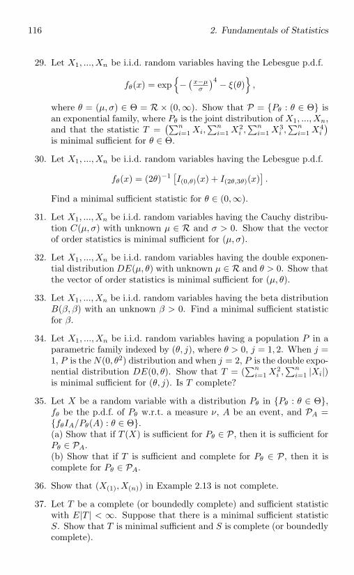
116 2. Fundamentals of Statistics
29. Let X1, ..., Xn be i.i.d. random variables having the Lebesgue p.d.f.
fθ(x) = exp−
(x−µσ
)4 − ξ(θ),
where θ = (µ, σ) ∈ Θ = R× (0,∞). Show that P = Pθ : θ ∈ Θ isan exponential family, where Pθ is the joint distribution of X1, ..., Xn,and that the statistic T =
(∑ni=1 Xi,
∑ni=1 X
2i ,
∑ni=1 X
3i ,
∑ni=1 X
4i
)is minimal sufficient for θ ∈ Θ.
30. Let X1, ..., Xn be i.i.d. random variables having the Lebesgue p.d.f.
fθ(x) = (2θ)−1 [I(0,θ)(x) + I(2θ,3θ)(x)
].
Find a minimal sufficient statistic for θ ∈ (0,∞).
31. Let X1, ..., Xn be i.i.d. random variables having the Cauchy distribu-tion C(µ, σ) with unknown µ ∈ R and σ > 0. Show that the vectorof order statistics is minimal sufficient for (µ, σ).
32. Let X1, ..., Xn be i.i.d. random variables having the double exponen-tial distribution DE(µ, θ) with unknown µ ∈ R and θ > 0. Show thatthe vector of order statistics is minimal sufficient for (µ, θ).
33. Let X1, ..., Xn be i.i.d. random variables having the beta distributionB(β, β) with an unknown β > 0. Find a minimal sufficient statisticfor β.
34. Let X1, ..., Xn be i.i.d. random variables having a population P in aparametric family indexed by (θ, j), where θ > 0, j = 1, 2. When j =1, P is the N(0, θ2) distribution and when j = 2, P is the double expo-nential distribution DE(0, θ). Show that T = (
∑ni=1 X
2i ,
∑ni=1 |Xi|)
is minimal sufficient for (θ, j). Is T complete?
35. Let X be a random variable with a distribution Pθ in Pθ : θ ∈ Θ,fθ be the p.d.f. of Pθ w.r.t. a measure ν, A be an event, and PA =fθIA/Pθ(A) : θ ∈ Θ.(a) Show that if T (X) is sufficient for Pθ ∈ P, then it is sufficient forPθ ∈ PA.(b) Show that if T is sufficient and complete for Pθ ∈ P, then it iscomplete for Pθ ∈ PA.
36. Show that (X(1), X(n)) in Example 2.13 is not complete.
37. Let T be a complete (or boundedly complete) and sufficient statisticwith E|T | < ∞. Suppose that there is a minimal sufficient statisticS. Show that T is minimal sufficient and S is complete (or boundedlycomplete).
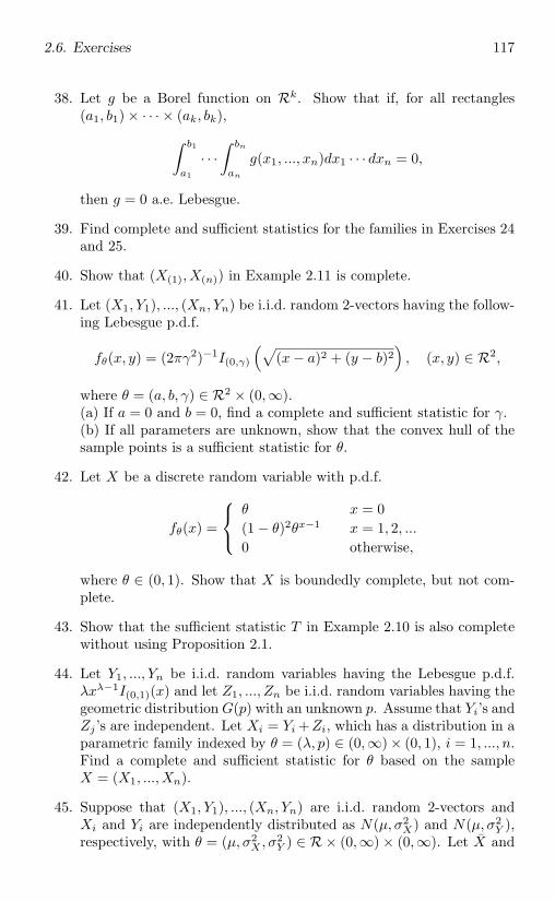
2.6. Exercises 117
38. Let g be a Borel function on Rk. Show that if, for all rectangles(a1, b1) × · · · × (ak, bk),∫ b1
a1
· · ·∫ bn
an
g(x1, ..., xn)dx1 · · · dxn = 0,
then g = 0 a.e. Lebesgue.
39. Find complete and sufficient statistics for the families in Exercises 24and 25.
40. Show that (X(1), X(n)) in Example 2.11 is complete.
41. Let (X1, Y1), ..., (Xn, Yn) be i.i.d. random 2-vectors having the follow-ing Lebesgue p.d.f.
fθ(x, y) = (2πγ2)−1I(0,γ)
(√(x− a)2 + (y − b)2
), (x, y) ∈ R2,
where θ = (a, b, γ) ∈ R2 × (0,∞).(a) If a = 0 and b = 0, find a complete and sufficient statistic for γ.(b) If all parameters are unknown, show that the convex hull of thesample points is a sufficient statistic for θ.
42. Let X be a discrete random variable with p.d.f.
fθ(x) =
⎧⎨⎩θ x = 0(1 − θ)2θx−1 x = 1, 2, ...0 otherwise,
where θ ∈ (0, 1). Show that X is boundedly complete, but not com-plete.
43. Show that the sufficient statistic T in Example 2.10 is also completewithout using Proposition 2.1.
44. Let Y1, ..., Yn be i.i.d. random variables having the Lebesgue p.d.f.λxλ−1I(0,1)(x) and let Z1, ..., Zn be i.i.d. random variables having thegeometric distribution G(p) with an unknown p. Assume that Yi’s andZj ’s are independent. Let Xi = Yi +Zi, which has a distribution in aparametric family indexed by θ = (λ, p) ∈ (0,∞)× (0, 1), i = 1, ..., n.Find a complete and sufficient statistic for θ based on the sampleX = (X1, ..., Xn).
45. Suppose that (X1, Y1), ..., (Xn, Yn) are i.i.d. random 2-vectors andXi and Yi are independently distributed as N(µ, σ2
X) and N(µ, σ2Y ),
respectively, with θ = (µ, σ2X , σ2
Y ) ∈ R× (0,∞) × (0,∞). Let X and
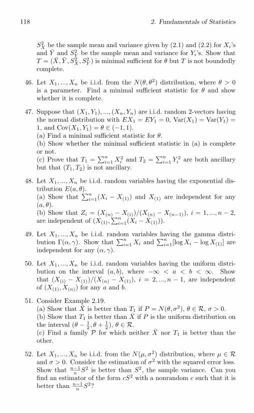
118 2. Fundamentals of Statistics
S2X be the sample mean and variance given by (2.1) and (2.2) for Xi’s
and Y and S2Y be the sample mean and variance for Yi’s. Show that
T = (X, Y , S2X , S2
Y ) is minimal sufficient for θ but T is not boundedlycomplete.
46. Let X1, ..., Xn be i.i.d. from the N(θ, θ2) distribution, where θ > 0is a parameter. Find a minimal sufficient statistic for θ and showwhether it is complete.
47. Suppose that (X1, Y1), ..., (Xn, Yn) are i.i.d. random 2-vectors havingthe normal distribution with EX1 = EY1 = 0, Var(X1) = Var(Y1) =1, and Cov(X1, Y1) = θ ∈ (−1, 1).(a) Find a minimal sufficient statistic for θ.(b) Show whether the minimal sufficient statistic in (a) is completeor not.(c) Prove that T1 =
∑ni=1 X
2i and T2 =
∑ni=1 Y
2i are both ancillary
but that (T1, T2) is not ancillary.
48. Let X1, ..., Xn be i.i.d. random variables having the exponential dis-tribution E(a, θ).(a) Show that
∑ni=1(Xi − X(1)) and X(1) are independent for any
(a, θ).(b) Show that Zi = (X(n) − X(i))/(X(n) − X(n−1)), i = 1, ..., n − 2,are independent of (X(1),
∑ni=1(Xi −X(1))).
49. Let X1, ..., Xn be i.i.d. random variables having the gamma distri-bution Γ(α, γ). Show that
∑ni=1 Xi and
∑ni=1[logXi − logX(1)] are
independent for any (α, γ).
50. Let X1, ..., Xn be i.i.d. random variables having the uniform distri-bution on the interval (a, b), where −∞ < a < b < ∞. Showthat (X(i) − X(1))/(X(n) − X(1)), i = 2, ..., n − 1, are independentof (X(1), X(n)) for any a and b.
51. Consider Example 2.19.(a) Show that X is better than T1 if P = N(θ, σ2), θ ∈ R, σ > 0.(b) Show that T1 is better than X if P is the uniform distribution onthe interval (θ − 1
2 , θ + 12 ), θ ∈ R.
(c) Find a family P for which neither X nor T1 is better than theother.
52. Let X1, ..., Xn be i.i.d. from the N(µ, σ2) distribution, where µ ∈ Rand σ > 0. Consider the estimation of σ2 with the squared error loss.Show that n−1
n S2 is better than S2, the sample variance. Can youfind an estimator of the form cS2 with a nonrandom c such that it isbetter than n−1
n S2?
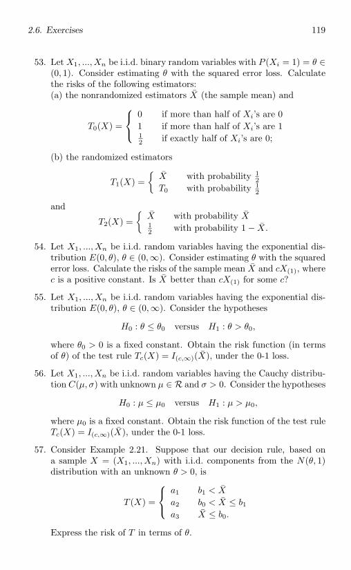
2.6. Exercises 119
53. Let X1, ..., Xn be i.i.d. binary random variables with P (Xi = 1) = θ ∈(0, 1). Consider estimating θ with the squared error loss. Calculatethe risks of the following estimators:(a) the nonrandomized estimators X (the sample mean) and
T0(X) =
⎧⎨⎩0 if more than half of Xi’s are 01 if more than half of Xi’s are 112 if exactly half of Xi’s are 0;
(b) the randomized estimators
T1(X) =
X with probability 12
T0 with probability 12
and
T2(X) =
X with probability X12 with probability 1 − X.
54. Let X1, ..., Xn be i.i.d. random variables having the exponential dis-tribution E(0, θ), θ ∈ (0,∞). Consider estimating θ with the squarederror loss. Calculate the risks of the sample mean X and cX(1), wherec is a positive constant. Is X better than cX(1) for some c?
55. Let X1, ..., Xn be i.i.d. random variables having the exponential dis-tribution E(0, θ), θ ∈ (0,∞). Consider the hypotheses
H0 : θ ≤ θ0 versus H1 : θ > θ0,
where θ0 > 0 is a fixed constant. Obtain the risk function (in termsof θ) of the test rule Tc(X) = I(c,∞)(X), under the 0-1 loss.
56. Let X1, ..., Xn be i.i.d. random variables having the Cauchy distribu-tion C(µ, σ) with unknown µ ∈ R and σ > 0. Consider the hypotheses
H0 : µ ≤ µ0 versus H1 : µ > µ0,
where µ0 is a fixed constant. Obtain the risk function of the test ruleTc(X) = I(c,∞)(X), under the 0-1 loss.
57. Consider Example 2.21. Suppose that our decision rule, based ona sample X = (X1, ..., Xn) with i.i.d. components from the N(θ, 1)distribution with an unknown θ > 0, is
T (X) =
⎧⎨⎩a1 b1 < X
a2 b0 < X ≤ b1a3 X ≤ b0.
Express the risk of T in terms of θ.
120 2. Fundamentals of Statistics
58. Consider an estimation problem with P = Pθ : θ ∈ Θ (a parametricfamily), A = Θ, and the squared error loss. If θ0 ∈ Θ satisfies thatPθ Pθ0 for any θ ∈ Θ, show that the estimator T ≡ θ0 is admissible.
59. Let be a class of decision rules. A subclass 0 ⊂ is called -complete if, for any T ∈ and T ∈ 0, there is a T0 ∈ 0 that isbetter than T , and is called -minimal complete if 0 is -completeand no proper subclass of 0 is -complete. Show that if a -minimalcomplete class exists, then it is exactly the class of -admissible rules.
60. Let X1, ..., Xn be i.i.d. random variables having a distribution P ∈ P.Assume that EX2
1 < ∞. Consider estimating µ = EX1 under thesquared error loss.(a) Show that any estimator of the form aX+b is inadmissible, whereX is the sample mean, a > 1 and b are constants.(b) Show that any estimator of the form X + b is inadmissible, whereb = 0 is a constant.
61. Consider an estimation problem with ϑ ∈ [a, b] ⊂ R, where a and bare known constants. Suppose that the action space is A ⊃ [a, b] andthe loss function is L(|ϑ−a|), where L(·) is an increasing function on[0,∞). Show that any decision rule T with P (T (X) ∈ [a, b]) > 0 forsome P ∈ P is inadmissible.
62. Show that the following functions of x are convex and discuss whetherthey are strictly convex.(a) |x− a|p, where p ≥ 1 and a ∈ R.(b) x−p, x ∈ (0,∞), where p > 0.(c) ecx, where c ∈ R.(d) − log x, x ∈ (0,∞).(e) ψ(φ(x)), x ∈ (a, b), where −∞ ≤ a < b ≤ ∞, φ is convex on (a, b),and ψ is convex and nondecreasing on the range of φ.(f) φ(x) =
∑ki=1 ciφi(xi), x = (x1, ..., xk) ∈
∏ki=1 Xi, where ci is a
positive constant and φi is convex on Xi, i = 1, ..., k.
63. Prove Theorem 2.5.
64. In Exercise 53, use Theorem 2.5 to find decision rules that are betterthan Tj , j = 0, 1, 2.
65. In Exercise 54, use Theorem 2.5 to find a decision rule better thancX(1).
66. Consider Example 2.22.(a) Show that there is no optimal rule if contains all possible esti-mators. (Hint: consider constant estimators.)
2.6. Exercises 121
(b) Find a 2-optimal rule if X1, ..., Xn are independent random vari-ables having a common mean µ and Var(Xi) = σ2/ai with known ai,i = 1, ..., n.(c) Find a 2-optimal rule if X1, ..., Xn are identically distributed butare correlated with a common correlation coefficient ρ.
67. Let T0(X) be an unbiased estimator of ϑ in an estimation problem.Show that any unbiased estimator of ϑ is of the form T (X) = T0(X)−U(X), where U(X) is an “unbiased estimator” of 0.
68. Let X be a discrete random variable with
P (X = −1) = p, P (X = k) = (1 − p)2pk, k = 0, 1, 2, ...,
where p ∈ (0, 1) is unknown.(a) Show that U(X) is an unbiased estimator of 0 if and only if U(k) =ak for all k = −1, 0, 1, 2, ... and some a.(b) Show that T0(X) = I0(X) is unbiased for ϑ = (1−p)2 and that,under the squared error loss, T0 is a -optimal rule, where is theclass of all unbiased estimators of ϑ.(c) Show that T0(X) = I−1(X) is unbiased for ϑ = p and that,under the squared error loss, there is no -optimal rule, where isthe class of all unbiased estimators of ϑ.
69. (Nonexistence of an unbiased estimator). Let X be a random variablehaving the binomial distribution Bi(p, n) with an unknown p ∈ (0, 1)and a known n. Consider the problem of estimating ϑ = p−1. Showthat there is no unbiased estimator of ϑ.
70. Let X1, ..., Xn be i.i.d. from the Poisson distribution P (θ) with anunknown θ > 0. Find the bias and mse of Tn = (1 − a/n)nX as anestimator of ϑ = e−aθ, where a = 0 is a known constant.
71. Consider a location family Pµ : µ ∈ Rk on Rk, where Pµ = P(µ,Ik)
given in (2.10). Let T = Ik, C = cl0 : c ∈ R, where l0 ∈ Rk isfixed, and L(P, a) = L(‖µ − a‖), where L(·) is a nonnegative Borelfunction on [0,∞). Show that the family is invariant and the decisionproblem is invariant with gc,A(a) = gc(a) = a+cl0. Find an invariantdecision rule.
72. Let X1, ..., Xn be i.i.d. from the N(µ, σ2) distribution with unknownµ ∈ R and σ2 > 0. Consider the scale transformation aX, a ∈ (0,∞).(a) For estimating σ2 under the loss function L(P, a) = (1 − a/σ2)2,show that the problem is invariant and that the sample variance S2
is invariant.
122 2. Fundamentals of Statistics
(b) For testing H0 : µ ≤ 0 versus H1 : µ > 0 under the loss
L(P, 0) =µ
σI(0,∞)(µ) and L(P, 1) =
|µ|σ
I(−∞,0](µ),
show that the problem is invariant and any test that is a function ofX/
√S2/n is invariant.
73. Let X1, ..., Xn be i.i.d. random variables having the c.d.f. F (x − θ),where F is symmetric about 0 and θ ∈ R is unknown.(a) Show that the c.d.f. of
∑ni=1 wiX(i) − θ is symmetric about 0,
where X(i) is the ith order statistic and wi’s are constants satisfyingwi = wn−i+1 and
∑ni=1 wi = 1.
(b) Show that∑n
i=1 wiX(i) in (a) is unbiased for θ if the mean of Fexists.(c) Show that
∑ni=1 wiX(i) is location invariant when
∑ni=1 wi = 1.
74. In Example 2.25, show that the conditional distribution of θ givenX = x is N(µ∗(x), c2) with µ∗(x) and c2 given by (2.28).
75. A median of a random variable Y (or its distribution) is any value msuch that P (Y ≤ m) ≥ 1
2 and P (Y ≥ m) ≥ 12 .
(a) Show that the set of medians is a closed interval [m0,m1].(b) Suppose that E|Y | < ∞. If c is not a median of Y , show thatE|Y − c| ≥ E|Y −m| for any median m of Y .(c) Let X be a sample from Pθ, where θ ∈ Θ ⊂ R. Consider theestimation of θ under the absolute error loss function |a − θ|. Let Πbe a given distribution on Θ with finite mean. Find the -Bayes rulew.r.t. Π, where is the class of all rules.
76. In Example 2.27, show that Y is still unbiased if sampling is withreplacement (see Exercise 2), and find the variance of Y .
77. Let X1, ..., Xn be i.i.d. random variables having the uniform distribu-tion U(0, θ), where θ > 0 is unknown. Calculate the bias and mse ofcX(n) as an estimator of θ, where c is a positive constant. Find a csuch that cX(n) is unbiased for θ.
78. Let X1, ..., Xn be i.i.d. from the N(µ, σ2) distribution with unknownµ ∈ R and σ2 > 0. Consider estimating ϑ = µ2. Calculate the biasand the mse of X2 as an estimator of ϑ. Find an unbiased estimator ofϑ based on the complete and sufficient statistic (X, S2) and compareits mse with that of X2.
79. Let X1, ..., Xn be i.i.d. from the N(µ, σ2) distribution with unknownµ ∈ R and σ2 > 0. To test the hypotheses
H0 : µ ≤ µ0 versus H1 : µ > µ0,
2.6. Exercises 123
where µ0 is a fixed constant, consider a test of the form Tc(X) =I(c,∞)(Tµ0), where Tµ0 = (X − µ0)/
√S2/n and c is a fixed constant.
(a) Find the size of Tc. (Hint: (X−µ0)/√S2/n has the t-distribution
tn−1.)(b) If α is a given level of significance, find a cα such that Tcα hassize α.(c) Compute the p-value for Tcα derived in (b).(d) Find a cα such that [X−cα
√S2/n, X+cα
√S2/n] is a confidence
interval for µ with confidence coefficient 1−α. What is the expectedinterval length?
80. In Exercise 55, calculate the size of Tc(X); find a cα such that Tcα
has size α, a given level of significance; and find the p-value for Tcα .
81. In Exercise 56, assume that σ is known. Calculate the size of Tc(X);find a cα such that Tcα has size α, a given level of significance; andfind the p-value for Tcα .
82. Let α ∈ (0, 1) be given and Tj,q(X) be the test given in Example 2.30.Show that there exist integer j and q ∈ (0, 1) such that the size ofTj,q is α.
83. Let X1, ..., Xn be i.i.d. from the exponential distribution E(a, θ) withunknown a ∈ R and θ > 0. Let α ∈ (0, 1) be given.(a) Using T1(X) =
∑ni=1(Xi −X(1)), construct a confidence interval
for θ with confidence coefficient 1 − α and find the expected intervallength.(b) Using T1(X) and T2(X) = X(1), construct a confidence intervalfor a with confidence coefficient 1 − α and find the expected intervallength.(c) Using the method in Example 2.32, construct a confidence set forthe two-dimensional parameter (a, θ) with confidence coefficient 1−α.
84. Suppose that X is a sample and a statistic T (X) has a distributionin a location family Pµ : µ ∈ R. Using T (X), derive a confidenceinterval for µ with level of significance 1−α and obtain the expectedinterval length. Show that if the c.d.f. of T (X) is continuous, then wecan always find a confidence interval for µ with confidence coefficient1 − α for any α ∈ (0, 1).
85. Let X = (X1, ..., Xn) be a sample from Pθ, where θ ∈ θ1, ..., θkwith a fixed integer k. Let Tn(X) be an estimator of θ with rangeθ1, ..., θk.(a) Show that Tn(X) is consistent if and only if Pθ(Tn(X) = θ) → 1.(b) Show that if Tn(X) is consistent, then it is an-consistent for anyan.
124 2. Fundamentals of Statistics
86. Let X1, ..., Xn be i.i.d. from the uniform distribution on (θ− 12 , θ+ 1
2 ),where θ ∈ R is unknown. Show that (X(1) + X(n))/2 is stronglyconsistent for θ and also consistent in mse.
87. Let X1, ..., Xn be i.i.d. from a population with the Lebesgue p.d.f.fθ(x) = 2−1(1 + θx)I(−1,1)(x), where θ ∈ (−1, 1) is an unknown pa-rameter. Find a consistent estimator of θ. Is your estimator
√n-
consistent?
88. Suppose that Tn is an unbiased estimator of ϑ such that for anyn, Var(Tn) < ∞ and Var(Tn) ≤ Var(Un) for any other unbiasedestimator of ϑ. Show that Tn is consistent in mse.
89. Consider the Bayes rule µ∗(X) in Example 2.25. Show that µ∗(X) isa strongly consistent,
√n-consistent, and L2-consistent estimator of
µ. What is the order of the bias of µ∗(X) as an estimator of µ?
90. Show that the estimator T0 of θ in Exercise 53 is inconsistent.
91. Let g1, g2,... be continuous functions on (a, b) ⊂ R such that gn(x) →g(x) uniformly for x in any closed subinterval of (a, b). Let Tn be aconsistent estimator of θ ∈ (a, b). Show that gn(Tn) is consistent forϑ = g(θ).
92. Let X1, ..., Xn be i.i.d. from P with unknown mean µ ∈ R and vari-ance σ2 > 0, and let g(µ) = 0 if µ = 0 and g(0) = 1. Find a consistentestimator of ϑ = g(µ).
93. Establish results for the smallest order statistic X(1) (based on i.i.d.random variables X1, ..., Xn) similar to those in Example 2.34.
94. (Consistency for finite population). In Example 2.27, show that Y →p
Y as n → N for any fixed N and population. Is Y still consistent ifsampling is with replacement?
95. Assume that Xi = θti + ei, i = 1, ..., n, where θ ∈ Θ is an unknownparameter, Θ is a closed subset of R, ei’s are i.i.d. on the interval[−τ, τ ] with some unknown τ > 0, and ti’s are fixed constants. Let
Tn = Sn(θn) = minγ∈Θ
Sn(γ),
whereSn(γ) = 2 max
i≤n|Xi − γti|/
√1 + γ2.
(a) Assume that supi |ti| < ∞ and supi ti − infi ti > 2τ . Show thatthe sequence θn, n = 1, 2, ... is bounded.(b) Let θn ∈ Θ, n = 1, 2, .... If θn → θ, show that
Sn(θn) − Sn(θ) = O(|θn − θ|).
2.6. Exercises 125
(c) Under the conditions in (a), show that Tn is a strongly consistentestimator of ϑ = minγ∈Θ S(γ), where S(γ) = limn→∞ Sn(γ) a.s.
96. Let X1, ..., Xn be i.i.d. from P with EX41 < ∞ and unknown mean
µ ∈ R and variance σ2 > 0. Consider the estimation of ϑ = µ2 andthe following three estimators: T1n = X2, T2n = X2 − S2/n, T3n =max(0, T2n), where X and S2 are the sample mean and variance.(a) Obtain n−1 order asymptotic biases for Tjn, j = 1, 2, 3.(b) Show that the regular amse’s of Tjn, j = 1, 2, 3, are the samewhen µ = 0 but may be different when µ = 0. Which estimator hasthe smallest limiting regular amse when µ = 0?
97. Let Tn be an estimator of ϑ satisfying√n(Tn − ϑ) →d N(0, σ2) for
some σ2 and limn→∞ nmseTn(P ) > σ2. Let Tcn = Tn + ξn(c)/√n,
where ξn(c) is a random variable independent of Tn, ξn(c) = c withprobability 1 − n−1 and ξn(c) = Z with probability n−1, c is a fixedconstant, and Z is a random variable having a Cauchy distribution.(a) Show that amseTn(P )/amseTcn(P ) → σ2/(c2 + σ2).(b) Show that mseTcn(P ) is not defined for any c and n.(c) Show that mseTn(P )/amseTcn(P ) converges to a constant largerthan 1 for some c.
98. Let X1, ..., Xn be i.i.d. according to N(µ, 1) with an unknown µ ∈ R.Let ϑ = P (X1 ≤ c) for a fixed constant c. Consider the followingestimators of ϑ: T1n = Fn(c), where Fn is the empirical c.d.f. definedin (2.31), and T2n = Φ(c− X), where Φ is the c.d.f. of N(0, 1).(a) Find an n−1 order asymptotic bias of T2n.(b) Find the asymptotic relative efficiency of T1n w.r.t. T2n.
99. Let X1, ..., Xn be i.i.d. from the N(0, σ2) distribution with an un-known σ > 0. Consider the estimation of ϑ = σ. Find the asymptoticrelative efficiency of
√π/2
∑ni=1 |Xi|/n w.r.t. (
∑ni=1 X
2i /n)1/2.
100. Show that if Eγ2n = amseTn(P ), limn→∞ a2
nEγ2n exists, and a2
nγ2n
is uniformly integrable, then Eγ2n = amseTn
(P ).
101. Prove Theorem 2.7.
102. Let X1, ..., Xn be i.i.d. with EXi = µ, Var(Xi) = 1, and EX4i < ∞.
Let T1n = n−1 ∑ni=1 X
2i − 1 and T2n = X2 − n−1 be estimators of
ϑ = µ2.(a) Find the asymptotic relative efficiency of T1n w.r.t. T2n.(b) Show that eT1n,T2n(P ) ≤ 1 if the c.d.f. of Xi − µ is symmetricabout 0.(c) Find a distribution P for which eT1n,T2n(P ) > 1.
126 2. Fundamentals of Statistics
103. Let X1, ..., Xn be i.i.d. binary random variables with unknown p =P (Xi = 1) ∈ (0, 1). Consider the estimation of p. Let a and b betwo positive constants. Find the asymptotic relative efficiency of theestimator (a + nX)/(a + b + n) w.r.t. X.
104. Let X1, ..., Xn be i.i.d. from the uniform distribution U(0, θ). Con-sider the following estimators of θ: T1n = (n + 1)X(n)/n and T2n =X(n). Find the biases bTjn
(θ), j = 1, 2, and eT1n,T2n(θ).
105. In Example 2.37, show that(a) (2.41) holds with α replaced by α(n) satisfying α(n) → 0 and√nα(n) → ∞;
(b) the limiting size of Tcα is 1 if P contains all possible populationson R.
106. Let X1, ..., Xn be i.i.d. with unknown mean µ ∈ R and varianceσ2 > 0. For testing H0 : µ ≤ µ0 versus H1 : µ > µ0, considerthe test Tcα obtained in Exercise 79(b).(a) Show that Tcα has asymptotic significance level α and is consis-tent.(b) Find a test that is Chernoff-consistent.
107. Consider the test Tj in Example 2.23. For each n, find a j = jn suchthat Tjn has asymptotic significance level α ∈ (0, 1).
108. Show that the test Tcα in Exercise 80 is consistent, but Tcα in Exercise81 is not consistent.
109. In Example 2.31, suppose that we drop the normality assumption butassume that µ = EXi and σ2 = Var(Xi) is known.(a) Show that the asymptotic significance level of the confidence in-terval [X − cα, X + cα], cα = σΦ−1(1 − α/2)/
√n is 1 − α.
(b) Show that the limiting confidence coefficient of the interval in (a)might be 0 if P contains all possible populations on R.
110. Let X1, ..., Xn be i.i.d. with unknown mean µ ∈ R and variance σ2 >0. Show that the confidence interval in Exercise 79(d) has asymptoticsignificance level 1 − α.
111. Let X1, ..., Xn be i.i.d. with unknown mean µ ∈ R and variance σ2 >0. Assume that EX4
1 < ∞. Using the sample variance S2, construct aconfidence interval for σ2 that has asymptotic significance level 1−α.
112. Consider the sample correlation coefficient T defined in Exercise 19.Construct a confidence interval for ρ that has asymptotic significancelevel 1 − α, assuming that (Yi, Zi) are normally distributed. (Hint:show that the asymptotic variance of T is (1 − ρ2)2.)
Chapter 3
Unbiased Estimation
Unbiased or asymptotically unbiased estimation plays an important role inpoint estimation theory. Unbiasedness of point estimators is defined in §2.3.In this chapter we discuss in detail how to derive unbiased estimators and,more importantly, how to find the best unbiased estimators in various situ-ations. Although an unbiased estimator (even the best unbiased estimatorif it exists) is not necessarily better than a slightly biased estimator in termsof their mse’s (see Exercise 52 in §2.6), unbiased estimators can be used as“building blocks” for the construction of better estimators. Furthermore,one may give up the exact unbiasedness, but cannot give up asymptoticunbiasedness since it is necessary for consistency (see §2.5). Properties andthe construction of asymptotically unbiased estimators are studied in thelast part of this chapter.
3.1 The UMVUE
Let X be a sample from an unknown population P ∈ P and ϑ be a real-valued parameter related to P . Recall that an estimator T (X) of ϑ isunbiased if E[T (X)] = ϑ for any P ∈ P. If there exists an unbiasedestimator of ϑ, then ϑ is called an estimable parameter.
Definition 3.1. An unbiased estimator T (X) of ϑ is called the uni-formly minimum variance unbiased estimator (UMVUE) if and only ifVar(T (X)) ≤ Var(U(X)) for any P ∈ P and any other unbiased estimatorU(X) of ϑ.
Since the mse of any unbiased estimator is its variance, a UMVUE is-optimal in mse with being the class of all unbiased estimators. One
127
128 3. Unbiased Estimation
can similarly define the uniformly minimum risk unbiased estimator in sta-tistical decision theory when we use an arbitrary loss instead of the squarederror loss that corresponds to the mse.
3.1.1 Sufficient and complete statistics
The derivation of a UMVUE is relatively simple if there exists a sufficientand complete statistic for P ∈ P.
Theorem 3.1. Suppose that there exists a sufficient and complete statisticT (X) for P ∈ P. If ϑ is estimable, then there is a unique unbiased estimatorof ϑ that is of the form h(T ) with a Borel function h. (Two estimators thatare equal a.s. P are treated as one estimator.) Furthermore, h(T ) is theunique UMVUE of ϑ.
This theorem is a consequence of Theorem 2.5(ii) (Rao-Blackwell’s theo-rem). One can easily extend this theorem to the case of uniformly minimumrisk unbiased estimator under any loss function L(P, a) which is strictly con-vex in a. The uniqueness of the UMVUE follows from the completeness ofT (X).
There are two typical ways to derive a UMVUE when a sufficient andcomplete statistic T is available. The first one is solving for h when thedistribution of T is available. The following are two typical examples.
Example 3.1. Let X1, ..., Xn be i.i.d. from the uniform distribution on(0, θ), θ > 0. Let ϑ = g(θ), where g is a differentiable function on (0,∞).Since the sufficient and complete statistic X(n) has the Lebesgue p.d.f.nθ−nxn−1I(0,θ)(x), an unbiased estimator h(X(n)) of ϑ must satisfy
θng(θ) = n
∫ θ
0h(x)xn−1dx for all θ > 0.
Assuming that h is continuous and differentiating both sizes of the previousequation lead to
nθn−1g(θ) + θng′(θ) = nh(θ)θn−1.
Hence, the UMVUE of ϑ is h(X(n)) = g(X(n)) + n−1X(n)g′(X(n)). In
particular, if ϑ = θ, then the UMVUE of θ is (1 + n−1)X(n).
Example 3.2. Let X1, ..., Xn be i.i.d. from the Poisson distribution P (θ)with an unknown θ > 0. Then T (X) =
∑ni=1 Xi is sufficient and complete
for θ > 0 and has the Poisson distribution P (nθ). Suppose that ϑ = g(θ),where g is a smooth function such that g(x) =
∑∞j=0 ajx
j , x > 0. An
3.1. The UMVUE 129
unbiased estimator h(T ) of ϑ must satisfy
∞∑t=0
h(t)nt
t!θt = enθg(θ)
=∞∑k=0
nk
k!θk
∞∑j=0
ajθj
=∞∑t=0
⎛⎝ ∑j,k:j+k=t
nkajk!
⎞⎠ θt
for any θ > 0. Thus, a comparison of coefficients in front of θt leads to
h(t) =t!nt
∑j,k:j+k=t
nkajk!
,
i.e., h(T ) is the UMVUE of ϑ. In particular, if ϑ = θr for some fixed integerr ≥ 1, then ar = 1 and ak = 0 if k = r and
h(t) =
0 t < r
t!nr(t−r)! t ≥ r.
The second method of deriving a UMVUE when there is a sufficient andcomplete statistic T (X) is conditioning on T , i.e., if U(X) is any unbiasedestimator of ϑ, then E[U(X)|T ] is the UMVUE of ϑ. To apply this method,we do not need the distribution of T , but need to work out the conditionalexpectation E[U(X)|T ]. From the uniqueness of the UMVUE, it does notmatter which U(X) is used and, thus, we should choose U(X) so as to makethe calculation of E[U(X)|T ] as easy as possible.
Example 3.3. Consider the estimation problem in Example 2.26, whereϑ = 1 − Fθ(t) and Fθ(x) = (1 − e−x/θ)I(0,∞)(x). Since X is sufficientand complete for θ > 0 and U(X) = 1 − Fn(t) is unbiased for ϑ, T (X) =E[U(X)|X] = E[1 − Fn(t)|X] is the UMVUE of ϑ. Since Xi’s are i.i.d.,
E[1 − Fn(t)|X] =1n
n∑i=1
P (Xi > t|X) = P (X1 > t|X).
If the conditional distribution of X1 given X is available, then we can cal-culate P (X1 > t|X) directly. But the following technique can be applied toavoid the derivation of conditional distributions. By Proposition 1.12(vii),
P (X1 > t|X = x) = P (X1/X > t/X|X = x) = P (X1/X > t/x|X = x).
130 3. Unbiased Estimation
By Basu’s theorem (Theorem 2.4), X1/X and X are independent. Hence
P (X1 > t|X = x) = P (X1/X > t/x).
To compute this probability, we need the distribution of
X1
/ n∑i=1
Xi = X1
/(X1 +
n∑i=2
Xi
).
Using the transformation technique discussed in §1.3.1 and the fact that∑ni=2 Xi is independent of X1 and has a gamma distribution, we obtain
that X1/∑n
i=1 Xi has the Lebesgue p.d.f. (n−1)(1−x)n−2I(0,1)(x). Hence
P (X1 > t|X = x) = (n− 1)∫ 1
t/(nx)(1 − x)n−2dx =
(1 − t
nx
)n−1
and the UMVUE of ϑ is T (X) = E[1 − Fn(t)|X] =(1 − t
nX
)n−1.
We now show more examples of applying these two methods to findUMVUE’s.
Example 3.4. Let X1, ..., Xn be i.i.d. from N(µ, σ2) with unknown µ ∈ Rand σ2 > 0. From Example 2.18, T = (X, S2) is sufficient and com-plete for θ = (µ, σ2) and X and (n − 1)S2/σ2 are independent and havethe N(µ, σ2/n) and chi-square distribution χ2
n−1, respectively. Using themethod of solving for h directly, we find that the UMVUE for µ is X; theUMVUE of µ2 is X2−S2/n; the UMVUE for σr with r > 1−n is kn−1,rS
r,where
kn,r =nr/2Γ(n/2)2r/2Γ
(n+r
2
)(exercise); and the UMVUE of µ/σ is kn−1,−1X/S, if n > 2.
Suppose that ϑ satisfies P (X1 ≤ ϑ) = p with a fixed p ∈ (0, 1). Let Φbe the c.d.f. of the standard normal distribution. Then ϑ = µ + σΦ−1(p)and its UMVUE is X + kn−1,1SΦ−1(p).
Let c be a fixed constant and ϑ = P (X1 ≤ c) = Φ(c−µσ
). We can
find the UMVUE of ϑ using the method of conditioning and the techniqueused in Example 3.3. Since I(−∞,c)(X1) is an unbiased estimator of ϑ, theUMVUE of ϑ is E[I(−∞,c)(X1)|T ] = P (X1 ≤ c|T ). By Basu’s theorem,the ancillary statistic Z(X) = (X1 − X)/S is independent of T = (X, S2).Then
P(X1 ≤ c|T = (x, s2)
)= P
(X1 − X
S≤ c− x
s
∣∣∣∣T = (x, s2))
= P
(Z ≤ c− x
s
).
3.1. The UMVUE 131
It can be shown that Z has the Lebesgue p.d.f.
f(z) =√nΓ
(n−1
2
)√π(n− 1)Γ
(n−2
2
) [1 − nz2
(n− 1)2
](n/2)−2
I(0,(n−1)/√n)(|z|) (3.1)
(exercise). Hence the UMVUE of ϑ is
P (X1 ≤ c|T ) =∫ (c−X)/S
−(n−1)/√n
f(z)dz (3.2)
with f given by (3.1).Suppose that we would like to estimate ϑ = 1
σΦ′ ( c−µσ
), the Lebesgue
p.d.f. of X1 evaluated at a fixed c, where Φ′ is the first-order derivativeof Φ. By (3.2), the conditional p.d.f. of X1 given X = x and S2 = s2 iss−1f
(x−xs
). Let fT be the joint p.d.f. of T = (X, S2). Then
ϑ =∫ ∫
1sf
(c− x
s
)fT (t)dt = E
[1Sf
(c− X
S
)].
Hence the UMVUE of ϑ is
1Sf
(c− X
S
).
Example 3.5. Let X1, ..., Xn be i.i.d. from a power series distribution (seeExercise 13 in §2.6), i.e.,
P (Xi = x) = γ(x)θx/c(θ), x = 0, 1, 2, ...
with a known function γ(x) ≥ 0 and an unknown parameter θ > 0. It turnsout that the joint distribution of X = (X1, ..., Xn) is in an exponential fam-ily with a sufficient and complete statistic T (X) =
∑ni=1 Xi. Furthermore,
the distribution of T is also in a power series family, i.e.,
P (T = t) = γn(t)θt/[c(θ)]n, t = 0, 1, 2, ...,
where γn(t) is the coefficient of θt in the power series expansion of [c(θ)]n
(exercise). This result can help us to find the UMVUE of ϑ = g(θ). Forexample, by comparing both sides of
∞∑t=0
h(t)γn(t)θt = [c(θ)]n−pθr,
we conclude that the UMVUE of θr/[c(θ)]p is
h(T ) =
0 T < rγn−p(T−r)
γn(T ) T ≥ r,

132 3. Unbiased Estimation
where r and p are nonnegative integers. In particular, the case of p = 1produces the UMVUE γ(r)h(T ) of the probability P (X1 = r) = γ(r)θr/c(θ)for any nonnegative integer r.
Example 3.6. Let X1, ..., Xn be i.i.d. from an unknown population P in anonparametric family P. We have discussed in §2.2 that in many cases thevector of order statistics, T = (X(1), ..., X(n)), is sufficient and complete forP ∈ P. Note that an estimator ϕ(X1, ..., Xn) is a function of T if and only ifthe function ϕ is symmetric in its n arguments. Hence, if T is sufficient andcomplete, then a symmetric unbiased estimator of any estimable ϑ is theUMVUE. For example, X is the UMVUE of ϑ = EX1; S2 is the UMVUEof Var(X1); n−1 ∑n
i=1 X2i − S2 is the UMVUE of (EX1)2; and Fn(t) is the
UMVUE of P (X1 ≤ t) for any fixed t.Note that these conclusions are not true if T is not sufficient and com-
plete for P ∈ P. For example, if P contains all symmetric distributionshaving Lebesgue p.d.f.’s and finite means, then there is no UMVUE forϑ = EX1 (exercise).
More discussions of UMVUE’s in nonparametric problems are providedin §3.2.
3.1.2 A necessary and sufficient condition
When a complete and sufficient statistic is not available, it is usually verydifficult to derive a UMVUE. In some cases, the following result can beapplied, if we have enough knowledge about unbiased estimators of 0.
Theorem 3.2. Let U be the set of all unbiased estimators of 0 with finitevariances and T be an unbiased estimator of ϑ with E(T 2) < ∞.(i) A necessary and sufficient condition for T (X) to be a UMVUE of ϑ isthat E[T (X)U(X)] = 0 for any U ∈ U and any P ∈ P.(ii) Suppose that T = h(T ), where T is a sufficient statistic for P ∈ P andh is a Borel function. Let UT be the subset of U containing Borel functionsof T . Then a necessary and sufficient condition for T to be a UMVUE of ϑis that E[T (X)U(X)] = 0 for any U ∈ UT and any P ∈ P.Proof. (i) Suppose that T is a UMVUE of ϑ. Then Tc = T + cU , whereU ∈ U and c is a fixed constant, is also unbiased for ϑ and, thus,
Var(Tc) ≥ Var(T ) c ∈ R, P ∈ P,
which is the same as
c2Var(U) + 2cCov(T,U) ≥ 0 c ∈ R, P ∈ P.
This is impossible unless Cov(T,U) = E(TU) = 0 for any P ∈ P.
3.1. The UMVUE 133
Suppose now E(TU) = 0 for any U ∈ U and P ∈ P. Let T0 be anotherunbiased estimator of ϑ with Var(T0) < ∞. Then T − T0 ∈ U and, hence,
E[T (T − T0)] = 0 P ∈ P,
which with the fact that ET = ET0 implies that
Var(T ) = Cov(T, T0) P ∈ P.
By inequality (1.34), [Cov(T, T0)]2 ≤ Var(T )Var(T0). Hence Var(T ) ≤Var(T0) for any P ∈ P.(ii) It suffices to show that E(TU) = 0 for any U ∈ UT and P ∈ P impliesthat E(TU) = 0 for any U ∈ U and P ∈ P. Let U ∈ U . Then E(U |T ) ∈ UT
and the result follows from the fact that T = h(T ) and
E(TU) = E[E(TU |T )] = E[E(h(T )U |T )] = E[h(T )E(U |T )].
Theorem 3.2 can be used to find a UMVUE, to check whether a partic-ular estimator is a UMVUE, and to show the nonexistence of any UMVUE.If there is a sufficient statistic, then by Rao-Blackwell’s theorem, we onlyneed to focus on functions of the sufficient statistic and, hence, Theorem3.2(ii) is more convenient to use.
Example 3.7. Let X1, ..., Xn be i.i.d. from the uniform distribution onthe interval (0, θ). In Example 3.1, (1 + n−1)X(n) is shown to be theUMVUE for θ when the parameter space is Θ = (0,∞). Suppose now thatΘ = [1,∞). Then X(n) is not complete, although it is still sufficient for θ.Thus, Theorem 3.1 does not apply. We now illustrate how to use Theorem3.2(ii) to find a UMVUE of θ. Let U(X(n)) be an unbiased estimator of 0.Since X(n) has the Lebesgue p.d.f. nθ−nxn−1I(0,θ)(x),
0 =∫ 1
0U(x)xn−1dx +
∫ θ
1U(x)xn−1dx
for all θ ≥ 1. This implies that U(x) = 0 a.e. Lebesgue measure on [1,∞)and ∫ 1
0U(x)xn−1dx = 0.
Consider T = h(X(n)). To have E(TU) = 0, we must have∫ 1
0h(x)U(x)xn−1dx = 0.
Thus, we may consider the following function:
h(x) =
c 0 ≤ x ≤ 1bx x > 1,
134 3. Unbiased Estimation
where c and b are some constants. From the previous discussion,
E[h(X(n))U(X(n))] = 0, θ ≥ 1.
Since E[h(X(n))] = θ, we obtain that
θ = cP (X(n) ≤ 1) + bE[X(n)I(1,∞)(X(n))]
= cθ−n + [bn/(n + 1)](θ − θ−n).
Thus, c = 1 and b = (n + 1)/n. The UMVUE of θ is then
T =
1 0 ≤ X(n) ≤ 1(1 + n−1)X(n) X(n) > 1.
This estimator is better than (1 + n−1)X(n) which is the UMVUE whenΘ = (0,∞) and does not make use of the information about θ ≥ 1.
Example 3.8. Let X be a sample (of size 1) from the uniform distributionU(θ − 1
2 , θ + 12 ), θ ∈ R. We now apply Theorem 3.2 to show that there is
no UMVUE of ϑ = g(θ) for any nonconstant continuous g. Note that anunbiased estimator U(X) of 0 must satisfy∫ θ+ 1
2
θ− 12
U(x)dx = 0 θ ∈ R
and, hence, U(x) = U(x + 1) a.e. m, where m is the Lebesgue measureon R. If T is a UMVUE, then T (X)U(X) is unbiased for 0 and, hence,T (x)U(x) = T (x + 1)U(x + 1) a.e. m, which implies that T (x) = T (x + 1)a.e. m. If T is unbiased for g(θ), then
g(θ) =∫ θ+ 1
2
θ− 12
T (x)dx θ ∈ R,
which implies that
g′(θ) = T(θ + 1
2
)− T
(θ − 1
2
)= 0 a.e. m
As a consequence of Theorem 3.2, we have the following useful result.
Corollary 3.1. (i) Let Tj be a UMVUE of ϑj , j = 1, ..., k, where k is afixed positive integer. Then
∑kj=1 cjTj is a UMVUE of ϑ =
∑kj=1 cjϑj for
any constants c1, ..., ck.(ii) Let T1 and T2 be two UMVUE’s of ϑ. Then T1 = T2 a.s. P for anyP ∈ P.
3.1. The UMVUE 135
3.1.3 Information inequality
Suppose that we have a lower bound for the variances of all unbiased esti-mators of ϑ and that there is an unbiased estimator T of ϑ whose varianceis always the same as the lower bound. Then T is a UMVUE of ϑ. Al-though this is not an effective way to find UMVUE’s (compared with themethods introduced in §3.1.1 and §3.1.2), it provides a way of assessingthe performance of UMVUE’s. The following result provides such a lowerbound in some cases.
Theorem 3.3 (The Cramer-Rao lower bound). Let X = (X1, ..., Xn)be a sample from P ∈ P = Pθ : θ ∈ Θ, where Θ is an open set inRk. Suppose that T (X) is an estimator with E[T (X)] = g(θ) being adifferentiable function of θ; the joint distribution of X has a p.d.f. fθ w.r.t.a measure ν for all θ ∈ Θ; and fθ is differentiable as a function of θ andsatisfies
∂
∂θ
∫h(x)fθ(x)dν =
∫h(x)
∂
∂θfθ(x)dν, θ ∈ Θ, (3.3)
for h(x) ≡ 1 and h(x) = T (x). Then
Var(T (X)) ≥ ∂∂θg(θ)[I(θ)]
−1[
∂∂θg(θ)
]τ, (3.4)
where
I(θ) = E
[∂
∂θlog fθ(X)
]τ [∂
∂θlog fθ(X)
](3.5)
is assumed to be positive definite for any θ ∈ Θ.Proof. We prove the univariate case (k = 1) only. The proof for themultivariate case (k > 1) is left to the reader. When k = 1, (3.4) reducesto
Var(T (X)) ≥ [g′(θ)]2
E[
∂∂θ log fθ(X)
]2 . (3.6)
From inequality (1.34), we only need to show that
E
[∂
∂θlog fθ(X)
]2
= Var(
∂
∂θlog fθ(X)
)and
g′(θ) = Cov(T (X),
∂
∂θlog fθ(X)
).
These two results are consequences of condition (3.3).
The k × k matrix I(θ) in (3.5) is called the Fisher information matrix.The greater I(θ) is, the easier it is to distinguish θ from neighboring values
136 3. Unbiased Estimation
and, therefore, the more accurately θ can be estimated. In fact, if theequality in (3.6) holds for an unbiased estimator T (X) of g(θ) (which isthen a UMVUE), then the greater I(θ) is, the smaller Var(T (X)) is. Thus,I(θ) is the information that X contains about the unknown parameter θ.The inequalities in (3.4) and (3.6) are called information inequalities.
The following result is helpful in finding the Fisher information matrix.
Proposition 3.1. (i) Let X and Y be independent with the Fisher informa-tion matrices IX(θ) and IY (θ), respectively. Then the Fisher informationabout θ contained in (X,Y ) is IX(θ) + IY (θ). In particular, if X1, ..., Xn
are i.i.d. and I(θ) is the Fisher information about θ contained in a singleXi, then the Fisher information about θ contained in X1, ..., Xn is nI(θ).(ii) Suppose that X has the p.d.f. fθ which is twice differentiable in θ andthat (3.3) holds with h(x) ≡ 1 and fθ replaced by ∂fθ/∂θ. Then
I(θ) = −E
[∂2
∂θ∂θτlog fθ(X)
]. (3.7)
Proof. Result (i) follows from the independence of X and Y and thedefinition of the Fisher information. Result (ii) follows from the equality
∂2
∂θ∂θτlog fθ(X) =
∂2
∂θ∂θτ fθ(X)fθ(X)
−[∂
∂θlog fθ(X)
]τ [∂
∂θlog fθ(X)
].
The following example provides a formula for the Fisher informationmatrix for many parametric families with a two-dimensional parameter θ.
Example 3.9. Let X1, ..., Xn be i.i.d. with the Lebesgue p.d.f. 1σf
(x−µσ
),
where f(x) > 0 and f ′(x) exists for all x ∈ R, µ ∈ R, and σ > 0 (alocation-scale family). Let θ = (µ, σ). Then the Fisher information aboutθ contained in X1, ..., Xn is (exercise)
I(θ) =n
σ2
⎛⎜⎝∫ [f ′(x)]2
f(x) dx∫x [f ′(x)]2
f(x) dx
∫x [f ′(x)]2
f(x) dx∫ [xf ′(x)+f(x)]2
f(x) dx
⎞⎟⎠ .
Note that I(θ) depends on the particular parameterization. If θ = ψ(η)and ψ is differentiable, then the Fisher information that X contains aboutη is
∂∂ηψ(η)I(ψ(η))
[∂∂ηψ(η)
]τ.
However, it is easy to see that the Cramer-Rao lower bound in (3.4) or (3.6)is not affected by any one-to-one reparameterization.
3.1. The UMVUE 137
If we use inequality (3.4) or (3.6) to find a UMVUE T (X), then weobtain a formula for Var(T (X)) at the same time. On the other hand, theCramer-Rao lower bound in (3.4) or (3.6) is typically not sharp. Undersome regularity conditions, the Cramer-Rao lower bound is attained if andonly if fθ is in an exponential family; see Propositions 3.2 and 3.3 andthe discussion in Lehmann (1983, p. 123). Some improved informationinequalities are available (see, e.g., Lehmann (1983, Sections 2.6 and 2.7)).
Proposition 3.2. Suppose that the distribution of X is from an exponen-tial family fθ : θ ∈ Θ, i.e., the p.d.f. of X w.r.t. a measure ν is
fθ(x) = expT (x)[η(θ)]τ − ξ(θ)
c(x) (3.8)
(see §2.1.3), where Θ is an open subset of Rk.(i) The regularity condition (3.3) is satisfied for any h with E|h(X)| < ∞and (3.7) holds.(ii) If I(η) is the Fisher information matrix for the natural parameter η,then the variance-covariance matrix Var(T ) = I(η).(iii) If I(ϑ) is the Fisher information matrix for the parameter ϑ = E[T (X)],then Var(T ) = [I(ϑ)]−1.Proof. (i) This is a direct consequence of Theorem 2.1.(ii) From (2.6), the p.d.f. under the natural parameter η is
fη(x) = exp T (x)ητ − ζ(η) c(x).
From Proposition 1.10 and Theorem 2.1, E[T (X)] = ∂∂η ζ(η). The result
follows from∂∂η log fη(x) = T (x) − ∂
∂η ζ(η).
(iii) Since ϑ = E[T (X)] = ∂∂η ζ(η),
I(η) = ∂ϑ∂η I(ϑ)∂ϑ
τ
∂η = ∂2
∂η∂ητ ζ(η)I(ϑ)[
∂2
∂η∂ητ ζ(η)]τ
.
By Proposition 1.10, Theorem 2.1, and the result in (ii), ∂2
∂η∂ητ ζ(η) =Var(T ) = I(η). Hence
I(ϑ) = [I(η)]−1I(η)[I(η)]−1 = [I(η)]−1 = [Var(T )]−1.
A direct consequence of Proposition 3.2(ii) is that the variance of anylinear function of T in (3.8) attains the Cramer-Rao lower bound. Thefollowing result gives a necessary condition for Var(U(X)) of an estimatorU(X) to attain the Cramer-Rao lower bound.
138 3. Unbiased Estimation
Proposition 3.3. Let U(X) be an estimator of g(θ) = E[U(X)]. Assumethat the conditions in Theorem 3.3 hold for U(x) and that Θ ⊂ R.(i) If Var(U(X)) attains the Cramer-Rao lower bound in (3.6), then
a(θ)[U(X) − g(θ)] = g′(θ)∂
∂θlog fθ(X) a.s. fθ
for some function a(θ), θ ∈ Θ.(ii) Let fθ and T be given by (3.8). If Var(U(X)) attains the Cramer-Raolower bound, then U(X) is a linear function of T (X) a.s. fθ, θ ∈ Θ.
Example 3.10. Let X1, ..., Xn be i.i.d. from the N(µ, σ2) distribution withan unknown µ ∈ R and a known σ2. Let fµ be the joint distribution ofX = (X1, ..., Xn). Then
∂∂µ log fµ(X) =
n∑i=1
(Xi − µ)/σ2.
Thus, I(µ) = n/σ2. It is obvious that Var(X) attains the Cramer-Rao lowerbound in (3.6). Consider now the estimation of ϑ = µ2. Since EX2 =µ2 + σ2/n, the UMVUE of ϑ is h(X) = X2 − σ2/n. A straightforwardcalculation shows that
Var(h(X)) =4µ2σ2
n+
2σ4
n2 .
On the other hand, the Cramer-Rao lower bound in this case is 4µ2σ2/n.Hence Var(h(X)) does not attain the Cramer-Rao lower bound. The dif-ference is 2σ4/n2.
Condition (3.3) is a key regularity condition for the results in Theorem3.3 and Proposition 3.3. If fθ is not in an exponential family, then (3.3) hasto be checked. Typically, it does not hold if the set x : fθ(x) > 0 dependson θ (Exercise 32). More discussions can be found in Pitman (1979).
3.1.4 Asymptotic properties of UMVUE’s
UMVUE’s are typically consistent (see Exercise 88 in §2.6). If there is anunbiased estimator of ϑ whose mse is of the order a−2
n , where an is asequence of positive numbers diverging to ∞, then the UMVUE of ϑ (ifit exists) has a mse of order a−2
n and is an-consistent. For instance, inExample 3.3, the mse of U(X) = 1− Fn(t) is Fθ(t)[1− Fθ(t)]/n; hence theUMVUE T (X) is
√n-consistent and its mse is of the order n−1.
UMVUE’s are exactly unbiased so that there is no need to discuss theirasymptotic biases. Their variances (or mse’s) are finite, but amse’s can
3.1. The UMVUE 139
be used to approximate their mse’s if the exact forms of these mse’s aredifficult to obtain. In many cases, although the variance of a UMVUE Tn
does not attain the Cramer-Rao lower bound, the limit of the ratio of theamse (or mse) of Tn over the Cramer-Rao lower bound (if it is not 0) is 1.For instance, in Example 3.10,
Var(X2 − σ2/n)the Cramer-Rao lower bound
= 1 +σ2
2µ2n→ 1
if µ = 0. In general, under the conditions in Theorem 3.3, if Tn(X) isunbiased for g(θ) and if for any θ ∈ Θ,
Tn(X) − g(θ) = ∂∂θg(θ)[I(θ)]
−1[
∂∂θ log fθ(X)
]τ[1 + op(1)] a.s. fθ, (3.9)
thenamseTn
(θ) = the Cramer-Rao lower bound (3.10)whenever the Cramer-Rao lower bound is not 0. Note that the case of zeroCramer-Rao lower bound is not of interest since a zero lower bound doesnot provide any information on the performance of estimators.
Consider the UMVUE Tn =(1 − t
nX
)n−1 of e−t/θ in Example 3.3.Using the fact that
log(1 − x) = −∞∑j=1
xj
j, |x| ≤ 1,
we obtain thatTn − e−t/X = Op
(n−1) .
Using Taylor’s expansion, we obtain that
e−t/X − e−t/θ = g′(θ)(X − θ)[1 + op(1)],
where g(θ) = e−t/θ. On the other hand,
[I(θ)]−1 ∂∂θ log fθ(X) = X − θ.
Hence (3.9) and (3.10) hold. Note that the exact variance of Tn is noteasy to obtain. In this example, it can be shown that n[Tn − g(θ)]2 isuniformly integrable and, therefore,
limn→∞
nVar(Tn) = limn→∞
n[amseTn(θ)]
= limn→∞
n[g′(θ)]2[I(θ)]−1
=t2e−2t/θ
θ2 .
It is shown in Chapter 4 that if (3.10) holds, then Tn is asymptoticallyoptimal in some sense. Hence UMVUE’s satisfying (3.9), which is oftentrue, are asymptotically optimal, although they may be improved in termsof the exact mse’s.
140 3. Unbiased Estimation
3.2 U-Statistics
Let X1, ..., Xn be i.i.d. from an unknown population P in a nonparametricfamily P. In Example 3.6 we argued that if the vector of order statistic issufficient and complete for P ∈ P, then a symmetric unbiased estimator ofany estimable ϑ is the UMVUE of ϑ. In a large class of problems parametersto be estimated are of the form
ϑ = E[h(X1, ..., Xm)]
with a positive integer m and a Borel function h which is symmetric andsatisfies E|h(X1, ..., Xm)| < ∞ for any P ∈ P. It is easy to see that asymmetric unbiased estimator of ϑ is
Un =(n
m
)−1 ∑c
h(Xi1 , ..., Xim), (3.11)
where∑
c denotes the summation over the(nm
)combinations of m distinct
elements i1, ..., im from 1, ..., n.
Definition 3.2. The statistic Un in (3.11) is called a U -statistic with kernelh of order m.
3.2.1 Some examples
The use of U-statistics is an effective way of obtaining unbiased estimators.In nonparametric problems, U-statistics are often UMVUE’s, whereas inparametric problems, U-statistics can be used as initial estimators to derivemore efficient estimators.
If m = 1, Un in (3.11) is simply a type of sample mean. Examplesinclude the empirical c.d.f. (2.31) evaluated at a particular t and the samplemoments n−1 ∑n
i=1 Xki for a positive integer k. We now consider some
examples with m > 1.Consider the estimation of ϑ = µm, where µ = EX1 and m is a positive
integer. Using h(x1, ..., xm) = x1 · · ·xm, we obtain the following U-statisticunbiased for ϑ = µm:
Un =(n
m
)−1 ∑c
Xi1 · · ·Xim . (3.12)
Consider next the estimation of ϑ = σ2 = Var(X1). Since
σ2 = [Var(X1) + Var(X2)]/2 = E[(X1 −X2)2/2],
3.2. U-Statistics 141
we obtain the following U-statistic with kernel h(x1, x2) = (x1 − x2)2/2:
Un =2
n(n− 1)
∑1≤i<j≤n
(Xi −Xj)2
2=
1n− 1
(n∑
i=1
X2i − nX2
)= S2,
which is the sample variance in (2.2).In some cases we would like to estimate ϑ = E|X1 −X2|, a measure of
concentration. Using kernel h(x1, x2) = |x1 − x2|, we obtain the followingU-statistic unbiased for ϑ = E|X1 −X2|:
Un =2
n(n− 1)
∑1≤i<j≤n
|Xi −Xj |,
which is known as Gini’s mean difference.Let ϑ = P (X1 + X2 ≤ 0). Using kernel h(x1, x2) = I(−∞,0)(x1 + x2),
we obtain the following U-statistic unbiased for ϑ:
Un =2
n(n− 1)
∑1≤i<j≤n
I(−∞,0)(Xi + Xj),
which is known as the one-sample Wilcoxon statistic.Let Tn = Tn(X1, ..., Xn) be a given statistic and let r and d be two
positive integers such that r + d = n. For any s = i1, ..., ir ⊂ 1, ..., n,define
Tr,s = Tr(Xi1 , ..., Xir ),
which is the statistic Tn computed after Xi, i ∈ s, are deleted from theoriginal sample. Let
Un =(n
r
)−1 ∑c
rd (Tr,s − Tn)2. (3.13)
Then Un is a U-statistic with kernel
hn(x1, ..., xr) = rd [Tr(x1, ..., xr) − Tn(x1, ..., xn)].
Unlike the kernels in the previous examples, the kernel in this exampledepends on n. The order of the kernel, r, may also depend on n. Thestatistic Un in (3.13) is known as the delete-d jackknife variance estimatorfor Tn (see, e.g., Shao and Tu (1995)), since it is often true that
E[hn(X1, ..., Xr)] ≈ Var(Tn).
It can be shown that if Tn = X, then nUn in (3.13) is exactly the same asthe sample variance S2 (exercise).
142 3. Unbiased Estimation
3.2.2 Variances of U-statistics
If E[h(X1, ..., Xm)]2 < ∞, then the variance of Un in (3.11) with kernelh has an explicit form. To derive Var(Un), we need some notation. Fork = 1, ...,m, let
hk(x1, ..., xk) = E[h(X1, ..., Xm)|X1 = x1, ..., Xk = xk]= E[h(x1, ..., xk, Xk+1, ..., Xm)].
It can be shown that
hk(x1, ..., xk) = E[hk+1(x1, ..., xk, Xk+1)]. (3.14)
Definehk = hk − E[h(X1, ..., Xm)]. (3.15)
Then, for any Un defined by (3.11),
Un − E(Un) =(n
m
)−1 ∑c
hm(Xi1 , ..., Xim). (3.16)
Theorem 3.4 (Hoeffding’s theorem). For a U-statistic Un given by (3.11)with E[h(X1, ..., Xm)]2 < ∞,
Var(Un) =(n
m
)−1 m∑k=1
(m
k
)(n−m
m− k
)ζk,
whereζk = Var(hk(X1, ..., Xk)).
Proof. Consider two sets i1, ..., im and j1, ..., jm of m distinct integersfrom 1, ..., n with exactly k integers in common. The number of distinctchoices of two such sets is
(nm
)(mk
)(n−mm−k
). By the symmetry of hm and
independence of X1, ..., Xn,
E[hm(Xi1 , ..., Xim)hm(Xj1 , ..., Xjm)] = ζk (3.17)
for k = 1, ...,m (exercise). Then, by (3.16),
Var(Un) =(n
m
)−2 ∑c
∑c
E[hm(Xi1 , ..., Xim)hm(Xj1 , ..., Xjm)]
=(n
m
)−2 m∑k=1
(n
m
)(m
k
)(n−m
m− k
)ζk.
This proves the result.
3.2. U-Statistics 143
Corollary 3.2. Under the condition of Theorem 3.4,(i) m2
n ζ1 ≤ Var(Un) ≤ mn ζm;
(ii) (n + 1)Var(Un+1) ≤ nVar(Un) for any n > m;(iii) For any fixed m and k = 1, ...,m, if ζj = 0 for j < k and ζk > 0, then
Var(Un) =k!(mk
)2ζk
nk+ O
(1
nk+1
).
It follows from Corollary 3.2 that a U-statistic Un as an estimator of itsmean is consistent in mse (under the finite second moment assumption onh). In fact, for any fixed m, if ζj = 0 for j < k and ζk > 0, then the mse ofUn is of the order n−k and, therefore, Un is nk/2-consistent.
Example 3.11. Consider first h(x1, x2) = x1x2 which leads to a U-statisticunbiased for µ2, µ = EX1. Note that h1(x1) = µx1, h1(x1) = µ(x1 − µ),ζ1 = E[h1(X1)]2 = µ2Var(X1) = µ2σ2, h2(x1, x2) = x1x2 − µ2, and ζ2 =Var(X1X2) = E(X1X2)2 − µ4 = (µ2 + σ2)2 − µ4. By Theorem 3.4, forUn =
(n2
)−1 ∑1≤i<j≤n XiXj ,
Var(Un) =(n
2
)−1 [(21
)(n− 2
1
)ζ1 +
(22
)(n− 2
0
)ζ2
]=
2n(n− 1)
[2(n− 2)µ2σ2 + (µ2 + σ2)2 − µ4]
=4µ2σ2
n+
2σ4
n(n− 1).
Comparing Un with X2 − σ2/n in Example 3.10, which is the UMVUEunder the normality and known σ2 assumption, we find that
Var(Un) − Var(X2 − σ2/n) =2σ4
n2(n− 1).
Next, consider h(x1, x2) = I(−∞,0)(x1 + x2) which leads to the one-sample Wilcoxon statistic. Note that h1(x1) = P (x1 + X2 ≤ 0) = F (−x1),where F is the c.d.f. of P . Then ζ1 = Var(F (−X1)). Let ϑ = E[h(X1, X2)].Then ζ2 = Var(h(X1, X2)) = ϑ(1−ϑ). Hence, for Un being the one-sampleWilcoxon statistic,
Var(Un) =2
n(n− 1)[2(n− 2)ζ1 + ϑ(1 − ϑ)] .
If F is continuous and symmetric about 0, then ζ1 can be simplified as
ζ1 = Var(F (−X1)) = Var(1 − F (X1)) = Var(F (X1)) = 112 ,
144 3. Unbiased Estimation
since F (X1) has the uniform distribution on [0, 1].Finally, consider h(x1, x2) = |x1 − x2|, which leads to Gini’s mean dif-
ference. Note that
h1(x1) = E|x1 −X2| =∫
|x1 − y|dP (y),
and
ζ1 = Var(h1(X1)) =∫ [∫
|x− y|dP (y)]2
dP (x) − ϑ2,
where ϑ = E|X1 −X2|.
3.2.3 The projection method
Since P is nonparametric, the exact distribution of any U-statistic is hardto derive. In this section we study asymptotic distributions of U-statistics,using the method of projection.
Definition 3.3. Let Tn be a given statistic based on X1, ..., Xn. Theprojection of Tn on kn random elements Y1, ..., Ykn is defined to be
Tn = E(Tn) +kn∑i=1
[E(Tn|Yi) − E(Tn)].
Let ψn(Xi) = E(Tn|Xi). If Tn is symmetric (as a function of X1, ..., Xn),then ψn(X1), ..., ψn(Xn) are i.i.d. with mean E[ψn(Xi)] = E[E(Tn|Xi)] =E(Tn). If E(T 2
n) < ∞ and Var(ψn(Xi)) > 0, then
1√nVar(ψn(X1))
n∑i=1
[ψn(Xi) − E(Tn)] →d N(0, 1) (3.18)
by the CLT. Let Tn be the projection of Tn on X1, ..., Xn. Then
Tn − Tn = Tn − E(Tn) −n∑
i=1
[ψn(Xi) − E(Tn)]. (3.19)
If we can show that Tn − Tn has a negligible order of magnitude, thenwe can derive the asymptotic distribution of Tn by using (3.18)-(3.19) andSlutsky’s theorem. The order of magnitude of Tn− Tn can be obtained withthe help of the following lemma.
Lemma 3.1. Let Tn be a symmetric statistic with Var(Tn) < ∞ for everyn and Tn be the projection of Tn on X1, ..., Xn. Then E(Tn) = E(Tn) and
E(Tn − Tn)2 = Var(Tn) − Var(Tn).
3.2. U-Statistics 145
Proof. Since E(Tn) = E(Tn),
E(Tn − Tn)2 = Var(Tn) + Var(Tn) − 2Cov(Tn, Tn).
From Definition 3.3 with Yi = Xi,
Var(Tn) = nVar(E(Tn|Xi)).
The result follows from
Cov(Tn, Tn) = E(TnTn) − [E(Tn)]2
= nE[TnE(Tn|Xi)] − n[E(Tn)]2
= nEE[TnE(Tn|Xi)|Xi] − n[E(Tn)]2
= nE[E(Tn|Xi)]2 − n[E(Tn)]2
= nVar(E(Tn|Xi))= Var(Tn).
This method of deriving the asymptotic distribution of Tn is known asthe method of projection and is particularly effective for U-statistics. Fora U-statistic Un given by (3.11), one can show (exercise) that
Un = E(Un) +m
n
n∑i=1
h1(Xi), (3.20)
where Un is the projection of Un on X1, ..., Xn and h1 is defined by (3.15).Hence
Var(Un) = m2ζ1/n
and, by Corollary 3.2 and Lemma 3.1,
E(Un − Un)2 = O(n−2).
If ζ1 > 0, then (3.18) holds with ψn(Xi) = mh1(Xi), which leads to theresult in Theorem 3.5(i) stated later.
If ζ1 = 0, then h1 ≡ 0 and we have to use another projection of Un.Suppose that ζ1 = · · · = ζk−1 = 0 and ζk > 0 for an integer k > 1. Considerthe projection Ukn of Un on Xi1 , ..., Xik, 1 ≤ i1 < · · · < ik ≤ n. We canestablish a result similar to that in Lemma 3.1 (exercise) and show that
E(Un − Un)2 = O(n−(k+1)).
Also, see Serfling (1980, §5.3.4).With these results, we obtain the following theorem.
146 3. Unbiased Estimation
Theorem 3.5. Let Un be given by (3.11) with E[h(X1, ..., Xm)]2 < ∞.(i) If ζ1 > 0, then
√n[Un − E(Un)] →d N(0,m2ζ1).
(ii) If ζ1 = 0 but ζ2 > 0, then
n[Un − E(Un)] →dm(m− 1)
2
∞∑j=1
λj(χ21j − 1), (3.21)
where χ21j ’s are i.i.d. random variables having the chi-square distribution χ2
1and λj ’s are some constants (which may depend on P ) satisfying
∑∞j=1 λ
2j =
ζ2.
We have actually proved Theorem 3.5(i). A proof for Theorem 3.5(ii) isgiven in Serfling (1980, §5.5.2). One may derive results for the cases whereζ2 = 0, but the case of either ζ1 > 0 or ζ2 > 0 is the most interesting casein applications.
If ζ1 > 0, it follows from Theorem 3.5(i) and Corollary 3.2(iii) thatamseUn
(P ) = Var(Un) = m2ζ1/n. By Theorem 1.8(vii), n[Un − E(Un)]2is uniformly integrable.
If ζ1 = 0 but ζ2 > 0, it follows from Theorem 3.5(ii) that amseUn(P ) =
EY 2/n2, where Y denotes the random variable on the right-hand side of(3.21). The following result provides the value of EY 2.
Lemma 3.2. Let Y be the random variable on the right-hand side of(3.21). Then EY 2 = m2(m−1)2
2 ζ2.Proof. Define
Yk =m(m− 1)
2
k∑j=1
λj(χ21j − 1), k = 1, 2, ...
It can be shown (exercise) that Y 2k is uniformly integrable. Since Yk →d
Y as k → ∞, limk→∞ EY 2k = EY 2 (Theorem 1.8(vii)). Since χ2
1j ’s areindependent chi-square random variables with Eχ2
1j = 1 and Var(χ21j) = 2,
EYk = 0 for any k and
EY 2k =
m2(m− 1)2
4
k∑j=1
λ2jVar(χ2
1j)
=m2(m− 1)2
4
⎛⎝2k∑
j=1
λ2j
⎞⎠→ m2(m− 1)2
2ζ2.
3.2. U-Statistics 147
It follows from Corollary 3.2(iii) and Lemma 3.2 that amseUn(P ) =
Var(Un) = m2(m−1)2
2 ζ2/n2 if ζ1 = 0. Again, by Theorem 1.8(vii), the
sequence n2[Un − E(Un)]2 is uniformly integrable.We now apply Theorem 3.5 to the U-statistics in Example 3.11. For
Un = 2n(n−1)
∑1≤i<j≤n XiXj , ζ1 = µ2σ2. Thus, if µ = 0, the result in
Theorem 3.5(i) holds with ζ1 = µ2σ2. If µ = 0, then ζ1 = 0, ζ2 = σ4 > 0,and Theorem 3.5(ii) applies. However, it is not convenient to use Theorem3.5(ii) to find the limiting distribution of Un. We may derive this limitingdistribution using the following technique which is further discussed in §3.5.By the CLT and Theorem 1.10,
nX2/σ2 →d χ21
when µ = 0, where χ21 is a random variable having the chi-square distribu-
tion χ21. Note that
nX2
σ2 =1
σ2n
n∑i=1
X2i +
(n− 1)Un
σ2 .
By the SLLN, 1σ2n
∑ni=1 X
2i →a.s. 1. An application of Slutsky’s theorem
leads tonUn/σ
2 →d χ21 − 1.
Since µ = 0, this implies that the right-hand side of (3.21) is σ2(χ21 − 1),
i.e., λ1 = σ2 and λj = 0 when j > 1.For the one-sample Wilcoxon statistic, ζ1 = Var(F (−X1)) > 0 unless
F is degenerate. Similarly, for Gini’s mean difference, ζ1 > 0 unless F isdegenerate. Hence Theorem 3.5(i) applies to these two cases.
Theorem 3.5 does not apply to Un defined by (3.13), if r, the order ofthe kernel, depends on n and diverges to ∞ as n → ∞. We consider thesimple case where
Tn =1n
n∑i=1
ψ(Xi) + Rn (3.22)
for some Rn satisfying E(R2n) = o(n−1). Note that (3.22) is satisfied for
Tn being a U-statistic (exercise). Assume that r/d is bounded. Let S2ψ =
(n− 1)−1 ∑ni=1[ψ(Xi) − n−1 ∑n
i=1 ψ(Xi)]2. Then
nUn = S2ψ + op(1) (3.23)
(exercise). Under (3.22), if 0 < E[ψ(Xi)]2 < ∞, then amseTn(P ) =
E[ψ(Xi)]2/n. Hence, the jackknife estimator Un in (3.13) provides a con-sistent estimator of amseTn
(P ), i.e., Un/amseTn(P ) →p 1.
148 3. Unbiased Estimation
3.3 The LSE in Linear Models
One of the most useful statistical models for non-i.i.d. data in applicationsis the following general linear model
Xi = Ziβτ + εi, i = 1, ..., n, (3.24)
where Xi is the ith observation and is often called the ith response; βis a p-vector of unknown parameters, p < n; Zi is the ith value of a p-vector of explanatory variables (or covariates); and ε1, ..., εn are randomerrors. Our data in this case are (X1, Z1), ..., (Xn, Zn) (εi’s are not ob-served). Throughout this book Zi’s are considered to be nonrandom orgiven values of a random p-vector, in which case our analysis is conditionedon Z1, ..., Zn. Each εi can be viewed as a random measurement error inmeasuring the unknown mean of Xi when the covariate vector is equal toZi. The main parameter of interest is β. More specific examples of model(3.24) are provided in this section. Other examples and examples of datafrom model (3.24) can be found in many standard books for linear models,for example, Draper and Smith (1981) and Searle (1971).
3.3.1 The LSE and estimability
Let X = (X1, ..., Xn), ε = (ε1, ..., εn), and Z be the n× p matrix whose ithrow is Zi, i = 1, ..., n. Then a matrix form of model (3.24) is
X = βZτ + ε. (3.25)
Definition 3.4. Suppose that the range of β in model (3.25) is B ⊂ Rp.A least squares estimator (LSE) of β is defined to be any β ∈ B such that
‖X − βZτ‖2 = minb∈B
‖X − bZτ‖2. (3.26)
For any l ∈ Rp, βlτ is called an LSE of βlτ .
Throughout this book we consider B = Rp, unless otherwise stated.Differentiating ‖X − bZτ‖2 w.r.t. b, we obtain that any solution of
bZτZ = XZ (3.27)
is an LSE of β. If the rank of the matrix Z is p, in which case (ZτZ)−1
exists and Z is said to be of full rank, then there is a unique LSE which is
β = XZ(ZτZ)−1. (3.28)
3.3. The LSE in Linear Models 149
If Z is not of full rank, then there are infinitely many LSE’s of β. It canbe shown (exercise) that any LSE of β is of the form
β = XZ(ZτZ)−, (3.29)
where (ZτZ)− is called a generalized inverse of ZτZ and satisfies
ZτZ(ZτZ)−ZτZ = ZτZ.
Generalized inverse matrices are not unique unless Z is of full rank, in whichcase (ZτZ)− = (ZτZ)−1 and (3.29) reduces to (3.28).
To study properties of LSE’s of β, we need some assumptions on thedistribution of X. Since Zi’s are nonrandom, assumptions on the distribu-tion of X can be expressed in terms of assumptions on the distribution ofε. Several commonly adopted assumptions are stated as follows.
Assumption A1: ε is distributed as Nn(0, σ2In) with an unknown σ2 > 0.Assumption A2: E(ε) = 0 and Var(ε) = σ2In with an unknown σ2 > 0.Assumption A3: E(ε) = 0 and Var(ε) is an unknown matrix.
Assumption A1 is the strongest and implies a parametric model. Wemay assume a slightly more general assumption that ε has the Nn(0, σ2D)distribution with unknown σ2 but a known positive definite matrix D. LetD−1/2 be the inverse of the square root matrix of D. Then model (3.25)with assumption A1 holds if we replace X, Z, and ε by the transformedvariables X = XD−1/2, Z = ZD−1/2, and ε = εD−1/2, respectively. Asimilar conclusion can be made for assumption A2.
Under assumption A1, the distribution of X is Nn(βZτ , σ2In), whichis in an exponential family P with parameter θ = (β, σ2) ∈ Rp × (0,∞).However, if the matrix Z is not of full rank, then P is not identifiable (see§2.1.2), since β1Z
τ = β2Zτ does not imply β1 = β2.
Suppose that the rank of Z is r ≤ p. Then there is an n× r submatrixZ∗ of Z such that
Z = Z∗Q (3.30)
and Z∗ is of rank r, where Q is a fixed r × p matrix. Then
βZτ = βQτZτ∗
and P is identifiable if we consider the reparameterization β = βQτ . Notethat the new parameter β is in a subspace of Rp with dimension r.
In many applications we are interested in estimating some linear func-tions of β, i.e., ϑ = βlτ for some l ∈ Rp. From the previous discussion,however, estimation of βlτ is meaningless unless l = cQ for some c ∈ Rr sothat
βlτ = βQτ cτ = βcτ .
150 3. Unbiased Estimation
The following result shows that βlτ is estimable if l = cQ, which is alsonecessary for βlτ to be estimable under assumption A1.
Theorem 3.6. Assume model (3.25) with assumption A3.(i) A necessary and sufficient condition for l ∈ Rp being cQ for some c ∈ Rr
is l ∈ R(Z) = R(ZτZ), where Q is given by (3.30) and R(A) is the smallestlinear subspace of Rp containing all rows of A.(ii) If l ∈ R(Z), then the LSE βlτ is unique and unbiased for βlτ .(iii) If l ∈ R(Z) and assumption A1 holds, then βlτ is not estimable.Proof. (i) If l = cQ, then
l = cQ = c(Zτ∗Z∗)−1Zτ
∗Z∗Q = [c(Zτ∗Z∗)−1Zτ
∗ ]Z.
Hence l ∈ R(Z). If l ∈ R(Z), then l = ζZ for some ζ and
l = ζZ∗Q = cQ
with c = ζZ∗.(ii) If l ∈ R(Z), then l = ζZτZ for some ζ and by (3.29),
E(βlτ ) = E[XZ(ZτZ)−lτ ]= βZτZ(ZτZ)−(ZτZ)ζτ
= βZτZζτ
= βlτ .
If β is any other LSE of β, then, by (3.27),
βlτ − βlτ = (β − β)(ZτZ)ζτ = (XZ −XZ)ζτ = 0.
(iii) Under assumption A1, if there is an estimator h(X,Z) unbiased forβlτ , then
βlτ =∫Rn
h(x, Z)(2π)−n/2σ−n exp− 1
2σ2 ‖x− βZτ‖2 dx.
Differentiating w.r.t. β and applying Theorem 2.1 leads to
lτ = Zτ
∫Rn
h(x, Z)(2π)−n/2σn−2(xτ − Zβτ ) exp− 1
2σ2 ‖x− βZτ‖2 dx,
which implies l ∈ R(Z).
Theorem 3.6 shows that LSE’s are unbiased for estimable parametersβlτ . If Z is of full rank, then R(Z) = Rp and, therefore, βlτ is estimablefor any l ∈ Rp.
3.3. The LSE in Linear Models 151
Example 3.12 (Simple linear regression). Let β = (β0, β1) ∈ R2 andZi = (1, ti), ti ∈ R, i = 1, ..., n. Then model (3.24) or (3.25) is called asimple linear regression model. It turns out that
ZτZ =(
n∑n
i=1 ti∑ni=1 ti
∑ni=1 t
2i
).
This matrix is invertible if and only if some ti’s are different. Thus, if someti’s are different, then the unique unbiased LSE of βlτ for any l ∈ R2 isXZ(ZτZ)−1lτ , which has the normal distribution if assumption A1 holds.
The result can be easily extended to the case of polynomial regressionof order p in which β = (β0, β1, ..., βp−1) and Zi = (1, ti, ..., t
p−1i ).
Example 3.13 (One-way ANOVA). Suppose that n =∑m
j=1 nj with mpositive integers n1, ..., nm and that
Xi = µj + εi, i = nj−1 + 1, ..., nj , j = 1, ...,m,
where n0 = 0 and (µ1, ..., µm) = β. Let Jm be the m-vector of ones. Thenthe matrix Z in this case is a block diagonal matrix with Jτ
njas the jth
diagonal block. Consequently, ZτZ is an m×m diagonal matrix whose jthdiagonal element is nj . Thus, ZτZ is invertible and the unique LSE of βis the m-vector whose jth component is n−1
j
∑nj
i=nj−1+1 Xi, j = 1, ...,m.Sometimes it is more convenient to use the following notation:
Xij = Xni−1+j , εij = εni−1+j , j = 1, ..., ni, i = 1, ...,m,
andµi = µ + αi, i = 1, ...,m.
Then our model becomes
Xij = µ + αi + εij , j = 1, ..., ni, i = 1, ...,m, (3.31)
which is called a one-way analysis of variance (ANOVA) model. Undermodel (3.31), β = (µ, α1, ..., αm) ∈ Rm+1. The matrix Z under model(3.31) is not of full rank (exercise). The LSE of β under model (3.31) is
β =(X, X1· − X, ..., Xm· − X
),
where X is still the sample mean of Xij ’s and Xi· is the sample mean of theith group Xij , j = 1, ..., ni. The problem of finding the form of lτ ∈ R(Z)under model (3.31) is left as an exercise.
The notation used in model (3.31) allows us to generalize the one-wayANOVA model to any s-way ANOVA model with a positive integer s under
152 3. Unbiased Estimation
the so-called factorial experiments. The following example is for the two-way ANOVA model.
Example 3.14 (Two-way balanced ANOVA). Suppose that
Xijk = µ+αi +βj +γij +εijk, i = 1, ..., a, j = 1, ..., b, k = 1, ..., c, (3.32)
where a, b, and c are some positive integers. Model (3.32) is called a two-way balanced ANOVA model. If we view model (3.32) as a special case ofmodel (3.25), then the parameter vector β is
β = (µ, α1, ..., αa, β1, ..., βb, γ11, ..., γ1b, ..., γa1, ..., γab). (3.33)
One can obtain the matrix Z and show that it is n× p, where n = abc andp = 1 + a + b + ab, and is of rank ab < p (exercise). It can also be shown(exercise) that the LSE of β is given by the right-hand side of (3.33) with µ,αi, βj , and γij replaced by µ, αi, βj , and γij , respectively, where µ = X···,αi = Xi·· − X···, βj = X·j· − X···, γij = Xij· − Xi·· − X·j· + X···, and a dotis used to denote averaging over the indicated subscript, e.g.,
X·j· =1ac
a∑i=1
c∑k=1
Xijk
with a fixed j.
3.3.2 The UMVUE and BLUE
We now study UMVUE’s in model (3.25) with assumption A1.
Theorem 3.7. Consider model (3.25) with assumption A1.(i) The LSE βlτ is the UMVUE of βlτ for any estimable βlτ .(ii) The UMVUE of σ2 is σ2 = (n− r)−1‖X − βZτ‖2, where r is the rankof Z.(iii) The UMVUE’s in (i) and (ii) attain the Cramer-Rao lower bound.Proof. (i) Let β be an LSE of β. By (3.27),
(X − βZτ )Z(β − β)τ = (XZ −XZ)(β − β)τ = 0
and, hence,
‖X − βZτ‖2 = ‖X − βZτ + βZτ − βZτ‖2
= ‖X − βZτ‖2 + ‖βZτ − βZτ‖2
= ‖X − βZτ‖2 − 2XZβτ + ‖βZτ‖2 + ‖βZτ‖2.
3.3. The LSE in Linear Models 153
Using this result and assumption A1, we obtain the following joint Lebesguep.d.f. of X:
(2πσ2)−n/2exp
xZβτ
σ2 − ‖x−βZτ‖2+‖βZτ‖2
2σ2 − ‖βZτ‖2
2σ2
.
By Proposition 2.1 and the fact that βZτ = XZ(ZτZ)−Zτ is a functionof XZ, (XZ, ‖X − βZτ‖2) is complete and sufficient for θ = (β, σ2). Notethat β is a function of XZ and, hence, a function of the complete sufficientstatistic. If βlτ is estimable, then βlτ is unbiased for βlτ (Theorem 3.6)and, hence, βlτ is the UMVUE of βlτ .(ii) Since each column of Zτ ∈ R(Z), βZτ does not depend on the choiceof β and E(βZτ ) = βZτ (Theorem 3.6). Then
Cov(X − βZτ , βZτ ) = E(X − βZτ )Zβτ = E(XZ −XZ)βτ = 0 (3.34)
and
E‖X − βZτ‖2 = E(X − βZτ )(X − βZτ )τ − E[(β − β)ZτZ(β − β)τ ]
= tr(Var(X) − Var(βZτ )
)= σ2[n− tr
(Z(ZτZ)−ZτZ(ZτZ)−Zτ
)]
= σ2[n− tr((ZτZ)−ZτZ
)].
Since the previous result does not depend on the particular choice of βor (ZτZ)−, we can evaluate tr((ZτZ)−ZτZ) using a particular (ZτZ)−.From the theory of linear algebra, there exists a p× p matrix C such thatCCτ = Ip and
C(ZτZ)Cτ =(
Λ 00 0
),
where Λ is an r × r diagonal matrix whose diagonal elements are positive.Then a particular choice of (ZτZ)− is
(ZτZ)− = C
(Λ−1 00 0
)Cτ (3.35)
and
(ZτZ)−ZτZ = C
(Ir 00 0
)Cτ
whose trace is r. Hence σ2 is the UMVUE of σ2, since it is a function ofthe complete sufficient statistic and
Eσ2 = (n− r)−1E‖X − βZτ‖2 = σ2.
154 3. Unbiased Estimation
(iii) The result follows from Proposition 3.2.
The vector X − βZτ is called the residual vector and ‖X − βZτ‖2 iscalled the sum of squared residuals and is denoted by SSR. The estimatorσ2 is then equal to SSR/(n− r).
Since X−βZτ and βlτ are linear in X, they are normally distributed un-der assumption A1. Then (3.34) and assumption A1 imply that σ2 and βlτ
are independent for any estimable βlτ . Furthermore, using the generalizedinverse matrix in (3.35), we obtain that
SSR = X[In − Z(ZτZ)−Zτ ]Xτ , (3.36)
where Pn = In − Z(ZτZ)−Zτ is a projection matrix of rank n− r. Then,there exists an n× n matrix G such that GGτ = In and
PnG =(Gτ
1 , ..., Gτn−r, 0, ..., 0
),
where Gj is the jth row of Gτ . This and (3.36) imply that
SSR =n−r∑j=1
Y 2j ,
where Yj = XGτj . Let Y = (Y1, ..., Yn−r). Under assumption A1, Y is
normal; Var(Y ) = σ2In−r; and EY = 0 since
EYj = E(XGτj ) = βZτPnG
τj = 0,
which follows from the fact that ZτPnPnZ = ZτPnZ = 0 by the definitionof the generalized inverse. Thus, we have the following result.
Theorem 3.8. Consider model (3.25) with assumption A1. For any es-timable parameter βlτ , the UMVUE’s βlτ and σ2 are independent; thedistribution of βlτ is N(βlτ , σ2l(ZτZ)−lτ ); and (n − r)σ2/σ2 has the chi-square distribution χ2
n−r.
Example 3.15. In Examples 3.12-3.14, UMVUE’s of estimable βlτ are theLSE’s βlτ , under assumption A1. In Example 3.13,
SSR =m∑i=1
ni∑j=1
(Xij − Xi·)2;
in Example 3.14, if c > 1,
SSR =a∑
i=1
b∑j=1
c∑k=1
(Xijk − Xij·)2.
3.3. The LSE in Linear Models 155
We now study properties of βlτ and σ2 under assumption A2, i.e., with-out the normality assumption on ε. From Theorem 3.6 and the proof ofTheorem 3.7(ii), βlτ (with an l ∈ R(Z)) and σ2 are still unbiased withoutthe normality assumption. In what sense are βlτ and σ2 optimal beyondbeing unbiased? We have the following result for the LSE βlτ . Some dis-cussion about σ2 can be found, for example, in Rao (1973, p. 228).
Theorem 3.9. Consider model (3.25) with assumption A2.(i) A necessary and sufficient condition for the existence of a linear functionof X that is unbiased for βlτ is l ∈ R(Z).(ii) (The Gauss-Markov theorem). If l ∈ R(Z), then the LSE βlτ is thebest linear unbiased estimator (BLUE) of βlτ in the sense that it has theminimum variance in the class of linear unbiased estimators of βlτ .Proof. (i) The sufficiency has been established in Theorem 3.6. Supposenow a linear function of X, Xcτ with c ∈ Rn, is unbiased for βlτ . Then
βlτ = E(Xcτ ) = (EX)cτ = βZτ cτ .
Since this equality holds for all β, l = cZ, i.e., l ∈ R(Z).(ii) Let l ∈ R(Z) = R(ZτZ). Then l = ζ(ZτZ) for some ζ and βlτ =β(ZτZ)ζτ = XZζτ by (3.27). Let Xcτ be any linear unbiased estimator ofβlτ . From the proof of (i), cZ = l. Then
Cov(XZζτ , Xcτ −XZζτ ) = E(XZζτ cXτ ) − E(XZζτζZτXτ )= σ2tr(Zζτ c) − σ2tr(ZζτζZτ )= σ2[tr(ζτ cZ) − tr(ζτ l)] = 0.
Hence
Var(Xcτ ) = Var(Xcτ −XZζτ + XZζτ )= Var(Xcτ −XZζτ ) + Var(XZζτ )
+ 2Cov(XZζτ , Xcτ −XZζτ )
= Var(Xcτ −XZζτ ) + Var(βlτ )
≥ Var(βlτ ).
3.3.3 Robustness of LSE’s
Consider now model (3.25) under assumption A3. An interesting questionis under what conditions on Var(ε), the LSE of βlτ with l ∈ R(Z) isstill the BLUE. If βlτ is still the BLUE, then we say that βlτ , consideredas a BLUE, is robust against violation of assumption A2. In general, astatistical procedure having certain properties under an assumption is said
156 3. Unbiased Estimation
to be robust against violation of the assumption if the statistical procedurestill has the same properties if the assumption is (slightly) violated. Forexample, the LSE of βlτ with l ∈ R(Z), as an unbiased estimator, is robustagainst violation of assumption A1 or A2, since the LSE is unbiased as longas E(ε) = 0, which can be always assumed without loss of generality. Onthe other hand, the LSE as a UMVUE may not be robust against violationof assumption A1 (see §3.5).
Theorem 3.10. Consider model (3.25) with assumption A3. The followingare equivalent.(a) βlτ is the BLUE of βlτ for any l ∈ R(Z).(b) E(βlτXητ ) = 0 for any l ∈ R(Z) and any η such that EXητ = 0.(c) ZτVar(ε)U = 0, where U is a matrix such that ZτU = 0 and R(Uτ ) +R(Zτ ) = Rn.(d) Var(ε) = ZΛ1Z
τ + UΛ2Uτ for some Λ1 and Λ2.
(e) The matrix Z(ZτZ)−ZτVar(ε) is symmetric.Proof. We first show that (a) and (b) are equivalent, which is an analogueof Theorem 3.2(i). Suppose that (b) holds. Let l ∈ R(Z). If Xcτ is anotherunbiased estimator of βlτ , then E(Xητ ) = 0 with η = c − l(ZτZ)−Zτ .Hence
Var(Xcτ ) = Var(Xcτ − βlτ + βlτ )
= Var(Xcτ −XZ(ZτZ)−lτ + βlτ )
= Var(Xητ + βlτ )
= Var(Xητ ) + Var(βlτ ) + 2Cov(Xητ , βlτ )
= Var(Xητ ) + Var(βlτ ) + 2E(βlτXητ )
= Var(Xητ ) + Var(βlτ )
≥ Var(βlτ ).
Suppose now that there are l ∈ R(Z) and η such that E(Xητ ) = 0 butδ = E(βlτXητ ) = 0. Let ct = tη + l(ZτZ)−Zτ . From the previous proofwe obtain that
Var(Xcτt ) = t2Var(Xητ ) + Var(βlτ ) + 2δt.
As long as δ = 0, there exists a t such that Var(Xcτt ) < Var(βlτ ). Thisshows that βlτ cannot be a BLUE and, therefore, (a) implies (b).
We next show that (b) implies (c). Suppose that (b) holds. Sincel ∈ R(Z), l = γZ for some γ. For any η such that E(Xητ ) = 0,
0 = E(lβτXτη) = E[γZ(ZτZ)−ZτXXτη] = γZ(ZτZ)−ZτVar(ε)η.
Since this equality holds for all γ, Z(ZτZ)−ZτVar(ε)η = 0. Note thatE(Xητ ) = βZητ = 0 for all β. Hence Zητ = 0, i.e., η ∈ R(U). Since this
3.3. The LSE in Linear Models 157
is true for all η,Z(ZτZ)−ZτVar(ε)U = 0,
which implies
ZτZ(ZτZ)−ZτVar(ε)U = ZτVar(ε)U = 0,
since ZτZ(ZτZ)−Zτ = Zτ . Thus, (c) holds.To show that (c) implies (d), we need to use the following facts from
the theory of linear algebra: there exists nonsingular matrix C such thatVar(ε) = CCτ and C = ZC1 + UC2 for some matrices Cj (since R(Uτ ) +R(Zτ ) = Rn). Let Λ1 = C1C
τ1 , Λ2 = C2C
τ2 , and Λ3 = C1C
τ2 . Then
Var(ε) = ZΛ1Zτ + UΛ2U
τ + ZΛ3Uτ + UΛτ
3Zτ (3.37)
and ZτVar(ε)U = ZτZΛ3UτU , which is 0 if (c) holds. Hence, (c) implies
0 = Z(ZτZ)−ZτZΛ3UτU(UτU)−Uτ = ZΛ3U
τ ,
which with (3.37) implies (d).If (d) holds, then Z(ZτZ)−ZτVar(ε) = ZΛ1Z
τ , which is symmetric.Hence (d) implies (e). To complete the proof we need to show that (e)implies (b), which is left as an exercise.
As a corollary of this theorem, the following result shows when theUMVUE’s in model (3.25) with assumption A1 is robust against the viola-tion of Var(ε) = σ2In.
Corollary 3.3. Consider model (3.25) with normally distributed ε and afull rank Z. Then βlτ and σ2 are still UMVUE’s of βlτ and σ2, respectively,if and only if one of (b)-(e) in Theorem 3.10 holds.
Example 3.16. Consider model (3.25) with β replaced by a random vectorβ which is independent of ε. Such a model is called a linear model withrandom coefficients. Suppose that Var(ε) = σ2In, E(β) = β. Then
X = βZτ + (β − β)Zτ + ε = βZτ + e, (3.38)
where e = (β − β)Zτ + ε satisfies E(e) = 0 and
Var(e) = ZVar(β)Zτ + σ2In.
SinceZ(ZτZ)−ZτVar(e) = ZVar(β)Zτ + σ2Z(ZτZ)−Zτ
is symmetric, by Theorem 3.10, the LSE βlτ under model (3.38) is theBLUE for any βlτ , l ∈ R(Z). If Z is of full rank and ε is normal, then, byCorollary 3.3, βlτ is the UMVUE.
158 3. Unbiased Estimation
Example 3.17 (Random effects models). Suppose that
Xij = µ + Ai + eij , j = 1, ..., ni, i = 1, ...,m, (3.39)
where µ ∈ R is an unknown parameter, Ai’s are i.i.d. random variableshaving mean 0 and variance σ2
a, eij ’s are i.i.d. random errors with mean 0and variance σ2, and Ai’s and eij ’s are independent. Model (3.39) is calleda one-way random effects model and Ai’s are unobserved random effects.Let εij = Ai + eij . Then (3.39) is a special case of the general model (3.25)with
Var(ε) = σ2aΣ + σ2In,
where Σ is a block diagonal matrix whose ith block is JτniJni and Jk is the k-
vector of ones. Under this model, Z = Jτn , n =
∑mi=1 ni, and Z(ZτZ)−Zτ =
n−1JτnJn. Note that
JτnJnΣ =
⎛⎜⎜⎝n1J
τn1Jn1 n2J
τn1Jn2 · · · nmJτ
n1Jnm
n1Jτn2Jn1 n2J
τn2Jn2 · · · nmJτ
n2Jnm
· · · · · · · · · · · · · · · · · · · · ·n1J
τnm
Jn1 n2Jτnm
Jn2 · · · nmJτnm
Jnm
⎞⎟⎟⎠ ,
which is symmetric if and only if n1 = n2 = · · · = nm. Since JτnJnVar(ε)
is symmetric if and only if JτnJnΣ is symmetric, a necessary and sufficient
condition for the LSE of µ to be the BLUE is that all ni’s are the same.This condition is also necessary and sufficient for the LSE of µ to be theUMVUE when εij ’s are normal.
In some cases we are interested in some (not all) linear functions of β.For example, consider βlτ with l ∈ R(H), where H is an n× p matrix suchthat R(H) ⊂ R(Z). We have the following result.
Proposition 3.4. Consider model (3.25) with assumption A3. Supposethat H is a matrix such that R(H) ⊂ R(Z). A necessary and suffi-cient condition for the LSE βlτ to be the BLUE for any l ∈ R(H) isH(ZτZ)−ZτVar(ε)U = 0, where U is the same as that in (c) of Theorem3.10.
Example 3.18. Consider model (3.25) with assumption A3 and Z =(H1, H2), where Hτ
1H2 = 0. Suppose that under the reduced model
X = β1Hτ1 + ε,
β1lτ is the BLUE for any β1l
τ , l ∈ R(H1), and that under the reducedmodel
X = β2Hτ2 + ε,
3.3. The LSE in Linear Models 159
β2lτ is not a BLUE for some β2l
τ , l ∈ R(H2), where β = (β1, β2) and βj ’sare LSE’s under the reduced models. Let H = (H1, 0) be n× p. Note that
H(ZτZ)−ZτVar(ε)U = H1(Hτ1H1)−Hτ
1 Var(ε)U,
which is 0 by Theorem 3.10 for the U given in (c) of Theorem 3.10, and
Z(ZτZ)−ZτVar(ε)U = H2(Hτ2H2)−Hτ
2 Var(ε)U,
which is not 0 by Theorem 3.10. This implies that some LSE βlτ is not aBLUE but βlτ is the BLUE if l ∈ R(H).
Finally, we consider model (3.25) with Var(ε) being a diagonal matrixwhose ith diagonal element is σ2
i , i.e., εi’s are uncorrelated but have unequalvariances. A straightforward calculation shows that condition (e) in Theo-rem 3.10 holds if and only if, for all i = j, σ2
i = σ2j only when hij = 0, where
hij is the (i, j)th element of the projection matrix Z(ZτZ)−Zτ . Thus, theLSE’s are not BLUE’s in general.
Suppose that the unequal variances of εi’s are caused by some smallperturbations, i.e., εi = ei + ui, where Var(ei) = σ2, Var(ui) = δi, andei and ui are independent so that σ2
i = σ2 + δi. If δi = 0 for all i (noperturbations), then assumption A2 holds and any LSE βlτ is the BLUEwith variance
Var(βlτ ) = σ2l(ZτZ)−lτ .
When δi > 0, βlτ is still unbiased for βlτ , l ∈ R(Z), and
Var(βlτ ) = l(ZτZ)−n∑
i=1
σ2iZ
τi Zi(ZτZ)−lτ .
Suppose that δi ≤ σ2δ. Then
Var(βlτ ) ≤ (1 + δ)σ2l(ZτZ)−lτ .
This indicates that the LSE is robust in the sense that its variance increasesslightly when there is a slight violation of the equal variance assumption(small δ).
3.3.4 Asymptotic properties of LSE’s
We consider first the consistency of the LSE βlτ with l ∈ R(Z) for everyn.
Theorem 3.11. Consider model (3.25) with assumption A3. Suppose thatsupn λ+[Var(ε)] < ∞, where λ+[A] is the largest eigenvalue of the matrix
160 3. Unbiased Estimation
A, and that limn→∞ λ+[(ZτZ)−] = 0. Then βlτ is consistent in mse forany l ∈ R(Z).Proof. The result follows from the fact that βlτ is unbiased and
Var(βlτ ) = l(ZτZ)−ZτVar(ε)Z(ZτZ)−lτ
≤ λ+[Var(ε)]l(ZτZ)−lτ .
Without the normality assumption on ε, the exact distribution of βlτ
is very hard to obtain. The asymptotic distribution of βlτ is derived in thefollowing result.
Theorem 3.12. Consider model (3.25) with assumption A3. Suppose that0 < infn λ−[Var(ε)], where λ−[A] is the smallest eigenvalue of the matrixA, and that
limn→∞
max1≤i≤n
Zi(ZτZ)−Zτi = 0. (3.40)
Suppose further that n =∑k
j=1 mj for some integers k, mj , j = 1, ..., k,with mj ’s bounded by a fixed integer m, ε = (ξ1, ..., ξk), ξj ∈ Rmj , and ξj ’sare independent.(i) If supi E|εi|2+δ < ∞, then for any l ∈ R(Z),
(β − β)lτ/√
Var(βlτ ) →d N(0, 1). (3.41)
(ii) If ξi’s are i.i.d., then result (3.41) holds.Proof. Let l ∈ R(Z). Then
βZτZ(ZτZ)−lτ − βlτ = 0
and
(β − β)lτ = εZ(ZτZ)−lτ =k∑
j=1
ξjcτnj ,
where cnj is the mj-vector whose components are l(ZτZ)−Zτi , i = mj−1 +
1, ...,mj , m0 = 0. Note that
k∑j=1
‖cnj‖2 = l(ZτZ)−ZτZ(ZτZ)−lτ = l(ZτZ)−lτ . (3.42)
Also,
max1≤j≤k
‖cnj‖2 ≤ m max1≤i≤n
[l(ZτZ)−Zτi ]2
≤ ml(ZτZ)−lτ max1≤i≤n
Zi(ZτZ)−Zτi ,
3.4. Unbiased Estimators in Survey Problems 161
which, together with (3.42) and condition (3.40), implies that
limn→∞
⎛⎝ max1≤j≤k
‖cnj‖2/ k∑
j=1
‖cnj‖2
⎞⎠ = 0.
The results then follow from Corollary 1.3.
Under the conditions of Theorem 3.12, Var(ε) is a diagonal block matrixwith Var(ξj) as the jth diagonal block, which includes the case of indepen-dent εi’s as a special case.
The following lemma tells us how to check condition (3.40).
Lemma 3.3. The following are sufficient conditions for (3.40).(a) λ+[(ZτZ)−] → 0 and Zn(ZτZ)−Zτ
n → 0, as n → ∞.(b) There is an increasing sequence an such that an → ∞ and ZτZ/anconverges to a positive definite matrix.
If n−1 ∑ni=1 t
2i → c in the simple linear regression model (Example 3.12),
where c is a positive constant, then condition (b) in Lemma 3.3 is satisfiedwith an = n and, therefore, Theorem 3.12 applies. In the one-way ANOVAmodel (Example 3.13),
max1≤i≤n
Zi(ZτZ)−Zτi = λ+[(ZτZ)−] = max
1≤j≤mn−1j .
Hence conditions related to Z in Theorem 3.12 are satisfied if and onlyif minj nj → ∞. Some similar conclusions can be drawn in the two-wayANOVA model (Example 3.14).
3.4 Unbiased Estimators in Survey Problems
In this section we consider unbiased estimation for another type of non-i.i.d.data often encountered in applications: survey data from finite populations.A description of the problem is given in Example 2.3 of §2.1.1. Examplesand a fuller account of theoretical aspects of survey sampling can be foundin, for example, Cochran (1977) and Sarndal, Swensson, and Wretman(1992).
3.4.1 UMVUE’s of population totals
We use the same notation as in Example 2.3. Let X = (X1, ..., Xn) be asample from a finite population P = y1, ..., yN with
P (X1 = yi1 , ..., Xn = yin) = p(s),
162 3. Unbiased Estimation
where s = i1, ..., in is a subset of distinct elements of 1, ..., N and p isa selection probability measure. We consider univariate yi, although mostof our conclusions are valid for the case of multivariate yi. In many surveyproblems the parameter to be estimated is Y =
∑Ni=1 yi, the population
total.In Example 2.27, it is shown that Y = NX = N
n
∑i∈s yi is unbiased for
Y if p(s) is constant (simple random sampling); a formula of Var(Y ) is alsogiven. We now show that Y is in fact the UMVUE of Y under simple ran-dom sampling. Let Y be the range of yi, θ = (y1, ..., yN ) and Θ =
∏Ni=1 Y.
Under simple random sampling, the population under consideration is aparametric family indexed by θ ∈ Θ.
Theorem 3.13. (i) (Watson and Royall). If p(s) > 0 for all s, then thevector of order statistics X(1) ≤ · · · ≤ X(n) is complete for θ ∈ Θ.(ii) Under simple random sampling, the vector of order statistics is suffi-cient for θ ∈ Θ.(iii) Under simple random sampling, for any estimable function of θ, itsunique UMVUE is the unbiased estimator h(X1, ..., Xn), where h is sym-metric in its n arguments.Proof. (i) Let h(X) be a function of the order statistics. Then h is sym-metric in its n arguments. We need to show that if
E[h(X)] =∑
s=i1,...,in⊂1,...,Np(s)h (yi1 , ..., yin) = 0 (3.43)
for all θ ∈ Θ, then h(yi1 , ..., yin) = 0 for all yi1 , ..., yin . First, suppose thatall N elements of θ are equal to a ∈ Y. Then (3.43) implies h(a, ..., a) = 0.Next, suppose that N − 1 elements in θ are equal to a and one is b > a.Then (3.43) reduces to
q1h(a, ..., a) + q2h(a, ..., a, b),
where q1 and q2 are some known numbers in (0, 1). Since h(a, ..., a) = 0and q2 = 0, h(a, ..., a, b) = 0. Using the same argument, we can showthat h(a, ..., a, b, ..., b) = 0 for any k a’s and n − k b’s. Suppose next thatelements of θ are equal to a, b, or c, a < b < c. Then we can show thath(a, ..., a, b, ..., b, c, ..., c) = 0 for any k a’s, l b’s, and n−k−l c’s. Continuinginductively, we see that h(y1, ..., yn) = 0 for all possible y1, ..., yn. Thiscompletes the proof of (i).(ii) The result follows from the factorization theorem (Theorem 2.2), thefact that p(s) is constant under simple random sampling, and
P (X1 = yi1 , ..., Xn = yin) = P (X(1) = y(i1), ..., X(n) = y(in))/n!,
where y(i1) ≤ · · · ≤ y(in) are the ordered values of yi1 , ..., yin .(iii) The result follows directly from (i) and (ii).
3.4. Unbiased Estimators in Survey Problems 163
It is interesting to note the following two issues. (1) Although we havea parametric problem under simple random sampling, the sufficient andcomplete statistic is the same as that in a nonparametric problem (Example2.17). (2) For the completeness of the order statistics, we do not need theassumption of simple random sampling.
Example 3.19. From Example 2.27, Y = NX is unbiased for Y . Since Yis symmetric in its arguments, it is the UMVUE of Y . We now derive theUMVUE for Var(Y ). From Example 2.27,
Var(Y ) =N2
n
(1 − n
N
)σ2, σ2 =
1N − 1
N∑i=1
(yi −
Y
N
)2
. (3.44)
It can be shown (exercise) that E(S2) = σ2, where S2 is the usual samplevariance
S2 =1
n− 1
n∑i=1
(Xi − X)2 =1
n− 1
∑i∈s
(yi −
Y
N
)2
.
Since S2 is symmetric in its arguments, N2
n
(1 − n
N
)S2 is the UMVUE of
Var(Y ).
Simple random sampling is rarely used in practice, since it is inefficientunless the population is fairly homogeneous w.r.t. the yi’s. A samplingplan often used in practice is the stratified sampling plan which can bedescribed as follows. The population P is divided into nonoverlapping sub-populations P1, ...,PH called strata; a sample is drawn from each stratumPh, independently across the strata. There are many reasons for strati-fication: (1) it may produce a gain in precision in parameter estimationwhen a heterogeneous population is divided into strata, each of which isinternally homogeneous; (2) sampling problems may differ markedly in dif-ferent parts of the population; and (3) administrative considerations mayalso lead to stratification. More discussions can be found, for example, inCochran (1977).
In stratified sampling, if a simple random sample (without replacement),Xh = (Xh1, ..., Xhnh
), is drawn from each stratum, where nh is the samplesize in stratum h, then the joint distribution of X = (X1, ..., XH) is in aparametric family indexed by θ = (h, θ1, ..., θH), where h = 1, ..., H andθh = (yi, i ∈ Ph). Let Yh be the range of yi’s in stratum h and Θh =∏Nh
i=1 Yh, where Nh is the size of Ph. We assume that the parameter spaceis Θ = 1, ..., H ×
∏Hi=1 Θh. The following result is similar to Theorem
3.13.
164 3. Unbiased Estimation
Theorem 3.14. Let X be a sample obtained using the stratified simplerandom sampling plan described previously.(i) For each h, let Zh be the vector of the ordered values of the sample instratum h. Then (Z1, ..., ZH) is sufficient and complete for θ ∈ Θ.(ii) For any estimable function of θ, its unique UMVUE is the unbiasedestimator h(X) which is symmetric in its first n1 arguments, symmetric inits second n2 arguments,..., and symmetric in its last nH arguments.
Example 3.20. Consider the estimation of the population total Y based ona sample X = (Xhi, i = 1, ..., nh, h = 1, ..., H) obtained by stratified simplerandom sampling. Let Yh be the population total of the hth stratum andlet Yh = NhXh·, where Xh· is the sample mean of the sample from stratumh, h = 1, ..., H. From Example 2.27, each Yh is an unbiased estimator ofYh. Let
Yst =H∑
h=1
Yh =H∑
h=1
nh∑i=1
Nh
nhXhi.
Then, by Theorem 3.14, Yst is the UMVUE of Y . Since Y1, ..., YH areindependent, it follows from (3.44) that
Var(Yst) =H∑
h=1
N2h
nh
(1 − nh
Nh
)σ2h, (3.45)
where σ2h = (Nh − 1)−1 ∑
i∈Ph(yi − Yh/Nh)2. A similar argument to that
in Example 3.19 shows that the UMVUE of Var(Yst) is
S2st =
H∑h=1
N2h
nh
(1 − nh
Nh
)S2h, (3.46)
where S2h is the usual sample variance based on Xh1, ..., Xhnh
.
It is interesting to compare the mse of the UMVUE Yst with the mse ofthe UMVUE Y under simple random sampling. Let σ2 be given by (3.44).Then
(N − 1)σ2 =H∑
h=1
(Nh − 1)σ2h +
H∑h=1
Nh(µh − µ)2,
where µh = Yh/Nh is the population mean of the hth stratum and µ = Y/Nis the overall population mean. By (3.44), (3.45), and (3.46), Var(Y ) ≥Var(Yst) if and only if
H∑h=1
N2Nh
n(N−1)
(1 − n
N
)(µh−µ)2 ≥
H∑h=1
[N2
h
nh
(1 − nh
Nh
)− N2(Nh−1)
n(N−1)
(1 − n
N
)]σ2h.
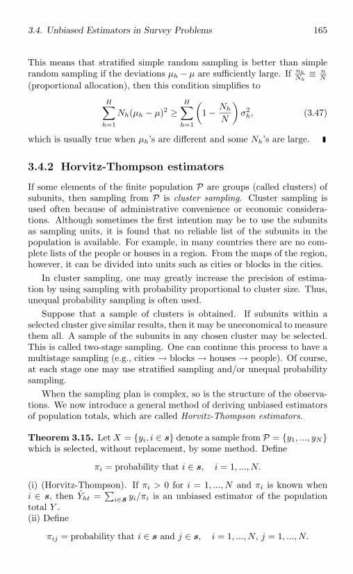
3.4. Unbiased Estimators in Survey Problems 165
This means that stratified simple random sampling is better than simplerandom sampling if the deviations µh − µ are sufficiently large. If nh
Nh≡ n
N
(proportional allocation), then this condition simplifies to
H∑h=1
Nh(µh − µ)2 ≥H∑
h=1
(1 − Nh
N
)σ2h, (3.47)
which is usually true when µh’s are different and some Nh’s are large.
3.4.2 Horvitz-Thompson estimators
If some elements of the finite population P are groups (called clusters) ofsubunits, then sampling from P is cluster sampling. Cluster sampling isused often because of administrative convenience or economic considera-tions. Although sometimes the first intention may be to use the subunitsas sampling units, it is found that no reliable list of the subunits in thepopulation is available. For example, in many countries there are no com-plete lists of the people or houses in a region. From the maps of the region,however, it can be divided into units such as cities or blocks in the cities.
In cluster sampling, one may greatly increase the precision of estima-tion by using sampling with probability proportional to cluster size. Thus,unequal probability sampling is often used.
Suppose that a sample of clusters is obtained. If subunits within aselected cluster give similar results, then it may be uneconomical to measurethem all. A sample of the subunits in any chosen cluster may be selected.This is called two-stage sampling. One can continue this process to have amultistage sampling (e.g., cities → blocks → houses → people). Of course,at each stage one may use stratified sampling and/or unequal probabilitysampling.
When the sampling plan is complex, so is the structure of the observa-tions. We now introduce a general method of deriving unbiased estimatorsof population totals, which are called Horvitz-Thompson estimators.
Theorem 3.15. Let X = yi, i ∈ s denote a sample from P = y1, ..., yNwhich is selected, without replacement, by some method. Define
πi = probability that i ∈ s, i = 1, ..., N.
(i) (Horvitz-Thompson). If πi > 0 for i = 1, ..., N and πi is known wheni ∈ s, then Yht =
∑i∈s yi/πi is an unbiased estimator of the population
total Y .(ii) Define
πij = probability that i ∈ s and j ∈ s, i = 1, ..., N, j = 1, ..., N.
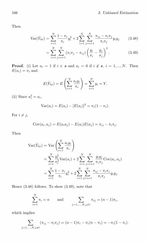
166 3. Unbiased Estimation
Then
Var(Yht) =N∑i=1
1 − πi
πiy2i + 2
N∑i=1
N∑j=i+1
πij − πiπj
πiπjyiyj (3.48)
=N∑i=1
N∑j=i+1
(πiπj − πij)(yiπi
− yjπj
)2
. (3.49)
Proof. (i) Let ai = 1 if i ∈ s and ai = 0 if i ∈ s, i = 1, ..., N . ThenE(ai) = πi and
E(Yht) = E
(N∑i=1
aiyiπi
)=
N∑i=1
yi = Y.
(ii) Since a2i = ai,
Var(ai) = E(ai) − [E(ai)]2 = πi(1 − πi).
For i = j,
Cov(ai, aj) = E(aiaj) − E(ai)E(aj) = πij − πiπj .
Then
Var(Yht) = Var
(N∑i=1
aiyiπi
)
=N∑i=1
y2i
π2i
Var(ai) + 2N∑i=1
N∑j=i+1
yiyjπiπj
Cov(ai, aj)
=N∑i=1
1 − πi
πiy2i + 2
N∑i=1
N∑j=i+1
πij − πiπj
πiπjyiyj .
Hence (3.48) follows. To show (3.49), note that
N∑i=1
πi = n and∑
j=1,...,N,j =i
πij = (n− 1)πi,
which implies∑j=1,...,N,j =i
(πij − πiπj) = (n− 1)πi − πi(n− πi) = −πi(1 − πi).
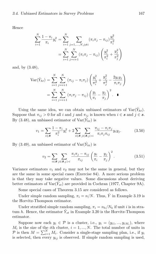
3.4. Unbiased Estimators in Survey Problems 167
Hence
N∑i=1
1 − πi
πiy2i =
N∑i=1
∑j=1,...,N,j =i
(πiπj − πij)y2i
π2i
=N∑i=1
N∑j=i+1
(πiπj − πij)
(y2i
π2i
+y2j
π2j
)
and, by (3.48),
Var(Yht) =N∑i=1
N∑j=i+1
(πij − πiπj)
(y2i
π2i
+y2j
π2j
− 2yiyjπiπj
)
=N∑i=1
N∑j=i+1
(πiπj − πij)(yiπi
− yjπj
)2
.
Using the same idea, we can obtain unbiased estimators of Var(Yht).Suppose that πij > 0 for all i and j and πij is known when i ∈ s and j ∈ s.By (3.48), an unbiased estimator of Var(Yht) is
v1 =∑i∈s
1 − πi
π2i
y2i + 2
∑i∈s
∑j∈s,j>i
πij − πiπj
πiπjπijyiyj . (3.50)
By (3.49), an unbiased estimator of Var(Yht) is
v2 =∑i∈s
∑j∈s,j>i
πiπj − πij
πij
(yiπi
− yjπj
)2
. (3.51)
Variance estimators v1 and v2 may not be the same in general, but theyare the same in some special cases (Exercise 84). A more serious problemis that they may take negative values. Some discussions about derivingbetter estimators of Var(Yst) are provided in Cochran (1977, Chapter 9A).
Some special cases of Theorem 3.15 are considered as follows.Under simple random sampling, πi = n/N . Thus, Y in Example 3.19 is
the Horvitz-Thompson estimator.Under stratified simple random sampling, πi = nh/Nh if unit i is in stra-
tum h. Hence, the estimator Yst in Example 3.20 is the Horvitz-Thompsonestimator.
Suppose now each yi ∈ P is a cluster, i.e., yi = (yi1, ..., yiMi), where
Mi is the size of the ith cluster, i = 1, ..., N . The total number of units inP is then M =
∑Ni=1 Mi. Consider a single-stage sampling plan, i.e., if yi
is selected, then every yij is observed. If simple random sampling is used,
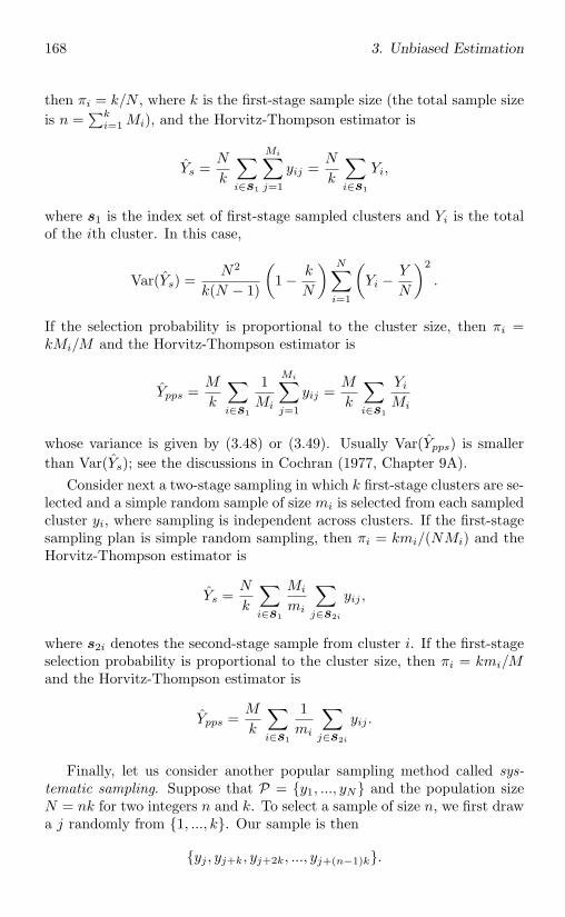
168 3. Unbiased Estimation
then πi = k/N , where k is the first-stage sample size (the total sample sizeis n =
∑ki=1 Mi), and the Horvitz-Thompson estimator is
Ys =N
k
∑i∈s1
Mi∑j=1
yij =N
k
∑i∈s1
Yi,
where s1 is the index set of first-stage sampled clusters and Yi is the totalof the ith cluster. In this case,
Var(Ys) =N2
k(N − 1)
(1 − k
N
) N∑i=1
(Yi −
Y
N
)2
.
If the selection probability is proportional to the cluster size, then πi =kMi/M and the Horvitz-Thompson estimator is
Ypps =M
k
∑i∈s1
1Mi
Mi∑j=1
yij =M
k
∑i∈s1
Yi
Mi
whose variance is given by (3.48) or (3.49). Usually Var(Ypps) is smallerthan Var(Ys); see the discussions in Cochran (1977, Chapter 9A).
Consider next a two-stage sampling in which k first-stage clusters are se-lected and a simple random sample of size mi is selected from each sampledcluster yi, where sampling is independent across clusters. If the first-stagesampling plan is simple random sampling, then πi = kmi/(NMi) and theHorvitz-Thompson estimator is
Ys =N
k
∑i∈s1
Mi
mi
∑j∈s2i
yij ,
where s2i denotes the second-stage sample from cluster i. If the first-stageselection probability is proportional to the cluster size, then πi = kmi/Mand the Horvitz-Thompson estimator is
Ypps =M
k
∑i∈s1
1mi
∑j∈s2i
yij .
Finally, let us consider another popular sampling method called sys-tematic sampling. Suppose that P = y1, ..., yN and the population sizeN = nk for two integers n and k. To select a sample of size n, we first drawa j randomly from 1, ..., k. Our sample is then
yj , yj+k, yj+2k, ..., yj+(n−1)k.
3.4. Unbiased Estimators in Survey Problems 169
Systematic sampling is used mainly because it is easier to draw a systematicsample and often easier to execute without mistakes. It is also likely thatsystematic sampling provides more efficient point estimators than simplerandom sampling or even stratified sampling, since the sample units arespread more evenly over the population. Under systematic sampling, πi =k−1 for every i and the Horvitz-Thompson estimator of the population totalis
Ysy = k
n∑t=1
yj+(t−1)k.
The unbiasedness of this estimator is a direct consequence of Theorem 3.15,but it can be easily shown as follows. Since j takes value i ∈ 1, ..., k withprobability k−1,
E(Ysy) = k
(1k
k∑i=1
n∑t=1
yi+(t−1)k
)=
N∑i=1
yi = Y.
The variance of Ysy is simply
Var(Ysy) =N2
k
k∑i=1
(µi − µ)2,
where µi = n−1 ∑nt=1 yi+(t−1)k and µ = k−1 ∑k
i=1 µi = Y/N . Let σ2 begiven by (3.44) and
σ2sy =
1k(n− 1)
k∑i=1
n∑t=1
(yi+(t−1)k − µi)2.
Then
(N − 1)σ2 = n
k∑i=1
(µi − µ)2 +k∑
i=1
n∑t=1
(yi+(t−1)k − µi)2.
Thus,(N − 1)σ2 = N−1Var(Ysy) + k(n− 1)σ2
sy
andVar(Ysy) = N(N − 1)σ2 −N(N − k)σ2
sy.
Since the variance of the Horvitz-Thompson estimator of the populationtotal under simple random sampling is, by (3.44),
N2
n
(1 − n
N
)σ2 = N(k − 1)σ2,
the Horvitz-Thompson estimator under systematic sampling has a smallervariance if and only if σ2
sy > σ2.
170 3. Unbiased Estimation
3.5 Asymptotically Unbiased Estimators
As we discussed in §2.5, we often need to consider biased but asymptoti-cally unbiased estimators. A large and useful class of such estimators aresmooth functions of some exactly unbiased estimators such as UMVUE’s,U-statistics, and LSE’s. Some other methods of constructing asymptoti-cally unbiased estimators are also introduced in this section.
3.5.1 Functions of unbiased estimators
If the parameter to be estimated is ϑ = g(θ) with a vector-valued parameterθ and Un is a vector of unbiased estimators of components of θ (i.e., EUn =θ), then Tn = g(Un) is asymptotically unbiased for ϑ. Assume that g issecond-order differentiable and ‖Un − θ‖ = op(1). Then
bTn(P ) = tr(∇2g(θ)Var(Un))/2
andamseTn(P ) = ∇g(θ)Var(Un)[∇g(θ)]τ
(Theorem 2.6). Hence, Tn has a good performance in terms of amse if Un
is optimal in terms of mse (such as the UMVUE).The following are some examples.
Example 3.21 (Ratio estimators). Let (X1, Y1), ..., (Xn, Yn) be i.i.d. ran-dom 2-vectors. Consider the estimation of the ratio of two populationmeans: ϑ = µy/µx (µx = 0). Note that (Y , X), the vector of samplemeans, is unbiased for (µy, µx). The sample means are UMVUE’s undersome statistical models (§3.1 and §3.2) and are BLUE’s in general (Exam-ple 2.22). The ratio estimator is Tn = Y /X. Assume that σ2
x = Var(X1),σ2y = Var(Y1), and σxy = Cov(X1, Y1) exist. A direct calculation shows
that
bTn(P ) =ϑσ2
x − σxy
µ2xn
, (3.52)
and√n(Tn − ϑ) →d N
(0,
σ2y − 2ϑσxy + ϑ2σ2
x
µ2x
), (3.53)
which implies
amseTn(P ) =
σ2y − 2ϑσxy + ϑ2σ2
x
µ2xn
. (3.54)
Results (3.52) and (3.54) still hold when (X1, Y1), ..., (Xn, Yn) is a samplefrom a finite bivariate population of size N (exercise). In some problems we
3.5. Asymptotically Unbiased Estimators 171
are not interested in the ratio, but the use of a ratio estimator to improvean estimator of a marginal mean. For example, suppose that µx is knownand we are interested in estimating µy. Consider the following estimator
µy = (Y /X)µx.
Note that µy is not unbiased; its n−1 order asymptotic bias is
bµy (P ) =ϑσ2
x − σxy
µxn;
and
amseµy(P ) =
σ2y − 2ϑσxy + ϑ2σ2
x
n.
Comparing µy with the unbiased estimator Y , we find that µy is asymp-totically more efficient if and only if
2ϑσxy > ϑ2σ2x,
which means that µy is a better estimator if and only if the correlationbetween X1 and Y1 is large enough to pay off the extra variability causedby using µx/X.
Another example related to a bivariate sample is the sample correlationcoefficient defined in Exercise 19 in §2.6.
Example 3.22. Consider a polynomial regression of order p:
Xi = βZτi + εi, i = 1, ..., n,
where β = (β0, β1, ..., βp−1), Zi = (1, ti, ..., tp−1i ), and εi’s are i.i.d. with
mean 0 and variance σ2 > 0. Suppose that the parameter to be estimatedis tβ ∈ R such that
p−1∑j=0
βjtjβ = max
t∈R
p−1∑j=0
βjtj .
Note that tβ = g(β) for some function g. Let β be the LSE of β. Then theestimator tβ = g(β) is asymptotically unbiased and its amse can be derivedunder some conditions (exercise).
Example 3.23. In the study of the reliability of a system component, weassume that
Xij = z(tj)θτi + εij , i = 1, ..., k, j = 1, ...,m.
172 3. Unbiased Estimation
Here Xij is the measurement of the ith sample component at time tj ; z(t)is a q-vector whose components are known functions of the time t; θi’sare unobservable random q-vectors that are i.i.d. from Nq(θ,Σ), where θand Σ are unknown; εij ’s are i.i.d. measurement errors with mean zeroand variance σ2; and θi’s and εij ’s are independent. As a function of t,z(t)θτ is the degradation curve for a particular component and z(t)θτ isthe mean degradation curve. Suppose that a component will fail to work ifz(t)θτ < η, a given critical value. Assume that z(t)′θ is always a decreasingfunction of t. Then the reliability function of a component is
R(t) = P (z(t)θτ > η) = Φ(z(t)θτ − η
s(t)
),
where s(t) =√z(t)Σ[z(t)]τ and Φ is the standard normal distribution
function. For a fixed t, estimators of R(t) can be obtained by estimatingθ and Σ, since Φ is a known function. It can be shown (exercise) that theBLUE of θ is the LSE
θ = XZ(ZτZ)−1,
where Z = ([z(t1)]τ , ...., [z(tk)]τ )τ , Xi = (Xi1, ..., Xim), and X is the samplemean of Xi’s. The estimation of Σ is more difficult. An asymptoticallyunbiased (as k → ∞) estimator of Σ is
Σ =1k
k∑i=1
(ZτZ)−1Zτ (Xi − X)τ (Xi − X)Z(ZτZ)−1 − σ2(ZτZ)−1,
where
σ2 =1
k(m− q)
k∑i=1
[XiXτi −XiZ(ZτZ)−1ZτXτ
i ].
Hence an estimator of R(t) is
R(t) = Φ
(z(t)θτ − η
s(t)
),
where
s(t) =z(t)Σ[z(t)]τ
1/2.
If we define Yi1 = XiZ(ZτZ)−1[z(t)]τ , Yi2 = XiZ(ZτZ)−1[z(t)]τ2, Yi3 =[XiX
τi − XiZ(ZτZ)−1ZτXτ
i ]/(m − q) and Yi = (Yi1, Yi2, Yi3)′, then it isapparent that R(t) can be written as g(Y ) for a function
g(y1, y2, y3) = Φ
(y1 − η√
y2 − y21 − y3z(t)(ZτZ)−1[z(t)]τ
).
Suppose that εij has a finite fourth moment, which implies the existence ofVar(Yi). The amse of R(t) can be derived (exercise).
3.5. Asymptotically Unbiased Estimators 173
3.5.2 The method of moments
The method of moments is the oldest method of deriving point estima-tors. It almost always produces some asymptotically unbiased estimators,although they may not be the best estimators.
Consider a parametric problem where X1, ..., Xn are i.i.d. random vari-ables from Pθ, θ ∈ Θ ⊂ Rk, and E|X1|k < ∞. Let µj = EXj
1 be the jthmoment of P and let
µj =1n
n∑i=1
Xji
be the jth sample moment, which is an unbiased estimator of µj , j = 1, ..., k.Typically,
µj = hj(θ), j = 1, ..., k, (3.55)
for some functions hj on Rk. By substituting µj ’s on the left-hand side of(3.55) by the sample moments µj , we obtain a moment estimator θ, i.e., θsatisfies
µj = hj(θ), j = 1, ..., k,
which is a sample analogue of (3.55). This method of deriving estimators iscalled the method of moments. Note that an important statistical principle,the substitution principle, is applied in this method.
Let µ = (µ1, ..., µk) and h = (h1, ..., hk). Then µ = h(θ). If h−1 exists,then the unique moment estimator of θ is θ = h−1(µ). When h−1 doesnot exist (i.e., h is not one-to-one), any solution of µ = h(θ), denoted byθ = g(µ), is a moment estimator of θ.
By the SLLN, µj →a.s. µj . Assume that h is one-to-one and let g = h−1.Typically, the function g in θ = g(µ) is continuous and, therefore, θ isstrongly consistent for θ. If g is differentiable and E|X1|2k < ∞, then θ isasymptotically normal, by the CLT and Theorem 2.11, and
amseθ(θ) = n−1∇g(µ)Vµ[∇g(µ)]τ , (3.56)
where µ = (µ1, ..., µk) and Vµ is a k × k matrix whose (i, j)th element isµi+j − µiµj .
Example 3.24. Let X1, ..., Xn be i.i.d. from a population Pθ indexed bythe parameter θ = (µ, σ2), where µ = EX1 ∈ R and σ2 = Var(X1) ∈(0,∞). This includes cases like the family of normal distributions, dou-ble exponential distributions, or logistic distributions (Table 1.2, page 20).Since EX1 = µ and EX2
1 = Var(X1) + (EX1)2 = σ2 + µ2, setting µ1 = µand µ2 = σ2 + µ2 we obtain the moment estimators
θ =
(X,
1n
n∑i=1
(Xi − X)2)
=(X,
n− 1n
S2).
174 3. Unbiased Estimation
Note that X is unbiased, but n−1n S2 is not. If Xi is normal, then θ is suffi-
cient and is nearly the same as an optimal estimator such as the UMVUE.On the other hand, if Xi is from a double exponential or logistic distribu-tion, then θ is not sufficient and can often be improved.
Consider now the estimation of σ2 when we know that µ = 0. Obviouslywe cannot use the equation µ1 = µ to solve the problem. Using µ2 = µ2 =σ2, we obtain the moment estimator σ2 = µ2 = n−1 ∑n
i=1 X2i . This is
still a good estimator when Xi is normal, but is not a function of sufficientstatistic when Xi is from a double exponential distribution. For the doubleexponential case one can argue that we should first make a transformationYi = |Xi| and then obtain the moment estimator based on the transformeddata. The moment estimator of σ2 based on the transformed data is Y =n−1 ∑n
i=1 |Xi|, which is sufficient for σ2. Note that this estimator can alsobe obtained based on absolute moment equations.
Example 3.25. Let X1, ..., Xn be i.i.d. from the uniform distribution on(θ1, θ2), −∞ < θ1 < θ2 < ∞. Note that
EX1 = (θ1 + θ2)/2
andEX2
1 = (θ21 + θ2
2 + θ1θ2)/3.
Setting µ1 = EX1 and µ2 = EX21 and substituting θ1 in the second equa-
tion by 2µ1 − θ2 (the first equation), we obtain that
(2µ1 − θ2)2 + θ22 + (2µ1 − θ2)θ2 = 3µ2,
which is the same as
(θ2 − µ1)2 = 3(µ2 − µ21).
Since θ2 ≥ µ1, we obtain that
θ2 = µ1 +√
3(µ2 − µ21) = X +
√3(n−1)
n S2
andθ1 = µ1 −
√3(µ2 − µ2
1) = X −√
3(n−1)n S2.
These estimators are not functions of the sufficient and complete statistic(X(1), X(n)).
Example 3.26. Let X1, ..., Xn be i.i.d. from the binomial distributionBi(p, k) with unknown parameters k ∈ 1, 2, ... and p ∈ (0, 1). Since
EX1 = kp
3.5. Asymptotically Unbiased Estimators 175
andEX2
1 = kp(1 − p) + k2p2,
we obtain the moment estimators
p = (µ1 + µ21 − µ2)/µ1 = 1 − n−1
n S2/X
andk = µ2
1/(µ1 + µ21 − µ2) = X/(1 − n−1
n S2/X).
The estimator p is in the range of (0, 1). But k may not be an integer. Itcan be improved by an estimator which is k rounded to the nearest positiveinteger.
Example 3.27. Suppose that X1, ..., Xn are i.i.d. from the Pareto distri-bution Pa(a, θ) with unknown a > 0 and θ > 2 (Table 1.2, page 20). Notethat
EX1 = θa/(θ − 1)
andEX2
1 = θa2/(θ − 2).
From the moment equation,
(θ−1)2
θ(θ−2) = µ2/µ21.
Note that (θ−1)2
θ(θ−2) − 1 = 1θ(θ−2) . Hence
θ(θ − 2) = µ21/(µ2 − µ2
1).
Since θ > 2, there is a unique solution
θ = 1 +√µ2/(µ2 − µ2
1) = 1 +√
1 + nn−1X
2/S2
and
a =µ1(θ − 1)
θ
= X√
1 + nn−1X
2/S2/(
1 +√
1 + nn−1X
2/S2).
The method of moments can also be applied to nonparametric problems.Consider, for example, the estimation of the central moments
cj = E(X1 − µ)j , j = 2, ..., k.
176 3. Unbiased Estimation
Since
cj =j∑
t=0
(j
t
)(−µ)tµj−t,
the moment estimator of cj is
cj =j∑
t=0
(j
t
)(−X)tµj−t,
where µ0 = 1. It can be shown (exercise) that
cj =1n
n∑i=1
(Xi − X)j , j = 2, ..., k, (3.57)
which are sample central moments. From the SLLN, cj ’s are strongly con-sistent. If E|X1|2k < ∞, then
√n (c2 − c2, ..., ck − ck) →d Nk−1(0, D) (3.58)
(exercise), where the (i, j)th element of the (k − 1) × (k − 1) matrix D is
ci+j+2 − ci+1cj+1 − (i + 1)cicj+2 − (j + 1)ci+2cj + (i + 1)(j + 1)cicjc2.
3.5.3 V-statistics
Let X1, ..., Xn be i.i.d. from P . For every U-statistic defined in (3.11) asan estimator of ϑ = E[h(X1, ..., Xm)], there is a closely related V-statisticdefined by
Vn =1nm
n∑i1=1
· · ·n∑
im=1
h(Xi1 , ..., Xim). (3.59)
As an estimator of ϑ, Vn is biased; but the bias is small asymptotically asthe following results show. For a fixed sample size n, Vn may be better thanUn in terms of their mse’s. Consider, for example, the kernel h(x1, x2) =(x1 − x2)2/2 in §3.2.1, which leads to ϑ = σ2 = Var(X1) and Un = S2, thesample variance. The corresponding V-statistic is
1n2
n∑i=1
n∑j=1
(Xi −Xj)2
2=
1n2
∑1≤i<j≤n
(Xi −Xj)2 =n− 1n
S2,
which is the moment estimator of σ2 discussed in Example 3.24. In Ex-ercise 52 in §2.6, n−1
n S2 is shown to have a smaller mse than S2 in somecases. Of course, there are situations where U-statistics are better thantheir corresponding V-statistics.
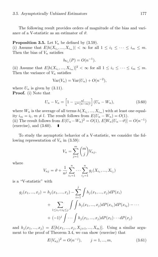
3.5. Asymptotically Unbiased Estimators 177
The following result provides orders of magnitude of the bias and vari-ance of a V-statistic as an estimator of ϑ.
Proposition 3.5. Let Vn be defined by (3.59).(i) Assume that E|h(Xi1 , ..., Xim)| < ∞ for all 1 ≤ i1 ≤ · · · ≤ im ≤ m.Then the bias of Vn satisfies
bVn(P ) = O(n−1).
(ii) Assume that E[h(Xi1 , ..., Xim)]2 < ∞ for all 1 ≤ i1 ≤ · · · ≤ im ≤ m.Then the variance of Vn satisfies
Var(Vn) = Var(Un) + O(n−2),
where Un is given by (3.11).Proof. (i) Note that
Un − Vn =[1 − n!
nm(n−m)!
](Un −Wn), (3.60)
where Wn is the average of all terms h(Xi1 , ..., Xim) with at least one equal-ity im = il, m = l. The result follows from E(Un −Wn) = O(1).(ii) The result follows from E(Un−Wn)2 = O(1), E[Wn(Un−ϑ)] = O(n−1)(exercise), and (3.60).
To study the asymptotic behavior of a V-statistic, we consider the fol-lowing representation of Vn in (3.59):
Vn =m∑j=1
(m
j
)Vnj ,
where
Vnj = ϑ +1nj
n∑i1=1
· · ·n∑
ij=1
gj(Xi1 , ..., Xij )
is a “V-statistic” with
gj(x1, ..., xj) = hj(x1, ..., xj) −j∑
i=1
∫hj(x1, ..., xj)dP (xi)
+∑
1≤i1<i2≤j
∫ ∫hj(x1, ..., xj)dP (xi1)dP (xi2) − · · ·
+ (−1)j∫
· · ·∫
hj(x1, ..., xj)dP (x1) · · · dP (xj)
and hj(x1, ..., xj) = E[h(x1, ..., xj , Xj+1, ..., Xm)]. Using a similar argu-ment to the proof of Theorem 3.4, we can show (exercise) that
E(Vnj)2 = O(n−j), j = 1, ...,m, (3.61)
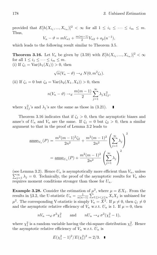
178 3. Unbiased Estimation
provided that E[h(Xi1 , ..., Xim)]2 < ∞ for all 1 ≤ i1 ≤ · · · ≤ im ≤ m.Thus,
Vn − ϑ = mVn1 + m(m−1)2 Vn2 + op(n−1),
which leads to the following result similar to Theorem 3.5.
Theorem 3.16. Let Vn be given by (3.59) with E[h(Xi1 , ..., Xim)]2 < ∞for all 1 ≤ i1 ≤ · · · ≤ im ≤ m.(i) If ζ1 = Var(h1(X1)) > 0, then
√n(Vn − ϑ) →d N(0,m2ζ1).
(ii) If ζ1 = 0 but ζ2 = Var(h2(X1, X2)) > 0, then
n(Vn − ϑ) →dm(m− 1)
2
∞∑j=1
λjχ21j ,
where χ21j ’s and λj ’s are the same as those in (3.21).
Theorem 3.16 indicates that if ζ1 > 0, then the asymptotic biases andamse’s of Un and Vn are the same. If ζ1 = 0 but ζ2 > 0, then a similarargument to that in the proof of Lemma 3.2 leads to
amseVn(P ) =
m2(m− 1)2ζ22n2 +
m2(m− 1)2
2n2
⎛⎝ ∞∑j=1
λj
⎞⎠2
= amseUn(P ) +
m2(m− 1)2
2n2
⎛⎝ ∞∑j=1
λj
⎞⎠2
(see Lemma 3.2). Hence Un is asymptotically more efficient than Vn, unless∑∞j=1 λj = 0. Technically, the proof of the asymptotic results for Vn also
requires moment conditions stronger than those for Un.
Example 3.28. Consider the estimation of µ2, where µ = EX1. From theresults in §3.2, the U-statistic Un = 1
n(n−1)
∑1≤i<j≤n XiXj is unbiased for
µ2. The corresponding V-statistic is simply Vn = X2. If µ = 0, then ζ1 = 0and the asymptotic relative efficiency of Vn w.r.t. Un is 1. If µ = 0, then
nVn →d σ2χ21 and nUn →d σ2(χ2
1 − 1),
where χ21 is a random variable having the chi-square distribution χ2
1. Hencethe asymptotic relative efficiency of Vn w.r.t. Un is
E(χ21 − 1)2/E(χ2
1)2 = 2/3.
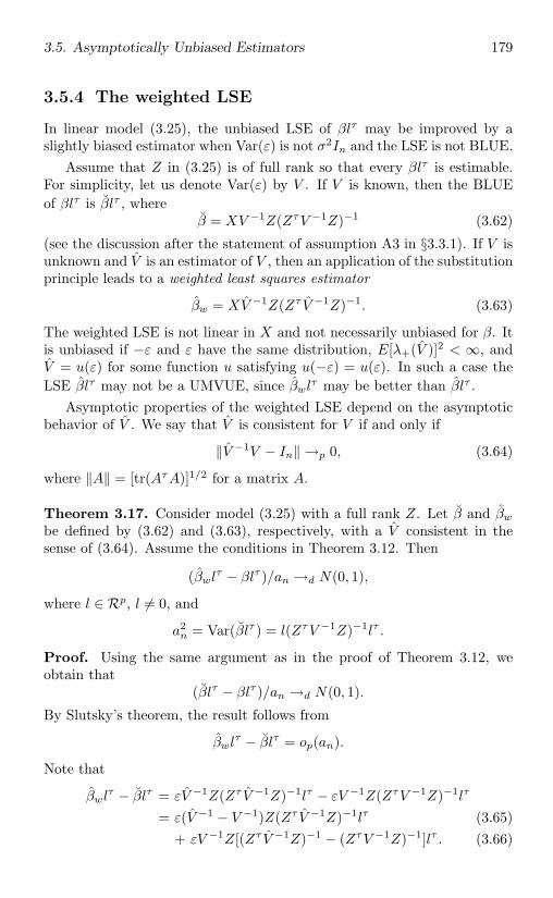
3.5. Asymptotically Unbiased Estimators 179
3.5.4 The weighted LSE
In linear model (3.25), the unbiased LSE of βlτ may be improved by aslightly biased estimator when Var(ε) is not σ2In and the LSE is not BLUE.
Assume that Z in (3.25) is of full rank so that every βlτ is estimable.For simplicity, let us denote Var(ε) by V . If V is known, then the BLUEof βlτ is βlτ , where
β = XV −1Z(ZτV −1Z)−1 (3.62)
(see the discussion after the statement of assumption A3 in §3.3.1). If V isunknown and V is an estimator of V , then an application of the substitutionprinciple leads to a weighted least squares estimator
βw = XV −1Z(Zτ V −1Z)−1. (3.63)
The weighted LSE is not linear in X and not necessarily unbiased for β. Itis unbiased if −ε and ε have the same distribution, E[λ+(V )]2 < ∞, andV = u(ε) for some function u satisfying u(−ε) = u(ε). In such a case theLSE βlτ may not be a UMVUE, since βwl
τ may be better than βlτ .Asymptotic properties of the weighted LSE depend on the asymptotic
behavior of V . We say that V is consistent for V if and only if
‖V −1V − In‖ →p 0, (3.64)
where ‖A‖ = [tr(AτA)]1/2 for a matrix A.
Theorem 3.17. Consider model (3.25) with a full rank Z. Let β and βw
be defined by (3.62) and (3.63), respectively, with a V consistent in thesense of (3.64). Assume the conditions in Theorem 3.12. Then
(βwlτ − βlτ )/an →d N(0, 1),
where l ∈ Rp, l = 0, and
a2n = Var(βlτ ) = l(ZτV −1Z)−1lτ .
Proof. Using the same argument as in the proof of Theorem 3.12, weobtain that
(βlτ − βlτ )/an →d N(0, 1).
By Slutsky’s theorem, the result follows from
βwlτ − βlτ = op(an).
Note that
βwlτ − βlτ = εV −1Z(Zτ V −1Z)−1lτ − εV −1Z(ZτV −1Z)−1lτ
= ε(V −1 − V −1)Z(Zτ V −1Z)−1lτ (3.65)+ εV −1Z[(Zτ V −1Z)−1 − (ZτV −1Z)−1]lτ . (3.66)
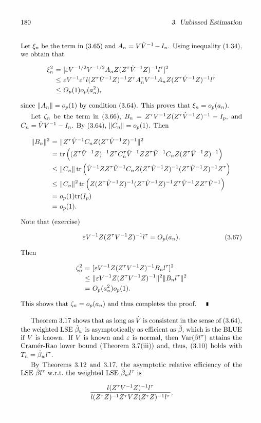
180 3. Unbiased Estimation
Let ξn be the term in (3.65) and An = V V −1− In. Using inequality (1.34),we obtain that
ξ2n = [εV −1/2V −1/2AnZ(Zτ V −1Z)−1lτ ]2
≤ εV −1ετ l(Zτ V −1Z)−1ZτAτnV
−1AnZ(Zτ V −1Z)−1lτ
≤ Op(1)op(a2n),
since ‖An‖ = op(1) by condition (3.64). This proves that ξn = op(an).
Let ζn be the term in (3.66), Bn = ZτV −1Z(Zτ V −1Z)−1 − Ip, andCn = V V −1 − In. By (3.64), ‖Cn‖ = op(1). Then
‖Bn‖2 = ‖Zτ V −1CnZ(Zτ V −1Z)−1‖2
= tr((Zτ V −1Z)−1ZτCτ
nV−1ZZτ V −1CnZ(Zτ V −1Z)−1
)≤ ‖Cn‖ tr
(V −1ZZτ V −1CnZ(Zτ V −1Z)−1(Zτ V −1Z)−1Zτ
)≤ ‖Cn‖2 tr
(Z(Zτ V −1Z)−1(Zτ V −1Z)−1Zτ V −1ZZτ V −1
)= op(1)tr(Ip)= op(1).
Note that (exercise)
εV −1Z(ZτV −1Z)−1lτ = Op(an). (3.67)
Then
ζ2n = [εV −1Z(ZτV −1Z)−1Bnl
τ ]2
≤ ‖εV −1Z(ZτV −1Z)−1‖2‖Bnlτ‖2
= Op(a2n)op(1).
This shows that ζn = op(an) and thus completes the proof.
Theorem 3.17 shows that as long as V is consistent in the sense of (3.64),the weighted LSE βw is asymptotically as efficient as β, which is the BLUEif V is known. If V is known and ε is normal, then Var(βlτ ) attains theCramer-Rao lower bound (Theorem 3.7(iii)) and, thus, (3.10) holds withTn = βwl
τ .By Theorems 3.12 and 3.17, the asymptotic relative efficiency of the
LSE βlτ w.r.t. the weighted LSE βwlτ is
l(ZτV −1Z)−1lτ
l(ZτZ)−1ZτV Z(ZτZ)−1lτ,
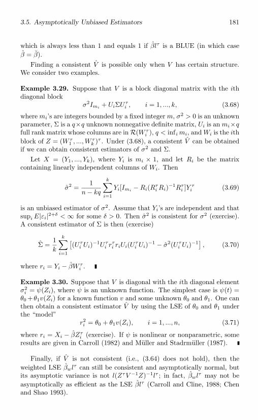
3.5. Asymptotically Unbiased Estimators 181
which is always less than 1 and equals 1 if βlτ is a BLUE (in which caseβ = β).
Finding a consistent V is possible only when V has certain structure.We consider two examples.
Example 3.29. Suppose that V is a block diagonal matrix with the ithdiagonal block
σ2Imi + UiΣUτi , i = 1, ..., k, (3.68)
where mi’s are integers bounded by a fixed integer m, σ2 > 0 is an unknownparameter, Σ is a q×q unknown nonnegative definite matrix, Ui is an mi×qfull rank matrix whose columns are in R(W τ
i ), q < infi mi, and Wi is the ithblock of Z = (W τ
1 , ...,Wτk )τ . Under (3.68), a consistent V can be obtained
if we can obtain consistent estimators of σ2 and Σ.Let X = (Y1, ..., Yk), where Yi is mi × 1, and let Ri be the matrix
containing linearly independent columns of Wi. Then
σ2 =1
n− kq
k∑i=1
Yi[Imi −Ri(Rτi Ri)−1Rτ
i ]Y τi (3.69)
is an unbiased estimator of σ2. Assume that Yi’s are independent and thatsupi E|εi|2+δ < ∞ for some δ > 0. Then σ2 is consistent for σ2 (exercise).A consistent estimator of Σ is then (exercise)
Σ =1k
k∑i=1
[(Uτ
i Ui)−1Uτi r
τi riUi(Uτ
i Ui)−1 − σ2(Uτi Ui)−1] , (3.70)
where ri = Yi − βW τi .
Example 3.30. Suppose that V is diagonal with the ith diagonal elementσ2i = ψ(Zi), where ψ is an unknown function. The simplest case is ψ(t) =
θ0 + θ1v(Zi) for a known function v and some unknown θ0 and θ1. One canthen obtain a consistent estimator V by using the LSE of θ0 and θ1 underthe “model”
r2i = θ0 + θ1v(Zi), i = 1, ..., n, (3.71)
where ri = Xi − βZτi (exercise). If ψ is nonlinear or nonparametric, some
results are given in Carroll (1982) and Muller and Stadrmuller (1987).
Finally, if V is not consistent (i.e., (3.64) does not hold), then theweighted LSE βwl
τ can still be consistent and asymptotically normal, butits asymptotic variance is not l(ZτV −1Z)−1lτ ; in fact, βwl
τ may not beasymptotically as efficient as the LSE βlτ (Carroll and Cline, 1988; Chenand Shao 1993).
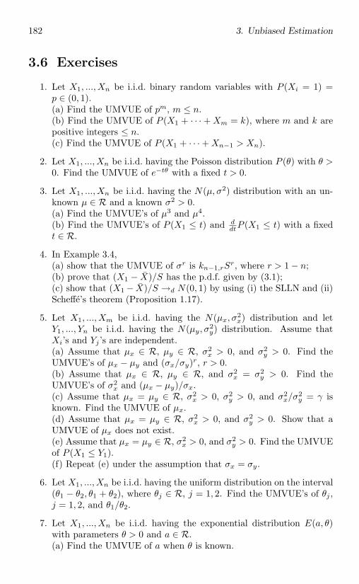
182 3. Unbiased Estimation
3.6 Exercises
1. Let X1, ..., Xn be i.i.d. binary random variables with P (Xi = 1) =p ∈ (0, 1).(a) Find the UMVUE of pm, m ≤ n.(b) Find the UMVUE of P (X1 + · · · + Xm = k), where m and k arepositive integers ≤ n.(c) Find the UMVUE of P (X1 + · · · + Xn−1 > Xn).
2. Let X1, ..., Xn be i.i.d. having the Poisson distribution P (θ) with θ >0. Find the UMVUE of e−tθ with a fixed t > 0.
3. Let X1, ..., Xn be i.i.d. having the N(µ, σ2) distribution with an un-known µ ∈ R and a known σ2 > 0.(a) Find the UMVUE’s of µ3 and µ4.(b) Find the UMVUE’s of P (X1 ≤ t) and d
dtP (X1 ≤ t) with a fixedt ∈ R.
4. In Example 3.4,(a) show that the UMVUE of σr is kn−1,rS
r, where r > 1 − n;(b) prove that (X1 − X)/S has the p.d.f. given by (3.1);(c) show that (X1 − X)/S →d N(0, 1) by using (i) the SLLN and (ii)Scheffe’s theorem (Proposition 1.17).
5. Let X1, ..., Xm be i.i.d. having the N(µx, σ2x) distribution and let
Y1, ..., Yn be i.i.d. having the N(µy, σ2y) distribution. Assume that
Xi’s and Yj ’s are independent.(a) Assume that µx ∈ R, µy ∈ R, σ2
x > 0, and σ2y > 0. Find the
UMVUE’s of µx − µy and (σx/σy)r, r > 0.(b) Assume that µx ∈ R, µy ∈ R, and σ2
x = σ2y > 0. Find the
UMVUE’s of σ2x and (µx − µy)/σx.
(c) Assume that µx = µy ∈ R, σ2x > 0, σ2
y > 0, and σ2x/σ
2y = γ is
known. Find the UMVUE of µx.(d) Assume that µx = µy ∈ R, σ2
x > 0, and σ2y > 0. Show that a
UMVUE of µx does not exist.(e) Assume that µx = µy ∈ R, σ2
x > 0, and σ2y > 0. Find the UMVUE
of P (X1 ≤ Y1).(f) Repeat (e) under the assumption that σx = σy.
6. Let X1, ..., Xn be i.i.d. having the uniform distribution on the interval(θ1 − θ2, θ1 + θ2), where θj ∈ R, j = 1, 2. Find the UMVUE’s of θj ,j = 1, 2, and θ1/θ2.
7. Let X1, ..., Xn be i.i.d. having the exponential distribution E(a, θ)with parameters θ > 0 and a ∈ R.(a) Find the UMVUE of a when θ is known.
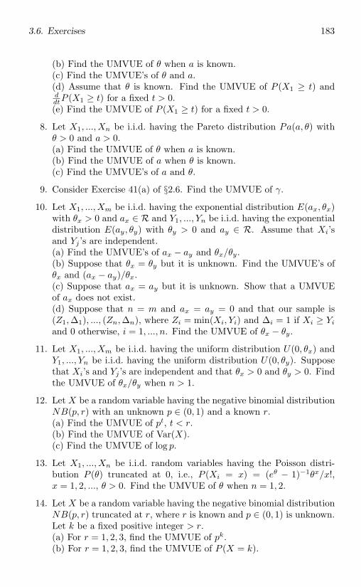
3.6. Exercises 183
(b) Find the UMVUE of θ when a is known.(c) Find the UMVUE’s of θ and a.(d) Assume that θ is known. Find the UMVUE of P (X1 ≥ t) andddtP (X1 ≥ t) for a fixed t > 0.(e) Find the UMVUE of P (X1 ≥ t) for a fixed t > 0.
8. Let X1, ..., Xn be i.i.d. having the Pareto distribution Pa(a, θ) withθ > 0 and a > 0.(a) Find the UMVUE of θ when a is known.(b) Find the UMVUE of a when θ is known.(c) Find the UMVUE’s of a and θ.
9. Consider Exercise 41(a) of §2.6. Find the UMVUE of γ.
10. Let X1, ..., Xm be i.i.d. having the exponential distribution E(ax, θx)with θx > 0 and ax ∈ R and Y1, ..., Yn be i.i.d. having the exponentialdistribution E(ay, θy) with θy > 0 and ay ∈ R. Assume that Xi’sand Yj ’s are independent.(a) Find the UMVUE’s of ax − ay and θx/θy.(b) Suppose that θx = θy but it is unknown. Find the UMVUE’s ofθx and (ax − ay)/θx.(c) Suppose that ax = ay but it is unknown. Show that a UMVUEof ax does not exist.(d) Suppose that n = m and ax = ay = 0 and that our sample is(Z1,∆1), ..., (Zn,∆n), where Zi = min(Xi, Yi) and ∆i = 1 if Xi ≥ Yi
and 0 otherwise, i = 1, ..., n. Find the UMVUE of θx − θy.
11. Let X1, ..., Xm be i.i.d. having the uniform distribution U(0, θx) andY1, ..., Yn be i.i.d. having the uniform distribution U(0, θy). Supposethat Xi’s and Yj ’s are independent and that θx > 0 and θy > 0. Findthe UMVUE of θx/θy when n > 1.
12. Let X be a random variable having the negative binomial distributionNB(p, r) with an unknown p ∈ (0, 1) and a known r.(a) Find the UMVUE of pt, t < r.(b) Find the UMVUE of Var(X).(c) Find the UMVUE of log p.
13. Let X1, ..., Xn be i.i.d. random variables having the Poisson distri-bution P (θ) truncated at 0, i.e., P (Xi = x) = (eθ − 1)−1θx/x!,x = 1, 2, ..., θ > 0. Find the UMVUE of θ when n = 1, 2.
14. Let X be a random variable having the negative binomial distributionNB(p, r) truncated at r, where r is known and p ∈ (0, 1) is unknown.Let k be a fixed positive integer > r.(a) For r = 1, 2, 3, find the UMVUE of pk.(b) For r = 1, 2, 3, find the UMVUE of P (X = k).
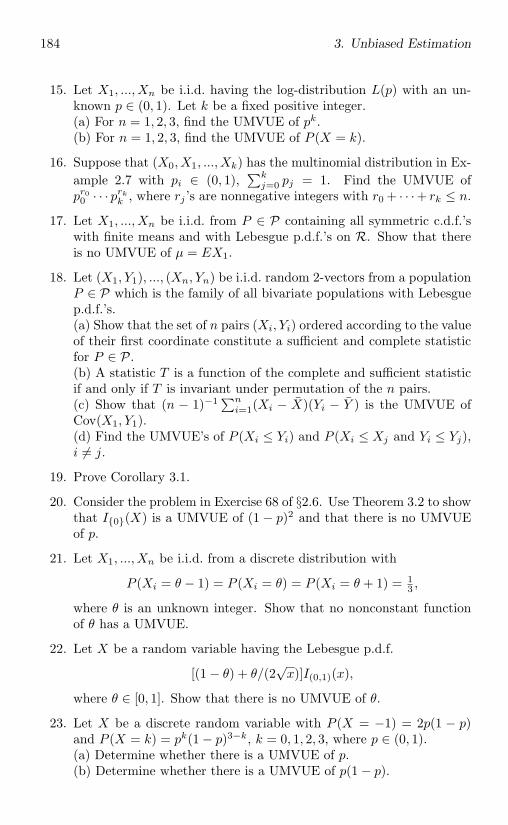
184 3. Unbiased Estimation
15. Let X1, ..., Xn be i.i.d. having the log-distribution L(p) with an un-known p ∈ (0, 1). Let k be a fixed positive integer.(a) For n = 1, 2, 3, find the UMVUE of pk.(b) For n = 1, 2, 3, find the UMVUE of P (X = k).
16. Suppose that (X0, X1, ..., Xk) has the multinomial distribution in Ex-ample 2.7 with pi ∈ (0, 1),
∑kj=0 pj = 1. Find the UMVUE of
pr00 · · · prkk , where rj ’s are nonnegative integers with r0 + · · ·+ rk ≤ n.
17. Let X1, ..., Xn be i.i.d. from P ∈ P containing all symmetric c.d.f.’swith finite means and with Lebesgue p.d.f.’s on R. Show that thereis no UMVUE of µ = EX1.
18. Let (X1, Y1), ..., (Xn, Yn) be i.i.d. random 2-vectors from a populationP ∈ P which is the family of all bivariate populations with Lebesguep.d.f.’s.(a) Show that the set of n pairs (Xi, Yi) ordered according to the valueof their first coordinate constitute a sufficient and complete statisticfor P ∈ P.(b) A statistic T is a function of the complete and sufficient statisticif and only if T is invariant under permutation of the n pairs.(c) Show that (n − 1)−1 ∑n
i=1(Xi − X)(Yi − Y ) is the UMVUE ofCov(X1, Y1).(d) Find the UMVUE’s of P (Xi ≤ Yi) and P (Xi ≤ Xj and Yi ≤ Yj),i = j.
19. Prove Corollary 3.1.
20. Consider the problem in Exercise 68 of §2.6. Use Theorem 3.2 to showthat I0(X) is a UMVUE of (1 − p)2 and that there is no UMVUEof p.
21. Let X1, ..., Xn be i.i.d. from a discrete distribution with
P (Xi = θ − 1) = P (Xi = θ) = P (Xi = θ + 1) = 13 ,
where θ is an unknown integer. Show that no nonconstant functionof θ has a UMVUE.
22. Let X be a random variable having the Lebesgue p.d.f.
[(1 − θ) + θ/(2√x)]I(0,1)(x),
where θ ∈ [0, 1]. Show that there is no UMVUE of θ.
23. Let X be a discrete random variable with P (X = −1) = 2p(1 − p)and P (X = k) = pk(1 − p)3−k, k = 0, 1, 2, 3, where p ∈ (0, 1).(a) Determine whether there is a UMVUE of p.(b) Determine whether there is a UMVUE of p(1 − p).
3.6. Exercises 185
24. Let X1, ..., Xn be i.i.d. having the exponential distribution E(a, θ)with a known θ and an unknown a ≤ 0. Obtain a UMVUE of a.
25. Let X1, ..., Xn be i.i.d. having the Pareto distribution Pa(a, θ) witha known θ > 1 and an unknown a ∈ (0, 1]. Obtain a UMVUE of a.
26. Prove Theorem 3.3 for the multivariate case (k > 1).
27. Let X be a single sample from Pθ. Find the Fisher information I(θ)in the following cases.(a) Pθ is the N(µ, σ2) distribution with θ = µ ∈ R.(b) Pθ is the N(µ, σ2) distribution with θ = σ2 > 0.(c) Pθ is the N(µ, σ2) distribution with θ = σ > 0.(d) Pθ is the N(σ, σ2) distribution with θ = σ > 0.(e) Pθ is the N(µ, σ2) distribution with θ = (µ, σ2) ∈ R× (0,∞).(f) Pθ is negative binomial distribution NB(θ, r) with θ ∈ (0, 1).(g) Pθ is the gamma distribution Γ(α, γ) with θ = (α, γ) ∈ (0,∞) ×(0,∞);(h) Pθ is the beta distribution B(α, β) with θ = (α, β) ∈ (0, 1)×(0, 1).
28. Find a function of θ for which the amount of information is indepen-dent of θ, when Pθ is(a) the Poisson distribution P (θ) with θ > 0;(b) the binomial distribution Bi(θ, r) with θ ∈ (0, 1);(c) the gamma distribution Γ(α, θ) with θ > 0.
29. Prove the result in Example 3.9. Show that if µ (or σ) is known, thenI1(µ) (or I2(σ)) is the first (or second) diagonal element of I(θ).
30. Obtain the Fisher information matrix for(a) the Cauchy distribution C(µ, σ), µ ∈ R, σ > 0;(b) the double exponential distribution DE(µ, θ), µ ∈ R, θ > 0;(c) the logistic distribution LG(µ, σ), µ ∈ R, σ > 0;(d) Fr
(x−µσ
), where Fr is the c.d.f. of the t-distribution tr with a
known r, µ ∈ R, σ > 0.
31. Let φ be the standard normal p.d.f. Find the Fisher informationcontained in X which has the Lebesgue p.d.f.
fθ(x) = (1 − ε)φ(x− µ) + εσφ
(x−µσ
),
θ = (µ, σ, ε) ∈ R× (0,∞) × (0, 1).
32. Let X1, ..., Xn be i.i.d. from the uniform distribution U(0, θ) withθ > 0.(a) Show that condition (3.3) does not hold for h(X) = X(n).(b) Show that the inequality (3.6) does not apply to the UMVUE ofθ.
186 3. Unbiased Estimation
33. Prove Proposition 3.3.
34. Let X be a single sample from the double exponential distributionDE(µ, θ) with µ = 0 and θ > 0. Find the UMVUE’s of the followingparameters and, in each case, determine whether the variance of theUMVUE attains the Cramer-Rao lower bound.(a) ϑ = θ;(b) ϑ = θr, where r > 1;(c) ϑ = (1 + θ)−1.
35. Let X1, ..., Xn be i.i.d. binary random variables with P (Xi = 1) =p ∈ (0, 1).(a) Show that the UMVUE of p(1 − p) is Tn = nX(1 − X)/(n− 1).(b) Show that Var(Tn) does not attain the Cramer-Rao lower bound.(c) Show that (3.10) holds.
36. Let X1, ..., Xn be i.i.d. having the Poisson distribution P (θ) with θ >0. Find the amse of the UMVUE of e−tθ with a fixed t > 0 and showthat (3.10) holds.
37. Let X1, ..., Xn be i.i.d. having the N(µ, σ2) distribution with an un-known µ ∈ R and a known σ2 > 0.(a) Find the UMVUE of ϑ = etµ with a fixed t = 0.(b) Determine whether the variance of the UMVUE in (a) attains theCramer-Rao lower bound.(c) Show that (3.10) holds.
38. Show that if X1, ..., Xn are i.i.d. binary random variables, Un in (3.12)equals T (T − 1) · · · (T − m + 1)/[n(n − 1) · · · (n − m + 1)], whereT =
∑ni=1 Xi.
39. Show that if Tn = X, then Un in (3.13) is the same as the samplevariance S2 in (2.2). Show that (3.23) holds for Tn given by (3.22)with E(R2
n) = o(n−1).
40. Prove (3.14) and (3.17).
41. Let ζk be given in Theorem 3.4. Show that ζ1 ≤ ζ2 ≤ · · · ≤ ζm.
42. Prove Corollary 3.2.
43. Prove (3.20) and show that Un − Un is also a U-statistic.
44. Let Tn be a symmetric statistic with Var(Tn) < ∞ for every n and Tn
be the projection of Tn on(nk
)random vectors Xi1 , ..., Xik, 1 ≤ i1 <
· · · < ik ≤ n. Show that E(Tn) = E(Tn) and calculate E(Tn − Tn)2.
3.6. Exercises 187
45. Let Yk be defined in Lemma 3.2. Show that Y 2k is uniformly inte-
grable.
46. Show that (3.22) with E(R2n) = o(n−1) is satisfied for Tn being a
U-statistic with E[h(X1, ..., Xm)]2 < ∞.
47. Let S2 be the sample variance given by (2.2), which is also a U-statistic (§3.2.1). Find the corresponding h1, h2, ζ1, and ζ2. Discusshow to apply Theorem 3.5 to this case.
48. Let h(x1, x2, x3) = I(−∞,0)(x1 + x2 + x3). Define the U-statistic withthis kernel and find hk and ζk, k = 1, 2, 3.
49. Show that any β given by (3.29) is an LSE of β.
50. Obtain explicit forms for the LSE’s of βj , j = 0, 1, and SSR, underthe simple linear regression model in Example 3.11, assuming thatsome ti’s are different.
51. Consider the polynomial model
Xi = β0 + β1ti + β2t2i + εi, i = 1, ..., n.
Find explicit forms for the LSE’s of βj , j = 0, 1, 2, and SSR, assumingthat some ti’s are different.
52. Suppose that
Xij = αi + βtij + εij , i = 1, ..., a, j = 1, ..., b.
Find explicit forms for the LSE’s of β, αi, i = 1, ..., a, and SSR.
53. Find the matrix Z, ZτZ, and the form of l ∈ R(Z) under the one-wayANOVA model (3.31).
54. Obtain the matrix Z under the two-way balanced ANOVA model(3.32). Show that the rank of Z is ab. Verify the form of the LSE ofβ given in Example 3.14. Find the form of l ∈ R(Z).
55. Consider the following model as a special case of model (3.25):
Xijk = µ + αi + βj + εijk, i = 1, ..., a, j = 1, ..., b, k = 1, ..., c.
Obtain the matrix Z, the parameter vector β, and the form of LSE’sof β. Discuss conditions under which l ∈ R(Z).
56. Under model (3.25) and assumption A1, find the UMVUE’s of (βlτ )2,βlτ/σ, and (βlτ/σ)2 for an estimable βlτ .
188 3. Unbiased Estimation
57. Verify the formulas for SSR’s in Example 3.15.
58. Consider model (3.25) with assumption A2. Show that Var(βlτ ) =σ2l(ZτZ)−lτ for l ∈ R(Z).
59. Consider the one-way random effects model in Example 3.17. Assumethat ni = n for all i and that Ai’s and eij ’s are normally distributed.Show that the family of populations is an exponential family withsufficient and complete statistics X··, SA = n
∑mi=1(Xi· − X··)2, and
SE =∑m
i=1∑n
j=1(Xij − Xi·)2. Find the UMVUE’s of µ, σ2a, and σ2.
60. Consider model (3.25). Suppose that εi’s are i.i.d. with a Lebesguep.d.f. σ−1f(x/σ), where f is a known Lebesgue p.d.f. and σ > 0 isunknown.(a) Show that X is from a subfamily of the location-scale family givenby (2.10).(b) Find the Fisher information about (β, σ) contained in Xi.(c) Find the Fisher information about (β, σ) contained in X.
61. Consider model (3.25) with assumption A2. Let c ∈ Rp. Show that ifthe equation c = yZτ has a solution, then there is a unique solutiony0 ∈ R(Z) such that Var(Xyτ0 ) ≤ Var(Xyτ ) for any other solution ofc = yZτ .
62. Consider model (3.25). Show that the number of independent linearfunctions of X with mean 0 is n− r, where r is the rank of Z.
63. Consider model (3.25) with assumption A2. Let Xi = βZτi , which
is called the least squares prediction of Xi. Let hij be the (i, j)thelement of Z(ZτZ)−Zτ . Show that(a) Var(Xi) = σ2hii;(b) Var(Xi − Xi) = σ2(1 − hii);(c) Cov(Xi, Xj) = σ2hij ;(d) Cov(Xi − Xi, Xj − Xj) = −σ2hij , i = j;(e) Cov(Xi, Xj − Xj) = 0.
64. Prove that (e) implies (b) in Theorem 3.10.
65. Show that (a) in Theorem 3.10 is equivalent to either(f) Var(ε)Z = ZB for some matrix B, or(g) R(Z) is generated by r eigenvectors of Var(ε), where r is the rankof Z.
66. Prove Corollary 3.3.
67. Suppose thatX = µJn + Hξ + e,
3.6. Exercises 189
where µ ∈ R is an unknown parameter, H is an n× p known matrixof full rank, ξ is a random p-vector with E(ξ) = 0 and Var(ξ) = σ2
ξIp,e is a random n-vector with E(e) = 0 and Var(e) = σ2In, and ξ ande are independent. Show that the LSE of µ is the BLUE if and onlyif the row totals of HHτ are the same.
68. Consider a special case of model (3.25):
Xij = µ + αi + βj + εij , i = 1, ..., a, j = 1, ..., b,
where µ, αi’s and βj ’s are unknown parameters, E(εij) = 0, Var(εij)= σ2, Cov(εij , εi′j′) = 0 if i = i′, and Cov(εij , εij′) = σ2ρ if j = j′.Show that the LSE of βlτ is the BLUE for any l ∈ R(Z).
69. Consider model (3.25) under assumption A3 with Var(ε) = a blockdiagonal matrix whose ith block diagonal Vi is ni×ni and has a singleeigenvalue λi with eigenvector Jni
and a repeated eigenvalue ρi withmultiplicity ni − 1, i = 1, ..., k,
∑ki=1 ni = n. Let U = (Uτ
1 , ..., Uτk ),
where U1 = (Jn1 , 0, ..., 0), U2 = (0, Jn2 , ..., 0),..., Uk = (0, 0, ..., Jnk).
(a) If R(Zτ ) ⊂ R(Uτ ) and λi ≡ λ, show that βlτ is the BLUE forany l ∈ R(Z).(b) If ZτUi = 0 for all i and ρi ≡ ρ, show that βlτ is the BLUE forany l ∈ R(Z).
70. Prove Proposition 3.4.
71. Show that the condition supn λ+[Var(ε)] < ∞ is equivalent to thecondition supi Var(εi) < ∞.
72. Find a condition under which the mse of βlτ is of the order n−1.Apply it to problems in Exercises 50-53.
73. Consider model (3.25) with i.i.d. ε1, ..., εn having E(εi) = 0 andVar(εi) = σ2. Let Xi = βZτ
i and hii = Zi(ZτZ)−Zτi .
(a) Show that for any ε > 0,
P (|Xi − EXi| ≥ ε) ≥ min[P (εi ≥ ε/hi), P (εi ≤ −ε/hi)].
(Hint: for independent random variables X and Y , P (|X +Y | ≥ ε) ≥P (X ≥ ε)P (Y ≥ 0) + P (X ≤ −ε)P (Y < 0).)(b) Show that Xi − EXi →p 0 if and only if hii → 0.
74. Prove Lemma 3.3 and show that condition (a) is implied by ‖Zi‖is bounded and λ+(ZτZ)− → 0.
75. Consider the problem in Exercise 52. Suppose that tij is bounded.Find a condition under which (3.40) holds.
190 3. Unbiased Estimation
76. Consider the one-way random effects model in Example 3.17. Assumethat ni is bounded and E|eij |2+δ < ∞ for some δ > 0. Show thatthe LSE µ of µ is asymptotically normal and derive an explicit formof Var(µ).
77. Suppose thatXi = ρti + εi, i = 1, ..., n,
where ρ ∈ R is an unknown parameter, ti ∈ (a, b), i = 1, ..., n, aand b are known positive constants, and εi’s are independent randomvariables satisfying E(εi) = 0, E|εi|2+δ < ∞ for some δ > 0 andVar(εi) = σ2ti with an unknown σ2 > 0.(a) Obtain the LSE of ρ.(b) Obtain the BLUE of ρ.(c) Show that both the LSE and BLUE are asymptotically normaland obtain the asymptotic relative efficiency of the BLUE w.r.t. theLSE.
78. In Example 3.19, show that E(S2) = σ2 given by (3.44).
79. Suppose that X = (X1, ..., Xn) is a simple random sample (withoutreplacement) from a finite population P = y1, ..., yN with univariateyi.(a) Show that a necessary condition for h(θ) to be estimable is thath is symmetric in its N arguments.(b) Find the UMVUE of Y m, where m is a fixed positive integer < nand Y is the population total.(c) Find the UMVUE of P (Xi ≤ Xj), i = j.(d) Find the UMVUE of Cov(Xi, Xj), i = j.
80. Prove Theorem 3.14.
81. Under stratified simple random sampling described in §3.4.1, showthat the vector of ordered values of all Xhi’s is neither sufficient norcomplete for θ ∈ Θ.
82. Let P = y1, ..., yN be a population with univariate yi. Define thepopulation c.d.f. by
F (t) =1N
N∑i=1
I(−∞,t)(yi).
Find the UMVUE of F (t) under (a) simple random sampling and (b)stratified simple random sampling.
83. Consider the estimation of F (t) in the previous exercise. Suppose thata sample of size n is selected with πi > 0. Find the Horvitz-Thompsonestimator of F (t). Is it a c.d.f.?
3.6. Exercises 191
84. Show that v1 in (3.50) and v2 in (3.51) are unbiased estimators ofVar(Yht). Prove that v1 = v2 under (a) simple random sampling and(b) stratified simple random sampling.
85. Consider the following two-stage stratified sampling plan. In the firststage, the population is stratified into H strata and kh clusters areselected from stratum h with probability proportional to cluster size,where sampling is independent across strata. In the second stage, asample of mhi units are selected from sampled cluster i in stratum h,and sampling is independent across clusters. Find πi and the Horvitz-Thompson estimator Yht of the population total.
86. In the previous exercise, prove the unbiasedness of Yht directly (with-out using Theorem 3.15).
87. Under systematic sampling, show that Var(Ysy) is equal to(1 − 1
N
)σ2
n+
2nN
k∑i=1
∑1≤t<u≤n
(yi+(t−1)k − Y
N
)(yi+(u−1)k − Y
N
).
88. Prove (3.52)-(3.54) in Example 3.21. Show that (3.52) and (3.54) stillhold if (X1, Y1), ..., (Xn, Yn) is a simple random sample from a finitebivariate population of size N , as n → N .
89. Derive the n−1 order asymptotic bias of the sample correlation coef-ficient defined in Exercise 19 in §2.6.
90. Derive the n−1 order asymptotic bias and amse of tβ in Example 3.22,assuming that
∑p−1j=0 βjt
j is convex in t.
91. Consider Example 3.23.(a) Show that θ is the BLUE of θ.(b) Show that σ2 is unbiased for σ2.(c) Show that Σ is consistent for Σ as k → ∞.(d) Derive an amse of R(t).
92. Let X1, ..., Xn be i.i.d. from N(µ, σ2), where µ ∈ R and σ2 > 0.Consider the estimation of ϑ = EΦ(a+bX1), where Φ is the standardnormal c.d.f. and a and b are known constants. Obtain an explicitform of a function g(µ, σ2) = ϑ and an amse of ϑ = g(X, S2).
93. Let X1, ..., Xn be i.i.d. with mean µ, variance σ2, and finite µj = EXj1 ,
j = 2, 3, 4. The sample coefficient of variation is defined to be S/X,where S is the squared root of the sample variance S2.(a) If µ = 0, show that
√n(S/X − σ/µ) →d N(0, τ) and obtain an
explicit formula of τ in terms of µ, σ2, and µj .(b) If µ = 0, show that n−1/2S/X →d [N(0, 1)]−1.
192 3. Unbiased Estimation
94. Prove (3.56).
95. In Exercise 83, discuss how to obtain a consistent (as n → N) esti-mator F (t) of F (t) such that F is a c.d.f.
96. Let X1, ..., Xn be i.i.d. from P in a parametric family. Obtain momentestimators of parameters in the following cases.(a) P is the gamma distribution Γ(α, γ), α > 0, γ > 0.(b) P is the exponential distribution E(a, θ), a ∈ R, θ > 0.(c) P is the beta distribution B(α, β), α > 0, β > 0.(d) P is the log-normal distribution LN(µ, σ2), µ ∈ R, σ > 0.(e) P is the uniform distribution U(θ − 1
2 , θ + 12 ), θ ∈ R.
(f) P is the negative binomial distribution NB(p, r), p ∈ (0, 1), r =1, 2,....(g) P is the log-distribution L(p), p ∈ (0, 1).(h) P is the chi-square distribution χ2
k with an unknown k = 1, 2, ....
97. In part (b) of the previous exercise, obtain the asymptotic relativeefficiencies of moment estimators w.r.t. UMVUE’s.
98. Prove (3.57) and (3.58).
99. In the proof of Proposition 3.5, show that E[Wn(Un − ϑ)] = O(n−1).
100. Prove (3.61).
101. Let X1, ..., Xn be i.i.d. with a c.d.f. F and Un and Vn be the U- and V-statistics with kernel
∫[I(−∞,y)(x1)−F0(y)][I(−∞,y)(x2)−F0(y)]dF0,
where F0 is a known c.d.f.(a) Obtain the asymptotic distributions of Un and Vn when F = F0.(b) Obtain the asymptotic relative efficiency of Un w.r.t. Vn whenF = F0.
102. Let X1, ..., Xn be i.i.d. with a c.d.f. F having a finite 6th moment.Consider the estimation of µ3, where µ = EX1. When µ = 0, findamseX3(P )/amseUn(P ), where Un =
(n3
)−1 ∑1≤i<j<k≤n XiXjXk.
103. Prove (3.67).
104. Prove that σ2 in (3.69) is unbiased and consistent for σ2 under model(3.25) with (3.68) and supi E|εi|2+δ < ∞ for some δ > 0. Under thesame conditions, show that Σ in (3.70) is consistent for Σ.
105. Show how to use equation (3.71) to obtain consistent estimators of θ0and θ1.
Chapter 4
Estimation in ParametricModels
In this chapter we consider point estimation methods in parametric models.One such method, the moment method, has been introduced in §3.5.2. Itis assumed in this chapter that the sample X is from a population in aparametric family Pθ : θ ∈ Θ, where Θ ⊂ Rk for a fixed integer k ≥ 1.
4.1 Bayes Decisions and Estimators
Bayes rules are introduced in §2.3.2 as decision rules minimizing the averagerisk w.r.t. a given probability measure Π on Θ. Bayes rules, however, areoptimal rules in the Bayesian approach which is fundamentally differentfrom the classical frequentist approach that we have been adopting.
4.1.1 Bayes actions
In the Bayesian approach, θ is viewed as a realization of a random vector θwhose prior distribution is Π. The prior distribution is based on past expe-rience, past data, or statistician’s belief and, thus, can be very subjective.A sample X is drawn from Pθ = Px|θ, which is viewed as the conditionaldistribution of X given θ = θ. The sample X = x is then used to obtain anupdated prior distribution, which is called the posterior distribution andcan be derived as follows. By Proposition 1.15, the joint distribution of Xand θ is a probability measure on X × Θ determined by
P (A×B) =∫B
Px|θ(A)dΠ(θ), A ∈ BX, B ∈ BΘ,
193
194 4. Estimation in Parametric Models
where X is the range of X. The posterior distribution of θ, given X = x, isthe conditional distribution Pθ|x whose existence is guaranteed by Theorem1.7 for almost all x ∈ X. When Px|θ has a p.d.f., the following resultprovides a formula for the p.d.f. of the posterior distribution Pθ|x.
Theorem 4.1 (The Bayes formula). Assume that P = Px|θ : θ ∈ Θ isdominated by a σ-finite measure ν and fθ(x) = dPx|θ
dν (x) is a Borel functionon (X×Θ, σ(BX ×BΘ)). Let Π be a prior distribution on Θ. Suppose thatm(x) =
∫Θ fθ(x)dΠ > 0.
(i) The posterior distribution Pθ|x Π and
dPθ|xdΠ
=fθ(x)m(x)
.
(ii) If Π λ and dΠdλ = π(θ) for a σ-finite measure λ, then
dPθ|xdλ
=fθ(x)π(θ)m(x)
. (4.1)
Proof. Result (ii) follows from result (i) and Proposition 1.7(iii). To show(i), we first show that m(x) < ∞ a.e. ν. Note that∫
X
m(x)dν =∫
X
∫Θfθ(x)dΠdν =
∫Θ
∫X
fθ(x)dνdΠ = 1, (4.2)
where the second equality follows from Fubini’s theorem. Thus, m(x) isintegrable w.r.t. ν and m(x) < ∞ a.e. ν.
For x ∈ X with m(x) < ∞, define
P (B, x) =1
m(x)
∫B
fθ(x)dΠ B ∈ BΘ.
Then P (·, x) is a probability measure on Θ a.e. ν. By Theorem 1.7, itremains to show that
P (B, x) = P (θ ∈ B|X = x).
Note that P (B, ·) is a measurable function of x. Let Px,θ denote the “joint”distribution of (X,θ). For any A ∈ σ(X),∫
A×ΘIB(θ)dPx,θ =
∫A
∫B
fθ(x)dΠdν
=∫A
[∫B
fθ(x)m(x)
dΠ] [∫
Θfθ(x)dΠ
]dν
=∫
Θ
∫A
[∫B
fθ(x)m(x)
dΠ]fθ(x)dνdΠ
=∫A×Θ
P (B, x)dPx,θ,
4.1. Bayes Decisions and Estimators 195
where the third equality follows from Fubini’s theorem. This completes theproof.
Because of (4.2), m(x) is called the marginal p.d.f. of X w.r.t. ν. Ifm(x) = 0 for an x ∈ X, then fθ(x) = 0 a.s. Π. Thus, either x should beeliminated from X or the prior Π is incorrect and a new prior should bespecified. Therefore, without loss of generality we may assume that theassumption of m(x) > 0 in Theorem 4.1 is always satisfied.
If both X and θ are discrete and ν and λ are the counting measures,then (4.1) becomes
P (θ = θ|X = x) =P (X = x|θ = θ)P (θ = θ)∑
θ∈Θ P (X = x|θ = θ)P (θ = θ),
which is the Bayes formula that appears in elementary probability.In the Bayesian approach, the posterior distribution Pθ|x contains all
the information we have about θ and, therefore, statistical decisions andinference should be made based on Pθ|x, conditional on the observed X = x.In the problem of estimating θ, Pθ|x can be viewed as a randomized decisionrule under the approach discussed in §2.3.
Definition 4.1. Let A be an action space in a decision problem andL(θ, a) ≥ 0 be a loss function. For any x ∈ X, a Bayes action w.r.t. Πis any δ(x) ∈ A such that
E[L(θ, δ(x))|X = x] = mina∈A
E[L(θ, a)|X = x], (4.3)
where the expectation is w.r.t. the posterior distribution Pθ|x.
The existence and uniqueness of Bayes actions can be discussed undersome conditions on the loss function and the action space.
Proposition 4.1. Assume that the conditions in Theorem 4.1 hold; L(θ, a)is convex in a for each fixed θ; and for each x ∈ X, E[L(θ, a)|X = x] < ∞for some a.(i) If A is a compact subset of Rp for some integer p ≥ 1, then a Bayesaction δ(x) exists for each x ∈ X.(ii) If A = Rp and L(θ, a) tends to ∞ as a → ∞ uniformly in θ ∈ Θ0 ⊂ Θwith Π(Θ0) > 0, then a Bayes action δ(x) exists for each x ∈ X.(iii) In (i) or (ii), if L(θ, a) is strictly convex in a for each fixed θ, then theBayes action is unique.Proof. The convexity of the loss function implies the convexity and con-tinuity of E[L(θ, a)|X = x] as a function of a with any fixed x. Then, theresult in (i) follows from the fact that any continuous function on a compact
196 4. Estimation in Parametric Models
set attains its minimum. The result in (ii) follows from the fact that
lim‖a‖→∞
E[L(θ, a)|X = x] ≥ lim‖a‖→∞
∫Θ0
L(θ, a)dPθ|x = ∞
under the assumed condition in (ii). Finally, the result in (iii) follows fromthe fact that E[L(θ, a)|X = x] is strictly convex in a for any fixed x underthe assumed conditions.
Other conditions on L under which a Bayes action exists can be found,for example, in Lehmann (1983, §1.6 and §4.1).
Example 4.1. Consider the estimation of ϑ = g(θ) for some real-valuedfunction g such that
∫Θ[g(θ)]2dΠ < ∞. Suppose that A = the range of g(θ)
and L(θ, a) = [g(θ)− a]2 (squared error loss). Using the same argument asin Example 1.19, we obtain the Bayes action
δ(x) =
∫Θ g(θ)fθ(x)dΠ
m(x)=
∫Θ g(θ)fθ(x)dΠ∫
Θ fθ(x)dΠ, (4.4)
which is the posterior expectation of g(θ), given X = x.More specifically, let us consider the case where g(θ) = θj for some
integer j ≥ 1, fθ(x) = e−θθxI0,1,2,...(x)/x! (the Poisson distribution) withθ > 0, and Π has a Lebesgue p.d.f. π(θ) = θα−1e−θ/γI(0,∞)(θ)/[Γ(α)γα](the gamma distribution Γ(α, γ) with known α > 0 and γ > 0). Then, forx = 0, 1, 2, ...,
fθ(x)π(θ)m(x)
= c(x)θx+α−1e−θ(γ+1)/γI(0,∞)(θ), (4.5)
where c(x) is some function of x. By using Theorem 4.1 and matching theright-hand side of (4.5) with that of the p.d.f. of the gamma distribution,we know that the posterior is the gamma distribution Γ(x + α, γ/(γ + 1)).Hence, without actually working out the integral m(x), we know that c(x) =(1 + γ−1)x+α/Γ(x + α). Then
δ(x) = c(x)∫ ∞
0θj+x+α−1e−θ(γ+1)/γdθ.
Note that the integrand is proportional to the p.d.f. of the gamma distri-bution Γ(j + x + α, γ/(γ + 1)). Hence
δ(x) = c(x)Γ(j + x + α)/(1 + γ−1)j+x+α
= (j + x + α− 1) · · · (x + α)/(1 + γ−1)j .
In particular, δ(x) = (x + α)γ/(γ + 1) when j = 1.
4.1. Bayes Decisions and Estimators 197
An interesting phenomenon in Example 4.1 is that the prior and theposterior are in the same parametric family of distributions. Such a prior iscalled a conjugate prior. Under a conjugate prior, Bayes actions often haveexplicit forms (in x) when the loss function is simple. Whether a prior isconjugate involves a pair of families; one is the family P = fθ : θ ∈ Θand the other is the family from which Π is chosen. Example 4.1 showsthat the Poisson family and the gamma family produce conjugate priors.It can be shown (exercise) that many pairs of families in Table 1.1 (page18) and Table 1.2 (pages 20-21) produce conjugate priors.
In general, numerical methods have to be used in evaluating the inte-grals in (4.4) or Bayes actions under general loss functions. Even under aconjugate prior, the integral in (4.4) involving a general g may not have anexplicit form. More discussions on the computation of Bayes actions aregiven in §4.1.4.
As an example of deriving a Bayes action in a general decision problem,we consider Example 2.21.
Example 4.2. Consider the decision problem in Example 2.21. Let Pθ|xbe the posterior distribution of θ, given X = x. In this problem, A =a1, a2, a3, which is compact in R. By Proposition 4.1, we know that thereis a Bayes action if the mean of Pθ|x is finite. Let Eθ|x be the expectationw.r.t. Pθ|x. Since A contains only three elements, a Bayes action can beobtained by comparing
Eθ|x[L(θ, aj)] =
⎧⎪⎨⎪⎩c1 j = 1
c2 + c3Eθ|x[ψ(θ, t)] j = 2
c3Eθ|x[ψ(θ, 0)] j = 3,
where ψ(θ, t) = (θ − θ0 − t)I(θ0+t,∞)(θ).
The minimization problem (4.3) is the same as the minimization prob-lem ∫
ΘL(θ, δ(x))fθ(x)dΠ = min
a∈A
∫ΘL(θ, a)fθ(x)dΠ. (4.6)
The minimization problem (4.6) is still defined even if Π is not a probabilitymeasure but a σ-finite measure on Θ, in which case m(x) may not be finite.If Π(Θ) = ∞, Π is called an improper prior. A prior with Π(Θ) = 1 is thencalled a proper prior. An action δ(x) that satisfies (4.6) with an improperprior is called a generalized Bayes action.
The following is a reason why we need to discuss improper priors andgeneralized Bayes actions. In many cases one has no past informationand has to choose a prior subjectively. In such cases one would like toselect a noninformative prior that tries to treat all parameter values in Θ
198 4. Estimation in Parametric Models
equitably. A noninformative prior is often improper. We only provide oneexample here. For more detailed discussions of the use of improper priors,see Jeffreys (1939, 1948, 1961), Box and Tiao (1973), and Berger (1985).
Example 4.3. Suppose that X1, ..., Xn are i.i.d. from N(µ, σ2), whereµ ∈ Θ ⊂ R is unknown and σ2 is known. Consider the estimation ofϑ = µ under the squared error loss. If Θ = [a, b] with −∞ < a < b < ∞,then a noninformative prior that treats all parameter values equitably isthe uniform distribution on [a, b]. If Θ = R, however, the corresponding“uniform distribution” is the Lebesgue measure on R, which is an improperprior. If Π is the Lebesgue measure on R, then
(2πσ2)−n/2∫ ∞
−∞µ2 exp
−
n∑i=1
(xi − µ)2
2σ2
dµ < ∞.
By differentiating a in
(2πσ2)−n/2∫ ∞
−∞(µ− a)2 exp
−
n∑i=1
(xi − µ)2
2σ2
dµ
and using the fact that∑n
i=1(xi − µ)2 =∑n
i=1(xi − x)2 + n(x − µ)2, weobtain that
δ(x) =
∫ ∞−∞ µ exp
−n(x− µ)2/(2σ2)
dµ∫ ∞
−∞ exp −n(x− µ)2/(2σ2) dµ= x,
the sample mean of the observations x1, ..., xn. Thus, the sample mean is ageneralized Bayes action under the squared error loss. From Example 2.25and Exercise 74 in §2.6, if Π is N(µ0, σ
20), then the Bayes action is µ∗(x)
in (2.28). Note that in this case x is a limit of µ∗(x) as σ20 → ∞.
4.1.2 Empirical and hierarchical Bayes methods
A Bayes action depends on the chosen prior which may depend on some pa-rameters called hyperparameters. In §4.1.1, hyperparameters are assumedto be known. If hyperparameters are unknown, one way to solve the prob-lem is to estimate them using data x1, ..., xn; the resulting Bayes action iscalled an empirical Bayes action.
The simplest empirical Bayes method is to estimate prior parametersby viewing x = (x1, ..., xn) as a “sample” from the marginal distribution
Px|ξ(A) =∫
ΘPx|θ(A)dΠθ|ξ, A ∈ BX,
4.1. Bayes Decisions and Estimators 199
where Πθ|ξ is a prior depending on an unknown vector ξ of hyperparameters,or from the marginal p.d.f. m(x) in (4.2), if Px|θ has a p.d.f. fθ. The methodof moments introduced in §3.5.3, for example, can be applied to estimateξ. We consider an example.
Example 4.4. Let X1, ..., Xn be i.i.d. from N(µ, σ2) with an unknown µ ∈R and a known σ2. Consider the prior Πµ|ξ = N(µ0, σ
20) with ξ = (µ0, σ
20).
To obtain the moment estimates of ξ, we need to calculate∫Rn
x1m(x)dx and∫Rn
x21m(x)dx.
These two integrals can be obtained without calculating m(x). Note that∫Rn
x1m(x)dx =∫Rn
∫Θx1fµ(x)dxdΠµ|ξ =
∫RµdΠµ|ξ = µ0
and∫Rn
x21m(x)dx =
∫Rn
∫Θx2
1fµ(x)dxdΠµ|ξ = σ2+∫Rµ2dΠµ|ξ = σ2+µ2
0+σ20 .
Thus, by viewing x1, ..., xn as a sample from m(x), we obtain the momentestimates
µ0 = x and σ20 =
1n
n∑i=1
(xi − x)2 − σ2.
Replacing µ0 and σ20 in formula (2.28) (Example 2.25) by µ0 and σ2
0 , re-spectively, we find that the empirical Bayes action under the squared errorloss is simply the sample mean x (which is a generalized Bayes action; seeExample 4.3).
Note that σ20 in Example 4.4 can be negative. Better empirical Bayes
methods can be found, for example, in Berger (1985, §4.5). The follow-ing method, called the hierarchical Bayes method, is generally better thanempirical Bayes methods.
Instead of estimating hyperparameters, in the hierarchical Bayes ap-proach we put a prior on hyperparameters. Let Πθ|ξ be a (first-stage) priorwith a hyperparameter vector ξ and let Λ be a prior on Ξ, the range of ξ.Then the “marginal” prior for θ is defined by
Π(B) =∫
ΞΠθ|ξ(B)dΛ(ξ) B ∈ BΘ. (4.7)
If the second-stage prior Λ also depends on some unknown hyperparameters,then one can go on to consider a third-stage prior. In most applications,
200 4. Estimation in Parametric Models
however, two-stage priors are sufficient, since misspecifying a second-stageprior is much less serious than misspecifying a first-stage prior (Berger,1985, §4.6). In addition, the second-stage prior can be chosen to be nonin-formative (improper).
Bayes actions can be obtained in the same way as before, using the priorin (4.7). Thus, the hierarchical Bayes method is simply a Bayes methodwith a hierarchical prior. Empirical Bayes methods, however, deviate fromthe Bayes method since x1, ..., xn are used to estimate hyperparameters.
Suppose that X has a p.d.f. fθ(x) w.r.t. a σ-finite measure ν and Pθ|ξhas a p.d.f. πθ|ξ(θ) w.r.t. a σ-finite measure κ. Then the prior Π in (4.7)has a p.d.f.
π(θ) =∫
Ξπθ|ξ(θ)dΛ(ξ)
w.r.t. κ and
m(x) =∫
Θ
∫Ξfθ(x)πθ|ξ(θ)dΛdκ.
Let Pθ|x,ξ be the posterior distribution of θ given x and ξ (or ξ is assumedknown) and
mx|ξ(x) =∫
Θfθ(x)πθ|ξ(θ)dκ,
which is the marginal of X given θ and ξ (or ξ is assumed known). Thenthe posterior distribution Pθ|x has a p.d.f.
dPθ|xdκ
=fθ(x)π(θ)m(x)
=∫
Ξ
fθ(x)πθ|ξ(θ)m(x)
dΛ(ξ)
=∫
Ξ
fθ(x)πθ|ξ(θ)mx|ξ(x)
mx|ξ(x)m(x)
dΛ(ξ)
=∫
Ξ
dPθ|x,ξdκ
dPξ|x,
where Pξ|x is the posterior distribution of ξ given x. Thus, under theestimation problem considered in Example 4.1, the (hierarchical) Bayesaction is
δ(x) =∫
Ξδ(x, ξ)dPξ|x,
where δ(x, ξ) is the Bayes action when ξ is known.
Example 4.5. Consider Example 4.4 again. Suppose that one of theparameters in the first-stage prior N(µ0, σ
20), µ0, is unknown and σ2
0 is
4.1. Bayes Decisions and Estimators 201
known. Let the second-stage prior for ξ = µ0 be the Lebesgue measure onR (improper prior). From Example 2.25,
δ(x, ξ) =σ2
nσ20 + σ2 ξ +
nσ20
nσ20 + σ2 x.
To obtain the Bayes action δ(x), it suffices to calculate Eξ|x(ξ), where theexpectation is w.r.t. Pξ|x. Note that the p.d.f. of Pξ|x is proportional to
ψ(ξ) =∫ ∞
−∞exp
−n(x−µ)2
2σ2 − (µ−ξ)2
2σ20
dµ.
Using the properties of normal distributions, one can show that
ψ(ξ) = C1exp(
n2σ2 + 1
2σ20
)−1 (nx2σ2 + ξ
2σ20
)2− ξ2
2σ20
= C2exp
− nξ2
2(nσ20+σ2) + nxξ
nσ20+σ2
= C3exp
− n(ξ−x)2
2(nσ20+σ2)
,
where C1, C2, and C3 are quantities not depending on ξ. Hence Eξ|x(ξ) = x.The (hierarchical) generalized Bayes action is then
δ(x) =σ2
nσ20 + σ2Eξ|x(ξ) +
nσ20
nσ20 + σ2 x = x.
4.1.3 Bayes rules and estimators
The discussion in §4.1.1 and §4.1.2 is more general than point estimationand adopts an approach that is different from the frequentist approach usedin the rest of this book. In the frequentist approach, a Bayes action δ(x)viewed as a function of x defines a decision rule. It is easy to see that δ(x)defined in Definition 4.1 also minimizes the Bayes risk (defined in §2.3.2)
rT(Π) =
∫ΘRT (θ)dΠ,
where T is any decision rule and RT (θ) is the risk function of T definedin (2.19). Thus, δ(X) is called a Bayes rule (§2.3.2). In an estimationproblem, a Bayes rule is called a Bayes estimator.
Generalized Bayes risks, generalized Bayes rules (or estimators), andempirical Bayes rules (or estimators) can be defined similarly.
In view of the discussion in §2.3.2, even if we do not adopt the Bayesianapproach, the method described in §4.1.1 can be used as a way of generating
202 4. Estimation in Parametric Models
decision rules. In this section we study a Bayes rule or estimator in termsof its risk (and bias and consistency for a Bayes estimator).
Bayes rules are typically admissible, since, if there is a rule better thana Bayes rule, then that rule has the same Bayes risk as the Bayes ruleand, therefore, is itself a Bayes rule. This actually proves part (i) of thefollowing result. The proof of the other parts of the following result is leftas an exercise.
Theorem 4.2. In a decision problem, let δ(X) be a Bayes rule w.r.t. aprior Π.(i) If δ(X) is a unique Bayes rule, then δ(X) is admissible.(ii) If Θ is a countable set and Π gives positive probability to each θ ∈ Θ,then δ(X) is admissible.(iii) If the risk RT (θ) is a continuous function of θ for every T (with a finiterisk) and Π gives positive probability to any open subset of Θ, then δ(X)is admissible.
Generalized Bayes rules or estimators are not necessarily admissible.Many generalized Bayes rules are limits of Bayes rules (see Examples 4.3and 4.7). Limits of Bayes rules are often admissible (Farrell, 1968a,b). Thefollowing result shows a technique of proving admissibility using limits of(generalized) Bayes risks.
Theorem 4.3. Suppose that Θ is an open set of Rk. In a decision problem,let be the class of decision rules having continuous risk functions. Adecision rule T ∈ is -admissible if there exists a sequence Πj of(possibly improper) priors such that (a) the Bayes risks r
T(Πj) are finite
for all j; (b) for any open neighborhood O ⊂ Θ, there are j0 > 0 and c > 0such that Πj(O) ≥ c for all j ≥ j0; and (c) limj→∞[r
T(Πj) − r
δj(Πj)] = 0,
where δj is the Bayes rule w.r.t. Πj .Proof. Suppose that T is not -admissible. Then there exists T0 ∈ suchthat RT0(θ) ≤ RT (θ) for all θ and RT0(θ0) < RT (θ0) for some θ0 ∈ Θ. Fromthe continuity of the risk functions, we conclude that RT0(θ) < RT (θ) − εfor all θ ∈ O = θ ∈ Θ : ‖θ − θ0‖ < η, where ε > 0 and η > 0 are someconstants. From conditions (a) and (b), for sufficiently large j,
rT(Πj) − r
δj(Πj) ≥ r
T(Πj) − r
T0(Πj)
≥∫O
[RT (θ) −RT0(θ)]dΠj(θ)
≥ εΠj(O)≥ εc,
which contradicts condition (c). Hence, T is -admissible.
4.1. Bayes Decisions and Estimators 203
Example 4.6. Consider Example 4.3 and the estimation of µ under thesquared error loss. From Theorem 2.1, the risk function of any decision ruleis continuous in µ if the risk is finite. We now apply Theorem 4.3 to showthat the sample mean X is admissible. Let
πj(µ) = (2π)−1/2e−µ2/(2j), j = 1, 2, ...,
and let Πj(µ) =∫ µ
−∞ πj(t)dt. Note that Πj is not a probability measure,but
Πj(O) ≥ Π1(O) > 0, j = 2, 3, ...
for any open interval O, i.e., condition (b) of Theorem 4.3 is satisfied. Notethat if we choose Πj = N(0, j−1), then condition (b) is not satisfied. Adirect calculation shows that
rX
(Πj) =√jσ2
nand r
δj(Πj) =
√jjσ2
nj + σ2 .
Hence (a) of Theorem 4.3 is satisfied. Finally,
rX
(Πj) − rδj
(Πj) =√jσ4
n(nj + σ2)→ 0
as j → ∞. Thus, (c) of Theorem 4.3 is satisfied and, hence, the samplemean X is admissible.
From Example 4.6, it can been seen that the choice of Πj in applyingTheorem 4.3 is very elaborate. More results in admissibility can be foundin §4.2 and §4.3.
The following result concerns the bias of a Bayes estimator.
Proposition 4.2. Let δ(X) be a Bayes estimator of ϑ = g(θ) under thesquared error loss. Then δ(X) is not unbiased unless the Bayes risk r
δ(Π) =
0.Proof. Suppose that δ(X) is unbiased. Conditioning on θ and usingProposition 1.12, we obtain that
E[g(θ)δ(X)] = Eg(θ)E[δ(X)|θ] = E[g(θ)]2.
Since δ(X) = E[g(θ)|X], conditioning on X and using Proposition 1.12, weobtain that
E[g(θ)δ(X)] = Eδ(X)E[g(θ)|X] = E[δ(X)]2.
Then
rδ(Π) = E[δ(X) − g(θ)]2 = E[δ(X)]2 + E[g(θ)]2 − 2E[g(θ)δ(X)] = 0.
204 4. Estimation in Parametric Models
Since rδ
= 0 occurs usually in some trivial cases, a Bayes estimator istypically not unbiased. Hence, Proposition 4.2 can be used to check whetheran estimator can be a Bayes estimator w.r.t. some prior under the squarederror loss. However, a generalized Bayes estimator may be unbiased; see,for instance, Examples 4.3 and 4.7.
Bayes estimators are usually consistent and asymptotically unbiased.In a particular problem, it is usually easy to check directly whether Bayesestimators are consistent and asymptotically unbiased (Examples 4.7-4.9).Bayes estimators also have some other good asymptotic properties, whichare studied in §4.5.3.
Let us consider some examples.
Example 4.7. Let X1, ..., Xn be i.i.d. from the exponential distributionE(0, θ) with an unknown θ > 0. Let the prior be such that θ−1 has thegamma distribution Γ(α, γ) with known α > 0 and γ > 0. Then theposterior of ω = θ−1 is the gamma distribution Γ(n + α, (nx + γ−1)−1)(exercise).
Consider first the estimation of θ = ω−1. The Bayes estimator of θunder the squared error loss is
δ(x) =(nx + γ−1)n+α
Γ(n + α)
∫ ∞
0ωn+α−2e−(nx+γ−1)ωdω =
nx + γ−1
n + α− 1.
The bias of δ(X) is
nθ + γ−1
n + α− 1− θ =
γ−1 − (α− 1)θn + α− 1
= O
(1n
).
It is also easy to see that δ(X) is consistent. The UMVUE of θ is X.Since Var(X) = θ2/n, r
X(Π) > 0 for any Π and, hence, X is not a Bayes
estimator. In this case, X is the generalized Bayes estimator w.r.t. theimproper prior dΠ
dω = I(0,∞)(ω) and is a limit of Bayes estimators δ(X) asα → 1 and γ → ∞ (exercise).
Consider next the estimation of e−t/θ = e−tω (see Examples 2.26 and3.3). The Bayes estimator under the squared error loss is
δ(x) =(nx + γ−1)n+α
Γ(n + α)
∫ ∞
0ωn+α−1e−(nx+γ−1+t)ωdω
=(
1 +t
nx + γ−1
)−(n+α)
. (4.8)
Again, this estimator is biased and it is easy to show that δ(X) is consistentas n → ∞. In this case, the UMVUE given in Example 3.3 is neither aBayes estimator nor a limit of δ(X).
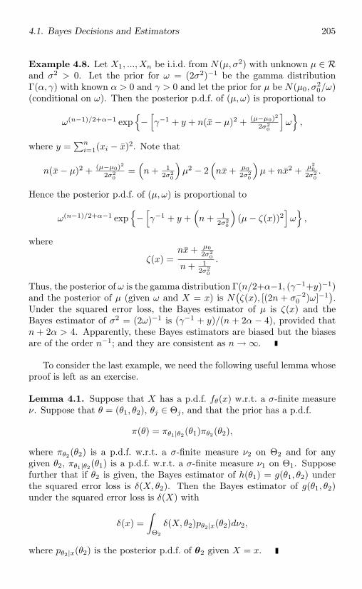
4.1. Bayes Decisions and Estimators 205
Example 4.8. Let X1, ..., Xn be i.i.d. from N(µ, σ2) with unknown µ ∈ Rand σ2 > 0. Let the prior for ω = (2σ2)−1 be the gamma distributionΓ(α, γ) with known α > 0 and γ > 0 and let the prior for µ be N(µ0, σ
20/ω)
(conditional on ω). Then the posterior p.d.f. of (µ, ω) is proportional to
ω(n−1)/2+α−1 exp−
[γ−1 + y + n(x− µ)2 + (µ−µ0)2
2σ20
]ω,
where y =∑n
i=1(xi − x)2. Note that
n(x− µ)2 + (µ−µ0)2
2σ20
=(n + 1
2σ20
)µ2 − 2
(nx + µ0
2σ20
)µ + nx2 + µ2
02σ2
0.
Hence the posterior p.d.f. of (µ, ω) is proportional to
ω(n−1)/2+α−1 exp−
[γ−1 + y +
(n + 1
2σ20
)(µ− ζ(x))2
]ω,
where
ζ(x) =nx + µ0
2σ20
n + 12σ2
0
.
Thus, the posterior of ω is the gamma distribution Γ(n/2+α−1, (γ−1+y)−1)and the posterior of µ (given ω and X = x) is N
(ζ(x), [(2n + σ−2
0 )ω]−1).
Under the squared error loss, the Bayes estimator of µ is ζ(x) and theBayes estimator of σ2 = (2ω)−1 is (γ−1 + y)/(n + 2α − 4), provided thatn + 2α > 4. Apparently, these Bayes estimators are biased but the biasesare of the order n−1; and they are consistent as n → ∞.
To consider the last example, we need the following useful lemma whoseproof is left as an exercise.
Lemma 4.1. Suppose that X has a p.d.f. fθ(x) w.r.t. a σ-finite measureν. Suppose that θ = (θ1, θ2), θj ∈ Θj , and that the prior has a p.d.f.
π(θ) = πθ1|θ2(θ1)πθ2(θ2),
where πθ2(θ2) is a p.d.f. w.r.t. a σ-finite measure ν2 on Θ2 and for anygiven θ2, πθ1|θ2(θ1) is a p.d.f. w.r.t. a σ-finite measure ν1 on Θ1. Supposefurther that if θ2 is given, the Bayes estimator of h(θ1) = g(θ1, θ2) underthe squared error loss is δ(X, θ2). Then the Bayes estimator of g(θ1, θ2)under the squared error loss is δ(X) with
δ(x) =∫
Θ2
δ(X, θ2)pθ2|x(θ2)dν2,
where pθ2|x(θ2) is the posterior p.d.f. of θ2 given X = x.
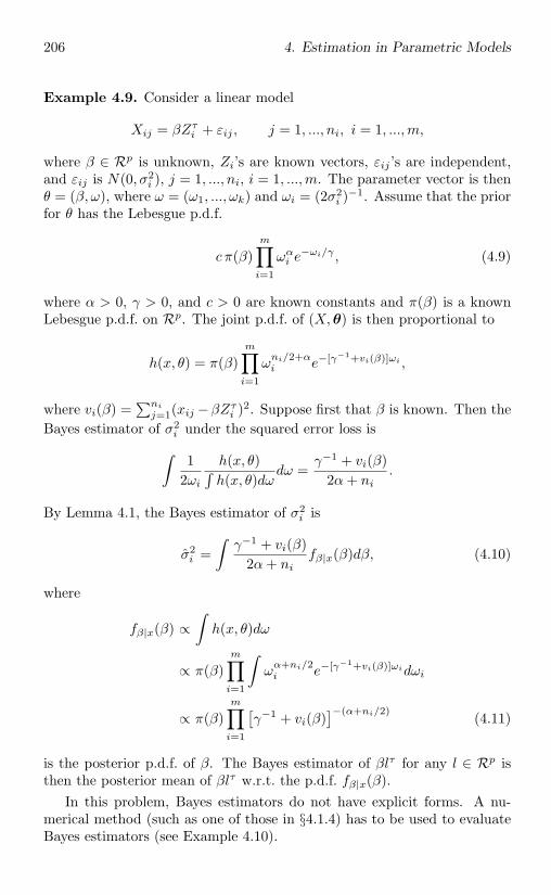
206 4. Estimation in Parametric Models
Example 4.9. Consider a linear model
Xij = βZτi + εij , j = 1, ..., ni, i = 1, ...,m,
where β ∈ Rp is unknown, Zi’s are known vectors, εij ’s are independent,and εij is N(0, σ2
i ), j = 1, ..., ni, i = 1, ...,m. The parameter vector is thenθ = (β, ω), where ω = (ω1, ..., ωk) and ωi = (2σ2
i )−1. Assume that the prior
for θ has the Lebesgue p.d.f.
c π(β)m∏i=1
ωαi e
−ωi/γ , (4.9)
where α > 0, γ > 0, and c > 0 are known constants and π(β) is a knownLebesgue p.d.f. on Rp. The joint p.d.f. of (X,θ) is then proportional to
h(x, θ) = π(β)m∏i=1
ωni/2+αi e−[γ−1+vi(β)]ωi ,
where vi(β) =∑ni
j=1(xij −βZτi )2. Suppose first that β is known. Then the
Bayes estimator of σ2i under the squared error loss is∫
12ωi
h(x, θ)∫h(x, θ)dω
dω =γ−1 + vi(β)
2α + ni.
By Lemma 4.1, the Bayes estimator of σ2i is
σ2i =
∫γ−1 + vi(β)
2α + nifβ|x(β)dβ, (4.10)
where
fβ|x(β) ∝∫
h(x, θ)dω
∝ π(β)m∏i=1
∫ωα+ni/2i e−[γ−1+vi(β)]ωidωi
∝ π(β)m∏i=1
[γ−1 + vi(β)
]−(α+ni/2) (4.11)
is the posterior p.d.f. of β. The Bayes estimator of βlτ for any l ∈ Rp isthen the posterior mean of βlτ w.r.t. the p.d.f. fβ|x(β).
In this problem, Bayes estimators do not have explicit forms. A nu-merical method (such as one of those in §4.1.4) has to be used to evaluateBayes estimators (see Example 4.10).
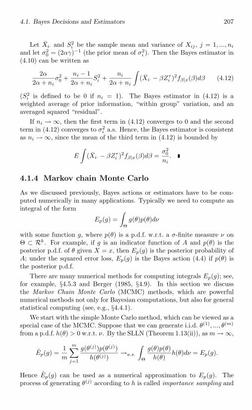
4.1. Bayes Decisions and Estimators 207
Let Xi· and S2i be the sample mean and variance of Xij , j = 1, ..., ni
and let σ20 = (2αγ)−1 (the prior mean of σ2
i ). Then the Bayes estimator in(4.10) can be written as
2α2α + ni
σ20 +
ni − 12α + ni
S2i +
ni
2α + ni
∫(Xi· − βZτ
i )2fβ|x(β)dβ (4.12)
(S2i is defined to be 0 if ni = 1). The Bayes estimator in (4.12) is a
weighted average of prior information, “within group” variation, and anaveraged squared “residual”.
If ni → ∞, then the first term in (4.12) converges to 0 and the secondterm in (4.12) converges to σ2
i a.s. Hence, the Bayes estimator is consistentas ni → ∞, since the mean of the third term in (4.12) is bounded by
E
∫(Xi· − βZτ
i )2fβ|x(β)dβ =σ2
0
ni.
4.1.4 Markov chain Monte Carlo
As we discussed previously, Bayes actions or estimators have to be com-puted numerically in many applications. Typically we need to compute anintegral of the form
Ep(g) =∫
Θg(θ)p(θ)dν
with some function g, where p(θ) is a p.d.f. w.r.t. a σ-finite measure ν onΘ ⊂ Rk. For example, if g is an indicator function of A and p(θ) is theposterior p.d.f. of θ given X = x, then Ep(g) is the posterior probability ofA; under the squared error loss, Ep(g) is the Bayes action (4.4) if p(θ) isthe posterior p.d.f.
There are many numerical methods for computing integrals Ep(g); see,for example, §4.5.3 and Berger (1985, §4.9). In this section we discussthe Markov Chain Monte Carlo (MCMC) methods, which are powerfulnumerical methods not only for Bayesian computations, but also for generalstatistical computing (see, e.g., §4.4.1).
We start with the simple Monte Carlo method, which can be viewed as aspecial case of the MCMC. Suppose that we can generate i.i.d. θ(1), ..., θ(m)
from a p.d.f. h(θ) > 0 w.r.t. ν. By the SLLN (Theorem 1.13(ii)), as m → ∞,
Ep(g) =1m
m∑j=1
g(θ(j))p(θ(j))h(θ(j))
→a.s.
∫Θ
g(θ)p(θ)h(θ)
h(θ)dν = Ep(g).
Hence Ep(g) can be used as a numerical approximation to Ep(g). Theprocess of generating θ(j) according to h is called importance sampling and
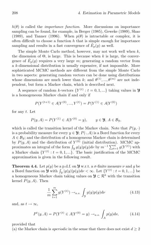
208 4. Estimation in Parametric Models
h(θ) is called the importance function. More discussions on importancesampling can be found, for example, in Berger (1985), Geweke (1989), Shao(1989), and Tanner (1996). When p(θ) is intractable or complex, it isoften difficult to choose a function h that is simple enough for importancesampling and results in a fast convergence of Ep(g) as well.
The simple Monte Carlo method, however, may not work well when k,the dimension of Θ, is large. This is because when k is large, the conver-gence of Ep(g) requires a very large m; generating a random vector froma k-dimensional distribution is usually expensive, if not impossible. Moresophisticated MCMC methods are different from the simple Monte Carloin two aspects: generating random vectors can be done using distributionswhose dimensions are much lower than k; and θ(1), ..., θ(m) are not inde-pendent, but form a Markov chain, which is described next.
A sequence of random k-vectors Y (t) : t = 0, 1, ... taking values in Y
is a homogeneous Markov chain if and only if
P (Y (t+1) ∈ A|Y (0), ..., Y (t)) = P (Y (1) ∈ A|Y (0))
for any t. Let
P (y,A) = P (Y (1) ∈ A|Y (0) = y), y ∈ Y, A ∈ BY,
which is called the transition kernel of the Markov chain. Note that P (y, ·)is a probability measure for every y ∈ Y; P (·, A) is a Borel function for everyA ∈ BY; and the distribution of a homogeneous Markov chain is determinedby P (y,A) and the distribution of Y (0) (initial distribution). MCMC ap-proximates an integral of the form
∫Yg(y)p(y)dν by m−1 ∑m
t=1 g(Y(t)) with
a Markov chain Y (t) : t = 0, 1, .... The basic justification of the MCMCapproximation is given in the following result.
Theorem 4.4. Let p(y) be a p.d.f. on Y w.r.t. a σ-finite measure ν and g bea Borel function on Y with
∫Y|g(y)|p(y)dν < ∞. Let Y (t) : t = 0, 1, ... be
a homogeneous Markov chain taking values on Y ⊂ Rk with the transitionkernel P (y,A). Then
1m
m∑t=1
g(Y (t)) →a.s.
∫Y
g(y)p(y)dν (4.13)
and, as t → ∞,
P t(y,A) = P (Y (t) ∈ A|Y (0) = y) →a.s.
∫A
p(y)dν, (4.14)
provided that(a) the Markov chain is aperiodic in the sense that there does not exist d ≥ 2
4.1. Bayes Decisions and Estimators 209
nonempty disjoint events A0, ..., Ad−1 in BY such that for all i = 0, ..., d− 1and all y ∈ Y, P (y,Aj) = 1 for j = i + 1 (mod d);(b) the Markov chain is p-invariant in the sense that
∫P (y,A)p(y)dν =∫
Ap(y)dν for all A ∈ BY;
(c) the Markov chain is p-irreducible in the sense that for any y ∈ Y and anyA with
∫Ap(y)dν > 0, there exists a positive integer t such that P t(y,A)
in (4.14) is positive; and(d) the Markov chain is Harris recurrent in the sense that for any A with∫Ap(y)dν > 0, P
(∑∞t=1 IA(Y (t)) = ∞|Y (0) = y
)= 1 for all y.
The proof of these results is beyond the scope of this book and, hence, isomitted. It can be found in, for example, Nummelin (1984), Chan (1993),and Tierney (1994). A homogeneous Markov chain satisfying conditions(a)-(d) in Theorem 4.4 is called ergodic with equilibrium distribution p.Result (4.13) means that the MCMC approximation is consistent and result(4.14) indicates that p is the limit p.d.f. of the Markov chain.
One of the key issues in MCMC is the choice of the kernel P (y,A). Thefirst requirement on P (y,A) is that conditions (a)-(d) in Theorem 4.4 aresatisfied. Condition (a) is usually easy to check for any given P (y,A). Inthe following we consider two popular MCMC methods satisfying conditions(a)-(d).
Gibbs sampler
One way to construct a p-invariant homogeneous Markov chain is to useconditioning. Suppose that Y has the p.d.f. p(y). Let Yi (or yi) be the ithcomponent of Y (or y) and let Y−i (or y−i) be the (k−1)-vector containingall components of Y (or y) except Yi (or yi). Then
Pi(y,A) = Pi(y−i, A) = P (Y ∈ A|Y−i = y−i)
is a transition kernel for any i. The MCMC method using this kernel iscalled the single-site Gibbs sampler. Note that∫
Pi(y−i, A)p(y)dν = E[P (Y ∈ A|Y−i)] = P (Y ∈ A) =∫A
p(y)dν
and, therefore, the chain with kernel Pi(y−i, A) is p-invariant. However,this chain is not p-irreducible since P (y−i, ·) puts all its mass on the setψ−1i (y−i), where ψi(y) = y−i. Gelfand and Smith (1990) considered a sys-
tematic scan Gibbs sampler whose kernel P (y,A) is a composite of k kernelsPi(y−i, A), i = 1, ..., k. More precisely, the chain is defined as follows. GivenY (t−1) = y(t−1), we generate y
(t)1 from P1(y
(t−1)2 , ..., y
(t−1)k , · ),..., y(t)
j from
Pj(y(t)1 , ..., y
(t)j−1, y
(t−1)j+1 , ..., y
(t−1)k , · ),..., y
(t)k from Pk(y
(t)1 , ..., y
(t)k−1, · ). The
210 4. Estimation in Parametric Models
initial Y (0) is generated from p. It can be shown that this Markov chainis still p-invariant. We illustrate this with the case of k = 2. Note thatY
(1)1 is generated from P2(y
(0)2 , ·), the conditional distribution of Y given
Y2 = y(0)2 . Hence (Y (1)
1 , Y(0)2 ) has p.d.f. p. Similarly, we can show that
Y (1) = (Y (1)1 , Y
(1)2 ) has p.d.f. p. Thus,∫P (y,A)p(y)dν =
∫P (Y (1) ∈ A|Y (0) = y)p(y)dν
= E[P (Y (1) ∈ A|Y (0))]= P (Y (1) ∈ A)
=∫A
p(y)dν.
This Markov chain is also p-irreducible and aperiodic if p(y) > 0 for ally ∈ Y; see, for example, Chan (1993). Finally, if p(y) > 0 for all y ∈ Y,then P (y,A) the distribution with p.d.f. p for all y and, by Corollary 1of Tierney (1994), the Markov chain is Harris recurrent. Thus, Theorem4.4 applies and (4.13) and (4.14) hold.
The previous Gibbs sampler can obviously be extended to the case whereyi’s are subvectors (of possibly different dimensions) of y.
Let us now return to Bayesian computation and consider the followingexample.
Example 4.10. Consider Example 4.9. Under the given prior for θ =(β, ω), it is difficult to generate random vectors directly from the posteriorp.d.f. p(θ), given X = x (which does not have a familiar form). To apply aGibbs sampler with y = θ, y1 = β, and y2 = ω, we need to generate randomvectors from the posterior of β, given x and ω, and the posterior of ω, givenx and β. From (4.9) and (4.11), the posterior of ω = (ω1, ..., ωk), given xand β, is a product of marginals of ωi’s that are the gamma distributionsΓ(α + 1 + ni/2, [γ−1 + vi(β)]−1), i = 1, ...,m. Assume now that π(β) ≡ 1(noninformative prior for β). It follows from (4.9) that the posterior p.d.f.of β, given x and ω, is proportional to
k∏i=1
e−ωivi(β) ∝ e−‖βZτW 1/2−XW 1/2‖2,
where W is the diagonal matrix whose ith diagonal is ωi. Thus, the poste-rior of βZτW 1/2, given x and ω, is Np(XW 1/2, 2−1Ip) and the posterior ofβ, given x and ω, is Np(XWZ(ZτWZ)−1, 2−1(ZτWZ)−1) (ZτWZ is as-sumed of full rank for simplicity), since β = βZτW 1/2[W 1/2Z(ZτWZ)−1].Note that random generation using these two posterior distributions is fairlyeasy.
4.1. Bayes Decisions and Estimators 211
The Metropolis algorithm
A large class of MCMC methods are obtained using the Metropolis al-gorithm (Metropolis et al., 1953). We introduce Hastings’ version of thealgorithm. Let Q(y,A) be a transition kernel of a homogeneous Markovchain satisfying
Q(y,A) =∫A
q(y, z)dν(z)
for a measurable function q(y, z) ≥ 0 on Y × Y and a σ-finite measure ν.Without loss of generality, assume that
∫Yp(y)dν = 1 and that p is not
concentrated on a single point. Define
α(y, z) =
min
[p(z)q(z,y)p(y)q(y,z) , 1
]p(y)q(y, z) > 0
1 p(y)q(y, z) = 0
and
p(y, z) =
q(y, z)α(y, z) y = z
0 y = z.
The Metropolis kernel P (y,A) is defined by
P (y,A) =∫A
p(y, z)dν(z) + r(y)δy(A), (4.15)
where δy is the point mass at y and r(y) = 1 −∫p(y, z)dν(z). The corre-
sponding Markov chain can be described as follows. If the chain is currentlyat a point Y (t) = y, then it generates a candidate value z for the next lo-cation Y (t+1) from Q(y, ·). With probability α(y, z) the chain moves toY (t+1) = z. Otherwise, the chain remains at Y (t+1) = y.
Note that this algorithm only depends on p(y) through p(y)/p(z). Thus,it can be used when p(y) is known up to a normalizing constant, which oftenoccurs in Bayesian analysis.
We now show that a Markov chain with a Metropolis kernel P (y,A) isp-invariant. First, by the definition of p(y, z) and α(y, z),
p(y)p(y, z) = p(z)p(z, y)
for any y and z. Then, for any A ∈ BY,∫P (y,A)p(y)dν =
∫ [∫A
p(y, z)dν(z)]p(y)dν(y) +
∫r(y)δy(A)p(y)dν(y)
=∫A
[∫p(y, z)p(y)dν(y)
]dν(z) +
∫A
r(y)p(y)dν(y)
=∫A
[∫p(z, y)p(z)dν(y)
]dν(z) +
∫A
r(y)p(y)dν(y)
212 4. Estimation in Parametric Models
=∫A
[1 − r(z)]p(z)dν(z) +∫A
r(z)p(z)dν(z)
=∫A
p(z)dν(z).
If a Markov chain with a Metropolis kernel defined by (4.15) is p-irreducible and
∫r(y)>0 p(y)dν > 0, then, by the results of Nummelin (1984,
§2.4), the chain is aperiodic; by Corollary 2 of Tierney (1994), the chain isHarris recurrent. Hence, to apply Theorem 4.4 to a Markov chain with aMetropolis kernel, it suffices to show that the chain is p-irreducible.
Lemma 4.2. Suppose that Q(y,A) is the transition kernel of a p-irreducibleMarkov chain and that either q(y, z) > 0 for all y and z or q(y, z) = q(z, y)for all y and z. Then the chain with the Metropolis kernel p(y,A) in (4.15)is p-irreducible.Proof. It can be shown (exercise) that if Q is any transition kernel of ahomogeneous Markov chain, then
Qt(y,A) =∫A
∫· · ·
∫ t∏j=1
q(zn−j+1, zn−j)dν(zn−j), (4.16)
where zn = y, y ∈ Y, and A ∈ BY. Let y ∈ Y, A ∈ BY with∫Ap(z)dν > 0,
and By = z : α(y, z) = 1. If∫A∩Bc
yp(z)dν > 0, then
P (y,A) ≥∫A∩Bc
y
q(y, z)α(y, z)dν(z) =∫A∩Bc
y
q(z, y)p(z)p(y)
dν(z) > 0,
which follows from either q(z, y) > 0 or q(z, y) = q(y, z) > 0 on Bcy. If∫
A∩Bcyp(z)dν = 0, then
∫A∩By
p(z)dν > 0. From the irreducibility of
Q(y,A), there exists a t ≥ 1 such that Qt(y,A ∩ By) > 0. Then, by(4.15) and (4.16),
P t(y,A) ≥ P t(y,A ∩By) ≥ Qt(y,A ∩By) > 0.
Two examples of q(y, z) given by Tierney (1994) are q(y, z) = f(z − y)with a Lebesgue p.d.f. f on Rk, which corresponds to a random walk chain,and q(y, z) = f(z) with a p.d.f. f , which corresponds to an independencechain and is closely related to the importance sampling discussed earlier.
Although the MCMC methods have been used over the last 40 years,the research on the theory of MCMC is still very active. Important top-ics include the choice of the transition kernel for MCMC; the rate of theconvergence in (4.13); the choice of the Monte Carlo size m; and the esti-mation of the errors due to Monte Carlo. See more results and discussionsin Tierney (1994), Basag et al. (1995), Tanner (1996), and their references.
4.2. Invariance 213
4.2 Invariance
The concept of invariance is introduced in §2.3.2 (Definition 2.9). In thissection, we study the best invariant estimators and their properties inone-parameter location families (§4.2.1), in one-parameter scale families(§4.2.2), and in general location-scale families (§4.2.3).
4.2.1 One-parameter location families
Assume that the sample X = (X1, ..., Xn) has a joint distribution Pµ witha Lebesgue p.d.f.
f(x1 − µ, ..., xn − µ), (4.17)
where f is known and µ ∈ R is an unknown location parameter. The p.d.f.in (4.17) is a special case of the general location-scale family in Definition2.3. The family P = Pµ : µ ∈ R is called a one-parameter location familyand is invariant under the location transformations gc(X) = (X1 + c,...,Xn + c), c ∈ R.
We consider the estimation of µ as a statistical decision problem withaction space A = R and loss function L(µ, a). It is natural to considerthe same transformation in the action space, i.e., if Xi is transformed toXi+c, then our action a is transformed to a+c. Consequently, the decisionproblem is invariant under location transformation if and only if
L(µ, a) = L(µ + c, a + c) for all c ∈ R,
which is equivalent toL(µ, a) = L(a− µ) (4.18)
for a Borel function L(·) on R.According to Definition 2.9 (see also Example 2.24), an estimator T
(decision rule) of µ is location invariant if and only if
T (X1 + c, ..., Xn + c) = T (X1, ..., Xn) + c. (4.19)
Many estimators of µ, such as the sample mean and weighted average ofthe order statistics, are location invariant. Let di = xi−xn, Di = Xi−Xn,d = (d1, ..., dn−1), and D = (D1, ..., Dn−1). The following result provides acharacterization of location invariant estimators.
Proposition 4.3. Let T0 be a location invariant estimator of µ. A nec-essary and sufficient condition for an estimator T to be location invariantis that there exists a Borel function u on Rn−1 (u ≡ a constant if n = 1)such that
T (x) = T0(x) − u(d) for all x ∈ Rn. (4.20)
214 4. Estimation in Parametric Models
Proof. It is easy to see that T given by (4.20) satisfies (4.19) and, therefore,is location invariant. Suppose that T is location invariant. Let u(x) =T (x) − T0(x) for any x ∈ Rn. Then
u(x1 + c, ..., xn + c) = T (x1 + c, ..., xn + c) − T0(x1 + c, ..., xn + c)= T (x1, ..., xn) − T0(x1, ..., xn)= u(x1, ..., xn)
for all c ∈ R and xi ∈ R. Putting c = −xn leads to
u(d1, ..., dn−1) = u(x1 − xn, ..., xn−1 − xn, 0)= u(x1, ..., xn)= T (x) − T0(x)
for all x ∈ Rn. This proves the result.
The next result states an important property of location invariant esti-mators.
Proposition 4.4. Let X be distributed with the p.d.f. given by (4.17) andlet T be a location invariant estimator of µ under the loss function givenby (4.18). If the bias, variance, and risk of T are well defined, then theyare all constant (do not depend on µ).Proof. The result for the bias follows from
bT (µ) =∫
T (x)f(x1 − µ, ..., xn − µ)dx− µ
=∫
T (x1 + µ, ..., xn + µ)f(x)dx− µ
=∫
[T (x) + µ]f(x)dx− µ
=∫
T (x)f(x)dx.
The proof of the result for variance or risk is left as an exercise.
An important consequence of this result is that the problem of findingthe best location invariant estimator reduces to comparing constants in-stead of risk functions. The following definition can be used not only forlocation invariant estimators, but also for general invariant estimators.
Definition 4.2. Consider an invariant estimation problem in which allinvariant estimators have constant risks. An invariant estimator T is calledthe minimum risk invariant estimator (MRIE) if and only if T has thesmallest risk among all invariant estimators.
4.2. Invariance 215
Theorem 4.5. Let X be distributed with the p.d.f. given by (4.17) andconsider the estimation of µ under the loss function given by (4.18). Sup-pose that there is a location invariant estimator T0 of µ with finite risk.(i) Assume that for each d there exists a u∗(d) that minimizes
E0[L(T0(X) − u(d))|D = d]
over all functions u, where the conditional expectation E0 is calculatedunder the assumption that X has p.d.f. f(x1, ..., xn). Then an MRIE existsand is given by
T∗(X) = T0(X) − u∗(D).
(ii) The function u∗ in (i) exists if L(t) is convex and not monotone; it isunique if L is strictly convex.(iii) If T0 and D are independent, then u∗ is a constant that minimizesE0[L(T0(X)−u)]. If, in addition, the distribution of T0 is symmetric aboutµ and L is convex and even, then u∗ = 0.Proof. By Propositions 4.3 and 4.4,
RT (µ) = EE0[L(T0(x) − u(d))|D = d],
where T (X) = T0(X)−u(D). This proves part (i). If L is (strictly) convexand not monotone, then E0[L(T0(x) − a)|D = d] is (strictly) convex andnot monotone (exercise). Hence lim|a|→∞ E0[L(T0(x) − a)|D = d] = ∞.This proves part (ii). The proof of part (iii) is left as an exercise.
Theorem 4.6. Assume the conditions of Theorem 4.5 and that the loss isthe squared error loss.(i) The unique MRIE of µ is
T∗(X) =
∫ ∞−∞ tf(X1 − t, ..., Xn − t)dt∫ ∞−∞ f(X1 − t, ..., Xn − t)dt
,
which is known as the Pitman estimator of µ.(ii) The MRIE is unbiased.Proof. (i) Under the squared error loss,
u∗(d) = E0[T0(X)|D = d] (4.21)
(exercise). Let T0(X) = Xn (the nth observation). Then Xn is locationinvariant. If there exists a location invariant estimator of µ with finite risk,then E0(Xn|D = d) is finite a.s. P (exercise). By Proposition 1.8, whenµ = 0, the joint Lebesgue p.d.f. of (D,Xn) is f(d1 + xn, ..., dn−1 + xn, xn).The conditional p.d.f. of Xn given D = d is then
f(d1 + xn, ..., dn−1 + xn, xn)∫ ∞−∞ f(d1 + t, ..., dn−1 + t, t)dt
216 4. Estimation in Parametric Models
(see (1.39)). By Proposition 1.11,
E0(Xn|D = d) =
∫ ∞−∞ tf(d1 + t, ..., dn−1 + t, t)dt∫ ∞−∞ f(d1 + t, ..., dn−1 + t, t)dt
=
∫ ∞−∞ tf(x1 − xn + t, ..., xn−1 − xn + t, t)dt∫ ∞−∞ f(x1 − xn + t, ..., xn−1 − xn + t, t)dt
= xn −∫ ∞−∞ uf(x1 − u, ..., xn − u)du∫ ∞−∞ f(x1 − u, ..., xn − u)du
by letting u = xn−t. The result in (i) follows from T∗(X) = Xn−E(Xn|D)(Theorem 4.5).(ii) Let b be the constant bias of T∗ (Proposition 4.4). Then T1(X) =T∗(X) − b is a location invariant estimator of µ and
RT1 = E[T∗(X) − b− µ]2 = Var(T∗) ≤ Var(T∗) + b2 = RT∗ .
Since T∗ is the MRIE, b = 0, i.e., T∗ is unbiased.
Theorem 4.6(ii) indicates that we only need to consider the unbiasedlocation invariant estimator in order to find the MRIE, if the loss is thesquared error loss. In particular, a location invariant UMVUE is an MRIE.
Example 4.11. Let X1, ..., Xn be i.i.d. from N(µ, σ2) with an unknownµ ∈ R and a known σ2. Note that X is location invariant. Since X is theUMVUE of µ (§2.1), it is the MRIE under the squared error loss. Since thedistribution of X is symmetric about µ and X is independent of D (Basu’stheorem), it follows from Theorem 4.5(iii) that X is an MRIE if L is convexand even.
Example 4.12. Let X1, ..., Xn be i.i.d. from the exponential distributionE(µ, θ), where θ is known and µ ∈ R is unknown. Since X(1) − θ/n islocation invariant and is the UMVUE of µ, it is the MRIE under the squarederror loss. Note that X(1) is independent of D (Basu’s theorem). ByTheorem 4.4(iii), an MRIE is of the form X(1) − u∗ with a constant u∗.For the absolute error loss, X(1) − θ log 2/n is an MRIE (exercise).
Example 4.13. Let X1, ..., Xn be i.i.d. from the uniform distribution on(µ − 1
2 , µ + 12 ) with an unknown µ ∈ R. Consider the squared error loss.
Note that
f(x1 − µ, ..., xn − µ) =
1 µ− 12 ≤ x(1) ≤ x(n) ≤ µ + 1
20 otherwise.
4.2. Invariance 217
By Theorem 4.6(i), the MRIE of µ is
T∗(X) =∫ X(1)+ 1
2
X(n)− 12
tdt
/∫ X(1)+ 12
X(n)− 12
dt =X(1) + X(n)
2.
We end this section with a brief discussion of the admissibility of MRIE’sin a one-parameter location problem. Under the squared error loss, theMRIE (Pitman’s estimator) is admissible if there exists a location invariantestimator T0 with E|T0(X)|3 < ∞ (Stein, 1959). Under a general lossfunction, an MRIE is admissible when it is a unique MRIE (under someother minor conditions). See Farrell (1964), Brown (1966), and Brown andFox (1974) for further discussions.
4.2.2 One-parameter scale families
Assume that the sample X = (X1, ..., Xn) has a joint distribution Pσ witha Lebesgue p.d.f.
1σn f
(x1σ , ..., xn
σ
), (4.22)
where f is known and σ > 0 is an unknown scale parameter. The familyP = Pσ : σ > 0 is called a one-parameter scale family and is a specialcase of the general location-scale family in Definition 2.3. This family isinvariant under the scale transformations gr(X) = rX, r > 0.
We consider the estimation of σh with A = [0,∞), where h is a nonzeroconstant. The transformation gr induces the transformation gr(σh) = rhσh.Hence a loss function L is scale invariant if and only if
L(rσ, rha) = L(σ, a) for all r > 0,
which is equivalent toL(σ, a) = L
(aσh
)(4.23)
for a Borel function L(·) on [0,∞). An example of a loss function satisfying(4.23) is
L(σ, a) =∣∣∣∣ a
σh− 1
∣∣∣∣p =|a− σh|p
σph, (4.24)
where p ≥ 1 is a constant. However, the squared error loss does not satisfy(4.23).
An estimator T of σh is scale invariant if and only if
T (rX1, ..., rXn) = rhT (X1, ..., Xn).
Examples of scale invariant estimators are the sample variance S2 (for h =2), the sample standard deviation S =
√S2 (for h = 1), the sample range
218 4. Estimation in Parametric Models
X(n) −X(1) (for h = 1), and the sample mean deviation n−1 ∑ni=1 |Xi− X|
(for h = 1).The following result is an analogue of Proposition 4.3. Its proof is left
as an exercise.
Proposition 4.5. Let T0 be a scale invariant estimator of σh. A necessaryand sufficient condition for an estimator T to be scale invariant is that thereexists a positive Borel function u on Rn such that
T (x) = T0(x)/u(z) for all x ∈ Rn,
where z = (z1, ..., zn), zi = xi/xn, i = 1, ..., n− 1, and zn = xn/|xn|.
The next result is similar to Proposition 4.4. It applies to any invariantproblem defined in Definition 2.9. We use the notation in Definition 2.9.
Theorem 4.7. Let P be a location-scale family invariant for given C andT . Suppose that the loss function is invariant and T is an invariant decisionrule. Then the risk function of T is a constant.
The proof is left as an exercise. Note that a special case of Theorem 4.7is that any scale invariant estimator of σh has a constant risk and, therefore,an MRIE (Definition 4.2) of σh usually exists. However, Proposition 4.4 isnot a special case of Theorem 4.7, since the bias of T may not be a constantin general. For example, the bias of the sample standard deviation is afunction of σ.
The next result and its proof are analogues of those of Theorem 4.5.
Theorem 4.8. Let X be distributed with the p.d.f. given by (4.22) andconsider the estimation of σh under the loss function given by (4.23). Sup-pose that there is a scale invariant estimator T0 of σh with finite risk.(i) Assume that for each z there exists a u∗(z) that minimizes
E1[L(T0(X)/u(z))|Z = z]
over all positive functions u, where the conditional expectation E1 is calcu-lated under the assumption that X has p.d.f. f(x1, ..., xn). Then an MRIEexists and is given by
T∗(X) = T0(X)/u∗(Z).
(ii) The function u∗ in (i) exists if γ(t) = L(et) is convex and not monotone;it is unique if γ(t) is strictly convex.
The loss function given by (4.24) satisfies the condition in Theorem4.8(ii). A loss function corresponding to the squared error loss in this
4.2. Invariance 219
problem is the loss function (4.24) with p = 2. We have the following resultsimilar to Theorem 4.6 (its proof is left as an exercise).
Corollary 4.1. Under the conditions of Theorem 4.8 and the loss function(4.24) with p = 2, the unique MRIE of σh is
T∗(X) =T0(X)E1[T0(X)|Z]E1[T0(X)]2|Z =
∫ ∞0 tn+h−1f(tX1, ..., tXn)dt∫ ∞0 tn+2h−1f(tX1, ..., tXn)dt
,
which is known as the Pitman estimator of σh.
Example 4.14. Let X1, ..., Xn be i.i.d. from N(0, σ2) and consider the es-timation of σ2. Then T0 =
∑ni=1 X
2i is scale invariant. By Basu’s theorem,
T0 is independent of Z. Hence u∗ in Theorem 4.8 is a constant minimizingE1[L(T0/u)] over u > 0. When the loss is given by (4.24) with p = 2, byCorollary 4.1, the MRIE (Pitman’s estimator) is
T∗(X) =T0(X)E1[T0(X)]
E1[T0(X)]2=
1n + 2
n∑i=1
X2i ,
since T0 has a chi-square distribution χ2n when σ = 1. Note that the
UMVUE of σ2 is T0/n, which is different from the MRIE.
Example 4.15. Let X1, ..., Xn be i.i.d. from the uniform distribution on(0, σ) and consider the estimation of σ. By Basu’s theorem, the scale in-variant estimator X(n) is independent of Z. Hence u∗ in Theorem 4.8 is aconstant minimizing E1[L(X(n)/u)] over u > 0. When the loss is given by(4.24) with p = 2, by Corollary 4.1, the MRIE (Pitman’s estimator) is
T∗(X) =X(n)E1X(n)
E1X2(n)
=(n + 2)X(n)
n + 1.
4.2.3 General location-scale families
Assume that X = (X1, ..., Xn) has a joint distribution Pθ with a Lebesguep.d.f.
1σn f
(x1−µ
σ , ..., xn−µσ
), (4.25)
where f is known, θ = (µ, σ) ∈ Θ, and Θ = R × (0,∞). The familyP = Pθ : θ ∈ Θ is a special case of the location-scale family definedin Definition 2.3 and is invariant under the location-scale transformationsgc,r(X) = (rX1 + c, ..., rXn + c), c ∈ R, r > 0, which induce similartransformations on Θ: gc,r(θ) = (rµ + c, rσ), c ∈ R, r > 0.
220 4. Estimation in Parametric Models
Consider the estimation of σh with a fixed h = 0 under the loss function(4.23), which is invariant under the location-scale transformations gc,r. Anestimator T of σh is location-scale invariant if and only if
T (rX1 + c, ..., rXn + c) = rhT (X1, ..., Xn). (4.26)
By Theorem 4.7, any location-scale invariant T has a constant risk. Lettingr = 1 in (4.26), we obtain that
T (X1 + c, ..., Xn + c) = T (X1, ..., Xn)
for all c ∈ R. Therefore, T is a function of D = (D1, ..., Dn−1), Di =Xi −Xn, i = 1, ..., n− 1. From (4.25), the joint Lebesgue p.d.f. of D is
1σn−1
∫ ∞−∞ f
(d1σ + t, ..., dn−1
σ + t, t)dt, (4.27)
which is of the form (4.22) with n replaced by n−1 and xi’s replaced by di’s.It follows from Theorem 4.8 that if T0(D) is any finite risk scale invariantestimator of σh based on D, then an MRIE of σh is
T∗(D) = T0(D)/u∗(W ), (4.28)
where W = (W1, ...,Wn−1), Wi = Di/Dn−1, i = 1, ..., n − 2, Wn−1 =Dn−1/|Dn−1|, u∗(w) is any number minimizing E1[L(T0(D)/u(w))|W = w]over all positive functions u, and E1 is the conditional expectation calcu-lated under the assumption that D has p.d.f. (4.27) with σ = 1.
Consider next the estimation of µ. Under the location-scale transfor-mation gc,r, it can be shown (exercise) that a loss function is invariant ifand only if it is of the form
L(a−µσ
). (4.29)
An estimator T of µ is location-scale invariant if and only if
T (rX1 + c, ..., rXn + c) = rT (X1, ..., Xn) + c.
Again, by Theorem 4.7, the risk of an invariant T is a constant.The following result is an analogue of Proposition 4.3 or 4.5.
Proposition 4.6. Let T0 be any estimator of µ invariant under location-scale transformation and let T1 be any estimator of σ satisfying (4.26) withh = 1 and T1 > 0. Then an estimator T of µ is location-scale invariant ifand only if there is a Borel function u on Rn−1 such that
T (X) = T0(X) − u(W )T1(X),
where W is given in (4.28).
4.2. Invariance 221
The proofs of Proposition 4.6 and the next result, an analogue of The-orem 4.4 or 4.7, are left as exercises.
Theorem 4.9. Let X be distributed with p.d.f. given by (4.25) and con-sider the estimation of µ under the loss function given by (4.29). Supposethat there exist finite risk location-scale invariant estimators T0 of µ andT1 of σ. Then an MRIE of µ is
T∗(X) = T0(X) − u∗(W )T1(X),
where W is given in (4.28), u∗(w) is any number minimizing
E0,1[L(T0(X) − u(w)T1(X))|W = w]
over all functions u, and E0,1 is computed under the assumption that Xhas the p.d.f. (4.25) with µ = 0 and σ = 1.
Corollary 4.2. Under the conditions of Theorem 4.9 and the loss function(a− µ)2/σ2, u∗(w) in Theorem 4.9 is equal to
u∗(w) =E0,1[T0(X)T1(X)|W = w]E0,1[T1(X)]2|W = w .
Example 4.16. Let X1, ..., Xn be i.i.d. from N(µ, σ2), where µ ∈ R andσ2 > 0 are unknown. Consider first the estimation of σ2 under loss function(4.23). The sample variance S2 is location-scale invariant and is indepen-dent of W in (4.28) (Basu’s theorem). Thus, by (4.28), S2/u∗ is an MRIE,where u∗ is a constant minimizing E1[L(S2/u)] over all u > 0. If the lossfunction is given by (4.24) with p = 2, then by Corollary 4.1, the MRIE ofσ2 is
T∗(X) =S2E1(S2)E1(S2)2
=S2
(n2 − 1)/(n− 1)2=
1n + 1
n∑i=1
(Xi − X)2,
since (n− 1)S2 has a chi-square distribution χ2n−1 when σ = 1.
Next, consider the estimation of µ under the loss function (4.29). SinceX is a location-scale invariant estimator of µ and is independent of W in(4.28) (Basu’s theorem), by Theorem 4.9, an MRIE of µ is
T∗(X) = X − u∗S2,
where u∗ is a constant. If L in (4.29) is convex and even, then u∗ = 0 (seeTheorem 4.5(iii)) and, hence, X is an MRIE of µ.
Example 4.17. Let X1, ..., Xn be i.i.d. from the uniform distribution on(µ− 1
2σ, µ + 12σ), where µ ∈ R and σ > 0 are unknown. Consider first the
222 4. Estimation in Parametric Models
estimation of σ under the loss function (4.24) with p = 2. The sample rangeX(n) −X(1) is a location-scale invariant estimator of σ and is independentof W in (4.28) (Basu’s theorem). By (4.28) and Corollary 4.1, the MRIEof σ is
T∗(X) =(X(n) −X(1))E1(X(n) −X(1))
E1(X(n) −X(1))2=
(n + 2)(X(n) −X(1))n
.
Consider now the estimation of µ under the loss function (4.29). Since(X(1) + X(n))/2 is a location-scale invariant estimator of µ and is inde-pendent of W in (4.28) (Basu’s theorem), by Theorem 4.9, an MRIE of µis
T∗(X) =X(1) + X(n)
2− u∗(X(n) −X(1)),
where u∗ is a constant. If L in (4.29) is convex and even, then u∗ = 0 (seeTheorem 4.5(iii)) and, hence, (X(1) + X(n))/2 is an MRIE of µ.
Finding MRIE’s in various subfamilies of the location-scale family inDefinition 2.3 under transformations XA + c, where A ∈ T and c ∈ Cwith given T and C, can be done in a similar way. We only provide somebrief discussions for two important cases. The first case is the two-samplelocation-scale problem in which two samples, X = (X1, ..., Xm) and Y =(Y1, ..., Yn), are taken from a distribution with Lebesgue p.d.f.
1σmx σn
yf(
x1−µx
σx, ..., xm−µx
σx,y1−µy
σy, ...,
yn−µy
σy
), (4.30)
where f is known, µx ∈ R and µy ∈ R are unknown location parameters,and σx > 0 and σy > 0 are unknown scale parameters. The family ofdistributions is invariant under the transformations
g(X,Y ) = (rX1 + c, ..., rXm + c, r′Y1 + c′, ..., r′Yn + c′), (4.31)
where r > 0, r′ > 0, c ∈ R, and c′ ∈ R. The parameters to be estimatedin this problem are usually ∆ = µy − µx and η = (σy/σx)h with a fixedh = 0. If X and Y are from two populations, ∆ and η are measures of thedifference between the two populations. For estimating η, results similar tothose in this section can be established. For estimating ∆, MRIE’s can beobtained under some conditions. See Exercises 54-56.
The second case is the general linear model (3.25) under the assumptionthat εi’s are i.i.d. with the p.d.f. σ−1f(x/σ), where f is a known Lebesguep.d.f. The family of populations is invariant under the transformations
g(X) = rX + cZτ , r ∈ (0,∞), c ∈ Rp (4.32)
4.3. Minimaxity and Admissibility 223
(exercise). The estimation of βlτ with l ∈ R(Z) is invariant under theloss function L
(a−βlτ
σ
)and the LSE βlτ is an invariant estimator of βlτ
(exercise). When f is normal, the following result can be established usingan argument similar to that in Example 4.16.
Theorem 4.10. Consider model (3.25) with assumption A1.(i) Under transformations (4.32) and the loss function L
(a−βlτ
σ
), where L
is convex and even, the LSE βlτ is an MRIE of βlτ for any l ∈ R(Z).(ii) Under transformations (4.32) and the loss function (a − σ2)2/σ4, theMRIE of σ2 is SSR/(n− q + 2), where SSR is given by (3.36) and q is therank of Z.
MRIE’s in a parametric family with a multi-dimensional θ are ofteninadmissible. See Lehmann (1983, p. 285) for more discussions.
4.3 Minimaxity and Admissibility
Consider the estimation of a real-valued ϑ = g(θ) based on a sample X fromPθ, θ ∈ Θ, under a given loss function. A minimax estimator minimizes themaximum risk supθ∈Θ RT (θ) over all estimators T (see §2.3.2).
A unique minimax estimator is admissible, since any estimator betterthan a minimax estimator is also minimax. This indicates that we shouldconsider minimaxity and admissibility together. The situation is differentfor a UMVUE (or an MRIE), since if a UMVUE (or an MRIE) is inadmis-sible, it is dominated by an estimator that is not unbiased (or invariant).
4.3.1 Estimators with constant risks
By minimizing the maximum risk, a minimax estimator tries to do as wellas possible in the worst case. Such an estimator can be very unsatisfactory.However, if a minimax estimator has some other good properties (e.g., it isa Bayes estimator), then it is often a reasonable estimator. Here we studywhen estimators having constant risks (e.g., MRIE’s) are minimax.
Theorem 4.11. Let Π be a proper prior on Θ and δ be a Bayes estimatorof ϑ w.r.t. Π. Let ΘΠ = θ : Rδ(θ) = supθ∈Θ Rδ(θ). If Π(ΘΠ) = 1, then δis minimax. If, in addition, δ is the unique Bayes estimator w.r.t. Π, thenit is the unique minimax estimator.Proof. Let T be any other estimator of ϑ. Then
supθ∈Θ
RT (θ) ≥∫
ΘΠ
RT (θ)dΠ ≥∫
ΘΠ
Rδ(θ)dΠ = supθ∈Θ
Rδ(θ).
224 4. Estimation in Parametric Models
If δ is the unique Bayes estimator, then the second inequality in the previousexpression should be replaced by > and, therefore, δ is the unique minimaxestimator.
The condition of Theorem 4.11 essentially means that δ has a constantrisk. Thus, a Bayes estimator having constant risk is minimax.
Example 4.18. Let X1, ..., Xn be i.i.d. binary random variables withP (X1 = 1) = p ∈ (0, 1). Consider the estimation of p under the squared er-ror loss. The UMVUE X has risk p(1−p)/n which is not constant. In fact,X is not minimax (Exercise 58). To find a minimax estimator by applyingTheorem 4.11, we consider the Bayes estimator w.r.t. the beta distributionB(α, β) with known α and β (Exercise 1):
δ(X) = (α + nX)/(α + β + n).
A straightforward calculation shows that
Rδ(p) = [np(1 − p) + (α− αp− βp)2]/(α + β + n)2.
To apply Theorem 4.11, we need to find values of α > 0 and β > 0 suchthat Rδ(p) is constant. It can be shown that Rδ(p) is constant if and onlyif α = β =
√n/2, which leads to the unique minimax estimator
T (X) = (nX +√n/2)
/(n +
√n).
The risk of T is RT = 1/[4(1 +√n)2].
Note that T is a Bayes estimator and has some good properties. Com-paring the risk of T with that of X, we find that T has smaller risk if andonly if
p ∈(
12 − 1
2
√1 − n
(1+√n)2 ,
12 + 1
2
√1 − n
(1+√n)2
). (4.33)
Thus, for small value of n, T is better (and can be much better) than X formost of the range of p (Figure 4.1). When n → ∞, the interval in (4.33)shrinks toward 1
2 . Hence, for large (and even moderate) n, X is betterthan T for most of the range of p (Figure 4.1). The limit of the asymptoticrelative efficiency of T w.r.t. X is 4p(1− p), which is always smaller than 1when p = 1
2 and equals 1 when p = 12 .
The minimax estimator depends strongly on the loss function. To seethis, let us consider the loss function L(p, a) = (a−p)2/[p(1−p)]. Under thisloss function, X has constant risk and is the unique Bayes estimator w.r.t.the uniform prior on (0, 1). By Theorem 4.11, X is the unique minimaxestimator. On the other hand, the risk of T is equal to 1/[4(1+
√n)2p(1−p)],
which is unbounded.
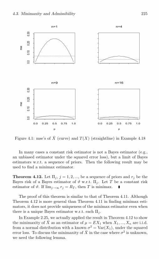
4.3. Minimaxity and Admissibility 225
mse
0.00.1
00.2
00.3
0n=1
n=4
p
mse
0.0 0.25 0.5 0.75 1.0
0.00.1
00.2
00.3
0
n=9
p
0.0 0.25 0.5 0.75 1.0
n=16
Figure 4.1: mse’s of X (curve) and T (X) (straightline) in Example 4.18
In many cases a constant risk estimator is not a Bayes estimator (e.g.,an unbiased estimator under the squared error loss), but a limit of Bayesestimators w.r.t. a sequence of priors. Then the following result may beused to find a minimax estimator.
Theorem 4.12. Let Πj , j = 1, 2, ..., be a sequence of priors and rj be theBayes risk of a Bayes estimator of ϑ w.r.t. Πj . Let T be a constant riskestimator of ϑ. If limj→∞ rj = RT , then T is minimax.
The proof of this theorem is similar to that of Theorem 4.11. AlthoughTheorem 4.12 is more general than Theorem 4.11 in finding minimax esti-mators, it does not provide uniqueness of the minimax estimator even whenthere is a unique Bayes estimator w.r.t. each Πj .
In Example 2.25, we actually applied the result in Theorem 4.12 to showthe minimaxity of X as an estimator of µ = EX1 when X1, ..., Xn are i.i.d.from a normal distribution with a known σ2 = Var(X1), under the squarederror loss. To discuss the minimaxity of X in the case where σ2 is unknown,we need the following lemma.
226 4. Estimation in Parametric Models
Lemma 4.3. Let Θ0 be a subset of Θ and T be a minimax estimator of ϑwhen Θ0 is the parameter space. Then T is a minimax estimator if
supθ∈Θ
RT (θ) = supθ∈Θ0
RT (θ).
Proof. If there is an estimator T0 with supθ∈Θ RT0(θ) < supθ∈Θ RT (θ),then
supθ∈Θ0
RT0(θ) ≤ supθ∈Θ
RT0(θ) < supθ∈Θ
RT (θ) = supθ∈Θ0
RT (θ),
which contradicts the minimaxity of T when Θ0 is the parameter space.Hence, T is minimax when Θ is the parameter space.
Example 4.19. Let X1, ..., Xn be i.i.d. from N(µ, σ2) with unknown θ =(µ, σ2). Consider the estimation of µ under the squared error loss. Supposefirst that Θ = R× (0, c] with a constant c > 0. Let Θ0 = R× c. FromExample 2.25, X is a minimax estimator of µ when the parameter spaceis Θ0. An application of Lemma 4.3 shows that X is also minimax whenthe parameter space is Θ. Although σ2 is assumed to be bounded by c, theminimax estimator X does not depend on c.
Consider next the case where Θ = R × (0,∞), i.e., σ2 is unbounded.Let T be any estimator of µ. For any fixed σ2,
σ2
n≤ sup
µ∈RRT (θ),
since σ2/n is the risk of X which is minimax when σ2 is known (Example2.25). Letting σ2 → ∞, we obtain that supθ RT (θ) = ∞ for any estimatorT . Thus, minimaxity is meaningless (any estimator is minimax).
Theorem 4.13. Suppose that T as an estimator of ϑ has constant risk andis admissible. Then T is minimax. If the loss function is strictly convex,then T is the unique minimax estimator.Proof. By the admissibility of T , if there is another estimator T0 withsupθ RT0(θ) ≤ RT , then RT0(θ) = RT for all θ. This proves that T isminimax. If the loss function is strictly convex and T0 is another minimaxestimator, then
R(T+T0)/2(θ) < (RT0 + RT )/2 = RT
for all θ and, therefore, T is inadmissible. This shows that T is unique ifthe loss is strictly convex.
Combined with Theorem 4.7, Theorem 4.13 tells us that if an MRIE isadmissible, then it is minimax. From the discussion at the end of §4.2.1,MRIE’s in one-parameter location families (such as Pitman’s estimators)are usually minimax.
4.3. Minimaxity and Admissibility 227
4.3.2 Results in one-parameter exponential families
The following result provides a sufficient condition for the admissibility ofa class of estimators when the population Pθ is in a one-parameter expo-nential family. Using this result and Theorem 4.13, we can obtain a classof minimax estimators. The proof of this result is an application of theinformation inequality introduced in §3.1.3.
Theorem 4.14. Suppose that X has the p.d.f. c(θ)eθT (x) w.r.t. a measureν, where T (x) is real-valued and θ ∈ (θ−, θ+) ⊂ R. Consider the estimationof ϑ = E[T (X)] under the squared error loss. Let λ ≥ 0 and γ be knownconstants and let Tλ,γ(X) = (T + γλ)/(1 + λ). Then a sufficient conditionfor the admissibility of Tλ,γ is that∫ θ+
θ0
eγλθ
[c(θ)]λdθ =
∫ θ0
θ−
eγλθ
[c(θ)]λdθ = ∞, (4.34)
where θ0 ∈ (θ−, θ+).Proof. From Theorem 2.1, ϑ = E[T (X)] = −c′(θ)/c(θ) and dϑ
dθ = Var(T )=I(θ), the Fisher information defined in (3.5). Suppose that there is anestimator δ such that for all θ,
Rδ(θ) ≤ RTλ,γ(θ) = [I(θ) + λ2(ϑ− γ)2]/(1 + λ)2.
From the information inequality (3.6),
Rδ(θ) ≥ [bδ(θ)]2 + [I(θ) + b′δ(θ)]2/I(θ).
Let h(θ) = bδ(θ) − λ(γ − ϑ)/(1 + λ). Then
[h(θ)]2 − 2λh(θ)(ϑ− γ) + 2h′(θ)1 + λ
+[h′(θ)]2
I(θ)≤ 0,
which implies
[h(θ)]2 − 2λh(θ)(ϑ− γ) + 2h′(θ)1 + λ
≤ 0. (4.35)
Let a(θ) = h(θ)[c(θ)]λeγλθ. Differentiation of a(θ) reduces (4.35) to
[a(θ)]2e−γλθ
[c(θ)]λ+
2a′(θ)1 + λ
≤ 0. (4.36)
Suppose that a(θ0) < 0 for some θ0 ∈ (θ−, θ+). From (4.36), a′(θ) ≤ 0 forall θ. Hence a(θ) < 0 for all θ ≥ θ0 and, for θ > θ0, (4.36) can be writtenas
d
dθ
[1
a(θ)
]≥ (1 + λ)e−γλθ
2[c(θ)]λ.
228 4. Estimation in Parametric Models
Integrating both sides from θ0 to θ gives
1 + λ
2
∫ θ
θ0
e−γλθ
[c(θ)]λdθ ≤ 1
a(θ)− 1
a(θ0)≤ − 1
a(θ0).
Letting θ → θ+, the left-hand side of the previous expression diverges to ∞by condition (4.34), which is impossible. This shows that a(θ) ≥ 0 for allθ. Similarly, we can show that a(θ) ≤ 0 for all θ. Thus, a(θ) = 0 for all θ.This means that h(θ) = 0 for all θ and the equality in (4.35) holds, whichimplies Rδ(θ) ≡ RTλ,γ
(θ). This proves the admissibility of Tλ,γ .
The reason why Tλ,γ is considered is that it is often a Bayes estimatorw.r.t. some prior; see, for example, Examples 2.25, 4.1, 4.7, and 4.8. Tofind minimax estimators, we may use the following result.
Corollary 4.3. Assume that X has the p.d.f. as described in Theorem4.14 with θ− = −∞ and θ+ = ∞.(i) As an estimator of ϑ = E(T ), T (X) is admissible under the squarederror loss and the loss (a− ϑ)2/Var(T ).(ii) T is the unique minimax estimator of ϑ under the loss (a−ϑ)2/Var(T ).Proof. (i) With λ = 0, condition (4.34) is clearly satisfied. Hence, Theorem4.14 applies under the squared error loss. The admissibility of T under theloss (a − ϑ)2/Var(T ) follows from the fact that T is admissible under thesquared error loss and Var(T ) = 0.(ii) This is a consequence of part (i) and Theorem 4.13.
Example 4.20. Let X1, ..., Xn be i.i.d. from N(0, σ2) with an unknownσ2 > 0. Let Y =
∑ni=1 X
2i . From Example 4.14, Y/(n+2) is the MRIE of σ2
and has constant risk, under the loss (a−σ2)2/σ4. We now apply Theorem4.14 to show that Y/(n+2) is admissible. Note that the joint p.d.f. of Xi’sis of the form c(θ)eθT (x) with θ = −n/(4σ2), c(θ) = (−2θ/n)n/2, T (X) =2Y/n, θ− = −∞, and θ+ = 0. By Theorem 4.14, Tλ,γ(T + γλ)/(1 + λ) isadmissible under the squared error loss if∫ −c
−∞e−γλθ
(−2θn
)−nλ/2
dθ =∫ c
0eγλθθ−nλ/2dθ = ∞
for some c > 0. This means that Tλ,γ is admissible if γ = 0 and λ = 2/n, orif γ > 0 and λ ≥ 2/n. In particular, 2Y/(n+2) is admissible for estimatingE(T ) = 2E(Y )/n = 2σ2, under the squared error loss. It is easy to see thatY/(n + 2) is then an admissible estimator of σ2 under the squared errorloss and the loss (a− σ2)2/σ4. Hence Y/(n + 2) is minimax under the loss(a− σ2)2/σ4.
Note that we cannot apply Corollary 4.3 directly since θ+ = 0.
4.3. Minimaxity and Admissibility 229
Example 4.21. Let X1, ..., Xn be i.i.d. from the Poisson distribution P (θ)with an unknown θ > 0. The joint p.d.f. of Xi’s w.r.t. the counting measureis (x1! · · ·xn!)−1e−nθenx log θ. For η = n log θ, the conditions of Corollary4.3 are satisfied with T (X) = X. Since E(T ) = θ and Var(T ) = θ/n,by Corollary 4.3, X is the unique minimax estimator of θ under the lossfunction (a− θ)2/θ.
4.3.3 Simultaneous estimation and shrinkage estimators
In this chapter (and most of Chapter 3) we have been focused on the es-timation of a real-valued ϑ. The problem of estimating a vector-valuedϑ under the decision theory approach is called simultaneous estimation.Many results for the case of a real-valued ϑ can be extended to simultane-ous estimation in a straightforward manner.
Let ϑ be a p-vector of parameters (functions of θ) with range Θ. Avector-valued estimator T (X) can be viewed as a decision rule taking valuesin the action space A = Θ. Let L(θ, a) be a given nonnegative loss functionon Θ × A. A natural generalization of the squared error loss is
L(θ, a) = ‖a− ϑ‖2 =p∑
i=1
(ai − ϑi)2, (4.37)
where ai and ϑi are the ith components of a and ϑ, respectively.A vector-valued estimator T is called unbiased if and only if E(T ) = ϑ
for all θ ∈ Θ. If there is an unbiased estimator of ϑ, then ϑ is calledestimable. It can be seen that the result in Theorem 3.1 extends to thecase of vector-valued ϑ with any L strictly convex in a. If the loss functionis given by (4.37) and Ti is a UMVUE of ϑi for each i, then T = (T1, ..., Tp)is a UMVUE of ϑ. If there is a sufficient and complete statistic U(X) forθ, then by Theorem 2.5 (Rao-Blackwell’s theorem), T must be a functionof U(X) and is the unique best unbiased estimator of ϑ.
Example 4.22. Consider the general linear model (3.25) with assumptionA1 and a full rank Z. Let ϑ = β. An unbiased estimator of β is then theLSE β. From the proof of Theorem 3.7, β is a function of the sufficient andcomplete statistic for θ = (β, σ2). Hence, β is the unique best unbiasedestimator of ϑ under any strictly convex loss function. In particular, β isthe UMVUE of β under the loss function (4.37).
Next, we consider Bayes estimators of ϑ, which is still defined to beBayes actions considered as functions of X. Under the loss function (4.37),the Bayes estimator is still given by (4.4) with vector-valued g(θ) = ϑ.
230 4. Estimation in Parametric Models
Example 4.23. Let X = (X0, X1, ..., Xk) have the multinomial dis-tribution given in Example 2.7. Consider the estimation of the vectorθ = (p0, p1, ..., pk) under the loss function (4.37), and the Dirichlet priorfor θ which has the Lebesgue p.d.f.
Γ(α0, ..., αk)Γ(α0) · · ·Γ(αk)
pα0−10 · · · pαk−1
k IA(θ), (4.38)
where αj ’s are known positive constants and A = θ : 0 ≤ pj ,∑k
j=0 pj = 1.It turns out that the Dirichlet prior is conjugate so that the posterior of θgiven X = x is also a Dirichlet distribution having the p.d.f. given by (4.38)with αj replaced by αj + xj , j = 0, 1, ..., k. Thus, the Bayes estimator of θis δ = (δ0, δ1, ..., δk) with
δj(X) =αj + Xj
α0 + α1 + · · · + αk + n, j = 0, 1, ..., k.
After a suitable class of transformations is defined, the results in §4.2for invariant estimators and MRIE’s are still valid. This is illustrated bythe following example.
Example 4.24. Let X be a sample with the Lebesgue p.d.f. f(x − θ),where f is a known Lebesgue p.d.f. on Rp with a finite second moment andθ ∈ Rp is an unknown parameter. Consider the estimation of θ under theloss function (4.37). This problem is invariant under the location transfor-mations g(X) = X + c, where c ∈ Rp. Invariant estimators of θ are of theform X + l, l ∈ Rp. It is easy to show that any invariant estimator hasconstant bias and risk (a generalization of Proposition 4.4) and the MRIEof θ is the unbiased invariant estimator. In particular, if f is the p.d.f. ofNp(0, Ip), then the MRIE is X.
The definition of minimax estimators applies without changes.
Example 4.25. Let X be a sample from Np(θ, Ip) with an unknownθ ∈ Rp. Consider the estimation of θ under the loss function (4.37). Amodification of the proof of Theorem 4.12 with independent priors for θi’sshows that X is a minimax estimator of θ (exercise).
Example 4.26. Consider Example 4.23. If we choose α0 = · · · = αk =√n/(k + 1), then the Bayes estimator of θ in Example 4.23 has constant
risk. Using the same argument in the proof of Theorem 4.11, we can showthat this Bayes estimator is minimax.
The previous results for simultaneous estimation are fairly straightfor-ward generalizations of those for the case of real-valued ϑ. Results for
4.3. Minimaxity and Admissibility 231
admissibility in simultaneous estimation, however, are quite different. Asurprising result, due to Stein (1956), is that in estimating the vector meanθ = EX of a normally distributed p-vector X (Example 4.25), X is in-admissible under the loss function (4.37) when p ≥ 3, although X is theUMVUE, MRIE (Example 4.24), and minimax estimator (Example 4.25).Since any estimator better than a minimax estimator is also minimax, thereexist many (in fact, infinitely many) minimax estimators in Example 4.25when p ≥ 3, which is different from the case of p = 1 in which X is theunique admissible minimax estimator (Example 4.6 and Theorem 4.13).
We start with the simple case where X is from Np(θ, Ip) with an un-known θ ∈ Rp. James and Stein (1961) proposed the following class ofestimators of ϑ = θ having smaller risks than X when the loss is given by(4.37) and p ≥ 3:
δc = c +(
1 − p− 2‖X − c‖2
)(X − c), (4.39)
where c ∈ Rp is fixed. The choice of c is discussed next and at the end ofthis section.
Before we prove that δc in (4.39) is better than X, we try to motivateδc from two viewpoints. First, suppose that it were thought a priori likely,though not certain, that θ = c. Then we might first test a hypothesisH0 : θ = c and estimate θ by c if H0 is accepted and by X otherwise. Thebest rejection region has the form ‖X − c‖2 > t for some constant t > 0(see Chapter 6) so that we might estimate θ by
I(t,∞)(‖X − c‖2)X + [1 − I(t,∞)(‖X − c‖2)]c.
It can been seen that δc in (4.39) is a smoothed version of this estimator,since
δc = ψ(‖X − c‖2)X + [1 − ψ(‖X − c‖2)]c (4.40)for some function ψ. Any estimator having the form of the right-hand sideof (4.40) shrinks the observations toward a given point c and, therefore, iscalled a shrinkage estimator.
Next, δc in (4.40) can be viewed as an empirical Bayes estimator (§4.1.2).In view of (2.28) in Example 2.25, a Bayes estimator of θ is of the form
δ = (1 −B)X + Bc,
where c is the prior mean of θ and B involves prior variances. If 1 − B is“estimated” by ψ(‖X − c‖2), then δc is an empirical Bayes estimator.
Theorem 4.15. Suppose that X is from Np(θ, Ip) with p ≥ 3. Then,under the loss function (4.37), the risks of the following estimators of θ,
δc,r = c +[1 − r(p− 2)
‖X − c‖2
](X − c), (4.41)
232 4. Estimation in Parametric Models
are given by
Rδc,r (θ) = p− (2r − r2)(p− 2)2E(‖X − c‖−2), (4.42)
where c ∈ Rp and r ∈ R are known.Proof. Let Z = X − c. Then
Rδc,r (θ) = E‖δc,r − E(X)‖2 = E
∥∥∥∥(1 − p− 2
‖Z‖2
)Z − E(Z)
∥∥∥∥2
.
Hence, we only need to show the case of c = 0. Let h(θ) = Rδ0,r (θ), g(θ) bethe right-hand side of (4.42) with c = 0, and π(θ) = (2πα)−p/2e−‖θ‖2/(2α),which is the p.d.f. of Np(0, αIp). Note that the distribution of X can beviewed as the conditional distribution of X given θ = θ, where θ has theLebesgue p.d.f. π(θ). Then∫
Rp
g(θ)π(θ)dθ = p− (2r − r2)(p− 2)2E[E(‖X‖−2|θ)]
= p− (2r − r2)(p− 2)2E(‖X‖−2)= p− (2r − r2)(p− 2)/(α + 1),
where the expectation in the second line of the previous expression is w.r.t.the joint distribution of (X,θ) and the last equality follows from the factthat the marginal distribution of X is Np(0, (α+1)Ip), ‖X‖2/(α+1) has thechi-square distribution χ2
p and, therefore, E(‖X‖−2) = 1/[(p − 2)(α + 1)].Let B = 1/(α + 1) and B = r(p− 2)/‖X‖2. Then∫
Rp
h(θ)π(θ)dθ = E‖(1 − B)X − θ‖2
= EE[‖(1 − B)X − θ‖2|X]= EE[‖θ − E(θ|X)‖2|X]
+ ‖E(θ|X) − (1 − B)X‖2= Ep(1 −B) + (B −B)2‖X‖2= Ep(1 −B) + B2‖X‖2
− 2Br(p− 2) + r2(p− 2)2‖X‖−2= p− (2r − r2)(p− 2)B,
where the last equality follows from E‖X‖−2 = B/(p − 2) and E‖X‖2 =p/B. This proves ∫
Rp
g(θ)π(θ)dθ =∫Rp
h(θ)π(θ)dθ. (4.43)
4.3. Minimaxity and Admissibility 233
Note that h(θ) and g(θ) are expectations of functions of ‖X‖2, Xθτ ,and ‖θ‖2. Make an orthogonal transformation from X to Y such thatY1 = Xθτ/‖θ‖, EYj = 0 for j > 1, and Var(Y ) = Ip. In terms of Y , h(θ)and g(θ) are functions of Y1,
∑pj=2 Y
2j , and ‖θ‖2. Thus, both h and g are
functions of ‖θ‖2.For the family of p.d.f.’s π(θ) : α > 0, ‖θ‖2 is a complete and sufficient
“statistic”. Hence, (4.43) and the fact that h and g are functions of ‖θ‖2
imply that h(‖θ‖2) = g(‖θ‖2) a.e. w.r.t. the Lebesgue measure. FromTheorem 2.1, both h and g are continuous functions of ‖θ‖2 and, therefore,h(θ) = g(θ) for all θ ∈ Rp. This completes the proof.
It follows from Theorem 4.15 that the risk of δc,r is smaller than thatof X (for every value of θ) when p ≥ 3 and 0 < r < 2, since the risk of X isp under the loss function (4.37). From Example 4.6, X is admissible whenp = 1. When p = 2, X is still admissible (Stein, 1956). But we have justshown that X is inadmissible when p ≥ 3.
The James-Stein estimator δc in (4.39), which is a special case of (4.41)with r = 1, is better than any δc,r in (4.41) with r = 1, since the factor2r − r2 takes on its maximum value 1 if and only if r = 1. To see that δcmay have a substantial improvement over X in terms of risks, consider thespecial case where θ = c. Since ‖X − c‖2 has a chi-square distribution χ2
p
when θ = c, E‖X−c‖−2 = (p−2)−1 and the right-hand side of (4.42) equals2. Thus, the ratio RX(θ)/Rδc(θ) equals p/2 when θ = c and, therefore, canbe substantially larger than 1 near θ = c when p is large.
Since X is minimax (Example 4.25), any shrinkage estimator of the form(4.41) is minimax provided that p ≥ 3 and 0 < r < 2.
Unfortunately, the James-Stein estimator with any c is also inadmissible.It is dominated by
δ+c = c +
[max
(1 − p− 2
‖X − c‖2 , 0)]
(X − c); (4.44)
see, for example, Lehmann (1983, Theorem 4.6.2). This estimator, however,is still inadmissible. An example of an admissible estimator of the form(4.40) is provided by Strawderman (1971); see also Lehmann (1983, p.304). Although neither the James-Stein estimator δc nor δ+
c in (4.44) isadmissible, it is found that no substantial improvements over δ+
c are possible(Efron and Morris, 1973).
To extend Theorem 4.15 to general Var(X), we consider the case whereVar(X) = σ2D with an unknown σ2 > 0 and a known positive definitematrix D. If σ2 is known, then an extended James-Stein estimator is
δc,r = c +[1 − r(p− 2)σ2
‖D−1(X − c)‖2
]D−1(X − c). (4.45)
234 4. Estimation in Parametric Models
One can show (exercise) that under the loss (4.37), the risk of δc,r is
σ2 [tr(D) − (2r − r2)(p− 2)2σ2E(‖D−1(X − c)‖−2)
]. (4.46)
When σ2 is unknown, we assume that there exists a statistic S20 such
that S20 is independent of X and S2
0/σ2 has the chi-square distribution χ2
m
(see Example 4.27). Replacing rσ2 in (4.45) by σ2 = tS20 with a constant
t > 0 leads to the following extended James-Stein estimator
δc = c +[1 − (p− 2)σ2
‖D−1(X − c)‖2
]D−1(X − c). (4.47)
By (4.46) and the independence of σ2 and X, the risk of δc (as an estimatorof ϑ = EX) is
Rδc(θ) = E
[E(‖δc − ϑ‖2|σ2)
]= E
[E(‖δc,(σ2/σ2) − ϑ‖2|σ2)
]= σ2E
tr(D) − [2(σ2/σ2) − (σ2/σ2)2](p− 2)2σ2κ(θ)
= σ2
tr(D) − [2E(σ2/σ2) − E(σ2/σ2)2](p− 2)2σ2κ(θ)
= σ2 tr(D) − [2tm− t2m(m + 2)](p− 2)2σ2κ(θ)
,
where θ = (ϑ, σ2) and κ(θ) = E(‖D−1(X−c)‖−2). Since 2tm− t2m(m+2)is maximized at t = 1/(m + 2), replacing t by 1/(m + 2) leads to
Rδc(θ) = σ2 [
tr(D) −m(m + 2)−1(p− 2)2σ2E(‖D−1(X − c)‖−2)].
Hence the risk of the extended James-Stein estimator in (4.47) is smallerthan that of X for any fixed θ, when p ≥ 3.
Example 4.27. Consider the general linear model (3.25) with assumptionA1, p ≥ 3, and a full rank Z, and the estimation of ϑ = β under the lossfunction (4.37). From Theorem 3.8, the LSE β is from N(β, σ2D) with aknown matrix D = (ZτZ)−1; S2
0 = SSR is independent of β; and S20/σ
2
has the chi-square distribution χ2n−p. Hence, from the previous discussion,
the risk of the shrinkage estimator
c +
[1 − (p− 2)σ2
‖ZτZ(β − c)‖2
]ZτZ(β − c)
is smaller than that of β for any β and σ2, where c ∈ Rp is fixed andσ2 = SSR/(n− p + 2).
From the previous discussion, the James-Stein estimators improve Xsubstantially when we shrink the observations toward a vector c which is
4.4. The Method of Maximum Likelihood 235
near ϑ = EX. Of course this cannot be done since ϑ is unknown. One mayconsider shrinking the observations toward the mean of the observationsrather than a given point; that is, one may obtain a shrinkage estimator byreplacing c in (4.39) or (4.47) by XJp, where X = p−1 ∑p
i=1 Xi and Jp isthe p-vector of ones. However, we have to replace the factor p− 2 in (4.39)or (4.47) by p− 3. This leads to shrinkage estimators
XJp +(
1 − p− 3‖X − XJp‖2
)(X − XJp) (4.48)
and
XJp +[1 − (p− 3)σ2
‖D−1(X − XJp)‖2
]D−1(X − XJp). (4.49)
These estimators are better than X (and, hence, are minimax) when p ≥ 4,under the loss function (4.37) (exercise).
The results discussed in this section for the simultaneous estimationof a vector of normal means can be extended to a wide variety of caseswhere the loss functions are not given by (4.37) (Brown, 1966). The resultshave also been extended to exponential families and to general location pa-rameter families. For example, Berger (1976) studied the inadmissibilityof generalized Bayes estimators of a location vector; Berger (1980) consid-ered simultaneous estimation of gamma scale parameters; and Tsui (1981)investigated simultaneous estimation of several Poisson parameters. SeeLehmann (1983, pp. 320-330) for some further references.
4.4 The Method of Maximum Likelihood
So far we have studied estimation methods in parametric families using thedecision theory approach. The maximum likelihood method introduced nextis the most popular method for deriving estimators in statistical inferencethat does not use any loss function.
4.4.1 The likelihood function and MLE’s
To introduce the idea, let us consider an example.
Example 4.28. Let X be a single observation taking values from 0, 1, 2according to Pθ, where θ = θ0 or θ1 and the values of Pθj (i) are given bythe following table:
x = 0 x = 1 x = 2θ = θ0 0.8 0.1 0.1θ = θ1 0.2 0.3 0.5
236 4. Estimation in Parametric Models
If X = 0 is observed, it is more plausible that it came from Pθ0 , sincePθ0(0) is much larger than Pθ1(0). We then estimate θ by θ0. Onthe other hand, if X = 1 or 2, it is more plausible that it came from Pθ1 ,although in this case the difference between the probabilities is not as largeas that in the case of X = 0. This suggests the following estimator of θ:
T (X) =
θ0 X = 0θ1 X = 0.
The idea in Example 4.28 can be easily extended to the case where Pθ
is a discrete distribution and θ ∈ Θ ⊂ Rk. If X = x is observed, θ1 is moreplausible than θ2 if and only if Pθ1(x) > Pθ2(x). We then estimateθ by a θ that maximizes Pθ(x) over θ ∈ Θ, if such a θ exists. Theword plausible rather than probable is used because θ is considered to benonrandom and Pθ is not a distribution of θ. Under the Bayesian approachwith a prior that is the discrete uniform distribution on θ1, ..., θm, Pθ(x)is proportional to the posterior probability and we can say that θ1 is moreprobable than θ2 if Pθ1(x) > Pθ2(x).
Note that Pθ(x) in the previous discussion is the p.d.f. w.r.t. thecounting measure. Hence, it is natural to extend the idea to the case ofcontinuous (or arbitrary) X by using the p.d.f. of X w.r.t. some σ-finitemeasure on the range X of X. This leads to the following definition.
Definition 4.3. Let X be a sample from Pθ, θ ∈ Θ ⊂ Rk. Assume thatPθ’s have p.d.f.’s fθ w.r.t. a σ-finite measure.(i) For each x ∈ X, fθ(x) considered as a function of θ is called the likelihoodfunction and denoted by (θ).(ii) Let Θ be the closure of Θ. A θ ∈ Θ satisfying (θ) = maxθ∈Θ (θ) iscalled a maximum likelihood estimate (MLE) of θ. θ viewed as a functionof X is called a maximum likelihood estimator (MLE) of θ.(iii) Let g be a Borel function from Θ to Rp, p ≤ k. If θ is an MLE of θ,then ϑ = g(θ) is defined to be an MLE of ϑ = g(θ).
Note that Θ instead of Θ is used in the definition of the MLE. This isbecause a maximum of (θ) may not exist when Θ is a bounded open set(Examples 4.29 and 4.30). Part (iii) of Definition 4.3 is motivated by a factgiven in Exercise 83 of §4.6.
If the parameter space Θ contains finitely many points, then Θ = Θand an MLE can always be obtained by comparing finitely many values(θ), θ ∈ Θ. If (θ) is differentiable on an open set Θ ⊂ Θ, then possiblecandidates for MLE’s are the values of θ ∈ Θ satisfying
∂(θ)∂θ
= 0, (4.50)
4.4. The Method of Maximum Likelihood 237
which is called the likelihood equation. Note that θ’s satisfying (4.50) maybe local or global minima, local or global maxima, or inflection points. Also,extrema may occur at the boundary of Θ or when ‖θ‖ → ∞. Furthermore,if (θ) is not always differentiable, then extrema may occur at nondifferen-tiable or discontinuity points of (θ). Hence, it is important to analyze theentire likelihood function to find its maxima.
Since log x is a strictly increasing function and (θ) can be assumedto be positive without loss of generality, θ is an MLE if and only if itmaximizes the log-likelihood function log (θ). It is often more convenientto work with log (θ) and the following analogue of (4.50) (which is calledthe log-likelihood equation or likelihood equation for simplicity):
∂ log (θ)∂θ
= 0. (4.51)
Example 4.29. Let X1, ..., Xn be i.i.d. binary random variables withP (X1 = 1) = p ∈ Θ = (0, 1). The likelihood function is
(p) =n∏
i=1
pxi(1 − p)1−xi = pnx(1 − p)n(1−x).
Note that Θ = [0, 1] and Θ = Θ. The likelihood equation (4.51) reducesto
nx
p− n(1 − x)
1 − p= 0.
If 0 < x < 1, then this equation has a unique solution x. The second-orderderivative of log (p) is
−nx
p2 − n(1 − x)(1 − p)2
,
which is always negative. Also, when p tends to 0 or 1 (the boundary ofΘ), (p) → 0. Thus, x is the unique MLE of p.
When x = 0, (p) = (1 − p)n is a strictly decreasing function of p and,therefore, its unique maximum is 0. Similarly, the MLE is 1 when x = 1.Combining these results with the previous result, we conclude that the MLEof p is x.
When x = 0 or 1, a maximum of (p) does not exist on Θ = (0, 1),although supp∈(0,1) (p) = 1; the MLE takes a value outside of Θ and,hence, is not a reasonable estimator. However, if p ∈ (0, 1), the probabilitythat x = 0 or 1 tends to 0 quickly as n → ∞.
Example 4.29 indicates that for small n, a maximum of (θ) may notexist on Θ and an MLE may be an unreasonable estimator; however, this
238 4. Estimation in Parametric Models
is unlikely to occur when n is large. A rigorous result of this sort is givenin §4.5.2 where we study asymptotic properties of MLE’s.
Example 4.30. Let X1, ..., Xn be i.i.d. from N(µ, σ2) with an unknownθ = (µ, σ2), where n ≥ 2. Consider first the case where Θ = R × (0,∞).The log-likelihood function is
log (θ) = − 12σ2
n∑i=1
(xi − µ)2 − n
2log σ2 − n
2log(2π).
The likelihood equation (4.51) becomes
1σ2
n∑i=1
(xi − µ) = 0 and1σ4
n∑i=1
(xi − µ)2 − n
2σ2 = 0. (4.52)
Solving the first equation in (4.52) for µ we obtain a unique solution x and,substituting x in the second equation in (4.52), we obtain a unique solutionσ2 = n−1 ∑n
i=1(xi − x)2. To show that θ = (x, σ2) is an MLE, first notethat Θ is an open set and (θ) is differentiable everywhere; as θ tends tothe boundary of Θ or ‖θ‖ → ∞, (θ) tends to 0; and
∂2 log (θ)∂θ∂θτ
= −(
nσ2
1σ4
∑ni=1(xi − µ)
1σ4
∑ni=1(xi − µ) 1
σ6
∑ni=1(xi − µ)2 − n
σ4
)
is negative definite when µ = x and σ2 = σ2. Hence θ is the unique MLE.Sometimes we can avoid the calculation of the second-order derivatives. Forinstance, in this example we know that (θ) is bounded and a maximummust be in the interior of Θ. Since (4.52) has a unique solution and amaximum of (θ) must satisfy (4.52), θ must be the MLE. Another way toshow that θ is the MLE is indicated by the following discussion.
Consider next the case where Θ = (0,∞) × (0,∞), i.e., µ is knownto be positive. The likelihood function is differentiable on Θ = Θ andΘ = [0,∞) × [0,∞). If x > 0, then one can still show that (x, σ2) is theMLE. If x ≤ 0, then the first equation in (4.52) does not have a solution inΘ. However, the function log (θ) = log (µ, σ2) is strictly decreasing in µfor any fixed σ2. Hence a maximum of log (µ, σ2) is µ = 0, which does notdepend on σ2. Then, the MLE is (0, σ2), where σ2 is the value maximizinglog (0, σ2) over σ2 ≥ 0. Applying (4.51) to the function log (0, σ2) leadsto σ2 = n−1 ∑n
i=1 x2i . Thus, the MLE is
θ =
(x, σ2) x > 0(0, σ2) x ≤ 0.
4.4. The Method of Maximum Likelihood 239
Again, the MLE in this case is not in Θ if x ≤ 0. One can show that amaximum of (θ) does not exist on Θ when x ≤ 0.
Example 4.31. Let X1, ..., Xn be i.i.d. from the uniform distribution on aninterval Iθ with an unknown θ. First, consider the case where Iθ = (0, θ)and θ > 0. The likelihood function is (θ) = θ−nI(x(n),∞)(θ), which isnot always differentiable. In this case Θ = (0, x(n)) ∪ (x(n),∞). But, on(0, x(n)), ≡ 0 and on (x(n),∞), ′(θ) = −nθn−1 < 0 for all θ. Hence, themethod of using the likelihood equation is not applicable to this problem.Since (θ) is strictly decreasing on (x(n),∞) and is 0 on (0, x(n)), a uniquemaximum of (θ) is x(n), which is a discontinuity point of (θ). This showsthat the MLE of θ is the largest order statistic X(n).
Next, consider the case where Iθ = (θ − 12 , θ + 1
2 ) with θ ∈ R. Thelikelihood function is (θ) = I(x(n)− 1
2 ,x(1)+ 12 )(θ). Again, the method of
using the likelihood equation is not applicable. However, it follows fromDefinition 4.3 that any statistic T (X) satisfying x(n) − 1
2 ≤ T (x) ≤ x(1) + 12
is an MLE of θ. This example indicates that MLE’s may not be unique andcan be unreasonable.
Example 4.32. Let X be an observation from the hypergeometric dis-tribution HG(r, n, θ − n) (Table 1.1, page 18) with known r, n, and anunknown θ = n+1, n+2, .... In this case, the likelihood function is definedon integers and the method of using the likelihood equation is certainly notapplicable. Note that
(θ)(θ − 1)
=(θ − r)(θ − n)
θ(θ − n− r + x),
which is larger than 1 if and only if θ < rn/x and is smaller than 1 if andonly if θ > rn/x. Thus, (θ) has a maximum θ = the integer part of rn/x,which is the MLE of θ.
Example 4.33. Let X1, ..., Xn be i.i.d. from the gamma distributionΓ(α, γ) with unknown α > 0 and γ > 0. The log-likelihood function is
log (θ) = −nα log γ − n log Γ(α) + (α− 1)n∑
i=1
log xi −1γ
n∑i=1
xi
and the likelihood equation (4.51) becomes
−n log γ − nΓ′(α)Γ(α)
+n∑
i=1
log xi = 0
and
−nα
γ+
1γ2
n∑i=1
xi = 0.
240 4. Estimation in Parametric Models
The second equation yields γ = x/α. Substituting γ = x/α into the firstequation we obtain that
logα− Γ′(α)Γ(α)
+1n
n∑i=1
log xi − log x = 0.
In this case, the likelihood equation does not have an explicit solution,although it can be shown (exercise) that a solution exists and it is theunique MLE. A numerical method has to be applied to compute the MLEfor any given observations x1, ..., xn.
These examples indicate that we need to use various methods to deriveMLE’s. In applications MLE’s typically do not have analytic forms andsome numerical methods have to be used to compute MLE’s. A commonlyused numerical method is the Newton-Raphson iteration method whichrepeatedly computes
θ(t+1) = θ(t) − ∂ log (θ)∂θ
∣∣∣∣θ=θ(t)
[∂2 log (θ)∂θ∂θτ
∣∣∣∣θ=θ(t)
]−1
, (4.53)
t = 0, 1, ..., where θ(0) is an initial value and ∂2 log (θ)/∂θ∂θτ is assumed offull rank for every θ ∈ Θ. If, at each iteration, we replace ∂2 log (θ)/∂θ∂θτ
in (4.53) by its expected value E[∂2 log (θ)/∂θ∂θτ ], where the expectationis taken under Pθ, then the method is known as the Fisher-scoring method.If the iteration converges, then θ(∞) or θ(t) with a sufficiently large t is anumerical approximation to a solution of the likelihood equation (4.51).
The following example shows that the MCMC methods discussed in§4.1.4 can also be useful in computing MLE’s.
Example 4.34. Let X be a random k-vector from Pθ with the followingp.d.f. w.r.t. a σ-finite measure ν:
fθ(x) =∫
fθ(x, y)dν(y),
where fθ(x, y) is a joint p.d.f. w.r.t. ν × ν. This type of distribution iscalled a mixture distribution. Thus, the likelihood (θ) = fθ(x) involves ak-dimensional integral. In many cases this integral has to be computed inorder to compute an MLE of θ.
Let m(θ) be the MCMC approximation to (θ) based on one of theMCMC methods described in §4.1.4 and a Markov chain of length m. Underthe conditions of Theorem 4.4, m(θ) →a.s. (θ) for every fixed θ and x.Suppose that for each m, there exists θm which maximizes m(θ) over θ ∈ Θ.Geyer (1994) studies the convergence of θm to an MLE.
4.4. The Method of Maximum Likelihood 241
In terms of their mse’s, MLE’s are not necessarily better than UMVUE’sor Bayes estimators. Also, MLE’s are frequently inadmissible. This isnot surprising, since MLE’s are not derived under any given loss function.The main theoretical justification for MLE’s is provided in the theory ofasymptotic efficiency considered in §4.5.
4.4.2 MLE’s in generalized linear models
Suppose that X has a distribution from a natural exponential family sothat the likelihood function is
(η) = expT (x)ητ − ζ(η)h(x),
where η ∈ Ξ is a vector of unknown parameters. The likelihood equation(4.51) is then
∂ log (η)∂η
= T (x) − ∂ζ(η)∂η
= 0,
which has a unique solution T (x) = ∂ζ(η)/∂η, assuming that T (x) is in therange of ∂ζ(η)/∂η. Note that
∂2 log (η)∂η∂ητ
= −∂2ζ(η)∂η∂ητ
= −Var(T ) (4.54)
(see the proof of Proposition 3.2). Since Var(T ) is positive definite, thelog-likelihood function is convex in η and T (x) is the unique MLE of theparameter µ(η) = ∂ζ(η)/∂η. By (4.54) again, the function µ(η) is one-to-one so that µ−1 exists. By Definition 4.3, the MLE of η is η = µ−1(T (x)).
If the distribution of X is in a general exponential family and the like-lihood function is
(θ) = expT (x)[η(θ)]τ − ξ(θ)h(x),
then the MLE of θ is θ = η−1(η), if η−1 exists and η is in the range of η(θ).Of course, θ is also the solution of the likelihood equation
∂ log (θ)∂θ
=∂η(θ)∂θ
[T (x)]τ − ∂ξ(θ)∂θ
= 0.
The results for exponential families lead to an estimation method in aclass of models that have very wide applications. These models are gener-alizations of the normal linear model (model (3.25) with assumption A1)discussed in §3.3.1-§3.3.2 and, therefore, are named generalized linear mod-els (GLM).
242 4. Estimation in Parametric Models
A GLM has the following structure. The sample X = (X1, ..., Xn) ∈ Rn
has independent components and Xi has the p.d.f.
exp
ηixi−ζ(ηi)φi
h(xi, φi), i = 1, ..., n, (4.55)
w.r.t. a σ-finite measure ν, where ηi and φi are unknown, φi > 0,
ηi ∈ Ξ =η : 0 <
∫h(x, φ)eηx/φdν(x) < ∞
⊂ R
for all i, ζ and h are known functions, and ζ ′′(η) > 0 is assumed for allη ∈ Ξ, the interior of Ξ. Note that the p.d.f. in (4.55) belongs to anexponential family if φi is known. As a consequence,
E(Xi) = ζ ′(ηi) and Var(Xi) = φiζ′′(ηi), i = 1, ..., n. (4.56)
Define µ(η) = ζ ′(η). It is assumed that ηi is related to Zi, the ith value ofa p-vector of covariates (see (3.24)), through
g(µ(ηi)) = βZτi , i = 1, ..., n, (4.57)
where β is a p-vector of unknown parameters and g, called a link function,is a known one-to-one, third-order continuously differentiable function onµ(η) : η ∈ Ξ. If µ = g−1, then ηi = βZτ
i and g is called the canonical ornatural link function. If g is not canonical, we assume that d
dη (g µ)(η) = 0for all η.
In a GLM, the parameter of interest is β. We assume that the rangeof β is B = β : (g µ)−1(βzτ ) ∈ Ξ for all z ∈ Z, where Z is therange of Zi’s. φi’s are called dispersion parameters and are considered tobe nuisance parameters. It is often assumed that
φi = φ/ti, i = 1, ..., n, (4.58)
with an unknown φ > 0 and known positive ti’s.As we discussed earlier, the linear model (3.24) with εi = N(0, φ)
is a special case of GLM. One can verify this by taking g(µ) ≡ µ andζ(η) = η2/2. The usefulness of GLM is that it covers situations where therelationship between E(Xi) and Zi is nonlinear and/or Xi’s are discrete (inwhich case the linear model (3.24) is clearly not appropriate). The followingis an example.
Example 4.35. Let Xi’s be independent discrete random variables takingvalues in 0, 1, ...,m, where m is a known positive integer. First, supposethat Xi has the binomial distribution Bi(pi,m) with an unknown pi ∈(0, 1), i = 1, ..., n. Let ηi = log pi
1−piand ζ(ηi) = m log(1 + eηi). Then the
p.d.f. of Xi (w.r.t. the counting measure) is given by (4.55) with φi = 1,
4.4. The Method of Maximum Likelihood 243
h(xi, φi) =(mxi
), and Ξ = R. Under (4.57) and the logit link (canonical
link) g(t) = log t1−t ,
E(Xi) = mpi =meηi
1 + eηi=
meβZτi
1 + eβZτi
.
Another popular link in this problem is the probit link g(t) = Φ−1(t), whereΦ is the c.d.f. of the standard normal. Under the probit link, E(Xi) =mΦ(βZτ
i ).The variance of Xi is mpi(1 − pi) under the binomial distribution as-
sumption. This assumption is often violated in applications, which resultsin an over-dispersion, i.e., the variance of Xi exceeds the nominal vari-ance mpi(1 − pi). Over-dispersion can arise in a number of ways, but themost common one is clustering in the population. Families, households,and litters are common instances of clustering. For example, suppose thatXi =
∑mj=1 Xij , where Xij are binary random variables having a common
distribution. If Xij ’s are independent, then Xi has a binomial distribution.However, if Xij ’s are from the same cluster (family or household), thenthey are often positively related. Suppose that the correlation coefficient(§1.3.2) between Xij and Xil, j = l, is ρi > 0. Then
Var(Xi) = mpi(1 − pi) + m(m− 1)ρipi(1 − pi) = φimpi(1 − pi),
where φi = 1 + (m − 1)ρi is the dispersion parameter. Of course, over-dispersion can occur only if m > 1 in this case.
This motivates the consideration of GLM (4.55)-(4.57) with dispersionparameters φi. If Xi has the p.d.f. (4.55) with ζ(ηi) = m log(1 + eηi), then
E(Xi) =meηi
1 + eηiand Var(Xi) = φi
meηi
(1 + eηi)2,
which is exactly (4.56). Of course, the distribution of Xi is not binomialunless φi = 1.
We now derive an MLE of β in a GLM under assumption (4.58). Letθ = (β, φ) and ψ = (g µ)−1. Then the log-likelihood function is
log (θ) =n∑
i=1
[log h(xi, φ/ti) +
ψ(βZτi )xi − ζ(ψ(βZτ
i ))φ/ti
]and the likelihood equation is
∂ log (θ)∂β
=1φ
n∑i=1
[xi − µ(ψ(βZτi ))]ψ′(βZτ
i )tiZi = 0 (4.59)
244 4. Estimation in Parametric Models
and
∂ log (θ)∂φ
=n∑
i=1
∂ log h(xi, φ/ti)
∂φ− ti[ψ(βZτ
i )xi − ζ(ψ(βZτi ))]
φ2
= 0.
From the first equation, an MLE of β, if it exists, can be obtained withoutestimating φ. The second equation, however, is usually difficult to solve.Some other estimators of φ are suggested by various researchers; see, forexample, McCullagh and Nelder (1989).
Suppose that there is a solution β ∈ B to equation (4.59). (The exis-tence of β is studied in §4.5.2.) We now study whether β is an MLE of β.Let
Mn(β) =n∑
i=1
[ψ′(βZτi )]2ζ ′′(ψ(βZτ
i ))tiZτi Zi (4.60)
and
Rn(β) =n∑
i=1
[xi − µ(ψ(βZτi ))]ψ′′(βZτ
i )tiZτi Zi. (4.61)
Then
Var(∂ log (θ)
∂β
)= Mn(β)/φ (4.62)
and∂2 log (θ)∂β∂βτ
= [Rn(β) −Mn(β)]/φ. (4.63)
Consider first the simple case of canonical g. Then ψ′′ ≡ 0 and Rn ≡ 0.If Mn(β) is positive definite for all β, then log (θ) is strictly convex in β
for any fixed φ and, therefore, β is the unique MLE of β. For the caseof noncanonical g, Rn(β) = 0 and β is not necessarily an MLE. If Rn(β)is dominated by Mn(β) (i.e., [Mn(β)]−1/2Rn(β)[Mn(β)]−1/2 → 0 in somesense), then log (θ) is convex and β is an MLE for large n; see more detailsin the proof of Theorem 4.18 in §4.5.2.
Example 4.36. Consider the GLM (4.55) with ζ(η) = η2/2, η ∈ R. If gin (4.57) is the canonical link, then the model is the same as (3.24) withindependent εi’s distributed as N(0, φi). If (4.58) holds with ti ≡ 1, then(4.59) is exactly the same as equation (3.27). If Z is of full rank, thenMn(β) = ZτZ is positive definite. Thus, we have shown that the LSE βgiven by (3.28) is actually the unique MLE of β.
Suppose now that g is noncanonical but (4.58) still holds with ti ≡ 1.Then the model reduces to that Xi’s are independent and
Xi = N(g−1(βZτ
i ), φ), i = 1, ..., n. (4.64)
4.4. The Method of Maximum Likelihood 245
This type of model is called a nonlinear regression model (with normalerrors) and an MLE of β under this model is also called a nonlinear LSE,since maximizing the log-likelihood is equivalent to minimizing the sum ofsquares
∑ni=1[Xi−g−1(βZτ
i )]2. Under certain conditions the matrix Rn(β)is dominated by Mn(β) and an MLE of β exists; see more details in §4.5.2.
Example 4.37 (The Poisson model). Consider the GLM (4.55) with ζ(η) =eη, η ∈ R. If φi ≡ 1, then Xi has the Poisson distribution with mean eηi .Assume that (4.58) holds. Under the canonical link g(t) = log t,
Mn(β) =n∑
i=1
eβZτi tiZ
τi Zi,
which is positive definite if infi eβZτi > 0 and the matrix (
√t1Z
τ1 , ...,
√tnZ
τn)
is of full rank.There is one noncanonical link that deserves attention. Suppose that
we choose a link function so that [ψ′(t)]2ζ ′′(ψ(t)) ≡ 1. Then Mn(β) ≡∑ni=1 tiZ
τi Zi does not depend on β. In §4.5.2 it is shown that the asymp-
totic variance of the MLE β is φ[Mn(β)]−1. The fact that Mn(β) does notdepend on β makes the estimation of the asymptotic variance (and, thus,statistical inference) easy. Under the Poisson model, ζ ′′(t) = et and, there-fore, we need to solve the differential equation [ψ′(t)]2eψ(t) = 1. A solutionis ψ(t) = 2 log(t/2), which gives the link function g(µ) = 2
õ.
In a GLM, an MLE β usually does not have an analytic form. A numer-ical method such as the Newton-Raphson or the Fisher-scoring method hasto be applied. Using the Newton-Raphson method, we have the followingiteration procedure:
β(t+1) = β(t) − sn(β(t))[Rn(β(t)) −Mn(β(t))]−1, t = 0, 1, ...,
where sn(β) = φ∂ log (θ)/∂β. Note that E[Rn(β)] = 0 if β is the trueparameter value and xi is replaced by Xi. This means that the Fisher-scoring method uses the following iteration procedure:
β(t+1) = β(t) + sn(β(t))[Mn(β(t))]−1, t = 0, 1, ....
If the canonical link is used, then the two methods are identical.
4.4.3 Quasi-likelihoods and conditional likelihoods
We now introduce two variations of the method of using likelihoods.
246 4. Estimation in Parametric Models
Consider a GLM (4.55)-(4.57). Assumption (4.58) is often unrealistic inapplications. If there is no restriction on φi’s, however, there are too manyparameters and an MLE of β may not exist. (Note that assumption (4.58)reduces n nuisance parameters to one.) One way to solve this problemis to assume that φi = h(Zi, ξ) for some known function h and unknownparameter vector ξ (which may include β as a subvector). Let θ = (β, ξ).Then we can try to solve the likelihood equation ∂ log (θ)/∂θ = 0 to obtainan MLE of β and/or ξ. We omit the details which can be found, for example,in Smyth (1989).
Suppose that we do not impose any assumptions on φi’s but still esti-mate β by solving
sn(β) =n∑
i=1
[xi − µ(ψ(βZτi ))]ψ′(βZτ
i )tiZi = 0. (4.65)
Note that (4.65) is not a likelihood equation unless (4.58) holds. In thespecial case of Example 4.36 where Xi = N(βZτ
i , φi), i = 1, ..., n, a solutionto (4.65) is simply an LSE of β whose properties are discussed at the endof §3.3.3. Estimating β by solving equation (4.65) is motivated by thefollowing facts. First, if (4.58) does hold, then our estimate is an MLE.Second, if (4.58) is slightly violated, the performance of our estimate isstill nearly the same as that of an MLE under assumption (4.58) (see thediscussion of robustness at the end of §3.3.3). Finally, estimators obtainedby solving (4.65) usually have good asymptotic properties. As a specialcase of a general result in §5.4, a solution to (4.65) is asymptotically normalunder some regularity conditions.
In general, an equation such as (4.65) is called a quasi-likelihood equa-tion if it is a likelihood equation when certain assumptions hold. The“likelihood” corresponding to a quasi-likelihood equation is called quasi-likelihood and a maximum of the quasi-likelihood is then called a maximumquasi-likelihood estimate (MQLE). Thus, a solution to (4.65) is an MQLE.
Note that (4.65) is a likelihood equation if and only if both (4.55) and(4.58) hold. The LSE (§3.3) without normality assumption on Xi’s is asimple example of an MQLE without (4.55). Without assumption (4.55),the model under consideration is usually nonparametric and, therefore, theMQLE’s are studied in §5.4.
While the quasi-likelihoods are used to relax some assumptions in ourmodels, the conditional likelihoods discussed next are used mainly in caseswhere MLE’s are difficult to compute. We consider two cases. In the firstcase, θ = (θ1, θ2), θ1 is the main parameter vector of interest, and θ2 is anuisance parameter vector. Suppose that there is a statistic T2(X) that issufficient for θ2 for each fixed θ1. By the sufficiency, the conditional dis-tribution of X given T2 does not depend on θ2. The likelihood function
4.4. The Method of Maximum Likelihood 247
corresponding to the conditional p.d.f. of X given T2 is called the condi-tional likelihood function. A conditional MLE of θ1 can then be obtainedby maximizing the conditional likelihood function. This method can beapplied to the case where the dimension of θ is considerably larger thanthe dimension of θ1 so that computing the unconditional MLE of θ is muchmore difficult than computing the conditional MLE of θ1. Note that theconditional MLE’s are usually different from the unconditional MLE’s.
As a more specific example, suppose that X has a p.d.f. in an exponentialfamily:
fθ(x) = expT1(x)θτ1 + T2(x)θτ2 − ζ(θ)h(x).
Then T2 is sufficient for θ2 for any given θ1. Problems of this type arefrom comparisons of two binomial probabilities or two Poisson distributions(Exercises 104-105).
The second case is when our sample X = (X1, ..., Xn) follows a first-order autoregressive time series model:
Xt − µ = ρ(Xt−1 − µ) + εt, t = 2, ..., n,
where µ ∈ R and ρ ∈ (−1, 1) are unknown and εi’s are i.i.d. from N(0, σ2)with an unknown σ2 > 0. This model is often a satisfactory representationof the error time series in economic models, and is one of the simplestand most heavily used models in time series analysis (Fuller, 1996). Letθ = (µ, ρ, σ2). The log-likelihood function is
log (θ) = −n
2log(2π) − n
2log σ2 +
12
log(1 − ρ2)
− 12σ2
(x1 − µ)2(1 − ρ2) +
n∑t=2
[xt − µ− ρ(xt−1 − µ)]2.
The computation of the MLE is greatly simplified if we consider the condi-tional likelihood given X1 = x1:
log (θ|x1) = −n− 12
log(2π)− n− 12
log σ2− 12σ2
n∑t=2
[xt−µ−ρ(xt−1−µ)]2.
Let (x−1, x0) = (n− 1)−1 ∑nt=2(xt−1, xt). If
ρ =n∑
t=2
(xt − x0)(xt−1 − x−1)/ n∑
t=2
(xt−1 − x−1)2
is between −1 and 1, then it is the conditional MLE of ρ and the conditionalMLE’s of µ and σ2 are, respectively,
µ = (x0 − ρx−1)/(1 − ρ)
248 4. Estimation in Parametric Models
and
σ2 =1
n− 1
n∑t=2
[xt − x0 − ρ(xt−1 − x−1)]2.
Obviously, the result can be extended to the case where X follows apth-order autoregressive time series model:
Xt−µ = ρ1(Xt−1−µ)+ · · ·+ρp(Xt−p−µ)+εt, t = p+1, ..., n, (4.66)
where ρj ’s are unknown parameters satisfying the constraint that the roots(which may be complex) of the polynomial xp − ρ1x
p−1 − · · · − ρp = 0 areless than one in absolute value (exercise).
4.5 Asymptotically Efficient Estimation
In this section, we consider asymptotic optimality of point estimators inparametric models. We use the asymptotic mean squared error (amse,see §2.5.2) or its multivariate generalization to assess the performance ofan estimator. Reasons for considering asymptotics have been discussed in§2.5.
We focus on estimators that are asymptotically normal, since this coversthe majority of cases. Some cases of asymptotically nonnormal estimatorsare studied in Exercises 97-100 in §4.6.
4.5.1 Asymptotic optimality
Let θn be a sequence of estimators of θ in a parametric model, i.e., θn isa statistic based on X = (X1, ..., Xn) whose distribution is known for all nwhen θ is known. Suppose that as n → ∞,
(θn − θ)[Vn(θ)]−1/2 →d Nk(0, Ik), (4.67)
where, for each n, Vn(θ) is a k × k positive definite matrix depending onθ. If θ is one-dimensional (k = 1), then Vn(θ) is the asymptotic variance aswell as the amse of θn (§2.5.2). When k > 1, Vn(θ) is called the asymptoticcovariance matrix of θn and can be used as a measure of asymptotic perfor-mance of estimators. If θjn satisfies (4.67) with asymptotic covariance ma-trix Vjn(θ), j = 1, 2, and V1n(θ) ≤ V2n(θ) (in the sense that V2n(θ)−V1n(θ)is nonnegative definite) for all θ ∈ Θ, then θ1n is said to be asymptoti-cally more efficient than θ2n. Of course, some sequences of estimators arenot comparable under this criterion. Also, since the asymptotic covariancematrices are unique only in the limiting sense, we have to make our com-parison based on their limits. When Xi’s are i.i.d., Vn(θ) is usually of the
4.5. Asymptotically Efficient Estimation 249
form n−δV (θ) for some δ > 0 (= 1 in the majority of cases) and a positivedefinite matrix V (θ) that does not depend on n.
Note that (4.67) implies that θn is an asymptotically unbiased estimatorof θ. If Vn(θ) = Var(θn), then, under some regularity conditions, it followsfrom Theorem 3.3 that
Vn(θ) ≥ [In(θ)]−1, (4.68)
where, for every n, In(θ) is the Fisher information matrix (see (3.5)) for X ofsize n. (Note that (4.68) holds if and only if lVn(θ)lτ ≥ l[In(θ)]−1lτ for everyl ∈ Rk.) Unfortunately, when Vn(θ) is an asymptotic covariance matrix,(4.68) may not hold (even in the limiting sense), even if the regularityconditions in Theorem 3.3 are satisfied.
Example 4.38 (Hodges). Let X1, ..., Xn be i.i.d. from N(θ, 1), θ ∈ R.Then In(θ) = n. Define
θn =
X |X| ≥ n−1/4
tX |X| < n−1/4,
where t is a fixed constant. By Proposition 3.2, all conditions in Theorem3.3 are satisfied. It can be shown (exercise) that (4.67) holds with Vn(θ) =V (θ)/n, where V (θ) = 1 if θ = 0 and V (θ) = t2 if θ = 0. If t2 < 1, (4.68)does not hold when θ = 0.
However, the following result, due to Le Cam (1953), shows that (4.68)holds for i.i.d. Xi’s except for θ in a set of Lebesgue measure 0.
Theorem 4.16. Let X1, ..., Xn be i.i.d. from a p.d.f. fθ w.r.t. a σ-finitemeasure ν on (R,BR), where θ ∈ Θ and Θ is an open set in Rk. Supposethat for every x in the range of X1, fθ(x) is twice continuously differentiablein θ and satisfies
∂
∂θ
∫ψθ(x)dν =
∫∂
∂θψθ(x)dν
for ψθ(x) = fθ(x) or = ∂fθ(x)/∂θ; the Fisher information matrix
ı(θ) = E
[∂
∂θlog fθ(X1)
]τ [∂
∂θlog fθ(X1)
]is positive definite; and for any given θ ∈ Θ, there exists a positive numbercθ and a positive function hθ such that E[hθ(X1)] < ∞ and
supγ:‖γ−θ‖<cθ
∥∥∥∥∂2 log fγ(x)∂γ∂γτ
∥∥∥∥ ≤ hθ(x) (4.69)
for all x in the range of X1. If θn is an estimator of θ (based on X1, ..., Xn)and satisfies (4.67) with Vn(θ) = V (θ)/n, then there is a Θ0 ⊂ Θ with
250 4. Estimation in Parametric Models
Lebesgue measure 0 such that (4.68) holds if θ ∈ Θ0.Proof. We adopt the proof given by Bahadur (1964) and prove the caseof univariate θ. The proof for multivariate θ is similar and can be found inBahadur (1964). Let x = (x1, ..., xn), θn = θ + n−1/2 ∈ Θ, and
Kn(x, θ) = [log (θn) − log (θ) + ı(θ)/2]/[ı(θ)]1/2.
Under the assumed conditions, it can be shown (exercise) that
Kn(X, θ) →d N(0, 1). (4.70)
Let Pθn (or Pθ) be the distribution of X under the assumption that X1
has the p.d.f. fθn (or fθ). Define gn(θ) = |Pθ(θn ≤ θ) − 12 |. Let Φ denote
the standard normal c.d.f. or its probability measure. By the dominatedconvergence theorem (Theorem 1.1(i)), as n → ∞,∫
gn(θn)dΦ(θ) =∫
gn(θ)en−1/2θ−(2n)−1
dΦ(θ) → 0,
since gn(θ) → 0 under (4.67). By Theorem 1.8(ii) and (vi), there exists asequence nk such that gnk
(θnk) →a.s. 0 w.r.t. Φ. Since Φ is equivalent to
the Lebesgue measure, we conclude that there is a Θ0 ⊂ Θ with Lebesguemeasure 0 such that
lim infn
gn(θn) = 0, θ ∈ Θ0. (4.71)
Assume that θ ∈ Θ0. Then, for any t > [ı(θ)]1/2,
Pθn(Kn(X, θ) ≤ t) =∫Kn(x,θ)≤t
(θn)dν × · · · × dν
=∫Kn(x,θ)≤t
(θn)(θ)
dPθ(x)
= e−ı(θ)/2∫Kn(x,θ)≤t
e[ı(θ)]1/2Kn(x,θ)dPθ(x)
= e−ı(θ)/2∫ t
−∞e[ı(θ)]1/2zdHn(z)
= e−ı(θ)/2∫ t
−∞e[ı(θ)]1/2zdΦ(z) + o(1)
= Φ(t− [ı(θ)]1/2
)+ o(1),
where Hn denotes the distribution of Kn(X, θ) and the next to last equalityfollows from (4.70) and the dominated convergence theorem. This resultand the fact that
lim supn
P(θn)(θn ≤ θn) ≤ 12
4.5. Asymptotically Efficient Estimation 251
(by (4.71)) imply that there is a sequence nj such that for j = 1, 2, ...,
Pθnj(θnj
≤ θnj) < Pθnj
(Knj(X, θ) ≤ t). (4.72)
By the Neyman-Pearson lemma (Theorem 6.1 in §6.1.1), we conclude that(4.72) implies that for j = 1, 2, ...,
Pθ(θnj≤ θnj
) < Pθ(Knj (X, θ) ≤ t). (4.73)
(The reader should come back to this after reading §6.1.1.) From (4.70)and (4.67) with Vn(θ) = V (θ)/n, (4.73) implies
Φ([V (θ)]−1/2) ≤ Φ(t).
Hence [V (θ)]−1/2 ≤ t. Since In(θ)/n = ı(θ) (Proposition 3.1(i)) and t isarbitrary, we conclude that (4.68) holds.
Points at which (4.68) do not hold are called points of superefficiency.Motivated by the fact that the set of superefficiency points is of Lebesguemeasure 0 under some regularity conditions, we have the following defini-tion.
Definition 4.4. Assume that the Fisher information matrix In(θ) is welldefined and positive definite for every n. A sequence of estimators θn sat-isfying (4.67) is said to be asymptotically efficient or asymptotically optimalif and only if Vn(θ) = [In(θ)]−1.
Suppose that we are interested in estimating ϑ = g(θ), where g is adifferentiable function from Θ to Rp, 1 ≤ p ≤ k. If θn satisfies (4.67),then, by Theorem 1.12(i), ϑn = g(θn) is asymptotically distributed asNp(ϑ,∇g(θ)Vn(θ)[∇g(θ)]τ ). Thus, inequality (4.68) becomes
∇g(θ)Vn(θ)[∇g(θ)]τ ≥ [In(ϑ)]−1,
where In(ϑ) is the Fisher information matrix about ϑ. If p = k and g isone-to-one, then
[In(ϑ)]−1 = ∇g(θ)[In(θ)]−1[∇g(θ)]τ
and, therefore, ϑn is asymptotically efficient if and only if θn is asymptot-ically efficient. For this reason, in the case of p < k, ϑn is called asymp-totically efficient if θn is asymptotically efficient, and we can focus on theestimation of θ only.
252 4. Estimation in Parametric Models
4.5.2 Asymptotic efficiency of MLE’s and RLE’s
We now show that under some regularity conditions, a root of the likeli-hood equation (RLE), which is a candidate for an MLE, is asymptoticallyefficient.
Theorem 4.17. Assume the conditions of Theorem 4.16.(i) There is a sequence of estimators θn such that
P(sn(θn) = 0
)→ 1 and θn →p θ, (4.74)
where sn(γ) = ∂ log (γ)/∂γ.(ii) Any consistent sequence θn of RLE’s is asymptotically efficient.Proof. (i) Let Bn(c) = γ : ‖(γ − θ)[In(θ)]1/2‖ ≤ c for c > 0. Since Θis open, for each c > 0, Bn(c) ⊂ Θ for sufficiently large n. Since Bn(c)shrinks to θ as n → ∞, the existence of θn satisfying (4.74) is implied bythat for any ε > 0, there exists c > 0 and n0 > 1 such that
P(log (γ) − log (θ) < 0 for all γ ∈ ∂Bn(c)
)≥ 1 − ε, n ≥ n0, (4.75)
where ∂Bn(c) is the boundary of Bn(c). For γ ∈ ∂Bn(c), the Taylor ex-pansion gives
log (γ) − log (θ) = csn(θ)[In(θ)]−1/2λτ (4.76)+ (c2/2)λ[In(θ)]−1/2∇sn(γ∗)[In(θ)]−1/2λτ ,
where λ = (γ − θ)[In(θ)]1/2/c satisfying ‖λ‖ = 1, ∇sn(γ) = ∂sn(γ)/∂γ,and γ∗ lies between γ and θ. Note that
E‖∇sn(γ∗) −∇sn(θ)‖
n≤ E max
γ∈Bn(c)
‖∇sn(γ) −∇sn(θ)‖n
≤ E maxγ∈Bn(c)
∥∥∥∥∂2 log fγ(X1)∂γ∂γτ
− ∂2 log fθ(X1)∂θ∂θτ
∥∥∥∥→ 0, (4.77)
which follows from (a) ∂2 log fγ(x)/∂γ∂γτ is continuous in a neighborhoodof θ for any fixed x; (b) Bn(c) shrinks to θ; and (c) for sufficiently largen,
maxγ∈Bn(c)
∥∥∥∥∂2 log fγ(X1)∂γ∂γτ
− ∂2 log fθ(X1)∂θ∂θτ
∥∥∥∥ ≤ 2hθ(X1)
under condition (4.69). By the SLLN (Theorem 1.13) and Proposition 3.1,n−1∇sn(θ) →a.s. −ı(θ). These results, together with (4.76), imply that
log (γ) − log (θ) = csn(θ)[In(θ)]−1/2λτ − c2/2 + op(1). (4.78)
4.5. Asymptotically Efficient Estimation 253
Note that maxλsn(θ)[In(θ)]−1/2λτ = ‖sn(θ)[In(θ)]−1/2‖. Hence, (4.75)follows from (4.78) and
P(‖sn(θ)[In(θ)]−1/2‖ < c/4
)≥ 1 − (4/c)2E‖sn(θ)[In(θ)]−1/2‖2
= 1 − k(4/c)2
≥ 1 − ε
by choosing c sufficiently large. This completes the proof of (i).(ii) Let Aε = γ : ‖γ − θ‖ ≤ ε for ε > 0. Since Θ is open, Aε ⊂ Θfor sufficiently small ε. Let θn be a sequence of consistent RLE’s, i.e.,P (sn(θn) = 0 and θn ∈ Aε) → 1 for any ε > 0. Hence, we can focus on theset on which sn(θn) = 0 and θn ∈ Aε. Using the mean-value theorem forvector-valued functions, we obtain that
−sn(θ) = (θn − θ)∫ 1
0∇sn
(θ + t(θn − θ)
)dt.
Note that
1n
∥∥∥∥∫ 1
0∇sn
(θ + t(θn − θ)
)dt−∇sn(θ)
∥∥∥∥ ≤ maxγ∈Aε
‖∇sn(γ) −∇sn(θ)‖n
.
Using the argument in proving (4.77) and the fact that P (θn ∈ Aε) → 1for arbitrary ε > 0, we obtain that
1n
∥∥∥∥∫ 1
0∇sn
(θ + t(θn − θ)
)dt−∇sn(θ)
∥∥∥∥ →p 0.
Since n−1∇sn(θ) →a.s. −ı(θ) and In(θ)/n = ı(θ),
−sn(θ) = −(θn − θ)In(θ) + op(‖(θn − θ)In(θ)‖
).
This and Slutsky’s theorem (Theorem 1.11) imply that√n(θn − θ) has the
same asymptotic distribution as√nsn(θ)[In(θ)]−1 = n−1/2sn(θ)[ı(θ)]−1 →d Nk
(0, [ı(θ)]−1)
by the CLT (Corollary 1.2), since Var(sn(θ)) = In(θ).
Theorem 4.17(i) shows the asymptotic existence of a sequence of con-sistent RLE’s, and Theorem 4.17(ii) shows the asymptotic efficiency of anysequence of consistent RLE’s. However, for a given sequence of RLE’s,its consistency has to be checked, unless the RLE’s are unique for suffi-ciently large n, in which case the consistency of the RLE’s is guaranteedby Theorem 4.17(i).
254 4. Estimation in Parametric Models
RLE’s are not necessarily MLE’s. We still have to use the techniquesdiscussed in §4.4 to check whether an RLE is an MLE. However, accordingto Theorem 4.17, when a sequence of RLE’s is consistent, then it is asymp-totically efficient and, therefore, we may not need to search for MLE’s, ifasymptotic efficiency is the only criterion to select estimators. The methodof estimating θ by solving sn(γ) = 0 over γ ∈ Θ is called scoring and thefunction sn(γ) is called the score function.
Example 4.39. Suppose that Xi has a distribution in a natural exponen-tial family, i.e., the p.d.f. of Xi is
fη(xi) = expT (xi)ητ − ζ(η)h(xi). (4.79)
Since ∂2 log fη(xi)/∂η∂ητ = ∂2ζ(η)/∂η∂ητ , condition (4.69) is satisfied.From Proposition 3.2, other conditions in Theorem 4.16 are also satisfied.For i.i.d. Xi’s,
sn(γ) =n∑
i=1
[T (Xi) −
∂ζ(η)∂η
].
If θn = n−1 ∑ni=1 T (Xi) ∈ Θ, the range of θ = g(η) = ∂ζ(η)/∂η, then θn is
a unique RLE of θ, which is also a unique MLE of θ since ∂2ζ(η)/∂η∂ητ =Var(T (Xi)) is positive definite. Also, η = g−1(θ) exists and a unique RLE(MLE) of η is ηn = g−1(θn).
However, θn may not be in Θ and the previous argument fails (e.g.,Example 4.29). What Theorem 4.17 tells us in this case is that as n → ∞,P (θn ∈ Θ) → 1 and, therefore, θn (or ηn) is the unique asymptoticallyefficient RLE (MLE) of θ (or η) in the limiting sense.
In an example like this we can directly show that P (θn ∈ Θ) → 1, usingthe fact that θn →a.s. E[T (X1)] = g(η) (the SLLN).
The next theorem provides a similar result for the MLE or RLE in theGLM (§4.4.2).
Theorem 4.18. Consider the GLM (4.55)-(4.58) with ti’s in a fixed in-terval (t0, t∞), 0 < t0 ≤ t∞ < ∞. Assume that the range of the unknownparameter β in (4.57) is an open subset of Rp; at the true parameter valueβ, 0 < infi ϕ(βZτ
i ) ≤ supi ϕ(βZτi ) < ∞, where ϕ(t) = [ψ′(t)]2ζ ′′(ψ(t)); as
n → ∞, maxi≤n Zi(ZτZ)−1Zτi = 0 and λ−[ZτZ] → ∞, where Z is the
n × p matrix whose ith row is Zi and Λ−[A] is the smallest eigenvalue ofthe matrix A.(i) There is a unique sequence βn such that
P (sn(βn) = 0) → 1 and βn →p β, (4.80)
4.5. Asymptotically Efficient Estimation 255
where sn(γ) is the score function defined to be the left-hand side of (4.59)with γ = β.(ii) Let In(β) = Var(sn(β)). Then
(βn − β)[In(β)]1/2 →d Np(0, Ip). (4.81)
(iii) If φ in (4.58) is known or the p.d.f. in (4.55) indexed by θ = (β, φ)satisfies the conditions for fθ in Theorem 4.16, then βn is asymptoticallyefficient.Proof. (i) The proof of the existence of βn satisfying (4.80) is the same asthat of Theorem 4.17(i) with θ = β, except that we need to show
maxγ∈Bn(c)
∥∥[In(β)]−1/2∇sn(γ)[In(β)]−1/2 − Ip∥∥ →p 0,
where Bn(c) = γ : ‖(γ − β)[In(β)]1/2‖ ≤ c. From (4.62) and (4.63),In(β) = Mn(β)/φ and ∇sn(γ) = [Rn(γ) − Mn(γ)]/φ, where Mn(γ) andRn(γ) are defined by (4.60)-(4.61) with γ = β. Hence, it suffices to showthat for any c > 0,
maxγ∈Bn(c)
∥∥[Mn(β)]−1/2[Mn(γ) −Mn(β)][Mn(β)]−1/2∥∥ → 0 (4.82)
andmax
γ∈Bn(c)
∥∥[Mn(β)]−1/2Rn(γ)[Mn(β)]−1/2∥∥ → 0. (4.83)
The left-hand side of (4.82) is bounded by
√p maxγ∈Bn(c),i≤n
∣∣1 − ϕ(γZτi )/ϕ(βZτ
i )∣∣,
which converges to 0 since ϕ is continuous and for γ ∈ Bn(c),
|γZτi − βZτ
i |2 = |(γ − β)[In(β)]1/2[In(β)]−1/2Zτi |2
≤ ‖(γ − β)[In(β)]1/2‖2‖[In(β)]−1/2Zτi ‖2
≤ c2 maxi≤n
Zi[In(β)]−1Zτi
≤ c2φ[t0 inf
iϕ(βZτ
i )]−1 max
i≤nZi(ZτZ)−1Zτ
i
→ 0
under the assumed conditions. This proves (4.82).Let ei = Xi − µ(ψ(βZτ
i )),
Un(γ) =n∑
i=1
[µ(ψ(βZτi )) − µ(ψ(γZτ
i ))]ψ′′(γZτi )tiZτ
i Zi,
256 4. Estimation in Parametric Models
Vn(γ) =n∑
i=1
ei[ψ′′(γZτi ) − ψ′′(βZτ
i )]tiZτi Zi,
and
Wn(β) =n∑
i=1
eiψ′′(βZτ
i )tiZτi Zi.
Then Rn(γ) = Un(γ) + Vn(γ) + Wn(β). Using the same argument as thatin proving (4.82), we can show that
maxγ∈Bn(c)
∥∥[Mn(β)]−1/2Un(γ)[Mn(β)]−1/2∥∥ → 0.
Note that∥∥[Mn(β)]−1/2Vn(γ)[Mn(β)]−1/2
∥∥ is bounded by the product of
[Mn(β)]−1/2n∑
i=1
|ei|tiZτi Zi[Mn(β)]−1/2 = Op(1)
andmax
γ∈Bn(c),i≤n
∣∣ψ′′(γZτi ) − ψ′′(βZτ
i )∣∣,
which can be shown to be o(1) using the same argument as that in proving(4.82). Hence,
maxγ∈Bn(c)
∥∥[Mn(β)]−1/2Vn(γ)[Mn(β)]−1/2∥∥ → 0
and (4.83) follows from∥∥[Mn(β)]−1/2Wn(β)[Mn(β)]−1/2∥∥ → 0.
To show this result, we apply Theorem 1.14(ii). Since E(ei) = 0 and ei’sare independent, it suffices to show that
n∑i=1
E∣∣eiψ′′(βZτ
i )tiZi[Mn(β)]−1Zτi
∣∣1+δ → 0 (4.84)
for some δ ∈ (0, 1). Note that supi E|ei|1+δ < ∞. Hence, there is a constantC > 0 such that the left-hand side of (4.84) is bounded by
C
n∑i=1
∣∣Zi(ZτZ)−1Zτi
∣∣1+δ ≤ pC maxi≤n
|Zi(ZτZ)−1Zτi |δ → 0.
Hence, (4.84) follows from Theorem 1.14(ii). This proves (4.80). Theuniqueness of βn follows from (4.83) and the fact that Mn(γ) is positivedefinite in a neighborhood of β. This completes the proof of (i).
4.5. Asymptotically Efficient Estimation 257
(ii) The proof of (ii) is very similar to that of Theorem 4.17(ii). Using theresults in the proof of (i) and Taylor’s expansion, we can establish (exercise)that
(βn − β)[In(β)]1/2 = sn(β)[In(β)]−1/2 + op(1). (4.85)
Using the CLT (e.g., Corollary 1.3) and Theorem 1.9(iii), we can show(exercise) that
sn(β)[In(β)]−1/2 →d Np(0, Ip). (4.86)
Result (4.81) follows from (4.85)-(4.86) and Slutsky’s theorem.(iii) The result is obvious if φ is known. When φ is unknown, it followsfrom (4.59) that
∂
∂φ
[∂ log (θ)
∂β
]= −sn(β)
φ.
Since E[sn(β)] = 0, the Fisher information about θ = (β, φ) is
In(β, φ) = −E
[∂2 log (θ)∂θ∂θτ
]=
(In(β) 0
0 In(φ)
),
where In(φ) is the Fisher information about φ. The result then followsfrom (4.81) and the discussion in the end of §4.5.1.
4.5.3 Other asymptotically efficient estimators
To study other asymptotically efficient estimators, we start with MRIE’s inlocation-scale families. Since MLE’s and RLE’s are invariant (see Exercise95 in §4.6), MRIE’s are often asymptotically efficient; see, for example,Stone (1974).
Assume the conditions in Theorem 4.16 and let sn(γ) be the score func-tion. Let θ(0)
n be an estimator of θ that may not be asymptotically efficient.The estimator
θ(1)n = θ(0)
n − sn(θ(0)n )[∇sn(θ(0)
n )]−1 (4.87)
is the first iteration in computing an MLE (or RLE) using the Newton-Raphson iteration method with θ
(0)n as the initial value (see (4.53)) and,
therefore, is called the one-step MLE. Without any further iteration, θ(1)n
can be used as a numerical approximation to an MLE or RLE; and θ(1)n
is asymptotically efficient under some conditions, as the following resultshows.
Theorem 4.19. Assume that the conditions in Theorem 4.16 hold andthat θ
(0)n is
√n-consistent for θ (Definition 2.10).
(i) The one-step MLE θ(1)n is asymptotically efficient.
(ii) The one-step MLE obtained by replacing ∇sn(γ) in (4.87) with its
258 4. Estimation in Parametric Models
expected value, −In(γ) (the Fisher-scoring method), is asymptotically effi-cient.Proof. Since θ
(0)n is
√n-consistent, we can focus on the event θ
(0)n ∈ Aε =
γ : ‖γ − θ‖ ≤ ε for a sufficiently small ε such that Aε ⊂ Θ. From themean-value theorem,
sn(θ(0)n ) = sn(θ) + (θ(0)
n − θ)∫ 1
0∇sn
(θ + t(θ(0)
n − θ))dt.
Substituting this into (4.87) we obtain that
θ(1)n − θ = −sn(θ)[∇sn(θ(0)
n )]−1 + (θ(0)n − θ)[Ik −Gn(θ(0)
n )],
where
Gn(θ(0)n ) =
∫ 1
0∇sn
(θ + t(θ(0)
n − θ))dt[∇sn(θ(0)
n )]−1.
From (4.77), [In(θ)]1/2[∇sn(θ(0)n )]−1[In(θ)]1/2 →p −Ik. Using an argument
similar to the proofs of (4.77) and (4.82), we can show that Gn(θ(0)n ) →p Ik.
These results and the fact that√n(θ(0)
n − θ) = Op(1) implies√n(θ(1)
n − θ) =√nsn(θ)[In(θ)]−1 + op(1).
This proves (i). The proof for (ii) is similar.
Example 4.40. Let X1, ..., Xn be i.i.d. from the Weibull distributionW (θ, 1), where θ > 0 is unknown. Note that
sn(θ) =n
θ+
n∑i=1
logXi −n∑
i=1
Xθi logXi
and
∇sn(θ) = − n
θ2 −n∑
i=1
Xθi (logXi)2.
Hence, the one-step MLE of θ is
θ(1)n = θ(0)
n
[1 +
n + θ(0)n (
∑ni=1 logXi −
∑ni=1 X
θ(0)n
i logXi)
n + (θ(0)n )2
∑ni=1 X
θ(0)n
i (logXi)2
].
Usually one can use a moment estimator (§3.5.2) as the initial estimatorθ(0)n . In this example, a moment estimator of θ is the solution of X =
Γ(θ−1 + 1).
Results similar to that in Theorem 4.19 can be obtained in non-i.i.d.cases, for example, the GLM discussed in §4.4.2 (exercise); see also §5.4.
4.5. Asymptotically Efficient Estimation 259
As we discussed in §4.1.3, Bayes estimators are usually consistent. Thenext result, due to Bickel and Yahav (1969) and Ibragimov and Has’minskii(1972), states that Bayes estimators are asymptotically efficient when Xi’sare i.i.d.
Theorem 4.20. Assume the conditions of Theorem 4.16. Let π(γ) be aprior p.d.f. (which may be improper) w.r.t. the Lebesgue measure on Θand pn(γ) be the posterior p.d.f., given X1, ..., Xn, n = 1, 2, .... Assumethat there exists an n0 such that pn0(γ) is continuous and positive for allγ ∈ Θ,
∫pn0(γ)dγ = 1 and
∫‖γ‖pn0(γ)dγ < ∞. Suppose further that for
any ε > 0, there exists δ > 0 such that
limn→∞
P
(sup
‖γ−θ‖≥ε
log (γ) − log (θ)n
> −δ
)= 0 (4.88)
and
limn→∞
P
(sup
‖γ−θ‖≤δ
‖∇sn(γ) −∇sn(θ)‖n
≥ ε
)= 0, (4.89)
where (γ) is the likelihood function and sn(γ) is the score function.(i) Let p∗n(γ) be the posterior p.d.f. of
√n(γ − Tn), where Tn = θ +
sn(θ)[In(θ)]−1 and θ is the true parameter value, and let ψn(γ) be thep.d.f. of Nk(0, [In(θ)]−1). Then∫
(1 + ‖γ‖)∣∣p∗n(γ) − ψn(γ)
∣∣dγ →p 0. (4.90)
(ii) The Bayes estimator of θ under the squared error loss is asymptoticallyefficient.
The proof of Theorem 4.20 is lengthy and is omitted; see Lehmann(1983, §6.7) for a proof of the case of univariate θ.
A number of conclusions can be drawn from Theorem 4.20. First, result(4.90) shows that the posterior p.d.f. is approximately normal with meanθ + sn(θ)[In(θ)]−1 and covariance matrix [In(θ)]−1. This result is usefulin Bayesian computation; see Berger (1985, §4.9.3). Second, (4.90) showsthat the posterior distribution and its first-order moments converge to thedegenerate distribution at θ and its first-order moments, which implies theconsistency and asymptotic unbiasedness of Bayes estimators such as theposterior means. Third, the Bayes estimator under the squared error loss isasymptotically efficient, which provides an additional support for the earlysuggestion that the Bayesian approach is a useful method for generatingestimators. Finally, the results hold regardless of the prior being used,indicating that the effect of the prior declines as n increases.
260 4. Estimation in Parametric Models
In addition to the regularity conditions in Theorem 4.16, Theorem 4.20requires two more nontrivial regularity conditions, (4.88) and (4.89). Let usverify these conditions for natural exponential families (Example 4.39), i.e.,Xi’s are i.i.d. with p.d.f. (4.79). Since ∇sn(η) = −n∂2ζ(η)/∂η∂ητ , (4.89)follows from the continuity of the second-order derivatives of ζ. To show(4.88), consider first the case of univariate η. Without loss of generality weassume that γ > η. Note that
log (γ) − log (η)n
= (γ − η)[T − ζ ′(η) + ζ ′(η) − ζ(γ) − ζ(η)
γ − η
], (4.91)
where T is the average of T (Xi)’s. Since ζ(γ) is strictly convex, γ > ηimplies ζ ′(η) < [ζ(γ) − ζ(η)]/(γ − η). Also, T →a.s. ζ ′(η). Hence, withprobability tending to 1, the factor of (γ − η) on the right-hand side of(4.91) is negative. Then (4.88) holds with
δ =ε
2infγ>θ
[ζ(γ) − ζ(η)
γ − η− ζ ′(θ)
].
To show how to extend this to multivariate η, consider the case of bivariateη. Let ηj , γj , and ξj be the jth components of η, γ, and T − ∇ζ(η),respectively. Assume γ1 > η1 and γ2 > η2. Let ζ ′j be the derivative of ζw.r.t. the jth component of η. Then the left-hand side of (4.91) is the sumof
(γ1 − θ1)ξ1 − [ζ(η1, γ2) − ζ(η1, η2) − (γ2 − η2)ζ ′2(η1, η2)]
and(γ2 − θ2)ξ2 − [ζ(γ1, γ2) − ζ(η1, γ2) − (γ1 − η1)ζ ′1(η1, η2)]
≤ (γ2 − θ2)ξ2 − [ζ(γ1, γ2) − ζ(η1, γ2) − (γ1 − η1)ζ ′1(η1, γ2)],
since ζ ′1(η1, η2) ≤ ζ ′1(η1, γ2). The rest of the proof is the same as the caseof univariate η.
When Bayes estimators have explicit forms under a specific prior, itis usually easy to prove the asymptotic efficiency of the Bayes estimatorsdirectly. For instance, in Example 4.7, the Bayes estimator of θ is
nX + γ−1
n + α− 1= X +
(α− 1) + γ−1
n + α− 1= X + Op(n−1),
where X is the MLE of θ. Hence the Bayes estimator is asymptoticallyefficient by Slutsky’s theorem. A similar result can be obtained for theBayes estimator (4.8) in Example 4.7. Theorem 4.20, however, is useful incases where Bayes estimators do not have explicit forms and/or the prioris not specified clearly. One such example is the problem in Example 4.40(Exercises 129 and 130).
4.6. Exercises 261
4.6 Exercises
1. Show that the priors in the following cases are conjugate priors:(a) X1, ..., Xn are i.i.d. from Nk(θ, Ik), θ ∈ Rk, and Π = Nk(µ0,Σ0)(Normal family);(b) X1, ..., Xn are i.i.d. from the binomial distribution Bi(θ, k), θ ∈(0, 1), and Π = B(α, β) (Beta family);(c) X1, ..., Xn are i.i.d. from the uniform distribution U(0, θ), θ > 0,and Π = Pa(a, b) (Pareto family);(d) X1, ..., Xn are i.i.d. from the exponential distribution E(0, θ), θ >0, Π = the inverse gamma distribution Γ−1(α, γ) (a random variableY has the inverse gamma distribution Γ−1(α, γ) if and only if Y −1
has the gamma distribution Γ(α, γ));(e) X1 is from the binomial distribution Bi(p, θ) with a known p,θ = 1, 2, ..., and Π = P (λ) (Poisson family).
2. In (a)-(e) of Exercise 1, find the posterior mean for each case.
3. Show that if T (X) is a sufficient statistic for θ ∈ Θ, then the Bayesaction δ(x) in (4.3) is a function of T (x).
4. Let X1, ..., Xn be i.i.d. from the N(θ, 1) distribution and let Π be thedouble exponential distribution DE(0, 1). Obtain the Bayes actionunder the squared error loss.
5. Let X be a single observation from N(µ, σ2) with a known σ2 andan unknown µ > 0. Consider the estimation of µ under the squarederror loss and the noninformative prior Π = the Lebesgue measureon (0,∞). Show that the Bayes action when X = x is δ(x) = x +Φ′(x/σ)/[1 − Φ(−x/σ)], where Φ is the c.d.f. of the standard normaldistribution and Φ′ is its derivative.
6. Consider the estimation problem in Example 4.1 with the loss functionL(θ, a) = w(θ)[g(θ)−a]2, where w(θ) ≥ 0 and
∫Θ w(θ)[g(θ)]2dΠ < ∞.
Show that the Bayes action is
δ(x) =
∫Θ w(θ)g(θ)fθ(x)dΠ∫
Θ w(θ)fθ(x)dΠ.
7. Let X1, ..., Xn be i.i.d. binary random variables with P (X1 = 1) = p ∈(0, 1). Consider the estimation of p under the loss function L(p, a) =(p− a)2/[p(1− p)]. Find the Bayes action w.r.t. the uniform prior on[0, 1].
8. Consider Example 4.1 with g(θ) = θ ∈ R. Under the loss functionL(θ, a) = |θ − a|, show that a median of the posterior distribution isa Bayes action (see Exercise 75 in §2.6).
262 4. Estimation in Parametric Models
9. Let X be a sample of size 1 from the geometric distribution G(p) withan unknown p ∈ (0, 1]. Consider the estimation of p with A = [0, 1]and the loss function L(p, a) = (p− a)2/p.(a) Show that δ is a Bayes action w.r.t. Π if and only if δ(x) =1 −
∫(1 − p)xdΠ(p)/
∫(1 − p)x−1dΠ(p), x = 1, 2, ....
(b) Let δ0 be a rule such that δ0(1) = 1/2 and δ0(x) = 0 for all x > 1.Show that δ0 is a limit of Bayes actions.(c) Let δ0 be a rule such that δ0(x) = 0 for all x > 1 and δ0(1) isarbitrary. Show that δ0 is a generalized Bayes action.
10. Let X be a sample from Pθ having the p.d.f. h(x) expxθτ − ζ(θ)w.r.t. ν. Let Π be the Lebesgue measure on Θ = Rp. Show thatthe generalized Bayes action under the loss L(θ, a) = ‖E(X)− a‖2 isδ(x) = x.
11. Let X1, ..., Xn be i.i.d. from N(µ, σ2), where µ and σ2 are unknown.Let the prior for (µ, σ2) have the improper Lebesgue density π(µ, σ2)= σ−2I(0,∞)(σ2).(a) Show that the posterior p.d.f. of (µ, σ2) given x = (x1, ..., xn) isπ(µ, σ2|x) = π1(µ|σ2, x)π2(σ2|x), where π1(µ|σ2, x) is the p.d.f. ofN(x, σ2/n) and π2(σ2|x) is the p.d.f. of the inverse gamma distribu-tion Γ−1((n− 1)/2, [
∑ni=1(xi − x)2/2]−1) (see Exercise 1(d)).
(b) Show that the marginal posterior p.d.f. of σ2 given x is the p.d.f. ofthe inverse gamma distribution Γ−1((n− 1)/2, [
∑ni=1(xi − x)2/2]−1).
(c) Show that the marginal posterior p.d.f. of µ given x is f(µ−xτ
),
where τ2 =∑n
i=1(xi − x)2/[n(n − 1)] and f is the p.d.f. of the t-distribution tn−1.
12. Let X be a sample from Pθ, θ ∈ Θ ⊂ R. Consider the estimation of θunder the loss L(|θ−a|), where L is an increasing function on [0,∞).Let π(θ|x) be the posterior p.d.f. of θ given X = x. Suppose thatπ(θ|x) is symmetric and unimodal. Show that δ satisfying π(δ|x) =supθ∈Θ π(θ|x) is a Bayes action, assuming that all integrals involvedare finite.
13. (Bayesian hypothesis testing). Let X be a sample from Pθ, whereθ ∈ Θ. Let Θ0 ⊂ Θ and Θ1 = Θc
0, the complement of Θ0. Considerthe problem of testing H0 : θ ∈ Θ0 versus H1 : θ ∈ Θ1 under the loss
L(θ, ai) =
0 θ ∈ Θi
Ci θ ∈ Θi,
where Ci > 0 are known constants and a0, a1 is the action space.Let Πθ|x be the posterior distribution of θ w.r.t. a prior distributionΠ, given X = x. Show that the Bayes action δ(x) = a1 if and only ifΠθ|x(Θ1) > C1/(C0 + C1).
4.6. Exercises 263
14. Let X be a single observation from the Lebesgue p.d.f. e−x+θI(θ,∞)(x),where θ > 0 is an unknown parameter. Consider the estimation of
ϑ =
j θ ∈ (j − 1, j], j = 1, 2, 3,4 θ > 3
under the loss L(i, j), 1 ≤ i, j ≤ 4, given by the following matrix⎛⎜⎜⎝0 1 1 21 0 2 21 2 0 23 3 3 0
⎞⎟⎟⎠ .
When X = 4, find the Bayes action w.r.t. the prior with the Lebesguep.d.f. e−θI(0,∞)(θ).
15. In (b)-(d) of Exercise 1, assume that the parameters in priors areunknown. Using the method of moments, find empirical Bayes actionsunder the squared error loss.
16. In Example 4.5, assume that both µ0 and σ20 in the prior for µ are
unknown. Let the second-stage joint prior for (µ0, σ20) be the prod-
uct of N(a, v2) and the Lebesgue measure on (0,∞), where a and vare known. Under the squared error loss, obtain a formula for thehierarchical Bayes action in terms of a one-dimensional integral.
17. Let δi be a Bayes estimator of ϑi under the squared error loss, i =1, ..., p. Show that
∑pj=1 cjδj is a Bayes estimator of
∑pj=1 cjϑj under
the squared error loss.
18. Prove (ii) and (iii) of Theorem 4.2.
19. Let X1, ..., Xn be i.i.d. binary random variables with P (X1 = 1) =p ∈ (0, 1).(a) Show that X is an admissible estimator of p under the loss function(a− p)2/[p(1 − p)].(b) Show that X is an admissible estimator of p under the squarederror loss.
20. Let X be a sample (of size 1) from N(µ, 1). Consider the estimationof µ under the loss function L(µ, a) = |µ − a|. Show that X is anadmissible estimator.
21. In Exercise 2, consider the posterior mean to be the Bayes estimatorof the corresponding parameter in each case.(a) Show that the bias of the Bayes estimator converges to 0 if n → ∞.(b) Show that the Bayes estimator is consistent.(c) Show that the Bayes estimator is admissible.
264 4. Estimation in Parametric Models
22. Let X1, ..., Xn be i.i.d. binary random variables with P (X1 = 1) =p ∈ (0, 1).(a) Obtain the Bayes estimator of p(1− p) w.r.t. Π = the beta distri-bution B(α, β) with known α and β, under the squared error loss.(b) Compare the Bayes estimator in part (a) with the UMVUE ofp(1 − p).(c) Discuss the bias, consistency, and admissibility of the Bayes esti-mator in (a).(d) If p has the improper prior density π(p) = [p(1 − p)]−1I(0,1)(p),show that the posterior p.d.f. of p given X is proper provided that0 < X < 1.(e) Under the squared error loss, find the generalized Bayes estimatorof p(1 − p) w.r.t. the improper prior in (d).
23. Let X be an observation from the negative binomial distributionNB(p, r) with a known r and an unknown p ∈ (0, 1).(a) Under the squared error loss, find the Bayes estimators of p andp−1 w.r.t. Π = the beta distribution B(α, β) with known α and β.(b) Show that the Bayes estimators in (a) are consistent.
24. In Example 4.7,(a) show that the posterior distribution of ω is the gamma distributionΓ(n + α, (nx + γ−1)−1);(b) show that X is the generalized Bayes estimator of θ w.r.t. theimproper prior dΠ
dω = ω−1I(0,∞)(ω) and is a limit of Bayes estimators(as α → 1 and γ → ∞).
25. Consider Example 4.8 with α = γ = 0, which leads to an improperprior. Show that the posterior distribution of
√n(µ− x)/
√y/(n− 1),
given x, is the t-distribution tn−1.
26. Prove Lemma 4.1.
27. Let X1 and X2 be independently distributed as Pθ1 and Pθ2 , respec-tively. Suppose that θ1 and θ2 are real-valued and independent ac-cording to some prior distributions Π1 and Π2. Let δj be the Bayesestimator of θj on the basis of Xj , j = 1, 2.(a) Show that δ1 − δ2 is the Bayes estimator of θ1 − θ2 on the basisof (X1, X2).(b) Show that δ1δ2 is the Bayes estimator of θ1θ2 on the basis of(X1, X2).
28. In Example 4.9, suppose that εij has the Lebesgue p.d.f.
κ(δ)σ−1i exp
−c(δ)|x/σi|2/(1+δ)
,
4.6. Exercises 265
where
c(δ) =
⎡⎣Γ(
3(1+δ)2
)Γ( 1+δ
2
)⎤⎦
11+δ
, κ(δ) =
[Γ(
3(1+δ)2
)]1/2
(1 + δ)[Γ( 1+δ
2
)]3/2 ,−1 < δ ≤ 1 and σi > 0.(a) Assume that δ is known. Let ωi = c(δ)σ−2/(1+δ)
i . Under thesquared error loss and the same prior in Example 4.9, show that theBayes estimator of σ2
i is
qi(δ)∫ ⎡⎣γ−1
ni∑j=1
|xij − βZτi |2/(1+δ)
⎤⎦1+δ
f(β|x, δ)dβ,
where qi(δ) = [c(δ)]1+δΓ( 1+δ
2 ni + α− δ) /
Γ( 1+δ
2 ni + α + 1)
and
f(β|x, δ) ∝ π(β)k∏
i=1
⎡⎣γ−1 +ni∑j=1
|xij − βZτi |2/(1+δ)
⎤⎦1+δ
.
(b) Assume that δ has a prior p.d.f. f(δ) and that given δ, ωi stillhas the same prior in (a). Derive a formula (similar to that in (a))for the Bayes estimator of σ2
i .
29. Suppose that we have observations
Xij = µi + εij , i = 1, ..., k, j = 1, ...,m,
where εij ’s are i.i.d. from N(0, σ2ε), µi’s are i.i.d. from N(µ, σ2
µ), andεij ’s and µi’s are independent. Suppose that the distribution for σ2
ε
is the inverse gamma distribution Γ−1(α1, β1) (see Exercise 1(d)); thedistribution for σ2
µ is the inverse gamma distribution Γ−1(α2, β2); thedistribution for µ is N(µ0, σ
20); and σε, σµ, and µ are independent.
Describe a Gibbs sampler and obtain explicit forms of(a) the distribution of µ, given Xij ’s, µi’s, σ2
ε , and σ2µ;
(b) the distribution of µi, given Xij ’s, µ, σ2ε , and σ2
µ;(c) the distribution of σ2
ε , given Xij ’s, µi’s, µ, and σ2µ;
(d) the distribution of σ2µ, given Xij ’s, µi’s, µ, and σ2
ε .
30. Prove (4.16).
31. Consider a Lebesgue p.d.f. p(y) ∝ (2+y)125(1−y)38y34I(0,1)(y). Gen-erate Markov chains of length 10,000 and compute approximations to∫yp(y)dy, using the Metropolis kernel with q(y, z) being the p.d.f. of
N(y, r2), given y, where (a) r = 0.001; (b) r = 0.05; (c) r = 0.12.
266 4. Estimation in Parametric Models
32. Prove Proposition 4.4 for the cases of variance and risk.
33. In the proof of Theorem 4.5, show that if L is (strictly) convex andnot monotone, then E[L(T0(x) − a)|D = d] is (strictly) convex andnot monotone.
34. Prove part (iii) of Theorem 4.5.
35. Under the conditions of Theorem 4.5 and the loss function L(µ, a) =|µ−a|, show that u∗(d) in Theorem 4.5 is any median (Exercise 75 in§2.6) of T0(X) under the conditional distribution of X given D = dwhen µ = 0.
36. Show that if there is a location invariant estimator T0 of µ with finitemean, then E0[T (X)|D = d] is finite a.s. P for any location invariantestimator.
37. Show (4.21) under the squared error loss.
38. Let X1, ..., Xn be i.i.d. with the Lebesgue p.d.f.
fθ(x) =√
2π e
−(x−θ)2/2I(θ,∞)(x).
Find the MRIE of θ under the squared error loss.
39. In Example 4.12,(a) show that X(1) − θ log 2/n is an MRIE of µ under the absoluteerror loss L(µ− a) = |µ− a|;(b) show that X(1)− t is an MRIE under the loss function L(µ−a) =I(t,∞)(|µ− a|).
40. In Example 4.13, show that T∗ is also an MRIE of µ if the loss functionis convex and even. (Hint: the distribution of T∗(X) given D dependsonly on X(n) −X(1) and is symmetric about 0 when µ = 0.)
41. Let X1, ..., Xn be i.i.d. from the double exponential distributionDE(µ, 1) with an unknown µ ∈ R. Under the squared error loss,find the MRIE of µ. (Hint: for x1 < · · · < xn and xk < t < xk+1,∑n
i=1 |xi − t| =∑n
i=k+1 xi −∑k
i=1 xi + (2k − n)t.)
42. In Example 4.11, find the MRIE of µ under the loss function
L(µ− a) =
−α(µ− a) µ < a
β(µ− a) µ ≥ a,
where α and β are positive constants. (Hint: show that if Y is arandom variable with c.d.f. F , then E[L(Y −u)] is minimized for anyu satisfying F (u) = β/(α + β).)
4.6. Exercises 267
43. Let T be a location invariant estimator of µ in a one-parameter lo-cation problem. Show that T is an MRIE under the squared errorloss if and only if T is unbiased and E[T (X)U(X)] = 0 for any U(X)satisfying U(x1 + c, ..., xn + c) = U(x) for any c and E[U(X)] = 0 forany µ.
44. Assume the conditions in Theorem 4.6. Let T be a sufficient statisticfor µ. Show that Pitman’s estimator is a function of T .
45. Prove Proposition 4.5, Theorems 4.7 and 4.8, and Corollary 4.1.
46. Under the conditions of Theorem 4.8 and the loss function (4.24) withp = 1, show that u∗(z) is any constant c > 0 satisfying∫ c
0xdPx|z =
∫ ∞
c
xdPx|z,
where Px|z is the conditional distribution of X given Z when σ = 1.
47. In Example 4.15, show that the MRIE is 2(n+1)−1X(n) when the loss
is given by (4.24) with p = 1.
48. Let X1, ..., Xn be i.i.d. from the exponential distribution E(0, θ) withan unknown θ > 0.(a) Find the MRIE of θ under the loss (4.24) with p = 2.(b) Find the MRIE of θ under the loss (4.24) with p = 1.(c) Find the MRIE of θ2 under the loss (4.24) with p = 2.
49. Let X1, ..., Xn be i.i.d. with a Lebesgue p.d.f. (2/σ)[1−(x/σ)]I(0,σ)(x),where σ > 0 is an unknown scale parameter. Find Pitman’s estimatorof σh for n = 2, 3, and 4.
50. Let X1, ..., Xn be i.i.d. from the Pareto distribution Pa(α, σ), whereσ > 0 is an unknown parameter and α > 2 is known. Find the MRIEof σ under the loss function (4.24) with p = 2.
51. Assume that the sample X has a joint Lebesgue p.d.f. given by (4.25).Show that a loss function for the estimation of µ is invariant underthe location-scale transformations gc,r(X) = (rX1 + c, ..., rXn + c),r > 0, c ∈ R, if and only if it is of the form L
(a−µσ
).
52. Prove Proposition 4.6, Theorem 4.10, and Corollary 4.2.
53. Let X1, ..., Xn be i.i.d. from the exponential distribution E(µ, σ),where µ ∈ R and σ > 0 are unknown.(a) Find the MRIE of σ under the loss (4.24) with p = 1 or 2.(b) Under the loss function (a− µ)2/σ2, find the MRIE of µ.(c) Compute the bias of the MRIE of µ in (b).
268 4. Estimation in Parametric Models
54. Suppose that X and Y are two samples with p.d.f. given by (4.30).(a) Suppose that µx = µy = 0 and consider the estimation of η =(σy/σx)h with a fixed h = 0 under the loss L(a/η). Show that theproblem is invariant under the transformations g(X,Y ) = (rX, r′Y ),r > 0, r′ > 0. Generalize Proposition 4.5, Theorem 4.8, and Corollary4.1 to the present problem.(b) Generalize the result in (a) to the case of unknown µx and µy
under the transformations in (4.31).
55. Under the conditions of part (a) of the previous exercise and the lossfunction (a− η)2/η2, determine the MRIE of η in the following cases:(a) m = n = 1, X and Y are independent, X has the gamma dis-tribution Γ(αx, γ) with a known αx and an unknown γ = σx > 0,and Y has the gamma distribution Γ(αy, γ) with a known αy and anunknown γ = σy > 0;(b) X is Nm(0, σ2
xIm), Y is Nn(0, σ2yIn), and X and Y are indepen-
dent;(c) X and Y are independent, Xi’s are i.i.d. from the uniform dis-tribution U(0, σx), and Yi’s are i.i.d. from the uniform distributionU(0, σy).
56. Let X1, ..., Xm and Y1, ..., Yn be two independent samples, where Xi’sare i.i.d. having the p.d.f. σ−1
x f(
x−µx
σx
)with µx ∈ R and σx > 0, and
Yi’s are i.i.d. having the p.d.f. σ−1y f
(x−µy
σy
)with µy ∈ R and σy > 0.
Under the loss function (a−η)2/η2 and the transformations in (4.31),obtain the MRIE of η = σy/σx when(a) f is the p.d.f. of N(0, 1);(b) f is the p.d.f. of the exponential distribution E(0, 1);(c) f is the p.d.f. of the uniform distribution U
(− 1
2 ,12
);
(d) In (a)-(c), find the MRIE of ∆ = µy − µx under the assumptionthat σx = σy = σ and under the loss function (a− ∆)2/σ2.
57. Consider the general linear model (3.25) under the assumption thatεi’s are i.i.d. with the p.d.f. σ−1f(x/σ), where f is a known Lebesguep.d.f.(a) Show that the family of populations is invariant under the trans-formations in (4.32).(b) Show that the estimation of βlτ with l ∈ R(Z) is invariant underthe loss function L
(a−βlτ
σ
).
(c) Show that the LSE βlτ is an invariant estimator of βlτ , l ∈ R(Z).(d) Prove Theorem 4.10.
58. In Example 4.18, let T be a randomized estimator of p with probabil-ity n/(n + 1) being X and probability 1/(n + 1) being 1
2 . Show that
4.6. Exercises 269
T has a constant risk that is smaller than the maximum risk of X.
59. Let X be a single sample from the geometric distribution G(p) withan unknown p ∈ (0, 1). Show that I1(X) is a minimax estimator ofp under the loss function (a− p)2/[p(1 − p)].
60. In Example 4.19, show that X is a minimax estimator of µ under theloss function (a− µ)2/σ2 when Θ = R× (0,∞).
61. Let T be a minimax (or admissible) estimator of ϑ under the squarederror loss. Show that c1T + c0 is a minimax (or admissible) estimatorof c1ϑ+c0 under the squared error loss, where c1 and c0 are constants.
62. Let X be a sample from Pθ with an unknown θ = (θ1, θ2), where θj ∈Θj , j = 1, 2, and let Π2 be a probability measure on Θ2. Suppose thatan estimator T0 minimizes supθ1∈Θ1
∫RT (θ)dΠ2(θ2) over all estima-
tors T and that supθ1∈Θ1
∫RT0(θ)dΠ2(θ2) = supθ1∈Θ1,θ2∈Θ2
RT0(θ).Show that T0 is a minimax estimator.
63. Let X1, ..., Xm be i.i.d. from N(µx, σ2x) and Y1, ..., Yn be i.i.d. from
N(µy, σ2y). Assume that Xi’s and Yj ’s are independent. Consider the
estimation of ∆ = µy − µx under the squared error loss.(a) Show that Y − X is a minimax estimator of ∆ when σx and σy
are known.(b) Show that Y − X is a minimax estimator of ∆ when σx ∈ (0, cx]and σy ∈ (0, cy], where cx and cy are constants.
64. Consider the general linear model (3.25) with assumption A1 and theestimation of βlτ under the squared error loss, where l ∈ R(Z). Showthat the LSE βlτ is minimax if σ2 ∈ (0, c] with a constant c.
65. Let X be a random variable having the hypergeometric distributionHG(r, θ,N − θ) (Table 1.1, page 18) with known N and r but anunknown θ. Consider the estimation of θ/N under the squared errorloss.(a) Show that the risk function of T (X) = αX/r + β is constant,where α = 1 +
√(N − r)/[r(N − 1)]−1 and β = (1 − α)/2.
(b) Show that T in (a) is the minimax estimator of θ/N and the Bayesestimator w.r.t. the prior
Π(θ) =Γ(2c)[Γ(c)]2
∫ 1
0
(N
θ
)tθ+c−1(1 − t)N−θ+c−1dt, θ = 1, 2, ...,
where c = β/(α/r − 1/N).
66. Let X be a single observation from N(µ, 1) and let µ have the im-proper prior density π(µ) = eµ w.r.t. the Lebesgue measure on R.
270 4. Estimation in Parametric Models
Under the squared error loss, show that the generalized Bayes esti-mator of µ is X + 1, which is neither minimax nor admissible.
67. Let X1, ..., Xn be i.i.d. from the exponential distribution E(a, θ) witha known θ and an unknown a ∈ R. Under the squared error loss,show that X(1) − θ/n is the unique minimax estimator of a.
68. Let X1, ..., Xn be i.i.d. from the uniform distribution U(µ− 12 , µ+ 1
2 )with an unknown µ ∈ R. Under the squared error loss, show that(X(1) + X(n))/2 is the unique minimax estimator of µ.
69. Let X1, ..., Xn be i.i.d. from the double exponential distributionDE(µ, 1) with an unknown µ ∈ R. Under the squared error loss,find a minimax estimator of µ.
70. Let X1, ..., Xn be i.i.d. binary random variables with P (X1 = 1) =p ∈ (0, 1). Consider the estimation of p under the squared error loss.Using Theorem 4.14, show that X and (X + γλ)/(1 + λ) with λ > 0and 0 ≤ γ ≤ 1 are admissible.
71. Let X be a single observation. Using Theorem 4.14, find values of αand β such that αX + β are admissible for estimating EX under thesquared error loss, when(a) X has the Poisson distribution P (θ) with an unknown θ > 0;(b) X has the negative binomial distribution NB(p, r) with a knownr and an unknown p ∈ (0, 1).
72. Let X be a single observation having the Lebesgue p.d.f. 12c(θ)e
θx−|x|,|θ| < 1.(a) Show that c(θ) = 1 − θ2.(b) Show that if 0 ≤ α ≤ 1
2 , then αX +β is admissible for estimatingE(X) under the squared error loss.
73. In Example 4.23, find the UMVUE of θ = (p1, ..., pk) under the lossfunction (4.37).
74. Let X be a sample from Pθ, θ ∈ Θ ⊂ Rp. Consider the estimation ofθ under the loss (θ−a)Q(θ−a)τ , where a ∈ A = Θ and Q is a knownpositive definite matrix. Show that the Bayes action is the posteriormean E(θ|X = x), assuming that all integrals involved are finite.
75. In Example 4.24, show that X is the MRIE of θ under the squarederror loss, if(a) f(x− θ) =
∏pj=1 fj(xj − θj), where each fj is a known Lebesgue
p.d.f. with mean 0;(b) f(x− θ) = f(‖x− θ‖) with
∫xf(‖x‖)dx = 0.
4.6. Exercises 271
76. Prove that X in Example 4.25 is a minimax estimator of θ under theloss function (4.37).
77. Let X1, ..., Xk be independent random variables, where Xi has thebinomial distribution Bi(pi, ni) with an unknown pi ∈ (0, 1) and aknown ni. For estimating θ = (p1, ..., pk) under the loss (4.37), find aminimax estimator of θ and determine whether it is admissible.
78. Show that the risk function in (4.42) tends to p as ‖θ‖ → ∞.
79. Suppose that X is Np(θ, Ip). Consider the estimation of θ under theloss (a − θ)Q(a − θ)τ with a positive definite p × p matrix Q. Showthat the risk of the estimator
δQc,r = c +[1 − r(p− 2)
‖Q−1/2(X − c)‖2
]Q−1(X − c)
is equal to
tr(Q) − (2r − r2)(p− 2)2E(‖Q−1/2(X − c)‖−2).
80. Show that under the loss (4.37), the risk of δc,r in (4.45) is given by(4.46).
81. Suppose that X is Np(θ, V ) with p ≥ 4. Consider the estimation of θunder the loss function (4.37).(a) When V = Ip, show that the risk of the estimator in (4.48) is
p− (p− 3)2E(‖X − XJp‖−2).
(b) When V = σ2D with an unknown σ2 > 0 and a known matrix D,show that the risk function of the estimator in (4.49) is smaller thanthat of X for any θ and σ2.
82. Let X be a sample from a p.d.f. fθ and T (X) be a sufficient statisticfor θ. Show that if an MLE exists, it is a function of T but it maynot be sufficient for θ.
83. Let fθ : θ ∈ Θ be a family of p.d.f.’s w.r.t. a σ-finite measure, whereΘ ⊂ Rk; h be a Borel function from Θ onto Λ ⊂ Rp, 1 ≤ p ≤ k; andlet (λ) = supθ:h(θ)=λ (θ) be the induced likelihood function for thetransformed parameter λ. Show that if θ ∈ Θ is an MLE of θ, thenλ = h(θ) is an MLE of λ = h(θ).
84. Let X1, ..., Xn be i.i.d. with a p.d.f. fθ. Find an MLE of θ in each ofthe following cases.(a) fθ(x) = θ−1I1,...,θ(x), θ is an integer between 1 and θ0.
272 4. Estimation in Parametric Models
(b) fθ(x) = e−(x−θ)I(θ,∞)(x), θ > 0.(c) fθ(x) = θ(1 − x)θ−1I(0,1)(x), θ > 1.(d) fθ(x) = θ
1−θx(2θ−1)/(1−θ)I(0,1)(x), θ ∈ ( 1
2 , 1).(e) fθ(x) = 2−1e−|x−θ|.(f) fθ(x) = θx−2I(θ,∞)(x), θ > 0.(g) fθ(x) = θx(1 − θ)1−xI0,1(x), θ ∈ [ 12 ,
34 ].
(h) fθ(x) is the p.d.f. of N(θ, θ2), θ ∈ R.(i) fθ(x) is the p.d.f. of the exponential distribution E(µ, σ), θ =(µ, σ) ∈ R× (0,∞).(j) fθ(x) is the p.d.f. of the log-normal distribution LN(µ, σ2), θ =(µ, σ2) ∈ R× (0,∞).(k) fθ(x) = I(0,1)(x) if θ = 0 and fθ(x) = (2
√x)−1I(0,1)(x) if θ = 1.
(l) fθ(x) = β−ααxα−1I(0,β)(x), α > 0, β > 0.(m) fθ(x) =
(θx
)px(1−p)θ−xI0,1,...,θ(x), θ = 1, 2, ..., where p ∈ (0, 1)
is known.
85. Suppose that n observations are taken from N(µ, 1) with an unknownµ. Instead of recording all the observations, one records only whetherthe observation is less than 0. Find an MLE of µ.
86. Find MLE’s of θ and e−t/θ in Example 4.7.
87. Let (Y1, Z1), ..., (Yn, Zn) be i.i.d. with the Lebesgue p.d.f.
λ−1µ−1e−y/λe−z/µI(0,∞)(y)I(0,∞)(z),
where λ > 0 and µ > 0.(a) Find the MLE of (λ, µ).(b) Suppose that we only observe Xi = min(Yi, Zi) and ∆i = 1 ifXi = Yi and ∆i = 0 if Xi = Zi. Find the MLE of (λ, µ).
88. In Example 4.33, show that the likelihood equation has a unique so-lution that is the MLE of θ = (α, γ). Obtain iteration equation (4.53)for this example. Discuss how to apply the Fisher-scoring method inthis example.
89. Let X1, ..., Xn be i.i.d. from the discrete p.d.f.
fθ(x) = [x!(1 − e−θ)]−1θxe−θI1,2,...(x),
where θ > 0. Show that the likelihood equation has a unique rootwhen x > 1. Discuss whether this root is an MLE of θ.
90. Let X1, ..., Xn be i.i.d. from the logistic distribution LG(µ, σ) (Table1.2, page 20).(a) Show how to find an MLE of µ when µ ∈ R and σ is known.(b) Show how to find an MLE of σ when σ > 0 and µ is known.
4.6. Exercises 273
91. Let (X1, Y1), ..., (Xn, Yn) be i.i.d. from a two-dimensional normal dis-tribution with E(X1) = E(Y1) = 0, Var(X1) = Var(Y1) = 1, and anunknown correlation coefficient ρ ∈ (−1, 1). Show that the likelihoodequation is a cubic in ρ and the probability that it has a unique roottends to 1 as n → ∞.
92. Let X1, ..., Xn be i.i.d. from the Weibull distribution W (α, θ) (Ta-ble 1.2, page 20) with unknown α > 0 and θ > 0. Show thatthe likelihood equation is equivalent to h(α) = n−1 ∑n
i=1 log xi andθ = n−1 ∑n
i=1 xαi , where h(α) = (
∑ni=1 x
αi )−1 ∑n
i=1 xαi log xi − α−1,
and that the likelihood equation has a unique solution.
93. Consider the random effects model in Example 3.17. Assume thatµ = 0 and ni = n0 for all i. Provide a condition on Xij ’s under whicha unique MLE of (σ2
a, σ2) exists and find this MLE.
94. Let X1, ..., Xn be i.i.d. with the p.d.f. θf(θx), where f is a Lebesguep.d.f. on (0,∞) or symmetric about 0, and θ > 0 is an unknownparameter. Show that the likelihood equation has a unique root ifxf ′(x)/f(x) is strictly decreasing for x > 0. Verify that this conditionis satisfied if f is the p.d.f. of the Cauchy distribution C(0, 1).
95. Consider the location family in §4.2.1 and the scale family in §4.2.2.In each case,(a) show that an MLE of the parameter, if it exists, is invariant;(b) show that an RLE (root of the likelihood equation), if it exists, isinvariant.
96. Let X be a sample from Pθ, θ ∈ R. Suppose that Pθ’s have p.d.f.’sfθ w.r.t. a common σ-finite measure and that x : fθ(x) > 0 doesnot depend on θ. Assume further that an estimator θ of θ attainsthe Cramer-Rao lower bound and that the conditions in Theorem 3.3hold for θ. Show that θ is a unique MLE of θ.
97. Let Xij , j = 1, ..., r > 1, i = 1, ..., n, be independently distributed asN(µi, σ
2). Find the MLE of (µ1, ..., µn, σ2). Show that the MLE of
σ2 is not a consistent estimator (as n → ∞).
98. Let X1, ..., Xn be i.i.d. from the uniform distribution U(0, θ), whereθ > 0 is unknown. Let θ be the MLE of θ and T be the UMVUE.(a) Show that nmseT (θ) → θ2 and nmseθ(θ) → 2θ2; hence, the MLEis inadmissible when n is large enough.(b) Let Za,θ be a random variable having the exponential distributionE(a, θ). Prove n2(θ − θ) →d Z0,θ and n2(θ − T ) →d Z−θ,θ. Obtainthe asymptotic relative efficiency of θ w.r.t. T .
274 4. Estimation in Parametric Models
99. Let X1, ..., Xn be i.i.d. from the exponential distribution E(a, θ) withunknown a and θ. Obtain the asymptotic relative efficiency of theMLE of a (or θ) w.r.t. the UMVUE of a (or θ).
100. Let X1, ..., Xn be i.i.d. from the Pareto distribution Pa(a, θ) withunknown a and θ.(a) Find the MLE of (a, θ).(b) Find the asymptotic relative efficiency of the MLE of a w.r.t. theUMVUE of a.
101. In Example 4.36, obtain the MLE of β under the canonical link andassumption (4.58) but ti ≡ 1.
102. Consider the GLM in Example 4.35 with φi ≡ 1 and the canonicallink. Assume that
∑ni=1 Z
τi Zi is positive definite for n ≥ n0. Show
that the likelihood equation has at most one solution when n ≥ n0and a solution exists with probability tending to 1.
103. Consider the linear model (3.25) with ε = Nn(0, V ), where V is anunknown positive definite matrix. Show that the LSE β defined by(3.29) is an MQLE and that β is an MLE if and only if one of (a)-(e)in Theorem 3.10 holds.
104. Let Xj be a random variable having the binomial distributionBi(pj , nj) with a known nj and an unknown pj ∈ (0, 1), j = 1, 2.Assume that Xj ’s are independent. Obtain a conditional likelihoodfunction of the odds ratio θ = p1
1−p1
/p2
1−p2, given X1 + X2.
105. Let X1 and X2 be independent from Poisson distributions P (µ1) andP (µ2), respectively. Suppose that we are interested in θ1 = µ1/µ2.Derive a conditional likelihood function of θ1, using (a) θ2 = µ1; (b)θ2 = µ1 + µ2; and (c) θ2 = µ1µ2.
106. Assume model (4.66) with p = 2 and normally distributed i.i.d. εt’s.Obtained the conditional likelihood given (X1, X2) = (x1, x2).
107. Prove the claim in Example 4.38.
108. Prove (4.70). (Hint: Show, using the argument in proving (4.77),that n−1| ∂2
∂θ2 log (ξn)− ∂2
∂θ2 log (θ)| = op(1) for any random variableξn ∈ (θ, θn).)
109. Let X1, ..., Xn be i.i.d. from N(µ, 1) truncated at two known pointsα < β, i.e., the Lebesgue p.d.f. of Xi is
√
2π[Φ(β − µ) − Φ(α− µ)]−1e−(x−µ)2/2I(α,β)(x).
4.6. Exercises 275
(a) Using Theorem 4.17, show that X is asymptotically efficient forestimating θ = E(X1).(b) Show directly (without using Theorem 4.17) that the likelihoodequation for θ has a solution when α < x < β.
110. In Exercise 84, check whether the regularity conditions of Theorem4.16 are satisfied for cases (b), (c), (d), (e), (g), (h), and (j). Obtainasymptotic distributions of RLE’s for cases in which Theorem 4.17can be applied.
111. In Example 4.30, show that the MLE (or RLE) of θ is asymptoticallyefficient by (a) applying Theorem 4.17; and (b) directly deriving theasymptotic distribution of the MLE.
112. In Example 4.23, show that there is a unique asymptotically efficientRLE of θ = (p1, ..., pk). Discuss whether this RLE is the MLE.
113. Let X1, ..., Xn be i.i.d. with P (X1 = 0) = 6θ2 − 4θ + 1, P (X1 = 1) =θ − 2θ2, and P (X1 = 2) = 3θ − 4θ2, where θ ∈ (0, 1
2 ) is unknown.Apply Theorem 4.17 to obtain the asymptotic distribution of an RLEof θ.
114. In Exercise 91, show that the RLE of ρ is asymptotically distributedas N
(ρ, (1 − ρ2)2/[n(1 + ρ2)]
).
115. In Exercise 94, obtain the asymptotic distribution of the RLE of θwhen f is the p.d.f. of the Cauchy distribution C(0, 1).
116. Let X1, ..., Xn be i.i.d. from the logistic distribution LG(µ, σ) withunknown µ ∈ R and σ > 0. Obtain the asymptotic distribution ofthe RLE of (µ, σ).
117. In Exercise 92, show that the conditions of Theorem 4.16 are satisfied.
118. Assume the conditions in Theorem 4.16. Suppose that θ = (θ1, ..., θk)and there is a positive integer p < k such that ∂ log (θ)/∂θi and∂ log (θ)/∂θj are uncorrelated whenever i ≤ p < j. Show that theasymptotic distribution of the RLE of (θ1, ..., θp) is unaffected bywhether θp+1, ..., θk are known.
119. Let X1, ..., Xn be i.i.d. random p-vectors from Np(µ,Σ) with unknownµ and Σ. Find the MLE’s of µ and Σ and derive their asymptoticdistributions.
120. Let X1, ..., Xn be i.i.d. bivariate normal random vectors with mean0 and an unknown covariance matrix whose diagonal elements areσ2
1 and σ22 and off-diagonal element is σ1σ2ρ. Let θ = (σ2
1 , σ22 , ρ).
276 4. Estimation in Parametric Models
Obtain In(θ) and [In(θ)]−1 and derive the asymptotic distribution ofthe MLE of θ.
121. Let X1, ..., Xn be i.i.d. each with probability p as N(µ, σ2) and prob-ability 1 − p as N(η, τ2), where θ = (µ, η, σ2, τ2, p) is unknown.(a) Show that the conditions in Theorem 4.16 are satisfied.(b) Show that the likelihood function is unbounded and therefore, anMLE does not exist.
122. Let X1, ..., Xn and Y1, ..., Yn be independently distributed as N(µ, σ2)and N(µ, τ2), respectively, with unknown θ = (µ, σ2, τ2). Find theMLE of θ and show that it is asymptotically efficient.
123. In Exercise 93, find the asymptotic distribution of the MLE of(σ2a, σ
2).
124. Under the conditions in Theorem 4.18, prove (4.85) and (4.86).
125. Assume linear model (3.25) with ε = Nn(0, σ2In) and a full rankZ. Apply Theorem 4.18 to show that the LSE β is asymptoticallyefficient. Compare this result with that in Theorem 3.12.
126. Apply Theorem 4.18 to obtain the asymptotic distribution of the RLEof β in (a) Example 4.35; and (b) Example 4.37.
127. Let X1, ..., Xn be i.i.d. from the logistic distribution LG(µ, σ), µ ∈ R,σ > 0. Using Newton-Raphson and Fisher-scoring methods, find(a) one-step MLE’s of µ when σ is known;(b) one-step MLE’s of σ when µ is known;(c) one-step MLE’s of (µ, σ).(d) Show how to obtain
√n-consistent initial estimators in (a)-(c).
128. Under the GLM (4.55)-(4.58),(a) show how to obtain a one-step MLE of β, if an initial estimatorβ
(0)n is available;
(b) show that under the conditions in Theorem 4.18, the one-stepMLE satisfies (4.81) if ‖(β(0)
n − β)[In(β)]1/2‖ = Op(1).
129. In Example 4.40, show that the conditions in Theorem 4.20 concern-ing the likelihood function are satisfied.
130. Let X1, ..., Xn be i.i.d. from the logistic distribution LG(µ, σ) withunknown µ ∈ R and σ > 0. Show that the conditions in Theorem4.20 concerning the likelihood function are satisfied.
Chapter 5
Estimation inNonparametric Models
Estimation methods studied in this chapter are useful for nonparametricmodels as well as for parametric models in which the parametric modelassumptions might be violated (so that robust estimators are required)or the number of unknown parameters is exceptionally large. Some suchmethods have been introduced in Chapter 3; for example, the methodsthat produce UMVUE’s in nonparametric models, the U- and V-statistics,the LSE’s and BLUE’s, the Horvitz-Thompson estimators, and the sample(central) moments.
The theoretical justification for estimators in nonparametric models,however, relies more on asymptotics than that in parametric models. Thismeans that applications of nonparametric methods usually require largesample sizes. Also, estimators derived using parametric methods are asymp-totically more efficient than those based on nonparametric methods whenthe parametric models are correct. Thus, to choose between a parametricmethod and a nonparametric method, we need to balance the advantage ofrequiring weaker model assumptions (robustness) against the drawback oflosing efficiency which results in requiring a larger sample size.
It is assumed in this chapter that a sample X = (X1, ..., Xn) is from apopulation in a nonparametric family, where Xi’s are random vectors.
5.1 Distribution Estimators
In many applications the c.d.f.’s of Xi’s are determined by a single c.d.f.F on Rd; for example, Xi’s are i.i.d. random d-vectors. In this section we
277
278 5. Estimation in Nonparametric Models
consider the estimation of F or F (t) for several t’s, under a nonparametricmodel in which very little is assumed about F .
5.1.1 Empirical c.d.f.’s in i.i.d. cases
For i.i.d. random variables X1, ..., Xn, the empirical c.d.f. Fn is defined in(2.31). The definition of the empirical c.d.f. in the case of Xi ∈ Rd isanalogous. For t ∈ Rd, let A(t) be the set of all s ∈ Rd such that allcomponents of t− s are nonnegative. Then the empirical c.d.f. based on Xis defined by
Fn(t) =1n
n∑i=1
IA(t)(Xi), t ∈ Rd. (5.1)
Similar to the case of d = 1 (Example 2.26), Fn(t) as an estimator of F (t)has the following properties. For any t ∈ Rd, nFn(t) has the binomialdistribution Bi(F (t), n); Fn(t) is unbiased with variance F (t)[1 − F (t)]/n;Fn(t) is the UMVUE under some nonparametric models; and Fn(t) is
√n-
consistent for F (t). For any m fixed distinct points t1, ..., tm in Rd, it followsfrom the multivariate CLT (Corollary 1.2) and (5.1) that as n → ∞,
√n[(Fn(t1), ..., Fn(tm)
)−
(F (t1), ..., F (tm)
)]→d Nm(0,Σ), (5.2)
where Σ is the m×m matrix whose (i, j)th element is
P(X1 ∈ A(ti) ∩A(tj)
)− F (ti)F (tj).
Note that these results hold without any assumption on F .Considered as a function of t, Fn is a random element taking values in
F, the collection of all c.d.f.’s on Rd. As n → ∞,√n(Fn − F ) converges
in some sense to a random element defined on some probability space.A detailed discussion of such a result is beyond our scope, and can befound, for example, in Shorack and Wellner (1986). To discuss some globalproperties of Fn as an estimator of F ∈ F, we need to define a closenessmeasure between the elements (c.d.f.’s) in F.
Definition 5.1. Let F0 be a subset of F. A function from F0 × F0 to[0,∞) is called a distance or metric on F0 if and only if for any Gj in F0,(a) (G1, G2) = 0 if and only if G1 = G2;(b) (G1, G2) = (G2, G1);(c) (G1, G2) ≤ (G1, G3) + (G3, G2).
The most commonly used distance is the sup-norm distance ∞ definedon F:
∞(G1, G2) = supt∈Rd
|G1(t) −G2(t)|, Gj ∈ F. (5.3)
5.1. Distribution Estimators 279
The following result concerning the sup-norm distance between Fn and Fis due to Dvoretzky, Kiefer, and Wolfowitz (1956).
Lemma 5.1. (DKW’s inequality). Let Fn be the empirical c.d.f. based oni.i.d. X1, ..., Xn from a c.d.f. F on Rd.(i) When d = 1, there exists a positive constant C (not depending on F )such that
P(∞(Fn, F ) > z
)≤ Ce−2nz2
, z > 0, n = 1, 2, ....
(ii) When d ≥ 2, for any ε > 0, there exists a positive constant Cε,d (notdepending on F ) such that
P(∞(Fn, F ) > z
)≤ Cε,de
−(2−ε)nz2, z > 0, n = 1, 2, ....
The proof of this lemma is omitted. The following results useful instatistics are direct consequences of Lemma 5.1.
Theorem 5.1. Let Fn be the empirical c.d.f. based on i.i.d. X1, ..., Xn
from a c.d.f. F on Rd. Then(i) ∞(Fn, F ) →a.s. 0 as n → ∞;(ii) E[
√n∞(Fn, F )]s = O(1) for any s > 0.
Proof. (i) From DKW’s inequality,
∞∑n=1
P(∞(Fn, F ) > z
)< ∞.
Hence, the result follows from Theorem 1.8(v).(ii) Using DKW’s inequality with z = y1/s/
√n and the result in Exercise
45 of §1.6, we obtain that
E[√n∞(Fn, F )]s =
∫ ∞
0P(√
n∞(Fn, F ) > y1/s)dy≤ Cε,d
∫ ∞
0e−(2−ε)y2/s
dy
= O(1)
as long as 2 − ε > 0.
Theorem 5.1(i) means that Fn(t) →a.s. F (t) uniformly in t ∈ Rd, aresult stronger than the strong consistency of Fn(t) for every t. Theorem5.1(ii) implies that
√n∞(Fn, F ) = Op(1), a result stronger than the
√n-
consistency of Fn(t). Again, these results hold without any condition onthe unknown F .
280 5. Estimation in Nonparametric Models
Let p ≥ 1 and Fp = G ∈ F :∫‖t‖pdG < ∞, which is the subset of
c.d.f.’s in F having finite pth moments. Mallows’ distance between G1 andG2 in Fp is defined to be
Mp(G1, G2) = inf(E‖Y1 − Y2‖p)1/p, (5.4)
where the infimum is taken over all pairs of Y1 and Y2 having c.d.f.’s G1 andG2, respectively. Let Gj : j = 0, 1, 2, ... ⊂ Fp. Then Mp
(Gj , G0) → 0 asj → ∞ if and only if
∫‖t‖pdGj →
∫‖t‖pdG0 and Gj(t) → G0(t) for every
t ∈ Rd at which G0 is continuous. It follows from Theorem 5.1 and theSLLN (Theorem 1.13) that Mp
(Fn, F ) →a.s. 0 if F ∈ Fp.When d = 1, another useful distance for measuring the closeness be-
tween Fn and F is the Lp distance (p ≥ 1):
Lp(G1, G2) =
[∫|G1(t) −G2(t)|pdt
]1/p
, Gj ∈ F1. (5.5)
A result similar to Theorem 5.1 is given as follows.
Theorem 5.2. Let Fn be the empirical c.d.f. based on i.i.d. random vari-ables X1, ..., Xn from a c.d.f. F ∈ F1. Then(i) Lp
(Fn, F ) →a.s. 0;(ii) E[
√nLp
(Fn, F )] = O(1) if 1 ≤ p < 2 and∫F (t)[1−F (t)]p/2dt < ∞,
or p ≥ 2.Proof. (i) Since [Lp
(Fn, F )]p ≤ [∞(Fn, F )]p−1[L1(Fn, F )] and, by The-
orem 5.1, ∞(Fn, F ) →a.s. 0, it suffices to show the result for p = 1. LetYi =
∫ 0−∞[I(−∞,t](Xi) − F (t)]dt. Then Y1, ..., Yn are i.i.d. and
E|Yi| ≤∫
E|I(−∞,t](Xi) − F (t)|dt = 2∫
F (t)[1 − F (t)]dt,
which is finite under the condition that F ∈ F1. By the SLLN,∫ 0
−∞[Fn(t) − F (t)]dt =
1n
n∑i=1
Yi →a.s. E(Y1) = 0. (5.6)
Since [Fn(t)− F (t)]− ≤ F (t) and∫ 0−∞ F (t)dt < ∞ (Exercise 45 in §1.6), it
follows from Theorem 5.1 and the dominated convergence theorem that∫ 0
−∞[Fn(t) − F (t)]−dt →a.s. 0,
which with (5.6) implies∫ 0
−∞|Fn(t) − F (t)|dt →a.s. 0. (5.7)
5.1. Distribution Estimators 281
The result follows since we can similarly show that (5.7) holds with∫ 0−∞
replaced by∫ ∞0 .
(ii) When 1 ≤ p < 2, the result follows from
E[Lp(Fn, F )] ≤
∫E|Fn(t) − F (t)|pdt
1/p
≤∫
[E|Fn(t) − F (t)|2]p/2dt1/p
= n−1/2∫
F (t)[1 − F (t)]p/2dt1/p
= O(n−1/2),
where the two inequalities follow from Jensen’s inequality. When p ≥ 2,
E[Lp(Fn, F )] ≤ E
[∞(Fn, F )]1−2/p[L2
(Fn, F )]2/p
≤E[∞(Fn, F )](1−2/p)q
1/q E[L2
(Fn, F )]21/p
=O(n−(1−2/p)q/2)
1/qE
∫|Fn(t) − F (t)|2dt
1/p
= O(n−(1−2/p)/2)
1n
∫F (t)[1 − F (t)]dt
1/p
= O(n−1/2),
where 1q + 1
p = 1; the second inequality follows from Holder’s inequality (see,e.g., Serfling (1980, p. 352)); and the first equality follows from Theorem5.1(ii).
5.1.2 Empirical likelihoods
In §4.4 and §4.5, we have shown that the method of using likelihoods pro-vides some asymptotically efficient estimators. We now introduce somelikelihoods in nonparametric models. This not only provides another justi-fication for the use of the empirical c.d.f. in (5.1), but also leads to a usefulmethod of deriving estimators in various (possibly non-i.i.d.) cases, someof which are discussed later in this chapter.
Let X1, ..., Xn be i.i.d. with F ∈ F and PG be the probability measurecorresponding to G ∈ F. Given X1 = x1, ..., Xn = xn, the nonparametriclikelihood function is defined to be the following functional from F to [0,∞):
(G) =n∏
i=1
PG(xi), G ∈ F. (5.8)
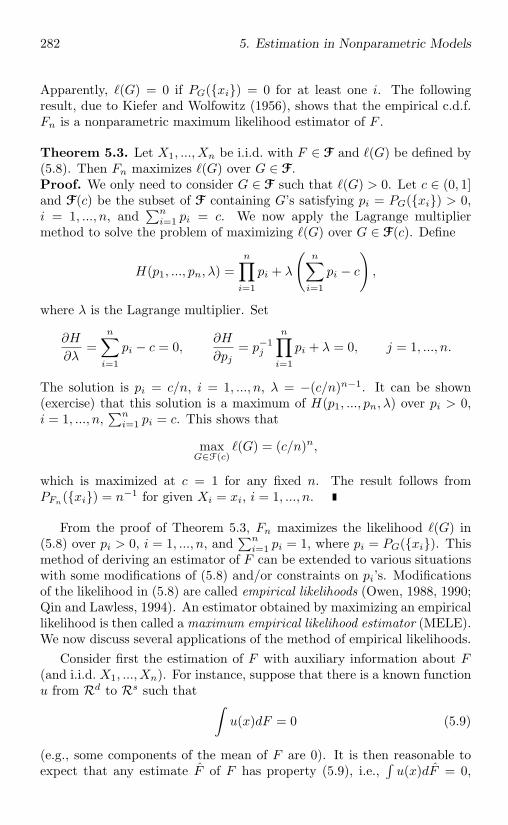
282 5. Estimation in Nonparametric Models
Apparently, (G) = 0 if PG(xi) = 0 for at least one i. The followingresult, due to Kiefer and Wolfowitz (1956), shows that the empirical c.d.f.Fn is a nonparametric maximum likelihood estimator of F .
Theorem 5.3. Let X1, ..., Xn be i.i.d. with F ∈ F and (G) be defined by(5.8). Then Fn maximizes (G) over G ∈ F.Proof. We only need to consider G ∈ F such that (G) > 0. Let c ∈ (0, 1]and F(c) be the subset of F containing G’s satisfying pi = PG(xi) > 0,i = 1, ..., n, and
∑ni=1 pi = c. We now apply the Lagrange multiplier
method to solve the problem of maximizing (G) over G ∈ F(c). Define
H(p1, ..., pn, λ) =n∏
i=1
pi + λ
(n∑
i=1
pi − c
),
where λ is the Lagrange multiplier. Set
∂H
∂λ=
n∑i=1
pi − c = 0,∂H
∂pj= p−1
j
n∏i=1
pi + λ = 0, j = 1, ..., n.
The solution is pi = c/n, i = 1, ..., n, λ = −(c/n)n−1. It can be shown(exercise) that this solution is a maximum of H(p1, ..., pn, λ) over pi > 0,i = 1, ..., n,
∑ni=1 pi = c. This shows that
maxG∈F(c)
(G) = (c/n)n,
which is maximized at c = 1 for any fixed n. The result follows fromPFn(xi) = n−1 for given Xi = xi, i = 1, ..., n.
From the proof of Theorem 5.3, Fn maximizes the likelihood (G) in(5.8) over pi > 0, i = 1, ..., n, and
∑ni=1 pi = 1, where pi = PG(xi). This
method of deriving an estimator of F can be extended to various situationswith some modifications of (5.8) and/or constraints on pi’s. Modificationsof the likelihood in (5.8) are called empirical likelihoods (Owen, 1988, 1990;Qin and Lawless, 1994). An estimator obtained by maximizing an empiricallikelihood is then called a maximum empirical likelihood estimator (MELE).We now discuss several applications of the method of empirical likelihoods.
Consider first the estimation of F with auxiliary information about F(and i.i.d. X1, ..., Xn). For instance, suppose that there is a known functionu from Rd to Rs such that ∫
u(x)dF = 0 (5.9)
(e.g., some components of the mean of F are 0). It is then reasonable toexpect that any estimate F of F has property (5.9), i.e.,
∫u(x)dF = 0,
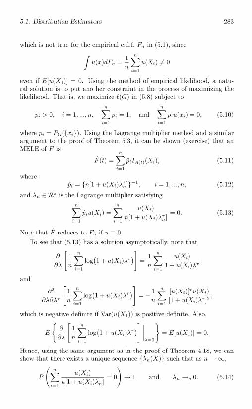
5.1. Distribution Estimators 283
which is not true for the empirical c.d.f. Fn in (5.1), since∫u(x)dFn =
1n
n∑i=1
u(Xi) = 0
even if E[u(X1)] = 0. Using the method of empirical likelihood, a natu-ral solution is to put another constraint in the process of maximizing thelikelihood. That is, we maximize (G) in (5.8) subject to
pi > 0, i = 1, ..., n,n∑
i=1
pi = 1, andn∑
i=1
piu(xi) = 0, (5.10)
where pi = PG(xi). Using the Lagrange multiplier method and a similarargument to the proof of Theorem 5.3, it can be shown (exercise) that anMELE of F is
F (t) =n∑
i=1
piIA(t)(Xi), (5.11)
wherepi = n[1 + u(Xi)λτ
n]−1, i = 1, ..., n, (5.12)
and λn ∈ Rs is the Lagrange multiplier satisfyingn∑
i=1
piu(Xi) =n∑
i=1
u(Xi)n[1 + u(Xi)λτ
n]= 0. (5.13)
Note that F reduces to Fn if u ≡ 0.To see that (5.13) has a solution asymptotically, note that
∂
∂λ
[1n
n∑i=1
log(1 + u(Xi)λτ
)]=
1n
n∑i=1
u(Xi)1 + u(Xi)λτ
and
∂2
∂λ∂λτ
[1n
n∑i=1
log(1 + u(Xi)λτ
)]= − 1
n
n∑i=1
[u(Xi)]τu(Xi)[1 + u(Xi)λτ ]2
,
which is negative definite if Var(u(X1)) is positive definite. Also,
E
∂
∂λ
[1n
n∑i=1
log(1 + u(Xi)λτ
)] ∣∣∣∣λ=0
= E[u(X1)] = 0.
Hence, using the same argument as in the proof of Theorem 4.18, we canshow that there exists a unique sequence λn(X) such that as n → ∞,
P
(n∑
i=1
u(Xi)n[1 + u(Xi)λτ
n]= 0
)→ 1 and λn →p 0. (5.14)
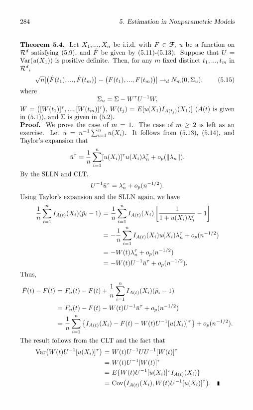
284 5. Estimation in Nonparametric Models
Theorem 5.4. Let X1, ..., Xn be i.i.d. with F ∈ F, u be a function onRd satisfying (5.9), and F be given by (5.11)-(5.13). Suppose that U =Var(u(X1)) is positive definite. Then, for any m fixed distinct t1, ..., tm inRd,
√n[
(F (t1), ..., F (tm)
)−
(F (t1), ..., F (tm)
)] →d Nm(0,Σu), (5.15)
whereΣu = Σ −W τU−1W,
W =([W (t1)]τ , ..., [W (tm)]τ
), W (tj) = E[u(X1)IA(tj)(X1)] (A(t) is given
in (5.1)), and Σ is given in (5.2).Proof. We prove the case of m = 1. The case of m ≥ 2 is left as anexercise. Let u = n−1 ∑n
i=1 u(Xi). It follows from (5.13), (5.14), andTaylor’s expansion that
uτ =1n
n∑i=1
[u(Xi)]τu(Xi)λτn + op(‖λn‖).
By the SLLN and CLT,
U−1uτ = λτn + op(n−1/2).
Using Taylor’s expansion and the SLLN again, we have
1n
n∑i=1
IA(t)(Xi)(pi − 1) =1n
n∑i=1
IA(t)(Xi)[
11 + u(Xi)λτ
n
− 1]
= − 1n
n∑i=1
IA(t)(Xi)u(Xi)λτn + op(n−1/2)
= −W (t)λτn + op(n−1/2)
= −W (t)U−1uτ + op(n−1/2).
Thus,
F (t) − F (t) = Fn(t) − F (t) +1n
n∑i=1
IA(t)(Xi)(pi − 1)
= Fn(t) − F (t) −W (t)U−1uτ + op(n−1/2)
=1n
n∑i=1
IA(t)(Xi) − F (t) −W (t)U−1[u(Xi)]τ
+ op(n−1/2).
The result follows from the CLT and the fact that
Var(W (t)U−1[u(Xi)]τ
)= W (t)U−1UU−1[W (t)]τ
= W (t)U−1[W (t)]τ
= EW (t)U−1[u(Xi)]τIA(t)(Xi)= Cov
(IA(t)(Xi),W (t)U−1[u(Xi)]τ
).
5.1. Distribution Estimators 285
Comparing (5.15) with (5.2), we conclude that F is asymptotically moreefficient than Fn.
Example 5.1 (Survey problems). An example of situations in which wehave auxiliary information expressed as (5.9) is a survey problem (Example2.3) where the population P = y1, ..., yN consists of two-dimensional yj ’s,yj = (y1j , y2j), and the population mean Y2 = N−1 ∑N
j=1 y2j is known.For example, suppose that y1j is the current year’s income of unit j inthe population and y2j is the last year’s income. In many applicationsthe population total or mean of y2j ’s is known, for example, from taxreturn records. Let X1, ..., Xn be a simple random sample (see Example2.3) selected from P with replacement. Then Xi’s are i.i.d. bivariate randomvectors whose c.d.f. is
F (t) =1N
N∑j=1
IA(t)(yj). (5.16)
If Y2 is known, then it can be expressed as (5.9) with u(x1, x2) = x2 − Y2.In survey problems Xi’s are usually sampled without replacement so thatX1, ..., Xn are not i.i.d. However, for a simple random sample withoutreplacement, (5.8) can still be treated as an empirical likelihood, givenXi’s. Note that F in (5.16) is the c.d.f. of Xi, regardless of whether Xi’sare sampled with replacement.
If X = (X1, ..., Xn) is not a simple random sample, then the likelihood(5.8) has to be modified. Suppose that πi is the probability that the ithunit is selected (see Theorem 3.15). Given X = yi, i ∈ s, an empiricallikelihood is
(G) =∏i∈s
[PG(yi)]1/πi =∏i∈s
p1/πi
i , (5.17)
where pi = PG(yi). With the auxiliary information (5.9), an MELE of Fin (5.16) can be obtained by maximizing (G) in (5.17) subject to (5.10).In this case F may not be the c.d.f. of Xi, but the c.d.f.’s of Xi’s aredetermined by F and πi’s. It can be shown (exercise) that an MELE isgiven by (5.11) with
pi =1
πi[1 + u(yi)λτn]
/∑i∈s
1πi
(5.18)
and ∑i∈s
u(yi)πi[1 + u(yi)λτ
n]= 0. (5.19)
If πi = a constant, then the MELE reduces to that in (5.11)-(5.13). If
286 5. Estimation in Nonparametric Models
u(x) = 0 (no auxiliary information), then the MELE is
F (t) =∑i∈s
1πi
IA(t)(yi)/∑
i∈s
1πi
,
which is a ratio of two Horvitz-Thompson estimators (§3.4.2). Some asymp-totic properties of the MELE F can be found in Chen and Qin (1993).
The second part of Example 5.1 shows how to use empirical likelihoodsin a non-i.i.d. problem. Applications of empirical likelihoods in non-i.i.d.problems are usually straightforward extensions of those in i.i.d. cases. Thefollowing is another example.
Example 5.2 (Biased sampling). Biased sampling is often used in applica-tions. Suppose that n = n1 + · · ·+nk, k ≥ 2; Xi’s are independent randomvariables; X1, ..., Xn1 are i.i.d. with F ; and Xnj+1, ..., Xnj+1 are i.i.d. withthe c.d.f. ∫ t
−∞wj+1(s)dF (s)
/∫ ∞
−∞wj+1(s)dF (s),
j = 1, ..., k − 1, where wj ’s are some nonnegative functions. A simpleexample is that X1, ..., Xn1 are sampled from F and Xn1+1, ..., Xn2 aresampled from F but conditional on the fact that each sampled value exceedsa given value x0 (i.e., w2(s) = I(x0,∞)(s)). For instance, Xi’s are bloodpressure measurements; X1, ..., Xn1 are sampled from ordinary people andXn1+1, ..., Xn2 are sampled from patients whose blood pressures are higherthan x0. The name biased sampling comes from the fact that there is abias in the selection of samples.
For simplicity we consider the case of k = 2, since the extension to k ≥ 3is straightforward. Denote w2 by w. An empirical likelihood is
(G) =n1∏i=1
PG(xi)n∏
i=n1+1
w(xi)PG(xi)∫w(s)dG(s)
=
[n∑
i=1
piw(xi)
]−n2 n∏i=1
pi
n∏i=n1+1
w(xi), (5.20)
where pi = PG(xi). An MELE of F can be obtained by maximizing theempirical likelihood (5.20) subject to pi > 0, i = 1, ..., n, and
∑ni=1 pi =
1. Using the Lagrange multiplier method we can show (exercise) that anMELE F is given by (5.11) with
pi = [n1 + n2w(Xi)/w]−1, i = 1, ..., n, (5.21)
5.1. Distribution Estimators 287
where w satisfies
w =n∑
i=1
w(Xi)n1 + n2w(Xi)/w
.
An asymptotic result similar to that in Theorem 5.4 can be established(Vardi, 1985; Qin, 1993).
Our last example concerns an important application in survival analysis.
Example 5.3 (Censored data). Let Z1, ..., Zn be survival times that arei.i.d. nonnegative random variables from a c.d.f. F , and Y1, ..., Yn be i.i.d.nonnegative random variables independent of Zi’s. In a variety of applica-tions in biostatistics and life-time testing, we are only able to observe thesmaller of Zi and Yi and an indicator of which variables is smaller:
Xi = min(Zi, Yi), δi = I(0,Yi)(Zi), i = 1, ..., n.
This is called a random censorship model and Yi’s are called censoring times.We consider the estimation of the survival distribution F ; see Kalbfleischand Prentice (1980) for other problems involving censored data.
An MELE of F can be derived as follows. Let x(1) ≤ · · · ≤ x(n) beordered values of Xi’s and δ(i) be the δ-value associated with x(i). Considera c.d.f. G that assigns its mass to the points x(1), ..., x(n) and the interval(x(n),∞). Let pi = PG(x(i)), i = 1, ..., n, and pn+1 = 1 − G(x(n)). AnMELE of F is then obtained by maximizing
(G) =n∏
i=1
pδ(i)i
⎛⎝ n+1∑j=i+1
pj
⎞⎠1−δ(i)
(5.22)
subject to
pi > 0, i = 1, ..., n + 1,n+1∑i=1
pi = 1. (5.23)
It can be shown (exercise) that an MELE is
F (t) =n+1∑i=1
piI(X(i−1),X(i))(t), (5.24)
where X(0) = 0, X(n+1) = ∞, X(1) ≤ · · · ≤ X(n) are order statistics, and
p1 = 1n , pi = δ(i)
n−i+1
i−1∏j=1
(1 − δ(j)
n−j+1
), i = 2, ..., n, pn+1 = 1 −
n∑j=1
pj .
288 5. Estimation in Nonparametric Models
The F in (5.24) can also be written as (exercise)
F (t) = 1 −∏
X(i)≤t
(1 − δ(i)
n−i+1
), (5.25)
which is the well-known Kaplan-Meier (1958) product-limit estimator. Someasymptotic results for F in (5.25) can be found, for example, in Shorackand Wellner (1986).
5.1.3 Density estimation
Suppose that X1, ..., Xn are i.i.d. random variables from F and that F isunknown but has a Lebesgue p.d.f. f . Estimation of F can be done byestimating f , which is called density estimation. Note that estimators of Fderived in §5.1.1 and §5.1.2 do not have Lebesgue p.d.f.’s.
Since f(t) = F ′(t) a.e., a simple estimator of f(t) is the differencequotient
fn(t) =Fn(t + λn) − Fn(t− λn)
2λn, t ∈ R, (5.26)
where Fn is the empirical c.d.f. given by (2.31) or (5.1) with d = 1, andλn is a sequence of positive constants. Since 2nλnfn(t) has the binomialdistribution Bi(F (t + λn) − F (t− λn), n),
E[fn(t)] → f(t) if λn → 0 as n → ∞
andVar
(fn(t)
)→ 0 if λn → 0 and nλn → ∞.
Thus, we should choose λn converging to 0 slower than n−1. If we assumethat λn → 0, nλn → ∞, and f is continuously differentiable at t, then itcan be shown (exercise) that
msefn(t)(F ) =f(t)2nλn
+ o
(1
nλn
)+ O(λ2
n) (5.27)
and, under the additional condition that nλ3n → 0,√
nλn[fn(t) − f(t)] →d N(0, 1
2f(t)). (5.28)
A useful class of estimators is the class of kernel density estimators ofthe form
f(t) =1
nλn
n∑i=1
w(
t−Xi
λn
), (5.29)
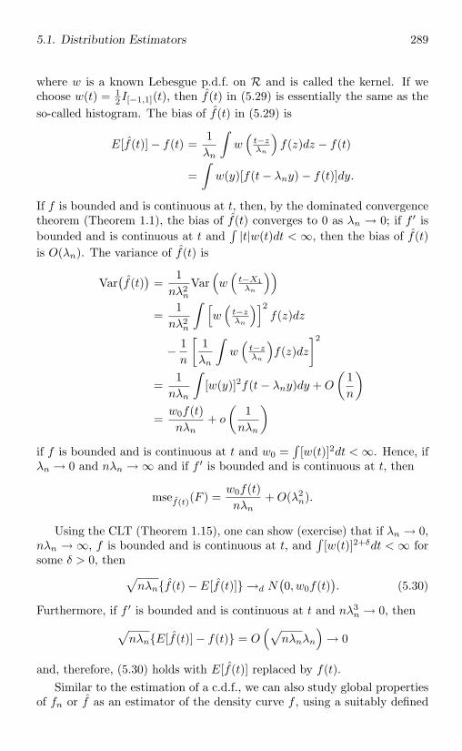
5.1. Distribution Estimators 289
where w is a known Lebesgue p.d.f. on R and is called the kernel. If wechoose w(t) = 1
2I[−1,1](t), then f(t) in (5.29) is essentially the same as theso-called histogram. The bias of f(t) in (5.29) is
E[f(t)] − f(t) =1λn
∫w
(t−zλn
)f(z)dz − f(t)
=∫
w(y)[f(t− λny) − f(t)]dy.
If f is bounded and is continuous at t, then, by the dominated convergencetheorem (Theorem 1.1), the bias of f(t) converges to 0 as λn → 0; if f ′ isbounded and is continuous at t and
∫|t|w(t)dt < ∞, then the bias of f(t)
is O(λn). The variance of f(t) is
Var(f(t)
)=
1nλ2
n
Var(w
(t−X1λn
))=
1nλ2
n
∫ [w
(t−zλn
)]2f(z)dz
− 1n
[1λn
∫w
(t−zλn
)f(z)dz
]2
=1
nλn
∫[w(y)]2f(t− λny)dy + O
(1n
)=
w0f(t)nλn
+ o
(1
nλn
)if f is bounded and is continuous at t and w0 =
∫[w(t)]2dt < ∞. Hence, if
λn → 0 and nλn → ∞ and if f ′ is bounded and is continuous at t, then
msef(t)(F ) =w0f(t)nλn
+ O(λ2n).
Using the CLT (Theorem 1.15), one can show (exercise) that if λn → 0,nλn → ∞, f is bounded and is continuous at t, and
∫[w(t)]2+δdt < ∞ for
some δ > 0, then√nλnf(t) − E[f(t)] →d N
(0, w0f(t)
). (5.30)
Furthermore, if f ′ is bounded and is continuous at t and nλ3n → 0, then√
nλnE[f(t)] − f(t) = O(√
nλnλn
)→ 0
and, therefore, (5.30) holds with E[f(t)] replaced by f(t).Similar to the estimation of a c.d.f., we can also study global properties
of fn or f as an estimator of the density curve f , using a suitably defined
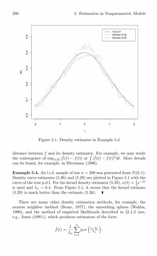
290 5. Estimation in Nonparametric Models
t
f(t)
-2 -1 0 1 2
0.0
0.1
0.2
0.3
0.4
0.5
True p.d.fEstimator (5.26)Estimator (5.29)
Figure 5.1: Density estimates in Example 5.4
distance between f and its density estimator. For example, we may studythe convergence of supt∈R |f(t) − f(t)| or
∫|f(t) − f(t)|2dt. More details
can be found, for example, in Silverman (1986).
Example 5.4. An i.i.d. sample of size n = 200 was generated from N(0, 1).Density curve estimates (5.26) and (5.29) are plotted in Figure 5.1 with thecurve of the true p.d.f. For the kernel density estimator (5.29), w(t) = 1
2e−|t|
is used and λn = 0.4. From Figure 5.1, it seems that the kernel estimate(5.29) is much better than the estimate (5.26).
There are many other density estimation methods, for example, thenearest neighbor method (Stone, 1977), the smoothing splines (Wahba,1990), and the method of empirical likelihoods described in §5.1.2 (see,e.g., Jones (1991)), which produces estimators of the form
f(t) =1λn
n∑i=1
piw(
t−Xi
λn
).
5.2. Statistical Functionals 291
5.2 Statistical Functionals
In many nonparametric problems we are interested in estimating some char-acteristics (parameters) of the unknown population, not the entire popula-tion. We assume in this section that Xi’s are i.i.d. from an unknown c.d.f.F on Rd. Most characteristics of F can be written as T(F ), where T is afunctional from F to Rs. If we estimate F by the empirical c.d.f. Fn in(5.1), then a natural estimator of T(F ) is T(Fn), which is called a statisticalfunctional.
Many commonly used statistics can be written as T(Fn) for some T.Two simple examples are given as follows. Let T(F ) =
∫ψ(x)dF (x) with an
integrable function ψ, and T(Fn) =∫ψ(x)dFn(x) = n−1 ∑n
i=1 ψ(Xi). Thesample moments discussed in §3.5.2 are particular examples of this kind ofstatistical functionals. For d = 1, let T(F ) = F−1(p) = infx : F (x) ≥ p,where p ∈ (0, 1) is a fixed constant. F−1(p) is called the pth quantile of F .The statistical functional T(Fn) = F−1
n (p) is called the pth sample quantile.More examples of statistical functionals are provided in §5.2.1 and §5.2.2.
In this section we study asymptotic distributions of T(Fn). We focus onthe case of real-valued T (s = 1), since the extension to the case of s ≥ 2 isstraightforward.
5.2.1 Differentiability and asymptotic normality
Note that T(Fn) is a function of the “statistic” Fn. In Theorem 1.12 (and§3.5.1) we have studied how to use Taylor’s expansion to establish asymp-totic normality of differentiable functions of statistics that are asymptot-ically normal. This leads to the approach of establishing asymptotic nor-mality of T(Fn) by using some generalized Taylor expansions for functionalsand using asymptotic properties of Fn given in §5.1.1.
First, we need a suitably defined differential of T. Several versions ofdifferentials are given in the following definition.
Definition 5.2. Let T be a functional on F0, a collection of c.d.f.’s on Rd,and let D = c(G1 −G2) : c ∈ R, Gj ∈ F0, j = 1, 2.(i) A functional T on F0 is Gateaux differentiable at G ∈ F0 if and only ifthere is a linear functional LG on D (i.e., LG(c1∆1 + c2∆2) = c1LG(∆1) +c2LG(∆2) for any ∆j ∈ D and cj ∈ R) such that ∆ ∈ D and G + t∆ ∈ F0imply
limt→0
[T(G + t∆) − T(G)
t− LG(∆)
]= 0.
(ii) Let be a distance on F0. Suppose that ‖c(G1 −G2)‖ = |c|(G1, G2),c ∈ R, Gj ∈ F0, defines a norm on D (i.e., ‖∆‖ ≥ 0 and = 0 if and only
292 5. Estimation in Nonparametric Models
if ∆ = 0, ‖c∆‖ = |c|‖∆‖, and ‖∆ + ∆‖ ≤ ‖∆‖ + ‖∆‖, ∆ ∈ D, ∆ ∈ D,c ∈ R). A functional T on F0 is -Hadamard differentiable at G ∈ F0 ifand only if there is a linear functional LG on D such that for any sequenceof numbers tj → 0 and ∆,∆j , j = 1, 2, ... ⊂ D satisfying ‖∆j − ∆‖ → 0and G + tj∆j ∈ F0,
limj→∞
[T(G + tj∆j) − T(G)
tj− LG(∆j)
]= 0.
(iii) Let be a distance on F0. A functional T on F0 is -Frechet differen-tiable at G ∈ F0 if and only if there is a linear functional LG on D suchthat for any sequence Gj satisfying Gj ∈ F0 and (Gj , G) → 0,
limj→∞
T(Gj) − T(G) − LG(Gj −G)(Gj , G)
= 0.
The functional LG is called the differential of T at G. If we defineh(t) = T(G + t∆), then the Gateaux differentiability is equivalent to thedifferentiability of the function h(t) at t = 0, and LG(∆) is simply h′(0). Letδx denote the d-dimensional c.d.f. degenerated at the point x and φG(x) =LG(δx − G). Then φF (x) is called the influence function of T at F , whichis an important tool in robust statistics (see Hampel (1974)).
If T is Gateaux differentiable at F , then we have the following expansion(taking t = n−1/2 and ∆ =
√n(Fn − F )):
√n[T(Fn) − T(F )] = LF
(√n(Fn − F )
)+ Rn. (5.31)
Since LF is linear,
LF(√
n(Fn − F ))
=1√n
n∑i=1
φF (Xi) →d N(0, σ2F ) (5.32)
by the CLT, provided that
E[φF (X1)] = 0 and σ2F = E[φF (X1)]2 < ∞ (5.33)
(which is usually true when φF is bounded or when F has some finitemoments). By Slutsky’s theorem and (5.32),
√n[T(Fn) − T(F )] →d N(0, σ2
F ) (5.34)
if Rn in (5.31) is op(1).Unfortunately, Gateaux differentiability is too weak to be useful in es-
tablishing Rn = op(1) (or (5.34)). This is why we need other types of
5.2. Statistical Functionals 293
differentiability. Hadamard differentiability, which is also referred to ascompact differentiability, is clearly stronger than Gateaux differentiabilitybut weaker than Frechet differentiability (exercise). For a given functionalT, we can first find LG by differentiating h(t) = T(G+ t∆) at t = 0 and thencheck whether T is -Hadamard (or -Frechet) differentiable with a given .The most commonly used distances on F0 are the sup-norm distance ∞in (5.3) and the Lp distance Lp
in (5.5). Their corresponding norms on D
are ‖∆‖∞=supx |∆(x)| and ‖∆‖Lp =[∫|∆(x)|pdx]1/p, ∆ ∈ D.
Theorem 5.5. Let X1, ..., Xn be i.i.d. from a c.d.f. F on Rd.(i) If T is ∞-Hadamard differentiable at F , then Rn in (5.31) is op(1).(ii) If T is -Frechet differentiable at F with a distance satisfying
√n(Fn, F ) = Op(1), (5.35)
then Rn in (5.31) is op(1).(iii) In either (i) or (ii), if (5.33) is also satisfied, then (5.34) holds.Proof. Part (iii) follows directly from (i) or (ii). The proof of (i) involvessome high-level mathematics and is omitted; see, for example, Fernholz(1983). We now prove (ii). From Definition 5.2(iii), for any ε > 0, there isa δ > 0 such that |Rn| < ε
√n(Fn, F ) whenever (Fn, F ) < δ. Then
P (|Rn| > η) ≤ P(√
n(Fn, F ) > η/ε)
+ P ((Fn, F ) ≥ δ)
for any η > 0, which implies
lim supn
P (|Rn| > η) ≤ lim supn
P(√
n(Fn, F ) > η/ε).
The result follows from (5.35) and the fact that ε can be arbitrarily small.
Since -Frechet differentiability implies -Hadamard differentiability,Theorem 5.5(ii) is useful when is not the sup-norm distance. Thereare functionals that are not ∞-Hadamard differentiable (and hence not∞-Frechet differentiable). For example, if d = 1 and T(G) = g(
∫xdG)
with a differentiable function g, then T is not necessarily ∞-Hadamarddifferentiable, but is L1
-Frechet differentiable (exercise).From Theorem 5.2, condition (5.35) holds for Lp
under the momentconditions on F given in Theorem 5.2.
Note that if and are two distances on F0 satisfying (G1, G2) ≤c(G1, G2) for a constant c and all Gj ∈ F0, then -Hadamard (Frechet)differentiability implies -Hadamard (Frechet) differentiability. This sug-gests the use of the distance ∞+p = ∞ + Lp
, which also satisfies (5.35)under the moment conditions in Theorem 5.2. The distance ∞+p is usefulin some cases (Theorem 5.6).
294 5. Estimation in Nonparametric Models
A ∞-Hadamard differentiable T having a bounded and continuous in-fluence function φF is robust in Hampel’s sense (see, e.g., Huber (1981)).This is motivated by the fact that the asymptotic behavior of T(Fn) is de-termined by that of LF (Fn − F ), and a small change in the sample, i.e.,small changes in all xi’s (rounding, grouping) or large changes in a few ofxi’s (gross errors, blunders), will result in a small change of T(Fn) if andonly if φF is bounded and continuous.
We now consider some examples. For the sample moments related tofunctionals of the form T(G) =
∫ψ(x)dG(x), it is clear that T is a linear
functional. Any linear functional is trivially -Frechet differentiable for any. Next, if F is one-dimensional and F ′(x) > 0 for all x, then the quantilefunctional T(G) = G−1(p) is ∞-Hadamard differentiable at F (Fernholz,1983). Hence, Theorem 5.5 applies to these functionals. But the asymptoticnormality of sample quantiles can be established under weaker conditions,which are studied in §5.3.1.
Example 5.5 (Convolution functionals). Suppose that F is on R and fora fixed z ∈ R,
T(G) =∫
G(z − y)dG(y), G ∈ F.
If X1 and X2 are i.i.d. with c.d.f. G, then T(G) is the c.d.f. of X1 + X2(Exercise 42 in §1.6), and is also called the convolution of G evaluated atz. For tj → 0 and ‖∆j − ∆‖∞ → 0,
T(G + tj∆j) − T(G) = 2tj∫
∆j(z − y)dG(y) + t2j
∫∆j(z − y)d∆j(y)
(for ∆ = c1G1 + c2G2, Gj ∈ F0, and cj ∈ R, d∆ denotes c1dG1 + c2dG2).Using Lemma 5.2, one can show (exercise) that∫
∆j(z − y)d∆j(y) = O(1). (5.36)
Hence T is ∞-Hadamard differentiable at any G ∈ F with LG(∆) =2∫
∆(z−y)dG(y). The influence function, φF (x) = 2∫
(δx−F )(z−y)dF (y),is a bounded function and clearly satisfies (5.33). Thus, (5.34) holds. If Fis continuous, then T is robust in Hampel’s sense (exercise).
Three important classes of statistical functionals, i.e., L-estimators, M-estimators, and rank statistics and R-estimators, are considered in §5.2.2.
Lemma 5.2. Let ∆ ∈ D and h be a function on R such that∫h(x)d∆(x)
is finite. Then ∣∣∣∣ ∫ h(x)d∆(x)∣∣∣∣ ≤ ‖h‖V ‖∆‖∞,
5.2. Statistical Functionals 295
where ‖h‖V is the variation norm defined by
‖h‖V = lima→−∞,b→∞
⎡⎣supm∑j=1
|h(xj) − h(xj−1)|
⎤⎦with the supremum being taken over all partitions a = x0 < · · · < xm = bof the interval [a, b].
The proof of Lemma 5.2 can be found, for example, in Natanson (1961,p. 232).
The differentials in Definition 5.2 are first-order differentials. For somefunctionals, we can also consider their second-order differentials.
Definition 5.3. Let T be a functional on F0 and be a distance on F0.(i) T is second-order -Hadamard differentiable at G ∈ F0 if and only ifthere is a functional QG on D such that for any sequence of numbers tj → 0and ∆,∆j , j = 1, 2, ... ⊂ D satisfying ‖∆j −∆‖ → 0 and G+ tj∆j ∈ F0,
limj→∞
T(G + tj∆j) − T(G) − QG(tj∆j)t2j
= 0,
where QG(∆) =∫ ∫
ψG(x, y)d(G+ tj∆)(x)d(G+ tj∆)(y) for a function ψG
satisfying ψG(x, y) = ψG(y, x),∫ ∫
ψG(x, y)dG(x)dG(y) = 0, and ‖ · ‖ isthe same as that in Definition 5.2(ii).(ii) T is second-order -Frechet differentiable at G ∈ F0 if and only if, forany sequence Gj satisfying Gj ∈ F0 and (Gj , G) → 0,
limj→∞
T (Gj) − T (G) − QG(Gj −G)[(Gj , G)]2
= 0,
where QG is the same as that in (i).
For a second-order differentiable T, we have the following expansion:
n[T(Fn) − T(F )] = nVn + Rn, (5.37)
where
Vn = QG(Fn − F ) =∫ ∫
ψF (x, y)dFn(x)dFn(y) =1n2
n∑j=1
n∑i=1
ψF (Xi, Xj)
is a “V-statistic” (§3.5.3) whose asymptotic properties are given by The-orem 3.16. If Rn in (5.37) is op(1), then the asymptotic behavior ofT(Fn) − T(F ) is the same as that of Vn.
296 5. Estimation in Nonparametric Models
Proposition 5.1. Let X1, ..., Xn be i.i.d. from F .(i) If T is second-order ∞-Hadamard differentiable at F , then Rn in (5.37)is op(1).(ii) If T is second-order -Frechet differentiable at F with a distance satisfying (5.35), then Rn in (5.37) is op(1).
Combining Proposition 5.1 with Theorem 3.16, we can summarize theasymptotic behavior of T(Fn) − T(F ) as follows. If
ζ1 = Var(∫
ψF (X1, y)dF (y))
is positive, then (5.34) holds with σ2F = 4ζ1. If ζ1 = 0, then
n[T(Fn) − T(F )] →d
∞∑j=1
λjχ21j .
If T is also first-order differentiable, then it can be shown (exercise) that
φF (x) = 2∫
ψF (x, y)dF (y). (5.38)
Then ζ1 = 4−1Var(φF (X1)) and ζ1 = 0 corresponds to the case of φF (x) ≡0. However, second-order -Hadamard (Frechet) differentiability does notin general imply first-order -Hadamard (Frechet) differentiability (exer-cise).
The technique in this section can be applied to non-i.i.d. Xi’s when thec.d.f.’s of Xi’s are determined by an unknown c.d.f. F , provided that resultssimilar to (5.32) and (5.35) (with Fn replaced by some other estimator F )can be established.
5.2.2 L-, M-, R-estimators and rank statistics
Three large classes of statistical functionals based on i.i.d. Xi’s are studiedin this section.
L-estimators
Let F be a c.d.f. on R and J(t) be a function on [0, 1]. An L-functional isdefined as
T(G) =∫
xJ(G(x))dG(x), G ∈ F. (5.39)
T(Fn) is called an L-estimator of T(F ).
5.2. Statistical Functionals 297
Example 5.6. The following are some examples of commonly used L-estimators.(i) When J ≡ 1, T(Fn) = X, the sample mean.(ii) When J(t) = 4t− 2, T(Fn) is called Gini’s mean difference.(iii) When J(t) = (β − α)−1I(α,β)(t) for some constants α < β, T(Fn) iscalled the trimmed sample mean.
For an L-functional T, it can be shown (exercise) that
T(G) − T(F ) =∫
φF (x)d(G− F )(x) + R(G,F ), (5.40)
whereφF (x) = −
∫(δx − F )(y)J(F (y))dy, (5.41)
R(G,F ) = −∫
WG(x)[G(x) − F (x)]dx,
and
WG(x) =
[G(x) − F (x)]−1
∫ G(x)F (x) J(t)dt− J(F (x)) G(x) = F (x)
0 G(x) = F (x).
A sufficient condition for (5.33) in this case is that F has a finite vari-ance (exercise). However, (5.33) is also satisfied if φF is bounded. Thedifferentiability of T can be verified under some conditions on J .
Theorem 5.6. Let T be an L-functional defined by (5.39).(i) Suppose that J is bounded, J(t) = 0 when t ∈ [0, α] ∪ [β, 1] for someconstants α < β, and that the set D = x : J is discontinuous at F (x)has Lebesgue measure 0. Then T is ∞-Frechet differentiable at F with theinfluence function φF given by (5.41), and φF is bounded and continuousand satisfies (5.33).(ii) Suppose that J is bounded, the set D in (i) has Lebesgue measure 0,and J is continuous on [0, α] ∪ [β, 1] for some constants α < β. Then T is∞+1-Frechet differentiable at F .(iii) Suppose that |J(t) − J(s)| ≤ C|t − s|p−1, where C > 0 and p > 1 aresome constants. Then T is Lp
-Frechet differentiable at F .(iv) If, in addition to the conditions in part (i), J ′ is continuous on [α, β],then T is second-order ∞-Frechet differentiable at F with
ψF (x, y) = φF (x) + φF (y) −∫
(δx − F )(z)(δy − F )(z)J ′(F (z))dz.
(v) Suppose that J ′ is continuous on [0, 1]. Then T is second-order L2-
Frechet differentiable at F with the same ψF given in (iv).
298 5. Estimation in Nonparametric Models
Proof. We prove (i)-(iii). The proofs for (iv) and (v) are similar and areleft to the reader.(i) Let Gj ∈ F and ∞(Gj , F ) → 0. Let c and d be two constants such thatF (c) > β and F (d) < α. Then, for sufficiently large j, Gj(x) ∈ [0, α]∪ [β, 1]if x > c or x < d. Hence, for sufficiently large j,
|R(Gj , F )| =∣∣∣∣ ∫ c
d
WGj(x)(Gj − F )(x)dx
∣∣∣∣≤ ∞(Gj , F )
∫ c
d
|WGj(x)|dx.
Since J is continuous at F (x) when x ∈ D and D has Lebesgue measure0, WGj (x) → 0 a.e. Lebesgue. By the dominated convergence theorem,∫ c
d|WGj
(x)|dx → 0. This proves that T is ∞-Frechet differentiable. Theassertions on φF can be proved by noting that
φF (x) = −∫ c
d
(δx − F )(y)J(F (y))dy.
(ii) From the proof of (i), we only need to show that∣∣∣∣ ∫A
WGj(x)(Gj − F )(x)dx
∣∣∣∣/∞+1(Gj , F ) → 0, (5.42)
where A = x : F (x) ≤ α or F (x) > β. The quantity on the left-handside of (5.42) is bounded by supx∈A |WGj
(x)| which converges to 0 underthe continuity assumption of J on [0, α] ∪ [β, 1]. Hence (5.42) follows.(iii) The result follows from
|R(G,F )| ≤ C
∫|G(x) − F (x)|pdx = O
([Lp
(G,F )]p)
and the fact that p > 1.
An L-estimator with J(t) = 0 when t ∈ [0, α]∪ [β, 1] is called a trimmedL-estimator. Theorem 5.6(i) shows that trimmed L-estimators satisfy (5.34)and are robust in Hampel’s sense. In case (ii) or (iii) of Theorem 5.6, (5.34)holds if Var(X1) < ∞, but T(Fn) may not be robust in Hampel’s sense. Itcan be shown (exercise) that one or several of (i)-(v) of Theorem 5.6 canbe applied to each of the L-estimators in Example 5.6.
M-estimators
Let F be a c.d.f. on Rd and ρ(x, t) be a Borel function on Rd × R. AnM-functional is defined to be a solution of∫
ρ(x, T(G))dG(x) = mint∈Θ
∫ρ(x, t)dG(x), G ∈ F, (5.43)
5.2. Statistical Functionals 299
where Θ is an open subset of R. T(Fn) is called an M-estimator of T(F ).Assume that ψ(x, t) = ∂ρ(x, t)/∂t exists a.e. and
λG(t) =∫
ψ(x, t)dG(x) =∂
∂t
∫ρ(x, t)dG(x). (5.44)
Then λG(T(G)) = 0.
Example 5.7. The following are some examples of M-estimators.(i) If ρ(x, t) = (x − t)2/2, then ψ(x, t) = t − x; T(G) =
∫xdG(x) is the
mean functional; and T(Fn) = X is the sample mean.(ii) If ρ(x, t) = |x− t|p/p, where p ∈ [1, 2), then
ψ(x, t) =
⎧⎨⎩|x− t|p−1 x < t
0 x = t
−|x− t|p−1 x > t.
If p = 1, T(Fn) is the sample median. If 1 < p < 2, T (Fn) is called the pthleast absolute deviations estimator or the minimum Lp distance estimator.(iii) Let F0 = fθ : θ ∈ Θ be a parametric family of p.d.f.’s and ρ(x, t) =− log ft(x). Then T(Fn) is an MLE. This indicates that M-estimators areextensions of MLE’s in parametric models.(iv) Huber (1964) considers
ρ(x, t) = 1
2 (x− t)2 |x− t| ≤ C
C2 |x− t| > C
with
ψ(x, t) =
t− x |x− t| ≤ C
0 |x− t| > C.
The corresponding T(Fn) is a type of trimmed sample mean.(v) Huber (1964) considers
ρ(x, t) = 1
2 (x− t)2 |x− t| ≤ C
C|x− t| − 12C
2 |x− t| > C
with
ψ(x, t) =
⎧⎨⎩C t− x > C
t− x |x− t| ≤ C
−C t− x < −C.
The corresponding T(Fn) is a type of Winsorized sample mean.(vi) Hampel (1974) considers ψ(x, t) = ψ0(t − x) with ψ0(s) = −ψ0(−s)and
ψ0(s) =
⎧⎪⎪⎪⎨⎪⎪⎪⎩s 0 ≤ s ≤ a
a a < s ≤ ba(c−s)c−b b < s ≤ c
0 s > c,
300 5. Estimation in Nonparametric Models
where 0 < a < b < c are constants. A smoothed version of ψ0 is
ψ1(s) =
sin(as) 0 ≤ s < π/a
0 s > π/a.
For bounded and continuous ψ, the following result shows that T is ∞-Hadamard differentiable with a bounded and continuous influence functionand, hence, T(Fn) satisfies (5.34) and is robust in Hampel’s sense.
Theorem 5.7. Let T be an M-functional defined by (5.43). Assume thatψ is a bounded and continuous function on Rd × R and that λF (t) iscontinuously differentiable at T(F ) and λ′
F (T(F )) = 0. Then T is ∞-Hadamard differentiable at F with
φF (x) = −ψ(x, T(F ))/λ′F (T(F )).
Proof. Let tj → 0, ∆j ∈ D, ‖∆j − ∆‖∞ → 0, and Gj = F + tj∆j ∈ F.Since λG(T(G)) = 0,
|λF (T(Gj)) − λF (T(F ))| =∣∣∣∣tj ∫ ψ(x, T(Gj))d∆j(x)
∣∣∣∣ → 0
by ‖∆j − ∆‖∞ → 0 and the boundedness of ψ. Note that λ′F (T(F )) = 0.
Hence, the inverse of λF (t) exists and is continuous in a neighborhood of0 = λF (T(F )). Therefore,
T(Gj) − T(F ) → 0. (5.45)
Let hF (T(F )) = λ′F (T(F )), hF (t) = [λF (t) − λF (T(F ))]/[t − T(F )] if t =
T(F ),
R1j =∫
ψ(x, T(F ))d∆j(x)[
1λ′F (T(F ))
− 1hF (T(Gj))
],
R2j =1
hF (T(Gj))
∫[ψ(x, T(Gj)) − ψ(x, T(F ))]d∆j(x),
andLF (∆) = − 1
λ′F (T(F ))
∫ψ(x, T(F ))d∆(x), ∆ ∈ D.
ThenT(Gj) − T(F ) = −LF (tj∆j) + tj(R1j −R2j).
By (5.45), ‖∆j − ∆‖∞ → 0, and the boundedness of ψ, Rj1 → 0. Theresult then follows from R2j → 0, which follows from ‖∆j −∆‖∞ → 0 andthe boundedness and continuity of ψ (exercise).
5.2. Statistical Functionals 301
Some ψ functions in Example 5.7 satisfy the conditions in Theorem5.7 (exercise). Under more conditions on ψ, it can be shown that an M-functional is ∞-Frechet differentiable at F (Clarke, 1986; Shao, 1993).Some M-estimators that satisfy (5.34) but are not differentiable functionalsare studied in §5.4.
Rank statistics and R-estimators
Assume that X1, ..., Xn are i.i.d. from a c.d.f. F on R. The rank of Xi
among X1, ..., Xn, denoted by Ri, is defined to be the number of Xj ’ssatisfying Xj ≤ Xi, i = 1, ..., n. The rank of |Xi| among |X1|, ..., |Xn| issimilarly defined and denoted by Ri. A statistic that is a function of Ri’sor Ri’s is called a rank statistic. For G ∈ F, let
G(x) = G(x) −G((−x)−
), x > 0,
where g(x−) denotes the left limit of the function g at x. Define a functionalT by
T(G) =∫ ∞
0J(G(x))dG(x), G ∈ F, (5.46)
where J is a function on [0, 1] with a bounded J ′. Then
T(Fn) =∫ ∞
0J(Fn(x))dFn(x) =
1n
n∑i=1
J(
Ri
n
)I(0,∞)(Xi)
is a (one-sample) signed rank statistic. If J(t) = t, then T(Fn) is the well-known Wilcoxon signed rank test (§6.5.1).
Statistics based on ranks (or signed ranks) are robust against changes invalues of xi’s, but may not provide efficient inference procedures, since thevalues of xi’s are discarded after ranks (or signed ranks) are determined.
It can be shown (exercise) that T in (5.46) is ∞-Hadamard differentiableat F with the differential
LF (∆) =∫ ∞
0J ′(F (x))∆(x)dF (x) +
∫ ∞
0J(F (x))d∆(x). (5.47)
These results can be extended to the case where X1, ..., Xn are i.i.d.from a c.d.f. F on R2. For any c.d.f. G on R2, let J be a function on [0, 1]with J(1 − t) = −J(t) and a bounded J ′,
G(y) = [G(y,∞) + G(∞, y)]/2, y ∈ R,
andT(G) =
∫J(G(y))dG(y,∞). (5.48)
302 5. Estimation in Nonparametric Models
Let Xi = (Yi, Zi), Ri be the rank of Yi, and Ui be the number of Zj ’ssatisfying Zj ≤ Yi, i = 1, ..., n. Then
T(Fn) =∫
J(Fn(y))dFn(y,∞) =1n
n∑i=1
J(Ri+Ui
2n
)is called a two-sample linear rank statistic. It can be shown (exercise) thatT in (5.48) is ∞-Hadamard differentiable at F with the differential
LF (∆) =∫
J ′(F (y))∆(y)dF (y,∞) +∫
J(F (y))d∆(y,∞). (5.49)
Rank statistics (one-sample or two-sample) are asymptotically normaland robust in Hampel’s sense (exercise). These results are useful in testinghypotheses (§6.5).
Let F be a continuous c.d.f. on R symmetric about an unknown pa-rameter θ ∈ R. An estimator of θ closely related to a rank statistic can bederived as follows. Let Xi be i.i.d. from F and Wi = (Xi, 2t −Xi) with afixed t ∈ R. The functional T in (5.48) evaluated at the c.d.f. of Wi is equalto
λF (t) =∫
J(
F (x)+1−F (2t−x)2
)dF (x). (5.50)
If J is strictly increasing and F is strictly increasing in a neighborhood ofθ, then λF (t) = 0 if and only if t = θ (exercise). For G ∈ F, define T(G) tobe a solution of ∫
J(
G(x)+1−G(2T(G)−x)2
)dG(x) = 0. (5.51)
T(Fn) is called an R-estimator of T(F ) = θ. When J(t) = t − 12 (which is
related to the Wilcoxon signed rank test), T(Fn) is the well-known Hodges-Lehmann estimator and is equal to any value between the two middle pointsof the values (Xi + Xj)/2, i = 1, ..., n, j = 1, ..., n.
Theorem 5.8. Let T be the functional defined by (5.51). Suppose thatF is continuous and symmetric about θ, the derivatives F ′ and J ′ exist,and J ′ is bounded. Then T is ∞-Hadamard differentiable at F with theinfluence function
φF (x) =J(F (x))∫
J ′(F (x))F ′(x)dF (x).
Proof. Since F is symmetric about θ, F (x) + F (2θ − x) = 1. Underthe assumed conditions, λF (t) is continuous and
∫J ′(F (x))F ′(x)dF (x) =
−λ′F (θ) = 0 (exercise). Hence the inverse of λF exists and is continuous
5.2. Statistical Functionals 303
at 0 = λF (θ). Suppose that tj → 0, ∆j ∈ D, ‖∆j − ∆‖∞ → 0, andGj = F + tj∆j ∈ F. Then∫
[J(Gj(x, t)) − J(F (x, t))]dGj(x) → 0
uniformly in t, where G(x, t) = [G(x) + 1 −G(2t− x)]/2, and∫J(F (x, t))d(Gj − F )(x) =
∫(Gj − F )(x)J ′(F (x, t))dF (x, t) → 0
uniformly in t. Let λG(t) be defined by (5.50) with F replaced by G. Then
λGj(t) − λF (t) → 0
uniformly in t. Thus, λF (T(Gj)) → 0, which implies
T(Gj) → T(F ) = θ. (5.52)
Let ξG(t) =∫J(F (x, t))dG(x), hF (t) = [λF (t) − λF (θ)]/(t − θ) if t = θ,
and hF (θ) = λ′F (θ). Then T(Gj)− T(F )−
∫φF (x)d(Gj −F )(x) is equal to
ξGj (θ)[
1λ′F (θ)
− 1hF (T(Gj))
]+
λF (T(Gj)) − ξGj (θ)hF (T(Gj))
. (5.53)
Note that
ξGj (θ) =∫
J(F (x))dGj(x) = tj
∫J(F (x))d∆j(x).
By (5.52), Lemma 5.2, and ‖∆j−∆‖∞ → 0, the first term in (5.53) is o(tj).The second term in (5.53) is the sum of
− tjhF (T(Gj))
∫[J(F (x, T(Gj))) − J(F (x))]d∆j(x) (5.54)
and
1hF (T(Gj))
∫[J(F (x, T(Gj))) − J(Gj(x, T(Gj)))]dGj(x). (5.55)
From the continuity of J and F , the quantity in (5.54) is o(tj). Similarly,the quantity in (5.55) is equal to
1hF (T(Gj))
∫[J(F (x, T(Gj))) − J(Gj(x, T(Gj)))]dF (x) + o(tj). (5.56)
Using Taylor’s expansion, (5.52), and ‖∆j − ∆‖∞ → 0, the quantity in(5.56) is equal to
tjhF (T(Gj))
∫J ′(F (x))∆(x, θ)dF (x) + o(tj). (5.57)
304 5. Estimation in Nonparametric Models
Since J(1 − t) = −J(t), the integral in (5.57) is 0. This proves that thesecond term in (5.53) is o(tj) and thus the result.
It is clear that the influence function φF for an R-estimator is boundedand continuous if J and F are continuous. Thus, R-estimators satisfy (5.34)and are robust in Hampel’s sense.
Example 5.8. Let J(t) = t− 12 . Then T(Fn) is the Hodges-Lehmann esti-
mator. From Theorem 5.8, φF (x) = [F (x)− 12 ]/γ, where γ =
∫F ′(x)dF (x).
Since F (X1) has a uniform distribution on [0, 1], φF (X1) has mean 0 andvariance (12γ2)−1. Thus,
√n[T(Fn) − T(F )] →d N(0, (12γ2)−1).
5.3 Linear Functions of Order Statistics
In this section we study statistics that are linear functions of order statisticsX(1) ≤ · · · ≤ X(n), based on independent random variables X1, ..., Xn
(in §5.3.1 and §5.3.2, X1, ..., Xn are assumed i.i.d.). Order statistics, firstintroduced in Example 2.9, are usually sufficient and often complete (orminimal sufficient) for nonparametric families (Examples 2.12 and 2.14).
L-estimators defined in §5.2.2 are in fact linear functions of order statis-tics. If T is given by (5.39), then
T(Fn) =∫
xJ(Fn(x))dFn(x) =1n
n∑i=1
J(in
)X(i), (5.58)
since Fn(X(i)) = i/n, i = 1, ..., n. If J is a smooth function, such as thosegiven in Example 5.6 or those satisfying the conditions in Theorem 5.6, thecorresponding L-estimator is often called a smooth L-estimator. Asymp-totic properties of smooth L-estimators can be obtained using Theorem 5.6and the results in §5.2.1. Results on L-estimators that are slightly differentfrom that in (5.58) can be found in Serfling (1980, Chapter 8).
In §5.3.1, we consider another useful class of linear functions of orderstatistics, the sample quantiles described in the beginning of §5.2. In §5.3.2,we study robust linear functions of order statistics (in Hampel’s sense) andtheir relative efficiencies w.r.t. X, an efficient but nonrobust estimator. In§5.3.3, extensions to linear models are discussed.
5.3.1 Sample quantiles
Recall that G−1(p) is defined to be infx : G(x) ≥ p for any c.d.f. G onR, where p ∈ (0, 1) is a fixed constant. For i.i.d. X1, ..., Xn from F , letθp = F−1(p) and θp = F−1
n (p) denote the pth quantile of F and the pth
5.3. Linear Functions of Order Statistics 305
sample quantile, respectively. Then
θp = cnpX(mp) + (1 − cnp)X(mp+1), (5.59)
where mp is the integer part of np, cnp = 1 if np is an integer, and cnp = 0if np is not an integer. Thus, θp is a linear function of order statistics.
Note that F (θp−) ≤ p ≤ F (θp). If F is not flat in a neighborhood ofθp, then F (θp − ε) < p < F (θp + ε) for any ε > 0.
Theorem 5.9. Let X1, ..., Xn be i.i.d. random variables from a c.d.f. Fsatisfying F (θp − ε) < p < F (θp + ε) for any ε > 0. Then, for every ε > 0and n = 1, 2,...,
P(|θp − θp| > ε
)≤ 2Ce−2nδ2
ε , (5.60)
where δε is the smaller of F (θp + ε)−p and p−F (θp− ε) and C is the sameconstant in Lemma 5.1(i).Proof. Let ε > 0 be fixed. Note that G(x) ≥ t if and only if x ≥ G−1(t)for any c.d.f. G on R (exercise). Hence
P(θp > θp + ε
)= P
(p > Fn(θp + ε)
)= P
(F (θp + ε) − Fn(θp + ε) > F (θp + ε) − p
)≤ P
(∞(Fn, F ) > δε
)≤ Ce−2nδ2
ε ,
where the last inequality follows from DKW’s inequality (Lemma 5.1(i)).Similarly,
P(θp < θp − ε
)≤ Ce−2nδ2
ε .
This proves (5.60).
Result (5.60) implies that θp is strongly consistent for θp (exercise) andthat θp is
√n-consistent for θp if F ′(θp−) and F ′(θp+) (the left and right
derivatives of F at θp) exist (exercise).
The exact distribution of θp can be obtained as follows. Since nFn(t)has the binomial distribution Bi(F (t), n) for any t ∈ R,
P(θp ≤ t
)= P
(Fn(t) ≥ p
)=
n∑i=mp
(n
i
)[F (t)]i[1 − F (t)]n−i, (5.61)
where mp is given in (5.59). If F has a Lebesgue p.d.f. f , then θp has theLebesgue p.d.f.
ϕn(t) = n
(n− 1mp − 1
)[F (t)]mp−1[1 − F (t)]n−mpf(t). (5.62)
306 5. Estimation in Nonparametric Models
The following result provides an asymptotic distribution for√n(θp−θp).
Theorem 5.10. Let X1, ..., Xn be i.i.d. random variables from F .(i) P (
√n(θp − θp) ≤ 0) → Φ(0) = 1
2 , where Φ is the c.d.f. of the standardnormal.(ii) If F is continuous at θp and there exists F ′(θp−) > 0, then
P(√
n(θp − θp) ≤ t)→ Φ(t/σ−
F ), t < 0,
where σ−F =
√p(1 − p)/F ′(θp−).
(iii) If F is continuous at θp and there exists F ′(θp+) > 0, then
P(√
n(θp − θp) ≤ t)→ Φ(t/σ+
F ), t > 0,
where σ+F =
√p(1 − p)/F ′(θp+).
(iv) If F ′(θp) exists and is positive, then
√n(θp − θp) →d N(0, σ2
F ), (5.63)
where σF =√p(1 − p)/F ′(θp).
Proof. The proof of (i) is left as an exercise. Part (iv) is a direct conse-quence of (i)-(iii) and the proofs of (ii) and (iii) are similar. Thus, we onlygive a proof for (iii).
Let t > 0, pnt = F (θp + tσ+F n
−1/2), cnt =√n(pnt − p)/
√pnt(1 − pnt),
and Znt = [Bn(pnt)−npnt]/√npnt(1 − pnt), where Bn(q) denotes a random
variable having the binomial distribution Bi(q, n). Then
P(θp ≤ θp + tσ+
F n−1/2) = P
(p ≤ Fn(θp + tσ+
F n−1/2)
)= P
(Znt ≥ −cnt
).
Under the assumed conditions on F , pnt → p and cnt → t. Hence, theresult follows from
P(Znt < −cnt
)− Φ(−cnt) → 0.
But this follows from the CLT (Example 1.26) and Polya’s theorem (Propo-sition 1.16).
If both F ′(θp−) and F ′(θp+) exist and are positive, but F ′(θp−) =F ′(θp+), then the asymptotic distribution of
√n(θp − θp) has the c.d.f.
Φ(t/σ−F )I(−∞,0)(t) + Φ(t/σ+
F )I[0,∞)(t), a mixture of two normal distribu-tions. An example of such a case when p = 1
2 is
F (x) = xI[0, 12 )(x) + (2x− 12 )I[ 12 , 34 )(x) + I[ 34 ,∞)(x).
5.3. Linear Functions of Order Statistics 307
When F ′(θp−) = F ′(θp+) = F ′(θp) > 0, (5.63) shows that the asymptoticdistribution of
√n(θp−θp) is the same as that of
√n[Fn(θp)−F (θp)]/F ′(θp)
(see (5.2)). The following result reveals a stronger relationship betweensample quantiles and the empirical c.d.f.
Theorem 5.11 (Bahadur’s representation). Let X1, ..., Xn be i.i.d. randomvariables from F . Suppose that F ′(θp) exists and is positive. Then
θp = θp +F (θp) − Fn(θp)
F ′(θp)+ op
(1√n
). (5.64)
Proof. Let t ∈ R, θnt = θp+tn−1/2, Zn(t) =√n[F (θnt)−Fn(θnt)]/F ′(θp),
and Un(t) =√n[F (θnt) − Fn(θp)]/F ′(θp). It can be shown (exercise) that
Zn(t) − Zn(0) = op(1). (5.65)
Note that |p− Fn(θp)| ≤ n−1. Then
Un(t) =√n[F (θnt) − p + p− Fn(θp)]/F ′(θp)
=√n[F (θnt) − p]/F ′(θp) + O(n−1/2)
→ t. (5.66)
Let ξn =√n(θp − θp). Then, for any t ∈ R and ε > 0,
P(ξn ≤ t, Zn(0) ≥ t + ε
)= P
(Zn(t) ≤ Un(t), Zn(0) ≥ t + ε
)≤ P
(|Zn(t) − Zn(0)| ≥ ε/2
)(5.67)
+P(|Un(t) − t| ≥ ε/2
)→ 0
by (5.65) and (5.66). Similarly,
P(ξn ≥ t + ε, Zn(0) ≤ t
)→ 0. (5.68)
It follows from the result in Exercise 97 of §1.6 that
ξn − Zn(0) = op(1),
which is the same as (5.64).
If F has a positive Lebesgue p.d.f., then θp viewed as a statistical func-tional (§5.2) is ∞-Hadamard differentiable at F (Fernholz, 1983) with theinfluence function
φF (x) = [F (θp) − I(−∞,θp](x)]/F ′(θp).
308 5. Estimation in Nonparametric Models
This implies result (5.64). Furthermore, θp is robust in Hampel’s sense; seealso §5.3.2.
Corollary 5.1. Let X1, ..., Xn be i.i.d. random variables from F havingpositive derivatives at θpj , where 0 < p1 < · · · < pm < 1 are fixed constants.Then √
n[(θp1 , ..., θpm) − (θp1 , ..., θpm)] →d Nm(0, D),
where D is the m×m symmetric matrix whose (i, j)th element is
pi(1 − pj)/[F ′(θpi)F′(θpj )], i < j.
The proof of this corollary is left to the reader.
Example 5.9 (Interquartile range). One application of Corollary 5.1 is thederivation of the asymptotic distribution of the interquartile range θ0.75 −θ0.25. The interquartile range is used as a measure of the variability amongXi’s. It can be shown (exercise) that
√n[(θ0.75 − θ0.25) − (θ0.75 − θ0.25)] →d N(0, σ2
F )
with
σ2F =
316[F ′(θ0.75)]2
+3
16[F ′(θ0.25)]2− 1
8F ′(θ0.75)F ′(θ0.25).
There are some applications of using extreme order statistics such asX(1) and X(n). One example is given in Example 2.34. Some other examplesand references can be found in Serfling (1980, pp. 89-91).
5.3.2 Robustness and efficiency
Let F be a c.d.f. on R symmetric about θ ∈ R with F ′(θ) > 0. Thenθ = θ0.5 and is called the median of F . If F has a finite mean, then θ is alsoequal to the mean. In this section we consider the estimation of θ based oni.i.d. Xi’s from F .
If F is normal, it has been shown in previous chapters that X is theUMVUE, MRIE, and MLE of θ, and is asymptotically efficient. On theother hand, if F is the c.d.f. of the Cauchy distribution C(θ, 1), it followsfrom Exercise 50 in §1.6 that X has the same distribution as X1, i.e., X isas variable as X1, and is inconsistent as an estimator of θ.
Why does X perform so differently? An important difference betweenthe normal and Cauchy p.d.f.’s is that the former tends to 0 at the rate
5.3. Linear Functions of Order Statistics 309
e−x2/2 as |x| → ∞, whereas the latter tends to 0 at the much slower ratex−2, which results in
∫|x|dF (x) = ∞. The poor performance of X in the
Cauchy case is due to the high probability of getting extreme observationsand the fact that X is sensitive to large changes in a few of the Xi’s. (Notethat X is not robust in Hampel’s sense, since the functional
∫xdG(x) has
an unbounded influence function at F .) This suggests the use of a robustestimator that discards some extreme observations. The sample median,which is defined to be the 50%th sample quantile θ0.5 described in §5.3.1,is insensitive to the behavior of F as |x| → ∞.
Since both the sample mean and the sample median can be used toestimate θ, a natural question is when one is better than the other, using acriterion such as the amse. Unfortunately, a general answer does not exist,since the asymptotic relative efficiency between these two estimators de-pends on the unknown distribution F . If F does not have a finite variance,then the sample median is certainly preferred since X is inconsistent butθ0.5 is consistent and asymptotically normal as long as F ′(θ) > 0, and maystill have a finite variance (Exercise 54). The following example, which com-pares the sample mean and median in some cases, shows that the samplemedian can be better even if Var(X1) < ∞.
Example 5.10. Suppose that Var(X1) < ∞. Then, by the CLT,
√n(X − θ) →d N(0,Var(X1)).
By Theorem 5.10(iv),
√n(θ0.5 − θ) →d N(0, [2F ′(θ)]−2).
Hence, the asymptotic relative efficiency of θ0.5 w.r.t. X is
e(F ) = 4[F ′(θ)]2Var(X1).
(i) If F is the c.d.f. of N(θ, σ2), then Var(X1) = σ2, F ′(θ) = (√
2πσ)−1,and e(F ) = 2/π = 0.637.(ii) If F is the c.d.f. of the logistic distribution LG(θ, σ), then Var(X1) =σ2π2/3, F ′(θ) = (4σ)−1, and e(F ) = π2/12 = 0.822.(iii) If F (x) = F0(x − θ) and F0 is the c.d.f. of the t-distribution tν withν ≥ 3, then Var(X1) = ν/(ν − 2), F ′(θ) = Γ(ν+1
2 )/[√νπΓ(ν2 )], e(F ) = 1.62
when ν = 3, e(F ) = 1.12 when ν = 4, and e(F ) = 0.96 when ν = 5.(iv) If F is the c.d.f. of the double exponential distribution DE(θ, σ), thenF ′(θ) = (2σ)−1 and e(F ) = 2.(v) Consider the Tukey model
F (x) = (1 − ε)Φ(x−θσ
)+ εΦ
(x−θτσ
), (5.69)
310 5. Estimation in Nonparametric Models
where σ > 0, τ > 0 and 0 < ε < 1. Then Var(X1) = (1 − ε)σ2 + ετ2σ2,F ′(θ) = (1 − ε + ε/τ)/(
√2πσ), and e(F ) = 2(1 − ε + ετ2)(1 − ε + ε/τ)2/π.
Note that limε→0 e(F ) = 2/π and limτ→∞ e(F ) = ∞.
Since the sample median uses at most two actual values of xi’s, it maygo too far in discarding observations, which results in a possible loss ofefficiency. The trimmed sample mean introduced in Example 5.6(iii) is anatural compromise between the sample mean and median. Since F issymmetric, we consider β = 1 − α in the trimmed mean, which results inthe following L-estimator
Xα =1
n− 2mα
n−mα∑j=mα+1
X(j), (5.70)
where mα is the integer part of nα and α ∈ (0, 12 ). The estimator in (5.70)
is called the α-trimmed sample mean. It discards the mα smallest and mα
largest observations. The sample mean and median can be viewed as twoextreme cases of Xα as α → 0 and 1
2 , respectively.It follows from Theorem 5.6 that if F (x) = F0(x − θ), where F0 is
symmetric about 0 and has a Lebesgue p.d.f. positive in the range of X1,then √
n(Xα − θ) →d N(0, σ2α), (5.71)
where
σ2α =
2(1 − 2α)2
[∫ θ1−α
0x2dF0(x) + αθ2
1−α
].
Lehmann (1983, §5.4) provides various values of the asymptotic relativeefficiency eXα,X(F ) = Var(X1)/σ2
α. For instance, when F (x) = F0(x − θ)and F0 is the c.d.f. of the t-distribution t3, eXα,X(F ) = 1.70, 1.91, and 1.97for α = 0.05, 0.125, and 0.25, respectively; when F is given by (5.69) withτ = 3 and ε = 0.05, eXα,X(F ) = 1.20, 1.19, and 1.09 for α = 0.05, 0.125,and 0.25, respectively; when F is given by (5.69) with τ = 3 and ε = 0.01,eXα,X(F ) = 1.04, 0.98, and 0.89 for α = 0.05, 0.125, and 0.25, respectively.
Robustness and efficiency of other L-estimators can be discussed simi-larly. For an L-estimator T(Fn) with T given by (5.39), if the conditions inone of (i)-(iii) of Theorem 5.6 are satisfied, then (5.34) holds with
σ2F =
∫ ∞
−∞
∫ ∞
−∞J(F (x))J(F (y))[F (min(x, y)) − F (x)F (y)]dxdy, (5.72)
provided that σ2F < ∞ (exercise). If F is symmetric about θ and J is
symmetric about 12 , then T(F ) = θ (exercise) and, therefore, the asymptotic
relative efficiency of T(Fn) w.r.t. X is Var(X1)/σ2F .
5.3. Linear Functions of Order Statistics 311
5.3.3 L-estimators in linear models
In this section we extend L-estimators to the following linear model:
Xi = βZτi + εi, i = 1, ..., n, (5.73)
with i.i.d. εi’s having an unknown c.d.f. F0 and a full rank Z = (Zτ1 , ..., Z
τn)τ .
Note that the c.d.f. of Xi is F0(x − βZτi ). Instead of assuming E(εi) = 0
(as we did in Chapter 3), we assume that∫xJ(F0(x))dF0(x) = 0, (5.74)
where J is a function on [0, 1] (the same as that in (5.39)). Note that(5.74) may hold without any assumption on the existence of E(εi). Forinstance, (5.74) holds if F0 is symmetric about 0 and J is symmetric about12 (Exercise 61).
Since Xi’s are not identically distributed, the use of the order statisticsand the empirical c.d.f. based on X1, ..., Xn may not be appropriate. In-stead, we consider the ordered values of residuals ri = Xi−βZτ
i , i = 1, ..., n,and some empirical c.d.f.’s based on residuals, where β = XZ(ZτZ)−1 isthe LSE of β.
To illustrate the idea, let us start with the case where β and Zi areunivariate. First, assume that Zi ≥ 0 for all i. Let F0 be the c.d.f. puttingmass Zi/
∑ni=1 Z
2i at ri, i = 1, ..., n. An L-estimator of β is defined to be
βL = β +∫
xJ(F0(x))dF0(x)n∑
i=1
Zi
/ n∑i=1
Z2i . (5.75)
When J(t) = (1−2α)−1I(α,1−α)(t) with an α ∈ (0, 12 ), which corresponds to
the α-trimmed sample mean in the i.i.d. case, βL in (5.75) can be computedas follows. Order the residuals and trim off all observations correspondingto residuals r(j) with wj =
∑ji=1 Zδi/
∑ni=1 Z
2i ∈ [0, α] ∪ [1 − α, 1], where
r(1) ≤ · · · ≤ r(n) are ordered residuals and δi satisfies rδi = r(i). Then βL
is the LSE based on the remaining observations.If some Zi’s are negative, we can define L-estimators as follows. Let
Z+i = max(Zi, 0) and Z−
i = Z+i − Zi. Let F±
0 be the c.d.f. putting massZ±i /
∑ni=1 Z
2i at ri, i = 1, ..., n. An L-estimator of β is defined to be
βL = β +∫
xJ(F+0 (x))dF+
0 (x)n∑
i=1
Z+i
/ n∑i=1
Z2i
−∫
xJ(F−0 (x))dF−
0 (x)n∑
i=1
Z−i
/ n∑i=1
Z2i .
312 5. Estimation in Nonparametric Models
For general p-vector Zi, let zij be the jth component of Zi, j = 1, ..., p.Let z+
ij = max(zij , 0), z−ij = z+ij − zij , and F±
0i be the c.d.f. putting massz±ij/
∑ni=1 z
2ij at ri, i = 1, ..., n. Then an L-estimator of β is defined to be
βL = β + (A+ −A−)(ZτZ)−1, (5.76)
where
A± =
(∫xJ(F±
01(x))dF±01(x)
n∑i=1
z±i1, ...,
∫xJ(F±
0p(x))dF±0p(x)
n∑i=1
z±ip
).
Obviously, (5.76) reduces to (5.75) if p = 1 and Zi ≥ 0 for all i.
Theorem 5.12. Assume model (5.73) with i.i.d. εi’s from a c.d.f. F0satisfying (5.74) for a given J . Suppose that F0 has a uniformly continuous,positive, and bounded derivative on the range of ε1. Suppose further thatthe conditions on Zi’s in Theorem 3.12 are satisfied.(i) If the function J is continuous on (α, β) and equals 0 on [0, α] ∪ [β, 1],where 0 < α < β < 1 are constants, then
σ−1F0
(βL − β)(ZτZ)1/2 →d Np(0, Ip), (5.77)
where σ2F0
is given by (5.72) with F = F0.(ii) Result (5.77) also holds if J ′ is bounded on [0, 1], E|ε1| < ∞, and σ2
F0
is finite.
The proof of this theorem can be found in Bickel (1973). Robustnessand efficiency comparisons between the LSE β and L-estimators βL can bemade in a similar way to those in §5.3.2.
5.4 Generalized Estimating Equations
The method of generalized estimating equations (GEE) is a powerful andgeneral method of deriving point estimators, which includes many previ-ously described methods as special cases. In §5.4.1, we begin with a descrip-tion of this method and, to motivate the idea, we discuss its relationshipwith other methods that have been studied. Consistency and asymptoticnormality of estimators derived from generalized estimating equations arestudied in §5.4.2 and §5.4.3.
Throughout this section we assume that X1, ..., Xn are independent (notnecessarily identically distributed) random vectors, where the dimension ofXi is di, i = 1, ..., n (supi di < ∞), and that we are interested in estimatingθ, a k-vector of unknown parameters related to the unknown population.
5.4. Generalized Estimating Equations 313
5.4.1 The GEE method and its relationship with others
The sample mean and, more generally, the LSE in linear models are solu-tions of equations of the form
n∑i=1
(Xi − γZτi )Zi = 0.
Also, MLE’s (or RLE’s) in §4.4 and, more generally, M-estimators in §5.2.2are solutions of equations of the form
n∑i=1
ψ(Xi, γ) = 0.
This leads to the following general estimation method. Let Θ ⊂ Rk be therange of θ, ψi be a Borel function from Rdi × Θ to Rk, i = 1, ..., n, and
sn(γ) =n∑
i=1
ψi(Xi, γ), γ ∈ Θ. (5.78)
If θ is estimated by θ ∈ Θ satisfying sn(θ) = 0, then θ is called a GEEestimator. The equation sn(γ) = 0 is called a GEE. Apparently, the LSE’s,RLE’s, MQLE’s, and M-estimators are special cases of GEE estimators.
Usually GEE’s are chosen so that
E[sn(θ)] =n∑
i=1
E[ψi(Xi, θ)] = 0, (5.79)
where the expectation E may be replaced by an asymptotic expectationdefined in §2.5.2 if the exact expectation does not exist. If this is true,then θ is motivated by the fact that sn(θ) = 0 is a sample analogue ofE[sn(θ)] = 0.
To motivate the idea, let us study the relationship between the GEEmethod and other methods that have been introduced.
M-estimators
The M-estimators defined in §5.2.2 for unvariate θ = T(F ) in the i.i.d. caseare special cases of GEE estimators. Huber (1981) also considers regressionM-estimators in the linear model (5.73). A regression M-estimator of β isdefined as a solution to the GEE
n∑i=1
ψ(Xi − γZτi )Zi = 0,
where ψ is one of the functions given in Example 5.7.
314 5. Estimation in Nonparametric Models
LSE’s in linear and nonlinear regression models
Suppose thatXi = f(Zi, θ) + εi, i = 1, ..., n, (5.80)
where Zi’s are the same as those in (5.73), θ is an unknown k-vector ofparameters, f is a known function, and εi’s are independent random vari-ables. Model (5.80) is the same as model (5.73) if f is linear in θ and iscalled a nonlinear regression model otherwise. Note that model (4.64) is aspecial case of model (5.80). The LSE under model (5.80) is any point inΘ minimizing
∑ni=1[Xi − f(Zi, γ)]2 over γ ∈ Θ. If f is differentiable, then
the LSE is a soluation to the GEEn∑
i=1
[Xi − f(Zi, γ)]∂f(Zi, γ)
∂γ= 0.
Quasi-likelihoods
This is a continuation of the discussion of the quasi-likelihoods introducedin §4.4.3. Assume first that Xi’s are univariate (di ≡ 1). If Xi’s follow aGLM, i.e., Xi has the p.d.f. in (4.55) and (4.57) holds, and if (4.58) holds,then the likelihood equation (4.59) can be written as
n∑i=1
xi − µi(γ)vi(γ)
Gi(γ) = 0, (5.81)
where µi(γ) = µ(ψ(γZτi )), Gi(γ) = ∂µi(γ)/∂γ, vi(γ) = Var(Xi)/φ, and we
have used the following fact:
ψ′(t) = (µ−1)′(g−1(t))(g−1)′(t) = [ζ ′′(ψ(t))]−1(g−1)′(t).
Equation (5.81) is a quasi-likelihood equation if either Xi does not havethe p.d.f. in (4.55) or (4.58) does not hold. Note that this generalizesthe discussion in §4.4.3: if Xi does not have the p.d.f. in (4.55), then theproblem is often nonparametric. Let sn(γ) be the left-hand side of (5.81).Then sn(γ) = 0 is a GEE and E[sn(β)] = 0 is satisfied as long as the firstcondition in (4.56), E(Xi) = µi(β), is satisfied.
For general di’s, let Xi = (Xi1, ..., Xidi), i = 1, ..., n, where each Xit
satisfies (4.56) and (4.57), i.e.,
E(Xit) = µ(ηit) = g−1(βZτit) and Var(Xit) = φiµ
′(ηit),
and Zit’s are k-vector values of covariates. In biostatistics and life-timetesting problems, components of Xi are repeated measurements at differenttimes from subject i and are called longitudinal data. Although Xi’s are
5.4. Generalized Estimating Equations 315
assumed independent, Xit’s are likely to be dependent for each i. Let Ri
be the di × di correlation matrix whose (t, l)th element is the correlationcoefficient between Xit and Xil. Then
Var(Xi) = φi[Di(β)]1/2Ri[Di(β)]1/2, (5.82)
where Di(γ) is the di × di diagonal matrix with the tth diagonal elementg−1(γZτ
i ). If Ri’s in (5.82) are known, then an extension of (5.81) to themultivariate xi’s is
n∑i=1
[xi − µi(γ)][Di(γ)]1/2Ri[Di(γ)]1/2−1Gi(γ) = 0, (5.83)
where µi(γ) = (µ(ψ(γZτi1)), ..., µ(ψ(γZτ
ini))) and Gi(γ) = ∂µi(γ)/∂γ. In
most applications, Ri is unknown and its form is hard to model. Let Ri bea known correlation matrix (called a working correlation matrix). ReplacingRi in (5.83) by Ri leads to the quasi-likelihood equation
n∑i=1
[xi − µi(γ)][Di(γ)]1/2Ri[Di(γ)]1/2−1Gi(γ) = 0. (5.84)
For example, we may assume that the components of Xi are independentand take Ri = Idi . Although the working correlation matrix Ri may not bethe same as the true unknown correlation matrix Ri, an MQLE obtainedfrom (5.84) is still consistent and asymptotically normal (§5.4.2 and §5.4.3).Of course, MQLE’s are asymptotically more efficient if Ri is closer to Ri.Even if Ri = Ri and φi ≡ φ, (5.84) is still a quasi-likelihood equation, sincethe covariance matrix of Xi cannot determine the distribution of Xi unlessXi is normal.
Since an Ri closer to Ri results in a better MQLE, sometimes it issuggested to replace Ri in (5.84) by Ri, an estimator of Ri (Liang and Zeger,1986). The resulting equation is called a pseudo-likelihood equation. As longas maxi≤n ‖Ri − Ui‖ →p 0 as n → ∞, where Ui’s are correlation matrices(not necessarily the same as the true correlation matrices), MQLE’s areconsistent and asymptotically normal.
Profile empirical likelihoods
The previous discussion shows that the GEE method coincides with themethod of deriving M-estimators, LSE’s, MLE’s, or MQLE’s. The followingdiscussion indicates that the GEE method is also closely related to themethod of empirical likelihoods introduced in §5.1.2.
Assume that Xi’s are i.i.d. from a c.d.f. F on Rd and ψi = ψ for alli. Then condition (5.79) reduces to E[ψ(X1, θ)] = 0. This leads to the
316 5. Estimation in Nonparametric Models
consideration of the empirical likelihood
(F ) =n∏
i=1
pi subject to pi ≥ 0,n∑
i=1
pi = 1,n∑
i=1
piψ(xi, θ) = 0,
where pi = PF (xi), i = 1, ..., n. Maximizing this empirical likelihood isequivalent to maximizing
(p1, ..., pn, ω, λ, θ) =n∏
i=1
pi + ω
(1 −
n∑i=1
pi
)+
n∑i=1
piψ(xi, θ)λτ ,
where ω and λ are Lagrange multipliers.Suppose that (θ, ξ) is a likelihood (or empirical likelihood) function,
where θ and ξ are not necessarily vector-valued. For example, ξ = G, ac.d.f. If maximizing (θ, ξ) over (θ, ξ) is difficult, sometimes we can applythe method of profile likelihoods, which can be described as follows. Foreach fixed θ, let ξ(θ) satisfy
(θ, ξ(θ)) = supξ
(θ, ξ).
The functionP (θ) = (θ, ξ(θ))
is called a profile likelihood function for θ. Suppose that θP maximizesP (θ). Then θP is called a maximum profile likelihood estimator of θ. Notethat θP may be different from an MLE of θ.
In general, it is difficult to maximize the likelihood (p1, ..., pn, ω, λ, θ).We consider the following profile empirical likelihood. Let θ be fixed. Itfollows from (5.12) and (5.13) that
ω = n, pi = n[1 + ψ(xi, θ)λτn]−1
with a λn = λn(θ) satisfying
n∑i=1
ψ(xi, θ)n1 + ψ(xi, θ)[λn(θ)]τ = 0 (5.85)
maximize (p1, ...pn, ω, λ, θ) for any fixed θ. Substituting pi with∑n
i=1 pi =1 into (p1, ...pn, ω, λ, θ) leads to the following profile empirical likelihoodfor θ:
P (θ) =n∏
i=1
1n1 + ψ(xi, θ)[λn(θ)]τ . (5.86)
5.4. Generalized Estimating Equations 317
Let θ be a maximum of P (θ) in (5.86). It follows from the proof of Theorem5.4 that
λn(θ) = Op(n−1/2) and θ − θ = Op(n−1/2)
(see also Qin and Lawless (1994)), under some conditions on ψ and itsderivatives. Using (5.85), we obtain that
0 =n∑
i=1
ψ(xi, θ)
1 + ψ(xi, θ)[λn(θ)]τ=
[1 + Op(n−1/2)
] n∑i=1
ψ(xi, θ)
and, therefore,
P
(n∑
i=1
ψ(Xi, θ) = 0
)→ 1.
That is, θ is a GEE estimator.
5.4.2 Consistency of GEE estimators
We now study under what conditions (besides (5.79)) GEE estimators areconsistent. For each n, let θn be a GEE estimator, i.e., sn(θn) = 0, wheresn(γ) is defined by (5.78).
First, Theorem 5.7 and its proof can be extended to multivariate T in astraightforward manner. Hence, we have the following result.
Proposition 5.2. Suppose that X1, ..., Xn are i.i.d. from F and ψi ≡ψ, a bounded and continuous function from Rd × Θ to Rk. Let Ψ(t) =∫ψ(x, t)dF (x). Suppose that Ψ(θ) = 0 and ∂Ψ(t)/∂t exists and is of full
rank at t = θ. Then θn →p θ.
For unbounded ψ in the i.i.d. case, the following result and its proof canbe found in Qin and Lawless (1994).
Proposition 5.3. Suppose that X1, ..., Xn are i.i.d. from F and ψi ≡ ψ.Assume that ϕ(x, γ) = ∂ψ(x, γ)/∂γ exists in Nθ, a neighborhood of θ, andis continuous at θ; there is a function h(x) such that supγ∈Nθ
‖ϕ(x, γ)‖ ≤h(x), supγ∈Nθ
‖ψ(x, γ)‖3 ≤ h(x), and E[h(X1)] < ∞; E[ϕ(X1, θ)] is of fullrank; E[ψ(X1, θ)]τψ(X1, θ) is positive definite; and (5.79) holds. Then,there exists a sequence of random vectors θn such that
P(sn(θn) = 0
)→ 1 and θn →p θ. (5.87)
Next, we consider non-i.i.d. Xi’s.
318 5. Estimation in Nonparametric Models
Proposition 5.4. Suppose that X1, ..., Xn are independent and θ is uni-variate. Assume that ψi(x, γ) is real-valued and nonincreasing in γ for alli; there is a δ > 0 such that supi E|ψi(Xi, γ)|1+δ < ∞ for any γ in Nθ, aneighborhood of θ (this condition can be replaced by E|ψ(X1, γ)| < ∞ forany γ in Nθ when Xi’s are i.i.d. and ψi ≡ ψ); ψi(x, γ) are continuous inNθ; (5.79) holds; and
lim supn
E[Ψn(θ + ε)] < 0 < lim infn
E[Ψn(θ − ε)] (5.88)
for any ε > 0, where Ψn(γ) = n−1sn(γ). Then, there exists a sequence ofrandom variables θn such that (5.87) holds. Furthermore, any sequenceθn satisfying sn(θn) = 0 satisfies (5.87).Proof. Since ψi’s are nonincreasing, the functions Ψn(γ) and E[Ψn(γ)] arenonincreasing. Let ε > 0 be fixed so that θ ± ε ∈ Nθ. Under the assumedconditions,
Ψn(θ ± ε) − E[Ψn(θ ± ε)] →p 0
(Theorem 1.14(ii)). By condition (5.88),
P(Ψn(θ + ε) < 0 < Ψn(θ − ε)
)→ 1.
The rest of the proof is left as an exercise.
To establish the next result, we need the following lemma. First, we needthe following concept. A sequence of functions gi from Rk to Rk is calledequicontinuous on an open set O ⊂ Rk if and only if for any ε > 0, there is aδε > 0 such that supi ‖gi(t)−gi(s)‖ < ε whenever t ∈ O, s ∈ O, and ‖t−s‖ <δε. Since a continuous function on a compact set is uniformly continuous,functions such as gi(γ) = g(ti, γ) form an equicontinuous sequence on O ifti’s vary in a compact set containing O and g(t, γ) is a continuous functionin (t, γ).
Lemma 5.3. Suppose that Θ is a compact subset of Rk. Let hi(Xi) =supγ∈Θ ‖ψi(Xi, γ)‖, i = 1, 2,.... Suppose that supi E|hi(Xi)|1+δ < ∞ andsupi E‖Xi‖δ < ∞ for some δ > 0 (this condition can be replaced byE|h(X1)| < ∞ when Xi’s are i.i.d. and ψi ≡ ψ). Suppose further thatfor any c > 0 and sequence xi satisfying ‖xi‖ ≤ c, the sequence of func-tions gi(γ) = ψi(xi, γ) is equicontinuous on any open subset of Θ. Then
supγ∈Θ
∥∥∥∥ 1n
n∑i=1
ψi(Xi, γ) − E[ψi(Xi, γ)]∥∥∥∥ →p 0.
Proof. Since we only need to consider components of ψi’s, without loss ofgenerality we can assume that ψi’s are functions from Rdi × Θ to R. For
5.4. Generalized Estimating Equations 319
any c > 0,
supn
E
[1n
n∑i=1
hi(Xi)I(c,∞)(‖Xi‖)]≤ sup
iE[hi(Xi)I(c,∞)(‖Xi‖)].
Let c0 = supi E|hi(Xi)|1+δ and c1 = supi E‖Xi‖δ. By Holder’s inequality,
E[hi(Xi)I(c,∞)(‖Xi‖)] ≤[E|hi(Xi)|1+δ
]1/(1+δ)[P (‖Xi‖ > c)]δ/(1+δ)
≤ c1/(1+δ)0 c
δ/(1+δ)1 c−δ2/(1+δ)
for all i. For ε > 0 and ε > 0, choose a c such that c1/(1+δ)0 c
δ/(1+δ)1 c−δ2/(1+δ)
< εε/2. Then, for any O ⊂ Θ, the probability
P
(1n
n∑i=1
supγ∈O
ψi(Xi, γ) − infγ∈O
ψi(Xi, γ)
I(c,∞)(‖Xi‖) >
ε
2
)(5.89)
is bounded by ε (exercise). From the equicontinuity of ψi(xi, γ), there isa δε > 0 such that
1n
n∑i=1
supγ∈Oε
ψi(Xi, γ) − infγ∈Oε
ψi(Xi, γ)
I[0,c](‖Xi‖) <
ε
2
for sufficiently large n, where Oε denotes any open ball in Rk with radiusless than δε. These results, together with Theorem 1.14(ii) and the factthat ‖ψi(Xi, γ)‖ ≤ hi(Xi), imply that
P
(1n
n∑i=1
supγ∈Oε
ψi(Xi, γ) − E
[inf
γ∈Oε
ψi(Xi, γ)]
> ε
)→ 0. (5.90)
Let Hn(γ) = n−1 ∑ni=1ψi(Xi, γ) − E[ψi(Xi, γ)]. Then
supγ∈Oε
Hn(γ) ≤ 1n
n∑i=1
supγ∈Oε
ψi(Xi, γ) − E
[inf
γ∈Oε
ψi(Xi, γ)]
,
which with (5.90) implies that
P(Hn(γ) > ε for all γ ∈ Oε
)= P
(supγ∈Oε
Hn(γ) > ε
)→ 0.
Similarly we can show that
P(Hn(γ) < −ε for all γ ∈ Oε
)→ 0.
320 5. Estimation in Nonparametric Models
Since Θ is compact, there exists mε open balls Oε,j such that Θ ⊂ ∪Oε,j .Then, the result follows from
P
(supγ∈Θ
|Hn(γ)| > ε
)≤
mε∑j=1
P
(sup
γ∈Oε,j
|Hn(γ)| > ε
)→ 0.
Example 5.11. Consider the quasi-likelihood equation (5.84). Let Ribe a sequence of working correlation matrices and
ψi(xi, γ) = [xi − µi(γ)][Di(γ)]1/2Ri[Di(γ)]1/2−1Gi(γ). (5.91)
It can be shown (exercise) that ψi’s satisfy the conditions of Lemma 5.3 ifΘ is compact and supi ‖Zi‖ < ∞.
Proposition 5.5. Assume (5.79) and the conditions in Lemma 5.3. Sup-pose that the functions ∆n(γ) = E[n−1sn(γ)] have the property thatlimn→∞ ∆n(γ) = 0 if and only if γ = θ. (If ∆n converges to a func-tion ∆, then this condition and (5.79) means that ∆ has a unique 0 at θ.)Suppose that θn is a sequence of GEE estimators and that θn = Op(1).Then θn →p θ.Proof. First, assume that Θ is a compact subset of Rk. From Lemma 5.3and sn(θn) = 0, ∆n(θn) →p 0. By Theorem 1.8(vi), there is a subsequenceni such that
∆ni(θni) →a.s. 0. (5.92)
Let x1, x2, ... be a fixed sequence such that (5.92) holds and let θ0 be alimit point of θn. Since Θ is compact, θ0 ∈ Θ and there is a subsequencemj ⊂ ni such that θmj → θ0. Using the argument in the proof ofLemma 5.3, it can be shown (exercise) that ∆n(γ) is equicontinuous onany open subset of Θ. Then
∆mj(θmj
) − ∆mj(θ0) → 0,
which with (5.92) implies ∆mj (θ0) → 0. Under the assumed condition,θ0 = θ. Since this is true for any limit point of θn, θn →p θ.
Next, consider a general Θ. For any ε > 0, there is an Mε > 0 suchthat P (‖θn‖ ≤ Mε) > 1 − ε. The result follows from the previous proof byconsidering the closure of Θ ∩ γ : ‖γ‖ ≤ Mε as the parameter space.
Condition θn = Op(1) in Proposition 5.5 is obviously necessary for theconsistency of θn. It has to be checked in any particular problem.
If a GEE is a likelihood equation under some conditions, then we canoften show, using a similar argument to the proof of Theorem 4.17 or 4.18,that there exists a consistent sequence of GEE estimators.
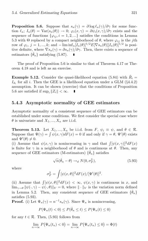
5.4. Generalized Estimating Equations 321
Proposition 5.6. Suppose that sn(γ) = ∂ log n(γ)/∂γ for some func-tion n; In(θ) = Var(sn(θ)) → 0; ϕi(x, γ) = ∂ψi(x, γ)/∂γ exists and thesequence of functions ϕij , i = 1, 2, ... satisfies the conditions in Lemma5.3 with Θ replaced by a compact neighborhood of θ, where ϕij is the jthrow of ϕi, j = 1, ..., k; and − lim infn[In(θ)]1/2E[∇sn(θ)][In(θ)]1/2 is posi-tive definite, where ∇sn(γ) = ∂sn(γ)/∂γ. Then, there exists a sequence ofestimators θn satisfying (5.87).
The proof of Proposition 5.6 is similar to that of Theorem 4.17 or The-orem 4.18 and is left as an exercise.
Example 5.12. Consider the quasi-likelihood equation (5.84) with Ri =Idi for all i. Then the GEE is a likelihood equation under a GLM (§4.4.2)assumption. It can be shown (exercise) that the conditions of Proposition5.6 are satisfied if supi ‖Zi‖ < ∞.
5.4.3 Asymptotic normality of GEE estimators
Asymptotic normality of a consistent sequence of GEE estimators can beestablished under some conditions. We first consider the special case whereθ is univariate and X1, ..., Xn are i.i.d.
Theorem 5.13. Let X1, ..., Xn be i.i.d. from F , ψi ≡ ψ, and θ ∈ R.Suppose that Ψ(γ) =
∫ψ(x, γ)dF (x) = 0 if and only if γ = θ, Ψ′(θ) exists
and Ψ′(θ) = 0.(i) Assume that ψ(x, γ) is nonincreasing in γ and that
∫[ψ(x, γ)]2dF (x)
is finite for γ in a neighborhood of θ and is continuous at θ. Then, anysequence of GEE estimators (M-estimators) θn satisfies
√n(θn − θ) →d N(0, σ2
F ), (5.93)
whereσ2F =
∫[ψ(x, θ)]2dF (x)/[Ψ′(θ)]2.
(ii) Assume that∫
[ψ(x, θ)]2dF (x) < ∞, ψ(x, γ) is continuous in x, andlimγ→θ ‖ψ(·, γ) − ψ(·, θ)‖V = 0, where ‖ · ‖V is the variation norm definedin Lemma 5.2. Then, any consistent sequence of GEE estimators θnsatisfies (5.93).Proof. (i) Let Ψn(γ) = n−1sn(γ). Since Ψn is nonincreasing,
P (Ψn(t) < 0) ≤ P (θn ≤ t) ≤ P (Ψn(t) ≤ 0)
for any t ∈ R. Then, (5.93) follows from
limn→∞
P(Ψn(tn) < 0
)= lim
n→∞P(Ψn(tn) ≤ 0
)= Φ(t)
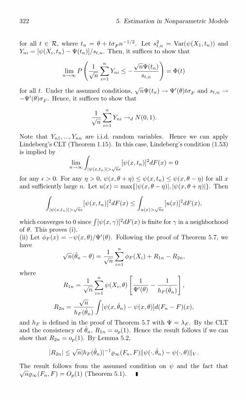
322 5. Estimation in Nonparametric Models
for all t ∈ R, where tn = θ + tσFn−1/2. Let s2
t,n = Var(ψ(X1, tn)) andYni = [ψ(Xi, tn) − Ψ(tn)]/st,n. Then, it suffices to show that
limn→∞
P
(1√n
n∑i=1
Yni ≤ −√nΨ(tn)st,n
)= Φ(t)
for all t. Under the assumed conditions,√nΨ(tn) → Ψ′(θ)tσF and st,n →
−Ψ′(θ)σF . Hence, it suffices to show that
1√n
n∑i=1
Yni →d N(0, 1).
Note that Yn1, ..., Ynn are i.i.d. random variables. Hence we can applyLindeberg’s CLT (Theorem 1.15). In this case, Lindeberg’s condition (1.53)is implied by
limn→∞
∫|ψ(x,tn)|>√
nε
[ψ(x, tn)]2dF (x) = 0
for any ε > 0. For any η > 0, ψ(x, θ + η) ≤ ψ(x, tn) ≤ ψ(x, θ − η) for all xand sufficiently large n. Let u(x) = max|ψ(x, θ− η)|, |ψ(x, θ + η)|. Then∫
|ψ(x,tn)|>√nε
[ψ(x, tn)]2dF (x) ≤∫u(x)>
√nε
[u(x)]2dF (x),
which converges to 0 since∫
[ψ(x, γ)]2dF (x) is finite for γ in a neighborhoodof θ. This proves (i).(ii) Let φF (x) = −ψ(x, θ)/Ψ′(θ). Following the proof of Theorem 5.7, wehave
√n(θn − θ) =
1√n
n∑i=1
φF (Xi) + R1n −R2n,
where
R1n =1√n
n∑i=1
ψ(Xi, θ)
[1
Ψ′(θ)− 1
hF (θn)
],
R2n =√n
hF (θn)
∫[ψ(x, θn) − ψ(x, θ)]d(Fn − F )(x),
and hF is defined in the proof of Theorem 5.7 with Ψ = λF . By the CLTand the consistency of θn, R1n = op(1). Hence the result follows if we canshow that R2n = op(1). By Lemma 5.2,
|R2n| ≤√n|hF (θn)|−1∞(Fn, F )‖ψ(·, θn) − ψ(·, θ)‖V .
The result follows from the assumed condition on ψ and the fact that√n∞(Fn, F ) = Op(1) (Theorem 5.1).
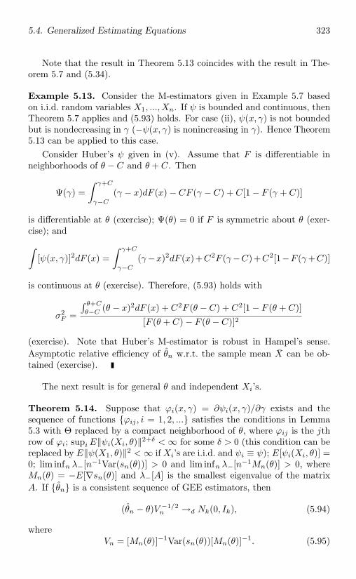
5.4. Generalized Estimating Equations 323
Note that the result in Theorem 5.13 coincides with the result in The-orem 5.7 and (5.34).
Example 5.13. Consider the M-estimators given in Example 5.7 basedon i.i.d. random variables X1, ..., Xn. If ψ is bounded and continuous, thenTheorem 5.7 applies and (5.93) holds. For case (ii), ψ(x, γ) is not boundedbut is nondecreasing in γ (−ψ(x, γ) is nonincreasing in γ). Hence Theorem5.13 can be applied to this case.
Consider Huber’s ψ given in (v). Assume that F is differentiable inneighborhoods of θ − C and θ + C. Then
Ψ(γ) =∫ γ+C
γ−C
(γ − x)dF (x) − CF (γ − C) + C[1 − F (γ + C)]
is differentiable at θ (exercise); Ψ(θ) = 0 if F is symmetric about θ (exer-cise); and∫
[ψ(x, γ)]2dF (x) =∫ γ+C
γ−C
(γ−x)2dF (x)+C2F (γ−C)+C2[1−F (γ+C)]
is continuous at θ (exercise). Therefore, (5.93) holds with
σ2F =
∫ θ+C
θ−C(θ − x)2dF (x) + C2F (θ − C) + C2[1 − F (θ + C)]
[F (θ + C) − F (θ − C)]2
(exercise). Note that Huber’s M-estimator is robust in Hampel’s sense.Asymptotic relative efficiency of θn w.r.t. the sample mean X can be ob-tained (exercise).
The next result is for general θ and independent Xi’s.
Theorem 5.14. Suppose that ϕi(x, γ) = ∂ψi(x, γ)/∂γ exists and thesequence of functions ϕij , i = 1, 2, ... satisfies the conditions in Lemma5.3 with Θ replaced by a compact neighborhood of θ, where ϕij is the jthrow of ϕi; supi E‖ψi(Xi, θ)‖2+δ < ∞ for some δ > 0 (this condition can bereplaced by E‖ψ(X1, θ)‖2 < ∞ if Xi’s are i.i.d. and ψi ≡ ψ); E[ψi(Xi, θ)] =0; lim infn λ−[n−1Var(sn(θ))] > 0 and lim infn λ−[n−1Mn(θ)] > 0, whereMn(θ) = −E[∇sn(θ)] and λ−[A] is the smallest eigenvalue of the matrixA. If θn is a consistent sequence of GEE estimators, then
(θn − θ)V −1/2n →d Nk(0, Ik), (5.94)
whereVn = [Mn(θ)]−1Var(sn(θ))[Mn(θ)]−1. (5.95)
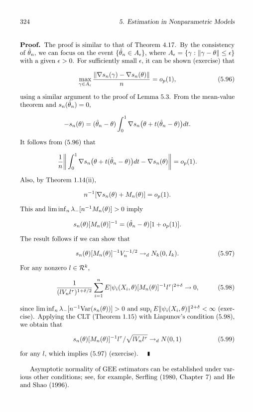
324 5. Estimation in Nonparametric Models
Proof. The proof is similar to that of Theorem 4.17. By the consistencyof θn, we can focus on the event θn ∈ Aε, where Aε = γ : ‖γ − θ‖ ≤ εwith a given ε > 0. For sufficiently small ε, it can be shown (exercise) that
maxγ∈Aε
‖∇sn(γ) −∇sn(θ)‖n
= op(1), (5.96)
using a similar argument to the proof of Lemma 5.3. From the mean-valuetheorem and sn(θn) = 0,
−sn(θ) = (θn − θ)∫ 1
0∇sn
(θ + t(θn − θ)
)dt.
It follows from (5.96) that
1n
∥∥∥∥∫ 1
0∇sn
(θ + t(θn − θ)
)dt−∇sn(θ)
∥∥∥∥ = op(1).
Also, by Theorem 1.14(ii),
n−1[∇sn(θ) + Mn(θ)] = op(1).
This and lim infn λ−[n−1Mn(θ)] > 0 imply
sn(θ)[Mn(θ)]−1 = (θn − θ)[1 + op(1)].
The result follows if we can show that
sn(θ)[Mn(θ)]−1V −1/2n →d Nk(0, Ik). (5.97)
For any nonzero l ∈ Rk,
1(lVnlτ )1+δ/2
n∑i=1
E|ψi(Xi, θ)[Mn(θ)]−1lτ |2+δ → 0, (5.98)
since lim infn λ−[n−1Var(sn(θ))] > 0 and supi E‖ψi(Xi, θ)‖2+δ < ∞ (exer-cise). Applying the CLT (Theorem 1.15) with Liapunov’s condition (5.98),we obtain that
sn(θ)[Mn(θ)]−1lτ/√lVnlτ →d N(0, 1) (5.99)
for any l, which implies (5.97) (exercise).
Asymptotic normality of GEE estimators can be established under var-ious other conditions; see, for example, Serfling (1980, Chapter 7) and Heand Shao (1996).
5.5. Variance Estimation 325
If Xi’s are i.i.d. and ψi ≡ ψ, the asymptotic covariance matrix in (5.95)reduces to
Vn = n−1E[ϕ(X1, θ)]−1E[ψ(X1, θ)]τ [ψ(X1, θ)]E[ϕ(X1, θ)]−1,
where ϕ(x, γ) = ∂ψ(x, γ)/∂γ. When θ is univariate, Vn further reduces to
Vn = n−1E[ψ(X1, θ)]2/E[ϕ(X1, θ)]2.
Under the conditions of Theorem 5.14,
E[ϕ(X1, θ)] =∫
∂ψ(x, θ)∂θ
dF (x) =∂
∂θ
∫ψ(x, θ)dF (x).
Hence, the result in Theorem 5.14 coincides with that in Theorem 5.13.
Example 5.14. Consider the quasi-likelihood equation in (5.84) and ψi in(5.91). If supi ‖Zi‖ < ∞, then ψi satisfies the conditions in Theorem 5.14(exercise). Let Vn(γ) = [Di(γ)]1/2Ri[Di(γ)]1/2. Then
Var(sn(θ)) =n∑
i=1
[Gi(θ)]τ [Vn(θ)]−1Var(Xi)[Vn(θ)]−1Gi(θ)
and
Mn(θ) =n∑
i=1
[Gi(θ)]τ [Vn(θ)]−1Gi(θ).
If Ri = Ri (the true correlation matrix) for all i, then
Var(sn(θ)) =n∑
i=1
φi[Gi(θ)]τ [Vn(θ)]−1Gi(θ).
If, in addition, φi ≡ φ, then
Vn = [Mn(θ)]−1Var(sn(θ))[Mn(θ)]−1 = φ[Mn(θ)]−1.
5.5 Variance Estimation
In statistical inference the accuracy of a point estimator is usually assessedby its mse or amse. If the bias or asymptotic bias of an estimator is (asymp-totically) negligible w.r.t. its mse or amse, then assessing the mse or amse isequivalent to assessing variance or asymptotic variance. Since variances andasymptotic variances usually depend on the unknown population, we haveto estimate them in order to report accuracies of point estimators. Vari-ance estimation is an important part of statistical inference, not only for
326 5. Estimation in Nonparametric Models
assessing accuracy, but also for constructing inference procedures studiedin Chapters 6 and 7. See also the discussion at the end of §2.5.1.
If the unknown population is in a parametric family indexed by a pa-rameter θ, then the covariance matrix or asymptotic covariance matrix ofan estimator of θ is a function of θ, say Vn(θ). If θ is estimated by θ,then it is natural to estimate Vn(θ) by Vn(θ). Thus, variance estimationin parametric problems is usually simple. This idea of substitution can beapplied to nonparametric problems in which variance estimation is muchmore complex.
We introduce three commonly used variance estimation methods in thissection, the substitution method, the jackknife, and the bootstrap.
5.5.1 The substitution method
Suppose that we can obtain a formula for the covariance or asymptoticcovariance matrix of an estimator θn. Then a direct method of varianceestimation is to substitute unknown quantities in the variance formula bysome estimators. To illustrate, consider the simplest case where X1, ..., Xn
are i.i.d. random d-vectors, θn = g(X), and g is a function from Rd to Rk.Suppose that E‖X1‖2 < ∞ and g is differentiable at µ = E(X1). Then, bythe CLT and Theorem 1.12(i),
(θn − θ)V −1/2n →d Nk(0, Ik), (5.100)
where θ = g(µ) and
Vn = ∇g(µ)Var(X1)[∇g(µ)]τ/n (5.101)
is the asymptotic covariance matrix of θn which depends on unknown quan-tities µ and Var(X1). A substitution estimator of Vn is
Vn = ∇g(X)S2[∇g(X)]τ/n, (5.102)
where S2 = (n − 1)−1 ∑ni=1(Xi − X)τ (Xi − X) is the sample covariance
matrix, an extension of the sample variance to the multivariate Xi’s.An essential asymptotic requirement in variance estimation is the con-
sistency of variance estimators according to the following definition.
Definition 5.4. Let Vn be a sequence of k× k positive definite matricesand Vn be an estimator of Vn for each n. Then Vn or Vn is said to beconsistent for Vn if and only if
lVnlτ/lVnl →p 1 for any l ∈ Rk. (5.103)
Vn is strongly consistent if (5.103) holds with →p replaced by →a.s..
5.5. Variance Estimation 327
If (5.103) holds, then (θn − θ)V −1/2n →d Nk(0, Ik), a result useful for
asymptotic inference as discussed in Chapters 6 and 7.By the SLLN, Vn in (5.102) is strongly consistent for Vn in (5.101),
provided that ∇g(µ) = 0 and ∇g is continuous at µ so that ∇g(X) →a.s.
∇g(µ).
Example 5.15. Let Y1, ..., Yn be i.i.d. random variables with finite µy =EY1, σ2
y = Var(Y1), γy = EY 31 , and κy = EY 4
1 . Consider the estimationof θ = (µy, σ
2y). Let θn = (X, σ2
y), where σ2y = n−1 ∑n
i=1(Yi − Y )2. IfXi = (Yi, Y
2i ), then θn = g(X) with g(x) = (x1, x2 − x2
1). Hence, (5.100)holds with
Var(X1) =(
σ2y γy − µy(σ2
y + µ2y)
γy − µy(σ2y + µ2
y) κy − (σ2y + µ2
y)2
)and
∇g(x) =(
1 0−2x1 1
).
The estimator Vn in (5.102) is strongly consistent, since ∇g(x) is obviouslya continuous function.
Similar results can be obtained for problems in Examples 3.21 and 3.23,and Exercises 92 and 93 in §3.6.
A key step in the previous discussion is the derivation of formula (5.101)for the asymptotic covariance matrix of θn = g(X), via Taylor’s expansion(Theorem 1.12) and the CLT. Thus, the idea can be applied to the casewhere θn = T(Fn), a differentiable statistical functional.
We still consider i.i.d. random d-vectors X1, ..., Xn from F . Supposethat T is a vector-valued functional whose components are -Hadamarddifferentiable at F , where is either ∞ or a distance satisfying (5.35).Let φF be the vector of influence functions of components of T. If thecomponents of φF satisfy (5.33), then (5.100) holds with θ = T(F ), θn =T(Fn), Fn = the empirical c.d.f. in (5.1), and
Vn =Var(φF (X1))
n=
1n
∫[φF (x)]τφF (x)dF (x). (5.104)
Formula (5.104) leads to a natural substitution variance estimator
Vn =1n
∫[φFn(x)]τφFn(x)dFn(x) =
1n2
n∑i=1
[φFn(Xi)]τφFn(Xi), (5.105)
provided that φFn(x) is well defined, i.e., the components of T are Gateauxdifferentiable at Fn for sufficiently large n. Under some more conditions onφFn we can establish the consistency of Vn in (5.105).
328 5. Estimation in Nonparametric Models
Theorem 5.15. Let X1, ..., Xn be i.i.d. random d-vectors from F , T bea vector-valued functional whose components are Gateaux differentiable atF and Fn, and φF be the vector of influence functions of components ofT. Suppose that sup‖x‖≤c ‖φFn
(x) − φF (x)‖ = op(1) for any c > 0 andthat there exist a constant c0 > 0 and a function h(x) ≥ 0 such thatE[h(X1)] < ∞ and P
(sup‖x‖≥c0 ‖φFn(x)‖2 ≤ h(x)
)→ 1. Then Vn in
(5.105) is consistent for Vn in (5.104).Proof. Let ζ(x) = [φF (x)]τ [φF (x)] and ζn(x) = [φFn(x)]τ [φFn(x)]. By theSLLN,
1n
n∑i=1
ζ(Xi) →a.s.
∫ζ(x)dF (x).
Hence the result follows from
1n
n∑i=1
[ζn(Xi) − ζ(Xi)] = op(1).
Using the assumed conditions and the argument in the proof of Lemma 5.3,we can show that for any ε > 0, there is a c > 0 such that
P
(1n
n∑i=1
‖ζn(Xi) − ζ(Xi)‖I(c,∞)(‖Xi‖) >ε
2
)≤ ε
and
P
(1n
n∑i=1
‖ζn(Xi) − ζ(Xi)‖I[0,c](‖Xi‖) >ε
2
)≤ ε
for sufficiently large n. This completes the proof.
Example 5.16. Consider the L-functional defined in (5.39) and the L-estimator θn = T(Fn). Theorem 5.6 shows that T is Hadamard differentiableat F under some conditions on J . It can be shown (exercise) that T isGateaux differentiable at Fn with φFn(x) given by (5.41) (with F replacedby Fn). Then the difference φFn(x) − φF (x) is equal to∫
(Fn − F )(y)J(Fn(y))dy +∫
(F − δx)(y)[J(Fn(y)) − J(F (y))]dy.
One can show (exercise) that the conditions in Theorem 5.15 are satisfiedif the conditions in Theorem 5.6(i) or (ii) (with E|X1| < ∞) hold.
Substitution variance estimators for M-estimators and U-statistics canalso be derived (exercises).
The substitution method can clearly be applied to non-i.i.d. cases. Forexample, the LSE β in linear model (3.25) with a full rank Z and i.i.d. εi’s
5.5. Variance Estimation 329
has Var(β) = σ2(ZτZ)−1, where σ2 = Var(ε1). A consistent substitutionestimator of Var(β) can be obtained by replacing σ2 in the formula of Var(β)by a consistent estimator of σ2 such as SSR/(n− p) (see (3.36)).
We now consider variance estimation for the GEE estimators describedin §5.4.1. By Theorem 5.14, the asymptotic covariance matrix of the GEEestimator θn is given by (5.95), where
Var(sn(θ)) =n∑
i=1
E[ψi(Xi, θ)]τψi(Xi, θ),
Mn(θ) =n∑
i=1
E[ϕi(Xi, θ)],
and ϕi(x, γ) = ∂ψi(x, γ)/∂γ. Substituting θ by θn and the expectationsby their empirical analogues, we obtain the substitution estimator Vn =M−1
n Var(sn)M−1n , where
Var(sn) =n∑
i=1
[ψi(Xi, θn)]τψi(Xi, θn)
and
Mn =n∑
i=1
ϕi(Xi, θn).
The proof of the following result is left as an exercise.
Theorem 5.16. Let X1, ..., Xn be independent and θn be a consistentsequence of GEE estimators. Assume the conditions in Theorem 5.14. Sup-pose further that the sequence of functions hij , i = 1, 2, ... satisfies theconditions in Lemma 5.3 with Θ replaced by a compact neighborhood ofθ, where hij(x, γ) is the jth row of [ψi(x, γ)]τψi(x, γ). Let Vn be given by(5.95). Then Vn = M−1
n Var(sn)M−1n is consistent for Vn.
5.5.2 The jackknife
Applying the substitution method requires the derivation of a formula forthe covariance matrix or asymptotic covariance matrix of a point estimator.There are variance estimation methods that can be used without actuallyderiving such a formula (only the existence of the covariance matrix orasymptotic covariance matrix is assumed), at the expense of requiring alarge number of computations. These methods are called resampling meth-ods, replication methods, or data reuse methods. The jackknife methodintroduced here and the bootstrap method in §5.5.3 are the most popularresampling methods.
330 5. Estimation in Nonparametric Models
The jackknife method was proposed by Quenouille (1949) and Tukey(1958). Let θn be a vector-valued estimator based on independent Xi’s,where each Xi is a random di-vector and supi di < ∞. Let θ−i be thesame estimator but based on X1, ..., Xi−1, Xi+1, ..., Xn, i = 1, ..., n. Notethat θ−i also depends on n but the subscript n is omitted for simplicity.Since θn and θ−1, ..., θ−n are estimators of the same quantity, the “samplecovariance matrix”
1n− 1
n∑i=1
(θ−i − θn
)τ (θ−i − θn
)(5.106)
can be used as a measure of the variation of θn, where θn is the average ofθ−i’s.
There are two major differences between the quantity in (5.106) andthe sample covariance matrix S2 previously discussed. First, θ−i’s are notindependent. Second, θ−i − θ−j usually converges to 0 at a fast rate (suchas n−1). Hence, to estimate the asymptotic covariance matrix of θn, thequantity in (5.106) should be multiplied by a correction factor cn. If θn = X
(di ≡ d), then θ−i = (n−1)−1(X−Xi) and the quantity in (5.106) reducesto
1(n− 1)3
n∑i=1
(Xi − X
)τ (Xi − X
)=
1(n− 1)2
S2,
where S2 is the sample covariance matrix. Thus, the correction factor cn is(n− 1)2/n for the case of θn = X, since, by the SLLN, S2/n is consistentfor Var(X).
It turns out that the same correction factor works for many other esti-mators. This leads to the following jackknife variance estimator for θn:
VJ =n− 1n
n∑i=1
(θ−i − θn
)τ (θ−i − θn
). (5.107)
Theorem 5.17. Let X1, ..., Xn be i.i.d. random d-vectors from F withfinite µ = E(X1) and Var(X1), and let θn = g(X). Suppose that ∇g iscontinuous at µ and ∇g(µ) = 0. Then the jackknife variance estimator VJ
in (5.107) is strongly consistent for Vn in (5.101).Proof. From Definition 5.4, it suffices to show the case where g is real-valued. Let X−i be the sample mean based on X1, ..., Xi−1, Xi+1, ..., Xn.From the mean-value theorem, we have
θ−i − θn = g(X−i) − g(X)= ∇g(ξn,i)(X−i − X)τ
= ∇g(X)(X−i − X)τ + Rn,i,
5.5. Variance Estimation 331
where Rn,i =[∇g(ξn,i) − ∇g(X)
](X−i − X)τ and ξn,i is a point on the
line segment between X−i and X. From X−i − X = (n− 1)−1(X −Xi), itfollows that
∑ni=1(X−i − X) = 0 and
1n
n∑i=1
(θ−i − θn) =1n
n∑i=1
Rn,i = Rn.
From the definition of the jackknife estimator in (5.107),
VJ = An + Bn + 2Cn,
where
An =n− 1n
∇g(X)n∑
i=1
(X−i − X)τ (X−i − X)[∇g(X)]τ ,
Bn =n− 1n
n∑i=1
(Rn,i − Rn)2
and
Cn =n− 1n
n∑i=1
(Rn,i − Rn)∇g(X)(X−i − X)τ .
By X−i − X = (n− 1)−1(X −Xi), the SLLN, and the continuity of ∇g atµ,
An/Vn →a.s. 1.
Also,
(n− 1)n∑
i=1
‖X−i − X‖2 =1
n− 1
n∑i=1
‖Xi − X‖2 = O(1) a.s. (5.108)
Hencemaxi≤n
‖X−i − X‖2 →a.s. 0,
which, together with the continuity of ∇g at µ and ‖ξn,i−X‖ ≤ ‖X−i−X‖,implies that
un = maxi≤n
‖∇g(ξn,i) −∇g(X)‖ →a.s. 0.
From (5.101) and (5.108),∑n
i=1 ‖X−i − X‖2/Vn = O(1) a.s. Hence
Bn
Vn≤ n− 1
Vnn
n∑i=1
R2n,i ≤
un
Vn
n∑i=1
‖X−i − X‖2 →a.s. 0.
By the Cauchy-Schwarz inequality, (Cn/Vn)2 ≤ (An/Vn)(Bn/Vn) →a.s. 0.This proves the result.
332 5. Estimation in Nonparametric Models
A key step in the proof of Theorem 5.17 is that θ−i − θn can be ap-proximated by ∇g(X)(X−i− X)τ and the contributions of the remainders,Rn,1, ..., Rn,n, are sufficiently small, i.e., Bn/Vn →a.s. 0. This indicatesthat the jackknife estimator (5.107) is consistent for θn that can be well ap-proximated by some linear statistic. In fact, the jackknife estimator (5.107)has been shown to be consistent when θn is a U-statistic (Arvesen, 1969)or a statistical functional that is Hadamard differentiable and continuouslyGateaux differentiable at F (which includes certain types of L-estimatorsand M-estimators). More details can be found in Shao and Tu (1995, Chap-ter 2).
The jackknife method can be applied to non-i.i.d. problems. A detaileddiscussion of the use of the jackknife method in survey problems can befound in Shao and Tu (1995, Chapter 6). We now consider the jackknifevariance estimator for the LSE β in linear model (3.25). For simplicity,assume that Z is of full rank. Assume also that εi’s are independent withE(εi) = 0 and Var(εi) = σ2
i . Then
Var(β) = (ZτZ)−1n∑
i=1
σ2iZ
τi Zi(ZτZ)−1.
Let β−i be the LSE of β based on the data with the ith pair (Xi, Zi) deleted.Using the fact that (A + cτ c)−1 = A−1 − A−1cτ cA−1/(1 + cA−1cτ ) for amatrix A and a vector c, we can show that (exercise)
β−i = β − riZi/(1 − hii), (5.109)
where ri = Xi − βZτi is the ith residual and hii = Zi(ZτZ)−1Zτ
i . Hence
VJ =n− 1n
(ZτZ)−1
[n∑
i=1
r2iZ
τi Zi
(1 − hii)2− 1
n
n∑i=1
riZτi
1 − hii
n∑i=1
riZi
1 − hii
](ZτZ)−1.
Wu (1986) proposed the following weighted jackknife variance estimatorthat improves VJ :
VWJ =n∑
i=1
(1−hii)(β−i − β
)τ (β−i − β
)= (ZτZ)−1
n∑i=1
r2iZ
τi Zi
1 − hii(ZτZ)−1.
Theorem 5.18. Assume the conditions in Theorem 3.12 and that εi’s areindependent. Then both VJ and VWJ are consistent for Var(β).Proof. Let l ∈ Rp be a fixed nonzero vector and li = l(ZτZ)−1Zτ
i . Sincemaxi≤n hii → 0, the result for VWJ follows from
n∑i=1
l2i r2i
/ n∑i=1
l2i σ2i →p 1. (5.110)
5.5. Variance Estimation 333
By the WLLN (Theorem 1.14(ii)),n∑
i=1
l2i ε2i
/ n∑i=1
l2i σ2i →p 1.
Note that ri = εi + (β − β)Zτi and
maxi≤n
[(β − β)Zτi ]2 ≤ ‖(β − β)Zτ‖2 max
i≤nhii = op(1).
Hence (5.110) holds.The consistency of VJ follows from (5.110) and
n− 1n2
(n∑
i=1
liri1 − hii
)2 / n∑i=1
l2i σ2i = op(1). (5.111)
The proof of (5.111) is left as an exercise.
Finally, let us consider the jackknife estimators for GEE estimators in§5.4.1. Under the conditions of Proposition 5.5 or 5.6, it can be shown that
maxi≤n
‖θ−i − θ‖ = op(1), (5.112)
where θ−i is a root of sni(γ) = 0 and
sni(γ) =∑
j =i,j≤n
ψj(Xj , γ).
Using Taylor’s expansion and the fact that sni(θ−i) = 0 and sn(θn) = 0,we obtain that
ψi(Xi, θ−i) = (θ−i − θn)∫ 1
0∇sn
(θn + t(θ−i − θn)
)dt.
Following the proof of Theorem 5.14, we obtain that
VJ = [Mn(θ)]−1n∑
i=1
[ψi(Xi, θ−i)]τψi(Xi, θ−i)[Mn(θ)]−1 + Rn,
where Rn denotes a quantity satisfying lRnlτ/lVnl
τ = op(1) for Vn in (5.95).Under the conditions of Theorem 5.16, it follows from (5.112) that VJ isconsistent.
If θn is computed using an iteration method, then the computation ofVJ requires n additional iteration processes. We may use the idea of aone-step MLE to reduce the amount of computation. For each i, let
θ−i = θn − sni(θn)[∇sni(θn)]−1, (5.113)
334 5. Estimation in Nonparametric Models
which is the result from the first iteration when Newton-Raphson’s methodis applied in computing a root of sni(γ) = 0 and θn is used as the initialpoint. Note that θ−i’s in (5.113) satisfy (5.112) (exercise). If the jackknifevariance estimator is based on θ−i’s in (5.113), then
VJ = [Mn(θ)]−1n∑
i=1
[ψi(Xi, θn)]τψi(Xi, θn)[Mn(θ)]−1 + Rn.
These results are summarized in the following theorem.
Theorem 5.19. Assume the conditions in Theorems 5.14 and 5.16. As-sume further that θ−i’s are given by (5.113) or GEE estimators satisfying(5.112). Then the jackknife variance estimator VJ is consistent for Vn givenin (5.95).
5.5.3 The bootstrap
The basic idea of the bootstrap method can be described as follows. Sup-pose that P is a population or model that generates the sample X and thatwe need to estimate Var(θ), where θ = θ(X) is an estimator, a statisticbased on X. Suppose further that the unknown population P is estimatedby P , based on the sample X. Let X∗ be a sample (called a bootstrapsample) taken from the estimated population P using the same or a similarsampling procedure used to obtain X, and let θ∗ = θ(X∗), which is thesame as θ but with X replaced by X∗. If we believe that P = P (i.e.,we have a perfect estimate of the population), then Var(θ) = Var∗(θ∗),where Var∗ is the conditional variance w.r.t. the randomness in generatingX∗, given X. In general, P = P and, therefore, Var(θ) = Var∗(θ∗). ButVB = Var∗(θ∗) is an empirical analogue of Var(θ) and can be used as anestimate of Var(θ).
In a few cases, an explicit form of VB = Var∗(θ∗) can be obtained.First, consider i.i.d. X1, ..., Xn from a c.d.f. F on Rd. The population isdetermined by F . Suppose that we estimate F by the empirical c.d.f. Fn
in (5.1) and that X∗1 , ..., X
∗n are i.i.d. from Fn. For θ = X, its bootstrap
analogue is θ∗ = X∗, the average of X∗i ’s. Then
VB = Var∗(X∗) =1n2
n∑i=1
(Xi − X)τ (Xi − X) =n− 1n2 S2,
where S2 is the sample covariance matrix. In this case VB = Var∗(X∗) isa strongly consistent estimator for Var(X). Next, consider i.i.d. randomvariables X1, ..., Xn from a c.d.f. F on R and θ = F−1
n ( 12 ), the sample
5.5. Variance Estimation 335
median. Suppose that n = 2l − 1 for an integer l. Let X∗1 , ..., X
∗n be i.i.d.
from Fn and θ∗ be the sample median based on X∗1 , ..., X
∗n. Then
VB = Var∗(θ∗) =n∑
j=1
pj
(X(j) −
n∑i=1
piX(i)
)2
,
where X(1) ≤ · · · ≤ X(n) are order statistics and pj = P (θ∗ = X(j)|X). Itcan be shown (exercise) that
pj =l−1∑t=0
(n
t
)(j − 1)t(n− j + 1)n−t − jt(n− j)n−t
nn. (5.114)
However, in most cases VB does not have a simple explicit form. WhenP is known, the Monte Carlo method described in §4.1.4 can be used toapproximate Var(θ). That is, we draw repeatedly new data sets from P andthen use the sample covariance matrix based on the values of θ computedfrom new data sets as a numerical approximation to Var(θ). This ideacan be used to approximate VB , since P is a known population. That is,we can draw m bootstrap data sets X∗1, ..., X∗m independently from P(conditioned on X), compute θ∗j = θ(X∗j), j = 1, ...,m, and approximateVB by
V mB =
1m
m∑j=1
(θ∗j − θ∗
)τ (θ∗j − θ∗
),
where θ∗ is the average of θ∗j ’s. Since each X∗j is a data set generated fromP , V m
B is a resampling estimator. From the SLLN, as m → ∞, V mB →a.s.
VB , conditioned on X. Both VB and its Monte Carlo approximation V mB are
called bootstrap variance estimators for θ. V mB is more useful in practical
applications, whereas in theoretical studies, we usually focus on VB .The consistency of the bootstrap variance estimator VB is a much more
complicated problem than that of the jackknife variance estimator in §5.5.2.Some examples can be found in Shao and Tu (1995, §3.2.2).
The bootstrap method can also be applied to estimate quantities otherthan Var(θ). For example, let K(t) = P (θ ≤ t) be the c.d.f. of a real-valuedestimator θ. From the previous discussion, a bootstrap estimator of K(t)is the conditional probability P (θ∗ ≤ t|X), which can be approximatedby the Monte Carlo approximation m−1 ∑m
j=1 I(−∞,t](θ∗j). An importantapplication of bootstrap distribution estimators in problems of constructingconfidence sets is studied in §7.4. Here, we study the use of a bootstrapdistribution estimator to form a consistent estimator of the asymptoticvariance of a real-valued estimator θ.
336 5. Estimation in Nonparametric Models
Suppose that √n(θ − θ) →d N(0, v), (5.115)
where v is unknown. Let Hn(t) be the c.d.f. of√n(θ − θ) and
HB(t) = P (√n(θ∗ − θ) ≤ t|X) (5.116)
be a bootstrap estimator of Hn(t). If
HB(t) −Hn(t) →p 0
for any t, then, by (5.115),
HB(t) − Φ(t/√v)→p 0,
which implies (exercise) that
H−1B (α) →p Φ−1 (
α/√v)
=√vΦ−1(α)
for any α ∈ (0, 1). Then, for α = 12 ,
H−1B (1 − α) − H−1
B (α) →p
√v[Φ−1(1 − α) − Φ−1(α)].
Therefore, a consistent estimator of v/n, the asymptotic variance of θ, is
VB =1n
[H−1
B (1 − α) − H−1B (α)
Φ−1(1 − α) − Φ−1(α)
]2
.
The following result gives some conditions under which HB(t)−Hn(t) →p 0.The proof of part (i) is omitted. The proof of part (ii) is given in Exercises97-99 in §5.6.
Theorem 5.20. Suppose that X1, ..., Xn are i.i.d. from a c.d.f. F on Rd.Let θ = T(Fn), where T is a real-valued functional, θ∗ = T(F ∗
n), where F ∗n is
the empirical c.d.f. based on a bootstrap sample X∗1 , ..., X
∗n i.i.d. from Fn,
and let HB be given by (5.116).(i) If T is ∞-Hadamard differentiable at F and (5.33) holds, then
∞(HB , Hn) →p 0. (5.117)
(ii) If d = 1 and T is Lp-Frechet differentiable at F (
∫F (t)[1−F (t)]p/2dt
< ∞ if 1 ≤ p < 2) and (5.33) holds, then (5.117) holds.
Applications of the bootstrap method to non-i.i.d. cases can be found,for example, in Efron and Tibshirani (1993), Hall (1992), and Shao and Tu(1995).
5.6. Exercises 337
5.6 Exercises
1. Let ∞ be defined by (5.3).(a) Show ∞ is a distance on F.(b) Find an example of a sequence Gj ⊂ F for which limj→∞ Gj(t)= G0(t) for every t at which G0 is continuous, but ∞(Gj , G0) doesnot converge to 0.
2. Let X1, ..., Xn be i.i.d. random d-vectors with c.d.f. F and Fn be theempirical c.d.f. defined by (5.1). Show that for any t > 0 and ε > 0,there is a Cε,d such that for all n = 1, 2, ...,
P
(supm≥n
∞(Fm, F ) > t
)≤ Cε,de
−(2−ε)t2n
1 − e−(2−ε)t2 .
3. Show that Mpdefined by (5.4) is a distance on Fp, p ≥ 1.
4. Show that Lpdefined by (5.5) is a distance on F1 for any p ≥ 1.
5. Let F1 be the collection of c.d.f.’s on R with finite means.(a) Show that M1
(G1, G2) =∫ 10 |G−1
1 (z)−G−12 (z)|dz, where G−1(z)
= inft : G(t) ≥ z for any G ∈ F.(b) Show that M1
(G1, G2) = L1(G1, G2).
6. Find an example of a sequence Gj ⊂ F for which(a) limj→∞ ∞(Gj , G0) = 0 but M2
(Gj , G0) does not converge to 0;(b) limj→∞ M2
(Gj , G0) = 0 but ∞(Gj , G0) does not converge to 0.
7. Repeat the previous exercise with M2replaced by L2
.
8. Let X be a random variable having c.d.f. F . Show that(a) E|X|2 < ∞ implies
∫F (t)[1 − F (t)]p/2dt < ∞ for p ∈ (1, 2);
(b) E|X|2+δ < ∞ with some δ > 0 implies∫F (t)[1 − F (t)]1/2dt <
∞.
9. For any one-dimensional Gj ∈ F1, j = 1, 2, show that L1(G1, G2) ≥
|∫xdG1 −
∫xdG2|.
10. In the proof of Theorem 5.3, show that pi = c/n, i = 1, ..., n, λ =−(c/n)n−1 is a maximum of the function H(p1, ..., pn, λ) over pi > 0,i = 1, ..., n,
∑ni=1 pi = c.
11. Show that (5.11)-(5.13) is a solution to the problem of maximizing(G) in (5.8) subject to (5.10).
12. In the proof of Theorem 5.4, prove the case of m ≥ 2.
338 5. Estimation in Nonparametric Models
13. Show that a maximum of (G) in (5.17) subject to (5.10) is given by(5.11) with pi defined by (5.18) and (5.19).
14. In Example 5.2, show that an MELE is given by (5.11) with pi’s givenby (5.21).
15. In Example 5.3, show that(a) maximizing (5.22) subject to (5.23) is equivalent to maximizing
n∏i=1
qδ(i)i (1 − qi)n−i+1−δ(i) ,
where qi = pi/∑n+1
j=i pj , i = 1, ..., n;(b) F given by (5.24) maximizes (5.22) subject to (5.23); (Hint: usepart (a) and the fact that pi = qi
∏i−1j=1(1 − qj).)
(c) F given by (5.25) is the same as that in (5.24).(d) if δi = 1 for all i (no censoring), then F in (5.25) is the same asthe empirical c.d.f. in (5.1).
16. Let fn be given by (5.26).(a) Show that fn is a Lebesgue p.d.f. on R.(b) Suppose that f is continuously differentiable at t, λn → 0, andnλn → ∞. Show that (5.27) holds.(c) Under nλ3
n → 0 and the conditions of (b), show that (5.28) holds.(d) Suppose that f is continuous on [a, b], −∞ < a < b < ∞, λn → 0,and nλn → ∞. Show that
∫ b
afn(t)dt →p
∫ b
af(t)dt.
17. Let f be given by (5.29).(a) Show that f is a Lebesgue p.d.f. on R.(b) Prove (5.30) under the condition that λn → 0, nλn → ∞, andf is bounded and is continuous at t and
∫[w(t)]2+δdt < ∞ for some
δ > 0. (Hint: check Liapunov’s condition and apply Theorem 1.15.)(c) Suppose that λn → 0, nλn → ∞, and f is bounded and is contin-uous on [a, b], −∞ < a < b < ∞. Show that
∫ b
af(t)dt →p
∫ b
af(t)dt.
18. Show that -Frechet differentiability implies -Hadamard differentia-bility.
19. Suppose that a functional T is Gateaux differentiable at F with acontinuous differential LF in the sense that ∞(∆j ,∆) → 0 impliesLF (∆j) → LF (∆). Show that φF is bounded.
20. Suppose that a functional T is Gateaux differentiable at F with abounded and continuous influence function φF . Show that the differ-ential LF is continuous in the sense described in the previous exercise.
5.6. Exercises 339
21. Let T(G) = g(∫xdG) be a functional defined on F1, the collection of
one-dimensional c.d.f.’s with finite means.(a) Find a differentiable function g for which the functional T is not∞-Hadamard differentiable at F .(b) Show that if g is a differentiable function, then T is L1
-Frechetdifferentiable at F . (Hint: use the result in Exercise 9.)
22. In Example 5.5, show that (5.36) holds. (Hint: for ∆ = c(G1 −G2),show that ‖∆‖V ≤ |c|(‖G1‖V + ‖G2‖V ) = 2|c|.)
23. In Example 5.5, show that φF is continuous if F is continuous.
24. In Example 5.5, show that T is not ∞-Frechet differentiable at F .
25. Prove Proposition 5.1(ii).
26. Suppose that T is first-order and second-order -Hadamard differen-tiable at F . Prove (5.38).
27. Find an example of a second-order -Frechet differentiable functionalT that is not first-order -Hadamard differentiable.
28. Prove (5.40) and that (5.33) is satisfied if F has a finite variance.
29. Prove (iv) and (v) of Theorem 5.6.
30. Discuss which of (i)-(v) in Theorem 5.6 can be applied to each of theL-estimators in Example 5.6.
31. Obtain explicit forms of the influence functions for L-estimators inExample 5.6. Discuss which of them are bounded and continuous.
32. Provide an example in which the L-functional T given by (5.39) is not∞-Hadamard differentiable at F . (Hint: consider an untrimmed J .)
33. Discuss which M-functionals defined in (i)-(vi) of Example 5.7 satisfythe conditions of Theorem 5.7.
34. In the proof of Theorem 5.7, show that R2j → 0.
35. Show that the second equality in (5.44) holds when ψ is Borel andbounded.
36. Show that the functional T in (5.46) is ∞-Hadamard differentiable atF with the differential given by (5.47). Obtain the influence functionφF and show that it is bounded and continuous if F is continuous.
340 5. Estimation in Nonparametric Models
37. Show that the functional T in (5.48) is ∞-Hadamard differentiableat F with the differential given by (5.49). Obtain the influence func-tion φF and show that it is bounded and continuous if F (y,∞) andF (∞, z) are continuous.
38. Let F be a continuous c.d.f. on R. Suppose that F is symmetricabout θ and is strictly increasing in a neighborhood of θ. Show thatλF (t) = 0 if and only if t = θ, where λF (t) is defined by (5.50) witha strictly increasing J satisfying J(1 − t) = −J(t).
39. Show that λF (t) in (5.50) is differentiable at θ and λ′F (θ) is equal to
−∫J ′(F (x))F ′(x)dF (x).
40. Let T(Fn) be an R-estimator satisfying the conditions in Theorem 5.8.Show that (5.34) holds with
σ2F =
∫ 1
0[J(t)]2dt
/[∫ ∞
−∞J ′(F (x))F ′(x)dF (x)
]2
.
41. Calculate the asymptotic relative efficiency of the Hodges-Lehmannestimator in Example 5.8 w.r.t. the sample mean based on an i.i.d.sample from F when(a) F is the c.d.f. of N(µ, σ2);(b) F is the c.d.f. of the logistic distribution LG(µ, σ);(c) F is the c.d.f. of the double exponential distribution DE(µ, σ);(d) F (x) = F0(x − θ), where F0(x) is the c.d.f. of the t-distributiontν with ν ≥ 3.
42. Let G be a c.d.f. on R. Show that G(x) ≥ t if and only if x ≥ G−1(t).
43. Show that (5.60) implies that θp is strongly consistent for θp and is√n-consistent for θp if F ′(θp−) and F ′(θp+) exist.
44. Under the condition of Theorem 5.9, show that for ρε = e−2δ2ε ,
P
(supm≥n
|θp − θp| > ε
)≤ 2Cρnε
1 − ρε, n = 1, 2, ....
45. Prove that ϕn(t) in (5.62) is the Lebesgue p.d.f. of the pth samplequantile θp when F has the Lebesgue p.d.f. f , by(a) differentiating the c.d.f. of θp in (5.61);(b) using result (5.59) and the result in Example 2.9.
46. Let X1, ..., Xn be i.i.d. random variables from F with a finite mean.Show that θp has a finite jth moment for sufficiently large n, j =1, 2,....
5.6. Exercises 341
47. Prove Theorem 5.10(i).
48. Suppose that a c.d.f. F has a Lebesgue p.d.f. f . Using the p.d.f. in(5.62) and Scheffe’s theorem (Proposition 1.17), prove part (iv) ofTheorem 5.10.
49. Let kn be a sequence of integers satisfying kn/n = p + o(n−1/2)with p ∈ (0, 1), and let X1, ..., Xn be i.i.d. random variables from ac.d.f. F with F ′(θp) > 0. Show that
√n(X(kn) − θp) →d N(0, p(1 − p)/[F ′(θp)]2).
50. In the proof of Theorem 5.11, prove (5.65), (5.68), and inequality(5.67).
51. Prove Corollary 5.1.
52. Prove the claim in Example 5.9.
53. Let T (G) = G−1(p) be the pth quantile functional. Suppose that Fhas a positive derivative F ′ in a neighborhood of θ = F−1(p). Showthat T is Gateaux differentiable at F and obtain the influence functionφF (x).
54. Let X1, ..., Xn be i.i.d. from the Cauchy distribution C(0, 1).(a) Show that E(X(j))2 < ∞ if and only if 3 ≤ j ≤ n− 2.(b) Show that E(θ0.5)2 < ∞ for n ≥ 5.
55. Suppose that F is the c.d.f. of the uniform distribution U(θ− 12 , θ+ 1
2 ),θ ∈ R. Obtain the asymptotic relative efficiency of the sample medianw.r.t. the sample mean, based on an i.i.d. sample of size n from F .
56. Suppose that F (x) = F0(x − θ) and F0 is the c.d.f. of the Cauchydistribution C(0, 1) truncated at c and −c, i.e., F0 has the Lebesguep.d.f. (1 + x2)−1I(−c,c)(x)/
∫ c
−c(1 + x2)−1dt. Obtain the asymptotic
relative efficiency of the sample median w.r.t. the sample mean, basedon an i.i.d. sample of size n from F .
57. Show that Xα in (5.70) is the L-estimator corresponding to the Jfunction given in Example 5.6(iii) with β = 1 − α.
58. Let X1, ..., Xn be i.i.d. random variables from F , where F is symmet-ric about θ.(a) Show that X(j) − θ and θ−X(n−j+1) have the same distribution.(b) Show that
∑nj=1 wjX(j) has a c.d.f. symmetric about θ, if wi’s are
constants satisfying∑n
i=1 wi = 1 and wj = wn−j+1 for all j.(c) Show that the trimmed sample mean Xα has a c.d.f. symmetricabout θ.
342 5. Estimation in Nonparametric Models
59. Under the conditions in one of (i)-(iii) of Theorem 5.6, show that(5.34) holds for T(Fn) with σ2
F given by (5.72), if σ2F < ∞.
60. Prove (5.71) under the assumed conditions.
61. For the functional T given by (5.39), show that T(F ) = θ if F issymmetric about θ and J is symmetric about 1
2 .
62. Suppose that F is the double exponential distribution DE(θ, 1), whereθ ∈ R. Obtain the asymptotic relative efficiency of the trimmed sam-ple mean Xα w.r.t. the sample mean, based on an i.i.d. sample of sizen from F .
63. Show that the method of moments in §3.5.2 is a special case of theGEE method.
64. Let (θ, ξ) be a likelihood. Show that a maximum profile likelihoodestimator θ of θ is an MLE if ξ(θ), the maximum of supξ (θ, ξ) for afixed θ, does not depend on θ.
65. Let X1, ..., Xn be i.i.d. from N(µ, σ2). Derive the profile likelihoodfunction for µ or σ2. Discuss in each case whether the maximumprofile likelihood estimator is the same as the MLE.
66. Complete the proof of Proposition 5.4.
67. In the proof of Lemma 5.3, show that the probability in (5.89) isbounded by ε.
68. In Example 5.11, show that ψi’s satisfy the conditions of Lemma 5.3if Θ is compact and supi ‖Zi‖ < ∞.
69. In the proof of Proposition 5.5, show that ∆n(γ) is equicontinuouson any open subset of Θ.
70. Prove Proposition 5.6.
71. Prove the claim in Example 5.12.
72. Prove the claims in Example 5.13.
73. For Huber’s M-estimator discussed in Example 5.13, obtain a formulafor e(F ), the asymptotic relative efficiency of θn w.r.t. X, when F isgiven by (5.69). Show that limτ→∞ e(F ) = ∞. Find the value ofe(F ) when ε = 0, σ = 1, and C = 1.5.
74. Consider the ψ function in Example 5.7(ii). Show that under someconditions on F , ψ satisfies the conditions given in Theorem 5.13(i)or (ii). Obtain σ2
F in (5.93) in this case.
5.6. Exercises 343
75. In the proof of Theorem 5.14, show that(a) (5.96) holds;(b) (5.98) holds;(c) (5.99) implies (5.97). (Hint: use Theorem 1.9(iii).)
76. Prove the claim in Example 5.14, assuming some necessary momentconditions.
77. Derive the asymptotic distribution of the MQLE (the GEE estima-tor based on (5.84)), assuming that Xi = (Xi1, ..., Xidi), E(Xit) =meηi/(1 + eηi), Var(Xit) = mφie
ηi/(1 + eηi)2, and (4.57) holds withg(t) = log t
1−t .
78. Repeat the previous exercise under the assumption that E(Xit) = eηi ,Var(Xit) = φie
ηi , and (4.57) holds with g(t) = log t or g(t) = 2√t.
79. In Theorem 5.14, show that result (5.94) still holds if Ri is replacedby an estimator Ri satisfying maxi≤n ‖Ri − Ui‖ = op(1), where Ui’sare correlation matrices.
80. Suppose that X1, ..., Xn are independent (not necessarily identicallydistributed) random d-vectors with E(Xi) = µ for all i. Suppose alsothat supi E‖Xi‖2+δ < ∞ for some δ > 0. Let µ = E(X1), θ = g(µ),and θn = g(X). Show that(a) (5.100) holds with Vn = n−2∇g(µ)
∑ni=1 Var(Xi)[∇g(µ)]τ ;
(b) Vn in (5.102) is consistent for Vn in part (a).
81. Consider the ratio estimator in Example 3.21. Derive the estimatorVn given by (5.102) and show that Vn is consistent for the asymptoticvariance of the ratio estimator.
82. Derive a consistent variance estimator for R(t) in Example 3.23.
83. Prove the claims in Example 5.16.
84. Derive a consistent variance estimator for a U-statistic satisfying theconditions in Theorem 3.5(i).
85. Derive a consistent variance estimator for Huber’s M-estimator dis-cussed in Example 5.13.
86. Assume the conditions in Theorem 5.8. Let r ∈ (0, 12 ).
(a) Show that nrλF (T(Fn) + n−r) →p λF (T(F )).(b) Show that nr[λFn
(T(Fn) + n−r) − λF (T(Fn) + n−r)] →p 0.(c) Derive a consistent estimator of the asymptotic variance of T(Fn),using the results in (a) and (b).
87. Prove Theorem 5.16.
344 5. Estimation in Nonparametric Models
88. Let X1, ..., Xn be random variables and θ = X2. Show that thejackknife estimator in (5.107) equals 4X2c2
n−1 − 4Xc3(n−1)2 + c4−c22
(n−1)3 , wherecj ’s are the sample central moments defined by (3.57).
89. Prove (5.109).
90. In the proof of Theorem 5.18, prove (5.111).
91. Show that θ−i’s in (5.113) satisfy (5.112), under the conditions ofTheorem 5.14.
92. Prove Theorem 5.19.
93. Prove (5.114).
94. Let X1, ..., Xn be random variables and θ = X2. Show that thebootstrap variance estimator based on i.i.d. X∗
i ’s from Fn is equal toVB = 4X2c2
n + 4Xc3n2 + c4
n3 , where cj ’s are the sample central momentsdefined by (3.57).
95. Let X1, ..., Xn be i.i.d. from a Lebesgue p.d.f. 1σf
(x−µσ
)on R, where
f is known. Let Hn(t) = P (√n(X − µ)/S ≤ t) and HB(t) =
P (√n(X∗ − X)/S∗ ≤ t|X) be the bootstrap estimator of Hn, where
S2 is the sample variance, X∗i ’s are i.i.d. from 1
sf(x−xs
), given X = x
and S = s, and S∗ is the bootstrap analogue of S. Show thatHB ≡ Hn.
96. Let G, G1, G2,..., be c.d.f.’s on R. Suppose that ∞(Gj , G) → 0 asj → ∞ and G′(x) exists and is positive for all x ∈ R. Show thatG−1
j (p) → G−1(p) for any p ∈ (0, 1).
97. Let X1, ..., Xn be i.i.d. from a c.d.f. F on Rd with a finite Var(X1).Let X∗
1 , ..., X∗n be i.i.d. from the empirical c.d.f. Fn. Show that for
almost all given sequences X1, X2, ...,√n(X∗−X) →d N(0,Var(X1)).
(Hint: verify Lindeberg’s condition.)
98. Let X1, ..., Xn be i.i.d. from a c.d.f. F on Rd, X∗1 , ..., X
∗n be i.i.d. from
the empirical c.d.f. Fn, and let F ∗n be the empirical c.d.f. based on
X∗i ’s. Using DKW’s inequality (Lemma 5.1), show that
(a) ∞(F ∗n , F ) →a.s. 0;
(b) ∞(F ∗n , F ) = Op(n−1/2);
(c) Lp(F ∗
n , F ) = Op(n−1/2), under the condition in Theorem 5.20(ii).
99. Using the results from the previous two exercises, prove Theorem5.20(ii).
100. Under the conditions in Theorem 5.11, establish a Bahadur’s repre-sentation for the bootstrap sample quantile θ∗p.
Chapter 6
Hypothesis Tests
A general theory of testing hypotheses is presented in this chapter. Let Xbe a sample from a population P in P, a family of populations. Based onthe observed X, we test a given hypothesis H0 : P ∈ P0 versus H1 : P ∈ P1,where P0 and P1 are two disjoint subsets of P and P0∪P1 = P. Notationalconventions and basic concepts (such as two types of errors, significancelevels, and sizes) given in Example 2.20 and §2.4.2 are used in this chapter.
6.1 UMP Tests
A test for a hypothesis is a statistic T (X) taking values in [0, 1]. WhenX = x is observed, we reject H0 with probability T (x) and accept H0 withprobability 1−T (x). If T (X) = 1 or 0 a.s. P, then T (X) is a nonrandomizedtest. Otherwise T (X) is a randomized test. For a given test T (X), thepower function of T (X) is defined to be
βT (P ) = E[T (X)], P ∈ P, (6.1)
which is the type I error probability of T (X) when P ∈ P0 and one minusthe type II error probability of T (X) when P ∈ P1.
As we discussed in §2.4.2, with a sample of a fixed size, we are not ableto minimize two error probabilities simultaneously. Our approach involvesmaximizing the power βT (P ) over all P ∈ P1 (i.e., minimizing the type IIerror probability) and over all tests T satisfying
supP∈P0
βT (P ) ≤ α, (6.2)
where α ∈ [0, 1] is a given level of significance.
345
346 6. Hypothesis Tests
Definition 6.1. A test T∗ of size α is a uniformly most powerful (UMP)test if and only if βT∗(P ) ≥ βT (P ) for all P ∈ P1 and T of level α.
If U(X) is a sufficient statistic for P ∈ P, then for any test T (X),E(T |U) has the same power function as T and, therefore, to find a UMPtest we may consider tests that are functions of U only.
The existence and characteristics of UMP tests are studied in this sec-tion.
6.1.1 The Neyman-Pearson lemma
A hypothesis H0 (or H1) is said to be simple if and only if P0 (or P1)contains exactly one population. The following useful result, which hasalready been used once in the proof of Theorem 4.16, provides the form ofUMP tests when both H0 and H1 are simple.
Theorem 6.1. (The Neyman-Pearson lemma). Suppose that P0 = P0and P1 = P1. Let fj be the p.d.f. of Pj w.r.t. a σ-finite measure ν (e.g.,ν = P0 + P1), j = 0, 1.(i) (Existence of a UMP test). For every α, there exists a UMP test of sizeα, which is equal to
T∗(X) =
⎧⎨⎩1 f1(X) > cf0(X)γ f1(X) = cf0(X)0 f1(X) < cf0(X),
(6.3)
where γ ∈ (0, 1) and c ≥ 0 are some constants chosen so that E[T∗(X)] = αwhen P = P0 (c = ∞ is allowed).(ii) (Uniqueness). If T∗∗ is a UMP test of size α, then
T∗∗(X) =
1 f1(X) > cf0(X)0 f1(X) < cf0(X)
a.s. P. (6.4)
Proof. The proof for the case of α = 0 or 1 is left as an exercise. Assumenow that 0 < α < 1.(i) We first show that there exist γ and c such that E0[T∗(X)] = α, whereEj is the expectation w.r.t. Pj . Let γ(t) = P0(f1(X) > tf0(X)). Then γ(t)is nonincreasing, γ(−∞) = 1, and γ(∞) = 0 (why?). Thus, there exists ac ∈ (0,∞) such that γ(c) ≤ α ≤ γ(c−). Set
γ =
α−γ(c)
γ(c−)−γ(c) γ(c−) = γ(c)0 γ(c−) = γ(c).
Note that γ(c−) − γ(c) = P (f1(X) = cf0(X)). Then
E0[T∗(X)] = P0(f1(X) > cf0(X)
)+ γP0
(f1(X) = cf0(X)
)= α.
6.1. UMP Tests 347
Next, we show that T∗ in (6.3) is a UMP test. Suppose that T (X) is atest satisfying E0[T (X)] ≤ α. If T∗(x) − T (x) > 0, then T∗(x) > 0 and,therefore, f1(x) ≥ cf0(x). If T∗(x) − T (x) < 0, then T∗(x) < 1 and,therefore, f1(x) ≤ cf0(x). In any case, [T∗(x) − T (x)][f1(x) − cf0(x)] ≥ 0and, therefore, ∫
[T∗(x) − T (x)][f1(x) − cf0(x)]dν ≥ 0,
i.e., ∫[T∗(x) − T (x)]f1(x)dν ≥ c
∫[T∗(x) − T (x)]f0(x)dν. (6.5)
The left-hand side of (6.5) is E1[T∗(X)]−E1[T (X)] and the right-hand sideof (6.5) is cE0[T∗(X)] − E0[T (X)] = cα − E0[T (X)] ≥ 0. This provesthe result in (i).(ii) Let T∗∗(X) be a UMP test of size α. Define
A = x : T∗(x) = T∗∗(x), f1(x) = cf0(x).
Then [T∗(x)−T∗∗(x)][f1(x)−cf0(x)] > 0 when x ∈ A and = 0 when x ∈ Ac,and ∫
[T∗(x) − T∗∗(x)][f1(x) − cf0(x)]dν = 0,
since both T∗ and T∗∗ are UMP tests of size α. By Proposition 1.6(ii),ν(A) = 0. This proves (6.4).
Theorem 6.1 shows that when both H0 and H1 are simple, there existsa UMP test that can be determined by (6.4) uniquely (a.s. P) except onthe set B = x : f1(x) = cf0(x). If ν(B) = 0, then we have a uniquenonrandomized UMP test; otherwise UMP tests are randomized on the setB and the randomization is necessary for UMP tests to have the given sizeα; furthermore, we can always choose a UMP test that is constant on B.
Example 6.1. Suppose that X is a sample of size 1, P0 = P0 and P1 =P1, where P0 is N(0, 1) and P1 is the double exponential distributionDE(0, 2) with the p.d.f. 4−1e−|x|/2. Since P (f1(X) = cf0(X)) = 0, there isa unique nonrandomized UMP test. From (6.3), the UMP test T∗(x) = 1if and only if π
8 ex2−|x| > c2 for some c > 0, which is equivalent to |x| > t
or |x| < 1 − t for some t > 12 . Suppose that α < 1
4 . To determine t, we use
α = E0[T∗(X)] = P0(|X| > t) + P0(|X| < 1 − t). (6.6)
If t ≤ 1, then P0(|X| > t) ≥ P0(|X| > 1) = 0.3374 > α. Hence t should belarger than 1 and (6.6) becomes
α = P0(|X| > t) = Φ(−t) + 1 − Φ(t).
348 6. Hypothesis Tests
Thus, t = Φ−1(1 − α/2) and T∗(X) = I(t,∞)(|X|). Note that it is notnecessary to find out what c is.
Intuitively, the reason why the UMP test in this example rejects H0when |X| is large is that the probability of getting a large |X| is muchhigher under H1 (i.e., P is the double exponential distribution DE(0, 2)).
The power of T∗ when P ∈ P1 is
E1[T∗(X)] = P1(|X| > t) = 1 − 14
∫ t
−t
e−|x|/2dx = e−t/2.
Example 6.2. Let X1, ..., Xn be i.i.d. binary random variables with p =P (X1 = 1). Suppose that H0 : p = p0 and H1 : p = p1, where 0 < p0 <p1 < 1. By Theorem 6.1, a UMP test of size α is
T∗(Y ) =
⎧⎨⎩1 λ(Y ) > c
γ λ(Y ) = c
0 λ(Y ) < c,
where Y =∑n
i=1 Xi and
λ(Y ) =(p1
p0
)Y (1 − p1
1 − p0
)n−Y
.
Since λ(Y ) is increasing in Y , there is an integer m > 0 such that
T∗(Y ) =
⎧⎨⎩1 Y > m
γ Y = m
0 Y < m,
where m and γ satisfy α = E0[T∗(Y )] = P0(Y > m) + γP0(Y = m). SinceY has the binomial distribution Bi(p, n), we can determine m and γ from
α =n∑
j=m+1
(n
j
)pj0(1 − p0)n−j + γ
(n
m
)pm0 (1 − p0)n−m. (6.7)
Unless
α =n∑
j=m+1
(n
j
)pj0(1 − p0)n−j
for some integer m, in which case we can choose γ = 0, the UMP test T∗ isa randomized test.
An interesting phenomenon in Example 6.2 is that the UMP test T∗does not depend on p1. In such a case T∗ is in fact a UMP test for testingH0 : p = p0 versus H1 : p > p0.
6.1. UMP Tests 349
Lemma 6.1. Suppose that there is a test T∗ of size α such that for everyP1 ∈ P1, T∗ is UMP for testing H0 versus the hypothesis P = P1. Then T∗is UMP for testing H0 versus H1.
The proof of this lemma is left as an exercise.We conclude this section with the following generalized Neyman-Pearson
lemma. Its proof is left to the reader.
Proposition 6.1. Let f1, ..., fm+1 be real-valued functions on Rp that areintegrable w.r.t. a σ-finite measure ν. For given constants t1, ..., tm, let Tbe the class of Borel functions φ (from Rp to [0, 1]) satisfying∫
φfidν ≤ ti, i = 1, ...,m, (6.8)
and T0 be the set of φ’s in T satisfying (6.8) with all inequalities replacedby equalities. If there are constants c1, ..., cm such that
φ∗(x) =
1 fm+1(x) > c1f1(x) + · · · + cmfm(x)0 fm+1(x) < c1f1(x) + · · · + cmfm(x)
(6.9)
is a member of T0, then φ∗ maximizes∫φfm+1dν over φ ∈ T0. If ci ≥ 0 for
all i, then φ∗ maximizes∫φfm+1dν over φ ∈ T .
The existence of constants ci’s in (6.9) is considered in the followinglemma whose proof can be found in Lehmann (1986, pp. 97-99).
Lemma 6.2. Let f1, ..., fm and ν be given by Proposition 6.1. Then theset M =
(∫φf1dν, ...,
∫φfmdν) : φ is from Rp to [0, 1]
is convex and
closed. If (t1, ..., tm) is an interior point of M , then there exist constantsc1, ..., cm such that the function defined by (6.9) is in T0.
6.1.2 Monotone likelihood ratio
The case of both H0 and H1 are simple is mainly of theoretical interest. Ifa hypothesis is not simple, it is called composite. As we discussed in §6.1.1,UMP tests for composite H1 exist in the problem discussed in Example 6.2.We now extend this result to a class of parametric problems in which thelikelihood functions have a special property.
Definition 6.2. Suppose that the distribution of X is in P = Pθ : θ ∈ Θ,a parametric family indexed by a real-valued θ, and that P is dominatedby a σ-finite measure ν. Let fθ = dPθ/dν. The family P is said to havemonotone likelihood ratio in Y (X) (a real-valued statistic) if and only if, for
350 6. Hypothesis Tests
any θ1 < θ2, fθ2(x)/fθ1(x) is a nondecreasing function of Y (x) for values xat which at least one of fθ1(x) and fθ2(x) is positive.
The following lemma states a useful result for a family with monotonelikelihood ratio.
Lemma 6.3. Suppose that the distribution of X is in a parametric familyP indexed by a real-valued θ and that P has monotone likelihood ratio inY (X). If ψ is a nondecreasing function of Y , then g(θ) = E[ψ(Y )] is anondecreasing function of θ.Proof. Let θ1 < θ2, A = x : fθ1(x) > fθ2(x), a = supx∈A ψ(Y (x)),B = x : fθ1(x) < fθ2(x), and b = infx∈B ψ(Y (x)). Since P has monotonelikelihood ratio in Y (X) and ψ is nondecreasing in Y , b ≥ a. Then theresult follows from
g(θ2) − g(θ1) =∫
ψ(Y (x))(fθ2 − fθ1)(x)dν
≥ a
∫A
(fθ2 − fθ1)(x)dν + b
∫B
(fθ2 − fθ1)(x)dν
= (b− a)∫B
(fθ2 − fθ1)(x)dν
≥ 0.
Before discussing UMP tests in families with monotone likelihood ratio,let us consider some examples of such families.
Example 6.3. Let θ be real-valued and η(θ) be a nondecreasing functionof θ. Then the one-parameter exponential family with
fθ(x) = expη(θ)Y (x) − ξ(θ)h(x) (6.10)
has monotone likelihood ratio in Y (X). From Tables 1.1-1.2 (§1.3.1), thisincludes the binomial family Bi(θ, r), the Poisson family P (θ), the neg-ative binomial family NB(θ, r), the log-distribution family L(θ), thenormal family N(θ, c2) or N(c, θ), the exponential family E(c, θ), thegamma family Γ(θ, c) or Γ(c, θ), the beta family B(θ, c) or B(c, θ),and the double exponential family DE(c, θ), where r or c is known.
Example 6.4. Let X1, ..., Xn be i.i.d. from the uniform distribution on(0, θ), where θ > 0. The Lebesgue p.d.f. of X = (X1, ..., Xn) is fθ(x) =θ−nI(0,θ)(x(n)), where x(n) is the value of the largest order statistic X(n).For θ1 < θ2,
fθ2(x)fθ1(x)
=θn1θn2
I(0,θ2)(x(n))I(0,θ1)(x(n))
,
6.1. UMP Tests 351
which is a nondecreasing function of x(n) for x’s at which at least one offθ1(x) and fθ2(x) is positive, i.e., x(n) < θ2. Hence the family of distribu-tions of X has monotone likelihood ratio in X(n).
Example 6.5. The following families have monotone likelihood ratio:(a) the double exponential distribution family DE(θ, c) with a known c;(b) the exponential distribution family E(θ, c) with a known c;(c) the logistic distribution family LG(θ, c) with a known c;(d) the uniform distribution family U(θ, θ + 1);(e) the hypergeometric distribution family HG(r, θ,N − θ) with knownr and N (Table 1.1, page 18).
An example of a family that does not have monotone likelihood ratio isthe Cauchy distribution family C(θ, c) with a known c.
Hypotheses of the form H0 : θ ≤ θ0 (or H0 : θ ≥ θ0) versus H1 : θ > θ0(or H1 : θ < θ0) are called one-sided hypotheses for any given constantθ0. The following result provides UMP tests for testing one-sided hypothe-ses when the distribution of X is in a parametric family with monotonelikelihood ratio.
Theorem 6.2. Suppose that the distribution of X is in a parametric familyP indexed by a real-valued θ and that P has monotone likelihood ratio inY (X). Consider the problem of testing H0 : θ ≤ θ0 versus H1 : θ > θ0,where θ0 is a given constant.(i) There exists a UMP test of size α, which is given by
T∗(X) =
⎧⎨⎩1 Y (X) > c
γ Y (X) = c
0 Y (X) < c,
(6.11)
where c and γ are determined by βT∗(θ0) = α, and βT (θ) is the powerfunction of a test T .(ii) The power function βT∗(θ) = E[T∗(X)] is strictly increasing for all θ’sfor which 0 < βT∗(θ) < 1.(iii) For any θ < θ0, T∗ minimizes βT (θ) (the type I error probability of T )among all tests T satisfying βT (θ0) = α.(iv) For any θ1, T∗ is UMP for testing H0 : θ ≤ θ1 versus H1 : θ > θ1, withsize βT∗(θ1).Proof. (i) Consider the hypotheses θ = θ0 versus θ = θ1 with any θ1 > θ0.From Theorem 6.1, a UMP test is given by (6.3) with fj = fθj , j = 0, 1.Since P has monotone likelihood ratio in Y (X), this UMP test is the sameas T∗ in (6.11) (with a different c), as long as γ and c satisfy βT∗(θ0) = α.Since T∗ does not depend on θ1, it follows from Lemma 6.1 that T∗ is UMPfor testing the hypotheses θ = θ0 versus H1.
352 6. Hypothesis Tests
Note that if T∗ is UMP for testing θ = θ0 versus H1, then it is UMP fortesting H0 versus H1 provided that βT∗(θ) ≤ α for all θ ≤ θ0, i.e., the sizeof T∗ is α. But this follows from Lemma 6.3, i.e., βT∗(θ) is nondecreasingin θ. This proves (i).(ii) See Exercise 2 in §6.6.(iii) The result can be proved using Theorem 6.1 with all inequalities re-versed.(iv) The proof for (iv) is similar to that of (i).
By reversing inequalities throughout, we can obtain UMP tests for test-ing H0 : θ ≥ θ0 versus H1 : θ < θ0.
A major application of Theorem 6.2 is to problems with one-parameterexponential families.
Corollary 6.1. Suppose that X has the p.d.f. given by (6.10) w.r.t. aσ-finite measure ν, where η is a strictly monotone function of θ. If η isincreasing, then T∗ given by (6.11) is UMP for testing H0 : θ ≤ θ0 versusH1 : θ > θ0, where γ and c are determined by βT∗(θ0) = α. If η is decreasingor H0 : θ ≥ θ0 (H1 : θ < θ0), the result is still valid by reversing inequalitiesin (6.11).
Example 6.6. Let X1, ..., Xn be i.i.d. from the N(µ, σ2) distribution withan unknown µ ∈ R and a known σ2. Consider the hypotheses
H0 : µ ≤ µ0 versus H1 : µ > µ0,
where µ0 is a fixed constant. The joint distribution of X is of the form(6.10) with Y (X) = X and η(µ) = nµ/σ2. By Corollary 6.1 and thefact that X is N(µ, σ2/n), the UMP test is T∗(X) = I(cα,∞)(X), wherecα = σΦ−1(1 − α)/
√n + µ0 (see also Example 2.28).
To derive a UMP test for testing H0 : θ ≤ θ0 versus H1 : θ > θ0 whenX has the p.d.f. (6.10), it is essential to know the distribution of Y (X).Typically, a nonrandomized test can be obtained if the distribution of Y iscontinuous; otherwise UMP tests are randomized.
Example 6.7. Let X1, ..., Xn be i.i.d. binary random variables with p =P (X1 = 1). The distribution of X is of the form (6.10) with Y (X) =∑n
i=1 Xi and η(p) = log p1−p . Note that η(p) is a strictly increasing function
of p. By Corollary 6.1, a UMP test for H0 : p ≤ p0 versus H1 : p > p0 isgiven by (6.11), where c and γ are determined by (6.7) with c = m.
Example 6.8. Let X1, ..., Xn be i.i.d. random variables from the Poissondistribution P (θ) with an unknown θ > 0. The distribution of X is of the
6.1. UMP Tests 353
form (6.10) with Y (X) =∑n
i=1 Xi and η(θ) = log θ. Note that Y has thePoisson distribution P (nθ). By Corollary 6.1, a UMP test for H0 : θ ≤ θ0versus H1 : θ > θ0 is given by (6.11) with c and γ determined by
α =∞∑
j=c+1
enθ0(nθ0)j
j!+ γ
enθ0(nθ0)c
c!.
Example 6.9. Let X1, ..., Xn be i.i.d. random variables from the uniformdistribution U(0, θ), θ > 0. Consider the hypotheses H0 : θ ≤ θ0 andH1 : θ > θ0. Since the distribution of X is in a family with monotonelikelihood ratio in X(n) (Example 6.4), by Theorem 6.2, a UMP test is ofthe form (6.11). Since X(n) has the Lebesgue p.d.f. nθ−nxn−1I(0,θ)(x), theUMP test in (6.11) is nonrandomized and c is determined by
α = βT∗(θ0) =n
θn0
∫ θ0
c
xn−1dx = 1 − cn
θn0.
Hence c = θ0(1 − α)1/n. The power function of T∗ when θ > θ0 is
βT∗(θ) =n
θn
∫ θ
c
xn−1dx = 1 − θn0 (1 − α)θn
.
In this problem, however, UMP tests are not unique. It can be shown(exercise) that the following test is also UMP with size α:
T (X) =
1 X(n) > θ0
α X(n) ≤ θ0.
6.1.3 UMP tests for two-sided hypotheses
The following hypotheses are called two-sided hypotheses:
H0 : θ ≤ θ1 or θ ≥ θ2 versus H1 : θ1 < θ < θ2, (6.12)
H0 : θ1 ≤ θ ≤ θ2 versus H1 : θ < θ1 or θ > θ2, (6.13)
H0 : θ = θ0 versus H1 : θ = θ0, (6.14)
where θ1 < θ2 and θ0 are given constants.
Theorem 6.3. Suppose that X has the p.d.f. given by (6.10) w.r.t. a σ-finite measure ν, where η is a strictly increasing function of θ.(i) For testing hypotheses (6.12), a UMP test of size α is
T∗(X) =
⎧⎨⎩1 c1 < Y (X) < c2γi Y (X) = ci, i = 1, 20 Y (X) < c1 or Y (X) > c2,
(6.15)
354 6. Hypothesis Tests
where c1 < c2 and γi’s are determined by
βT∗(θ1) = βT∗(θ2) = α. (6.16)
(ii) The test defined by (6.15) minimizes βT (θ) over all θ < θ1, θ > θ2, andT satisfying βT (θ1) = βT (θ2) = α.(iii) If T∗ and T∗∗ are two tests satisfying (6.15) and βT∗(θ1) = βT∗∗(θ1) andif the region T∗∗ = 1 is to the right of T∗ = 1, then βT∗(θ) < βT∗∗(θ)for θ > θ1 and βT∗(θ) > βT∗∗(θ) for θ < θ1. If both T∗ and T∗∗ satisfy(6.15) and (6.16), then T∗ = T∗∗ a.s. P.Proof. (i) The distribution of Y has a p.d.f.
gθ(y) = expη(θ)y − ξ(θ) (6.17)
(Theorem 2.1). Since Y is sufficient for θ, we only need to consider testsof the form T (Y ). Let θ1 < θ3 < θ2. Consider the problem of maximizingβT (θ3) subject to βT (θ1) = βT (θ2) = α. Clearly, (α, α) is an interior pointof the set of all points (βT (θ1), βT (θ2)) as T ranges over all tests of the formT (Y ). By (6.17), Lemma 6.2, and Proposition 6.1, there are constants a1,a2, b1, and b2 (b1 < 0 < b2) such that
T∗(Y ) =
1 a1eb1Y + a2e
b2Y < 10 a1e
b1Y + a2eb2Y > 1
maximizes βT (θ0) and satisfies (6.16). Clearly ai’s cannot both be ≤ 0. Ifone of the ai’s is ≤ 0 and the other is > 0, then a1e
b1Y + a2eb2Y is strictly
monotone and T∗ is of the form (6.11), which has a strictly monotone powerfunction (Theorem 6.2) and, therefore, cannot satisfy (6.16). Thus, bothai’s are positive and T∗ is of the form (6.15). It follows from Proposition6.1 that T∗ is UMP for testing θ = θ1 or θ = θ2 versus θ = θ3. Since T∗ doesnot depend on θ3, it follows from Lemma 6.1 that T∗ is UMP for testingθ = θ1 or θ = θ2 versus H1.
To show that T∗ is a UMP test of size α for testing H0 versus H1, itremains to show that βT∗(θ) ≤ α for θ ≤ θ1 or θ ≥ θ2. But this followsfrom part (ii) of the theorem by comparing T∗ with the test T (Y ) ≡ α.(ii) The proof is similar to that in (i) and is left as an exercise.(iii) The first claim in (iii) follows from Lemma 6.4, since the functionT∗∗ − T∗ has a single change of sign. The second claim in (iii) follows fromthe first claim.
Lemma 6.4. Suppose that X has a p.d.f. in fθ(x) : θ ∈ Θ, a parametricfamily of p.d.f.’s w.r.t. a single σ-finite measure ν on R, where Θ ⊂ R.Suppose that this family has monotone likelihood ratio in X. Let ψ be afunction with a single change of sign.(i) There exists θ0 ∈ Θ such that Eθ[ψ(X)] ≤ 0 for θ < θ0 and Eθ[ψ(X)] ≥ 0
6.1. UMP Tests 355
for θ > θ0, where Eθ is the expectation w.r.t. fθ.(ii) Suppose that fθ(x) > 0 for all x and θ, that fθ1(x)/fθ(x) is strictlyincreasing in x for θ < θ1, and that ν(x : ψ(x) = 0) > 0. If Eθ0 [ψ(X)] =0, then Eθ[ψ(X)] < 0 for θ < θ0 and Eθ[ψ(X)] > 0 for θ > θ0.Proof. (i) Suppose that there is an x0 ∈ R such that ψ(x) ≤ 0 for x < x0and ψ(x) ≥ 0 for x > x0. Let θ1 < θ2. We first show that Eθ1 [ψ(X)] > 0implies Eθ2 [ψ(X)] ≥ 0. If fθ2(x0)/fθ1(x0) = ∞, then fθ1(x) = 0 for x ≥ x0and, therefore, Eθ1 [ψ(X)] ≤ 0. Hence fθ2(x0)/fθ1(x0) = c < ∞. Thenψ(x) ≥ 0 on the set A = x : fθ1(x) = 0 and fθ2(x) > 0. Thus,
Eθ2 [ψ(X)] ≥∫Ac
ψfθ2fθ1
fθ1dν
≥∫x<x0
cψfθ1dν +∫x≥x0
cψfθ1dν (6.18)
= cEθ1 [ψ(X)].
The result follows by letting θ0 = infθ : Eθ[ψ(X)] > 0.(ii) Under the assumed conditions fθ2(x0)/fθ1(x0) = c < ∞. The resultfollows from the proof in (i) with θ1 replaced by θ0 and the fact that ≥should be replaced by > in (6.18) under the assumed conditions.
Part (iii) of Theorem 6.3 shows that the ci’s and γi’s are uniquely de-termined by (6.15) and (6.16). It also indicates how to select the ci’s andγi’s. One can start with some trial values c
(0)1 and γ
(0)1 , find c
(0)2 and γ
(0)2
such that βT∗(θ1) = α, and compute βT∗(θ2). If βT∗(θ2) < α, by Theorem6.3(iii), the correct rejection region T∗ = 1 is to the right of the onechosen so that one should try c
(1)1 > c
(0)1 or c
(1)1 = c
(0)1 and γ
(1)1 < γ
(0)1 ; the
converse holds if βT∗(θ2) > α.
Example 6.10. Let X1, ..., Xn be i.i.d. from N(θ, 1). By Theorem 6.3, aUMP test for testing (6.12) is T∗(X) = I(c1,c2)(X), where ci’s are deter-mined by
Φ(√
n(c2 − θ1))− Φ
(√n(c1 − θ1)
)= α
and
Φ(√
n(c2 − θ2))− Φ
(√n(c1 − θ2)
)= α.
When the distribution of X is not given by (6.10), UMP tests for hy-potheses (6.12) exist in some cases (see Exercises 15 and 24). Unfortunately,a UMP test does not exist in general for testing hypotheses (6.13) or (6.14)(Exercise 25).
356 6. Hypothesis Tests
6.2 UMP Unbiased Tests
When a UMP test does not exist, we may use the same approach usedin estimation problems, i.e., imposing a reasonable restriction on the teststo be considered and finding optimal tests within the class of tests underthe restriction. Two such types of restrictions in estimation problems areunbiasedness and invariance. We consider unbiased tests in this section.The class of invariant tests is studied in §6.3.
6.2.1 Unbiasedness and similarity
A UMP test T of size α has the property that
βT (P ) ≤ α, P ∈ P0 and βT (P ) ≥ α, P ∈ P1. (6.19)
This means that T is at least as good as the silly test T ≡ α. Thus, wehave the following definition.
Definition 6.3. A test of H0 : P ∈ P0 versus H1 : P ∈ P1 is said to beunbiased if and only if (6.19) holds for some α. A test of size α is calleda uniformly most powerful unbiased (UMPU) test if and only if it is UMPwithin the class of unbiased tests of level α.
In a large class of problems for which a UMP test does not exist, theredo exist UMPU tests.
Suppose that U is a sufficient statistic for P ∈ P. Then, similar to thesearch for a UMP test, we need to consider functions of U only in order tofind a UMPU test, since for any unbiased test T (X), E(T |U) is unbiasedand has the same power function as T .
Throughout this section we consider the following hypotheses:
H0 : θ ∈ Θ0 versus H1 : θ ∈ Θ1, (6.20)
where θ = θ(P ) is a functional from P onto Θ and Θ0 and Θ1 are twodisjoint Borel sets with Θ0 ∪ Θ1 = Θ. Note that Pj = P : θ ∈ Θj,j = 0, 1. For instance, X1, ..., Xn are i.i.d. from F but we are interested intesting H0 : θ ≤ 0 versus H1 : θ > 0, where θ = EX1 or the median of F .
Definition 6.4. Consider the hypotheses specified by (6.20). Let α be agiven level of significance and let Θ01 be the common boundary of Θ0 andΘ1, i.e., the set of points θ that are points or limit points of both Θ0 andΘ1. A test T is similar on Θ01 if and only if
βT (P ) = α, θ ∈ Θ01. (6.21)
6.2. UMP Unbiased Tests 357
It is more convenient to work with (6.21) than to work with (6.19) whenthe hypotheses are given by (6.20). Thus, the following lemma is useful. Fora given test T , the power function βT (P ) is said to be continuous in θ if andonly if for any θj : j = 0, 1, 2, ... ⊂ Θ, θj → θ0 implies βT (Pj) → βT (P0),where Pj ∈ P satisfying θ(Pj) = θj , j = 0, 1,.... Note that if βT is a functionof θ, then this continuity property is simply the continuity of βT (θ).
Lemma 6.5. Consider hypotheses (6.20). Suppose that for every T , βT (P )is continuous in θ. If T∗ is UMP among all tests satisfying (6.21) and hassize α, then T∗ is a UMPU test.Proof. Under the continuity assumption on βT , the class of tests satisfying(6.21) contains the class of tests satisfying (6.19). Since T∗ is uniformly atleast as powerful as the test T ≡ α, T∗ is unbiased. Hence, T∗ is a UMPUtest.
Using Lemma 6.5, we can derive a UMPU test for testing hypothesesgiven by (6.13) or (6.14), when X has the p.d.f. (6.10) in a one-parameterexponential family. (Note that a UMP test does not exist in these cases.)We do not provide the details here, since the results for one-parameterexponential families are special cases of those in §6.2.2 for multiparameterexponential families. To prepare for the discussion in §6.2.2, we introducethe following result that simplifies (6.21) when there is a statistic sufficientand complete for P ∈ P = P : θ(P ) ∈ Θ01.
Let U(X) be a sufficient statistic for P ∈ P and let PU be the family ofdistributions of U as P ranges over P. If T is a test satisfying
E[T (X)|U ] = α a.s. PU , (6.22)
thenE[T (X)] = EE[T (X)|U ] = α P ∈ P,
i.e., T is similar on Θ01. A test satisfying (6.22) is said to have Neymanstructure w.r.t. U . If all tests similar on Θ01 have Neyman structure w.r.t.U , then working with (6.21) is the same as working with (6.22).
Lemma 6.6. Let U(X) be a sufficient statistic for P ∈ P. Then a nec-essary and sufficient condition for all tests similar on Θ01 to have Neymanstructure w.r.t. U is that U is boundedly complete for P ∈ P.Proof. (i) Suppose first that U is boundedly complete for P ∈ P. LetT (X) be a test similar on Θ01. Then E[T (X)−α] = 0 for all P ∈ P. Fromthe boundedness of T (X), E[T (X)|U ] is bounded (Proposition 1.12). SinceEE[T (X)|U ] − α = E[T (X) − α] = 0 for all P ∈ P, (6.22) holds.(ii) Suppose now that U is not boundedly complete for P ∈ P. Thenthere is a function h such that |h(u)| ≤ C, E[h(U)] = 0 for all P ∈ P, andh(U) = 0 with positive probability for some P ∈ P. Let T (X) = α+ch(U),
358 6. Hypothesis Tests
where c = min(α, 1 − α)/C. The result follows from the fact that T is atest similar on Θ01 but does not have Neyman structure w.r.t. U .
6.2.2 UMPU tests in exponential families
Suppose that the distribution of X is in a multiparameter natural expo-nential family (§2.1.3) with the following p.d.f. w.r.t. a σ-finite measureν:
fθ,ϕ(x) = exp θY (x) + U(x)ϕτ − ζ(θ, ϕ) , (6.23)
where θ is a real-valued parameter, ϕ is a vector-valued parameter, and Y(real-valued) and U (vector-valued) are statistics. It follows from Theorem2.1 that (Y,U) has the p.d.f. exp θy + uϕτ − ζ(θ, ϕ) w.r.t. some measureand, given U = u, the conditional distribution of Y has the p.d.f. exp θyw.r.t. some measure νu, which is also in a natural exponential family.
Theorem 6.4. Suppose that the distribution of X is in a multiparameternatural exponential family given by (6.23).(i) For testing H0 : θ ≤ θ0 versus H1 : θ > θ0, a UMPU test of size α is
T∗(Y,U) =
⎧⎨⎩1 Y > c(U)γ(U) Y = c(U)0 Y < c(U),
(6.24)
where c(u) and γ(u) are Borel functions determined by
Eθ0 [T∗(Y,U)|U = u] = α (6.25)
for every u, and Eθ0 is the expectation w.r.t. fθ0,ϕ.(ii) For testing hypotheses (6.12), a UMPU test of size α is
T∗(Y,U) =
⎧⎨⎩1 c1(U) < Y < c2(U)γi(U) Y = ci(U), i = 1, 2,0 Y < c1(U) or Y > c2(U),
(6.26)
where ci(u)’s and γi(u)’s are Borel functions determined by
Eθ1 [T∗(Y,U)|U = u] = Eθ2 [T∗(Y,U)|U = u] = α (6.27)
for every u.(iii) For testing hypotheses (6.13), a UMPU test of size α is
T∗(Y,U) =
⎧⎨⎩1 Y < c1(U) or Y > c2(U)γi(U) Y = ci(U), i = 1, 2,0 c1(U) < Y < c2(U),
(6.28)
6.2. UMP Unbiased Tests 359
where ci(u)’s and γi(u)’s are Borel functions determined by (6.27) for everyu.(iv) For testing hypotheses (6.14), a UMPU test of size α is given by (6.28),where ci(u)’s and γi(u)’s are Borel functions determined by (6.25) and
Eθ0 [T∗(Y,U)Y |U = u] = αEθ0(Y |U = u) (6.29)
for every u.Proof. Since (Y,U) is sufficient for (θ, ϕ), we only need to consider teststhat are functions of (Y,U). Hypotheses in (i)-(iv) are of the form (6.20)with Θ01 = (θ, ϕ) : θ = θ0 or = (θ, ϕ) : θ = θi, i = 1, 2. In any case,U is sufficient and complete for P ∈ P and, hence, Lemma 6.6 applies. ByTheorem 2.1, the power functions of all tests are continuous and, hence,Lemma 6.5 applies. Thus, for (i)-(iii), we only need to show that T∗ isUMP among all tests T satisfying (6.25) (for part (i)) or (6.27) (for part(ii) or (iii)) with T∗ replaced by T . For (iv), any unbiased T should satisfy(6.25) with T∗ replaced by T and
∂
∂θEθ,ϕ[T (Y,U)] = 0, θ ∈ Θ01. (6.30)
By Theorem 2.1, the differentiation can be carried out under the expecta-tion sign. Hence, one can show (exercise) that (6.30) is equivalent to
Eθ,ϕ[T (Y,U)Y − αY ] = 0, θ ∈ Θ01. (6.31)
Using the argument in the proof of Lemma 6.6, one can show (exercise)that (6.31) is equivalent to (6.29) with T∗ replaced by T . Hence, to prove(iv) we only need to show that T∗ is UMP among all tests T satisfying(6.25) and (6.29) with T∗ replaced by T .
Note that the power function of any test T (Y,U) is
βT (θ, ϕ) =∫ [∫
T (y, u)dPY |U=u(y)]dPU (u).
Thus, it suffices to show that for every fixed u and θ ∈ Θ1, T∗ maximizes∫T (y, u)dPY |U=u(y)
over all T subject to the given side conditions. Since PY |U=u is in aone-parameter exponential family, the results in (i) and (ii) follow fromCorollary 6.1 and Theorem 6.3, respectively. The result in (iii) followsfrom Theorem 6.3(ii) by considering 1 − T∗ with T∗ given by (6.15). Toprove the result in (iv), it suffices to show that if Y has the p.d.f. givenby (6.10) and if U is treated as a constant in (6.25), (6.28), and (6.29), T∗
360 6. Hypothesis Tests
in (6.28) is UMP subject to conditions (6.25) and (6.29). We now omitU in the following proof for (iv), which is very similar to the proof ofTheorem 6.3. First, (α, αEθ0(Y )) is an interior point of the set of points(Eθ0 [T (Y )], Eθ0 [T (Y )Y ]) as T ranges over all tests of the form T (Y ). ByLemma 6.2 and Proposition 6.1, for testing θ = θ0 versus θ = θ1, the UMPtest is equal to 1 when
(k1 + k2y)eθ0y < C(θ0, θ1)eθ1y, (6.32)
where ki’s and C(θ0, θ1) are constants. Note that (6.32) is equivalent to
a1 + a2y < eby
for some constants a1, a2, and b. This region is either one-sided or theoutside of an interval. By Theorem 6.2(ii), a one-sided test has a strictlymonotone power function and therefore cannot satisfy (6.29). Thus, thistest must have the form (6.28). Since T∗ in (6.28) does not depend onθ1, by Lemma 6.1, it is UMP over all tests satisfying (6.25) and (6.29), inparticular, the test ≡ α. Thus, T∗ is UMPU.
Finally, it can be shown that all the c- and γ-functions in (i)-(iv) areBorel functions (see Lehmann (1986, p. 149)).
Example 6.11. A problem arising in many different contexts is the com-parison of two treatments. If the observations are integer-valued, the prob-lem often reduces to testing the equality of two Poisson distributions (e.g.,a comparison of the radioactivity of two substances or the car accident ratein two cities) or two binomial distributions (when the observation is thenumber of successes in a sequence of trials for each treatment).
Consider first the Poisson problem in which X1 and X2 are indepen-dently distributed as the Poisson distributions P (λ1) and P (λ2), respec-tively. The p.d.f. of X = (X1, X2) is
e−(λ1+λ2)
x1!x2!exp x2 log(λ2/λ1) + (x1 + x2) log λ2 (6.33)
w.r.t. the counting measure on (i, j) : i = 0, 1, 2, ..., j = 0, 1, 2, .... Let θ =log(λ2/λ1). Then hypotheses such as λ1 = λ2 and λ1 ≥ λ2 are equivalent toθ = 1 and θ ≤ 1, respectively. The p.d.f. in (6.33) is of the form (6.23) withϕ = log λ2, Y = X2, and U = X1 + X2. Thus, Theorem 6.4 applies. Toobtain various tests in Theorem 6.4, it is enough to derive the conditionaldistribution of Y = X2 given U = X1 + X2 = u. Using the fact thatX1 + X2 has the Poisson distribution P (λ1 + λ2), one can show that
P (Y = y|U = u) =(u
y
)py(1 − p)u−yI0,1,...,u(y), u = 0, 1, 2, ...,
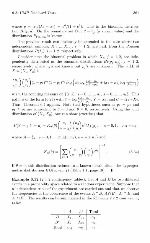
6.2. UMP Unbiased Tests 361
where p = λ2/(λ1 + λ2) = eθ/(1 + eθ). This is the binomial distribu-tion Bi(p, u). On the boundary set Θ01, θ = θj (a known value) and thedistribution PY |U=u is known.
The previous result can obviously be extended to the case where twoindependent samples, Xi1, ..., Xini
, i = 1, 2, are i.i.d. from the Poissondistributions P (λi), i = 1, 2, respectively.
Consider next the binomial problem in which Xj , j = 1, 2, are inde-pendently distributed as the binomial distributions Bi(pj , nj), j = 1, 2,respectively, where nj ’s are known but pj ’s are unknown. The p.d.f. ofX = (X1, X2) is(n1
x1
)(n2
x2
)(1 − p1)n1(1 − p2)n2exp
x2 log p2(1−p1)
p1(1−p2)+ (x1 + x2) log p1
(1−p1)
w.r.t. the counting measure on (i, j) : i = 0, 1, ..., n1, j = 0, 1, ..., n2. Thisp.d.f. is of the form (6.23) with θ = log p2(1−p1)
p1(1−p2), Y = X2, and U = X1+X2.
Thus, Theorem 6.4 applies. Note that hypotheses such as p1 = p2 andp1 ≥ p2 are equivalent to θ = 0 and θ ≤ 0, respectively. Using the jointdistribution of (X1, X2), one can show (exercise) that
P (Y = y|U = u) = Ku(θ)(
n1
u− y
)(n2
y
)eθyIA(y), u = 0, 1, ..., n1 + n2,
where A = y : y = 0, 1, ...,min(u, n2), u− y ≤ n1 and
Ku(θ) =
⎡⎣∑y∈A
(n1
u− y
)(n2
y
)eθy
⎤⎦−1
. (6.34)
If θ = 0, this distribution reduces to a known distribution: the hypergeo-metric distribution HG(u, n2, n1) (Table 1.1, page 18).
Example 6.12 (2 × 2 contingency tables). Let A and B be two differentevents in a probability space related to a random experiment. Suppose thatn independent trials of the experiment are carried out and that we observethe frequencies of the occurrence of the events A∩B, A∩Bc, Ac ∩B, andAc ∩Bc. The results can be summarized in the following 2× 2 contingencytable:
A Ac TotalB X11 X12 n1
Bc X21 X22 n2
Total m1 m2 n
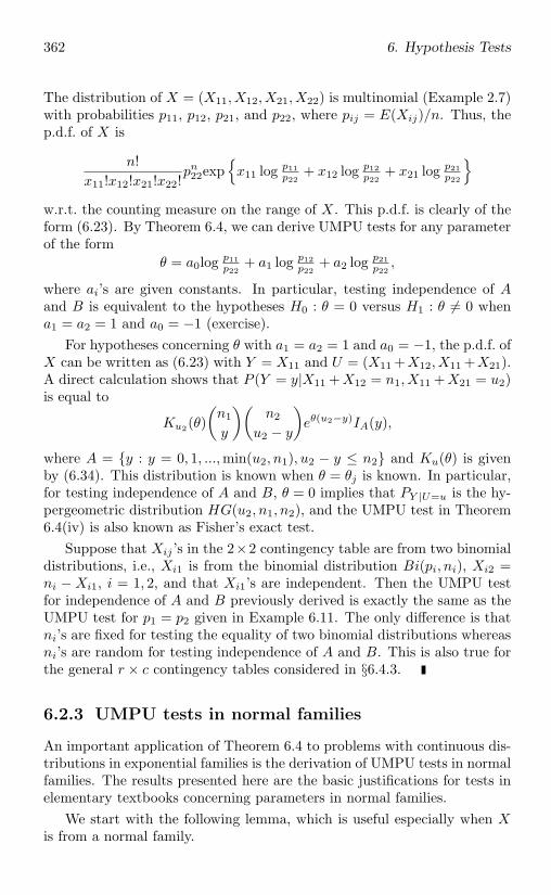
362 6. Hypothesis Tests
The distribution of X = (X11, X12, X21, X22) is multinomial (Example 2.7)with probabilities p11, p12, p21, and p22, where pij = E(Xij)/n. Thus, thep.d.f. of X is
n!x11!x12!x21!x22!
pn22expx11 log p11
p22+ x12 log p12
p22+ x21 log p21
p22
w.r.t. the counting measure on the range of X. This p.d.f. is clearly of theform (6.23). By Theorem 6.4, we can derive UMPU tests for any parameterof the form
θ = a0log p11p22
+ a1 log p12p22
+ a2 log p21p22
,
where ai’s are given constants. In particular, testing independence of Aand B is equivalent to the hypotheses H0 : θ = 0 versus H1 : θ = 0 whena1 = a2 = 1 and a0 = −1 (exercise).
For hypotheses concerning θ with a1 = a2 = 1 and a0 = −1, the p.d.f. ofX can be written as (6.23) with Y = X11 and U = (X11 +X12, X11 +X21).A direct calculation shows that P (Y = y|X11 +X12 = n1, X11 +X21 = u2)is equal to
Ku2(θ)(n1
y
)(n2
u2 − y
)eθ(u2−y)IA(y),
where A = y : y = 0, 1, ...,min(u2, n1), u2 − y ≤ n2 and Ku(θ) is givenby (6.34). This distribution is known when θ = θj is known. In particular,for testing independence of A and B, θ = 0 implies that PY |U=u is the hy-pergeometric distribution HG(u2, n1, n2), and the UMPU test in Theorem6.4(iv) is also known as Fisher’s exact test.
Suppose that Xij ’s in the 2×2 contingency table are from two binomialdistributions, i.e., Xi1 is from the binomial distribution Bi(pi, ni), Xi2 =ni − Xi1, i = 1, 2, and that Xi1’s are independent. Then the UMPU testfor independence of A and B previously derived is exactly the same as theUMPU test for p1 = p2 given in Example 6.11. The only difference is thatni’s are fixed for testing the equality of two binomial distributions whereasni’s are random for testing independence of A and B. This is also true forthe general r × c contingency tables considered in §6.4.3.
6.2.3 UMPU tests in normal families
An important application of Theorem 6.4 to problems with continuous dis-tributions in exponential families is the derivation of UMPU tests in normalfamilies. The results presented here are the basic justifications for tests inelementary textbooks concerning parameters in normal families.
We start with the following lemma, which is useful especially when Xis from a normal family.
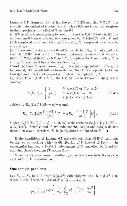
6.2. UMP Unbiased Tests 363
Lemma 6.7. Suppose that X has the p.d.f. (6.23) and that V (Y,U) is astatistic independent of U when θ = θj , where θj ’s are known values givenin the hypotheses in (i)-(iv) of Theorem 6.4.(i) If V (y, u) is increasing in y for each u, then the UMPU tests in (i)-(iii)of Theorem 6.4 are equivalent to those given by (6.24)-(6.28) with Y and(Y,U) replaced by V and with ci(U)’s and γi(U)’s replaced by constantsci’s and γi’s.(ii) If there are functions a(u) > 0 and b(u) such that V (y, u) = a(u)y+b(u),then the UMPU test in (iv) of Theorem 6.4 is equivalent to that given by(6.25), (6.28), and (6.29) with Y and (Y,U) replaced by V and with ci(U)’sand γi(U)’s replaced by constants ci’s and γi’s.Proof. (i) Since V is increasing in y, Y > ci(u) is equivalent to V > di(u)for some di. The result follows from the fact that V is independent of U sothat di’s and γi’s do not depend on u when Y is replaced by V .(ii) Since V = a(U)Y + b(U), the UMPU test in Theorem 6.4(iv) is thesame as
T∗(V,U) =
⎧⎨⎩1 V < c1(U) or V > c2(U)γi(U) V = ci(U), i = 1, 2,0 c1(U) < V < c2(U),
(6.35)
subject to Eθ0 [T∗(V,U)|U = u] = α and
Eθ0
[T∗(V,U)
V − b(U)a(U)
∣∣∣∣U]= αEθ0
[V − b(U)a(U)
∣∣∣∣U]. (6.36)
Under Eθ0 [T∗(V,U)|U = u] = α, (6.36) is the same as Eθ0 [T∗(V,U)V |U ] =αEθ0(V |U). Since V and U are independent, ci(u)’s and γi(u)’s do notdepend on u and, therefore, T∗ in (6.35) does not depend on U .
If the conditions of Lemma 6.7 are satisfied, then UMPU tests canbe derived by working with the distribution of V instead of PY |U=u. Inexponential families, a V (Y,U) independent of U can often be found byapplying Basu’s theorem (Theorem 2.4).
When we consider normal families, γi’s can be chosen to be 0 since thec.d.f. of Y or V is continuous.
One-sample problems
Let X1, ..., Xn be i.i.d. from N(µ, σ2) with unknown µ ∈ R and σ2 > 0,where n ≥ 2. The joint p.d.f. of X = (X1, ..., Xn) is
1(2πσ2)n/2
exp
− 1
2σ2
n∑i=1
x2i +
nµ
σ2 x− nµ2
2σ2
.
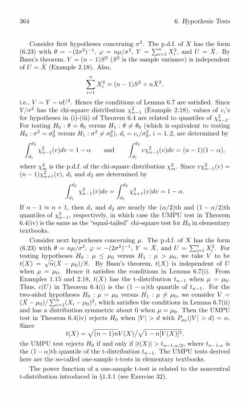
364 6. Hypothesis Tests
Consider first hypotheses concerning σ2. The p.d.f. of X has the form(6.23) with θ = −(2σ2)−1, ϕ = nµ/σ2, Y =
∑ni=1 X
2i , and U = X. By
Basu’s theorem, V = (n− 1)S2 (S2 is the sample variance) is independentof U = X (Example 2.18). Also,
n∑i=1
X2i = (n− 1)S2 + nX2,
i.e., V = Y − nU2. Hence the conditions of Lemma 6.7 are satisfied. SinceV/σ2 has the chi-square distribution χ2
n−1 (Example 2.18), values of ci’sfor hypotheses in (i)-(iii) of Theorem 6.4 are related to quantiles of χ2
n−1.For testing H0 : θ = θ0 versus H1 : θ = θ0 (which is equivalent to testingH0 : σ2 = σ2
0 versus H1 : σ2 = σ20), di = ci/σ
20 , i = 1, 2, are determined by∫ d2
d1
χ2n−1(v)dv = 1 − α and
∫ d2
d1
vχ2n−1(v)dv = (n− 1)(1 − α),
where χ2m is the p.d.f. of the chi-square distribution χ2
m. Since vχ2n−1(v) =
(n− 1)χ2n+1(v), d1 and d2 are determined by∫ d2
d1
χ2n−1(v)dv =
∫ d2
d1
χ2n+1(v)dv = 1 − α.
If n − 1 ≈ n + 1, then d1 and d2 are nearly the (α/2)th and (1 − α/2)thquantiles of χ2
n−1, respectively, in which case the UMPU test in Theorem6.4(iv) is the same as the “equal-tailed” chi-square test for H0 in elementarytextbooks.
Consider next hypotheses concerning µ. The p.d.f. of X has the form(6.23) with θ = nµ/σ2, ϕ = −(2σ2)−1, Y = X, and U =
∑ni=1 X
2i . For
testing hypotheses H0 : µ ≤ µ0 versus H1 : µ > µ0, we take V to bet(X) =
√n(X − µ0)/S. By Basu’s theorem, t(X) is independent of U
when µ = µ0. Hence it satisfies the conditions in Lemma 6.7(i). FromExamples 1.15 and 2.18, t(X) has the t-distribution tn−1 when µ = µ0.Thus, c(U) in Theorem 6.4(i) is the (1 − α)th quantile of tn−1. For thetwo-sided hypotheses H0 : µ = µ0 versus H1 : µ = µ0, we consider V =(X − µ0)/
∑ni=1(Xi − µ0)2, which satisfies the conditions in Lemma 6.7(ii)
and has a distribution symmetric about 0 when µ = µ0. Then the UMPUtest in Theorem 6.4(iv) rejects H0 when |V | > d with Pµ0(|V | > d) = α.Since
t(X) =√
(n− 1)nV (X)/√
1 − n[V (X)]2,
the UMPU test rejects H0 if and only if |t(X)| > tn−1,α/2, where tn−1,α isthe (1− α)th quantile of the t-distribution tn−1. The UMPU tests derivedhere are the so-called one-sample t-tests in elementary textbooks.
The power function of a one-sample t-test is related to the noncentralt-distribution introduced in §1.3.1 (see Exercise 32).
6.2. UMP Unbiased Tests 365
Two-sample problems
The problem of comparing the parameters of two normal distributions arisesin the comparison of two treatments, products, and so on (see also Example6.11). Suppose that we have two independent samples, Xi1, ..., Xini
, i =1, 2, i.i.d. from N(µi, σ
2i ), i = 1, 2, respectively, where ni ≥ 2. The joint
p.d.f. of Xij ’s is
C(µ1, µ2, σ21 , σ
22) exp
⎧⎨⎩−2∑
i=1
12σ2
i
ni∑j=1
x2ij +
2∑i=1
niµi
σ2i
xi
⎫⎬⎭ ,
where xi is the sample mean based on xi1, ..., xini and C(·) is a knownfunction.
Consider first the hypothesis H0 : σ22/σ
21 ≤ ∆0 or H0 : σ2
2/σ21 = ∆0.
The p.d.f. of Xij ’s is of the form (6.23) with
θ =1
2∆0σ21− 1
2σ22, ϕ =
(− 1
2σ21,n1µ1
σ21
,n2µ2
σ22
),
Y =n2∑j=1
X22j , U =
⎛⎝ n1∑j=1
X21j +
1∆0
n2∑j=1
X22j , X1, X2
⎞⎠ .
To apply Lemma 6.7, consider
V =(n2 − 1)S2
2/∆0
(n1 − 1)S21 + (n2 − 1)S2
2/∆0=
(Y − n2U3)/∆0
U1 − n1U2 − n2U3/∆0,
where S2i is the sample variance based on Xi1, ..., Xini
and Uj is the jthcomponent of U . By Basu’s theorem, V and U are independent whenθ = 0 (σ2
2 = ∆0σ21). Since V is increasing and linear in Y , the conditions
of Lemma 6.7 are satisfied. Thus, a UMPU test rejects H0 : θ ≤ 0 (whichis equivalent to H0 : σ2
2/σ21 ≤ ∆0) when V > c0 with Pθ=0(V > c0) = α;
a UMPU test rejects H0 : θ = 0 (which is equivalent to H0 : σ22/σ
21 =
∆0) when V < c1 or V > c2 with Pθ=0(c1 < V < c2) = 1 − α andEθ=0[V T∗(V )] = αEθ=0(V ). Note that
V =(n2 − 1)F
n1 − 1 + (n2 − 1)Fwith F =
S22/∆0
S21
.
It follows from Example 1.15 that F has the F-distribution Fn2−1,n1−1 (Ta-ble 1.2, page 20) when θ = 0. Since V is a strictly increasing function ofF, a UMPU test rejects H0 : θ ≤ 0 when F > Fn2−1,n1−1,α, where Fa,b,α
is the (1 − α)th quantile of the F-distribution Fa,b. This is the F-test inelementary textbooks.
366 6. Hypothesis Tests
When θ = 0, V has the beta distribution B((n2 − 1)/2, (n1 − 1)/2) andEθ=0(V ) = (n2−1)/(n1+n2−2) (Table 1.2). Then condition Eθ=0[V T∗(V )]= αEθ=0(V ) is the same as
(1 − α)(n2 − 1)n1 + n2 − 2
=∫ c2
c1
vf(n2−1)/2,(n1−1)/2(v)dv,
where fa,b is the p.d.f. of the beta distribution B(a, b). Using the fact thatvf(n2−1)/2,(n1−1)/2(v) = (n1 + n2 − 2)−1(n2 − 1)f(n2+1)/2,(n1−1)/2(v), weconclude that a UMPU test rejects H0 : θ = 0 when V < c1 or V > c2,where c1 and c2 are determined by
1 − α =∫ c2
c1
vf(n2−1)/2,(n1−1)/2(v)dv =∫ c2
c1
f(n2+1)/2,(n1−1)/2(v)dv.
If n2 − 1 ≈ n2 + 1 (i.e., n2 is large), then this UMPU test can be ap-proximated by the F-test which rejects H0 : θ = 0 if and only if F <Fn2−1,n1−1,1−α/2 or F > Fn2−1,n1−1,α/2.
Consider next the hypothesis H0 : µ1 ≥ µ2 or H0 : µ1 = µ2. If σ21 = σ2
2 ,the problem is the so-called Behrens-Fisher problem and is not accessible bythe method introduced in this section. We now assume that σ2
1 = σ22 = σ2
but σ2 is unknown. The p.d.f. of Xij ’s is then
C(µ1, µ2, σ2) exp
⎧⎨⎩− 12σ2
2∑i=1
ni∑j=1
x2ij +
n1µ1
σ2 x1 +n2µ2
σ2 x2
⎫⎬⎭ ,
which is of the form (6.23) with
θ =µ2 − µ1
(n−11 + n−1
2 )σ2, ϕ =
(n1µ1 + n2µ2
(n1 + n2)σ2 , − 12σ2
),
Y = X2 − X1, U =
⎛⎝n1X1 + n2X2,
2∑i=1
ni∑j=1
X2ij
⎞⎠ .
For testing H0 : θ ≤ 0 (i.e., µ1 ≥ µ2) versus H1 : θ > 0, we consider V inLemma 6.7 to be
t(X) =(X2 − X1)
/√n−1
1 + n−12√
[(n1 − 1)S21 + (n2 − 1)S2
2 ]/(n1 + n2 − 2). (6.37)
When θ = 0, t(X) is independent of U (Basu’s theorem) and satisfiesthe conditions in Lemma 6.7(i); the numerator and the denominator oft(X) (after division by σ) are independently distributed as N(0, 1) and
6.2. UMP Unbiased Tests 367
the chi-square distribution χ2n1+n2−2, respectively. Hence t(X) has the t-
distribution tn1+n2−2 and a UMPU test rejects H0 when t(X) > tn1+n2−2,α,where tn1+n2−2,α is the (1 − α)th quantile of the t-distribution tn1+n2−2.This is the so-called (one-sided) two-sample t-test.
For testing H0 : θ = 0 (i.e., µ1 = µ2) versus H1 : θ = 0, it follows from asimilar argument used in the derivation of the (two-sided) one-sample t-testthat a UMPU test rejects H0 when |t(X)| > tn1+n2−2,α/2 (exercise). Thisis the (two-sided) two-sample t-test.
The power function of a two-sample t-test is related to a noncentralt-distribution.
Normal linear models
Consider linear model (3.25) with assumption A1, i.e.,
X = (X1, ..., Xn) is Nn(βZτ , σ2In), (6.38)
where β is a p-vector of unknown parameters, Z = (Zτ1 , ..., Z
τn)τ , Zi’s are the
values of a p-vector of deterministic covariates, and σ2 > 0 is an unknownparameter. Assume that n > p and the rank of Z is r ≤ p. Let l ∈ R(Z)(the linear space generated by the rows of Z) and θ0 be a fixed constant.We consider the hypotheses
H0 : βlτ ≤ θ0 versus H1 : βlτ > θ0 (6.39)
orH0 : βlτ = θ0 versus H1 : βlτ = θ0. (6.40)
Since H = Z(ZτZ)−Zτ is a projection matrix of rank r, there exists ann× n orthogonal matrix Γ such that
Γ = (Γ1,Γ2) and HΓ = (Γ1, 0), (6.41)
where Γ1 is n×r and Γ2 is n×(n−r). Let Yj = XΓj , j = 1, 2. Consider thetransformation (Y1, Y2) = XΓ. Since ΓτΓ = In and X is Nn(βZτ , σ2In),(Y1, Y2) is Nn(βZτΓ, σ2In). It follows from (6.41) that
E(Y2) = E(XΓ2) = βZτΓ2 = βZτHΓ2 = 0.
Let η = βZτΓ1 = E(Y1). Then the p.d.f. of (Y1, Y2) is
1(2πσ2)n/2
expY1η
τ
σ2 − ‖Y1‖2 + ‖Y2‖2
2σ2 − ‖η‖2
2σ2
. (6.42)
Since l in (6.39) or (6.40) is in R(Z), there exists λ ∈ Rn such that l = λZ.Then
βlτ = XHλτ = XHΓΓτλτ = XΓ1Γτ1λ
τ = Y1Γτ1λ
τ , (6.43)
368 6. Hypothesis Tests
where β is the LSE defined by (3.27). By (6.43) and Theorem 3.6(ii),
E(βlτ ) = βlτ = E(Y1)Γτ1λ
τ = ηaτ ,
where a = λΓ1. Let η = (η1, ..., ηr) and a = (a1, ..., ar). Without loss ofgenerality, we assume that a1 = 0. Then the p.d.f. in (6.42) is of the form(6.23) with
θ =ηaτ
a1σ2 , ϕ =(− 1
2σ2 ,η2
σ2 , ...,ηrσ2
),
Y = Y11, U =(‖Y1‖2 + ‖Y2‖2, Y12 −
a2Y11
a1, ..., Y1r −
arY11
a1
),
where Y1j is the jth component of Y1. By Basu’s theorem,
t(X) =√n− r(Y1a
τ − θ0)‖Y2‖ ‖a‖
is independent of U when ηaτ = βlτ = θ0. Note that ‖Y2‖2 = SSR in(3.36) and ‖a‖2 = λΓ1Γτ
1λτ = λHλτ = l(ZτZ)−lτ . Hence, by (6.43),
t(X) =βlτ − θ0√
l(ZτZ)−lτ√SSR/(n− r)
,
which has the t-distribution tn−r (Theorem 3.8). Using the same argumentsin deriving the one-sample or two-sample t-test, we obtain that a UMPUtest for the hypotheses in (6.39) rejects H0 when t(X) > tn−r,α, and that aUMPU test for the hypotheses in (6.40) rejects H0 when |t(X)| > tn−r,α/2.
Testing for independence in the bivariate normal family
Suppose that X1, ..., Xn are i.i.d. from a bivariate normal distribution, i.e.,the p.d.f. of X = (X1, ..., Xn) is
1(2πσ1σ2
√1−ρ2)n
exp− ‖Y1−µ1‖2
2σ21(1−ρ2) + ρ(Y1−µ1)(Y2−µ2)τ
σ1σ2(1−ρ2) − ‖Y2−µ2‖2
2σ22(1−ρ2)
, (6.44)
where Yj is the n-vector containing the jth components of X1, ..., Xn, j =1, 2.
Testing for independence of the two components of X1 (or Y1 and Y2) isequivalent to testing H0 : ρ = 0 versus H1 : ρ = 0. In some cases one mayalso be interested in the one-sided hypotheses H0 : ρ ≤ 0 versus H1 : ρ > 0.It can be shown (exercise) that the p.d.f. in (6.44) is of the form (6.23) withθ = ρ
σ1σ2(1−ρ2) and
Y =n∑
i=1
Xi1Xi2, U =
(n∑
i=1
X2i1,
n∑i=1
X2i2,
n∑i=1
Xi1,
n∑i=1
Xi2
),
6.3. UMP Invariant Tests 369
where Xij is the jth component of Xi, j = 1, 2.The hypothesis ρ ≤ 0 is equivalent to θ ≤ 0. The sample correlation
coefficient
R =n∑
i=1
(Xi1 − X1)(Xi2 − X2)/[
n∑i=1
(Xi1 − X1)2n∑
i=1
(Xi2 − X2)2]1/2
,
where Xj is the sample mean of X1j , ..., Xnj , j = 1, 2, is independent of Uwhen ρ = 0 (Basu’s theorem). To apply Lemma 6.7, we consider
V =√n− 2R/
√1 −R2. (6.45)
It can be shown (exercise) that R is linear in Y and that V has the t-distribution tn−2 when ρ = 0. Hence, a UMPU test for H0 : ρ ≤ 0 versusH1 : ρ > 0 rejects H0 when V > tn−2,α and a UMPU test for H0 : ρ = 0versus H1 : ρ = 0 rejects H0 when |V | > tn−2,α/2, where tn−2,α is the(1 − α)th quantile of the t-distribution tn−2.
6.3 UMP Invariant Tests
In the previous section the unbiasedness principle is considered to derive anoptimal test within the class of unbiased tests when a UMP test does notexist. In this section we study the same problem with unbiasedness replacedby invariance under a given group of transformations. The principles ofunbiasedness and invariance often complement each other in that each issuccessful in cases where the other is not.
6.3.1 Invariance and UMPI tests
The invariance principle considered here is similar to that introduced in§2.3.2 (Definition 2.9) and in §4.2, but is more general in the sense that weare not restricted to location-scale families (although most examples in thissection are about location-scale families).
Definition 6.5. Let X be a sample from P ∈ P.(i) A class G of one-to-one transformations of X is called a group if andonly if gi ∈ G implies g1g2 ∈ G and g−1
i ∈ G.(ii) We say that P is invariant under G if and only if g(PX) = Pg(X) is aone-to-one transformation from P onto P for each g ∈ G.(iii) We say that the problem of testing H0 : P ∈ P0 versus H1 : P ∈ P1 isinvariant under G if and only if both P0 and P1 are invariant under G.
370 6. Hypothesis Tests
(iv) In an invariant testing problem, a test T (X) is said to be invariantunder G if and only if
T (g(x)) = T (x) for all x and g. (6.46)
(v) A test of size α is said to be a uniformly most powerful invariant (UMPI)test if and only if it is UMP within the class of level α tests that are invariantunder G.(vi) A statistic M(X) is said to be maximal invariant under G if and onlyif (6.46) holds with T replaced by M and
M(x1) = M(x2) implies x1 = g(x2) for some g ∈ G. (6.47)
The following result indicates that invariance reduces the data X to amaximal invariant statistic M(X) whose distribution may depend only ona functional of P that shrinks P.
Proposition 6.2. Let M(X) be maximal invariant under G.(i) A test T (X) is invariant under G if and only if there is a function h suchthat T (x) = h(M(x)) for all x.(ii) Suppose that there is a functional θ(P ) on P satisfying θ(g(P )) = θ(P )for all g ∈ G and P ∈ P and
θ(P1) = θ(P2) implies P1 = g(P2) for some g ∈ G
(i.e., θ(P ) is “maximal invariant”). Then the distribution of M(X) dependsonly on θ(P ).Proof. (i) If T (x) = h(M(x)) for all x, then T (g(x)) = h(M(g(x))) =h(M(x)) = T (x) so that T is invariant. If T is invariant and if M(x1) =M(x2), then x1 = g(x2) for some g and T (x1) = T (g(x2)) = T (x2). HenceT is a function of M .(ii) Suppose that θ(P1) = θ(P2). Then P2 = g(P1) for some g ∈ G and forany event B in the range of M(X),
P2(M(X) ∈ B
)= g(P1)
(M(X) ∈ B
)= P1
(M(g(X)) ∈ B
)= P1
(M(X) ∈ B
).
Hence the distribution of M(X) depends only on θ(P ).
In applications, maximal invariants M(X) and θ = θ(P ) are frequentlyreal-valued. If the hypotheses of interest can be expressed in terms of θ, thenthere may exist a test UMP among those depending only on M(X) (e.g.,when the distribution of M(X) is in a parametric family having monotonelikelihood ratio). Such a test is then a UMPI test.
6.3. UMP Invariant Tests 371
Example 6.13 (Location-scale families). Suppose that X has the Lebesguep.d.f. fi,µ(x) = fi(x1 − µ, ..., xn − µ), where n ≥ 2, µ ∈ R is unknown, andfi, i = 0, 1, are known Lebesgue p.d.f.’s. We consider the problem of testing
H0 : X is from f0,µ versus H1 : X is from f1,µ. (6.48)
Consider G = gc : c ∈ R with gc(x) = (x1 + c, ..., xn + c). For any gc ∈ G,it induces a transformation gc(fi,µ) = fi,µ+c and the problem of testing H0versus H1 in (6.48) is invariant under G.
We now show that a maximal invariant under G is D(X)=(D1, ..., Dn−1)= (X1 −Xn, ..., Xn−1 −Xn). First, it is easy to see that D(X) is invariantunder G. Let x = (x1, ..., xn) and y = (y1, ..., yn) be two points in therange of X. Suppose that xi − xn = yi − yn for i = 1, ..., n − 1. Puttingc = yn−xn, we have yi = xi+c for all i. Hence, D(X) is maximal invariantunder G.
By Proposition 1.8, D has the p.d.f.∫fi(d1 + t, ..., dn−1 + t, t)dt under
Hi, i = 0, 1, which does not depend on µ. In fact, in this case Proposition6.2 applies with M(X) = D(X) and θ(fi,µ) = i. If we consider tests thatare functions of D(X), then the problem of testing the hypotheses in (6.48)becomes one of testing a simple hypothesis versus a simple hypothesis. ByTheorem 6.1, the test UMP among functions of D(X), which is then theUMPI test, rejects H0 in (6.48) when∫
f1(d1 + t, ..., dn−1 + t, t)dt∫f0(d1 + t, ..., dn−1 + t, t)dt
=∫f1(x1 + t, ..., xn + t)dt∫f0(x1 + t, ..., xn + t)dt
> c,
where c is determined by the size of the UMPI test.The previous result can be extended to the case of a location-scale family
where the p.d.f. of X is one of fi,µ,σ = 1σn fi
(x1−µ
σ , ..., xn−µσ
), i = 0, 1,
fi,µ,σ is symmetric about µ, the hypotheses of interest are given by (6.48)with fi,µ replaced by fi,µ,σ, and G = gc,r : c ∈ R, r = 0 with gc,r(x) =(rx1+c, ..., rxn+c). When n ≥ 3, it can be shown that a maximal invariantunder G is W (X) = (W1, ...,Wn−2), where Wi = (Xi −Xn)/(Xn−1 −Xn),and that the p.d.f. of W does not depend on (µ, σ). A UMPI test can thenbe derived (exercise).
The next example considers finding a maximal invariant in a problemthat is not a location-scale family problem.
Example 6.14. Let G be the set of n! permutations of the components ofx ∈ Rn. Then a maximal invariant is the vector of order statistics. This isbecause a permutation of the components of x does not change the valuesof these components and two x’s with the same set of ordered componentscan be obtained from each other through a permutation of coordinates.
372 6. Hypothesis Tests
Suppose that P contains continuous c.d.f.’s on Rn. Let G be the classof all transformations of the form g(x) = (ψ(x1), ..., ψ(xn)), where ψ is con-tinuous and strictly increasing. For x = (x1, ..., xn), let R(x) = (R1, ..., Rn)be the vector of ranks (§5.2.2), i.e., xi = x(Ri), where x(j) is the jth or-dered value of xi’s. Clearly, R(g(x)) = R(x) for any g ∈ G. For any xand y in Rn with R(x) = R(y), define ψ(t) = t + (y(1) − x(1)) for t ≤ x(1),ψ(t) = t + (y(n) − x(n)) for t ≥ x(n), and to be linear between x(j) andx(j+1), j = 1, ..., n − 1. Then ψ(xi) = ψ(yi), i = 1, ..., n. This shows thatthe vector of rank statistics is maximal invariant.
When there is a sufficient statistic U(X), it is convenient first to reducethe data to U(X) before applying invariance. If there is a test T (U) UMPamong all invariant tests depending only on U , one would like to concludethat T (U) is a UMPI test. Unfortunately, this may not be true in general,since it is not clear that for any invariant test based on X there is anequivalent invariant test based only on U(X). The following result providesa sufficient condition under which it is enough to consider invariant testsdepending only on U(X). Its proof is omitted and can be found in Lehmann(1986, pp. 297-302).
Proposition 6.3. Let G be a group of transformations on X (the range ofX) and (G,BG , λ) be a measure space with a σ-finite λ. Suppose that thetesting problem under consideration is invariant under G, that for any setA ∈ BX, the set of points (x, g) for which g(x) ∈ A is in σ(BX × BG), andthat λ(B) = 0 implies λ(h g : h ∈ B) = 0 for all g ∈ G. Suppose furtherthat there is a statistic U(X) sufficient for P ∈ P and that U(x1) = U(x2)implies U(g(x1)) = U(g(x2)) for all g ∈ G so that G induces a group GU oftransformations on the range of U through gU (U(x)) = U(g(x)). Then, forany test T (X) invariant under G, there exists a test based on U(X) that isinvariant under G (and GU ) and has the same power function as T (X).
In many problems g(x) = ψ(x, g), where g ranges over a set G in Rm
and ψ is a Borel function on Rn+m. Then the measurability condition inProposition 6.3 is satisfied by choosing BG to be the Borel σ-field on G.In such cases it is usually not difficult to find a measure λ satisfying thecondition in Proposition 6.3.
Example 6.15. Let X1, ..., Xn be i.i.d. from N(µ, σ2) with unknown µ ∈ Rand σ2 > 0. The problem of testing H0 : σ2 ≥ σ2
0 versus H1 : σ2 < σ20
is invariant under G = gc : c ∈ R with gc(x) = (x1 + c, ..., xn + c). Itcan be shown (exercise) that G and the sufficient statistic U = (X, S2)satisfy the conditions in Proposition 6.3 with GU = hc : c ∈ R andhc(u1, u2) = (u1 + c, u2). A maximal invariant under GU is S2. It followsfrom Proposition 6.3, Corollary 6.1, and the fact that (n − 1)S2/σ2
0 has
6.3. UMP Invariant Tests 373
the chi-square distribution χ2n−1 when σ2 = σ2
0 that a UMPI test of size αrejects H0 when (n − 1)S2/σ2
0 ≤ χ2n−1,1−α, where χ2
n−1,α is the (1 − α)thquantile of the chi-square distribution χ2
n−1. This test coincides with theUMPU test given in §6.2.3.
Example 6.16. Let Xi1, ..., Xini , i = 1, 2, be two independent samplesi.i.d. from N(µi, σ
2i ), i = 1, 2, respectively. The problem of testing H0 :
σ22/σ
21 ≤ ∆0 versus H1 : σ2
2/σ21 > ∆0 is invariant under
G = gc1,c2,r : ci ∈ R, i = 1, 2, r > 0
with
gc1,c2,r(x1, x2) = (rx11 + c1, ..., rx1n1 + c1, rx21 + c2, ..., rx2n2 + c2).
It can be shown (exercise) that the sufficient statistic U = (X1, X2, S1, S2)and G satisfy the conditions in Proposition 6.3 with
GU = hc1,c2,r : ci ∈ R, i = 1, 2, r > 0
andhc1,c2,r(u1, u2, u3, u4) = (ru1 + c1, ru2 + c2, ru3, ru4).
A maximal invariant under GU is S2/S1. Let ∆ = σ22/σ
21 . Then (S2
2/S21)/∆
has an F-distribution and, therefore, V = S22/S
21 has a Lebesgue p.d.f. of
the form
f∆(v) = C(∆)v(n2−3)/2[∆ + (n2 − 1)v/(n1 − 1)]−(n1+n2−2)/2I(0,∞)(v),
where C(∆) is a known function of ∆. It can be shown (exercise) that thefamily f∆ : ∆ > 0 has monotone likelihood ratio in V so that a UMPI testof size α rejects H0 when V > Fn2−1,n1−1,α, where Fa,b,α is the (1 − α)thquantile of the F-distribution Fa,b. Again, this UMPI test coincides withthe UMPU test given in §6.2.3.
The following result shows that in Examples 6.15 and 6.16, the fact thatUMPI tests are the same as the UMPU tests is not a simple coincidence.
Proposition 6.4. Consider a testing problem invariant under G. If thereexists a UMPI test of size α, then it is unbiased. If there also exists aUMPU test of size α that is invariant under G, then the two tests have thesame power function on P ∈ P1. If either the UMPI test or the UMPU testis unique a.s. P, then the two tests are equal a.s. P.Proof. We only need to prove that a UMPI test of size α is unbiased. Thisfollows from the fact that the test T ≡ α is invariant under G.
374 6. Hypothesis Tests
The next example shows an application of invariance in a situationwhere a UMPU test may not exist.
Example 6.17. Let X1, ..., Xn be i.i.d. from N(µ, σ2) with unknown µand σ2. Let θ = (µ − u)/σ, where u is a known constant. Consider theproblem of testing H0 : θ ≤ θ0 versus H1 : θ > θ0. Note that H0 is thesame as P (X1 ≤ u) ≥ p0 for a known constant p0 = Φ(−θ0). Without lossof generality, we consider the case of u = 0.
The problem is invariant under G = gr : r > 0 with gr(x) = rx. ByProposition 6.3, we can consider tests that are functions of the sufficientstatistic (X, S2) only. A maximal invariant under G is t(X) =
√nX/S. To
find a UMPI test, it remains to find a test UMP among all tests that arefunctions of t(X).
From the discussion in §1.3.1, t(X) has the noncentral t-distributiontn−1(
√nθ). Let fθ(t) be the Lebesgue p.d.f. of t(X), i.e., fθ is given by
(1.32) with n replaced by n − 1 and δ =√nθ. It can be shown (exercise)
that the family of p.d.f.’s, fθ(t) : θ ∈ R, has monotone likelihood ratio int. Hence, by Theorem 6.2, a UMPI test of size α rejects H0 when t(X) > c,where c is the (1 − α)th quantile of tn−1(
√nθ0).
In some problems we may have to apply both unbiasedness and invari-ance principles. For instance, suppose that in the current problem we wouldlike to test H0 : θ = θ0 versus H1 : θ = θ0. The problem is still invariantunder G. Following the previous discussion, we only need to consider teststhat are functions of t(X). But a test UMP among functions of t(X) doesnot exist in this case. A test UMP among all unbiased tests that are func-tions of t(X) rejects H0 when t(X) < c1 or t(X) > c2, where c1 and c2 aredetermined by∫ c2
c1
fθ0(t)dt = 1 − α andd
dθ
[∫ c2
c1
fθ(t)dt] ∣∣∣∣
θ=θ0
= 0
(see Exercise 24). This test is then UMP among all tests that are unbiasedand invariant. Whether it is also UMPU without the restriction to invarianttests is an open problem.
6.3.2 UMPI tests in normal linear models
Consider normal linear model (6.38):
X = Nn(βZτ , σ2In),
where β is a p-vector of unknown parameters, σ2 > 0 is unknown, and Z isa fixed n× p matrix of rank r ≤ p < n. In §6.2.3, UMPU tests for testing
6.3. UMP Invariant Tests 375
(6.39) or (6.40) are derived. A frequently encountered problem in practiceis to test
H0 : βLτ = 0 versus H1 : βLτ = 0, (6.49)
where L is an s × p matrix of rank s ≤ r and all rows of L are in R(Z).However, a UMPU test for (6.49) does not exist if s > 1. We now derivea UMPI test for testing (6.49). We use without proof the following resultfrom linear algebra: there exists an orthogonal matrix Γ such that
(η, 0) = βZτΓ,
where η is an r-vector and 0 is the (n− r)-vector of 0’s, and that (6.49) isequivalent to
H0 : η1 = 0 versus H1 : η1 = 0, (6.50)
where η1 is the s-vector containing the first s components of η. Let Y =(Y1, Y2) = XΓ, where Y1 is r×1. Then Y = Nn((η, 0), σ2In) with the p.d.f.given by (6.42). Let Y1 = (Y11, Y12), where Y11 is s× 1, and let
G = gΛ,c,γ : c ∈ Rr−s, γ > 0, Λ is an s× s orthogonal matrix
withgΛ,c,γ(Y ) = γ(Y11Λ, Y12 + c, Y2).
Testing (6.50) is invariant under G. By Proposition 6.3, we can restrict ourattention to the sufficient statistic (Y1, ‖Y2‖2). The statistic
M(Y ) = ‖Y11‖2/‖Y2‖2 (6.51)
is clearly invariant. We now show that M(Y ) is maximal invariant. Letui ∈ Rs, ui = 0, and ti ∈ (0,∞), i = 1, 2. If ‖u1‖2/t21 = ‖u2‖2/t22,then t1 = γt2 with γ = ‖u1‖/‖u2‖. Since u1/‖u1‖ and u2/‖u2‖ are twopoints having the same distance from the origin, there exists an orthogonalmatrix Λ such that u1/‖u1‖ = (u2/‖u2‖)Λ, i.e., u1 = γu2Λ. This provesthat if M(y(1)) = M(y(2)) for two points y(1) and y(2) in Rn, then y
(1)11 =
γy(2)11 Λ and ‖y(1)
2 ‖ = γ‖y(2)2 ‖ for some γ > 0 and orthogonal matrix Λ
and, therefore, y(1) = gΛ,c,γ(y(2)) with c = γ−1y(1)12 − y
(2)12 . Thus, M(Y ) is
maximal invariant under G.It can be shown (exercise) that W = M(Y )(n− r)/s has the noncentral
F-distribution Fs,n−r(θ) with θ = ‖η1‖2/σ2 (see §1.3.1). Let fθ(w) be theLebesgue p.d.f. of W , i.e., fθ is given by (1.33) with n1 = s, n2 = n − r,and δ = θ. Note that under H0, θ = 0 and fθ reduces to the p.d.f. of thecentral F-distribution Fs,n−r (Table 1.2, page 20). Also, it can be shown(exercise) that the ratio fθ1(w)/f0(w) is an increasing function of w for anygiven θ1 = 0. By Theorem 6.1, a UMPI test of size α for testing H0 : θ = 0versus H1 : θ = θ1 rejects H0 when W > Fs,n−r,α, where Fs,n−r,α is the
376 6. Hypothesis Tests
(1 − α)th quantile of the F-distribution Fs,n−r. Since this test does notdepend on θ1, by Lemma 6.1, it is also a UMPI test of size α for testingH0 : θ = 0 versus H1 : θ = 0, which is equivalent to testing (6.50).
In applications it is not convenient to carry out the test by findingexplicitly the orthogonal matrix Γ. Hence, we now express the statistic Win terms of X. Since Y = XΓ and E(Y ) = E(X)Γ = βZτΓ,
‖Y1 − η‖2 + ‖Y2‖2 = ‖X − βZτ‖2
and, therefore,
minη
‖Y1 − η‖2 + ‖Y2‖2 = minβ
‖X − βZτ‖2,
which is the same as
‖Y2‖2 = ‖X − βZτ‖2 = SSR,
where β is the LSE defined by (3.27). Similarly,
‖Y11‖2 + ‖Y2‖2 = minβ:βLτ=0
‖X − βZτ‖2.
If we define βH0 to be a solution of
‖X − βH0Zτ‖2 = min
β:βLτ=0‖X − βZτ‖2,
which is called the LSE of β under H0 or the LSE of β subject to βLτ = 0,then
W =(‖X − βH0Z
τ‖2 − ‖X − βZτ‖2)/s
‖X − βZτ‖2/(n− r). (6.52)
Thus, the UMPI test for (6.49) can be used without finding Γ.When s = 1, the UMPI test derived here is the same as the UMPU test
for (6.40) given in §6.2.3.
Example 6.18. Consider the one-way ANOVA model in Example 3.13:
Xij = N(µi, σ2), j = 1, ..., ni, i = 1, ...,m,
and Xij ’s are independent. A common testing problem in applications isthe test for homogeneity of means, i.e.,
H0 : µ1 = · · · = µm versus H1 : µi = µk for some i = k. (6.53)
One can easily find a matrix L for which (6.53) is equivalent to (6.49).But it is not necessary to find such a matrix in order to compute the
6.3. UMP Invariant Tests 377
statistic W that defines the UMPI test. Note that the LSE of (µ1, ..., µm)is (X1·, ..., Xm·), where Xi· is the sample mean based on Xi1, ..., Xini
, andthe LSE under H0 is simply X, the sample mean based on all Xij ’s. Thus,
SSR = ‖X − βZτ‖2 =m∑i=1
ni∑j=1
(Xij − Xi·)2,
SST = ‖X − βH0Zτ‖2 =
m∑i=1
ni∑j=1
(Xij − X)2,
and
SSA = SST − SSR =m∑i=1
ni(Xi· − X)2.
Then
W =SSA/(m− 1)SSR/(n−m)
,
where n =∑m
i=1 ni. The name ANOVA comes from the fact that the UMPItest is carried out by comparing two sources of variation: the variationwithin each group of observations (measured by SSR) and the variationamong m groups (measured by SSA), and that SSA+ SSR = SST is thetotal variation in the data set.
In this case, the distribution of W can also be derived using Cochran’stheorem (Theorem 1.5). See Exercise 64.
Example 6.19. Consider the two-way balanced ANOVA model in Exam-ple 3.14:
Xijk = N(µij , σ2), i = 1, ..., a, j = 1, ..., b, k = 1, ..., c,
where µij = µ+αi+βj+γij ,∑a
i=1 αi =∑b
j=1 βj =∑a
i=1 γij =∑b
j=1 γij =0, and Xijk’s are independent. Typically the following hypotheses are ofinterest:
H0 : αi = 0 for all i versus H1 : αi = 0 for some i, (6.54)
H0 : βj = 0 for all j versus H1 : βj = 0 for some j, (6.55)
and
H0 : γij = 0 for all i, j versus H1 : γij = 0 for some i, j. (6.56)
In applications, αi’s are effects of a factor A (a variable taking finitely manyvalues), βj ’s are effects of a factor B, and γij ’s are effects of the interactionof factors A and B. Hence, testing hypotheses in (6.54), (6.55), and (6.56)
378 6. Hypothesis Tests
are the same as testing effects of factor A, of factor B, and of the interactionbetween A and B, respectively.
The LSE of µ, αi, βj , and γij are given by (Example 3.14) µ = X···,αi = Xi·· − X···, βj = X·j· − X···, γij = Xij· − Xi·· − X·j· + X···, and a dotis used to denote averaging over the indicated subscript. Let
SSR =a∑
i=1
b∑j=1
c∑k=1
(Xijk − Xij·)2,
SSA = bca∑
i=1
(Xi·· − X···)2,
SSB = ac
b∑j=1
(X·j· − X···)2,
and
SSC = c
a∑i=1
b∑j=1
(Xij· −Xi·· −X·j· + X···)2.
Then, one can show (exercise) that for testing (6.54), (6.55), and (6.56),the statistics W in (6.52) (for the UMPI tests) are, respectively,
SSA/(a− 1)SSR/[(c− 1)ab]
,SSB/(b− 1)
SSR/[(c− 1)ab], and
SSC/[(a− 1)(b− 1)]SSR/[(c− 1)ab]
.
We end this section with a discussion of testing for random effects inthe following balanced one-way random effects model (Example 3.17):
Xij = µ + Ai + eij , i = 1, ..., a, j = 1, ..., b, (6.57)
where µ is an unknown parameter, Ai’s are i.i.d. random effects fromN(0, σ2
a), eij ’s are i.i.d. measurement errors from N(0, σ2), and Ai’s andeij ’s are independent. Consider the problem of testing
H0 : σ2a/σ
2 ≤ ∆0 versus H1 : σ2a/σ
2 > ∆0 (6.58)
for a given ∆0. When ∆0 is small, hypothesis H0 in (6.58) means that therandom effects are negligible relative to the measurement variation.
Let (Yi1, ..., Yib) = (Xi1, ..., Xib)Γ, where Γ is a b× b orthogonal matrixwhose elements in the first column are all equal to 1/
√b. Then
Yi1 =√bXi· =
√b(µ + Ai + ei·), i = 1, ..., a,
6.3. UMP Invariant Tests 379
are i.i.d. from N(√bµ, σ2 + bσ2
a), Yij , i = 1, ..., a, j = 2, ..., b, are i.i.d. fromN(0, σ2), and Yij ’s are independent. The reason why E(Yij) = 0 whenj > 1 is because column j of Γ is orthogonal to the first column of Γ.
Let Λ be an a×a orthogonal matrix whose elements in the first columnare all equal to 1/
√a and (U11, ..., Ua1) = (Y1·, ..., Ya·)Λ. Then U11 =
√aY·1
is N(√abµ, σ2 + bσ2
a), Ui1, i = 2, ..., a, are from N(0, σ2 + bσ2a), and Ui1’s
are independent. Let Uij = Yij for j = 2, ..., b, i = 1, ..., a.The problem of testing (6.58) is invariant under the group of transfor-
mations that transform U11 to rU11+c and Uij to rUij , (i, j) = (1, 1), wherer > 0 and c ∈ R. It can be shown (exercise) that the maximal invariantunder this group of transformations is SSA/SSR, where
SSA =a∑
i=2
U2i1 and SSR =
a∑i=1
b∑j=2
U2ij .
Note that H0 in (6.58) is equivalent to (σ2 + bσ2a)/σ
2 ≤ 1 + b∆0. Also,SSA/(σ2 + bσ2
a) has the chi-square distribution χ2a−1 and SSR/σ2 has the
chi-square distribution χ2a(b−1). Hence, the p.d.f. of the statistic
W =1
1 + b∆0
SSA/(a− 1)SSR/[a(b− 1)]
is in a family indexed by (σ2 + bσ2a)/σ
2 with monotone likelihood ratioin W . Thus, a UMPI test of size α for testing (6.58) rejects H0 whenW > Fa−1,a(b−1),α, where Fa−1,a(b−1),α is the (1 − α)th quantile of theF-distribution Fa−1,a(b−1).
It remains to express W in terms of Xij ’s. Note that
SSR =a∑
i=1
b∑j=2
Y 2ij =
a∑i=1
⎛⎝ b∑j=1
e2ij − be2
i·
⎞⎠ =a∑
i=1
b∑j=1
(Xij − Xi·)2
and
SSA =a∑
i=1
U2i1 − U2
11 =a∑
i=1
Y 2i1 − aY 2
·1 = b
a∑i=1
(Xi· − X··)2.
The SSR and SSA derived here are the same as those in Example 6.18when ni = b for all i and m = a. It can also be seen that if ∆0 = 0,then testing (6.58) is equivalent to testing H0 : σ2
a = 0 versus H1 : σ2a = 0
and the derived UMPI test is exactly the same as that in Example 6.18,although the testing problems are different in these two cases.
Extensions to balanced two-way random effects models can be found inLehmann (1986, §7.12).
380 6. Hypothesis Tests
6.4 Tests in Parametric Models
A UMP, UMPU, or UMPI test often does not exist in a particular problem.In the rest of this chapter we study some methods for constructing tests thathave intuitive appeal and frequently coincide with optimal tests (UMP orUMPU tests) when optimal tests do exist. We consider tests in parametricmodels in this section, whereas tests in nonparametric models are studiedin §6.5.
When the hypothesis H0 is not simple, it is often difficult or even im-possible to obtain a test that has exactly a given size α, since this involvesfinding a population P that maximizes the power function of the test overall P ∈ P0. In such cases a common approach is to find tests having asymp-totic significance level α (Definition 2.13). This involves finding the limitof the power of a test at P ∈ P0, which is studied in this section and §6.5.
Throughout this section we assume that a sample X is from P ∈ P =fθ : θ ∈ Θ, where fθ’s are p.d.f.’s w.r.t. a common σ-finite measure andΘ ⊂ Rk, and that the testing problem is
H0 : θ ∈ Θ0 versus H1 : θ ∈ Θ1, (6.59)
where Θ0 ∪ Θ1 = Θ and Θ0 ∩ Θ1 = ∅.
6.4.1 Likelihood ratio tests
When both H0 and H1 are simple (i.e., both Θ0 = θ0 and Θ1 = θ1 aresingle-point sets), Theorem 6.1 applies and a UMP test rejects H0 when
fθ1(X)fθ0(X)
> c0 (6.60)
for some c0 > 0, which is equivalent to (exercise)
fθ0(X)max[fθ0(X), fθ1(X)]
< c (6.61)
for some c > 0. The following definition is a natural extension of this idea.
Definition 6.6. Let (θ) = fθ(X) be the likelihood function. For testing(6.59), a likelihood ratio (LR) test is any test that rejects H0 if and only ifλ(X) < c, where c ∈ [0, 1] and λ(X) is the likelihood ratio defined by
λ(X) =supθ∈Θ0
(θ)
supθ∈Θ
(θ).
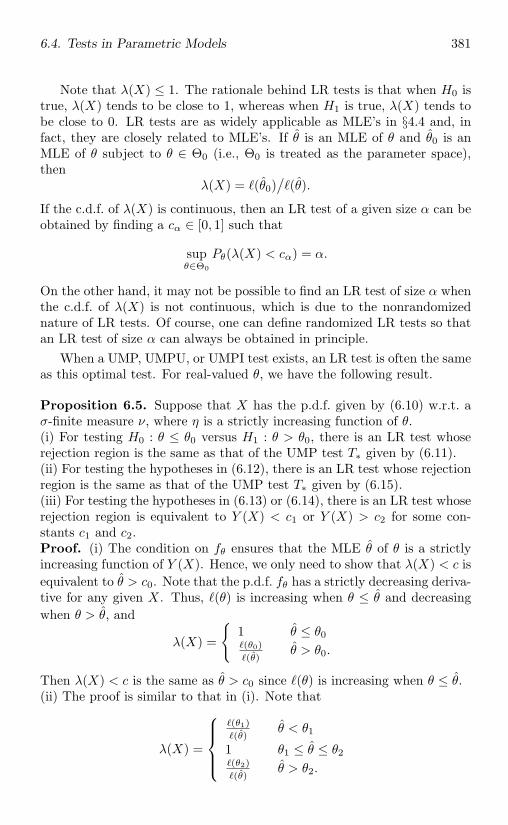
6.4. Tests in Parametric Models 381
Note that λ(X) ≤ 1. The rationale behind LR tests is that when H0 istrue, λ(X) tends to be close to 1, whereas when H1 is true, λ(X) tends tobe close to 0. LR tests are as widely applicable as MLE’s in §4.4 and, infact, they are closely related to MLE’s. If θ is an MLE of θ and θ0 is anMLE of θ subject to θ ∈ Θ0 (i.e., Θ0 is treated as the parameter space),then
λ(X) = (θ0)/(θ).
If the c.d.f. of λ(X) is continuous, then an LR test of a given size α can beobtained by finding a cα ∈ [0, 1] such that
supθ∈Θ0
Pθ(λ(X) < cα) = α.
On the other hand, it may not be possible to find an LR test of size α whenthe c.d.f. of λ(X) is not continuous, which is due to the nonrandomizednature of LR tests. Of course, one can define randomized LR tests so thatan LR test of size α can always be obtained in principle.
When a UMP, UMPU, or UMPI test exists, an LR test is often the sameas this optimal test. For real-valued θ, we have the following result.
Proposition 6.5. Suppose that X has the p.d.f. given by (6.10) w.r.t. aσ-finite measure ν, where η is a strictly increasing function of θ.(i) For testing H0 : θ ≤ θ0 versus H1 : θ > θ0, there is an LR test whoserejection region is the same as that of the UMP test T∗ given by (6.11).(ii) For testing the hypotheses in (6.12), there is an LR test whose rejectionregion is the same as that of the UMP test T∗ given by (6.15).(iii) For testing the hypotheses in (6.13) or (6.14), there is an LR test whoserejection region is equivalent to Y (X) < c1 or Y (X) > c2 for some con-stants c1 and c2.Proof. (i) The condition on fθ ensures that the MLE θ of θ is a strictlyincreasing function of Y (X). Hence, we only need to show that λ(X) < c isequivalent to θ > c0. Note that the p.d.f. fθ has a strictly decreasing deriva-tive for any given X. Thus, (θ) is increasing when θ ≤ θ and decreasingwhen θ > θ, and
λ(X) =
1 θ ≤ θ0(θ0)(θ)
θ > θ0.
Then λ(X) < c is the same as θ > c0 since (θ) is increasing when θ ≤ θ.(ii) The proof is similar to that in (i). Note that
λ(X) =
⎧⎪⎪⎨⎪⎪⎩(θ1)(θ)
θ < θ1
1 θ1 ≤ θ ≤ θ2(θ2)(θ)
θ > θ2.
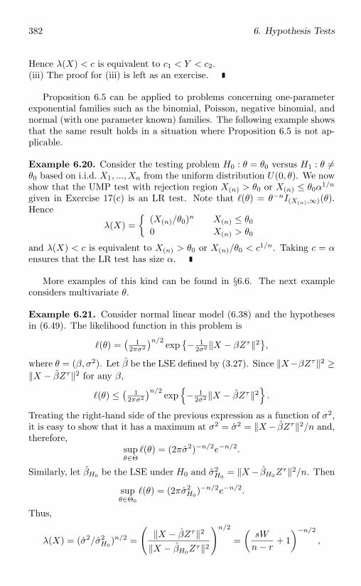
382 6. Hypothesis Tests
Hence λ(X) < c is equivalent to c1 < Y < c2.(iii) The proof for (iii) is left as an exercise.
Proposition 6.5 can be applied to problems concerning one-parameterexponential families such as the binomial, Poisson, negative binomial, andnormal (with one parameter known) families. The following example showsthat the same result holds in a situation where Proposition 6.5 is not ap-plicable.
Example 6.20. Consider the testing problem H0 : θ = θ0 versus H1 : θ =θ0 based on i.i.d. X1, ..., Xn from the uniform distribution U(0, θ). We nowshow that the UMP test with rejection region X(n) > θ0 or X(n) ≤ θ0α
1/n
given in Exercise 17(c) is an LR test. Note that (θ) = θ−nI(X(n),∞)(θ).Hence
λ(X) =
(X(n)/θ0)n X(n) ≤ θ0
0 X(n) > θ0
and λ(X) < c is equivalent to X(n) > θ0 or X(n)/θ0 < c1/n. Taking c = αensures that the LR test has size α.
More examples of this kind can be found in §6.6. The next exampleconsiders multivariate θ.
Example 6.21. Consider normal linear model (6.38) and the hypothesesin (6.49). The likelihood function in this problem is
(θ) =( 1
2πσ2
)n/2 exp− 1
2σ2 ‖X − βZτ‖2,
where θ = (β, σ2). Let β be the LSE defined by (3.27). Since ‖X−βZτ‖2 ≥‖X − βZτ‖2 for any β,
(θ) ≤( 1
2πσ2
)n/2 exp− 1
2σ2 ‖X − βZτ‖2.
Treating the right-hand side of the previous expression as a function of σ2,it is easy to show that it has a maximum at σ2 = σ2 = ‖X− βZτ‖2/n and,therefore,
supθ∈Θ
(θ) = (2πσ2)−n/2e−n/2.
Similarly, let βH0 be the LSE under H0 and σ2H0
= ‖X− βH0Zτ‖2/n. Then
supθ∈Θ0
(θ) = (2πσ2H0
)−n/2e−n/2.
Thus,
λ(X) = (σ2/σ2H0
)n/2 =
(‖X − βZτ‖2
‖X − βH0Zτ‖2
)n/2
=(
sW
n− r+ 1
)−n/2
,
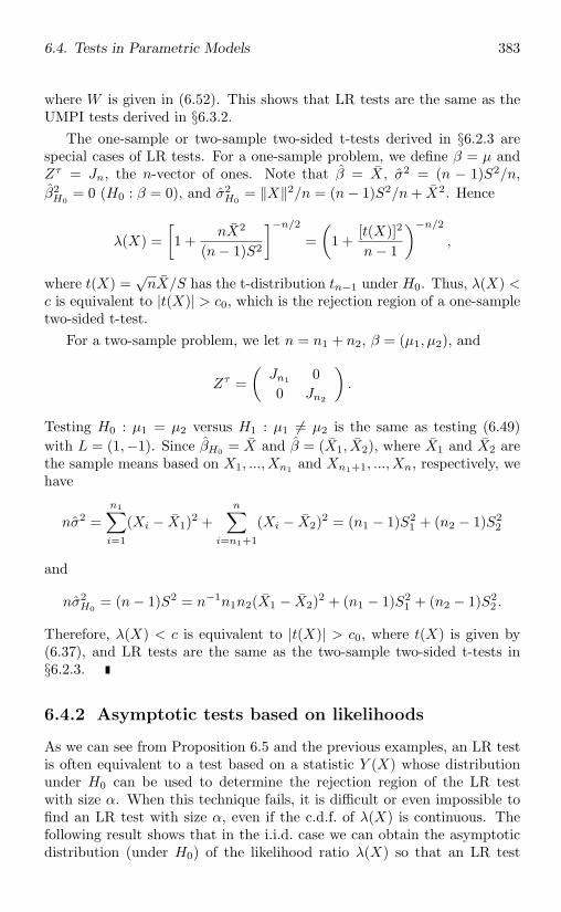
6.4. Tests in Parametric Models 383
where W is given in (6.52). This shows that LR tests are the same as theUMPI tests derived in §6.3.2.
The one-sample or two-sample two-sided t-tests derived in §6.2.3 arespecial cases of LR tests. For a one-sample problem, we define β = µ andZτ = Jn, the n-vector of ones. Note that β = X, σ2 = (n − 1)S2/n,β2H0
= 0 (H0 : β = 0), and σ2H0
= ‖X‖2/n = (n− 1)S2/n + X2. Hence
λ(X) =[1 +
nX2
(n− 1)S2
]−n/2
=(
1 +[t(X)]2
n− 1
)−n/2
,
where t(X) =√nX/S has the t-distribution tn−1 under H0. Thus, λ(X) <
c is equivalent to |t(X)| > c0, which is the rejection region of a one-sampletwo-sided t-test.
For a two-sample problem, we let n = n1 + n2, β = (µ1, µ2), and
Zτ =(
Jn1 00 Jn2
).
Testing H0 : µ1 = µ2 versus H1 : µ1 = µ2 is the same as testing (6.49)with L = (1,−1). Since βH0 = X and β = (X1, X2), where X1 and X2 arethe sample means based on X1, ..., Xn1 and Xn1+1, ..., Xn, respectively, wehave
nσ2 =n1∑i=1
(Xi − X1)2 +n∑
i=n1+1
(Xi − X2)2 = (n1 − 1)S21 + (n2 − 1)S2
2
and
nσ2H0
= (n− 1)S2 = n−1n1n2(X1 − X2)2 + (n1 − 1)S21 + (n2 − 1)S2
2 .
Therefore, λ(X) < c is equivalent to |t(X)| > c0, where t(X) is given by(6.37), and LR tests are the same as the two-sample two-sided t-tests in§6.2.3.
6.4.2 Asymptotic tests based on likelihoods
As we can see from Proposition 6.5 and the previous examples, an LR testis often equivalent to a test based on a statistic Y (X) whose distributionunder H0 can be used to determine the rejection region of the LR testwith size α. When this technique fails, it is difficult or even impossible tofind an LR test with size α, even if the c.d.f. of λ(X) is continuous. Thefollowing result shows that in the i.i.d. case we can obtain the asymptoticdistribution (under H0) of the likelihood ratio λ(X) so that an LR test
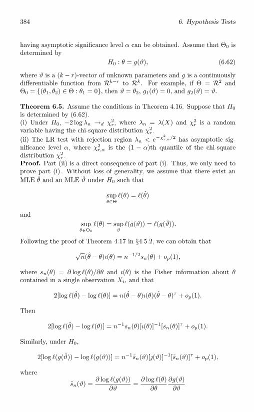
384 6. Hypothesis Tests
having asymptotic significance level α can be obtained. Assume that Θ0 isdetermined by
H0 : θ = g(ϑ), (6.62)
where ϑ is a (k− r)-vector of unknown parameters and g is a continuouslydifferentiable function from Rk−r to Rk. For example, if Θ = R2 andΘ0 = (θ1, θ2) ∈ Θ : θ1 = 0, then ϑ = θ2, g1(ϑ) = 0, and g2(ϑ) = ϑ.
Theorem 6.5. Assume the conditions in Theorem 4.16. Suppose that H0is determined by (6.62).(i) Under H0, −2 log λn →d χ2
r, where λn = λ(X) and χ2r is a random
variable having the chi-square distribution χ2r.
(ii) The LR test with rejection region λn < e−χ2r,α/2 has asymptotic sig-
nificance level α, where χ2r,α is the (1 − α)th quantile of the chi-square
distribution χ2r.
Proof. Part (ii) is a direct consequence of part (i). Thus, we only need toprove part (i). Without loss of generality, we assume that there exist anMLE θ and an MLE ϑ under H0 such that
supθ∈Θ
(θ) = (θ)
andsupθ∈Θ0
(θ) = supϑ
(g(ϑ)) = (g(ϑ)).
Following the proof of Theorem 4.17 in §4.5.2, we can obtain that
√n(θ − θ)ı(θ) = n−1/2sn(θ) + op(1),
where sn(θ) = ∂ log (θ)/∂θ and ı(θ) is the Fisher information about θcontained in a single observation Xi, and that
2[log (θ) − log (θ)] = n(θ − θ)ı(θ)(θ − θ)τ + op(1).
Then
2[log (θ) − log (θ)] = n−1sn(θ)[ı(θ)]−1[sn(θ)]τ + op(1).
Similarly, under H0,
2[log (g(ϑ)) − log (g(ϑ))] = n−1sn(ϑ)[j(ϑ)]−1[sn(ϑ)]τ + op(1),
where
sn(ϑ) =∂ log (g(ϑ))
∂ϑ=
∂ log (θ)∂θ
∂g(ϑ)∂ϑ
6.4. Tests in Parametric Models 385
and j(ϑ) is the Fisher information about ϑ (under H0) contained in Xi.Combining these results, we obtain that
−2 log λn = 2[log (θ) − log (g(ϑ))]= n−1sn(g(ϑ))B(ϑ)[sn(g(ϑ))]τ + op(1)
under H0, where
B(ϑ) = [ı(g(ϑ))]−1 −D(ϑ)[j(ϑ)]−1[D(ϑ)]τ
and D(ϑ) = ∂g(ϑ)/∂ϑ. By the CLT, n−1/2sn(θ) →d Nk
(0, ı(θ)
). Then, it
follows from Theorem 1.10(iii) that, under H0,
−2 log λn →d Z[ı(g(ϑ))]1/2B(ϑ)[ı(g(ϑ))]1/2Zτ ,
where Z = Nk(0, Ik). Let D = D(ϑ), B = B(ϑ), A = ı(g(ϑ)), and C =j(ϑ). Then
(A1/2BA1/2)2 = A1/2BABA1/2
= A1/2(A−1 −DC−1Dτ )A(A−1 −DC−1Dτ )A1/2
= (Ik −A1/2DC−1DτA1/2)(Ik −A1/2DC−1DτA1/2)= Ik − 2A1/2DC−1DτA1/2 + A1/2DC−1DτADC−1DτA1/2
= Ik −A1/2DC−1DτA1/2
= A1/2BA1/2,
where the next to last equality follows from the fact that C = DτAD. Thisshows that A1/2BA1/2 is a projection matrix. The rank of A1/2BA1/2 is
tr(A1/2BA1/2) = tr(Ik −DC−1DτA)= k − tr(C−1DτAD)= k − tr(C−1C)= k − (k − r)= r.
Thus, there is an orthogonal matrix Γ such that
A1/2BA1/2 = Γ(
Ir 00 0
)Γτ .
Since ZΓ = Nk(0, Ik), Z[ı(g(ϑ))]1/2B(ϑ)[ı(g(ϑ))]1/2Zτ = χ2r.
As an example, Theorem 6.5 can be applied to testing problems inExample 4.33 where the exact rejection region of the LR test of size α isdifficult to obtain but the likelihood ratio λn can be calculated numerically.
386 6. Hypothesis Tests
Tests whose rejection regions are constructed using asymptotic theory(so that these tests have asymptotic significance level α) are called asymp-totic tests, which are useful when a test of exact size α is difficult to find.There are two popular asymptotic tests based on likelihoods that are asymp-totically equivalent to LR tests. Note that the hypothesis in (6.62) is equiv-alent to a set of r ≤ k equations:
H0 : R(θ) = 0, (6.63)
where R(θ) is a continuously differentiable function from Rk to Rr. Wald(1943) introduced a test that rejects H0 if and only if Wn > c, where
Wn = R(θ)C(θ)[In(θ)]−1[C(θ)]τ−1[R(θ)]τ ,
In(θ) is the Fisher information matrix based on X1, ..., Xn, θ is an MLE orRLE of θ, and C(θ) = ∂R(θ)/∂θ.
Rao (1947) introduced a score test that rejects H0 if and only if Rn > c,where
Rn = sn(g(ϑ))[In(g(ϑ))]−1[sn(g(ϑ))]τ ,
g is given in (6.62), sn(θ) = ∂ log (θ)/∂θ is the score function, and ϑ is anMLE or RLE of ϑ under H0 in (6.62).
Theorem 6.6. Assume the conditions in Theorem 4.16.(i) Suppose that H0 is determined by (6.63). Under H0, Wn →d χ2
r and,therefore, the test rejects H0 if and only if Wn > χ2
r,α has asymptoticsignificance level α, where χ2
r,α is the (1 − α)th quantile of the chi-squaredistribution χ2
r.(ii) Suppose that H0 is determined by (6.62). Under H0, Rn →d χ2
r and,therefore, the test rejects H0 if and only if Rn > χ2
r,α has asymptoticsignificance level α.Proof. (i) Using Theorems 1.12 and 4.17,
√n[R(θ) −R(θ)] →d Nr(0, C(θ)[ı(θ)]−1[C(θ)]τ ),
where ı(θ) = n−1In(θ). Under H0, R(θ) = 0 and, therefore,
nR(θ)C(θ)[ı(θ)]−1[C(θ)]τ−1[R(θ)]τ →d χ2r
(Theorem 1.10). The result follows from
C(θ)[ı(θ)]−1[C(θ)]τ →p C(θ)[ı(θ)]−1[C(θ)]τ ,
since both ı(θ) and C(θ) are continuous at θ.(ii) The proof of a special case is given as an exercise. For the proof of thegeneral case, see Sen and Singer (1993, pp. 242-244).
6.4. Tests in Parametric Models 387
Thus, Wald’s tests, Rao’s score tests, and LR tests are asymptoticallyequivalent. Note that Wald’s test requires computing θ, not ϑ, whereasRao’s score test requires computing ϑ, not θ. On the other hand, an LR testrequires computing both θ and ϑ (or solving two maximization problems).Hence, one may choose one of these tests which is easy to compute in aparticular application.
The results in Theorems 6.5 and 6.6 can be extended to non-i.i.d. sit-uations (e.g., the GLM in §4.4.2). We state without proof the followingresult.
Theorem 6.7. Assume the conditions in Theorem 4.18. Consider theproblem of testing H0 in (6.63) (or equivalently, (6.62)) with θ = (β, φ).Then the results in Theorems 6.5 and 6.6 still hold.
Example 6.22. Consider the GLM (4.55)-(4.58) with ti’s in a fixed interval(t0, t∞), 0 < t0 ≤ t∞ < ∞. Then the Fisher information matrix
In(θ) =(
φ−1Mn(β) 00 In(β, φ)
),
where Mn(β) is given by (4.60) and In(β, φ) is the Fisher information aboutφ.
Consider the problem of testing H0 : β = β0 versus H1 : β = β0, whereβ0 is a fixed vector. Let (β, φ) be the MLE (or RLE) of (β, φ). Then,Wald’s test is based on
Wn = (β − β0)Mn(β)(β − β0)τ/φ
and Rao’s score test is based on
Rn = sn(β0)[Mn(β0)]−1[sn(β0)]τ/φ,
where sn(β) is given by (4.65) and φ is a solution of ∂ log (β0, φ)/∂φ = 0.It follows from Theorem 4.18 that both Wn and Rn are asymptoticallydistributed as χ2
r under H0.
Wald’s tests, Rao’s score tests, and LR tests are typically consistent ac-cording to Definition 2.13(iii). They are also Chernoff-consistent (Definition2.13(iv)) if α is chosen to be αn → 0 and χ2
r,αn= o(n) as n → ∞ (exercise).
Other asymptotic optimality properties of these tests are discussed in Wald(1943); see also Serfling (1980, Chapter 10).
6.4.3 χ2-tests
A test that is related to the asymptotic tests described in §6.4.2 is theso-called χ2-test for testing cell probabilities in a multinomial distribu-
388 6. Hypothesis Tests
tion. Consider a sequence of n independent trials with k possible out-comes for each trial. Let pj > 0 be the cell probability of occurrence ofthe jth outcome in any given trial and Xj be the number of occurrencesof the jth outcome in n trials. Then X = (X1, ..., Xk) has the multino-mial distribution (Example 2.7) with the parameter P = (p1, ..., pk). Letξi = (0, ..., 0, 1, 0, ..., 0), where the single nonzero component 1 is located inthe jth position if the ith trial yields the jth outcome. Then ξ1, ..., ξn arei.i.d. and X/n = ξ =
∑ni=1 ξi/n. By the CLT,
Zn(P) =√n(Xn − P
)=
√n(ξ − P) →d Nk(0,Σ), (6.64)
where Σ = Var(X/√n) is a symmetric k × k matrix whose ith diagonal
element is pi(1 − pi) and (i, j)th off-diagonal element is −pipj .Consider the problem of testing
H0 : P = P0 versus H1 : P = P0, (6.65)
where P0 = (p01, ..., p0k) is a known vector of cell probabilities. A populartest for (6.65) is based on the following χ2-statistic:
χ2 =k∑
j=1
(Xj − np0j)2
np0j= ‖Zn(P0)D(P0)‖2, (6.66)
where Zn(P) is given by (6.64) and D(P) is the k × k diagonal matrixwhose jth diagonal element is p
−1/2i . Another popular test is based on the
following modified χ2-statistic:
χ2 =k∑
j=1
(Xj − np0j)2
Xj= ‖Zn(P0)D(X/n)‖2. (6.67)
Note that X/n is an unbiased estimator of P.
Theorem 6.8. Let φ = (√p1, ...,
√pk) and Λ be a k×k projection matrix.
(i) If φΛ = aφ, then
Zn(P)D(P)Λ[Zn(P)D(P)]τ →d χ2r,
where χ2r has the chi-square distribution χ2
r with r = tr(Λ) − a.(ii) The same result holds if D(P) in (i) is replaced by D(X/n).Proof. (i) Let D = D(P), Zn = Zn(P), and Z = Nk(0, Ik). From (6.64)and Theorem 1.10,
ZnDΛ(ZnD)τ →d ZAZτ with A = Σ1/2DΛDΣ1/2.
6.4. Tests in Parametric Models 389
Following the proof of Theorem 6.5, the result in (i) follows if we can showthat A2 = A (i.e., A is a projection matrix) and r = tr(A). Since Λ is aprojection matrix and φΛ = aφ, a must be either 0 or 1. Note that
DΣD = Ik − φτφ.
Then
A3 = Σ1/2DΛDΣDΛDΣDΛDΣ1/2
= Σ1/2D(Λ − aφτφ)(Λ − aφτφ)ΛDΣ1/2
= Σ1/2D(Λ − 2aφτφ + a2φτφ)ΛDΣ1/2
= Σ1/2D(Λ − aφτφ)ΛDΣ1/2
= Σ1/2DΛDΣDΛDΣ1/2
= A2,
which implies that the eigenvalues of A must be 0 or 1. Therefore, A2 = A.Also,
tr(A) = tr[Λ(DΣD)] = tr(Λ − aφτφ) = tr(Λ) − a.
(ii) The result in (ii) follows from the result in (i) and the fact that X/n →p
P.
Note that the χ2-statistic in (6.66) and the modified χ2-statistic in (6.67)are special cases of the statistics in Theorem 6.8(i) and (ii), respectively,with Λ = Ik satisfying φΛ = φ. Hence, a test of asymptotic significancelevel α for testing (6.65) rejects H0 when χ2 > χ2
k−1,α (or χ2 > χ2k−1,α),
where χ2k−1,α is the (1 − α)th quantile of χ2
k−1. These tests are called(asymptotic) χ2-tests.
Example 6.23 (Goodness of fit tests). Let Y1, ..., Yn be i.i.d. from F .Consider the problem of testing
H0 : F = F0 versus H1 : F = F0, (6.68)
where F0 is a known c.d.f. For instance, F0 = N(0, 1). One way to test(6.68) is to partition the range of Y1 into k disjoint events A1, ..., Ak andtest (6.65) with pj = PF (Aj) and p0j = PF0(Aj), j = 1, ..., k. Let Xj bethe number of Yi’s in Aj , j = 1, ..., k. Based on Xj ’s, the χ2-tests discussedpreviously can be applied to this problem and they are called goodness offit tests.
In the goodness of fit tests discussed in Example 6.23, F0 in H0 is knownso that p0j ’s can be computed. In some cases we need to test the followinghypotheses that are slightly different from those in (6.68):
H0 : F = Fθ versus H1 : F = Fθ, (6.69)
390 6. Hypothesis Tests
where θ is an unknown parameter in Θ ⊂ Rs. For example, Fθ = N(µ, σ2),θ = (µ, σ2). If we still try to test (6.65) with pj = PFθ
(Aj), j = 1, ..., k, theresult in Example 6.23 is not applicable since P is unknown under H0. Ageneralized χ2-test for (6.69) can be obtained using the following result. LetP(θ) = (p1(θ), ..., pk(θ)) be a k-vector of known functions of θ ∈ Θ ⊂ Rs,where s < k. Consider the testing problem
H0 : P = P(θ) versus H1 : P = P(θ). (6.70)
Note that (6.65) is the special case of (6.70) with s = 0, i.e., θ is known.Let θ be an MLE of θ under H0. Then, by Theorem 6.5, the LR test thatrejects H0 when −2 log λn > χ2
k−s−1,α has asymptotic significance level α,where χ2
k−s−1,α is the (1 − α)th quantile of χ2k−s−1 and
λn =k∏
j=1
[pj(θ)]Xj
/(Xj/n)Xj .
Using the fact that pj(θ)/(Xj/n) →p 1 under H0 and
log(1 + x) = x− x2/2 + o(|x|2) as |x| → 0,
we obtain that
−2 log λn = −2k∑
j=1
Xj log
(1 +
pj(θ)Xj/n
− 1
)
= −2k∑
j=1
Xj
(pj(θ)Xj/n
− 1
)+
k∑j=1
Xj
(pj(θ)Xj/n
− 1
)2
+ op(1)
=k∑
j=1
[Xj − npj(θ)]2
Xj+ op(1)
=k∑
j=1
[Xj − npj(θ)]2
npj(θ)+ op(1),
where the third equality follows from∑k
j=1 pj(θ) =∑k
j=1 Xj/n = 1. De-fine the generalized χ2-statistics χ2 and χ2 to be the χ2 and χ2 in (6.66)and (6.67), respectively, with p0j ’s replaced by pj(θ)’s. We then have thefollowing result.
Theorem 6.9. Under H0 given by (6.70), the generalized χ2-statisticsconverge in distribution to χ2
k−s−1. The χ2-test with rejection region χ2 >χ2k−s−1,α (or χ2 > χ2
k−s−1,α) has asymptotic significance level α, whereχ2k−s−1,α is the (1 − α)th quantile of χ2
k−s−1.
6.4. Tests in Parametric Models 391
Theorem 6.9 can be applied to derive a goodness of fit test for hypotheses(6.69). However, one has to formulate (6.70) and compute an MLE of θunder H0 : P = P(θ), which is different from an MLE under H0 : F = Fθ
unless (6.69) and (6.70) are the same; see Moore and Spruill (1975). Thenext example is the main application of Theorem 6.9.
Example 6.24 (r× c contingency tables). In Example 6.12 we consideredthe 2 × 2 contingency table. The following r × c contingency table is anatural extension:
A1 A2 · · · Ac TotalB1 X11 X12 · · · X1c n1
B2 X21 X22 · · · X2c n2
· · · · · · · · · · · · · · · · · ·Br Xr1 Xr2 · · · Xrc nr
Total m1 m2 · · · mc n
where Ai’s are disjoint events with A1 ∪ · · · ∪ Ac = Ω (the sample spaceof a random experiment), Bi’s are disjoint events with B1 ∪ · · · ∪ Br = Ω,and Xij is the observed frequency of the outcomes in Aj ∩ Bi. Similar tothe case of the 2 × 2 contingency table discussed in Example 6.12, thereare two important applications in this problem. We first consider testingindependence of Aj : j = 1, ..., c and Bi : i = 1, ..., r with hypotheses
H0 : pij = piqj for all i, j versus H1 : pij = piqj for some i, j,
where pij = P (Aj ∩ Bi) = E(Xij)/n, pi = P (Bi), and qj = P (Aj), i =1, ..., r, j = 1, ..., c. In this case, X = (Xij , i = 1, ..., r, j = 1, ..., c) hasthe multinomial distribution with parameters pij , i = 1, ..., r, j = 1, ..., c.Under H0, MLE’s of pi’s and qj ’s are Xi· = ni/n and X·j = mj/n, i =1, ..., r, j = 1, ..., c (exercise). By Theorem 6.9, the χ2-test rejects H0 whenχ2 > χ2
(r−1)(c−1),α, where
χ2 =r∑
i=1
c∑j=1
(Xij − nXi·X·j)2
nXi·X·j(6.71)
and χ2(r−1)(c−1),α is the (1 − α)th quantile of the chi-square distribution
χ2(r−1)(c−1) (exercise). One can also obtain the modified χ2-test by replacing
nXi·X·j by Xij in the denominator of each term of the sum in (6.71).Next, suppose that (X1j , ..., Xrj), j = 1, ..., c, are c independent random
vectors having the multinomial distributions with parameters (p1j , ..., prj),j = 1, ..., c, respectively. Consider the problem of testing whether c multi-nomial distributions are the same, i.e.,
H0 : pij = pi1 for all i, j versus H1 : pij = pi1 for some i, j.
392 6. Hypothesis Tests
It turns out that the rejection region of the χ2-test given in Theorem 6.9 isstill χ2 > χ2
(r−1)(c−1),α with χ2 given by (6.71) (exercise).One can also obtain the LR test in this problem. When r = c = 2,
the LR test is equivalent to Fisher’s test given in Example 6.12, which is aUMPU test. When r > 2 or c > 2, however, a UMPU test does not existin this problem.
6.4.4 Bayes tests
An LR test actually compares supθ∈Θ0(θ) with supθ∈Θ1
(θ) for testing(6.59). Instead of comparing two maximum values, one may compare twoaverages such as πj =
∫Θj
(θ)dΠ(θ)/∫Θ (θ)dΠ(θ), j = 0, 1, where Π(θ) is
a c.d.f. on Θ, and reject H0 when π1 > π0. If Π is treated as a prior c.d.f.,then πj is the posterior probability of Θj , and this test is a particular Bayesaction (see Exercise 13 in §4.6) and is called a Bayes test.
In Bayesian analysis one often considers the Bayes factor defined to be
β =posterior odds ratio
prior odds ratio=
π0/π1
π0/π1,
where πj = Π(Θj) is the prior probability of Θj .Clearly, if there is a statistic sufficient for θ, then the Bayes test and
Bayes factor depend only on the sufficient statistic.Consider the special case where Θ0 = θ0 and Θ1 = θ1 are simple
hypotheses. Then Π(Θj) = πj and, for given X = x,
πj =πjfθj (x)
π0fθ0(x) + π1fθ1(x).
Rejecting H0 when π1 > π0 is the same as rejecting H0 when
fθ1(x)fθ0(x)
>π0
π1. (6.72)
This is equivalent to the UMP test T∗ in (6.3) (Theorem 6.1) with c = π0/π1and γ = 0. The Bayes factor in this case is
β =π0π1
π1π0=
fθ1(x)fθ0(x)
.
Thus, the UMP test T∗ in (6.3) is equivalent to the test using the Bayesfactor. Note that the rejection region given by (6.72) depends on priorprobabilities whereas the Bayes factor does not.
When either Θ0 or Θ1 is not simple, however, Bayes factors also dependon the prior Π.
6.4. Tests in Parametric Models 393
If Π is an improper prior, the Bayes test is still defined as long as theposterior probabilities πj are finite. However, the Bayes factor is not welldefined when Π is improper.
Example 6.25. Let X1, ..., Xn be i.i.d. from N(µ, σ2) with an unknownµ ∈ R and a known σ2 > 0. Let the prior of µ be N(ξ, τ2). Then theposterior of µ is N(µ∗(x), c2), where
µ∗(x) =σ2
nτ2 + σ2 ξ +nτ2
nτ2 + σ2 x and c2 =τ2σ2
nτ2 + σ2
(see Example 2.25). Consider first the problem of testing H0 : µ ≤ µ0versus H1 : µ > µ0. Let Φ be the c.d.f. of the standard normal. Then theposterior probability of Θ0 and the Bayes factor are, respectively,
π0 = Φ(
µ0−µ∗(x)c
)and β =
Φ(
µ0−µ∗(x)c
)Φ(
µ0−ξ
τ
)Φ(
µ∗(x)−µ0c
)Φ(
ξ−µ0τ
) .It is interesting to see that if we let τ → ∞, which is the same as consideringthe improper prior Π = the Lebesgue measure on R, then
π0 → Φ(
µ0−xσ/
√n
),
which is exactly the p-value α(x) derived in Example 2.29.Consider next the problem of testing H0 : µ = µ0 versus H1 : µ = µ0.
In this case the prior c.d.f. can not be continuous at µ0. We considerΠ(µ) = π0I[µ0,∞)(µ) + (1− π0)Φ
(µ−ξτ
). Let (µ) be the likelihood function
based on x. Then
m1(x) =∫µ =µ0
(µ)dΦ(
µ−ξτ
)= 1√
τ2+σ2/nΦ′
(x−ξ√
τ2+σ2/n
),
where Φ′(t) is p.d.f. of the standard normal distribution, and
π0 =π0(µ0)
π0(µ0) + (1 − π0)m1(x)=
(1 +
1 − π0
π0β
)−1
,
where
β =(µ0)m1(x)
=
√nτ2 + σ2Φ′
(x−µ0σ/
√n
)σΦ′
(x−ξ√
τ2+σ2/n
)is the Bayes factor.
More discussions about Bayesian hypothesis tests can be found in Berger(1985, §4.3.3).
394 6. Hypothesis Tests
6.5 Tests in Nonparametric Models
In a nonparametric problem, a UMP, UMPU, or UMPI test usually does notexist. In this section we study some nonparametric tests that have size α,limiting size α, or asymptotic significance level α. Consistency (Definition2.13) of these nonparametric tests is also discussed.
Nonparametric tests are derived using some intuitively appealing ideas.They are commonly referred to as distribution-free tests, since almost noassumption is imposed on the population under consideration. But a non-parametric test may not be as good as a parametric test (in terms of itspower) when the parametric model is correct. This is very similar to thecase where we consider parametric estimation methods versus nonparamet-ric estimation methods.
6.5.1 Sign, permutation, and rank tests
Three popular classes of nonparametric tests are introduced here. The firstone is the class of sign tests. Let X1, ..., Xn be i.i.d. random variables fromF , u be a fixed constant, and p = F (u). Consider the problem of testingH0 : p ≤ p0 versus H1 : p > p0, or testing H0 : p = p0 versus H1 : p = p0,where p0 is a fixed constant in (0, 1). Let
∆i =
1 Xi − u ≤ 00 Xi − u > 0,
i = 1, ..., n.
Then ∆1, ...,∆n are i.i.d. binary random variables with p = P (∆i = 1).For testing H0 : p ≤ p0 versus H1 : p > p0, it follows from Corollary 6.1that the test
T∗(Y ) =
⎧⎨⎩1 Y > m
γ Y = m
0 Y < m
(6.73)
is of size α and UMP among tests based on ∆i’s, where Y =∑n
i=1 ∆i
and m and γ satisfy (6.7). Although T∗ is of size α, we cannot concludeimmediately that T∗ is a UMP test, since ∆1, ...,∆n may not be sufficientfor F . However, it can be shown that T∗ is in fact a UMP test (Lehmann,1986, pp. 106-107) in this particular case. Note that no assumption isimposed on F .
For testing H0 : p = p0 versus H1 : p = p0, it follows from Theorem 6.4that the test
T∗(Y ) =
⎧⎨⎩1 Y < c1 or Y > c2γi Y = ci, i = 1, 2,0 c1 < Y < c2
(6.74)
6.5. Tests in Nonparametric Models 395
is of size α and UMP among unbiased tests based on ∆i’s, where γ and ci’sare chosen so that Ep=p0(T∗) = α and Ep=p0(T∗Y ) = αnp0. This test is infact a UMPU test (Lehmann, 1986, p. 166).
Since Y is equal to the number of nonnegative signs of (u−Xi)’s, testsbased on T∗ in (6.73) or (6.74) are called sign tests. One can easily extendthe sign tests to the case where p = P (X1 ∈ B) with any fixed event B.Another extension is to the case where we observe i.i.d. (X1, Y1), ..., (Xn, Yn)(matched pairs). By using ∆i = Xi − Yi − u, one can obtain sign tests forhypotheses concerning P (X1 − Y1 ≤ u).
Next, we introduce the class of permutation tests. Let Xi1, ..., Xini ,i = 1, 2, be two independent samples i.i.d. from Fi, i = 1, 2, respectively,where Fi’s are c.d.f.’s on R. In §6.2.3, we showed that the two-samplet-tests are UMPU tests for testing hypotheses concerning the means ofFi’s, under the assumption that Fi’s are normal with the same variance.Such types of testing problems arise from the comparison of two treatments.Suppose now we remove the normality assumption and replace it by a muchweaker assumption that Fi’s are in the nonparametric family F containingall continuous c.d.f.’s on R. Consider the problem of testing
H0 : F1 = F2 versus H1 : F1 = F2, (6.75)
which is the same as testing the equality of the means of Fi’s when Fi’s arenormal with the same variance.
Let X = (Xij , j = 1, ..., ni, i = 1, 2), n = n1 + n2, and α be a givensignificance level. A test T (X) satisfying
1n!
∑z∈π(x)
T (z) = α (6.76)
is called a permutation test, where π(x) is the set of n! points obtainedfrom x ∈ Rn by permuting the components of x. Permutation tests areof size α (exercise). Under the assumption that F1(x) = F2(x − θ) andF1 ∈ F containing all c.d.f.’s having Lebesgue p.d.f.’s that are continuousa.e., which is still much weaker than the assumption that Fi’s are normalwith the same variance, the class of permutation tests of size α is exactlythe same as the class of unbiased tests of size α; see, for example, Lehmann(1986, p. 231).
Unfortunately, a test UMP among all permutation tests of size α doesnot exist. In applications, we usually choose a Lebesgue p.d.f. h and definea permutation test
T (X) =
⎧⎨⎩1 h(X) > hm
γ h(X) = hm
0 h(X) < hm,
(6.77)
396 6. Hypothesis Tests
where hm is the (m + 1)th largest value of the set h(z) : z ∈ π(x), m isthe integer part of αn!, and γ = αn!−m. This permutation test is optimalin some sense (Lehmann, 1986, §5.11).
While the class of permutation tests is motivated by the unbiasednessprinciple, the third class of tests introduced here is motivated by the in-variance principle.
Consider first the one-sample problem in which X1, ..., Xn are i.i.d. ran-dom variables from a continuous c.d.f. F and we would like to test
H0 : F is symmetric about 0 versus H1 : F is not symmetric about 0.
Let G be the class of transformations g(x) = (ψ(x1), ..., ψ(xn)), where ψ iscontinuous, odd, and strictly increasing. Let R(X) be the vector of ranks of|Xi|’s and R+(X) (or R−(X)) be the subvector of R(X) containing rankscorresponding to positive (or negative) Xi’s. It can be shown (exercise) that(R+, R−) is maximal invariant under G. Furthermore, sufficiency permitsa reduction from R+ and R− to Ro
+, the vector of ordered components ofR+. A test based on Ro
+ is called a (one-sample) signed rank test.Similar to the case of permutation tests, there is no UMP test within
the class of signed rank tests. A common choice is the signed rank test thatrejects H0 when W (Ro
+) is too large or too small, where
W (Ro+) = J(Ro
+1/n) + · · · + J(Ro+n∗/n), (6.78)
J is a continuous and strictly increasing function on [0, 1], Ro+i is the ith
component of Ro+, and n∗ is the number of positive Xi’s. This is motivated
by the fact that H0 is unlikely to be true if W in (6.78) is too large or toosmall. Note that W/n is equal to T(Fn) with T given by (5.46) and J(t) = t,and the test based on W in (6.78) is the well-known one-sample Wilcoxonsigned rank test.
Under H0, P (Ro+ = y) = 2−n for each y ∈ Y containing 2n n∗-tuples
y = (y1, ..., yn∗) satisfying 1 ≤ y1 < · · · < yn∗ ≤ n. Then, the followingsigned rank test is of size α:
T (X) =
⎧⎨⎩1 W (Ro
+) < c1 or W (Ro+) > c2
γ W (Ro+) = ci, i = 1, 2
0 c1 < W (Ro+) < c2,
(6.79)
where c1 and c2 are the (m + 1)th smallest and largest values of the setW (y) : y ∈ Y, m is the integer part of α2n/2, and γ = α2n/2 −m.
Consider next the two-sample problem of testing (6.75) based on twoindependent samples, Xi1, ..., Xini , i = 1, 2, i.i.d. from Fi, i = 1, 2, respec-tively. Let G be the class of transformations g(x) = (ψ(xij), j = 1, ..., ni, i =
6.5. Tests in Nonparametric Models 397
1, 2), where ψ is continuous and strictly increasing. Let R(X) be the vec-tor of ranks of all Xij ’s. In Example 6.14, we showed that R is maximalinvariant under G. Again, sufficiency permits a reduction from R to Ro
1,the vector of ordered values of the ranks of X11, ..., X1n1 . A test for (6.75)based on Ro
1 is called a two-sample rank test. Under H0, P (Ro1 = y) =(
nn1
)−1 for each y ∈ Y containing(nn1
)n1-tuples y = (y1, ..., yn1) satisfying
1 ≤ y1 < · · · < yn1 ≤ n. Let Ro1 = (Ro
11, ..., Ro1n1
). Then a commonlyused two-sample rank test is given by (6.78)-(6.79) with Ro
+i, n∗, and 2n
replaced by Ro1i, n1, and
(nn1
), respectively. When n1 = n2, the statistic
W/n is equal to T(Fn) with T given by (5.48). When J(t) = t − 12 , this
reduces to the well-known two-sample Wilcoxon rank test.A common feature of the permutation and rank tests previously intro-
duced is that tests of size α can be obtained for each fixed sample size n, butthe computation involved in determining the rejection regions T (X) = 1may be cumbersome if n is large. Thus, one may consider approximationsto permutation and rank tests when n is large. Permutation tests can of-ten be approximated by the two-sample t-tests derived in §6.2.3 (Lehmann,1986, §5.13). Using the results in §5.2.2, we now derive one-sample signedrank tests having limiting size α (Definition 2.13(ii)), which can be viewedas signed rank tests of size approximately α when n is large.
From the discussion in §5.2.2, W/n = T(Fn) with a ∞-Hadamard dif-ferentiable functional T given by (5.46) and, by Theorem 5.5,
√n[W/n− T(F )] →d N(0, σ2
F ),
where σ2F = E[φF (X1)]2 and
φF (x) =∫ ∞
0J ′(F (y))(δx − F )(y)dF (y) + J(F (x)) − T(F )
(see (5.47)). Since F is continuous, F (x) = F (x) − F (−x). Under H0,F (x) = 1 − F (−x). Hence, σ2
F under H0 is equal to v1 + v2 + 2v12, where
v1 = Var(J(F (X1))
)=
12
∫ ∞
0[J(F (x))]2dF (x),
v2 = Var(∫ ∞
0J ′(F (y))(δX1 − F )(y)dF (y)
)= E
∫ ∞
0
∫ ∞
0J ′(F (y))J ′(F (z))(δX1 − F )(y)(δX1 − F )(z)dF (y)dF (z)
=14
∫ ∞
0
∫ ∞
0J ′(F (y))J ′(F (z))[F (min(y, z)) − F (y)F (z)]dF (y)dF (z)
=12
∫0<z<y<∞
J ′(F (y))J ′(F (z))F (z)[1 − F (y)]dF (y)dF (z),
398 6. Hypothesis Tests
and
v12 = Cov(J(F (X1)),
∫ ∞
0J ′(F (y))(δX1 − F )(y)dF (y)
)= E
∫ ∞
0J(F (X1))J ′(F (y))(δX1 − F )(y)dF (y)
=∫ ∞
−∞
∫ ∞
0J(F (x))J ′(F (y))(δ|x| − F )(y)dF (y)dF (x)
=12
∫ ∞
0
∫ ∞
0J(F (x))J ′(F (y))(δx − F )(y)dF (y)dF (x).
Note that under H0, the distribution of W is completely known. Indeed,letting s = F (y) and t = F (z), we conclude that σ2
F = v1 + v2 + 2v12 and
T(F ) =∫ ∞
0J(F (x))dF (x) =
12
∫ 1
0J(s)ds
do not depend on F . Hence, a signed rank test T that rejects H0 when√n|W/n− t0| > σ0z1−α/2, (6.80)
where za = Φ−1(a) and t0 = T(F ) and σ20 = σ2
F under H0 are knownconstants, has the property that
supP∈P0
βT (P ) = supP∈P0
P(√
n|W/n− t0| > σ0z1−α/2)
= PW
(√n|W/n− t0| > σ0z1−α/2
)→ α,
i.e., T has limiting size α.Two-sample rank tests having limiting size α can be similarly derived
(exercise).
6.5.2 Kolmogorov-Smirnov and Cramer-von Mises tests
In this section we introduce two types of tests for hypotheses concerningcontinuous c.d.f.’s on R. Let X1, ..., Xn be i.i.d. random variables from acontinuous c.d.f. F . Suppose that we would like to test hypotheses (6.68),i.e., H0 : F = F0 versus H1 : F = F0 with a fixed F0. Let Fn be theempirical c.d.f. and
Dn(F ) = supx∈R
|Fn(x) − F (x)|, (6.81)
which is in fact the distance ∞(Fn, F ). Intuitively, Dn(F0) should be smallif H0 is true. From the results in §5.1.1 we know that Dn(F0) →a.s. 0 if and
6.5. Tests in Nonparametric Models 399
only if H0 is true. The statistic Dn(F0) is called the Kolmogorov-Smirnovstatistic. Tests with rejection region Dn(F0) > c are called Kolmogorov-Smirnov tests.
In some cases we would like to test “one-sided” hypotheses H0 : F = F0versus H1 : F ≥ F0, F = F0, or H0 : F = F0 versus H1 : F ≤ F0, F = F0.The corresponding Kolmogorov-Smirnov statistic is D+
n (F0) or D−n (F0),
whereD+
n (F ) = supx∈R
[Fn(x) − F (x)] (6.82)
andD−
n (F ) = supx∈R
[F (x) − Fn(x)].
The rejection regions of one-sided Kolmogorov-Smirnov tests are, respec-tively, D+
n (F0) > c and D−n (F0) > c.
Let X(1) < · · · < X(n) be the order statistics and define X(0) = −∞ andX(n+1) = ∞. Since Fn(x) = i/n when X(i) ≤ x < X(i+1), i = 0, 1, ..., n,
D+n (F ) = max
0≤i≤nsup
X(i)≤x<X(i+1)
[i
n− F (x)
]= max
0≤i≤n
[i
n− inf
X(i)≤x<X(i+1)
F (x)]
= max0≤i≤n
[i
n− F (X(i))
].
When F is continuous, F (X(i)) is the ith order statistic of a sample of size nfrom the uniform distribution U(0, 1) irrespective of what F is. Therefore,the distribution of D+
n (F ) does not depend on F , if we restrict our attentionto continuous c.d.f.’s on R. The distribution of D−
n (F ) is the same as thatof D+
n (F ) because of symmetry. Since
Dn(F ) = max[D+n (F ), D−
n (F )],
the distribution of Dn(F ) does not depend on F . This means that thedistributions of Kolmogorov-Smirnov statistics are known under H0.
Theorem 6.10. Let Dn(F ) and D+n (F ) be defined by (6.81) and (6.82).
(i) For any fixed n,
P(D+
n (F ) ≤ t)
=
⎧⎪⎪⎪⎨⎪⎪⎪⎩0 t ≤ 0
n!n∏
i=1
∫ ui+1
in−t
du 0 < t < 1
1 t ≥ 1
400 6. Hypothesis Tests
and
P(Dn(F ) ≤ t
)=
⎧⎪⎪⎪⎨⎪⎪⎪⎩0 t ≤ (2n)−1
n!n∏
i=1
∫ 2i−n−1+t
2i−t
du (2n)−1 < t < 1
1 t ≥ 1,
where du = du1 · · · dun (u1 < · · · < un) and un+1 = 1.(ii) For t > 0,
limn→∞
P(√
nD+n (F ) ≤ t
)= 1 − e−2t2
and
limn→∞
P(√
nDn(F ) ≤ t)
= 1 − 2∞∑j=1
(−1)j−1e−2j2t2 .
The proof of Theorem 6.10(i) is left as an exercise. The proof of Theorem6.10(ii) can be found in Kolmogorov (1933) and Smirnov (1944).
When n is not large, Kolmogorov-Smirnov tests of size α can be obtainedusing the results in Theorem 6.10(i). When n is large, using the results inTheorem 6.10(i) is not convenient. We can obtain Kolmogorov-Smirnovtests of limiting size α using the results in Theorem 6.10(ii).
Another test for H0 : F = F0 versus H1 : F = F0 is the Cramer-vonMises test which rejects H0 when Cn(F0) > c, where
Cn(F ) =∫
[Fn(x) − F (x)]2dF (x) (6.83)
is another measure of disparity between Fn and F . Similar to Dn(F ), thedistribution of Cn(F ) does not depend on F (exercise). Hence, a Cramer-von Mises test of size α can be obtained. When n is large, it is moreconvenient to use a Cramer-von Mises test of limiting size α. Note thatCn(F0) is actually a V-statistic (§3.5.3) with kernel
h(x1, x2) =∫
[δx1(y) − F0(y)][δx2(y) − F0(y)]dF0(y)
and
h1(x1) = E[h(x1, X2)] =∫
[δx1(y) − F0(y)][F (y) − F0(y)]dF0(y).
It follows from Theorem 3.16 that if H1 is true, Cn(F0) is asymptoticallynormal whereas if H0 is true, h1(x1) ≡ 0 and
nCn(F0) →d
∞∑j=1
λjχ21j ,
6.5. Tests in Nonparametric Models 401
where χ21j ’s are i.i.d. from the chi-square distribution χ2
1 and λj ’s are con-stants. In this case, Durbin (1973) showed that λj = j−2π−2.
For testing (6.68), it is worthwhile to compare the goodness of fit testintroduced in Example 6.23 with the Kolmogorov-Smirnov test (or Cramer-von Mises test). The former requires a partition of the range of observationsand may lose information through partitioning, whereas the latter requiresthat F be continuous and univariate; the latter is of size α (or limiting sizeα), whereas the former is only of asymptotic significance level α; the formercan be modified to allow estimation of unknown parameters under H0 (i.e.,hypotheses (6.69)), whereas the latter does not have this flexibility. Notethat goodness of fit tests are nonparametric in nature, although χ2-testsare derived from a parametric model.
Kolmogorov-Smirnov tests can be extended to two-sample problems totest hypotheses in (6.75). Let Xi1, ..., Xini , i = 1, 2, be two indepen-dent samples i.i.d. from Fi on R, i = 1, 2, and let Fini
be the empiricalc.d.f. based on Xi1, ..., Xini . A Kolmogorov-Smirnov test rejects H0 whenDn1,n2 > c, where
Dn1,n2 = supx∈R
|F1n1(x) − F2n2(x)|.
A Kolmogorov-Smirnov test of limiting size α can be obtained using
limn1,n2→∞
P(√
n1n2/(n1 + n2)Dn1,n2 ≤ t)
=∞∑
j=−∞(−1)j−1e−2j2t2 , t > 0.
6.5.3 Empirical likelihood ratio tests
The method of likelihood ratio is useful in deriving tests under parametricmodels. In nonparametric problems, we now introduce a similar methodbased on the empirical likelihoods introduced in §5.1.2.
Suppose that a sample X is from a population determined by a c.d.f.F ∈ F, where F is a class of c.d.f.’s on Rd. Consider the problem of testing
H0 : T(F ) = t0 versus H1 : T(F ) = t0, (6.84)
where T is a functional from F to Rk and t0 is a fixed vector in Rk. Let(G), G ∈ F, be a given empirical likelihood, F be an MELE of F , andFH0 be an MELE of F under H0, i.e., FH0 is an MELE of F subject toT(F ) = t0. Then the empirical likelihood ratio is defined as
λn(X) = (FH0)/(F ).
A test with rejection region λn(X) < c is called an empirical likelihood ratiotest.
402 6. Hypothesis Tests
As a specific example, consider the following empirical likelihood (ornonparametric likelihood) when X = (X1, ..., Xn) with i.i.d. Xi’s:
(G) =n∏
i=1
pi subject to pi ≥ 0,n∑
i=1
pi = 1,
where pi = PG(xi), i = 1, ..., n. Suppose that T(G) =∫u(x)dG(x) with
a known function u(x) from Rd to Rr. Then F = Fn; H0 in (6.84) witht0 = 0 is the same as that assumption (5.9) holds; FH0 is the MELE givenby (5.11); and the empirical likelihood ratio is
λn(X) = nnn∏
i=1
pi, (6.85)
where pi is given by (5.12). An empirical likelihood ratio test with asymp-totic significance level α can be obtained using the following result.
Theorem 6.11. Assume the conditions in Theorem 5.4. Under the hy-pothesis H0 in (6.84) with t0 = 0 (i.e., (5.9) holds),
−2 log λn(X) →d χ2r,
where λn(X) is given by (6.85) and χ2r has the chi-square distribution χ2
r.
The proof of this result can be found in Owen (1988, 1990). In fact,the result in Theorem 6.11 holds for some other functionals T such as themedian functional.
We can also derive tests based on the profile empirical likelihoods dis-cussed in §5.4.1. Consider an empirical likelihood
(G) =n∏
i=1
pi subject to pi ≥ 0,n∑
i=1
pi = 1,n∑
i=1
piψ(xi, θ) = 0,
where θ is a k-vector of unknown parameters and ψ is a known function.Let θ = (ϑ, ϕ), where ϑ is r×1 and ϕ is (k−r)×1. Suppose that we wouldlike to test
H0 : ϑ = ϑ0 versus H1 : ϑ = ϑ0,
where ϑ0 is a fixed r-vector. Let θ be a maximum of the profile empiri-cal likelihood P (θ) given by (5.86) and let ϕ be a maximum of P (ϕ) =P (ϑ0, ϕ). Then a profile empirical likelihood ratio test rejects H0 whenλn(X) < c, where
λn(X) =n∏
i=1
1 + ψ(xi, θ)[ξn(θ)]τ
1 + ψ(xi, ϑ0, ϕ)[ζn(ϑ0, ϕ)]τ, (6.86)
6.5. Tests in Nonparametric Models 403
ξn(θ) satisfiesn∑
i=1
ψ(xi, θ)
1 + ψ(xi, θ)[ξn(θ)]τ= 0
and ζn(ϑ0, ϕ) satisfiesn∑
i=1
ψ(xi, ϑ0, ϕ)1 + ψ(xi, ϑ0, ϕ)[ζn(ϑ0, ϕ)]τ
= 0.
From the discussion in §5.4.1, θ can be approximated by a solution of theGEE
∑ni=1 ψ(Xi, θ) = 0 and ϕ can be approximated by a solution of the
reduced GEE∑n
i=1 ψ(Xi, ϑ0, ϕ) = 0. Under some regularity conditions(e.g., the conditions in Proposition 5.3), Qin and Lawless (1994) showedthat the result in Theorem 6.11 holds with λn(X) given by (6.86). Thus,a profile empirical likelihood ratio test with asymptotic significance level αcan be obtained.
Example 6.26. Let Y1, ..., Yn be i.i.d. random 2-vectors from F . Considerthe problem of testing H0 : µ1 = µ2 versus H1 : µ1 = µ2, where (µ1, µ2) =E(Y1). Let Yi = (Yi1, Yi2), Xi1 = Yi1 − Yi2, Xi2 = Yi1 + Yi2, and Xi =(Xi1, Xi2), i = 1, ..., n. Then X1, ..., Xn are i.i.d. with E(X1) = θ = (ϑ, ϕ),where ϑ = µ1 − µ2 and ϕ = µ1 + µ2. The hypotheses of interest becomesH0 : ϑ = 0 versus H1 : ϑ = 0.
To apply the profile empirical likelihood method, we define ψ(x, θ) =x − θ, x ∈ R2. Note that a solution of the GEE
∑ni=1(Xi − θ) = 0 is
θ = (X1·, X2·) = X, and a solution of the reduced GEE∑n
i=1(X2i−ϕ) = 0is ϕ = X2·. The profile empirical likelihood ratio is then given by
λn(X) =n∏
i=1
1 + (Xi − X)[ξn(X)]τ
1 + [Xi − (0, X2·)][ζn(0, X2·)]τ,
where ξn(X) satisfiesn∑
i=1
Xi − X
1 + (Xi − X)[ξn(X)]τ= 0
and ζn(0, X2·) satisfiesn∑
i=1
Xi − (0, X2·)1 + [Xi − (0, X2·)][ζn(0, X2·)]τ
= 0.
Empirical likelihood ratio tests or profile empirical likelihood ratio testsin various other problems can be found, for example, in Owen (1988, 1990,1991), Chen and Qin (1993), Qin (1993), and Qin and Lawless (1994).
404 6. Hypothesis Tests
6.5.4 Asymptotic tests
We now introduce a simple method of constructing asymptotic tests (i.e.,tests with asymptotic significance level α). This method works for almostall problems (parametric or nonparametric) in which the hypotheses beingtested are H0 : θ = θ0 versus H1 : θ = θ0, where θ is a vector of parameters,and an asymptotically normally distributed estimator of θ can be found.However, this simple method may not provide the best or even nearly bestsolution to the problem, especially when there are different asymptoticallynormally distributed estimators of θ.
Let X be a sample of size n from a population P and θn be an estimatorof θ, a k-vector of parameters related to P . Suppose that under H0,
(θn − θ)V −1/2n →d Nk(0, Ik), (6.87)
where Vn is the asymptotic covariance matrix of θn. If Vn is known whenθ = θ0, then a test with rejection region
(θn − θ0)V −1n (θn − θ0)τ > χ2
k,α (6.88)
has asymptotic significance level α, where χ2k,α is the (1− α)th quantile of
the chi-squared distribution χ2k. If the distribution of θn does not depend
on the unknown population P under H0 and (6.87) holds, then a test withrejection region (6.88) has limiting size α.
If Vn in (6.88) depends on the unknown population P even if H0 is true(θ = θ0), then we have to replace Vn in (6.88) by an estimator Vn. If,under H0, Vn is consistent according to Definition 5.4, then the test havingrejection region (6.88) with Vn replaced by Vn has asymptotic significancelevel α. Variance estimation methods introduced in §5.5 can be used toconstruct a consistent estimator Vn.
In some cases result (6.87) holds for any P . Then, the following resultshows that the test having rejection region (6.88) is asymptotically correct(§2.5.3), i.e., it is a consistent asymptotic test (Definition 2.13).
Theorem 6.12. Assume that (6.87) holds for any P and that λ+[Vn] → 0,where λ+[Vn] is the largest eigenvalue of Vn.(i) The test having rejection region (6.88) (with a known Vn or Vn replacedby an estimator Vn that is consistent for any P ) is consistent.(ii) If we choose α = αn → 0 as n → ∞ and χ2
k,1−αnλ+[Vn] = o(1), then
the test in (i) is Chernoff-consistent.Proof. The proof of (ii) is left as an exercise. We only prove (i) for thecase where Vn is known. Let Zn = (θn − θ)V −1/2
n and ln = (θ − θ0)V−1/2n .
Then ‖Zn‖ = Op(1) and ‖ln‖ = ‖(θ − θ0)V−1/2n ‖ → ∞ when θ = θ0. The
6.5. Tests in Nonparametric Models 405
result follows from the fact that when θ = θ0,
(θn − θ0)V −1n (θn − θ0)τ = ‖Zn‖2 + ‖ln‖2 + 2lnZτ
n
≥ ‖Zn‖2 + ‖ln‖2 − 2‖ln‖‖Zn‖= Op(1) + ‖ln‖2[1 − op(1)]
and, therefore,
P((θn − θ0)V −1
n (θn − θ0)τ > χ2k,α
)→ 1.
Example 6.27. Let X1, ..., Xn be i.i.d. random variables from a symmetricc.d.f. F having finite variance and positive F ′. Consider the problem oftesting H0 : F is symmetric about 0 versus H1 : F is not symmetric about0. Under H0, there are many estimators satisfying (6.87). We consider thefollowing five estimators:(1) θn = X and θ = E(X1);(2) θn = θ0.5 (the sample median) and θ = F−1( 1
2 ) (the median of F );(3) θn = Xa (the a-trimmed sample mean defined by (5.70)) and θ = T(F ),where T is given by (5.39) with J(t) = (1 − 2a)−1I(a,1−a)(t), a ∈ (0, 1
2 );(4) θn = the Hodges-Lehmann estimator (Example 5.8) and θ = F−1( 1
2 );(5) θn = W/n − 1
2 , where W is given by (6.78) with J(t) = t, and θ =T(F ) − 1
2 with T given by (5.46).Although θ in (1)-(5) are different in general, in all cases θ = 0 is
equivalent to that H0 holds.For X, it follows from the CLT that (6.87) holds with Vn = σ2/n for any
F , where σ2 = Var(X1). From the SLLN, S2/n is a consistent estimator ofVn for any F . Thus, the test having rejection region (6.88) with θn = X andVn replaced by S2/n is asymptotically correct. This test is asymptoticallyequivalent to the one-sample t-test derived in §6.2.3.
From Theorem 5.10, θ0.5 satisfies (6.87) with Vn = 4−1[F ′(θ)]−2n−1 forany F . A consistent estimator can be obtained using the bootstrap methodconsidered in §5.5.3. Another consistent estimator of Vn can be obtainedusing the Woodruff’s interval introduced in §7.4 (see Exercise 70 in §7.6).The test having rejection region (6.88) with θn = θ0.5 and Vn replaced bya consistent estimator is asymptotically correct.
It follows from the discussion in §5.3.2 that Xa satisfies (6.87) for anyF . A consistent estimator of Vn can be obtained using formula (5.105)or the jackknife method in §5.5.2. The test having rejection region (6.88)with θn = Xa and Vn replaced by a consistent estimator is asymptoticallycorrect.
From Example 5.8, the Hodges-Lehmann estimator satisfies (6.87) forany F and Vn = 12−1γ−2n−1 under H0, where γ =
∫F ′(x)dF (x). A
406 6. Hypothesis Tests
consistent estimator of Vn under H0 can be obtained using the result inExercise 86 in §5.6. The test having rejection region (6.88) with θn = theHodges-Lehmann estimator and Vn replaced by a consistent estimator isasymptotically correct.
Note that all tests discussed so far are not of limiting size α, since thedistributions of θn are still unknown under H0.
The test having rejection region (6.88) with θn = W/n − 12 and Vn =
(12n)−1 is equivalent to the one-sample Wilcoxon signed rank test and isshown to have limiting size α (§6.5.1). Also, (6.87) is satisfied for any F(§5.2.2). Although Theorem 6.12 is not applicable, a modified proof ofTheorem 6.12 can be used to show the consistency of this test (exercise).
It is not clear which one of the five tests discussed here is to be preferredin general.
The results for θn in (1)-(3) and (5) still hold for testing H0 : θ = 0versus H1 : θ = 0 without the assumption that F is symmetric.
An example of asymptotic tests for one-sided hypotheses is given inExercise 107. Most tests in §6.1-§6.4 derived under parametric models areasymptotically correct even when the parametric model assumptions areremoved. Some examples are given in Exercises 105-107.
Finally, a study of asymptotic efficiencies of various tests can be found,for example, in Serfling (1980, Chapter 10).
6.6 Exercises
1. Prove Theorem 6.1 for the case of α = 0 or 1.
2. Assume the conditions in Theorem 6.1. Let β(P ) be the power func-tion of a UMP test of size α ∈ (0, 1). Show that α < β(P1) unlessP0 = P1.
3. Let T∗ be given by (6.3) with c = c(α) for an α > 0.(a) Show that if α1 < α2, then c(α1) ≥ c(α2).(b) Show that if α1 < α2, then the type II error probability of T∗ ofsize α1 is larger than that of T∗ of size α2.
4. Let H0 and H1 be simple and let α ∈ (0, 1). Suppose that T∗ is aUMP test of size α for testing H0 versus H1 and that β < 1, where βis the power of T∗ when H1 is true. Show that 1 − T∗ is a UMP testof size 1 − β for testing H1 versus H0.
5. Let X be a sample of size 1 from a Lebesgue p.d.f. fθ. Find a UMPtest of size α ∈ (0, 1
2 ) for H0 : θ = θ0 versus H1 : θ = θ1 in the
6.6. Exercises 407
following cases:(a) fθ(x) = 2θ−2(θ − x)I(0,θ)(x), θ0 < θ1;(b) fθ(x) = 2[θx + (1 − θ)(1 − x)]I(0,1)(x), 0 ≤ θ1 < θ0 ≤ 1;(c) fθ0 is the p.d.f. of N(0, 1) and fθ1 is the p.d.f. of the Cauchydistribution C(0, 1);(d) fθ0(x) = 4xI(0, 12 )(x) + 4(1 − x)I( 1
2 ,1)(x) and fθ1(x) = I(0,1)(x);
(e) fθ is the p.d.f. of the Cauchy distribution C(θ, 1), θ0 = 0, andθ1 = 1.
6. Let X1, ..., Xn be i.i.d. from a Lebesgue p.d.f. fθ. Find a UMP testof size α for H0 : θ = θ0 versus H1 : θ = θ1 in the following cases:(a) fθ(x) = e−(x−θ)I(θ,∞)(x), θ0 < θ1;(b) fθ(x) = θx−2I(θ,∞)(x), θ0 = θ1.
7. Prove Lemma 6.1.
8. Let f0 and f1 be Lebesgue integrable functions on R and
φ∗(x) =
1 f0(x) < 0 or f0(x) = 0, f1(x) ≥ 00 f0(x) > 0 or f0(x) = 0, f1(x) < 0.
Show that φ∗ maximizes∫φ(x)f1(x)dx over all functions φ from R
to [0, 1] such that∫φ(x)f0(x)dx =
∫φ∗(x)f0(x)dx.
9. Prove Proposition 6.1.
10. Prove the claims in Example 6.5.
11. Show that the family fθ : θ ∈ R with fθ(x) = c(θ)h(x)I(a(θ),b(θ))(x)has monotone likelihood ratio, where h(x) is a positive Lebesgue in-tegrable function, and a(θ) and b(θ) are nondecreasing functions ofθ.
12. Let X1, ..., Xn be i.i.d. from a p.d.f. fθ, θ ∈ Θ ⊂ R. Find a UMP testof size α for testing H0 : θ ≤ θ0 versus H1 : θ > θ0 in the followingcases:(a) fθ(x) = θ−1e−x/θI(0,∞)(x), θ > 0;(b) fθ(x) = θ−1xθ−1I(0,1)(x), θ > 0;(c) fθ(x) is the p.d.f. of N(1, θ);(d) fθ(x) = θ−ccxc−1e−(x/θ)cI(0,∞)(x), θ > 0, where c > 0 is known.
13. Suppose that the distribution of X is in a family with monotonelikelihood ratio in Y (X), where Y (X) has a continuous distribution.Consider the hypotheses H0 : θ ≤ θ0 versus H1 : θ > θ0. Show thatthe p-value (§2.4.2) of the UMP test is given by Pθ0(Y ≥ y), where yis the observed value of Y .
408 6. Hypothesis Tests
14. Let X1, ..., Xm be i.i.d. from N(µx, σ2x) and Y1, ..., Yn be i.i.d. from
N(µy, σ2y). Suppose that Xi’s and Yj ’s are independent.
(a) When σx = σy = 1, find a UMP test of size α for testing H0 :µx ≤ µy versus H1 : µx > µy. (Hint: see Lehmann (1986, §3.9).)(b) When µx and µy are known, find a UMP test of size α for testingH0 : σx ≤ σy versus H1 : σx > σy. (Hint: see Lehmann (1986, §3.9).)
15. Let f and g be two known p.d.f.’s w.r.t. ν. Suppose that X has thep.d.f. θf(x) + (1 − θ)g(x), θ ∈ R. Show that the test T∗(X) ≡ αis a UMP test of size α for testing H0 : θ ≤ θ1 or θ ≥ θ2 versusH1 : θ1 < θ < θ2.
16. Let X1, ..., Xn be i.i.d. from the uniform distribution U(θ, θ + 1), θ ∈R. Suppose that n ≥ 2.(a) Find the joint distribution of X(1) and X(n).(b) Show that a UMP test of size α for testing H0 : θ ≤ 0 versusH1 : θ > 0 is of the form
T∗(X(1), X(n)) =
0 X(1) < 1 − α1/n, X(n) < 11 otherwise.
(c) Does the family of all possible distributions of (X(1), X(n)) havemonotone likelihood ratio? (Hint: see Lehmann (1986, p. 115).)
17. Suppose that X1, ..., Xn are i.i.d. from the discrete uniform distribu-tion DU(1, ..., θ) (Table 1.1, page 18) with an unknown θ = 1, 2, ....(a) Consider H0 : θ ≤ θ0 versus H1 : θ > θ0. Show that
T∗(X) =
1 X(n) > θ0
α X(n) ≤ θ0
is a UMP test of size α.(b) Consider H0 : θ = θ0 versus H1 : θ = θ0. Show that
T∗(X) =
1 X(n) > θ0 or X(n) ≤ θ0α1/n
0 otherwise
is a UMP test of size α.(c) Show that the results in (a) and (b) still hold if the discrete uniformdistribution is replaced by the uniform distribution U(0, θ), θ > 0.
18. Let X1, ..., Xn be i.i.d. from the exponential distribution E(θ, b), θ ∈R, b > 0.(a) Derive a UMP test of size α for testing H0 : θ = θ0 versus H1 :θ = θ0, when b is known.(b) For testing H0 : θ = θ0 versus H1 : θ = θ1 < θ0, show that any
6.6. Exercises 409
UMP test T∗ of size α satisfies βT∗(θ1) = 1 − (1 − α)e−n(θ0−θ1)/b.(c) For testing H0 : θ = θ0 versus H1 : θ = θ1 < θ0, show that thepower of any size α test that rejects H0 when Y ≤ c1 or Y ≥ c2 is thesame as that in part (b), where Y = (X(1) − θ0)/
∑ni=1(Xi −X(1)).
(d) Show that the test in part (c) is a UMP test of size α for testingH0 : θ = θ0 versus H1 : θ = θ0.(e) Derive a UMP test of size α for testing H0 : θ = θ0, b = b0 versusH1 : θ < θ0, b < b0.
19. Let X1, ..., Xn be i.i.d. from the Pareto distribution Pa(θ, c), θ > 0,c > 0.(a) Derive a UMP test of size α for testing H0 : θ = θ0 versus H1 :θ = θ0 when c is known.(b) Derive a UMP test of size α for testing H0 : θ = θ0, c = c0 versusH1 : θ < θ0, c > c0.
20. Prove part (ii) of Theorem 6.3.
21. Let F1 and F2 be two c.d.f.’s on R. Show that F1(x) ≤ F2(x) for allx if and only if
∫g(x)dF2(x) ≤
∫g(x)dF1(x) for any nondecreasing
function g.
22. Let X1, ..., Xn be i.i.d. binary random variables with p = P (X1 = 1).Determine the ci’s and γi’s in (6.15) and (6.16) for testing H0 : p ≤ 0.2or p ≥ 0.7 when α = 0.1 and n = 15. Find the power of the UMPtest (6.15) when p = 0.4.
23. Consider Example 6.10. Suppose that θ2 = −θ1. Show that c2 = −c1and discuss how to find a c2 such that the test T∗ = I(−c2,c2)(X) hassize α.
24. Suppose that the distribution of X is in a family of p.d.f.’s indexedby a real-valued parameter θ; there is a real-valued sufficient statisticU(X) such that the fθ2(u)/fθ1(u) is strictly increasing in u for θ1 <θ2, where fθ(u) is the Lebesgue p.d.f. of U(X) and is continuous in ufor each θ; and that for all θ1 < θ2 < θ3 and u1 < u2 < u3,∣∣∣∣∣∣
fθ1(u1) fθ1(u2) fθ1(u3)fθ2(u1) fθ2(u2) fθ2(u3)fθ3(u1) fθ3(u2) fθ3(u3)
∣∣∣∣∣∣ > 0.
Show that the conclusions of Theorem 6.3 remain valid.
25. Suppose that X has the p.d.f. (6.10). Consider hypotheses (6.13) or(6.14). Show that a UMP test does not exist. (Hint: this followsfrom a consideration of the UMP tests for the one-sided hypothesesH0 : θ ≥ θ1 and H0 : θ ≤ θ2.)
410 6. Hypothesis Tests
26. (p-values). Suppose that X has a distribution from a parametricfamily indexed by θ. Consider a family of nonrandomized level αtests for H0 : θ = θ0 (or θ ≤ θ0) with rejection region Cα such thatPθ=θ0(X ∈ Cα) = α for all 0 < α < 1 and Cα1 = ∩α>α1Cα for all0 < α1 < 1.(a) Show that the p-value is α(x) = infα : x ∈ Cα.(b) Show that when θ = θ0, α(X) has the uniform distribution U(0, 1).(c) If the tests with rejection regions Cα are unbiased, show that underH1, Pθ(α(X) ≤ α) ≥ α.
27. In the proof of Theorem 6.4, show that(a) (6.30) is equivalent to (6.31);(b) (6.31) is equivalent to (6.29) with T∗ replaced by T .
28. Show that the UMPU tests for hypotheses in Theorem 6.4 are uniquea.s. P if attention is restricted to tests depending on Y and U .
29. Let X1, ..., Xn be i.i.d. binary random variables with p = P (X1 = 1).Derive a UMPU test of size α for H0 : p = p0 versus H1 : p = p0 when(a) n = 10, α = 0.1, and p0 = 0.2;(b) n = 10, α = 0.05, and p0 = 0.4.
30. Suppose that X has the Poisson distribution P (θ) with an unknownθ > 0. Show that (6.29) reduces to
c2−1∑x=c1+1
θx−10 e−θ0
(x− 1)!+
2∑i=1
(1 − γi)θci−10 e−θ0
(ci − 1)!= 1 − α,
provided that c1 > 1.
31. Let X be a random variable from the geometric distribution G(p).Find a UMPU test of size α for H0 : p = p0 versus H1 : p = p0.
32. Let X1, ..., Xn be i.i.d. from N(µ, σ2) with unknown µ and σ2.(a) Show how the power of the one-sample t-test relates a noncentralt-distribution.(b) Show that the power of the one-sample t-test is an increasingfunction of µ/σ in the one-sided case (H0 : µ ≤ µ0 versus H1 :µ > µ0), and of |µ|/σ in the two-sided case (H0 : µ = µ0 versusH1 : µ = µ0).
33. Let X1, ..., Xn be i.i.d. from the gamma distribution Γ(θ, γ) with un-known θ and γ.(a) For testing H0 : γ ≤ γ0 versus H1 : γ > γ0 and H0 : γ = γ0 ver-sus H1 : γ = γ0, show that there exist UMPU tests whose rejectionregions are based on V =
∏ni=1(Xi/X).
6.6. Exercises 411
(b) For testing H0 : θ ≤ θ0 versus H1 : θ > θ0, show that a UMPUtest rejects H0 when
∑ni=1 Xi > C(
∏ni=1 Xi) for some function C.
34. Let X1 and X2 be independently distributed as the Poisson distribu-tions P (λ1) and P (λ2), respectively.(a) Find a UMPU test of size α for testing H0 : λ1 ≥ λ2 versusH1 : λ1 < λ2.(b) Calculate the power of the UMPU test in (a) when α = 0.1,(λ1, λ2) = (0.1, 0.2), (1,2), (10,20), and (0.1,0.4).
35. Consider the binomial problem in Example 6.11.(a) Prove the claim about P (Y = y|U = u).(b) Find a UMPU test of size α for testing H0 : p1 ≥ p2 versusH1 : p1 < p2.(c) Repeat (b) for H0 : p1 = p2 versus H1 : p1 = p2.
36. Let X1 and X2 be independently distributed as the negative binomialdistributions NB(p1, n1) and NB(p2, n2), respectively, where ni’s areknown and pi’s are unknown.(a) Show that there exists a UMPU test of size α for testing H0 :p1 ≤ p2 versus H1 : p1 > p2.(b) Determine the conditional distribution PY |U=u in Theorem 6.4when n1 = n2 = 1.
37. In Example 6.12, show that A and B are independent if and only iflog p11
p22= log p12
p22+ log p21
p22.
38. Let X1 and X2 be independently distributed according to p.d.f.’sgiven by (6.10) with ξ, η, θ, Y , and h replaced by ξi, ηi, θi, Yi, andhi, i = 1, 2, respectively. Show that there exists a UMPU test of sizeα for testing(a) H0 : η2(θ2) − η1(θ1) ≤ η0 versus H1 : η2(θ2) − η1(θ1) > η0;(b) H0 : η2(θ2) + η1(θ1) ≤ η0 versus H1 : η2(θ2) + η1(θ1) > η0.
39. Let Xj , j = 1, 2, 3, be independent from the Poisson distributionsP (λj), j = 1, 2, 3, respectively. Show that there exists a UMPU testof size α for testing H0 : λ1λ2 ≤ λ2
3 versus H1 : λ1λ2 > λ23.
40. Let X11, ..., X1n1 and X21, ..., X2n2 be two independent samples i.i.d.from the gamma distributions Γ(θ1, γ1) and Γ(θ2, γ2), respectively.(a) Assume that γ1 and γ2 are known. For testing H0 : θ1 ≤ θ2 versusH1 : θ1 > θ2 and H0 : θ1 = θ2 versus H1 : θ1 = θ2, show that thereexist UMPU tests and that the rejection regions can be determinedby using beta distributions.(b) If γi’s are unknown in (a), show that there exist UMPU tests anddescribe their general forms.
412 6. Hypothesis Tests
(c) Assume that θ1 = θ2 (unknown). For testing H0 : γ1 ≤ γ2 versusH1 : γ1 > γ2 and H0 : γ1 = γ2 versus H1 : γ1 = γ2, show that thereexist UMPU tests and describe their general forms.
41. Let N be a random variable with the following discrete p.d.f.:
P (N = n) = C(λ)a(n)λnI0,1,2,...(n),
where λ > 0 is unknown and a and C are known functions. Supposethat given N = n, X1, ..., Xn are i.i.d. from the p.d.f. given in (6.10).Show that, based on (N,X1, ..., XN ), there exists a UMPU test of sizeα for H0 : η(θ) ≤ η0 versus H1 : η(θ) > η0.
42. Let Xi1, ..., Xini, i = 1, 2, be two independent samples i.i.d. from
N(µi, σ2), respectively, ni ≥ 2. Show that a UMPU test of size α
for H0 : µ1 = µ2 versus H1 : µ1 = µ2 rejects H0 when |t(X)| >tn1+n2−1,α/2, where t(X) is given by (6.37) and tn1+n2−1,α is the(1 − α)th quantile of the t-distribution tn1+n2−1. Derive the powerfunction of this test.
43. In the two-sample problem discussed in §6.2.3, show that when n1 =n2, a UMPU test of size α for testing H0 : σ2
2 = ∆0σ21 versus H1 :
σ22 = ∆0σ
21 rejects H0 when
max(
S22
∆0S21,∆0S
21
S22
)>
1 − c
c,
where∫ c
0 fn1−1,n1−1(v)dv = α/2 and fa,b is the p.d.f. of the betadistribution B(a, b).
44. Suppose that Xi = β0 + β1ti + εi, where ti’s are fixed constants thatare not all the same, εi’s are i.i.d. from N(0, σ2), and β0, β1, and σ2
are unknown parameters. Derive a UMPU test of size α for testing(a) H0 : β0 ≤ θ0 versus H1 : β0 > θ0;(b) H0 : β0 = θ0 versus H1 : β0 = θ0;(c) H0 : β1 ≤ θ0 versus H1 : β1 > θ0;(d) H0 : β1 = θ0 versus H1 : β1 = θ0.
45. Consider the normal linear model in §6.2.3 (i.e., model (3.25) withε = Nn(0, σ2In)). For testing H0 : σ2 ≤ σ2
0 versus H1 : σ2 > σ20 and
H0 : σ2 = σ20 versus H1 : σ2 = σ2
0 , show that UMPU tests of size αare functions of SSR and their rejection regions can be determinedusing chi-square distributions.
46. In the problem of testing for independence in the bivariate normalfamily, show that
6.6. Exercises 413
(a) the p.d.f. in (6.44) is of the form (6.23) and identify ϕ;(b) the sample correlation coefficient R is independent of U whenρ = 0;(c) R is linear in Y , and V in (6.45) has the t-distribution tn−2 whenρ = 0.
47. Let X1, ..., Xn be i.i.d. bivariate normal with the p.d.f. in (6.44) andlet S2
j =∑n
i=1(Xij − Xj)2 and S12 =∑n
j=1(Xi1 − X1)(Xi2 − X2).(a) Show that a UMPU test for testing H0 : σ2/σ1 = ∆0 versusH1 : σ2/σ1 = ∆0 rejects H0 when
R = |∆20S
21 − S2
2 |/√
(∆20S
21 + S2
2)2 − 4∆20S
212 > c.
(b) Find the p.d.f. of R in (a) when σ2/σ1 = ∆0.(c) Assume that σ1 = σ2. Show that a UMPU test for H0 : µ1 = µ2versus H1 : µ1 = µ2 rejects H0 when
V = |X2 − X1|/√
S21 + S2
2 − 2S12 > c.
(d) Find the p.d.f. of V in (c) when µ1 = µ2.
48. Let X1, ..., Xn be i.i.d. from the exponential distribution E(a, θ) withunknown a and θ.(a) For testing H0 : θ = 1 versus H1 : θ = 1, show that a UMPU testof size α rejects H0 when V < c1 or V > c2, where V = 2
∑ni=1(Xi −
X(1)), ci’s are determined by∫ c2
c1
χ22n−2(v)dv =
∫ c2
c1
χ22n(v)dv = 1 − α,
and χ2m(v) is the p.d.f. of the chi-square distribution χ2
m.(b) For testing H0 : a = 0 versus H1 : a = 0, show that a UMPUtest of size α rejects H0 when X(1) < 0 or 2nX(1)/V > c, where c isdetermined by
(n− 1)∫ c
0(1 + v)−ndv = 1 − α.
49. Let X1, ..., Xn be i.i.d. random variables from the uniform distributionU(θ, ϑ), −∞ < θ < ϑ < ∞.(a) Show that the conditional distribution of X(1) given X(n) = x isthe distribution of the minimum of a sample of size n − 1 from theuniform distribution U(θ, x).(b) Find a UMPU test of size α for testing H0 : θ ≤ 0 versus H1 : θ >0.
414 6. Hypothesis Tests
50. Let X = x ∈ Rn : all components of x are nonzero and G be thegroup of transformations g(x) = (cx1, ..., cxn), c > 0. Show that amaximal invariant under G is (sgnxn, x1/xn, ..., xn−1/xn), where sgnxis 1 or −1 as x is positive or negative.
51. Let X1, ..., Xn be i.i.d. with a Lebesgue p.d.f. σ−1f(x/σ) and fi, i =0, 1, be two known Lebesgue p.d.f.’s on R that are either 0 for x < 0or symmetric about 0. Consider H0 : f = f0 versus H1 : f = f1 andG = gr : r > 0 with gr(x) = rx.(a) Show that a UMPI test rejects H0 when∫ ∞
0 vn−1f1(vX1) · · · f1(vXn)dv∫ ∞0 vn−1f0(vX1) · · · f0(vXn)dv
> c.
(b) Show that if f0 = N(0, 1) and f1(x) = e−|x|/2, then the UMPItest in (a) rejects H0 when (
∑ni=1 X
2i )1/2/
∑ni=1 |Xi| > c.
(c) Show that if f0(x) = I(0,1)(x) and f1(x) = 2xI(0,1)(x), then theUMPI test in (a) rejects H0 when X(n)/(
∏ni=1 Xi)1/n < c.
(d) Find the value of c in part (c) when the UMPI test is of size α.
52. Consider the location-scale family problem (with unknown parame-ters µ and σ) in Example 6.13.(a) Show that W is maximal invariant under the given G.(b) Show that Proposition 6.2 applies and find the form of the func-tional θ(fi,µ,σ).(c) Derive the p.d.f. of W (X) under Hi, i = 0, 1.(d) Obtain a UMPI test.
53. In Example 6.13, find the rejection region of the UMPI test whenX1, ..., Xn are i.i.d. and(a) f0,µ,σ is N(µ, σ2) and f1,µ,σ is the p.d.f. of the uniform distribu-tion U(µ− 1
2σ, µ + 12σ);
(b) f0,µ,σ is N(µ, σ2) and f1,µ,σ is the p.d.f. of the exponential distri-bution E(µ, σ);(c) f0,µ,σ is the p.d.f. of U(µ− 1
2σ, µ + 12σ) and f1,µ,σ is the p.d.f. of
E(µ, σ);(d) f0,µ is N(µ, 1) and f1,µ(x) = exp−ex−µ + x− µ.
54. Prove the claims in Example 6.15.
55. Let X1, ..., Xn be i.i.d. from N(µ, σ2) with unknown µ and σ2. Con-sider the problem of testing H0 : µ = 0 versus H1 : µ = 0 and thegroup of transformations gc(Xi) = cXi, c = 0.(a) Show that the testing problem is invariant under G.(b) Show that the one-sample two-sided t-test in §6.2.3 is a UMPItest.
6.6. Exercises 415
56. Prove the claims in Example 6.16.
57. Consider Example 6.16 with H0 and H1 replaced by H0 : µ1 = µ2 andH1 : µ1 = µ2, and with G changed to gc1,c2,r : c1 = c2 ∈ R, r = 0.(a) Show that the testing problem is invariant under G.(b) Show that the two-sample two-sided t-test in §6.2.3 is a UMPItest.
58. Show that the UMPU tests in Exercise 33(a) and Exercise 40(a) arealso UMPI tests under G = gr : r > 0 with gr(x) = rx.
59. In Example 6.17, show that t(X) has the noncentral t-distributiontn−1(
√nθ); the family fθ(t) : θ ∈ R has monotone likelihood ratio
in t; and that for testing H0 : θ = θ0 versus H1 : θ = θ0, a testthat is UMP among all unbiased tests based on t(X) rejects H0 whent(X) < c1 or t(X) > c2. (Hint: consider Exercise 24.)
60. Let X1 and X2 be independently distributed as the exponential dis-tributions E(0, θi), i = 1, 2, respectively. Define θ = θ1/θ2.(a) For testing H0 : θ ≤ 1 versus θ > 1, show that the problem isinvariant under the group of transformations gc(x1, x2) = (cx1, cx2),c > 0, and that a UMPI test of size α rejects H0 when X2/X1 >(1 − α)/α.(b) For testing H0 : θ = 1 versus θ = 1, show that the problem isinvariant under the group of transformations in (a) and g(x1, x2) =(x2, x1), and that a UMPI test of size α rejects H0 when X1/X2 >(2 − α)/α and X2/X1 > (2 − α)/α.
61. Let X1, ..., Xm and Y1, ..., Yn be two independent samples i.i.d. fromthe exponential distributions E(a1, θ1) and E(a2, θ2), respectively.Let gr,c,d(x, y) = (rx1 + c, ..., rxm + c, ry1 + d, ..., ryn + d) and letG = gr,c,d : r > 0, c ∈ R, d ∈ R.(a) Show that a UMPI test of size α for testing H0 : θ1/θ2 ≥ ∆0 versusH1 : θ1/θ2 < ∆0 rejects H0 when
∑ni=1(Yi−Y(1)) > c
∑mi=1(Xi−X(1))
for some constant c.(b) Find the value of c in (a).(c) Show that the UMPI test in (a) is also a UMPU test.
62. Let M(Y ) be given by (6.51) and W = M(Y )(n− r)/s.(a) Show that W has the noncentral F-distribution Fs,n−r(θ).(b) Show that fθ1(w)/f0(w) is an increasing function of w for anygiven θ1 = 0.
63. Consider normal linear model (6.38). Show that(a) the UMPI test derived in §6.3.2 for testing (6.49) is the same asthe UMPU test for (6.40) given in §6.2.3 when s = 1 and θ0 = 0;
416 6. Hypothesis Tests
(b) the test with the rejection region W > Fs,n−r,α is a UMPI test ofsize α for testing H0 : βLτ = θ0 versus H1 : βLτ = θ0, where W isgiven by (6.52), θ0 is a fixed constant, L is the same as that in (6.49),and Fs,n−r,α is the (1 − α)th quantile of the F-distribution Fs,n−r.
64. In Examples 6.18-6.19,(a) prove the claim in Example 6.19;(b) derive the distribution of W by applying Cochran’s theorem (The-orem 1.5).
65. (Two-way additive model). Suppose that
Xij = N(µij , σ2), i = 1, ..., a, j = 1, ..., b,
where µij = µ + αi + βj ,∑a
i=1 αi =∑b
j=1 βj = 0, and Xij ’s areindependent. Derive the forms of the UMPI tests in §6.3.2 for testing(6.54) and (6.55).
66. Let Xijk, i = 1, ..., a, j = 1, ..., b, k = 1, ..., c, be independently nor-mally distributed with common variance σ2 and means
E(Xijk) = µ + αi + βj + γk
(∑a
i=1 αi =∑b
j=1 βj =∑c
k=1 γk = 0). Derive the UMPI test basedon the W in (6.52) for testing H0 : αi = 0 for all i versus H1 : αi = 0for some i.
67. Let X1, ..., Xm and Y1, ..., Yn be independently normally distributedwith a common variance σ2 and means
E(Xi) = µx + βx(ui − u) E(Yj) = µy + βy(vj − v),
where ui’s and vj ’s are some constants and µx, µy, βx, and βy areunknown. Derive the UMPI test based on the W in (6.52) for testing(a) H0 : βx = βy versus H1 : βx = βy;(b) H0 : βx = βy and µx = µy versus H1 : βx = βy or µx = µy.
68. Let (X1, Y1), ..., (Xn, Yn) be i.i.d. from a bivariate normal distributionwith unknown means, variances, and correlation coefficient ρ.(a) Show that the problem of testing H0 : ρ ≤ ρ0 versus H1 : ρ > ρ0is invariant under G containing transformations rXi + c, sYi + d,i = 1, ..., n, where r > 0, s > 0, c ∈ R, and d ∈ R. Show that aUMPI test rejects H0 when R > c, where R is the sample correlationcoefficient given in (6.45). (Hint: see Lehmann (1986, p. 340).)(b) Show that the problem of testing H0 : ρ = 0 versus H1 : ρ =0 is invariant in addition (to the transformations in (a)) under thetransformation g(Xi, Yi) = (Xi,−Yi), i = 1, ..., n. Show that a UMPItest rejects H0 when |R| > c.
6.6. Exercises 417
69. Under the random effects model (6.57), show that(a) SSA/SSR is maximal invariant under the group of transforma-tions described in §6.3.2;(b) the UMPI test for (6.58) derived in §6.3.2 is also a UMPU test.
70. Show that (6.60) is equivalent to (6.61).
71. Prove part (iii) of Proposition 6.5.
72. Let X1, ..., Xn be i.i.d. from the discrete uniform distribution on1, ..., θ, where θ is an integer ≥ 2. Find a level α LR test for(a) H0 : θ ≤ θ0 versus H1 : θ > θ0, where θ0 is a known integer ≥ 2;(b) H0 : θ = θ0 versus H1 : θ = θ0.
73. Let X be a sample of size 1 from the p.d.f. 2θ−2(θ−x)I(0,θ)(x), whereθ > 0 is unknown. Find an LR test of size α for testing H0 : θ = θ0versus H1 : θ = θ0.
74. Let X1, ..., Xn be i.i.d. from the exponential distribution E(a, θ).(a) Suppose that θ is known. Find an LR test of size α for testingH0 : a ≤ a0 versus H1 : a > a0.(b) Suppose that θ is known. Find an LR test of size α for testingH0 : a = a0 versus H1 : a = a0.(c) Repeat part (a) for the case where θ is also unknown.
75. Let X1, ..., Xn be i.i.d. from the Pareto distribution Pa(γ, θ), whereθ > 0 and γ > 0 are unknown.(a) Show that an LR test for H0 : θ = 1 versus H1 : θ = 1 rejects H0when Y < c1 or Y > c2, where c1 and c2 are positive constants andY = log
(∏ni=1 Xi/X
n(1)
).
(b) Find values of c1 and c2 so that the LR test in (a) has size α.
76. Let Xi1, ..., Xini , i = 1, 2, be two independent samples i.i.d. fromN(µi, σ
2i ), i = 1, 2, respectively, where µi’s and σ2
i ’s are unknown.For testing H0 : σ2
2/σ21 = ∆0 versus H1 : σ2
2/σ21 = ∆0, derive an LR
test of size α and compare it with the UMPU test derived in §6.2.3.
77. Let (X11, X12), ...., (Xn1, Xn2) be i.i.d. from a bivariate normal dis-tribution with unknown mean and covariance matrix. For testingH0 : ρ = 0 versus H1 : ρ = 0, where ρ is the correlation coefficient,show that the test rejecting H0 when |W | > 0 is an LR test, where
W =n∑
i=1
(Xi1− X1)(Xi2− X2)/[
n∑i=1
(Xi1 − X1)2 +n∑
i=1
(Xi2 − X2)2].
Find the distribution of W .
418 6. Hypothesis Tests
78. Let X1 and X2 be independently distributed as the Poisson distribu-tions P (λ1) and P (λ2), respectively. Find an LR test of significancelevel α for testing(a) H0 : λ1 = λ2 versus H1 : λ1 = λ2;(b) H0 : λ1 ≥ λ2 versus H1 : λ1 < λ2. (Is this test a UMPU test?)
79. Let X1 and X2 be independently distributed as the binomial distri-butions Bi(p1, n1) and Bi(p2, n2), respectively, where ni’s are knownand pi’s are unknown. Find an LR test of significance level α fortesting(a) H0 : p1 = p2 versus H1 : p1 = p2;(b) H0 : p1 ≥ p2 versus H1 : p1 < p2. (Is this test a UMPU test?)
80. Let X1 and X2 be independently distributed as the negative binomialdistributions NB(p1, n1) and NB(p2, n2), respectively, where ni’s areknown and pi’s are unknown. Find an LR test of significance level αfor testing(a) H0 : p1 = p2 versus H1 : p1 = p2;(b) H0 : p1 ≤ p2 versus H1 : p1 > p2.
81. Let X1 and X2 be independently distributed as the exponential dis-tributions E(0, θi), i = 1, 2, respectively. Define θ = θ1/θ2. Find anLR test of size α for testing(a) H0 : θ = 1 versus H1 : θ = 1;(b) H0 : θ ≤ 1 versus H1 : θ > 1.
82. Let Xi1, ..., Xini, i = 1, 2, be independently distributed as the beta
distributions with p.d.f.’s θixθi−1I(0,1)(x), i = 1, 2, respectively. For
testing H0 : θ1 = θ2 versus H1 : θ1 = θ2, find the forms of LR test,Wald’s test, and Rao’s score test.
83. Prove Theorem 6.6(ii) for the special case where Θ0 = θ0.84. Let X1, ..., Xn be i.i.d. from N(µ, σ2).
(a) Suppose that σ2 = γµ2 with unknown γ > 0 and µ ∈ R. Find anLR test for testing H0 : γ = 1 versus H1 : γ = 1.(b) In the testing problem in (a), find the forms of Wn for Wald’s testand Rn for Rao’s score test, and discuss whether Theorems 6.5 and6.6 can be applied.(c) Repeat (a) and (b) when σ2 = γµ with unknown γ > 0 and µ > 0.
85. Suppose that X1, ..., Xn are i.i.d. from the Weibull distribution withp.d.f. θ−1γxγ−1e−xγ/θI(0,∞)(x), where γ > 0 and θ > 0 are unknown.Consider the problem of testing H0 : γ = 1 versus H1 : γ = 1.(a) Find an LR test and discuss whether Theorem 6.5 can be appliedto this case.(b) Find the forms of Wn for Wald’s test and Rn for Rao’s score test.
6.6. Exercises 419
86. Suppose that X = (X1, ..., Xk) has the multinomial distribution withthe parameter P = (p1, ..., pk). Consider the problem of testing(6.65). Find the forms of Wn for Wald’s test and Rn for Rao’s scoretest.
87. Prove the claims in Example 6.24.
88. Consider testing independence in the r× c contingency table problemin Example 6.24. Find the forms of Wn for Wald’s test and Rn forRao’s score test.
89. Under the conditions of Theorems 6.5 and 6.6, show that Wald’s testsare Chernoff-consistent (Definition 2.13) if α is chosen to be αn → 0and χ2
r,αn= o(n) as n → ∞, where χ2
r,α is the (1 − α)th quantile ofχ2r.
90. Let X1, ..., Xn be i.i.d. binary random variables with θ = P (X1 = 1).(a) Let the prior Π(θ) be the c.d.f. of the beta distribution B(a, b).Find the Bayes factor and the Bayes test for H0 : θ ≤ θ0 versusH1 : θ > θ0.(b) Let the prior c.d.f. be π0I[θ0,∞)(θ) + (1− π0)Π(θ), where Π is thesame as that in (a). Find the Bayes factor and the Bayes test forH0 : θ = θ0 versus H1 : θ = θ0.
91. Let X1, ..., Xn be i.i.d. from the Poisson distribution P (θ).(a) Let the prior Π(θ) = (1 − e−θ)I(0,∞)(θ). Find the Bayes factorand the Bayes test for H0 : θ ≤ θ0 versus H1 : θ > θ0.(b) Let the prior be π0I[θ0,∞)(θ)+(1−π0)Π(θ), where Π is the same asthat in (a). Find the Bayes factor and the Bayes test for H0 : θ = θ0versus H1 : θ = θ0.
92. Find a condition under which the UMPI test given in Example 6.17is better than the sign test given by (6.73) in terms of their powerfunctions under H1.
93. For testing (6.75), show that a test T satisfying (6.76) is of size α andthat the test in (6.77) satisfies (6.76).
94. Let G be the class of transformations g(x) = (ψ(x1), ..., ψ(xn)), whereψ is continuous, odd, and strictly increasing. Show that (R+, R−) ismaximal invariant under G. (Hint: see Example 6.14).
95. Under H0, obtain the distribution of W in (6.78) for the one-sampleWilcoxon signed rank test, when n = 3 or 4.
96. For the one-sample Wilcoxon signed rank test, show that t0 and σ20
in (6.80) are equal to 14 and 1
12 , respectively.
420 6. Hypothesis Tests
97. Using the results in §5.2.2, derive a two-sample rank test for testing(6.75) that has limiting size α.
98. Prove Theorem 6.10(i).
99. Show that the one-sided and two-sided Kolmogorov-Smirnov tests areconsistent according to Definition 2.13.
100. Show that the distribution of Cn(F ) in (6.83) does depend on F .(Hint: construct i.i.d. random variables U1, ..., Un from the uniformdistribution U(0, 1) such that P (Xi = F−1(Ui)) = 1, i = 1, ..., n.)
101. Show that the Cramer-von Mises tests are consistent.
102. In Example 6.27, show that the one-sample Wilcoxon signed rank testis consistent.
103. Let X1, ..., Xn be i.i.d. from a c.d.f. F on Rd and θ = E(X1).(a) Derive the empirical likelihood ratio for testing H0 : θ = θ0 versusH1 : θ = θ0.(b) Let θ = (ϑ, ϕ). Derive the profile empirical likelihood ratio fortesting H0 : ϑ = ϑ0 versus H1 : ϑ = ϑ0.
104. Prove Theorem 6.12(ii).
105. Let Xi1, ..., Xini , i = 1, 2, be two independent samples i.i.d. from Fi
on R, i = 1, 2, respectively, and let µi = E(Xi).(a) Show that the two-sample t-test derived in §6.2.3 for testing H0 :µ1 = µ2 versus H1 : µ1 = µ2 has asymptotic significance level α andis consistent, if n1 → ∞, n1/n2 → c ∈ (0, 1), and σ2
1 = σ22 .
(b) Derive a consistent asymptotic test for testing H0 : µ1/µ2 = ∆0versus H1 : µ1/µ2 = ∆0, assuming that µ2 = 0.
106. Consider the general linear model (3.25) with i.i.d. εi’s having E(εi) =0 and E(ε2
i ) = σ2.(a) Under the conditions of Theorem 3.12, derive a consistent asymp-totic test based on the LSE βlτ for testing H0 : βlτ = θ0 versusH1 : βlτ = θ0, where l ∈ R(Z).(b) Show that the LR test in Example 6.21 has asymptotic significancelevel α and is consistent.
107. Let θn be an estimator of a real-valued parameter θ such that (6.87)holds for any θ and let Vn be a consistent estimator of Vn. Supposethat Vn → 0.(a) Show that the test with rejection region V
−1/2n (θn−θ0) > z1−α is a
consistent asymptotic test for testing H0 : θ ≤ θ0 versus H1 : θ > θ0.(b) Apply the result in (a) to show that the one-sample one-sidedt-test in §6.2.3 is a consistent asymptotic test.
Chapter 7
Confidence Sets
Various methods of constructing confidence sets are introduced in this chap-ter, along with studies of properties of confidence sets. Throughout thischapter X = (X1, ..., Xn) denotes a sample from a population P ∈ P;θ = θ(P ) denotes a functional from P to Θ ⊂ Rk for a fixed integer k; andC(X) denotes a confidence set for θ, a set in BΘ (the class of Borel sets onΘ) depending only on X. We adopt the basic concepts of confidence setsintroduced in §2.4.3. In particular, infP∈P P (θ ∈ C(X)) is the confidencecoefficient of C(X) and, if the confidence coefficient of C(X) is ≥ 1−α forfixed α ∈ (0, 1), then we say that C(X) has significance level 1−α or C(X)is a level 1 − α confidence set.
7.1 Construction of Confidence Sets
In this section, we introduce some basic methods for constructing confidencesets that have a given significance level (or confidence coefficient) for anyfixed n. Properties and comparisons of confidence sets are given in §7.2.
7.1.1 Pivotal quantities
Perhaps the most popular method of constructing confidence sets is the useof pivotal quantities defined as follows.
Definition 7.1. A known Borel function of (X, θ), (X, θ), is a pivotalquantity if the distribution of (X, θ) does not depend on P .
Note that a pivotal quantity depends on P through θ = θ(P ). A pivotalquantity is usually not a statistic, although its distribution is known.
421
422 7. Confidence Sets
With a pivotal quantity (X, θ), a level 1 − α confidence set for anygiven α ∈ (0, 1) can be obtained as follows. First, find two constants c1 andc2 such that
P (c1 ≤ (X, θ) ≤ c2) ≥ 1 − α. (7.1)
Next, defineC(X) = θ ∈ Θ : c1 ≤ (X, θ) ≤ c2. (7.2)
Then C(X) is a level 1 − α confidence set, since
infP∈P
P(θ ∈ C(X)
)= inf
P∈PP(c1 ≤ (X, θ) ≤ c2
)= P
(c1 ≤ (X, θ) ≤ c2
)≥ 1 − α.
Note that the confidence coefficient of C(X) may not be 1 − α. If (X, θ)has a continuous c.d.f., then we can choose ci’s such that the equality in(7.1) holds and, therefore, the confidence set C(X) has confidence coefficient1 − α.
In a given problem, there may not exist any pivotal quantity, or theremay be many different pivotal quantities. When there are many pivotalquantities, one has to choose one based on some principles or criteria, whichare discussed in §7.2. For example, pivotal quantities based on sufficientstatistics are certainly preferred. In many cases we also have to choose ci’sin (7.1) based on some criteria.
When (X, θ) and ci’s are chosen, we need to compute the confidenceset C(X) in (7.2). This can be done by inverting c1 ≤ (X, θ) ≤ c2. Forexample, if θ is real-valued and (X, θ) is monotone in θ when X is fixed,then C(X) = θ : θ(X) ≤ θ ≤ θ(X) for some θ(X) < θ(X), i.e., C(X)is an interval (finite or infinite); if (X, θ) is not monotone, then C(X)may be a union of several intervals. For real-valued θ, a confidence intervalrather than a complex set such as a union of several intervals is generallypreferred since it is simple and the result is easy to interpret. When θ ismultivariate, inverting c1 ≤ (X, θ) ≤ c2 may be complicated. In mostcases where explicit forms of C(X) do not exist, C(X) can still be obtainednumerically.
Example 7.1 (Location-scale families). Suppose that X1, ..., Xn are i.i.d.with a Lebesgue p.d.f. 1
σf(x−µσ
), where µ ∈ R, σ > 0, and f is a known
Lebesgue p.d.f.Consider first the case where σ is known and θ = µ. For any fixed i,
Xi − µ is a pivotal quantity. Also, X − µ is a pivotal quantity, since anyfunction of independent pivotal quantites is pivotal. In many cases X−µ ispreferred. Let c1 and c2 be constants such that P (c1 ≤ X−µ ≤ c2) = 1−α.
7.1. Construction of Confidence Sets 423
Then C(X) in (7.2) is
C(X) = µ : c1 ≤ X − µ ≤ c2 = µ : X − c2 ≤ µ ≤ X − c1,
i.e., C(X) is the interval [X− c2, X− c1] ⊂ R = Θ. This interval has confi-dence coefficient 1 − α. The choice of ci’s is not unique. Some criteria dis-cussed in §7.2 can be applied to choose ci’s. One particular choice (not nec-essarily the best choice) frequently used by practitioners is c1 = −c2. Theresulting C(X) is symmetric about X and is also an equal-tail confidenceinterval (a confidence interval [θ, θ] is equal-tail if P (θ < θ) = P (θ > θ))if the distribution of X is symmetric about µ. Note that the confidenceinterval in Example 2.31 is a special case of the intervals considered here.
Consider next the case where µ is known and θ = σ. The followingquantities are pivotal: (Xi−µ)/σ, i = 1, ..., n,
∏ni=1(Xi−µ)/σ, (X−µ)/σ,
and S/σ, where S2 is the sample variance. Consider the confidence set (7.2)based on S/σ. Let c1 and c2 be chosen such that P (c1 ≤ S/σ ≤ c2) = 1−α.If both ci’s are positive, then
C(X) = σ : S/c2 ≤ σ ≤ S/c1 = [S/c2, S/c1]
is a finite interval. Similarly, if c1 = 0 (0 < c2 < ∞) or c2 = ∞ (0 < c1 <∞), then C(X) = [S/c2,∞) or (0, S/c1].
When θ = σ and µ is also unknown, S/σ is still a pivotal quantityand, hence, confidence intervals of σ based on S are still valid. Note that(X − µ)/σ and
∏ni=1(Xi − µ)/σ are not pivotal when µ is unknown.
Finally, we consider the case where both µ and σ are unknown andθ = µ. There are still many different pivotal quantities, but the mostcommonly used pivotal quantity is t(X) =
√n(X −µ)/S. The distribution
of t(X) does not depend on (µ, σ). When f is normal, t(X) has the t-distribution tn−1. The pivotal quantity t(X) is often called a studentizedstatistic or t-statistic, although t(X) is not a statistic and t(X) does nothave a t-distribution when f is not normal. A confidence interval for µbased on t(X) is of the form
µ : c1 ≤√n(X − µ)/S ≤ c2 = [X − c2S/
√n, X − c1S/
√n],
where ci’s are chosen so that P (c1 ≤ t(X) ≤ c2) = 1 − α.
Example 7.2. Let X1, ..., Xn be i.i.d. random variables from the uniformdistribution U(0, θ). Consider the problem of finding a confidence set for θ.Note that the family P in this case is a scale family so that the results inExample 7.1 can be used. But a better confidence interval can be obtainedbased on the sufficient and complete statistic X(n) for which X(n)/θ is apivotal quantity (Example 7.13). Note that X(n)/θ has the Lebesgue p.d.f.
424 7. Confidence Sets
nxn−1I(0,1)(x). Hence ci’s in (7.1) should satisfy cn2 − cn1 = 1 − α. Theresulting confidence interval for θ is [c−1
2 X(n), c−11 X(n)]. Choices of ci’s are
discussed in Example 7.13.
Example 7.3 (Fieller’s interval). Let Xi = (Xi1, Xi2), i = 1, ..., n, bei.i.d. bivariate normal with unknown (µ1, µ2) = E(X1) and Var(X1). Letθ = µ2/µ1 be the parameter of interest (µ1 = 0). Define Yi(θ) = Xi2−θXi1.Then Y1(θ), ..., Yn(θ) are i.i.d. with N(0, σ2
2 − 2θσ12 + θ2σ21), where σ2
j =Var(X1j) and σ12 = Cov(X11, X12). Let
S2(θ) =1
n− 1
n∑i=1
[Yi(θ) − Y (θ)]2 = S22 − 2θS12 + θ2S2
1 ,
where Y (θ) is the average of Yi(θ)’s and S2i and S12 are sample variances
and covariance based on Xij ’s. It follows from Examples 1.15 and 2.18that
√nY (θ)/S(θ) has the t-distribution tn−1 and, therefore, is a pivotal
quantity. Let tn−1,α be the (1 − α)th quantile of the t-distribution tn−1.Then
C(X) = θ : n[Y (θ)]2/S2(θ) ≤ t2n−1,α/2is a confidence set for θ with confidence coefficient 1 − α. Note thatn[Y (θ)]2 = t2n−1,α/2S
2(θ) defines a parabola in θ. Depending on the rootsof the parabola, C(X) can be a finite interval, the complement of a finiteinterval, or the whole real line (exercise).
Example 7.4. Consider the normal linear model X = Nn(βZτ , σ2In),where θ = β is a p-vector of unknown parameters and Z is a known n× pmatrix of full rank. A pivotal quantity is
(X,β) =(β − β)ZτZ(β − β)τ/p
‖X − βZτ‖2/(n− p),
where β is the LSE of β. By Theorem 3.8 and Example 1.15, (X,β) hasthe F-distribution Fp,n−p. We can then obtain a confidence set
C(X) = β : c1 ≤ (X,β) ≤ c2.
Note that β : (X,β) < c is the interior of an ellipsoid in Rp.
The following result indicates that in many problems, there exist pivotalquantities.
Proposition 7.1. Let T (X) = (T1(X), ..., Ts(X)) and T1, ..., Ts be in-dependent statistics. Suppose that each Ti has a continuous c.d.f. FTi,θ
indexed by θ. Then (X, θ) =∏s
i=1 FTi,θ(Ti(X)) is a pivotal quantity.
7.1. Construction of Confidence Sets 425
Proof. The result follows from the fact that FTi,θ(Ti)’s are i.i.d. from theuniform distribution U(0, 1).
When X1, ..., Xn are i.i.d. from a parametric family indexed by θ, thesimplest way to apply Proposition 7.1 is to take T (X) = X. However,the resulting pivotal quantity may not be the best pivotal quantity. Forinstance, the pivotal quantity in Example 7.2 is a function of the one ob-tained by applying Proposition 7.1 with T (X) = X(n) (s = 1), which isbetter than the one obtained by using T (X) = X (Example 7.13).
The result in Proposition 7.1 holds even when P is in a nonparametricfamily, but in a nonparametric problem, it may be difficult to find a statisticT whose c.d.f. is indexed by θ, the parameter vector of interest.
When θ and T in Proposition 7.1 are real-valued, we can use the follow-ing result to construct confidence intervals for θ even when the c.d.f. of Tis not continuous.
Theorem 7.1. Suppose that P is in a parametric family indexed by areal-valued θ. Let T (X) be a real-valued statistic with c.d.f. FT,θ(t) and letα1 and α2 be fixed positive constants such that α1 + α2 = α < 1
2 .(i) Suppose that FT,θ(t) and FT,θ(t−) are nonincreasing in θ for each fixedt. Define
θ = supθ : FT,θ(T ) ≥ α1 and θ = infθ : FT,θ(T−) ≤ 1 − α2.
Then [θ(T ), θ(T )] is a level 1 − α confidence interval for θ.(ii) If FT,θ(t) and FT,θ(t−) are nondecreasing in θ for each t, then the sameresult holds with
θ = infθ : FT,θ(T ) ≥ α1 and θ = supθ : FT,θ(T−) ≤ 1 − α2.
(iii) If FT,θ is a continuous c.d.f. for any θ, then FT,θ(T ) is a pivotal quantityand the confidence interval in (i) or (ii) has confidence coefficient 1 − α.Proof. We only need to prove (i). Under the given condition, θ > θ impliesFT,θ(T ) < α1 and θ < θ implies FT,θ(T−) > 1 − α2. Hence,
P(θ ≤ θ ≤ θ
)≥ 1 − P
(FT,θ(T ) < α1
)− P
(FT,θ(T−) > 1 − α2
).
The result follows from
P(FT,θ(T ) < α1
)≤ α1 and P
(FT,θ(T−) > 1 − α2
)≤ α2. (7.3)
The proof of (7.3) is left as an exercise.
When the parametric family in Theorem 7.1 has monotone likelihoodratio in T (X), then it follows from Lemma 6.3 that the condition in The-orem 7.1(i) holds; in fact, it follows from Exercise 2 in §6.6 that FT,θ(t) is
426 7. Confidence Sets
strictly decreasing for any t at which 0 < FT,θ(t) < 1. If FT,θ(t) is alsocontinuous in θ, limθ→θ− FT,θ(t) > α1 and limθ→θ+ FT,θ(t) < α1, whereθ− and θ+ are the two ends of the parameter space, then θ is the uniquesolution of FT,θ(t) = α1. A similar conclusion can be drawn for θ.
Theorem 7.1 can be applied to obtain the confidence interval for θ inExample 7.2 (exercise). The following example concerns a discrete FT,θ.
Example 7.5. Let X1, ..., Xn be i.i.d. random variables from the Poissondistribution P (θ) with an unknown θ > 0 and T (X) =
∑ni=1 Xi. Note that
T is sufficient and complete for θ and has the Poisson distribution P (nθ).Thus,
FT,θ(t) =t∑
j=0
e−nθ(nθ)j
j!, t = 0, 1, 2, ....
Since the Poisson family has monotone likelihood ratio in T and 0 <FT,θ(t) < 1 for any t, FT,θ(t) is strictly decreasing in θ. Also, FT,θ(t)is continuous in θ and FT,θ(t) tends to 1 and 0 as θ tends to 0 and ∞,respectively. Thus, Theorem 7.1 applies and θ is the unique solution ofFT,θ(T ) = α1. Since FT,θ(t−) = FT,θ(t − 1) for t > 0, θ is the uniquesolution of FT,θ(t− 1) = 1− α2 when T = t > 0 and θ = 0 when T = 0. Infact, in this case explicit forms of θ and θ can be obtained from
1Γ(t)
∫ ∞
λ
xt−1e−xdx =t−1∑j=0
e−λλj
j!, t = 1, 2, ....
Using this equality, it can be shown (exercise) that
θ = (2n)−1χ22(T+1),1−α1
and θ = (2n)−1χ22T,α2
, (7.4)
where χ2r,α is the (1 − α)th quantile of the chi-square distribution χ2
r andχ2
0,a is defined to be 0.
So far we have considered examples for parametric problems. In a non-parametric problem, a pivotal quantity may not exist and we have to con-sider approximate pivotal quantities (§7.3 and §7.4). The following is anexample of a nonparametric problem in which there exist pivotal quantities.
Example 7.6. Let X1, ..., Xn be i.i.d. random variables from F ∈ F con-taining all continuous and symmetric distributions on R. Suppose thatF is symmetric about θ. Let R(θ) be the vector of ranks of |Xi − θ|’sand R+(θ) be the subvector of R(θ) containing ranks corresponding topositive (Xi − θ)’s. Then, any real-valued Borel function of R+(θ) is apivotal quantity (see the discussion in §6.5.1). Various confidence sets canbe constructed using these pivotal quantities. More details can be found inExample 7.10.
7.1. Construction of Confidence Sets 427
7.1.2 Inverting acceptance regions of tests
Another popular method of constructing confidence sets is to use a closerelationship between confidence sets and hypothesis tests. For any test T ,the complement of x : T (x) = 1 is called the acceptance region. Notethat this terminology is not precise when T is a randomized test.
Theorem 7.2. For each θ0 ∈ Θ, let Tθ0 be a test for H0 : θ = θ0 (versussome H1) with significance level α and acceptance region A(θ0). For eachx in the range of X, define
C(x) = θ : x ∈ A(θ).
Then C(X) is a level 1 − α confidence set for θ. If Tθ0 is nonrandomizedand has size α for every θ0, then C(X) has confidence coefficient 1 − α.Proof. We prove the first assertion only. The proof for the second assertionis similar. Under the given condition,
supθ=θ0
P(X ∈ A(θ0)
)= sup
θ=θ0
P (Tθ0 = 1) ≤ α,
which is the same as
1 − α ≤ infθ=θ0
P(X ∈ A(θ0)
)= inf
θ=θ0P(θ0 ∈ C(X)
).
Since this holds for all θ0, the result follows from
infP∈P
P(θ ∈ C(X)
)= inf
θ0∈Θinfθ=θ0
P(θ0 ∈ C(X)
)≥ 1 − α.
The converse of Theorem 7.2 is also true, which is stated in the nextresult whose proof is left as an exercise.
Proposition 7.2. Let C(X) be a confidence set for θ with significance level(or confidence coefficient) 1 − α. For any θ0 ∈ Θ, define a region A(θ0) =x : θ0 ∈ C(x). Then the test T (X) = 1− IA(θ0)(X) has significance levelα for testing H0 : θ = θ0 versus some H1.
In general, C(X) in Theorem 7.2 can be determined numerically, if itdoes not have an explicit form. Theorem 7.2 can be best illustrated inthe case where θ is real-valued and A(θ) = Y : a(θ) ≤ Y ≤ b(θ) fora real-valued statistic Y (X) and some nondecreasing functions a(θ) andb(θ). When we observe Y = y, C(X) is an interval with limits θ and θ,which are the θ-values at which the horizontal line Y = y intersects thecurves Y = b(θ) and Y = a(θ) (Figure 7.1), respectively. If y = b(θ) (ory = a(θ)) has no solution or more than one solution, θ = infθ : y ≤ b(θ)
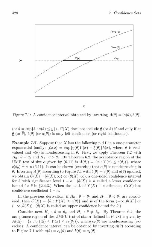
428 7. Confidence Sets
Y
θ
C(x) Y=y
Y=a
Y=b
(θ)
(θ)
Figure 7.1: A confidence interval obtained by inverting A(θ) = [a(θ), b(θ)]
(or θ = supθ : a(θ) ≤ y). C(X) does not include θ (or θ) if and only if atθ (or θ), b(θ) (or a(θ)) is only left-continuous (or right-continuous).
Example 7.7. Suppose that X has the following p.d.f. in a one-parameterexponential family: fθ(x) = expη(θ)Y (x) − ξ(θ)h(x), where θ is real-valued and η(θ) is nondecreasing in θ. First, we apply Theorem 7.2 withH0 : θ = θ0 and H1 : θ > θ0. By Theorem 6.2, the acceptance region of theUMP test of size α given by (6.11) is A(θ0) = x : Y (x) ≤ c(θ0), wherec(θ0) = c in (6.11). It can be shown (exercise) that c(θ) is nondecreasing inθ. Inverting A(θ) according to Figure 7.1 with b(θ) = c(θ) and a(θ) ignored,we obtain C(X) = [θ(X),∞) or (θ(X),∞), a one-sided confidence intervalfor θ with significance level 1 − α. (θ(X) is a called a lower confidencebound for θ in §2.4.3.) When the c.d.f. of Y (X) is continuous, C(X) hasconfidence coefficient 1 − α.
In the previous derivation, if H0 : θ = θ0 and H1 : θ < θ0 are consid-ered, then C(X) = θ : Y (X) ≥ c(θ) and is of the form (−∞, θ(X)] or(−∞, θ(X)). (θ(X) is called an upper confidence bound for θ.)
Consider next H0 : θ = θ0 and H1 : θ = θ0. By Theorem 6.4, theacceptance region of the UMPU test of size α defined in (6.28) is given byA(θ0) = x : c1(θ0) ≤ Y (x) ≤ c2(θ0), where ci(θ) are nondecreasing (ex-ercise). A confidence interval can be obtained by inverting A(θ) accordingto Figure 7.1 with a(θ) = c1(θ) and b(θ) = c2(θ).
7.1. Construction of Confidence Sets 429
Let us consider a specific example in which X1, ..., Xn are i.i.d. binaryrandom variables with p = P (Xi = 1). Note that Y (X) =
∑ni=1 Xi.
Suppose that we need a lower confidence bound for p so that we considerH0 : p = p0 and H1 : p > p0. From Example 6.2, the acceptance region ofa UMP test of size α ∈ (0, 1) is A(p0) = y : y ≤ m(p0), where m(p0) isan integer between 0 and n such that
n∑j=m(p0)+1
(n
j
)pj0(1 − p0)n−j ≤ α <
n∑j=m(p0)
(n
j
)pj0(1 − p0)n−j .
Thus, m(p) is an integer-valued, nondecreasing step-function of p. Define
p = infp : m(p) ≥ y = inf
⎧⎨⎩p :n∑
j=y
(n
j
)pj(1 − p)n−j ≥ α
⎫⎬⎭ . (7.5)
Then a level 1−α confidence interval for p is (p, 1] (exercise). One can com-pare this confidence interval with the one obtained by applying Theorem7.1 (exercise). See also Example 7.16.
Example 7.8. Suppose that X has the following p.d.f. in a multiparam-eter exponential family: fθ,ϕ(x) = exp θY (x) + U(x)ϕτ − ζ(θ, ϕ). ByTheorem 6.4, the acceptance region of a UMPU test of size α for testingH0 : θ = θ0 versus H1 : θ > θ0 or H0 : θ = θ0 versus H1 : θ = θ0 is
A(θ0) = (y, u) : y ≤ c2(u, θ0)
orA(θ0) = (y, u) : c1(u, θ0) ≤ y ≤ c2(u, θ0),
where ci(u, θ), i = 1, 2, are nondecreasing functions of θ. Confidence inter-vals for θ can then be obtained by inverting A(θ) according to Figure 7.1with b(θ) = c2(u, θ) and a(θ) = c1(u, θ) or a(θ) ≡ −∞, for any observed u.
Consider more specifically the case where X1 and X2 are independentlydistributed as the Poisson distributions P (λ1) and P (λ2), respectively, andwe need a lower confidence bound for the ratio ρ = λ2/λ1. From Example6.11, a UMPU test of size α for testing H0 : ρ = ρ0 versus H1 : ρ > ρ0has the acceptance region A(ρ0) = (y, u) : y ≤ c(u, ρ0), where c(u, ρ0) isdetermined by the conditional distribution of Y = X2 given U = X1+X2 =u. Since the conditional distribution of Y given U = u is the binomialdistribution Bi(ρ/(1 + ρ), u), we can use the result in Example 7.7, i.e.,c(u, ρ) is the same as m(p) in Example 7.7 with n = u and p = ρ/(1 + ρ).Then a level 1 − α lower confidence bound for p is p given by (7.5) withn = u. Since ρ = p/(1 − p) is a strictly increasing function of p, a level1 − α lower confidence bound for ρ is p/(1 − p).
430 7. Confidence Sets
Example 7.9. Consider the normal linear model X = Nn(βZτ , σ2In) andthe problem of constructing a confidence set for θ = βLτ , where L is ans × p matrix of rank s and all rows of L are in R(Z). It follows from thediscussion in §6.3.2 and Exercise 63 in §6.6 that a nonrandomized UMPItest of size α for H0 : θ = θ0 versus H1 : θ = θ0 has the acceptance region
A(θ0) = X : W (X, θ0) ≤ cα,
where cα is the (1 − α)th quantile of the F-distribution Fs,n−r,
W (X, θ) =[‖X − β(θ)Zτ‖2 − ‖X − βZτ‖2]/s
‖X − βZτ‖2/(n− r),
r is the rank of Z, r ≥ s, β is the LSE of β and, for each fixed θ, β(θ) is asolution of
‖X − β(θ)Zτ‖2 = minβ:βLτ=θ
‖X − βZτ‖2.
Inverting A(θ), we obtain the following confidence set for θ with confidencecoefficient 1−α: C(X) = θ : W (X, θ) ≤ cα, which is the interior and theboundary of an ellipsoid in Rs.
The last example concerns inverting the acceptance regions of tests ina nonparametric problem.
Example 7.10. Consider the problem in Example 7.6. We now derive aconfidence interval for θ by inverting the acceptance regions of the signedrank tests given by (6.79). Note that testing whether the c.d.f. of Xi issymmetric about θ is equivalent to testing whether the c.d.f. of Xi − θ issymmetric about 0. Let ci’s be given by (6.79), W be given by (6.78),and, for each θ, let Ro
+(θ) be the vector of ordered components of R+(θ)described in Example 7.6. A level 1 − α confidence set for θ is
C(X) = θ : c1 ≤ W (Ro+(θ)) ≤ c2.
The region C(X) can be computed numerically for any observed X. Fromthe discussion in Example 7.6, W (Ro
+(θ)) is a pivotal quantity and, there-fore, C(X) is the same as the confidence set obtained by using a pivotalquantity.
7.1.3 The Bayesian approach
In Bayesian analysis, analogues to confidence sets are called credible sets.Consider a sample X from a population in a parametric family indexed by
7.1. Construction of Confidence Sets 431
θ ∈ Θ ⊂ Rk and dominated by a σ-finite measure. Let fθ(x) be the p.d.f.of X and π(θ) be a prior p.d.f. w.r.t. a σ-finite measure λ on (Θ,BΘ). Let
px(θ) = fθ(x)π(θ)/m(x)
be the posterior p.d.f. w.r.t. λ, where x is the observed X and m(x) =∫Θ fθ(x)π(θ)dλ. For any α ∈ (0, 1), a level 1 − α credible set for θ is anyC ∈ BΘ with
Pθ|x(θ ∈ C) =∫C
px(θ)dλ ≥ 1 − α. (7.6)
A level 1 − α highest posterior density (HPD) credible set for θ is definedto be the event
C(x) = θ : px(θ) ≥ cα, (7.7)
where cα is chosen so that∫C(x) px(θ)dλ ≥ 1 − α. When px(θ) has a
continuous c.d.f., we can replace ≥ in (7.6) and (7.7) by =. An HPDcredible set is often an interval with the shortest length among all credibleintervals of the same level (Exercise 30).
The Bayesian credible sets and the confidence sets we have discussedso far are very different in terms of their meanings and interpretations,although sometimes they look similar. In a credible set, x is fixed andθ is considered random and the probability statement in (7.6) is w.r.t.the posterior probability Pθ|x. On the other hand, in a confidence setθ is nonrandom (although unknown) but X is considered random, andthe significance level is w.r.t. P (θ ∈ C(X)), the probability related to thedistribution of X. The set C(X) in (7.7) is not necessarily a confidence setwith significance level 1 − α.
When π(θ) is constant, which is usually an improper prior, the HPDcredible set C(x) in (7.7) is related to the idea of maximizing likelihood (anon-Bayesian approach introduced in §4.4; see also §7.3.2), since px(θ) =fθ(x)/m(x) is proportional to fθ(x) = (θ), the likelihood function. In sucha case C(X) may be a confidence set with significance level 1 − α.
Example 7.11. Let X1, ..., Xn be i.i.d. as N(θ, σ2) with an unknown θ ∈ Rand a known σ2. Let π(θ) be the p.d.f. of N(µ0, σ
20) with known µ0 and
σ20 . Then, px(θ) is the p.d.f. of N(µ∗(x), c2) (Example 2.25), where µ∗(x)
and c2 are given by (2.28), and the HPD credible set in (7.7) is
C(x) =θ : e−[θ−µ∗(x)]2/(2c2) ≥ cα
√2πc
=
θ : |θ − µ∗(x)| ≤
√2c[− log(cα
√2πc)]1/2
.
Let Φ be the standard normal c.d.f. The quantity√
2c[− log(cα√
2πc)]1/2
must be cΦ−1(1 − α/2), since it is chosen so that Pθ|x(C(x)) = 1 − α and
432 7. Confidence Sets
Pθ|x = N(µ∗(x), c2). Therefore,
C(x) = [µ∗(x) − cΦ−1(1 − α/2), µ∗(x) + cΦ−1(1 − α/2)].
If we let σ20 = ∞, which is equivalent to taking the Lebesgue measure as
the (improper) prior, then µ∗(x) = x, c2 = σ2/n, and
C(x) = [ x− σΦ−1(1 − α/2)/√n, x + σΦ−1(1 − α/2)/
√n ],
which looks the same as the classical confidence interval for θ with confi-dence coefficient 1−α (Example 2.31). Although the Bayesian credible setcoincides with the classical confidence interval, which is frequently the casewhen a noninformative prior is used, their interpretations are still different.
More details about Bayesian credible sets can be found, for example, inBerger (1985, §4.3).
7.1.4 Prediction sets
In some problems the quantity of interest is the future (or unobserved) valueof a random variable ξ. An inference procedure about a random quantityinstead of an unknown nonrandom parameter is called prediction. If thedistribution of ξ is known, then a level 1−α prediction set for ξ is any eventC satisfying Pξ(ξ ∈ C) ≥ 1 − α. In applications, however, the distributionof ξ is usually unknown.
Suppose that the distribution of ξ is related to the distribution ofa sample X from which prediction will be made. For instance, X =(X1, ..., Xn) is the observed sample and ξ = Xn+1 is to be predicted, whereX1, ..., Xn, Xn+1 are i.i.d. random variables. A set C(X) depending onlyon the sample X is said to be a level 1 − α prediction set for ξ if
infP∈P
P(ξ ∈ C(X)
)≥ 1 − α,
where P is the joint distribution of ξ and X and P contains all possible P .Note that prediction sets are very similar and closely related to confi-
dence sets. Hence, some methods for constructing confidence sets can beapplied to obtained prediction sets. For example, if (X, ξ) is a pivotalquantity in the sense that its distribution does not depend on P , then aprediction set can be obtained by inverting c1 ≤ (X, ξ) ≤ c2. The follow-ing example illustrates this idea.
Example 7.12. Many prediction problems encountered in practice can beformulated as follows. The variable ξ to be predicted is related to a vector-valued covariate ζ (called predictor) according to E(ξ|ζ) = βζτ , where β
7.1. Construction of Confidence Sets 433
is a p-vector of unknown parameters. Suppose that at ζ = Zi, we observeξ = Xi, i = 1, ..., n, and Xi’s are independent. The Zi’s are either fixedor random observations (in the latter case all probabilities given in thefollowing discussion are conditional probabilities, given Z1, ..., Zn). Basedon (X1, Z1), ..., (Xn, Zn), we would like to construct a prediction set for thevalue of ξ = X0 when ζ = Z0 ∈ R(Z), where Zτ = (Zτ
1 , ..., Zτn).
Assume further that X0, X1, ..., Xn are independently normal with acommon variance, i.e., X = (X1, ..., Xn) = Nn(βZτ , σ2In) follows a normallinear model and is independent of X0 = N(βZτ
0 , σ2). Let β be the LSE of
β, σ2 = ‖X − βZτ‖2/(n − r), and ‖Z0‖2Z = Z0(ZτZ)−Zτ
0 , where r is therank of Z. Then
(X,X0) =X0 − βZτ
0
σ√
1 + ‖Z0‖2Z
has the t-distribution tn−r and, therefore, is a pivotal quantity. This isbecause X0 and βZτ
0 are independently normal,
E(X0 − βZτ0 ) = 0, Var(X0 − βZτ
0 ) = σ2(1 + ‖Z0‖2Z),
(n − r)σ2 has the chi-square distribution χ2n−r, and X0, βZτ
0 , and σ2 areindependent (Theorem 3.8). A level 1−α prediction interval for X0 is then[
βZτ0 − tn−r,α/2σ
√1 + ‖Z0‖2
Z , βZτ0 + tn−r,α/2σ
√1 + ‖Z0‖2
Z
], (7.8)
where tn−r,α is the (1 − α)th quantile of the t-distribution tn−r.To compare prediction sets with confidence sets, let us consider a con-
fidence interval for E(X0) = βZτ0 . Using the pivotal quantity
(X,βZτ0 ) =
βZτ0 − βZτ
0
σ‖Z0‖Z,
we obtain the following confidence interval for βZτ0 with confidence coeffi-
cient 1 − α:[βZτ
0 − tn−r,α/2σ‖Z0‖Z , βZτ0 + tn−r,α/2σ‖Z0‖Z
]. (7.9)
Since a random variable is more variable than its average (an unknownparameter), the prediction interval (7.8) is much longer than the confidenceinterval (7.9), although each of them covers the quantity of interest withprobability 1 − α. In fact, when ‖Z0‖2
Z → 0 as n → ∞, the length of theconfidence interval (7.9) tends to 0 a.s., whereas the length of the predictioninterval (7.8) tends to a positive constant a.s.
Because of the similarity between confidence sets and prediction sets,in the rest of this chapter we do not discuss prediction sets in detail. Someexamples are given in Exercises 21 and 22.
434 7. Confidence Sets
7.2 Properties of Confidence Sets
In this section we study some properties of confidence sets and introduceseveral criteria for comparing confidence sets.
7.2.1 Lengths of confidence intervals
For confidence intervals of a real-valued θ with the same confidence coef-ficient, an apparent measure of their performance is the interval length.Shorter confidence intervals are preferred, since they are more informative.In most problems, however, shortest-length confidence intervals do not ex-ist. A common approach is to consider a reasonable class of confidenceintervals (with the same confidence coefficient) and then find a confidenceinterval with the shortest length within the class.
When confidence intervals are constructed by using pivotal quantitiesor by inverting acceptance regions of tests, choosing a reasonable class ofconfidence intervals amounts to selecting good pivotal quantities or tests.Functions of sufficient statistics should be used, when sufficient statisticsexist. In many problems pivotal quantities or tests are related to somepoint estimators of θ. For example, in a location family problem (Example7.1), a confidence interval for θ = µ is often of the form [θ− c, θ+ c], whereθ is an estimator of θ and c is a constant. In such a case a more accurateestimator of θ should intuitively result in a better confidence interval. Forinstance, when X1, ..., Xn are i.i.d. N(µ, 1), it can be shown (exercise) thatthe interval [X − c1, X + c1] is better than the interval [X1 − c2, X1 + c2] interms of their lengths, where ci’s are chosen so that these confidence inter-vals have confidence coefficient 1 − α. However, we cannot have the sameconclusion when Xi’s are from the Cauchy distribution C(µ, 1) (exercise).The following is another example.
Example 7.13. Let X1, ..., Xn be i.i.d. from the uniform distributionU(0, θ) with an unknown θ > 0. A confidence interval for θ of the form[b−1X(n), a
−1X(n)] is derived in Example 7.2, where a and b are constantschosen so that this confidence interval has confidence coefficient 1−α. An-other confidence interval obtained by applying Proposition 7.1 with T = Xis of the form [b−1
1 X, a−11 X], where X = (
∏ni=1 Xi)1/n. We now argue that
when n is large enough, the former has a shorter length than the latter.Note that
√n(X − θ)/θ →d N(0, 1). Thus,
P
((1 + d√
n
)−1X ≤θ≤
(1 + c√
n
)−1X
)= P
(c√n≤ X−θ
θ ≤ d√n
)→ 1−α
for some constants c and d. This means that a1 ≈ 1+c/√n, b1 ≈ 1+d/
√n,
and the length of [b−11 X, a−1
1 X] converges to 0 a.s. at the rate n−1/2. On
7.2. Properties of Confidence Sets 435
the other hand,
P((
1 + dn
)−1X(n) ≤θ≤
(1 + c
n
)−1X(n)
)= P
(cn ≤ X(n)−θ
θ ≤ dn
)→ 1 − α
for some constants c and d, since n(X(n)−θ)/θ has a known limiting distri-bution (Example 2.34). This means that the length of [b−1X(n), a
−1X(n)]converges to 0 a.s. at the rate n−1 and, therefore, [b−1X(n), a
−1X(n)] isshorter than [b−1
1 X, a−11 X] for sufficiently large n a.s.
Similarly, one can show that the confidence interval based on the pivotalquantity X/θ is not as good as [b−1X(n), a
−1X(n)] in terms of their lengths.Thus, it is reasonable to consider the class of confidence intervals of the
form [b−1X(n), a−1X(n)] subject to P (b−1X(n) ≤ θ ≤ a−1X(n)) = 1 − α.
The shortest-length interval within this class can be derived as follows.Note that X(n)/θ has the Lebesgue p.d.f. nxn−1I(0,1)(x). Hence
1 − α = P (b−1X(n) ≤ θ ≤ a−1X(n)) =∫ b
a
nxn−1dx = bn − an.
This implies that 1 ≥ b > a ≥ 0 and dadb = ( b
a )n−1. Since the length of theinterval [b−1X(n), a
−1X(n)] is ψ(a, b) = X(n)(a−1 − b−1),
dψ
db= X(n)
(1b2
− 1a2
da
db
)= X(n)
an+1 − bn+1
b2an+1 < 0.
Hence the minimum occurs at b = 1 (a = α1/n). This shows that theshortest-length interval is [X(n), α
−1/nX(n)].
As Example 7.13 indicates, whence a reasonable class of confidence in-tervals is chosen (using some good estimators, pivotal quantities, or tests),we may find the shortest-length confidence interval within the class by di-rectly analyzing the lengths of the intervals. For a large class of problems,the following result can be used.
Theorem 7.3. Let θ be a real-valued parameter and T (X) be a real-valuedstatistic.(i) Let U(X) be a positive statistic. Suppose that (T − θ)/U is a pivotalquantity having a Lebesgue p.d.f. f that is unimodal at x0 ∈ R in the sensethat f(x) is nondecreasing for x ≤ x0 and f(x) is nonincreasing for x ≥ x0.Consider the following class of confidence intervals for θ:
C =
[T − bU, T − aU ] :
∫ b
a
f(x)dx = 1 − α
. (7.10)
If [T − b∗U, T − a∗U ] ∈ C, f(a∗) = f(b∗) > 0, and a∗ ≤ x0 ≤ b∗, then theinterval [T − b∗U, T − a∗U ] has the shortest length within C.
436 7. Confidence Sets
(ii) Suppose that T > 0, θ > 0, T/θ is a pivotal quantity having a Lebesguep.d.f. f , and that x2f(x) is unimodal at x0. Consider the following class ofconfidence intervals for θ:
C =
[b−1T, a−1T ] :
∫ b
a
f(x)dx = 1 − α
. (7.11)
If [b−1∗ T, a−1
∗ T ] ∈ C, a2∗f(a∗) = b2∗f(b∗) > 0, and a∗ ≤ x0 ≤ b∗, then the
interval [b−1∗ T, a−1
∗ T ] has the shortest length within C.Proof. We prove (i) only. The proof of (ii) is left as an exercise. Note thatthe length of an interval in C is (b − a)U . Thus, it suffices to show that ifa < b and b − a < b∗ − a∗, then
∫ b
af(x)dx < 1 − α. Assume that a < b,
b− a < b∗ − a∗, and a ≤ a∗ (the proof for a > a∗ is similar).If b ≤ a∗, then a ≤ b ≤ a∗ ≤ x0 and∫ b
a
f(x)dx ≤ f(a∗)(b− a) < f(a∗)(b∗ − a∗) ≤∫ b∗
a∗f(x)dx = 1 − α,
where the first inequality follows from the unimodality of f , the strict in-equality follows from b− a < b∗ − a∗ and f(a∗) > 0, and the last inequalityfollows from the unimodality of f and the fact that f(a∗) = f(b∗).
If b > a∗, then a ≤ a∗ < b < b∗. By the unimodality of f ,∫ a∗
a
f(x)dx ≤ f(a∗)(a∗ − a) and∫ b∗
b
f(x)dx ≥ f(b∗)(b∗ − b).
Then ∫ b
a
f(x)dx =∫ b∗
a∗f(x)dx +
∫ a∗
a
f(x)dx−∫ b∗
b
f(x)dx
= 1 − α +∫ a∗
a
f(x)dx−∫ b∗
b
f(x)dx
≤ 1 − α + f(a∗)(a∗ − a) − f(b∗)(b∗ − b)= 1 − α + f(a∗)[(a∗ − a) − (b∗ − b)]= 1 − α + f(a∗)[(b− a) − (b∗ − a∗)]< 1 − α.
Example 7.14. Let X1, ..., Xn be i.i.d. from N(µ, σ2) with unknown µ andσ2. Confidence intervals for θ = µ using the pivotal quantity
√n(X−µ)/S
form the class C in (7.10) with f being the p.d.f. of the t-distribution tn−1,which is unimodal at x0 = 0. Hence, we can apply Theorem 7.3(i). Since fis symmetric about 0, f(a∗) = f(b∗) implies a∗ = −b∗ (exercise). Therefore,the equal-tail confidence interval[
X − tn−1,α/2S/√n, X + tn−1,α/2S/
√n]
(7.12)
7.2. Properties of Confidence Sets 437
has the shortest length within C.If θ = µ and σ2 is known, then we can replace S by σ and f by the
standard normal p.d.f. (i.e., use the pivotal quantity√n(X − µ)/σ instead
of√n(X − µ)/S). The resulting confidence interval is[
X − Φ−1(1 − α/2)σ/√n, X + Φ−1(1 − α/2)σ/
√n], (7.13)
which is the shortest interval of the form [X − b, X − a] with confidencecoefficient 1−α. The difference in length of the intervals in (7.12) and (7.13)is a random variable so that we cannot tell which one is better in general.But the expected length of the interval (7.13) is always shorter than that ofthe interval (7.12) (exercise). This again shows the importance of pickingthe right pivotal quantity.
Consider next confidence intervals for θ = σ2 using the pivotal quantity(n − 1)S2/σ2, which form the class C in (7.11) with f being the p.d.f. ofthe chi-square distribution χ2
n−1. Note that x2f(x) is unimodal, but notsymmetric. By Theorem 7.3(ii), the shortest-length interval within C is
[ b−1∗ (n− 1)S2, a−1
∗ (n− 1)S2 ], (7.14)
where a∗ and b∗ are solutions of a2∗f(a∗) = b2∗f(b∗) and
∫ b∗a∗
f(x)dx = 1−α.Numerical values of a∗ and b∗ can be obtained (Tate and Klett, 1959). Notethat this interval is not equal-tail.
If θ = σ2 and µ is known, then a better pivotal quantity is T/σ2, whereT =
∑ni=1(Xi−µ)2. One can show (exercise) that if we replace (n−1)S2 by
T and f by the p.d.f. of the chi-square distribution χ2n, then the resulting
interval has shorter expected length than that of the interval in (7.14).Suppose that we need a confidence interval for θ = σ when µ is unknown.
Consider the class of confidence intervals[b−1/2√n− 1S, a−1/2√n− 1S
]with
∫ b
af(x)dx = 1 − α. The shortest-length interval, however, is not the
one with the endpoints equal to the square roots of the endpoints of theinterval (7.14) (Exercise 26(c)).
Note that Theorem 7.3(ii) cannot be applied to obtain the result inExample 7.13 unless n = 1, since the p.d.f. of X(n)/θ is strictly increasingwhen n > 1. A result similar to Theorem 7.3, which can be applied toExample 7.13, is given in Exercise 28.
The result in Theorem 7.3 can also be applied to justify the idea of HPDcredible sets in Bayesian analysis (Exercise 30).
If a confidence interval has the shortest length within a class of con-fidence intervals, then its expected length is also the shortest within the
438 7. Confidence Sets
same class, provided that its expected length is finite. In a problem wherea shortest-length confidence interval does not exist, we may have to usethe expected length as the criterion in comparing confidence intervals. Forinstance, the expected length of the interval in (7.13) is always shorter thanthat of the interval in (7.12), whereas the probability that the interval in(7.12) is shorter than the interval in (7.13) is positive for any fixed n. An-other example is the interval [X(n), α
−1/nX(n)] in Example 7.13. Althoughwe are not able to say that this interval has the shortest length among allconfidence intervals for θ with confidence coefficient 1 − α, we can showthat it has the shortest expected length, using the results in Theorems 7.4and 7.6 (§7.2.2).
For one-sided confidence intervals (confidence bounds) of a real-valuedθ, their lengths may be infinity. We can use the distance between theconfidence bound and θ as a criterion in comparing confidence bounds,which is equivalent to comparing the tightness of confidence bounds. Letθj , j = 1, 2, be two lower confidence bounds for θ with the same confidencecoefficient. If θ1 − θ ≥ θ2 − θ is always true, then θ1 ≥ θ2 and θ1 is tighter(more informative) than θ2. Again, since θj are random, we may have toconsider E(θj − θ) and choose θ1 if E(θ1) ≥ E(θ2). As a specific example,consider i.i.d. X1, ..., Xn from N(θ, 1). If we use the pivotal quantity X−µ,then θ1 = X −Φ−1(1−α)/
√n. If we use the pivotal quantity X1 −µ, then
θ2 = X1 − Φ−1(1 − α). Clearly E(θ1) ≥ E(θ2). Although θ1 is intuitivelypreferred, θ1 < θ2 with a positive probability for any fixed n > 1.
Some ideas discussed previously can be extended to the comparison ofconfidence sets for multivariate θ. For bounded confidence sets in Rk, forexample, we may consider their volumes (Lebesgue measures). However, inmultivariate cases it is difficult to compare the volumes of confidence setswith different shapes. Some results about expected volumes of confidencesets are given in Theorem 7.6.
7.2.2 UMA and UMAU confidence sets
For a confidence set obtained by inverting the acceptance regions of someUMP or UMPU tests, it is expected that the confidence set inherits someoptimality property.
Definition 7.2. Let θ ∈ Θ be an unknown parameter and Θ′ be a subsetof Θ that does not contain the true parameter value θ. A confidence setC(X) for θ with confidence coefficient 1−α is said to be Θ′-uniformly mostaccurate (UMA) if and only if for any other confidence set C1(X) withconfidence coefficient 1 − α,
P(θ′ ∈ C(X)
)≤ P
(θ′ ∈ C1(X)
)for all θ′ ∈ Θ′. (7.15)
7.2. Properties of Confidence Sets 439
C(X) is UMA if Θ′ = θc (the set containing all false values).
The probabilities in (7.15) are probabilities of covering false values. In-tuitively, confidence sets with small probabilities of covering wrong param-eter values are preferred. The reason why we sometimes need to considera Θ′ different from θc is that for some confidence sets such as one-sidedconfidence intervals, we do not need to worry about the probabilities ofcovering some false values. For example, if we consider a lower confidencebound for a real-valued θ, we are asserting that θ is larger than a certainvalue and we only need to worry about covering values of θ that are toosmall. Thus, Θ′ = θ′ ∈ Θ : θ′ < θ. A similar discussion leads to theconsideration of Θ′ = θ′ ∈ Θ : θ′ > θ for upper confidence bounds.
Theorem 7.4. Let C(X) be a confidence set for θ obtained by inverting theacceptance regions of nonrandomized tests Tθ0 for testing H0 : θ = θ0 versusH1 : θ ∈ Θθ0 . Suppose that for each θ0, Tθ0 is UMP of size α. Then C(X)is Θ′-UMA with confidence coefficient 1 − α, where Θ′ = θ′ : θ ∈ Θθ′.Proof. The fact that C(X) has confidence coefficient 1 − α follows fromTheorem 7.2. Let C1(X) be another confidence set with confidence coef-ficient 1 − α. By Proposition 7.2, the test T1θ0(X) = 1 − IA1(θ0)(X) withA1(θ0) = x : θ0 ∈ C1(x) has size α for testing H0 : θ = θ0 versusH1 : θ ∈ Θθ0 . For any θ′ ∈ Θ′,
P(θ′ ∈ C(X)
)= P
(Tθ′(X) = 0
)= 1 − P
(Tθ′(X) = 1
)≤ 1 − P
(T1θ′(X) = 1
)= P
(X ∈ A1(θ′)
)= P
(θ′ ∈ C1(X)
),
where the second equality follows from the fact that Tθ′ is nonrandomizedand the inequality follows from the fact that Tθ′ is UMP.
Theorem 7.4 can be applied to construct UMA confidence bounds inproblems where the population is in a one-parameter parametric familywith monotone likelihood ratio so that UMP tests exist (Theorem 6.2).It can also be applied to a few cases to construct two-sided UMA confi-dence intervals. For example, the confidence interval [X(n), α
−1/nX(n)] inExample 7.13 is UMA (exercise).
As we discussed in §6.2, in many problems there are UMPU tests butnot UMP tests. This leads to the following definition.
Definition 7.3. Let C(X) be a confidence set for θ with confidence coeffi-cient 1−α and Θ′ be a subset of Θ that does not contain the true parameter
440 7. Confidence Sets
value θ.(i) If P (θ′ ∈ C(X)) ≤ 1 − α for all θ′ ∈ Θ′, then C(X) is said to be Θ′-unbiased (unbiased if Θ′ = θc).(ii) If C(X) is Θ′-unbiased and (7.15) holds for any other Θ′-unbiasedconfidence set C1(X) with confidence coefficient 1 − α, then C(X) is saidto be Θ′-uniformly most accurate unbiased (UMAU). C(X) is UMAU ifΘ′ = θc.
Theorem 7.5. Let C(X) be a confidence set for θ obtained by invertingthe acceptance regions of nonrandomized tests Tθ0 for testing H0 : θ = θ0versus H1 : θ ∈ Θθ0 . If Tθ0 is unbiased of size α for each θ0, then C(X) isΘ′-unbiased with confidence coefficient 1− α, where Θ′ = θ′ : θ ∈ Θθ′; ifTθ0 is also UMPU for each θ0, then C(X) is Θ′-UMAU.
The proof of Theorem 7.5 is very similar to that of Theorem 7.4.It follows from Theorem 7.5 and the results in §6.2 that the confidence
intervals in (7.12), (7.13) and (7.14) are UMAU, since they can be obtainedby inverting acceptance regions of UMPU tests (Exercise 14).
Example 7.15. Consider the normal linear model in Example 7.9 and theparameter θ = βlτ , where l ∈ R(Z). From §6.2.3, the nonrandomized testwith acceptance region
A(θ0) =X : βlτ − θ0 > tn−r,α
√l(ZτZ)−lτSSR/(n− r)
is UMPU with size α for testing H0 : θ = θ0 versus H1 : θ < θ0, where β isthe LSE of β and tn−r,α is the (1−α)th quantile of the t-distribution tn−r.Inverting A(θ) we obtain the following Θ′-UMAU upper confidence boundwith confidence coefficient 1 − α and Θ′ = (θ,∞):
θ = βlτ − tn−r,α
√l(ZτZ)−lτSSR/(n− r).
A UMAU confidence interval for θ can be similarly obtained.If θ = βLτ with L described in Example 7.9 and s > 1, then θ is
multivariate. It can be shown that the confidence set derived in Example7.9 is unbiased (exercise), but it may not be UMAU.
The volume of a confidence set C(X) for θ ∈ Rk when X = x is definedto be vol(C(x)) =
∫C(x) dθ
′ (if it is well defined), which is the Lebesguemeasure of the set C(x). In particular, if θ is real-valued and C(X) =[θ(X), θ(X)] is a confidence interval, then vol(C(x)) is simply the length ofC(x). The next result reveals a relationship between the expected volume(length) and the probability of covering a false value of a confidence set(interval).
7.2. Properties of Confidence Sets 441
Theorem 7.6 (Pratt’s theorem). Let X be a sample from P and C(X)be a confidence set for θ ∈ Rk. Suppose that for each x in the range of X,vol(C(x)) =
∫C(x) dθ
′ is well defined. Then the expected volume of C(X)is
E[vol(C(X))] =∫θ =θ′
P(θ′ ∈ C(X)
)dθ′. (7.16)
Proof. By Fubini’s theorem,
E[vol(C(X))] =∫
vol(C(X))dP
=∫ [∫
C(x)dθ′
]dP (x)
=∫ ∫
θ′∈C(x)dθ′dP (x)
=∫ [∫
θ′∈C(x)dP (x)
]dθ′
=∫
P(θ′ ∈ C(X)
)dθ′
=∫θ =θ′
P(θ′ ∈ C(X)
)dθ′.
This proves the result.
It follows from Theorem 7.6 that if C(X) is UMA (or UMAU) with con-fidence coefficient 1 − α, then it has the smallest expected volume amongall confidence sets (or all unbiased confidence sets) with confidence coef-ficient 1 − α. For example, the confidence intervals (7.13) in Example7.14 (when σ2 is known) and [X(n), α
−1/nX(n)] in Example 7.13 have theshortest expected length among all confidence intervals with confidence co-efficient 1 − α; the confidence intervals (7.12) and (7.14) have the shortestexpected lengths among all unbiased confidence intervals with confidencecoefficient 1 − α.
7.2.3 Randomized confidence sets
Applications of Theorems 7.4 and 7.5 require that C(X) be obtained byinverting acceptance regions of nonrandomized tests. Thus, these resultscannot be directly applied to discrete problems. In fact, in discrete prob-lems inverting acceptance regions of randomized tests may not lead to aconfidence set with a given confidence coefficient. Note that randomizationis used in hypothesis testing to obtain tests with a given size. Thus, the
442 7. Confidence Sets
same idea can be applied to confidence sets, i.e., we may consider random-ized confidence sets.
Suppose that we invert acceptance regions of randomized tests Tθ0 thatreject H0 : θ = θ0 with probability Tθ0(x) when X = x. Let U be a randomvariable that is independent of X and has the uniform distribution U(0, 1).Then the test Tθ0(X,U) = I(U,1](Tθ0) has the same power function as Tθ0
and is “nonrandomized” if U is viewed as part of the sample. Let
AU (θ0) = (x, U) : U ≥ Tθ0(x)be the acceptance region of Tθ0(X,U). If Tθ0 has size α for all θ0, theninverting AU (θ) we obtain a confidence set
C(X,U) = θ : (X,U) ∈ AU (θ)having confidence coefficient 1 − α, since
P(θ ∈ C(X,U)
)= E
[P(U ≥ Tθ(X)|X
)]= E
[1 − Tθ(X)
].
If Tθ0 is UMP (or UMPU) for each θ0, then C(X,U) is UMA (or UMAU).However, C(X,U) is a randomized confidence set since it is still randomwhen we observe X = x.
When Tθ0 is integer-valued, we can use the method in the followingexample to derive C(X,U).
Example 7.16. Let X1, ..., Xn be i.i.d. binary random variables with p =P (Xi = 1). The confidence coefficient of (p, 1] may not be 1 − α, where pis given by (7.5).
From Example 6.2 and the previous discussion, a randomized UMP testfor testing H0 : p = p0 versus H1 : p > p0 can be constructed based onY =
∑ni=1 Xi and U , a random variable that is independent of Y and has
the uniform distribution U(0, 1). Since Y is integer-valued and U ∈ (0, 1),W = Y + U is equivalent to (Y,U). Hence, we can also construct a UMPtest based on W . It can be shown (exercise) that W has the followingLebesgue p.d.f.:
fp(w) =(
n
[w]
)p[w](1 − p)n−[w]I(0,n+1)(w), (7.17)
where [w] is the integer part of w, and that the family fp : p ∈ (0, 1) hasmonotone likelihood ratio in W . It follows from Theorem 6.2 that the testTp0(Y,U) = I(c(p0),n+1)(W ) is UMP of size α for testing H0 : p = p0 versusH1 : p > p0, where α =
∫ n+1c(p0)
fp0(w)dw. Inverting the acceptance regions
of Tp(Y,U), a lower confidence bound p1
for p is the solution of∫ n+1
Y +U
(n
[w]
)p[w](1 − p)n−[w]dw = α
7.2. Properties of Confidence Sets 443
(p1
= 0 if Y = 0 and U < α). This lower confidence bound has confidencecoefficient 1 − α and is Θ′-UMA with Θ′ = (0, p).
Using a randomized confidence set, we can achieve the purpose of ob-taining a confidence set with a given confidence coefficient as well as someoptimality properties such as UMA, UMAU, or shortest expected length.On the other hand, randomization may not be desired in practical problems.
7.2.4 Invariant confidence sets
Let C(X) be a confidence set for θ and g be a one-to-one transformation.The invariance principle requires that C(x) change in a specified way whenx is transformed to g(x).
Definition 7.4. Let G be a group of one-to-one transformations of X suchthat P is invariant (Definition 6.5). Let θ = θ(P ) be a parameter withrange Θ. Assume that g(θ) = θ(Pg(X)) is well defined for any g, i.e., g isa transformation on Θ induced by g (g = g given in Definition 6.5 if P isindexed by θ).(i) A confidence set C(X) is invariant under G if and only if θ ∈ C(x) isequivalent to g(θ) ∈ C(g(x)) for every x in the range of X, θ ∈ Θ, andg ∈ G.(ii) C(X) is Θ′-uniformly most accurate invariant (UMAI) with confidencecoefficient 1−α if and only if C(X) is invariant with confidence coefficient1 − α and (7.15) holds for any other invariant confidence set C1(X) withconfidence coefficient 1 − α. C(X) is UMAI if Θ′ = θc.
Example 7.17. Consider the confidence intervals in Example 7.14. LetG = gr,c : r > 0, c ∈ R with gr,c(x) = (rx1 + c, ..., rxn + c). Let θ = µ.Then gr,c(µ, σ2) = (rµ + c, r2σ2) and g(µ) = rµ + c. Clearly, confidenceinterval (7.12) is invariant under G.
When σ2 is known, the family P is not invariant under G and we considerG1 = g1,c : c ∈ R. Then both confidence intervals (7.12) and (7.13) areinvariant under G1.
Suppose now that θ = σ2. For gr,c ∈ G, g(σ2) = r2σ2. Hence confidenceinterval (7.14) is invariant under G.
If a confidence set C(X) is UMA and invariant, then it is UMAI. IfC(X) is UMAU and invariant, it is not so obvious whether it is UMAI,since a UMAI confidence set (if it exists) is not necessarily unbiased. Thefollowing result may be used to construct a UMAI confidence set.
Theorem 7.7. Suppose that for each θ0 ∈ Θ, A(θ0) is the acceptance
444 7. Confidence Sets
region of a nonrandomized UMPI test of size α for H0 : θ = θ0 versus H1 :θ ∈ Θθ0 under Gθ0 and that for any θ0 and g ∈ Gθ0 , g, the transformationon Θ induced by g, is well defined. If C(X) = θ : x ∈ A(θ) is invariantunder G, the smallest group containing ∪θ∈ΘGθ, then it is Θ′-UMAI withconfidence coefficient 1 − α, where Θ′ = θ′ : θ ∈ Θθ′.
The proofs of Theorem 7.7 and the following result are given as exercises.
Proposition 7.3. Let P be a parametric family indexed by θ and G bea group of transformations such that g is well defined by Pg(θ) = Pg(X).Suppose that, for any θ, θ′ ∈ Θ, there is a g ∈ G such that g(θ) = θ′. Then,for any invariant confidence set C(X), P (θ ∈ C(X)) is a constant.
Example 7.18. Let X1, ..., Xn be i.i.d. from N(µ, σ2) with unknown µand σ2. Consider the problem of setting a lower confidence bound forθ = µ/σ and G = gr : r > 0 with gr(x) = rx. From Example 6.17, anonrandomized UMPI test of size α for H0 : θ = θ0 versus H1 : θ > θ0 hasthe acceptance region A(θ0) = x : t(x) ≤ c(θ0), where t(X) =
√nX/S
and c(θ) is the (1−α)th quantile of the noncentral t-distribution tn−1(√nθ).
Applying Theorem 7.7 with Gθ0 = G for all θ0, one can show (exercise) thatthe solution of
∫ ∞t(x) fθ(u)du = α is a Θ′-UMAI lower confidence bound for
θ with confidence coefficient 1 − α, where fθ is the Lebesgue p.d.f. of thenoncentral t-distribution tn−1(
√nθ) and Θ′ = (−∞, θ).
Example 7.19. Consider again the confidence intervals in Example 7.14.In Example 7.17, confidence interval (7.12) is shown to be invariant underG = gr,c : r > 0, c ∈ R with gr,c(x) = (rx1 +c, ..., rxn+c). Although con-fidence interval (7.12) is UMAU, it is not obvious whether it is UMAI. Thisinterval can be obtained by inverting A(µ0) = x : |X−µ0| ≤ t1−α/2S/
√n,
which is the acceptance region of a nonrandomized test UMP among unbi-ased and invariant tests of size α for H0 : µ = µ0 versus H1 : µ = µ0, underGµ0 = hr,µ0 : r > 0 with hr,µ0(x) = (r(x1 − µ0) + µ0, ..., r(xn − µ0) + µ0)(exercise). Note that the testing problem H0 : µ = µ0 versus H1 : µ = µ0 isnot invariant under G. Since G is the smallest group containing ∪µ0∈RGµ0
(exercise), by Theorem 7.7, interval (7.12) is UMA among unbiased andinvariant confidence intervals with confidence coefficient 1 − α, under G.
Using similar arguments one can show (exercise) that confidence inter-vals (7.13) and (7.14) are UMA among unbiased and invariant confidenceintervals with confidence coefficient 1−α, under G1 (in Example 7.17) andG, respectively.
When UMPI tests are randomized, one can construct randomized UMAIconfidence sets, using the techniques introduced in Theorem 7.7 and §7.2.3.
7.3. Asymptotic Confidence Sets 445
7.3 Asymptotic Confidence Sets
In some problems, especially in nonparametric problems, it is difficult tofind a reasonable confidence set with a given confidence coefficient or sig-nificance level 1−α. A common approach is to find a confidence set whoseconfidence coefficient or significance level is nearly 1 − α when the samplesize n is large. According to Definition 2.4, a confidence set C(X) for θ hasasymptotic significance level 1− α if lim infn P (θ ∈ C(X)) ≥ 1− α for anyP ∈ P. If limn→∞ P (θ ∈ C(X)) = 1−α for any P ∈ P, then C(X) is a 1−αasymptotically correct confidence set. Note that asymptotic correctness isnot the same as having limiting confidence coefficient 1−α (Definition 2.4).
7.3.1 Asymptotically pivotal quantities
A known Borel function of (X, θ), n(X, θ), is said to be asymptoticallypivotal if the limiting distribution of n(X, θ) does not depend on P . Likea pivotal quantity in constructing confidence sets (§7.1.1) with a given con-fidence coefficient or significance level, an asymptotically pivotal quantitycan be used in constructing asymptotically correct confidence sets.
Most asymptotically pivotal quantities are of the form (θn − θ)V −1/2n ,
where θn is an estimator of θ that is asymptotically normal, i.e.,
(θn − θ)V −1/2n →d Nk(0, Ik), (7.18)
and Vn is an estimator of the asymptotic covariance matrix Vn and is consis-tent according to Definition 5.4. The resulting 1−α asymptotically correctconfidence sets are of the form
C(X) = θ : ‖(θn − θ)V −1/2n ‖2 ≤ χ2
k,α, (7.19)
where χ2k,α is the (1 − α)th quantile of the chi-square distribution χ2
k. If θis real-valued (k = 1), then C(X) in (7.19) is a 1−α asymptotically correctconfidence interval. When k > 1, C(X) in (7.19) is an ellipsoid.
Example 7.20 (Functions of means). Suppose that X1, ..., Xn are i.i.d.random vectors having a c.d.f. F on Rd and that the unknown parameterof interest is θ = g(µ), where µ = E(X1) and g is a known differentiablefunction from Rd to Rk, k ≤ d. From the CLT (Theorem 1.12) and theresult in §5.5.1, (7.18) holds with θn = g(X) and Vn given by (5.102). Thus,C(X) in (7.19) is a 1 − α asymptotically correct confidence set for θ.
Example 7.21 (Statistical functionals). Suppose that X1, ..., Xn are i.i.d.random vectors having a c.d.f. F on Rd and that the unknown parameterof interest is θ = T(F ), where T is a k-vector-valued functional. Let Fn be
446 7. Confidence Sets
the empirical c.d.f. defined by (5.1) and θn = T(Fn). Suppose that eachcomponent of T is ∞-Hadamard differentiable with an influence functionsatisfying (5.33) and that the conditions in Theorem 5.15 hold. Then, byTheorems 5.5 and 5.15 and the discussions in §5.2.1, (7.18) holds withVn given by (5.105) and C(X) in (7.19) is a 1 − α asymptotically correctconfidence set for θ.
Example 7.22 (Linear models). Consider linear model (3.25): X = βZτ +ε, where ε has i.i.d. components with mean 0 and variance σ2. Assume thatZ is of full rank and that the conditions in Theorem 3.12 hold. It followsfrom Theorem 1.9(iii) and Theorem 3.12 that (7.18) holds with θn = β andVn = (n − p)−1SSR(ZτZ)−1 (see §5.5.1). Thus, a 1 − α asymptoticallycorrect confidence set for β is
C(X) = β : (β − β)(ZτZ)(β − β)τ ≤ χ2p,αSSR/(n− p).
Note that this confidence set is different from the one in Example 7.9 derivedunder the normality assumption on ε.
The problems in the previous three examples are nonparametric. Themethod of using asymptotically pivotal quantities can also be applied toparametric problems. Note that in a parametric problem where the un-known parameter θ is multivariate, a confidence set for θ with a givenconfidence coefficient may be difficult or impossible to obtain.
Typically, in a given problem there exist many different asymptoticallypivotal quantities that lead to different 1 − α asymptotically correct con-fidence sets for θ. Intuitively, if two asymptotic confidence sets are con-structed using (7.18) with two different estimators, θ1n and θ2n, and if θ1n
is asymptotically more efficient than θ2n (§4.5.1), then the confidence setbased on θ1n should be better than the one based on θ2n in some sense.This is formally stated in the following result.
Proposition 7.4. Let Cj(X), j = 1, 2, be the confidence sets given in(7.19) with θn = θjn and Vn = Vjn, j = 1, 2, respectively. Suppose that foreach j, (7.18) holds for θjn and Vjn is consistent for Vjn, the asymptoticcovariance matrix of θjn. If Det(V1n) < Det(V2n) for sufficiently large n,where Det(A) is the determinant of A, then
P(vol(C1(X)) < vol(C2(X))
)→ 1.
Proof. The result follows from the consistency of Vjn and the fact thatthe volume of the ellipsoid C(X) defined by (7.19) is equal to
vol(C(X)) =πk/2(χ2
p,α)k/2[Det(Vn)]1/2
Γ(1 + k/2).
7.3. Asymptotic Confidence Sets 447
If θ1n is asymptotically more efficient than θ2n (§4.5.1), then Det(V1n) ≤Det(V2n). Hence, Proposition 7.4 indicates that a more efficient estimatorof θ results in a better confidence set of the form (7.19) in terms of volume.If θn is asymptotically efficient (optimal in the sense of having the smallestasymptotic covariance matrix; see Definition 4.4), then the confidence setC(X) in (7.19) is asymptotically optimal (in terms of volume) among theconfidence sets of the form (7.19).
Asymptotically correct confidence sets for θ can also be constructed byinverting acceptance regions of asymptotic tests for testing H0 : θ = θ0versus some H1. If asymptotic tests are constructed using asymptoticallypivotal quantities (see §6.4.2, §6.4.3, and §6.5.4), the resulting confidencesets are almost the same as those based on asymptotically pivotal quantities.
7.3.2 Confidence sets based on likelihoods
As we discussed in §7.3.1, a 1−α asymptotically correct confidence set forθ is asymptotically optimal in some sense if it is based on a point estimatorθn which is asymptotically efficient. In parametric problems, it is shownin §4.5 that MLE’s or RLE’s of θ are asymptotically efficient. Thus, inthis section we study more closely the asymptotic confidence sets based onMLE’s and RLE’s or, more generally, based on likelihoods.
Consider first the case where P = Pθ : θ ∈ Θ is a parametric familydominated by a σ-finite measure, where Θ ⊂ Rk. Let (θ) be the likelihoodfunction based on the observation X = x. The acceptance region of the LRtest defined in §6.4.1 with Θ0 = θ0 is
A(θ0) = x : (θ0) ≥ e−cα/2(θ),
where (θ) = supθ∈Θ (θ) and cα is a constant related to the significancelevel α. Under the conditions of Theorem 6.5, if cα is chosen to be χ2
k,α,the (1 − α)th quantile of the chi-square distribution χ2
k, then
C(X) = θ ∈ Θ : (θ) ≥ e−cα/2(θ) (7.20)
is a 1 − α asymptotically correct confidence set. Note that this confidenceset and the one given by (7.19) are generally different.
In many cases (θ) is a convex function of θ and, therefore, the setdefined by (7.20) is a bounded set in Rk; in particular, C(X) in (7.20) is abounded interval when k = 1.
Let θ = (ϑ, ϕ), where ϑ is r × 1. Then a 1 − α asymptotically correctconfidence set for ϑ is also given by (7.20) with (θ) replaced by (ϑ, ϕ) =supϕ (ϑ, ϕ) and cα replaced by χ2
r,α, the (1−α)th quantile of the chi-squaredistribution χ2
r.
448 7. Confidence Sets
In §6.4.2 we discussed two asymptotic tests closely related to the LRtest: Wald’s test and Rao’s score test. When Θ0 = θ0, Wald’s test hasacceptance region
A(θ0) = x : (θ − θ0)In(θ)(θ − θ0)τ ≤ χ2k,α, (7.21)
where θ is an MLE or RLE of θ and In(θ) is the Fisher information matrixbased on X. The confidence set obtained by inverting A(θ) in (7.21) is thesame as that in (7.19) with Vn = [In(θ)]−1, which is consistent for [In(θ)]−1,the asymptotic covariance matrix of θ (e.g., Theorem 4.17 or 4.18).
When Θ0 = θ0, Rao’s score test has the acceptance region
A(θ0) = x : sn(θ0)[In(θ0)]−1[sn(θ0)]τ ≤ χ2k,α, (7.22)
where sn(θ) = ∂ log (θ)/∂θ. The confidence set obtained by inverting A(θ)in (7.22) is also 1−α asymptotically correct, but is generally different fromthe previous two confidence sets. To illustrate these likelihood-based con-fidence sets and their differences, we consider the following two examples.
Example 7.23. Let X1, ..., Xn be i.i.d. binary random variables with p =P (Xi = 1). Since confidence sets for p with a given confidence coefficientare usually randomized (§7.2.3), asymptotically correct confidence sets maybe considered when n is large.
The likelihood ratio for testing H0 : p = p0 versus H1 : p = p0 is
λ(Y ) = pY0 (1 − p0)n−Y /pY (1 − p)n−Y ,
where Y =∑n
i=1 Xi and p = Y/n is the MLE of p. The confidence set(7.20) is then equal to
C1(X) = p : pY (1 − p)n−Y ≥ e−cα/2pY (1 − p)n−Y .
When 0 < Y < n, pY (1 − p)n−Y is strictly convex and equals 0 if p = 0 or1 and, hence, C1(X) = [p, p] with 0 < p < p < 1. When Y = 0, (1 − p)n isstrictly decreasing and, therefore, C1(X) = (0, p] with 0 < p < 1. Similarly,when Y = n, C1(X) = [p, 1) with 0 < p < 1.
The confidence set obtained by inverting acceptance regions of Wald’stests is simply
C2(X) = [ p− Φ−1(1 − α/2)√
p(1 − p)/n, p + Φ−1(1 − α/2)√
p(1 − p)/n ],
since In(p) = n/[p(1 − p)] and (χ21,α)1/2 = Φ−1(1 − α/2). Note that
sn(p) =Y
p− n− Y
1 − p=
Y − pn
p(1 − p)
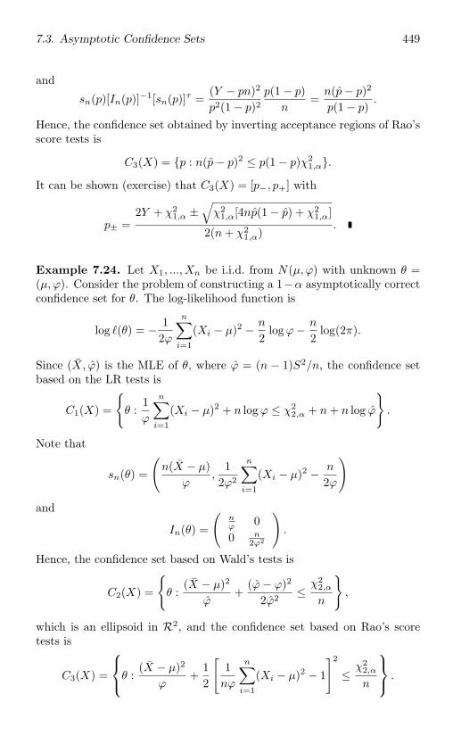
7.3. Asymptotic Confidence Sets 449
and
sn(p)[In(p)]−1[sn(p)]τ =(Y − pn)2
p2(1 − p)2p(1 − p)
n=
n(p− p)2
p(1 − p).
Hence, the confidence set obtained by inverting acceptance regions of Rao’sscore tests is
C3(X) = p : n(p− p)2 ≤ p(1 − p)χ21,α.
It can be shown (exercise) that C3(X) = [p−, p+] with
p± =2Y + χ2
1,α ±√χ2
1,α[4np(1 − p) + χ21,α]
2(n + χ21,α)
.
Example 7.24. Let X1, ..., Xn be i.i.d. from N(µ, ϕ) with unknown θ =(µ, ϕ). Consider the problem of constructing a 1−α asymptotically correctconfidence set for θ. The log-likelihood function is
log (θ) = − 12ϕ
n∑i=1
(Xi − µ)2 − n
2logϕ− n
2log(2π).
Since (X, ϕ) is the MLE of θ, where ϕ = (n − 1)S2/n, the confidence setbased on the LR tests is
C1(X) =
θ :
1ϕ
n∑i=1
(Xi − µ)2 + n logϕ ≤ χ22,α + n + n log ϕ
.
Note that
sn(θ) =
(n(X − µ)
ϕ,
12ϕ2
n∑i=1
(Xi − µ)2 − n
2ϕ
)and
In(θ) =
(nϕ 00 n
2ϕ2
).
Hence, the confidence set based on Wald’s tests is
C2(X) =
θ :
(X − µ)2
ϕ+
(ϕ− ϕ)2
2ϕ2 ≤χ2
2,α
n
,
which is an ellipsoid in R2, and the confidence set based on Rao’s scoretests is
C3(X) =
⎧⎨⎩θ :(X − µ)2
ϕ+
12
[1nϕ
n∑i=1
(Xi − µ)2 − 1
]2
≤χ2
2,α
n
⎫⎬⎭ .
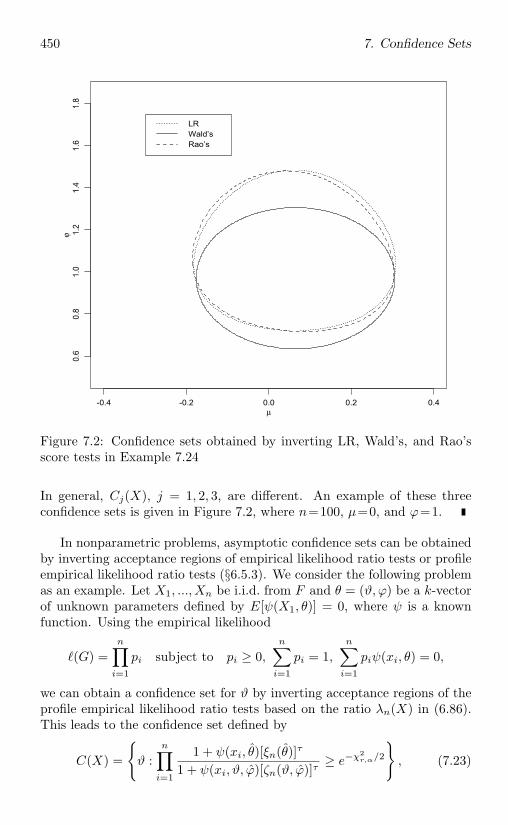
450 7. Confidence Sets
-0.4 -0.2 0.0 0.2 0.4
0.6
0.8
1.0
1.2
1.4
1.6
1.8
µ
ϕ
LRWald’sRao’s
Figure 7.2: Confidence sets obtained by inverting LR, Wald’s, and Rao’sscore tests in Example 7.24
In general, Cj(X), j = 1, 2, 3, are different. An example of these threeconfidence sets is given in Figure 7.2, where n=100, µ=0, and ϕ=1.
In nonparametric problems, asymptotic confidence sets can be obtainedby inverting acceptance regions of empirical likelihood ratio tests or profileempirical likelihood ratio tests (§6.5.3). We consider the following problemas an example. Let X1, ..., Xn be i.i.d. from F and θ = (ϑ, ϕ) be a k-vectorof unknown parameters defined by E[ψ(X1, θ)] = 0, where ψ is a knownfunction. Using the empirical likelihood
(G) =n∏
i=1
pi subject to pi ≥ 0,n∑
i=1
pi = 1,n∑
i=1
piψ(xi, θ) = 0,
we can obtain a confidence set for ϑ by inverting acceptance regions of theprofile empirical likelihood ratio tests based on the ratio λn(X) in (6.86).This leads to the confidence set defined by
C(X) =
ϑ :
n∏i=1
1 + ψ(xi, θ)[ξn(θ)]τ
1 + ψ(xi, ϑ, ϕ)[ζn(ϑ, ϕ)]τ≥ e−χ2
r,α/2
, (7.23)
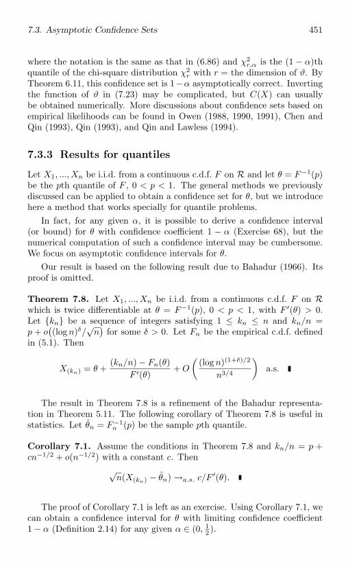
7.3. Asymptotic Confidence Sets 451
where the notation is the same as that in (6.86) and χ2r,α is the (1 − α)th
quantile of the chi-square distribution χ2r with r = the dimension of ϑ. By
Theorem 6.11, this confidence set is 1−α asymptotically correct. Invertingthe function of ϑ in (7.23) may be complicated, but C(X) can usuallybe obtained numerically. More discussions about confidence sets based onempirical likelihoods can be found in Owen (1988, 1990, 1991), Chen andQin (1993), Qin (1993), and Qin and Lawless (1994).
7.3.3 Results for quantiles
Let X1, ..., Xn be i.i.d. from a continuous c.d.f. F on R and let θ = F−1(p)be the pth quantile of F , 0 < p < 1. The general methods we previouslydiscussed can be applied to obtain a confidence set for θ, but we introducehere a method that works specially for quantile problems.
In fact, for any given α, it is possible to derive a confidence interval(or bound) for θ with confidence coefficient 1 − α (Exercise 68), but thenumerical computation of such a confidence interval may be cumbersome.We focus on asymptotic confidence intervals for θ.
Our result is based on the following result due to Bahadur (1966). Itsproof is omitted.
Theorem 7.8. Let X1, ..., Xn be i.i.d. from a continuous c.d.f. F on Rwhich is twice differentiable at θ = F−1(p), 0 < p < 1, with F ′(θ) > 0.Let kn be a sequence of integers satisfying 1 ≤ kn ≤ n and kn/n =p + o
((log n)δ/
√n)
for some δ > 0. Let Fn be the empirical c.d.f. definedin (5.1). Then
X(kn) = θ +(kn/n) − Fn(θ)
F ′(θ)+ O
((log n)(1+δ)/2
n3/4
)a.s.
The result in Theorem 7.8 is a refinement of the Bahadur representa-tion in Theorem 5.11. The following corollary of Theorem 7.8 is useful instatistics. Let θn = F−1
n (p) be the sample pth quantile.
Corollary 7.1. Assume the conditions in Theorem 7.8 and kn/n = p +cn−1/2 + o(n−1/2) with a constant c. Then
√n(X(kn) − θn) →a.s. c/F
′(θ).
The proof of Corollary 7.1 is left as an exercise. Using Corollary 7.1, wecan obtain a confidence interval for θ with limiting confidence coefficient1 − α (Definition 2.14) for any given α ∈ (0, 1
2 ).
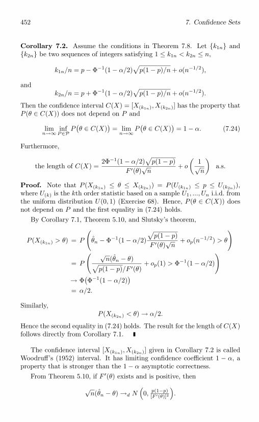
452 7. Confidence Sets
Corollary 7.2. Assume the conditions in Theorem 7.8. Let k1n andk2n be two sequences of integers satisfying 1 ≤ k1n < k2n ≤ n,
k1n/n = p− Φ−1(1 − α/2)√
p(1 − p)/n + o(n−1/2),
andk2n/n = p + Φ−1(1 − α/2)
√p(1 − p)/n + o(n−1/2).
Then the confidence interval C(X) = [X(k1n), X(k2n)] has the property thatP (θ ∈ C(X)) does not depend on P and
limn→∞
infP∈P
P(θ ∈ C(X)
)= lim
n→∞P(θ ∈ C(X)
)= 1 − α. (7.24)
Furthermore,
the length of C(X) =2Φ−1(1 − α/2)
√p(1 − p)
F ′(θ)√n
+ o
(1√n
)a.s.
Proof. Note that P (X(k1n) ≤ θ ≤ X(k2n)) = P (U(k1n) ≤ p ≤ U(k2n)),where U(k) is the kth order statistic based on a sample U1, ..., Un i.i.d. fromthe uniform distribution U(0, 1) (Exercise 68). Hence, P (θ ∈ C(X)) doesnot depend on P and the first equality in (7.24) holds.
By Corollary 7.1, Theorem 5.10, and Slutsky’s theorem,
P (X(k1n) > θ) = P
(θn − Φ−1(1 − α/2)
√p(1 − p)
F ′(θ)√n
+ op(n−1/2) > θ
)
= P
( √n(θn − θ)√
p(1 − p)/F ′(θ)+ op(1) > Φ−1(1 − α/2)
)→ Φ
(Φ−1(1 − α/2)
)= α/2.
Similarly,P (X(k2n) < θ) → α/2.
Hence the second equality in (7.24) holds. The result for the length of C(X)follows directly from Corollary 7.1.
The confidence interval [X(k1n), X(k2n)] given in Corollary 7.2 is calledWoodruff’s (1952) interval. It has limiting confidence coefficient 1 − α, aproperty that is stronger than the 1 − α asymptotic correctness.
From Theorem 5.10, if F ′(θ) exists and is positive, then
√n(θn − θ) →d N
(0, p(1−p)
[F ′(θ)]2
).
7.4. Bootstrap Confidence Sets 453
If the derivative F ′(θ) has a consistent estimator dn obtained using somemethod such as one of those introduced in §5.1.3, then (7.18) holds withVn = p(1 − p)/d2
n and the method introduced in §7.3.1 can be applied toderive the following 1 − α asymptotically correct confidence interval:
C(X) =[θn − Φ−1(1 − α/2)
√p(1−p)
dn√n
, θn + Φ−1(1 − α/2)√
p(1−p)
dn√n
].
The length of C(X) is asymptotically almost the same as Woodruff’s in-terval. However, C(X) depends on the estimated derivative dn and it isusually difficult to obtain a precise estimator dn.
7.4 Bootstrap Confidence Sets
In this section we study how to use the bootstrap method introduced in§5.5.3 to construct asymptotically correct confidence sets. There are twomain advantages of using the bootstrap method. First, as we can see fromprevious sections, constructing confidence sets having a given confidencecoefficient or being asymptotically correct requires some theoretical deriva-tions. The bootstrap method replaces these derivations by some routinecomputations. Second, confidence intervals (especially one-sided confidenceintervals) constructed using the bootstrap method may be asymptoticallymore accurate than those asymptotic confidence sets discussed in §7.3.
We use the notation in §5.5.3. Let X = (X1, ..., Xn) be a sample from P .We focus on the case where Xi’s are i.i.d. so that P is specified by a c.d.f. Fon Rd, although some results discussed here can be extended to non-i.i.d.cases. Also, we assume that F is estimated by the empirical c.d.f. Fn definedin (5.1) (which means that no assumption is imposed on F and the problemis nonparametric) so that P in §5.5.3 is the population corresponding to Fn.A bootstrap sample X∗ = (X∗
1 , ..., X∗n) is obtained from P , i.e., X∗
i ’s arei.i.d. from Fn. Some other bootstrap sampling procedures are described inExercises 72 and 75-77. Let θ be a parameter of interest, θn be an estimatorof θ, and θ∗n be the bootstrap analogue of θn, i.e., θ∗n is the same as θn exceptthat X is replaced by the bootstrap sample X∗.
7.4.1 Construction of bootstrap confidence intervals
We now introduce several different ways of constructing bootstrap confi-dence intervals for a real-valued θ. Some ideas can be extended to theconstruction of bootstrap confidence sets for multivariate θ. We mainlyconsider lower confidence bounds. Upper confidence bounds and two-sidedconfidence intervals can be similarly obtained.
454 7. Confidence Sets
The bootstrap percentile
DefineKB(x) = P∗(θ∗n ≤ x), (7.25)
where P∗ denotes the distribution of X∗ conditional on X. For a givenα ∈ (0, 1
2 ), the bootstrap percentile method (Efron, 1981) gives the followinglower confidence bound for θ:
θBP = K−1B (α). (7.26)
The name percentile comes from the fact that K−1B (α) is a percentile of the
bootstrap distribution KB in (7.25).For most cases, the computation of θBP requires numerical approxima-
tions such as the Monte Carlo approximation described in §5.5.3.We now provide a justification of the bootstrap percentile method that
allows us to see what assumptions are required for a good performance of abootstrap percentile confidence set. Suppose that there exists an increasingtransformation φn(x) such that
P(φn − φn(θ) ≤ x
)= Ψ(x) (7.27)
holds for all possible F (including F = Fn), where φn = φn(θn) and Ψis a c.d.f. that is continuous, increasing, and symmetric about 0. WhenΨ = Φ, the standard normal distribution, the function φn is called the nor-malizing and variance stabilizing transformation. If φn and Ψ in (7.27) canbe derived, then the following lower confidence bound for θ has confidencecoefficient 1 − α:
θE = φ−1n (φn + zα),
where zα = Ψ−1(α).We now show that θBP = θE and, therefore, we can still use this lower
confidence bound without deriving φn and Ψ. Let wn = φn(θBP ) − φn.From the fact that assumption (7.27) holds when F is replaced by Fn,
Ψ(wn) = P∗(φ∗n − φn ≤ wn) = P∗(θ∗n ≤ θBP ) = α,
where φ∗n = φn(θ∗n) and the last equality follows from the definition of θBP
and the assumption on Ψ. Hence wn = zα = Ψ−1(α) and
θBP = φ−1n (φn + zα) = θE .
Thus, the bootstrap percentile lower confidence bound θBP has confi-dence coefficient 1 − α for all n if assumption (7.27) holds exactly for alln. If assumption (7.27) holds approximately for large n, then θBP is 1− αasymptotically correct (see Theorem 7.9 in §7.4.2) and its performance de-pends on how good the approximation is.
7.4. Bootstrap Confidence Sets 455
The bootstrap bias-corrected percentile
Efron (1981) considered the following assumption that is more general thanassumption (7.27):
P(φn − φn(θ) + z0 ≤ x
)= Ψ(x), (7.28)
where φn and Ψ are the same as those in (7.27) and z0 is a constant thatmay depend on F and n. When z0 = 0, (7.28) reduces to (7.27). SinceΨ(0) = 1
2 , z0 is a kind of “bias” of φn. If φn, z0, and Ψ in (7.28) canbe derived, then a lower confidence bound for θ with confidence coefficient1 − α is
θE = φ−1n (φn + zα + z0).
Applying assumption (7.28) to F = Fn, we obtain that
KB(θn) = P∗(φ∗n − φn + z0 ≤ z0) = Ψ(z0),
where KB is given in (7.25). This implies
z0 = Ψ−1(KB(θn)). (7.29)
Also from (7.28),
1 − α = Ψ(−zα)
= Ψ(φn − φn(θE) + z0
)= P∗
(φ∗n − φn ≤ φn − φn(θE)
)= P∗
(θ∗n ≤ φ−1
n (φn − zα − z0)),
which impliesφ−1n (φn − zα − z0) = K−1
B (1 − α).
Since this equation holds for any α, it implies that for 0 < x < 1,
K−1B (x) = φ−1
n
(φn + Ψ−1(x) − z0
). (7.30)
By the definition of θE and (7.30),
θE = K−1B
(Ψ(zα + 2z0)
).
Assuming that Ψ is known (e.g., Ψ = Φ) and using (7.29), Efron (1981) ob-tained the bootstrap bias-corrected (BC) percentile lower confidence boundfor θ:
θBC = K−1B
(Ψ(zα + 2Ψ−1(KB(θn))
)), (7.31)
which is a percentile of the bootstrap distribution KB . Note that θBC
reduces to θBP if KB(θn) = 12 , i.e., θn is the median of the bootstrap
456 7. Confidence Sets
distribution KB . Hence, the bootstrap BC percentile method is a bias-corrected version of the bootstrap percentile method and the bias-correctionis represented by 2Ψ−1(KB(θn)). If (7.28) holds exactly, then θBC hasconfidence coefficient 1 − α for all n. If (7.28) holds approximately, thenθBC is 1 − α asymptotically correct.
The bootstrap BC percentile method improves the bootstrap percentilemethod by taking a bias into account. This is supported by the theoreticalresult in §7.4.2. However, there are still many cases where assumption (7.28)cannot be fulfilled nicely and the bootstrap BC percentile method does notwork well. Efron (1987) proposed a bootstrap accelerated bias-corrected(BCa) percentile method (see Exercise 73) that improves the bootstrap BCpercentile method. However, applications of the bootstrap BCa percentilemethod involve some derivations that may be very complicated. See Efron(1987) and Efron and Tibshirani (1993) for details.
The hybrid bootstrap
Suppose that θn is asymptotically normal, i.e., (7.18) holds with Vn = σ2F /n.
Let Hn be the c.d.f. of√n(θn − θ) and
HB(x) = P∗(√
n(θ∗n − θn) ≤ x)
be its bootstrap estimator defined in (5.116). From the results in Theorem5.20, for any t ∈ (0, 1), H−1
B (t) − H−1n (t) →p 0. Treating the quantile of
HB as the quantile of Hn, we obtain the following hybrid bootstrap lowerconfidence bound for θ:
θHB = θn − n−1/2H−1B (1 − α). (7.32)
The bootstrap-t
Suppose that (7.18) holds with Vn = σ2F /n and σ2
F is a consistent estimatorof σ2
F . The bootstrap-t method is based on t(X, θ) =√n(θn − θ)/σF ,
which is often called a studentized “statistic”. If the distribution Gn oft(X, θ) is known (i.e., t(X, θ) is pivotal), then a confidence interval for θwith confidence coefficient 1−α can be obtained (§7.1.1). If Gn is unknown,it can be estimated by the bootstrap estimator
GB(x) = P∗(t(X∗, θn) ≤ x
),
where t(X∗, θn) =√n(θ∗n− θn)/σ∗
F and σ∗F is the bootstrap analogue of σF .
Treating the quantile of GB as the quantile of Gn, we obtain the followingbootstrap-t lower confidence bound for θ:
θBT = θn − n−1/2σF G−1B (1 − α). (7.33)
7.4. Bootstrap Confidence Sets 457
Although it is shown in §7.4.2 that θBT in (7.33) is more accurate thanθBP in (7.26), θBC in (7.31), and θHB in (7.32), the use of the bootstrap-tmethod requires a consistent variance estimator σ2
F .
7.4.2 Asymptotic correctness and accuracy
From the construction of the hybrid bootstrap and bootstrap-t confidencebounds, θHB is 1−α asymptotically correct if ∞(HB , Hn) →p 0, and θBT
is 1 − α asymptotically correct if ∞(GB , Gn) →p 0. On the other hand,the asymptotic correctness of the bootstrap percentile (with or withoutbias-correction or acceleration) confidence bounds requires slightly more.
Theorem 7.9. Suppose that ∞(HB , Hn) →p 0 and
limn→∞
ρ∞(Hn, H) = 0, (7.34)
where H is a c.d.f. on R that is continuous, strictly increasing, and symmet-ric about 0. Then θBP in (7.26) and θBC in (7.31) are 1−α asymptoticallycorrect.Proof. The result for θBP follows from
P(θBP ≤ θ
)= P
(α ≤ KB(θ)
)= P
(α ≤ HB
(√n(θ − θn)
))= P
(√n(θn − θ) ≤ −H−1
B (α))
= P(√
n(θn − θ) ≤ −H−1(α))
+ o(1)
= H(−H−1(α)
)+ o(1)
= 1 − α + o(1).
The result for θBC follows from the previous result and
z0 = Ψ−1(KB(θn))
= Ψ−1(HB(0))→p Ψ−1(H(0)
)= 0.
Theorem 7.9 can be obviously extended to the case of upper confidencebounds or two-sided confidence intervals. The result also holds for thebootstrap BCa percentile confidence intervals.
Note that H in (7.34) is not the same as Ψ in assumption (7.28). UsuallyH(x) = Φ(x/σF ) for some σF > 0, whereas Ψ = Φ. Also, condition (7.34)is much weaker than assumption (7.28), since the latter requires variancestabilizing.
It is not surprising that all bootstrap methods introduced in §7.3.1 pro-duce asymptotically correct confidence sets. To compare various bootstrap
458 7. Confidence Sets
confidence intervals and other asymptotic confidence intervals, we now con-sider the convergence rate of their coverage probability.
Definition 7.5. A confidence set C(X) for θ is said to be lth-order (asymp-totically) accurate if and only if P (θ ∈ C(X)) = 1− α+O(n−l/2), where lis a positive integer.
We now discuss the results in Hall (1988) and sketch the proofs. Con-sider the case of θ = g(µ), µ = EX1, and θn = g(X), where g is continuouslydifferentiable from Rd to R with ∇g(µ) = 0. The asymptotic variance of√n(θn − θ) is σ2
F = ∇g(µ)Var(X1)[∇g(µ)]τ and a consistent estimator ofσ2F is σ2
F = n−1n ∇g(X)S2[∇g(X)]τ , where S2 is the sample covariance ma-
trix. Let Gn be the distribution of√n(θn − θ)/σF . If Gn is known, then a
lower confidence bound for θ with confidence coefficient 1 − α is:
θE = θn − n−1/2σFG−1n (1 − α), (7.35)
which is not useful if Gn is unknown.Suppose that G−1
n (t) has the following Cornish-Fisher expansion on acompact interval:
G−1n (t) = zt +
q1(zt, F )√n
+q2(zt, F )
n+ o
(1n
), (7.36)
which is a type of an inverse of the following Edgeworth expansion:
Gn(x) = Φ(x) −[q1(x, F )√
n+
q3(x, F )n
]Φ′(x) + o
(1n
), (7.37)
where Φ and Φ′ are, respectively, the c.d.f. and p.d.f. of the standard normaldistribution, qj ’s are some functions depending on F , and zt = Φ−1(t).More details about these expansions can be found, for example, in Hall(1992). Let GB be the bootstrap estimator of Gn defined in §7.4.1. Undersome conditions (Hall, 1992), G−1
B admits expansion (7.36) with F replacedby Fn for almost all sequences X1, X2, .... Hence the bootstrap-t lowerconfidence bound in (7.33) can be written as
θBT = θn − σF√n
[z1−α +
2∑j=1
qj(z1−α, Fn)nj/2 + o
(1n
)]a.s. (7.38)
Under some moment conditions, qj(x, Fn) − qj(x, F ) = Op(n−1/2) for eachx, j = 1, 2. Then, comparing (7.35), (7.36), and (7.38), we obtain that
θBT − θE = Op(n−3/2). (7.39)
7.4. Bootstrap Confidence Sets 459
Furthermore,
P (θBT ≤ θ) = P
(θn − θ
σF /√n≤ G−1
B (1 − α))
= P
(θn − θ
σF /√n≤ z1−α +
2∑j=1
qj(z1−α, Fn)nj/2
)+ o
(1n
)
= P
(θn − θ
σF /√n≤ z1−α +
2∑j=1
qj(z1−α, F )nj/2
)
+ψ(z1−α)
n+ o
(1n
)= 1 − α +
ψ(z1−α)Φ′(z1−α)n
+ o
(1n
), (7.40)
where ψ(x) is a polynomial whose coefficients are functions of moments ofF and the last two equalities can be justified by a somewhat complicatedargument (Hall, 1992).
Result (7.40) implies that θBT is second-order accurate according toDefinition 7.5. The same can be concluded for the bootstrap-t upper con-fidence bound and the two-sided bootstrap-t confidence interval for θ.
Next, we consider the hybrid bootstrap lower confidence bound θHB
given by (7.32). Let HB be the bootstrap estimator of Hn, the distributionof
√n(θn − θ)/σF . Then H−1
B (1 − α) = σF H−1B (1 − α) and
θHB = θn − n−1/2σF H−1B (1 − α),
which can be viewed as a bootstrap approximation to
θH = θn − n−1/2σF H−1n (1 − α).
Note that θH does not have confidence coefficient 1−α, since it is obtainedby muddling up G−1
n (1 − α) and H−1n (1 − α). Similar to G−1
n , under someconditions H−1
n admits a Cornish-Fisher expansion
H−1n (t) = zt +
q1(zt, F
)√n
+q2
(zt, F
)n
+ o
(1n
)(7.41)
and H−1B admits the same expansion (7.41) with F replaced by Fn for
almost all X1, X2, .... Then
θHB = θn − σF√n
[z1−α +
2∑j=1
qj(z1−α, Fn)nj/2 + o
(1n
)]a.s. (7.42)
460 7. Confidence Sets
and, by (7.35),θHB − θE = Op(n−1), (7.43)
since q1(x, F ) and q1(x, F ) are usually different. Results (7.39) and (7.43)imply that θHB is not as close to θE as θBT . Similar to (7.40), we can showthat (Hall, 1992)
P (θHB ≤ θ) = P
(θn − θ
σF /√n≤ H−1
B (1 − α))
= P
(θn − θ
σF /√n≤ z1−α +
2∑j=1
qj(z1−α, Fn)nj/2
)+ o
(1n
)
= P
(θn − θ
σF /√n≤ z1−α +
2∑j=1
qj(z1−α, F )nj/2
)+ O
(1n
)
= 1 − α +ψ(z1−α)Φ′(z1−α)√
n+ O
(1n
), (7.44)
where ψ(x) is an even polynomial. This implies that when ψ ≡ 0, θHB isonly first-order accurate according to Definition 7.5.
The same conclusion can be drawn for the hybrid bootstrap upper confi-dence bounds. However, the two-sided hybrid bootstrap confidence interval
[ θHB , θHB ] = [ θn − n−1/2H−1B (1 − α), θn − n−1/2H−1
B (α) ]
is second-order accurate, as is the two-sided bootstrap-t confidence interval,since
P (θHB ≤ θ ≤ θHB) = P (θ ≤ θHB) − P (θ < θHB)= 1 − α + n−1/2ψ(z1−α)Φ′(z1−α)
− α− n−1/2ψ(zα)Φ′(zα) + O(n−1)= 1 − 2α + O(n−1)
by the fact that ψ and Φ′ are even functions and z1−α = −zα.For the bootstrap percentile lower confidence bound in (7.26),
θBP = K−1B (α) = θn + n−1/2H−1
B (α).
Comparing θBP with θBT and θHB , we find that the bootstrap percentilemethod muddles up not only H−1
B (1−α) and G−1B (1−α), but also H−1
B (α)and −H−1
B (1 − α). If HB is asymptotically symmetric about 0, then thebootstrap percentile method is equivalent to the hybrid bootstrap methodand, therefore, one-sided bootstrap percentile confidence intervals are only
7.4. Bootstrap Confidence Sets 461
first-order accurate and the two-sided bootstrap percentile confidence in-terval is second-order accurate.
Since θn is asymptotically normal, we can use Ψ = Φ for the bootstrapBC percentile method. Let αn = Φ(zα + 2z0). Then the bootstrap BCpercentile lower confidence bound given by (7.31) is just the αnth quantileof KB in (7.25). Using the Edgeworth expansion, we obtain that
KB(θn) = HB(0) = Φ(0) +q(0, Fn)Φ′(0)√
n+ Op
(1n
)with some function q and, therefore,
αn = α +2q(0, Fn)Φ′(zα)√
n+ Op
(1n
).
This result and the Cornish-Fisher expansion for H−1B imply
H−1B (αn) = zα +
2q(0, Fn) + q1(zα, Fn)√n
+ Op
(1n
).
Then from (7.31) and K−1B (αn) = θn + n−1/2σF H
−1B (αn),
θBC = θn +σF√n
[zα +
2q(0, Fn) + q1(zα, Fn)√n
+ Op
(1n
)]. (7.45)
Comparing (7.35) with (7.45), we conclude that
θBC − θE = Op(n−1).
It also follows from (7.45) that
P (θBC ≤ θ) = 1 − α +ψ(z1−α)Φ′(z1−α)√
n+ O
(1n
)(7.46)
with an even polynomial ψ(x). Hence θBC is first-order accurate in general.In fact,
θBC − θBP = 2q(0, Fn)σFn−1 + Op(n−3/2)
and, therefore, the bootstrap BC percentile and the bootstrap percentileconfidence intervals have the same order of accuracy. The bootstrap BCpercentile method, however, is a partial improvement over the bootstrappercentile method in the sense that the absolute value of ψ(z1−α) in (7.46)is smaller than that of ψ(z1−α) in (7.44) (see Example 7.25).
While the bootstrap BC percentile method does not improve the boot-strap percentile method in terms of accuracy order, Hall (1988) showed thatthe bootstrap BCa percentile method in Efron (1987) produces second-order
462 7. Confidence Sets
accurate one-sided and two-sided confidence intervals and that (7.39) holdswith θBT replaced by the bootstrap BCa percentile lower confidence bound.
We have considered the order of asymptotic accuracy for all bootstrapconfidence intervals introduced in §7.4.1. In summary, all two-sided con-fidence intervals are second-order accurate; the one-sided bootstrap-t andbootstrap BCa percentile confidence intervals are second-order accuratewhereas the one-sided bootstrap percentile, bootstrap BC percentile, andhybrid bootstrap confidence intervals are first-order accurate; however, thelatter three are simpler than the former two.
What is the order of accuracy of the asymptotic confidence intervalsderived in §7.3.1? The lower confidence bound derived in §7.3.1 is
θN = θn − n−1/2σF z1−α. (7.47)
From (7.42), we obtain that
θN − θHB = Op(n−1).
Hence, confidence intervals obtained using the method in §7.3.1 have thesame order of accuracy as the hybrid bootstrap confidence intervals.
Example 7.25. Suppose that d = 1 and g(x) = x. Under some condi-tions (see Hall (1992)) expansions (7.36) and (7.37) hold with q1(x, F ) =−γ(2x2 + 1)/6, q2(x, F ) = x[(x2 + 3)/4− κ(x2 − 3)/12 + 5γ2(4x2 − 1)/72],and q3(x, F ) = x[(x2 + 3)/4 + γ2(x4 + 2x2 − 3)/18 − κ(x2 − 3)/12], whereγ = E(X1 − µ)3/σ3 (skewness), κ = E(X1 − µ)4/σ4 − 3 (kurtosis), andσ2 = Var(X1). Also, expansion (7.41) holds with q1(x, F ) = γ(x2 − 1)/6and q2(x, F ) = x[κ(x2 − 3)/24 − γ2(2x2 − 5)/36].
The function ψ in (7.40) is equal to x(1+2x2)(κ−3γ2/2)/6; the functionψ in (7.44) is equal to γx2/2; and the function ψ(x) in (7.46) is equal toγ(x2 + 2)/6 (see Liu and Singh (1987)). If γ = 0, then θHB , θBC , and θNare first-order accurate. In this example, we can still compare their relativeperformances in terms of the convergence speed of the coverage probability.Let
e(θ) = P (θ ≤ θ) − (1 − α)
be the error in coverage probability for the lower confidence bound θ. Itcan be shown (exercise) that
|e(θHB)| = |e(θN )| + Cn(zα, F ) + o(n−1/2) (7.48)
and|e(θN )| = |e(θBC)| + Cn(zα, F ) + o(n−1/2), (7.49)
where Cn(x, F ) = |γ|(x2 − 1)Φ′(x)/(6√n). Assume γ = 0. When z2
α > 1,which is usually the case in practice, Cn(zα, F ) > 0 and, therefore, θBC is
7.4. Bootstrap Confidence Sets 463
better than θN , which is better than θHB . The use of θN requires a varianceestimator σ2
F , which is not required by the bootstrap BC percentile andhybrid bootstrap methods. When a variance estimator is available, we canuse the bootstrap-t lower confidence bound, which is second-order accurateeven when γ = 0.
7.4.3 High-order accurate bootstrap confidence sets
Can we obtain a confidence interval with a higher order accuracy thanthe second-order accuracy? The answer is affirmative under some condi-tions. Suppose that we construct a confidence set for θ (not necessarilyreal-valued) based on an asymptotically pivotal quantity n that admitsan Edgeworth expansion
P (n ≤ x) = Φ(x) +l∑
j=1
ηj(x)Φ′(x)nj/2 + O
(1
n(l+1)/2
),
where ηj are some polynomials whose coefficients depend on F . Then thereexist polynomials ζj such that
P
(n ≤ x−
l∑j=1
ζj(x)nj/2
)= Φ(x) + O
(1
n(l+1)/2
)(7.50)
(Hall, 1992). Let ζj be consistent estimators of ζj . Then (7.50) still holdswith ζj replaced by ζj and we can obtain an (l + 1)th-order accurate con-fidence set
C(l)EDG(X) =
θ : n ≤ z1−α −
l∑j=1
ζj(z1−α)nj/2
. (7.51)
To use C(l)EDG(X), we need to derive the polynomials ζj ’s, which is com-
plicated. The bootstrap method can be used to obtain confidence sets asaccurate as C
(l)EDG(X) without requiring the theoretical derivation of ζj ’s
but requiring some extra extensive computations.
The bootstrap prepivoting and bootstrap inverting
The hybrid bootstrap and the bootstrap-t are based on the bootstrap dis-tribution estimators for
√n(θn−θ) and
√n(θn−θ)/σF , respectively. Beran
(1987) argued that the reason why the bootstrap-t is better than the hybridbootstrap is that
√n(θn − θ)/σF is more pivotal than
√n(θn − θ) in the
464 7. Confidence Sets
sense that the distribution of√n(θn − θ)/σF is less dependent on the un-
known F . The bootstrap-t method, however, requires a variance estimatorσ2F . Beran (1987) suggested the following method called bootstrap prepivot-
ing. Let (0)n be a random function (such as
√n(θn− θ) or
√n(θn− θ)/σF )
used to construct a confidence set for θ ∈ Rk, H(0)n be the distribution of
(0)n , and let H
(0)B be the bootstrap estimator of H(0)
n . Define
(1)n = H
(0)B ((0)
n ). (7.52)
If H(0)n is continuous and if we replace H
(0)B in (7.52) by H
(0)n , then (1)
n
has the uniform distribution U(0, 1). Hence, it is expected that (1)n is
more pivotal than (0)n . Let H
(1)B be the bootstrap estimator of H(1)
n , thedistribution of (1)
n . Then (2)n = H
(1)B ((1)
n ) is more pivotal than (1)n .
In general, let H(j)n be the distribution of (j)
n and H(j)B be the bootstrap
estimator of H(j)n , j = 0, 1, 2, .... Then we can use the following confidence
sets for θ:
C(j)PREB(X) = θ : (j)
n ≤ (H(j)B )−1(1 − α), j = 0, 1, 2, .... (7.53)
Note that for each j, C(j)PREB(X) is a hybrid bootstrap confidence set based
on (j)n . Since (j+1)
n is more pivotal than (j)n , we obtain a sequence of
confidence sets with increasing accuracies. Beran (1987) showed that ifthe distribution of
√n(θn − θ) has a two-term Edgeworth expansion, then
the one-sided confidence interval C(1)PREB(X) based on (0)
n =√n(θn − θ)
is second-order accurate, and the two-sided confidence interval C(1)PREB(X)
based on (0)n =
√n|θn − θ| is third-order accurate. Hence, bootstrap
prepivoting with one iteration improves the hybrid bootstrap method. It isexpected that the one-sided confidence interval C(2)
PREB(X) based on (0)n =√
n(θn − θ) is third-order accurate, i.e., it is better than the one-sidedbootstrap-t or bootstrap BCa percentile confidence interval. More detaileddiscussion can be found in Beran (1987).
It seems that, using this iterative method, we can start with a (0)n
and obtain a bootstrap confidence set that is as accurate as we want itto be. However, more computations are required for higher stage boot-strapping and, therefore, the practical implementation of this method isvery hard or even impossible, with current computational ability. We ex-plain this with the computation of C(1)
PREB(X) based on (0)n = (X,F ).
Suppose that we use the Monte Carlo approximation. Let X∗1b, ..., X
∗nb
be i.i.d. samples from Fn, b = 1, ..., B1. Then H(0)B is approximated by
H(0,B1)B , the empirical distribution of (0)∗
nb : b = 1, ..., B1, where (0)∗nb =
(X∗1b, ..., X
∗nb, Fn). For each b, let F ∗
nb be the empirical distribution of
7.4. Bootstrap Confidence Sets 465
X∗1b, ..., X
∗nb, X∗∗
1bj , ..., X∗∗nbj be i.i.d. samples from F ∗
nb, j = 1, ..., B2, H∗b
be the empirical c.d.f. of n(X∗∗1bj , ..., X
∗∗nbj , F
∗nb), j = 1, ..., B2, and z∗b =
H∗b ((0)∗
nb ). Then H(1)B can be approximated by H
(1,B1B2)B , the empirical
distribution of z∗b , b = 1, ..., B1, and the confidence set C(1)PREB(X) can
be approximated byθ : (X,F ) ≤ (H(0,B1)
B )−1((H(1,B1B2)B )−1(1 − α)
).
The second-stage bootstrap sampling is nested in the first-stage bootstrapsampling. Thus the total number of bootstrap data sets we need is B1B2,which is why this method is also called the double bootstrap. If eachstage requires 1,000 bootstrap replicates, then the total number of boot-strap replicates is 1,000,000! Similarly, to compute C
(j)PREB(X) we need
(1, 000)j+1 bootstrap replicates, j = 2, 3, ..., which limits the application ofthe bootstrap prepivoting method.
A very similar method, bootstrap inverting, is given in Hall (1992). In-stead of using (7.53), we define
C(j)INV B(X) = θ : (j)
n ≤ (H(j)B )−1(1 − α), j = 0, 1, 2, . . . ,
where(j)
n = (j−1)n − (H(j−1)
B )−1(1 − α), j = 1, 2, . . . ,
and H(j)B is the bootstrap estimator of the distribution of (j)
n . For eachj ≥ 1, C(j)
INV B(X), C(j)PREB(X) in (7.53), and C
(j)EDG(X) in (7.51) have the
same order of accuracy. Thus, the analytic derivation of ζj ’s in the Edge-worth expansion (7.50) can be accomplished by bootstrap prepivoting orbootstrap inverting. Bootstrap prepivoting and bootstrap inverting requirethe same amount of computation and both of them are special cases of ageneral iterative bootstrap introduced by Hall and Martin (1988).
Bootstrap calibrating
Suppose that we want a confidence set C(X) with confidence coefficient1 − α, which is called the nominal level. The basic idea of bootstrap cali-brating is to improve C(X) by adjusting its nominal level. Let πn be theactual coverage probability of C(X). The value of πn can be estimated bya bootstrap estimator πn. If we find that πn is far from 1 − α, then weconstruct a confidence set C1(X) with nominal level 1− α so that the cov-erage probability of C1(X) is closer to 1−α than πn. Bootstrap calibratingcan be used iteratively as follows: estimate the true coverage probabilityof C1(X); if the difference between 1−α and the estimated coverage prob-ability of C1(X) is still large, we can adjust the nominal level again andconstruct a new calibrated confidence set C2(X).
466 7. Confidence Sets
The key for bootstrap calibrating is how to determine the new nominallevel 1−α in each step. We now discuss the method suggested by Loh (1987,1991) in the case where the initial confidence sets are obtained by using themethod in §7.3.1. Consider first the lower confidence bound θN defined in(7.47). The coverage probability πn = P (θN ≤ θ) can be estimated by thebootstrap estimator (approximated by Monte Carlo if necessary)
πn = GB(z1−α) = P∗(√
n(θ∗n − θn)/σ∗F ≤ z1−α
).
When the bootstrap distribution has an Edgeworth expansion, we have
πn = 1 − α +[q1(z1−α, Fn)√
n+
q2(z1−α, Fn)n
]Φ′(z1−α) + Op
(1
n3/2
).
Let h be any increasing, unbounded, and twice differentiable function onthe interval (0, 1) and
α = 1 − h−1(h(1 − α) − δ),
where
δ = h(πn) − h(1 − α)
=[q1(z1−α, Fn)√
n+
q2(z1−α, Fn)n
]Φ′(z1−α)h′(1 − α)
+[q1(z1−α, Fn)Φ′(z1−α)]2
2nh′′(1 − α) + Op
(1
n3/2
). (7.54)
The bootstrap calibration lower confidence bound is
θCLB = θn − n−1/2σF z1−α.
By (7.54),
1 − α = 1 − α +q1(z1−α, Fn)Φ′(z1−α)√
n+ Op
(1n
)(7.55)
and
z1−α = z1−α +q1(z1−α, Fn)√
n+ Op
(1n
)(7.56)
(exercise). Thus,
θCLB = θn − σF√n
[z1−α +
q1(z1−α, Fn)√n
+ Op
(1n
)]. (7.57)
Comparing (7.57) with (7.38), we find that
θCLB − θBT = Op(n−3/2).
7.5. Simultaneous Confidence Intervals 467
Thus, θCLB is second-order accurate.We can take [ θCLB , θCLB ] as a two-sided confidence interval; it is still
second-order accurate. By calibrating directly the equal-tail two-sided con-fidence interval
[ θN , θN ] = [ θn − n−1/2σF z1−α, θn + n−1/2σF z1−α ], (7.58)
we can obtain a higher order accurate confidence interval. Let πn be thebootstrap estimator of the coverage probability PθN ≤ θ ≤ θN, δ =h(πn)−h(1− 2α), and α = [1−h−1
(h(1− 2α)− δ
)]/2. Then the two-sided
bootstrap calibration confidence interval is the interval given by (7.58) withα replaced by α. Loh (1991) showed that this confidence interval is fourth-order accurate. The length of this interval exceeds the length of the intervalin (7.58) by an amount of order Op(n−3/2).
7.5 Simultaneous Confidence Intervals
So far we have studied confidence sets for a real-valued θ or a vector-valuedθ with a finite dimension k. In some applications we need a confidence setfor real-valued θt with t ∈ T , where T is an index set that may containinfinitely many elements, for example, T = [0, 1] or T = R.
Definition 7.6. Let X be a sample from P ∈ P, θt, t ∈ T , be real-valuedparameters related to P , and let Ct(X), t ∈ T , be a class of (one-sided ortwo-sided) confidence intervals.(i) If
infP∈P
P(θt ∈ Ct(X) for all t ∈ T
)≥ 1 − α, (7.59)
then Ct(X), t ∈ T , are level 1− α simultaneous confidence intervals for θt,t ∈ T . The left-hand side of (7.59) is called the confidence coefficient ofCt(X), t ∈ T .(ii) If
limn→∞
P(θt ∈ Ct(X) for all t ∈ T
)≥ 1 − α, (7.60)
then Ct(X), t ∈ T , are simultaneous confidence intervals for θt, t ∈ T ,with asymptotic significance level 1−α, and they are 1−α asymptoticallycorrect if the equality in (7.60) holds.
If the index set T contains k < ∞ elements, then θ = (θt, t ∈ T ) is ak-vector and the methods studied in the previous sections can be appliedto construct a level 1 − α confidence set C(X) for θ. If C(X) can beexpressed as
∏t∈T Ct(X) for some intervals Ct(X), then Ct(X), t ∈ T , are
level 1−α simultaneous confidence intervals. This simple method, however,
468 7. Confidence Sets
does not always work. In this section we introduce some other commonlyused methods for constructing simultaneous confidence intervals.
7.5.1 Bonferroni’s method
Bonferroni’s method, which works when T contains k < ∞ elements, isbased on the following simple inequality for k events A1, ..., Ak:
P
(k⋃
i=1
Ai
)≤
k∑i=1
P (Ai) (7.61)
(see Proposition 1.1). For each t ∈ T , let Ct(X) be a level 1−αt confidenceinterval for θt. If αt’s are chosen so that
∑t∈T αt = α (e.g., αt = α/k
for all t), then Bonferroni’s simultaneous confidence intervals are Ct(X),t ∈ T . It can be shown (exercise) that Bonferroni’s intervals are of level1 − α, but they are not of confidence coefficient 1 − α even if all Ct(X)’shave confidence coefficient 1−αt. Note that Bonferroni’s method does notrequire that Ct(X) be independent.
Example 7.26 (Multiple comparison in one-way ANOVA models). Con-sider the one-way ANOVA model in Example 6.18. If the hypothesis H0in (6.53) is rejected, one typically would like to compare µi’s. One way tocompare µi’s is to consider simultaneous confidence intervals for µi − µj ,1 ≤ i < j ≤ m. Since Xij ’s are independently normal, the sample meansXi· are independently normal N(µi, σ
2/ni), i = 1, ...,m, respectively, andthey are independent of SSR =
∑mi=1
∑ni
j=1(Xij − Xi·)2. Consequently,(Xi· − Xj·)/
√vij has the t-distribution tn−m, 1 ≤ i < j ≤ m, where
vij = (n−1i + n−1
j )SSR/(n − m). For each (i, j), a confidence interval forµi − µj with confidence coefficient 1 − α is
Cij,α(X) = [ Xi· − Xj· − tn−m,α/2√vij , Xi· − Xj· + tn−m,α/2
√vij ], (7.62)
where tn−m,α is the (1 − α)th quantile of the t-distribution tn−m. Onecan show that Cij,α(X) is actually UMAU (exercise). Bonferroni’s level1 − α simultaneous confidence intervals for µi − µj , 1 ≤ i < j ≤ m, areCij,α∗(X), 1 ≤ i < j ≤ m, where α∗ = 2α/[m(m − 1)]. When m islarge, these confidence intervals are very conservative in the sense that theconfidence coefficient of these intervals may be much larger than the givenlevel 1 − α and these intervals may be too wide to be useful.
If the normality assumption is removed, then Cij,α(X) is 1−α asymptot-ically correct as min(n1, ..., nm) → ∞ and max(n1, ..., nm)/min(n1, ..., nm)→ c < ∞. Therefore, Cij,α∗(X), 1 ≤ i < j ≤ m, are simultaneous confi-dence intervals with asymptotic significance level 1 − α.
7.5. Simultaneous Confidence Intervals 469
One can establish similar results for the two-way balanced ANOVA mod-els in Example 6.19 (exercise).
7.5.2 Scheffe’s method in linear models
Since multiple comparison in ANOVA models (or more generally, linearmodels) is one of the most important applications of simultaneous confi-dence intervals, we now introduce Scheffe’s method for problems in linearmodels. Consider the normal linear model
X = Nn(βZτ , σ2In), (7.63)
where β is a p-vector of unknown parameters, σ2 > 0 is unknown, and Zis an n × p known matrix of rank r ≤ p. Let L be an s × p matrix ofrank s ≤ r. Suppose that R(L) ⊂ R(Z) and we would like to constructsimultaneous confidence intervals for βLτ tτ , where t ∈ T = Rs − 0.
Let β be the LSE of β. Using the argument in Example 7.15, for eacht ∈ T , we can obtain the following confidence interval for βLτ tτ withconfidence coefficient 1 − α:[
βLτ tτ − tn−r,α/2σ√tDtτ , βLτ tτ + tn−r,α/2σ
√tDtτ
],
where σ2 = ‖X − βZτ‖2/(n − r), D = L(ZτZ)−Lτ , and tn−r,α is the(1 − α)th quantile of the t-distribution tn−r. However, these intervals arenot level 1 − α simultaneous confidence intervals for βLτ tτ , t ∈ T .
Scheffe’s (1959) method of constructing simultaneous confidence inter-vals for βLτ tτ is based on the following equality (exercise)
xA−1xτ = maxy∈Rk,y =0
(xyτ )2
yAyτ, (7.64)
where x ∈ Rk and A is a k × k positive definite matrix.
Theorem 7.10. Assume normal linear model (7.63). Let L be an s × pmatrix of rank s ≤ r. Assume that R(L) ⊂ R(Z) and D = L(ZτZ)−Lτ isof full rank. Then
Ct(X) =[βLτ tτ − σ
√scαtDtτ , βLτ tτ + σ
√scαtDtτ
], t ∈ T ,
are simultaneous confidence intervals for βLτ tτ , t ∈ T , with confidencecoefficient 1 − α, where σ2 = ‖X − βZτ‖2/(n− r), T = Rs − 0, and cαis the (1 − α)th quantile of the F-distribution Fs,n−r.Proof. Note that βLτ tτ ∈ Ct(X) for all t ∈ T is equivalent to
(βLτ − βLτ )D−1(βLτ − βLτ )τ
scασ2 = maxt∈T
(βLτ tτ − βLτ tτ )2
scασ2tDtτ≤ 1. (7.65)
470 7. Confidence Sets
Then the result follows from the fact that cα times the quantity on theleft-hand side of (7.65) has the F-distribution Fs,n−r.
If the normality assumption is removed but conditions in Theorem 3.12are assumed, then Scheffe’s intervals in Theorem 7.10 are 1 − α asymptot-ically correct (exercise).
The choice of the matrix L depends on the purpose of the analysis. Oneparticular choice is L = Z, in which case βLτ tτ is the mean of Xtτ . WhenZ is of full rank, we can choose L = Ip, in which case βLτ tτ : t ∈ T isthe class of all linear functions of β. Another L commonly used when Z isof full rank is the following (p− 1) × p matrix:
L =
⎛⎜⎜⎝1 0 0 · · · 0 −10 1 0 · · · 0 −1· · · · · · · · · · · · · · · · · ·0 0 0 · · · 1 −1
⎞⎟⎟⎠ . (7.66)
It can be shown (exercise) that when L is given by (7.66),βLτ tτ : t ∈ Rp−1 − 0
= βcτ : c ∈ Rp − 0, cJτ = 0 , (7.67)
where J is the p-vector of ones. Functions βcτ satisfying cJτ = 0 are calledcontrasts. Therefore, setting simultaneous confidence intervals for βLτ tτ ,t ∈ T , with L given by (7.66) is the same as setting simultaneous confidenceintervals for all nonzero contrasts.
Although Scheffe’s intervals have confidence coefficient 1 − α, they aretoo conservative if we are only interested in βLτ tτ for t in a subset of T . In aone-way ANOVA model (Example 7.26), for instance, multiple comparisoncan be carried out using Scheffe’s intervals with β = (µ1, ..., µm), L givenby (7.66), and t ∈ T0 which contains exactly m(m− 1)/2 vectors (Exercise90). The resulting Scheffe’s intervals are (Exercise 90)
[ Xi· − Xj· −√scαvij , Xi· − Xj· +
√scαvij ], t ∈ T0, (7.68)
where Xi· and vij are given in (7.62). Since T0 contains a much smallernumber of elements than T , the simultaneous confidence intervals in (7.68)are very conservative. In fact, they are often more conservative than Bonfer-roni’s intervals derived in Example 7.26 (see Example 7.28). In the follow-ing example, however, Scheffe’s intervals have confidence coefficient 1 − α,although we consider t ∈ T0 ⊂ T .
Example 7.27 (Simple linear regression). Consider the special case ofmodel (7.63) where
Xi = N(β0 + β1ti, σ2), i = 1, ..., n,
7.5. Simultaneous Confidence Intervals 471
and ti ∈ R satisfying Stt =∑n
i=1(ti − t)2 > 0, t = n−1 ∑ni=1 ti. In this
case, we are usually interested in simultaneous confidence intervals for theregression function β0 + β1x, x ∈ R. Note that the result in Theorem 7.10(with L = I2) can be applied to obtain simultaneous confidence intervalsfor β0y + β1x, (y, x) ∈ T = R2 − 0. If we let y ≡ 1, Scheffe’s intervals inTheorem 7.10 are[
β0 + β1x− σ√
2cαD(x), β0 + β1x + σ√
2cαD(x)], x ∈ R (7.69)
(exercise), where D(x) = n−1 + (x− t)2/Stt. Unless
maxx∈R
(β0 + β1x− β0 − β1x)2
D(x)= max
(y,x)∈T
(β0y + β1x− β0y − β1x)2
(y, x)(ZτZ)−1(y, x)τ(7.70)
holds with probability 1, the confidence coefficient of the intervals in (7.69)is larger than 1−α. We now show that (7.70) actually holds with probability1 so that the intervals in (7.69) have confidence coefficient 1 − α. First,
P(n(β0 − β0) + n(β1 − β1)t = 0
)= 1.
Second, it can be shown (exercise) that the maximum on the right-handside of (7.70) is achieved at
(y, x) =(β0 − β0, β1 − β1)(ZτZ)
n(β0 − β0) + n(β1 − β1)t. (7.71)
Finally, (7.70) holds since y in (7.71) is equal to 1 (exercise).
7.5.3 Tukey’s method in one-way ANOVA models
Consider the one-way ANOVA model in Example 6.18 (and Example 7.26).Note that both Bonferroni’s and Scheffe’s simultaneous confidence intervalsfor µi−µj , 1 ≤ i < j ≤ m, are not of confidence coefficient 1−α and oftentoo conservative. Tukey’s method introduced next produces simultaneousconfidence intervals for all nonzero contrasts (including the differences µi−µj , 1 ≤ i < j ≤ m) with confidence coefficient 1 − α.
Let σ2 = SSR/(n − m), where SSR is given in Example 7.26. Thestudentized range is defined to be
Rst = max1≤i<j≤m
|(Xi· − µi) − (Xj· − µj)|σ
. (7.72)
Note that the distribution of Rst does not depend on any unknown param-eter (exercise).
472 7. Confidence Sets
Theorem 7.11. Assume the one-way ANOVA model in Example 6.18.Let qα be the (1 − α)th quantile of Rst in (7.72). Then Tukey’s intervals
[ βcτ − qασc+, βcτ + qασc+ ], c ∈ Rm − 0, cJτ = 0,
are simultaneous confidence intervals for βcτ , c ∈ Rm −0, cJτ = 0, withconfidence coefficient 1−α, where c+ is the sum of all positive componentsof c, β = (µ1, ..., µm), β = (X1·, ..., Xm·), and J is the m-vector of ones.Proof. Let Yi = (Xi·−µi)/σ and Y = (Y1, ..., Ym). Then the result followsif we can show that
max1≤i<j≤m
|Yi − Yj | ≤ qα (7.73)
is equivalent to
|Y cτ | ≤ qαc+ for all c ∈ Rm satisfying cJτ = 0, c = 0. (7.74)
Let c(i, j) = (c1, ..., cm) with ci = 1, cj = −1, and cl = 0 for l = i orl = j. Then c(i, j)+ = 1 and |Y [c(i, j)]τ | = |Yi − Yj | and, therefore, (7.74)implies (7.73).
Let c = (c1, ..., cm) be a vector satisfying the conditions in (7.74). Define−c− to be the sum of negative components of c. Then
|Y cτ | =1c+
∣∣∣∣c+ ∑j:cj<0
cjYj + c−∑
i:ci>0
ciYi
∣∣∣∣=
1c+
∣∣∣∣ ∑i:ci>0
∑j:cj<0
cicjYj −∑
j:cj<0
∑i:ci>0
cicjYi
∣∣∣∣=
1c+
∣∣∣∣ ∑i:ci>0
∑j:cj<0
cicj(Yj − Yi)∣∣∣∣
≤ 1c+
∑i:ci>0
∑j:cj<0
|cicj ||Yj − Yi|
≤ max1≤i<j≤m
|Yj − Yi|
⎛⎝ 1c+
∑i:ci>0
∑j:cj<0
|ci||cj |
⎞⎠= max
1≤i<j≤m|Yj − Yi|c+,
where the first and the last equalities follow from the fact that c− = c+ = 0.Hence (7.73) implies (7.74).
Tukey’s method works well when ni’s are all equal to n0, in which casevalues of
√n0qα can be found using tables or statistical software. When
ni’s are unequal, some modifications are suggested; see Tukey (1977) andMilliken and Johnson (1992).
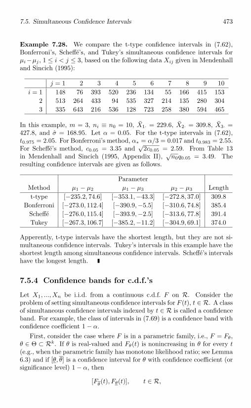
7.5. Simultaneous Confidence Intervals 473
Example 7.28. We compare the t-type confidence intervals in (7.62),Bonferroni’s, Scheffe’s, and Tukey’s simultaneous confidence intervals forµi−µj , 1 ≤ i < j ≤ 3, based on the following data Xij given in Mendenhalland Sincich (1995):
j = 1 2 3 4 5 6 7 8 9 10i = 1 148 76 393 520 236 134 55 166 415 153
2 513 264 433 94 535 327 214 135 280 3043 335 643 216 536 128 723 258 380 594 465
In this example, m = 3, ni ≡ n0 = 10, X1· = 229.6, X2· = 309.8, X3· =427.8, and σ = 168.95. Let α = 0.05. For the t-type intervals in (7.62),t0.975 = 2.05. For Bonferroni’s method, α∗ = α/3 = 0.017 and t0.983 = 2.55.For Scheffe’s method, c0.05 = 3.35 and
√2c0.05 = 2.59. From Table 13
in Mendenhall and Sincich (1995, Appendix II),√n0q0.05 = 3.49. The
resulting confidence intervals are given as follows.
ParameterMethod µ1 − µ2 µ1 − µ3 µ2 − µ3 Lengtht-type [−235.2, 74.6] [−353.1,−43.3] [−272.8, 37.0] 309.8
Bonferroni [−273.0, 112.4] [−390.9,−5.5] [−310.6, 74.8] 385.4Scheffe [−276.0, 115.4] [−393.9,−2.5] [−313.6, 77.8] 391.4Tukey [−267.3, 106.7] [−385.2,−11.2] [−304.9, 69.1] 374.0
Apperently, t-type intervals have the shortest length, but they are not si-multaneous confidence intervals. Tukey’s intervals in this example have theshortest length among simultaneous confidence intervals. Scheffe’s intervalshave the longest length.
7.5.4 Confidence bands for c.d.f.’s
Let X1, ..., Xn be i.i.d. from a continuous c.d.f. F on R. Consider theproblem of setting simultaneous confidence intervals for F (t), t ∈ R. A classof simultaneous confidence intervals indexed by t ∈ R is called a confidenceband. For example, the class of intervals in (7.69) is a confidence band withconfidence coefficient 1 − α.
First, consider the case where F is in a parametric family, i.e., F = Fθ,θ ∈ Θ ⊂ Rk. If θ is real-valued and Fθ(t) is nonincreasing in θ for every t(e.g., when the parametric family has monotone likelihood ratio; see Lemma6.3) and if [θ, θ] is a confidence interval for θ with confidence coefficient (orsignificance level) 1 − α, then
[Fθ(t), Fθ(t)], t ∈ R,
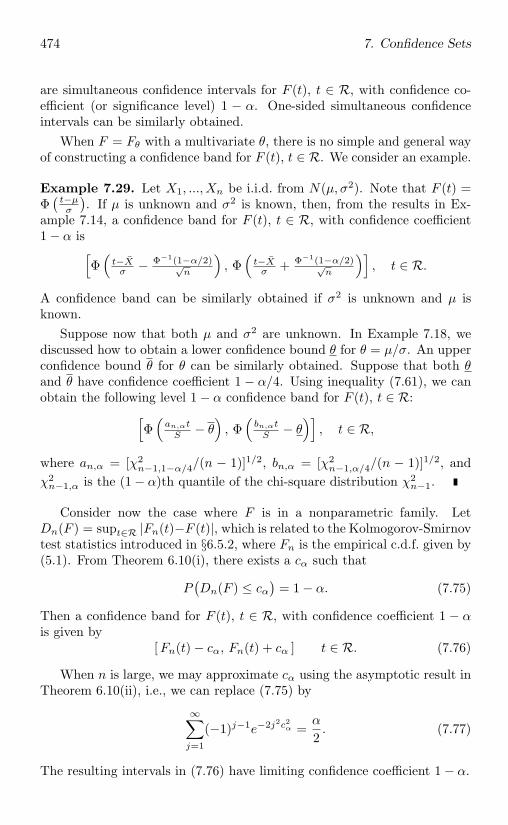
474 7. Confidence Sets
are simultaneous confidence intervals for F (t), t ∈ R, with confidence co-efficient (or significance level) 1 − α. One-sided simultaneous confidenceintervals can be similarly obtained.
When F = Fθ with a multivariate θ, there is no simple and general wayof constructing a confidence band for F (t), t ∈ R. We consider an example.
Example 7.29. Let X1, ..., Xn be i.i.d. from N(µ, σ2). Note that F (t) =Φ
(t−µσ
). If µ is unknown and σ2 is known, then, from the results in Ex-
ample 7.14, a confidence band for F (t), t ∈ R, with confidence coefficient1 − α is[
Φ(
t−Xσ − Φ−1(1−α/2)√
n
), Φ
(t−Xσ + Φ−1(1−α/2)√
n
)], t ∈ R.
A confidence band can be similarly obtained if σ2 is unknown and µ isknown.
Suppose now that both µ and σ2 are unknown. In Example 7.18, wediscussed how to obtain a lower confidence bound θ for θ = µ/σ. An upperconfidence bound θ for θ can be similarly obtained. Suppose that both θand θ have confidence coefficient 1 − α/4. Using inequality (7.61), we canobtain the following level 1 − α confidence band for F (t), t ∈ R:[
Φ(
an,αtS − θ
), Φ
(bn,αtS − θ
)], t ∈ R,
where an,α = [χ2n−1,1−α/4/(n − 1)]1/2, bn,α = [χ2
n−1,α/4/(n − 1)]1/2, andχ2n−1,α is the (1 − α)th quantile of the chi-square distribution χ2
n−1.
Consider now the case where F is in a nonparametric family. LetDn(F ) = supt∈R |Fn(t)−F (t)|, which is related to the Kolmogorov-Smirnovtest statistics introduced in §6.5.2, where Fn is the empirical c.d.f. given by(5.1). From Theorem 6.10(i), there exists a cα such that
P(Dn(F ) ≤ cα
)= 1 − α. (7.75)
Then a confidence band for F (t), t ∈ R, with confidence coefficient 1 − αis given by
[Fn(t) − cα, Fn(t) + cα ] t ∈ R. (7.76)
When n is large, we may approximate cα using the asymptotic result inTheorem 6.10(ii), i.e., we can replace (7.75) by
∞∑j=1
(−1)j−1e−2j2c2α =α
2. (7.77)
The resulting intervals in (7.76) have limiting confidence coefficient 1 − α.
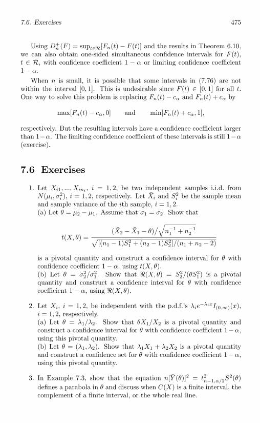
7.6. Exercises 475
Using D+n (F ) = supt∈R[Fn(t) − F (t)] and the results in Theorem 6.10,
we can also obtain one-sided simultaneous confidence intervals for F (t),t ∈ R, with confidence coefficient 1 − α or limiting confidence coefficient1 − α.
When n is small, it is possible that some intervals in (7.76) are notwithin the interval [0, 1]. This is undesirable since F (t) ∈ [0, 1] for all t.One way to solve this problem is replacing Fn(t) − cα and Fn(t) + cα by
max[Fn(t) − cα, 0] and min[Fn(t) + cα, 1],
respectively. But the resulting intervals have a confidence coefficient largerthan 1−α. The limiting confidence coefficient of these intervals is still 1−α(exercise).
7.6 Exercises
1. Let Xi1, ..., Xini, i = 1, 2, be two independent samples i.i.d. from
N(µi, σ2i ), i = 1, 2, respectively. Let Xi and S2
i be the sample meanand sample variance of the ith sample, i = 1, 2.(a) Let θ = µ2 − µ1. Assume that σ1 = σ2. Show that
t(X, θ) =(X2 − X1 − θ)
/√n−1
1 + n−12√
[(n1 − 1)S21 + (n2 − 1)S2
2 ]/(n1 + n2 − 2)
is a pivotal quantity and construct a confidence interval for θ withconfidence coefficient 1 − α, using t(X, θ).(b) Let θ = σ2
2/σ21 . Show that (X, θ) = S2
2/(θS21) is a pivotal
quantity and construct a confidence interval for θ with confidencecoefficient 1 − α, using (X, θ).
2. Let Xi, i = 1, 2, be independent with the p.d.f.’s λie−λixI(0,∞)(x),
i = 1, 2, respectively.(a) Let θ = λ1/λ2. Show that θX1/X2 is a pivotal quantity andconstruct a confidence interval for θ with confidence coefficient 1−α,using this pivotal quantity.(b) Let θ = (λ1, λ2). Show that λ1X1 + λ2X2 is a pivotal quantityand construct a confidence set for θ with confidence coefficient 1−α,using this pivotal quantity.
3. In Example 7.3, show that the equation n[Y (θ)]2 = t2n−1,α/2S2(θ)
defines a parabola in θ and discuss when C(X) is a finite interval, thecomplement of a finite interval, or the whole real line.
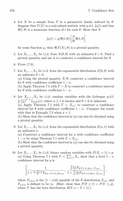
476 7. Confidence Sets
4. Let X be a sample from P in a parametric family indexed by θ.Suppose that T (X) is a real-valued statistic with p.d.f. fθ(t) and that(t, θ) is a monotone function of t for each θ. Show that if
fθ(t) = g((t, θ))∣∣∣∣ ∂∂t(t, θ)
∣∣∣∣for some function g, then (T (X), θ) is a pivotal quantity.
5. Let X1, ..., Xn be i.i.d. from N(θ, θ) with an unknown θ > 0. Find apivotal quantity and use it to construct a confidence interval for θ.
6. Prove (7.3).
7. Let X1, ..., Xn be i.i.d. from the exponential distribution E(0, θ) withan unknown θ > 0.(a) Using the pivotal quantity X/θ, construct a confidence intervalfor θ with confidence coefficient 1 − α.(b) Apply Theorem 7.1 with T = X to construct a confidence intervalfor θ with confidence coefficient 1 − α.
8. Let X1, ..., Xn be i.i.d. random variables with the Lebesgue p.d.f.aθ
(xθ
)a−1I(0,θ)(x), where a ≥ 1 is known and θ > 0 is unknown.
(a) Apply Theorem 7.1 with T = X(n) to construct a confidenceinterval for θ with confidence coefficient 1 − α. Compare the resultwith that in Example 7.2 when a = 1.(b) Show that the confidence interval in (a) can also be obtained usinga pivotal quantity.
9. Let X1, ..., Xn be i.i.d. from the exponential distribution E(a, 1) withan unknown a.(a) Construct a confidence interval for a with confidence coefficient1 − α by using Theorem 7.1 with T = X(1).(b) Show that the confidence interval in (a) can also be obtained usinga pivotal quantity.
10. Let X1, ..., Xn be i.i.d. binary random variables with P (Xi = 1) = p.(a) Using Theorem 7.1 with T =
∑ni=1 Xi, show that a level 1 − α
confidence interval for p is[1
1 + n−T+1T F2(n−T+1),2T,α2
,T+1n−T F2(T+1),2(n−T ),α1
1 + T+1n−T F2(T+1),2(n−T ),α1
],
where Fa,b,α is the (1 − α)th quantile of the F-distribution Fa,b, andFa,0,α is defined to be ∞. (Hint: show that P (T ≥ t) = P (Y ≤ p),where Y has the beta distribution B(T, n− T + 1).)
7.6. Exercises 477
(b) Show that (p, 1] with p given by (7.5) is a level 1 − α confidenceinterval. Compare it with the interval obtained using the result in (a)with α1 = 0.
11. Let X be a sample of size 1 from the negative binomial distributionNB(p, r) with a known r and an unknown p ∈ (0, 1). Using Theorem7.1 with T = X, show that a level 1 − α confidence interval for p is[
11 + T+1
r+1 F2(T+1),2(r+1),α2
,r+1T F2(r+1),2T,α1
1 + r+1T F2(r+1),2T,α1
],
where Fa,b,α is the same as that in the previous exercise.
12. Prove Proposition 7.2.
13. In Example 7.7, show that c(θ) and ci(θ)’s are nondecreasing in θ.
14. Show that the confidence intervals in Example 7.14 and Exercise 1can also be obtained by inverting the acceptance regions of the testsfor one-sample and two-sample problems in §6.2.3.
15. Let Xi, i = 1, 2, be independently distributed as the binomial distri-butions Bi(pi, ni), i = 1, 2, respectively, where ni’s are known andpi’s are unknown. Show how to invert the acceptance regions of theUMPU tests in Example 6.11 to obtain a level 1−α confidence intervalfor the odds ratio p2(1−p1)
p1(1−p2).
16. Let X1, ..., Xn be i.i.d. from N(µ, σ2).(a) Suppose that σ2 = γµ2 with unknown γ > 0 and µ ∈ R. Obtaina confidence set for γ with confidence coefficient 1 − α by invertingthe acceptance regions of LR tests for H0 : γ = γ0 versus H1 : γ = γ0.(b) Repeat (a) when σ2 = γµ with unknown γ > 0 and µ > 0.
17. Consider the problem in Example 6.17. Discuss how to construct aconfidence interval for θ with confidence coefficient 1 − α by(a) inverting the acceptance regions of the tests derived in Example6.17;(b) applying Theorem 7.1.
18. Let X1, ..., Xn be i.i.d. from the uniform distribution U(θ− 12 , θ+ 1
2 ).Construct a confidence interval for θ with confidence coefficient 1−α.
19. Let X1, ..., Xn be i.i.d. binary random variables with P (Xi = 1) = p.Using the p.d.f. of the beta distribution B(a, b) as the prior p.d.f.,construct a level 1 − α HPD credible set for p.
478 7. Confidence Sets
20. Let X1, ..., Xn be i.i.d. from N(µ, σ2) with an unknown θ = (µ, σ2).Consider the prior p.d.f. π(θ) = π1(µ|σ2)π2(σ2), where π1(µ|σ2) isthe p.d.f. of N(µ0, σ
20σ
2),
π2(σ2) =1
Γ(a)ba
(1σ2
)a+1
e−1/(bσ2)I(0,∞)(σ2),
and µ0, a, and b are known.(a) Find the posterior of µ and construct a level 1 − α HPD credibleset for µ.(b) Show that the credible set in (a) approaches the confidence intervalobtained in Example 7.14 as σ2
0 , a, and b approach some limits.
21. Let X1, ..., Xn be i.i.d. with a Lebesgue p.d.f. 1σf
(x−µσ
), where f is
a known p.d.f. and µ and σ > 0 are unknown. Let X0 be a futureobservation that is independent of Xi’s and has the same distributionas Xi. Find a pivotal quantity (X,X0) and construct a level 1 − αprediction set for X0.
22. Let X1, ..., Xn be i.i.d. from a continuous c.d.f. F on R and X0be a future observation that is independent of Xi’s and has thec.d.f. F . Suppose that F is strictly increasing in a neighborhoodof F−1(α/2) and a neighborhood of F−1(1 − α/2). Let Fn be theempirical c.d.f. defined by (5.1). Show that the prediction intervalC(X) = [F−1
n (α/2), F−1n (1 − α/2)] for X0 satisfies P (X0 ∈ C(X)) →
1 − α, where P is the joint distribution of (X0, X1, ..., Xn).
23. Let X1, ..., Xn be i.i.d. with a Lebesgue p.d.f. f(x − µ), where f isknown and µ is unknown.(a) If f is the p.d.f. of the standard normal distribution, show that theconfidence interval [X− c1, X + c1] is better than [X1− c2, X1 + c2] interms of their lengths, where ci’s are chosen so that these confidenceintervals have confidence coefficient 1 − α.(b) If f is the p.d.f. of the Cauchy distribution C(0, 1), show that thetwo confidence intervals in (a) have the same length.
24. Prove Theorem 7.3(ii).
25. Show that the expected length of the interval in (7.13) is shorter thanthe expected length of the interval in (7.12).
26. Consider Example 7.14.(a) Suppose that θ = σ2 and µ is known. Let a∗ and b∗ be constantssatisfying a2
∗g(a∗) = b2∗g(b∗) > 0 and∫ b∗a∗
g(x)dx = 1 − α, where g isthe p.d.f. of the chi-square distribution χ2
n. Show that the interval[b−1
∗ T, a−1∗ T ] has the shortest length within the class of intervals of
7.6. Exercises 479
the form [b−1T, a−1T ],∫ b
ag(x)dx = 1−α, where T =
∑ni=1(Xi−µ)2.
(b) Show that the expected length of the interval in (a) is shorterthan the expected length of the interval in (7.14).(c) Find the shortest-length interval for θ = σ within the class ofconfidence intervals of the form [b−1/2√n− 1S, a−1/2√n− 1S], where0 < a < b < ∞ and
∫ b
af(x)dx = 1 − α.
27. Assume the conditions in Theorem 7.3(i). Assume further that fis symmetric. Show that a∗ and b∗ in Theorem 7.3(i) must satisfya∗ = −b∗.
28. Let f be a Lebesgue p.d.f. that is nonzero in [x−, x+] and is 0 outside[x−, x+], −∞ ≤ x− < x+ ≤ ∞.(a) Suppose that f is strictly dereasing. Show that, among all in-tervals [a, b] satisfying
∫ b
af(x)dx = 1 − α, the shortest interval is
obtained by choosing a = x− and b so that∫ b
x−f(x)dx = 1 − α.
(b) Obtain a result similar to that in (a) when f is strictly increasing.Use the result to show that the interval [X(n), α
−1/nX(n)] in Example7.13 has the shortest length among all intervals [b−1X(n), a
−1X(n)].
29. Let X1, ..., Xn be i.i.d. from the exponential distribution E(a, 1) withan unknown a. Find a confidence interval for a having the shortestlength within the class of confidence intervals [X(1) + c,X(1) +d] withconfidence coefficient 1 − α.
30. Consider the HPD credible set C(x) in (7.7) for a real-valued θ. Sup-pose that px(θ) is a unimodal Lebesgue p.d.f. and is not monotone.Show that C(x) is an interval having the shortest length within theclass of intervals [a, b] satisfying
∫ b
apx(θ)dθ = 1 − α.
31. Let X be a single observation from the gamma distribution Γ(α, γ)with a known α and an unknown γ. Find the shortest-length confi-dence interval within the class of confidence intervals [b−1X, a−1X]with a given confidence coefficient.
32. Let X1, ..., Xn be i.i.d. with the Lebesgue p.d.f. θxθ−1I(0,1)(x), whereθ > 0 is unknown.(a) Construct a confidence interval for θ with confidence coefficient1 − α, using a sufficient statistic.(b) Discuss whether the confidence interval obtained in (a) has theshortest length within a class of confidence intervals.(c) Discuss whether the confidence interval obtained in (a) is UMAU.
33. Let X be a single observation from the logistic distribution LG(µ, 1)with an unknown µ ∈ R. Find a Θ′-UMA upper confidence boundfor µ with confidence coefficient 1 − α, where Θ′ = (µ,∞).
480 7. Confidence Sets
34. Let X1, ..., Xn be i.i.d. from the exponential distribution E(0, θ) withan unknown θ > 0. Find a Θ′-UMA lower confidence bound for θwith confidence coefficient 1 − α, where Θ′ = (0, θ).
35. Let X be a single observation from N(θ − 1, 1) if θ < 0, N(0, 1) ifθ = 0, and N(θ + 1, 1) if θ > 0.(a) Show that the distribution of X is in a family with monotonelikelihood ratio.(b) Construct a Θ′-UMA lower confidence bound for θ with confidencecoeffcient 1 − α, where Θ′ = (−∞, θ).
36. Show that the confidence set in Example 7.9 is unbiased.
37. In Example 7.13, show that the confidence interval [X(n), α−1/nX(n)]
is UMA and has the shortest expected length among all confidenceintervals for θ with confidence coefficient 1 − α.
38. Let X1, ..., Xn be i.i.d. from the exponential distribution E(a, θ) withunknown a and θ. Find a UMAU confidence interval for a with con-fidence coefficient 1 − α.
39. Let Y and U be independent having the binomial distribution Bi(p, n)and the uniform distribution U(0, 1), respectively.(a) Show that W = Y + U has the Lebesgue p.d.f. fp(w) given by(7.17).(b) Show that the family fp : p ∈ (0, 1) has monotone likelihoodratio in W .
40. Let X1, ..., Xn be i.i.d. from the Poisson distribution P (θ) with anunknown θ > 0. Find a randomized UMA upper confidence boundfor θ with confidence coefficient 1 − α.
41. Let X1, ..., Xn be i.i.d. from N(µ, σ2) with unknown µ and σ2.(a) Show that θ = X + tn−1,αS/
√n is a UMAU upper confidence
bound for µ with confidence coefficient 1 − α, where tn−1,α is the(1 − α)th quantile of the t-distribution tn−1.(b) Show that the confidence bound in (a) can be derived by invertingacceptance regions of LR tests.
42. Prove Theorem 7.7 and Proposition 7.3.
43. Let X1, ..., Xn be i.i.d. with p.d.f. f(x − θ), where f is a knownLebesgue p.d.f. Show that the confidence interval [X − c1, X + c2]has constant coverage probability, where c1 and c2 are constants.
44. Prove the claim in Example 7.18.
7.6. Exercises 481
45. In Example 7.19, show that(a) the testing problem is invariant under Gµ0 , but not G;(b) the nonrandomized test with acceptance region A(µ0) is UMPamong unbiased and invariant tests of size α, under Gµ0 ;(c) G is the smallest group containing ∪µ0∈RGµ0 .
46. In Example 7.17, show that intervals (7.13) and (7.14) are UMAamong unbiased and invariant confidence intervals with confidencecoefficient 1 − α, under G1 and G, respectively.
47. Let Xi, i = 1, 2, be independent with the exponential distributionsE(0, θi), i = 1, 2, respectively.(a) Show that [αY/(2−α), (2−α)Y/α] is a UMAU confidence intervalfor θ2/θ1 with confidence coefficient 1 − α, where Y = X2/X1.(b) Show that the confidence interval in (a) is also UMAI.
48. Let X1, ..., Xn be i.i.d. from a bivariate normal distribution with un-known mean and covariance matrix and let R(X) be the sample corre-lation coefficient. Define ρ = C−1(R(X)), where C(ρ) is determinedby
P(R(X) ≤ C(ρ)
)= 1 − α
and ρ is the unknown correlation coefficient. Show that ρ is a Θ′-UMAI lower confidence bound for ρ with confidence coefficient 1−α,where Θ′ = (−1, ρ).
49. Let Xi1, ..., Xini, i = 1, 2, be two independent samples i.i.d. from
N(µi, σ2), i = 1, 2, respectively, where µi’s are unknown. Find a
UMAI confidence interval for µ2−µ1 with confidence coefficient 1−αwhen (a) σ2 is known; (b) σ2 is unknown.
50. In Example 7.23, show that C3(X) = [p−, p+] with the given p±.Compare the lengths of the confidence intervals C2(X) and C3(X).
51. Show that the confidence intervals in Example 7.14 can be derived byinverting acceptance regions of LR tests.
52. Let X1, ..., Xn be i.i.d. from the exponential distribution E(0, θ) withan unknown θ > 0.(a) Show that (X, θ) =
√n(X−θ)/θ is asymptotically pivotal. Con-
struct a 1 − α asymptotically correct confidence interval for θ, using(X, θ).(b) Show that 1(X, θ) =
√n(X − θ)/X is asymptotically pivotal.
Construct a 1 − α asymptotically correct confidence interval for θ,using 1(X, θ).(c) Obtain 1 − α asymptotically correct confidence intervals for θ by
482 7. Confidence Sets
inverting acceptance regions of LR tests, Wald’s tests, and Rao’s scoretests.
53. Let X1, ..., Xn be i.i.d. from the Poisson distribution P (θ) with anunknown θ > 0.(a) Show that (X, θ) = (X − θ)/
√θ/n is asymptotically pivotal.
Construct a 1 − α asymptotically correct confidence interval for θ,using (X, θ).(b) Show that 1(X, θ) = (X − θ)/
√X/n is asymptotically pivotal.
Construct a 1 − α asymptotically correct confidence interval for θ,using 1(X, θ).(c) Obtain 1 − α asymptotically correct confidence intervals for θ byinverting acceptance regions of LR tests, Wald’s tests, and Rao’s scoretests.
54. Let Xi1, ..., Xini , i = 1, 2, be two independent samples i.i.d. fromN(µi, σ
2i ), i = 1, 2, respectively, where all parameters are unknown.
Show that (X,µ1−µ2) = (X1·−X2·−µ1 +µ2)/√n−1
1 S21 + n−1
2 S22 is
asymptotically pivotal, assuming that n1/n2 → c ∈ (0,∞). Constructa 1 − α asymptotically correct confidence interval for µ1 − µ2 using(X,µ1 − µ2).
55. Consider the problem in Example 5.15. Construct an asymptoticallypivotal quantity and a 1−α asymptotically correct confidence set forθ. Compare this confidence set with those in Example 7.24.
56. Consider the problem in Example 3.21. Construct an asymptoticallypivotal quantity and a 1−α asymptotically correct confidence set forµy/µx.
57. Consider the problem in Example 3.23. Construct an asymptoticallypivotal quantity and a 1−α asymptotically correct confidence set forR(t) with a fixed t.
58. Let Un be a U-statistic based on i.i.d. X1, ..., Xn and the kernelh(x1, ..., xm), and let θ = E(Un). Construct an asymptotically pivotalquantity based on Un and a 1 − α asymptotically correct confidenceset for θ.
59. Let X1, ..., Xn be i.i.d. from a c.d.f. F on R that is continuous andsymmetric about θ. Let θ = W/n− 1
2 and T(F ) = θ+ 12 , where W and
T are given by (6.78) and (5.46), respectively. Construct a confidenceinterval for θ that has limiting confidence coefficient 1 − α.
60. Consider the linear model X = βZτ + ε, where ε has independentcomponents with mean 0 and Z is of full rank. Assume the conditions
7.6. Exercises 483
in Theorem 3.12.(a) Suppose that Var(ε) = σ2D, where D is a known diagonal matrixand σ2 is unknown. Find an asymptotically pivotal quantity andconstruct a 1 − α asymptotically correct confidence set for β.(b) Suppose that Var(ε) is an unknown diagonal matrix. Find anasymptotically pivotal quantity and construct a 1−α asymptoticallycorrect confidence set for β.
61. Consider a GEE estimator θ of θ described in §5.4.1. Discuss how toconstruct an asymptotically pivotal quantity and a 1 − α asymptoti-cally correct confidence set for θ. (Hint: see §5.5.2.)
62. Suppose that X1, ..., Xn are i.i.d. from the negative binomial distri-bution NB(p, r) with a known r and an unknown p. Obtain 1 − αasymptotically correct confidence intervals for p by inverting accep-tance regions of LR tests, Wald’s tests, and Rao’s score tests.
63. Let X1, ..., Xn be i.i.d. from the exponential distribution E(a, θ) withunknown a and θ. Find a 1−α asymptotically correct confidence setby inverting acceptance regions of LR tests.
64. Let Xi1, ..., Xini , i = 1, 2, be two independent samples i.i.d. fromN(µi, σ
2), i = 1, 2, respectively, where all parameters are unknown.(a) Find 1 − α asymptotically correct confidence sets for (µ1, µ2) byinverting acceptance regions of LR tests, Wald’s tests, and Rao’s scoretests.(b) Repeat (a) for the parameter (µ1, µ2, σ
2).
65. Let Xi1, ..., Xini , i = 1, 2, be two independent samples i.i.d. fromN(µi, σ
2i ), i = 1, 2, respectively, where all parameters are unknown.
(a) Find 1 − α asymptotically correct confidence sets for (µ1, µ2) byinverting acceptance regions of LR tests, Wald’s tests, and Rao’s scoretests.(b) Repeat (a) for the parameter (µ1, µ2, σ
21 , σ
22).
66. Let Xi1, ..., Xini , i = 1, 2, be two independent samples i.i.d. from theexponential distributions E(0, θi), i = 1, 2, respectively, where θi’sare unknown. Find 1 − α asymptotically correct confidence sets for(θ1, θ2) by inverting acceptance regions of LR tests, Wald’s tests, andRao’s score tests.
67. Consider the problem in Example 7.9. Find 1 − α asymptoticallycorrect confidence sets for θ by inverting acceptance regions of LRtests, Wald’s tests, and Rao’s score tests. Which one is the same asthat derived in Example 7.9?
484 7. Confidence Sets
68. Let X1, ..., Xn be i.i.d. from a continuous c.d.f. F on R and let θ =F−1(p), p ∈ (0, 1).(a) Show that P (X(k1) ≤ θ ≤ X(k2)) = P (U(k1) ≤ p ≤ U(k2)), whereX(k) is the kth order statistic and U(k) is the kth order statistic basedon a sample U1, ..., Un i.i.d. from the uniform distribution U(0, 1).(b) Show that
P (U(k1) ≤ p ≤ U(k2)) = Bp(k1, n− k1 + 1) −Bp(k2, n− k2 + 1),
where
Bp(i, j) =Γ(i + j)Γ(i)Γ(j)
∫ p
0ti−1(1 − t)j−1dt.
(c) Discuss how to obtain a confidence interval for θ with confidencecoefficient 1 − α.
69. Prove Corollary 7.1.
70. Assume the conditions in Corollary 7.1.(a) Show that
√n(X(kn) − θ)F ′(θ) →d N(c, p(1 − p)).
(b) Prove result (7.24) using the result in part (a).(c) Construct a consistent estimator of the asymptotic variance of thesample median (see Example 6.27), using Woodruff’s interval.
71. Show that θHB in (7.32) is equal to 2θn −K−1B (1 − α), where KB is
defined in (7.25).
72. (Parametric bootstrapping in location-scale families). Let X1, ..., Xn
be i.i.d. random variables with p.d.f. 1σf
(x−µσ
), where f is a known
Lebesgue p.d.f. and µ and σ > 0 are unknown. Let X∗1 , ..., X
∗n be
i.i.d. bootstrap data from the p.d.f. 1sf
(x−xs
), where x and s2 are the
observed sample mean and sample variance, respectively.(a) Suppose that we construct the bootstrap-t lower confidence bound(7.33) for µ using the parametric bootstrap data. Show that θBT hasconfidence coefficient 1 − α.(b) Suppose that we construct the hybrid bootstrap lower confidencebound (7.32) for µ using the parametric bootstrap data. Show thatθHB does not necessarily have confidence coefficient 1 − α.(c) Suppose that f has mean 0 and variance 1. Show that θHB in (b)is 1 − α asymptotically correct.
73. (The bootstrap BCa percentile method). Suppose that we changeassumption (7.28) to
P
(φn − φn(θ)1 + aφn(θ)
+ z0 ≤ x
)= Ψ(x),
7.6. Exercises 485
where a is an extra parameter called the acceleration constant.(a) If φn, z0, a, and Φ are known, show that the following lowerconfidence bound for θ has confidence coefficient 1 − α:
θE = φ−1n
(φn + (zα + z0)(1 + aφn)/[1 − a(zα + z0)]
).
(b) Show that K−1B (x) = φ−1
n
(φn + [Φ−1(x) − z0](1 + aφn)
), where
KB is defined in (7.25).(c) Let θBC(a) = K−1
B
(Φ(z0 + (zα + z0)/[1 − a(zα + z0)])
). Show
that θBC(a) = θE in part (a). (The bootstrap BCa percentile lowerconfidence bound for θ is θBC(a), where a is an estimator of a.)
74. (Automatic bootstrap percentile). Let P = Pθ : θ ∈ R be a para-metric family. Define Kθ(x) = Pθ(θn ≤ x), where θn is an estimatorof θ. Let θ0 be a given value of θ and θ1 = K−1
θ0(1−α). The automatic
bootstrap percentile lower confidence bound for θ is defined to be
θABP = K−1θn
(Kθ1(θ0)).
Assume the assumption in the previous exercise. Show that θABP
has confidence coefficient 1 − α.
75. (Bootstrapping residuals). Consider linear model (3.25): X = βZτ +ε, where Z is of full rank and ε is a vector of i.i.d. random variableshaving mean 0 and variance σ2. Let ri = Xi−βZτ
i be the ith residual,where β is the LSE of β. Assume that the average of ri’s is always 0.Let ε∗1, ..., ε
∗n be i.i.d. bootstrap data from the empirical c.d.f. putting
mass n−1 on each ri. Define X∗i = βZτ
i + ε∗i , i = 1, ..., n.(a) Find an expression for β∗, the bootstrap analogue of β. CalculateE(β∗|X) and Var(β∗|X).(b) Using (β − β)lτ and the idea in §7.4.1, construct a hybrid boot-strap lower confidence bound for βlτ , where l ∈ Rp.(c) Discuss when the lower confidence bound in (b) is 1 − α asymp-totically correct.(d) Describe how to construct a bootstrap-t lower confidence boundfor βlτ .(e) Describe how to construct a hybrid bootstrap confidence set forβ, using the idea in §7.4.1.
76. (Bootstrapping pairs). Consider linear model (3.25): X = βZτ + ε,where Z is of full rank and ε is a vector of independent random vari-ables having mean 0 and finite variances. Let (X∗
1 , Z∗1 ), ..., (X∗
n, Z∗n)
be i.i.d. bootstrap data from the empirical c.d.f. putting mass n−1 oneach (Xi, Zi). Define β∗ =
∑ni=1 X
∗i Z
∗i (ZτZ)−1. Repeat (a)-(e) of
the previous exercise.
486 7. Confidence Sets
77. (External bootstrapping or wild bootstrapping). Assume the modelin the previous exercise. Let ε∗1, ..., ε
∗n be i.i.d. random variables with
mean 0 and variance 1. Define the bootstrap data as X∗i = βZτ
i +|ti|ε∗i , i = 1, ..., n, where β is the LSE of β, ti = (Xi − βZτ
i )/√
1 − hi,and hi = Zi(ZτZ)−1Zτ
i . Repeat (a)-(e) of Exercise 75.
78. Prove (7.48) and (7.49).
79. Using the Edgeworth expansion given in Example 7.25, construct athird-order accurate lower confidence bound for µ. (Hint: use (7.50)and (7.51).)
80. Describe how to approximate C(3)PREB(X) in (7.53), using the Monte
Carlo method.
81. Prove (7.55) and (7.56).
82. Show that Bonferroni’s simultaneous confidence intervals are of level1 − α.
83. Let Ct,α(X) be a confidence interval for θt with confidence coefficient1−α, t = 1, ..., k. Suppose that C1,α(X), ..., Ck,α(X) are independentfor any α. Show how to construct simultaneous confidence intervalsfor θt, t = 1, ..., k, with confidence coefficient 1 − α.
84. Show that Cij,α(X) in (7.62) is UMAU for µi − µj .
85. Consider the two-way balanced ANOVA model in Example 6.19. Us-ing Bonferroni’s method, obtain level 1 − α simultaneous confidenceintervals for(a) αi, i = 1, ..., a− 1;(b) µij , i = 1, ..., a, j = 1, ..., b.
86. Prove (7.64). (Hint: use the Cauchy-Schwarz inequality.)
87. Let x ∈ Rk, y ∈ Rk, and A be a k × k positive definite matrix.(a) Suppose that yA−1xτ = 0. Show that
xA−1xτ = maxc∈Rk,c =0,cyτ=0
(cxτ )2
cAcτ.
(b) Assume model (7.63) with a full rank Z. Using the result in (a),construct simultaneous confidence intervals (with confidence coeffi-cient 1 − α) for βcτ , c ∈ Rp, c = 0, cyτ = 0, where y ∈ Rp satisfyingyZτZ = 0.
88. Assume the conditions in Theorem 3.12. Show that Scheffe’s intervalsin Theorem 7.10 are 1 − α asymptotically correct.
7.6. Exercises 487
89. Prove (7.67).
90. Find explicitly the m(m − 1)/2 vectors in the set T0 in (7.68) sothat βLτ tτ : t ∈ T0 is exactly the same as µi − µj , 1 ≤ i < j ≤ m.Show that the intervals in (7.68) are Scheffe’s simultaneous confidenceintervals.
91. In Example 7.27, show that(a) Scheffe’s intervals in Theorem 7.10 with t = (1, x) and L = I2 areof the form (7.69);(b) the maximum on the right-hand side of (7.70) is achieved at (y, x)given by (7.71);(c) y in (7.71) is equal to 1.
92. Consider the two-way balanced ANOVA model in Example 6.19. Us-ing Scheffe’s method, obtain level 1 − α simultaneous confidence in-tervals for αi’s, βj ’s, and γij ’s.
93. Let Xij = N(µ+αi +βj , σ2), i = 1, ..., a, j = 1, ..., b, be independent,
where∑a
i=1 αi = 0 and∑b
j=1 βj = 0. Construct level 1 − α simulta-neous confidence intervals for all linear combinations of αi’s and βj ’s,using(a) Bonferroni’s method;(b) Scheffe’s method.
94. Assume model (7.63) with β = (β0, β1, β2) and Zi = (1, ti, t2i ), whereti ∈ R,
∑ni=1 ti = 0,
∑ni=1 t
2i = 1, and
∑ni=1 t
3i = 0.
(a) Construct a confidence ellipsoid for (β1, β2) with confidence coef-ficient 1 − α;(b) Construct simultaneous confidence intervals for all linear combi-nations of β1 and β2, with confidence coefficient 1 − α.
95. Show that the distribution of Rst in (7.72) does not depend on anyunknown parameter.
96. For α = 0.05, obtain numerically the t-type confidence intervals in(7.62), Bonferroni’s, Scheffe’s, and Tukey’s simultaneous confidenceintervals for µi − µj , 1 ≤ i < j ≤ 4, based on the following data Xij
from a one-way ANOVA model (q0.05 = 4.45):
j = 1 2 3 4 5 6i = 1 0.08 0.10 0.09 0.07 0.09 0.06
2 0.15 0.09 0.11 0.10 0.08 0.133 0.13 0.10 0.15 0.09 0.09 0.174 0.05 0.11 0.07 0.09 0.11 0.08
488 7. Confidence Sets
97. (Dunnett’s simultaneous confidence intervals). Let X0j (j = 1, ..., n0)and Xij (i = 1, ...,m, j = 1, ..., n0) represent independent measure-ments on a standard and m competing new treatments. Supposethat Xij = N(µi, σ
2) with unknown µi and σ2 > 0, i = 0, 1, ...,m.Let Xi· be the sample mean based on Xij , j = 1, ..., n0, and σ2 =[(m + 1)(n0 − 1)]−1 ∑m
i=0∑n0
j=1(Xij − Xi·)2.(a) Show that the distribution of
Rst = maxi=1,...,m
|(Xi· − µi) − (X0· − µ0)|/σ
does not depend on any unknown parameter.(b) Show that[
m∑i=0
ciXi· − qασ
m∑i=1
|ci|,m∑i=0
ciXi· + qασ
m∑i=1
|ci|]
for all c0, c1, ..., cm satisfying∑m
i=0 ci = 0 are simultaneous confidenceintervals for
∑mi=0 ciµi with confidence coefficient 1 − α, where qα is
the (1 − α)th quantile of Rst.
98. Let X1, ..., Xn be i.i.d. from the uniform distribution U(0, θ), whereθ > 0 is unknown. Construct a confidence band for the c.d.f. of X1with confidence coefficient 1 − α.
99. Let X1, ..., Xn be i.i.d. with the p.d.f. 1σf
(t−µσ
), where f is a known
Lebesgue p.d.f. (a location-scale family). Let F be the c.d.f. of X1.(a) Suppose that µ is unknown and σ > 0 is known. Constructsimultaneous confidence intervals for F (t), t ∈ R, with confidencecoefficient 1 − α.(b) Suppose that µ is known and σ > 0 is unknown. Constructsimultaneous confidence intervals for F (t), t ∈ R, with confidencecoefficient 1 − α.(c) Suppose that both µ and σ > 0 are unknown. Construct level1 − α simultaneous confidence intervals for F (t), t ∈ R.
100. Let X1, ..., Xn be i.i.d. from F on R and Fn be the empirical c.d.f.Show that the intervals[
max[Fn(t) − cα, 0], min[Fn(t) + cα, 1]], t ∈ R,
form a confidence band for F (t), t ∈ R, with limiting confidencecoefficient 1 − α, where cα is given by (7.77).
Appendix A
Abbreviations
a.e.: almost everywhere.
amse: asymptotic mean squarederror.
ANOVA: analysis of variance.
a.s.: almost surely.
BC: bias-corrected.
BCa: accelerated bias-corrected.
BLUE: best linear unbiased estima-tor.
c.d.f.: cumulative distribution func-tion.
ch.f.: characteristic function.
CLT: central limit theorem.
GEE: generalized estimation equa-tion.
GLM: generalized linear model.
HPD: highest posterior density.
i.i.d.: independent and identicallydistributed.
LR: likelihood ratio.
LSE: least squares estimator.
MCMC: Markov chain MonteCarlo.
MELE: maximum empirical likeli-hood estimator.
m.g.f.: moment generating func-tion.
MLE: maximum likelihood estima-tor.
MQLE: maximum quasi-likelihoodestimator.
MRIE: minimum risk invariant es-timator.
mse: mean squared error.
p.d.f.: probability density function.
RLE: root of likelihood equation.
SLLN: strong law of large numbers.
UMA: uniformly most accurate.
UMAI: uniformly most accurateinvariant.
UMAU: uniformly most accurateunbiased.
UMP: uniformly most powerful.
489

490 Appendix A. Abbreviations
UMPI: uniformly most powerfulinvariant.
UMPU: uniformly most powerfulunbiased.
UMVUE: uniformly minimum vari-ance unbiased estimator.
WLLN: weak law of large numbers.
w.r.t.: with respect to.
Appendix B
Notation
R: the real line.
Rk: the k-dimensional Euclideanspace.
B: the Borel σ-field on R.
Bk: the Borel σ-field on Rk.
(a, b) and [a, b]: the open and closedintervals from a to b.
a, b: the set consisting of the ele-ments a and b.
Aτ : the transpose of a matrix or avector A.
Det(A): the determinant of a ma-trix A.
tr(A): the trace of a matrix A.
A−1: the inverse of a matrix A.
A1/2: the square root of a nonneg-ative definite matrix A definedby A1/2A1/2 = A.
A−1/2: the inverse of A1/2.
Ik: the k × k identity matrix.
‖x‖: the Euclidean norm of a vec-tor x ∈ Rk, ‖x‖2 = xxτ .
IA: the indicator function of the setA.
Ac: the complement of the set A.
P (A): the probability of the set A.
an: a sequence of vectors or ran-dom vectors a1, a2, ....
an → a: an converges to a as nincreases to ∞.
→a.s.: convergence almost surely.
→p: convergence in probability.
→d: convergence in distribution.
g′, g′′, and g(k): the first-, second-,and kth-order derivatives of afunction g on R.
g(x+) or g(x−): the right or theleft limit of the function g atx.
∂g/∂x or ∇g: the partial derivativerow vector of the function g onRk.
∂2g/∂x∂xτ or ∇2g: the second-order partial derivative matrixof the function g on Rk.
491
492 Appendix B. Notation
F−1(p): the pth quantile of a c.d.f.F , F−1(t)=infx : F (x) ≥ t.
E(X) or EX: the expectation ofa random variable (vector ormatrix) X.
Var(X): the variance (covariancematrix) of a random variable(vector) X.
Cov(X,Y ): the covariance betweenrandom variables X and Y .
P: a family containing the popula-tion P that generates data
bT (P ): the bias of an estimator Tunder population P .
bT (P ): an asymptotic bias of an es-timator T under population P .
mseT (P ): the mse of an estimatorT under population P .
RT (P ): the risk of an estimator Tunder population P .
amseT (P ): an asymptotic mse ofan estimator T under popula-tion P .
eT ′n,Tn(P ): the asymptotic relative
efficiency of T ′n w.r.t. Tn.
αT (P ): probability of type I errorfor a test T .
βT (P ): power function for a test T .
X(i): the ith order statistic of X1,..., Xn.
X: the sample mean of X1, ..., Xn,
X =∑n
i=1Xi
n .
S2 : the sample variance (covari-ance matrix) of X1, ..., Xn,
S2 =∑n
i=1(Xi−X)τ (Xi−X)
n−1 .
Fn: the empirical c.d.f. based onX1, ..., Xn.
N(µ, σ2): the one-dimensional nor-mal distribution or randomvariable with mean µ and vari-ance σ2.
Nk(µ,Σ): the k-dimensional nor-mal distribution or randomvector with mean vector µ andcovariance matrix Σ.
Φ(x): the standard normal c.d.f.
zα: the αth quantile of the stan-dard normal distribution.
χ2r: a random variable having the
chi-square distribution χ2r.
χ2r,α: the (1 − α)th quantile of the
chi-square distribution χ2r.
tr,α: the (1 − α)th quantile of thet-distribution tr.
Fa,b,α: the (1−α)th quantile of theF-distribution Fa,b.

References
We provide some references for further readings of the topics covered inthis book.
For a general probability theory, Billingsley (1986) and Chung (1974)are suggested, although there are many standard textbooks. An asymptotictheory for statistics can be found in Serfling (1980), Shorack and Wellner(1986), Sen and Singer (1993), and Barndorff-Nielsen and Cox (1994).
More discussions of fundamentals of statistical decision theory and in-ference can be found in many textbooks on mathematical statistics, such asCramer (1946), Wald (1950), Savage (1954), Ferguson (1967), Rao (1973),Rohatgi (1976), Bickel and Doksum (1977), Lehmann (1986), Casella andBerger (1990), and Barndorff-Nielsen and Cox (1994). Discussions andproofs for results related to sufficiency and completeness can be found inRao (1945), Blackwell (1947), Hodges and Lehmann (1950), Lehmann andScheffe (1950), and Basu (1955). More results for exponential families aregiven in Barndorff-Nielsen (1979).
The theory of UMVUE in §3.1.1 and §3.1.2 is mainly based on Chapter2 of Lehmann (1983). More results on information inequalities can befound in Cramer (1946), Rao (1973), Lehmann (1983), and Pitman (1979).The theory of U-statistics and the method of projection can be found inHoeffding (1948), Randles and Wolfe (1979), and Serfling (1980). Therelated theory for V-statistics is given in von Mises (1947), Serfling (1980),and Sen (1981). Three excellent textbooks for the theory of LSE are Scheffe(1959), Searle (1971), and Rao (1973). Additional materials for samplesurveys can be found in Basu (1958), Godambe (1958), Cochran (1977),Sarndal, Swensson, and Wretman (1992), and Ghosh and Meeden (1997).
Excellent textbooks for the Bayesian theory include Lindley (1965), Boxand Tiao (1973), Berger (1985), and Schervish (1995). For Bayesian com-putation and Markov chain Monte Carlo, more discussions can be found inreferences cited in §4.1.4. More general results on invariance in estimationand testing problems are provided by Ferguson (1967) and Lehmann (1983,1986). The theory of shrinkage estimation was established by Stein (1956)
493
494 References
and James and Stein (1961); Lehmann (1983) and Berger (1985) provideexcellent discussions on this topic. The method of likelihood has more than200 years of history (Edwards, 1974). An excellent textbook on the MLEin generalized linear models is McCullagh and Nelder (1989). Asymptoticproperties for MLE can be found in Cramer (1946), Serfling (1980), and Senand Singer (1993). Asymptotic results for the MLE in generalized linearmodels are provided by Fahrmeir and Kaufmann (1985).
An excellent book containing results for empirical c.d.f.’s and their prop-erties is Shorack and Wellner (1986). References for empirical likelihoodsare provided in §5.1.2 and §6.5.3. More results in density estimation canbe found, for example, in Rosenblatt (1971) and Silverman (1986). Morediscussions on statistical functionals can be found in von Mises (1947), Ser-fling (1980), Fernholz (1983), Sen and Singer (1993), and Shao and Tu(1995). Two textbooks for robust statistics are Huber (1981) and Hampelet al. (1986). A general discussion of L-estimators and sample quantiles canbe found in Serfling (1980) and Sen (1981). L-estimators in linear modelsare covered by Bickel (1973), Puri and Sen (1985), Welsh (1987), and Heand Shao (1996). Some references on generalized estimation equations andquasi-likelihoods are Godambe and Heyde (1987), Godambe and Thompson(1989), McCullagh and Nelder (1989), and Diggle, Liang, and Zeger (1994).Two textbooks containing materials on variance estimation are Efron andTibshirani (1993) and Shao and Tu (1995).
The theory of UMP, UMPU, and UMPI tests in Chapter 6 is mainlybased on Lehmann (1986) and Chapter 5 of Ferguson (1967). Berger (1985)contains discussion on Bayesian tests. Results on large sample tests andchi-square tests can be found in Serfling (1980) and Sen and Singer (1993).Two textbooks on nonparametric tests are Lehmann (1975) and Randlesand Wolfe (1979).
Further materials on confidence sets can be found in Ferguson (1967),Bickel and Doksum (1977), Lehmann (1986), and Casella and Berger (1990).More results on asymptotic confidence sets based on likelihoods can befound in Serfling (1980). The theory of bootstrap confidence sets is cov-ered by Hall (1992), Efron and Tibshirani (1993), and Shao and Tu (1995).Further discussions on simultaneous confidence intervals can be found inScheffe (1959), Lehmann (1986), and Tukey (1977).
The following references are those cited in this book. Many additionalreferences can be found in Lehmann (1983, 1986).
Arvesen, J. N. (1969). Jackknifing U-statistics. Ann. Math. Statist., 40,2076-2100.
Bahadur, R. R. (1957). On unbiased estimates of uniformly minimumvariance. Sankhya, 18, 211-224.
References 495
Bahadur, R. R. (1964). On Fisher’s bound for asymptotic variances. Ann.Math. Statist., 35, 1545-1552.
Bahadur, R. R. (1966). A note on quantiles in large samples. Ann. Math.Statist., 37, 577-580.
Barndorff-Nielsen, O. E. (1979). Information and Exponential Families inStatistical Theory. Wiley, New York.
Barndorff-Nielsen, O. E. and Cox, D. R. (1994). Inference and Asymp-totics. Chapman & Hall, London.
Basag, J., Green, P., Higdon, D., and Mengersen, K. (1995). Bayesiancomputation and stochastic systems. Statist. Science, 10, 3-66.
Basu, D. (1955). On statistics independent of a complete sufficient statis-tic. Sankhya, 15, 377-380.
Basu, D. (1958). On sampling with and without replacement. Sankhya,20, 287-294.
Beran, R. (1987). Prepivoting to reduce level error of confidence sets.Biometrika, 74, 151-173.
Berger, J. O. (1976). Inadmissibility results for generalized Bayes estima-tors of coordinates of a location vector. Ann. Statist., 4, 302-333.
Berger, J. O. (1980). Improving on inadmissible estimators in continuousexponential families with applications to simultaneous estimation ofgamma scale parameters. Ann. Statist., 8, 545-571.
Berger, J. O. (1985). Statistical Decision Theory and Bayesian Analysis,second edition. Springer-Verlag, New York.
Bickel, P. J. (1973). On some analogues to linear combinations of orderstatistics in the linear model. Ann. Statist., 1, 597-616.
Bickel, P. J. and Doksum, K. A. (1977). Mathematical Statistics. HoldenDay, San Francisco.
Bickel, P. J. and Yahav, J. A. (1969). Some contributions to the asymp-totic theory of Bayes solutions. Z. Wahrsch. verw. Geb., 11, 257-276.
Billingsley, P. (1986). Probability and Measure, second edition. Wiley,New York.
Blackwell, D. (1947). Conditional expectation and unbiased sequentialestimation. Ann. Math. Statist., 18, 105-110.
496 References
Box, G. E. P. and Tiao, G. C. (1973). Bayesian Inference in StatisticalAnalysis. Addison-Wesley, Reading, MA.
Brown, L. D. (1966). On the admissibility of invariant estimators of oneor more location parameters. Ann. Math. Statist., 37, 1087-1136.
Brown, L. D. and Fox, M. (1974). Admissibility in statistical problemsinvolving a location or scale parameter. Ann. Statist., 2, 248-266.
Carroll, R. J. (1982). Adapting for heteroscedasticity in linear models.Ann. Statist., 10, 1224-1233.
Carroll, R. J. and Cline, D. B. H. (1988). An asymptotic theory forweighted least-squares with weights estimated by replication. Biome-trika, 75, 35-43.
Casella, G. and Berger, R. L. (1990). Statistical Inference. Wadsworth,Belmont, CA.
Chan, K. S. (1993). Asymptotic behavior of the Gibbs sampler. J. Amer.Statist. Assoc., 88, 320-325.
Chen, J. and Qin, J. (1993). Empirical likelihood estimation for finite pop-ulations and the effective usage of auxiliary information. Biometrika,80, 107-116.
Chen, J. and Shao, J. (1993). Iterative weighted least squares estimators.Ann. Statist., 21, 1071-1092.
Chung, K. L. (1974). A Course in Probability Theory, second edition.Academic Press, New York.
Clarke, B. R. (1986). Nonsmooth analysis and Frechet differentiability ofM-functionals. Prob. Theory and Related Fields, 73, 197-209.
Cochran, W. G. (1977). Sampling Techniques, third edition. Wiley, NewYork.
Cramer, H. (1946). Mathematical Methods of Statistics. Princeton Uni-versity Press, Princeton, NJ.
Diggle, P. J., Liang, K.-Y., and Zeger, S. L. (1994). Analysis of Longitu-dinal Data. Clarendon Press, Oxford.
Draper, N. R. and Smith, H. (1981). Applied Regression Analysis, secondedition. Wiley, New York.
Durbin, J. (1973). Distribution Theory for Tests Based on the SampleDistribution Function. SIAM, Philadelphia, PA.
References 497
Dvoretzky, A., Kiefer, J., and Wolfowitz, J. (1956). Asymptotic mini-max character of the sample distribution function and of the classicalmultinomial estimator. Ann. Math. Statist., 27, 642-669.
Edwards, A. W. F. (1974). The history of likelihood. Internat. Statist.Rev., 42, 4-15.
Efron, B. (1979). Bootstrap methods: Another look at the jackknife. Ann.Statist., 7, 1-26.
Efron, B. (1981). Nonparametric standard errors and confidence intervals(with discussions). Canadian J. Statist., 9, 139-172.
Efron, B. (1987). Better bootstrap confidence intervals (with discussions).J. Amer. Statist. Assoc., 82, 171-200.
Efron, B. and Morris, C. (1973). Stein’s estimation rule and its competi-tors — An empirical Bayes approach. J. Amer. Statist. Assoc., 68,117-130.
Efron, B. and Tibshirani, R. J. (1993). An Introduction to the Bootstrap.Chapman & Hall, New York.
Fahrmeir, L. and Kaufmann, H. (1985). Consistency and asymptotic nor-mality of the maximum likelihood estimator in generalized linear mod-els. Ann. Statist., 13, 342-368.
Farrell, R. H. (1964). Estimators of a location parameter in the absolutelycontinuous case. Ann. Math. Statist., 35, 949-998.
Farrell, R. H. (1968a). Towards a theory of generalized Bayes tests. Ann.Math. Statist., 38, 1-22.
Farrell, R. H. (1968b). On a necessary and sufficient condition for admis-sibility of estimators when strictly convex loss is used. Ann. Math.Statist., 38, 23-28.
Ferguson, T. S. (1967). Mathematical Statistics. Academic Press, NewYork.
Fernholz, L. T. (1983). Von Mises Calculus for Statistical Functionals.Lecture Notes in Statistics, 19, Springer-Verlag, New York.
Fuller, W. A. (1996). Introduction to Statistical Time Series, second edi-tion. Wiley, New York.
Gelfand, A. E. and Smith, A. F. M. (1990). Sampling-based approaches tocalculating marginal densities. J. Amer. Statist. Assoc., 85, 398-409.
498 References
Geweke, J. (1989). Bayesian inference in econometric models using MonteCarlo integration. Econometrica, 57, 1317-1339.
Geyer, C. J. (1994). On the convergence of Monte Carlo maximum likeli-hood calculations. J. R. Statist. Soc., B, 56, 261-274.
Ghosh, M. and Meeden, G. (1997). Bayesian Methods in Finite PopulationSampling. Chapman & Hall, London.
Godambe, V. P. (1958). A unified theory of sampling from finite popula-tions. J. R. Statist. Soc., B, 17, 269-278.
Godambe, V. P. and Heyde, C. C. (1987). Quasi-likelihood and optimalestimation. Internat. Statist. Rev., 55, 231-244.
Godambe, V. P. and Thompson, M. E. (1989). An extension of quasi-likelihood estimation (with discussion). J. Statist. Plann. Inference,22, 137-172.
Hall, P. (1988). Theoretical comparisons of bootstrap confidence intervals(with discussions). Ann. Statist., 16, 927-953.
Hall, P. (1992). The Bootstrap and Edgeworth Expansion. Springer-Verlag, New York.
Hall, P. and Martin, M. A. (1988). On bootstrap resampling and iteration.Biometrika, 75, 661-671.
Hampel, F. R. (1974). The influence curve and its role in robust estima-tion. J. Amer. Statist. Assoc., 62, 1179-1186.
Hampel, F. R., Ronchetti, E. M., Rousseeuw, P. J., and Stahel, W. A.(1986). Robust Statistics: The Approach Based on Influence Func-tions. Wiley, New York.
He, X. and Shao, Q.-M. (1996). A general Bahadur representation of M-estimators and its application to linear regression with nonstochasticdesigns. Ann. Statist., 24, 2608-2630.
Hodges, J. L., Jr. and Lehmann, E. L. (1950). Some problems in minimaxpoint estimation. Ann. Math. Statist., 21, 182-197.
Hoeffding, W. (1948). A class of statistics with asymptotic normal distri-bution. Ann. Math. Statist., 19, 293-325.
Hogg, R. V. and Tanis, E. A. (1993). Probability and Statistical Inference,fourth edition. Macmillan, New York.
References 499
Huber, P. J. (1964). Robust estimation of a location parameter. Ann.Math. Statist., 35, 73-101.
Huber, P. J. (1981). Robust Statistics. Wiley, New York.
Ibragimov, I. A. and Has’minskii, R. Z. (1972). Statistical Estimation:Asymptotic Theory. Springer-Verlag, New York.
James, W. and Stein, C. (1961). Estimation with quadratic loss. Proc.Fourth Berkeley Symp. Math. Statist. Prob., 1, 311-319. Universityof California Press, CA.
Jeffreys, H. (1939, 1948, 1961). The Theory of Probability. Oxford Uni-versity Press, Oxford.
Jones, M. C. (1991). Kernel density estimation for length biased data.Biometrika, 78, 511-519.
Kalbfleisch, J. D. and Prentice, R. T. (1980). The Statistical Analysis ofFailure Time Data. Wiley, New York.
Kaplan, E. L. and Meier, P. (1958). Nonparametric estimation from in-complete observations. J. Amer. Statist. Assoc., 53, 457-481.
Kiefer, J. and Wolfowitz, J. (1956). Consistency of the maximum likeli-hood estimator in the presence of infinitely many nuisance parame-ters. Ann. Math. Statist., 27, 887-906.
Kolmogorov, A. N. (1933). Sulla determinazione empirica di una legge didistribuzione. Giorn. Inst. Ital. Attuari, 4, 83-91.
Le Cam, L. (1953). On some asymptotic properties of maximum likeli-hood estimates and related Bayes’ estimates. Univ. of Calif. Publ. inStatist., 1, 277-330.
Lehmann, E. L. (1975). Nonparametrics: Statistical Methods Based onRanks. Holden Day, San Francisco.
Lehmann, E. L. (1983). Theory of Point Estimation. Springer-Verlag,New York.
Lehmann, E. L. (1986). Testing Statistical Hypotheses, second edition.Springer-Verlag, New York.
Lehmann, E. L. and Scheffe, H. (1950). Completeness, similar regions andunbiased estimation. Sankhya, 10, 305-340.
Liang, K.-Y. and Zeger, S. L. (1986). Longitudinal data analysis usinggeneralized linear models. Biometrika, 73, 13-22.
500 References
Lindley, D. V. (1965). Introduction to Probability and Statistics. Cam-bridge University Press, Cambridge.
Liu, R. Y. and Singh, K. (1987). On a partial correction by the bootstrap.Ann. Statist., 15, 1713-1718.
Loh, W.-Y. (1987). Calibrating confidence coefficients. J. Amer. Statist.Assoc., 82, 155-162.
Loh, W.-Y. (1991). Bootstrap calibration for confidence interval construc-tion and selection. Statist. Sinica, 1, 479-495.
McCullagh, P. and Nelder, J. A. (1989). Generalized Linear Models, sec-ond edition. Chapman & Hall, London.
Mendenhall, W. and Sincich, T. (1995). Statistics for Engineering and theSciences, fourth edition. Prentice-Hall, Englewood Cliffs, NJ.
Metropolis, N., Rosenbluth, A. W., Rosenbluth, M. N., Teller, A. H., andTeller, E. (1953). Equations of state calculations by fast computingmachines. J. Chemical Physics, 21, 1087-1091.
Milliken, G. A. and Johnson, D. E. (1992). Analysis of Messy Data, Vol.1: Designed Experiments. Chapman & Hall, London.
Moore, D. S. and Spruill, M. C. (1975). Unified large-sample theory ofgeneral chi-squared statistics for test of fit. Ann. Statist., 3, 599-616.
Muller, H.-G. and Stadrmuller, U. (1987). Estimation of heteroscedastic-ity in regression analysis. Ann. Statist., 15, 610-625.
Natanson, I. P. (1961). Theory of Functions of a Real Variable, Vol. 1,rev. edition. Ungar, New York.
Nummelin, E. (1984). General Irreducible Markov Chains and Non-Negative Operators. Cambridge Univ. Press, New York.
Owen, A. B. (1988). Empirical likelihood ratio confidence intervals for asingle functional. Biometrika, 75, 237-249.
Owen, A. B. (1990). Empirical likelihood confidence regions. Ann.Statist., 18, 90-120.
Owen, A. B. (1991). Empirical likelihood for linear models. Ann. Statist.,19, 1725-1747.
Pitman, E. J. G. (1979). Some Basic Theory for Statistical Inference.Chapman & Hall, London.
References 501
Puri, M. L. and Sen, P. K. (1985). Nonparametric Methods in GeneralLinear Models. Wiley, New York.
Qin, J. (1993). Empirical likelihood in biased sample problems. Ann.Statist., 21, 1182-1196.
Qin, J. and Lawless, J. (1994). Empirical likelihood and general estimatingequations. Ann. Statist., 22, 300-325.
Quenouille, M. (1949). Approximation tests of correlation in time series.J. R. Statist. Soc., B, 11, 18-84.
Randles, R. H. and Wolfe, D. A. (1979). Introduction to the Theory ofNonparametric Statistics. Wiley, New York.
Rao, C. R. (1945). Information and the accuracy attainable in the esti-mation of statistical parameters. Bull. Calc. Math. Soc., 37, 81-91.
Rao, C. R. (1947). Large sample tests of statistical hypotheses concerningseveral parameters with applications to problems of estimation. Proc.Comb. Phil. Soc., 44, 50-57.
Rao, C. R. (1973). Linear Statistical Inference and Its Applications, sec-ond edition. Wiley, New York.
Rohatgi, V. K. (1976). An Introduction to Probability Theory and Math-ematical Statistics. Wiley, New York.
Rosenblatt, M. (1971). Curve estimates. Ann. Math. Statist., 42, 1815-1842.
Royden, H. L. (1968). Real Analysis, second edition. Macmillan, NewYork.
Sarndal, C. E., Swensson, B., and Wretman, J. (1992). Model AssistedSurvey Sampling. Springer-Verlag, New York.
Savage, S. L. (1954). The Foundations of Statistics. Wiley, New York.
Scheffe, H. (1959). Analysis of Variance. Wiley, New York.
Schervish, M. J. (1995). Theory of Statistics. Springer-Verlag, New York.
Searle, S. R. (1971). Linear Models. Wiley, New York.
Sen, P. K. (1981). Sequential Nonparametrics: Invariance Principles andStatistical Inference. Wiley, New York.
Sen, P. K. and Singer, J. M. (1993). Large Sample Methods in Statistics.Chapman & Hall, London.
502 References
Serfling, R. J. (1980). Approximation Theorems of Mathematical Statis-tics. Wiley, New York.
Shao, J. (1989). Monte Carlo approximations in Bayesian decision theory.J. Amer. Statist. Assoc., 84, 727-732.
Shao, J. (1993). Differentiability of statistical functionals and consistencyof the jackknife. Ann. Statist., 21, 61-75.
Shao, J. and Tu, D. (1995). The Jackknife and Bootstrap. Springer-Verlag,New York.
Shorack, G. R. and Wellner, J. A. (1986). Empirical Processes with Ap-plications to Statistics. Wiley, New York.
Silverman, B. W. (1986). Density Estimation for Statistics and Data Anal-ysis. Chapman & Hall, London.
Smirnov, N. V. (1944). An approximation to the distribution laws ofrandom quantiles determined by empirical data. Uspehi Mat. Nauk,10, 179-206.
Smyth, G. K. (1989). Generalized linear models with varying dispersion.J. R. Statist. Soc., B, 51, 47-60.
Stein, C. (1956). Inadmissibility of the usual estimator for the mean of amultivariate distribution. Proc. Third Berkeley Symp. Math. Statist.Prob., 1, 197-206. University of California Press, CA.
Stein, C. (1959). The admissibility of Pitman’s estimator for a singlelocation parameter. Ann. Math. Statist., 30, 970-979.
Stone, C. J. (1974). Asymptotic properties of estimators of a locationparameter. Ann. Statist., 2, 1127-1137.
Stone, C. J. (1977). Consistent nonparametric regression (with discus-sion). Ann. Statist., 5, 595-645.
Strawderman, W. E. (1971). Proper Bayes minimax estimators of themultivariate normal mean. Ann. Statist., 42, 385-388.
Tanner, M. A. (1996). Tools for Statistical Inference, third edition.Springer-Verlag, New York.
Tate, R. F. and Klett, G. W. (1959). Optimal confidence intervals forthe variance of a normal distribution. J. Amer. Statist. Assoc., 54,674-682.
References 503
Tierney, L. (1994). Markov chains for exploring posterior distributions(with discussions). Ann. Statist., 22, 1701-1762.
Tsui, K.-W. (1981). Simultaneous estimation of several Poisson parame-ters under squared error loss. Ann. Inst. Statist. Math., 10, 299-326.
Tukey, J. (1958). Bias and confidence in not quite large samples. Ann.Math. Statist., 29, 614.
Tukey, J. (1977). Exploratory Data Analysis. Addison-Wesley, Reading,MA.
Vardi, Y. (1985). Empirical distributions in selection bias models. Ann.Statist., 13, 178-203.
von Mises, R. (1947). On the asymptotic distribution of differentiablestatistical functionals. Ann. Math. Statist., 18, 309-348.
Wahba, G. (1990). Spline Models for Observational Data. SIAM, Philadel-phia, PA.
Wald, A. (1943). Tests of statistical hypotheses concerning several param-eters when the number of observations is large. Trans. Amer. Math.Soc., 54, 426-482.
Wald, A. (1950). Statistical Decision Functions. Wiley, New York.
Weerahandi, S. (1995). Exact Statistical Methods for Data Analysis.Springer-Verlag, New York.
Welsh, A. H. (1987). The trimmed mean in the linear model. Ann. Statist.,15, 20-36.
Woodruff, R. S. (1952). Confidence intervals for medians and other posi-tion measures. J. Amer. Statist. Assoc., 47, 635-646.
Wu, C. F. J. (1986). Jackknife, bootstrap and other resampling methodsin regression analysis (with discussions). Ann. Statist., 14, 1261-1350.

Author Index
Arvesen, J. N., 332, 494
Bahadur, R. R., 78, 80, 250, 451,494, 495
Barndorff-Nielsen, O. E., 493, 495
Basag, J., 212, 495
Basu, D., 493, 495
Beran, R., 463, 464, 495
Berger, J. O., 92, 198-200, 207, 208,235, 259, 393, 432, 493, 494,495
Berger, R. L., vii, 493, 494, 496
Bickel, P. J., 259, 312, 493, 494, 495
Billingsley, P., 1, 46, 493, 495
Blackwell, D., 493, 495
Box, G. E. P., 198, 493, 496
Brown, L. D., 217, 235, 496
Carroll, R. J., 181, 496
Casella, G., vii, 493, 494, 496
Chan, K. S., 209, 210, 496
Chen, J., 181, 286, 403, 451, 496
Chung, K. L., 1, 16, 46, 493, 496
Clarke, B. R., 301, 496
Cline, D. B. H., 181, 496
Cochran, W. G., 161, 163, 167, 168,493, 496
Cox, D. R., 493, 495
Cramer, H., 493, 494, 496
Diggle, P. J., 494, 496
Doksum, K. A., 493, 494, 495
Draper, N. R., 148, 496
Durbin, J., 401, 496
Dvoretzky, A., 279, 497
Edwards, A. W. F., 494, 497
Efron, B., 233, 336, 454-456, 461,494, 497
Fahrmeir, L., 494, 497
Farrell, R. H., 202, 217, 497
Ferguson, T. S., vii, 493, 494, 497
Fernholz, L. T., 293, 294, 307, 494,497
Fox, M., 217, 496
Fuller, W. A., 247, 497
Gelfand, A. E., 209, 497
Geweke, J., 208, 498
505

506 Author Index
Geyer, C. J., 240, 498
Ghosh, M., 493, 498
Godambe, V. P., 493, 494, 498
Green, P., 495
Hall, P., 336, 458-463, 465, 494, 498
Hampel, F. R., 292, 299, 494, 498
Has’minskii, R. Z., 259, 499
He, X., 324, 494, 498
Heyde, C. C., 494, 498
Higdon, D., 495
Hodges, J. L., Jr., 493, 498
Hoeffding, W., 493, 498
Hogg, R. V., 61, 498
Huber, P. J., 294, 299, 313, 494, 499
Ibragimov, I. A., 259, 499
James, W., 231, 494, 499
Jeffreys, H., 198, 499
Johnson, D. E., 472, 500
Jones, M. C., 290, 499
Kalbfleisch, J. D., 287, 499
Kaplan, E. L., 288, 499
Kaufmann, H., 494, 497
Kiefer, J., 279, 282, 497, 499
Klett, G. W., 437, 502
Kolmogorov, A. N., 1, 400, 499
Lawless, J., 282, 317, 403, 451, 501
Le Cam, L., 249, 499
Lehmann, E. L., vii, 68, 80, 98, 107,137, 196, 223, 233, 235, 259,310, 349, 360, 372, 379, 394-397, 408, 415, 416, 493, 494,498, 499
Liang, K.-Y., 315, 494, 496, 499
Lindley, D. V., 493, 500
Liu, R. Y., 462, 500
Loh, W.-Y., 466, 467, 500
Martin, M. A., 465, 498
McCullagh, P., 244, 494, 500
Meeden, G., 493, 498
Meier, P., 288, 499
Mendenhall, W., 473, 500
Mengersen, K., 495
Metropolis, N., 211, 500
Milliken, G. A., 472, 500
Moore, D. S., 391, 500
Morris, C., 233, 497
Muller, H.-G., 181, 500
Natanson, I. P., 295, 500
Nelder, J. A., 244, 494, 500
Nummelin, E., 209, 212, 500
Owen, A. B., 282, 402, 451, 500
Pitman, E. J. G., 138, 493, 500
Prentice, R. T., 287, 499
Puri, M. L., 494, 501
Qin, J., 282, 286, 287, 317, 403,451, 496, 501

Author Index 507
Quenouille, M., 330, 501
Randles, R. H., 493, 494, 501
Rao, C. R., 155, 386, 493, 501
Rohatgi, V. K., vii, 493, 501
Ronchetti, E. M., 498
Rosenblatt, M., 494, 501
Rosenbluth, A. W., 500
Rosenbluth, M. N., 500
Rousseeuw, P. J., 498
Royden, H. L., 3, 501
Sarndal, C. E., 161, 493, 501
Savage, L. J., 493, 501
Scheffe, H., 29, 80, 469, 493, 494,501
Schervish, M. J., 493, 501
Searle, S. R., 29, 148, 493, 501
Sen, P. K., 38, 386, 493, 494, 501
Serfling, R. J., 38, 49, 145, 146, 281,304, 308, 324, 387, 406, 493,494, 502
Shao, J., 141, 181, 208, 301, 332,335, 336, 494, 496, 502
Shao, Q.-M., 324, 494, 498
Shorack, G. R., 49, 278, 288, 493,494, 502
Silverman, B. W., 290, 494, 502
Sincich, T., 473, 500
Singer, J. M., 38, 386, 493, 494, 501
Singh, K., 462, 500
Smirnov, N. V., 400, 502
Smith, A. F. M., 209, 497
Smith, H., 148, 496
Smyth, G. K., 246, 502
Spruill, M. C., 391, 500
Stadrmuller, U., 181, 500
Stahel, W. A., 498
Stein, C., 217, 231, 233, 493, 499,502
Stone, C. J., 257, 290, 502
Strawderman, W. E., 233, 502
Swensson, B., 161, 493, 501
Tanis, E. A., 61, 498
Tanner, M. A., 208, 212, 502
Tate, R. F., 437, 502
Teller, A. H., 500
Thompson, M. E., 494, 498
Tiao, G. C., 198, 493, 496
Tibshirani, R. J., 336, 456, 494
Tierney, L., 209, 210, 212, 503
Tsui, K.-W., 235, 503
Tu, D., 141, 332, 335, 336, 494, 502
Tukey, J., 330, 472, 494, 503
Vardi, Y., 287, 503
von Mises, R., 493, 494, 503
Wahba, G., 290, 503
Wald, A., 386, 387, 493, 503

508 Author Index
Weerahandi, S., 98, 503
Wellner, J. A., 49, 278, 288, 493,494, 502
Welsh, A. H., 494, 503
Wolfe, D. A., 493, 494, 501
Wolfowitz, J., 279, 282, 497, 499
Woodruff, R. S., 452, 503
Wretman, J., 161, 493, 501
Wu, C. F. J., 332, 503
Yahav, J. A., 259, 495
Zeger, S. L., 315, 494, 496, 499
Subject Index
A
Absolute continuity, 14-15
Absolute error loss, 216
Absolute moment, 26
Acceptance region, 427
Action, 83; see also decision
Action space, 83
Admissibility, 86-89, 104, 120, 202-203, 217, 223, 226-228, 231,233, 235, 241, 263-264, 269-271, 273
Almost every where (a.e.), 11
Almost surely (a.s.), 11
Alternative hypothesis, 85
Analysis of variance (ANOVA), 29,151-152, 161, 187, 376-377,468-472, 486-487
Ancillary, 79, 82, 118, 130
Approximate unbiasedness, 105-106
Asymptotic accuracy, 458-464, 467,486
Asymptotic bias, 105-107, 125, 138,171, 178, 191, 325
Asymptotic confidence set or inter-val, 445-451, 453, 458, 462
Asymptotic correctness: of confi-dence sets, 445-449, 451-454,456-457, 481-485; of simulta-neous confidence intervals,467-468, 470, 486; of tests,110-111, 404-406
Asymptotic covariance matrix,248-249, 259, 325-327, 329-330, 404, 445-448
Asymptotic criteria, 102
Asymptotic efficiency, 241, 251-255, 257-260, 275-277, 281,285, 308, 312, 315, 446-447; oftests, 406
Asymptotic expectation, 105-107,313
Asymptotic inference, 109, 327
Asymptotic mean squared error(amse), 107-109, 125, 138-139,146-147, 170-173, 178, 186,191-192, 248, 309, 325
Asymptotic normality, 45, 47-49,71-72, 104-105, 109, 114, 125,176, 246, 248, 250, 255, 259,278, 284, 288-289, 291-292,302, 304, 306, 308-310, 312,315, 321-324, 385-386, 388,
509
510 Subject Index
397, 400, 404, 434, 445, 452,456, 461, 484
Asymptotic optimality, 139, 248; oftests, 387
Asymptotic relative efficiency, 108-109, 125, 178, 180, 190, 192,224, 273-274, 309-310, 323,340-342
Asymptotic significance level: ofconfidence sets, 111-112, 126,445; of simultaneous confi-dence intervals, 467-468; oftests, 110-112, 126, 380, 384,386, 389-390, 394, 401-404, 420
Asymptotic test, 386, 404, 406, 420,447-448
Asymptotic unbiasedness, 106, 127,170-173, 204, 249, 259
Asymptotic variance, 107, 109, 126,181, 245, 248, 325, 335-336,343, 397, 405, 456, 458, 484;see also asymptotic covariancematrix
Asymptotically pivotal quantity,445-447, 463, 481-483
Automatic bootstrap percentile,485
Autoregressive time series, 247-248
B
Bahadur representation, 307, 344,451
Basu’s theorem, 82, 130, 216, 218,221-222, 363-366, 368-369
Bayes action, 195-198, 201, 207,229, 261-263, 270, 392
Bayes estimator, 201-207, 223-225,228-231, 241, 259-260, 263-265, 269
Bayes factor, 392-393, 419
Bayes formula, 194-195
Bayes risk, 90, 201-203, 225
Bayes rule, 90-91, 122, 124, 193,201-202
Bayes test, 392-393, 419
Bayesian approach, 92, 193, 195,201, 236, 392, 430
Bayesian hypothesis testing, 262,392-393
Behrens-Fisher problem, 366
Bernoulli variable, see binary ran-dom variable
Best linear unbiased estimator(BLUE), 155-159, 170, 172,179-181, 189-191, 277
Beta distribution, 20, 112, 115-116,185, 192, 224, 261, 264, 350,366, 411-412, 418-419, 476-477
Bias, 89, 92-93, 105-107, 121-122,124, 126, 176-177, 202-203,214-215, 218, 230, 263-264,267, 325
Biased sampling, 286
Binary random variable, 92-93,107, 119, 126, 182, 186, 224,237, 243, 261, 263-264, 270,348, 352, 394, 409-410, 419,429, 442, 448, 476-477
Subject Index 511
Binomial distribution, 18, 37-38,48, 54, 57-60, 67-69, 73, 88,93, 121, 174, 185, 242-243, 247,261, 271, 274, 278, 288, 305-306, 348, 350, 360-362, 382,411, 418, 429, 477, 480
Biostatistics, 287, 314
Bivariate normal distribution, 273,275, 368, 412-413, 416-417,424, 481; see also multivariatenormal distribution and nor-mal distribution
Bonferroni’s method or intervals,468, 470-471, 473, 486-487
Bootstrap, 326, 329, 334, 405, 453,457, 463
Bootstrap accelerated bias-cor-rected (BCa) percentile, 456-457, 461-462, 464, 484-485
Bootstrap bias-corrected (BC) per-centile, 455-457, 461-463
Bootstrap calibrating, 465-467
Bootstrap confidence set or inter-val, 335, 453-467, 484-485
Bootstrap data, 335, 484-486
Bootstrap distribution estimator,335-336, 344
Bootstrap inverting, 465
Bootstrap percentile, 454-457, 460-462
Bootstrap prepivoting, 464-465
Bootstrap sample, 334, 453
Bootstrap sampling procedure, 453
Bootstrap-t, 456-460, 463-464, 484-485
Bootstrap variance estimator, 335,344
Bootstrapping pairs, 485
Bootstrapping residuals, 485
Borel-Cantelli’s lemma, 50
Borel function, 6
Borel σ-field, 2
Bounded completeness, 80, 82, 116-118, 357
Bounded in probability, 42
C
χ2-statistic, 388-392
χ2-test, 387, 389-392, 401
Cartesian product, 5
Cauchy distribution, 20, 23-24, 42,54, 113, 116, 119, 125, 185,273, 275, 308-309, 341, 351,407, 434, 478
Cauchy-Schwarz’ inequality, 331,486
Censored data, 287, 338
Censoring times, 287
Central limit theorem (CLT), 47-49, 71-72, 103-104, 109, 111,147, 173, 253, 257, 278, 284,289, 292, 306, 324, 326-327,385, 388, 405, 445
Central moment, 26, 175
Change of variables, 13
512 Subject Index
Characteristic function (ch.f.), 20,27; properties of, 28
Chebyshev’s inequality, 51
Chi-square distribution, 19-20, 23-24, 42, 45, 54, 71-72, 82-83,100, 115, 130, 146-147, 154,178, 192, 221, 232-234, 364,367, 373, 379, 384, 386, 391,401-402, 404, 412-413, 426,433, 437, 445, 447, 451, 474,478; see also noncentral chi-square distribution
Cluster, 165, 243
Cluster sampling, 165
Cochran’s theorem, 29, 54, 377, 416
Comparison of two treatments, 360,365
Completeness, 79-82, 116-118, 122,128-133, 140, 153, 162-164,174, 184, 190, 229, 233, 304,357, 359, 423, 426; of orderstatistics, 81
Completeness of a class of decisionrules, 120
Composite hypothesis, 349
Conditional distribution, 36
Conditional expectation, 30; prop-erties of, 33
Conditional likelihood, 246-247,274
Conditional p.d.f., 32
Conditional probability, 30; prop-erties of, 33
Confidence band, 473-474, 488
Confidence bound, 99-100, 428-429,438-440, 442-444, 451, 453-464, 466, 479-481, 484-486
Confidence coefficient, 99-101, 112,123, 421-425, 427-428, 430,432-434, 437-446, 448, 451,453-456, 458-459, 468-469,473, 475-481, 484-486; ofsimultaneous confidence inter-vals, 467-475, 486-488
Confidence interval, 99-100, 112,123, 126, 422-426, 428-429,432-441, 443, 445, 451-453,456-462, 464, 467-469, 475-479, 481-484, 486-487; see alsoconfidence bound
Confidence set, 92, 99-101, 109,111-112, 123, 421-424, 426-427, 430-433, 438-439, 441-451, 453, 464-465, 467, 475,477, 480, 483, 485; propertiesof, 434; see also confidencebound and confidence interval
Conjugate prior, 197, 230, 261
Contrast, 470-471
Consistency: of point estimators,102-106, 123-125, 138, 147,159, 173, 179, 180-181, 191-192, 202, 204-205, 207, 252-254, 257-259, 263-264, 273,276, 278-279, 305, 308-309,312, 315, 317, 320-324, 329,340, 453, 456, 458, 463; oftests, 110-111, 126, 387, 394,404, 406, 419-420; of varianceestimators, 326-330, 332-336,343, 404-406, 420, 445-446,448, 457
Contingency table, 361-362, 391,419
Subject Index 513
Continuous c.d.f., 9
Convergence almost surely, 38
Convergence in distribution or inlaw, 39
Convergence in Lp, 39
Convergence in probability, 38
Convolution, 294
Cornish-Fisher expansion, 458-459,461
Corollary 1.1, 45; 1.2, 48; 1.3, 48-49
Corollary 3.1, 134; 3.2, 143; 3.3,157
Corollary 4.1, 219; 4.2, 221; 4.3,228
Corollary 5.1, 308
Corollary 6.1, 352
Corollary 7.1, 451; 7.2, 452
Correlation coefficient, 26, 114,121, 273, 315, 325, 343, 416-417, 481
Countable set, 4
Counting measure, 3
Covariance, 26-27, 72, 113-114,137, 170, 275, 326, 329, 417,424, 481
Covariate, 148, 242, 314, 367, 432
Coverage probability, 99, 462, 465-467, 480; convergence speed of,462
Cramer-Rao low bound, 135-139,152, 180, 186, 273
Cramer-von Mises test, 400-401,420
Cramer-Wold device, 41
Credible interval, 431
Credible set, 430-432, 437, 477-479
Critical region, see rejection region
Cumulative distribution function(c.d.f.), 4
D
Data reuse method, see resamplingmethod
Decision, 83, 195; see also action
Decision rule, 83, 120, 193, 201-203,229
Decision theory, 61-65, 83, 92-93,95, 101-102, 104, 128, 229
Definition 1.1, 2; 1.2, 3; 1.3, 6; 1.4,9-10; 1.5, 27; 1.6, 30; 1.7, 34;1.8, 38; 1.9, 42
Definition 2.1, 64; 2.2, 66; 2.3, 69;2.4, 73; 2.5, 77-78; 2.6, 80; 2.7,86; 2.8, 89; 2.9, 89-90; 2.10,102-103; 2.11, 105; 2.12, 108;2.13, 110; 2.14, 111
Definition 3.1, 127; 3.2, 140; 3.3,144; 3.4, 148
Definition 4.1, 195; 4.2, 214; 4.3,236; 4.4, 251
Definition 5.1, 278; 5.2, 291-292;5.3, 295; 5.4, 326
Definition 6.1, 346; 6.2, 349-350;6.3, 356; 6.4, 356; 6.5, 369-370;6.6, 380
514 Subject Index
Definition 7.1, 421; 7.2, 438-439;7.3, 439-440; 7.4, 443; 7.5, 458;7.6, 467
Delta-method, 45
DeMorgan’s law, 2
Density estimation, 288, 290
Differentiability or differential offunctionals, 291-292, 294
Dirichlet distribution, 230
Discrete c.d.f., 8
Discrete p.d.f., 15
Discrete random variable, 8
Discrete uniform distribution, 17-18, 236, 408, 417
Dispersion measure, 93
Dispersion parameter, 242-243
Distance, 278; Mallows’, 280
Distribution, 8
Distribution-free test, 394
Dominated convergence theorem,12, 41, 47, 56, 250, 280, 289,298
Dominated family, 64
Double bootstrap, 465
Double exponential distribution,21, 24, 113, 116, 173-174, 185-186, 261, 266, 270, 309, 340,342, 347-348, 350-351
Dunnett’s interval, 488
Dvoretzky-Kiefer-Wolfowitz’s in-equality, 279, 305, 344
E
Edgeworth expansion, 458, 461,463-464, 466, 486
Empirical Bayes, 198-201, 231, 263
Empirical c.d.f., 93, 109, 125, 140,278-285, 288, 291, 307, 311,334, 336-337, 344, 398, 401,446, 451, 453, 464-465, 474,478, 485, 488
Empirical likelihood, 282, 285-286,316, 401-402, 450; method of,282-283, 290, 315-316, 451
Empirical likelihood ratio, 401-402,420
Empirical likelihood ratio test, 401-403, 450
Equal-tailed confidence interval,423, 436-437, 467
Equal-tailed test, 364
Equicontinuity, 318-320, 342
Estimability, 127-128, 150, 152-154, 162, 164, 179, 190, 229
Estimation, 84
Estimator, see point estimator
Euclidean space, 2
Event, 2
Example 1.1, 3; 1.2, 3; 1.3, 8; 1.4, 9;1.5, 11; 1.6, 11; 1.7, 12; 1.8, 12-13; 1.9, 14; 1.10, 15; 1.11, 15-16; 1.12, 17; 1.13, 19; 1.14, 22-23; 1.15, 23-24; 1.16, 27; 1.17,29; 1.18, 30-32; 1.19, 33-34;1.20, 36; 1.21, 37-38; 1.22, 40-41; 1.23, 42-43; 1.24, 45; 1.25,47; 1.26, 48
Subject Index 515
Example 2.1, 62-63; 2.2, 63; 2.3, 63;2.4, 64-65; 2.5, 67; 2.6, 67; 2.7,68; 2.8, 71-72; 2.9, 72; 2.10, 73-74; 2.11, 77; 2.12, 77; 2.13, 78;2.14, 79; 2.15, 80-81; 2.16, 81;2.17, 81-82; 2.18, 82-83; 2.19,84; 2.20, 84-85; 2.21, 85; 2.22,88; 2.23, 88-89; 2.24, 90; 2.25,90-91; 2.26, 93-94; 2.27, 94;2.28, 96-97; 2.29, 97-98; 2.30,98; 2.31, 99; 2.32, 100-101;2.33, 103; 2.34, 104; 2.35, 107;2.36, 109; 2.37, 110-111
Example 3.1, 128; 3.2, 128-129; 3.3,129-130; 3.4, 130-131; 3.5, 131-132; 3.6, 132; 3.7, 133-134; 3.8,134; 3.9, 136; 3.10, 138; 3.11,143-144; 3.12, 151; 3.13, 151;3.14, 152; 3.15, 154; 3.16, 157;3.17, 158; 3.18, 158-159; 3.19,163; 3.20, 164-165; 3.21, 170-171; 3.22, 171; 3.23, 171-172;3.24, 173-174; 3.25, 174; 3.26,174-175; 3.27, 175; 3.28, 178;3.29, 181; 3.30, 181
Example 4.1, 196; 4.2, 197; 4.3,198; 4.4, 199; 4.5, 200-201; 4.6,203; 4.7, 204; 4.8, 205; 4.9,206-207; 4.10, 210; 4.11, 216;4.12, 216; 4.13, 216-217; 4.14,219; 4.15, 219; 4.16, 221; 4.17,221-222; 4.18, 224; 4.19, 226;4.20, 228; 4.21, 229; 4.22, 229;4.23, 230; 4.24, 230; 4.25, 230;4.26, 230; 4.27, 234; 4.28, 235-236; 4.29, 237; 4.30, 238-239;4.31, 239; 4.32, 239; 4.33, 239-240; 4.34, 240; 4.35, 242-243;4.36, 244-245; 4.37, 245; 4.38,249; 4.39, 254, 4.40, 258
Example 5.1, 285-286; 5.2, 286-287;5.3, 287-288; 5.4, 290; 5.5, 294;
5.6, 297; 5.7, 299-300; 5.8, 304;5.9, 308; 5.10, 309-310; 5.11,320; 5.12, 321; 5.13, 323; 5.14,325; 5.15, 327; 5.16, 328
Example 6.1, 347-348; 6.2, 348; 6.3,350; 6.4, 350-351; 6.5, 351; 6.6,352; 6.7, 352; 6.8, 352-353; 6.9,353; 6.10, 355; 6.11, 360-361;6.12, 361-362; 6.13, 371; 6.14,371-372; 6.15, 372-373; 6.16,373; 6.17, 374; 6.18, 376-377;6.19, 377-378; 6.20, 382; 6.21,382-383; 6.22, 387; 6.23, 389;6.24, 391-392; 6.25, 393; 6.26,403; 6.27, 405-406
Example 7.1, 422-423; 7.2, 423-424;7.3, 424; 7.4, 424; 7.5, 426; 7.6,426; 7.7, 428-429; 7.8, 429; 7.9,430; 7.10, 430; 7.11, 431-432;7.12, 432-433; 7.13, 434-435;7.14, 436-437; 7.15, 440; 7.16,442-443; 7.17, 443; 7.18, 444;7.19, 444; 7.20, 445; 7.21, 445-446; 7.22, 446; 7.23, 448-449;7.24, 449-450; 7.25, 462-463;7.26, 468-469; 7.27, 470-471;7.28, 473; 7.29, 474
Expectation or expected value, 11,26; see also mean
Explanatory variable, see covariate
Exponential distribution, 9, 20, 40,54, 65, 70-71, 94, 112-115, 118-119, 123, 182-183, 185, 192,204, 216, 261, 267-268, 270,272-274, 350-351, 408, 413-415, 417-418, 476, 479-481, 483
Exponential family, 66-68, 76, 79-82, 112-114, 116, 131, 137-138,149, 227, 235, 241-242, 247,254, 260, 350, 352, 357-359,
516 Subject Index
362, 382, 428-429; canonicalform for, 66; full rank of, 67natural parameter and naturalparameter space, 66
External bootstrapping, 486
F
F-distribution, 21, 23-24, 365, 373,375-376, 379, 416, 424, 430,469-470, 476; see also noncen-tral F-distribution
F-test, 365-366
Factor, 377-378; interaction of, 378
Factorial experiment, 152
Factorization theorem, 74, 162
Fatou’s lemma, 12, 56
Fieller’s interval, 424
Figure 2.1, 95; 2.2, 97; 2.3, 101
Figure 4.1, 225
Figure 5.1, 290
Figure 7.1, 428; 7.2, 450
First-order ancillary, 79
First-stage sampling, 168
Fisher’s exact test, 362, 392
Fisher information, 135-137, 185,188, 227, 249, 251, 257, 384-387, 448
Fisher-scoring, 240, 245, 258, 272,276
Frechet differentiability, 292-298,301, 336, 338-339
Frequentist approach, 193, 201
Fubini’s theorem, 13, 32, 34, 52, 75,194-195, 441
G
Gamma distribution, 20, 29, 65, 71,112-115, 118, 130, 185, 192,196-197, 204-205, 210, 235,239, 261, 264, 268, 350, 410-411, 479
Gateaux differentiability, 291-293,327-328, 332, 338, 341
Gauss-Markov’s theorem, 155
Generalized Bayes, 197-199, 201-202, 204, 235, 262, 264, 270
Generalized estimating equations(GEE), 312-315, 317, 320-321,342, 403, 483
Generalized estimating equations(GEE) estimator, 313, 317,320-321, 323-324, 329, 333-334, 343
Generalized inverse, 149
Generalized linear model (GLM),241-243, 245-246, 254, 258,274, 314, 321, 387
Generating function, 25
Geometric distribution, 18, 117,262, 269, 410
Gibbs sampler, 209-210, 265
Gini’s mean difference, 141, 144,147, 297
Goodness of fit test, 389, 391, 401
Group of transformations, 369
Subject Index 517
H
Hadamard differentiability, 292-296, 300-302, 307, 327-328,332, 336, 338-340, 397, 446
Hierarchical Bayes, 199-201, 263
Highest posterior density (HPD),431, 437, 477-479
Histogram, 61, 289
Hodges-Lehmann’s estimator, 302,304, 340, 405-406
Hoeffding’s theorem, 142
Holder’s inequality, 281, 319
Horvitz-Thompson estimator, 165,167-169, 190-191, 277, 286
Hybrid bootstrap, 456-457, 459-460, 462-464, 484-485
Hypergeometric distribution, 18,112, 239, 269, 351, 361-362
Hyperparameter, 198-200
Hypothesis testing, 84, 89, 92, 95,99-100, 110, 122, 231, 302, 345,441
I
Importance function, 208
Importance sampling, 207, 212
Improper prior, 197-198, 200-201,259, 262, 264, 269, 393, 431-432
Independence, 22, 34
Independence chain, 212
Independent and identically distri-buted (i.i.d.), 45
Indicator function, 6
Induced likelihood function, 271
Induced measure, 8
Inference, 61-65, 92, 95, 101, 195,235, 325-326
Information inequality, 136, 227
Influence function, 292-293, 300,302, 304, 307, 309, 327-328,338-339, 341, 446
Integrability, 11
Integral, 9
Integration, 9; by parts, 52
Interquartile range, 308
Interval estimator or set estimator,92, 99; see also confidence set
Invariance, 89, 92, 122, 213; in lin-ear models, 222-223, 268; in lo-cation problems, 213-217; inlocation-scale problems, 89-90,219-223; in scale problems,217-219; in testing hypothesis,369, 372, 374, 396; of confi-dence sets, 443
Invariant confidence set, 443-444,481
Invariant decision problem, 90,121-122, 230, 268
Invariant decision rule, 90, 121, 218
Invariant family, 89, 121, 218, 222,268, 369, 443
518 Subject Index
Invariant estimator, 213-223, 230,257, 266-268, 273
Invariant test, 122, 356, 370, 373-374, 444, 481
Invariant testing problem, 369, 375,379, 414-416, 481
Inverse gamma distribution, 261-262, 265
Inverse image, 6
Iterative bootstrap, 465
J
Jackknife, 141, 147, 326, 329-334,344, 405
Jacobian, 19, 23
James-Stein’s estimator, 231, 233-234
Jensen’s inequality, 53, 88, 281
Joint c.d.f., 6
Joint p.d.f., 22
K
Kaplan-Meier’s estimator, 288
Kernel density estimator, 288, 290
Kolmogorov-Smirnov statistic, 399
Kolmogorov-Smirnov test, 399-401,420, 474
Kurtosis, 462
L
L-functional, 296-297, 328, 339
L-estimator, 294, 296-298, 304,310-312, 328, 332, 339, 341
Lp distance, 280-281
Lagrange multiplier, 282-283, 286,316
Law, see distribution
Least absolute deviation estimator,see minimum Lp distance esti-mator
Least squares estimator (LSE),148-160, 170-172, 179-181,187, 189-190, 223, 229, 234,244-245, 268-269, 274, 276-277, 311-315, 328, 332, 368,376-377, 382, 420, 424, 430,433, 440, 469, 485-486
Lebesgue integral, 11
Lebesgue measure, 3
Lebesgue p.d.f., 16
Lemma 3.1, 144; 3.2, 146; 3.3, 161
Lemma 4.1, 205; 4.2, 212; 4.3, 226
Lemma 5.1, 279; 5.2, 294-295; 5.3,318
Lemma 6.1, 349; 6.2, 349; 6.3, 350;6.4, 354-355; 6.5, 357; 6.6, 357;6.7, 363
Length of a confidence interval,100, 123, 434-438, 452-453,467, 473, 478-481
Level of significance: in hypothesistesting, 96-100, 110, 123, 345-346, 356, 370, 395, 417-418,427; of a confidence set, 99-100, 123, 421-422, 425, 427-431, 445, 447, 468, 473, 476-477; of a prediction set, 432-433, 478; of simultaneous con-fidence intervals, 467-469, 474,486, 488
Subject Index 519
Levy-Cramer continuity theorem,41
Liapunov’s condition, 48, 60, 324,338
Life-time testing, 63-65, 93, 287,314
Likelihood, 92, 386; method of,281, 447-448
Likelihood function, 236, 239-241,243, 245-247, 259, 285, 342,349, 380, 382, 393, 431, 447,449
Likelihood equation, 237-241, 243,246, 272-276, 314, 316, 320-321
Likelihood ratio, 380, 383, 385, 401,448
Likelihood ratio (LR) test, 380-387,390, 392, 417-418, 420, 447-450, 477, 480-483
Limiting confidence coefficient,111-112, 126, 445, 451-452,474-475, 482, 488
Limiting size, 110-112, 394, 397-398, 400-401, 404, 406, 420
Lindeberg’s CLT, 47, 322
Lindeberg’s condition, 48, 60, 322,344
Linear function of order statistics,304-305; see also L-estimator
Linear model, 148, 179, 206, 222,229, 234, 241-242, 268-269,274, 276, 311, 314, 328, 332,367, 374, 382, 412, 415, 420,424, 430, 433, 440, 446, 469,482, 485; with random coeffi-cients, 157
Link function, 242-245, 274
Location family, 69-70, 90, 114,121, 213, 226, 235, 267, 273,434
Location-scale family, 69-70, 89,114, 136, 188, 213, 217, 219,257, 369, 371, 414, 422, 484,488
Log-distribution, 18, 184, 192, 350
Log-likelihood equation, see likeli-hood equation
Log-normal distribution, 21, 65,113, 115, 192, 272
Logistic distribution, 21, 173-174,185, 272, 275-276, 309, 340,351, 479
Longitudinal data, 314
Loss function, 83-90, 92-93, 95,120-122, 128, 195, 197, 213-215, 217-224, 226, 228-231,233-235, 241, 261-263, 266-270; convexity of, 87-88, 94,102, 128, 195, 215-216, 218,222-223, 226, 229, 266; invari-ance of, 90, 217-218, 220, 267;see also absolute error loss,squared error loss, and 0-1 loss
M
M-functional, 298, 299-300, 339
M-estimator, 294, 298, 301, 313,315, 321, 323, 328, 332, 342-343
Marcinkiewicz SLLN, 46
Marginal p.d.f. or distribution, 22,195, 198-200
520 Subject Index
Markov chain, 208, 240; propertiesof, 208-209, 265
Markov chain Monte Carlo(MCMC), 207-212, 240
Maximal invariant, 370-375, 379,396-397, 414, 417, 419
Maximum empirical likelihood esti-mator (MELE), 282-283, 285-287, 338, 401-402
Maximum likelihood estimator(MLE), 236-241, 243-247, 252,254, 257, 260, 271-276, 299,308, 313, 315-316, 342, 381,384, 386-387, 390-391, 447-449
Maximum profile likelihood estima-tor, 316, 342
Maximum quasi-likelihood estima-tor (MQLE), 246, 274, 313,315, 343
Maximum likelihood method, 235
Mean, 26-27, 61, 71, 84, 88, 92, 103,112, 114, 121-122, 124-126,132, 143-144, 148, 158, 164,170-172, 184, 188, 191, 231,288, 405, 416-417, 445-446,481, 484; see also expectationand expected value
Mean absolute error, 93
Mean squared error (mse), 93-95,107, 109, 121-122, 125, 127-128, 138-139, 143, 164, 170,176, 189, 225, 241, 273, 288,325; consistency in, 103-104,124, 143, 160
Measurable function, 6
Measurable space, 2
Measure, 2-3; monotonicity of, 4;subadditivity of, 4; continuityof, 4
Measure space, 3
Measurement problem, 62, 64, 84
Median, 61, 122, 261, 266, 308, 356,402, 405, 455
Metric, see distance
Metropolis algorithm, 211-212
Minimal completeness, 120
Minimal sufficiency, 77-80, 116,118, 304
Minimax estimator, 223-231, 233,235, 269-271
Minimaxity, 90-91
Minimum Lp distance estimator,299
Minimum risk invariant estimator(MRIE), 214-223, 226, 228,230-231, 257, 266-268, 270, 308
Mixture distribution, 240, 306
Moment, 25; method of, 173, 175,193, 199, 263, 342
Moment estimator, 173-176, 192,199
Moment generating function(m.g.f.), 18, 20-21, 27; proper-ties of, 28
Monotone convergence theorem,12, 56
Monotone likelihood ratio, 349-351,353-354, 373-374, 379, 407-408, 415, 425-426, 439, 442,473, 480
Subject Index 521
Monte Carlo, 207-208, 212, 335,454, 464, 466, 486
Multinomial distribution, 68, 184,230, 362, 387-388, 391, 419
Multiple comparison, 468-470
Multivariate normal distribution orp.d.f., 22, 27, 54, 64, 70, 113,149, 172, 210, 231-232, 259,261, 268, 274, 367, 374-375,385, 424, 430, 433, 469; seealso asymptotic normality andnormal distribution
N
Nearest neighbor method, 290
Negative binomial distribution, 18,54, 57, 112-113, 115, 183, 192,264, 270, 350, 382, 411, 418,477, 483
Negative part, 10
Newton-Raphson method, 240,245, 257, 276, 334
Neyman structure, 357-358
Neyman-Pearson’s lemma, 251,346, 349
Nominal level, 465-466
Noncentral chi-square distribution,24-25, 29, 54; see also chi-square distribution
Noncentral F-distribution, 24-25,54, 375, 415; see also F-distri-bution
Noncentral t-distribution, 24-25,54, 364, 374, 410, 415, 444; seealso t-distribution
Noncentrality parameter, 24
Noninformative prior, 197-198,200, 210, 261, 432
Nonlinear regression, 245, 314
Nonparametric family, 65
Nonparametric likelihood function,281, 402
Nonparametric maximum likeli-hood estimator, 282
Nonparametric method, 65
Nonparametric model, 65
Nonparametric test, 394
Norm, 291-295
Normal distribution or p.d.f., 19-20, 45, 49, 58, 64, 67, 71-72,80, 82, 91, 96, 100, 111, 114,116-119, 121-122, 125-126,130, 138, 151, 154-155, 157-158, 160, 173-174, 180, 182,185-186, 191, 198-201, 203,205-206, 216, 221, 225-226,228, 238, 242, 244-245, 247,249, 261-263, 265, 269, 272-275, 306, 308-309, 315, 340,342, 350, 352, 355, 362-363,365, 372-374, 376-378, 382,390, 393, 395, 407-408, 410,412, 414, 416-418, 423-424,431, 433-434, 436, 438, 440,444, 446, 449, 468, 470-471,474-478, 480, 482-483, 487-488; see also asymptotic nor-mality, bivariate normal distri-bution, multivariate normaldistribution, and standardnormal distribution
522 Subject Index
Normalizing and variance stabiliz-ing transformation, 454
Nuisance parameter, 242, 246
Null hypothesis, 85
O
One-sample problem, 363, 383, 396,477
One-sample t-test, 364, 367-368,383, 405, 410, 414, 420
One-sample Wilcoxon statistic,141, 143, 147
One-sided confidence interval, seeconfidence bound
One-sided hypothesis, 351, 368,399, 406, 409-410
One-step MLE, 257, 276, 333
Optimality in risk, 84, 86, 88-90,95, 120-121, 170, 193
Order statistics, 72, 77, 81, 84, 104,114-116, 122, 124, 132-133,140, 162, 213, 216, 218, 222,239, 287, 304, 308, 311, 335,350, 353, 371, 399, 408-409,413, 423, 425, 435, 437, 439,451-452, 476, 479, 484; p.d.f.of, 72; sufficiency of, 77
Outcome, 1
Over-dispersion, 243
P
p-value, 97-98, 123, 393, 407, 410
Pairwise independence, 35-36, 57
Parameter space, 64
Parametric bootstrapping, 484
Parametric family, 64, 193; identi-fiability of, 64, 149
Parametric method, 65
Parametric model, 64, 193
Pareto distribution, 21, 115, 175,183, 185, 261, 267, 274, 409,417
Partition, 7
Permutation test, 395-397
Pitman’s estimator, 215, 217-218,226, 267
Pivotal quantity, 421-426, 430, 432-438, 445, 456, 475-476, 478
Point estimator, 92, 99, 102-105,127, 173, 193, 248, 325, 434-435, 445, 447
Point mass, 17
Poisson distribution, 18, 52, 57-60,109, 112, 115, 121, 128-129,182-183, 185-186, 196-197,229, 235, 245, 247, 261, 270,274, 350, 352-353, 360-361,382, 410-411, 418-419, 426,429, 480, 482
Polya’s theorem, 39, 306
Polynomial regression, 151, 171,187
Population, 61
Positive part, 10
Posterior distribution or p.d.f., 193-197, 200, 204-207, 210, 230,236, 259, 261-264, 270, 392-393, 431, 478
Subject Index 523
Power function, 345, 348, 351, 353-354, 356, 359-360, 364, 372,380, 406, 409-410, 412, 419,442
Power series distribution, 113, 131
Power set, 2
Pratt’s theorem, 441
Prediction, 33, 91, 188, 432
Prediction interval or set, 432-433,478
Predictor, 33, 91, 432
Prior distribution or p.d.f., 193-207, 210, 223-225, 228, 230-231, 236, 259-261, 263-265,269, 392-393, 419, 431, 477-478
Probability density function(p.d.f.), 15
Probability measure, 3
Probability space, 3
Product-limit estimator, 288
Product measure, 5
Product σ-field, 5
Product space, 5
Profile likelihood, 316, 342
Profile empirical likelihood, 316,402-403
Profile empirical likelihood ratiotest, 402-403, 420, 450
Projection, 51, 144-145, 186;method of, 144-145
Projection matrix, 367, 385, 388-389
Proportional allocation, 165
Proposition 1.1, 4; 1.2, 4; 1.3, 5;1.4, 7-8; 1.5, 11; 1.6, 11; 1.7,16; 1.8, 19; 1.9, 27; 1.10, 28;1.11, 32; 1.12, 33; 1.13, 34;1.14, 35; 1.15, 36-37; 1.16, 39;1.17, 41
Proposition 2.1, 80; 2.2, 87; 2.3,105-106; 2.4, 108
Proposition 3.1, 136; 3.2, 137; 3.3,138; 3.4, 158; 3.5, 177
Proposition 4.1, 195; 4.2, 203; 4.3,213; 4.4, 214; 4.5, 218; 4.6, 220
Proposition 5.1, 296; 5.2, 317; 5.3,317; 5.4, 318; 5.5, 320; 5.6, 321
Proposition 6.1, 349; 6.2, 370; 6.3,372; 6.4, 373; 6.5, 381
Proposition 7.1, 424; 7.2, 427; 7.3,444; 7.4, 446
Pseudo-likelihood equation, 315
Q
Quantile, 291, 294, 304, 341, 451
Quasi-likelihood, 246, 314, 315,320-321, 325
R
R-estimator, 294, 302, 304, 340
Radon-Nikodym derivative or den-sity, 15, 75; properties of, 16
Radon-Nikodym theorem, 14-15
Random censorship model, 287
Random effect, 158, 188, 190, 378-379, 417
524 Subject Index
Random element, 6
Random experiment, 1
Random variable, 6
Random vector, 6
Random walk chain, 212
Randomized confidence set, 442-444, 448, 480
Randomized decision rule, 86-87,98, 195; risk of, 86
Randomized estimator, 119, 268
Randomized test, 98, 345, 347-348,352, 381, 427, 441-442, 444
Rank statistics, 294, 301-302, 372,396-397, 426
Rank test, 396-397
Rao’s score test, see score test
Rao-Blackwell’s theorem, 88, 94,128, 133, 229
Ratio estimator, 170-171, 343
Regression M-estimator, 313
Rejection region, 85, 97
Repeated measurements, 314
Replication method, see resamplingmethod
Resampling estimator, 335
Resampling method, 329
Residual, 154, 207, 311, 485
Riemann integral, 11, 13
Risk, 83-93, 95, 119, 193, 202-203,214-215, 218, 220-221, 223-226, 230-231, 233-234, 266,269, 271
Robustness, 155-156, 159, 277, 292-293, 298, 300-302, 304, 308-310, 312, 323
Root of the likelihood equation(RLE), 252-254, 257, 273, 275-276, 313, 386-387, 447-448
S
σ-field, 2; generated by a collectionof sets, 2; generated by a mea-surable function, 6
σ-finite measure, 5
Sample, 62
Sample central moment, 176, 277,344
Sample correlation coefficient, 114,126, 171, 191, 369, 413, 416,481
Sample covariance matrix, 326,330, 334-335, 424, 458
Sample mean, 62, 71-72, 81-82, 84,88, 91-92, 94, 96, 99-100, 103,105, 107, 114, 118-120, 125,140, 151, 170, 172, 198-199,203, 207, 213, 221, 224-225,297, 299, 308-310, 323, 340-342, 365, 369, 377, 405, 422-423, 445, 458, 475, 480, 484,488
Sample median, 309-310, 334-335,341, 405, 484
Sample moment, 140, 173, 277,291, 294
Subject Index 525
Sample quantile, 291, 294, 304-307,340, 344, 351; distribution of,305
Sample size, 62
Sample space, 1
Sample standard deviation, 217-218
Sample variance, 62, 71-72, 81-82,100, 103, 114, 118, 121, 125-126, 141, 164, 176, 187, 191,207, 217, 221, 326, 344, 364-365, 405, 423-424, 475, 480,484; see also sample covariancematrix
Scale family, 69-70, 114, 213, 217,273, 423
Scheffe’s method or intervals, 469-471, 473, 486-487
Scheffe’s theorem, 41, 114, 182, 341
Score function, 254-255, 259, 419
Score test, 386-387, 418, 448-450,482-483
Scoring, 254
Second-stage sampling, 168
Shortest-length confidence interval,434-435, 437-438, 479
Shrinkage estimator, 231, 233-235
Sign test, 394-395, 419
Signed rank statistic, 301, 430; one-sample Wilcoxon’s, 301-302,406, 419-420
Signed rank test, 396-398; Wil-coxon’s, 396
Significance level, see level of signif-icance
Similar test, 356-358
Simple function, 7
Simple hypothesis, 346, 349
Simple linear regression, 151, 161,187, 470
Simple random sampling, 63, 162-165, 167-169, 190-191, 285
Simultaneous confidence intervals,467-475, 486-488
Simultaneous estimation, 229-231,235
Single-stage sampling, 167
Size, 96, 98-99, 110-111, 123, 345-349, 351-354, 356-359, 370,373-376, 379-380, 383, 385-386, 394-395, 397, 400-401,406-419, 427-429, 439-442,444, 481
Skewness, 462
Slutsky’s theorem, 43, 72, 103-105,147, 179, 253, 257, 260, 292,452
Smooth splines, 290
Squared error loss, 84, 88, 90-91,93-94, 118-121, 128, 196, 198-199, 203-207, 215-218, 224-229, 259, 261, 263-267, 269-271
Standard deviation, 26
Standard normal distribution orp.d.f., 22-24, 41-42, 49, 58, 96,172, 191, 243, 261, 268, 306,309, 322, 347-348, 366, 393,
526 Subject Index
407, 431, 437, 452, 454, 458,478; see also asymptotic nor-mality and normal distribution
Statistic, 70; distribution of, 71
Statistical computing, 207
Statistical decision theory, see deci-sion theory
Statistical functional, 291, 294,296, 307, 327, 445
Statistical inference, see inference
Statistical model, 64
Stepwise function, 8
Stochastic order, 42
Stratified sampling, 163-165, 169,190-191
Strong law of large numbers(SLLN), 45-47, 72, 103, 147,173, 176, 182, 207, 252, 254,280, 284, 327-328, 330-331,335, 405
Studentized range, 471
Substitution, 92, 173, 179; in vari-ance estimation, 326-329
Sufficiency, 73-82, 86-88, 92, 94, 96,99-100, 115-117, 122, 128-133,140, 153, 162-164, 174, 184,190, 229, 233, 246-247, 261,267, 271, 304, 346, 356-357,359, 372-375, 392, 394, 396-397, 409, 422-423, 426, 434,479
Sup-norm distance, 278-281
Superefficiency, 251
Survey, 37, 63, 65, 94, 161, 285, 332
Survival analysis, 287
Survival distribution, 287
Survival times, 287
Symmetric c.d.f. or p.d.f., 24
Systematic sampling, 168-169, 191
T
t-distribution, 21, 23-24, 41, 58,123, 185, 262, 264, 309-310,340, 364, 367-369, 383, 412-413, 423-424, 433, 436, 440,468-469, 480; see also noncen-tral t-distribution
t-type confidence interval, 473, 487
Table 1.1, 18; 1.2, 20-21
Test, 85, 95, 109, 112, 119, 345,427, 434-435, 477
Testing independence, 362, 368,391, 412, 419
Theorem 1.1, 12; 1.2, 13; 1.3, 13-14;1.4, 14-15; 1.5, 29; 1.6, 30; 1.7,36; 1.8, 39-40; 1.9, 41; 1.10, 42;1.11, 43; 1.12, 43-44; 1.13, 45-46; 1.14, 46; 1.15, 47
Theorem 2.1, 68; 2.2, 74; 2.3, 78;2.4, 82; 2.5, 87-88; 2.6, 106;2.7, 109
Theorem 3.1, 128; 3.2, 132; 3.3,135; 3.4, 142; 3.5, 146; 3.6,150; 3.7, 152; 3.8, 153; 3.9,155; 3.10, 156; 3.11, 159-160;3.12, 160; 3.13, 162; 3.14, 164;3.15, 165-166; 3.16, 178; 3.17,179
Subject Index 527
Theorem 4.1, 194; 4.2, 202; 4.3,202; 4.4, 208-209; 4.5, 215; 4.6,215, 4.7, 218; 4.8, 218; 4.9,221; 4.10, 223; 4.11, 223; 4.12,225; 4.13, 226; 4.14, 227; 4.15,231; 4.16, 249-250; 4.17, 252;4.18, 254-255; 4.19, 257-258;4.20, 259
Theorem 5.1, 279; 5.2, 280; 5.3,282; 5.4, 284; 5.5, 293; 5.6,297; 5.7, 300; 5.8, 302; 5.9,305; 5.10, 306; 5.11, 307; 5.12,312; 5.13, 321; 5.14, 323; 5.15,328; 5.16, 329; 5.17, 330; 5.18,332; 5.19, 334; 5.20, 336
Theorem 6.1, 346; 6.2, 351; 6.3,353-354; 6.4, 358-359; 6.5, 384;6.6, 386; 6.7, 387; 6.8, 388; 6.9,390; 6.10, 399-400; 6.11, 402;6.12, 404
Theorem 7.1, 425; 7.2, 427; 7.3,435-436; 7.4, 439; 7.5, 440; 7.6,441; 7.7, 443-444; 7.8, 451; 7.9,457; 7.10, 469; 7.11, 472
Trimmed sample mean, 297, 299,310-311, 341-342, 405
Truncation family, 77, 113, 274
Tukey’s method or intervals, 471-473, 487
Tukey’s model, 309
Two-sample linear rank statistic,302
Two-sample problem, 222, 365,383, 396, 401, 412, 477
Two-sample rank test, 397-398,420; Wilcoxon’s, 397
Two-sample t-test, 367-368, 383,395, 397, 415, 420
Two-sided hypothesis, 353, 364,410
Two-stage sampling, 165, 168, 191
Two-way additive model, 187, 416
Type I error, 95, 98, 110, 345, 351
Type II error, 95, 98, 110, 345, 406
U
U-statistic, 140-147, 170, 176-178,186-187, 192, 277, 328, 332,343, 482
Unbiased confidence set, 440-441,443-444, 480-481
Unbiased estimator, 89, 92-94, 105-107, 109, 121-122, 124, 127-129, 132-136, 138, 140, 150,153, 155-156, 159, 161-162,164-165, 169-171, 173, 179,181, 191-192, 215-216, 223,225, 229-230, 267, 278, 388
Unbiased test, 356-357, 359, 369,373-374, 395, 410, 415, 440,444, 481
Unbiasedness: in estimation, 89,92, 105, 127, 203-204; in hy-pothesis testing, 356, 369, 374,396; of confidence set, 440
Uncorrelated random variables, 27
Uniform distribution, 9, 20, 60, 67,70, 78, 81, 118, 122, 126, 128,133-134, 144, 174, 182-183,185, 192, 198, 216, 221, 239,261, 268, 270, 273, 304, 341,350-351, 353, 382, 399, 408,
528 Subject Index
410, 413-414, 420, 423, 425,434, 442, 452, 464, 477, 480,484, 488
Uniform integrability, 40, 58, 109,125-126, 139, 146-147, 187
Uniformly minimum risk unbiasedestimator, 128
Uniformly minimum variance unbi-ased estimator (UMVUE),127-140, 152-154, 156-158,162-164, 170, 174, 179, 182-188, 190, 192, 204, 215, 223-224, 229, 231, 241, 264, 270,273-274, 277-278, 308
Uniformly most accurate (UMA)confidence set, 438-439, 441-444, 479-481
Uniformly most accurate invariant(UMAI) confidence set, 443-444, 481
Uniformly most accurate unbiased(UMAU) confidence set, 440-444, 468, 479-481, 486
Uniformly most powerful invariant(UMPI) test, 370-381, 383,394, 414-417, 419, 430, 444
Uniformly most powerful (UMP)test, 346-357, 359-360, 369-372, 374, 380-382, 392, 394-396, 406-409, 415, 428-429,438-439, 442, 444, 481
Uniformly most powerful unbiased(UMPU) test, 356-360, 362-369, 373-374, 376, 380-381,392, 394-395, 410-413, 415,417-418, 428-429, 438-440,442, 477
Unimodality, 435-437, 479
V
V-statistic, 176-178, 192, 277, 295,400
Variance, 18, 20-21, 26-27, 71-72,84, 88, 93-94, 103, 113-114,122, 124-127, 132, 135, 137-140, 142-145, 155, 158-159,166-172, 177, 186, 190-191,214, 231, 266, 278, 288, 298,309-310, 325, 335, 339, 395,405, 416, 424, 433, 446, 484
Variance estimation, 325-326, 329,404
Variance estimator, 141, 167, 326-334, 343-344, 457, 463-464; seealso bootstrap variance esti-mator and jackknife
Volume of a confidence set, 440-441
W
Wald’s test, 386-387, 418-419, 448-450, 482-483
Watson-Royall’s theorem, 162
Weak law of large numbers(WLLN), 45-47, 333
Weibull distribution, 21, 65, 113,115, 258, 273, 418
Weighted jackknife variance esti-mator, 332
Weighted least squares estimator,179-181
Wild bootstrapping, 486
Winsorized sample mean, 299
Subject Index 529
With replacement, 112, 122, 285
Without replacement, 63, 163, 165,190, 285
Working correlation matrix, 315,320
Woodruff’s interval, 405, 452-453,484
Z
0-1 loss, 85, 89, 95, 119
Springer Texts in Statistics (continued from page u)
Noether: Introduction to Statistics: The Nonparametric WayPeters: Counting for Something: Statistical Principles and PersonalitiesPfeiffer: Probability for ApplicationsPitman: ProbabilityRawlings, Pantula and Dickey: Applied Regression AnalysisRobert: The Bayesian Choice: A Decision-Theoretic MotivationSantner and Duffy: The Statistical Analysis of Discrete DataSaville and Wood: Statistical Methods: The Geometric ApproachSen and Srivastava: Regression Analysis: Theory, Methods, and
ApplicationsShao: Mathematical StatisticsWhittle: Probability via Expectation, Third EditionZacks: Introduction to Reliability Analysis: Probability Models and Statistical
Methods